Logo

An Introduction to Neural Networks A White Paper

Visual Numerics, Inc. December 2004

Visual Numerics, Inc. 12657 Alcosta Boulevard Suite 400 San Ramon, CA 94583 USA www.vni.com

An Introduction to Neural Networks

A White Paper

by Edward R. Jones, Ph.D., Visual Numerics, Inc. Copyright 2004 by Visual Numerics, Inc. All Rights Reserved. Printed in the United States of America

Publishing History: December 2004

Trademark Information

Visual Numerics and PV-WAVE are registered trademarks of Visual Numerics, Inc. IMSL, JMSL, TS-WAVE, JWAVE and Knowledge in Motion are trademarks of Visual Numerics in the U.S. and other countries. All other product and company names are trademarks or registered trademarks of their respective owners. The information contained in this document is subject to change without notice. Visual Numerics, Inc., makes no warranty of any kind with regard to this material, included, but not limited to, the implied warranties of merchantability and fitness for a particular purpose. Visual Numerics, Inc., shall not be liable for errors contained herein or for incidental, consequential, or other indirect damages in connection with the furnishing, performance, or use of this material.

TABLE OF CONTENTS

Neural Networks – Background ..................................................................5 Neural Networks – An Overview..................................................................7 Neural Networks – History and Terminology The Threshold Neuron .......................................................................11 The Perceptron ...................................................................................12 The Activation Function.......................................................................14 Network Applications Forecasting using Neural Networks .....................................................16 Pattern Recognition using Neural Networks.........................................18 Neural Networks for Classification.......................................................19 Multilayer Feed-Forward Neural Networks ...............................................22 Neural Network Error Calculations Error Calculations for Forecasting .......................................................24 Cross-Entropy Error for Binary Classification........................................28 Cross-Entropy Error for Multiple Classes..............................................31 Back-Propagation in Multilayer Feed-Forward Neural Networks .................34 References ...............................................................................................37

4

Figures

Figure 1. A 2-layer Feed-Forward Network with 4 Inputs and 2 Outputs.....9 Figure 2. A Recurrent Neural Network with 4 Inputs and 2 Outputs.........10 Figure 3. The McCulloch & Pitts Threshold Neuron...................................11 Figure 4. A Neural Net Perceptron ...........................................................13 Figure 5. An Identity (Linear) Activation Function ....................................14 Figure 6. A Sigmoid Activation Function..................................................15 Figure 7. A Single-Layer Feed-Forward Neural Net ...................................23

Tables Table 1. Synonyms between Neural Network and Common Statistical Terminology

...........................................................................................................10 Table 2. Activation Functions and Their Derivatives ................................36

TABLE OF CONTENTS - Continued

5

Neural Networks – Background An accurate forecast into the future can offer tremendous value in areas as

diverse as financial market price movements, financial expense budget forecasts,

website clickthrough likelihoods, insurance risk, and drug compound efficacy, to

name just a few. Many algorithm techniques, ranging from regression analysis to

ARIMA for time series, among others, are regularly used to generate forecasts.

A neural network approach provides a forecasting technique that can operate in

circumstances where classical techniques cannot perform or do not generate the

desired accuracy in a forecast.

At a fundamental conceptual level, forecasting leverages existing data and

models to generate a forecast for data that does not yet exist. The existing data

can take many forms and may include redundancies, errors, missing values,

noise, and many other characteristics that complicate the task of generating a

forecast. Furthermore, any known models can also have issues such as

structural errors or biases. Despite all of these challenges, existing data, in

many cases, contains all the information needed to provide a useful and accurate

forecast of the target variable(s). The challenge, then, is to isolate the useful

information in the existing data from the noise and errors and synthesize this into

a forecast.

Some of the traditional methods for forecasting include linear and nonlinear

regression, ARMA and ARIMA time series forecasting, logistic regression,

principal component analysis, discriminant analysis, and cluster analysis. Many

6

of these methods require a human statistical analyst to filter through tens or even

hundreds of variables to determine which ones might be appropriate to use in

one of these classical statistical techniques. In circumstances where the data is

particularly large and complex, where a small amount of time series data is

available, or where large amounts of noise exist, these approaches can become

difficult, requiring weeks of a statistician’s time to build, or in many cases

altogether impossible to use for forecasting.

Neural networks offer a modeling and forecasting approach that can

accommodate circumstances where the existing data has useful information to

offer, but it might be clouded by several of the factors mentioned above. Neural

networks can also account for mixtures of continuous and categorical data.

These attributes make neural networks an excellent tool to potentially take the

place of one or more traditional methods such as regression analysis and

general least squares. Thus, neural networks can generate useful forecasts in

situations where other techniques would not be able to generate an accurate

forecast. In other situations, neural networks might improve forecasting accuracy

dramatically by taking into account more information than traditional techniques

are able to synthesize. Finally, the use of a neural network approach to build a

predictive model for a complex system does not require a statistician and domain

expert to screen through every possible combination of variables. Thus, the

neural network approach can dramatically reduce the time required to build a

model.

7

Neural Networks – An Overview Today, neural networks are used to solve a wide variety of problems, some of

which have been solved by existing statistical methods, and some of which have

not. These applications fall into one of the following three categories:

• Forecasting: predicting one or more quantitative outcomes from both

quantitative and categorical input data,

• Classification: classifying input data into one of two or more categories, or

• Statistical pattern recognition: uncovering patterns, typically spatial or

temporal, among a set of variables.

Problems of forecasting, pattern recognition and classification are not new. They

existed years before the discovery of neural network solutions in the 1980’s.

What is new is that neural networks provide a single framework for solving so

many traditional problems and in some cases extends the range of problems that

can be solved.

Traditionally, these problems have been solved using a variety of well known

statistical methods:

• linear regression and general least squares,

• logistic regression and discrimination,

• principal component analysis,

• discriminant analysis,

8

• k-nearest neighbor classification, and

• ARMA and non-linear ARMA time series forecasts.

In many cases, simple neural network configurations yield the same solution as

many traditional statistical applications. For example, a single-layer, feed-

forward neural network with linear activation for its output perceptron, is

equivalent to a general linear regression fit. Neural networks can provide more

accurate and robust solutions for problems where traditional methods do not

completely apply.

Mandic and Chambers (2001) point out that traditional methods for time series

forecasting have problems when a time series:

• is non-stationary,

• has large amounts of noise, such as a biomedical series, or

• is too short.

ARIMA and other traditional time series approaches can produce poor forecasts

when one or more of the above problems exist. The forecasts of ARMA and

non-linear ARMA (NARMA) depend heavily upon key assumptions about the

model or underlying relationship between the output of the series and its

patterns.

Neural networks, on the other hand, adapt to changes in a non-stationary series,

and they can produce reliable forecasts even when the series contains a good

deal of noise or when only a short series is available for training. Neural

9

networks provide a single tool for solving many problems traditionally solved

using a wide variety of statistical tools, and for solving problems when traditional

methods fail to provide an acceptable solution.

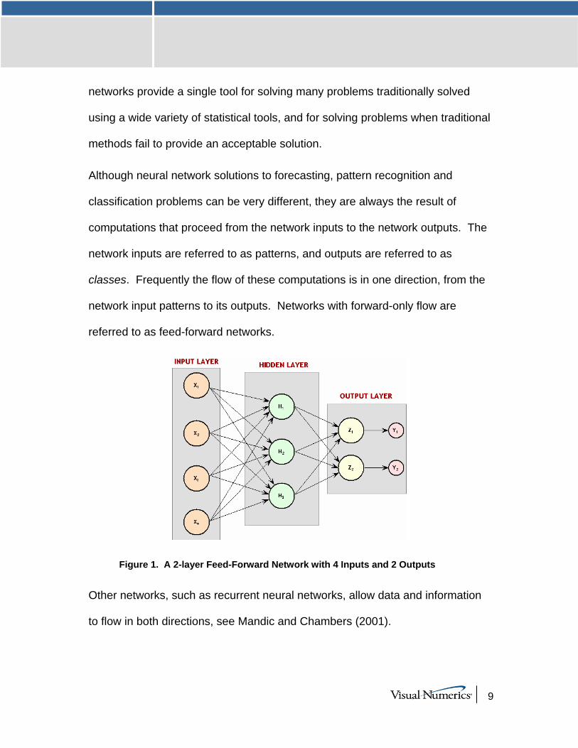
Although neural network solutions to forecasting, pattern recognition and

classification problems can be very different, they are always the result of

computations that proceed from the network inputs to the network outputs. The

network inputs are referred to as patterns, and outputs are referred to as

classes. Frequently the flow of these computations is in one direction, from the

network input patterns to its outputs. Networks with forward-only flow are

referred to as feed-forward networks.

Figure 1. A 2-layer Feed-Forward Network with 4 Inputs and 2 Outputs

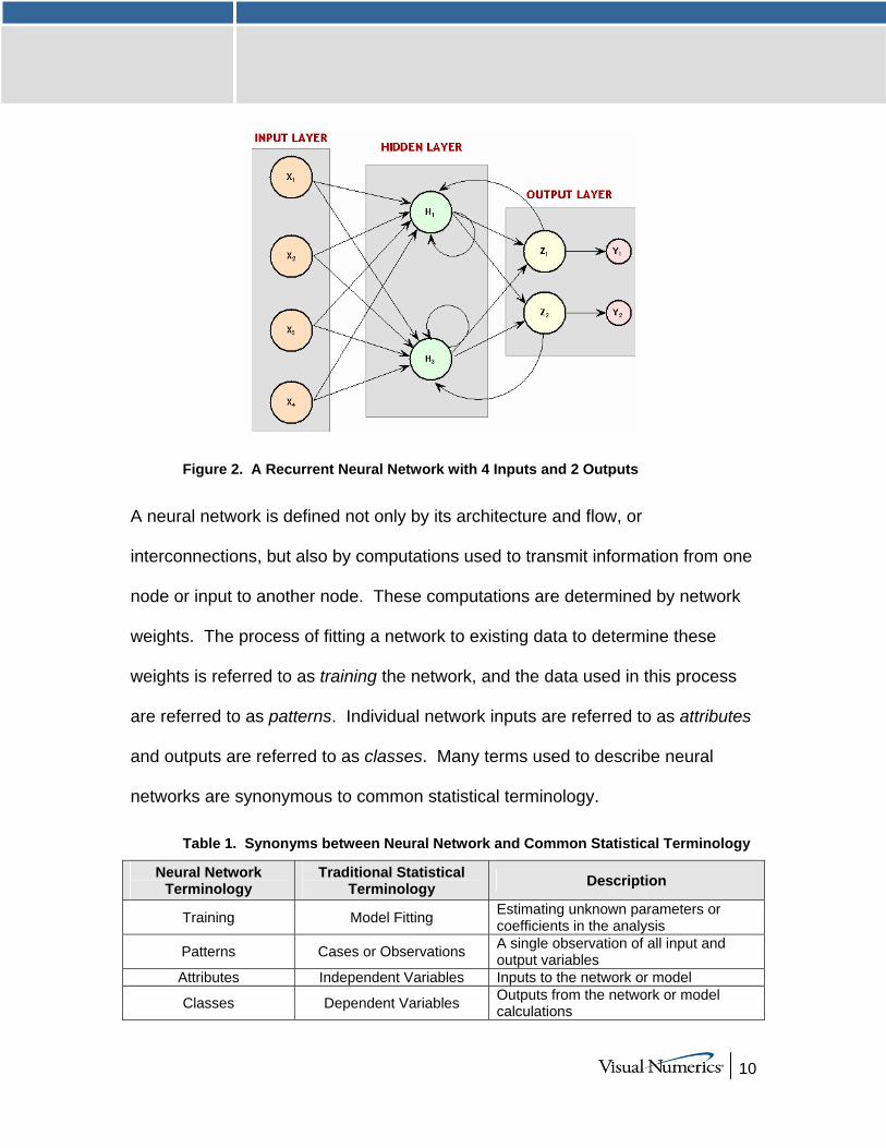
Other networks, such as recurrent neural networks, allow data and information

to flow in both directions, see Mandic and Chambers (2001).

10

Figure 2. A Recurrent Neural Network with 4 Inputs and 2 Outputs

A neural network is defined not only by its architecture and flow, or

interconnections, but also by computations used to transmit information from one

node or input to another node. These computations are determined by network

weights. The process of fitting a network to existing data to determine these

weights is referred to as training the network, and the data used in this process

are referred to as patterns. Individual network inputs are referred to as attributes

and outputs are referred to as classes. Many terms used to describe neural

networks are synonymous to common statistical terminology.

Table 1. Synonyms between Neural Network and Common Statistical Terminology

Neural Network Terminology

Traditional Statistical Terminology Description

Training Model Fitting Estimating unknown parameters or coefficients in the analysis

Patterns Cases or Observations A single observation of all input and output variables

Attributes Independent Variables Inputs to the network or model

Classes Dependent Variables Outputs from the network or model calculations

11

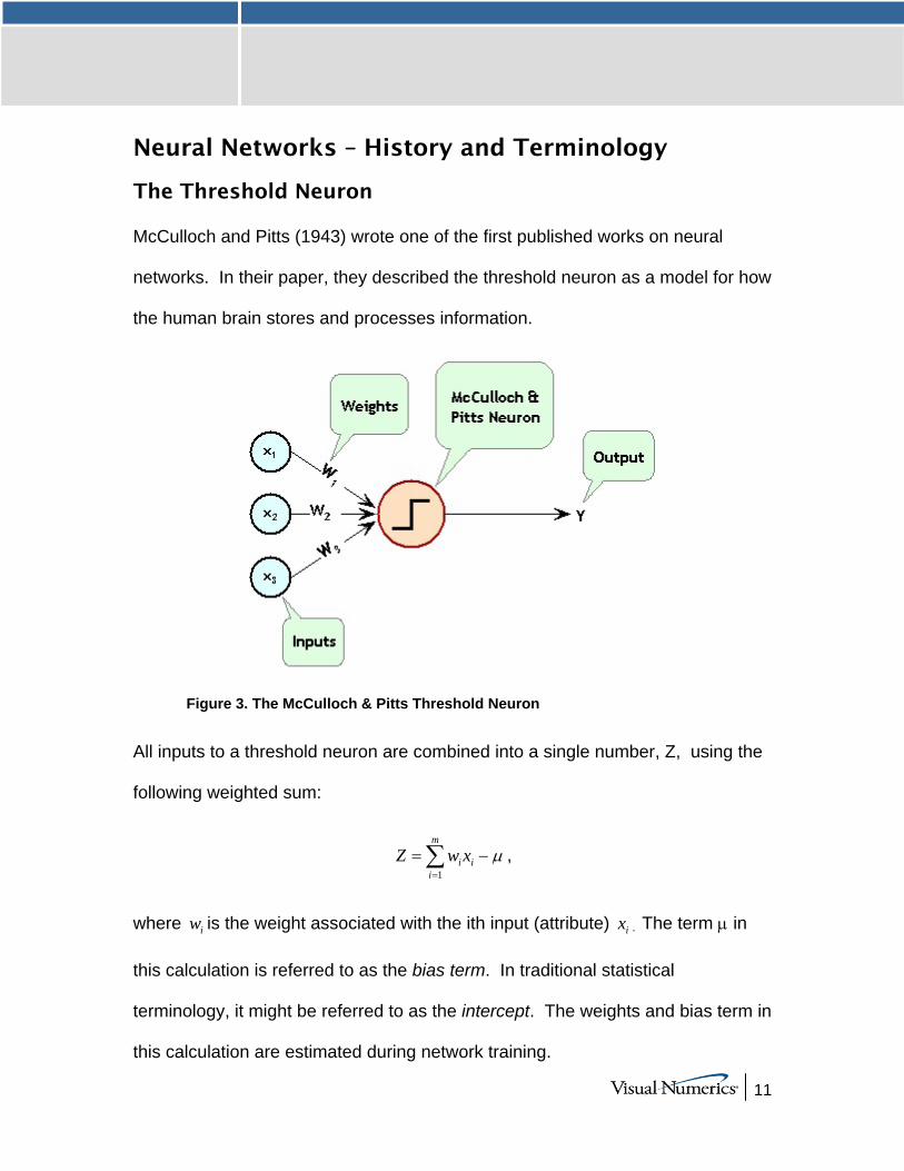
Neural Networks – History and Terminology

The Threshold Neuron McCulloch and Pitts (1943) wrote one of the first published works on neural

networks. In their paper, they described the threshold neuron as a model for how

the human brain stores and processes information.

Figure 3. The McCulloch & Pitts Threshold Neuron

All inputs to a threshold neuron are combined into a single number, Z, using the

following weighted sum:

1

m

i ii

Z w x µ=

= −∑ ,

where iw is the weight associated with the ith input (attribute) ix . The term µ in

this calculation is referred to as the bias term. In traditional statistical

terminology, it might be referred to as the intercept. The weights and bias term in

this calculation are estimated during network training.

12

In McCulloch and Pitt’s description of the threshold neuron, the neuron does not

respond to its inputs unless Z is greater than zero. If Z is greater than zero then

the output from this neuron is set equal to 1. If Z is less than zero the output is

zero:

1 if 00 if 0

ZY

Z>⎧

= ⎨ ≤⎩,

where Y is the neuron’s output.

For years following their 1943 paper, interest in the McCulloch and Pitts neural

network was limited to theoretical discussions, such as those of Hebb (1949),

about learning, memory and the brain’s structure.

The Perceptron The McCulloch and Pitts neuron is also referred to as a threshold neuron since it

abruptly changes its output from 0 to 1 when its potential, Z, crosses a threshold.

Mathematically, this behavior can be viewed as a step function that maps the

neuron’s potential, Z, to the neuron’s output, Y.

Rosenblatt (1958) extended the McCulloch and Pitts threshold neuron by

replacing this step function with a continuous function that maps Z to Y. The

Rosenblatt neuron is referred to as the perceptron, and the continuous function

mapping Z to Y makes it easier to train a network of perceptrons than a network

of threshold neurons.

Unlike the threshold neuron, the perceptron produces analog output rather than

the threshold neuron’s purely binary output. With careful selection of the analog

13

function, this makes Rosenblatt’s perceptron differentiable, whereas the

threshold neuron is not. This simplifies the training algorithm.

Like the threshold neuron, Rosenblatt’s perceptron starts by calculating a

weighted sum of its inputs, 1

m

i ii

Z w x µ=

= −∑ . This is referred to as the perceptron’s

potential.

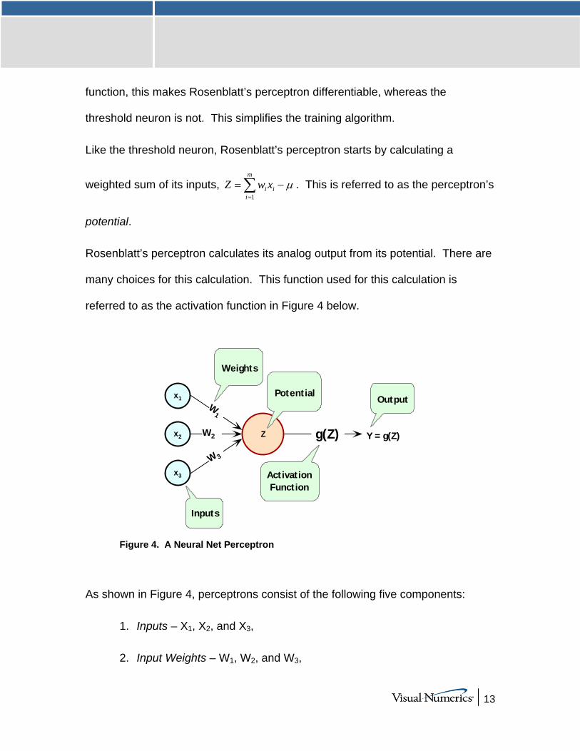
Rosenblatt’s perceptron calculates its analog output from its potential. There are

many choices for this calculation. This function used for this calculation is

referred to as the activation function in Figure 4 below.

g(Z)

x1

Zx2

x3

W1

W2

W 3

ActivationFunction

Potential

Weights

Inputs

Y = g(Z)

Output

Figure 4. A Neural Net Perceptron

As shown in Figure 4, perceptrons consist of the following five components:

1. Inputs – X1, X2, and X3,

2. Input Weights – W1, W2, and W3,

14

3. Potential - 3

1i i

i

Z W X µ=

= −∑ , where µ is a bias correction,

4. Activation Function – g(Z), and

5. Output – Y = g(Z) .

Like threshold neurons, perceptron inputs can either be the initial raw data inputs

or the output from another perceptron. The primary purpose of network training

is to estimate the weights associated with each perceptron’s potential. The

activation function maps this potential to the perceptron’s output.

The Activation Function Although theoretically any differential function can be used as an activation

function, the identity and sigmoid functions are the two most commonly used.

The identity activation function, also referred to as linear activation, is a flow-

through mapping of the perceptron’s potential to its output:

( )g Z Z= .

Output perceptrons in a forecasting network often use the identity activation

function.

Figure 5. An Identity (Linear) Activation Function

15

If the identity activation function is used throughout the network, then it is easily

shown that the network is equivalent to some fitting a linear regression model of

the form 0 1 1i k kY x xβ β β= + + +L , where 1 2, , , kx x xL are the k network inputs, iY is

the ith network output and 0 1, , , kβ β βL are the coefficients in the regression

equation. As a result, it is uncommon to find a neural network with identity

activation used in all its perceptrons.

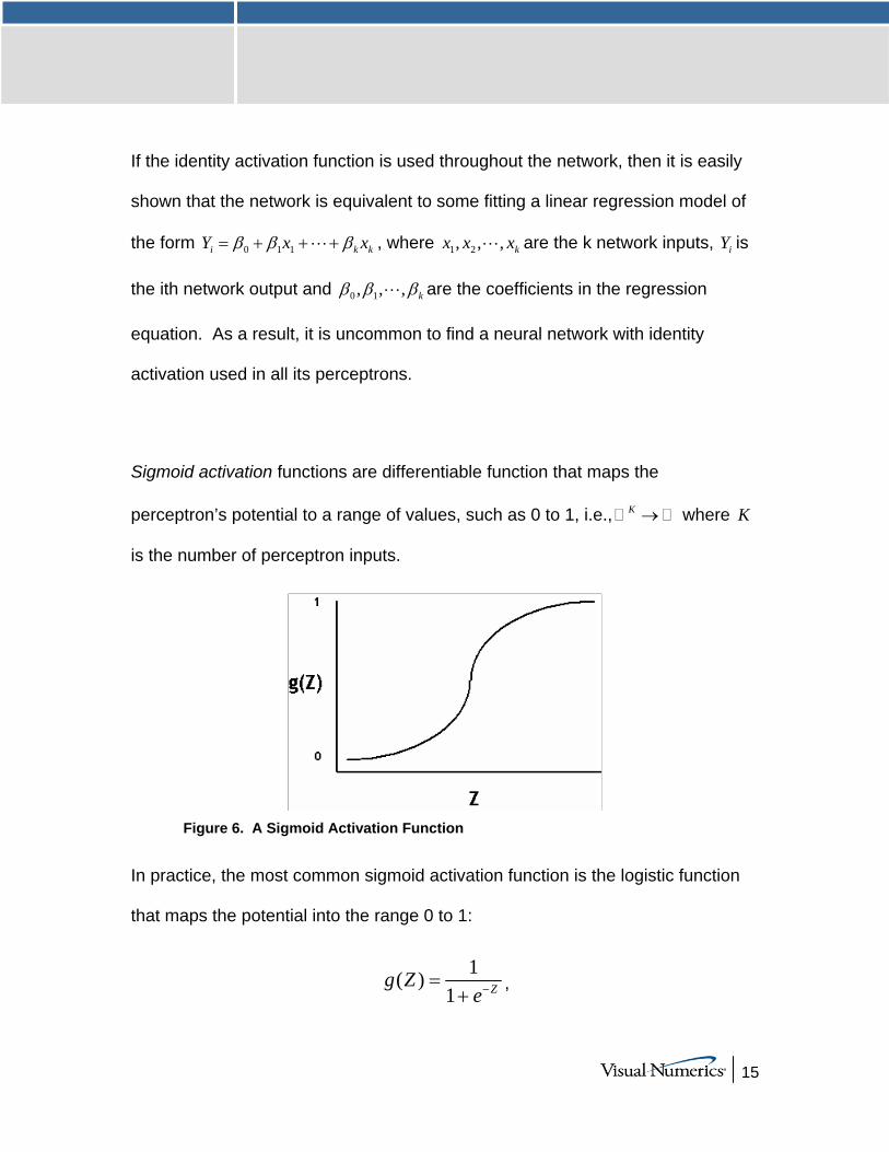
Sigmoid activation functions are differentiable function that maps the

perceptron’s potential to a range of values, such as 0 to 1, i.e., K → where K

is the number of perceptron inputs.

Figure 6. A Sigmoid Activation Function

In practice, the most common sigmoid activation function is the logistic function

that maps the potential into the range 0 to 1:

1( )1 Zg Z

e−=+

,

16

Since 0 < g(Z) < 1, the logistic function is very popular for use in networks that

output probabilities.

Other popular sigmoid activation functions include:

1. The hyperbolic-tangent ( ) tanh( )Z Z

Z Z

e eg Z Ze e

α α

α α

−

−

−= =

+,

2. The arc-tangent 2( ) arctan2Zg Z π

π⎛ ⎞= ⎜ ⎟⎝ ⎠

,

3. The squash activation function (Elliott (1993)) ( )1

Zg ZZ

=+

.

It is easy to show that the hyperbolic-tangent and logistic activation functions are

linearly related. Consequently forecasts produced using logistic activation should

be close to those produced using hyperbolic-tangent activation. However, one

function may be preferred over the other when training performance is a concern.

Researchers report that the training time using the hyperbolic-tangent activation

function is shorter than using the logistic activation function.

Network Applications

Forecasting using Neural Networks There are many good statistical forecasting tools. Most require assumptions

about the relationship between the variables being forecasted and the variables

used to produce the forecast, as well as the distribution of forecast errors. Such

statistical tools are referred to as parametric methods. ARIMA time series

models, for example, assume that the time series is stationary, that the errors in

17

the forecasts follow a particular ARIMA model, and that the probability

distribution for the residual errors is Gaussian, see Box and Jenkins (1970). If

these assumptions are invalid, then ARIMA time series forecasts can be very

poor.

Neural networks, on the other hand, require few assumptions. Since neural

networks can approximate highly non-linear functions, they can be applied

without an extensive analysis of underlying assumptions.

Another advantage of neural networks over ARIMA modeling is the number of

observations needed to produce a reliable forecast. ARIMA models generally

require 50 or more equally spaced, sequential observations in time. In many

cases, neural networks can also provide adequate forecasts with fewer

observations by incorporating exogenous, or external, variables in the network’s

input.

For example, a company applying ARIMA time series analysis to forecast

business expenses would normally require each of its departments, and each

sub-group within each department to prepare its own forecast. For large

corporations this can require fitting hundreds or even thousands of ARIMA

models. With a neural network approach, the department and sub-group

information could be incorporated into the network as exogenous variables.

Although this can significantly increase the network’s training time, the result

would be a single model for predicting expenses within all departments and sub-

departments.

18

Linear least squares models are also popular statistical forecasting tools. These

methods range from simple linear regression for predicting a single quantitative

outcome to logistic regression for estimating probabilities associated with

categorical outcomes. It is easy to show that simple linear least squares

forecasts and logistic regression forecasts are equivalent to a feed-forward

network with a single layer. For this reason, single-layer feed-forward networks

are rarely used for forecasting. Instead multilayer networks are used.

Hutchinson (1994) and Masters (1995) describe using multilayer feed-forward

neural networks for forecasting. Multilayer feed-forward networks are

characterized by the forward-only flow of information in the network. The flow of

information and computations in a feed-forward network is always in one

direction, mapping an M-dimensional vector of input to a C-dimensional vector of

outputs, i.e., M C→ where C M< .

There are many other types of networks without this feed-forward requirement.

Information and computations in a recurrent neural network, for example, flows in

both directions. Output from one level of a recurrent neural network can be fed

back, with some delay, as input into the same network, see Figure 2. Recurrent

networks are very useful for time series prediction, see Mandic and Chambers

(2001).

Pattern Recognition using Neural Networks Neural networks are also extensively used in statistical pattern recognition.

Pattern recognition applications that make wide use of neural networks include:

19

• natural language processing: Manning and Schütze (1999)

• speech and text recognition: Lippmann (1989)

• face recognition: Lawrence, et al. (1997)

• playing backgammon, Tesauro (1990)

• classifying financial news, Calvo (2001).

The interest in pattern recognition using neural networks has stimulated the

development of important variations of feed-forward networks. Two of the most

popular are:

• Self-Organizing Maps, also called Kohonen Networks, Kohonen (1995),

• and Radial Basis Function Networks, Bishop (1995).

Good mathematical descriptions of the neural network methods underlying these

applications are given by Bishop (1995), Ripley (1996), Mandic and Chambers

(2001), and Abe (2001). An excellent overview of neural networks, from a

statistical viewpoint, is also found in Warner and Misra (1996).

Neural Networks for Classification Classifying observations using prior concomitant information is possibly the most

popular application of neural networks. Data classification problems abound in

many businesses and research. When decisions based upon data are needed,

they can often be treated as a neural network data classification problem.

Decisions to buy, sell, hold or do nothing with a stock, are decisions involving

20

four choices. Classifying loan applicants as good or bad credit risks, based upon

their application, is also a classification problem involving two choices. Neural

networks are powerful tools for making decisions or choices based upon data.

These same tools are great for automatic selection or decision-making.

Incoming email, for example, can be examined to separate spam from important

email using a neural network trained for this task. A good overview of solving

classification problems using multilayer feed-forward neural networks is found in

Abe (2001) and Bishop (1995).

There are two popular methods for solving data classification problems using

multilayer feed-forward neural networks, depending upon the number of choices

(classes) in the classification problem. If the classification problem involves only

two choices, then the classification problem can be solved using a neural

network with one logistic output. This output estimates the probability that the

input data belong to one of the two choices.

For example, a multilayer feed-forward network with a single logistic output can

be used to determine whether a new customer is credit-worthy. The network’s

input would consist of information on the applicants credit application, such as

age, income, etc. If the network output probability is above some threshold value

(such as 0.5 or higher) then the applicant’s credit application is approved.

This is referred to as binary classification using a multilayer feed-forward neural

network. If more than two classes are involved then a different approach is

needed. A popular approach is to assign logistic output perceptrons to each

21

class in the classification problem. The network assigns each input pattern to the

class associated with the output perceptron that has the highest probability for

that input pattern. However, this approach produces invalid probabilities since

the sum of the individual class probabilities for each input is not equal to one,

which is a requirement for any valid multivariate probability distribution.

To avoid this problem, the softmax activation function, see Bridle (1990), applied

to the network outputs ensures that the outputs conform to the mathematical

requirements of multivariate classification probabilities. If the classification

problem has C categories, or classes, then each category is modeled by one of

the network outputs. If Zi is the weighted sum of products between its weights

and inputs for the ith output, i.e., i ji jij

Z w y= ∑ then

i

1

esoftmaxi

j

Z

CZ

j

e=

=

∑.

The softmax activation function ensures that the outputs all conform to the

requirements for multivariate probabilities. That is,

1. 0 < softmaxi< 1, for all i = 1, 2, …, C and

2. C

ii=1

softmax 1=∑

A pattern is assigned to the ith classification when softmaxi is the largest among

all C classes.

22

However, multilayer feed-forward neural networks are only one of several

popular methods for solving classification problems. Others include:

• Support Vector Machines (SVM Neural Networks), Abe (2001),

• Classification and Regression Trees (CART), Breiman, et al. (1984),

• Quinlan’s classification algorithms C4.5 and C5.0, Quinlan (1993), and

• Quick, Unbiased and Efficient Statistical Trees (QUEST), Loh and Shih

(1997).

Support Vector Machines are simple modifications of traditional multilayer feed-

forward neural networks (MLFF) configured for pattern classification.

Multilayer Feed-Forward Neural Networks A multilayer feed-forward neural network is an interconnection of perceptrons in

which data and calculations flow in a single direction, from the input data to the

outputs. The number of layers in a neural network is the number of layers of

perceptrons. The simplest neural network is one with a single input layer and an

output layer of perceptrons. The network in Figure 7 illustrates this type of

network. Technically this is referred to as a one-layer feed-forward network with

two outputs because the output layer is the only layer with an activation

calculation.

23

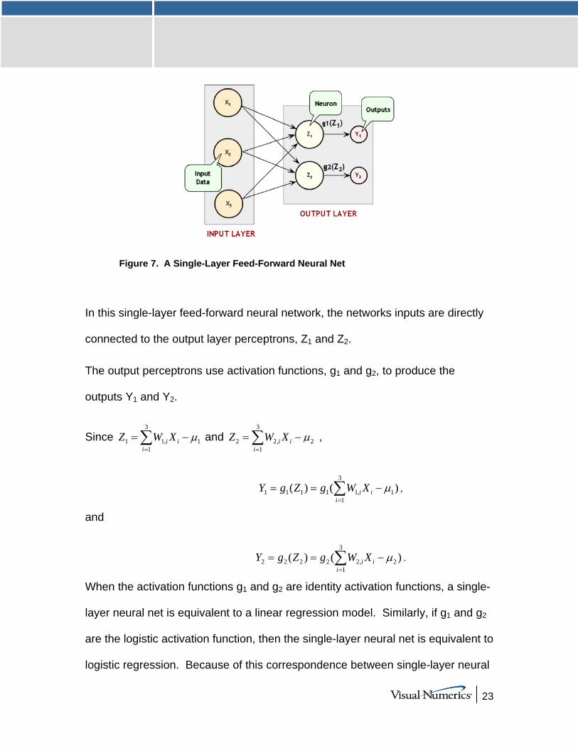
Figure 7. A Single-Layer Feed-Forward Neural Net

In this single-layer feed-forward neural network, the networks inputs are directly

connected to the output layer perceptrons, Z1 and Z2.

The output perceptrons use activation functions, g1 and g2, to produce the

outputs Y1 and Y2.

Since 3

1 1, 11

i ii

Z W X µ=

= −∑ and 3

2 2, 21

i ii

Z W X µ=

= −∑ ,

3

1 1 1 1 1, 11

( ) ( )i ii

Y g Z g W X µ=

= = −∑ ,

and

3

2 2 2 2 2, 21

( ) ( )i ii

Y g Z g W X µ=

= = −∑ .

When the activation functions g1 and g2 are identity activation functions, a single-

layer neural net is equivalent to a linear regression model. Similarly, if g1 and g2

are the logistic activation function, then the single-layer neural net is equivalent to

logistic regression. Because of this correspondence between single-layer neural

24

networks and linear and logistic regression, single-layer neural networks are

rarely used in place of linear and logistic regression.

The next most complicated neural network is one with two layers. This extra

layer is referred to as a hidden layer. In general there is no restriction on the

number of hidden layers. However, it has been shown mathematically that a

two-layer neural network, such as Figure 6 below, can accurately reproduce any

differentiable function, provided the number of perceptrons in the hidden layer is

unlimited.

However, increasing the number of neurons increases the number of weights

that must be estimated in the network, which in turn increases the execution time

for this network. Instead of increasing the number of perceptrons in the hidden

layers to improve accuracy, it is sometimes better to add additional hidden

layers, which typically reduces both the total number of network weights and the

computational time. However, in practice, it is uncommon to see neural networks

with more than two or three hidden layers.

Neural Network Error Calculations

Error Calculations for Forecasting The error calculations used to train a neural network are very important. Many

error calculations have been researched, trying to find a calculation with a short

training time that is appropriate for the network’s application. Typically error

calculations are very different depending primarily on the network’s application.

25

For forecasting, the most popular error function is the sum-of-squared errors, or

one of its scaled versions. This is analogous to using the minimum least squares

optimization criterion in linear regression. Like least squares, the sum-of-

squared errors is calculated by looking at the squared difference between what

the network predicts for each training pattern and the target value, or observed

value, for that pattern. Formally the equation is the same as one-half the

traditional least squares error:

( )212

1 1

ˆN C

ij iji j

E t t= =

= −∑∑ ,

where N is the total number of training cases, C is equal to the number of

network outputs, ijt is the observed output for the ith training case and the jth

network output, and ijt is the network’s forecast for that case.

Common practice recommends fitting a different network for each forecast

variable. That is, recommended practice is to use C=1 when using a multilayer

feed-forward neural network for forecasting. For classification problems with

more than two classes, it is common to associate one output with each

classification category, i.e., C=number of classes.

Notice that in ordinary least squares, the sum-of-squared errors is not multiplied

by one-half. Although this as no impact on the final solution, it significantly

reduces the number of computations required during training.

26

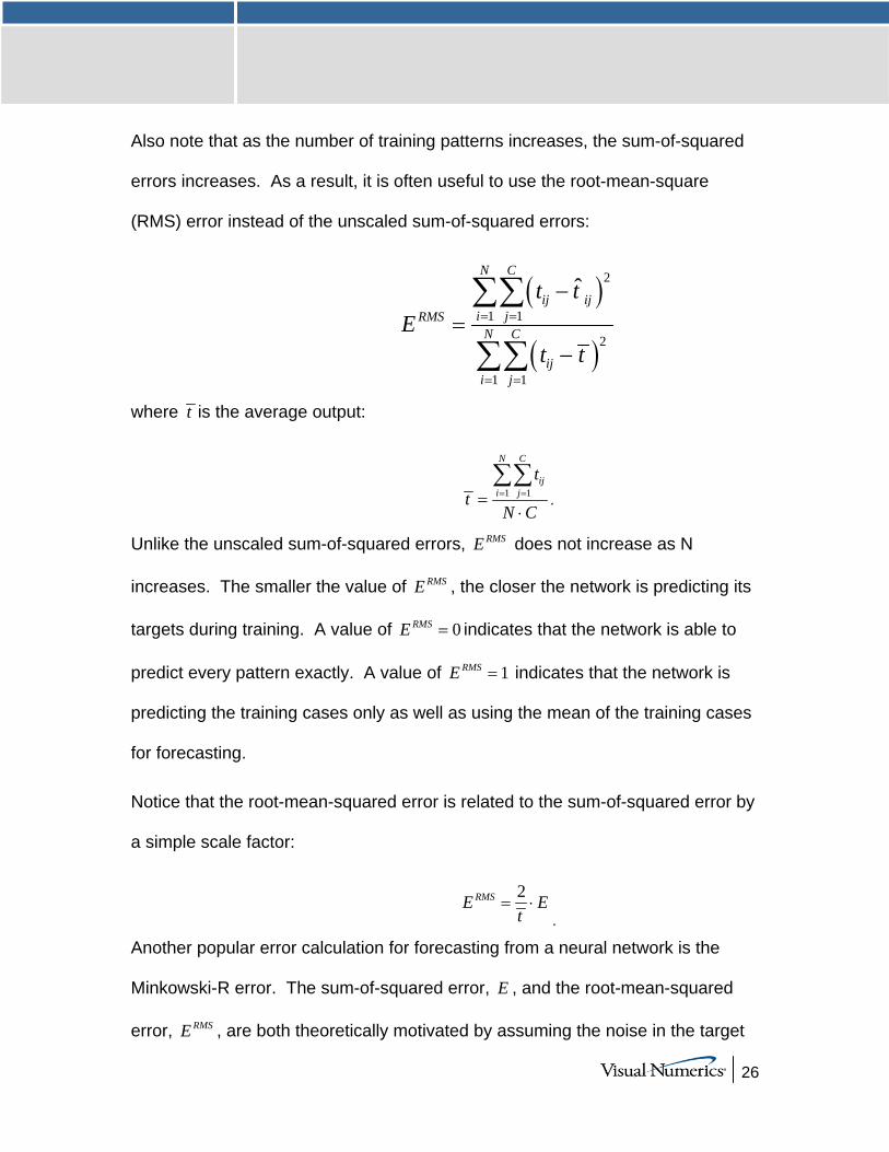
Also note that as the number of training patterns increases, the sum-of-squared

errors increases. As a result, it is often useful to use the root-mean-square

(RMS) error instead of the unscaled sum-of-squared errors:

( )

( )

2

1 1

2

1 1

ˆN C

ij iji jRMS

N C

iji j

t tE

t t

= =

= =

−=

−

∑∑

∑∑

where t is the average output:

1 1

N C

iji j

tt

N C= ==

⋅

∑∑.

Unlike the unscaled sum-of-squared errors, RMSE does not increase as N

increases. The smaller the value of RMSE , the closer the network is predicting its

targets during training. A value of 0RMSE = indicates that the network is able to

predict every pattern exactly. A value of 1RMSE = indicates that the network is

predicting the training cases only as well as using the mean of the training cases

for forecasting.

Notice that the root-mean-squared error is related to the sum-of-squared error by

a simple scale factor:

2RMSE Et

= ⋅.

Another popular error calculation for forecasting from a neural network is the

Minkowski-R error. The sum-of-squared error, E , and the root-mean-squared

error, RMSE , are both theoretically motivated by assuming the noise in the target

27

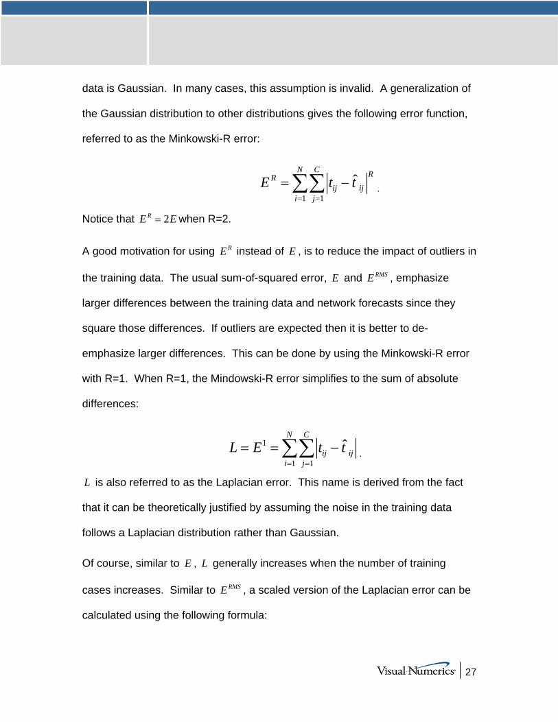
data is Gaussian. In many cases, this assumption is invalid. A generalization of

the Gaussian distribution to other distributions gives the following error function,

referred to as the Minkowski-R error:

1 1

ˆN C RR

ij iji j

E t t= =

= −∑∑ .

Notice that 2RE E= when R=2.

A good motivation for using RE instead of E , is to reduce the impact of outliers in

the training data. The usual sum-of-squared error, E and RMSE , emphasize

larger differences between the training data and network forecasts since they

square those differences. If outliers are expected then it is better to de-

emphasize larger differences. This can be done by using the Minkowski-R error

with R=1. When R=1, the Mindowski-R error simplifies to the sum of absolute

differences:

1

1 1

ˆN C

ij iji j

L E t t= =

= = −∑∑ .

L is also referred to as the Laplacian error. This name is derived from the fact

that it can be theoretically justified by assuming the noise in the training data

follows a Laplacian distribution rather than Gaussian.

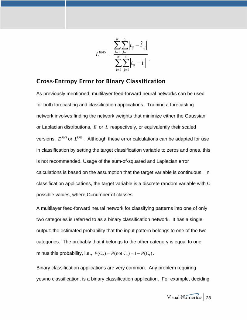
Of course, similar to E , L generally increases when the number of training

cases increases. Similar to RMSE , a scaled version of the Laplacian error can be

calculated using the following formula:

28

1 1

1 1

ˆN C

ij iji jRMS

N C

iji j

t tL

t t

= =

= =

−=

−

∑∑

∑∑ .

Cross-Entropy Error for Binary Classification As previously mentioned, multilayer feed-forward neural networks can be used

for both forecasting and classification applications. Training a forecasting

network involves finding the network weights that minimize either the Gaussian

or Laplacian distributions, E or L respectively, or equivalently their scaled

versions, RMSE or RMSL . Although these error calculations can be adapted for use

in classification by setting the target classification variable to zeros and ones, this

is not recommended. Usage of the sum-of-squared and Laplacian error

calculations is based on the assumption that the target variable is continuous. In

classification applications, the target variable is a discrete random variable with C

possible values, where C=number of classes.

A multilayer feed-forward neural network for classifying patterns into one of only

two categories is referred to as a binary classification network. It has a single

output: the estimated probability that the input pattern belongs to one of the two

categories. The probably that it belongs to the other category is equal to one

minus this probability, i.e., 2 1 1( ) (not C ) 1 ( )P C P P C= = − .

Binary classification applications are very common. Any problem requiring

yes/no classification, is a binary classification application. For example, deciding

29

to sell or buy a stock is a binary classification problem. Deciding to approve a

loan application is also a binary classification problem. Deciding whether to

approve a new drug or to provide one of two medical treatments are binary

classification problems.

For binary classification problems, only a single output is used, C=1. This output

represents the probability that the training case should be classified as “yes”. A

common choice for the activation function of the output of a binary classification

network is the logistic activation function, which always results in an output in the

range 0 to 1, regardless of the perceptron’s potential.

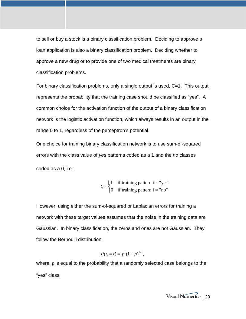
One choice for training binary classification network is to use sum-of-squared

errors with the class value of yes patterns coded as a 1 and the no classes

coded as a 0, i.e.:

1 if training pattern i = "yes"0 if training pattern i = "no"it⎧

= ⎨⎩

However, using either the sum-of-squared or Laplacian errors for training a

network with these target values assumes that the noise in the training data are

Gaussian. In binary classification, the zeros and ones are not Gaussian. They

follow the Bernoulli distribution:

1( ) (1 )t tiP t t p p −= = − ,

where p is equal to the probability that a randomly selected case belongs to the

“yes” class.

30

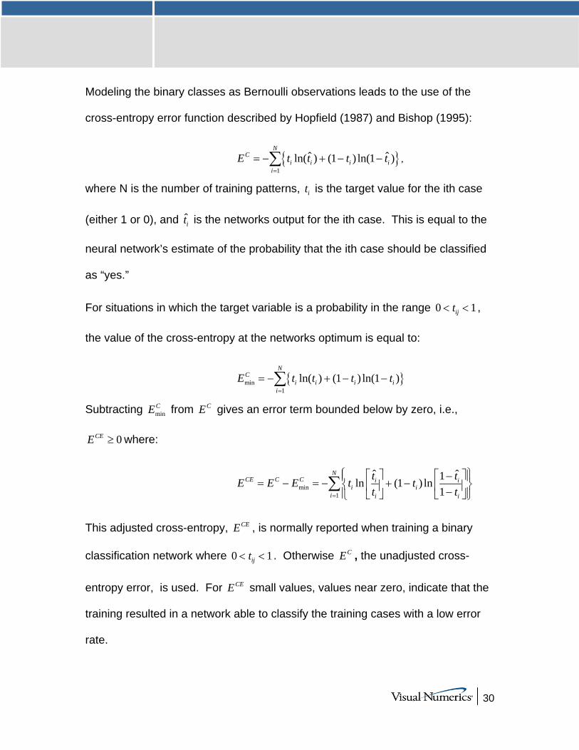
Modeling the binary classes as Bernoulli observations leads to the use of the

cross-entropy error function described by Hopfield (1987) and Bishop (1995):

{ }1

ˆ ˆln( ) (1 ) ln(1 )N

Ci i i i

i

E t t t t=

= − + − −∑ ,

where N is the number of training patterns, it is the target value for the ith case

(either 1 or 0), and it is the networks output for the ith case. This is equal to the

neural network’s estimate of the probability that the ith case should be classified

as “yes.”

For situations in which the target variable is a probability in the range 0 1ijt< < ,

the value of the cross-entropy at the networks optimum is equal to:

{ }min1

ln( ) (1 ) ln(1 )N

Ci i i i

i

E t t t t=

= − + − −∑

Subtracting minCE from CE gives an error term bounded below by zero, i.e.,

0CEE ≥ where:

min1

ˆ ˆ1ln (1 ) ln1

NCE C C i i

i ii i i

t tE E E t tt t=

⎧ ⎫⎡ ⎤ ⎡ ⎤−⎪ ⎪= − = − + −⎨ ⎬⎢ ⎥ ⎢ ⎥−⎪ ⎪⎣ ⎦ ⎣ ⎦⎩ ⎭∑

This adjusted cross-entropy, CEE , is normally reported when training a binary

classification network where 0 1ijt< < . Otherwise CE , the unadjusted cross-

entropy error, is used. For CEE small values, values near zero, indicate that the

training resulted in a network able to classify the training cases with a low error

rate.

31

Cross-Entropy Error for Multiple Classes Using a multilayer feed-forward neural network for binary classification is

relatively straightforward. A network for binary classification only has a single

output that estimates the probability that an input pattern belongs to the “yes”

class, i.e., 1it = . In classification problems with more than two mutually exclusive

classes, the calculations and network configurations are not as simple.

One approach is to use multiple network outputs, one for each of the C classes.

Using this approach, the jth output for the ith training pattern, ijt , is the estimated

probability that the ith pattern belongs to the jth class, denoted by ijt . An easy

way to estimate these probabilities is to use logistic activation for each output.

This ensures that each output satisfies the univariate probability requirements,

i.e., ˆ0 1ijt≤ ≤ .

However, since the classification categories are mutually exclusive, each pattern

can only be assigned to one of the C classes, which means that the sum of these

individual probabilities should always equal 1. However, if each output is the

estimated probability for that class, it is very unlikely that 1

ˆ 1C

ijj

t=

=∑ . In fact, the

sum of the individual probability estimates can easily exceed 1 if logistic

activation is applied to every output.

Support Vector Machine (SVM) neural networks use this approach with one

modification. A SVM network classifies a pattern as belonging to the ith category

32

if the activation calculation for that category exceeds a threshold and the other

calculations do not exceed this value. That is, the ith pattern is assigned to the

jth category if and only if ijt δ> and ikt δ≤ for all k j≠ , where δ is the threshold.

If this does not occur, then the pattern is marked as unclassified.

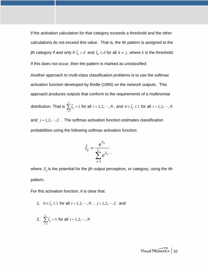
Another approach to multi-class classification problems is to use the softmax

activation function developed by Bridle (1990) on the network outputs. This

approach produces outputs that conform to the requirements of a multinomial

distribution. That is 1

ˆ 1C

ijj

t=

=∑ for all 1,2, ,i N= L , and ˆ0 1ijt≤ ≤ for all 1,2, ,i N= L

and 1,2, ,j C= L . The softmax activation function estimates classification

probabilities using the following softmax activation function:

1

eˆij

ij

Z

ij CZ

j

te

=

=

∑ ,

where ijZ is the potential for the jth output perceptron, or category, using the ith

pattern.

For this activation function, it is clear that:

1. ˆ0 1ijt≤ ≤ for all 1,2, ,i N= L , 1,2, ,j C= L and

2. 1

ˆ 1C

ijj

t=

=∑ for all 1,2, ,i N= L

33

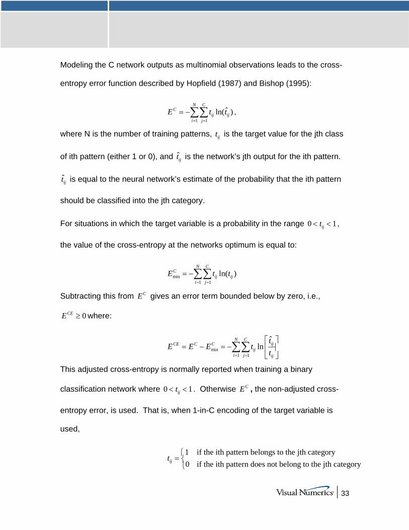
Modeling the C network outputs as multinomial observations leads to the cross-

entropy error function described by Hopfield (1987) and Bishop (1995):

1 1

ˆln( )N C

Cij ij

i j

E t t= =

= −∑∑ ,

where N is the number of training patterns, ijt is the target value for the jth class

of ith pattern (either 1 or 0), and ijt is the network’s jth output for the ith pattern.

ijt is equal to the neural network’s estimate of the probability that the ith pattern

should be classified into the jth category.

For situations in which the target variable is a probability in the range 0 1ijt< < ,

the value of the cross-entropy at the networks optimum is equal to:

min1 1

ln( )N C

Cij ij

i j

E t t= =

= −∑∑

Subtracting this from CE gives an error term bounded below by zero, i.e.,

0CEE ≥ where:

min1 1

ˆln

N CijCE C C

iji j ij

tE E E t

t= =

⎡ ⎤= − = − ⎢ ⎥

⎣ ⎦∑∑

This adjusted cross-entropy is normally reported when training a binary

classification network where 0 1ijt< < . Otherwise CE , the non-adjusted cross-

entropy error, is used. That is, when 1-in-C encoding of the target variable is

used,

1 if the ith pattern belongs to the jth category0 if the ith pattern does not belong to the jth categoryijt ⎧

= ⎨⎩

34

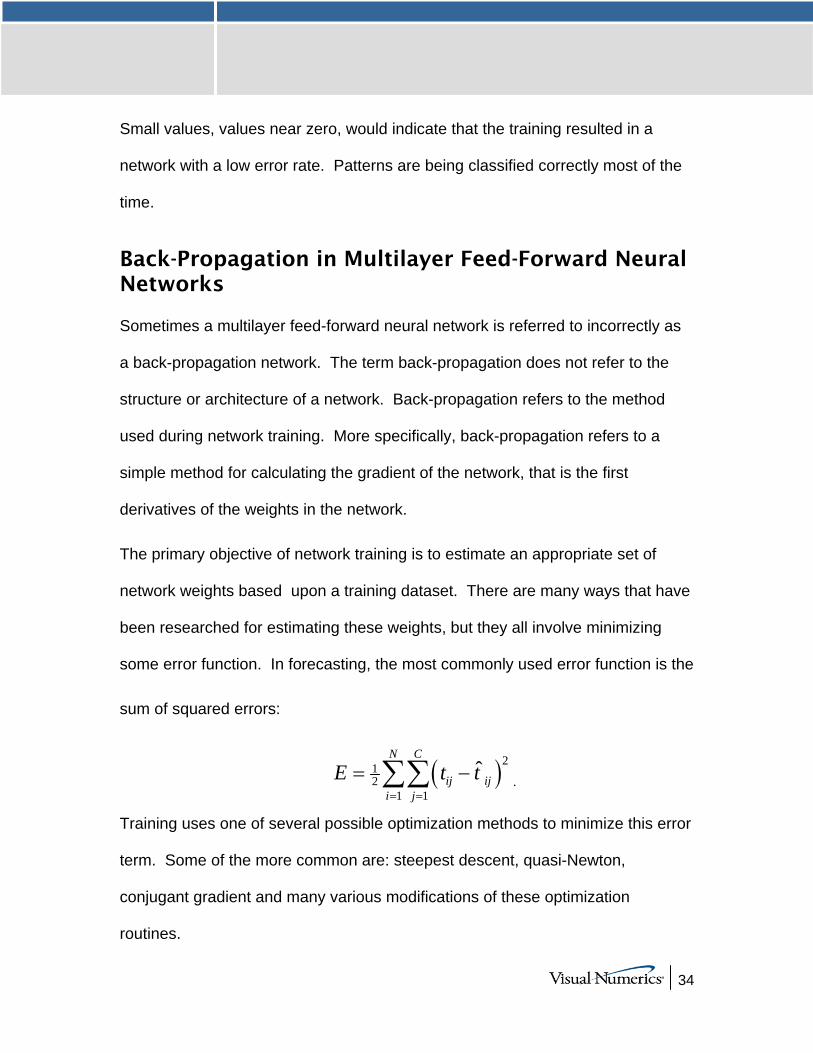
Small values, values near zero, would indicate that the training resulted in a

network with a low error rate. Patterns are being classified correctly most of the

time.

Back-Propagation in Multilayer Feed-Forward Neural Networks Sometimes a multilayer feed-forward neural network is referred to incorrectly as

a back-propagation network. The term back-propagation does not refer to the

structure or architecture of a network. Back-propagation refers to the method

used during network training. More specifically, back-propagation refers to a

simple method for calculating the gradient of the network, that is the first

derivatives of the weights in the network.

The primary objective of network training is to estimate an appropriate set of

network weights based upon a training dataset. There are many ways that have

been researched for estimating these weights, but they all involve minimizing

some error function. In forecasting, the most commonly used error function is the

sum of squared errors:

( )212

1 1

ˆN C

ij iji j

E t t= =

= −∑∑ .

Training uses one of several possible optimization methods to minimize this error

term. Some of the more common are: steepest descent, quasi-Newton,

conjugant gradient and many various modifications of these optimization

routines.

35

Back-propagation is a method for calculating the first derivatives, or gradient, of

the error function required by some optimization methods. It is certainly not the

only method for estimating the gradient. However, it is the most efficient. In fact,

some will argue that the development of this method by Werbos (1974), Parket

(1985) and Rumelhart, Hinton and Williams (1986) contributed to the popularity

of neural network methods by significantly reducing the network training time and

making it possible to train networks consisting of a large number of inputs and

perceptrons.

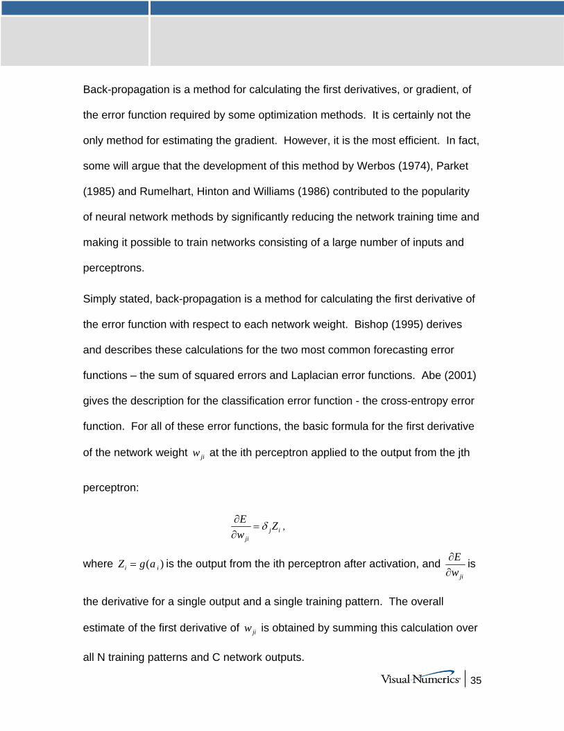
Simply stated, back-propagation is a method for calculating the first derivative of

the error function with respect to each network weight. Bishop (1995) derives

and describes these calculations for the two most common forecasting error

functions – the sum of squared errors and Laplacian error functions. Abe (2001)

gives the description for the classification error function - the cross-entropy error

function. For all of these error functions, the basic formula for the first derivative

of the network weight jiw at the ith perceptron applied to the output from the jth

perceptron:

j iji

E Zw

δ∂=

∂,

where ( )i iZ g a= is the output from the ith perceptron after activation, and ji

Ew∂∂

is

the derivative for a single output and a single training pattern. The overall

estimate of the first derivative of jiw is obtained by summing this calculation over

all N training patterns and C network outputs.

36

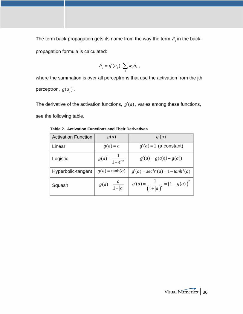
The term back-propagation gets its name from the way the term jδ in the back-

propagation formula is calculated:

( )j j kj kk

g a wδ δ′= ⋅∑ ,

where the summation is over all perceptrons that use the activation from the jth

perceptron, ( )jg a .

The derivative of the activation functions, ( )g a′ , varies among these functions,

see the following table.

Table 2. Activation Functions and Their Derivatives

Activation Function ( )g a ( )g a′

Linear ( )g a a= ( ) 1g a′ = (a constant)

Logistic 1( )

1 ag ae−=

+ ( ) ( )(1 ( ))g a g a g a′ = −

Hyperbolic-tangent ( ) tanh( )g a a= 2 2( ) ( ) 1 ( )g a sech a tanh a′ = = −

Squash ( )1

ag aa

=+

( )

( )2

21( ) 1 ( )

1g a g a

a′ = = −

+

37

References Abe, S. (2001) Pattern Classification: Neuro-Fuzzy Methods and their Comparison, Springer-Verlag. Berry, M. J. A. and Linoff, G. (1997) Data Mining Techniques, John Wiley & Sons, Inc. Bridle, J. S. (1990) Probabilistic Interpretation of Feedforward Classification Network Outputs, with relationships to statistical pattern recognition, in F. Fogelman Soulie and J. Herault (Eds.), Neuralcomputing: Algorithms, Architectures and Applications, Springer-Verlag, 227-236. Bishop, C. M. (1995) Neural Networks for Pattern Recognition, Oxford University Press. Box, G. E. P. and Jenkins, G. M. (1970) Time Series Analysis: Forecasting and Control, Holden-Day, Inc. Breiman, L., Friedman, J. H., Olshen, R. A. and Stone, C. J. (1984) Classification and Regression Trees, Chapman & Hall. For the latest information on CART visit http://www.salford-systems.com/index.html. Calvo, R. A. (2001) Classifying Financial News with Neural Networks, Proceedings of the 6th Australasian Document Computing Symposium. Elman, J. L. (1990) Finding Structure in Time, Cognitive Science, 14, 179-211. Giudici, P. (2003) Applied Data Mining: Statistical Methods for Business and Industry, John Wiley & Sons, Inc. Hebb, D. O. (1949) The Organization of Behaviour: A Neuropsychological Theory, John Wiley. Hopfield, J. J. (1987) Learning Algorithms and Probability Distributions in Feed-Forward and Feed-Back Networks, Proceedings of the National Academy of Sciences, 84, 8429-8433. Hutchinson, J. M. (1994) A Radial Basis Function Approach to Financial Timer Series Analysis, Ph.D. dissertation, Massachusetts Institute of Technology. Hwang, J. T. G. and Ding, A. A. (1997) Prediction Intervals for Artificial Neural Networks, Journal of the American Statistical Society, 92(438) 748-757. Jacobs, R. A., Jorday, M. I., Nowlan, S. J., and Hinton, G. E. (1991) Adaptive Mixtures of Local Experts, Neural Computation, 3(1), 79-87. Kohonen, T. (1995) Self-Organizing Maps, Springer-Verlag. Lawrence, S., Giles, C. L, Tsoi, A. C., Back, A. D. (1997) Face Recognition: A Convolutional Neural Network Approach, IEEE Transactions on Neural

38

Networks, Special Issue on Neural Networks and Pattern Recognition, 8(1), 98-113. Li, L. K. (1992) Approximation Theory and Recurrent Networks, Proc. Int. Joint Conf. On Neural Networks, vol. II, 266-271. Lippmann, R. P. (1989) Review of Neural Networks for Speech Recognition, Neural Computation, I, 1-38. Loh, W.-Y. and Shih, Y.-S. (1997) Split Selection Methods for Classification Trees, Statistica Sinica, 7, 815-840. For information on the latest version of QUEST see http://www.stat.wisc.edu/~loh/quest.html. Mandic, D. P. and Chambers, J. A. (2001) Recurrent Neural Networks for Prediction, John Wiley & Sons, LTD. Manning, C. D. and Schütze, H. (1999) Foundations of Statistical Natural Language Processing, MIT Press. McCulloch, W. S. and Pitts, W. (1943) A Logical Calculus for Ideas Imminent in Nervous Activity, Bulletin of Mathematical Biophysics, 5, 115-133. Pao, Y. (1989) Adaptive Pattern Recognition and Neural Networks, Addison-Wesley Publishing. Poli, I. and Jones, R. D. (1994) A Neural Net Model for Prediction, Journal of the American Statistical Society, 89(425) 117-121. Quinlan, J. R. (1993). C4.5 Programs for Machine Learning, Morgan Kaufmann. For the latest information on Quinlan’s algorithms see http://www.rulequest.com/. Reed, R. D. and Marks, R. J. II (1999) Neural Smithing: Supervised Learning in Feedforward Artificial Neural Networks, The MIT Press, Cambridge, MA. Ripley, B. D. (1994) Neural Networks and Related Methods for Classification, Journal of the Royal Statistical Society B, 56(3), 409-456. Ripley, B. D. (1996) Pattern Recognition and Neural Networks, Cambridge University Press. Rosenblatt, F. (1958) The Perceptron: A Probabilistic Model for Information Storage and Organization in the Brain, Psychol. Rev., 65, 386-408. Rumelhart, D. E., Hinton, G. E. and Williams, R. J. (1986) Learning Representations by Back-Propagating Errors, Nature, 323, 533-536. Rumelhart, D. E. and McClelland, J. L. eds. (1986) Parallel Distributed Processing: Explorations in the Microstructure of Cognition, 1, 318-362, MIT Press. Smith, M. (1993) Neural Networks for Statistical Modeling, New York: Van Nostrand Reinhold. Studenmund, A. H. (1992) Using Economics: A Practical Guide, New York: Harper Collins.

39

Swingler, K. (1996) Applying Neural Networks: A Practical Guide, Academic Press. Tesauro, G. (1990) Neurogammon Wins Computer Olympiad, Neural Computation, 1, 321-323. Warner, B. and Misra, M. (1996) Understanding Neural Networks as Statistical Tools, The American Statistician, 50(4) 284-293. Werbos, P. (1974) Beyond Regression: New Tools for Prediction and Analysis in the Behavioral Science, PhD thesis, Harvard University, Cambridge, MA. Werbos, P. (1990) Backpropagation Through Time: What It Does and How to do It, Proc. IEEE, 78, 1550-1560. Williams, R. J. and Zipser, D. (1989) A Learning Algorithm for Continuously Running Fully Recurrent Neural Networks, Neural Computation, 1, 270-280. Witten, I. H. and Frank, E. (2000) Data Mining: Practical Machine Learning Tools and Techniques with Java Implementations, Morgan Kaufmann Publishers. Wu, S-I (1995) Mirroring Our Thought Processes, IEEE Potentials, 14, 36-41.