Embed Size (px)
Citation preview
An introduction to Numerical Optimization
Stelian Coros
Plan for Today
• A fast and furious tour through numerical
optimization
– Unconstrained Optimization
• Gradient Descent
• Newton’s Method
– Constrained Optimization
• Newton’s Method
• Quadratic Programming
– Stochastic Optimization
– Discrete Optimization
Optimization in Graphics
• Simulation and Material Parameter Estimation
Introduction to Optimization
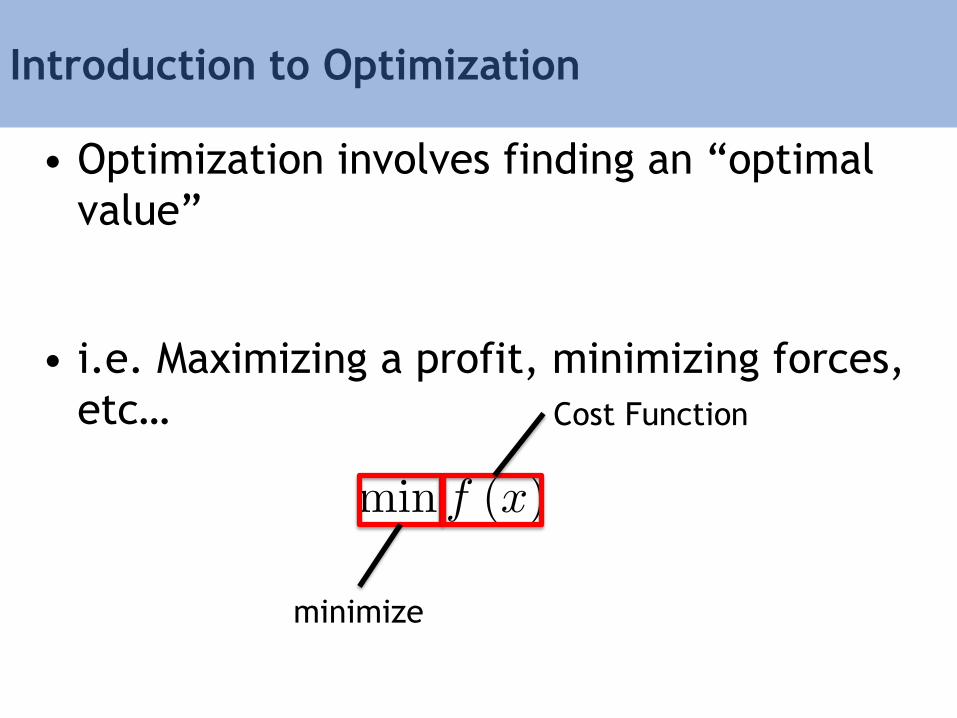
• Optimization involves finding an “optimal
value”
• i.e. Maximizing a profit, minimizing forces,
etc…
minimize
Cost Function

Introduction to Optimization
• Optimization involves finding an “optimal
value”
• i.e. Maximizing a profit, minimizing an
area etc…
Optimal Solution
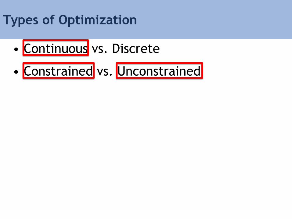
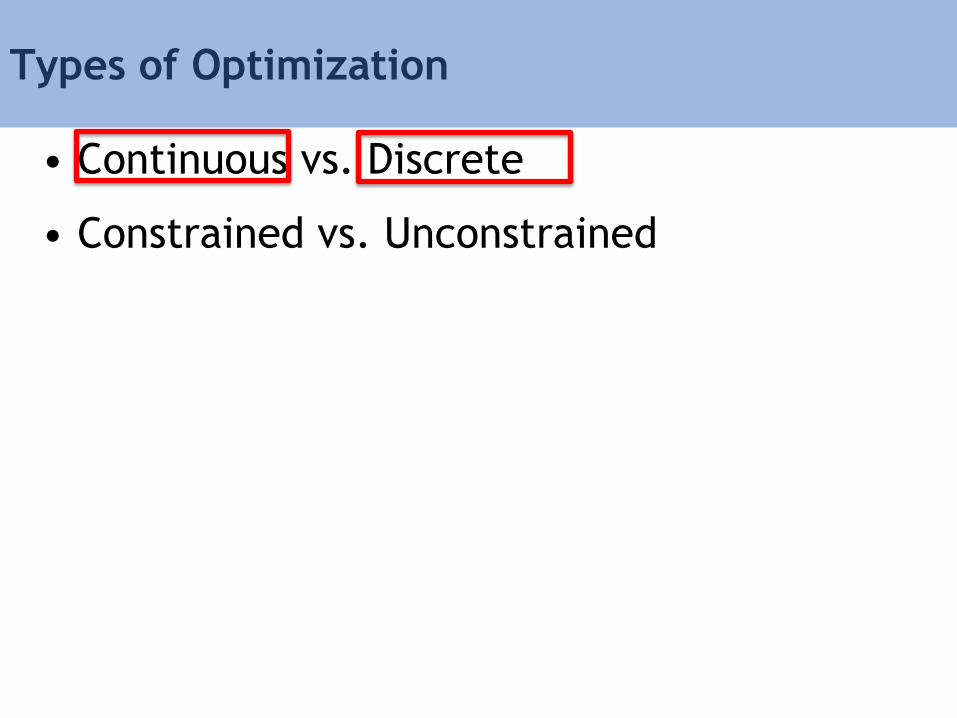
Types of Optimization
• Continuous vs. Discrete
• Constrained vs. Unconstrained

Continuous Discrete
This point can move
smoothly
Choose from discrete points in
parameter space
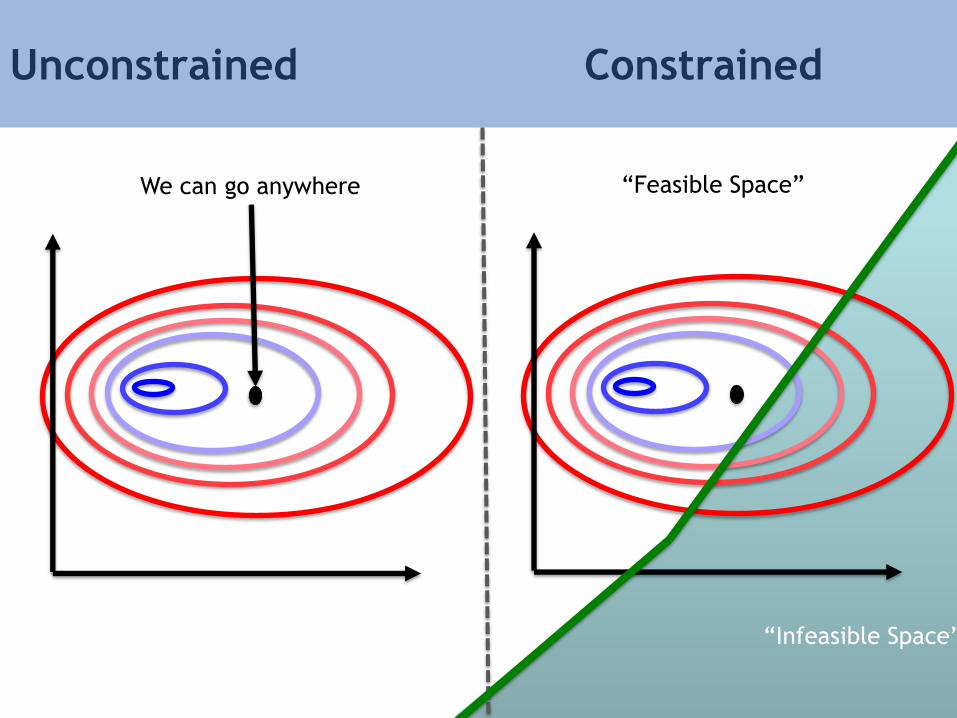
Unconstrained Constrained
We can go anywhere “Feasible Space”
“Infeasible Space”
Types of Optimization
• Continuous vs. Discrete
• Constrained vs. Unconstrained
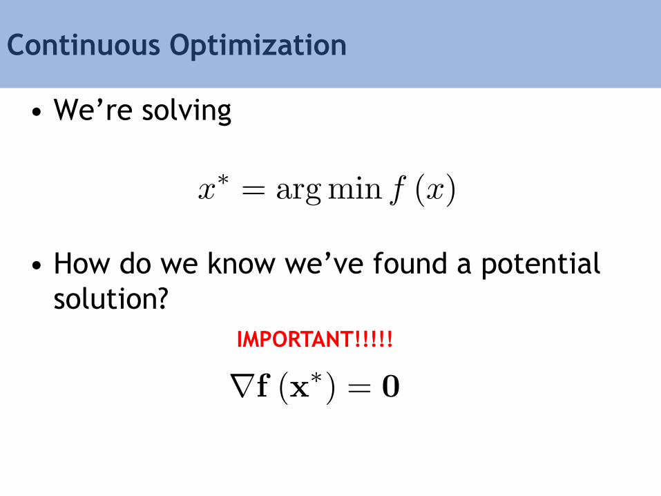
Continuous Optimization
• We’re solving
• How do we know we’ve found a potential
solution?
IMPORTANT!!!!!
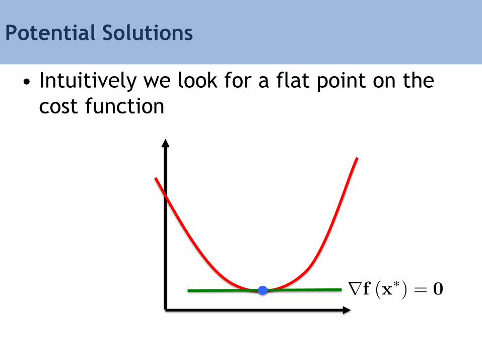
Potential Solutions
• Intuitively we look for a flat point on the
cost function
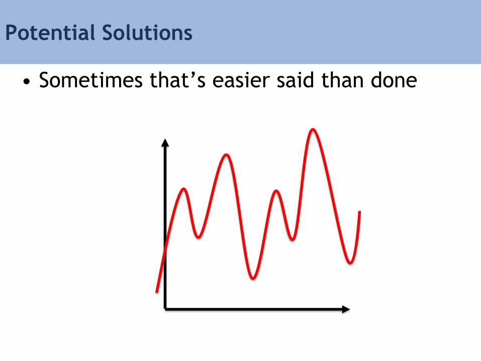
Potential Solutions
• Sometimes that’s easier said than done
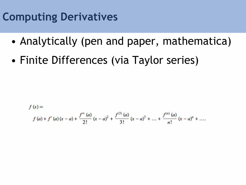
Computing Derivatives
• Analytically (pen and paper, mathematica)
• Finite Differences (via Taylor series)
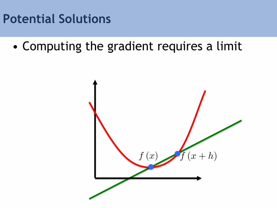
Potential Solutions
• Computing the gradient requires a limit
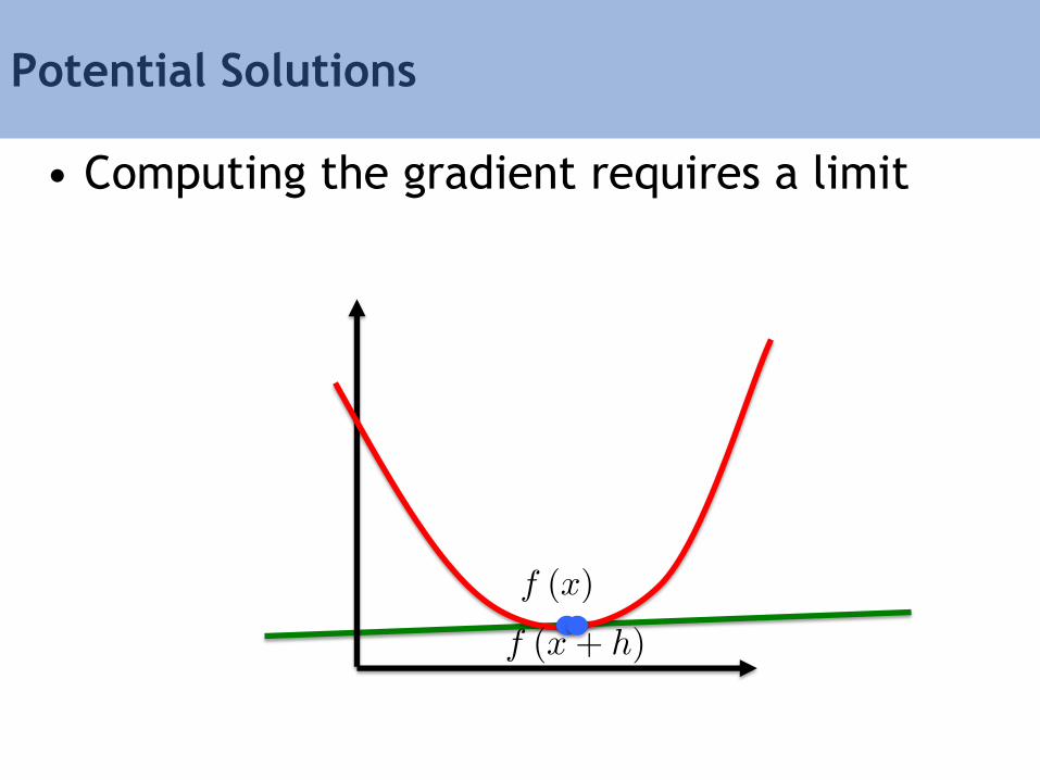
Potential Solutions
• Computing the gradient requires a limit
Potential Solutions
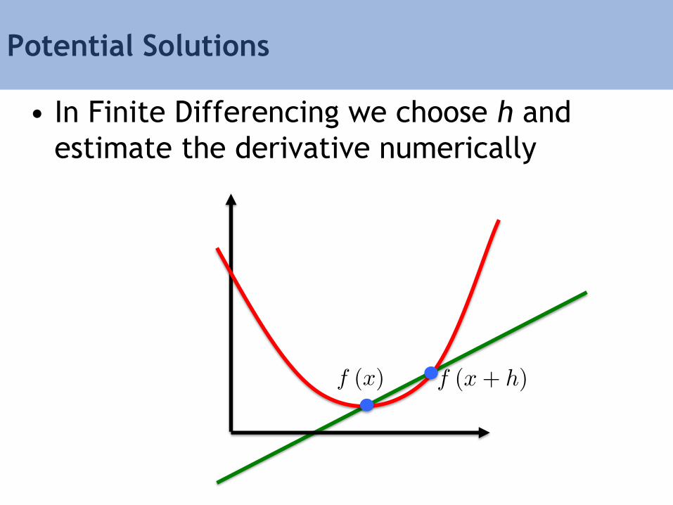
• In Finite Differencing we choose h and
estimate the derivative numerically
Continuous Optimization
• General, continuous optimizations are
difficult to solve – but we keep trying
anyway
• We focus on certain classes of problems
that are solvable
Convex Optimization
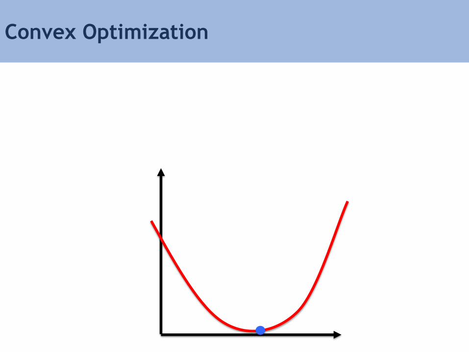
Convex Optimization
• Convex optimizations are ones that have a
single minimum
• Let’s look at some examples of convex
cost functions
Convex Optimization
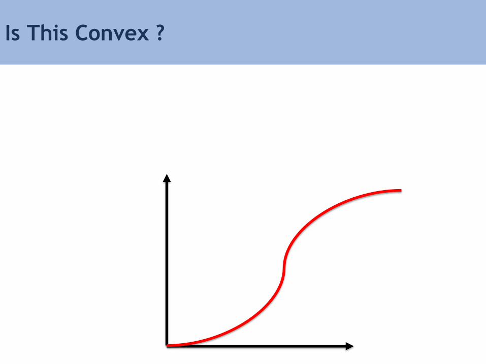
Is This Convex ?
Descent Algorithms
• Idea: Follow search directions that reduce
the cost!
• Two Types
– Gradient Descent
– Newton’s Method
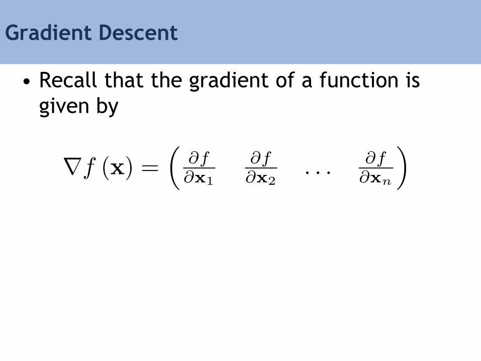
Gradient Descent
• Recall that the gradient of a function is
given by
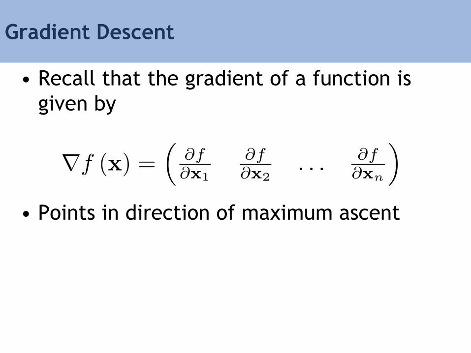
Gradient Descent
• Recall that the gradient of a function is
given by
• Points in direction of maximum ascent

An Aside: Level Sets
Level Set
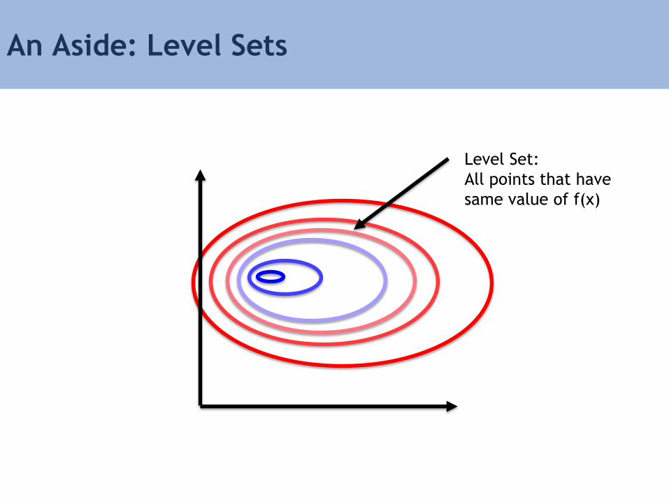
An Aside: Level Sets
Level Set:
All points that have
same value of f(x)

Gradient Descent

Gradient Descent
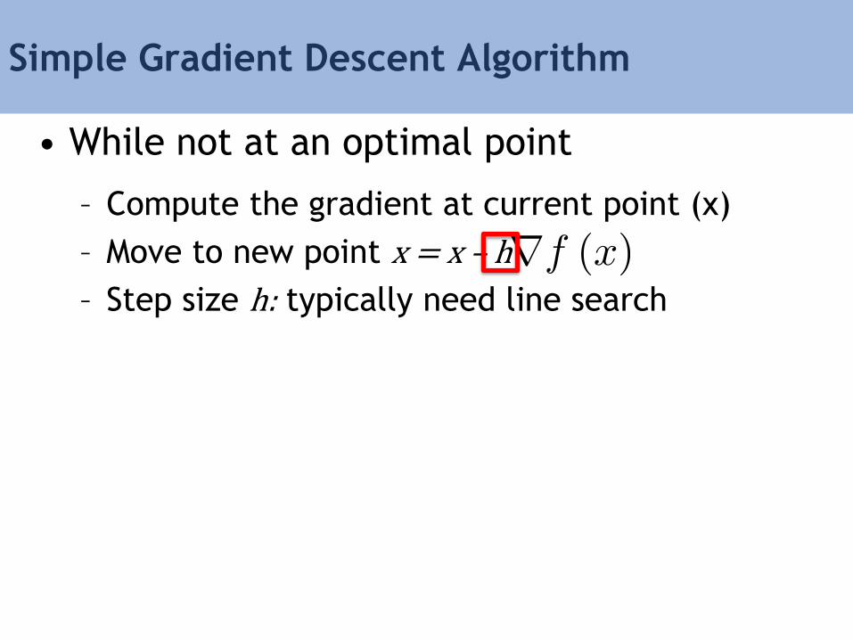
Simple Gradient Descent Algorithm
• While not at an optimal point
– Compute the gradient at current point (x)
– Move to new point x = x – h
– Step size h: typically need line search

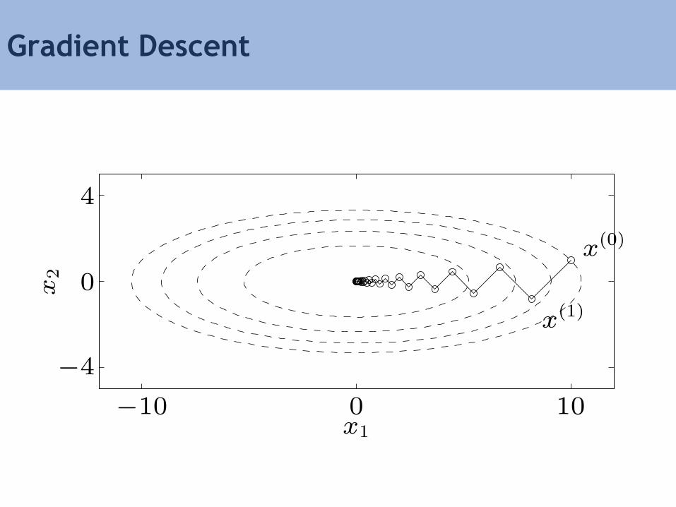
Gradient Descent

Gradient Descent
• Good:
– Simple to implement
• Bad:
– Sometimes converges badly
Gradient Descent
Newton’s Method
• Can we choose better search directions?
• Hint: quadratic functions are very nice!
A Simple Example: Least Squares
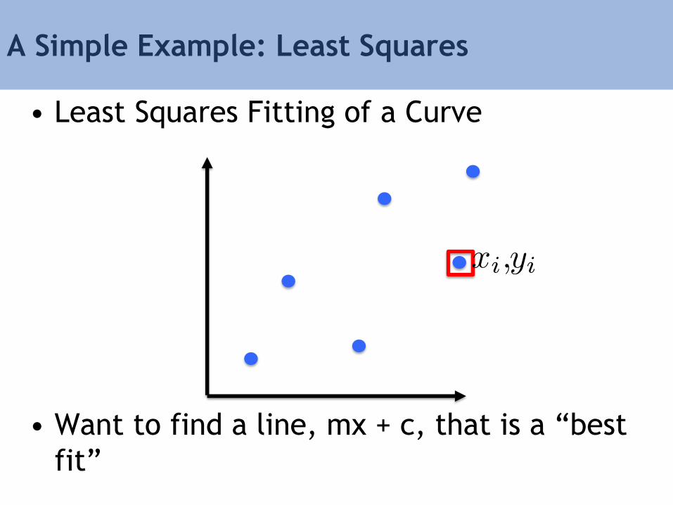
• Least Squares Fitting of a Curve
• Want to find a line, mx + c, that is a “best
fit”
A Simple Example: Least Squares
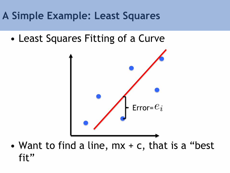
• Least Squares Fitting of a Curve
• Want to find a line, mx + c, that is a “best
fit”
Error=

A Simple Example: Least Squares
• Least Squares Fitting of a Curve
Error=
=
A Simple Example: Least Squares
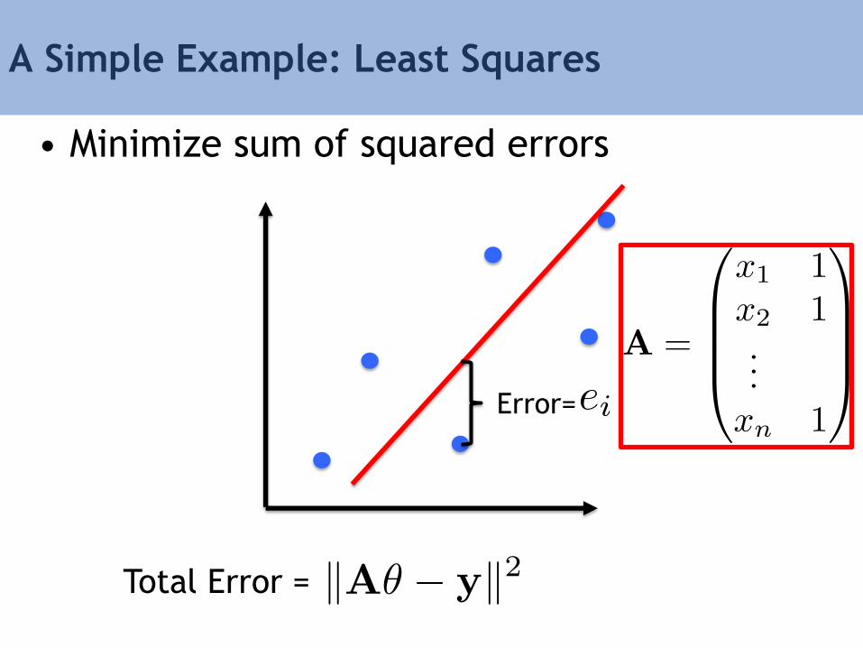
• Minimize sum of squared errors
Error=
Total Error =
A Simple Example: Least Squares
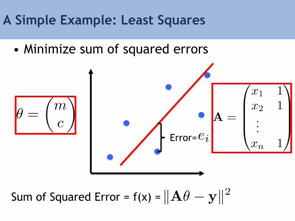
• Minimize sum of squared errors
Error=
Sum of Squared Error = f(x) =
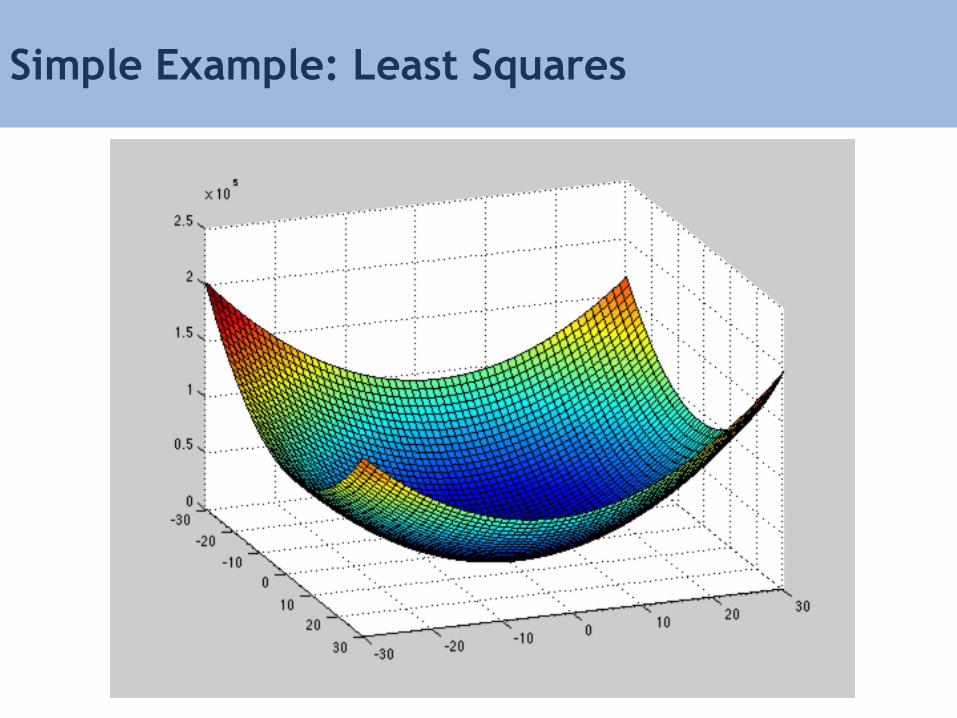
Simple Example: Least Squares

A Simple Example: Least Squares
• Solution given by the normal equations
Error=
Solution =
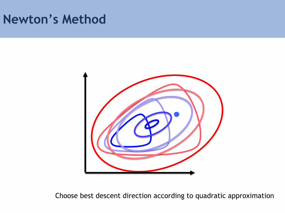
Newton’s Method
s s
Choose best descent direction according to quadratic approximation
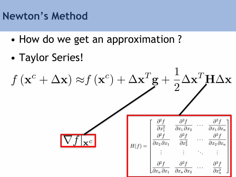
Newton’s Method
• How do we get an approximation ?
• Taylor Series!
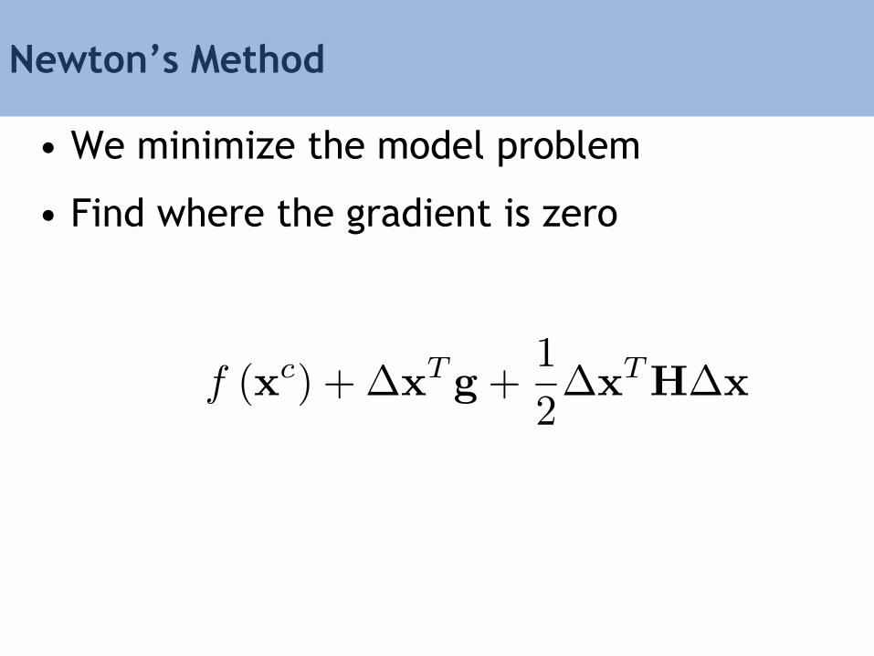
Newton’s Method
• We minimize the model problem
• Find where the gradient is zero

Newton’s Method
• We minimize the model problem
• Find where the gradient is zero
Model:
Gradient:
Increment:
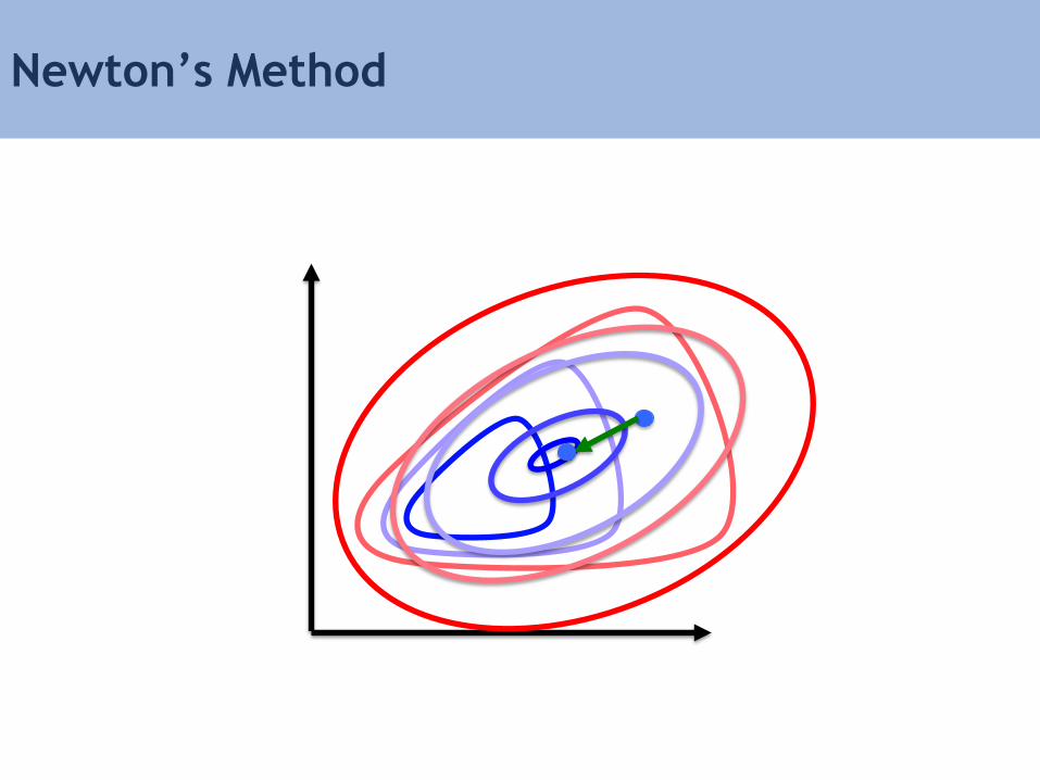
Newton’s Method
s s
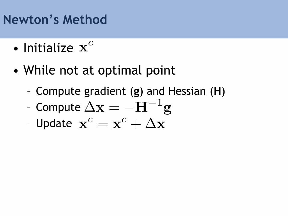
Newton’s Method
• Initialize
• While not at optimal point
– Compute gradient (g) and Hessian (H)
– Compute
– Update
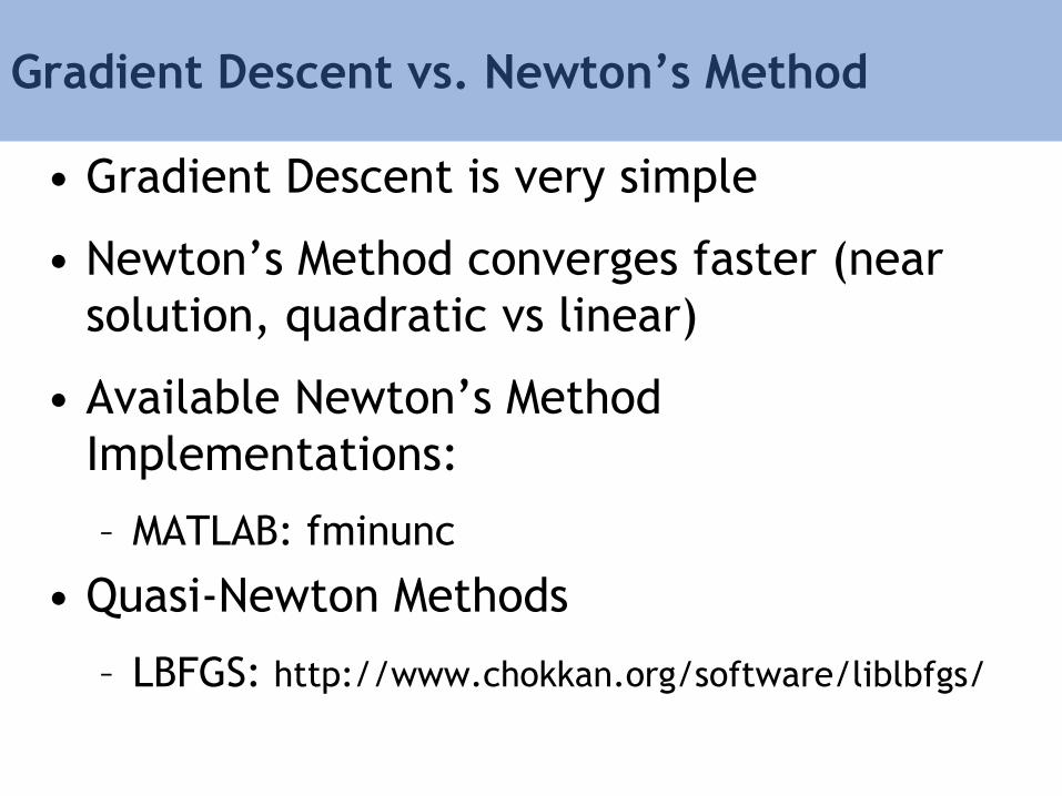
Gradient Descent vs. Newton’s Method
• Gradient Descent is very simple
• Newton’s Method converges faster (near
solution, quadratic vs linear)
• Available Newton’s Method
Implementations:
– MATLAB: fminunc
• Quasi-Newton Methods
– LBFGS: http://www.chokkan.org/software/liblbfgs/
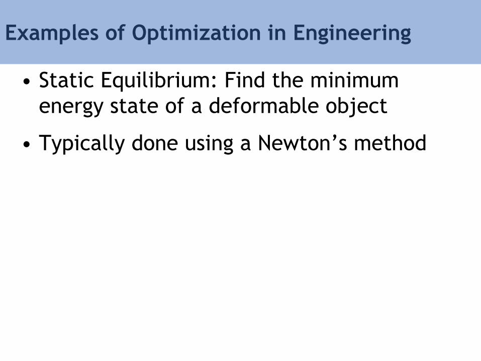
Examples of Optimization in Engineering
• Static Equilibrium: Find the minimum
energy state of a deformable object
• Typically done using a Newton’s method

Examples from Engineering
Types of Optimization
• Continuous vs. Discrete
• Constrained vs. Unconstrained
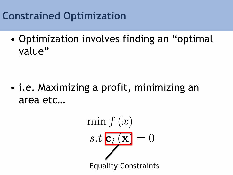
Constrained Optimization
• Optimization involves finding an “optimal
value”
• i.e. Maximizing a profit, minimizing an
area etc…
Equality Constraints
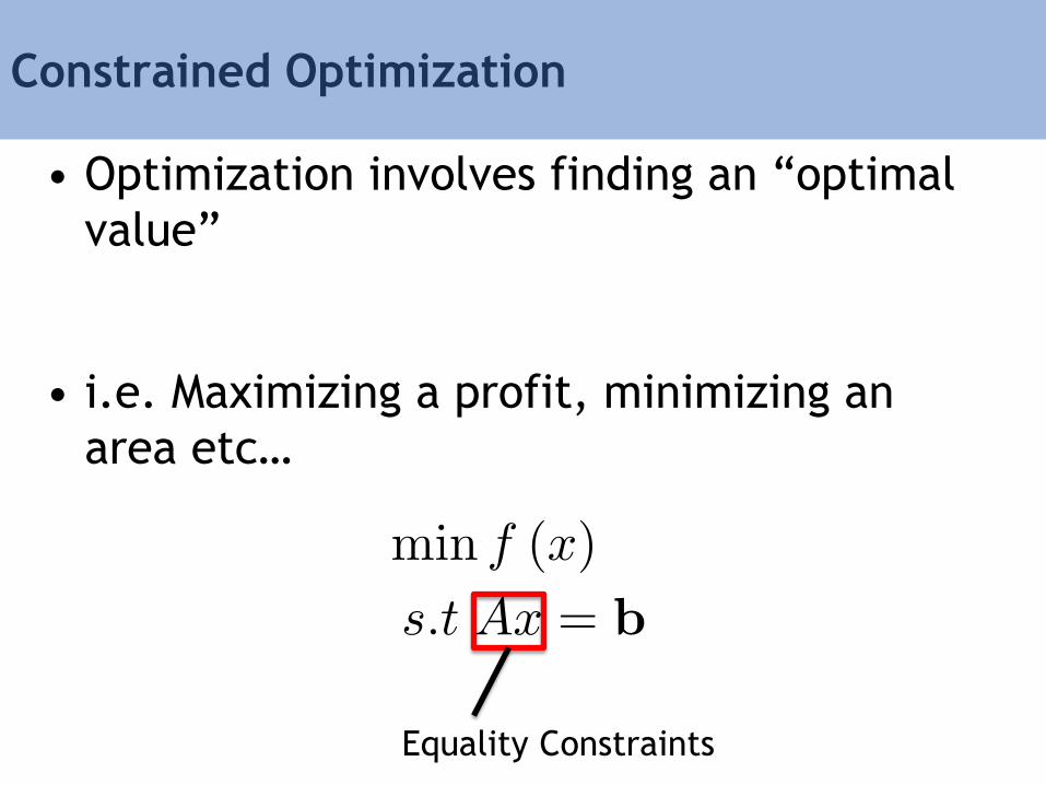
Constrained Optimization
• Optimization involves finding an “optimal
value”
• i.e. Maximizing a profit, minimizing an
area etc…
Equality Constraints

Constrained Optimization
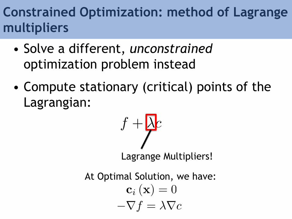
Constrained Optimization: method of Lagrange
multipliers
• Solve a different, unconstrained
optimization problem instead
• Compute stationary (critical) points of the
Lagrangian:
Lagrange Multipliers!
At Optimal Solution, we have:
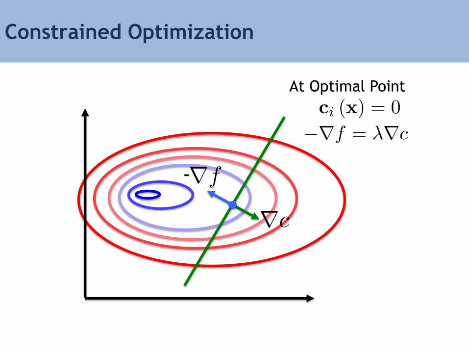
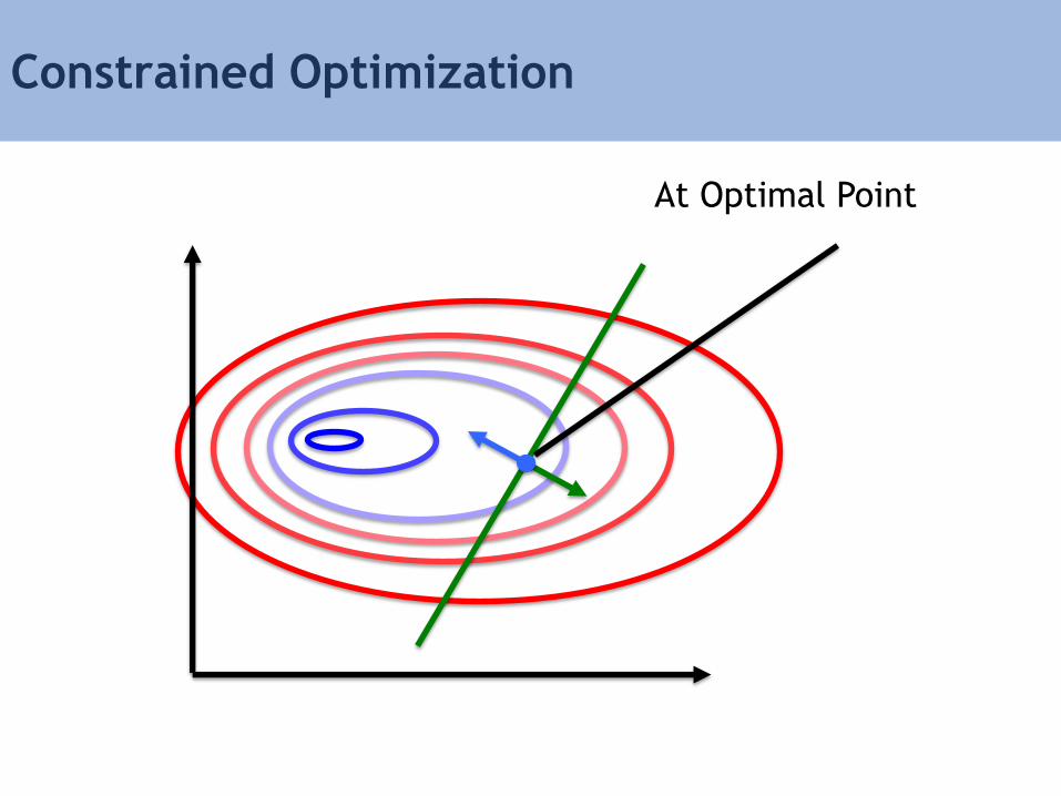
Constrained Optimization
At Optimal Point
-
Constrained Optimization
• Very useful for general equality
constrained problems
• Available in MATLAB as fmincon
• Easy to modify unconstrained Newton Code
Next: Inequality Constrained Optimization
• Specifically we will work up to a particular
type of problem called a Quadratic
Program
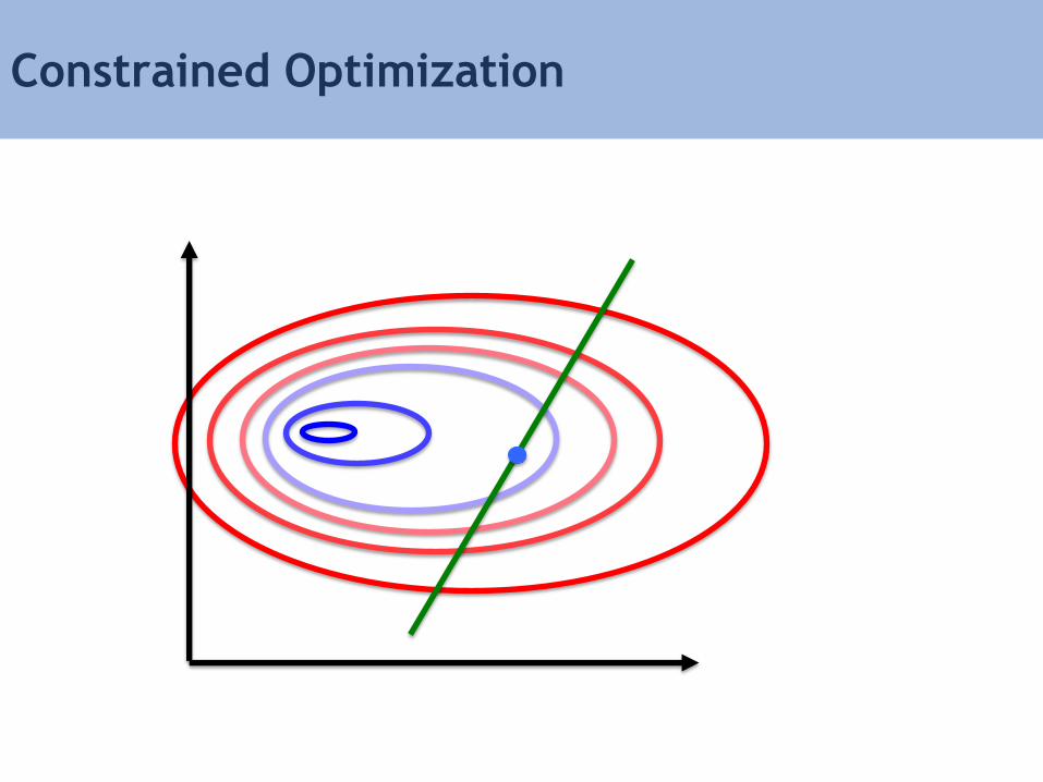
Constrained Optimization
Constrained Optimization
At Optimal Point
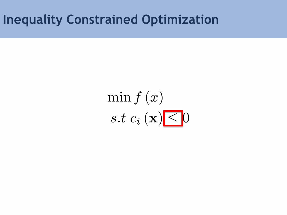
Inequality Constrained Optimization

Equality Constrained Optimization

Inequality Constrained Optimization
Feasible Set
The Active Set
• Hidden inside of each inequality
constrained optimization is an equality
constrained optimization
• There are two cases for our optimal point…
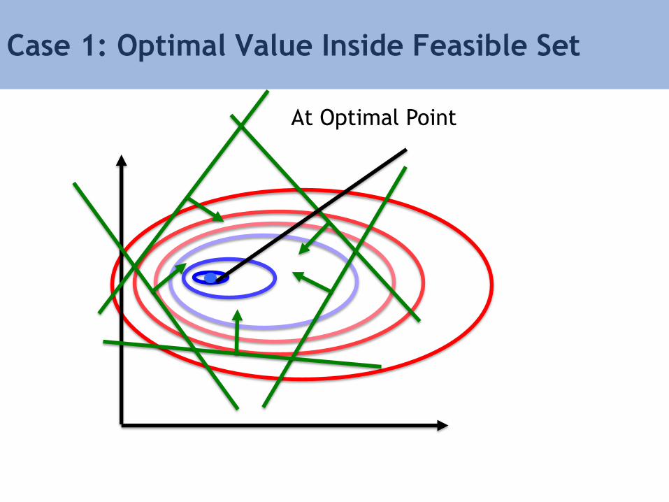
Case 1: Optimal Value Inside Feasible Set
At Optimal Point

Case 2: Optimal Value On Boundary
At Optimal Point
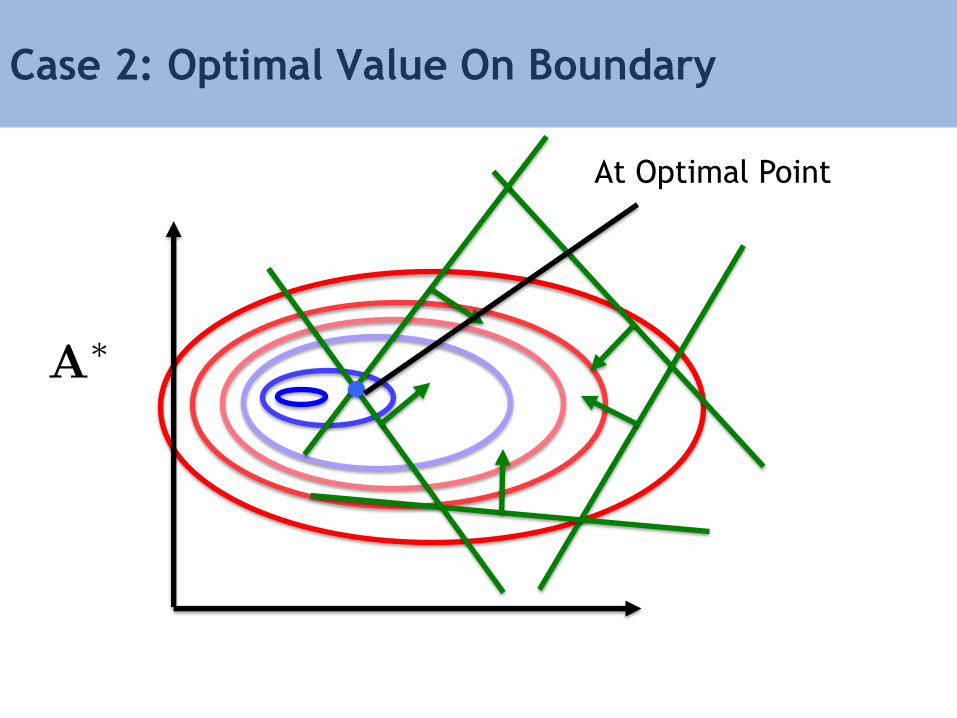
Case 2: Optimal Value On Boundary
At Optimal Point
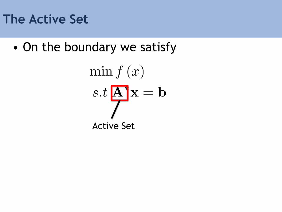
The Active Set
• On the boundary we satisfy
Active Set
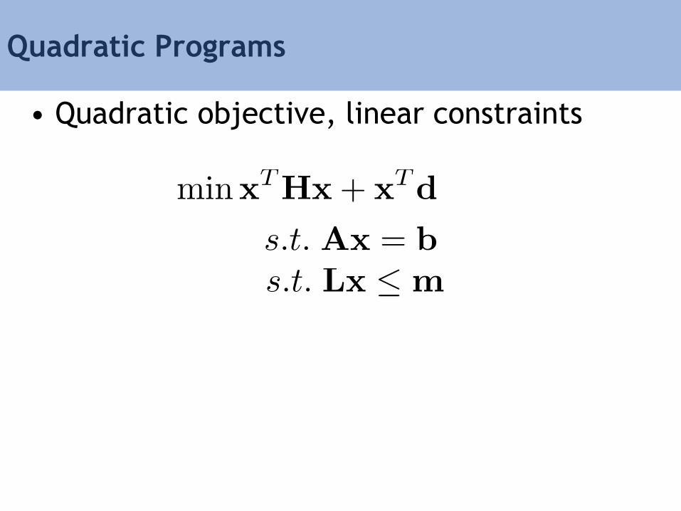
Quadratic Programs
• Quadratic objective, linear constraints
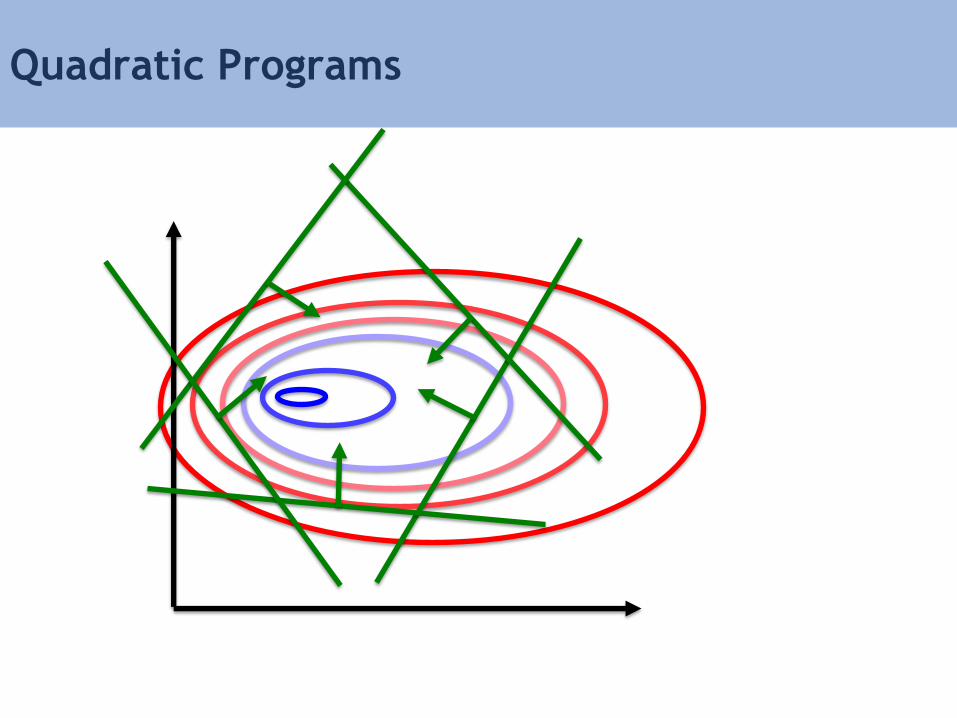
Quadratic Programs
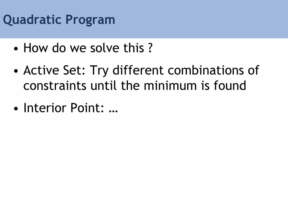
Quadratic Program
• How do we solve this ?
• Active Set: Try different combinations of
constraints until the minimum is found
• Interior Point: …
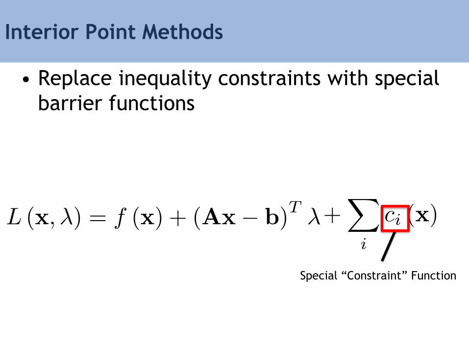
• Replace inequality constraints with special
barrier functions
Interior Point Methods
Special “Constraint” Function
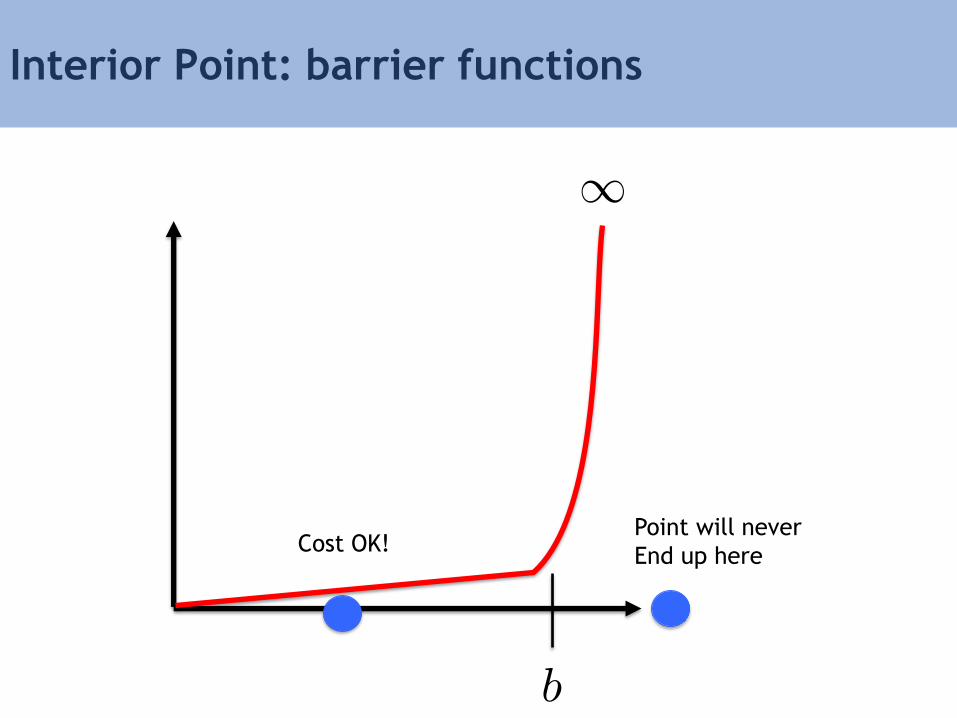
Interior Point: barrier functions
Cost OK! Point will never
End up here
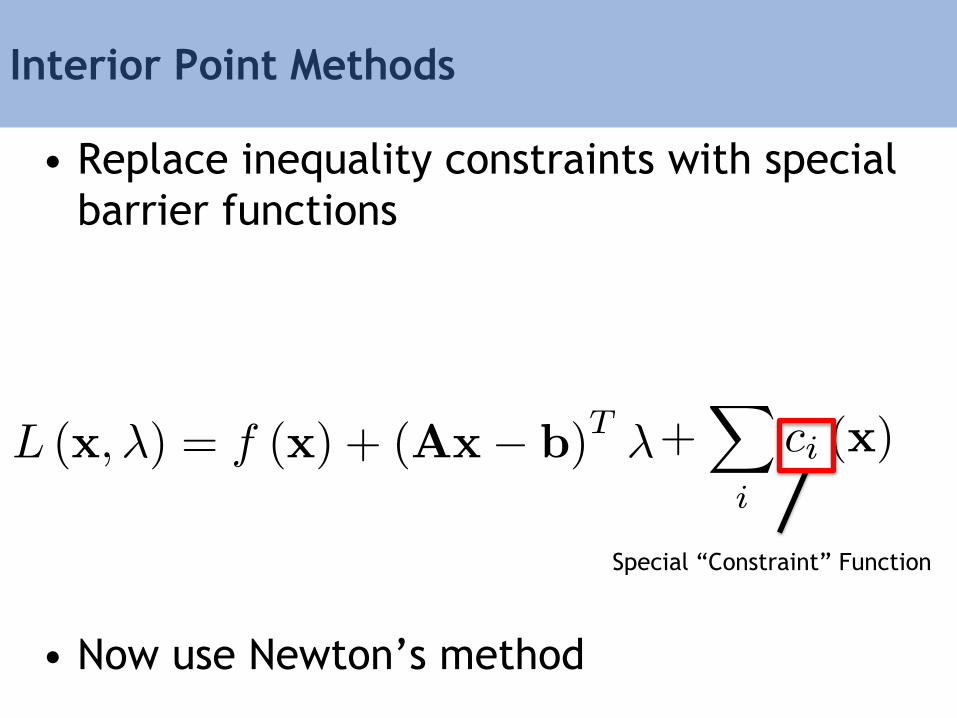
• Replace inequality constraints with special
barrier functions
• Now use Newton’s method
Interior Point Methods
Special “Constraint” Function

Quadratic Programs and Interior Point
• Quadratic Programs (Active Set)
– Quadprog++
(http://quadprog.sourceforge.net)
– MATLAB: quadprog
• Interior Point
– Ipopt (https://projects.coin-or.org/Ipopt)
Types of Optimization
• Continuous vs. Discrete
• Constrained vs. Unconstrained

Continuous Discrete
This point can move
smoothly
Choose from discrete points in
parameter space
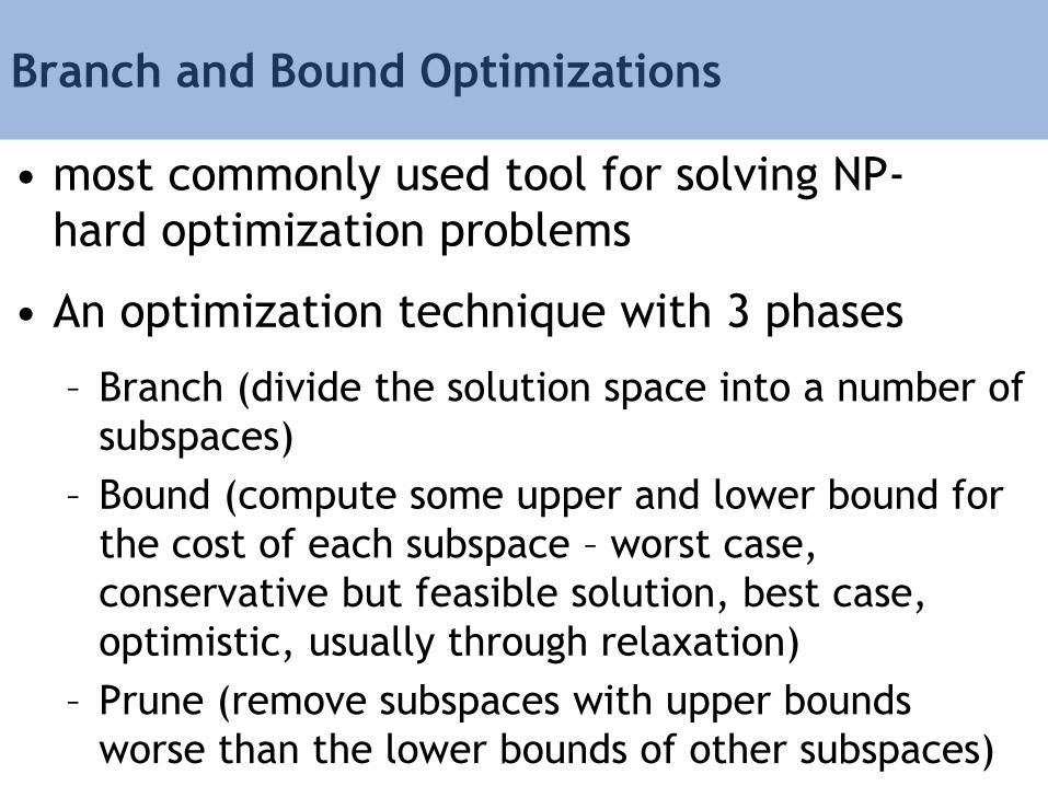
Branch and Bound Optimizations
• most commonly used tool for solving NP-
hard optimization problems
• An optimization technique with 3 phases
– Branch (divide the solution space into a number of
subspaces)
– Bound (compute some upper and lower bound for
the cost of each subspace – worst case,
conservative but feasible solution, best case,
optimistic, usually through relaxation)
– Prune (remove subspaces with upper bounds
worse than the lower bounds of other subspaces)
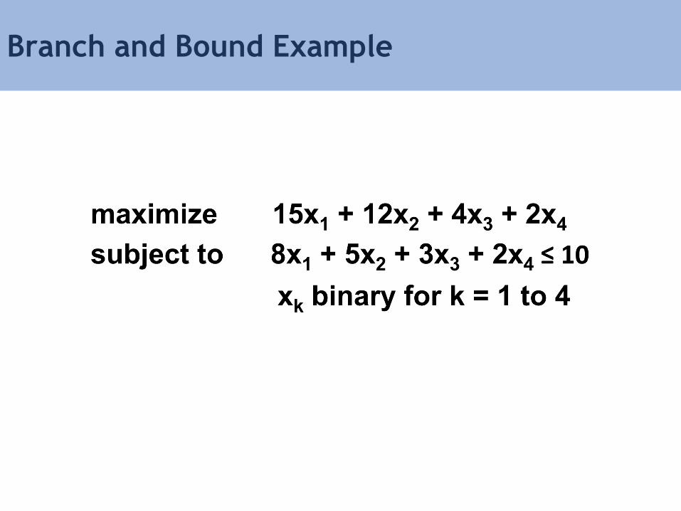
Branch and Bound Example

Branch and Bound Example
Enumerating all solutions is not feasible – exponential explosion
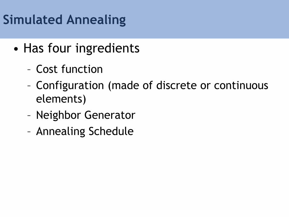
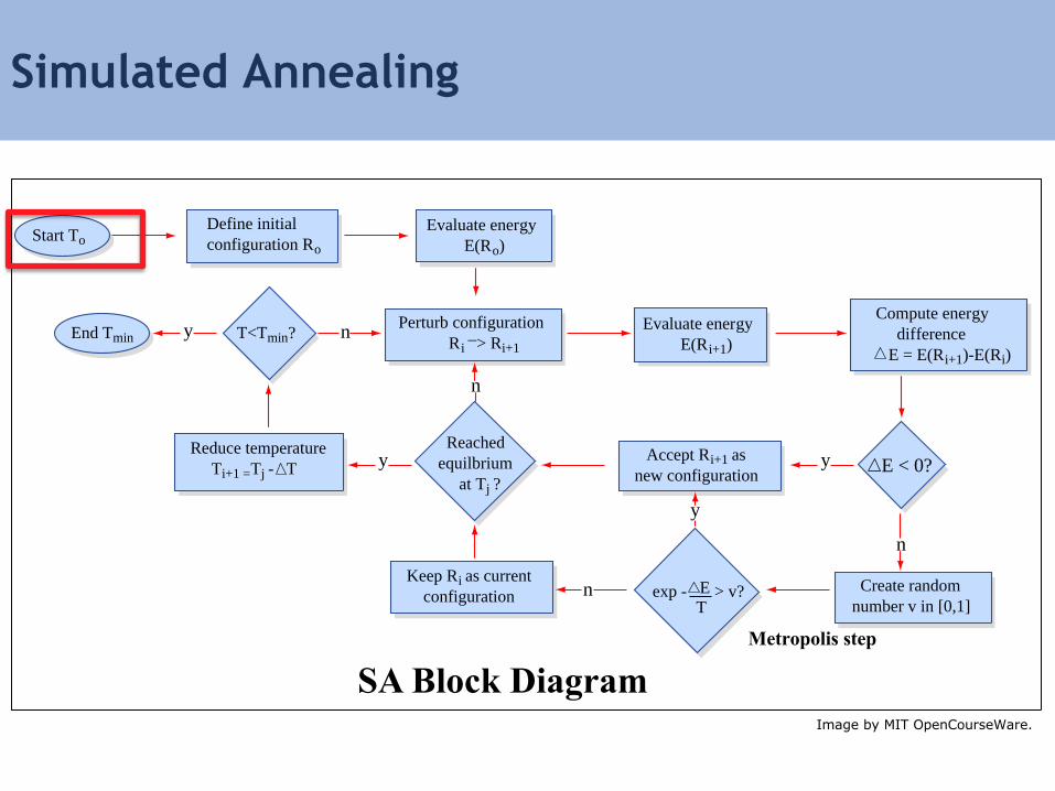
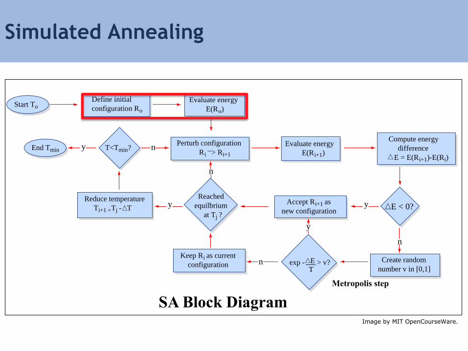
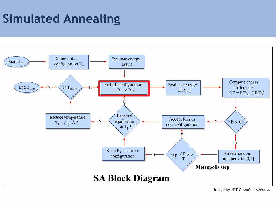
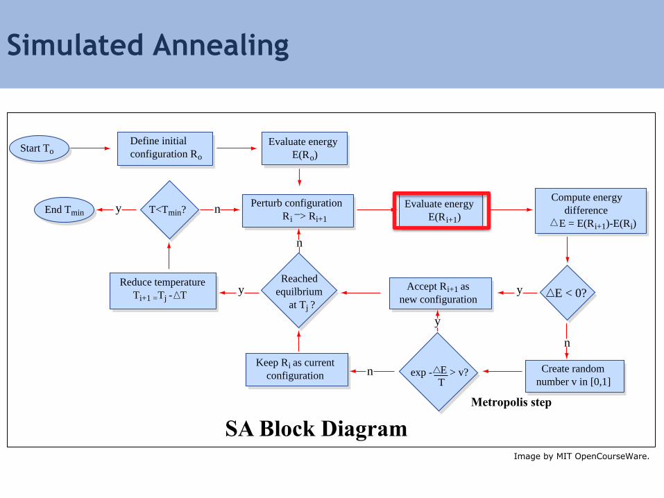
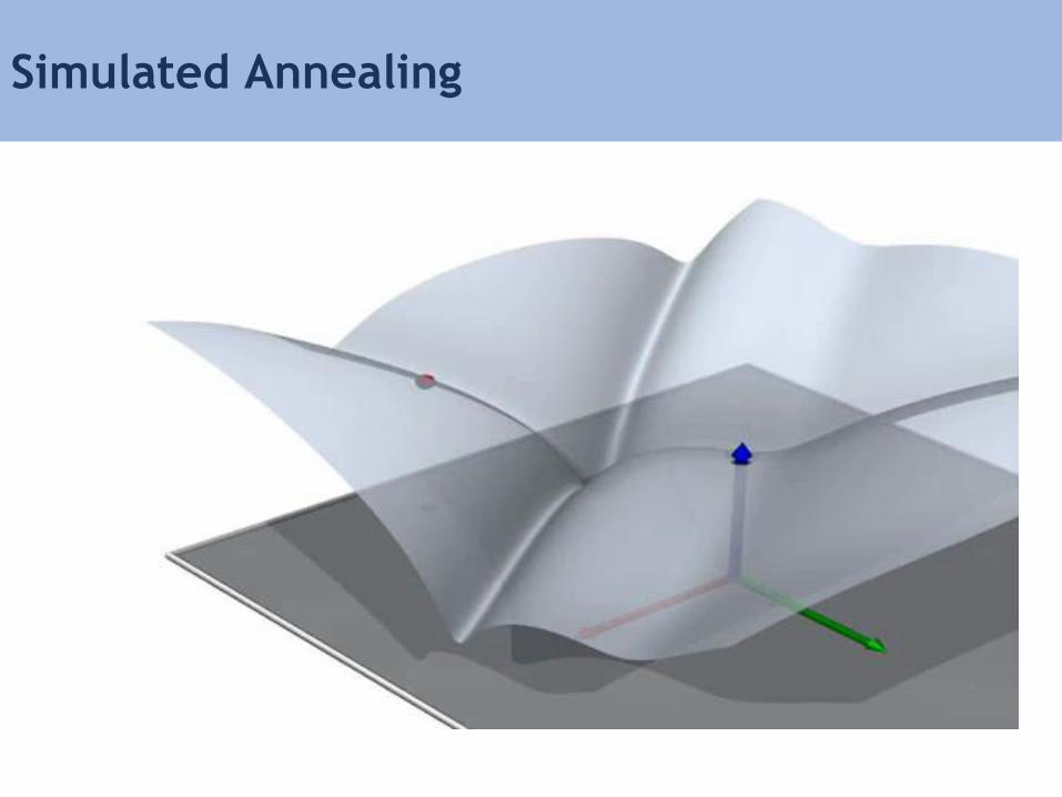
Simulated Annealing
• Has four ingredients
– Cost function
– Configuration (made of discrete or continuous
elements)
– Neighbor Generator
– Annealing Schedule
Simulated Annealing
• Basic Idea taken from cooling of materials
in metallurgy
• At high “heat” atoms undergo rigorous
motion
• As they are cooled they move less
• Explore trade-off between exploration and
exploitation
Simulated Annealing
• Cost function:
Simulated Annealing
• Cost function:
• Neighbor Generator: Rearrange Configuration
– Change q to something nearby
• Annealing Schedule
Simulated Annealing
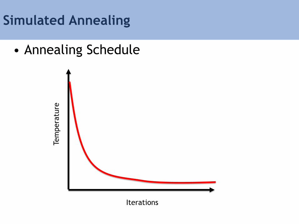
• Annealing Schedule Te
mpera
ture
Iterations
Simulated Annealing
27
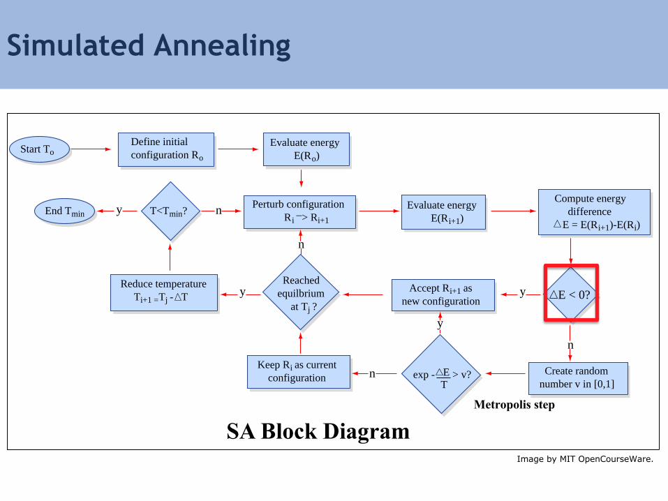
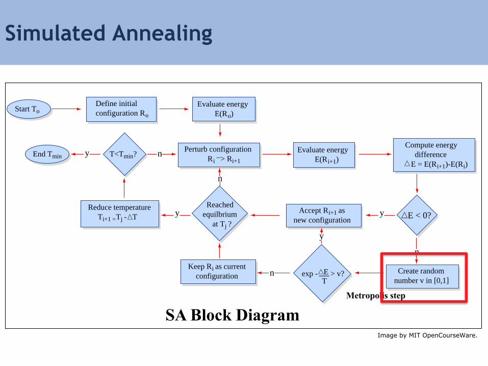
SA Block Diagram
n
Reached
equilbrium
at Tj ?
End Tmin
Start To
T<Tmin?
Define initial
configuration Ro
Evaluate energy
E(Ro)
Evaluate energy
E(Ri+1)
Accept Ri+1 as
new configuration
Keep Ri as current
configuration
Perturb configuration
Ri _
> Ri+1
Compute energy
difference
E = E(Ri+1)-E(Ri)
Reduce temperature
Ti+1 =Tj - T E < 0?
Create random
number v in [0,1]exp - E > v?
T
Metropolis step
SA Block Diagram
y
y
y
n
n
n
y
Image by MIT OpenCourseWare.
Simulated Annealing
27
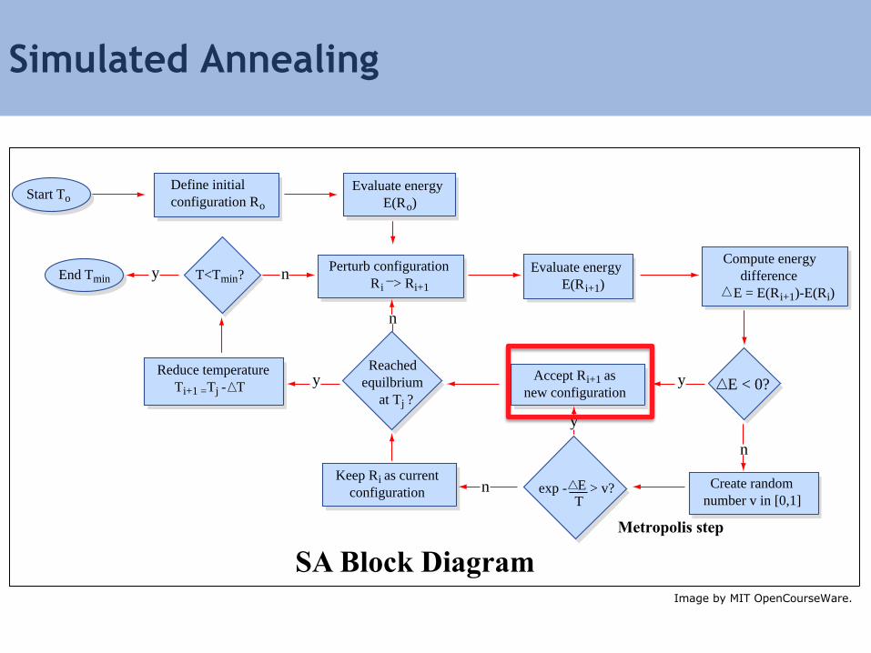
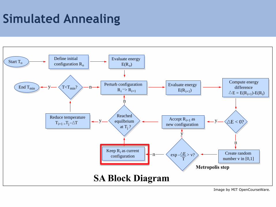
SA Block Diagram
n
Reached
equilbrium
at Tj ?
End Tmin
Start To
T<Tmin?
Define initial
configuration Ro
Evaluate energy
E(Ro)
Evaluate energy
E(Ri+1)
Accept Ri+1 as
new configuration
Keep Ri as current
configuration
Perturb configuration
Ri _
> Ri+1
Compute energy
difference
E = E(Ri+1)-E(Ri)
Reduce temperature
Ti+1 =Tj - T E < 0?
Create random
number v in [0,1]exp - E > v?
T
Metropolis step
SA Block Diagram
y
y
y
n
n
n
y
Image by MIT OpenCourseWare.
Simulated Annealing
27
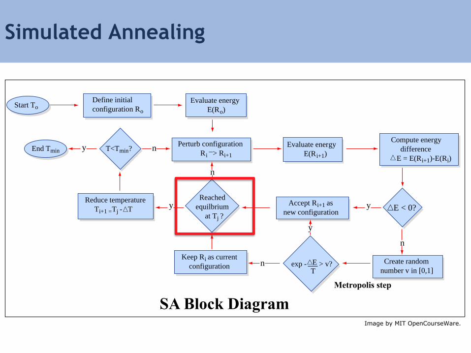
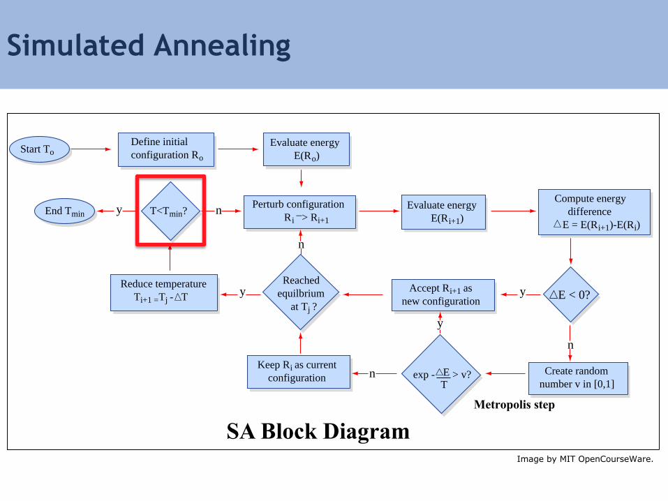
SA Block Diagram
n
Reached
equilbrium
at Tj ?
End Tmin
Start To
T<Tmin?
Define initial
configuration Ro
Evaluate energy
E(Ro)
Evaluate energy
E(Ri+1)
Accept Ri+1 as
new configuration
Keep Ri as current
configuration
Perturb configuration
Ri _
> Ri+1
Compute energy
difference
E = E(Ri+1)-E(Ri)
Reduce temperature
Ti+1 =Tj - T E < 0?
Create random
number v in [0,1]exp - E > v?
T
Metropolis step
SA Block Diagram
y
y
y
n
n
n
y
Image by MIT OpenCourseWare.
Simulated Annealing
27
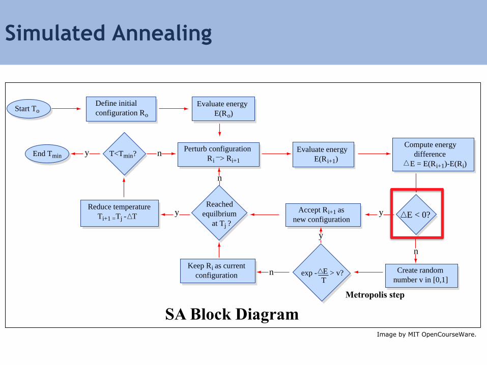
SA Block Diagram
n
Reached
equilbrium
at Tj ?
End Tmin
Start To
T<Tmin?
Define initial
configuration Ro
Evaluate energy
E(Ro)
Evaluate energy
E(Ri+1)
Accept Ri+1 as
new configuration
Keep Ri as current
configuration
Perturb configuration
Ri _
> Ri+1
Compute energy
difference
E = E(Ri+1)-E(Ri)
Reduce temperature
Ti+1 =Tj - T E < 0?
Create random
number v in [0,1]exp - E > v?
T
Metropolis step
SA Block Diagram
y
y
y
n
n
n
y
Image by MIT OpenCourseWare.

Simulated Annealing
27
SA Block Diagram
n
Reached
equilbrium
at Tj ?
End Tmin
Start To
T<Tmin?
Define initial
configuration Ro
Evaluate energy
E(Ro)
Evaluate energy
E(Ri+1)
Accept Ri+1 as
new configuration
Keep Ri as current
configuration
Perturb configuration
Ri _
> Ri+1
Compute energy
difference
E = E(Ri+1)-E(Ri)
Reduce temperature
Ti+1 =Tj - T E < 0?
Create random
number v in [0,1]exp - E > v?
T
Metropolis step
SA Block Diagram
y
y
y
n
n
n
y
Image by MIT OpenCourseWare.
Simulated Annealing
• Global optimization
• Combinatorial optimization
• Difficult to define good annealing schedule
and neighbor generation scheme
Simulated Annealing

Examples from Graphics