Embed Size (px)
Citation preview

An Introduction toObjective Bayesian Statistics
Jose M. Bernardo
Universitat de Valencia, Spain
XXVI Winter School of Astrophysics
Tenerife (Islas Canarias, Spain), November, 2014
Objective Bayesian Statistics 2
(i) Concept of Probability
• Introduction. Notation. Statistical models.
• Intrinsic discrepancy. Intrinsic convergence of distributions.
• Foundations. Probability as a rational degree of belief.
(ii) Basics of Bayesian Analysis
• Parametric inference. The learning process.
• Reference analysis. No relevant initial information.
• Inference summaries. Point and region estimation.
• Prediction. Regression.
• Hierarchical models. Exchangeability.
Objective Bayesian Statistics 3
(iii) Integrated Reference Analysis
• Structure of a decision problem. Axiomatics.
• Decision structure of inference summaries. Estimation and
Hypothesis testing.
• Loss functions in inference problems. The intrinsic discrep-
ancy loss.
• Objective Bayesian methods. Reference priors.
• An integrated approach to objective Bayesian inference. In-
trinsic posterior analysis.
(iv) Basic References
Objective Bayesian Statistics 4
Concept of Probability
Introduction
• One tentatively accepts a formal statistical model, typically sug-
gested by informal descriptive evaluation.
Conclusions are obviously conditional on the assumption that the
model is correct.
• The Bayesian approach is firmly based on axiomatic foundations.
These imply that all uncertainties must be described by probabilities.
• In particular, parameters must have a (prior) distribution describing
available information about their values.
This is not a description of their variability (since they are fixed
unknown quantities), but a description of the uncertainty about their
true values.
Objective Bayesian Statistics 5
• An important particular case arises when there is no relevant ob-
jective initial information, and the use of subjective information is
not desired.
This typically occurs in scientific and industrial reporting, public
decision making, auditing, and many other situations
• Bayesian analysis then requires a prior distributions exclusively based
on model assumptions and available, well-documented data.
This is the subject of Objective Bayesian Statistics.
Objective Bayesian Statistics 6
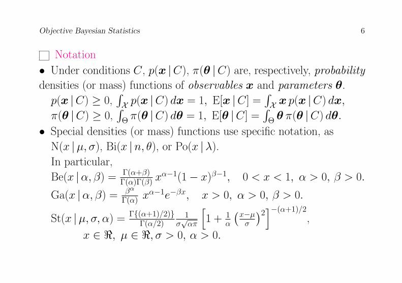
Notation
• Under conditions C, p(x |C), π(θ |C) are, respectively, probability
densities (or mass) functions of observables x and parameters θ.
p(x |C) ≥ 0,∫X p(x |C) dx = 1, E[x |C] =
∫X x p(x |C) dx,
π(θ |C) ≥ 0,∫
Θ π(θ |C) dθ = 1, E[θ |C] =∫
Θ θ π(θ |C) dθ.
• Special densities (or mass) functions use specific notation, as
N(x |µ, σ), Bi(x |n, θ), or Po(x |λ).
In particular,
Be(x |α, β) = Γ(α+β)Γ(α)Γ(β) x
α−1(1− x)β−1, 0 < x < 1, α > 0, β > 0.
Ga(x |α, β) = βα
Γ(α) xα−1e−βx, x > 0, α > 0, β > 0.
St(x |µ, σ, α) = Γ(α+1)/2)Γ(α/2)
1σ√απ
[1 + 1
α
(x−µσ
)2]−(α+1)/2
,
x ∈ <, µ ∈ <, σ > 0, α > 0.
Objective Bayesian Statistics 7
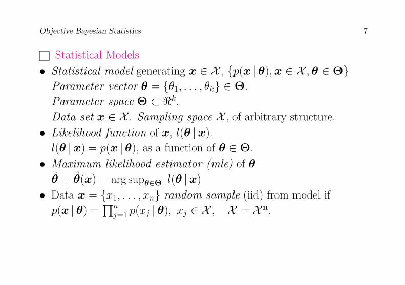
Statistical Models
• Statistical model generating x ∈ X , p(x |θ),x ∈ X ,θ ∈ ΘParameter vector θ = θ1, . . . , θk ∈ Θ.
Parameter space Θ ⊂ <k.Data set x ∈ X . Sampling space X , of arbitrary structure.
• Likelihood function of x, l(θ |x).
l(θ |x) = p(x |θ), as a function of θ ∈ Θ.
• Maximum likelihood estimator (mle) of θ
θ = θ(x) = arg supθ∈Θ l(θ |x)
• Data x = x1, . . . , xn random sample (iid) from model if
p(x |θ) =∏n
j=1 p(xj |θ), xj ∈ X , X = X n.
Objective Bayesian Statistics 8
• Behaviour under repeated sampling (general, not necessarily iid data)
is obtained by considering x1,x2, . . ., a (possibly infinite) sequence
of possible replications of the complete data set x.
Denote by x(m) = x1, . . . ,xm a finite set of m such replications.
Asymptotic results are obtained as m→∞.
• Data x1, . . . ,xn are often assumed to be exchangeable in that
their joint distribution p(x1, . . . ,xn) may be considered to be invariant
under permutations (order of observation inmaterial)
• Under exchangeability, parameters may formally be definedas asymp-
totic limits of specific data functions.
Thus, If data x1, . . . , xn are exchangeable 0-1 random quantities,
then p(xi) = θxi(1 − θ)1−xi, with θ = limm→∞(1/m)∑m
i=1 xi. Or, if
data x1, . . . ,xn are exchangeable normal vectors N(xi |µ,Σ), then
µ = limm→∞(1/m)∑m
i=1xi.
Objective Bayesian Statistics 9
Intrinsic Divergence
Logarithmic divergences
• The logarithmic divergence (Kullback-Leibler) kp | p of a density
p(x), x ∈ X from its true density p(x), is
κp | p =∫X p(x) log p(x)
p(x) dx, (provided this exists)
• The functional κp | p is non-negative; it is zero iff p(x) = p(x)
(a.e.), and it is invariant under one-to-one transformations of x.
• But κp1 | p2 is not symmetric and diverges if, strictly, X2 ⊂ X1 .
Intrinsic discrepancy between distributions
• δp1, p2 = min∫X1
p1(x) log p1(x)p2(x) dx,
∫X2
p2(x) log p2(x)p1(x) dx
The intrinsic discrepancy δp1, p2 is non-negative; it is zero iff,
p1 = p2 a.e., and it is invariant under one-to-one transformations
of x,
Objective Bayesian Statistics 10
• The intrinsic discrepancy is defined even if either X2 ⊂ X1 or
X1 ⊂ X2. It has an operative interpretation as the minimum amount
of information (in nits) required to discriminate between the two dis-
tributions.
Interpretation of the intrinsic discrepancy
• Let p1(x |θ1),θ1 ∈ Θ1 or p2(x |θ2),θ2 ∈ Θ2 be two alter-
native statistical models for x ∈ X , one of which is assumed to be
true. The intrinsic divergence δθ1,θ2 = δp1, p2 is then minimum
expected log-likelihood ratio in favour of the true model.
Indeed, if p1(x |θ1) true model, the expected log-likelihood ratio in
its favour is E1[logp1(x |θ1)/p2(x |θ1)] = κp2 | p1. If the true
model is p2(x |θ2), the expected log-likelihood ratio in favour of the
true model is κp2 | p1. But δp2 | p1 = min[κp2 | p1, κp1 | p2].
Objective Bayesian Statistics 11
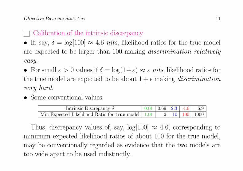
Calibration of the intrinsic discrepancy
• If, say, δ = log[100] ≈ 4.6 nits, likelihood ratios for the true model
are expected to be larger than 100 making discrimination relatively
easy.
• For small ε > 0 values if δ = log(1+ε) ≈ ε nits, likelihood ratios for
the true model are expected to be about 1 + ε making discrimination
very hard.
• Some conventional values:
Intrinsic Discrepancy δ 0.01 0.69 2.3 4.6 6.9Min Expected Likelihood Ratio for true model 1.01 2 10 100 1000
Thus, discrepancy values of, say, log[100] ≈ 4.6, corresponding to
minimum expected likelihood ratios of about 100 for the true model,
may be conventionally regarded as evidence that the two models are
too wide apart to be used indistinctly.
Objective Bayesian Statistics 12
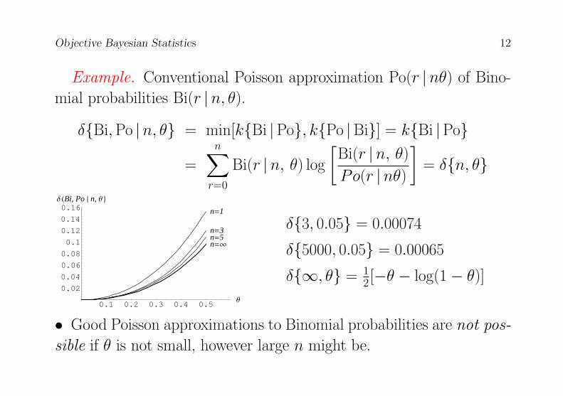
Example. Conventional Poisson approximation Po(r |nθ) of Bino-
mial probabilities Bi(r |n, θ).
δBi,Po |n, θ = min[kBi |Po, kPo |Bi] = kBi |Po
=
n∑r=0
Bi(r |n, θ) log
[Bi(r |n, θ)
Po(r |nθ)
]= δn, θ
0.1 0.2 0.3 0.4 0.5Θ
0.02
0.04
0.06
0.08
0.1
0.12
0.14
0.16∆ HBi, Po È n, Θ <
n=1
n=3n=5n=¥
δ3, 0.05 = 0.00074
δ5000, 0.05 = 0.00065
δ∞, θ = 12[−θ − log(1− θ)]
• Good Poisson approximations to Binomial probabilities are not pos-
sible if θ is not small, however large n might be.
Objective Bayesian Statistics 13
Intrinsic Convergence of Distributions
• Intrinsic convergence. A sequence of probability densities (or mass)
functions pi(x)∞i=1 converges intrinsically to p(x) if (and only if) the
intrinsic divergence between pi(x) and p(x) converges to zero. i.e., iff
limi→∞ δ(pi, p) = 0.
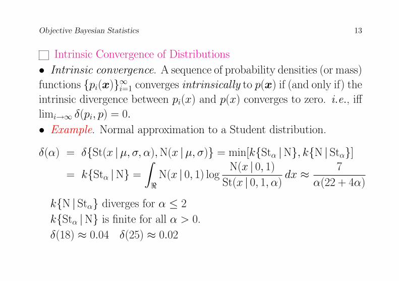
• Example. Normal approximation to a Student distribution.
δ(α) = δSt(x |µ, σ, α),N(x |µ, σ) = min[kStα |N, kN | Stα]
= kStα |N =
∫<
N(x | 0, 1) logN(x | 0, 1)
St(x | 0, 1, α)dx ≈ 7
α(22 + 4α)
kN | Stα diverges for α ≤ 2
kStα |N is finite for all α > 0.
δ(18) ≈ 0.04 δ(25) ≈ 0.02
Objective Bayesian Statistics 14
20 40 60 80 100
0.002
0.004
0.006
0.008
0.01
Α
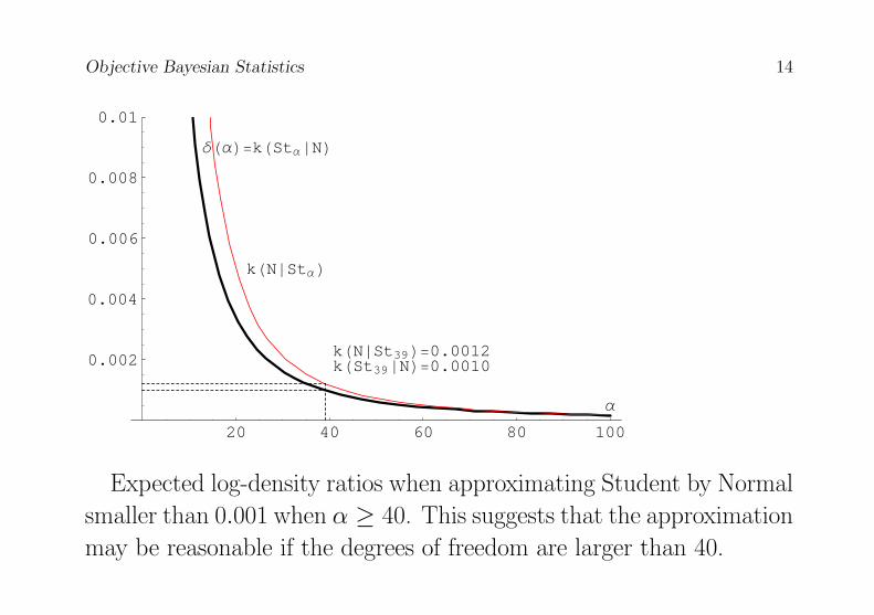
kHNÈStΑL
∆HΑL=kHStΑÈNL
kHNÈSt39L=0.0012kHSt39ÈNL=0.0010
Expected log-density ratios when approximating Student by Normal
smaller than 0.001 when α ≥ 40. This suggests that the approximation
may be reasonable if the degrees of freedom are larger than 40.
Objective Bayesian Statistics 15
Foundations
Foundations of Statistics
• Axiomatic foundations on rational description of uncertainty imply
that the uncertainty about all unknown quantities should be measured
with probability distributions π(θ |C),θ ∈ Θ describing their plau-
sibility given available conditions C.
• Axioms have a strong intuitive appeal; examples include:
• Transitivity of plausibility
If E1 > E2 |C, and E2 > E3 |C, then E1 > E3 |C• The sure-thing principle
If E1 > E2 |A,C and E1 > E2 |A,C, then E1 > E2 |C).
• Axioms are not a description of actual human activity, but a nor-
mative set of principles for those aspiring to rational behaviour.
Objective Bayesian Statistics 16
• “Absolute” probabilities do not exist. Typical applications produce
Pr(E |x, A,K), a measure of rational belief in the occurrence of the
event E, given data x, assumptions A and available knowledge K.
Probability as a Measure of Conditional Uncertainty
• Axiomatic foundations imply that Pr(E |C), the probability of an
event E given C is always a conditional measure of the (presumably
rational) uncertainty, on a [0, 1] scale, about the occurrence of E in
conditions C.
• Probabilistic diagnosis. V is the event that a person carries a virus
and + a positive test result. All related probabilities, e.g.,
Pr(+ |V ) = 0.98, Pr(+ |V ) = 0.01, Pr(V |K) = 0.002,
Pr(+ |K) = Pr(+ |V ) Pr(V |K) + Pr(+ |V ) Pr(V |K) = 0.012
Pr(V |+, A,K) = Pr(+ |V ) Pr(V |K)Pr(+ |K) = 0.164 (Bayes’ Theorem)
are conditional uncertainty measures (and proportion estimates).
Objective Bayesian Statistics 17
• Estimation of a proportion. Survey conducted to estimate
the proportion θ of positive individuals in a population.
Random sample of size n with r positive.
Pr(a < θ < b | r, n, A,K), a conditional measure of the uncertainty
about the event that θ belongs to [a, b] given assumptions A,
initial knowledge K and data r, n.• Measurement of a physical constant. Measuring the unknown
value of a physical constant µ, with data x = x1, . . . , xn, considered
to be measurements of µ subject to error.
Desired to find Pr(a < µ < b |x = x1, . . . , xn, A,K), the prob-
ability that the unknown value of µ (fixed in nature, but unknown to
the scientists) belongs to [a, b], given the information provided by the
data x, any assumptions A made, and available knowledge K.
Objective Bayesian Statistics 18
Nuisance parameters
• The statistical model usually include nuisance parameters, unknown
quantities , which have to be eliminated in the statement of the final
results.
For instance, the precision of the measurements described by un-
known standard deviation σ in a N(x |µ, σ) normal model.
Restrictions
• Relevant scientific information may impose restrictions on the ad-
missible values of the quantities of interest. These must be taken into
account.
For instance, in measuring the value of the gravitational field g in a
laboratory, it is known that it must lie between 9.7803 m/sec2 (average
value at the Equator) and 9.8322 m/sec2 (average value at the poles).
Objective Bayesian Statistics 19
• Future discrete observations. Counting the number r of times that
an event E takes place in each of n replications. Desired to forecast the
number of times r that E will take place in a future, similar situation,
Pr(r | r1, . . . , rn, A,K). For instance, no accidents in each of n = 10
consecutive months may yield Pr(r = 0 |x, A,K) = 0.953.
• Future continuous observations. Data x = y1, . . . ,yn. Desired
p(y |x, A,K), to forecast a future observation y. For instance, from
breaking strengths x = y1, . . . , yn of n randomly chosen safety belt
webbings, the engineer may find Pr(y > y∗ |x, A,K) = 0.9987.
• Regression. Data set consists of pairs x = (y1,v1), . . . , (yn,vn)of quantity yj observed in conditions vj. Desired to forecast the value
of y in conditions v, p(y |v,x, A,K). For instance, with y contam-
ination levels and v wind speed from source, environment authorities
may be interested in Pr(y > y∗ | v,x, A,K).
Objective Bayesian Statistics 20
Basics of Bayesian Analysis
Parametric Inference
Bayes Theorem
• Let M = p(x |θ),x ∈ X ,θ ∈ Θ be an statistical model, let
π(θ |K) be a probability density for θ given prior knowledge K and
let x be some available data.
π(θ |x,M,K) =p(x |θ) π(θ |K)∫
Θ p(x |θ) π(θ |K) dθ,
encapsulates all information about θ given data and prior knowledge.
• Simplifying notation, Bayes’ theorem may be expressed as
π(θ |x) ∝ p(x |θ) π(θ)
The posterior is proportional to the likelihood times the prior.
Objective Bayesian Statistics 21
• The missing proportionality constant in π(θ |x) ∝ p(x |θ) π(θ),
c(x) = [∫
Θ p(x |θ) π(θ) dθ]−1 may be deduced from the fact that
π(θ |x) must integrate to one. To identify a posterior distribution it
suffices to identify a kernel k(θ,x) such that π(θ |x) = c(x) k(θ,x).
This is a very common technique.
Bayesian Inference with a Finite Parameter Space
• Model p(x | θi),x ∈ X , θi ∈ Θ, with Θ = θ1, . . . , θm, so that θ
may only take a finite number m of different values. Using the finite
form of Bayes’ theorem,
Pr(θi |x) =p(x | θi) Pr(θi)∑mj=1 p(x | θj) Pr(θj)
, i = 1, . . . ,m.
Objective Bayesian Statistics 22
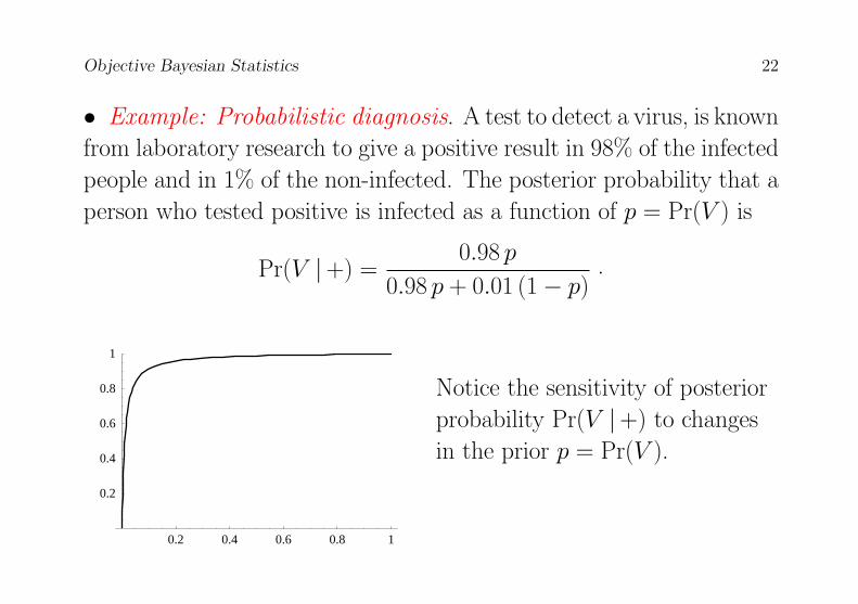
• Example: Probabilistic diagnosis. A test to detect a virus, is known
from laboratory research to give a positive result in 98% of the infected
people and in 1% of the non-infected. The posterior probability that a
person who tested positive is infected as a function of p = Pr(V ) is
Pr(V |+) =0.98 p
0.98 p + 0.01 (1− p).
0.2 0.4 0.6 0.8 1
0.2
0.4
0.6
0.8
1
Notice the sensitivity of posterior
probability Pr(V |+) to changes
in the prior p = Pr(V ).
Objective Bayesian Statistics 23
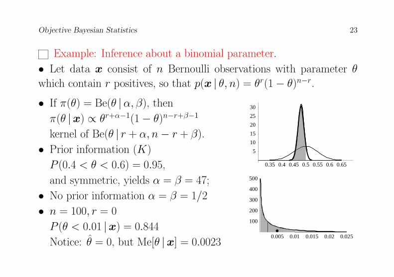
Example: Inference about a binomial parameter.
• Let data x consist of n Bernoulli observations with parameter θ
which contain r positives, so that p(x | θ, n) = θr(1− θ)n−r.
0.005 0.01 0.015 0.02 0.025
100
200
300
400
500
0.35 0.4 0.45 0.5 0.55 0.6 0.65
5
10
15
20
25
30• If π(θ) = Be(θ |α, β), then
π(θ |x) ∝ θr+α−1(1− θ)n−r+β−1
kernel of Be(θ | r + α, n− r + β).
• Prior information (K)
P (0.4 < θ < 0.6) = 0.95,
and symmetric, yields α = β = 47;
• No prior information α = β = 1/2
• n = 100, r = 0
P (θ < 0.01 |x) = 0.844
Notice: θ = 0, but Me[θ |x] = 0.0023
Objective Bayesian Statistics 24
Sufficiency
• Given a model p(x |θ), t = t(x), is a sufficient statistic if it encap-
sulates all information about θ available in x. Formally, t = t(x) is
sufficient if (and only if), for any prior π(θ) π(θ |x) = π(θ | t). Hence,
π(θ |x) = π(θ | t) ∝ p(t |θ) π(θ). This is equivalent to the frequentist
definition; thus t = t(x) is sufficient iff p(x |θ) = f (θ, t)g(x).
• A sufficient statistic always exists, for t(x) = x is obviously suffi-
cient, but a much simpler sufficient statistic, with fixed dimensionality
independent of the sample size, exists whenever the statistical model
belongs to the generalized exponential family.
• Bayesian methods are independent of the possible existence of a
sufficient statistic of fixed dimensionality. For instance, if data come
from an Student distribution, there is no sufficient statistic of fixed
dimensionality: all data are needed.
Objective Bayesian Statistics 25
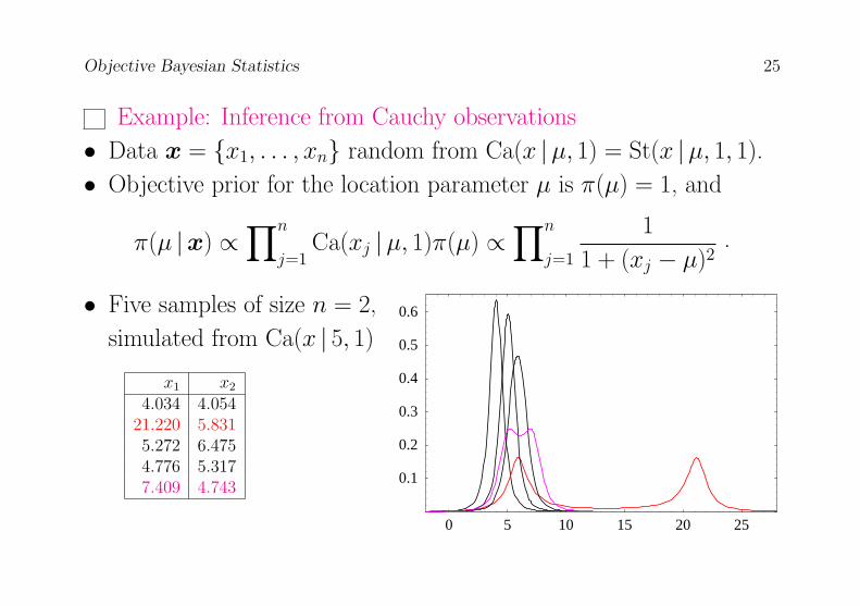
Example: Inference from Cauchy observations
• Data x = x1, . . . , xn random from Ca(x |µ, 1) = St(x |µ, 1, 1).
• Objective prior for the location parameter µ is π(µ) = 1, and
π(µ |x) ∝∏n
j=1Ca(xj |µ, 1)π(µ) ∝
∏n
j=1
1
1 + (xj − µ)2.
• Five samples of size n = 2,
simulated from Ca(x | 5, 1)
x1 x2
4.034 4.05421.220 5.8315.272 6.4754.776 5.3177.409 4.743
0 5 10 15 20 25
0.1
0.2
0.3
0.4
0.5
0.6
Objective Bayesian Statistics 26
Improper prior functions
• Objective Bayesian methods often use functions which play the role
of prior distributions but are not probability distributions. An im-
proper prior function is an non-negative function π(θ) such that∫Θ π(θ) dθ is not finite. The Cauchy example uses the improper prior
function π(µ) = 1, µ ∈ <.
• Let π(θ) be an improper prior function, Θi∞i=1 an increasing se-
quence approximating Θ, such that∫
Θiπ(θ) <∞, and let πi(θ)∞i=1
be the proper priors obtained by renormalizing π(θ) within the Θi’s.
Then, For any data x with likelihood p(x |θ), the sequence of poste-
riors πi(θ |x) converges intrinsically to π(θ |x) ∝ p(x |θ) π(θ).
• This procedure allows a systematic use of improper prior functions,
whenever this is required, as it is often the case in objective Bayesian
statistics.
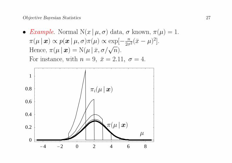
Objective Bayesian Statistics 27
• Example. Normal N(x |µ, σ) data, σ known, π(µ) = 1.
π(µ |x) ∝ p(x |µ, σ)π(µ) ∝ exp[− n2σ2(x− µ)2].
Hence, π(µ |x) = N(µ | x, σ/√n).
For instance, with n = 9, x = 2.11, σ = 4.
-4 -2 0 2 4 6 80
0.2
0.4
0.6
0.8
1
µπ(µ |x)
πi(µ |x)
Objective Bayesian Statistics 28
Sequential updating
• Prior and posterior are only terms relative to a particular set of
data.
• If data x = x1, . . . ,xn are sequentially presented, the final result
will be the same whether data are globally or sequentially processed.
π(θ |x1, . . . ,xi+1) ∝ p(xi+1 |θ) π(θ |x1, . . . ,xi).
The “posterior” at a given stage becomes the “prior” at the next.
• As one should certainly expect, Bayesian procedures with exchange-
able data are always independent of the particular order or grouping
in which the data are processed. This is often not the case with con-
ventional statistical procedures.
• Typically (but not always), the new posterior, π(θ |x1, . . . ,xi+1),
is more concentrated around the true value than π(θ |x1, . . . ,xi).
Objective Bayesian Statistics 29
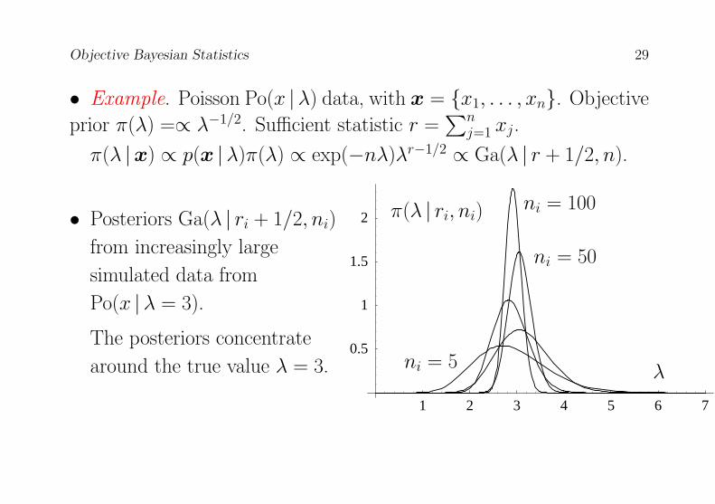
• Example. Poisson Po(x |λ) data, with x = x1, . . . , xn. Objective
prior π(λ) =∝ λ−1/2. Sufficient statistic r =∑n
j=1 xj.
π(λ |x) ∝ p(x |λ)π(λ) ∝ exp(−nλ)λr−1/2 ∝ Ga(λ | r + 1/2, n).
1 2 3 4 5 6 7
0.5
1
1.5
2
λ
π(λ | ri, ni) ni = 100
ni = 50
ni = 5
• Posteriors Ga(λ | ri + 1/2, ni)
from increasingly large
simulated data from
Po(x |λ = 3).
The posteriors concentrate
around the true value λ = 3.
Objective Bayesian Statistics 30
Nuisance parameters
• In general the vector of interest is not the whole parameter vector θ,
but some function φ = φ(θ) of possibly lower dimension.
• By Bayes’ theorem π(θ |x) ∝ p(x |θ) π(θ). Let ω = ω(θ) ∈ Ω
be another function of θ such that ψ = φ,ω is a bijection of θ,
and let J(ψ) = (∂θ/∂ψ) be the Jacobian of the inverse function ψ =
ψ(θ). From probability theory, π(ψ |x) = |J(ψ)|[π(θ |x)
]θ=θ(ψ)
and π(φ |x) =∫
Ω π(φ,ω |x) dω. Any valid conclusion on φ will be
contained in π(φ |x).
• Particular case: marginal posteriors. If model is expressed in terms
of vector of interest φ, and vector of nuisance parameters ω, so that
p(x |θ) = p(x |φ,ω), specify the prior π(θ) = π(φ) π(ω |φ); get the
joint posterior π(φ,ω |x) ∝ p(x |φ,ω) π(ω |φ) π(φ), and integrate
out ω, so that π(φ |x) ∝ π(φ)∫
Ω p(x |φ,ω) π(ω |φ) dω.
Objective Bayesian Statistics 31
Inferences about a Normal mean
• Data x = x1, . . . xn random from N(x |µ, σ) with likelihood
p(x |µ, σ) ∝ σ−n exp[−ns2 + (x− µ)2/(2σ2)],
where nx =∑
i xi, and ns2 =∑
i(xi − x)2.
• The objective prior is π(µ, σ) = σ−1, uniform in both µ and log(σ);
the corresponding joint posterior is
π(µ, σ |x) ∝ σ−(n+1) exp[−ns2 + (x− µ)2/(2σ2)].
• Hence, the marginal posterior for µ is
π(µ |x) ∝∫ ∞
0
π(µ, σ |x) dσ ∝ [s2 + (x− µ)2]−n/2
which is the kernel of the Student density
pi(µ |x) = St(µ | x, s/√n− 1, n− 1).
Objective Bayesian Statistics 32
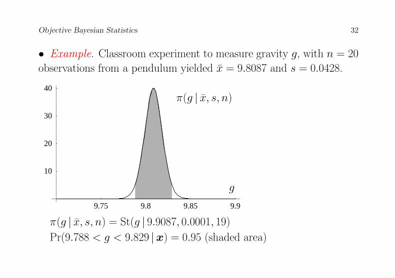
• Example. Classroom experiment to measure gravity g, with n = 20
observations from a pendulum yielded x = 9.8087 and s = 0.0428.
9.75 9.8 9.85 9.9
10
20
30
40π(g | x, s, n)
g
π(g | x, s, n) = St(g | 9.9087, 0.0001, 19)
Pr(9.788 < g < 9.829 |x) = 0.95 (shaded area)
Objective Bayesian Statistics 33
Restricted parameter space
• The range of θ values is often restricted by contextual considerations.
If θ is known to belong to Θc ⊂ Θ, so that π(θ) > 0 iff θ ∈ Θc, the
use of Bayes’ theorem yields
π(θ |x,θ ∈ Θc) =π(θ |x)∫
Ωcπ(θ |x) dθ
, if θ ∈ Θc,
and 0 otherwise.
• Thus, to incorporate a restriction, it suffices to renormalize the
unrestricted posterior distribution to the set Θc ⊂ Θ of admissible
parameter values.
• This is often very important in applications. Yet, incorporation of
parameter restrictions is often not possible in conventional, frequentist
statistics.
Objective Bayesian Statistics 34
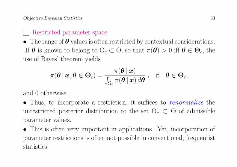
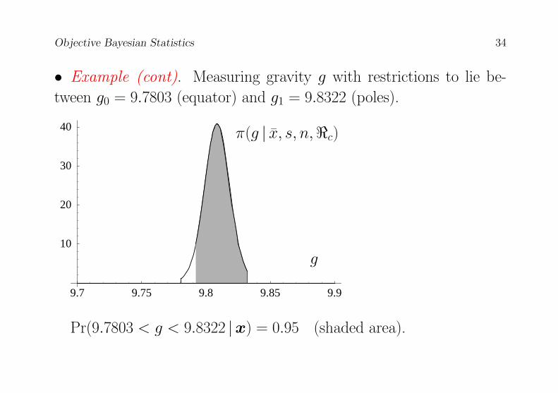
• Example (cont). Measuring gravity g with restrictions to lie be-
tween g0 = 9.7803 (equator) and g1 = 9.8322 (poles).
9.7 9.75 9.8 9.85 9.9
10
20
30
40
g
π(g | x, s, n,<c)
Pr(9.7803 < g < 9.8322 |x) = 0.95 (shaded area).
Objective Bayesian Statistics 35
Asymptotic behaviour, discrete case
• If the parameter space Θ = θ1, θ2, . . . is countable and the true
parameter value θt is distinguishable from all the others, so that
δp(x |θt), p(x |θi)) > 0, for all i 6= t,
then the posterior converges to a degenerate distribution with proba-
bility one on the true value:
limn→∞
π(θt |x1 . . . ,xn) = 1
limn→∞
π(θi |x1 . . . ,xn) = 0, i 6= t.
• To prove this, take logarithms is Bayes’ theorem, define
zi = log[p(x |θi)/p(x |θt)],
and use the strong law of large numbers on the n i.i.d. random variables
z1, . . . , zn.
Objective Bayesian Statistics 36
• For instance, in probabilistic diagnosis the posterior probability of
the true disease converges to one as new relevant information accumu-
lates, provided the model distinguishes the probabilistic behaviour of
data under the true disease from its behaviour under the other alter-
natives.
• If the true value of the parameter id not in Θ the posterior concen-
trates on the closest model in the intrinsic discrepancy sense, i.e., in
that value θ∗ such that
θ∗ = arg minθi∈Θ
δp(x |θt), p(x |θi).
Objective Bayesian Statistics 37
Asymptotic behaviour, continuous case
• If the parameter θ is one-dimensional and continuous, so that
Θ ⊂ <, and the model p(x | θ), x ∈ X is regular (basically, Xdoes not depend on θ, and p(x | θ) is twice θ differentiable)
• Then, as n→∞, π(θ |x1, . . . ,xn) converges intrinsically
to a normal distribution with mean at the mle estimator θ,
and with variance v(x1, . . . ,xn, θ), where
v−1(x1, . . . ,xn, θ) = −∑n
j=1∂2
∂θ2log[p(xj | θ]
• To prove this, write Bayes’ theorem as
π(θ |x1, . . . ,xn) ∝ exp[log π(θ) +∑n
j=1 log p(xj | θ)],
and expand∑n
j=1 log p(xj | θ)] about its maximum, the mle θ.
• The result is easily extended to the multivariate case θ = θ1, . . . , θk,to obtain a limiting k-variate normal centered at θ, and with a disper-
sion matrix V (x1, . . . ,xn, θ) which generalizes v(x1, . . . ,xn, θ).
Objective Bayesian Statistics 38
Asymptotic behaviour, continuous case. Simpler form
• Using the strong law of large numbers on the sums above a simpler,
less precise approximation is obtained:
• If the parameter θ = θ1, . . . , θk is continuous, so that Θ ⊂ <kand the model p(x | θ), x ∈ X is regular, so that X does not de-
pend on θ and p(x |θ) is twice differentiable with respect to each of
the θi’s, then, as n → ∞, π(θ |x1, . . . ,xn) converges intrinsically to
a multivariate normal distribution with mean the mle θ and preci-
sion matrix (inverse of the dispersion or variance-covariance matrix)
nF (θ), where F (θ) is Fisher’s matrix, of general element
Fij(θ) = −Ex |θ[∂2
∂θi∂θjlog p(x |θ)].
Objective Bayesian Statistics 39
• The properties of the multivariate normal easily yield from the last
result the asymptotic forms for the marginal and the conditional pos-
terior distributions of any subgroup of the θj’s.
• In one dimension,
π(θ |x1, . . . ,xn) ≈ N(θ | θ, [nF (θ)]−1/2)
a normal density centered at the mle θ with precision nF (θ), where
F (θ) is Fisher’s function,
F (θ) = −Ex | θ[∂2 log p(x | θ)/∂θ2].
Objective Bayesian Statistics 40
Example: Asymptotic approximation with Poisson data
• Data x = x1, . . . , xn a random sample from
Po(x |λ) ∝ e−λλx/x!
Hence, p(x |λ) ∝ e−nλλr, r = Σj xj, and λ = r/n.
• Fisher’s function is F (λ) = −Ex |λ
[∂2
∂λ2 log Po(x |λ)]
= 1λ
• The objective prior function is π(λ) = F (λ)1/2 = λ−1/2.
Hence π(λ |x) ∝ e−nλλr−1/2 which is the kernel of the Gamma
distribution
π(λ |x) = Ga(λ | r + 1/2, n).
• The Normal approximation is
π(λ |x) ≈ Nλ | λ, (nF (λ))−1/2 = Nλ | r/n,√r/n.
Objective Bayesian Statistics 41
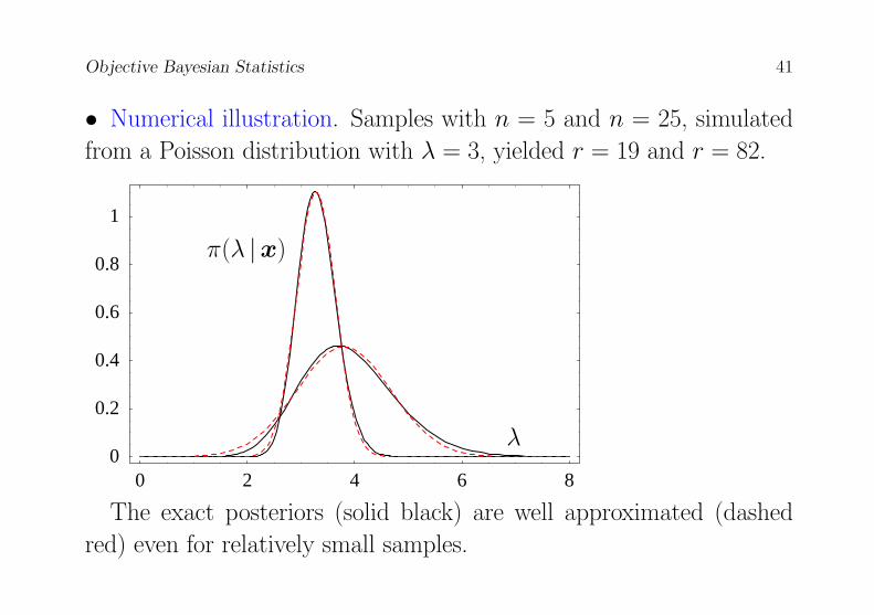
• Numerical illustration. Samples with n = 5 and n = 25, simulated
from a Poisson distribution with λ = 3, yielded r = 19 and r = 82.
0 2 4 6 80
0.2
0.4
0.6
0.8
1
λ
π(λ |x)
The exact posteriors (solid black) are well approximated (dashed
red) even for relatively small samples.
Objective Bayesian Statistics 42
Reference Analysis
No Relevant Initial Information
• Identify the mathematical form of a “noninformative” prior: One
with minimal effect, relative to the data, on the posterior distribu-
tion of the quantity of interest. Intuitive basis:
(i) Use information theory to measure the amount on information
about the quantity of interest to be expected from the data, which
depends on prior knowledge.
(ii) Define the missing information about the quantity of interest
as that which infinite independent replications of the experiment
could possible provide.
(iii) Define the reference prior as that which maximizes the missing
information about the quantity if interest.
Objective Bayesian Statistics 43
Expected information from the data
• Given model p(x | θ),x ∈ X , θ ∈ Θ, the amount of information
IθX , p(θ) which may be expected to be provided by x, about the
value of θ is defined by
IθX , p(θ) = δp(x, θ), p(x)p(θ),
the intrinsic discrepancy between the joint distribution p(x, θ) and
the product of their marginals p(x)p(θ), which is the instrinsic asso-
ciation between the random quantities x and θ.
• This is related to Shannon mutual information between x and θ,
Sp(x, θ) =∫X∫
Θ p(x, θ) log p(x,θ)p(x)p(θ) dx dθ, while δp(x, θ), p(x)p(θ)
is min[∫ ∫
p(x, θ) log p(x,θ)p(x)p(θ) dx dθ,
∫ ∫p(x)p(θ) log p(x)p(θ)
p(x,θ) dx dθ].
Often, but not always, the minimum is attained by integrating with
the joint density, in which case, IθX , π(θ) = Sp(x, θ).
Objective Bayesian Statistics 44
• Consider IθX k, p(θ) the information about θ which may be ex-
pected from k conditionally independent replications of the original
setup.
As k → ∞, this would provide any missing information about θ.
Hence, as k → ∞, the functional IθX k, π(θ) will approach the
missing information about θ associated with the prior p(θ).
• Let πk(θ) be the prior which maximizes IθX k, p(θ) in the class Pof strictly positive prior distributions compatible with accepted as-
sumptions on the value of θ (which could be the class of all strictly
positive priors).
The reference prior π∗(θ) is the limit as k → ∞ (in a sense to be
made precise) of the sequence of priors πk(θ), k = 1, 2, . . ..
Objective Bayesian Statistics 45
Reference priors in the finite case
• If θ may only take a finite number m of different values θ1, . . . , θmand p(θ) = p1, . . . , pm, with pi = Pr(θ = θi), then
limk→∞ IθX k, p(θ) = H(p1, . . . , pm) = −
∑mi=1 pi log(pi),
that is, the entropy of the prior distribution p1, . . . , pm.• In the finite case, with no additional structure,the reference prior is
that with maximum entropy within the class P of priors compatible
with accepted assumptions (cf. Statistical Physics).
• If, in particular, P contains all priors over θ1, . . . , θm, the refer-
ence prior is the uniform prior, π(θ) = 1/m, . . . , 1/m (cf. Bayes-
Laplace postulate of insufficient reason) .
• Example. Prior p1, p2, p3, p4 in genetics problem with p1 = 2p2.
Reference prior (maximum entropy given restriction) is
π(p) = 0.324, 0.162, 0.257, 0.257.
Objective Bayesian Statistics 46
Reference priors in one-dimensional continuous case
• Let πk(θ) be the prior which maximizes IθX k, π(θ) in the class Pof acceptable priors. For any datax ∈ X , let πk(θ |x) ∝ p(x | θ) πk(θ)
be the corresponding posterior.
• The reference posterior density π∗(θ |x) is defined to be the limit
of the sequence πk(θ |x), k = 1, 2, . . .. A reference prior function
π∗(θ) is any positive function such that, for all x ∈ X , π∗(θ |x) ∝p(x | θ) π∗(θ). This is defined up to an (irrelevant) arbitrary constant.
• Let x(k) ∈ X k be the result of k independent replications of x ∈ X .
The exact expression for πk(θ) (cf. calculus of variations) is
πk(θ) = exp [ Ex(k) | θlog πk(θ |x(k))] (a geometric average).
• This formula may be used, by repeated simulation from p(x | θ)
for different θ values, to obtain a numerical approximation to the
reference prior.
Objective Bayesian Statistics 47
Reference priors under regularity conditions
• Let θk = θ(x(k)) be a consistent, asymptotically sufficient estimator
of θ. In regular problems this is often the case with the mle θ.
• The exact expression for πk(θ) then becomes, for large k,
πk(θ) ≈ exp[Eθk | θlog πk(θ | θk)].As k →∞ this converges to πk(θ | θk)|θk=θ.
• Let θk = θ(x(k)) be a consistent, asymptotically sufficient estimator
of θ. Let π(θ | θk) be any asymptotic approximation to π(θ |x(k)), the
posterior distribution of θ. The reference prior may then be analyti-
cally computed as π∗(θ) = π(θ | θk)|θk=θ.
• Under regularity conditions, the posterior distribution of θ is asymp-
totically Normal, with mean θ and precision nF (θ), where
F (θ) = −Ex | θ[∂2 log p(x | θ)/∂θ2] is Fisher’s information function.
Hence, using the expression above, π∗(θ) = F (θ)1/2 (Jeffreys’ rule).
Objective Bayesian Statistics 48
One nuisance parameter
• Two parameters: reduce the problem to a sequential application
of the one parameter case. Model is p(x | θ, λ, θ ∈ Θ, λ ∈ Λ and a
θ-reference prior π∗θ(θ, λ) is required. Two steps:
(i) Conditional on θ, p(x | θ, λ) only depends on λ, and it is possible
to obtain the conditional reference prior π∗(λ | θ).
(ii) If π∗(λ | θ) is a proper distribution, integrate out λ to get the
one-parameter model p(x | θ) =∫
Λ p(x | θ, λ) π∗(λ | θ) dλ, and use the
one-parameter solution to obtain π∗(θ).
• The θ-reference prior is then π∗θ(θ, λ) = π∗(λ | θ) π∗(θ).
• The required reference posterior is π∗(θ |x) ∝ p(x | θ)π∗(θ).
Objective Bayesian Statistics 49
• If π∗(λ | θ) is an improper prior function, proceed within an increas-
ing sequence Λi over which π∗(λ | θ) is integrable and, for given data
x, obtain the corresponding sequence of reference posteriors π∗i (θ |x,defined over the Λi’s.• The required reference posterior π∗(θ |x) is their intrinsic limit.
π∗(θ |x) = limi→∞
π∗i (θ |x).
• A θ-reference prior is any positive function such that, for any data x,
π∗(θ |x) ∝∫
Λ
p(x | θ, λ) π∗θ(θ, λ) dλ.

Objective Bayesian Statistics 50
The regular two-parameter continuous case
• Model p(x | θ, λ). If the joint posterior of (θ, λ) is asymptotically
normal, the θ-reference prior may be derived in terms of the corre-
sponding Fisher’s information matrix,
F (θ, λ) =
(Fθθ(θ, λ) Fθλ(θ, λ)
Fθλ(θ, λ) Fλλ(θ, λ)
), S(θ, λ) = F−1(θ, λ)
• The θ-reference prior is
π∗θ(θ, λ) = π∗(λ | θ) π∗(θ),
π∗(λ | θ) ∝ F1/2λλ (θ, λ), λ ∈ Λ,
and, if π∗(λ | θ) is proper,
π∗(θ) ∝ exp ∫
Λ
π∗(λ | θ) log[S−1/2θθ (θ, λ)] dλ, θ ∈ Θ.
Objective Bayesian Statistics 51
• If π∗(λ | θ) is not proper, integrations are to be performed within an
approximating sequence Λi to obtain a sequence π∗i (λ | θ) π∗i (θ),and the θ-reference prior π∗θ(θ, λ) is defined as its intrinsic limit,
π∗θ(θ, λ) = limi→∞
π∗i (λ | θ) π∗i (θ).
• Even if π∗(λ | θ) is improper, if
(i) θ and λ are variation independent, and
(ii) the functions Sθθ and Fλλ factorize such that
S−1/2θθ (θ, λ) ∝ fθ(θ) gθ(λ),
F1/2λλ (θ, λ) ∝ fλ(θ) gλ(λ),
Then the joint reference prior when θ is the quantity of interest is
π∗θ(θ, λ) = fθ(θ) gλ(λ).
Objective Bayesian Statistics 52
Example: Inference on normal parameters
• The information matrix for the normal model N(x |µ, σ) is
F (µ, σ) =
(σ−2 0
0 2σ−2
), S(µ, σ) =
(σ2 0
0 σ2/2
)Since µ and σ are variation independent, and both Fσσ and Sµµ fac-
torize, π∗(σ |µ) ∝ F1/2σσ ∝ σ−1, π∗(µ) ∝ S
−1/2µµ ∝ 1.
• The µ-reference prior is π∗µ(µ, σ) = π∗(σ |µ) π∗(µ) = σ−1, i.e.,
uniform on both µ and log σ.
• Since F (µ, σ) is diagonal the σ-reference prior is
π∗σ(µ, σ) = π∗(µ |σ)π∗(σ) = σ−1, the same as π∗µ(µ, σ).
• In fact, it may be shown that for all location-scale models, so that
p(x |µ, σ) = 1σf (x−µσ ), the reference priors for the location and scale
parameters are π∗µ(µ, σ) = π∗σ(µ, σ) = σ−1.
Objective Bayesian Statistics 53
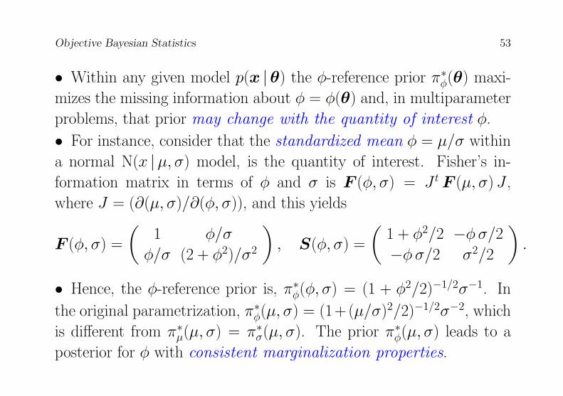
• Within any given model p(x |θ) the φ-reference prior π∗φ(θ) maxi-
mizes the missing information about φ = φ(θ) and, in multiparameter
problems, that prior may change with the quantity of interest φ.
• For instance, consider that the standardized mean φ = µ/σ within
a normal N(x |µ, σ) model, is the quantity of interest. Fisher’s in-
formation matrix in terms of φ and σ is F (φ, σ) = J tF (µ, σ) J ,
where J = (∂(µ, σ)/∂(φ, σ)), and this yields
F (φ, σ) =
(1 φ/σ
φ/σ (2 + φ2)/σ2
), S(φ, σ) =
(1 + φ2/2 −φσ/2
−φσ/2 σ2/2
).
• Hence, the φ-reference prior is, π∗φ(φ, σ) = (1 + φ2/2)−1/2σ−1. In
the original parametrization, π∗φ(µ, σ) = (1+ (µ/σ)2/2)−1/2σ−2, which
is different from π∗µ(µ, σ) = π∗σ(µ, σ). The prior π∗φ(µ, σ) leads to a
posterior for φ with consistent marginalization properties.
Objective Bayesian Statistics 54
Many parameters
• The reference algorithm generalizes to any number of parameters. If
the model is p(x |θ) = p(x | θ1, . . . , θm), a joint reference prior
π∗(φm |φm−1, . . . , φ1) × . . . × π∗(φ2 |φ1) × π∗(φ1) may sequentially
be obtained for each ordered parametrization, φ1(θ), . . . , φm(θ).Reference priors are invariant under reparametrization of the φi(θ)’s.
• The choice of the ordered parametrization φ1, . . . , φm describes
the particular prior required, namely that which sequentially
maximizes the missing information about each of the φi’s,
conditional on φ1, . . . , φi−1, for i = m,m− 1, . . . , 1.
• In many problems, the results are equal or similar for many param-
eterizations, but this is not necessarily the case. As a consequence, an
approximate overall reference prior is often pragmatically required.
Objective Bayesian Statistics 55
• An overall reference prior, one leading to marginal posteriors which
are not far from the appropriate reference posteriors for all quantities of
interest, may be obtained by minimizing the average intrinsic discrep-
ancy between the marginal and the reference posteriors. For details
sees Berger, Bernardo and Sun (2014).
• Example: Stein’s paradox. Data random from a m-variate normal
Nm(x |µ, I). The reference prior for any permutation of the µi’s is
uniform, and leads to appropriate posterior distributions for any of the
µi’s, but cannot be used if the quantity of interest is θ =∑
i µ2i , the
distance of µ to the origin, for this leads to an inconsistent estimation
of θ.
However, the reference prior for θ, πθ(µ) produces, an appropriate,
consistent marginal reference posterior for θ.
Objective Bayesian Statistics 56
Inference Summaries
Summarizing the posterior distribution
• The Bayesian final outcome of a problem of inference about any
unknown quantity θ is precisely the posterior density π(θ |x, C).
• Bayesian inference may be described as the problem of stating a
probability distribution for the quantity of interest encapsulating all
available information about its value.
• In one or two dimensions, a graph of the posterior probability den-
sity of the quantity of interest conveys an intuitive summary of the
main conclusions. This is greatly appreciated by users, and is an im-
portant asset of Bayesian methods.
• But graphical methods are not easily extended to more than two
dimensions and elementary quantitative conclusions are often required.
Objective Bayesian Statistics 57
The simplest forms to summarize the information contained in the
posterior distribution are closely related to the conventional concepts
of point estimation and interval estimation.
Point Estimation: Posterior mean and posterior mode
• It is often required to provide point estimates of relevant quanti-
ties. Bayesian point estimation is best described as a decision problem
where one has to choose a particular value θ as an approximate proxy
for the actual, unknown value of θ.
• Intuitively, any location measure of the posterior density π(θ |x)
may be used as a point estimator. When they exist, either
E[θ |x] =∫
Θ θ π(θ |x) dθ (posterior mean), or
Mo[θ |x] = arg supθ∈Θ π(θ |x) (posterior mode)
are often regarded as natural choices.
Objective Bayesian Statistics 58
• Lack of invariance. Neither the posterior mean not the posterior
mode are invariant under reparametrization. The point estimator ψ
of a bijection ψ = ψ(θ) of θ will generally not be equal to ψ(θ).
• In pure “inferential” applications, where one is requested to provide
a point estimate of the vector of interest without an specific application
in mind, it is difficult to justify a non-invariant solution:
The best estimate of, say, φ = log(θ) should be φ∗ = log(θ∗), but
this is not the case if the posterior mean or the posterior mode are used
as point estimators.
• Notice that most estimation procures in conventional statistics also
suffer from this lack of (intuitively necessary) invariance under repa-
rameterization. However, general invariant multivariate definitions of
point estimators is possible using Bayesian decision theory.
Objective Bayesian Statistics 59
Point Estimation: Posterior median
• In one-dimensional continuous problems the posterior median,
is easily defined and computed as
Me[θ |x] = q ;∫θ≤q π(θ |x) dθ = 1/2.
The one-dimensional posterior median has attractive properties:
(i) it is invariant under bijections, Me[φ(θ) |x] = φ(Me[θ |x]).
(ii) it exists and it is unique under very wide conditions.
(iii) it is rather robust under moderate perturbations of the data.
• The posterior median is often considered to be the best ‘automatic’
Bayesian point estimator in one-parameter continuous problems, but
its definition is not easily extended to a multiparameter setting.
Objective Bayesian Statistics 60
General Credible Regions
• To describe π(θ |x) it is often convenient to quote regions Θp ⊂ Θ
of given probability content p under π(θ |x). This is the intuitive basis
of graphical representations like boxplots.
• A subset Θp of the parameter space Θ such that∫Θpπ(θ |x) dθ = p and, hence, Pr(θ ∈ Θp |x) = p,
is a posterior p-credible region for θ.
• A credible region is invariant under reparametrization:
If Θp is p-credible for θ, φ(Θp) is a p-credible for φ = φ(θ).
• For any given p there are generally infinitely many credible regions
• Credible regions may be selected to have minimum size (length, area,
volume), resulting in highest probability density (HPD) regions, where
all points in the region have larger probability density than all points
outside.
Objective Bayesian Statistics 61
• Like their related modal estimates, HPD regions are not invariant.
Thus, the image φ(Θp) of an HPD region Θp will be a credible region
for φ, but will not generally be HPD.
There is no reason to restrict attention to HPD credible regions.
Credible Intervals
• In one-dimensional continuous problems, posterior quantiles are
often used to derive credible intervals.
• If θq = Qq[θ |x] is the q-quantile of the posterior distribution of θ,
the interval Θp = θ; θ ≤ θp is a p-credible region,
and it is invariant under reparameterization.
• Equal-tailed p-credible intervals of the form
Θp = θ; θ(1−p)/2 ≤ θ ≤ θ(1+p)/2are typically unique, and they invariant under reparametrization.
Objective Bayesian Statistics 62
• Example: Credible intervals for the normal mean.
• With model N(x |µ, σ), the reference posterior for µ given
x = x1, . . . , xn is π(µ |x) = St(µ | x, s/√n− 1, n− 1).
Hence the reference posterior distribution of
τ =√n− 1(µ− x)/s,
as a function of µ, is π(τ | x, s, n) = St(τ | 0, 1, n− 1).
• It then follows that the equal-tailed p-credible intervals for µ are
µ; µ ∈ x ± q(1−p)/2n−1 s/
√n− 1,
where q(1−p)/2n−1 is the (1− p)/2 quantile of a standard Student density
with n− 1 degrees of freedom.
• To study the long term behavior of these credible intervals, the ex-
pression√n− 1(µ − x)/s may also be analyzed, for fixed µ, as a
function of the data.
Objective Bayesian Statistics 63
Calibration
The fact that the sampling distribution of the statistic
t = t(x, s |µ, n) =√n− 1(µ− x)/s
is also an standard Student p(t |µ, n) = St(t | 0, 1, n−1) with the same
degrees of freedom implies that, in this example, objective Bayesian
credible intervals are also be exact frequentist confidence intervals.
• Exact numerical agreement (exact matching) between Bayesian
credible intervals and frequentist confidence intervals is however the
exception, not the norm.
• For large samples, convergence to normality implies approximate
numerical agreement. This provides a frequentist calibration to
objective Bayesian methods.
Objective Bayesian Statistics 64
• Exact numerical agreement is obviously impossible when the data
are discrete: Precise (non randomized) frequentist confidence intervals
do not exist in that case for most confidence levels.
The computation of Bayesian credible regions for continuous param-
eters is however precisely the same whether the data are discrete or
continuous.
• The coverage properties of credible regions obtained form different
objective priors is often computed to compare the behavior of the priors
used to derive them. Although exact numerical agreement of posterior
probabilities and average coverage is not to be expected, they should
be close to order O(n−1/2).
Objective Bayesian Statistics 65
Prediction
Posterior predictive distributions
• Data x = x1, . . . , xn, xi ∈ X , set of “homogeneous” observations.
Desired to predict the value of a future observation x ∈ X generated
by the same mechanism.
• From the foundations arguments the solution must be a probability
distribution p(x |x, K) describing the uncertainty on the value that x
will take, given data x and any other available knowledge K. This is
called the (posterior) predictive density of x.
• To derive p(x |x, K) it is necessary to specify the precise sense in
which the xi’s are judged to be homogeneous.
• It is often directly assumed that the data x = x1, . . . , xn consist
of a random sample from some statistical model.
Objective Bayesian Statistics 66
Posterior predictive distributions from random samples
• Let x = x1, . . . , xn, xi ∈ X , a random sample of size n from
the statistical model p(x |θ), x ∈ X ,θ ∈ Θ and let π(θ) a prior
distribution describing available knowledge (in any) about the value of
the parameter vector θ.
• The posterior predictive distribution is
p(x |x) = p(x |x1, . . . , xn) =
∫Θ
p(x |θ) π(θ |x) dθ.
This encapsulates all available information about the outcome of any
future observation x ∈ X from the same model.
• To prove this, make use the total probability theorem, to have
p(x |x) =∫
Θ p(x |θ,x) π(θ |x) dθ, and notice the new observation
x has been assumed to be conditionally independent of the observed
data x, so that p(x |θ,x) = p(x |θ).
Objective Bayesian Statistics 67
• The observable values x ∈ X may be either discrete or continuous
random quantities. In the discrete case, the predictive distribution will
be described by its probability mass function; in the continuous case,
by its probability density function. Both are denoted p(x |x).
Prediction in a Poisson process
• Data x = r1, . . . , rn random from Po(r |λ). The reference poste-
rior density of λ is π∗(λ |x) = Ga(λ | t + 1/2, n), where t = Σj rj.
The (reference) posterior predictive distribution is
p(r |x) = Pr[r | t, n] =
∫ ∞0
Po(r |λ) Ga(λ | t + 1/2, n) dλ
=nt+1/2
Γ(t + 1/2)
1
r!
Γ(r + t + 1/2)
(1 + n)r+t+1/2,
an example of a Poisson-Gamma probability mass function.
Objective Bayesian Statistics 68
• Example. Flash floods. No flash floods have been recorded on a
particular location in 10 consecutive years. Local authorities are inter-
ested in forecasting possible future flash floods. Using a Poisson model,
and assuming that meteorological conditions remain similar, the prob-
abilities that r flash floods will occur next year in that location are
given by the Poisson-Gamma mass function above, with t = 0 and
n = 10. This yields,
Pr[0 | t, n] = 0.953, Pr[1 | t, n] = 0.043, Pr[2 | t, n] = 0.003, . . ..
Prediction of Normal measurements
• Data x = x1, . . . , xn random from N(x |µ, σ). Reference prior
π∗(µ, σ) = σ−1 or, in terms of the precision λ = σ−2, π∗(µ, λ) = λ−1.
• The joint reference posterior, π∗(µ, λ |x) ∝ p(x |µ, λ) π∗(µ, λ), is
π∗(µ, λ |x) = N(µ | x, (nλ)−1/2) Ga(λ | (n− 1)/2, ns2/2).
Objective Bayesian Statistics 69
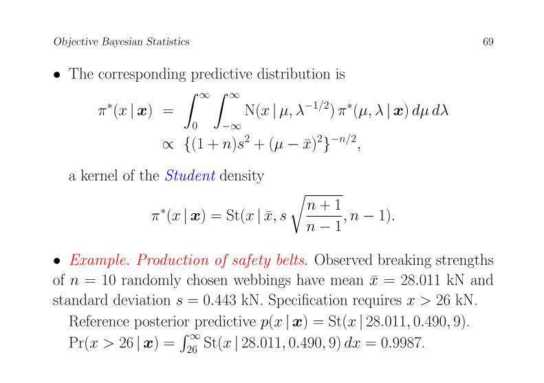
• The corresponding predictive distribution is
π∗(x |x) =
∫ ∞0
∫ ∞−∞
N(x |µ, λ−1/2) π∗(µ, λ |x) dµ dλ
∝ (1 + n)s2 + (µ− x)2−n/2,
a kernel of the Student density
π∗(x |x) = St(x | x, s√n + 1
n− 1, n− 1).
• Example. Production of safety belts. Observed breaking strengths
of n = 10 randomly chosen webbings have mean x = 28.011 kN and
standard deviation s = 0.443 kN. Specification requires x > 26 kN.
Reference posterior predictive p(x |x) = St(x | 28.011, 0.490, 9).
Pr(x > 26 |x) =∫∞
26 St(x | 28.011, 0.490, 9) dx = 0.9987.
Objective Bayesian Statistics 70
Regression
• In prediction problems there is often additional information from
relevant covariates. The data structure consists of set of pairs (yi,vi),where both the observables yi and the covariates vi may be vectors of
any dimension. Given a new observation, with v known, one wants to
predict the corresponding value of y. Formally, one has to compute
the predictive distribution py |v, (y1,v1), . . . (yn,vn).• A model p(y |v,θ),y ∈ Y ,θ ∈ Θ is needed which makes precise
the probabilistic relationship between y and v. The simplest option
assumes a linear dependency of the form
p(y |v,θ) = N(y |V β,Σ),
but far more complex structures are common in applications.
Objective Bayesian Statistics 71
• Univariate linear regression on k covariates.
Y ⊂ <, v = v1, . . . , vk.p(y |v,β, σ) = N(y |vβ, σ2), β = β1, . . . , βkt.Data is x = y,V , where y = y1, . . . , ynt,and V the n× k matrix with the vi’s as rows.
The likelihood is p(y |V ,β, σ) = Nn(y |V β, σ2In),
and the reference prior is π∗(β, σ) = σ−1.
• The predictive posterior is the Student density
p(y |v,y,V ) = St(y |vβ, f (v,V )ns2
n− k, n− k)
β = (V tV )−1V ty, ns2 = (y − vβ)t(y − vβ) and
f (v,V ) = 1 + v(V tV )−1vt.
Objective Bayesian Statistics 72
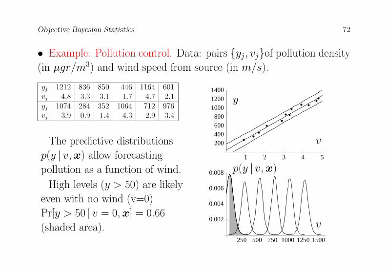
• Example. Pollution control. Data: pairs yj, vjof pollution density
(in µgr/m3) and wind speed from source (in m/s).
yj 1212 836 850 446 1164 601vj 4.8 3.3 3.1 1.7 4.7 2.1yj 1074 284 352 1064 712 976vj 3.9 0.9 1.4 4.3 2.9 3.4
250 500 750 1000 1250 1500
0.002
0.004
0.006
0.008
1 2 3 4 5
200400600800
100012001400
v
y
v
p(y | v,x)
The predictive distributions
p(y | v,x) allow forecasting
pollution as a function of wind.
High levels (y > 50) are likely
even with no wind (v=0)
Pr[y > 50 | v = 0,x] = 0.66
(shaded area).
Objective Bayesian Statistics 73
Hierarchical Models
Exchangeability
• Random quantities are often “homogeneous” in the precise sense that
only their values matter, not the order in which they appear. The set of
random vectors x1, . . . ,xn is exchangeable iff their joint distribution
is invariant under permutations. An infinite sequence xj of random
vectors is exchangeable if all its finite subsequences are exchangeable.
• Any random sample is exchangeable. The representation theorem
establishes that if observations x1, . . . ,xn are exchangeable, they
are a a random sample from some model p(x |θ),θ ∈ θ, labeled
by a parameter vector θ, defined as the limit (as n → ∞) of some
function of the xi’s. Information about θ in prevailing conditions C is
necessarily described by some probability distribution π(θ |C).
Objective Bayesian Statistics 74
• Formally, the joint density of any finite set of exchangeable observa-
tions x1, . . . ,xn has an integral representation of the form
p(x1, . . . ,xn |C) =∫θ
∏ni=1 p(xi |θ) π(θ |C) dθ.
• Complex data structures may often be usefully described by partial
exchangeability assumptions.
• Example: Public opinion. Sample k different regions in the coun-
try. Sample ni citizens in region i, and record whether or not (yij = 1
or yij = 0) citizen j would vote A. Assuming exchangeable citizens
within each region implies
p(yi1, . . . , yini |θ) =∏ni
j=1p(yij | θi) = θrii (1− θi)ni−ri,
where θi is the (unknown) proportion of citizens in region i voting A
and ri = Σjyij is the number of citizens voting A in region i.
Objective Bayesian Statistics 75
Assuming regions exchangeable within the country similarly yields
p(θ1, . . . , θkgφ) =∏k
i=1π(θi |φ)
for some probability distribution π(θ |φ) describing the political vari-
ation within the regions.
Often a general Beta density π(θ |φ) = Be(θ |α, β) is chosen to
describe this variation.
• The resulting two-stages hierarchical Binomial-Beta model
x = y1, . . . ,yk, yi = yi1, . . . , yini, random from Bi(y | θi),θ1, . . . , θk, random from Be(θ |α, β)
provides a far richer model than (the rather unrealistic, but too
frequently used) simple binomial model.
Objective Bayesian Statistics 76
• Example: Biological response. Sample k different animals of the
same species in a specific environment. Control ni times animal i and
record his responses yi1, . . . ,yini to prevailing conditions. Assuming
exchangeable observations within each animal implies
p(yi1, . . . ,yini |θ) =∏ni
j=1p(yij |θi).
Often a normal model p(yij |θi) = Nr(y |µi,Σ1) is chosen, where
the dimension r is the number of biological responses measured.
Assuming exchangeable animals within the environment leads to
p(µ1, . . . ,µkgφ) =∏k
i=1π(µi |φ)
for some probability distribution π(µ |φ) describing the biological vari-
ation within the species.
Often a normal model π(µ |φ) = Nr(µ |µ0,Σ2) is chosen.
Objective Bayesian Statistics 77
• The two-stages hierarchical multivariate Normal-Normal model
x = y1, . . . ,yk, yi = yi1, . . . ,yini, random from Nr(y |µi,Σ1),
µ1, . . . ,µk, random from Nr(µ |µ0,Σ2)
provides a far richer model than (again unrealistic) simple multivariate
normal sampling.
• Finer subdivisions, such as subspecies within each species, similarly
lead to hierarchical models with more stages.
Bayesian analysis of hierarchical models
• A two-stages hierarchical model has the general form
x = y1, . . . ,yk, yi = zi1, . . . ,ziniyi random sample of size ni from p(z |θi), θi ∈ Θ,
θ1, . . . ,θk, random of size k from π(θ |φ), φ ∈ Φ.
Objective Bayesian Statistics 78
• To analyze a hierarchical model
(i) Specify a prior distribution (or a reference prior function)
π(φ) for the hyperparameter vector φ.
(ii) Use standard probability theory to compute all desired
posterior distributions:
π(φ |x) for inferences about the hyperparameters,
π(θi |x) for inferences about the parameters,
π(ψ |x) for inferences about the any function ψ = ψ(θ1, . . . ,θk),
π(y |x) for predictions on future observations,
π(t |x) for predictions on any function t = t(y1, . . . ,ym)
• Markov Chain Monte Carlo (MCMC) based software available for
the necessary computations.
Objective Bayesian Statistics 79
Integrated Reference Analysis• The basic machinery of Baysian inference has been reviewed above.
However, there is no obvious agreement on the appropriate Bayesian
solution to even simple (textbook) stylized problems:
Best point estimate for the normal variance?
Inferences on the correlation coefficient of a bivariate normal?
Comparing two normal means or two binomial proportions?
Testing compatibility of the normal mean with a precise value?
• Let alone in problems within complex models with many parameters!
Proposal: Return to basics and use decision-theoretic machinery.
Objective Bayesian Statistics 80
Structure of a Decision Problem
Alternatives, consequences, relevant events
• A decision problem if two or more possible courses of action; A is
the class of possible actions.
• For each a ∈ A, Θa is the set of relevant events, those may affect
the result of choosing a.
• Each pair a,θ, θ ∈ Θa, produces a consequence c(a,θ) ∈ Ca. In
this context, θ if often referred to as the parameter of interest.
• The class of pairs (Θa, Ca), a ∈ A describes the structure of the
decision problem. Without loss of generality, it may be assumed that
the possible actions are mutually exclusive, for otherwise the appropri-
ate Cartesian product may be used.
Objective Bayesian Statistics 81
• In many problems the class of relevant events Θa is the same for all
a ∈ A. Even if this is not the case, a comprehensive parameter space
Θ may be defined as the union of all the Θa.
Foundations of decision theory
• Different sets of principles capture a minimum collection of logical
rules required for “rational” decision-making. These are axioms with
strong intuitive appeal.
• Their basic qualitative structure consists of:
(i) The transitivity of preferences:
If a1 > a2 given C, and a2 > a3 given C, then a1 > a3 given C.
(ii) The sure-thing principle:
If a1 > a2 given C and E, and a1 > a2 given C and not E
then a1 > a2 given C.
Objective Bayesian Statistics 82
• To make possible quantitative statements, this is supplemented by
(iii) The existence of standard events
These are events of known plausibility, which may be used as a unit
of measurement, and have the properties of a probability measure.
• These axioms are not a description of human decision-making,
but a normative set of principles defining coherent decision-making.
• There are many different axiom sets published with different levels
of generality, but they all basically lead to the same set of conclusions,
namely:
Objective Bayesian Statistics 83
• The consequences of making mistakes should be evaluated in terms
of a real-valued loss function `(a,θ) which specifies, on a numerical
scale, their degree of undesirability.
• The uncertainty about the parameter of interest θ should be mea-
sured with a probability distribution p(θ |C)
p(θ |C) ≥ 0, θ ∈ Θ,
∫Θ
p(θ |C) dθ = 1,
describing all available knowledge about its value, given the condi-
tions C under which the decision must be taken.
• The relative undesirability of available actions a ∈ A is measured
by their expected loss
`[a |C] =
∫Θ
`(a,θ) p(θ |C) dθ, a ∈ A.
• The best action is that with the smallest expected loss.
Objective Bayesian Statistics 84
Decision structure of Inference Summaries
• Assume data z have been generated as one random observation form
Mz = p(z |θ,λ), z ∈ Z,θ ∈ Θ,λ ∈ Λ, where θ is the vec-
tor of interest and λ a nuisance parameter vector, and let p(θ,λ) =
p(λ |θ) p(θ) be the assumed joint prior.
• Given data z and assuming model Mz, the complete solution to
all inference questions about θ is contained in the marginal posterior
p(θ | z), derived by standard use of probability theory.
• As mentioned before, appreciation of p(θ | z) may be enhanced by
providing both point and region estimates of the vector of interest θ,
and by declaring whether or not some context-suggested specific value θ0
(or maybe a set of values Θ0), is (are) compatible with the observed
data z. This provides useful (and often required) summaries of p(θ | z).
Objective Bayesian Statistics 85
• All these summaries may be framed as different decision problems
which use precisely the same loss function `θ0, (θ,λ) describing, as
a function of the (unknown) (θ,λ) values which have generated the
data, the loss to be suffered if, working with model Mz, the value θ0
were used as a proxy for the unknown value of θ.
• The results dramatically depend on the choices made for both the
prior and the loss functions but, given z, only depend on those through
the expected loss, `(θ0 | z) =∫
Θ
∫Λ `θ0, (θ,λ) p(θ,λ | z) dθdλ.
• As a function of θ0 ∈ Θ, `(θ0 | z) is a measure of the unacceptability
of all possible values of the vector of interest. This provides a dual,
complementary information on all θ values (on a loss scale) to that
provided by the posterior p(θ | z) (on a probability scale).
Objective Bayesian Statistics 86
Point estimation
To choose a point estimate for θ is a decision problem where the
action space is the class Θ of all possible θ values.
Definition 1 The Bayes estimator θ∗(z) = arg infθ0∈Θ `(θ0 | z) is
that which minimizes the posterior expected loss.
• Conventional examples include the ubiquitous quadratic loss
`θ0, (θ,λ) = (θ0 − θ)t(θ0 − θ), which yields the posterior mean as
the Bayes estimator, and the zero-one loss on a neighborhood of the
true value, which yields the posterior mode a a limiting result.
• Bayes estimators with conventional loss functions are typically not
invariant under one to one transformations. Thus, the Bayes estimator
under quadratic loss of a variance s not the square of the Bayes estima-
tor of the standard deviation. This is rather difficult to explain when
one merely wishes to report an estimate of some quantity of interest.
Objective Bayesian Statistics 87
Region estimation
Bayesian region estimation is achieved by quoting posterior credible
regions. To choose a q-credible region is a decision problem where the
action space is the class of subsets of Θ with posterior probability q.
Definition 2 (Bernardo, 2005). A Bayes q-credible region Θ∗q(z) is
a q-credible region where any value within the region has a smaller
posterior expected loss than any value outside the region, so that
∀θi ∈ Θ∗q(z), ∀θj /∈ Θ∗q(z), `(θi | z) ≤ `(θj | z).
• The quadratic loss yields credible regions with those θ values closest,
in the Euclidean sense, to the posterior mean. A zero-one loss function
leads to highest posterior density (HPD) credible regions.
• Conventional Bayes regions are often not invariant: HPD regions in
one parameterization will not transform to HPD regions in another.
Objective Bayesian Statistics 88
Precise hypothesis testing
• Consider a value θ0 which deserves special consideration. Testing
the hypothesis H0 ≡ θ = θ0 is as a decision problem where the
action space A = a0, a1 contains only two elements: to accept (a0)
or to reject (a1) the hypothesis H0.
• Foundations require to specify the loss functions `ha0, (θ,λ) and
`ha1, (θ,λ) measuring the consequences of accepting or rejecting H0
as a function of (θ,λ). The optimal action is to reject H0 iif∫Θ
∫Λ[`ha0, (θ,λ) − `ha1, (θ,λ)] p(θ,λ | z) dθdλ > 0.
• Hence, only ∆`hθ0, (θ,λ) = `ha0, (θ,λ)−`ha1, (θ,λ), which
measures the conditional advantage of rejecting, must be specified.
Objective Bayesian Statistics 89
• Without loss of generality, the function ∆`h may be written as
∆`hθ0, (θ,λ) = `θ0, (θ,λ) − `0
where (precisely as in estimation), `θ0, (θ,λ) describes, as a function
of (θ,λ), the non-negative loss to be suffered if θ0 were used as a proxy
for θ, and the constant `0 > 0 describes (in the same loss units) the
context-dependent non-negative advantage of accepting θ = θ0 when
it is true.
Definition 3 (Bernardo and Rueda, 2002). The Bayes test criterion
to decide on the compatibility of θ = θ0 with available data z is to
reject H0 ≡ θ = θ0 if (and only if), `(θ0 | z) > `0, where `0 is a
context dependent positive constant.
• The compound case may be analyzed by separately considering each
of the values which make part of the compound hypothesis to test.
Objective Bayesian Statistics 90
• Using a zero-one loss function, so that the loss advantage of reject-
ing θ0 is equal to one whenever θ 6= θ0 and zero otherwise, leads
to rejecting H0 if (and only if) Pr(θ = θ0 | z) < p0 for some context-
dependent p0. Use of this loss requires the prior probability Pr(θ = θ0)
to be strictly positive. If θ is a continuous parameter this forces the
use of a non-regular “sharp” prior, concentrating a positive probability
mass at θ0, the solution early advocated by Jeffreys.
This formulation (i) implies the use of radically different priors for
hypothesis testing than those used for estimation, (ii) precludes the use
of conventional, often improper, ‘noninformative” priors, and (iii) may
lead to the difficulties associated to Jeffreys-Lindley paradox.
• The quadratic loss function leads to rejecting a θ0 value whenever
its Euclidean distance to E[θ | z], the posterior expectation of θ, is
sufficiently large.
Objective Bayesian Statistics 91
• The use of continuous loss functions (such as the quadratic loss)
permits the use in hypothesis testing of precisely the same priors that
are used in estimation.
• With conventional losses the Bayes test criterion is not invariant
under one-to-one transformations. Thus, if φ(θ) is a one-to-one trans-
formation of θ, rejecting θ = θ0 does not generally imply rejecting
φ(θ) = φ(θ0).
• The threshold constant `0, which controls whether or not an expected
loss is too large, is part of the specification of the decision problem,
and should be context-dependent. However a judicious choice of the
loss function leads to calibrated expected losses, where the relevant
threshold constant has an immediate, operational interpretation.
Objective Bayesian Statistics 92
Loss Functions in Inference Problems• A dissimilarity measure δpz, qz between two probability densities
pz and qz for a random vector z ∈ Z should be
(i) non-negative, and zero if (and only if) pz = qz a.e.,
(ii) invariant under one-to-one transformations of z,
(iii) symmetric, so that δpz, qz = δqz, pz,(iv) defined for densities with strictly nested supports.
Definition 4 The intrinsic discrepancy δp1, p2 is
δp1, p2 = min [κp1 | p2, κp2 | p1 ]
where κpj | pi =∫
Zipi(z) log[pi(z)/pj(z)] dz is the (KL) diver-
gence of pj from pi. The intrinsic discrepancy between p and a
family F = qi, i ∈ I is the intrinsic discrepancy between p and
the closest of them, δp,F = infq,∈F δp, q.
Objective Bayesian Statistics 93
The intrinsic discrepancy loss function
Definition 5 ConsiderMz = p(z |θ,λ), z ∈ Z,θ ∈ Θ,λ ∈ Λ.The intrinsic discrepancy loss from using θ0 as a proxy for θ is
the intrinsic discrepancy between the true model and the class of
models with θ = θ0, M0 = p(z |θ0,λ0), z ∈ Z,λ0 ∈ Λ,
`δθ0, (θ,λ) |Mz = infλ0∈Λ
δpz(· |θ,λ), pz(· |θ0,λ0).
Invariance
• For any one-to-one reparameterization φ = φ(θ) and ψ = ψ(θ,λ),
`δθ0, (θ,λ) |Mz = `δφ0, (φ,ψ) |Mz.This yields invariant Bayes point and region estimators, and invariant
Bayes hypothesis testing procedures.
Objective Bayesian Statistics 94
Reduction to sufficient statistics
• If t = t(z) is a sufficient statistic for modelMz, one may also work
with marginal modelMt = p(t |θ,λ), t ∈ T ,θ ∈ Θ,λ ∈ Λ since
`δθ0, (θ,λ) |Mz = `δθ0, (θ,λ) |Mt.
Additivity
• If data consist of a random sample z = x1, . . . ,xn from some
modelMx, so that Z = X n, and p(z |θ,λ) =∏n
i=1 p(xi |θ,λ),
`δθ0, (θ,λ) |Mz = n `δθ0, (θ,λ) |Mx.This considerably simplifies frequent computations.
Objective Bayesian Statistics 95
Objective Bayesian Methods• The methods described may be used with any prior. However, an
“objective” procedure, where the prior function is intended to describe
a situation where there is no relevant information about the quantity
of interest, is often required.
• Objectivity is an emotionally charged word, and it should be explic-
itly qualified. No statistical analysis is really objective (both the experi-
mental design and the model have strong subjective inputs). However,
frequentist procedures are branded as “objective” just because their
conclusions are only conditional on the model assumed and the data
obtained. Bayesian methods where the prior function is derived from
the assumed model are objective is this limited, but precise sense.
Objective Bayesian Statistics 96
Development of objective priors
• Vast literature devoted to the formulation of objective priors.
• Reference analysis, (Bernardo, 1979; Berger and Bernardo, 1992;
Berger, Bernardo and Sun, 2009), has been a popular approach.
Very general, easily computable one-parameter result:
Theorem 1 Let z(k) = z1, . . . ,zk denote k conditionally inde-
pendent observations from Mz. For sufficiently large k
πk(θ) ∝ exp Ez(k) | θ[ log ph(θ | z(k))]
where ph(θ | z(k)) ∝∏k
i=1 p(zi | θ)h(θ) is the posterior which corre-
sponds to some arbitrarily chosen prior function h(θ) which makes
the posterior proper for any z(k).
Objective Bayesian Statistics 97
Approximate reference priors
• Reference priors are derived for an ordered parameterization. Given
Mz = p(z |ω), z ∈ Z,ω ∈ Ω with m parameters, the reference
prior with respect to φ(ω) = φ1, . . . , φm is sequentially obtained
as π(φ) = π(φm |φm−1, . . . , φ1)× · · · × π(φ2 |φ1) π(φ1).
• One is often simultaneously interested in several functions of the
parameters. Given Mz = p(z |ω), z ∈ Z,ω ∈ Ω ⊂ <m with m
parameters, consider a set θ(ω) = θ1(ω), . . . , θr(ω) of r > 1 func-
tions of interest; Berger, Bernardo and Sun (2014) suggest a procedure
to select a joint prior πθ(ω) whose corresponding marginal posteriors
πθ(θi | z)ri=1 will be close, for all possible data sets z ∈ Z , to the
set of reference posteriors π(θi | z)ri=1 yielded by the set of reference
priors πθi(ω)ri=1 derived under the assumption that each of the θi’s
is of interest.
Objective Bayesian Statistics 98
Definition 6 Consider model Mz = p(z |ω), z ∈ Z,ω ∈ Ωand r > 1 functions of interest, θ1(ω), . . . , θr(ω). Let πθi(ω)ri=1
be the relevant reference priors, and πθi(z)ri=1 and π(θi | z)ri=1
the corresponding prior predictives and marginal posteriors. Let
F = π(ω |a),a ∈ A be a family of prior functions. For each
ω ∈ Ω, the best approximate joint reference prior within F is that
which minimizes the average expected intrinsic loss
d(a) =1
r
r∑i=1
∫Zδπθi(· |z), pθi(· |z,a) πθi(z) dz, a ∈ A.
• Example. Use of the Dirichlet family in the m-multinomial model
(with r = m + 1 cells) yields Di(θ | 1/r, . . . , 1/r), with important
applications to sparse multinomial data and contingency tables.
Objective Bayesian Statistics 99
An Integrated Approach• We suggest a systematic use of the intrinsic loss function, and an
appropriate joint reference prior, for an integrated objective Bayesian
solution to both estimation and hypothesis testing in pure inference
problems.
• We have stressed foundations-like decision theoretic arguments, but
a large collection of detailed, non-trivial examples prove that the pro-
cedures advocated lead to attractive, often novel solutions. Details in
Bernardo (2011) and references therein.
Objective Bayesian Statistics 100
Intrinsic point estimation
• Given the statistical model p(x |θ),x ∈ X ,θ ∈ Θ the intrinsic
discrepancy δ(θ1,θ2) between two parameter values θ1 and θ2 is the
intrinsic discrepancy δp(x |θ1), p(x |θ2) between the correspond-
ing probability models. This is symmetric, non-negative (and zero iff
θ1 = θ2), invariant under both reparameterization and bijections of x.
• The intrinsic estimator is the reference Bayes estimator which
corresponds to the loss defined by the intrinsic discrepancy:
• The expected loss with respect to the reference posterior distribution
d(θ |x) =
∫Θ
δθ,θ π(θ |x) dθ
is an objective measure, in information units, of the expected dis-
crepancy between the model p(x | θ) and the true (unknown) model
p(x |θ).
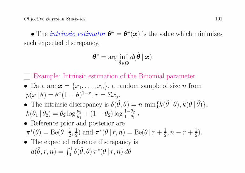
Objective Bayesian Statistics 101
• The intrinsic estimator θ∗ = θ∗(x) is the value which minimizes
such expected discrepancy,
θ∗ = arg infθ∈Θ
d(θ |x).
Example: Intrinsic estimation of the Binomial parameter
• Data are x = x1, . . . , xn, a random sample of size n from
p(x | θ) = θx(1− θ)1−x, r = Σxj.
• The intrinsic discrepancy is δ(θ, θ) = n mink(θ | θ), k(θ | θ),k(θ1 | θ2) = θ2 log θ2
θ1+ (1− θ2) log 1−θ2
1−θ1,
• Reference prior and posterior are
π∗(θ) = Be(θ | 12,
12) and π∗(θ | r, n) = Be(θ | r + 1
2, n− r + 12).
• The expected reference discrepancy is
d(θ, r, n) =∫ 1
0 δ(θ, θ) π∗(θ | r, n) dθ
Objective Bayesian Statistics 102
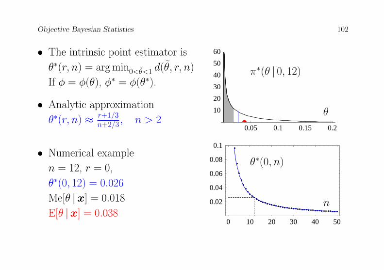
• The intrinsic point estimator is
θ∗(r, n) = arg min0<θ<1 d(θ, r, n)
If φ = φ(θ), φ∗ = φ(θ∗).
0 10 20 30 40 50
0.02
0.04
0.06
0.08
0.1
0.05 0.1 0.15 0.2
10
20
30
40
50
60
n
θ∗(0, n)
θ
π∗(θ | 0, 12)
• Analytic approximation
θ∗(r, n) ≈ r+1/3n+2/3, n > 2
• Numerical example
n = 12, r = 0,
θ∗(0, 12) = 0.026
Me[θ |x] = 0.018
E[θ |x] = 0.038
Objective Bayesian Statistics 103
Intrinsic estimation of the normal variance
• Given a random sample x1, . . . , xn from a normal distribution
N(x |µ, σ), the intrinsic (invariant) point estimator of the normal stan-
dard deviation σ is
σ∗ ≈ n
n− 1s, ns2 =
n∑i=1
(xi − x)2.
• Hence, the intrinsic point estimator of the normal variance σ2 is
σ2∗ ≈ n
n− 1
ns2
n− 1,
larger than both the mle s2 and the unbiased estimator ns2/(n− 1).
Objective Bayesian Statistics 104
Intrinsic region (interval) estimation
• The intrinsic q-credible region R∗(q) ⊂ Θ is that q-credible refer-
ence region which corresponds to minimum expected intrinsic loss:
(i)∫R∗(q) π(θ |x) dθ = q
(ii) ∀θi ∈ R∗(q), ∀θj /∈ R∗(q), d(θi |x) < d(θj |x)
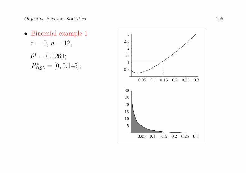
• In one parameter problems, plotting together, with the same scale
for θ, both the posterior distribution π(θ |x) and the posterior ex-
pected intrinsic loss d(θi |x) provides an illuminating comprehensive
view, on a probability density and a loss scale respectively, of the in-
ferential implications of the data x on the value of the parameter θ.
This is illustrated below with two examples from binomial data.
Objective Bayesian Statistics 105
• Binomial example 1
r = 0, n = 12,
θ∗ = 0.0263;
R∗0.95 = [0, 0.145];
0.05 0.1 0.15 0.2 0.25 0.3
5
10
15
20
25
30
0.05 0.1 0.15 0.2 0.25 0.3
0.5
1
1.5
2
2.5
3
Objective Bayesian Statistics 106
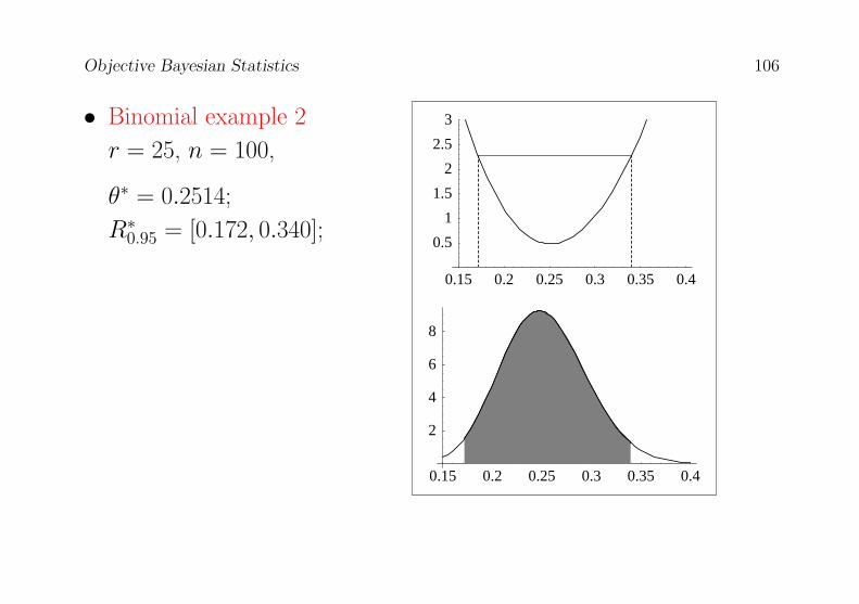
• Binomial example 2
r = 25, n = 100,
θ∗ = 0.2514;
R∗0.95 = [0.172, 0.340];
0.15 0.2 0.25 0.3 0.35 0.4
2
4
6
8
0.15 0.2 0.25 0.3 0.35 0.4
0.5
1
1.5
2
2.5
3
Objective Bayesian Statistics 107
Precise Hypothesis Testing
• The intrinsic reference test criterion is the Bayes test criterion
which corresponds to the use of the intrinsic loss and the reference
prior:
Reject θ0 (and only if) the expected reference posterior intrinsic
discrepancy d(θ0 |x) is too large,
d(θ0 |x) =∫
Θ δ(θ0,θ) π(θ |x) dθ > d∗, for some d∗ > 0.
Calibration of the test
• The intrinsic reference test statistic d(θ0 |x) is the reference poste-
rior expected value of the intrinsic discrepancy between p(x |θ0) and
p(x |θ), which is the minimum expected log-likelihood ratio against
the hypothesis that θ = θ0. Thus,
Objective Bayesian Statistics 108
A reference test statistic value d(θ0 |x) of, say, log(10) = 2.303
implies that, given data x, the average value of the likelihood ratio
against the hypothesis, p(x |θ)/p(x |θ0), is expected to be about 10,
suggesting some mild evidence against θ0.
Similarly, a value d(θ0 |x) of log(100) = 4.605 indicates an aver-
age value of the likelihood ratio against θ0 of about 100, indicating
rather strong evidence against the hypothesis, and log(1000) = 6.908,
a rather conclusive likelihood ratio against the hypothesis the of about
1000.
• Notice that the test statistic d(θ0 |x) is deemed to be large because
it directly indicates that given the data, the true model p(x |θ) is
probably rather different from p(x |θ0). This has nothing to do with
the sampling properties of d(θ0 |x) under p(x |θ0).
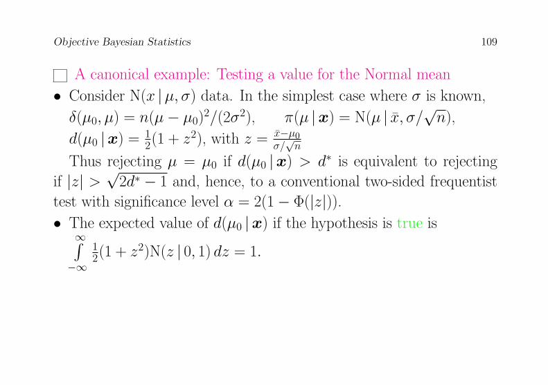
Objective Bayesian Statistics 109
A canonical example: Testing a value for the Normal mean
• Consider N(x |µ, σ) data. In the simplest case where σ is known,
δ(µ0, µ) = n(µ− µ0)2/(2σ2), π(µ |x) = N(µ | x, σ/√n),
d(µ0 |x) = 12(1 + z2), with z = x−µ0
σ/√n
Thus rejecting µ = µ0 if d(µ0 |x) > d∗ is equivalent to rejecting
if |z| >√
2d∗ − 1 and, hence, to a conventional two-sided frequentist
test with significance level α = 2(1− Φ(|z|)).• The expected value of d(µ0 |x) if the hypothesis is true is∞∫−∞
12(1 + z2)N(z | 0, 1) dz = 1.
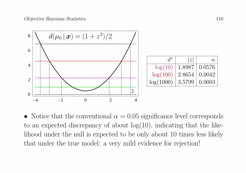
Objective Bayesian Statistics 110
-4 -2 0 2 40
2
4
6
8
d∗ |z| α
log(10) 1.8987 0.0576log(100) 2.8654 0.0042
log(1000) 3.5799 0.0003
z
d(µ0 |x) = (1 + z2)/2
• Notice that the conventional α = 0.05 significance level corresponds
to an expected discrepancy of about log(10), indicating that the like-
lihood under the null is expected to be only about 10 times less likely
that under the true model: a very mild evidence for rejection!
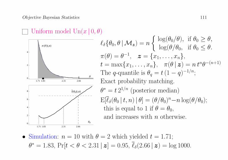
Objective Bayesian Statistics 111
Uniform model Un(x | 0, θ)
1.71 1.83 2.31 2.660
2
4
Π HΘ Èt,nL
Θ
1.71 1.83 2.31 2.660
2
4
6
8 lHΘ0Èt,nL
Θ0
`δθ0, θ |Mz) = n
log(θ0/θ), if θ0 ≥ θ,
log(θ/θ0, if θ0 ≤ θ.
π(θ) = θ−1, z = x1, . . . , xn,t = maxx1, . . . , xn, π(θ | z) = n tnθ−(n+1)
The q-quantile is θq = t (1− q)−1/n;
Exact probability matching.
θ∗ = t 21/n (posterior median)
E[`δ(θ0 | t, n) | θ] = (θ/θ0)n−n log(θ/θ0);
this is equal to 1 if θ = θ0,
and increases with n otherwise.
• Simulation: n = 10 with θ = 2 which yielded t = 1.71;
θ∗ = 1.83, Pr[t < θ < 2.31 | z] = 0.95, `δ(2.66 | z) = log 1000.
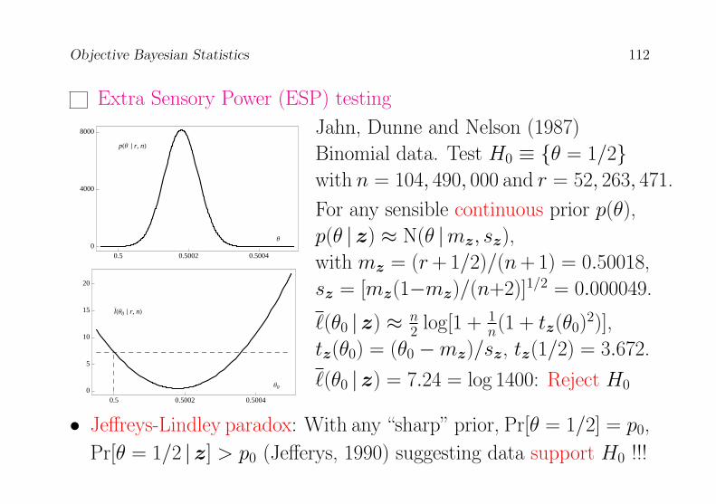
Objective Bayesian Statistics 112
Extra Sensory Power (ESP) testing
0.5 0.5002 0.50040
4000
8000
pHΘ È r, nL
Θ
0.5 0.5002 0.50040
5
10
15
20
lHΘ0 È r, nL
Θ0
Jahn, Dunne and Nelson (1987)
Binomial data. Test H0 ≡ θ = 1/2with n = 104, 490, 000 and r = 52, 263, 471.
For any sensible continuous prior p(θ),
p(θ | z) ≈ N(θ |mz, sz),
with mz = (r+ 1/2)/(n+ 1) = 0.50018,
sz = [mz(1−mz)/(n+2)]1/2 = 0.000049.
`(θ0 | z) ≈ n2 log[1 + 1
n(1 + tz(θ0)2)],
tz(θ0) = (θ0 −mz)/sz, tz(1/2) = 3.672.
`(θ0 | z) = 7.24 = log 1400: Reject H0
• Jeffreys-Lindley paradox: With any “sharp” prior, Pr[θ = 1/2] = p0,
Pr[θ = 1/2 | z] > p0 (Jefferys, 1990) suggesting data support H0 !!!
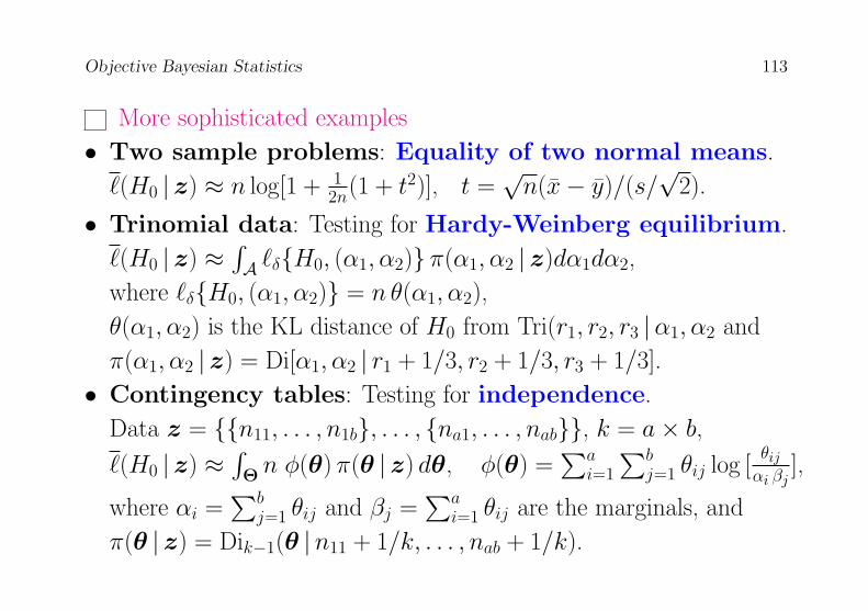
Objective Bayesian Statistics 113
More sophisticated examples
• Two sample problems: Equality of two normal means.
`(H0 | z) ≈ n log[1 + 12n(1 + t2)], t =
√n(x− y)/(s/
√2).
• Trinomial data: Testing for Hardy-Weinberg equilibrium.
`(H0 | z) ≈∫A `δH0, (α1, α2) π(α1, α2 | z)dα1dα2,
where `δH0, (α1, α2) = n θ(α1, α2),
θ(α1, α2) is the KL distance of H0 from Tri(r1, r2, r3 |α1, α2 and
π(α1, α2 | z) = Di[α1, α2 | r1 + 1/3, r2 + 1/3, r3 + 1/3].
• Contingency tables: Testing for independence.
Data z = n11, . . . , n1b, . . . , na1, . . . , nab, k = a× b,`(H0 | z) ≈
∫Θ n φ(θ) π(θ | z) dθ, φ(θ) =
∑ai=1
∑bj=1 θij log [
θijαi βj
],
where αi =∑b
j=1 θij and βj =∑a
i=1 θij are the marginals, and
π(θ | z) = Dik−1(θ |n11 + 1/k, . . . , nab + 1/k).
Objective Bayesian Statistics 114
Basic References(In chronological order)
Available on line from www.uv.es/bernardo
Bernardo, J. M. (1979). Reference posterior distributions for Bayesian
inference. J. Roy. Statist. Soc. B 41, 113–147 (with discussion).
Berger, J. O. and Bernardo, J. M. (1992). On the development of
reference priors. Bayesian Statistics 4 (J. M. Bernardo, J. O. Ber-
ger, A. P. Dawid and A. F. M. Smith, eds.) Oxford: University
Press, 35–60 (with discussion).
Bernardo, J. M. (1997). Noninformative priors do not exist J. Statist.
Planning and Inference 65, 159–189 (with discussion).
Bernardo, J. M. and Rueda, R. (2002). Bayesian hypothesis testing:
A reference approach. Internat. Statist. Rev. 70, 351–372.
Objective Bayesian Statistics 115
Bernardo, J. M. (2005a). Reference analysis. Bayesian Thinking:
Modeling and Computation, Handbook of Statistics 25 (Dey,
D. K. and Rao, C. R., eds). Amsterdam: Elsevier, 17–90.
Bernardo, J. M. (2005b). Intrinsic credible regions: An objective
Bayesian approach to interval estimation. Test 14, 317–384 (with
discussion).
Berger, J. O. (2006). The case for objective Bayesian analysis. Bayesian
Analysis 1, 385–402 and 457–464, (with discussion).
Bernardo, J. M. (2007). Objective Bayesian point and region estima-
tion in location-scale models. Sort 31, 3–44, (with discussion).
Bernardo, J. M. (2009). Statistics: Bayesian methodology in statis-
tics. Comprehensive Chemometrics (S. Brown, R. Tauler and R.
Walczak eds.) Oxford: Elsevier, 213–245.
Objective Bayesian Statistics 116
Berger, J. O., Bernardo, J. M. and Sun, D. (2009a). The formal defi-
nition of reference priors. Ann. Statist. 37, 905–938.
Berger, J. O., Bernardo, J. M. and Sun, D. (2009b). Natural induction:
An objective Bayesian approach. Rev. Acad. Sci. Madrid, A
103, 125–159 (invited paper with discussion).
Bernardo, J. M. (2011). Integrated objective Bayesian estimation and
hypothesis testing. Bayesian Statistics 9 (J. M. Bernardo, M. J.
Bayarri, J. O. Berger, A. P. Dawid, D. Heckerman, A. F. M. Smith
and M. West, eds). Oxford: Oxford University Press, 1–68 (with
discussion).
Objective Bayesian Statistics 117
Bernardo, J. M. (2011). Bayes and discovery: Objective Bayesian
hypothesis testing. PHY- STAT 2011 Workshop on Statistical
Issues Related to Discovery Claims in Search Experiments and
Unfolding (H. B. Prosper and L. Lyons, eds.). Geneva: CERN,
27-49 (with discussion).
Berger, J. O., Bernardo, J. M. and Sun, D. (2012). Objective priors for
discrete parameter spaces. J. Amer. Statist. Assoc. 107, 636–648
Berger, J. O., Bernardo, J. M. and Sun, D. (2014). Overall objective
priors. Bayesian Analysis (forthcoming, with discussion).
www.uv.es/bernardo