An introduction to probabilistic automata

Marielle Stoelinga�Department of Computer Engineering

University of California at Santa Cruz, CA 95064, USAmarielle@cse.ucsc.edu

Abstract

This paper provides an elementary introduction to the probabilistic automaton (PA) model, whichhas been developed by Segala. We describe how distributed systems with discrete probabilities canbe modeled and analyzed by means of PAs. We explain how the basic concepts for the analysis ofnonprobabilistic automata can be extended to probabilistic systems. In particular, we treat the parallelcomposition operator on PAs, the semantics of a PA as a set of trace distributions, an extension of thePA model with time and simulation relations for PAs. Finally, we give an overview of various other statebased models that are used for the analysis of probabilisticsystems.

1 Introduction

Probabilistic Automata (PAs) constitute a mathematical framework for the specification and analysis ofprobabilistic systems. They have been developed by Segala [Seg95b, SL95, Seg95a] and serve the pur-pose of modeling and analyzing asynchronous, concurrent systems with discrete probabilistic choice in aformal and precise way. Examples of such systems are randomized, distributed algorithms (such as therandomized dining philosophers [LR81]), probabilistic communication protocols (such as the IEEE 1394Root Contention protocol [IEE96]) and the Binary Exponential Back Off protocol, see [Tan81]); and faulttolerant systems (such as unreliable communication channels).

PAs are based on state transition systems and make a clear distinction betweenprobabilisticandnon-deterministic choice. We will go into the differences and similarities between both types of choices laterin this paper. As subsume nonprobabilistic automata, Markov chains and Markov decision processes. ThePA framework does not provide any syntax, but several syntaxes have been defined on top of it to facilitatethe modeling of a system as a PA. Properties of probabilisticsystems that can be established formally us-ing PAs include correctness and performance issues, such as: Is the probability that an error occurs smallenough (e.g.< 10�9)? Is the average time between two subsequent failures largeenough? What is theminimal probability that the system responds within 3 seconds?

A PA has a well–defined semantics as a set oftrace distributions. The parallel composition operatorkallows one to construct a PA from several component PAs running in parallel, thus keeping system modelsmodular. PAs have been extended with time in order to model and reason about time.

The aim of this paper is to explain the basic ideas behind PAs and their behavior in an intuitive way.Our explanation focuses on the differences and similarities with nonprobabilistic automata.

Organization of the paper This paper is organized as follows. Section 2 introduces theprobabilisticautomaton model and Section 3 treats its behavior (semantics). Then Sections 4 and 5 are concernedrespectively with implementation and simulation relations for PAs. In Section 6, we give several othermodels dealing with probabilistic choice and finally, Section 7 presents a summary of the paper.�This paper is a revised version of a Chapter 2 in [Sto02], which was written while the author working at the Computing ScienceInstitute, University of Nijmegen, the Netherlands.

1

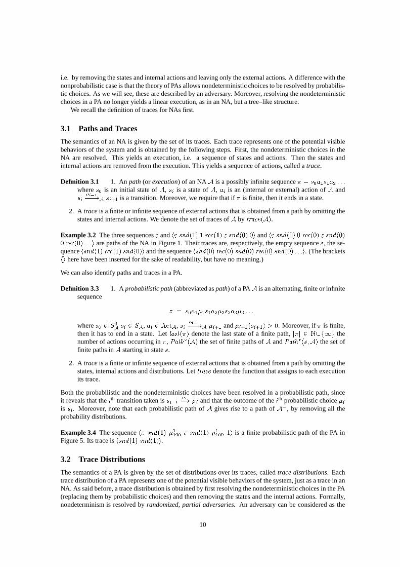
0 " 1n � ��� �� n� -snd(0) snd(1)- �re (0) re (1)Figure 1: A channel automaton

2 The Probabilistic Automaton Model

Basically, a probabilistic automaton is just an ordinary automaton (also calledlabeled transition systemor state machine) with the only difference that the target of a transition is aprobabilistic choice overseveral next states. Before going into the details of this, we briefly recall the notion of a nonprobabilisticautomaton, which also known as a state machine, a labeled transition system, or a state transition system.

2.1 Nonprobabilistic Automata

An nonprobabilistic automaton, abbreviated NA, is a structure consisting ofstatesand transitions; thelatter are also calledsteps. The states of an NA represent the states in the system that ismodeled. Oneor more states are designated asstart states, representing the initial configuration of the system. Thetransitions in the NA represent changes of the system statesand are labeled by actions. Thus, the transitions a�! s0 represents that, being in states, the system can move via ana–action to another states0. Theaction labels are partitioned intointernal andexternalactions. The former represent internal computationsteps of the automaton and are not visible to the automaton’senvironment. We often use the symbol� todenote an internal action. The external actions are visiblefor the automaton’s environment and are usedfor interaction with it. This will be explained in more detail in Section 2.4.

Example 2.1 Consider the NA in Figure 1. It models a 1–place buffer used asa communication channelfor the transmission of bits between two processes. The states", 0 and1 represent respectively the channelbeing empty, the channel containing the bit 0 and the channelcontaining a 1. Initially, the channel is empty(denoted by the double circle in the picture). The transitions" snd(i)����! i represent the sender process (notdepicted here) sending the biti to the channel. Similarly, the transitionsi re (i)���! " represent the deliveryof the bit at the receiver process. Notice that the transition labeledsnd(i) represents the sending of abit by the sender, which is the receipt of a bit by the communication channel. Similarly, the receipt of abit at the receiving process corresponds to the sending of a bit by the channel, which is modeled by there (i)–transitions.

It is natural that the actionssnd(0), re (0), snd(1) andre (1) in this NA are external, since these areused for communication with the environment.

Thus, the notion of an NA can be formalized as follows.

Definition 2.2 An NA A consists of four components:

1. A setSA of states,

2. a nonempty setS0A � SA of start states,

3. An action signaturesigA = (VA; IA), consisting ofexternal (visible)and internal actionsrespec-tively. We requireVA andIA to be disjoint and define the set ofactionsasA tA = VA [ IA.

4. atransition relation�A � SA �A tA � SA.

We writes a�!A s0, or s a�! s0 if A is clear from the context, for(s; a; s0) 2 �A. Moreover, we say that theactiona is enabledin s, if s has an outgoing transition labeled bya.

Several minor variations of this definition exist. Some definitions require, for instance, a unique startstate rather than a set of start states or allow only a single internal action, rather than a set of these. In theI/O automaton model [LT89], external actions are divided into input andoutputactions. Input actions, not

2

being under the control of the NA, are required to be enabled in any state. The basic concepts are similarfor the various definitions.

2.1.1 Nondeterminism

Nondeterministic choices can be specified in an automaton byhaving several transitions leaving from thesame state. Nondeterminism is used when we wish to incorporate several potential system behaviors in amodel. Hoare [Hoa85] phrases it as follows:

There is nothing mysterious about nondeterminism, it arises from the deliberated decision toignore the factors which influence the selection.

Nondeterministic choices are often divided into external and internal nondeterministic choices.Exter-nal nondeterministic choices are choices that can be influencedby the environment. Since interaction withthe environment is performed via external actions, external nondeterministic behavior is specified by hav-ing several transitions with different labels leaving fromthe same state.Internalnondeterministic choicesare choices that are made by the automaton itself, independent of the environment. These are modeled byinternal actions or by including several transitions with the same labels leaving from the same state. In theliterature, the word nondeterminism sometimes refers to what we call internal nondeterminism.

As pointed out by [Seg95b, Alf97], nondeterminism is essential for the modeling of the followingphenomena.

Scheduling freedomWhen a system consists of several components running in parallel, we often do notwant to make any assumptions on the relative speeds of the components, because we want the application towork no matter what these relative speeds are. Therefore, nondeterminism is essential to define the parallelcomposition operator (see Definition 2.13), where we model the choice of which automaton in the systemtakes the next step as an (internal or external) nondeterministic choice.

Implementation freedom Automata are often used to represent a specification. Good software engineer-ing practice requires the specification to describeswhat the system should do, nothow it should be im-plemented. Therefore, a specification usually leaves room for several alternative implementations. Sinceit does not matter for the correct functioning of the system which of the alternatives is implemented, suchchoices are also represented by (internal or external) nondeterminism.

External environment An automaton interacts with its environment via its external actions. When mod-eling a system, we do not wish to stipulate how the environment will behave. Therefore the possibleinteractions with the environment are modeled by (external) nondeterministic choices.

Incomplete information Sometimes it is not possible to obtain exact information about the system to bemodeled. For instance, one might not know the exact durationof or — in probabilistic systems — the exactprobability of an event, but only a lower and upper bound. In that case, one can incorporate all possiblevalues by a nondeterministic choice. This is appropriate since we consider a system to be correct if itbehaves as desired no matter how the nondeterministic choices are resolved.

Example 2.3 In the state", the channel NA in Figure 1 contains an external nondeterministic choicebetween the actionssnd(0) andsnd(1). This models a choice to be resolved by the environment (in thiscase a sender process) which decides which bit to sent. Nondeterministic choices modeling implementationfreedom, scheduling freedom, and incomplete information are given in Examples 2.9 and 2.14.

2.2 Probabilistic Automata

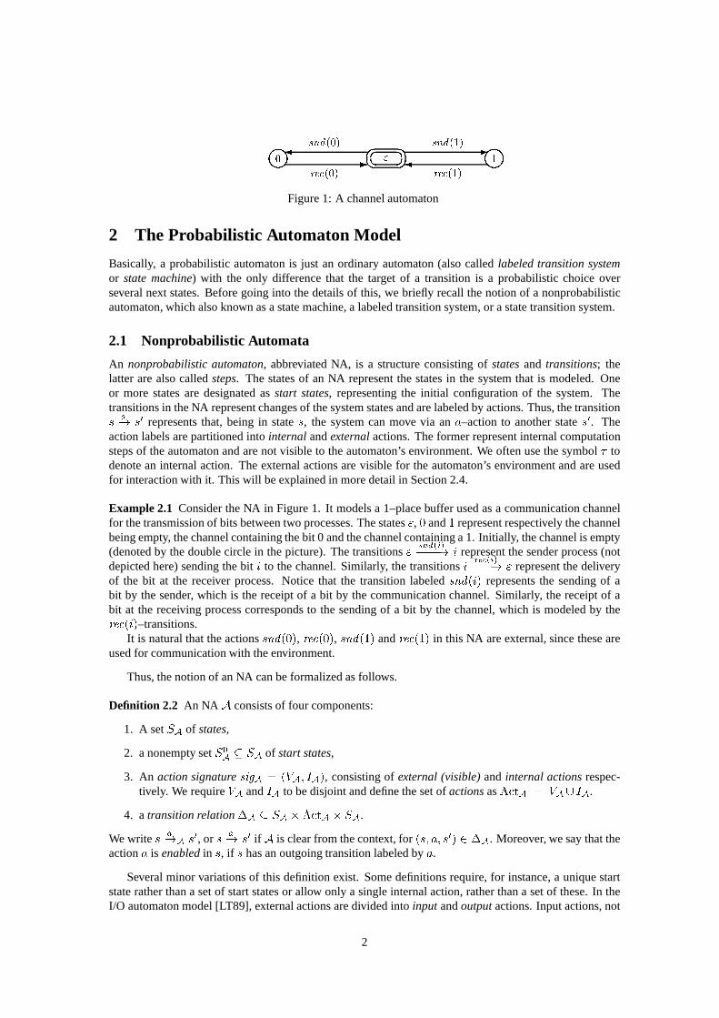
As said before, the only difference between a nonprobabilistic and a probabilistic automaton is that thetarget of a transition in the latter is no longer a single state, but is a probabilistic choice over several nextstates. For instance, a transition in a PA may reach one statewith probability 12 and another one withprobability 12 too. In this way, we can represent a coin flip and a dice roll, see Figure 2.

3

hd tl

s ipk kk� JJJ12 12hd tl

s ipk kk� JJJ13 23 16 16 16 16 16 16s1 2 3 4 5 6

rollk k k k k kk�����= ������� JJJZZZZ~HHHHHHjFigure 2: Transitions representing a fair coin flip, an unfair coin flip and a fair dice roll.0 " 1n � ��� �� n� -� �?110099100 snd(1)� �?snd(0) 1100 99100- �re (0) re (1)

Figure 3: A lossy channel PA

Thus, a transition in a PA relates a state and an action to aprobability distributionover the set ofstates. A probability distribution over a setX is a function� that assigns a probability in[0; 1℄ to eachelement ofX , such that the sum of the probabilities of all elements is 1. LetDistr(X) denote the set ofall probability distributions overX . Thesupportof � is the setfx 2 X j �(x) > 0g of elements that areassigned a positive probability. IfX = fx1; x2; : : :g, then we often write the probability distribution� asfx1 7! �(x1); x2 7! �(x2) : : :g and we leave out the elements that have probability 0.

Example 2.4 Let the set of states be given bys, hd , tl , 1, 2, 3, 4, 5 and6. The transitions in Figure 2 arerespectively given by s ip��! fhd 7! 12 ; tl 7! 12g;s ip��! fhd 7! 13 ; tl 7! 23g ands roll��! f1 7! 16 ; 2 7! 16 ; 3 7! 16 ; 4 7! 16 ; 5 7! 16 ; 6 7! 16g:Note that we have left out many elements with probability 0, for instance the states is reached withprobability 0 by each of the transitions above. Moreover, each of the three pictures in Figure 2 representsa single transition, where several arrows are needed to represent the probabilistic information.

The definition of a PA is now given as follows.

Definition 2.5 A PAA consists of four components:

1. A setSA of states,

2. a nonempty setS0A � SA of start states,

3. An action signaturesigA = (VA; IA), consisting ofexternalandinternal actionsrespectively. WerequireVA andIA to be disjoint and define the set ofactionsasA tA = VA [ IA.

4. atransition relation�A � SA �A tA �Distr(SA).Again, we writes a�!A � for (s; a; �) 2 �A. Furthermore, we simply writes a�!A s0 for s a�!A fs0 7! 1g.

Obviously, the definition of PAs gives rise to the same variations as the definition of NAs.

Example 2.6 The PA in Figure 3 represents the same 1–place communicationchannel as the NA in Fig-ure 1, except that now the channel is lossy: a bit sent to the channel is lost with a probability of1100 . Byconvention, the transitionsi re (i)���! " reach the state" with probability 1.

4

e ee� JJJ12 12snd(0) snd(1) e ee ee � JJJ? ?12 12snd(0) snd(1)�Figure 4: Modeling multi–labeled transitions in a PA

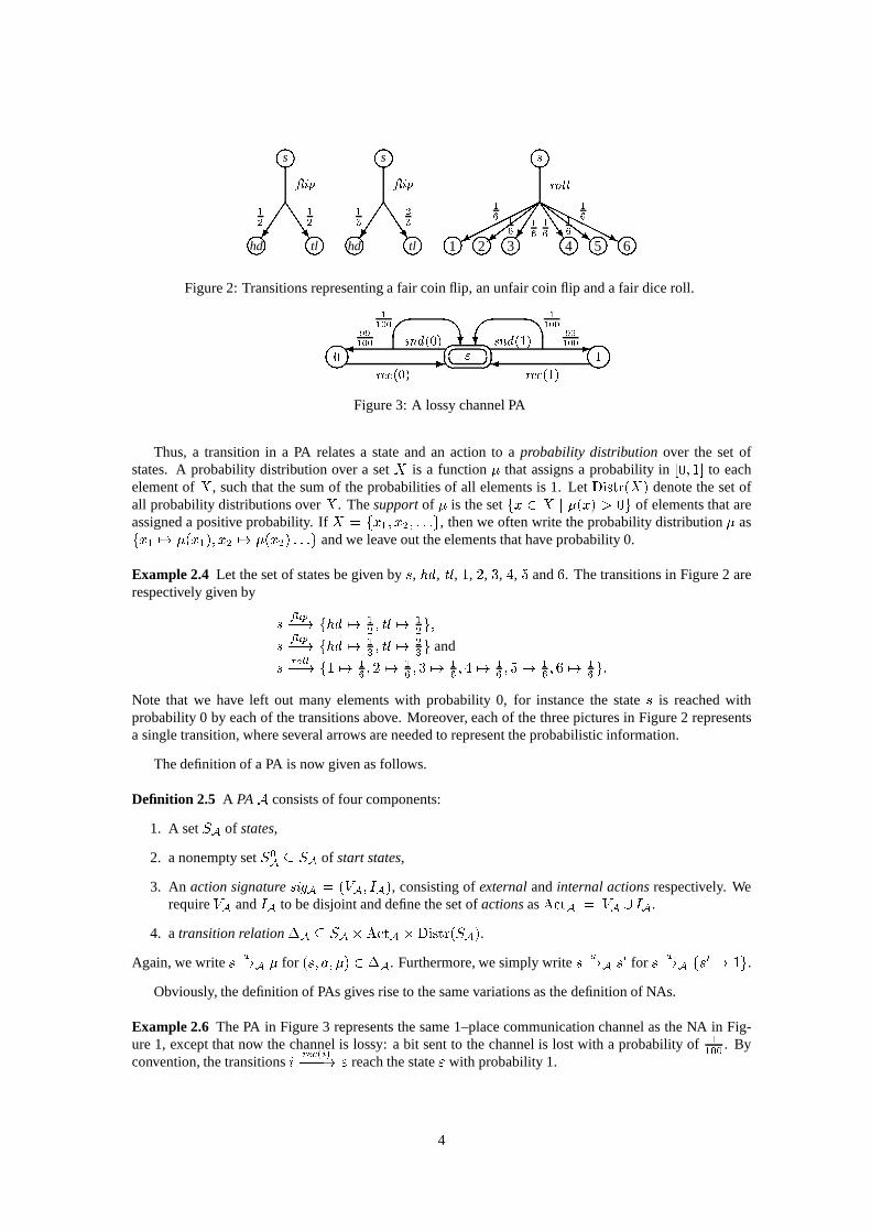
Remark 2.7 Note that each transition in a PA is labeled with a single action. The system depicted on theleft in Figure 4 models a process sending the bits 0 and 1 each with probability 12 . However, this system isnot a PA, because two actions appear in the same transition. Rather, a PA model of such a process is shownon the right of Figure 4.

There is, however, a multilabeled version of the PA model, see Section 2.5. That model is technicallymore complex and, in practice, the PA model is expressive enough.

Remark 2.8 The nonprobabilistic automata can be embedded in the probabilistic ones by viewing eachtransitions a�! s0 in an NA as the transitions a�! fs0 7! 1g in a PA. Conversely, each PAA can be “deprob-abilized,” yielding an NAA�, by forgetting the specific probabilistic information and by only retainingwhether a state can be reached with a positive probability. Precisely,s a�! s0 is a transition inA� if andonly if there is a transitions a�! � in A with �(s0) > 0.

2.2.1 Probabilistic versus nondeterministic choice

One can specify nondeterministic choices in a PA in exactly the same way as in a NA, viz. by having internaltransitions or by having several transitions leaving from the same state. Also the distinction betweenexternal and internal nondeterminism immediately carriesover to PAs. Hence, the probabilistic choices arespecifiedwithin the transitions of a PA and the nondeterministic choicesbetweenthe transitions (leavingfrom the same state) of a PA.

Section 2.1.1 has pointed out the need for nondeterministicchoices in automata, namely to modelscheduling freedom, implementation freedom, the externalenvironment and incomplete information. Thesearguments are still valid in the presence of probabilistic choice. In particular,nondeterminism cannot bereplaced by probabilityin these cases. As mentioned, nondeterminism is used if we deliberately decide notto specify how a certain choice is made, so in particular we donot want to specify a probability mechanismthat governs the choice. Rather, we use a probabilistic choice if the event to be modeled has really allthe characteristics of a probabilistic choice. For instance, the outcome of a coin flip, random choices inprogramming languages, and the arrivals of consumers in a shop. Thus, probability and nondeterminismare two orthogonal and essential ingredients in the PA model.

An important difference between probabilistic and nondeterministic choice is that the former are gov-erned by a probability mechanism, whereas the latter are completely free. Therefore, probabilistic choicesfulfill the laws from probability theory, and in particular the law of large numbers. Informally, this lawstates that if the same random choice is made very often, the average number of times that a certain eventoccurs is approximately (or, more precisely, it converges to) its expected value. For instance, if we flip afair coin one hundred times, it is very likely that about halfof the outcomes is heads and the other halfis tails. If, on the other hand, we make a nondeterministic choice between two events, then we cannotquantify the likelihood of the outcomes. In particular, we cannot say that each of the sequences is equallylikely, because this refers to a probabilistic choice!

The following example illustrates the combination of nondeterministic choice and probabilistic choice.

5

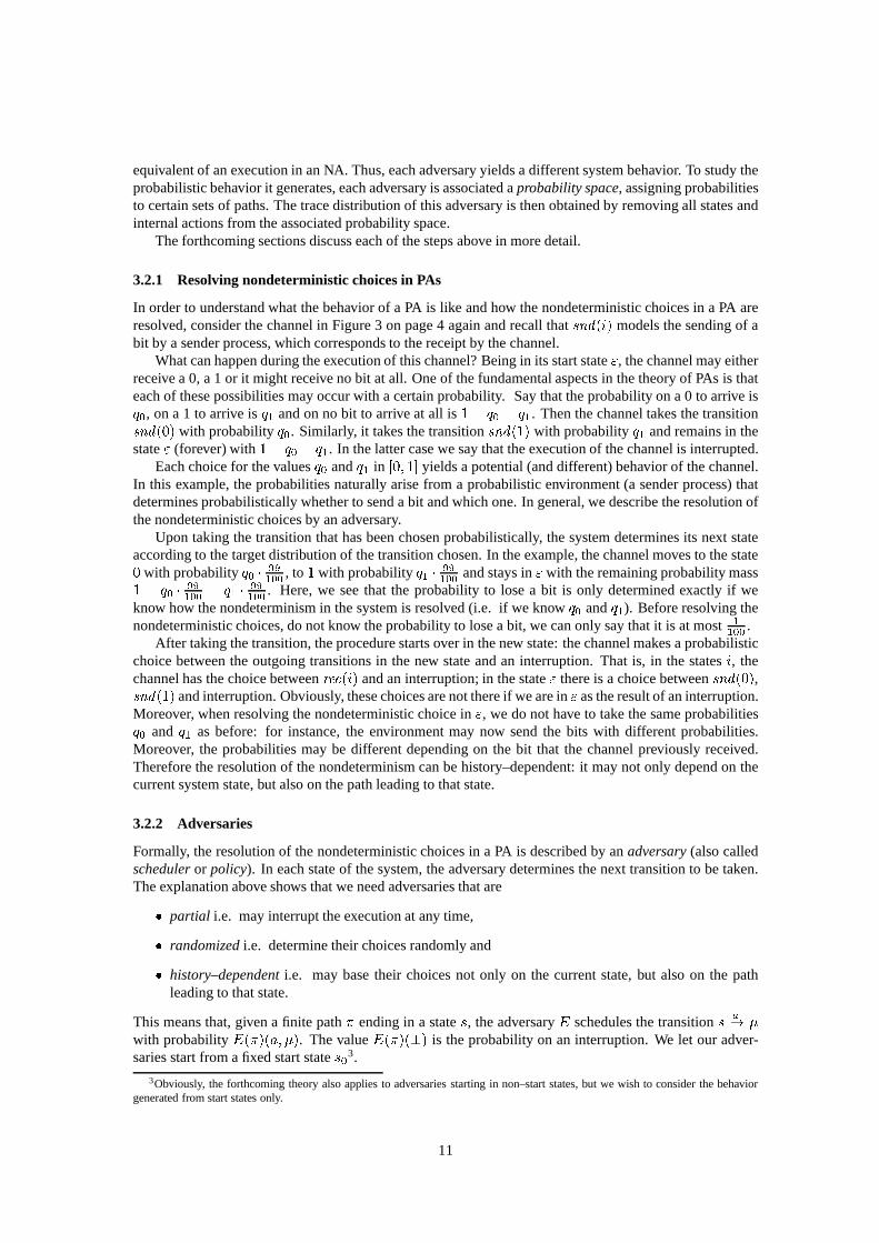
0 " 1n � ��� �� n� -' $?re (0) ' $re (1)� �?110099100 snd(1)� �?snd(0) 1100 99100� � �6snd(0)1200199200 snd(1)snd(0) snd(1) -� �6 1200 199200Figure 5: A lossy channel PA with partially unknown probabilities

Example 2.9 Like in Figure 3, the PA in Figure 5 also represents a faulty communication channel. Thedifference with the PA in Figure 3 is that, here, we do not knowthe probability that a bit is lost exactly.Depending on which transition is taken, it can be1200 or 1100 . However, we will see in Section 3 that thisprobability can in fact have any value between1200 and 1100 . Thus, the nondeterministic choice between thetwo send(i) transitions is used here to represent incomplete information about exact probabilities.

This PA can also be considered as the specification of a system, where the nondeterministic choicerepresents implementation freedom: It requires that in an implementation the probability to lose a messageis at most 1100 and at least 1200 . (The latter might be a bit awkward in practice.)

For future use, define distributions�ix and the transitions�ix by�ix = " snd(i)����! �ix; �ix = f" 7! 1x ; i 7! x�1x g:wherex = 100; 200 andi = 0; 1. Thus, the superscripts denote the bit and the subscripts the probability.

Finally, we remark that the philosophical debate on the nature of nondeterminism choice and probabilityhas not ended. In this paper, we take a practical standpoint and postulate that both types of choices areappropriate for describing and predicting certain phenomena in system behavior. For more information onthe philosophical issues arising in the area of probabilitytheory, the reader is referred to [Coh89].

2.3 Timing

Timing can be incorporated in the PA model in a similar way as in the NA model (c.f. the “old fashionedrecipe for time” [AL92]). Aprobabilistic timed automaton (PTA)is a PA with time passage actions. Theseare actionsd 2 R>0 that indicate the passage ofd time units. While time elapses, no other actionstake place and, in the PTA approach, time advances deterministically. So, in particular, no (internally)nondeterministic or probabilistic choices can be specifiedwithin time passage actions, see requirements 1and 2 in the definition below. The third condition below, Wang’s Axiom [Yi90], requires that, while timeadvances, the state of the PTA is well–defined at each point intime and that, conversely, two subsequenttime passage actions can be combined into a single one.

The PTA model presented here is a simplification of the one [Seg95b], which is based on a generaliza-tion of Wang’s axiom.

Definition 2.10 A PTAA is a PA enriched with a partition ofA t nf�g into a set ofdiscrete actionsA tDand the setR>0 of positive real numbers ortime–passage actions. We require1 that, for alls; s0; s00 2 SAandd; d0 2 R>0 with d0 < d,

1. each transition labeled with a time–passage action leadsto a distribution that chooses one elementwith probability 1,

2. (Time determinism) ifs d�!A s0 ands d�!A s00 thens0 = s00.3. (Wang’s Axiom)s d�!A s0 iff 9s00 : s d0�!A s00 ands00 d�d0���!A s0.

1For simplicity the conditions here are slightly more restrictive than those in [LV96].

6

s0; 0 s2; 0s1; 0 s2; 2s1; 1 s4; 2s3; 1� � � �� � � �� � � �� �HHHj���* -- --� 12 aa1212Figure 6: A part of a PTA

As PTAs are a special kind of PAs, we can use the notions definedfor PAs also for PTAs.By letting time pass deterministically, PTAs treat probabilistic choice, nondeterministic choice and time

passage as orthogonal concepts, which leads to a technically clean model. Example 2.11 below shows thatdiscrete probabilistic choices over time can be encoded in PTAs via internal actions. Nondeterministicchoices over time can be encoded similarly: just replace theprobabilistic choice in the example by anondeterministic one. Thus, although we started from a deterministic view on time, nondeterminism andprobabilistic choices over time sneak in via a back door. Theadvantage of the PTA approach is thatwe separate concerns by specifying one thing at the time: time passage or probabilistic/nondeterministicchoice.

Example 2.11 We can use a PTA to model a system that decides with an internalprobabilistic choicewhether to wait a short period (duration one time unit) or a long period (two time units) before performingana action. This PTA is partially given in Figure 6, where the second element of each state records theamount of time that has elapsed. Note that there are uncountably many transitions missing in the picture,for instance the transitions(s1; 0) 0:2��! (s1; 0:2) and (s1; 0:2) 0:5��! (s1; 0:7), see Wang’s Axiom in thepreceding definition. The full transition relation is givenby(s0; 0) ��! f(s1; 0) 7! 12 ; (s2; 0) 7! 12g;(s1; d) d0�! (s1; d+ d0); if d+ d0 � 1;(s2; d) d0�! (s2; d+ d0); if d+ d0 � 2;(s1; 1) a�! (s3; 1);(s2; 2) a�! (s4; 1):Continuous distributions over time can of course not be encoded in a PTA, since such distributions cannotbe modeled in the PA model anyhow. There are various other models combining time and probability, seeSection 6, including models dealing with continuous distributions over time.

Moreover, there is a second model that extends PAs with nondeterministic timing. The automata in-troduced in [KNSS01] — also called PTAs — augment the classical timed automata [AD94] with discreteprobabilistic choice. They allow timing constraints to be specified via real–valued clocks.

2.4 Parallel Composition

The parallel composition operatork allows one to construct a PA from several component PAs. Thismakessystem descriptions more understandable and enables component–wise design. The component PAs runin parallel and interact via their external actions. As before, the situation is similar to the nonprobabilisticcase.

Consider a composite PA that is built from two component PAs.Then the state space of the compositePA consists of pairs(s; t), reflecting that the first component is in states and the second in statet. If oneof the components can take a step, then so can the composite PA, wheresynchronizationon shared actionshas to be taken into account. This means that whenever one component performs a transition involving avisible actiona, the other one should do so simultaneously, provided thata is in its action set.

When synchronization occurs, both automata resolve their probabilistic choices independently, becausethe probability mechanisms used in different components are not supposed to influence each other. Thus,if the transitionss1 a�! �1 ands2 a�! �2 synchronize, then the state(s01; s02) is reached with probability�1(s01) ��2(s02). No synchronization is required for transitions labeled byan internal actiona 2 I nor forvisible actions which are not shared (i.e. present in only one of the automata). In this case, one componenttakes a transition, while the other remains in its current state with probability one. For instance, if the first

7

s0 s1 s2ni n n-snd(1)� �6 13 23 -a� �6 12 12Figure 7: A sender PA

component takes the transitions1 ��! �1 and the other one remains in the states2, then the probability toreach the state(s01; s2) by taking this transition equals�1(s01) and the probability to reach a state(s01; s02)with s02 6= s2 is zero.

To define the parallel composition, we need to define the probabilistic distribution arising from twoindependent probabilistic choices. Furthermore, we only take the parallel composition of PAs whose actionsignatures do not clash.

Notation 2.12 Let � be a probability distribution onX and� one onY . Define the distribution�� � onX � Y by (�� �)(x; y) = �(x) � �(y):Definition 2.13 We say that two PAsA andB arecompatibleif IA \A tB = A tA \ IB = ;. For twocompatible PAsA andB, theparallel compositionis the probabilistic automatonA k B defined by:

1. SAkB = SA � SB.

2. S0AkB = S0A � S0B.

3. sigAkB = (VA [VB; IA [ IB).4. �AkB is the set of transitions(s1; s2) a�! �1 � �2 such that at least one of the following requirements

is met.� a 2 VA \VB, s1 a�! �1 2 �A ands2 a�! �2 2 �B.� a 2 A tA nA tB or a 2 IA, ands1 a�! �1 2 �A and�2 = fs2 7! 1g.� a 2 A tB nA tA or a 2 IB, ands2 a�! �2 2 �B and�1 = fs1 7! 1g.Note that nondeterminism is essential in this definition.

Example 2.14 The system in Figure 7 represents a sender process. Its action set isfsnd(0); snd(1); ag.Figure 8 shows the parallel composition process of this process and the channel process in Figure 3.

2.5 Other Automaton Models with Nondeterminism and Discrete Probabilities

Below, we discuss the GPA model and the alternating model, which are two other automaton modelscombining discrete probabilities and nondeterminism. Both are equivalent to the PA model in some sense.

General probabilistic automata Segala [Seg95b] introduces a more general notion of probabilistic au-tomata, which we callgeneral probabilistic automata(GPAs)2. A GPA is the same as a PA, except that thetransitions have the typeS�Distr(A t � S [f?g). Thus, each transition chooses both the action and thenext state probabilistically. Moreover, it can choose to deadlock (?) with some probability. In the lattercase, no target state is reached. Figure 4 on page 5 shows a GPAthat is not a PA.

Problems arise when defining the parallel composition operator for arbitrary GPAs. The trouble comesfrom synchronizing transitions that have some shared actions and some actions which are not shared (see[Seg95b], Section 4.3.3).

The problem can be solved by imposing the I/O distinction on GPAs (c.f. the remark below Defini-tion 2.2). This distinction comes with the requirement thatinput actions are enabled in every state and

2Segala uses the word PA for what we call GPA and says simple PA to what we call PA.

8

s0; " s1; " s2; "s0; 1 s1; 1 s2; 1s0; 0 s1; 0 s2; 0� ��� �� � � � �� � � � � �� � � � � �-snd(1)� �6 �����������I 1300 230099300 198300

-a� �6 12 12-a� �6 12 12-a� �6 12 126re (0) 6re (0) 6re (0)?re (1) ?re (1) ?re (1)

Figure 8: Parallel composition

ee ee? ?HHHHHHj�������a b 1212 12 12 ee eeu u? ?? ?HHHHHHj�������a b 1212 12 12 ee eeu ������R��� ���Ra b1212Figure 9: A PA model and two alternating models equivalent toit

occur only on transitions labeled by a single action. This approach is followed in [WSS97] and in [HP00].Surprisingly, the latter reverses the role of input and output actions.

In our experience, many practical systems can be modeled conveniently with PAs (see Remark 2.7;deadlocks can be modeled by moving to a special deadlock state). Moreover, several notions have beenworked out for the PA model only. Therefore, this thesis deals with PAs rather than with GPAs.

Alternating model The alternating model, introduced by Hansson and Jonsson [Han94, HJ94], distin-guishes betweenprobabilistic and nondeterministic states. Nondeterministic states have zero or moreoutgoing transitions. These are labeled by actions and leadto a unique probabilistic state. Probabilisticstates have one or more outgoing transitions. These are labeled by probabilities and specify a probabilitydistribution over the nondeterministic states.

The alternating model and the PA model are isomorphic upto so-called strong bisimulation [LS91]. Thismeans that all notions defined on PAs that respect strong bisimulation can be translated into the alternatingmodel and vice versa.

In order to translate an alternating model into a PA, one removes all probabilistic states and contractseach ingoing transition of a probabilistic state with the probability distribution going out of that state,thus passing by the probabilistic state. Conversely, in order to translate a PA into an alternating model,one introduces an intermediate probabilistic state for each transition. The reason why this only yields anisomorphism upto bisimulation, rather than just an isomorphism, is illustrated in Figure 9.

3 The Behavior of Probabilistic Automata

This section defines the semantics of a PA as the set of its trace distributions. Each trace distribution isa probability space assigning a probability to certain setsof traces. The idea is that a trace distributionarises from resolving the nondeterministic choice first andby then abstracting from nonvisible elements,

9

i.e. by removing the states and internal actions and leavingonly the external actions. A difference with thenonprobabilistic case is that the theory of PAs allows nondeterministic choices to be resolved by probabilis-tic choices. As we will see, these are described by an adversary. Moreover, resolving the nondeterministicchoices in a PA no longer yields a linear execution, as in an NA, but a tree–like structure.

We recall the definition of traces for NAs first.

3.1 Paths and Traces

The semantics of an NA is given by the set of its traces. Each trace represents one of the potential visiblebehaviors of the system and is obtained by the following steps. First, the nondeterministic choices in theNA are resolved. This yields an execution, i.e. a sequence ofstates and actions. Then the states andinternal actions are removed from the execution. This yields a sequence of actions, called atrace.

Definition 3.1 1. An path(or execution) of an NAA is a possibly infinite sequence� = s0a1s1a2 : : :wheres0 is an initial state ofA, si is a state ofA, ai is an (internal or external) action ofA andsi ai+1���!A si+1 is a transition. Moreover, we require that if� is finite, then it ends in a state.

2. A traceis a finite or infinite sequence of external actions that is obtained from a path by omitting thestates and internal actions. We denote the set of traces ofA by tra e(A).

Example 3.2 The three sequences" andh" snd(1) 1 re (1) " snd(0) 0i andh" snd(0) 0 re (0) " snd(0)0 re (0) : : :i are paths of the NA in Figure 1. Their traces are, respectively, the empty sequence", the se-quencehsnd(1) re (1) snd(0)i and the sequencehsnd(0) re (0) snd(0) re (0) snd(0) : : :i. (The bracketshi here have been inserted for the sake of readability, but haveno meaning.)

We can also identify paths and traces in a PA.

Definition 3.3 1. A probabilistic path(abbreviated aspath) of a PAA is an alternating, finite or infinitesequence � = s0a1�1s1a2�2s2a3�3 : : :wheres0 2 S0A si 2 SA, ai 2 A tA, si ai+1���!A �i+1 and�i+1(si+1) > 0. Moreover, if� is finite,then it has to end in a state. Letlast(�) denote the last state of a finite path,j�j 2 N [f1g thenumber of actions occurring in�, Path�(A) the set of finite paths ofA andPath�(s;A) the set offinite paths inA starting in states.

2. A traceis a finite or infinite sequence of external actions that is obtained from a path by omitting thestates, internal actions and distributions. Lettra e denote the function that assigns to each executionits trace.

Both the probabilistic and the nondeterministic choices have been resolved in a probabilistic path, sinceit reveals that theith transition taken issi�1 ai�! �i and that the outcome of theith probabilistic choice�iis si. Moreover, note that each probabilistic path ofA gives rise to a path ofA�, by removing all theprobability distributions.

Example 3.4 The sequenceh" snd(1) �1100 " snd(1) �1100 1i is a finite probabilistic path of the PA inFigure 5. Its trace ishsnd(1) snd(1)i.3.2 Trace Distributions

The semantics of a PA is given by the set of distributions overits traces, calledtrace distributions. Eachtrace distribution of a PA represents one of the potential visible behaviors of the system, just as a trace in anNA. As said before, a trace distribution is obtained by first resolving the nondeterministic choices in the PA(replacing them by probabilistic choices) and then removing the states and the internal actions. Formally,nondeterminism is resolved byrandomized, partial adversaries.An adversary can be considered as the

10

equivalent of an execution in an NA. Thus, each adversary yields a different system behavior. To study theprobabilistic behavior it generates, each adversary is associated aprobability space, assigning probabilitiesto certain sets of paths. The trace distribution of this adversary is then obtained by removing all states andinternal actions from the associated probability space.

The forthcoming sections discuss each of the steps above in more detail.

3.2.1 Resolving nondeterministic choices in PAs

In order to understand what the behavior of a PA is like and howthe nondeterministic choices in a PA areresolved, consider the channel in Figure 3 on page 4 again andrecall thatsnd(i) models the sending of abit by a sender process, which corresponds to the receipt by the channel.

What can happen during the execution of this channel? Being in its start state", the channel may eitherreceive a 0, a 1 or it might receive no bit at all. One of the fundamental aspects in the theory of PAs is thateach of these possibilities may occur with a certain probability. Say that the probability on a 0 to arrive isq0, on a 1 to arrive isq1 and on no bit to arrive at all is1� q0 � q1. Then the channel takes the transitionsnd(0) with probabilityq0. Similarly, it takes the transitionsnd(1) with probabilityq1 and remains in thestate" (forever) with1� q0 � q1. In the latter case we say that the execution of the channel isinterrupted.

Each choice for the valuesq0 andq1 in [0; 1℄ yields a potential (and different) behavior of the channel.In this example, the probabilities naturally arise from a probabilistic environment (a sender process) thatdetermines probabilistically whether to send a bit and which one. In general, we describe the resolution ofthe nondeterministic choices by an adversary.

Upon taking the transition that has been chosen probabilistically, the system determines its next stateaccording to the target distribution of the transition chosen. In the example, the channel moves to the state0 with probabilityq0 � 99100 , to 1 with probabilityq1 � 99100 and stays in" with the remaining probability mass1 � q0 � 99100 � q1 � 99100 . Here, we see that the probability to lose a bit is only determined exactly if weknow how the nondeterminism in the system is resolved (i.e. if we knowq0 andq1). Before resolving thenondeterministic choices, do not know the probability to lose a bit, we can only say that it is at most1100 .

After taking the transition, the procedure starts over in the new state: the channel makes a probabilisticchoice between the outgoing transitions in the new state andan interruption. That is, in the statesi, thechannel has the choice betweenre (i) and an interruption; in the state" there is a choice betweensnd(0),snd(1) and interruption. Obviously, these choices are not there ifwe are in" as the result of an interruption.Moreover, when resolving the nondeterministic choice in", we do not have to take the same probabilitiesq0 and q1 as before: for instance, the environment may now send the bits with different probabilities.Moreover, the probabilities may be different depending on the bit that the channel previously received.Therefore the resolution of the nondeterminism can be history–dependent: it may not only depend on thecurrent system state, but also on the path leading to that state.

3.2.2 Adversaries

Formally, the resolution of the nondeterministic choices in a PA is described by anadversary(also calledscheduleror policy). In each state of the system, the adversary determines the next transition to be taken.The explanation above shows that we need adversaries that are� partial i.e. may interrupt the execution at any time,� randomizedi.e. determine their choices randomly and� history–dependenti.e. may base their choices not only on the current state, butalso on the path

leading to that state.

This means that, given a finite path� ending in a states, the adversaryE schedules the transitions a�! �with probabilityE(�)(a; �). The valueE(�)(?) is the probability on an interruption. We let our adver-saries start from a fixed start states03.

3Obviously, the forthcoming theory also applies to adversaries starting in non–start states, but we wish to consider thebehaviorgenerated from start states only.

11

Definition 3.5 Let s0 be a start state of a PAA. A randomized, partial, history–dependent adversary(orshortly anadversary) of A starting froms0 is a functionE : Path�(s0;A)! Distr(A tA �Distr(SA) [ f?g)such that ifE(�)(a; �) > 0 thenlast(�) a�!A �.

Example 3.6 Reconsider the lossy communication channel from Example 2.9. LetE1 be the adversarythat schedules the transition�1100 (i.e. sends a 1) whenever the system is in the state". Furthermore,E1schedules there (i)–action whenever the system is ini. ThenE1 is defined byE1(�)(snd(1); �1100) = 1; if last(�) = "E1(�)(re (i); f" 7! 1g) = 1; if last(�) = iand 0 in all other cases. Obviously, in the second clause, only the casei = 1 is relevant, because the bit 0 isnever sent. Nevertheless, we require the adversary also to be defined on paths containing ansnd(0) action,since this is technically simpler. Later, we will see that such paths are assigned probability 0.

The adversaryE2 schedules the transitions�0100, �0200, �1100 and�1200 each with probability14 wheneverthe system is in state" . There (i) action is taken with probability one if the system is in the statei. ThenE2 is given by E2(�)(snd(i); �ij) = 14 ; if last(�) = "E2(�)(re (i); f" 7! 1g) = 1; if last(�) = ifor i = 0; 1, j = 100; 200 and 0 in all other cases.

The adversaryE3 corresponds to scheduling the transition�1100 in state" with probability 13 , the transi-tion �1200 with probability 13 , the transitions�0100 and�0200 with probability 0 and to interrupt the executionwith probability 13 . Also, in statei, the probability of interruption is13 . This adversary is defined byE3(�)(snd (1); �1100) = 13 ; if last(�) = "E3(�)(snd (1); �1200) = 13 ; if last(�) = "E3(�)(re (i); f" 7! 1g) = 23 ; if last(�) = iE3(�)(?) = 13 ;and 0 otherwise.

Remark 3.7 An adversaryE starting in a states0 can be described by a tree whose root is the states0,whose nodes are the finite paths inE and whose leaves are the sequences�?, where� is a path satisfyingE(�)(?) > 0. The children of a node� are the finite paths�a�t, whereE(�)(a; �) > 0 and�(t) > 0, andthe sequence�? ifE(�)(?) > 0. The edge from� to�a�t is labeled with the probabilityE(�)(a; �)��(t)and the edge from� to �? with the probabilityE(�)(?). In fact, this tree is a cycle–free discrete timeMarkov chain.

By considering partial, history–dependent, randomized adversaries, the theory of PAs makes threefundamental choices for the behavior of PAs. We have motivated these choices by the channel NA alreadyand below we give a more generic motivation of these decisions.

Partiality is already present in the nonprobabilistic case, where the execution of an NA may end in anystate, even if there are transitions available in that state. Partiality is needed for compositionality results,both in the probabilistic and the nondeterministic case.

History dependenceis also exactly the same as in the non–probabilistic case: each time the execution ofan NA visits a certain state, it may take a different outgoingtransition to leave that state.

Randomizationhas no counterpart in NAs. There are several arguments why weneed randomized adver-saries rather than deterministic ones.

12

� Including all possible resolutions.First of all, it is very natural to allow a nondeterministic choice tobe resolved probabilistically. As said before, nondeterminism is used if we do not wish to specify thefactors that influence the choice. Since there is no reason toexclude the possibility that probabilisticfactors govern this choice, we need probabilistic adversaries to describe all the possible ways toresolve the nondeterministic choices.� Modeling probabilistic environments.As we saw in the channel example, nondeterminism can modelchoices to be resolved by the environment. Since the environment may be probabilistic, randomizedadversaries are needed to model the behavior of the PA in thisenvironment.� Randomized algorithms: implementing a nondeterministic choice by a probabilistic choice. Thespecification of a system often leaves room for several alternative implementations. Randomizedalgorithms often implement their specifications by a probabilistic choice over those alternative im-plementations. By allowing randomized adversaries, the behavior of the randomized algorithm isincluded in the behavior of the specification, but this is nottrue when ranging over deterministicadversaries only. In Section 4 we will see that implementation relations for PAs are based on in-clusion of external behavior. If we base the notion of behavior based on deterministic adversaries,then it is not possible to implement nondeterministic with randomized algorithms, unlike a notion ofrandomized adversaries [Alf97].

However, it has been proven [Alf99] that, if one is only interested in the minimal and maximal probabilityof a certain event, then it suffices to consider only deterministic adversaries.

3.2.3 The probability space associated to an adversary

Once the nondeterminism has been resolved by an adversary, we can study the probabilistic behavior ofthe system under this adversary. This is done via the associated probability space. The behavior generatedby an adversaryE is obtained by scheduling the transitions described byE and executing them until –possibly –E tells us to stop. The paths obtained in this way are themaximal pathsin E, i.e. the infinitepaths and the finite paths that have a positive probability ontermination. Thus, the maximal paths representthe complete rather than partial behavior ofE. The associated probability space assigns a probability tocertain sets of maximal paths.

Throughout this section, letE be a randomized partial adversary for a PAA.

Definition 3.8 A path inE is a finite or infinite path� = s0a1�1s1a2�2 : : :such thatE(s0a1�1s1 : : : ai�i)(ai+1; �i+1) > 0 for all 0 � i < j�j. Themaximal paths inE are theinfinite paths inE and the finite paths� in E whereE(�)(?) > 0. DefinePathmax (E) as the set ofmaximal paths inE.

Note the difference between paths in a PA and those in an adversary. The former are a superset of the latter:compare Definitions 3.3 and 3.8.

For every finite path�, we can compute the probabilityQE(�) that a path generated byE starts with�. This probability is obtained by multiplying the probabilities thatE actually schedules the transitionsgiven by� with the probabilities that taking a transition actually yields the state specified by�. Note thatthe probability that the path generated byE is exactly� equalsQE(�) �E(�)(?):Definition 3.9 LetA be a PA and lets0 2 SA be a state. Then we define the functionQE : Path�(s0;A)![0; 1℄ inductively by QE(s0) = 1 andQE(�a�t) = QE(�) � E(�)(a; �) � �(t):

13

Example 3.10 Reconsider the adversariesE1,E2 andE3 from the Example 3.6. The path� = h"; snd(1),�1100, ", snd(1), �1100, 1i is a path inE1, E2 and inE3. It is assigned the following probabilities by theadversaries:QE1(�) = 1 � 1100 � 1 � 99100 ; QE2(�) = 14 � 1100 � 14 � 99100 QE3(�) = 13 � 1100 � 13 � 99100 :This path is maximal inE3, but not inE1 andE2. Furthermore, the sequenceh", snd(0), �0100, "i is a pathof the system in Figure 5. It is also a path of the adversaryE2, but not of the adversariesE1 andE3.

To study the probabilistic behavior generated by an adversary E, we associate a probability space toit. A probability space is a mathematical structure that assigns a probability to certain sets of (in this case)maximal paths such that the axioms of probability are respected (viz., the probability on the set of all eventsis 1; the probability on the complement of a set is one minus the probability on the set; and the probabilityof a countable, pairwise disjoint union of sets is the sum of the probabilities on the sets).

We cannot describe the probabilistic behavior of an adversary by a probabilitydistribution, assigning aprobability to each element (in this case a maximal path), because this does not provide enough information.For instance, consider the adversariesE1 andE2 from Example 3.6. Their maximal paths are all infiniteand both adversaries assign probability 0 to each infinite path. However, they differ on many sets ofmaximal paths, e.g. the probability that the first action in apath issnd(1) equals 1 forE1 and 12 for E2.Definition 3.11 A probability spaceis a triple(;F ;P), where

1. is a set, called thesample space,

2. F � 2 is �-field, i.e. a collection of subsets of which is closed under countable4 union andcomplement and which contains,

3. P : F ! [0; 1℄ is aprobability measureonF , which means thatP[℄ = 1 and for any countablecollectionfXigi of pairwise disjoint subsets inF we haveP[[iXi℄ =PiP[Xi℄.

Note that it now follows thatP[;℄ = 0 andP[�X ℄ = 1�P[X ℄. It is also obvious thatF is closedunder intersection.

The idea behind the definition of a probability space is as follows. One can prove that it is not possibleto assign a probability to each set and to respect the axioms of probability at the same time. Therefore, wecollect those sets to which we can assign a probability into a�–fieldF . A �–field is a collection of setsthat contains the set of all events and that is closed under complementation and countable union. Therationale behind this is that we can follow the axioms of probability. Thus, we can assign probability oneto and therefore 2 F . Moreover, if we assign probabilityP[X ℄ to a setX 2 F , then we can alsoassign a probability to its complement, viz.1�P[X ℄. Therefore, theF is closed under complementation.Similarly, if we have a collection of pairwise disjoint setsfXigi which are all assigned a probability thenP[[iXi℄ = PiP[Xi℄. Hence, the union can also be given a probability and thereforeF is closed undercountable unions.

The probability space associated to an adversary is generated from the setsC�. HereC� is theconeabove�, the set containing all maximal paths that start with the finite path�. Since we know the proba-bilities on the setC� – namelyQE(�) – and we need to have a�–field, we simply consider the smallest�–field that contains these sets. A fundamental theorem from measure theory now states that, under theconditions met here, we can give a probability measure on allsets inFE by specifying it on the setsC�only, see for instance [Hal50] and [Seg95b].

Definition 3.12 Theprobability spaceassociated to a partial adversaryE starting ins0 is the probabilityspace given by

1. E = Pathmax (E),2. FE is the smallest�–field that contains the setfC� j � 2 Path�(E)g, whereC� = f�0 2 E j�v�0g andv denotes the prefix relation on paths,

4In our terminology, countable objects include finite ones.

14

3. PE is the unique measure onFE such thatPE [C�℄ = QE(�) for all � 2 Path�(s;A).The fact that(E ;FE;PE) is a probability space follows from standard measure theoryarguments, seefor instance [Hal50] or [Coh80]. Note thatE andFE do not depend onE but only onA, and thatPE isfully determined by the functionQE .

Note that the coneC� is contained inFE for every finite path inE, but that the cone itself containsfinite and infinitemaximalpaths. The reason for requiring� to be a path in the adversaryE rather than apath inA is that in this wayFE is generated by countably many cones, even if the set of states or actionsof A is uncountable (as is the case for PTAs).

Furthermore, it is not difficult to see that if the setE is countable, thenFE is simply the power set ofE. However, ifE is uncountable (and this is the case for which probability spaces have been designed),then the setFE is quite complicated — probably more complicated than it seems at first sight. Obviously,this collection can be generated inductively by starting from the cones and by taking complementationand countable unions, but this requires ordinal induction,rather than ordinary induction. Moreover, theconstruction of a set not being inFE crucially depends on the axiom of choice. The branch of mathematicsthat is concerned with probability spaces and, more general, measure spaces is calledmeasure theory.

The following example presents a few sets that are containedin FE .

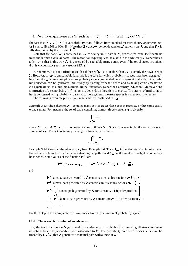
Example 3.13 The collectionFE contains many sets of traces that occur in practice, or that come easilyto one’s mind. For instance, the set of paths containing at most three elementsa is given by[�2X C�;whereX = f� 2 Path�(A) j � contains at most threea’sg. SinceX is countable, the set above is anelement ofFE. The set containing the single infinite path� equals\�v�;�6=�C�:Example 3.14 Consider the adversaryE2 from Example 3.6. ThenE2 is just the sets of all infinite paths.The setC� contains the infinite paths extending the path� andFE2 is the smallest�–algebra containingthose cones. Some values of the functionPE2 arePE2 [Ch" snd(0) �1100 1i℄ = QE2(h"snd(0)�11001i) = 14 � 99100 :and PE2 [a max. path generated byE contains at most three actionssnd(0)℄ �PE2 [a max. path generated byE contains finitely many actionssnd(0)℄ =PE2 "[i a max. path generated byE contains nosnd(0) after positioni# =limi!1PE2 [a max. path generated byE contains nosnd(0) after positioni℄ =limi!1 0 = 0:The third step in this computation follows easily from the definition of probability space.

3.2.4 The trace distribution of an adversary

Now, the trace distributionH generated by an adversaryE is obtained by removing all states and inter-nal actions from the probability space associated toE. The probability on a set of tracesX is now theprobabilityPH [X ℄ thatE generates a maximal path with a trace inX .

15

Definition 3.15 The trace distributionH of an adversaryE, denoted bytrdistr(E ), is the probabilityspace given by

1. H = A tA� [A tA1,

2. FH is the smallest�-field that contains the setsfC� j � 2 A tA�g, whereC� = f�0 2 H j �v�0g,3. PH is given byPH [X ℄ = PE [f� 2 E j tra e(�) 2 Xg℄ for all X 2 FH .

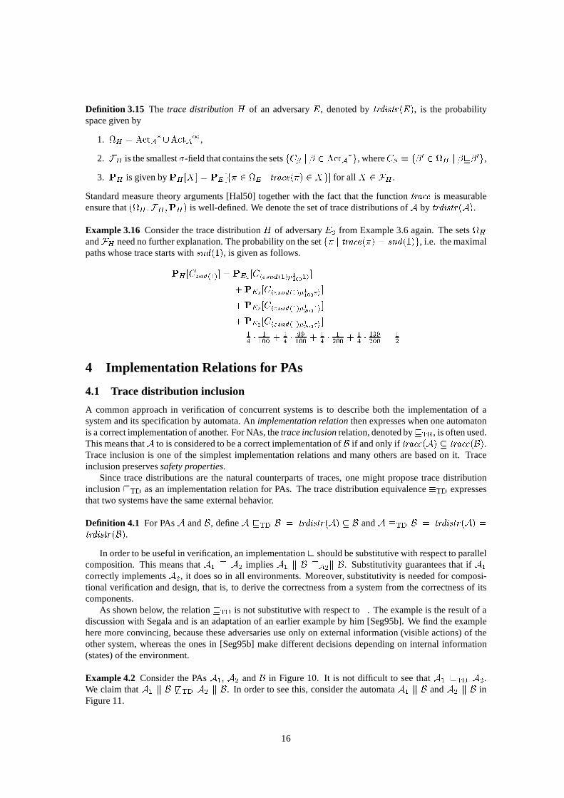
Standard measure theory arguments [Hal50] together with the fact that the functiontra e is measurableensure that(H ;FH ;PH ) is well-defined. We denote the set of trace distributions ofA by trdistr(A).Example 3.16 Consider the trace distributionH of adversaryE2 from Example 3.6 again. The setsHandFH need no further explanation. The probability on the setf� j tra e(�) = snd(1)g, i.e. the maximalpaths whose trace starts withsnd(1), is given as follows.PH [Csnd(1)℄ = PE2 [Ch"snd(1)�11001i℄+PE2 [Ch"snd(1)�1100"i℄+PE2 [Ch"snd(1)�12001i℄+PE2 [Ch"snd(1)�1200"i℄= 14 � 1100 + 14 � 99100 + 14 � 1200 + 14 � 199200 = 124 Implementation Relations for PAs

4.1 Trace distribution inclusion

A common approach in verification of concurrent systems is todescribe both the implementation of asystem and its specification by automata. Animplementation relationthen expresses when one automatonis a correct implementation of another. For NAs, thetrace inclusionrelation, denoted byvTR, is often used.This means thatA to is considered to be a correct implementation ofB if and only if tra e(A) � tra e(B).Trace inclusion is one of the simplest implementation relations and many others are based on it. Traceinclusion preservessafety properties.

Since trace distributions are the natural counterparts of traces, one might propose trace distributioninclusionvTD as an implementation relation for PAs. The trace distribution equivalence�TD expressesthat two systems have the same external behavior.

Definition 4.1 For PAsA andB, defineA vTD B = trdistr(A) � B andA �TD B = trdistr(A) =trdistr(B).In order to be useful in verification, an implementationv should be substitutive with respect to parallel

composition. This means thatA1 v A2 impliesA1 k B vA2k B. Substitutivity guarantees that ifA1correctly implementsA2, it does so in all environments. Moreover, substitutivity is needed for composi-tional verification and design, that is, to derive the correctness from a system from the correctness of itscomponents.

As shown below, the relationvTD is not substitutive with respect tok. The example is the result of adiscussion with Segala and is an adaptation of an earlier example by him [Seg95b]. We find the examplehere more convincing, because these adversaries use only onexternal information (visible actions) of theother system, whereas the ones in [Seg95b] make different decisions depending on internal information(states) of the environment.

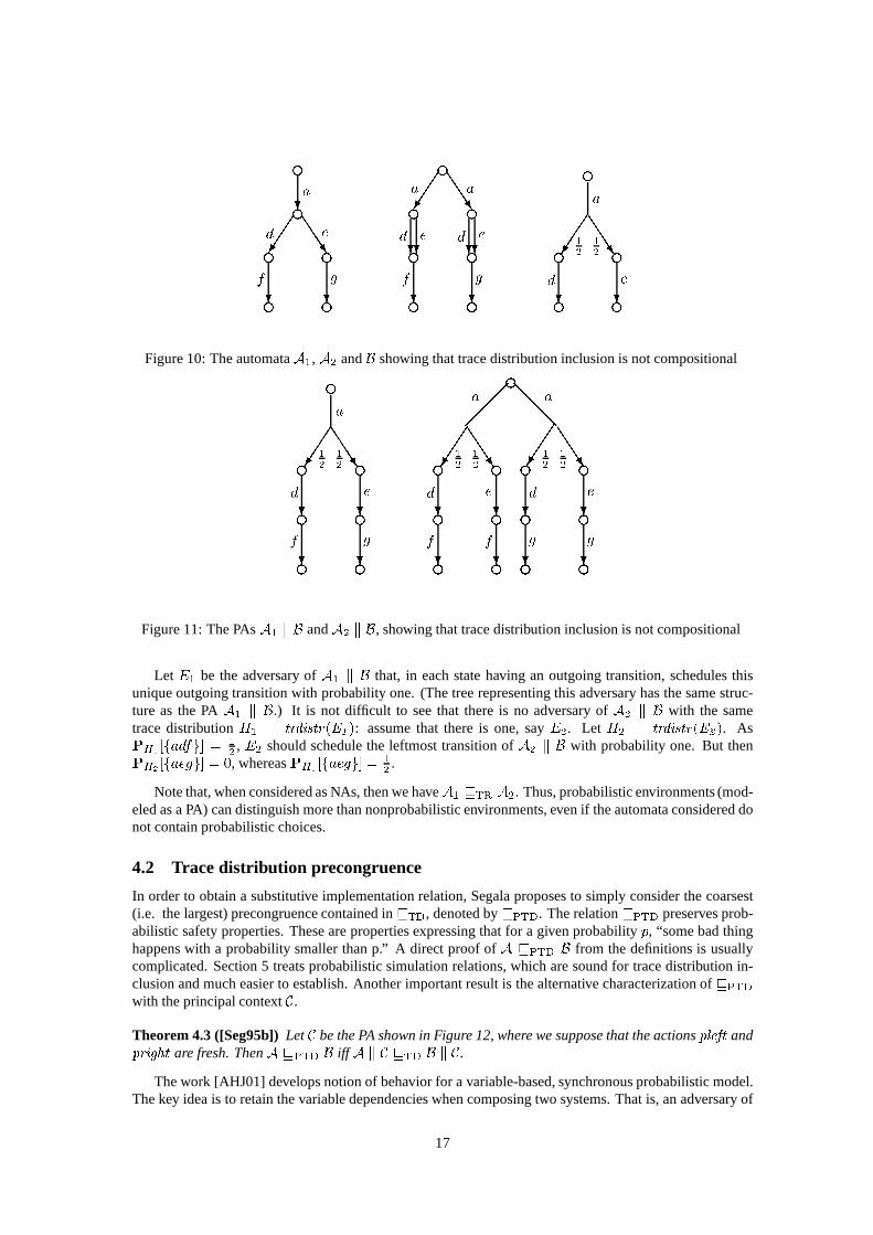
Example 4.2 Consider the PAsA1, A2 andB in Figure 10. It is not difficult to see thatA1 vTD A2.We claim thatA1 k B 6vTD A2 k B. In order to see this, consider the automataA1 k B andA2 k B inFigure 11.

16

e?ae� JJJede e? ?f geee� JJJaae e?? ??d e ede e? ?f gee e ee ee � JJJ? ?12 12d ea

Figure 10: The automataA1,A2 andB showing that trace distribution inclusion is not compositionale� JJJa12 12 ee? ?d eee? ?f geee��� ���� JJJa12 12 ee? ?d eee? ?g ge e

� JJJa12 12 ee? ?d e ee? ?f f eeFigure 11: The PAsA1 k B andA2 k B, showing that trace distribution inclusion is not compositional

Let E1 be the adversary ofA1 k B that, in each state having an outgoing transition, schedules thisunique outgoing transition with probability one. (The treerepresenting this adversary has the same struc-ture as the PAA1 k B.) It is not difficult to see that there is no adversary ofA2 k B with the sametrace distributionH1 = trdistr(E1 ): assume that there is one, sayE2. Let H2 = trdistr(E2 ). AsPH1 [fadfg℄ = 12 , E2 should schedule the leftmost transition ofA2 k B with probability one. But thenPH2 [faegg℄ = 0, whereasPH1 [faegg℄ = 12 .

Note that, when considered as NAs, then we haveA1 vTR A2. Thus, probabilistic environments (mod-eled as a PA) can distinguish more than nonprobabilistic environments, even if the automata considered donot contain probabilistic choices.

4.2 Trace distribution precongruence

In order to obtain a substitutive implementation relation,Segala proposes to simply consider the coarsest(i.e. the largest) precongruence contained invTD, denoted byvPTD. The relationvPTD preserves prob-abilistic safety properties. These are properties expressing that for a given probabilityp, “some bad thinghappens with a probability smaller than p.” A direct proof ofA vPTD B from the definitions is usuallycomplicated. Section 5 treats probabilistic simulation relations, which are sound for trace distribution in-clusion and much easier to establish. Another important result is the alternative characterization ofvPTDwith the principal contextC.

Theorem 4.3 ([Seg95b])LetC be the PA shown in Figure 12, where we suppose that the actionspleft andpright are fresh. ThenA vPTD B iff A k C vTD B k C.

The work [AHJ01] develops notion of behavior for a variable-based, synchronous probabilistic model.The key idea is to retain the variable dependencies when composing two systems. That is, an adversary of

17

e ee��� ���R'-pleft $� pright12 12��� �-pleft ���� pright

Figure 12: Principal context

the composed system is a product of two adversaries for the component systems and one for the environ-ment.

Remark 4.4 (Trace distributions versus traces)Recall from Remark 2.8 that each NA can be interpretedas a PA by simply considering the target state of a transitionas a Dirac distribution. Then the question ariseswhether two trace equivalent NAs are also trace distribution equivalent. Surprisingly, this is not the case. In[Sto02], it is shown that trace equivalence and trace distribution equivalence coincide for finitely branchingNAs, that is, for NAs in which the number of outgoing transitions in a state is finite. It is conjectured thatthis also holds for countably branching NAs. However, for uncountably branching NAs, the result fails.

5 Probabilistic Simulation and Bisimulation

Simulation and bisimulation relations are a useful tool forsystem analysis. Both relations are sound fortrace-based relations, while they are much easier to establish. Furthermore, bisimulation relations allowone to reduce a system to equivalent but smaller system, which is obtained by replacing each state in asystem by its bisimulation equivalence class.

(Bi-)simulation relations have been developed for many different systems, including timed and hybridsystems. This section discusses weak and strong probabilistic (bi-)simulations.

Recall that in the non-probabilistic case a bisimulation isan equivalenceR on the state spaceS suchthat (s; s0) 2 R ands a�! t imply that there is a transitions0 a�! t0 and(s0; t0) 2 R. Since the target ofa transition a PA is a probability distribution rather than asingle state, a probabilistic bisimulation has tocompare probability distributions� and�0 when matching transitionss a�! � ands0 a�! �0 in related statessands0. The idea is as follows. Since bisimilar states are interchangeable, it does not matter which elementwithin the same bisimulation equivalence class is reached.Hence, a bisimulation relation compares theprobability to reach the equivalence classes, rather than the probability to reach a single element. Thus, welift an equivalence relationR onS to a relation onDistr(S) in as follows.

Definition 5.1 Let X be a set and letR an equivalence relation onX . Then the lifting ofR to Distr(S),denoted by�R, is defined by � �R �0 = 8C[�[C℄ = �0[C℄℄:whereC ranges over the setX=R of equivalence classes moduloR.

Definition 5.2 (Strong bisimulation) An equivalence relationR � S�S is astrong simulationiff for all(s; s0) 2 Rif s a�!� then there is a transitions0 a�!�0 with � �R �0.

The statess ands0 arestrongly bisimilar, notations �sbis s0, if there exists a bisimulationR containing(s; s0).18

z z zy x1 x2s a, �

i i ii i ii

z zy0 x0s0a, �0ii iii

b b ? ? ? ? ?���� ���R? ���� AAAU12 18 38 12 12 v vy0 x0s0a, �0ii iii

b ? ?���� AAAU13 23 s0t0 u0v0 v0 v0

ii ii i i

a, �0b ?���� AAAU ��� ���R1212

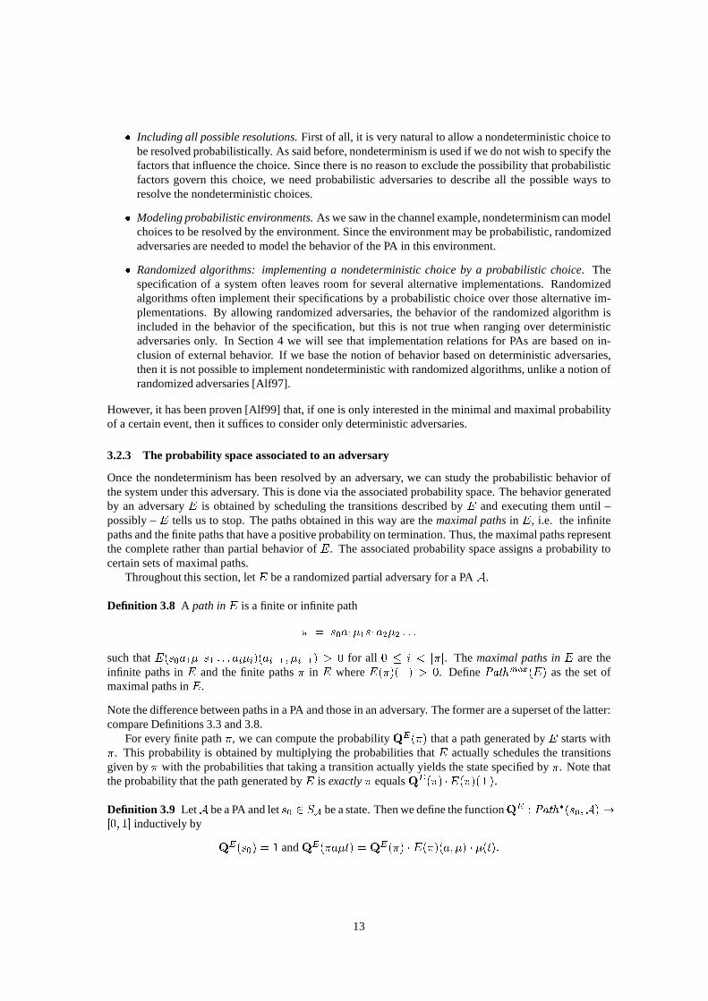
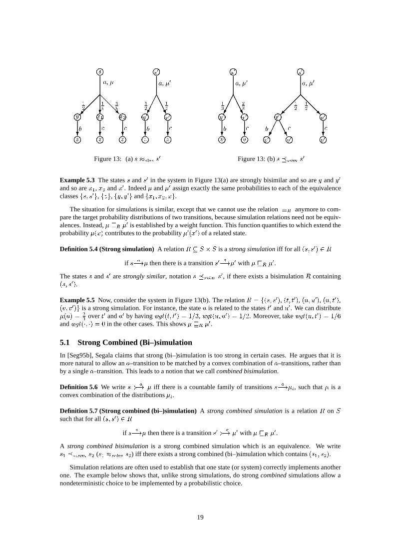
Figure 13: (a)s �sbis s0 Figure 13: (b)s �ssim s0Example 5.3 The statess ands0 in the system in Figure 13(a) are strongly bisimilar and so are y andy0and so arex1, x2 andx0. Indeed� and�0 assign exactly the same probabilities to each of the equivalenceclassesfs; s0g, fzg, fy; y0g andfx1; x2; xg.

The situation for simulations is similar, except that we cannot use the relation�R anymore to com-pare the target probability distributions of two transitions, because simulation relations need not be equiv-alences. Instead,� vR �0 is established by a weight function. This function quantifies to which extend theprobability�(x) contributes to the probability�0(x0) of a related state.

Definition 5.4 (Strong simulation) A relationR � S � S is astrong simulationiff for all (s; s0) 2 Rif s a�!� then there is a transitions0 a�!�0 with � vR �0.

The statess ands0 arestrongly similar, notations �ssim s0, if there exists a bisimulationR containing(s; s0).Example 5.5 Now, consider the system in Figure 13(b). The relationR = f(s; s0), (t; t0), (u; u0), (u; t0),(v; v0)g is a strong simulation. For instance, the stateu is related to the statest0 andu0. We can distribute�(u) = 23 overt0 andu0 by havingwgt(t; t0) = 1=3, wgt(u; u0) = 1=2. Moreover, takewgt(u; t0) = 1=6andwgt(�; �) = 0 in the other cases. This shows� vR �0.5.1 Strong Combined (Bi–)simulation

In [Seg95b], Segala claims that strong (bi–)simulation is too strong in certain cases. He argues that it ismore natural to allow ana–transition to be matched by a convex combination ofa–transitions, rather thanby a singlea–transition. This leads to a notion that we callcombined bisimulation.

Definition 5.6 We write s �a! � iff there is a countable family of transitionss a�!�i, such that� is aconvex combination of the distributions�i.Definition 5.7 (Strong combined (bi–)simulation) A strong combined simulationis a relationR on Ssuch that for all(s; s0) 2 R

if s a�!� then there is a transitions0 �a! �0 with � vR �0.A strong combined bisimulationis a strong combined simulation which is an equivalence. We writes1 �s sim s2 (s1 �s bis s2) iff there exists a strong combined (bi–)simulation which contains(s1; s2).

Simulation relations are often used to establish that one state (or system) correctly implements anotherone. The example below shows that, unlike strong simulations, do strongcombinedsimulations allow anondeterministic choice to be implemented by a probabilistic choice.

19

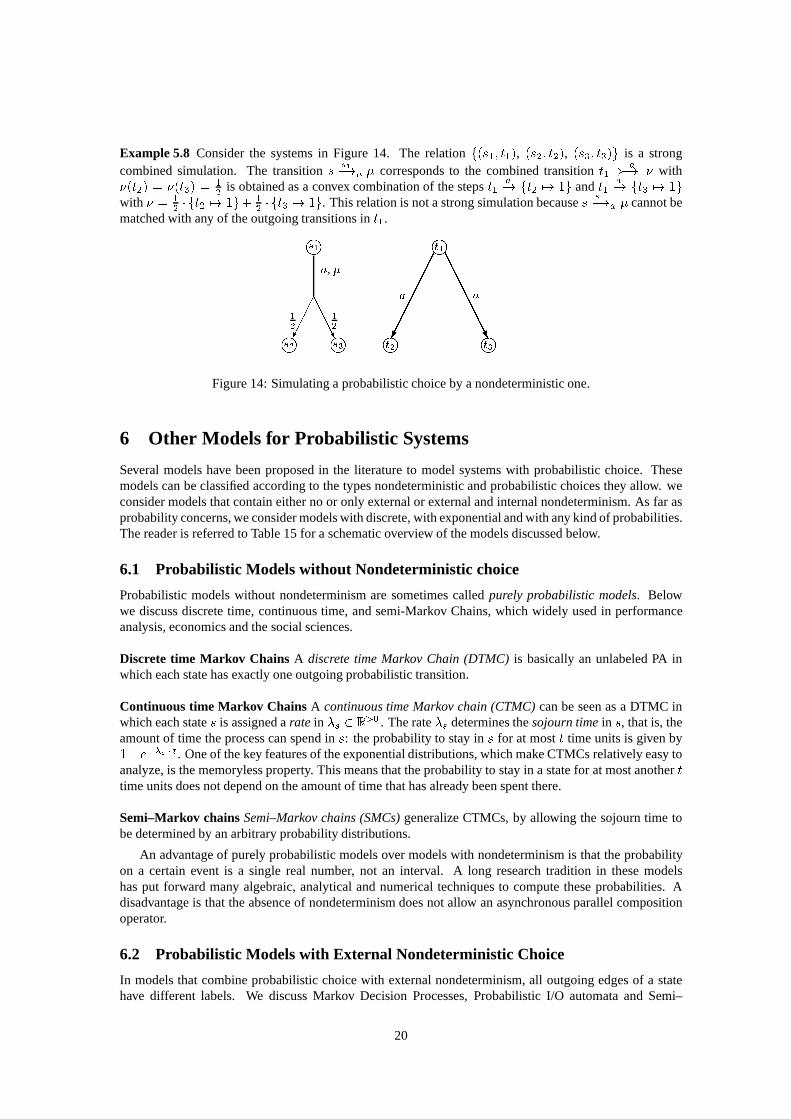
Example 5.8 Consider the systems in Figure 14. The relationf(s1; t1), (s2; t2), (s3; t3)g is a strongcombined simulation. The transitions s1�!a � corresponds to the combined transitiont1 �a! � with�(t2) = �(t3) = 12 is obtained as a convex combination of the stepst1 a�! ft2 7! 1g andt1 a�! ft3 7! 1gwith � = 12 � ft2 7! 1g+ 12 � ft3 7! 1g. This relation is not a strong simulation becauses s1�!a � cannot bematched with any of the outgoing transitions int1.s1

s2 s3a, �j jj����� AAAAU12 12 t1

t2 t3a ajj j�������� AAAAAAAU

Figure 14: Simulating a probabilistic choice by a nondeterministic one.

6 Other Models for Probabilistic Systems

Several models have been proposed in the literature to modelsystems with probabilistic choice. Thesemodels can be classified according to the types nondeterministic and probabilistic choices they allow. weconsider models that contain either no or only external or external and internal nondeterminism. As far asprobability concerns, we consider models with discrete, with exponential and with any kind of probabilities.The reader is referred to Table 15 for a schematic overview ofthe models discussed below.

6.1 Probabilistic Models without Nondeterministic choice

Probabilistic models without nondeterminism are sometimes calledpurely probabilistic models. Belowwe discuss discrete time, continuous time, and semi-MarkovChains, which widely used in performanceanalysis, economics and the social sciences.

Discrete time Markov Chains A discrete time Markov Chain (DTMC)is basically an unlabeled PA inwhich each state has exactly one outgoing probabilistic transition.

Continuous time Markov Chains A continuous time Markov chain (CTMC)can be seen as a DTMC inwhich each states is assigned arate in �s 2 R>0 . The rate�s determines thesojourn timein s, that is, theamount of time the process can spend ins: the probability to stay ins for at mostt time units is given by1�e��s � t. One of the key features of the exponential distributions, which make CTMCs relatively easy toanalyze, is the memoryless property. This means that the probability to stay in a state for at most anotherttime units does not depend on the amount of time that has already been spent there.

Semi–Markov chainsSemi–Markov chains (SMCs)generalize CTMCs, by allowing the sojourn time tobe determined by an arbitrary probability distributions.

An advantage of purely probabilistic models over models with nondeterminism is that the probabilityon a certain event is a single real number, not an interval. A long research tradition in these modelshas put forward many algebraic, analytical and numerical techniques to compute these probabilities. Adisadvantage is that the absence of nondeterminism does notallow an asynchronous parallel compositionoperator.

6.2 Probabilistic Models with External Nondeterministic Choice

In models that combine probabilistic choice with external nondeterminism, all outgoing edges of a statehave different labels. We discuss Markov Decision Processes, Probabilistic I/O automata and Semi–

20

Markov decision processes. The advantage of these models isthat an asynchronous parallel compositionoperator can be defined, allowing a large system to be split upby several smaller components. Furthermore,when we put the system in an purely probabilistic environment (such that each system transition synchro-nizes with an environment transition), the whole system becomes purely probabilistic and the analysistechniques for these systems can be used.

Markov Decision ProcessesA Markov Decision Process (MDP)is a PA without internal actions in whicheach state contains at most one outgoing transition labeledwith a.

Probabilistic I/O automata Probabilistic I/O automata (PIOAs) [WSS97] combine external nondetermin-ism with exponential probability distributions. The memoryless property of these distributions allows asmooth definition of a parallel composition operator, as faras independent transitions are concerned. Forsynchronizing transitions, the situation is more difficult. Various solutions have been proposed. We findthe solution adopted in PIOAs one of the cleanest. This modelpartitions the visible actions into input andoutput actions. Output and internal actions are governed byrates. This means that they can only been takenwhen the sojourn time has expired. Furthermore, the choice between the various output or internal actionis purely probabilistic. Input actions, on the other hand, are always enabled and can be taken before thesojourn time has expired.

Semi–Markov decision processesPuterman [Put94] discusses Semi–Markov decision processes (SMDPs),which are basically Semi–Markov chains with external nondeterministic choice.

6.3 Probabilistic Models with Full Nondeterminism

Probabilistic automata We have already seen that probabilistic automata and variants thereof combinenondeterministic and discrete probabilistic choice. Several process algebras, such as ACP [And99b, And99a],the probabilistic�–calculus and the probabilistic process algebra defined in [Han94], allow one to describesuch models algebraically.

Interactive Markov chains Interactive Markov Chains (IMCs) [Her99] combine exponential distributionswith full nondeterminism. The definition of a parallel composition operator poses the same problems aswhen one combines exponential distributions with externalnondeterminism. IMCs propose an elegantsolution by distinguishing between interactive transitions and Markovian transitions. Theinteractive tran-sitionsallow one to specify external and internal nondeterministic choices and they synchronize (exceptfor the � transition) with their environment. TheMarkovian transitionsspecify the rate with which thetransition is taken, similarly to CTMCs.

SPADESFull nondeterminism and arbitrary probability distributions are combined in the process algebraSPADES (also written ) and its underlying semantic modelstochastic automata(SAs). The sojourntime in a state of an SA is specified via clocks, which can have arbitrary probability distributions. Moreprecisely, each transition is decorated with a (possibly empty) set of clocks� and can only be taken when allclocks in� have expired. In that case all clocks in� are assigned new values according to their probabilitydistributions. Stochastic automata in their turn have a semantics in terms of stochastic transition systems.These are transition systems in which the target of a transition can be an arbitrary probability space.

7 Summary

The probabilistic automaton model discussed in this paper combines discrete probabilistic choice and non-deterministic choice in an orthogonal way. This allows us todefine an asynchronous parallel compositionoperator and makes the model suitable for reasoning about randomized distributed algorithms, probabilisticcommunication protocols and systems with failing components. PAs subsume nonprobabilistic transitionsystems, Markov decision processes and Markov chains. Nondeterministic timing can be naturally incor-

21

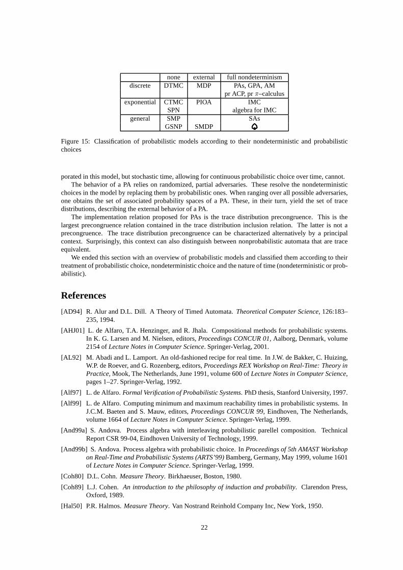
none external full nondeterminismdiscrete DTMC MDP PAs, GPA, AM

pr ACP, pr�–calculusexponential CTMC PIOA IMC

SPN algebra for IMCgeneral SMP SAs

GSNP SMDP

Figure 15: Classification of probabilistic models according to their nondeterministic and probabilisticchoices

porated in this model, but stochastic time, allowing for continuous probabilistic choice over time, cannot.The behavior of a PA relies on randomized, partial adversaries. These resolve the nondeterministic

choices in the model by replacing them by probabilistic ones. When ranging over all possible adversaries,one obtains the set of associated probability spaces of a PA.These, in their turn, yield the set of tracedistributions, describing the external behavior of a PA.

The implementation relation proposed for PAs is the trace distribution precongruence. This is thelargest precongruence relation contained in the trace distribution inclusion relation. The latter is not aprecongruence. The trace distribution precongruence can be characterized alternatively by a principalcontext. Surprisingly, this context can also distinguish between nonprobabilistic automata that are traceequivalent.

We ended this section with an overview of probabilistic models and classified them according to theirtreatment of probabilistic choice, nondeterministic choice and the nature of time (nondeterministic or prob-abilistic).

References

[AD94] R. Alur and D.L. Dill. A Theory of Timed Automata.Theoretical Computer Science, 126:183–235, 1994.

[AHJ01] L. de Alfaro, T.A. Henzinger, and R. Jhala. Compositional methods for probabilistic systems.In K. G. Larsen and M. Nielsen, editors,Proceedings CONCUR 01,Aalborg, Denmark, volume2154 ofLecture Notes in Computer Science. Springer-Verlag, 2001.

[AL92] M. Abadi and L. Lamport. An old-fashioned recipe for real time. In J.W. de Bakker, C. Huizing,W.P. de Roever, and G. Rozenberg, editors,Proceedings REX Workshop on Real-Time: Theory inPractice,Mook, The Netherlands, June 1991, volume 600 ofLecture Notes in Computer Science,pages 1–27. Springer-Verlag, 1992.

[Alf97] L. de Alfaro. Formal Verification of Probabilistic Systems. PhD thesis, Stanford University, 1997.

[Alf99] L. de Alfaro. Computing minimum and maximum reachability times in probabilistic systems. InJ.C.M. Baeten and S. Mauw, editors,Proceedings CONCUR 99,Eindhoven, The Netherlands,volume 1664 ofLecture Notes in Computer Science. Springer-Verlag, 1999.

[And99a] S. Andova. Process algebra with interleaving probabilistic parellel composition. TechnicalReport CSR 99-04, Eindhoven University of Technology, 1999.

[And99b] S. Andova. Process algebra with probabilistic choice. InProceedings of 5th AMAST Workshopon Real-Time and Probabilistic Systems (ARTS’99)Bamberg, Germany, May 1999, volume 1601of Lecture Notes in Computer Science. Springer-Verlag, 1999.

[Coh80] D.L. Cohn.Measure Theory. Birkhaeuser, Boston, 1980.

[Coh89] L.J. Cohen.An introduction to the philosophy of induction and probability. Clarendon Press,Oxford, 1989.

[Hal50] P.R. Halmos.Measure Theory. Van Nostrand Reinhold Company Inc, New York, 1950.

22

[Han94] H.A. Hansson.Time and Probability in Formal Design of Distributed Systems, volume 1 ofReal-Time Safety Critical Systems. Elsevier, 1994.

[Her99] H.H. Hermanns.Interactive Markov Chains. PhD thesis, University of Erlangen–Nurnberg, July1999. Available viahttp://wwwhome.cs.utwente.nl/˜hermanns .

[HJ94] H. Hansson and B. Jonsson. A logic for reasoning abouttime and reliability.Formal Aspects ofComputing, 6(5):515–535, 1994.

[Hoa85] C.A.R. Hoare.Communicating Sequential Processes. Prentice-Hall International, EnglewoodCliffs, 1985.

[HP00] O.M. Herescu and C. Palamidessi. Probabilistic asynchronous�-calculus. In J. Tiuryn, editor,Proceedings of 3rd International Conference on Foundations of Science and Computation Struc-tures (FOSSACS),Berlin, Germany, March 2000, volume 1784 ofLecture Notes in ComputerScience, pages 1–16. Springer-Verlag, 2000.

[IEE96] IEEE Computer Society. IEEE Standard for a High Performance Serial Bus. Std 1394-1995,August 1996.

[KNSS01] M. Z. Kwiatkowska, G. Norman, R. Segala, and J. Sproston. Automatic verification of real-timesystems with discrete probability distributions.Theoretical Computer Science, 268, 2001.

[LR81] D. Lehmann and M. Rabin. On the advantage of free choice: a symmetric and fully distributedsolution to the dining philosophers problem. InProceedings of the 8th ACM Symposium onPrinciples of Programming Languages, pages 133–138, 1981.

[LS91] K.G. Larsen and A. Skou. Bisimulation through probabilistic testing. Information and Computa-tion, 94:1–28, 1991.

[LT89] N.A. Lynch and M.R. Tuttle. An introduction to input/output automata.CWI Quarterly, 2(3):219–246, September 1989.

[LV96] N.A. Lynch and F.W. Vaandrager. Forward and backwardsimulations, II: Timing-based systems.Information and Computation, 128(1):1–25, July 1996.

[Put94] M. Puterman.Markov Decision Processes. John Wiley and Sons, 1994.

[Seg95a] R. Segala. Compositional trace–based semantics for probabilistic automata. InProc. CON-CUR’95, volume 962 ofLecture Notes in Computer Science, pages 234–248, 1995.

[Seg95b] R. Segala.Modeling and Verification of Randomized Distributed Real-Time Systems. PhD thesis,Department of Electrical Engineering and Computer Science, Massachusetts Institute of Techno-logy, June 1995. Available as Technical Report MIT/LCS/TR-676.

[SL95] R. Segala and N.A. Lynch. Probabilistic simulationsfor probabilistic processes.Nordic Journalof Computing, 2(2):250–273, 1995.

[Sto02] Marielle Stoelinga. Alea jacta est: verification of probabilistic, real-time and parametricsystems. PhD thesis, University of Nijmegen, the Netherlands, April 2002. Available viahttp://www.soe.ucsc.edu/˜marielle .

[Tan81] A.S. Tanenbaum.Computer networks. Prentice-Hall International, Englewood Cliffs, 1981.

[WSS97] S.-H. Wu, S.A. Smolka, and E. Stark. Composition andand behaviors of probabilistic I/Oautomata.Theoretical Computer Science, 1-2:1–38, 1997.

[Yi90] Wang Yi. Real-time behaviour of asynchronous agents. In J.C.M. Baeten and J.W. Klop, editors,Proceedings CONCUR 90,Amsterdam, volume 458 ofLecture Notes in Computer Science, pages502–520. Springer-Verlag, 1990.

23