An Introduction to Random Field Theory

Matthew Brett∗, Will Penny† and Stefan Kiebel†∗ MRC Cognition and Brain Sciences Unit, Cambridge UK;

† Functional Imaging Laboratory, Institute of Neurology, London, UK.

March 4, 2003

1 Introduction

This chapter is an introduction to the multiple comparison problem in func-tional imaging, and the way it can be solved using Random field theory(RFT).

In a standard functional imaging analysis, we fit a statistical model tothe data, to give us model parameters. We then use the model parametersto look for an effect we are interested in, such as the difference between atask and baseline. To do this, we usually calculate a statistic for each brainvoxel that tests for the effect of interest in that voxel. The result is a largevolume of statistic values.

We now need to decide if this volume shows any evidence of the effect.To do this, we have to take into account that there are many thousands ofvoxels and therefore many thousands of statistic values. This is the multiplecomparison problem in functional imaging. Random field theory is a recentbranch of mathematics that can be used to solve this problem.

To explain the use of RFT, we will first go back to the basics of hypothesistesting in statistics. We describe the multiple comparison problem and theusual solution, which is the Bonferroni correction. We explain why spatialcorrelation in imaging data causes problems for the Bonferroni correction andintroduce RFT as a solution. Finally, we discuss the assumptions underlyingRFT and the problems that arise when these assumptions do not hold. Wehope this chapter will be accessible to those with no specific expertise inmathematics or statistics. Those more interested in mathematical detailsand recent developments are referred to Chapter 15.

1

1.1 Rejecting the null hypothesis

When we calculate a statistic, we often want to decide whether the statisticrepresents convincing evidence of the effect we are interested in. Usually wetest the statistic against the null hypothesis, which is the hypothesis thatthere is no effect. If the statistic is not compatible with the null hypothesis,we may conclude that there is an effect. To test against the null hypothe-sis, we can compare our statistic value to a null distribution, which is thedistribution of statistic values we would expect if there is no effect. Usingthe null distribution, we can estimate how likely it is that our statistic couldhave come about by chance. We may find that the result we found has a 5%chance of resulting from a null distribution. We therefore decide to reject thenull hypothesis, and accept the alternative hypothesis that there is an effect.In rejecting the null hypothesis, we must accept a 5% chance that the resulthas in fact arisen when there is in fact no effect, i.e. the null hypothesis istrue. 5% is our expected type I error rate, or the chance that we take thatwe are wrong when we reject the null hypothesis.

For example, when we do a single t test, we compare the t value we havefound to the null distribution for the t statistic. Let us say we have founda t value of 2.42, and have 40 degrees of freedom. The null distribution of tstatistics with 40 degrees of freedom tells us that the probability of observinga value greater than or equal to 2.42, if there is no effect, is only 0.01. In ourcase, we can reject the null hypothesis with a 1% risk of type I error.

The situation is more complicated in functional imaging because we havemany voxels and therefore many statistic values. If we do not know where inthe brain our effect will occur, our hypothesis refers to the whole volume ofstatistics in the brain. Evidence against the null hypothesis would be thatthe whole observed volume of values is unlikely to have arisen from a nulldistribution. The question we are asking is now a question about the volume,or family of voxel statistics, and the risk of error that we are prepared toaccept is the Family–Wise Error rate (FWE) — which is the likelihood thatthis family of voxel values could have arisen by chance.

We can test a family-wise null hypothesis in a variety of ways, but oneuseful method is to look for any statistic values that are larger than we wouldexpect, if they all had come from a null distribution. The method requiresthat we find a threshold to apply to every statistic value, so that any valuesabove the threshold are unlikely to have arisen by chance. This is oftenreferred to as “height thresholding”, and it has the advantage that if we findvoxels above threshold, we can conclude that there is an effect at these voxellocations — i.e. the test has localizing power. Alternative procedures basedon cluster- and set-level inferences are discussed in section 4.

2

A height threshold that can control family-wise error must take into ac-count the number of tests. We saw above that a single t statistic value froma null distribution with 40 degrees of freedom has a 1% probability of beinggreater than 2.42. Now imagine our experiment has generated 1000 t valueswith 40 degrees of freedom. If we look at any single statistic, then by chanceit will have a 1% probability of being greater than 2.42. This means thatwe would expect 10 t values in our sample of 1000 to be greater than 2.42.So, if we see one or more t values above 2.42 in this family of tests, this isnot good evidence against the family-wise null hypothesis, which is that allthese values have been drawn from a null distribution. We need to find anew threshold, such that, in a family of 1000 t statistic values, there is a 1%probability of there being one or more t values above that threshold. TheBonferroni correction is a simple method of setting this threshold.

2 The Bonferroni correction

The Bonferroni correction is based on simple probability rules. Imagine wehave taken our t values and used the null t distribution to convert themto probability values. We then apply a probability threshold α to each ofour n probability values; in our previous example α was 0.01, and n was1000. If all the test values are drawn from a null distribution, then each ofour n probability values has a probability α of being greater than threshold.The probability of all the tests being less than α is therefore (1− α)n. Thefamily-wise error rate (P FWE) is the probability that one or more values willbe greater than α, which is simply:

P FWE = 1− (1− α)n (1)

Because α is small this can be approximated by the simpler expression:

P FWE ≤ nα (2)

Using equation 2, we can find a single-voxel probability threshold α thatwill give us our required family-wise error rate, P FWE, such that we have aP FWE probability of seeing any voxel above threshold in all of the n values.We simply solve equation 2 for α:

α = P FWE/n (3)

3

If we have a brain volume of 100,000 t statistics, all with 40 degreesof freedom, and we want a FWE rate of 0.05, then the required probabil-ity threshold for a single voxel, using the Bonferroni correction, would be0.05/100, 000 = 0.0000005. The corresponding t statistic is 5.77. If anyvoxel t statistic is above 5.77, then we can conclude that a voxel statisticof this magnitude has only a 5% chance of arising anywhere in a volume of100,000 t statistics drawn from the null distribution.

The Bonferroni procedure gives a corrected p value; in the case above,the uncorrected p value for a voxel with a t statistic of 5.77 was 0.0000005;the p value corrected for the number of comparisons is 0.05.

The Bonferroni correction is used for calculating FWE rates for somefunctional imaging analyses. However, in many cases, the Bonferroni cor-rection is too conservative because most functional imaging data have somedegree of spatial correlation - i.e. there is correlation between neighbour-ing statistic values. In this case, there are fewer independent values in thestatistic volume than there are voxels.

2.1 Spatial correlation

Some degree of spatial correlation is almost universally present in functionalimaging data. In general, data from any one voxel in the functional image willtend to be similar to data from nearby voxels, even after the modelled effectshave been removed. Thus the errors from the statistical model will tend tobe correlated for nearby voxels. The reasons for this include factors inherentin collecting the image, physiological signal that has not been modeled, andspatial preprocessing applied to the data before statistical analysis.

For PET data, much more than for FMRI, nearby voxels are relatedbecause of the way that the scanner collects and reconstructs the image.Thus, data that does in fact arise from a single voxel location in the brain willalso cause some degree of signal change in neighbouring voxels in the resultingimage. The extent to which this occurs is a measure of the performance ofthe PET scanner, and is referred to as the point spread function.

Spatial preprocessing of functional data introduces spatial correlation.Typically, we will realign images for an individual subject to correct for mo-tion during the scanning session (see Chapter 2), and may also spatiallynormalize a subject’s brain to a template to compare data between subjects(see Chapter 3). These transformations will require the creation of new re-sampled images, which have voxel centres that are very unlikely to be thesame as those in the original images. The resampling requires that we esti-mate the signal for these new voxel locations from the values in the originalimage, and typical resampling methods require some degree of averaging of

4

neighbouring voxels to derive the new voxel value (see Chapter 2).It is very common to smooth the functional images before statistical anal-

ysis. A proportion of the noise in functional images is independent from voxelto voxel, whereas the signal of interest usually extends over several voxels.This is due both to the possibly distributed nature of neuronal sources andthe spatially extended nature of the haemodynamic response (see Chapter11). According to the matched filter theorem smoothing will therefore im-prove the signal to noise ratio. For multiple subject analyses, smoothingmay also be useful for blurring the residual differences in location betweencorresponding areas of functional activation. Smoothing involves averagingover voxels, which will by definition increase spatial correlation.

2.2 The Bonferroni correction and independent obser-vations

Spatial correlation means that there are fewer independent observations inthe data than there are voxels. This means that the Bonferroni correctionwill be too conservative because the family–wise probability from equation1 relies on the individual probability values being independent, so that wecan use multiplication to calculate the probability of combined events. Forequation 1, we used multiplication to calculate the probability that all testswill be below threshold with (1 − α)n. Thus the n in the equation must bethe number of independent observations. If we have n voxels in our data,but there are only ni independent observations, then equation 1 becomesP FWE = 1− (1− α)ni , and the corresponding α from equation 3 is given byα = P FWE/ni. This is best illustrated by example.

Let us take a single image slice, of 100 by 100 voxels, with a t statisticvalue for each voxel. For the sake of simplicity, let the t statistics have veryhigh degrees of freedom, so that we can consider the t statistic values asbeing from the normal distribution - i.e. that they are Z scores. We cansimulate this slice from a null distribution by filling the voxel values withindependent random numbers from the normal distribution, which results inan image such as that in figure 1.

If this image had come from the analysis of real data, we might want totest if any of the numbers in the image are more positive than is likely bychance. The values are independent, so the Bonferroni correction will give anaccurate threshold. There are 10,000 Z scores, so the Bonferroni threshold,α, for a FWE rate of 0.05, is 0.05/10000 = 0.000005. This corresponds toa Z score of 4.42. Given the null hypothesis (which is true in this case) wewould expect only 5 out of 100 such images to have one or more Z scores

5

more positive than 4.42.The situation changes if we add spatial correlation. Let us perform the

following procedure on the image: break up the image into squares of 10 by10 pixels; for each square, calculate the mean of the 100 values contained;replace the 100 random numbers in the square by the mean value1. Theimage that results is shown in figure 2.

We still have 10000 numbers in our image, but there are only 10 by 10 =100 numbers that are independent. The appropriate Bonferroni correctionis now 0.05 / 100 = 0.0005, which corresponds to a Z score of 3.29. Wewould expect only 5 of 100 of such images to have a square of values greaterthan 3.29 by chance. If we had assumed all the values were independent,then we would have used the correction for 10,000 values, of α = 0.000005.Because we actually have only 100 independent observations, equation 2,with n = 100 and α = 0.000005, tells us that we expect a FWE rate of0.0005, which is one hundred times lower (i.e. more conservative) than therate that we wanted.

2.3 Smoothing and independent observations

In the preceding section we replaced a square of values in the image withtheir mean in order to show the effect of reducing the number of independentobservations. This procedure is a very simple form of smoothing. When wesmooth an image with a smoothing kernel such as a Gaussian, each value inthe image is replaced with a weighted average of itself and its neighbours.Figure 3 shows the image from figure 1 after smoothing with a Gaussiankernel of Full Width at Half Maximum (FWHM) of 10 pixels 2. An FWHMof 10 pixels means that, at five pixels from the centre, the value of the kernelis half its peak value. Smoothing has the effect of blurring the image, andreduces the number of independent observations.

The smoothed image contains spatial correlation, which is typical of theoutput from the analysis of functional imaging data. We now have a problem,because there is no simple way of calculating the number of independent ob-

1Averaging the random numbers will make them tend to zero; to return the image toa variance of 1, we need to multiply the numbers in the image by 10; this is

√n, where n

is the number of values we have averaged.2As for the procedure where we took the mean of the 100 observations in each square,

the smoothed values will no longer have a variance of one, because the averaging involvedin smoothing will make the values tend to zero. As for the square example, we need tomultiply the values in the smoothed image by a scale factor to return the variance toone; the derivation of the scale factor is rather technical, and not relevant to our currentdiscussion.

6

servations in the smoothed data, so we cannot use the Bonferroni correction.This problem can be addressed using random field theory.

3 Random field theory

Random field theory (RFT) is a recent body of mathematics defining theo-retical results for smooth statistical maps. The theory has been versatile indealing with many of the thresholding problems that we encounter in func-tional imaging. Among many other applications, it can be used to solve ourproblem of finding the height threshold for a smooth statistical map whichgives the required family–wise error rate.

The way that RFT solves this problem is by using results that give theexpected Euler characteristic (EC) for a smooth statistical map that hasbeen thresholded. We will discuss the EC in more detail below; for now it isonly necessary to note that the expected EC leads directly to the expectednumber of clusters above a given threshold, and that this in turn gives theheight threshold that we need.

The application of RFT proceeds in stages. First we estimate the smooth-ness (spatial correlation) of our statistical map. Then we use the smoothnessvalues in the appropriate RFT equation, to give the expected EC at differ-ent thresholds. This allows us to calculate the threshold at which we wouldexpect 5% of equivalent statistical maps arising under the null hypothesis tocontain at least one area above threshold.

3.1 Smoothness and resels

Usually we do not know the smoothness of our statistical map. This is so evenif the map resulted from smoothed data, because we usually do not know theextent of spatial correlation in the underlying data before smoothing. If wedo not know the smoothness, it can be calculated using the observed spatialcorrelation in the images. For our example (figure 3), however, we know thesmoothness, because the data were independent before smoothing. In thiscase, the smoothness results entirely from the smoothing we have applied.The smoothness can be expressed as the width of the smoothing kernel, whichwas 10 pixels FWHM in the x and y direction. We can use the FWHM tocalculate the number of resels in the image. “Resel” was a term introducedby Worsley [14], and is a measure of the number of “resolution elements”in the statistical map. This can be thought of as similar to the number ofindependent observations, but it is not the same, as we will see below. Aresel is simply defined as a block of values (in our case, pixels) that is the

7

same size as the FWHM. For the image in figure 3, the FWHMs were 10 by10 pixels, so that a resel is a block of 100 pixels. As there are 10,000 pixelsin our image, there are 100 resels. Note that the number of resels dependsonly on the smoothness (FWHM) and the number of pixels.

3.2 The Euler characteristic

The Euler characteristic is a property of an image after it has been thresh-olded. For our purposes, the EC can be thought of as the number of blobsin an image after thresholding. For example, we can threshold our smoothedimage (figure 3) at Z=2.5; all pixels with Z scores less than 2.5 are set tozero, and the rest are set to one. This results in the image in figure 4.

There are three white blobs in figure 4, corresponding to three areas withZ scores higher than 2.5. The EC of this image is therefore 3. If we increasethe Z score threshold to 2.75, we find that the two central blobs disappear –because the Z scores were less than 2.75 (figure 5).

The area in the upper right of the image remains; the EC of the imagein figure 5 is therefore one. At high thresholds the EC is either one or zero.Hence, the average or expected EC, written E [EC], corresponds (approxi-mately) to the probability of finding an above threshold blob in our statisticimage. That is, the probability of a family wise error is approximately equiv-alent to the expected Euler Characteristic, P FWE ≈ E [EC].

It turns out that if we know the number of resels in our image, it ispossible to calculate E [EC] at any given threshold. For an image of twodimensions E [EC] is given by Worsley [14]. If R is the number of resels, Zt

is the Z score threshold, then:

E [EC] = R(4loge2)(2π)−32 Zte

− 12Z2

t ; (4)

Figure 6 shows E [EC] for an image of 100 resels, for Z score thresholdsbetween zero and five. As the threshold drops from one to zero, E [EC] dropsto zero; this is because the precise definition of the EC is more complex thansimply the number of blobs [9]. This makes a difference at low thresholdsbut is not relevant for our purposes because, as explained above, we areonly interested in the properties of E [EC] at high thresholds ie. when itapproximates P FWE.

Note also that the graph in figure 6 does a reasonable job of predictingthe EC in our image; at a Z threshold of 2.5 it predicted an EC of 1.9, whenwe observed a value of 3; at Z=2.75 it predicted an EC of 1.1, for an observedEC of 1.

8

We can now apply RFT to our smoothed image (figure 3) which has 100resels. For 100 resels, equation 4 gives an E [EC] of 0.049 for a Z threshold of3.8 (c.f. the graph in figure 6). If we have a two dimensional image with 100resels, then the probability of getting one or more blobs where Z is greaterthan 3.8, is 0.049. We can use this for thresholding. Let x be the Z scorethreshold that gives an E [EC] of 0.05. If we threshold our image at x, we canconclude that any blobs that remain have a probability of less than or equalto 0.05 that they have occurred by chance. From equation 4, the threshold,x, depends only on the number of resels in our image.

3.3 Random field thresholds and the Bonferroni cor-rection

The random field correction derived using the EC is not the same as a Bon-ferroni correction for the number of resels. We stated above that the reselcount in an image is not exactly the same as the number of independentobservations. If it was the same, then instead of using RFT, we could usea Bonferroni correction based on the number of resels. However, these twocorrections give different answers. For α = 0.05, the Z threshold accordingto RFT, for our 100 resel image, is Z=3.8. The Bonferroni threshold for 100independent tests, is 0.05/100, which equates to a Z score of 3.3. Althoughthe RFT maths gives us a correction that is similar in principle to a Bonfer-roni correction, it is not the same. If the assumptions of RFT are met (seesection 4) then the RFT threshold is more accurate than the Bonferroni.

3.4 Random fields and functional imaging

Analyses of functional imaging data usually lead to three dimensional statis-tical images. So far we have discussed the application of RFT to an image oftwo dimensions, but the same principles apply in three dimensions. The ECis the number of 3D blobs of Z scores above a certain threshold and a reselis a cube of voxels of size (FWHM in x) by (FWHM in y) by (FWHM in z).The equation for E [EC] is different in the 3D case, but still depends only onthe resels in the image.

For the sake of simplicity, we have only considered a random field of Zscores, i.e. numbers drawn from the normal distribution. There are nowequivalent results for t, F and χ2 random fields [10]. For example, SPM99software uses formulae for t and F random fields to calculate corrected thresh-olds for height.

As noted in section 3.1, we usually do not know the smoothness of astatistic volume from a functional imaging analysis, because we do not know

9

the extent of spatial correlation before smoothing. We cannot assume thatthe smoothness is the same as any explicit smoothing that we have appliedand will need to calculate smoothness from the images themselves. In prac-tice, smoothness is calculated using the residual values from the statisticalanalysis as described in [6] and [13].

3.5 Small volume correction

We noted above that the results for the expected Euler characteristic dependonly on the number of resels contained in the volume of voxels we are analyz-ing. This is not strictly accurate, although it is a very close approximationwhen the voxel volume is large compared to the size of a resel [9]. In fact,E [EC] also depends on the shape and size of the volume. The shape of thevolume becomes important when we have a small or oddly shaped region.This is unusual if we are analyzing statistics from the whole brain, but thereare often situations where we wish to restrict our search to a smaller subsetof the volume, for example where we have a specific hypothesis as to whereour signal is likely to occur.

The reason that the shape of the volume may influence the correctionis best explained by example. Let us return to the 2D image of smoothedrandom numbers (figure 3). We could imagine that we had reason to believethat signal change will occur only in the centre of the image. Our searchregion will not be the whole image, but might be a box at the image centre,with size 30 by 30 pixels (see figure 7).

The box contains 9 resels. The figure shows a grid of X-shaped markers;these are spaced at the width of a resel, i.e. 10 pixels. The box can containa maximum of 16 of these markers. Now let us imagine we had a moreunusually shaped search region. For some reason we might expect that oursignal of interest will occur within a frame 2.5 pixels wide around the outsideof the image. The frame contains the same number of voxels as the box,and therefore has the same volume in terms of resels. However, the framecontains many more markers (32), so the frame is sampling from the data ofmore resels than the box. Multiple comparison correction for the frame musttherefore be more stringent than for the box.

In fact, E [EC] depends on the volume, surface area, and diameter of thesearch region [9]. These parameters can be calculated for continuous shapesfor which formulae are available for volume, surface area and diameter, suchas spheres or boxes. Otherwise, the parameters can be estimated from anyshape that has been defined in an image. Restricting the search region to asmall volume within a statistical map can lead to greatly reduced thresholdsfor given FWE rates. For the figure below (figure 8), we assumed a statistical

10

analysis that resulted in a t statistic map with 8mm smoothness in the X,Y and Z directions. The t statistic has 200 degrees of freedom, and we havea spherical search region. The graph shows the t statistic value that gives acorrected p value of 0.05 for spheres of increasing radius.

For a sphere of zero radius, the threshold is simply that for a single tstatistic (uncorrected = corrected p = 0.05 for t = 1.65 with 200 degrees offreedom). The corrected t threshold increases sharply as the radius increasesto ≈ 10mm, and less steeply thereafter.

3.6 Uncorrected p values and regional hypotheses

When making inferences about regional effects (e.g. activations) in SPMs,one often has some idea about where the activation should be. In this instancea correction for the entire search volume is inappropriate.

If the hypothesized region contained a single voxel, then inference couldbe made using an uncorrected p-value (as there is no extra search volumeto correct for). In practice, however, the hypothesised region will usuallycontain many voxels and can be characterised, for example, using spheres orboxes centred on the region of interest, and we must therefore use a p-valuethat has been appropriately corrected. As described in the previous section,this corrected p value will depend on the size and shape of the hypothesizedregion, and the smoothness of the statistic image.

Some research groups have used uncorrected p value thresholds, such asp < 0.001, in order to control FWE when there is a regional hypothesis ofwhere the activation will occur. This approach gives unquantified error con-trol, however, because any hypothesized region is likely to contain more thana single voxel. For example, for 8mm smoothness, a spherical region with aradius greater than 6.7mm will require an uncorrected p value threshold ofless than 0.001 for a FWE rate ≤ 0.05. For a sphere of radius 15mm, anuncorrected p value threshold of 0.001 gives an E [EC] of 0.36, so there isapproximately a 36% chance of seeing one or more voxels above thresholdeven if the null hypothesis is true.

4 Discussion

In this chapter we have focussed on voxel-level inference based on heightthresholds to ask the question: is activation at a given voxel significantlynon-zero ? More generally, however, voxel-level inference can be placed in alarger framework involving cluster-level and set-level inference. These requireheight and spatial extent thresholds to be specified by the user. Corrected

11

p-values can then be derived that pertain to; (i) the number of activatedregions (i.e. number of clusters above the height and volume threshold) - setlevel inferences, (ii) the number of activated voxels (i.e. volume) compris-ing a particular region - cluster level inferences and (iii) the p-value for eachvoxel within that cluster - voxel level inferences. These p-values are correctedfor the multiple dependent comparisons and are based on the probability ofobtaining c, or more, clusters with k, or more, voxels, above a threshold uin an SPM of known or estimated smoothness. Chapter 16, for example, de-scribes cluster-level inference in a PET auditory stimulation study. Set-levelinferences can be more powerful than cluster-level inferences and cluster-levelinferences can be more powerful than voxel-level inferences. The price paidfor this increased sensitivity is reduced localizing power. Voxel-level testspermit individual voxels to be identified as significant, whereas cluster andset-level inferences only allow clusters or sets of clusters to be declared sig-nificant. It should be remembered that these conclusions, about the relativepower of different inference levels, are based on distributed activations. Fo-cal activation may well be detected with greater sensitivity using voxel-leveltests based on peak height. Typically, people use voxel-level inferences and aspatial extent threshold of zero. This reflects the fact that characterizationsof functional anatomy are generally more useful when specified with a highdegree of anatomical precision.

There are two assumptions underlying RFT. The first is that the errorfields are a reasonable lattice approximation to an underlying random fieldwith a multivariate Gaussian distribution. The second is that these fields arecontinuous, with a twice-differentiable autocorrelation function. A commonmisconception is that the autocorrelation function has to be Gaussian. Butthis is not the case.

If the data have been sufficiently smoothed and the General Linear Mod-els correctly specified (so that the errors are indeed Gaussian) then the RFTassumptions will be met. One scenario in which the assumptions may not bemet, however, is in a random effects analysis (see Chapter 12) with a smallnumber of subjects. This is because the resulting error fields will not be verysmooth and so may violate the ‘reasonable lattice approximation’ assump-tion. One solution is to reduce the voxel size by sub-sampling. Alternativelyone can turn to different inference procedures. One such alternative is thenonparametric framework described in Chapter 16 where, for example, infer-ence on statistic images with low degrees of freedom can be improved with theuse of pseudo-t statistics which are much smoother than the correspondingt statistics.

Other inference frameworks are the False Discovery Rate (FDR) approachand Bayesian Inference. Whilst RFT controls the family-wise error, the prob-

12

ability of reporting a false positive anywhere in the volume, FDR controls theproportion of false positives amongst those that are declared positive. Thisvery different approach is discussed in the next chapter. Finally, Chapter17 introduces Bayesian inference where, instead of focussing on how unlikelythe data are under a null hypothesis, inferences are made on the basis of aposterior distribution which characterises our parameter uncertainty withoutreference to a null distribution.

4.1 Bibliography

The mathematical basis of RFT is described in a series of peer-reviewedarticles in statistical journals [10, 8, 12, 1, 11]. The core paper for RFT asapplied to functional imaging is [9]. This provides estimates of p-values forlocal maxima of Gaussian, t, χ2 and F fields over search regions of any shapeor size in any number of dimensions. This unifies earlier results on 2D [4]and 3D [14] images.

The above analysis requires an estimate of the smoothness of the images.In [7], Poline et al. estimate the dependence of the resulting SPMs on theestimate of this parameter. Whilst the applied smoothness is usually fixed,[15] propose a scale-space procedure for assessing significance of activationsover a range of proposed smoothings. In [6], the authors implement an unbi-ased smoothness estimator for Gaussianised t-fields and t-fields. Worsley etal. [13] derive a further improved estimator, which takes into account somenon-stationarity of the statistic field.

Another approach to assessing significance is based, not on the heightof activity, but on spatial extent [3], as described in the previous section.In [5], the authors consider a hierarchy of tests that are regarded as voxel-level, cluster-level and set-level inferences. If the approximate location of anactivation can be specified in advance then the significance of the activationcan be assessed using the spatial extent or volume of the nearest activatedregion [2]. This test is particularly elegant as it does not require a correctionfor multiple comparisons.

More recent developments in applying RFT to neuroimaging are describedin the following chapter. Finally, we refer readers to an online resource,http://www.mrc-cbu.cam.ac.uk/Imaging/randomfields.html, from which muchof the material in this chapter was collated.

13

References

[1] J. Cao and K.J. Worsley. The detection of local shape changes via thegeometry of Hotelling’s T 2 fields. Annals of Statistics, 27(3):925–942,1999.

[2] Karl J. Friston. Testing for anatomically specified regional effects. Hu-man Brain Mapping, 5:133–136, 1997.

[3] K.J. Friston, K.J. Worsley R.S.J. Frackowiak, J.C. Mazziotta, and A.C.Evans. Assessing the significance of focal activations using their spatialextent. Human Brain Mapping, 1:214–220, 1994.

[4] K.J. Friston, C.D. Frith, P.F. Liddle, and R.S.J. Frackowiak. Comparingfunctional (PET) images: The assessment of significant change. Journalof Cerebral Blood Flow and Metabolism, 11:690–699, 1991.

[5] K.J. Friston, A. Holmes, J.-B. Poline, C.J. Price, and C.D. Frith. De-tecting activations in PET and fMRI: Levels of inference and power.NeuroImage, 40:223–235, 1995.

[6] Stefan J. Kiebel, Jean-Baptiste Poline, Karl J. Friston, Andrew P.Holmes, and Keith J. Worsley. Robust smoothness estimation in sta-tistical parametric maps using standardized residuals from the generallinear model. NeuroImage, 10:756–766, 1999.

[7] J.-B. Poline, K. J. Friston, K. J. Worsley, and R. S. J. Frackowiak. Esti-mating smoothness in statistical parametric maps: Confidence intervalson p-values. J. Comput. Assist. Tomogr., 19(5):788–796, 1995.

[8] D.O. Sigmund and K.J. Worsley. Testing for a signal with unknownlocation and scale in a stationary Gaussian random field. Annals ofStatistics, 23:608–639, 1995.

[9] K. J. Worsley, S. Marrett, P. Neelin, A. C. Vandal, K. J. Friston, andA. C. Evans. A unified statistical approach for determining significantvoxels in images of cerebral activation. Human Brain Mapping, 4:58–73,1996.

[10] K.J. Worsley. Local maxima and the expected Euler characteristic ofexcursion sets of χ2, F and t fields. Advances in Applied Probability,26:13–42, 1994.

14

[11] K.J. Worsley. Estimating the number of peaks in a random field us-ing the Hadwiger characteristic of excursion sets, with applications tomedical images. Annals of Statistics, 23:640–669, 1995.

[12] K.J. Worsley. The geometry of random images. Chance, 9(1):27–40,1996.

[13] K.J. Worsley, M. Andermann, T. Koulis, D. MacDonald, and A.C.Evans. Detecting changes in nonisotropic images. Human Brain Map-ping, 8:98–101, 1999.

[14] K.J. Worsley, A.C. Evans, S. Marrett, and P. Neelin. A three dimen-sional statistical analysis for CBF activation studies in the human brain.Journal of Cerebral Blood Flow and Metabolism, 12:900–918, 1992.

[15] K.J. Worsley, S. Marrett, P. Neelin, A.C. Vandal, K.J. Friston, and A.C.Evans. Searching scale space for activation in PET images. Human BrainMapping, 4:74–90, 1995.

15

Figure 1: Simulated image slice using independent random numbers fromthe normal distribution. Whiter pixels are more positive.

16

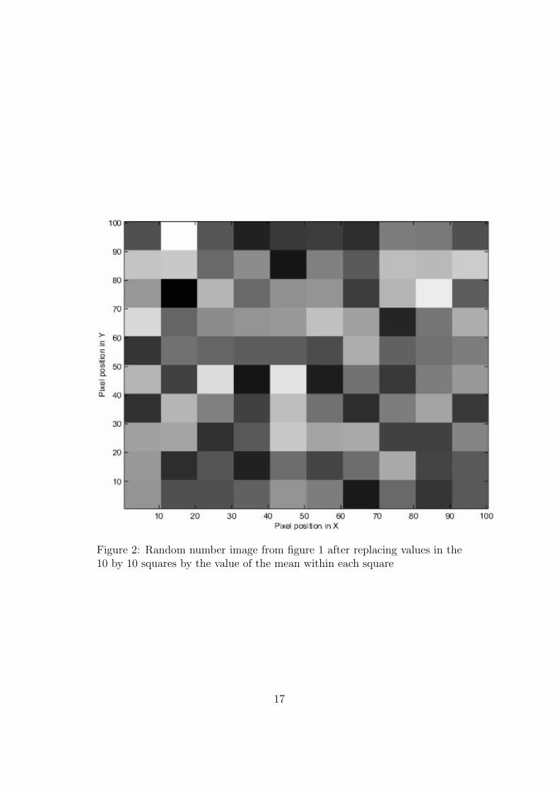
Figure 2: Random number image from figure 1 after replacing values in the10 by 10 squares by the value of the mean within each square

17

Figure 3: Random number image from figure 1 after smoothing with a Gaus-sian smoothing kernel of full width at half maximum of 10 pixels

18

Figure 4: Smoothed random number image from figure 3 after thresholdingat Z = 2.5. Values less than 2.5 have been set to zero (displayed as black).The remaining values have been set to one (displayed as white).

19

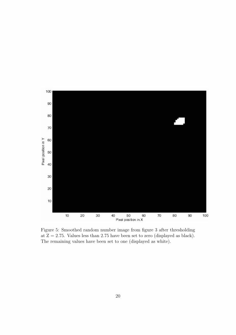
Figure 5: Smoothed random number image from figure 3 after thresholdingat Z = 2.75. Values less than 2.75 have been set to zero (displayed as black).The remaining values have been set to one (displayed as white).

20

Figure 6: Expected EC values for an image of 100 resels.

21

Figure 7: Smoothed random number image from figure 3 with two examplesearch regions: a box (centre) and a frame (outer border of image). X-shapedmarkers are spaced at one resel widths across the image.

22

Figure 8: t threshold giving a FWE rate of 0.05, for spheres of increasingradius. Smoothness was 8mm in X Y and Z directions, and the exampleanalysis had 200 degrees of freedom.

23