Embed Size (px)
Citation preview
Anintroductionto stock-flow
consistentmodels inmacroeco-
nomics
M. R. Grasselli
Introduction
Discrete-timeSFC models
Continuous-time SFCmodels
Extensions
Conclusions
An introduction to stock-flow consistent modelsin macroeconomics
M. R. Grasselli
Mathematics and Statistics - McMaster University
Masterclasses on New Approachesto Economic Challenges
OECD-NAEC, April 17, 2019
Anintroductionto stock-flow
consistentmodels inmacroeco-
nomics
M. R. Grasselli
Introduction
Discrete-timeSFC models
Continuous-time SFCmodels
Extensions
Conclusions
1 Introduction
2 Discrete-time SFC modelsBenchmark model
3 Continuous-time SFC modelsGoodwin modelKeen model
4 ExtensionsStabilizing governmentSpeculationStock PricesGreat ModerationEffective Demand and Inventories
5 Conclusions

Anintroductionto stock-flow
consistentmodels inmacroeco-
nomics
M. R. Grasselli
Introduction
Discrete-timeSFC models
Continuous-time SFCmodels
Extensions
Conclusions
Stock-Flow Consistent models
Stock-flow consistent models emerged in the last decadeas a common language for many heterodox schools ofthought in economics.
They consider both real and monetary factorssimultaneously.
Specify the balance sheet and transactions betweensectors.
Accommodate a number of behavioural assumptions in away that is consistent with the underlying accountingstructure.
Reject the RARE individual (representative agent withrational expectations) in favour of SAFE (sectoral averagewith flexible expectations) modelling.

Anintroductionto stock-flow
consistentmodels inmacroeco-
nomics
M. R. Grasselli
Introduction
Discrete-timeSFC models
Continuous-time SFCmodels
Extensions
Conclusions
Heterodox insight 1: money is not neutral
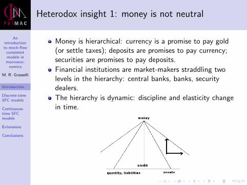
Money is hierarchical: currency is a promise to pay gold(or settle taxes); deposits are promises to pay currency;securities are promises to pay deposits.
Financial institutions are market-makers straddling twolevels in the hierarchy: central banks, banks, securitydealers.
The hierarchy is dynamic: discipline and elasticity changein time.

Anintroductionto stock-flow
consistentmodels inmacroeco-
nomics
M. R. Grasselli
Introduction
Discrete-timeSFC models
Continuous-time SFCmodels
Extensions
Conclusions
Heterodox insight 1: money is not neutral
Money is hierarchical: currency is a promise to pay gold(or settle taxes); deposits are promises to pay currency;securities are promises to pay deposits.
Financial institutions are market-makers straddling twolevels in the hierarchy: central banks, banks, securitydealers.
The hierarchy is dynamic: discipline and elasticity changein time.

Anintroductionto stock-flow
consistentmodels inmacroeco-
nomics
M. R. Grasselli
Introduction
Discrete-timeSFC models
Continuous-time SFCmodels
Extensions
Conclusions
Heterodox insight 2: money is endogenous
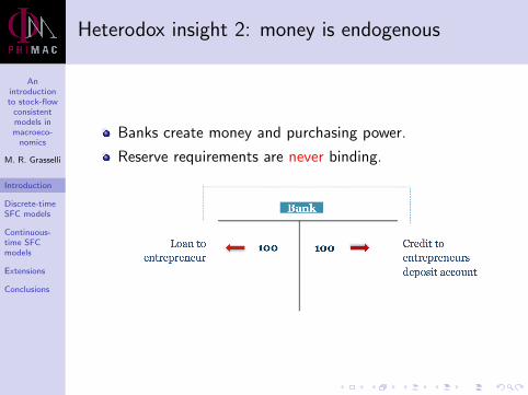
Banks create money and purchasing power.
Reserve requirements are never binding.
Anintroductionto stock-flow
consistentmodels inmacroeco-
nomics
M. R. Grasselli
Introduction
Discrete-timeSFC models
Continuous-time SFCmodels
Extensions
Conclusions
Heterodox insight 2: money is endogenous
Banks create money and purchasing power.
Reserve requirements are never binding.
Anintroductionto stock-flow
consistentmodels inmacroeco-
nomics
M. R. Grasselli
Introduction
Discrete-timeSFC models
Continuous-time SFCmodels
Extensions
Conclusions
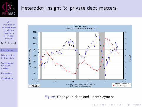
Heterodox insight 3: private debt matters
Figure: Change in debt and unemployment.
Anintroductionto stock-flow
consistentmodels inmacroeco-
nomics
M. R. Grasselli
Introduction
Discrete-timeSFC models
Continuous-time SFCmodels
Extensions
Conclusions
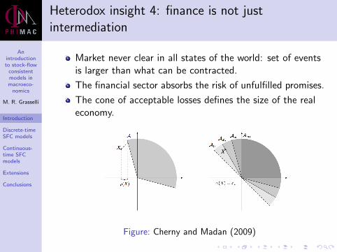
Heterodox insight 4: finance is not justintermediation
Market never clear in all states of the world: set of eventsis larger than what can be contracted.
The financial sector absorbs the risk of unfulfilled promises.
The cone of acceptable losses defines the size of the realeconomy.
Figure: Cherny and Madan (2009)

Anintroductionto stock-flow
consistentmodels inmacroeco-
nomics
M. R. Grasselli
Introduction
Discrete-timeSFC models
Continuous-time SFCmodels
Extensions
Conclusions
Heterodox insight 4: finance is not justintermediation
Market never clear in all states of the world: set of eventsis larger than what can be contracted.
The financial sector absorbs the risk of unfulfilled promises.
The cone of acceptable losses defines the size of the realeconomy.
Figure: Cherny and Madan (2009)
Anintroductionto stock-flow
consistentmodels inmacroeco-
nomics
M. R. Grasselli
Introduction
Discrete-timeSFC models
Benchmarkmodel
Continuous-time SFCmodels
Extensions
Conclusions
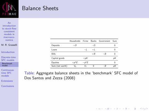
Balance Sheets
Households Firms Banks Government Sum
Deposits +D −D 0
Loans −L +L 0
Bills +B −B 0
Capital goods +pK pK
Equities +peE −peE 0
Sum (net worth) Vh Vf 0 −B pK
Table: Aggregate balance sheets in the ‘benchmark’ SFC model ofDos Santos and Zezza (2008)

Anintroductionto stock-flow
consistentmodels inmacroeco-
nomics
M. R. Grasselli
Introduction
Discrete-timeSFC models
Benchmarkmodel
Continuous-time SFCmodels
Extensions
Conclusions
Transactions
TransactionsHouseholds
FirmsBanks Government Sum
current capital
Consumption −pC +pC 0
Gov spending +pG −pG 0
Investment +pI −pI 0
Acct memo [GDP] [pY ]
Depreciation −pδK +pδK 0
Wages +W −W 0
Taxes −Th −Tf +T 0
Interest on loans −rLt−1Lt−1 +rLt−1Lt−1 0
Interest on bills +rBt−1Bt−1 −rBt−1Bt−1 0
Interest on deposits +rDt−1Dt−1 −rDt−1Dt−1 0
Dividends +Πd + Πb −Πd −Πb 0
Sum Sh Sf −p(I − δK ) 0 Sg 0
Table: Transactions in the ‘benchmark’ SFC model of Dos Santosand Zezza (2008)
Anintroductionto stock-flow
consistentmodels inmacroeco-
nomics
M. R. Grasselli
Introduction
Discrete-timeSFC models
Benchmarkmodel
Continuous-time SFCmodels
Extensions
Conclusions
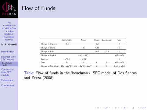
Flow of Funds
Households Firms Banks Government Sum
Change in Deposits +∆D −∆D 0
Change in Loans −∆L +∆L 0
Change in Bills +∆B −∆B 0
Change in Capital +p(I − δK ) p(I − δK )
Equities +pe∆E −pe∆E 0
Sum Sh Sf 0 Sg p(I − δK )
Change in Net Worth (Sh + ∆peE ) (Sf −∆peE + ∆pK ) 0 Sg ∆pK + p∆K
Table: Flow of funds in the ‘benchmark’ SFC model of Dos Santosand Zezza (2008)
Anintroductionto stock-flow
consistentmodels inmacroeco-
nomics
M. R. Grasselli
Introduction
Discrete-timeSFC models
Benchmarkmodel
Continuous-time SFCmodels
Extensions
Conclusions
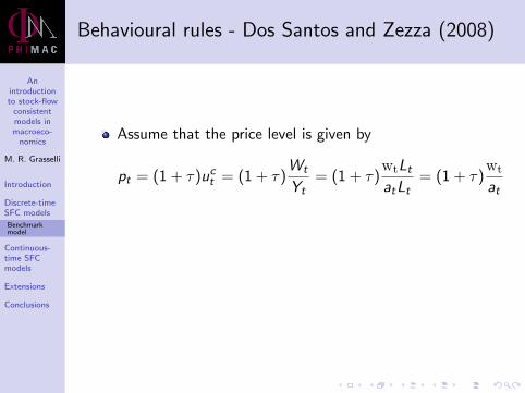
Behavioural rules - Dos Santos and Zezza (2008)
Assume that the price level is given by
pt = (1 + τ)uct = (1 + τ)Wt
Yt= (1 + τ)
wtLtatLt
= (1 + τ)wt
at
It follows that the wage share of nominal output is
ω =Wt
ptYt=
wtLtat(1 + τ)wtYt
=1
1 + τ
and the corresponding profit share is πt = 1− ωt = τ1+τ .
Anintroductionto stock-flow
consistentmodels inmacroeco-
nomics
M. R. Grasselli
Introduction
Discrete-timeSFC models
Benchmarkmodel
Continuous-time SFCmodels
Extensions
Conclusions
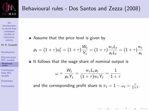
Behavioural rules - Dos Santos and Zezza (2008)
Assume that the price level is given by
pt = (1 + τ)uct = (1 + τ)Wt
Yt= (1 + τ)
wtLtatLt
= (1 + τ)wt
at
It follows that the wage share of nominal output is
ω =Wt
ptYt=
wtLtat(1 + τ)wtYt
=1
1 + τ
and the corresponding profit share is πt = 1− ωt = τ1+τ .
Anintroductionto stock-flow
consistentmodels inmacroeco-
nomics
M. R. Grasselli
Introduction
Discrete-timeSFC models
Benchmarkmodel
Continuous-time SFCmodels
Extensions
Conclusions
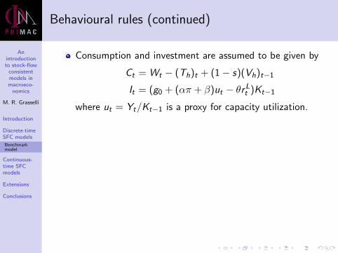
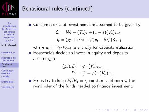
Behavioural rules (continued)
Consumption and investment are assumed to be given by
Ct = Wt − (Th)t + (1− s)(Vh)t−1
It = (g0 + (απ + β)ut − θrLt )Kt−1
where ut = Yt/Kt−1 is a proxy for capacity utilization.
Households decide to invest in equity and depositsaccording to
(pe)tEt = ϕ · (Vh)t−1
Dt = (1− ϕ) · (Vh)t−1
Firms try to keep Et/Kt = χ constant and borrow theremainder of the funds needed to finance investment.Consequently, the equilibrium price for equities is
pet =ϕ · (Vh)tχKt

Anintroductionto stock-flow
consistentmodels inmacroeco-
nomics
M. R. Grasselli
Introduction
Discrete-timeSFC models
Benchmarkmodel
Continuous-time SFCmodels
Extensions
Conclusions
Behavioural rules (continued)
Consumption and investment are assumed to be given by
Ct = Wt − (Th)t + (1− s)(Vh)t−1
It = (g0 + (απ + β)ut − θrLt )Kt−1
where ut = Yt/Kt−1 is a proxy for capacity utilization.Households decide to invest in equity and depositsaccording to
(pe)tEt = ϕ · (Vh)t−1
Dt = (1− ϕ) · (Vh)t−1
Firms try to keep Et/Kt = χ constant and borrow theremainder of the funds needed to finance investment.Consequently, the equilibrium price for equities is
pet =ϕ · (Vh)tχKt
Anintroductionto stock-flow
consistentmodels inmacroeco-
nomics
M. R. Grasselli
Introduction
Discrete-timeSFC models
Benchmarkmodel
Continuous-time SFCmodels
Extensions
Conclusions
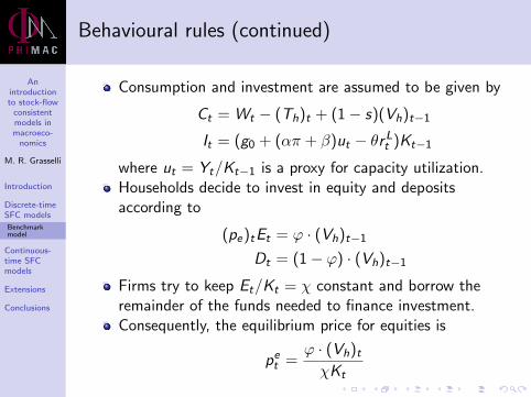
Behavioural rules (continued)
Consumption and investment are assumed to be given by
Ct = Wt − (Th)t + (1− s)(Vh)t−1
It = (g0 + (απ + β)ut − θrLt )Kt−1
where ut = Yt/Kt−1 is a proxy for capacity utilization.Households decide to invest in equity and depositsaccording to
(pe)tEt = ϕ · (Vh)t−1
Dt = (1− ϕ) · (Vh)t−1
Firms try to keep Et/Kt = χ constant and borrow theremainder of the funds needed to finance investment.
Consequently, the equilibrium price for equities is
pet =ϕ · (Vh)tχKt
Anintroductionto stock-flow
consistentmodels inmacroeco-
nomics
M. R. Grasselli
Introduction
Discrete-timeSFC models
Benchmarkmodel
Continuous-time SFCmodels
Extensions
Conclusions
Behavioural rules (continued)
Consumption and investment are assumed to be given by
Ct = Wt − (Th)t + (1− s)(Vh)t−1
It = (g0 + (απ + β)ut − θrLt )Kt−1
where ut = Yt/Kt−1 is a proxy for capacity utilization.Households decide to invest in equity and depositsaccording to
(pe)tEt = ϕ · (Vh)t−1
Dt = (1− ϕ) · (Vh)t−1
Firms try to keep Et/Kt = χ constant and borrow theremainder of the funds needed to finance investment.Consequently, the equilibrium price for equities is
pet =ϕ · (Vh)tχKt

Anintroductionto stock-flow
consistentmodels inmacroeco-
nomics
M. R. Grasselli
Introduction
Discrete-timeSFC models
Benchmarkmodel
Continuous-time SFCmodels
Extensions
Conclusions
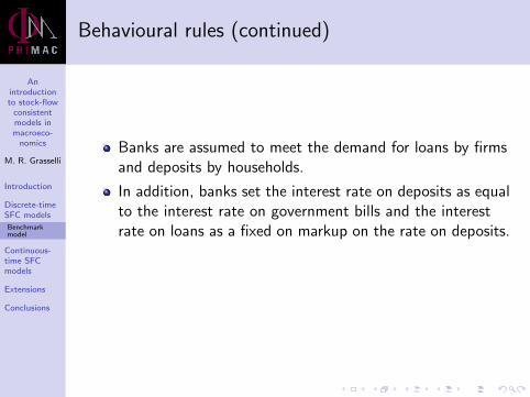
Behavioural rules (continued)
Banks are assumed to meet the demand for loans by firmsand deposits by households.
In addition, banks set the interest rate on deposits as equalto the interest rate on government bills and the interestrate on loans as a fixed on markup on the rate on deposits.
The government chooses the level of spending Gt , theinterest rate rbt and the level of taxes Tt , with the amountof debt determined as a residual.
Anintroductionto stock-flow
consistentmodels inmacroeco-
nomics
M. R. Grasselli
Introduction
Discrete-timeSFC models
Benchmarkmodel
Continuous-time SFCmodels
Extensions
Conclusions
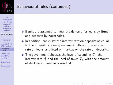
Behavioural rules (continued)
Banks are assumed to meet the demand for loans by firmsand deposits by households.
In addition, banks set the interest rate on deposits as equalto the interest rate on government bills and the interestrate on loans as a fixed on markup on the rate on deposits.
The government chooses the level of spending Gt , theinterest rate rbt and the level of taxes Tt , with the amountof debt determined as a residual.
Anintroductionto stock-flow
consistentmodels inmacroeco-
nomics
M. R. Grasselli
Introduction
Discrete-timeSFC models
Benchmarkmodel
Continuous-time SFCmodels
Extensions
Conclusions
Behavioural rules (continued)
Banks are assumed to meet the demand for loans by firmsand deposits by households.
In addition, banks set the interest rate on deposits as equalto the interest rate on government bills and the interestrate on loans as a fixed on markup on the rate on deposits.
The government chooses the level of spending Gt , theinterest rate rbt and the level of taxes Tt , with the amountof debt determined as a residual.

Anintroductionto stock-flow
consistentmodels inmacroeco-
nomics
M. R. Grasselli
Introduction
Discrete-timeSFC models
Benchmarkmodel
Continuous-time SFCmodels
Extensions
Conclusions
Dynamics
Using the SFC tables and the behavioural rules, one canreduce the dynamics of the model to system of differenceequations for the variables
gt =It
Kt−1bt =
Bt
ptKt
vht =(Vh)tptKt
ut =Yt
Kt−1
It is very difficult to establish the properties of thedynamics analytically, although the model is relatively easyto simulate.
Anintroductionto stock-flow
consistentmodels inmacroeco-
nomics
M. R. Grasselli
Introduction
Discrete-timeSFC models
Continuous-time SFCmodels
Goodwin model
Keen model
Extensions
Conclusions
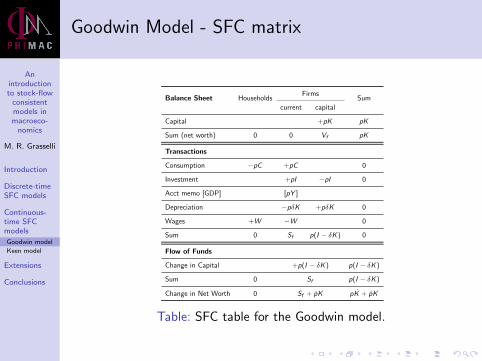
Goodwin Model - SFC matrix
Balance Sheet HouseholdsFirms
Sum
current capital
Capital +pK pK
Sum (net worth) 0 0 Vf pK
Transactions
Consumption −pC +pC 0
Investment +pI −pI 0
Acct memo [GDP] [pY ]
Depreciation −pδK +pδK 0
Wages +W −W 0
Sum 0 Sf p(I − δK ) 0
Flow of Funds
Change in Capital +p(I − δK ) p(I − δK )
Sum 0 Sf p(I − δK )
Change in Net Worth 0 Sf + pK pK + pK
Table: SFC table for the Goodwin model.
Anintroductionto stock-flow
consistentmodels inmacroeco-
nomics
M. R. Grasselli
Introduction
Discrete-timeSFC models
Continuous-time SFCmodels
Goodwin model
Keen model
Extensions
Conclusions
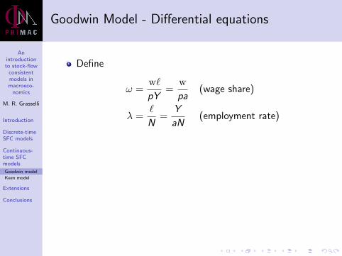
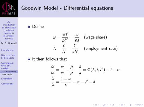
Goodwin Model - Differential equations
Define
ω =w`
pY=
w
pa(wage share)
λ =`
N=
Y
aN(employment rate)
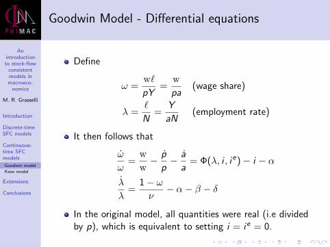
It then follows that
ω
ω=
w
w− p
p− a
a= Φ(λ, i , ie)− i − α
λ
λ=
1− ων− α− β − δ
In the original model, all quantities were real (i.e dividedby p), which is equivalent to setting i = ie = 0.
Anintroductionto stock-flow
consistentmodels inmacroeco-
nomics
M. R. Grasselli
Introduction
Discrete-timeSFC models
Continuous-time SFCmodels
Goodwin model
Keen model
Extensions
Conclusions
Goodwin Model - Differential equations
Define
ω =w`
pY=
w
pa(wage share)
λ =`
N=
Y
aN(employment rate)
It then follows that
ω
ω=
w
w− p
p− a
a= Φ(λ, i , ie)− i − α
λ
λ=
1− ων− α− β − δ
In the original model, all quantities were real (i.e dividedby p), which is equivalent to setting i = ie = 0.
Anintroductionto stock-flow
consistentmodels inmacroeco-
nomics
M. R. Grasselli
Introduction
Discrete-timeSFC models
Continuous-time SFCmodels
Goodwin model
Keen model
Extensions
Conclusions
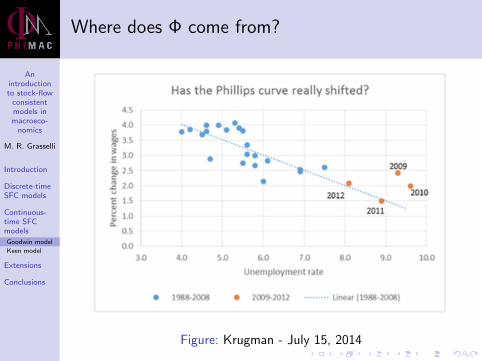
Where does Φ come from?
Figure: Krugman - July 15, 2014
Anintroductionto stock-flow
consistentmodels inmacroeco-
nomics
M. R. Grasselli
Introduction
Discrete-timeSFC models
Continuous-time SFCmodels
Goodwin model
Keen model
Extensions
Conclusions
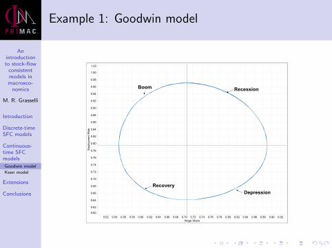
Example 1: Goodwin model
0.52 0.54 0.56 0.58 0.60 0.62 0.64 0.66 0.68 0.70 0.72 0.74 0.76 0.78 0.80 0.82 0.84 0.86 0.88 0.90 0.92Wage Share
0.60
0.62
0.64
0.66
0.68
0.70
0.72
0.74
0.76
0.78
0.80
0.82
0.84
0.86
0.88
0.90
0.92
0.94
0.96
0.98
1.00
1.02
Employment Rate
Boom Recession
DepressionRecovery
Anintroductionto stock-flow
consistentmodels inmacroeco-
nomics
M. R. Grasselli
Introduction
Discrete-timeSFC models
Continuous-time SFCmodels
Goodwin model
Keen model
Extensions
Conclusions
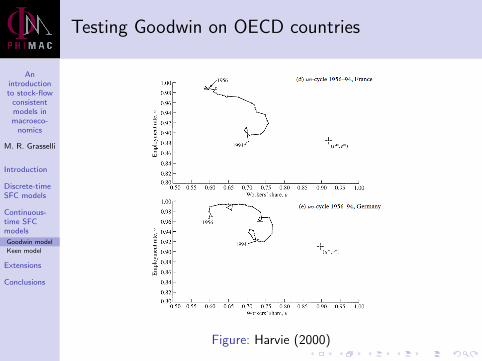
Testing Goodwin on OECD countries
Figure: Harvie (2000)
Anintroductionto stock-flow
consistentmodels inmacroeco-
nomics
M. R. Grasselli
Introduction
Discrete-timeSFC models
Continuous-time SFCmodels
Goodwin model
Keen model
Extensions
Conclusions
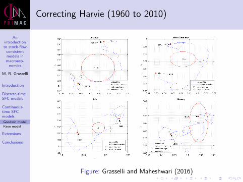
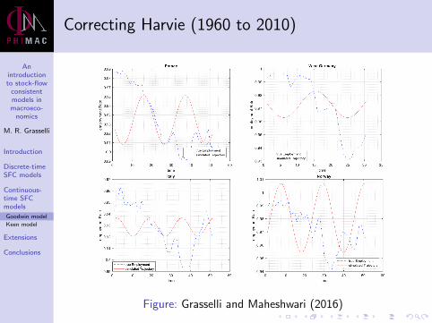
Correcting Harvie (1960 to 2010)
Figure: Grasselli and Maheshwari (2016)
Anintroductionto stock-flow
consistentmodels inmacroeco-
nomics
M. R. Grasselli
Introduction
Discrete-timeSFC models
Continuous-time SFCmodels
Goodwin model
Keen model
Extensions
Conclusions
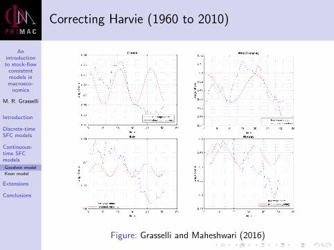
Correcting Harvie (1960 to 2010)
Figure: Grasselli and Maheshwari (2016)
Anintroductionto stock-flow
consistentmodels inmacroeco-
nomics
M. R. Grasselli
Introduction
Discrete-timeSFC models
Continuous-time SFCmodels
Goodwin model
Keen model
Extensions
Conclusions
Correcting Harvie (1960 to 2010)
Figure: Grasselli and Maheshwari (2016)
Anintroductionto stock-flow
consistentmodels inmacroeco-
nomics
M. R. Grasselli
Introduction
Discrete-timeSFC models
Continuous-time SFCmodels
Goodwin model
Keen model
Extensions
Conclusions
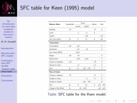
SFC table for Keen (1995) model
Balance Sheet HouseholdsFirms
Banks Sum
current capital
Deposits +D −D 0
Loans −L +L 0
Capital +pK pK
Sum (net worth) Vh 0 Vf 0 pK
Transactions
Consumption −pC +pC 0
Investment +pI −pI 0
Acct memo [GDP] [pY ]
Wages +W −W 0
Depreciation −pδK +pδK 0
Interest on deposits +rD −rD 0
Interest on loans −rL +rL 0
Sum Sh Sf −p(I − δK ) 0 0
Flow of Funds
Change in Deposits +D −D 0
Change in Loans −L +L 0
Change in Capital +p(I − δK ) pI
Sum Sh 0 Sf 0 p(I − δK )
Change in Net Worth Sh (Sf + pK ) pK + pK
Table: SFC table for the Keen model.

Anintroductionto stock-flow
consistentmodels inmacroeco-
nomics
M. R. Grasselli
Introduction
Discrete-timeSFC models
Continuous-time SFCmodels
Goodwin model
Keen model
Extensions
Conclusions
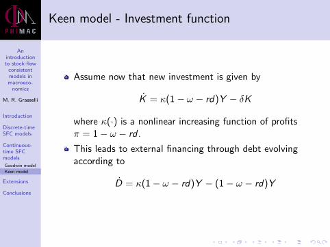
Keen model - Investment function
Assume now that new investment is given by
K = κ(1− ω − rd)Y − δK
where κ(·) is a nonlinear increasing function of profitsπ = 1− ω − rd .
This leads to external financing through debt evolvingaccording to
D = κ(1− ω − rd)Y − (1− ω − rd)Y
Anintroductionto stock-flow
consistentmodels inmacroeco-
nomics
M. R. Grasselli
Introduction
Discrete-timeSFC models
Continuous-time SFCmodels
Goodwin model
Keen model
Extensions
Conclusions
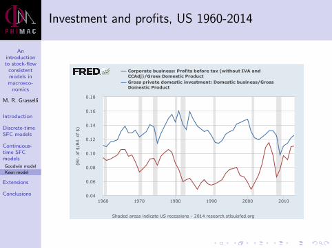
Investment and profits, US 1960-2014
0.04
0.06
0.08
0.10
0.12
0.14
0.16
0.18
1960 1970 1980 1990 2000 2010
ShadedareasindicateUSrecessions-2014research.stlouisfed.org
Corporatebusiness:Profitsbeforetax(withoutIVAandCCAdj)/GrossDomesticProductGrossprivatedomesticinvestment:Domesticbusiness/GrossDomesticProduct
(Bil.
of$/B
il.o
f$)
Anintroductionto stock-flow
consistentmodels inmacroeco-
nomics
M. R. Grasselli
Introduction
Discrete-timeSFC models
Continuous-time SFCmodels
Goodwin model
Keen model
Extensions
Conclusions
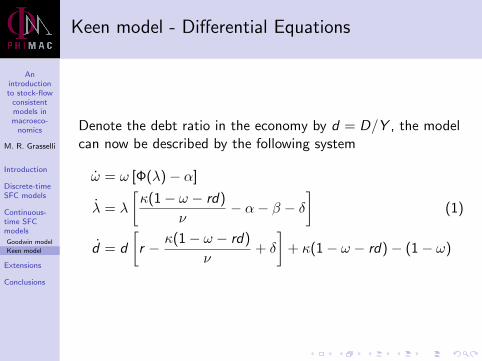
Keen model - Differential Equations
Denote the debt ratio in the economy by d = D/Y , the modelcan now be described by the following system
ω = ω [Φ(λ)− α]
λ = λ
[κ(1− ω − rd)
ν− α− β − δ
](1)
d = d
[r − κ(1− ω − rd)
ν+ δ
]+ κ(1− ω − rd)− (1− ω)
Anintroductionto stock-flow
consistentmodels inmacroeco-
nomics
M. R. Grasselli
Introduction
Discrete-timeSFC models
Continuous-time SFCmodels
Goodwin model
Keen model
Extensions
Conclusions
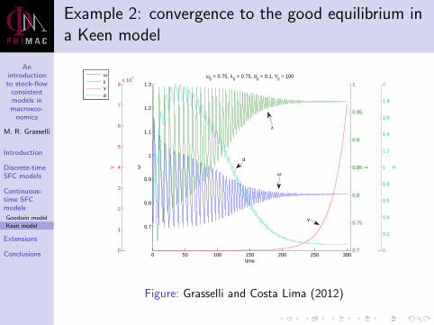
Example 2: convergence to the good equilibrium ina Keen model
0.7
0.75
0.8
0.85
0.9
0.95
1
λ
ωλYd
0
1
2
3
4
5
6
7
8x 10
7
Y
0
0.2
0.4
0.6
0.8
1
1.2
1.4
1.6
1.8
2
d
0 50 100 150 200 250 300
0.7
0.8
0.9
1
1.1
1.2
1.3
time
ω
ω0 = 0.75, λ
0 = 0.75, d
0 = 0.1, Y
0 = 100
d
λ
ω
Y
Figure: Grasselli and Costa Lima (2012)
Anintroductionto stock-flow
consistentmodels inmacroeco-
nomics
M. R. Grasselli
Introduction
Discrete-timeSFC models
Continuous-time SFCmodels
Goodwin model
Keen model
Extensions
Conclusions
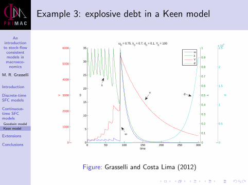
Example 3: explosive debt in a Keen model
0
0.1
0.2
0.3
0.4
0.5
0.6
0.7
0.8
0.9
1
λ
0
1000
2000
3000
4000
5000
6000
Y
0
0.5
1
1.5
2
2.5x 10
6
d
0 50 100 150 200 250 3000
5
10
15
20
25
30
35
time
ω
ω0 = 0.75, λ
0 = 0.7, d
0 = 0.1, Y
0 = 100
ωλYd
λ
Y d
ω
Figure: Grasselli and Costa Lima (2012)
Anintroductionto stock-flow
consistentmodels inmacroeco-
nomics
M. R. Grasselli
Introduction
Discrete-timeSFC models
Continuous-time SFCmodels
Goodwin model
Keen model
Extensions
Conclusions
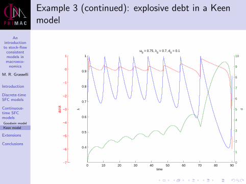
Example 3 (continued): explosive debt in a Keenmodel
0
1
2
3
4
5
6
7
8
9
10
d
−7
−6
−5
−4
−3
−2
−1
0
1dd
/dt
0 10 20 30 40 50 60 70 80 90
0.4
0.5
0.6
0.7
0.8
0.9
1
time
λ
ω0 = 0.75, λ
0 = 0.7, d
0 = 0.1
Anintroductionto stock-flow
consistentmodels inmacroeco-
nomics
M. R. Grasselli
Introduction
Discrete-timeSFC models
Continuous-time SFCmodels
Goodwin model
Keen model
Extensions
Conclusions
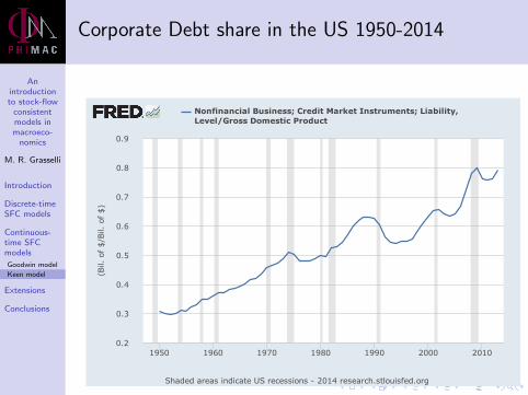
Corporate Debt share in the US 1950-2014
0.2
0.3
0.4
0.5
0.6
0.7
0.8
0.9
1950 1960 1970 1980 1990 2000 2010
ShadedareasindicateUSrecessions-2014research.stlouisfed.org
NonfinancialBusiness;CreditMarketInstruments;Liability,Level/GrossDomesticProduct
(Bil.of$/Bil.of$)
Anintroductionto stock-flow
consistentmodels inmacroeco-
nomics
M. R. Grasselli
Introduction
Discrete-timeSFC models
Continuous-time SFCmodels
Goodwin model
Keen model
Extensions
Conclusions
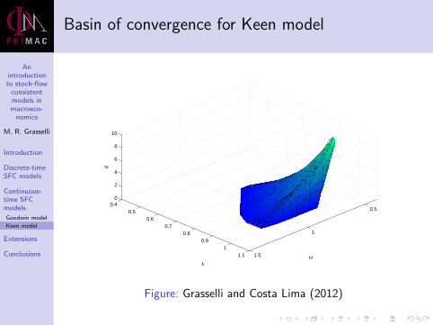
Basin of convergence for Keen model
0.5
1
1.5
0.40.5
0.60.7
0.80.9
11.1
0
2
4
6
8
10
ωλ
d
Figure: Grasselli and Costa Lima (2012)
Anintroductionto stock-flow
consistentmodels inmacroeco-
nomics
M. R. Grasselli
Introduction
Discrete-timeSFC models
Continuous-time SFCmodels
Goodwin model
Keen model
Extensions
Conclusions
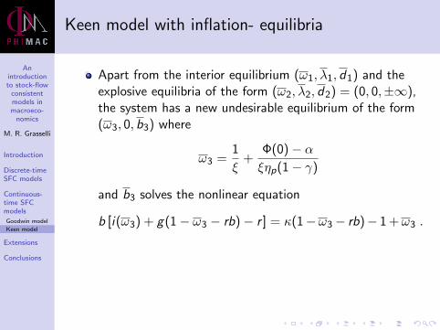
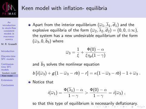
Keen model with inflation- equilibria
Apart from the interior equilibrium (ω1, λ1, d1) and theexplosive equilibria of the form (ω2, λ2, d2) = (0, 0,±∞),the system has a new undesirable equilibrium of the form(ω3, 0, b3) where
ω3 =1
ξ+
Φ(0)− αξηp(1− γ)
and b3 solves the nonlinear equation
b [i(ω3) + g(1− ω3 − rb)− r ] = κ(1−ω3− rb)− 1 +ω3 .
Notice that
i(ω1) =Φ(λ1)− α
1− γ>
Φ(0)− α1− γ
= i(ω3) ,
so that this type of equilibrium is necessarily deflationary.
Anintroductionto stock-flow
consistentmodels inmacroeco-
nomics
M. R. Grasselli
Introduction
Discrete-timeSFC models
Continuous-time SFCmodels
Goodwin model
Keen model
Extensions
Conclusions
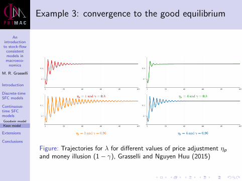
Example 3: convergence to the good equilibrium
Figure: Trajectories for λ for different values of price adjustment ηpand money illusion (1− γ), Grasselli and Nguyen Huu (2015)
Anintroductionto stock-flow
consistentmodels inmacroeco-
nomics
M. R. Grasselli
Introduction
Discrete-timeSFC models
Continuous-time SFCmodels
Goodwin model
Keen model
Extensions
Conclusions
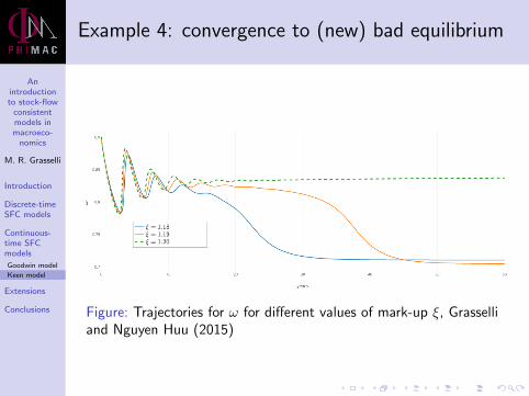
Example 4: convergence to (new) bad equilibrium
Figure: Trajectories for ω for different values of mark-up ξ, Grasselliand Nguyen Huu (2015)
Anintroductionto stock-flow
consistentmodels inmacroeco-
nomics
M. R. Grasselli
Introduction
Discrete-timeSFC models
Continuous-time SFCmodels
Goodwin model
Keen model
Extensions
Conclusions
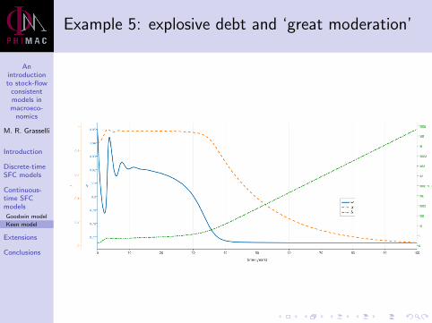
Example 5: explosive debt and ‘great moderation’
Anintroductionto stock-flow
consistentmodels inmacroeco-
nomics
M. R. Grasselli
Introduction
Discrete-timeSFC models
Continuous-time SFCmodels
Extensions
Stabilizinggovernment
Speculation
Stock Prices
GreatModeration
EffectiveDemand andInventories
Conclusions
Introducing a government sector
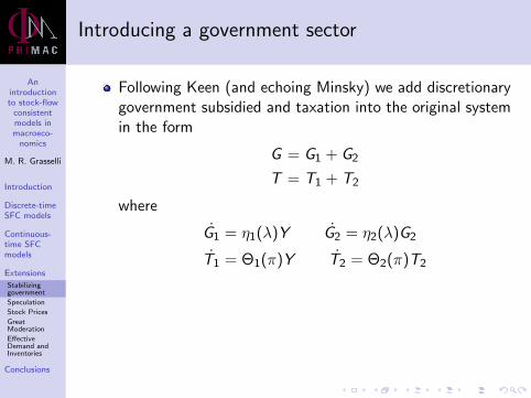
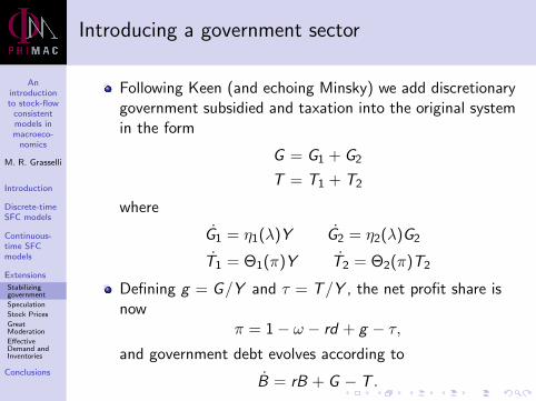
Following Keen (and echoing Minsky) we add discretionarygovernment subsidied and taxation into the original systemin the form
G = G1 + G2
T = T1 + T2
where
G1 = η1(λ)Y G2 = η2(λ)G2
T1 = Θ1(π)Y T2 = Θ2(π)T2
Defining g = G/Y and τ = T/Y , the net profit share isnow
π = 1− ω − rd + g − τ,and government debt evolves according to
B = rB + G − T .
Anintroductionto stock-flow
consistentmodels inmacroeco-
nomics
M. R. Grasselli
Introduction
Discrete-timeSFC models
Continuous-time SFCmodels
Extensions
Stabilizinggovernment
Speculation
Stock Prices
GreatModeration
EffectiveDemand andInventories
Conclusions
Introducing a government sector
Following Keen (and echoing Minsky) we add discretionarygovernment subsidied and taxation into the original systemin the form
G = G1 + G2
T = T1 + T2
where
G1 = η1(λ)Y G2 = η2(λ)G2
T1 = Θ1(π)Y T2 = Θ2(π)T2
Defining g = G/Y and τ = T/Y , the net profit share isnow
π = 1− ω − rd + g − τ,and government debt evolves according to
B = rB + G − T .
Anintroductionto stock-flow
consistentmodels inmacroeco-
nomics
M. R. Grasselli
Introduction
Discrete-timeSFC models
Continuous-time SFCmodels
Extensions
Stabilizinggovernment
Speculation
Stock Prices
GreatModeration
EffectiveDemand andInventories
Conclusions
Good equilibrium
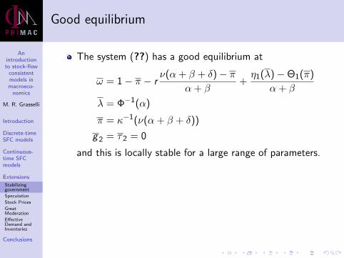
The system (??) has a good equilibrium at
ω = 1− π − rν(α + β + δ)− π
α + β+η1(λ)−Θ1(π)
α + β
λ = Φ−1(α)
π = κ−1(ν(α + β + δ))
g2 = τ2 = 0
and this is locally stable for a large range of parameters.
The other variables then converge exponentially fast to
d =ν(α + β + δ)− π
α + β
g1 =η1(λ)
α + β
τ1 =Θ1(π)
α + β
Anintroductionto stock-flow
consistentmodels inmacroeco-
nomics
M. R. Grasselli
Introduction
Discrete-timeSFC models
Continuous-time SFCmodels
Extensions
Stabilizinggovernment
Speculation
Stock Prices
GreatModeration
EffectiveDemand andInventories
Conclusions
Good equilibrium
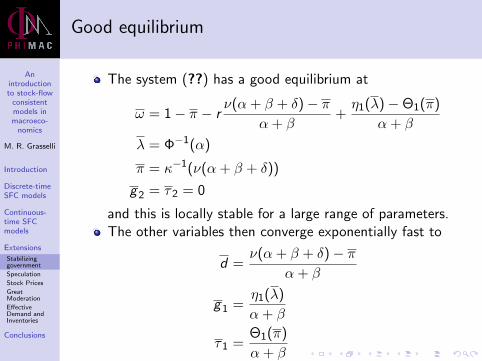
The system (??) has a good equilibrium at
ω = 1− π − rν(α + β + δ)− π
α + β+η1(λ)−Θ1(π)
α + β
λ = Φ−1(α)
π = κ−1(ν(α + β + δ))
g2 = τ2 = 0
and this is locally stable for a large range of parameters.The other variables then converge exponentially fast to
d =ν(α + β + δ)− π
α + β
g1 =η1(λ)
α + β
τ1 =Θ1(π)
α + β
Anintroductionto stock-flow
consistentmodels inmacroeco-
nomics
M. R. Grasselli
Introduction
Discrete-timeSFC models
Continuous-time SFCmodels
Extensions
Stabilizinggovernment
Speculation
Stock Prices
GreatModeration
EffectiveDemand andInventories
Conclusions
Bad equilibria - destabilizing a stable crisis
Recall that π = 1− ω − rd + g − τ .
The system has bad equilibria of the form
(ω, λ, g2, τ2, π) = (0, 0, 0, 0,−∞)
(ω, λ, g2, τ2, π) = (0, 0,±∞, 0,−∞)
If g2(0) > 0, then any equilibria with π → −∞ is locallyunstable provided η2(0) > r .
On the other hand, if g2(0) < 0 (austerity), then theseequilibria are all locally stable.
Anintroductionto stock-flow
consistentmodels inmacroeco-
nomics
M. R. Grasselli
Introduction
Discrete-timeSFC models
Continuous-time SFCmodels
Extensions
Stabilizinggovernment
Speculation
Stock Prices
GreatModeration
EffectiveDemand andInventories
Conclusions
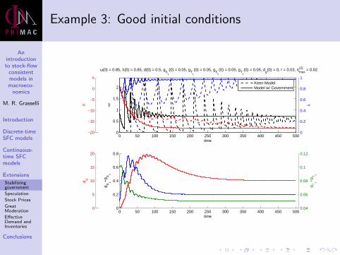
Example 3: Good initial conditions
0
0.2
0.4
0.6
0.8
1
λ
−20
−15
−10
−5
0
5d
0 50 100 150 200 250 300 350 400 450 5000
0.5
1
1.5
2
time
ω
ω(0) = 0.85, λ(0) = 0.85, d(0) = 0.5, gS
1
(0) = 0.05, gT
1
(0) = 0.05, gS
2
(0) = 0.05, gT
2
(0) = 0.05, dg(0) = 0, r = 0.03, η
max(2) = 0.02
Keen ModelModel w/ Government
0.04
0.06
0.08
0.1
0.12
g T1+
g T2
0
5
10
15
20
d g
0 50 100 150 200 250 300 350 400 450 5000
0.2
0.4
0.6
0.8
time
g S1+
g S2
Anintroductionto stock-flow
consistentmodels inmacroeco-
nomics
M. R. Grasselli
Introduction
Discrete-timeSFC models
Continuous-time SFCmodels
Extensions
Stabilizinggovernment
Speculation
Stock Prices
GreatModeration
EffectiveDemand andInventories
Conclusions
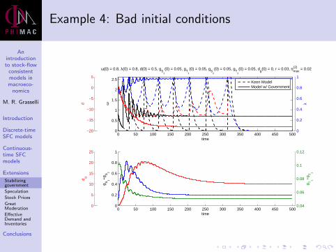
Example 4: Bad initial conditions
0
0.2
0.4
0.6
0.8
1
λ
−20
−15
−10
−5
0
5d
0 50 100 150 200 250 300 350 400 450 5000
0.5
1
1.5
2
2.5
time
ω
ω(0) = 0.8, λ(0) = 0.8, d(0) = 0.5, gS
1
(0) = 0.05, gT
1
(0) = 0.05, gS
2
(0) = 0.05, gT
2
(0) = 0.05, dg(0) = 0, r = 0.03, η
max(2) = 0.02
Keen ModelModel w/ Government
0.04
0.06
0.08
0.1
0.12
g T1+
g T2
0
5
10
15
20
25
d g
0 50 100 150 200 250 300 350 400 450 5000
0.2
0.4
0.6
0.8
1
time
g S1+
g S2
Anintroductionto stock-flow
consistentmodels inmacroeco-
nomics
M. R. Grasselli
Introduction
Discrete-timeSFC models
Continuous-time SFCmodels
Extensions
Stabilizinggovernment
Speculation
Stock Prices
GreatModeration
EffectiveDemand andInventories
Conclusions
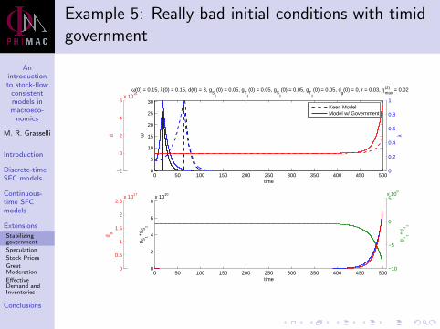
Example 5: Really bad initial conditions with timidgovernment
0
0.2
0.4
0.6
0.8
1
λ
−2
0
2
4
6x 10
16
d
0 50 100 150 200 250 300 350 400 450 5000
5
10
15
20
25
30
time
ω
ω(0) = 0.15, λ(0) = 0.15, d(0) = 3, gS
1
(0) = 0.05, gT
1
(0) = 0.05, gS
2
(0) = 0.05, gT
2
(0) = 0.05, dg(0) = 0, r = 0.03, η
max(2) = 0.02
Keen ModelModel w/ Government
−10
−5
0
5x 10
8
g T1+
g T2
0
0.5
1
1.5
2
2.5x 10
17
d g
0 50 100 150 200 250 300 350 400 450 5000
2
4
6
8x 10
10
time
g S1+
g S2
Anintroductionto stock-flow
consistentmodels inmacroeco-
nomics
M. R. Grasselli
Introduction
Discrete-timeSFC models
Continuous-time SFCmodels
Extensions
Stabilizinggovernment
Speculation
Stock Prices
GreatModeration
EffectiveDemand andInventories
Conclusions
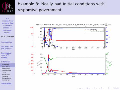
Example 6: Really bad initial conditions withresponsive government
0
0.2
0.4
0.6
0.8
1
λ
−10
−5
0
5x 10
8
g T1+
g T2
0
0.2
0.4
0.6
0.8
1
λ
−500
0
500
1000d
0 50 100 150 200 250 300 350 400 450 5000
5
10
15
20
25
30
time
ω
ω(0) = 0.15, λ(0) = 0.15, d(0) = 3, gS
1
(0) = 0.05, gT
1
(0) = 0.05, gS
2
(0) = 0.05, gT
2
(0) = 0.05, dg(0) = 0, r = 0.03, η
max(2) = 0.2
Keen ModelModel w/ Government
−2
−1.5
−1
−0.5
0
0.5
g T1+
g T2
0
100
200
300
400
500
600
d g
0 50 100 150 200 250 300 350 400 450 5000
5
10
15
20
25
30
time
g S1+
g S2
Anintroductionto stock-flow
consistentmodels inmacroeco-
nomics
M. R. Grasselli
Introduction
Discrete-timeSFC models
Continuous-time SFCmodels
Extensions
Stabilizinggovernment
Speculation
Stock Prices
GreatModeration
EffectiveDemand andInventories
Conclusions
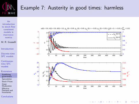
Example 7: Austerity in good times: harmless
0
0.2
0.4
0.6
0.8
1
λ
−20
−15
−10
−5
0d
0 50 100 150 200 250 300 350 400 450 5000
0.5
1
1.5
2
2.5
time
ω
ω(0) = 0.8, λ(0) = 0.8, d(0) = 0.5, gS
1
(0) = 0.05, gT
1
(0) = 0.05, gS
2
(0) = +−0.05, gT
2
(0) = 0.05, dg(0) = 0, r = 0.03, η
max(2) = 0.02
g
S2
(0)>0
gS
2
(0)<0
0.04
0.06
0.08
0.1
0.12
g T1+
g T2
−5
0
5
10
15
20
d g
0 50 100 150 200 250 300 350 400 450 5000
0.2
0.4
0.6
0.8
1
time
g S1+
g S2
Anintroductionto stock-flow
consistentmodels inmacroeco-
nomics
M. R. Grasselli
Introduction
Discrete-timeSFC models
Continuous-time SFCmodels
Extensions
Stabilizinggovernment
Speculation
Stock Prices
GreatModeration
EffectiveDemand andInventories
Conclusions
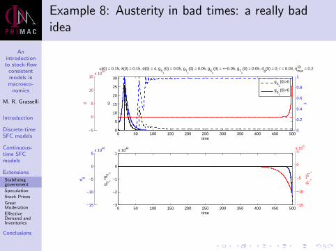
Example 8: Austerity in bad times: a really badidea
0
0.2
0.4
0.6
0.8
1
λ
−5
0
5
10
15x 10
48
d
0 50 100 150 200 250 300 350 400 450 5000
5
10
15
20
25
30
time
ω
ω(0) = 0.15, λ(0) = 0.15, d(0) = 4, gS
1
(0) = 0.05, gT
1
(0) = 0.05, gS
2
(0) = +−0.05, gT
2
(0) = 0.05, dg(0) = 0, r = 0.03, η
max(2) = 0.2
g
S2
(0)>0
gS
2
(0)<0
−15
−10
−5
0
5x 10
8
g T1+
g T2
−15
−10
−5
0
5x 10
48
d g
0 50 100 150 200 250 300 350 400 450 500−3
−2
−1
0
1x 10
48
time
g S1+
g S2
Anintroductionto stock-flow
consistentmodels inmacroeco-
nomics
M. R. Grasselli
Introduction
Discrete-timeSFC models
Continuous-time SFCmodels
Extensions
Stabilizinggovernment
Speculation
Stock Prices
GreatModeration
EffectiveDemand andInventories
Conclusions
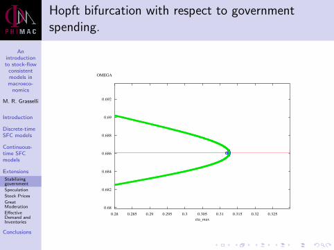
Hopft bifurcation with respect to governmentspending.
0.68
0.682
0.684
0.686
0.688
0.69
0.692
OMEGA
0.28 0.285 0.29 0.295 0.3 0.305 0.31 0.315 0.32 0.325eta_max
Anintroductionto stock-flow
consistentmodels inmacroeco-
nomics
M. R. Grasselli
Introduction
Discrete-timeSFC models
Continuous-time SFCmodels
Extensions
Stabilizinggovernment
Speculation
Stock Prices
GreatModeration
EffectiveDemand andInventories
Conclusions
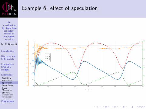
Speculative flow
To introduce the destabilizing effect of purely speculativeinvestment, we consider a modified version of the previousmodel with
L = pI + rLL− κLL + F
Df = pY −W + rfDf − κLL + F
where F denotes a speculative flow modelled by
F = Ψ(g(π) + i(ω))pY ,
where Ψ() is an increasing function of the nominal growth ratein the economy. Notice that this still satisfies
L− Df = pI − Π.
Anintroductionto stock-flow
consistentmodels inmacroeco-
nomics
M. R. Grasselli
Introduction
Discrete-timeSFC models
Continuous-time SFCmodels
Extensions
Stabilizinggovernment
Speculation
Stock Prices
GreatModeration
EffectiveDemand andInventories
Conclusions
Example 6: effect of speculation
Anintroductionto stock-flow
consistentmodels inmacroeco-
nomics
M. R. Grasselli
Introduction
Discrete-timeSFC models
Continuous-time SFCmodels
Extensions
Stabilizinggovernment
Speculation
Stock Prices
GreatModeration
EffectiveDemand andInventories
Conclusions
Stock prices
Consider a stock price process of the form
dStSt
= rbdt + σdWt + γµtdt − γdN(µt)
where Nt is a Cox process with stochastic intensityµt = M(p(t)).
The interest rate for private debt is modelled asrt = rb + rp(t) where
rp(t) = ρ1(St + ρ2)ρ3
Anintroductionto stock-flow
consistentmodels inmacroeco-
nomics
M. R. Grasselli
Introduction
Discrete-timeSFC models
Continuous-time SFCmodels
Extensions
Stabilizinggovernment
Speculation
Stock Prices
GreatModeration
EffectiveDemand andInventories
Conclusions
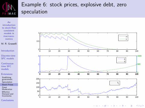
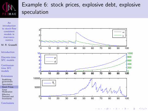
Example 6: stock prices, explosive debt, zerospeculation
0 10 20 30 40 50 60 70 80 90 1000
0.5
1
ωλ
0 10 20 30 40 50 60 70 80 90 1000
1
2
0 10 20 30 40 50 60 70 80 90 1000
500
1000
pd
0 10 20 30 40 50 60 70 80 90 1000
50
100
150
200
St
Anintroductionto stock-flow
consistentmodels inmacroeco-
nomics
M. R. Grasselli
Introduction
Discrete-timeSFC models
Continuous-time SFCmodels
Extensions
Stabilizinggovernment
Speculation
Stock Prices
GreatModeration
EffectiveDemand andInventories
Conclusions
Example 6: stock prices, explosive debt, explosivespeculation
0 10 20 30 40 50 60 70 80 90 1000
1
2
3
ω
λ
0 10 20 30 40 50 60 70 80 90 10002468
10
0 10 20 30 40 50 60 70 80 90 10002004006008001000
pd
0 10 20 30 40 50 60 70 80 90 1000
5000
10000
St
Anintroductionto stock-flow
consistentmodels inmacroeco-
nomics
M. R. Grasselli
Introduction
Discrete-timeSFC models
Continuous-time SFCmodels
Extensions
Stabilizinggovernment
Speculation
Stock Prices
GreatModeration
EffectiveDemand andInventories
Conclusions
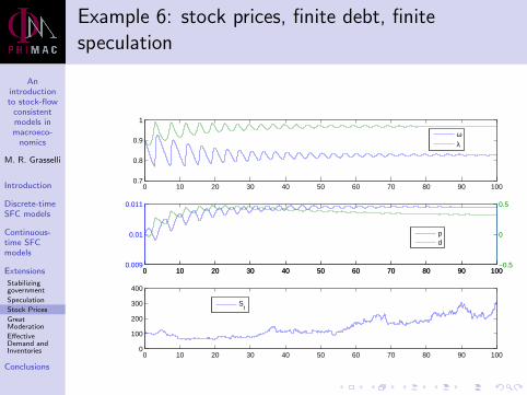
Example 6: stock prices, finite debt, finitespeculation
0 10 20 30 40 50 60 70 80 90 1000.7
0.8
0.9
1
ωλ
0 10 20 30 40 50 60 70 80 90 1000.009
0.01
0.011
0 10 20 30 40 50 60 70 80 90 100−0.5
0
0.5
pd
0 10 20 30 40 50 60 70 80 90 1000
100
200
300
400
St
Anintroductionto stock-flow
consistentmodels inmacroeco-
nomics
M. R. Grasselli
Introduction
Discrete-timeSFC models
Continuous-time SFCmodels
Extensions
Stabilizinggovernment
Speculation
Stock Prices
GreatModeration
EffectiveDemand andInventories
Conclusions
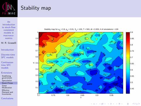
Stability map
0.5
0.5
0.55
0.55
0.55
0.55
0.55
0.55
0.55
0.550.550.
55
0.6
0.6
0.6
0.6
0.6
0.6
0.6
0.6
0.65
0.65
0.65
0.65 0.65
0.65
0.65
0.65
0.7
0.7
0.7
0.7
0.7
0.75
0.75
0.8
0.8
0.85
0.85
0.5
0.55
0.55
0.55
0.6
0.6
0.55
0.6
0.55
0.50.6
0.6
0.5
0.6
0.65
0.55
0.9
0.55
0.6
0.7
0.5
0.55
0.55
0.65
0.6
0.65 0.60.7
0.7
0.65
0.8
0.6
0.6
0.6
0.60.6
0.6
0.45 0.
5
0.45
0.6
0.55
0.7
0.5
0.8
0.65
0.5
0.6
0.7
0.5
0.5
0.6
0.6
λ
d
Stability map for ω0 = 0.8, p
0 = 0.01, S
0 = 100, T = 500, dt = 0.005, # of simulations = 100
0.7 0.75 0.8 0.85 0.9 0.950
0.1
0.2
0.3
0.4
0.5
0.6
0.7
0.8
0.9
1
0.45
0.5
0.55
0.6
0.65
0.7
0.75
0.8
0.85
0.9
Anintroductionto stock-flow
consistentmodels inmacroeco-
nomics
M. R. Grasselli
Introduction
Discrete-timeSFC models
Continuous-time SFCmodels
Extensions
Stabilizinggovernment
Speculation
Stock Prices
GreatModeration
EffectiveDemand andInventories
Conclusions
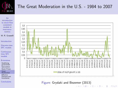
The Great Moderation in the U.S. - 1984 to 2007
Figure: Grydaki and Bezemer (2013)
Anintroductionto stock-flow
consistentmodels inmacroeco-
nomics
M. R. Grasselli
Introduction
Discrete-timeSFC models
Continuous-time SFCmodels
Extensions
Stabilizinggovernment
Speculation
Stock Prices
GreatModeration
EffectiveDemand andInventories
Conclusions
Possible explanations
Real-sector causes: inventory management, labour marketchanges, responses to oil shocks, external balances , etc.
Financial-sector causes: credit accelerator models, financialinnovation, deregulation, better monetary policy, etc.
Grydaki and Bezemer (2013): growth of debt in the realsector.
Anintroductionto stock-flow
consistentmodels inmacroeco-
nomics
M. R. Grasselli
Introduction
Discrete-timeSFC models
Continuous-time SFCmodels
Extensions
Stabilizinggovernment
Speculation
Stock Prices
GreatModeration
EffectiveDemand andInventories
Conclusions
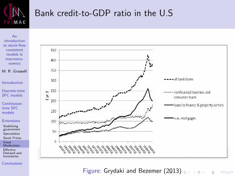
Bank credit-to-GDP ratio in the U.S
Figure: Grydaki and Bezemer (2013)
Anintroductionto stock-flow
consistentmodels inmacroeco-
nomics
M. R. Grasselli
Introduction
Discrete-timeSFC models
Continuous-time SFCmodels
Extensions
Stabilizinggovernment
Speculation
Stock Prices
GreatModeration
EffectiveDemand andInventories
Conclusions
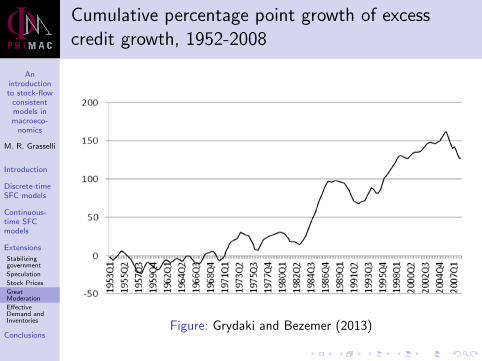
Cumulative percentage point growth of excesscredit growth, 1952-2008
Figure: Grydaki and Bezemer (2013)
Anintroductionto stock-flow
consistentmodels inmacroeco-
nomics
M. R. Grasselli
Introduction
Discrete-timeSFC models
Continuous-time SFCmodels
Extensions
Stabilizinggovernment
Speculation
Stock Prices
GreatModeration
EffectiveDemand andInventories
Conclusions
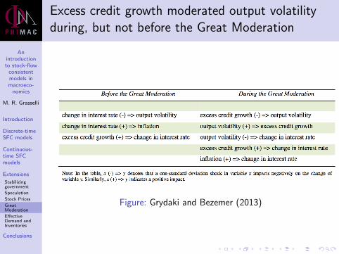
Excess credit growth moderated output volatilityduring, but not before the Great Moderation
Figure: Grydaki and Bezemer (2013)
Anintroductionto stock-flow
consistentmodels inmacroeco-
nomics
M. R. Grasselli
Introduction
Discrete-timeSFC models
Continuous-time SFCmodels
Extensions
Stabilizinggovernment
Speculation
Stock Prices
GreatModeration
EffectiveDemand andInventories
Conclusions
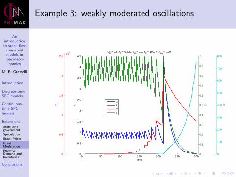
Example 3: weakly moderated oscillations
0
0.1
0.2
0.3
0.4
0.5
0.6
0.7
0.8
0.9
1
λ
0
0.5
1
1.5
2
2.5x 10
6
Y
0
100
200
300
400
500
600
700
800
d
0 50 100 150 200 250 3000
0.5
1
1.5
2
2.5
3
3.5
4
4.5
time
ω
ω0 = 0.8, λ
0 = 0.722, d
0 = 0.1, Y
0 = 100, κ’(π
eq) = 100
ωλYd
Anintroductionto stock-flow
consistentmodels inmacroeco-
nomics
M. R. Grasselli
Introduction
Discrete-timeSFC models
Continuous-time SFCmodels
Extensions
Stabilizinggovernment
Speculation
Stock Prices
GreatModeration
EffectiveDemand andInventories
Conclusions
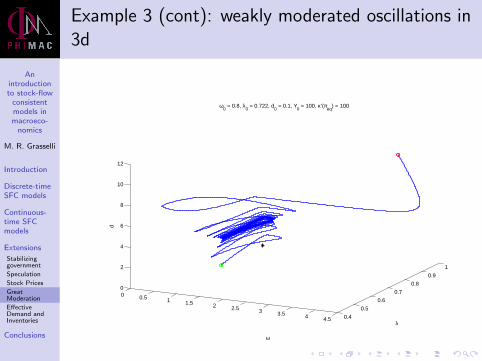
Example 3 (cont): weakly moderated oscillations in3d
0 0.5 1 1.5 2 2.5 3 3.5 4 4.5 0.4
0.5
0.6
0.7
0.8
0.9
1
0
2
4
6
8
10
12
λ
ω0 = 0.8, λ
0 = 0.722, d
0 = 0.1, Y
0 = 100, κ’(π
eq) = 100
ω
d
Anintroductionto stock-flow
consistentmodels inmacroeco-
nomics
M. R. Grasselli
Introduction
Discrete-timeSFC models
Continuous-time SFCmodels
Extensions
Stabilizinggovernment
Speculation
Stock Prices
GreatModeration
EffectiveDemand andInventories
Conclusions
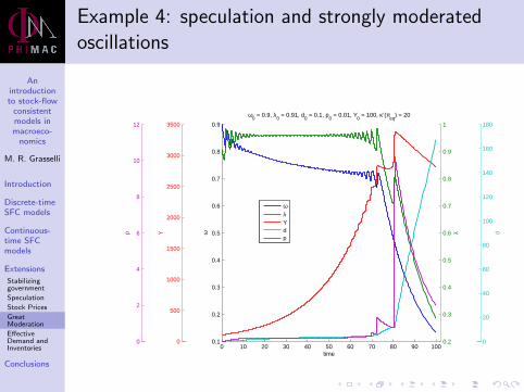
Example 4: speculation and strongly moderatedoscillations
0.2
0.3
0.4
0.5
0.6
0.7
0.8
0.9
1
λ
0
500
1000
1500
2000
2500
3000
3500
Y
0
20
40
60
80
100
120
140
160
180
d
0
2
4
6
8
10
12p
0 10 20 30 40 50 60 70 80 90 1000.1
0.2
0.3
0.4
0.5
0.6
0.7
0.8
0.9
time
ω
ω0 = 0.9, λ
0 = 0.91, d
0 = 0.1, p
0 = 0.01, Y
0 = 100, κ’(π
eq) = 20
ωλYdp
Anintroductionto stock-flow
consistentmodels inmacroeco-
nomics
M. R. Grasselli
Introduction
Discrete-timeSFC models
Continuous-time SFCmodels
Extensions
Stabilizinggovernment
Speculation
Stock Prices
GreatModeration
EffectiveDemand andInventories
Conclusions
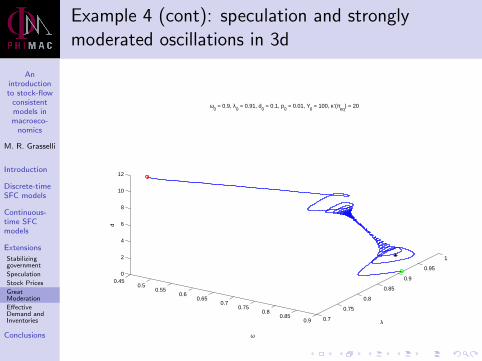
Example 4 (cont): speculation and stronglymoderated oscillations in 3d
0.450.5
0.550.6
0.650.7
0.750.8
0.850.9 0.7
0.75
0.8
0.85
0.9
0.95
1
0
2
4
6
8
10
12
λ
ω0 = 0.9, λ
0 = 0.91, d
0 = 0.1, p
0 = 0.01, Y
0 = 100, κ’(π
eq) = 20
ω
d
Anintroductionto stock-flow
consistentmodels inmacroeco-
nomics
M. R. Grasselli
Introduction
Discrete-timeSFC models
Continuous-time SFCmodels
Extensions
Stabilizinggovernment
Speculation
Stock Prices
GreatModeration
EffectiveDemand andInventories
Conclusions
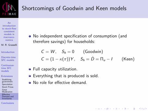
Shortcomings of Goodwin and Keen models
No independent specification of consumption (andtherefore savings) for households:
C = W , Sh = 0 (Goodwin)
C = (1− κ(π))Y , Sh = D = Πu − I (Keen)
Full capacity utilization.
Everything that is produced is sold.
No role for effective demand.
No inventory dynamics.
Anintroductionto stock-flow
consistentmodels inmacroeco-
nomics
M. R. Grasselli
Introduction
Discrete-timeSFC models
Continuous-time SFCmodels
Extensions
Stabilizinggovernment
Speculation
Stock Prices
GreatModeration
EffectiveDemand andInventories
Conclusions
Shortcomings of Goodwin and Keen models
No independent specification of consumption (andtherefore savings) for households:
C = W , Sh = 0 (Goodwin)
C = (1− κ(π))Y , Sh = D = Πu − I (Keen)
Full capacity utilization.
Everything that is produced is sold.
No role for effective demand.
No inventory dynamics.
Anintroductionto stock-flow
consistentmodels inmacroeco-
nomics
M. R. Grasselli
Introduction
Discrete-timeSFC models
Continuous-time SFCmodels
Extensions
Stabilizinggovernment
Speculation
Stock Prices
GreatModeration
EffectiveDemand andInventories
Conclusions
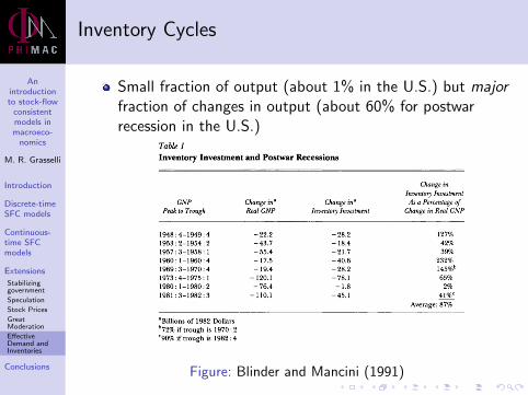
Inventory Cycles
Small fraction of output (about 1% in the U.S.) but majorfraction of changes in output (about 60% for postwarrecession in the U.S.)
Figure: Blinder and Mancini (1991)
Anintroductionto stock-flow
consistentmodels inmacroeco-
nomics
M. R. Grasselli
Introduction
Discrete-timeSFC models
Continuous-time SFCmodels
Extensions
Stabilizinggovernment
Speculation
Stock Prices
GreatModeration
EffectiveDemand andInventories
Conclusions
Notation
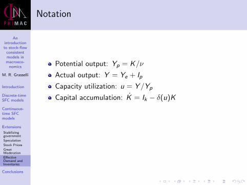
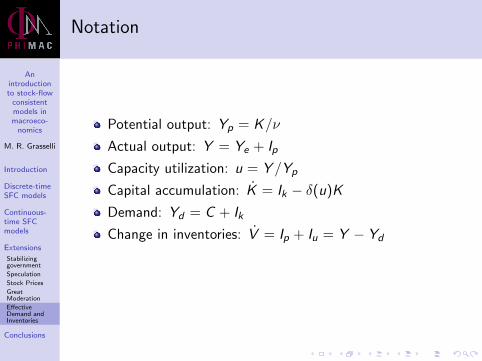
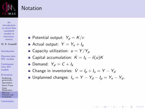
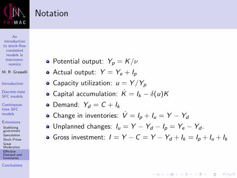
Potential output: Yp = K/ν
Actual output: Y = Ye + Ip
Capacity utilization: u = Y /Yp
Capital accumulation: K = Ik − δ(u)K
Demand: Yd = C + Ik
Change in inventories: V = Ip + Iu = Y − Yd
Unplanned changes: Iu = Y − Yd − Ip = Ye − Yd .
Gross investment: I = Y −C = Y −Yd + Ik = Ip + Iu + Ik

Anintroductionto stock-flow
consistentmodels inmacroeco-
nomics
M. R. Grasselli
Introduction
Discrete-timeSFC models
Continuous-time SFCmodels
Extensions
Stabilizinggovernment
Speculation
Stock Prices
GreatModeration
EffectiveDemand andInventories
Conclusions
Notation
Potential output: Yp = K/ν
Actual output: Y = Ye + Ip
Capacity utilization: u = Y /Yp
Capital accumulation: K = Ik − δ(u)K
Demand: Yd = C + Ik
Change in inventories: V = Ip + Iu = Y − Yd
Unplanned changes: Iu = Y − Yd − Ip = Ye − Yd .
Gross investment: I = Y −C = Y −Yd + Ik = Ip + Iu + Ik
Anintroductionto stock-flow
consistentmodels inmacroeco-
nomics
M. R. Grasselli
Introduction
Discrete-timeSFC models
Continuous-time SFCmodels
Extensions
Stabilizinggovernment
Speculation
Stock Prices
GreatModeration
EffectiveDemand andInventories
Conclusions
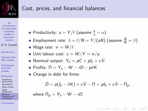
Cost, prices, and financial balances
Productivity: a = Y /` (assume aa = α)
Employment rate: λ = `/N = Y /(aN) (assume NN = β)
Wage rate: w = W /`
Unit labour cost: c = W /Y = w/a.
Nominal output: Yn = pC + pIk + cV .
Profits: Π = Yn −W − rD − pδK
Change in debt for firms:
D = p(Ik − δK ) + cV − Π = pIk + cV − Πp,
where Πp = Yn −W − rD.

Anintroductionto stock-flow
consistentmodels inmacroeco-
nomics
M. R. Grasselli
Introduction
Discrete-timeSFC models
Continuous-time SFCmodels
Extensions
Stabilizinggovernment
Speculation
Stock Prices
GreatModeration
EffectiveDemand andInventories
Conclusions
Cost, prices, and financial balances
Productivity: a = Y /` (assume aa = α)
Employment rate: λ = `/N = Y /(aN) (assume NN = β)
Wage rate: w = W /`
Unit labour cost: c = W /Y = w/a.
Nominal output: Yn = pC + pIk + cV .
Profits: Π = Yn −W − rD − pδK
Change in debt for firms:
D = p(Ik − δK ) + cV − Π = pIk + cV − Πp,
where Πp = Yn −W − rD.
Anintroductionto stock-flow
consistentmodels inmacroeco-
nomics
M. R. Grasselli
Introduction
Discrete-timeSFC models
Continuous-time SFCmodels
Extensions
Stabilizinggovernment
Speculation
Stock Prices
GreatModeration
EffectiveDemand andInventories
Conclusions
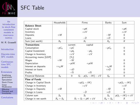
SFC Table
Households Firms Banks Sum
Balance SheetCapital stock +pK +pKInventory +cV +cVDeposits +M −M 0Loans −D +D 0
Sum (net worth) Xh Xf Xb X
Transactions current capitalConsumption −pCh +pC −pCb 0Capital Investment +pIk −pIk 0
Change in Inventory +cV −cV 0Accounting memo [GDP] [Yn]Wages +W −W 0Depreciation −pδK +pδK 0Interest on deposits +rmM −rmM 0Interest on loans −rD +rD 0Profits −Π +Π 0
Financial Balances Sh 0 Sf − p(Ik − δK )− cV Sb 0
Flow of FundsChange in Capital Stock +p(Ik − δK ) +p(Ik − δK )
Change in Inventory +cV +cV
Change in Deposits +M −M 0
Change in Loans −D +D 0
Column sum Sh Sf Sb p(Ik − δK ) + cV
Change in net worth Xh = Sh Xf = Sf + pK + cV Xb = Sb X
Anintroductionto stock-flow
consistentmodels inmacroeco-
nomics
M. R. Grasselli
Introduction
Discrete-timeSFC models
Continuous-time SFCmodels
Extensions
Stabilizinggovernment
Speculation
Stock Prices
GreatModeration
EffectiveDemand andInventories
Conclusions
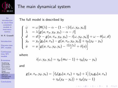
The main dynamical system
The full model is described by
ω = ω [Φ(λ)− α− (1− γ)i(ω, yd , ye)]
λ = λ [g(u, πe , yd , ye)− α− β]
d = d [r − g(u, πe , yd , ye)− i(ω, yd , ye)] + ω − θ(ω, d)ye = ye [ge(u, πe)− g(u, πe , yd , ye)] + ηe(yd − ye)
u = u[g(u, πe , yd , ye)− κ(u,πe)
ν + δ(u)]
wherei(ω, yd , ye) = ηp (mω − 1) + ηq(yd − ye)
and
g(u, πe , yd , ye) =[fd(ge(u, πe) + ηd) + 1
](yege(u, πe)
+ ηe(yd − ye))
+ ηd(yd − 1)
Anintroductionto stock-flow
consistentmodels inmacroeco-
nomics
M. R. Grasselli
Introduction
Discrete-timeSFC models
Continuous-time SFCmodels
Extensions
Stabilizinggovernment
Speculation
Stock Prices
GreatModeration
EffectiveDemand andInventories
Conclusions
Short-run dynamics
Suppose now that α + β = 0, ge(u, πe) = 0 (no growth)
Assume further that κ(u, πe) = νδ(u).
This leads to
v =[1 + fdηd ]ye − 1
ηd,
g(ye , yd) = ηe(1 + fdηd)(yd − ye) + ηd(yd − 1),
and the main system reduces toω = ω[Φ(λ)− (1− γ)i(ω, yd , ye)]
λ = λg(ye , yd)
d = d [r − g(ye , yd)− i(ω, yd , ye)] + ω − θ(ω, d)ye = −yeg(ye , yd) + ηe(yd − ye)u = ug(ye , yd)
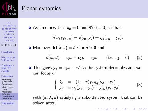
Anintroductionto stock-flow
consistentmodels inmacroeco-
nomics
M. R. Grasselli
Introduction
Discrete-timeSFC models
Continuous-time SFCmodels
Extensions
Stabilizinggovernment
Speculation
Stock Prices
GreatModeration
EffectiveDemand andInventories
Conclusions
Planar dynamics
Assume now that ηp = 0 and Φ(·) ≡ 0, so that
i(ω, yd , ye) = i(yd , ye) = ηq(yd − ye).
Moreover, let δ(u) = δu for δ > 0 and
θ(ω, d) = c1ω + c2d = c1ω (i.e. c2 = 0) (2)
This gives yd = c1ω + νδ so the system decouples and wecan focus on{
yd = −(1− γ)ydηq(yd − ye)ye = ηe(yd − ye)− yeg(ye , yd)
(3)
with (ω, λ, d) satisfying a subordinated system that can besolved after.
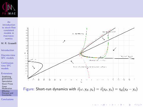
Anintroductionto stock-flow
consistentmodels inmacroeco-
nomics
M. R. Grasselli
Introduction
Discrete-timeSFC models
Continuous-time SFCmodels
Extensions
Stabilizinggovernment
Speculation
Stock Prices
GreatModeration
EffectiveDemand andInventories
Conclusions
Figure: Short-run dynamics with i(ω, yd , ye) = i(yd , ye) = ηq(yd − ye)

Anintroductionto stock-flow
consistentmodels inmacroeco-
nomics
M. R. Grasselli
Introduction
Discrete-timeSFC models
Continuous-time SFCmodels
Extensions
Stabilizinggovernment
Speculation
Stock Prices
GreatModeration
EffectiveDemand andInventories
Conclusions
Other work
Heterogeneous agents and mean-field aggregation -Grasselli and Li (2018a) and (2018b)
Two classes of households and inequality - Giraud andGrasselli (2019)
Monetary policy, negative interest rates, digital currencies- Grasselli and Lipton (2019a)
Narrow banking - Grasselli and Lipton (2019b)
Banking networks and macroeconomics - Grasselli andLipton
Climate change economics - Bolker, Grasselli, Holmes,Presta
Anintroductionto stock-flow
consistentmodels inmacroeco-
nomics
M. R. Grasselli
Introduction
Discrete-timeSFC models
Continuous-time SFCmodels
Extensions
Conclusions
Concluding thoughts
Solow (1990): The true test of a simple model is whetherit helps us to make sense of the world. Marx was, ofcourse, dead wrong about this. We have changed theworld in all sorts of ways, with mixed results; the point isto interpret it.
Schumpeter (1939): Cycles are not, like tonsils, separablethings that might be treated by themselves, but are, likethe beat of the heart, of the essence of the organism thatdisplays them.
Anintroductionto stock-flow
consistentmodels inmacroeco-
nomics
M. R. Grasselli
Introduction
Discrete-timeSFC models
Continuous-time SFCmodels
Extensions
Conclusions
Concluding thoughts (continued)
Since Keynes’s death it has developed in two radicallydifferent approaches:
1 The dominant one has the appearance of mathematicalrigour (the SMD theorems notwithstanding), but is basedon implausible assumptions, has poor fit to data in general,and is disastrously wrong during crises. Finance plays anegligible role
2 The heterodox approach is grounded in history andinstitutional understanding, takes empirical work muchmore seriously, but is generally averse to mathematics.Finance plays a major role.
Stock-flow consistent agent-based models, complementedby mean-field approximations and other techniques(including mean-field games), have the potential toredefine the role of mathematics in macroeconomics.
Thank you!