1

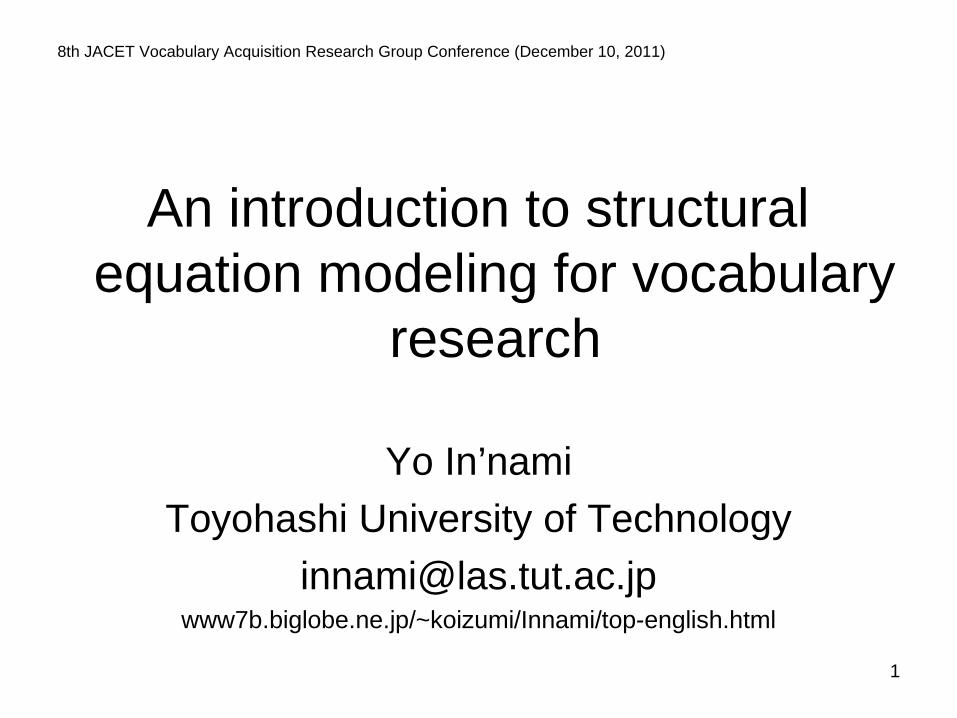
8th JACET Vocabulary Acquisition Research Group Conference (December 10, 2011)

An introduction to structural equation modeling for vocabulary

research

Yo In’nami

Toyohashi University of Technology

innami@las.tut.ac.jpwww7b.biglobe.ne.jp/~koizumi/Innami/top-english.html

2

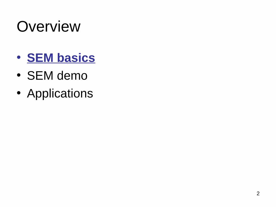
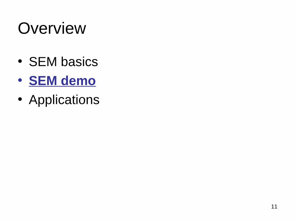
Overview

• SEM basics

• SEM demo

• Applications

3

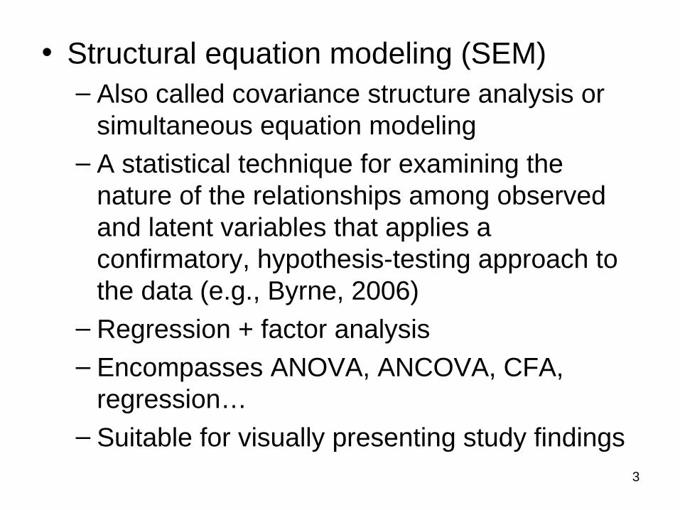
• Structural equation modeling (SEM)– Also called covariance structure analysis or

simultaneous equation modeling– A statistical technique for examining the

nature of the relationships among observed and latent variables that applies a confirmatory, hypothesis-testing approach to the data (e.g., Byrne, 2006)

– Regression + factor analysis– Encompasses ANOVA, ANCOVA, CFA,

regression…– Suitable for visually presenting study findings

4

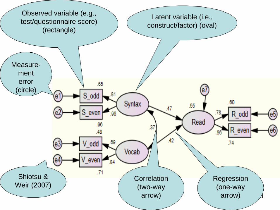
Observed variable (e.g., test/questionnaire score)

(rectangle)

Measure-ment error

(circle)

Latent variable (i.e., construct/factor) (oval)

Correlation (two-way

arrow)

Regression (one-way

arrow)

Shiotsu & Weir (2007)

5

The diagram was displayed at the workshop.

Tseng, Dörnyel, & Schmitt (2006,

p. 93)

6

The diagram was displayed at the workshop.

Mizumoto & Takeuchi (in

press)

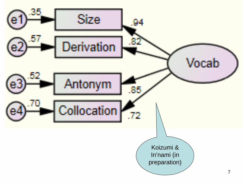
7

Koizumi & In’nami (in

preparation)

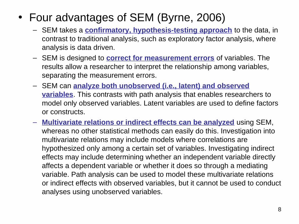
• Four advantages of SEM (Byrne, 2006)

– SEM takes a confirmatory, hypothesis-testing approach to the data, in contrast to traditional analysis, such as exploratory factor analysis, where analysis is data driven.

– SEM is designed to correct for measurement errors of variables. The results allow a researcher to interpret the relationship among variables, separating the measurement errors.

– SEM can analyze both unobserved (i.e., latent) and observed variables. This contrasts with path analysis that enables researchers to model only observed variables. Latent variables are used to define factors or constructs.

– Multivariate relations or indirect effects can be analyzed using SEM, whereas no other statistical methods can easily do this. Investigation into multivariate relations may include models where correlations are hypothesized only among a certain set of variables. Investigating indirect effects may include determining whether an independent variable directly affects a dependent variable or whether it does so through a mediating variable. Path analysis can be used to model these multivariate relations or indirect effects with observed variables, but it cannot be used to conduct analyses using unobserved variables.

8

9

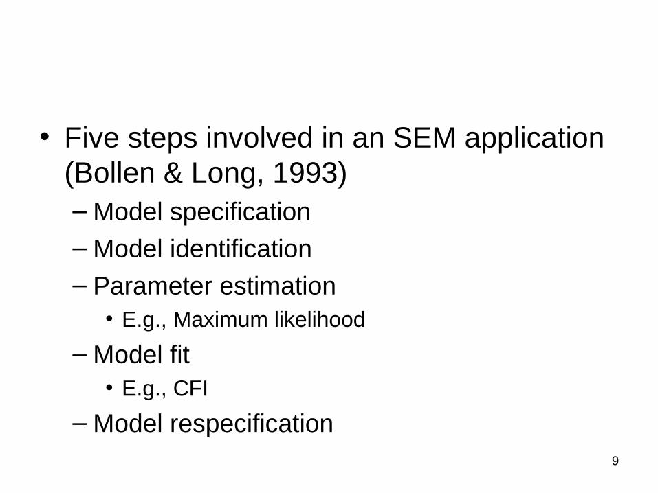
• Five steps involved in an SEM application (Bollen & Long, 1993)– Model specification– Model identification– Parameter estimation

• E.g., Maximum likelihood

– Model fit• E.g., CFI

– Model respecification

10

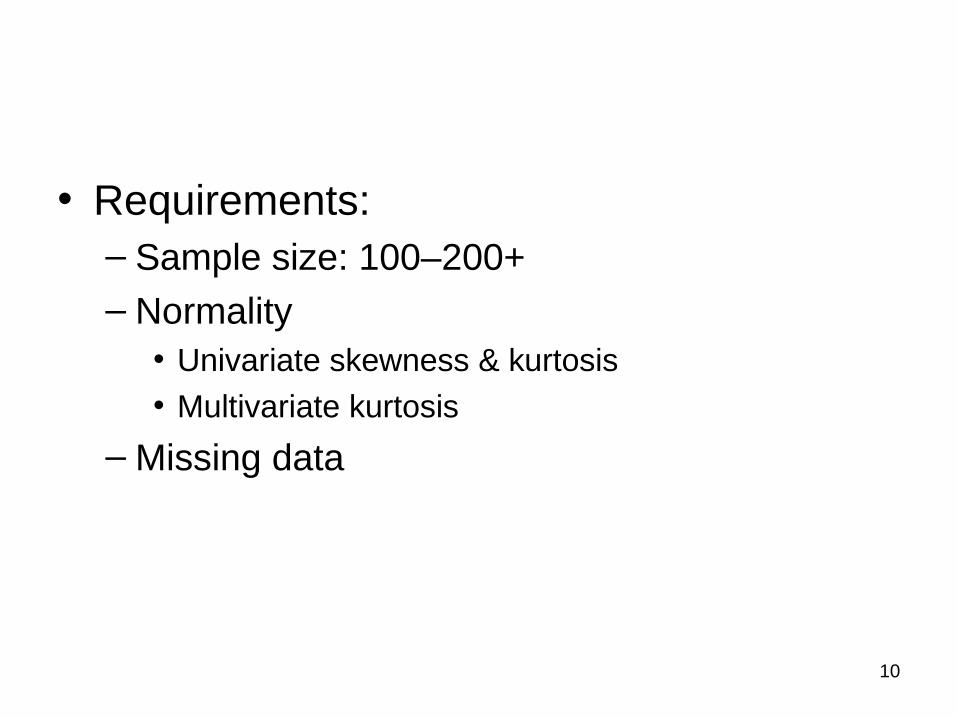
• Requirements:– Sample size: 100–200+– Normality

• Univariate skewness & kurtosis• Multivariate kurtosis

– Missing data

11

Overview

• SEM basics

• SEM demo

• Applications

12

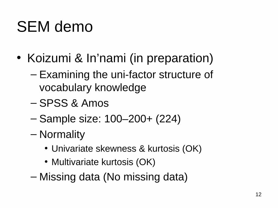
SEM demo

• Koizumi & In’nami (in preparation)– Examining the uni-factor structure of

vocabulary knowledge– SPSS & Amos– Sample size: 100–200+ (224)– Normality

• Univariate skewness & kurtosis (OK)

• Multivariate kurtosis (OK)

– Missing data (No missing data)

13

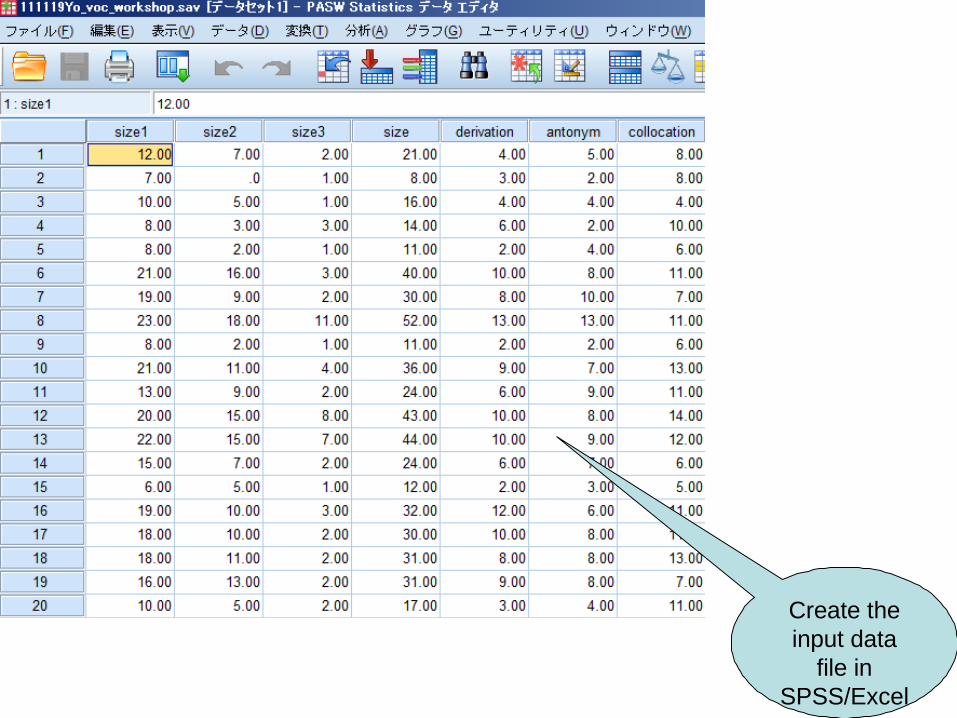
Create the input data

file in SPSS/Excel

14

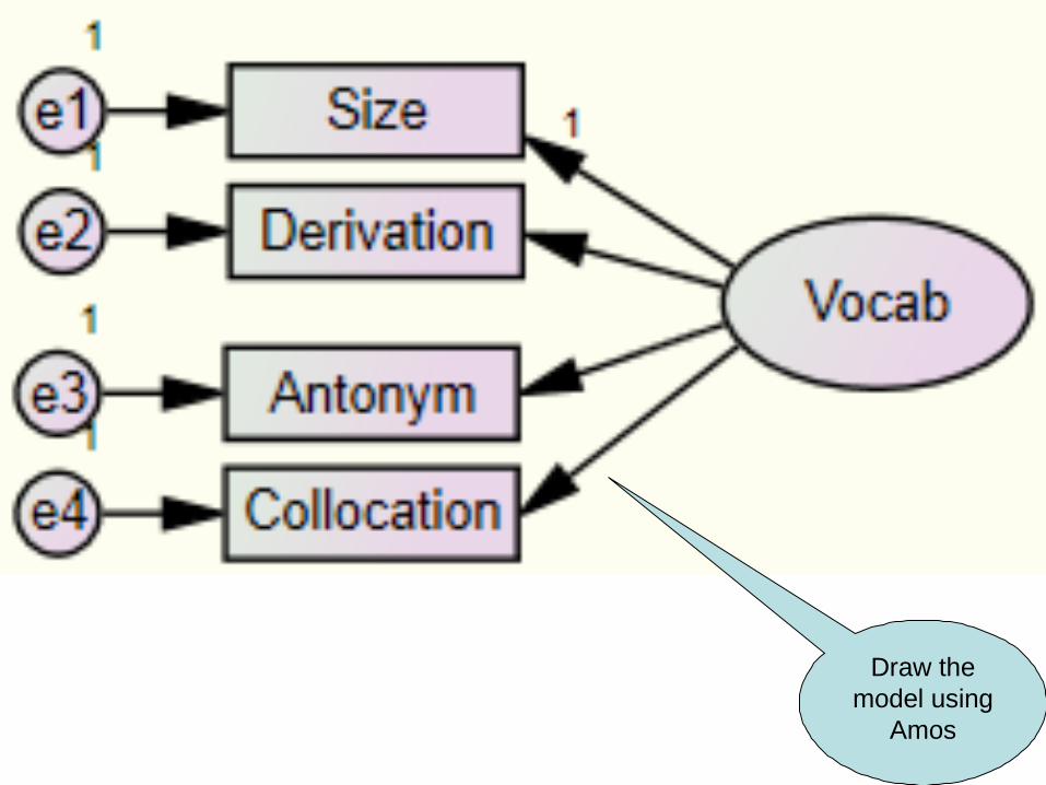
Draw the model using

Amos

15

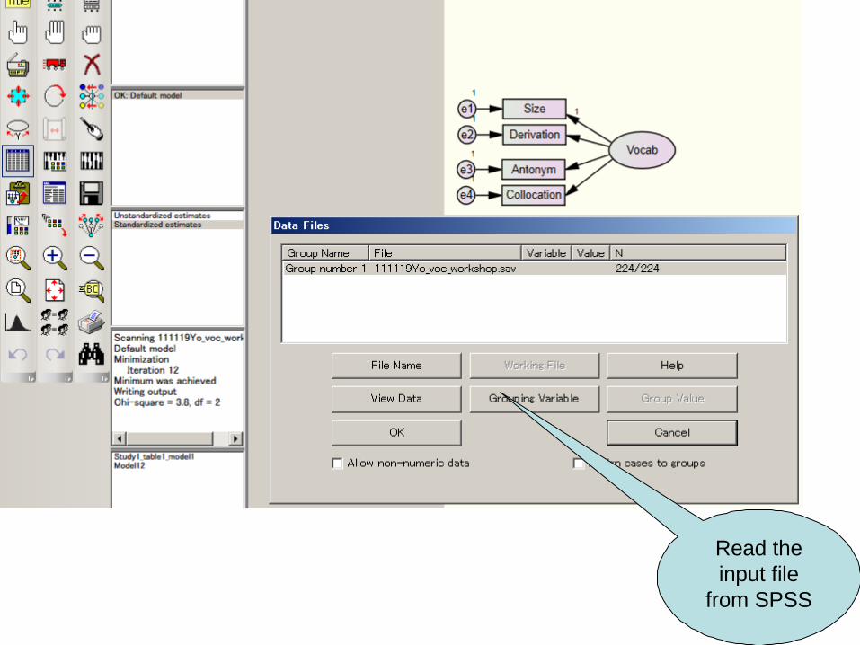
Read the input file

from SPSS

16

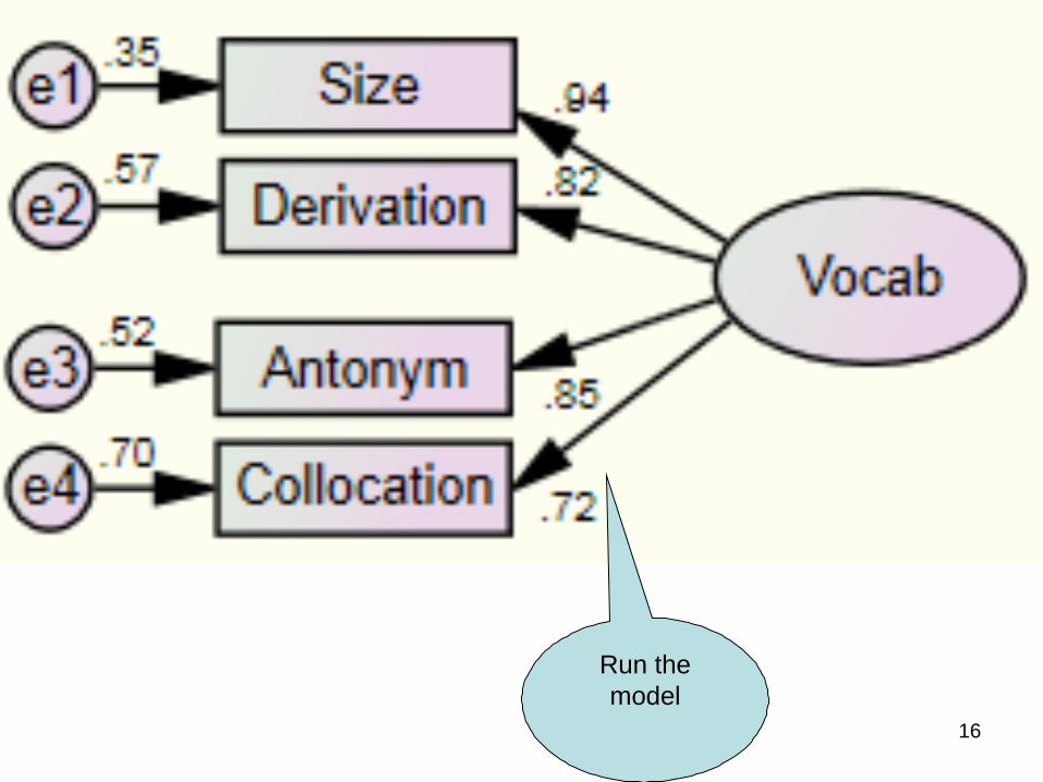
Run the model

17

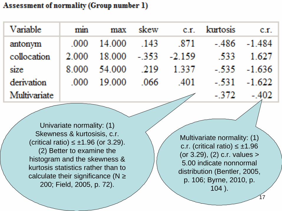
Univariate normality: (1) Skewness & kurtosisis, c.r.

(critical ratio) ≤ ±1.96 (or 3.29). (2) Better to examine the

histogram and the skewness & kurtosis statistics rather than to calculate their significance (N ≥

200; Field, 2005, p. 72).

Multivariate normality: (1) c.r. (critical ratio) ≤ ±1.96 (or 3.29), (2) c.r. values > 5.00 indicate nonnormal

distribution (Bentler, 2005, p. 106; Byrne, 2010, p.

104 ).

18

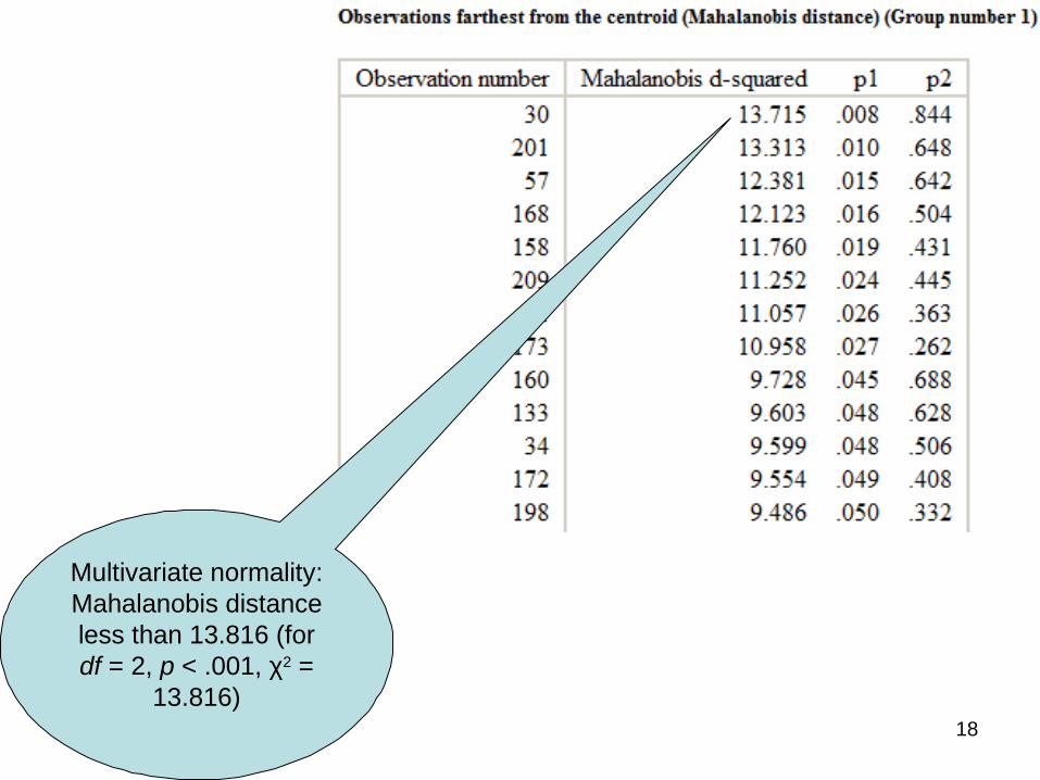
Multivariate normality: Mahalanobis distance less than 13.816 (for df = 2, p < .001, χ2 =

13.816)

19

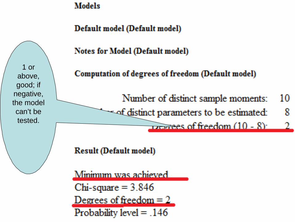
1 or above, good; if

negative, the model can’t be tested.

20

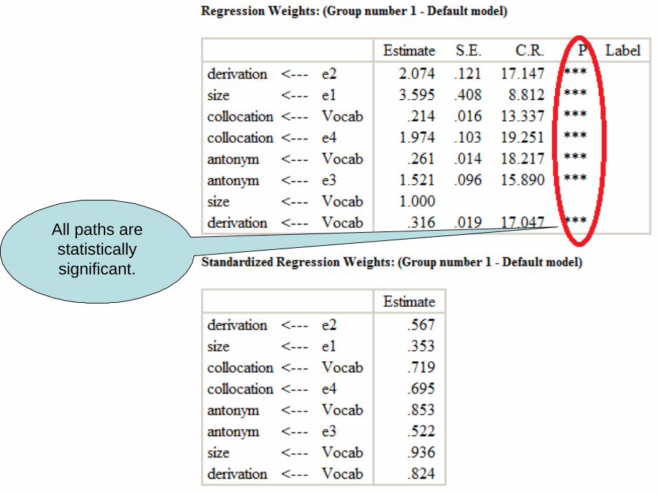
All paths are statistically significant.

21

22

23

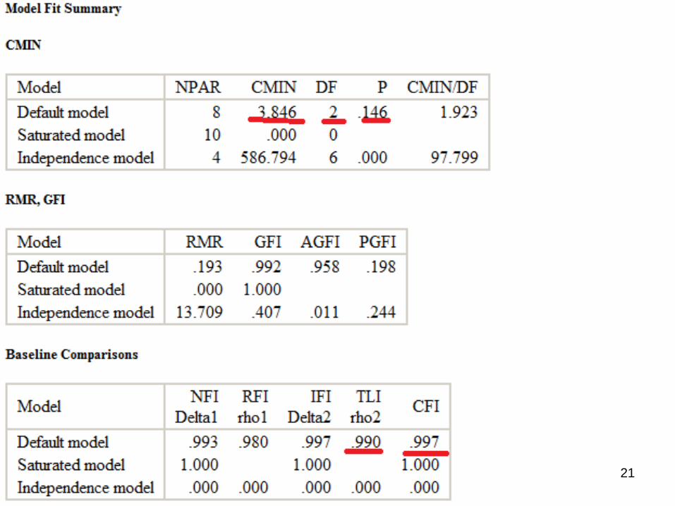
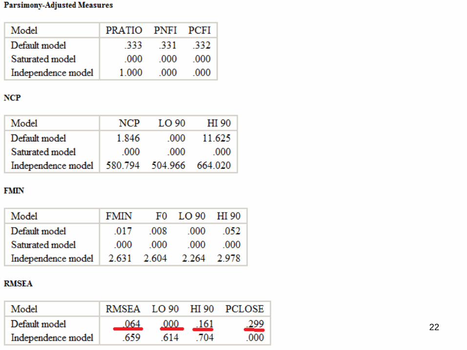
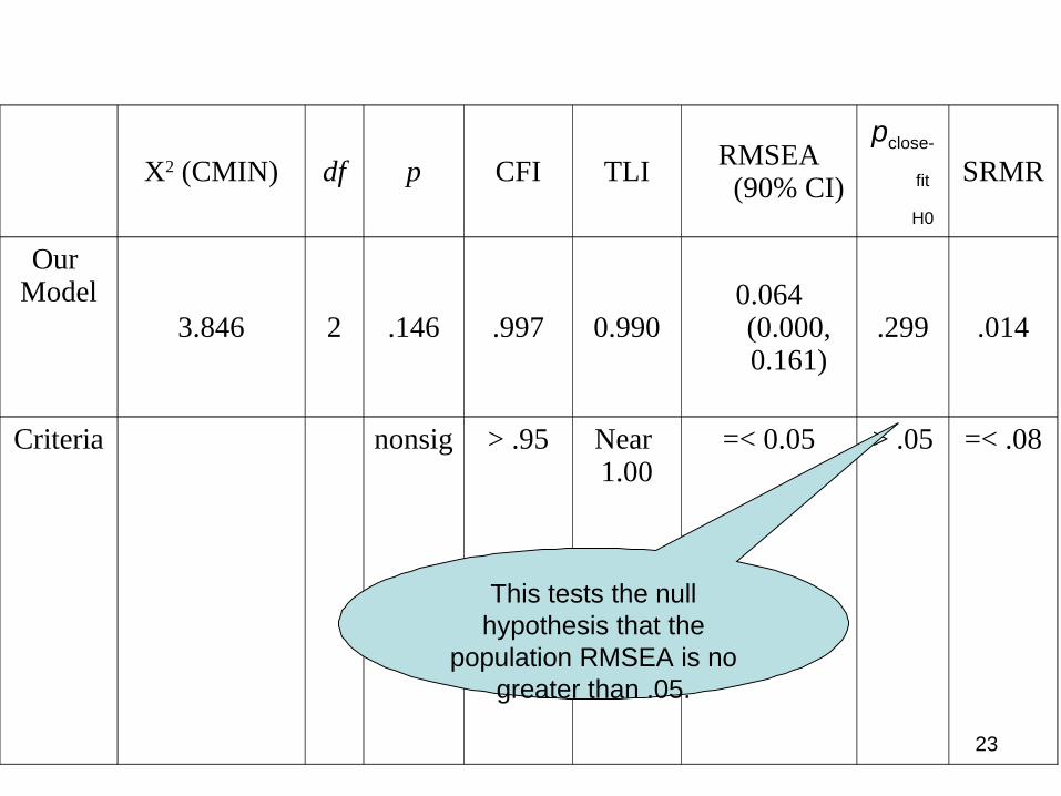
Χ2 (CMIN) df p CFI TLIRMSEA

(90% CI)

pclose-

fit

H0

SRMR

Our Model

3.846 2 .146 .997 0.9900.064 (0.000, 0.161)

.299 .014

Criteria nonsig > .95 Near 1.00

=< 0.05 > .05 =< .08

This tests the null hypothesis that the

population RMSEA is no greater than .05.

24

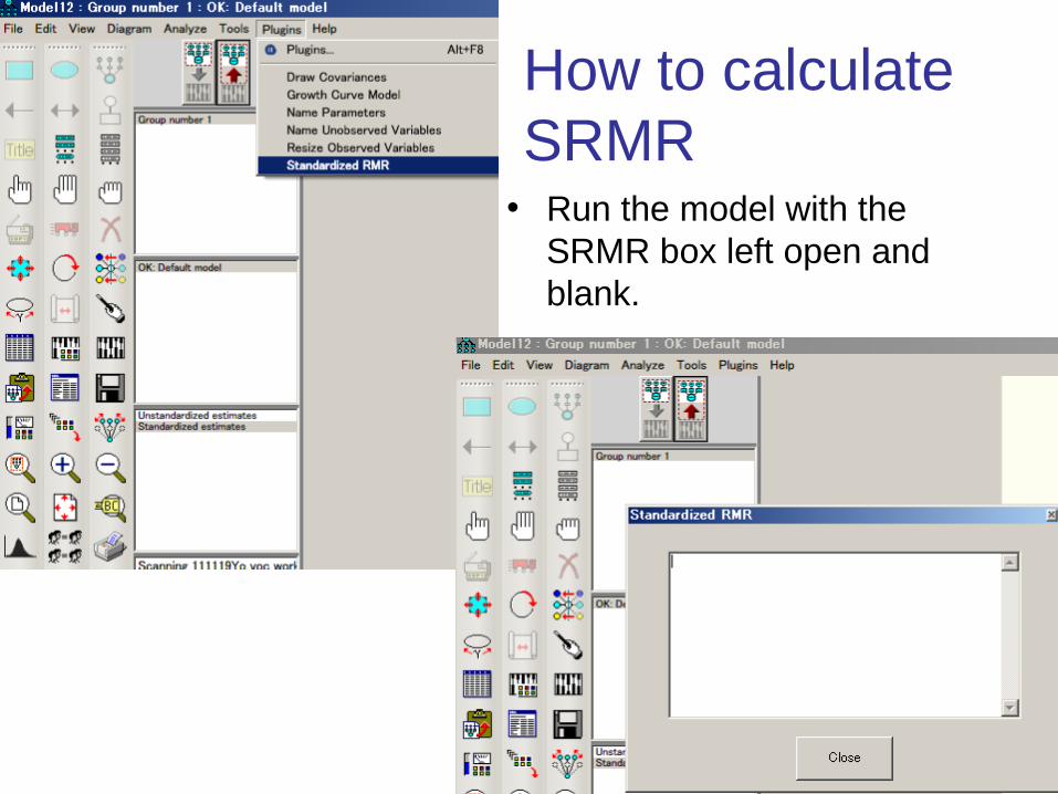
How to calculate SRMR

• Run the model with the SRMR box left open and blank.

25

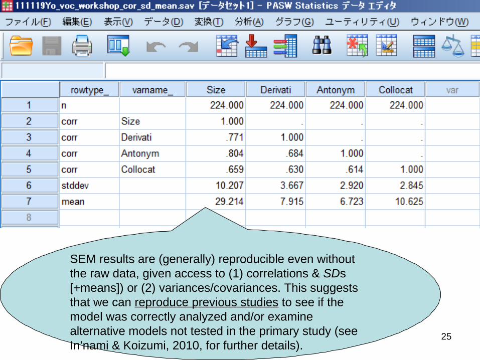
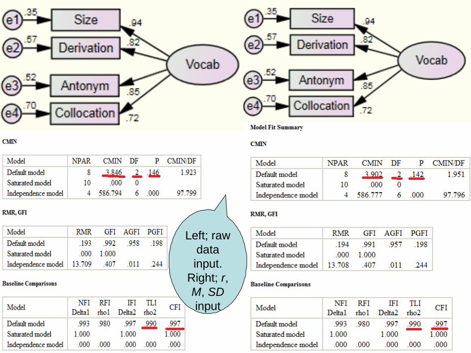
SEM results are (generally) reproducible even without the raw data, given access to (1) correlations & SDs [+means]) or (2) variances/covariances. This suggests that we can reproduce previous studies to see if the model was correctly analyzed and/or examine alternative models not tested in the primary study (see In’nami & Koizumi, 2010, for further details).

26

27

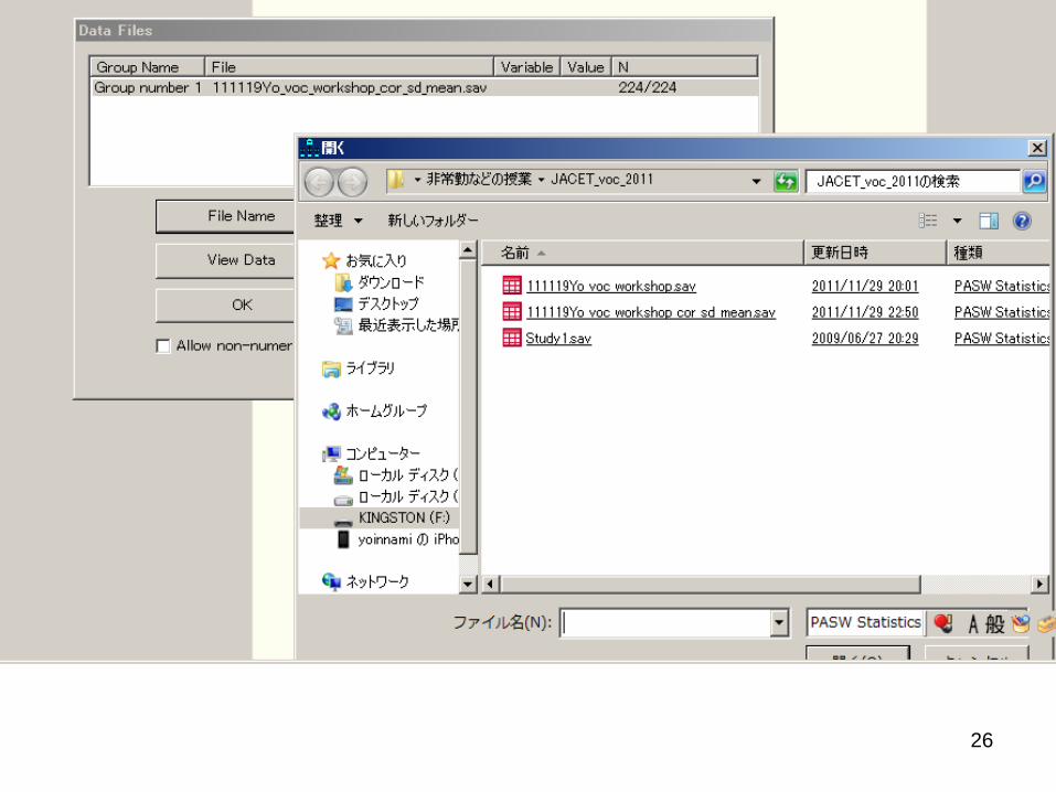
Left; raw data input.

Right; r, M, SD input

28

Overview

• SEM basics

• SEM demo

• Applications

29

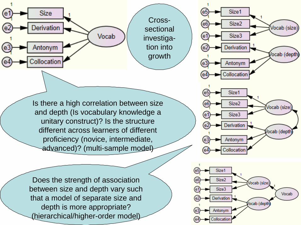
Is there a high correlation between size and depth (Is vocabulary knowledge a

unitary construct)? Is the structure different across learners of different

proficiency (novice, intermediate, advanced)? (multi-sample model)

Does the strength of association between size and depth vary such that a model of separate size and

depth is more appropriate? (hierarchical/higher-order model)

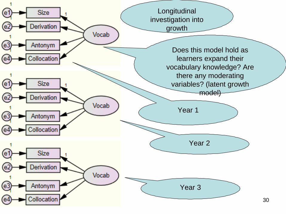
Cross-sectional investiga-tion into growth

30

Year 3

Year 1

Year 2

Does this model hold as learners expand their

vocabulary knowledge? Are there any moderating

variables? (latent growth model)

Longitudinal investigation into

growth

31

• The diagram was displayed at the workshop.

Tseng & Schmitt, (2008)

32

• The diagram was displayed at the workshop.

Tremblay & Gardner (1995)

33

• The diagram was displayed at the workshop.

Yashima (2002)

34

• The diagram was displayed at the workshop.

Matsumura (2003); latent growth model

35

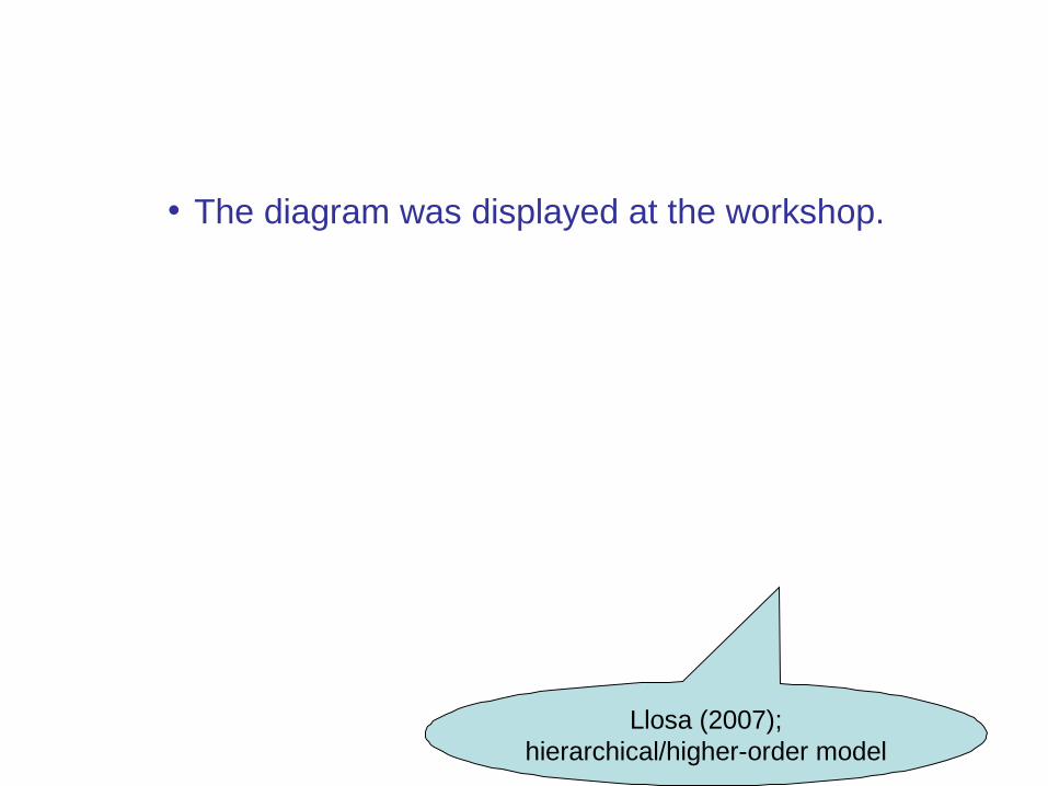
• The diagram was displayed at the workshop.

Llosa (2007); hierarchical/higher-order model

36

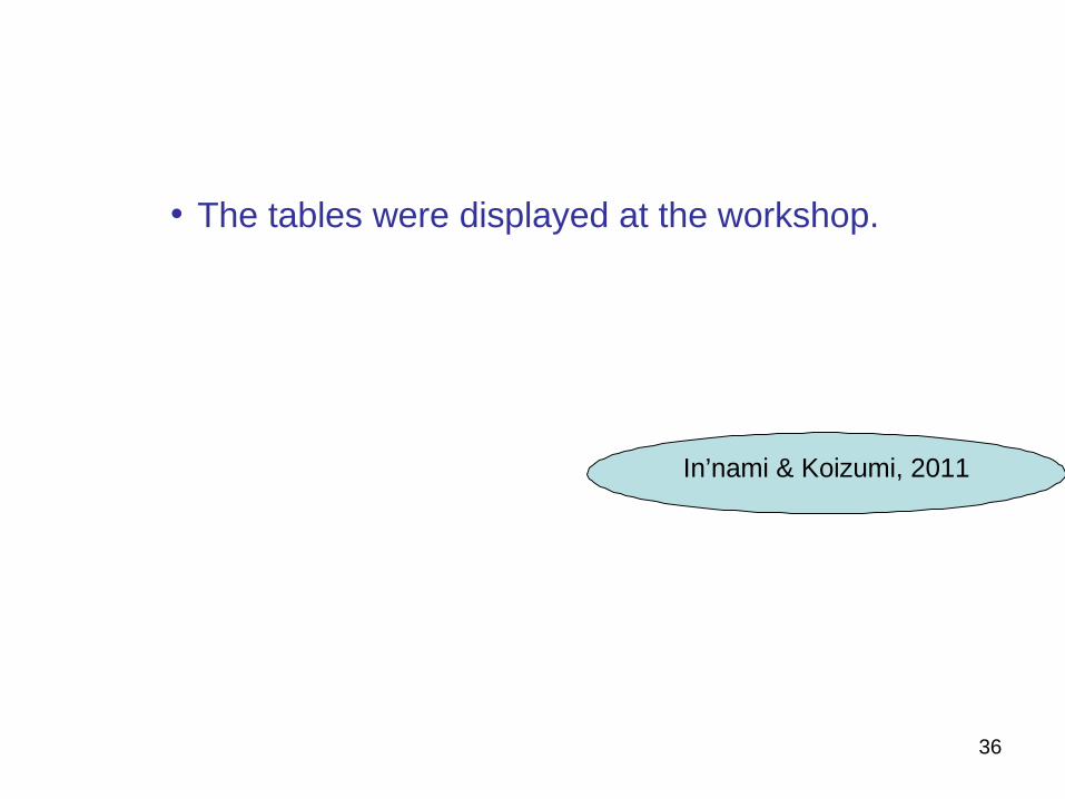
• The tables were displayed at the workshop.

In’nami & Koizumi, 2011

37

• The table was displayed at the workshop.

38

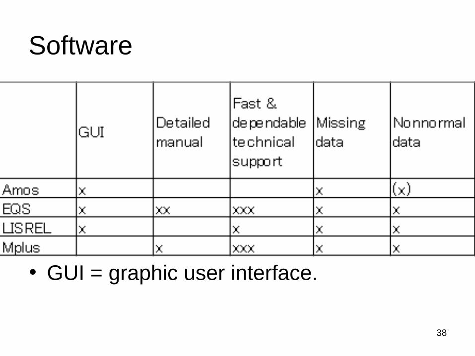
Software

• GUI = graphic user interface.

39

SEMNET

• http://www2.gsu.edu/~mkteer/semnet.html

40

References

• Bentler, P. M. (2005). EQS 6 structural equations program manual. Encino, CA: Multivariate Software.

• Bollen, K. A., & Long, J. S. (1993). Introduction. In K. A. Bollen & J. S. Long (Eds.), Testing structural equation models (pp. 1–9). Newbury Park, CA: Sage.

• Brown, T. A. (2006). Confirmatory factor analysis for applied research. New York: Guilford.

• Byrne, B. M. (2010). Structural equation modeling with AMOS: Basic concepts, applications, and programming (2nd ed.). Mahwah, NJ: Erlbaum.

• Byrne, B. M. (2006). Structural equation modeling with EQS: Basic concepts, applications, and programming (2nd ed.). Mahwah, NJ: Erlbaum.

• Byrne, B. M. (2011). Structural equation modeling with Mplus: Basic concepts, applications, and programming. Mahwah, NJ: Erlbaum.

• Field, A. (2005). Discovering statistics using SPSS (2nd ed.). London: Sage.• In’nami, Y., & Koizumi, R. (2010). Can structural equation models in second language

testing and learning research be successfully replicated? International Journal of Testing, 10, 262–273.

• In’nami, Y., & Koizumi, R. (2011). Structural equation modeling in language testing and learning research: A review. Language Assessment Quarterly, 8, 250–276.

41

References

• Kline, R. B. (2011). Principles and practice of structural equation modeling (3rd ed.). New York: Guilford.

• Koizumi, R., & In’nami, Y. (in preparation).• Llosa, L. (2007). Validating a standards-based classroom assessment of English proficiency: A

multitrait-multimethod approach. Language Testing, 24, 489–515.• Matsumura, S. (2003). Modelling the relationships among interlanguage pragmatic development,

L2 proficiency, and exposure to L2. Applied Linguistics, 24, 465–491.• Mizumoto, A., & Takeuchi, O. (in press). Adaptation and validation of self-regulating capacity in

vocabulary learning scale. Applied Linguistics.• Shiotsu, T., & Weir, C. J. (2007). The relative significance of syntactic knowledge and vocabulary

breadth in the prediction of reading comprehension test performance. Language Testing, 24, 99–128.

• Tremblay, P. F., & Gardner, R. C. (1995). Expanding the motivation construct in language learning. Modern Language Journal, 79, 505–518.

• Tseng, W.-T., Dornyei, Z., & Schmitt, N. (2006). A new approach to assessing strategic learning: The case of self-regulation in vocabulary acquisition. Applied Linguistics, 27, 78–102.

• Tseng, W.-T., & Schmitt, N. (2008). Toward a model of motivated vocabulary learning: A structural equation modeling approach. Language Learning, 58, 357–400.

• Yashima, T. (2002). Willingness to communicate in a second language: The Japanese EFL context. Modern Language Journal, 86, 54–66.