Embed Size (px)
Citation preview
An Introduction to Vectors, Vector Operators and Vector Analysis
Conceived as s a supplementary text and reference book for undergraduate and graduatestudents of science and engineering, this book intends communicating the fundamentalconcepts of vectors and their applications. It is divided into three units. The first unit dealswith basic formulation: both conceptual and theoretical. It discusses applications ofalgebraic operations, Levi-Civita notation and curvilinear coordinate systems likespherical polar and parabolic systems. Structures and analytical geometry of curves andsurfaces is covered in detail.
The second unit discusses algebra of operators and their types. It explains the equivalencebetween the algebra of vector operators and the algebra of matrices. Formulation ofeigenvectors and eigenvalues of a linear vector operator are discussed using vector algebra.Topics including Mohr’s algorithm, Hamilton’s theorem and Euler’s theorem are discussedin detail. The unit ends with a discussion on transformation groups, rotation group, groupof isometries and the Euclidean group, with applications to rigid displacements.
The third unit deals with vector analysis. It discusses important topics including vectorvalued functions of a scalar variable, functions of vector argument (both scalar valued andvector valued): thus covering both the scalar and vector fields and vector integration
Pramod S. Joag is presently working as CSIR Emeritus Scientist at the Savitribai PhuleUniversity of Pune, India. For over 30 years he has been teaching classical mechanics,quantum mechanics, electrodynamics, solid state physics, thermodynamics and statisticalmechanics at undergraduate and graduate levels. His research interests include quantuminformation, and more specifically measures of quantum entanglement and quantumdiscord, production of multipartite entangled states, entangled Fermion systems, modelsof quantum nonlocality etc.

An Introduction to Vectors, VectorOperators and Vector Analysis
Pramod S. Joag
4843/24, 2nd Floor, Ansari Road, Daryaganj, Delhi - 110002, India
Cambridge University Press is part of the University of Cambridge.
It furthers the University’s mission by disseminating knowledge in the pursuit ofeducation, learning and research at the highest international levels of excellence.
www.cambridge.orgInformation on this title: www.cambridge.org/9781107154438
© Pramod S. Joag 2016
This publication is in copyright. Subject to statutory exceptionand to the provisions of relevant collective licensing agreements,no reproduction of any part may take place without the writtenpermission of Cambridge University Press.
First published 2016
Printed in India
A catalogue record for this publication is available from the British LibraryLibrary of Congress Cataloging-in-Publication DataNames: Joag, Pramod S., 1951- author.Title: An introduction to vectors, vector operators and vector analysis /
Pramod S. Joag.Description: Daryaganj, Delhi, India : Cambridge University Press, 2016. |
Includes bibliographical references and index.Identifiers: LCCN 2016019490| ISBN 9781107154438 (hardback) | ISBN 110715443X
(hardback)Subjects: LCSH: Vector analysis. |Mathematical physics.Classification:LCC QC20.7.V4 J63 2016 | DDC 512/.5–dc23 LC record available athttps://lccn.loc.gov/2016019490
ISBN 978-1-107-15443-8 Hardback
Cambridge University Press has no responsibility for the persistence or accuracyof URLs for external or third-party internet websites referred to in this publication,and does not guarantee that any content on such websites is, or will remain,accurate or appropriate.

To Ela and Ninadwho made me write this document

Contents
Figures xiiiTables xxPreface xxiNomenclature xxv
I Basic Formulation
1 Getting Concepts and Gathering Tools 3
1.1 Vectors and Scalars 31.2 Space and Direction 41.3 Representing Vectors in Space 61.4 Addition and its Properties 8
1.4.1 Decomposition and resolution of vectors 131.4.2 Examples of vector addition 16
1.5 Coordinate Systems 181.5.1 Right-handed (dextral) and left-handed coordinate systems 18
1.6 Linear Independence, Basis 191.7 Scalar and Vector Products 22
1.7.1 Scalar product 221.7.2 Physical applications of the scalar product 301.7.3 Vector product 321.7.4 Generalizing the geometric interpretation of the vector product 361.7.5 Physical applications of the vector product 38
1.8 Products of Three or More Vectors 391.8.1 The scalar triple product 391.8.2 Physical applications of the scalar triple product 431.8.3 The vector triple product 45
1.9 Homomorphism and Isomorphism 45
viii Contents
1.10 Isomorphism with R3 451.11 A New Notation: Levi-Civita Symbols 481.12 Vector Identities 521.13 Vector Equations 541.14 Coordinate Systems Revisited: Curvilinear Coordinates 57
1.14.1 Spherical polar coordinates 571.14.2 Parabolic coordinates 60
1.15 Vector Fields 671.16 Orientation of a Triplet of Non-coplanar Vectors 68
1.16.1 Orientation of a plane 72
2 Vectors and Analytic Geometry 74
2.1 Straight Lines 742.2 Planes 832.3 Spheres 892.4 Conic Sections 90
3 Planar Vectors and Complex Numbers 94
3.1 Planar Curves on the Complex Plane 943.2 Comparison of Angles Between Vectors 993.3 Anharmonic Ratio: Parametric Equation to a Circle 1003.4 Conformal Transforms, Inversion 1013.5 Circle: Constant Angle and Constant Power Theorems 1033.6 General Circle Formula 1053.7 Circuit Impedance and Admittance 1063.8 The Circle Transformation 107
II Vector Operators
4 Linear Operators 115
4.1 Linear Operators on E3 1154.1.1 Adjoint operators 1174.1.2 Inverse of an operator 1174.1.3 Determinant of an invertible linear operator 1194.1.4 Non-singular operators 1214.1.5 Examples 121
4.2 Frames and Reciprocal Frames 1244.3 Symmetric and Skewsymmetric Operators 126
4.3.1 Vector product as a skewsymmetric operator 128
Contents ix
4.4 Linear Operators and Matrices 1294.5 An Equivalence Between Algebras 1304.6 Change of Basis 132
5 Eigenvalues and Eigenvectors 134
5.1 Eigenvalues and Eigenvectors of a Linear Operator 1345.1.1 Examples 138
5.2 Spectrum of a Symmetric Operator 1415.3 Mohr’s Algorithm 147
5.3.1 Examples 1515.4 Spectrum of a 2× 2 Symmetric Matrix 1555.5 Spectrum of Sn 156
6 Rotations and Reflections 158
6.1 Orthogonal Transformations: Rotations and Reflections 1586.1.1 The canonical form of the orthogonal operator for reflection 1616.1.2 Hamilton’s theorem 164
6.2 Canonical Form for Linear Operators 1656.2.1 Examples 168
6.3 Rotations 1706.3.1 Matrices representing rotations 176
6.4 Active and Passive Transformations: Symmetries 1806.5 Euler Angles 1846.6 Euler’s Theorem 188
7 Transformation Groups 191
7.1 Definition and Examples 1917.2 The Rotation Group O +(3) 1967.3 The Group of Isometries and the Euclidean Group 199
7.3.1 Chasles theorem 2047.4 Similarities and Collineations 205
III Vector Analysis
8 Preliminaries 215
8.1 Fundamental Notions 2158.2 Sets and Mappings 2168.3 Convergence of a Sequence 2178.4 Continuous Functions 220
x Contents
9 Vector Valued Functions of a Scalar Variable 221
9.1 Continuity and Differentiation 2219.2 Geometry and Kinematics: Space Curves and Frenet–Seret Formulae 225
9.2.1 Normal, rectifying and osculating planes 2369.2.2 Order of contact 2389.2.3 The osculating circle 2399.2.4 Natural equations of a space curve 2409.2.5 Evolutes and involutes 243
9.3 Plane Curves 2489.3.1 Three different parameterizations of an ellipse 2489.3.2 Cycloids, epicycloids and trochoids 2539.3.3 Orientation of curves 258
9.4 Chain Rule 2639.5 Scalar Integration 2639.6 Taylor Series 264
10 Functions with Vector Arguments 266
10.1 Need for the Directional Derivative 26610.2 Partial Derivatives 26610.3 Chain Rule 26910.4 Directional Derivative and the Grad Operator 27110.5 Taylor series 27810.6 The Differential 27910.7 Variation on a Curve 28110.8 Gradient of a Potential 28210.9 Inverse Maps and Implicit Functions 283
10.9.1 Inverse mapping theorem 28410.9.2 Implicit function theorem 28510.9.3 Algorithm to construct the inverse of a map 287
10.10 Differentiating Inverse Functions 29110.11 Jacobian for the Composition of Maps 29410.12 Surfaces 29710.13 The Divergence and the Curl of a Vector Field 30410.14 Differential Operators in Curvilinear Coordinates 313
11 Vector Integration 323
11.1 Line Integrals and Potential Functions 32311.1.1 Curl of a vector field and the line integral 341
Contents xi
11.2 Applications of the Potential Functions 34411.3 Area Integral 35711.4 Multiple Integrals 360
11.4.1 Area of a planar region: Jordan measure 36111.4.2 Double integral 36311.4.3 Integral estimates 36911.4.4 Triple integrals 37111.4.5 Multiple integrals as successive single integrals 37211.4.6 Changing variables of integration 37811.4.7 Geometrical applications 38211.4.8 Physical applications of multiple integrals 390
11.5 Integral Theorems of Gauss and Stokes in Two-dimensions 39511.5.1 Integration by parts in two dimensions: Green’s theorem 400
11.6 Applications to Two-dimensional Flows 40211.7 Orientation of a Surface 40611.8 Surface Integrals 414
11.8.1 Divergence of a vector field and the surface integral 41911.9 Diveregence Theorem in Three-dimensions 421
11.10 Applications of the Gauss’s Theorem 42311.10.1 Exercises on the divergence theorem 427
11.11 Integration by Parts and Green’s Theorem in Three-dimensions 42911.11.1 Transformation of ∆U to spherical coordinates 430
11.12 Helmoltz Theorem 43211.13 Stokes Theorem in Three-dimensions 434
11.13.1 Physical interpretation of Stokes theorem 43611.13.2 Exercises on Stoke’s theorem 437
12 Odds and Ends 444
12.1 Rotational Velocity of a Rigid Body 44412.2 3-D Harmonic Oscillator 449
12.2.1 Anisotropic oscillator 45412.3 Projectiles and Terestrial Effects 456
12.3.1 Optimum initial conditions for netting a basket ball 45612.3.2 Optimum angle of striking a golf ball 45912.3.3 Effects of Coriolis force on a projectile 462
12.4 Satellites and Orbits 46812.4.1 Geometry and dynamics: Circular motion 46812.4.2 Hodograph of an orbit 470
xii Contents
12.4.3 Orbit after an impulse 47312.5 A charged Particle in Uniform Electric and Magnetic Fields 475
12.5.1 Uniform magnetic field 47512.5.2 Uniform electric and magnetic fields 478
12.6 Two-dimensional Steady and Irrotational Flow of an Incompressible Fluid 483
Appendices
A Matrices and Determinants 489A.1 Matrices and Operations on them 489A.2 Square Matrices, Inverse of a Matrix, Orthogonal Matrices 494A.3 Linear and Multilinear Forms of Vectors 497A.4 Alternating Multilinear Forms: Determinants 499A.5 Principal Properties of Determinants 502
A.5.1 Determinants and systems of linear equations 505A.5.2 Geometrical interpretation of determinants 506
B Dirac Delta Function 510
Bibliography 515Index 517
Figures
1.1 (a) A line indicates two possible directions. A line with an arrow specifiesa unique direction. (b) The angle between two directions is the amount bywhich one line is to be rotated so as to coincide with the other along withthe arrows. Note the counterclockwise and clockwise rotations. (c) The anglebetween two directions is measured by the arc of the unit circle swept by therotating direction. 5
1.2 We can choose the angle between directions≤ π by choosing which directionis to be rotated (counterclockwise) towards which. 5
1.3 Different representations of the same vector in space 71.4 Shifting origin makes (a) two different vectors correspond to the same point
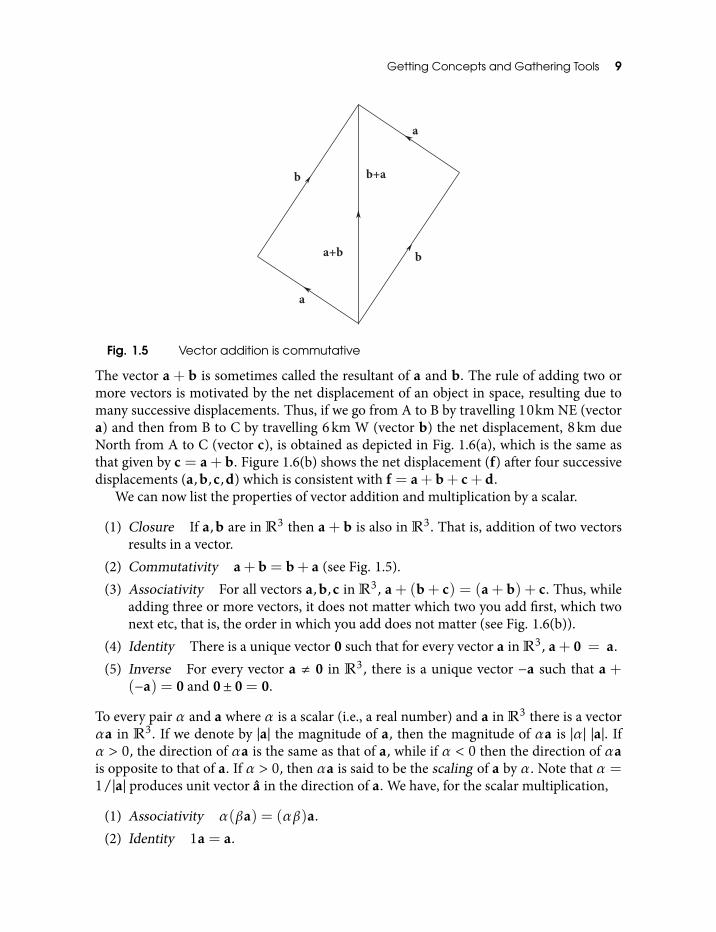
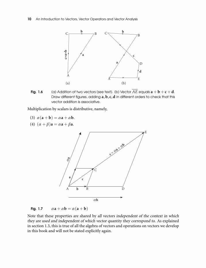
and (b) two different points correspond to the same vector 81.5 Vector addition is commutative 91.6 (a) Addition of two vectors (see text). (b) Vector AE equals a + b + c + d.
Draw different figures, adding a,b,c,d in different orders to check that thisvector addition is associative. 10
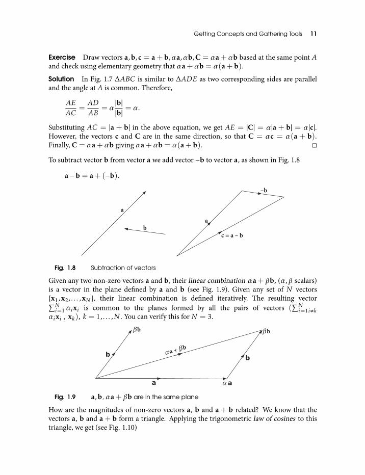
1.7 αa+αb = α(a+b) 101.8 Subtraction of vectors 111.9 a,b, αa+ βb are in the same plane 11
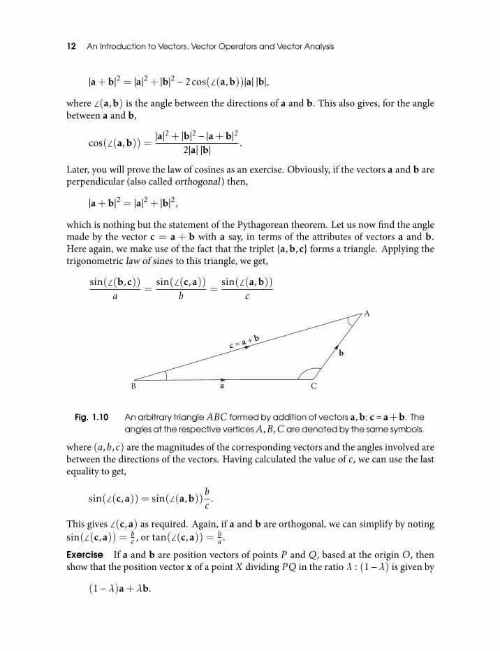
1.10 An arbitrary triangle ABC formed by addition of vectors a,b; c = a+b. Theangles at the respective vertices A,B,C are denoted by the same symbols. 12
1.11 Dividing PQ in the ratio λ : (1−λ) 131.12 Addition of forces to get the resultant. 171.13 (a) The velocity of a shell fired from a moving tank relative to the ground.
(b) The southward angle θ at which the shell will fire from a moving tank sothat its resulting velocity is due west. 17
1.14 (a) Left handed screw motion and (b) Left handed coordinate system.(c) Right handed screw motion and (d) Right handed (dextral) coordinate
xiv Figures
system. Try to construct other examples of the left and right handedcoordinate systems. 19
1.15 Scalar product is commutative. The projections of a on b and b on a giverespectively a·b = |a|cosθ and b·a = |b|cosθ. Multiplication on both sidesof the first equation by |b| and the second by |a| results in the symmetricalform a ·b = |b| a · b = |a| b · a 23
1.16 The scalar product is distributive with respect to addition 251.17 Lines joining a point on a sphere with two diametrically opposite points are
perpendicular 271.18 Getting coordinates of a vector v (see text) 271.19 Euclidean distance for vectors 281.20 Work done on an object as it is displaced by d under the action of force F 301.21 Potential energy of an electric dipole p in an electric field E 311.22 Torque on a current carrying coil in a magnetic field 311.23 Vector product of a and b : |a×b| = |a||b|sinθ is the area of the parallelogram
as shown 321.24 Generalizing the geometric interpretation of vector product 361.25 Geometrical interpretation of coordinates of a vector product 371.26 Moment of a force 381.27 Geometric interpretation of the scalar triple product (see text) 401.28 The volume of a tetrahedron as the scalar triple product 411.29 See text 501.30 Spherical polar coordinates 581.31 Coordinate surfaces are x2 + y2 + z2 = r2 (spheres r = constant) tanθ =
(x2+y2)1/2/z (circular cones, θ = constant) tanφ = y/x (half planesφ =constant) 60
1.32 Differential displacement corresponds to |ds|= |dr| (see text) 621.33 Parabolic coordinates (µ,ν,φ). Coordinate surfaces are paraboloids of
revolution (µ= constant,ν = constant) and half-planes (φ = constant) 631.34 Cylindrical coordinates (ρ,φ,z). Coordinate surfaces are circular cylinders
(ρ = constant), half-planes (φ = constant) intersecting on the z-axis, andparallel planes (z = constant) 64
1.35 Prolate spheroidal coordinates (η,θ,φ). Coordinate surfaces are prolatespheroids (η = constant), hyperboloids (θ = constant), and half-planes(φ = constant) 65
1.36 Oblate spheroidal coordinates (η,θ,φ). Coordinate surfaces are oblatespheroids (η = constant), hyperboloids (θ = constant), and half-planes(φ = constant) 66
Figures xv
1.37 (a) Positively and (b) negatively oriented triplets (a,b,c), (c) Triplet (b,a,c)has orientation opposite to that of (a,b,c) in (a) 68
2.1 LineL with directance d = x− (u · x)u 762.2 |m|= |x× u|= |d| for all x on the lineL 762.3 See text 772.4 See text 782.5 With A and B defined in Eq. (2.8) (a) |a×b|= |A|+ |B| and (b) |a×b|= |B|−|A|. These equations can be written in terms of the areas of the correspondingtriangles 80
2.6 A′ = (x− c)× (b− c) and B′ = (a− c)× (x− c) (see text) 812.7 Case of c parallel to x 822.8 See text 832.9 A plane positively oriented with respect to the frame (i, j, k) 83
2.10 Every line in the plane is normal to a 852.11 As seen from the figure, for every point on the plane k · r = constant 862.12 Shortest distance between two skew lines 882.13 A spherical triangle 892.14 Depicting Eq. (2.22) 912.15 Conics with a common focus and pericenter 92
3.1 Isomorphism between the complex plane Z and E2 953.2 Finding evolute of a unit circle 953.3 Finding
√i 96
3.4 Finding nth roots of unity 973.5 z,z∗, z ± z∗ 973.6 Depicting Eq. (3.3) 993.7 If D is real, z1,z2,z3,z4 lie on a circle 1003.8 The argument ∆ of ω defined by Eq. (3.9) 1023.9 Constant angle property of the circle 104
3.10 Constant power property of the circle 1043.11 Illustrating Eq. (3.10) 1053.12 Both impedance and admittance of this circuit are circles 1063.13 Boucherot’s circuit 1073.14 Four terminal network 1083.15 Geometrical meaning of ω2
z = ω0ω∞ 1093.16 Point by point implementation of transformation Eq. (3.14) 1103.17 An ellipse and a hyperbola 110
4.1 Inverse of a mapping. A one to one and onto map f : X 7→ Y has the uniqueinverse f −1 : Y 7→ X 118
xvi Figures
5.1 u ·(eiθv
)=
(e−iθu
)· v 141
5.2 Symmetric transformation with principal values λ1 > 1 and λ2 < 1 1455.3 An ellipsoid with semi-axes λ1,λ2,λ3 1465.4 Parameters in Mohr’s algorithm 1505.5 Mohr’s Circle 1515.6 Verification of Eq. (5.48) 1526.1 Reflection of a vector in a plane 1616.2 Reflection of a particle with momentum p by an unmovable plane 1626.3 See text 1646.4 Shear of a unit square 1696.5 Rotation of a vector 1706.6 Infinitesimal rotation δθ of x about n 1716.7 Vectors dx and arc length ds as radius |x|sinθ is rotated through angle δθ.
As δθ 7→ 0 dx becomes tangent to the circle. 1726.8 Orthonormal triad to study the action of the rotation operator 1746.9 Equivalent rotations: One counterclockwise and the other clockwise 178
6.10 Composition of rotations. Rotations do not commute. 1806.11 Active and passive transformations 1826.12 Euler angles 1846.13 Rotations corresponding to Euler angles 1866.14 Roll, pitch and yaw 187
7.1 (a) Symmetry elements of an equilateral triangle i) Reflections in three planesshown by ⊥ bisectors of sides. ii) Rotations through 2π/3,4π/3 and 2π(= identity) about the axis ⊥ to the plane of the triangle passing through thecenter. (b) Isomorphism with S3 (see text). 194
7.2 (a) Symmetry elements of a square (group D4) i) Reflections in planesthrough the diagonal and bisectors of the opposite sides. ii) Rotations aboutthe axis through the center and⊥ to the square by angles π/2,pi,3π/2 and2π (= identity). (b) D4 is isomorphic with a subgroup of S4 (see text). 195
7.3 Translation of a physical object by a 1997.4 A rigid displacement is the composite of a rotation and a translation. The
translation vector a need not be in the plane of rotation. 2017.5 Equivalence of a rotation/translation in a plane to a pure rotation 2038.1 A converging sequence in E3 2189.1 Geometry of the derivative 2229.2 Parameterization by arc length 2269.3 The Osculating circle 2289.4 Curvature of a planar curve 229
Figures xvii
9.5 A possible path of the satellite 2359.6 Projections of a space curve on the coordinate planes of a moving trihedral 2429.7 A construction for finding the equation of an involute C2 for a given evolute
C1 and vice versa 2449.8 Construction of a evolute-involute pair 2459.9 Finding the evolute of an involute 247
9.10 Ellipse 2499.11 Parameters relative to foci 2509.12 (a) Drawing ellipse with a pencil and a string (b) Semilatus rectum
(c) Polar coordinates relative to a focus 2519.13 Cycloid 2549.14 Epicycloid. Vectors are (i) : c, (ii) : a, (iii) : a+ c, (iv) : −R(t, n)c, (v) :
R(t, n)(a+ c), (vi) :R( ac t, n)(−R(t, n)c), (vii) : x(t) 2559.15 Cardioid 2569.16 Hypocycloid 2569.17 A point P on the rim of a circle rolling inside a circle of twice the radius
describes a straight line segment 2579.18 Trochoid 2589.19 A curve with a loop 2599.20 Positive sense of traversing a closed curve 2599.21 Positive and negative sides of an oriented arc 2609.22 Orientated simple closed curve 2609.23 Orientation of a curve with loops 2619.24 Positive direction of the tangent and the normal 2629.25 (a) A convex function with positive curvature, and (b) a concave function
with negative curvature 26210.1 Sections of u = f (x,y) 26710.2 Mapping polar to cartesian coordinates 27710.3 The gradient vector is orthogonal to the equipotential at every point 28210.4 Neighborhood of point (a,b) on f (x,y) = c is locally given by the implicit
function y = f (x) 28610.5 Stereographic projection of the sphere 29910.6 (a) Hyperboloid of one sheet and (b) Hyperboloid of two sheets 30010.7 Creation of torus by the rotation of a circle 30310.8 Vector fields given by (a) va (b) vb (c) vc as defined in this exercise 30510.9 Illustrating curl of a vector field 307
10.10 Various cases of field curling around a point 307
xviii Figures
10.11 The Network of coordinate lines and coordinate surfaces at any arbitarypoint, defining a curvilinear coordinate system 314
10.12 (a) Evaluating x · da (b) Flux through the opposite faces of a volume element 31810.13 Circulation around a loop 320
11.1 Defining the line integral 32311.2 x(t) = cos ti+ sin tj 32511.3 A circular helix 32611.4 In carrying a test charge from a to b the same work is done along either path 32611.5 Line integral over a unit circle 32811.6 Line integral around a simple closed curve as the sum of the line integrals
over its projections on the coordinate planes 33011.7 Illustrating Eq. (11.13) 33311.8 Each winding of the curve of integration around the z axis adds 2π to its
value 33511.9 Illustration of a simply connected domain 337
11.10 The closed loop for integration 34011.11 The geometry of Eq. (11.17) 34211.12 A spherically symmetric mass distribution 34711.13 Variables in the multipole expansion 35211.14 Earth’s rotation affected its shape in its formative stage 35411.15 Area integral 35811.16 Area swept out by radius vector along a closed curve. Cross-hatched region
is swept out twice in opposite directions, so its area is zero. 35911.17 Directed area of a self-intersecting closed plane curve. Vertical and
horizontal lines denote areas with opposite orientation, so cross-hatchedregion has zero area. 360
11.18 Interior and exterior approximations to the area of the unit disc |x| ≤ 1 forn= 0,1,2 where A−0 = 0,A−1 = 1,A−2 = 2,A+
2 = 4.25,A+1 = 6,A+
0 = 12 36111.19 Evaluation of a double integral 36411.20 Subdivision by polar coordinate net 36711.21 General convex region of integration 37411.22 Non-convex region of integration 37511.23 Circular ring as a region of integration 37511.24 Triangle as a region of integration 37611.25 The right triangular pyramid 37811.26 Changing variables of integration (see text) 37911.27 Tangent plane to the surface 38511.28 Divergence theorem for connected regions 396
Figures xix
11.29 n defines the directional derivatives of x and y 39711.30 Γ is the boundary of a simply connected region 40011.31 Amount of liquid crossing segment I in time dt for uniform flow of velocity v 40211.32 (a) Flow with sink and (b) flow with vortex 40511.33 Unit vector n gives the orientation of oriented surface S∗ at P 40811.34 Orientation of S with respect to u,v 41111.35 Mobius strip 41211.36 Illustrating Eq. (11.157) 41911.37 Evaluation of a line integral using Stoke’s theorem 439
12.1 The rotating fan 44712.2 Finding the instantaneous axis of rotation of a rigid body 44812.3 Orbit of an isotropic harmonic oscillator 45312.4 Elliptical orbit as a superposition of coplanar circular orbits 45312.5 (a) The regions V ≤ E, V1 ≤ E and V2 ≤ E (b) Construction of a Lissajous
figure 45512.6 Trajectory in position space 45712.7 Trajectory in the velocity space 45712.8 Graphical determination of the displacement r , time of light t and final
velocity v 45812.9 Terrestrial Coriolis effect 462
12.10 Topocentric directional parameters 46312.11 Net acceleration of river water 46812.12 Eliptical orbit and Hodograph 47212.13 Orbits after impulse 47312.14 Earth’s atmospheric drag on a satellite circularising its orbit 47412.15 Velocity vector precesses about ω 47612.16 (a) Right handed helix (b) Left handed helix 47712.17 Rotational velocity of a charge q about ω 47812.18 Trajectory of a charged particle in uniform electric and magnetic fields 48012.19 Directions of electric and magnetic fields for Fig. 12.18 48112.20 Trochoids traced by a charge q when the electric and magnetic fields are
orthogonal 48112.21 Two-dimensional flow around a 90 corner 48512.22 Two-dimensional flow around a 60 corner 48512.23 Two-dimensional flow around a Semi-infinite straight line 48612.24 Two-dimensional flow around a 2-D doublet source consisting of a source
and a sink of equal strength, at an infinitesimal separation 486
Tables
2.1 Classification of Conics and Conicoids 9212.1 Classification of Orbits with H , 0 471
Preface
This is a textbook on vectors at the undergraduate/advanced undergraduate level. Itstarget readership is the undergraduate student of science and engineering. It may also beused by professional scientists and engineers to brush up on various aspects of vectors andapplications of their interest. Vectors, vector operators and vector analysis form theessential background to and the skeleton of many courses in science and engineering.Therefore, the utility of a book which clearly builds up the theoretical structure andapplications of vectors cannot be over-emphasized. The present book is an attempt tofulfill such a requirement. This book, for instance, can be used to give a course forming acommon pre-requisite for a number of science and engineering courses. In this book, Ihave tried to develop the theory and applications of vectors from scratch. Although thesubject is presented in a general setting, it is developed in 3-D space using basic vectoralgebra. A coordinate-free approach is taken throughout, so that all developments are freeof any particular coordinate system and apply to all coordinate systems. This approachdirectly deals with vectors instead of their components or coordinates and combines thesevectors using vector algebra.
A large part of this book is inspired by the geometric algebra of multivectors thatoriginated in the 19th century, in the works of Grassmann and Clifford and which has hada powerful re-incarnation with enhanced applicability in the recent works of D. Hestenesand others [7, 10, 11]. This is one of the most general algebraic formulations of geometryof which vectors form a special case. Keeping the multivector geometric algebra at thebackdrop makes the coordinate free approach for vectors emerge naturally. On a personalnote, the book on classical mechanics by D. Hestenes [10], which introduced me to themultivector geometric algebra, has always been a source of joy and education for me.I have always enjoyed solving problems from this book, many of them are included here.In fact I have used Hestenes’ work in various places throughout the book, without using orreferring to the geometric algebra or geometric calculus.
While designing this book I was guided by two principles: A consistent development ofthe subject from scratch, and also showing the beauty of the whole edifice and extendingthe utility of the book to the largest possible cross-section of students. The book comprisesthree parts, one for each part of the title: First on the basic formulation, the second on
xxii Preface
vector operators and the third on vector analysis. Following is the brief description of eachone of them.
The first part gives the basic formulation, both conceptual and theoretical. The firstchapter builds basic concepts and tools. The first three sections are the result of myexperience with students and I have found that these matters should be explicitly dealtwith for the correct understanding of the subject. I hope that the first three sections willclear up the confusion and the misconceptions regarding many basic issues, in the mindsof students. I have also given the applications and examples of every algebraic operation,starting from vector addition. Levi-Civita notation is introduced in detail and used to getthe vector identities. The metric space structure is introduced and used to understandvectors in the context of the physical quantities they represent. Apart from the essentialstructures like basis, dimension, coordinate systems and the consequences of linearity, thecurvilinear coordinate systems like spherical polar and parabolic systems are developedsystematically. Vector fields are defined and their basic structure is given. The orientationof a linearly independent triplet of vectors is then discussed, also including the orientationof a triplet relative to a coordinate system and the related concept of the orientation of aplane, which is later used to understand the orientation of a surface. The second chapterdeals with the analytical geometry of curves and surfaces emphasizing vector methods.The third chapter uses complex algebra for manipulating planar vectors and for thedescription and transformations of the plane curves. In this chapter I follow the treatmentby Zwikker [26] which is a complete and rigorous exposition of these issues.
The second part deals with operators on vectors. Everything about vector operators isformulated using vector algebra (scalar and vector products) and matrices. The fourthchapter gives the algebra of operators and various types of operators, and proves andemphasizes the equivalence between the algebra of vector operators and the algebra ofmatrices representing them. The fifth chapter gives general formulation of gettingeigenvectors and eigenvalues of a linear operator on vectors using vector algebra. Theproperties of the spectrum of a symmetric operator are also obtained using vector algebra.Thus, extremely useful and general methods are accessible to the students usingelementary vector algebra. A powerful algorithm to diagonalize a positive operator actingon a 2-D space, called Mohr’s algorithm, is then described. Mohr’s algorithm has beenroutinely used by engineers via its graphical implementation, as explained in the text. Thesixth chapter develops in detail orthogonal transformations as rotations or reflections. Thegeneric forms for operators of reflection and rotation, as well as the matrices for therotation operator are obtained. The relationship between rotation and reflection isestablished via Hamilton’s theorem. The active and passive transformations and theirconnection with symmetry is discussed. The concept of broken symmetry is brieflydiscussed. The Euler angle construction for arbitrary rotation is then derived. Theproblem of finding the axis and the angle of rotation corresponding to a given orthogonalmatrix is solved as the Euler’s theorem. The second part ends with the seventh chapter ontransformation groups and deals with the rotation group, group of isometries and theEuclidean group, with applications to rigid displacements.
Preface xxiii
The third part deals with vector analysis. This is a vast subject and a personal flavor inthe choice of topics is inevitable. For me the guiding question was, what vector analysis agraduating student in science and engineering must have ? Again, the variety of answers tothis question is limited only by the number of people addressing it. Thus, the third partgives my version of the answer to this question and the resulting vector analysis. Iprimarily develop the subject with geometric point of view, making as much contact withapplications as possible. My aim is to enable the student to independently read,understand and use the literature based on vector analysis for the applications of hisinterest. Whether this aim is met can only be decided by the students who learn and try touse this material. This part is divided into five (Chapters 8–12). The eighth chapteroutlines fundamental notions and preliminary start ups, and also sets the objectives. Theninth chapter consists of the vector valued functions of a scalar variable. Theories of spacecurves and of plane curves are developed from scratch with some physical applications.This chapter ends with the integration of such functions with respect to their scalarargument and their Taylor series expansion. The tenth chapter deals with the functions ofvector argument, both scalar valued and vector valued, thus covering both the scalar andvector fields. Again, everything is developed from scratch, starting with the directionalderivative, partial derivatives and continuity of such functions. A part of this developmentis inspired by the geometric calculus developed by D. Hestenes and others [7, 10, 11]. Tosummarize, this chapter consists of different forms of derivatives of these and inversefunctions, and their geometric/physical applications. A major omission in this chapter isthat of the systematic development of differential forms, which may not be required in anundergraduate course. The eleventh chapter concerns vector integration. This is done inthree phases: the line, the surface and the volume integral. All the standard topics arecovered, emphasizing geometric aspects and physical applications. While writing this part,I have made use of many books, especially the book by Courant and John [5] and that byLang [15], for the simple reason that I have learnt my calculus from these books, and Ihave no regrets about that. In particular, my treatment of multiple integrals and matricesand determinants in Appendix A is inspired by Courant and John’s book. I find in theirbook, the unique property of building rigorous mathematics, starting from an intuitivegeometric picture. Also, I follow Griffiths while presenting the divergence and the curl ofvector fields, which, I think, is possibly one of the most compact and clear treatments ofthis topic. The subsections 11.1.1 and 11.8.1 and a part of section 9.2 are based on ref[22]. The twelfth and last chapter of the book presents an assorted collection ofapplications involving rotational motion of a rigid body, projectile motion, satellites andtheir orbits etc, illustrating coordinate-free analysis using vector techniques. This chapter,again, is influenced by Hestenes [10].
Appendix A develops the theory of matrices and determinants emphasizing theirconnection with vectors, also proving all results involving matrices and determinants usedin the text. Appendix B gives a brief introduction to Dirac delta function.
The whole book is interspersed with exercises, which form an integral part of the text.Most of these exercises are illustrative or they explore some real life application of thetheory. Some of them point out the subtlties involved. I recommend all students to attempt
xxiv Preface
all exercises, without looking at the solutions beforehand. When you read a solution afteran attempt to get there, you understand it better. Also, do not be miserly about drawingfigures, a figure can show you a way which thousand words may not.
I cannot end this preface without expressing my affection towards my friend and mydeceased colleague Dr Narayan Rana, who re-kindled my interest in mechanics. Longevenings that I spent with him discussing mechanics and physics in general, sharing andlaughing at various aspects of life from a distance, are the treasures of my life. We entereda rewarding and fruitful collaboration of writing a book on mechanics [19]. Thiscollaboration and Hestenes’ book [10] motivated me to formulate mechanics in acoordinate free way using vector methods. Apart from the book by Hestenes and his otherrelated work, the book by V. I. Arnold on mechanics [3] has made an indelible impact onmy understanding and my global view of mechanics, although its influence is not quiteapparent in this book. I have always enjoyed discussing mechanics and physics in generalwith my colleagues Rajeev Pathak, Anil Gangal, C. V. Dharmadhikari, P. Durganandini,and Ahmad Sayeed. The present book is produced in LATEX and I thank our students,Dinesh Mali, Mukesh Khanore and Mihir Durve for their help in drawing figures and alsoas TEXperts.
Nomenclature
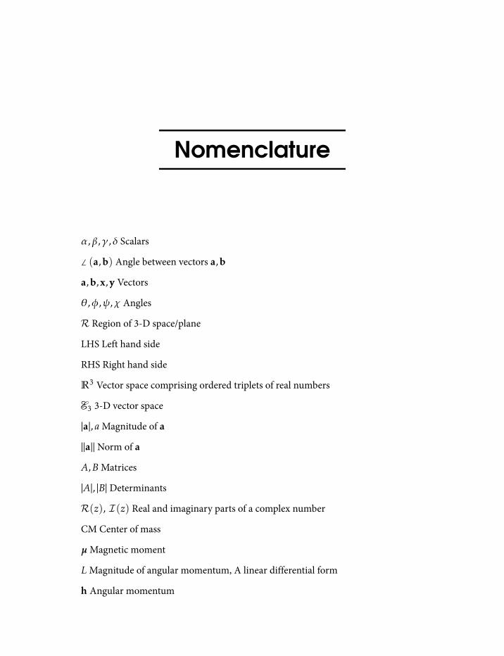
α,β,γ ,δ Scalars
∠ (a,b) Angle between vectors a,b
a,b,x,y Vectors
θ,φ,ψ,χ Angles
R Region of 3-D space/plane
LHS Left hand side
RHS Right hand side
R3 Vector space comprising ordered triplets of real numbers
E3 3-D vector space
|a|,aMagnitude of a
||a|| Norm of a
A,BMatrices
|A|, |B| Determinants
R(z), I (z) Real and imaginary parts of a complex number
CM Center of mass
µMagnetic moment
LMagnitude of angular momentum, A linear differential form
h Angular momentum
xxvi Nomenclature
H Specific angular momentum : Angular momentum per unit mass
M Moment of a force, Torque
B Magnetic field
E, E Electric field
κ Curvature
ρ Radius of curvature
p Semilatusrectum of a conic section
e Eccentricity of a conic section
m Moment of a line
R(n,θ) Operator for rotation of vector x about n by angle θ
U Canonical reflection operator, general orthogonal operator
S Similarity transformation on E3
A Affine transformation, skewsymmetric transformation
J Jacobian matrix
|J |, D Jacobian determinant
E, F, G Gaussian fundamental quantities of a surface
I Moment of Inertia operator/tensor
g(x, t) Gravitational field of a continuous body
Q Gravitational quadrupole tensor
ω, Ω Rotational velocity
Part I
Basic Formulation
Models are to be used, not believed.H. Theil (Principles of Econometrics)

1
Getting Concepts andGathering Tools
1.1 Vectors and ScalarsIn science and engineering we come across many quantities which require bothmagnitude and direction for their complete specification, e.g., velocity, acceleration,momentum, force, angular momentum, torque, electrical current density, electric andmagnetic fields, pressure and temperature gradients, heat flow and so on. To deal withsuch quantities, we need laws to represent, combine and manipulate them. Instead ofcreating these laws separately for each of these quantities, it makes good sense to create amathematical model to set up common laws for all quantities requiring both magnitudeand direction to be specified. This idea is neither new nor alien: right from our childhoodwe deal with real numbers and integers which are the mathematical objects representing avalue of ‘something’. This ‘something’ is anything which can be quantified or measuredand whose value is specified as a single entity: length, mass, time, energy, area, volume,curvature, cash in your pocket, the size of the memory and the speed of your computer,bank interest rates · · · . The combination and manipulation of these values is effected bycombining and manipulating the corresponding real numbers. Similarly, the values of thequantities specified by magnitude and direction are represented by vectors. A vector iscompletely specified by its magnitude and direction. Note that the magnitude of a vector isspecified by a single real number ≥ 0, so if we wish to change only the magnitude of avector, we must have the facility to multiply a vector by a real number, which we call ascalar in this context. Henceforth, in this book, by a scalar we mean a real number. Thus,in order to develop an algebra on the set of vectors, we need to associate with it the set ofscalars and define the laws for multiplying a vector by a scalar. If we multiply a vector by−1 we get the vector with same magnitude but opposite in direction, which, when addedto the original vector gives the zero vector, that is, a vector with zero magnitude and nodirection. Two vectors are equal if they have equal magnitudes and the same direction.
4 An Introduction to Vectors, Vector Operators and Vector Analysis
In this book we are using boldfaced letters for vectors. A symbol which is not bold, mayrepresent the magnitude of the corresponding vector, or a scalar.
1.2 Space and DirectionWe have not attempted to formally define ‘space’ or ‘direction’ as these are the integralparts of our experience right from birth. By space we mean the space we live in and movearound. We experience direction by our motion as well as by observing other movingobjects. We call our space three dimensional, (3-D) because given any two differentdirections, we can always choose a third direction such that going through any sequenceof displacements along any two of them, we will never move along the third and alsobecause given any set of four different directions we can always find a sequence ofdisplacements through any three of them, which will take us along the fourth. In thisbook, any n-dimensional object is denoted n-D. We also assume that space is acontinuum, that is, any region of space can be divided arbitrarily and indefinitely intosmaller and smaller regions. Further, we assume that space is an inert vacuum, whose solepurpose is to make room for different physical phenomena to occur in it. We denote thisspace by a symbol R3. You may wonder about this weird symbol. However, we willunderstand it in due course. For the time being we just view this symbol as a short namefor our space with the above properties.
In order to incorporate the concept of direction in our model, we note that any straightline in space specifies two directions, each by the sense in which the line is traversed. Inorder to pick one of these two directions, we may put an arrow-head on the line, pointingin the direction we want to indicate. Thus, a straight line with an arrow is our first modelfor specifying direction in space (see Fig. 1.1(a)). We will refine it shortly. Note that if weparallelly transport a line with an arrow, (that is, the transported line is always parallel tothe original one), it indicates the same direction. Thus, two different directions in spacecorrespond to two intersecting straight lines with arrows appropriately placed on them.One of these directions (which we call ‘reference direction’) can be reached from the otherby rotating the other direction about the line normal to the plane containing the twointersecting lines and passing through the point of intersection, until both, the lines andthe arrows, coincide (see Fig. 1.1(b)). The angular advance made by the rotating line issimply the angle between the two directions. This angle can be measured by drawing acircle of radius r in the plane of two intersecting lines with its center at the point ofintersection and measuring the length of the arc of this circle, say S, swept by the rotatingline. The angle θ swept by the rotating line is then given by
S = rθ.
Any arbitrary circle drawn in the specified plane can be used to get the value of angle θ viathe above equation (θ = S/r). In other words, the radius r is arbitrary. It is convenientto choose a unit circle, that is, a circle with radius unity, (r = 1), so that the arc-lengthand the angle swept by the rotating line are numerically equal (see Fig. 1.1(c)). Such a arc-length measure of angle is called ‘radian measure’. Since the length of the circumference
Getting Concepts and Gathering Tools 5
of a unit circle is 2π, the angle corresponding to one complete rotation is 2π. The anglecorresponding to half the circumference is π and so on.
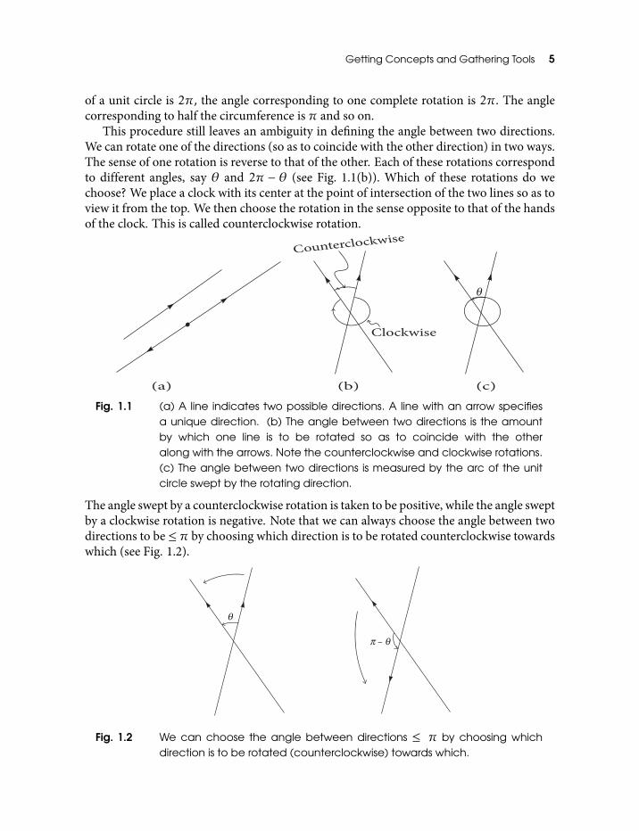
This procedure still leaves an ambiguity in defining the angle between two directions.We can rotate one of the directions (so as to coincide with the other direction) in two ways.The sense of one rotation is reverse to that of the other. Each of these rotations correspondto different angles, say θ and 2π − θ (see Fig. 1.1(b)). Which of these rotations do wechoose? We place a clock with its center at the point of intersection of the two lines so as toview it from the top. We then choose the rotation in the sense opposite to that of the handsof the clock. This is called counterclockwise rotation.
Fig. 1.1 (a) A line indicates two possible directions. A line with an arrow specifiesa unique direction. (b) The angle between two directions is the amountby which one line is to be rotated so as to coincide with the otheralong with the arrows. Note the counterclockwise and clockwise rotations.(c) The angle between two directions is measured by the arc of the unitcircle swept by the rotating direction.
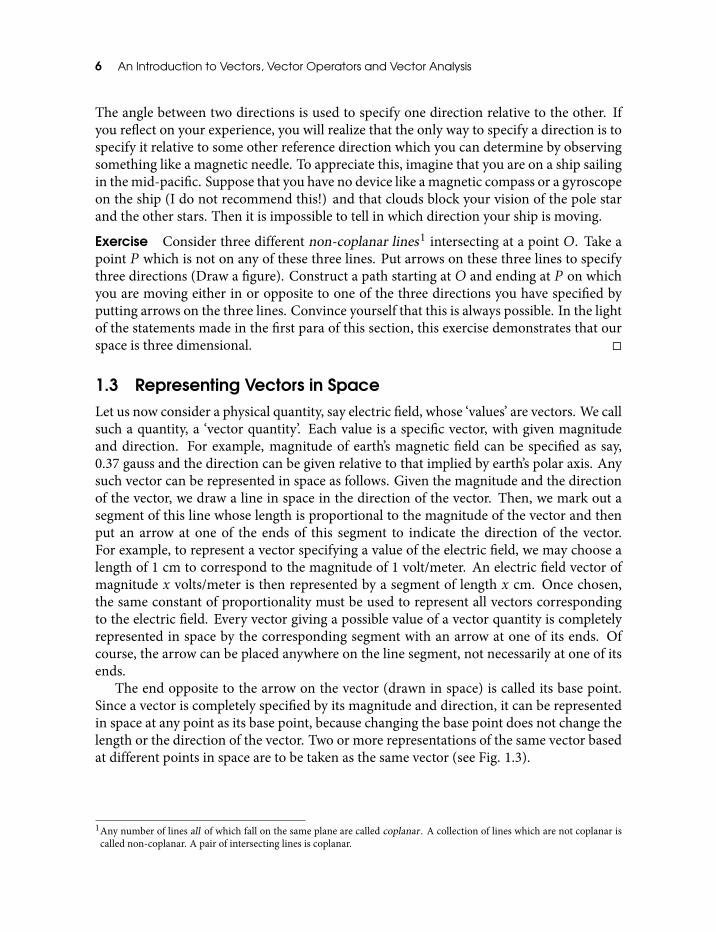
The angle swept by a counterclockwise rotation is taken to be positive, while the angle sweptby a clockwise rotation is negative. Note that we can always choose the angle between twodirections to be ≤ π by choosing which direction is to be rotated counterclockwise towardswhich (see Fig. 1.2).
Fig. 1.2 We can choose the angle between directions ≤ π by choosing whichdirection is to be rotated (counterclockwise) towards which.
6 An Introduction to Vectors, Vector Operators and Vector Analysis
The angle between two directions is used to specify one direction relative to the other. Ifyou reflect on your experience, you will realize that the only way to specify a direction is tospecify it relative to some other reference direction which you can determine by observingsomething like a magnetic needle. To appreciate this, imagine that you are on a ship sailingin the mid-pacific. Suppose that you have no device like a magnetic compass or a gyroscopeon the ship (I do not recommend this!) and that clouds block your vision of the pole starand the other stars. Then it is impossible to tell in which direction your ship is moving.
Exercise Consider three different non-coplanar lines1 intersecting at a point O. Take apoint P which is not on any of these three lines. Put arrows on these three lines to specifythree directions (Draw a figure). Construct a path starting at O and ending at P on whichyou are moving either in or opposite to one of the three directions you have specified byputting arrows on the three lines. Convince yourself that this is always possible. In the lightof the statements made in the first para of this section, this exercise demonstrates that ourspace is three dimensional.
1.3 Representing Vectors in SpaceLet us now consider a physical quantity, say electric field, whose ‘values’ are vectors. We callsuch a quantity, a ‘vector quantity’. Each value is a specific vector, with given magnitudeand direction. For example, magnitude of earth’s magnetic field can be specified as say,0.37 gauss and the direction can be given relative to that implied by earth’s polar axis. Anysuch vector can be represented in space as follows. Given the magnitude and the directionof the vector, we draw a line in space in the direction of the vector. Then, we mark out asegment of this line whose length is proportional to the magnitude of the vector and thenput an arrow at one of the ends of this segment to indicate the direction of the vector.For example, to represent a vector specifying a value of the electric field, we may choose alength of 1 cm to correspond to the magnitude of 1 volt/meter. An electric field vector ofmagnitude x volts/meter is then represented by a segment of length x cm. Once chosen,the same constant of proportionality must be used to represent all vectors correspondingto the electric field. Every vector giving a possible value of a vector quantity is completelyrepresented in space by the corresponding segment with an arrow at one of its ends. Ofcourse, the arrow can be placed anywhere on the line segment, not necessarily at one of itsends.
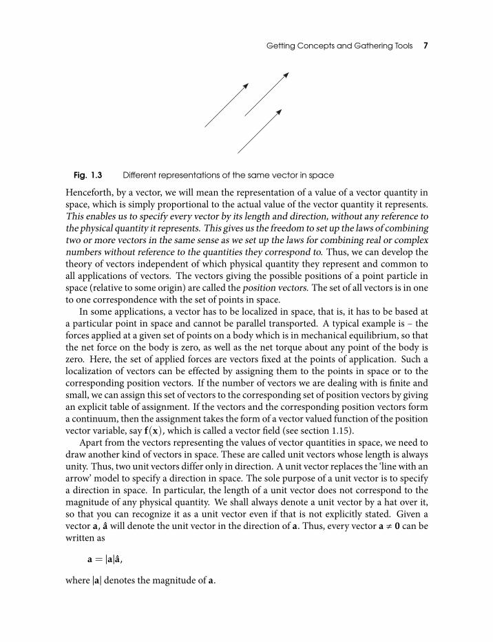
The end opposite to the arrow on the vector (drawn in space) is called its base point.Since a vector is completely specified by its magnitude and direction, it can be representedin space at any point as its base point, because changing the base point does not change thelength or the direction of the vector. Two or more representations of the same vector basedat different points in space are to be taken as the same vector (see Fig. 1.3).
1Any number of lines all of which fall on the same plane are called coplanar . A collection of lines which are not coplanar iscalled non-coplanar. A pair of intersecting lines is coplanar.
Getting Concepts and Gathering Tools 7
Fig. 1.3 Different representations of the same vector in space
Henceforth, by a vector, we will mean the representation of a value of a vector quantity inspace, which is simply proportional to the actual value of the vector quantity it represents.This enables us to specify every vector by its length and direction, without any reference tothe physical quantity it represents. This gives us the freedom to set up the laws of combiningtwo or more vectors in the same sense as we set up the laws for combining real or complexnumbers without reference to the quantities they correspond to. Thus, we can develop thetheory of vectors independent of which physical quantity they represent and common toall applications of vectors. The vectors giving the possible positions of a point particle inspace (relative to some origin) are called the position vectors. The set of all vectors is in oneto one correspondence with the set of points in space.
In some applications, a vector has to be localized in space, that is, it has to be based ata particular point in space and cannot be parallel transported. A typical example is – theforces applied at a given set of points on a body which is in mechanical equilibrium, so thatthe net force on the body is zero, as well as the net torque about any point of the body iszero. Here, the set of applied forces are vectors fixed at the points of application. Such alocalization of vectors can be effected by assigning them to the points in space or to thecorresponding position vectors. If the number of vectors we are dealing with is finite andsmall, we can assign this set of vectors to the corresponding set of position vectors by givingan explicit table of assignment. If the vectors and the corresponding position vectors forma continuum, then the assignment takes the form of a vector valued function of the positionvector variable, say f(x), which is called a vector field (see section 1.15).
Apart from the vectors representing the values of vector quantities in space, we need todraw another kind of vectors in space. These are called unit vectors whose length is alwaysunity. Thus, two unit vectors differ only in direction. A unit vector replaces the ‘line with anarrow’ model to specify a direction in space. The sole purpose of a unit vector is to specifya direction in space. In particular, the length of a unit vector does not correspond to themagnitude of any physical quantity. We shall always denote a unit vector by a hat over it,so that you can recognize it as a unit vector even if that is not explicitly stated. Given avector a, a will denote the unit vector in the direction of a. Thus, every vector a , 0 can bewritten as
a = |a|a,
where |a| denotes the magnitude of a.
8 An Introduction to Vectors, Vector Operators and Vector Analysis
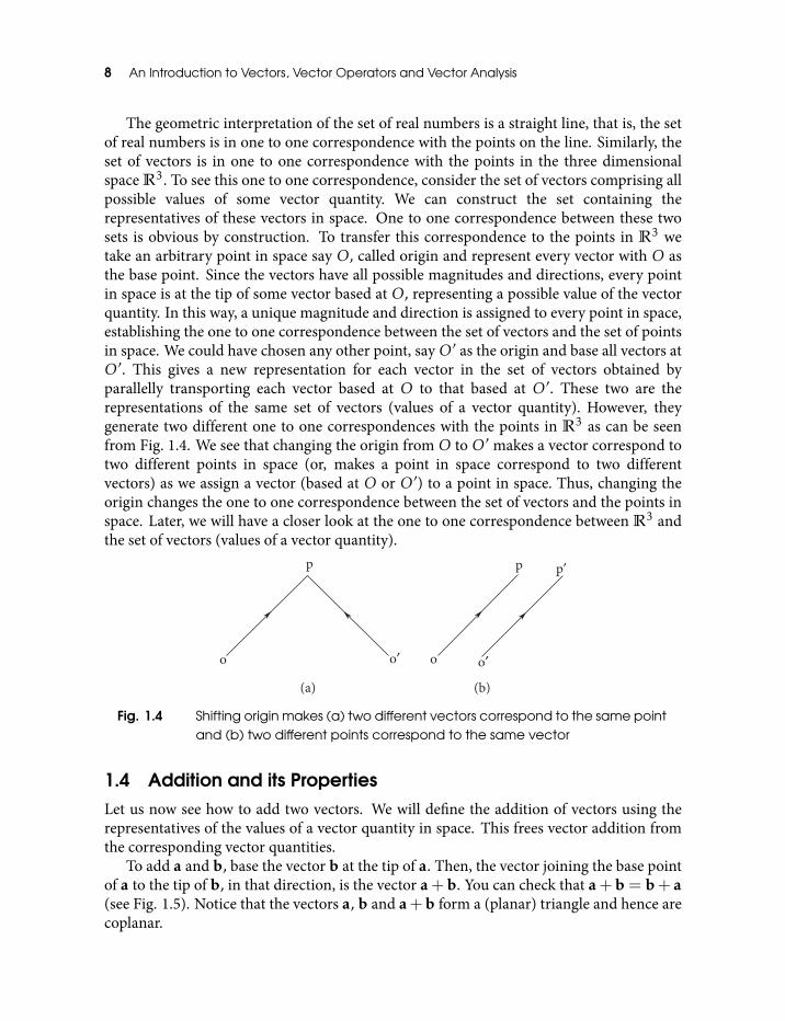
The geometric interpretation of the set of real numbers is a straight line, that is, the setof real numbers is in one to one correspondence with the points on the line. Similarly, theset of vectors is in one to one correspondence with the points in the three dimensionalspace R3. To see this one to one correspondence, consider the set of vectors comprising allpossible values of some vector quantity. We can construct the set containing therepresentatives of these vectors in space. One to one correspondence between these twosets is obvious by construction. To transfer this correspondence to the points in R3 wetake an arbitrary point in space say O, called origin and represent every vector with O asthe base point. Since the vectors have all possible magnitudes and directions, every pointin space is at the tip of some vector based at O, representing a possible value of the vectorquantity. In this way, a unique magnitude and direction is assigned to every point in space,establishing the one to one correspondence between the set of vectors and the set of pointsin space. We could have chosen any other point, sayO′ as the origin and base all vectors atO′. This gives a new representation for each vector in the set of vectors obtained byparallelly transporting each vector based at O to that based at O′. These two are therepresentations of the same set of vectors (values of a vector quantity). However, theygenerate two different one to one correspondences with the points in R3 as can be seenfrom Fig. 1.4. We see that changing the origin from O to O′ makes a vector correspond totwo different points in space (or, makes a point in space correspond to two differentvectors) as we assign a vector (based at O or O′) to a point in space. Thus, changing theorigin changes the one to one correspondence between the set of vectors and the points inspace. Later, we will have a closer look at the one to one correspondence between R3 andthe set of vectors (values of a vector quantity).
Fig. 1.4 Shifting origin makes (a) two different vectors correspond to the same pointand (b) two different points correspond to the same vector
1.4 Addition and its PropertiesLet us now see how to add two vectors. We will define the addition of vectors using therepresentatives of the values of a vector quantity in space. This frees vector addition fromthe corresponding vector quantities.
To add a and b, base the vector b at the tip of a. Then, the vector joining the base pointof a to the tip of b, in that direction, is the vector a+b. You can check that a+b = b+ a(see Fig. 1.5). Notice that the vectors a, b and a+b form a (planar) triangle and hence arecoplanar.
Getting Concepts and Gathering Tools 9
Fig. 1.5 Vector addition is commutative
The vector a + b is sometimes called the resultant of a and b. The rule of adding two ormore vectors is motivated by the net displacement of an object in space, resulting due tomany successive displacements. Thus, if we go from A to B by travelling 10km NE (vectora) and then from B to C by travelling 6km W (vector b) the net displacement, 8km dueNorth from A to C (vector c), is obtained as depicted in Fig. 1.6(a), which is the same asthat given by c = a+ b. Figure 1.6(b) shows the net displacement (f) after four successivedisplacements (a,b,c,d) which is consistent with f = a+b+ c+d.
We can now list the properties of vector addition and multiplication by a scalar.
(1) Closure If a,b are in R3 then a + b is also in R3. That is, addition of two vectorsresults in a vector.
(2) Commutativity a+b = b+ a (see Fig. 1.5).(3) Associativity For all vectors a,b,c in R3, a + (b + c) = (a + b) + c. Thus, while
adding three or more vectors, it does not matter which two you add first, which twonext etc, that is, the order in which you add does not matter (see Fig. 1.6(b)).
(4) Identity There is a unique vector 0 such that for every vector a in R3, a+ 0 = a.
(5) Inverse For every vector a , 0 in R3, there is a unique vector −a such that a +(−a) = 0 and 0± 0 = 0.
To every pair α and a where α is a scalar (i.e., a real number) and a in R3 there is a vectorαa in R3. If we denote by |a| the magnitude of a, then the magnitude of αa is |α| |a|. Ifα > 0, the direction of αa is the same as that of a, while if α < 0 then the direction of αais opposite to that of a. If α > 0, then αa is said to be the scaling of a by α. Note that α =1/|a| produces unit vector a in the direction of a. We have, for the scalar multiplication,
(1) Associativity α(βa) = (αβ)a.
(2) Identity 1a = a.
10 An Introduction to Vectors, Vector Operators and Vector Analysis
Fig. 1.6 (a) Addition of two vectors (see text). (b) Vector AE equals a+b+ c+d.Draw different figures, adding a,b,c,d in different orders to check that thisvector addition is associative.
Multiplication by scalars is distributive, namely,
(3) α(a+b) = αa+αb.
(4) (α+ β)a = αa+ βa.
Fig. 1.7 αa+αb = α(a+b)
Note that these properties are shared by all vectors independent of the context in whichthey are used and independent of which vector quantity they correspond to. As explainedin section 1.3, this is true of all the algebra of vectors and operations on vectors we developin this book and will not be stated explicitly again.
Getting Concepts and Gathering Tools 11
Exercise Draw vectors a,b,c = a+ b,αa,αb,C = αa+αb based at the same point Aand check using elementary geometry that αa+αb = α(a+b).
Solution In Fig. 1.7 ∆ABC is similar to ∆ADE as two corresponding sides are paralleland the angle at A is common. Therefore,
AEAC
=ADAB
= α|b||b|
= α.
Substituting AC = |a + b| in the above equation, we get AE = |C| = α|a + b| = α|c|.However, the vectors c and C are in the same direction, so that C = αc = α(a + b).Finally, C = αa+αb giving αa+αb = α(a+b).
To subtract vector b from vector a we add vector −b to vector a, as shown in Fig. 1.8
a−b = a+ (−b).
Fig. 1.8 Subtraction of vectors
Given any two non-zero vectors a and b, their linear combination αa+ βb, (α,β scalars)is a vector in the plane defined by a and b (see Fig. 1.9). Given any set of N vectorsx1,x2, . . . ,xN , their linear combination is defined iteratively. The resulting vector∑Ni=1αixi is common to the planes formed by all the pairs of vectors (
∑Ni=1i,k
αixi , xk), k = 1, . . . ,N . You can verify this forN = 3.
Fig. 1.9 a,b, αa+ βb are in the same plane
How are the magnitudes of non-zero vectors a, b and a + b related? We know that thevectors a, b and a + b form a triangle. Applying the trigonometric law of cosines to thistriangle, we get (see Fig. 1.10)
12 An Introduction to Vectors, Vector Operators and Vector Analysis
|a+b|2 = |a|2 + |b|2 − 2cos(∠(a,b))|a| |b|,
where ∠(a,b) is the angle between the directions of a and b. This also gives, for the anglebetween a and b,
cos(∠(a,b)) =|a|2 + |b|2 − |a+b|2
2|a| |b|.
Later, you will prove the law of cosines as an exercise. Obviously, if the vectors a and b areperpendicular (also called orthogonal ) then,
|a+b|2 = |a|2 + |b|2,
which is nothing but the statement of the Pythagorean theorem. Let us now find the anglemade by the vector c = a + b with a say, in terms of the attributes of vectors a and b.Here again, we make use of the fact that the triplet a,b,c forms a triangle. Applying thetrigonometric law of sines to this triangle, we get,
sin(∠(b,c))a
=sin(∠(c,a))
b=
sin(∠(a,b))c
Fig. 1.10 An arbitrary triangleABC formed by addition of vectors a,b; c = a+b. Theangles at the respective verticesA,B,C are denoted by the same symbols.
where (a,b,c) are the magnitudes of the corresponding vectors and the angles involved arebetween the directions of the vectors. Having calculated the value of c, we can use the lastequality to get,
sin(∠(c,a)) = sin(∠(a,b))bc
.
This gives ∠(c,a) as required. Again, if a and b are orthogonal, we can simplify by notingsin(∠(c,a)) = b
c , or tan(∠(c,a)) = ba .
Exercise If a and b are position vectors of points P and Q, based at the origin O, thenshow that the position vector x of a point X dividing PQ in the ratio λ : (1−λ) is given by
(1−λ)a+λb.
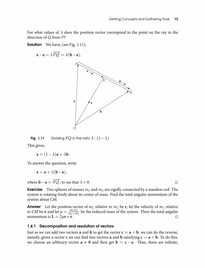
Getting Concepts and Gathering Tools 13
For what values of λ does the position vector correspond to the point on the ray in thedirection ofQ from P ?
Solution We have, (see Fig. 1.11),
x− a = λ−−→PQ = λ(b− a).
Fig. 1.11 Dividing PQ in the ratio λ : (1−λ)
This gives,
x = (1−λ)a+λb.
To answer the question, write
x = a+λ(b− a),
where b− a =−−→PQ , to see that λ > 0.
Exercise Two spheres of massesm1 andm2 are rigidly connected by a massless rod. Thesystem is rotating freely about its center of mass. Find the total angular momentum of thesystem about CM.
Answer Let the position vector of m1 relative to m2 be r, let the velocity of m1 relativeto CM be v and let µ = m1m2
m1+m2be the reduced mass of the system. Then the total angular
momentum is L = 2µr× v.
1.4.1 Decomposition and resolution of vectors
Just as we can add two vectors a and b to get the vector c = a + b, we can do the reverse,namely, given a vector c we can find two vectors a and b satisfying c = a + b. To do this,we choose an arbitrary vector a , 0 and then get b = c − a. Thus, there are infinite,
14 An Introduction to Vectors, Vector Operators and Vector Analysis
(in fact, uncountably many), pairs of vectors into which a given vector can be decomposedor resolved. In order to resolve a given vector c into a set of N vectors we first choosearbitrary sets αi , 0 and xi , 0, i = 1, . . . ,N − 1 of N − 1 scalars and vectorsrespectively and find the vector x =
∑N−1i=1 αixi . Then, we choose αN and xN to satisfy
αNxN = c − x. Thus, any vector can be resolved or decomposed in a set of N vectors ininfinitely (uncountably) many ways.
Exercise Draw figures illustrating c = αa+βb and d = αa+βb+γc for different setsof scalars and vectors satisfying these equations.
Exercise Given a vector c find two vectors a,b of given magnitudes a,b respectively, suchthat c is the resultant of a,b. When is this impossible?
Answer Squaring both sides of b = c − a we get, for the angle between a and c, c · a =
cosθ = (c2 + a2−b2)/2ca. Thus, if we draw vectors c =−−→AC and a =
−−→AB making angle
θ = cos−1[(c2+a2−b2)/2ca] with each other atA, then the vector−−→BC gives the required
vector b. This will fail if the vectors a,b,c cannot make a triangle, that is when a+b < c.
Exercise Given a vector a , 0 andN non-zero vectors xi , i = 1, . . . ,N , no two of whichare parallel and no three of which are coplanar, show that the linear combination of xi’sthat equals a is unique.
Solution We first show it for N = 2. Let a = λx1 + µx2. Note that both the coefficientscannot be zero, otherwise a = 0. Now suppose that some other linear combination equalsa, say a = λ1x1 + µ1x2. Subtracting these two equations we get (λ − λ1)x1+ (µ − µ1)x2 = 0. Either both of these coefficients are non-zero, or both are zero, otherwise one ofthe vectors x1,x2 is zero, contradicting the assumption that both are non-zero. If boththe coefficients are non-zero, then the vectors x1,x2 are simply proportional to each other,which means that they are parallel, in contradiction with the assumption that they are not.Therefore, both the coefficients (λ−λ1) and (µ−µ1) must vanish, proving that the linearcombination of x1 and x2 which equals a is unique. This also means that a given linearcombination specifies a unique vector a. Now let a equal a linear combination of threenon-zero and non-coplanar2 vectors, say a = λ1x1 +λ2x2 +λ3x3. We know that the firsttwo terms in this linear combination add up to a unique vector say x12 = λ1x1 + λ2x2.Therefore, we can equivalently write this linear combination as a = x12 + λ3x3 involvingonly two vectors which are not collinear because three vectors x1,x2,x3 are not coplanar,sothat we know it to be unique. This fixes the coefficient λ3 and hence makes the linearcombination of three vectors giving a unique. Iterating the same argument we can showthat a linear combination of non-zero, non-parallel and non-coplanar N vectors whichequals a is unique.
Exercise The center of mass of the vertices of a tetrahedron PQRS (each with unit mass)may be defined as the point dividing MS in the ratio 1 : 3, where M is the center of massof the vertices PQR. Show that this definition is independent of the order in which thevertices are taken and it agrees with the general definition of the center of mass.2Note that if three vectors are non-coplanar, then no two of them can be parallel.
Getting Concepts and Gathering Tools 15
Solution Let p,q,r,s,m be the position vectors of the points P ,Q,R,S,M respectively.Take the origin O at the point dividing MS in the ratio 1 : 3. Thus, s = −3m. Sincem = 1/3(p+q+ r), it follows that
14(p+q+ r+ s) = 0.
Thus, O is the center of mass by the general definition and clearly does not depend on theorder of the vertices.
Exercise Two edges of a tetrahedron are called opposite if they have no vertex incommon. For example, the edges PQ and RS of the tetrahedron of the previous exerciseare opposite. Show that the segment joining the midpoints of opposite edges of atetrahedron passes through the center of mass of the vertices.
Solution Let the edges be PQ and RS so that in the notation of the preceding solutiontheir midpoints have position vectors 1
2(p+q) and 12(r+s) respectively. From the solution
to the previous exercise 12(p + q) = −1
2(r + s); hence, the midpoints are collinear withcenter of massO and equidistant from it.
Exercise Let a1,a2, . . . ,an be the position vectors of n particles in space, with respect tothe origin at the center of mass G of this system, with masses m1,m2, . . . ,mn respectively.Show that
m1a1 +m2a2 + · · ·+mnan = 0.
Solution By definition, the left side gives the position vector of the center of mass G,which is chosen to be zero.
Collinear and coplanar vectors
Two non-zero vectors are collinear if they have same or opposite directions. Two suchvectors can be made to lie on the same line because a line accommodates two oppositedirections (orientations). Obviously, two collinear vectors a and b are proportional to eachother: b = ka with |b| = |k||a| and k > 0 (k < 0) corresponds to the two vectors in thesame (opposite) direction(s). We have to differentiate between collinear vectors we havejust defined and the collinear points in space which are points lying on the same line.
Three non-zero vectors are coplanar if they lie or can be made to lie in the same plane.Three vectors are non-coplanar if they are not coplanar. Let a,b,c be three non-zero vectorssuch that c can be resolved along a and b so that c is a linear combination
c = αa+ βb (1.1)
for some non-zero scalars α and β. This means, the vectors c, αa and βb form a triangle.Since triangle is a planar figure, we conclude that vectors a,b,c are coplanar. More usefulform of Eq. (1.1) is
αa+ βb+ γc = 0. (1.2)
16 An Introduction to Vectors, Vector Operators and Vector Analysis
On the other hand if a,b,c are given to be coplanar, it is possible to resolve one of themalong the other two vectors, as shown at the beginning of this subsection, so that theysatisfy Eq. (1.1) or Eq. (1.2) with α,β,γ not all zero. Thus, three non-zero vectors arecoplanar if and only if they satisfy Eq. (1.2) with two or more non-zero coefficients.It follows immediately that if three non-zero vectors satisfy Eq. (1.2) only when all thecoefficients are zero, then they aught to be non-coplanar.
Exercise Show that three points with position vectors a,b,c are collinear if and only ifthere exist three non-zero scalars α,β,γ , α , ±β, such that
αa+ βb+ γc = 0
andα+ β+ γ = 0.
Hint From a previous exercise we can infer that if three points are collinear, the positionvector of the middle point is b =
αc+γaα+γ giving γa + αc = (α+ γ)b or β + α+ γ = 0.
If the given conditions are assumed, we can show that b divides the line joining a and c inthe ratio α : γ .
Exercise Four points P ,Q,R,S have position vectors a,b,c,d respectively, no three ofwhich are collinear. Show that P ,Q,R,S are coplanar if and only if there exist four scalarsα,β,γ ,δ not all zero, satisfying
αa+ βb+ γc+ δd = 0 and α+ β+ γ + δ = 0. (1.3)
Solution Let the given P ,Q,R,S be coplanar and let the lines PQ and RS intersect atA with position vector r, such that PA : AQ = λ/µ and RA : AS = ρ/τ . By previousexercise this gives,
µa+λbλ+ µ
= r =τd+ ρcρ+ τ
,
orµ
λ+ µa+
λλ+ µ
b−ρ
ρ+ τc−
ρ
ρ+ τd = 0.
Replacing the coefficients by α,β,γ ,δ we see that conditions in Eq. (1.3) are satisfied. Theproof of sufficiency is left to you.
Vector methods employed to prove simple results in Euclidean geometry may be foundin [23].
1.4.2 Examples of vector addition
In this book we will draw examples from physics and engineering. This particularly suitsvectors as vectors are almost exclusively used in physics and engineering.
Getting Concepts and Gathering Tools 17
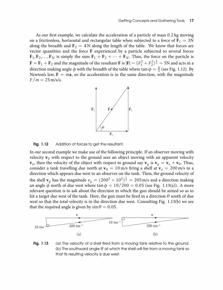
As our first example, we calculate the acceleration of a particle of mass 0.2 kg movingon a frictionless, horizontal and rectangular table when subjected to a force of F1 = 3Nalong the breadth and F2 = 4 N along the length of the table. We know that forces arevector quantities and the force F experienced by a particle subjected to several forcesF1,F2, . . . ,FN is simply the sum F1 + F2 + · · · + FN . Thus, the force on the particle isF = F1 + F2 and the magnitude of the resultant F is |F| = (F2
1 + F22)
12 = 5N and acts in a
direction making angle φ with the breadth of the table where tanφ = 43 (see Fig. 1.12). By
Newton’s law, F = ma, so the acceleration is in the same direction, with the magnitudeF/m= 25 m/s/s.
Fig. 1.12 Addition of forces to get the resultant.
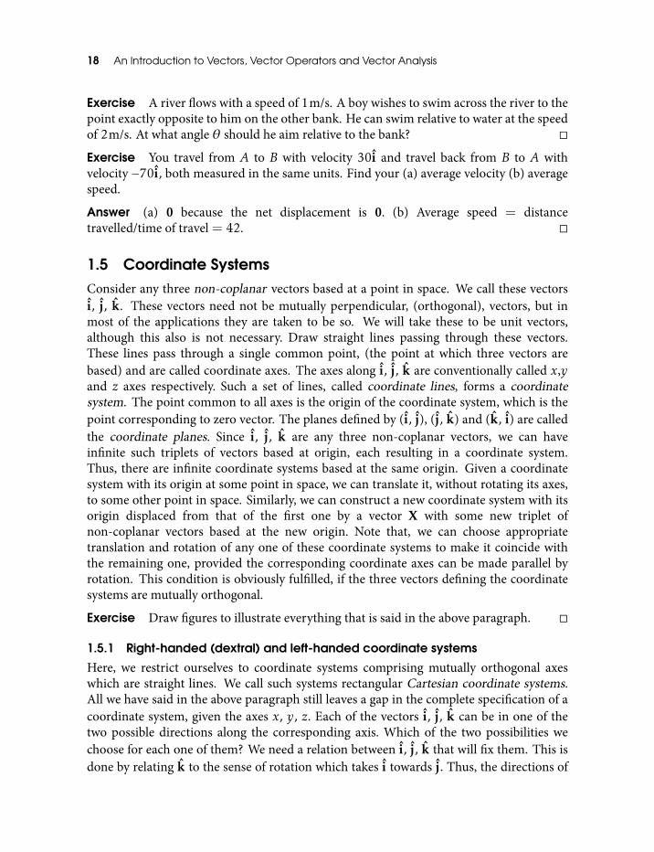
In our second example we make use of the following principle. If an observer moving withvelocity v0 with respect to the ground sees an object moving with an apparent velocityva, then the velocity of the object with respect to ground say vg is vg = va + v0. Thus,consider a tank travelling due north at v0 = 10 m/s firing a shell at va = 200 m/s in adirection which appears due west to an observer on the tank. Then, the ground velocity ofthe shell vg has the magnitude vg = (2002 + 102)
12 = 205 m/s and a direction making
an angle φ north of due west where tanφ = 10/200 = 0.05 (see Fig. 1.13(a)). A morerelevant question is to ask about the direction in which the gun should be aimed so as tohit a target due west of the tank. Here, the gun must be fired in a direction θ south of duewest so that the total velocity is in the direction due west. Consulting Fig. 1.13(b) we seethat the required angle is given by sinθ = 0.05.
Fig. 1.13 (a) The velocity of a shell fired from a moving tank relative to the ground.(b) The southward angle θ at which the shell will fire from a moving tank sothat its resulting velocity is due west.
18 An Introduction to Vectors, Vector Operators and Vector Analysis
Exercise A river flows with a speed of 1m/s. A boy wishes to swim across the river to thepoint exactly opposite to him on the other bank. He can swim relative to water at the speedof 2m/s. At what angle θ should he aim relative to the bank?
Exercise You travel from A to B with velocity 30i and travel back from B to A withvelocity −70i, both measured in the same units. Find your (a) average velocity (b) averagespeed.
Answer (a) 0 because the net displacement is 0. (b) Average speed = distancetravelled/time of travel = 42.
1.5 Coordinate SystemsConsider any three non-coplanar vectors based at a point in space. We call these vectorsi, j, k. These vectors need not be mutually perpendicular, (orthogonal), vectors, but inmost of the applications they are taken to be so. We will take these to be unit vectors,although this also is not necessary. Draw straight lines passing through these vectors.These lines pass through a single common point, (the point at which three vectors arebased) and are called coordinate axes. The axes along i, j, k are conventionally called x,yand z axes respectively. Such a set of lines, called coordinate lines, forms a coordinatesystem. The point common to all axes is the origin of the coordinate system, which is thepoint corresponding to zero vector. The planes defined by (i, j), (j, k) and (k, i) are calledthe coordinate planes. Since i, j, k are any three non-coplanar vectors, we can haveinfinite such triplets of vectors based at origin, each resulting in a coordinate system.Thus, there are infinite coordinate systems based at the same origin. Given a coordinatesystem with its origin at some point in space, we can translate it, without rotating its axes,to some other point in space. Similarly, we can construct a new coordinate system with itsorigin displaced from that of the first one by a vector X with some new triplet ofnon-coplanar vectors based at the new origin. Note that, we can choose appropriatetranslation and rotation of any one of these coordinate systems to make it coincide withthe remaining one, provided the corresponding coordinate axes can be made parallel byrotation. This condition is obviously fulfilled, if the three vectors defining the coordinatesystems are mutually orthogonal.
Exercise Draw figures to illustrate everything that is said in the above paragraph.
1.5.1 Right-handed (dextral) and left-handed coordinate systems
Here, we restrict ourselves to coordinate systems comprising mutually orthogonal axeswhich are straight lines. We call such systems rectangular Cartesian coordinate systems.All we have said in the above paragraph still leaves a gap in the complete specification of acoordinate system, given the axes x, y, z. Each of the vectors i, j, k can be in one of thetwo possible directions along the corresponding axis. Which of the two possibilities wechoose for each one of them? We need a relation between i, j, k that will fix them. This isdone by relating k to the sense of rotation which takes i towards j. Thus, the directions of
Getting Concepts and Gathering Tools 19
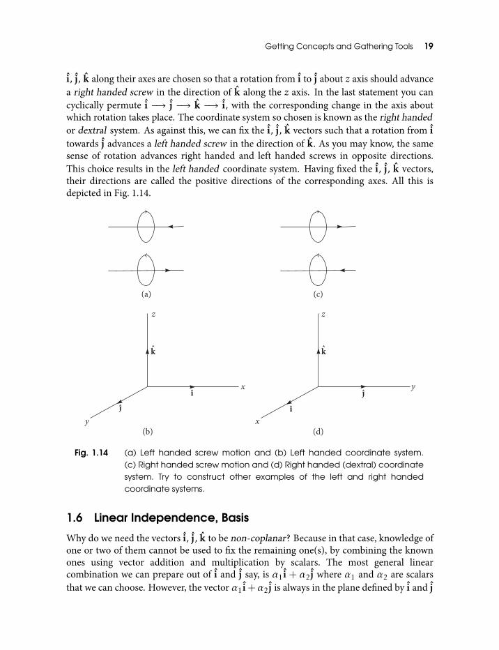
i, j, k along their axes are chosen so that a rotation from i to j about z axis should advancea right handed screw in the direction of k along the z axis. In the last statement you cancyclically permute i −→ j −→ k −→ i, with the corresponding change in the axis aboutwhich rotation takes place. The coordinate system so chosen is known as the right handedor dextral system. As against this, we can fix the i, j, k vectors such that a rotation from itowards j advances a left handed screw in the direction of k. As you may know, the samesense of rotation advances right handed and left handed screws in opposite directions.This choice results in the left handed coordinate system. Having fixed the i, j, k vectors,their directions are called the positive directions of the corresponding axes. All this isdepicted in Fig. 1.14.
Fig. 1.14 (a) Left handed screw motion and (b) Left handed coordinate system.(c) Right handed screw motion and (d) Right handed (dextral) coordinatesystem. Try to construct other examples of the left and right handedcoordinate systems.
1.6 Linear Independence, Basis
Why do we need the vectors i, j, k to be non-coplanar? Because in that case, knowledge ofone or two of them cannot be used to fix the remaining one(s), by combining the knownones using vector addition and multiplication by scalars. The most general linearcombination we can prepare out of i and j say, is α1i + α2j where α1 and α2 are scalarsthat we can choose. However, the vector α1i+α2j is always in the plane defined by i and j
20 An Introduction to Vectors, Vector Operators and Vector Analysis
(see subsection 1.4.1, Fig. 1.9) and can never be made to coincide with the non-coplanarvector k, irrespective of the values of α1 and α2 we choose. In other words, none of thenon-coplanar vectors i, j, k can be expressed as a linear combination of the remainingones. Such a set of vectors is called a set of linearly independent vectors. If a set of vectorsv1,v2,v3, vi , 0; i = 1,2,3 is linearly independent, then the equation
α1v1 +α2v2 +α3v3 = 0 (1.4)
is satisfied only when all scalars are zero. Suppose αi , 0, i ∈ 1,2,3 and still satisfiesEq. (1.4), (note that at least two of them have to be non-zero for this), then we can divideEq. (1.4) by a non-zero coefficient (say α1) making the coefficient of the correspondingvector (v1) equal unity. We can then take all the other terms from LHS to RHS so that thisvector (v1) is expressed as the linear combination of the remaining ones. Thus, these twodefinitions of linear independence are equivalent.
Exercise Show that two linearly dependent vectors are parallel to each other.
What is most interesting is that the maximum number of linearly independent vectors wecan find in R3 is three. In other words, any set of ≥ 4 vectors in R3 is linearly dependent,that is, one or more of the vectors in this set can be expressed as a linear combination ofthe remaining ones. (Compare with our discussion about the dimension of the ‘space welive in’ in the second para of section 1.2). We identify this maximal number of linearlyindependent vectors, namely three, to be the dimension of R3. (In general, the maximumnumber of linearly independent vectors in an n dimensional space is n. We assume that nis finite). Any set of three non-coplanar vectors in R3 can be used to express any vector vin R3 as their linear combination in the following way. Consider the set e1,e2,e3,v ofwhich the first three vectors are linearly independent, that is, non-coplanar. Since thedimension of space is three, the above set comprising four vectors has to be linearlydependent. Therefore, in the equation
α1e1 +α2e2 +α3e3 +α4v = 0,
not all of the scalar coefficients αi , i = 1, . . . ,4 can be zero. If α4 = 0, the equation reducesto
α1e1 +α2e2 +α3e3 = 0
and not all these α′s can be zero. This contradicts the fact that the set ei , i = 1,2,3 islinearly independent. Therefore, α4 , 0 and we can write
v =−1α4
[α1e1 +α2e2 +α3e3] .
Note that we can trivially generalize this argument to any n dimensional space where themaximum number of linearly independent vectors is n.
Getting Concepts and Gathering Tools 21
We restrict ourselves to the case where the three linearly independent vectors i, j, k arealso mutually orthogonal, (although the following discussion in this section doesnot require it) and set up the corresponding Cartesian coordinate system. Given anyvector v we want to find three scalars vx, vy and vz such that the linear combinationvx i + vy j + vzk equals v. The successive terms in this linear combination are called thex, y, and z components of v or the components along the x,y,z axes respectively. Thescalars vx, vy , vz are the coordinates of the tip of the vector v, (or the coordinates of v forbrevity) based at the origin of the coordinate system corresponding to the mutuallyorthogonal unit vectors i, j, k we have set up. (A way to get these coordinates is given inthe next section). Given v, the scalars vx, vy , vz defined by the linear combination of v interms of the three linearly independent vectors are unique. Suppose vx1, vy1, vz1 and vx2,vy2, vz2 are two sets of scalars such that both the corresponding linear combinations equalv. This means
vx1i+ vy1j+ vz1k = vx2i+ vy2j+ vz2k
or,(vx1 − vx2)i+ (vy1 − vy2)j+ (vz1 − vz2)k = 0.
Since i, j, k are linearly independent, the last equation is satisfied only when(vx1 − vx2) = 0 etc, that is, when vx1 = vx2, vy1 = vy2 and vz1 = vz2. Thus, every vectorin R3 corresponds to a unique triplet of scalars (real numbers, motivating the notationR3) once we fix the mutually orthogonal set of vectors i, j, k. (e.g., the triplet 0,0,0corresponds to the origin). The set of vectors i, j, k has two properties: It is a maximalset of linearly independent vectors (i.e., contains three vectors) and every vector in R3 canbe written as a unique linear combination of this set of vectors. Such a set of vectors iscalled a basis. Note that we may add a vector to the set of basis vectors and express everyvector in R3 as a linear combination of this expanded set, but this linear combination canbe written as a linear combination of the basis vectors alone, because the expanded set is alinearly dependent set of vectors. On the other hand, as we have seen above, given alinearly independent set smaller than a basis, we can find vectors that are not equal to anylinear combination of vectors from this smaller set. Thus, a basis (that is, a maximal set oflinearly independent vectors) is the minimal set of vectors required to span the space.Further, there are infinite possible bases as we can choose infinitely many sets of threemutually orthogonal vectors and each of them can be a basis, defining the correspondingcoordinate system and the corresponding linear combinations for the vectors in R3. Fordifferent bases (coordinate systems), the linear combinations of basis vectors which equala given vector are different, resulting in different coordinates for the same vector indifferent coordinate systems. A basis comprising three mutually orthogonal unit vectors iscalled an orthonormal basis.
Exercise Let a =∑3k=1αk ik and b =
∑3k=1βk ik with respect to the same orthonormal
basis ik k = 1,2,3. Show that a+b =∑3k=1(αk + βk)ik .
22 An Introduction to Vectors, Vector Operators and Vector Analysis
Exercise If any subset of a set of vectors is linearly dependent, then show that the wholeset is linearly dependent.
Solution Let xi , i = 1, . . . ,k out of xi , i = 1, . . . ,n k < n be linearly dependent, so that∑ki=1αixi = 0 such that not all αi = 0. Consider
∑ki=1αixi +
∑nj=k+1 0xj = 0 which is
a linear combination of all the n vectors equated to zero such that not all the coefficientsequal zero. Therefore, the whole set is linearly dependent.
From this result we conclude that every subset of a linearly independent set of vectors islinearly independent. Thus, any three linearly independent vectors have to benon-coplanar, which in turn ensures that no two of them are collinear and hence no twoof them are linearly dependent.
1.7 Scalar and Vector ProductsProducts of vectors can be defined in many ways, however, two definitions turn out to bephysically significant. These are the so called scalar and the vector products. We learn aboutthem one by one. A third kind of product, called geometric product, unifies scalar andvector products, is defined on a set far larger than and containing the set of vectors calledthe set of multivectors and generates a beautiful algebra on this set[10, 7, 11]. However, wedo not deal with multivectors and their geometric algebra in this book, as this will cause along detour making us lose sight of our intended path and destinations.
1.7.1 Scalar product
We define a product of two vectors whose value is a scalar. Given two vectors a and b theirscalar or inner or dot product is denoted a ·b and is given by
a ·b = |a||b|cosθ = abcosθ
where a, |a| (b, |b|) is the magnitude of a (b) and θ is the angle between the directions of aand b. (To get this angle, we have to base both the vectors at the same point). Note thatthe scalar product has different signs for θ < π/2 and θ > π/2. We can always takeθ < π by choosing which direction is to be rotated counterclockwise towards which. Ifone of the two vectors (say b) is a unit vector, then a · b is the projection of a on thedirection defined by b. Thus, the scalar product is the product of the projection of a onthe direction defined by b with the magnitude of b which is the same as the product of theprojection of b on the direction defined by a with the magnitude of a. This demonstratesthe obvious symmetry of the result
a ·b = b · a.
This shows that the dot product is commutative (see Fig. 1.15).The magnitude of a is also called the norm of a and denoted ||a||. Note that a ·a = a2 =
||a||2 so that
||a||= +√
a · a.
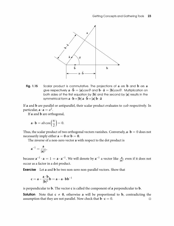
Getting Concepts and Gathering Tools 23
Fig. 1.15 Scalar product is commutative. The projections of a on b and b on agive respectively a · b = |a|cosθ and b · a = |b|cosθ. Multiplication onboth sides of the first equation by |b| and the second by |a| results in thesymmetrical form a ·b = |b| a · b = |a| b · a
If a and b are parallel or antiparallel, their scalar product evaluates to ±ab respectively. Inparticular, a · a = a2.
If a and b are orthogonal,
a ·b = abcos(π
2
)= 0.
Thus, the scalar product of two orthogonal vectors vanishes. Conversely, a ·b = 0 does notnecessarily imply either a = 0 or b = 0.
The inverse of a non-zero vector a with respect to the dot product is
a−1 =a|a|2
,
because a−1 · a = 1 = a · a−1. We will denote by a−1 a vector like a|a|2 even if it does not
occur as a factor in a dot product.
Exercise Let a and b be two non-zero non-parallel vectors. Show that
c = a− a ·b|b|2
b = a− a ·bb−1
is perpendicular to b. The vector c is called the component of a perpendicular to b.
Solution Note that c , 0, otherwise a will be proportional to b, contradicting theassumption that they are not parallel. Now check that b · c = 0.
24 An Introduction to Vectors, Vector Operators and Vector Analysis
If i1, i2, i3 is an orthonormal basis, then
ik · il = δkl ; k, l = 1,2,3 (1.5)
where δkl is the Kronecker delta, whose value is 1 if k = l and zero if k , l.Consider a vector v and a orthonormal basis i, j, k so that
v = vx i+ vy j+ vzk. (1.6)
Dotting both sides with i, j, k successively and using orthonormality of the basis (Eq.(1.5)), we get,
vs = v · n ; s = x,y,z ; n = i, j, k. (1.7)
Thus, coordinates of v along x, y, z axes (namely vx,vy ,vz) are given by its projections onthese axes. If we put v = 0 in Eq. (1.6), by Eq. (1.7) we get vs = 0; s = x,y,z. This meansthat any orthogonal triplet of vectors is linearly independent.
Exercise Show that n > 1 mutually orthogonal non-zero vectors are linearlyindependent.
Solution Let ek , k = 1, . . . ,n be mutually orthogonal non-zero vectors, so that
ei · ej = δij |ej |2,
where δij is the Kronecker delta. Consider the equation
α1e1 +α2e2 + · · ·+αnen = 0
and take its scalar product successively with ei , i = 1, . . . ,n to get αi = 0, i = 1, . . . ,n.Note that the converse is not true. We conclude that any four or more vectors in E3 cannotbe mutually perpendicular.
Direction cosines
Given a vector v and an orthonormal basis i1, i2, i3 we define the quantities
ξk =v · ik||v||
=vk||v||
= v · ik , k = 1,2,3.
If α1,α2,α3 are the angles made by the direction of v with i1, i2, i3 respectively, then
ξk = cosαk , k = 1,2,3.
ξk are called the direction cosines of the vector v with respect to the orthonormal basisi1, i2, i3. Direction cosines unambiguously specify the direction of a non-zero vector. Inparticular, two or more vectors having the same direction cosines with respect to someorthonormal basis have the same directions. The only vector with all the direction cosines
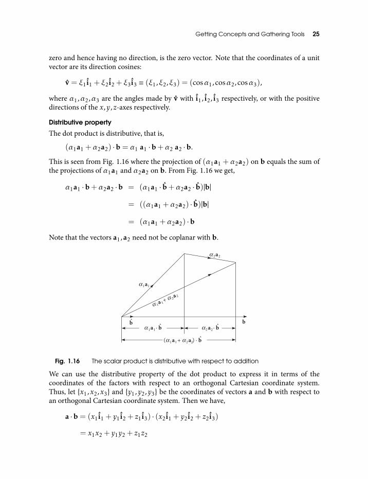
Getting Concepts and Gathering Tools 25
zero and hence having no direction, is the zero vector. Note that the coordinates of a unitvector are its direction cosines:
v = ξ1i1 + ξ2i2 + ξ3i3 ≡ (ξ1,ξ2,ξ3) = (cosα1, cosα2, cosα3),
where α1,α2,α3 are the angles made by v with i1, i2, i3 respectively, or with the positivedirections of the x,y,z-axes respectively.
Distributive property
The dot product is distributive, that is,
(α1a1 +α2a2) ·b = α1 a1 ·b+α2 a2 ·b.
This is seen from Fig. 1.16 where the projection of (α1a1 +α2a2) on b equals the sum ofthe projections of α1a1 and α2a2 on b. From Fig. 1.16 we get,
α1a1 ·b+α2a2 ·b = (α1a1 · b+α2a2 · b)|b|
= ((α1a1 +α2a2) · b)|b|
= (α1a1 +α2a2) ·b
Note that the vectors a1,a2 need not be coplanar with b.
Fig. 1.16 The scalar product is distributive with respect to addition
We can use the distributive property of the dot product to express it in terms of thecoordinates of the factors with respect to an orthogonal Cartesian coordinate system.Thus, let x1,x2,x3 and y1,y2,y3 be the coordinates of vectors a and b with respect toan orthogonal Cartesian coordinate system. Then we have,
a ·b = (x1i1 + y1i2 + z1i3) · (x2i1 + y2i2 + z2i3)
= x1x2 + y1y2 + z1z2
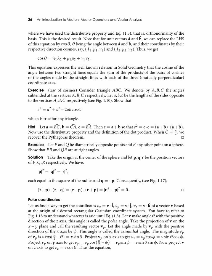
26 An Introduction to Vectors, Vector Operators and Vector Analysis
where we have used the distributive property and Eq. (1.5), that is, orthonormality of thebasis. This is the desired result. Note that for unit vectors a and b, we can replace the LHSof this equation by cosθ, θ being the angle between a and b, and their coordinates by theirrespective direction cosines, say, (λ1,µ1,ν1) and (λ2,µ2,ν2). Thus, we get
cosθ = λ1λ2 + µ1µ2 + ν1ν2.
This equation expresses the well known relation in Solid Geometry that the cosine of theangle between two straight lines equals the sum of the products of the pairs of cosinesof the angles made by the straight lines with each of the three (mutually perpendicular)coordinate axes.
Exercise (law of cosines) Consider triangle ABC. We denote by A,B,C the anglessubtended at the vertices A,B,C respectively. Let a,b,c be the lengths of the sides oppositeto the vertices A,B,C respectively (see Fig. 1.10). Show that
c2 = a2 + b2 − 2abcosC.
which is true for any triangle.
Hint Let a = ~BC, b = ~CA, c = ~BA. Then c = a+b so that c2 = c ·c = (a+b) ·(a+b).Now use the distributive property and the definition of the dot product. When C = π
2 , werecover the Pythagoras theorem.
Exercise Let P andQ be diametrically opposite points andR any other point on a sphere.Show that P R andQR are at right angles.
Solution Take the origin at the center of the sphere and let p,q,r be the position vectorsof P ,Q,R respectively. We have,
|p|2 = |q|2 = |r|2,
each equal to the square of the radius and q = −p. Consequently, (see Fig. 1.17),
(r−p) · (r−q) = (r−p) · (r+p) = |r|2 − |p|2 = 0.
Polar coordinates
Let us find a way to get the coordinates vx = v · i, vy = v · j, vz = v · k of a vector v basedat the origin of a dextral rectangular Cartesian coordinate system. You have to refer toFig. 1.18 to understand whatever is said until Eq. (1.8). Let v make angle θ with the positivedirection of the z axis. this angle is called the polar angle. Take the projection of v on thex − y plane and call the resulting vector vp. Let the angle made by vp with the positivedirection of the x axis be φ. This angle is called the azimuthal angle. The magnitude vpof vp is v cos(π2 −θ) = v sinθ. Project vp on x axis to get vx = vp cosφ = v sinθ cosφ.Project vp on y axis to get vy = vp cos(π2 −φ) = vp sinφ = v sinθ sinφ. Now project von z axis to get vz = v cosθ. Thus the equation,
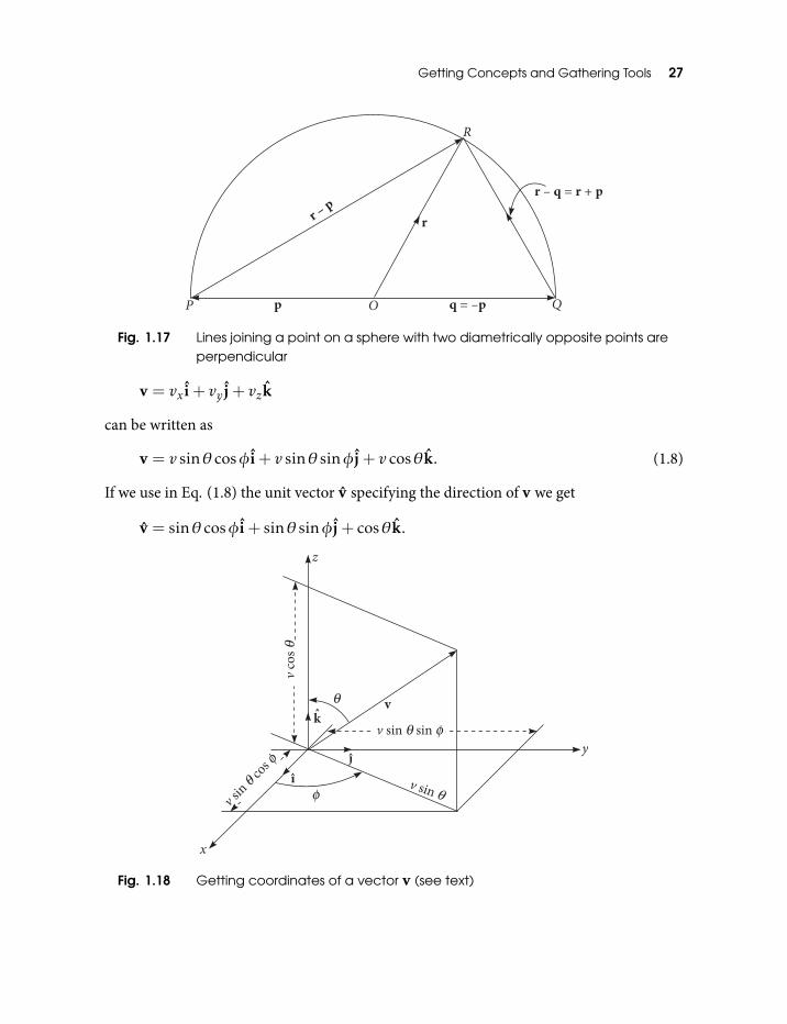
Getting Concepts and Gathering Tools 27
Fig. 1.17 Lines joining a point on a sphere with two diametrically opposite points areperpendicular
v = vx i+ vy j+ vzk
can be written as
v = v sinθ cosφi+ v sinθ sinφj+ v cosθk. (1.8)
If we use in Eq. (1.8) the unit vector v specifying the direction of v we get
v = sinθ cosφi+ sinθ sinφj+ cosθk.
Fig. 1.18 Getting coordinates of a vector v (see text)
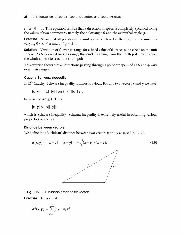
28 An Introduction to Vectors, Vector Operators and Vector Analysis
since |v| = 1. This equation tells us that a direction in space is completely specified fixingthe values of two parameters, namely, the polar angle θ and the azimuthal angle φ.
Exercise Show that all points on the unit sphere centered at the origin are scanned byvarying 0 ≤ θ ≤ π and 0 ≤ φ < 2π.
Solution Variation of φ over its range for a fixed value of θ traces out a circle on the unitsphere. As θ is varied over its range, this circle, starting from the north pole, moves overthe whole sphere to reach the south pole.
This exercise shows that all directions passing through a point are spanned as θ andφ varyover their ranges.
Cauchy–Schwarz inequality
In R3 Cauchy–Schwarz inequality is almost obvious. For any two vectors x and y we have
|x · y|= ||x|| ||y|| |cosθ| ≤ ||x|| ||y||.
because |cosθ| ≤ 1. Thus,
|x · y| ≤ ||x|| ||y||,
which is Schwarz Inequality. Schwarz inequality is extremely useful in obtaining variousproperties of vectors.
Distance between vectors
We define the (Euclidean) distance between two vectors x and y as (see Fig. 1.19),
d(x,y) = ||x− y||= |x− y|= +√(x− y) · (x− y). (1.9)
Fig. 1.19 Euclidean distance for vectors
Exercise Check that
d2(x,y) =3∑k=1
(xk − yk)2,
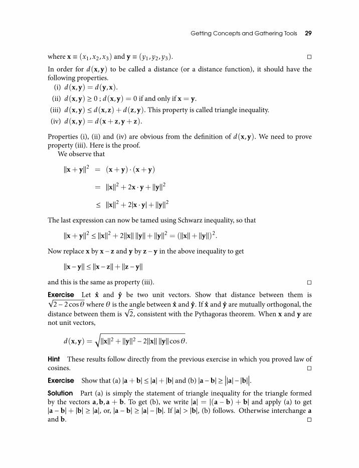
Getting Concepts and Gathering Tools 29
where x ≡ (x1,x2,x3) and y ≡ (y1,y2,y3).
In order for d(x,y) to be called a distance (or a distance function), it should have thefollowing properties.
(i) d(x,y) = d(y,x).
(ii) d(x,y) ≥ 0 ; d(x,y) = 0 if and only if x = y.
(iii) d(x,y) ≤ d(x,z) + d(z,y). This property is called triangle inequality.(iv) d(x,y) = d(x+ z,y+ z).
Properties (i), (ii) and (iv) are obvious from the definition of d(x,y). We need to proveproperty (iii). Here is the proof.
We observe that
||x+ y||2 = (x+ y) · (x+ y)
= ||x||2 + 2x · y+ ||y||2
≤ ||x||2 + 2|x · y|+ ||y||2
The last expression can now be tamed using Schwarz inequality, so that
||x+ y||2 ≤ ||x||2 + 2||x|| ||y||+ ||y||2 = (||x||+ ||y||)2.
Now replace x by x− z and y by z− y in the above inequality to get
||x− y|| ≤ ||x− z||+ ||z− y||
and this is the same as property (iii).
Exercise Let x and y be two unit vectors. Show that distance between them is√2− 2cosθ where θ is the angle between x and y. If x and y are mutually orthogonal, the
distance between them is√
2, consistent with the Pythagoras theorem. When x and y arenot unit vectors,
d(x,y) =√||x||2 + ||y||2 − 2||x|| ||y||cosθ.
Hint These results follow directly from the previous exercise in which you proved law ofcosines.
Exercise Show that (a) |a+b| ≤ |a|+ |b| and (b) |a−b| ≥∣∣∣|a| − |b|∣∣∣.
Solution Part (a) is simply the statement of triangle inequality for the triangle formedby the vectors a,b,a + b. To get (b), we write |a| = |(a − b) + b| and apply (a) to get|a − b|+ |b| ≥ |a|, or, |a − b| ≥ |a| − |b|. If |a| > |b|, (b) follows. Otherwise interchange aand b.
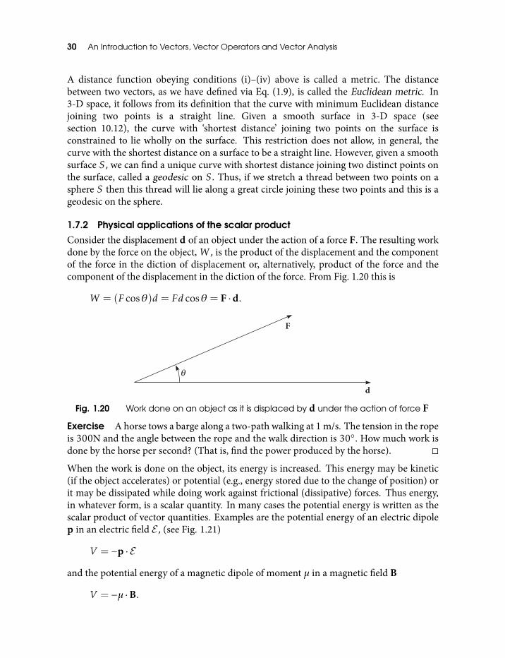
30 An Introduction to Vectors, Vector Operators and Vector Analysis
A distance function obeying conditions (i)–(iv) above is called a metric. The distancebetween two vectors, as we have defined via Eq. (1.9), is called the Euclidean metric. In3-D space, it follows from its definition that the curve with minimum Euclidean distancejoining two points is a straight line. Given a smooth surface in 3-D space (seesection 10.12), the curve with ‘shortest distance’ joining two points on the surface isconstrained to lie wholly on the surface. This restriction does not allow, in general, thecurve with the shortest distance on a surface to be a straight line. However, given a smoothsurface S, we can find a unique curve with shortest distance joining two distinct points onthe surface, called a geodesic on S. Thus, if we stretch a thread between two points on asphere S then this thread will lie along a great circle joining these two points and this is ageodesic on the sphere.
1.7.2 Physical applications of the scalar product
Consider the displacement d of an object under the action of a force F. The resulting workdone by the force on the object, W , is the product of the displacement and the componentof the force in the diction of displacement or, alternatively, product of the force and thecomponent of the displacement in the diction of the force. From Fig. 1.20 this is
W = (F cosθ)d = Fd cosθ = F ·d.
Fig. 1.20 Work done on an object as it is displaced by d under the action of force F
Exercise A horse tows a barge along a two-path walking at 1 m/s. The tension in the ropeis 300N and the angle between the rope and the walk direction is 30. How much work isdone by the horse per second? (That is, find the power produced by the horse).
When the work is done on the object, its energy is increased. This energy may be kinetic(if the object accelerates) or potential (e.g., energy stored due to the change of position) orit may be dissipated while doing work against frictional (dissipative) forces. Thus energy,in whatever form, is a scalar quantity. In many cases the potential energy is written as thescalar product of vector quantities. Examples are the potential energy of an electric dipolep in an electric field E, (see Fig. 1.21)
V = −p · E
and the potential energy of a magnetic dipole of moment µ in a magnetic field B
V = −µ ·B.
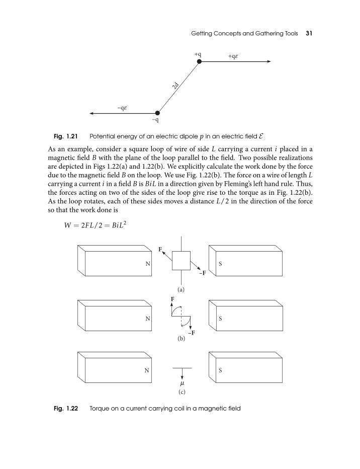
Getting Concepts and Gathering Tools 31
Fig. 1.21 Potential energy of an electric dipole p in an electric field E
As an example, consider a square loop of wire of side L carrying a current i placed in amagnetic field B with the plane of the loop parallel to the field. Two possible realizationsare depicted in Figs 1.22(a) and 1.22(b). We explicitly calculate the work done by the forcedue to the magnetic field B on the loop. We use Fig. 1.22(b). The force on a wire of length Lcarrying a current i in a field B is BiL in a direction given by Fleming’s left hand rule. Thus,the forces acting on two of the sides of the loop give rise to the torque as in Fig. 1.22(b).As the loop rotates, each of these sides moves a distance L/2 in the direction of the forceso that the work done is
W = 2FL/2 = BiL2
Fig. 1.22 Torque on a current carrying coil in a magnetic field
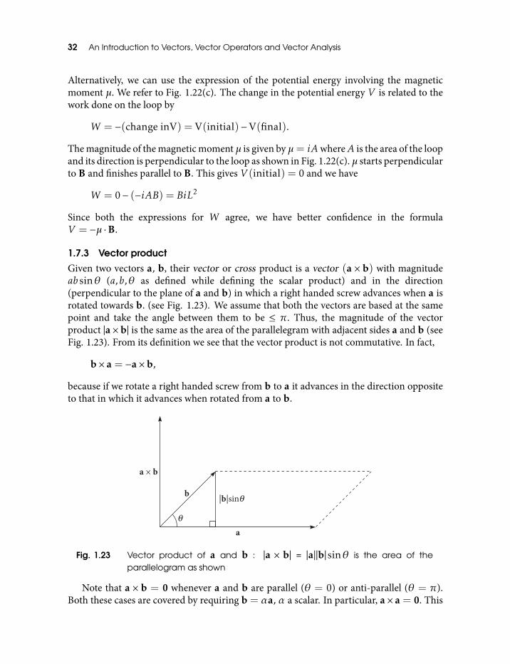
32 An Introduction to Vectors, Vector Operators and Vector Analysis
Alternatively, we can use the expression of the potential energy involving the magneticmoment µ. We refer to Fig. 1.22(c). The change in the potential energy V is related to thework done on the loop by
W = −(change inV) = V(initial)−V(final).
The magnitude of the magnetic moment µ is given by µ= iAwhereA is the area of the loopand its direction is perpendicular to the loop as shown in Fig. 1.22(c).µ starts perpendicularto B and finishes parallel to B. This gives V (initial) = 0 and we have
W = 0− (−iAB) = BiL2
Since both the expressions for W agree, we have better confidence in the formulaV = −µ ·B.
1.7.3 Vector product
Given two vectors a, b, their vector or cross product is a vector (a × b) with magnitudeab sinθ (a,b,θ as defined while defining the scalar product) and in the direction(perpendicular to the plane of a and b) in which a right handed screw advances when a isrotated towards b. (see Fig. 1.23). We assume that both the vectors are based at the samepoint and take the angle between them to be ≤ π. Thus, the magnitude of the vectorproduct |a×b| is the same as the area of the parallelegram with adjacent sides a and b (seeFig. 1.23). From its definition we see that the vector product is not commutative. In fact,
b× a = −a×b,
because if we rotate a right handed screw from b to a it advances in the direction oppositeto that in which it advances when rotated from a to b.
Fig. 1.23 Vector product of a and b : |a × b| = |a||b|sinθ is the area of theparallelogram as shown
Note that a × b = 0 whenever a and b are parallel (θ = 0) or anti-parallel (θ = π).Both these cases are covered by requiring b = αa, α a scalar. In particular, a× a = 0. This
Getting Concepts and Gathering Tools 33
shows that a×b = 0 if and only if a , 0 and b , 0 are proportional to each other, that is,are linearly dependent.
The vector product is not associative as can be seen from
(a× a)×b , a× (a×b)
with a , 0,b , 0, as the LHS is always zero, while RHS is never zero unless b = αa. RHSis a vector in the plane of a, b with magnitude a2b sinθ (θ : angle between a and b).
The vector product is distributive, that is,
a× (b+ c) = a×b+ a× c,
and (a+b)× c = a× c+b× c.
We will prove this result later (see subsection 1.8.1).From its definition, it follows that multiplying one of the factors of a vector product by
a scalar amounts to multiplying the vector product itself by that scalar.All of the above discussion leads immediately to the laws of vector multiplication:
(λa)×b = a× (λb) = λ(a×b)
a× (b+ c) = a×b+ a× c
(a+b)× c = a× c+b× c
b× a = −a×b. (1.10)
Exercise Show that (a) (a·b)2+(a×b)2 = a2b2 and (b) (a·b)2−(a×b)2 = a2b2 cos2θwhere θ is the angle between a and b. Part (a) immediately leads to Cauchy–Schwartzinequality,
|a ·b| ≤ |a| |b|
with an additional piece of information that equality holds if and only if the vectors a andb are linearly dependent.
Exercise If a⊥ and b⊥ are the components of a and b perpendicular to a vector c thenshow that (a) a× c = a⊥ × c and (b) (a+b)× c = (a⊥+b⊥)× c.
Solution Note that c, a and a⊥ are coplanar with a and a⊥ on the same side of c (Draw afigure) and a⊥×c and a×c have the same direction. Let θ be the angle between a and c andlet the angle between a and a⊥ be φ. Note that θ+φ = π
2 . Therefore, for the magnitudes,we get
a⊥ = acosφ = asinθ,
34 An Introduction to Vectors, Vector Operators and Vector Analysis
leading to |a × c| = |a⊥ × c| so that (a) is proved. To get (b), note that a⊥ + b⊥ is thecomponent of a+b perpendicular to c and apply (a).
Consider an orthonormal basis i, j, k forming a right handed coordinate system. Fromthe definitions of the vector product and a right handed coordinate system it immediatelyfollows that
i× i = j× j = k× k = 0
and
i× j = −j× i = k
j× k = −k× j = i
k× i = −i× k = j. (1.11)
Note that we can obtain the second and the third equation above from the first by cyclicallypermuting the vectors i, j, k. i.e., by simultaneously changing i 7→ j, j 7→ k, k 7→ i. Thisuseful property holds for any vector relation involving an orthonormal basis.
For a left handed coordinate system the vectors i× j, j× k, k× i are in opposite directionto the basis vectors k, i, j respectively. Therefore, Eq. (1.11) change to
i× j = −k
j× k = −i
k× i = −j. (1.12)
Equations (1.11) and (1.12) are often taken to be the definitions of the right handed andthe left handed coordinate systems respectively.
Exercise Prove that
a×b =
∣∣∣∣∣∣a2 b2
a3 b3
∣∣∣∣∣∣ σ1 −∣∣∣∣∣∣a1 b1
a3 b3
∣∣∣∣∣∣ σ2 +
∣∣∣∣∣∣a1 b1
a2 b2
∣∣∣∣∣∣ σ3,
σ1, σ2, σ3 is an orthonormal right handed basis and ak = a · σk , bk = b · σk , k = 1,2,3.
Exercise Compute (a) (a + b) × (a − b); (b) (a − b) × (b − c). Give a geometricalinterpretation of these.
Hint Think of a tetrahedron.
Getting Concepts and Gathering Tools 35
Exercise If (a × b) = (c × d) and (a × c) = (b × d) then show that a − d is parallel tob− c.
Hint Subtract these two equations.
Using the distributive property of the vector product and Eq. (1.11) we can write thevector product of two vectors in terms of their Cartesian components with respect to aright handed coordinate system.
a×b = (ax i+ ay j+ azk)× (bx i+ by j+ bzk)
= (aybz − byaz)i+ (azbx − bzax)j+ (axby − bxay)k. (1.13)
This expression for the vector product in component form contains no easily accessibleinformation about the magnitude and the direction of the vector product a × b. Also, itdepends on the coordinate system used as the components of the factors change if we useanother orthonormal basis, (that is, another coordinate system). On the other hand,expressions involving vectors (and not their components) are invariant under the changeof coordinate system and each term in them has the same value in all coordinate systems.Thus, if we can model a physical situation or a process using vectors and expressionsinvolving vectors alone, we are free of the limitation of viewing the process with referenceto a particular coordinate system and of extra baggage of transforming the expressionsfrom one coordinate system to the other as and when required. The most importantadvantage of vectors is this coordinate-free approach they offer. In this book we willexclusively follow this coordinate-free approach, although we will spend some time withsome of the important coordinate systems.
The components of a × b with respect to an orthonormal basis i, j, k (and thecorresponding coordinate system) can be expressed more conveniently in the form∣∣∣∣∣∣∣∣∣
i j kax ay azbx by bz
∣∣∣∣∣∣∣∣∣ ·Exercise (Law of sines) Refer to the exercise where you are asked to prove law of cosinesfor a triangle ABC and Fig. 1.10. Prove Eq. (1.14).
Solution Take the vector product of c = a+b successively with vectors a,b,c to get
a× c = a×b = c×b.
Equating the magnitudes of these vectors and dividing by abc gives a relation true for anytriangle,
sinAa
=sinBb
=sinCc
. (1.14)
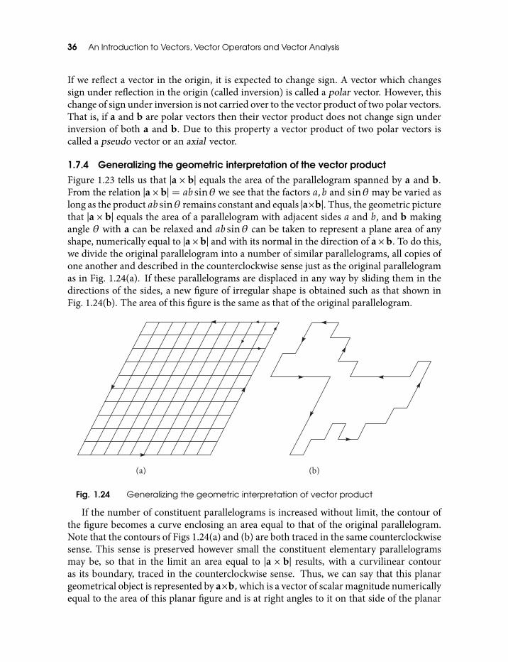
36 An Introduction to Vectors, Vector Operators and Vector Analysis
If we reflect a vector in the origin, it is expected to change sign. A vector which changessign under reflection in the origin (called inversion) is called a polar vector. However, thischange of sign under inversion is not carried over to the vector product of two polar vectors.That is, if a and b are polar vectors then their vector product does not change sign underinversion of both a and b. Due to this property a vector product of two polar vectors iscalled a pseudo vector or an axial vector.
1.7.4 Generalizing the geometric interpretation of the vector product
Figure 1.23 tells us that |a × b| equals the area of the parallelogram spanned by a and b.From the relation |a×b| = ab sinθ we see that the factors a,b and sinθ may be varied aslong as the product ab sinθ remains constant and equals |a×b|. Thus, the geometric picturethat |a × b| equals the area of a parallelogram with adjacent sides a and b, and b makingangle θ with a can be relaxed and ab sinθ can be taken to represent a plane area of anyshape, numerically equal to |a×b| and with its normal in the direction of a×b. To do this,we divide the original parallelogram into a number of similar parallelograms, all copies ofone another and described in the counterclockwise sense just as the original parallelogramas in Fig. 1.24(a). If these parallelograms are displaced in any way by sliding them in thedirections of the sides, a new figure of irregular shape is obtained such as that shown inFig. 1.24(b). The area of this figure is the same as that of the original parallelogram.
Fig. 1.24 Generalizing the geometric interpretation of vector product
If the number of constituent parallelograms is increased without limit, the contour ofthe figure becomes a curve enclosing an area equal to that of the original parallelogram.Note that the contours of Figs 1.24(a) and (b) are both traced in the same counterclockwisesense. This sense is preserved however small the constituent elementary parallelogramsmay be, so that in the limit an area equal to |a × b| results, with a curvilinear contouras its boundary, traced in the counterclockwise sense. Thus, we can say that this planargeometrical object is represented by a×b, which is a vector of scalar magnitude numericallyequal to the area of this planar figure and is at right angles to it on that side of the planar
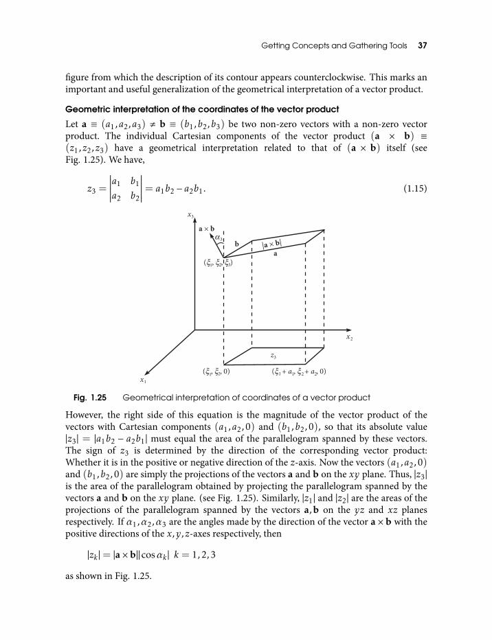
Getting Concepts and Gathering Tools 37
figure from which the description of its contour appears counterclockwise. This marks animportant and useful generalization of the geometrical interpretation of a vector product.
Geometric interpretation of the coordinates of the vector product
Let a ≡ (a1,a2,a3) , b ≡ (b1,b2,b3) be two non-zero vectors with a non-zero vectorproduct. The individual Cartesian components of the vector product (a × b) ≡(z1,z2,z3) have a geometrical interpretation related to that of (a × b) itself (seeFig. 1.25). We have,
z3 =
∣∣∣∣∣∣a1 b1
a2 b2
∣∣∣∣∣∣= a1b2 − a2b1. (1.15)
Fig. 1.25 Geometrical interpretation of coordinates of a vector product
However, the right side of this equation is the magnitude of the vector product of thevectors with Cartesian components (a1,a2,0) and (b1,b2,0), so that its absolute value|z3| = |a1b2 − a2b1| must equal the area of the parallelogram spanned by these vectors.The sign of z3 is determined by the direction of the corresponding vector product:Whether it is in the positive or negative direction of the z-axis. Now the vectors (a1,a2,0)and (b1,b2,0) are simply the projections of the vectors a and b on the xy plane. Thus, |z3|is the area of the parallelogram obtained by projecting the parallelogram spanned by thevectors a and b on the xy plane. (see Fig. 1.25). Similarly, |z1| and |z2| are the areas of theprojections of the parallelogram spanned by the vectors a,b on the yz and xz planesrespectively. If α1,α2,α3 are the angles made by the direction of the vector a×b with thepositive directions of the x,y,z-axes respectively, then
|zk |= |a×b||cosαk | k = 1,2,3
as shown in Fig. 1.25.
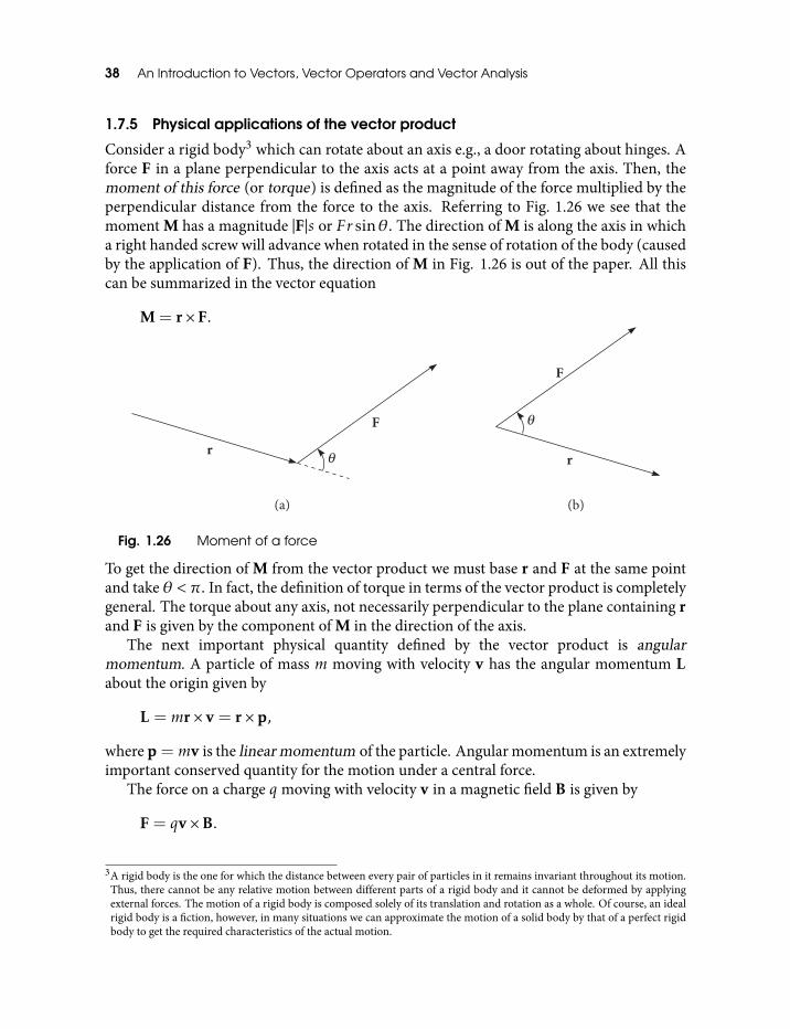
38 An Introduction to Vectors, Vector Operators and Vector Analysis
1.7.5 Physical applications of the vector product
Consider a rigid body3 which can rotate about an axis e.g., a door rotating about hinges. Aforce F in a plane perpendicular to the axis acts at a point away from the axis. Then, themoment of this force (or torque) is defined as the magnitude of the force multiplied by theperpendicular distance from the force to the axis. Referring to Fig. 1.26 we see that themoment M has a magnitude |F|s or Fr sinθ. The direction of M is along the axis in whicha right handed screw will advance when rotated in the sense of rotation of the body (causedby the application of F). Thus, the direction of M in Fig. 1.26 is out of the paper. All thiscan be summarized in the vector equation
M = r×F.
Fig. 1.26 Moment of a force
To get the direction of M from the vector product we must base r and F at the same pointand take θ < π. In fact, the definition of torque in terms of the vector product is completelygeneral. The torque about any axis, not necessarily perpendicular to the plane containing rand F is given by the component of M in the direction of the axis.
The next important physical quantity defined by the vector product is angularmomentum. A particle of mass m moving with velocity v has the angular momentum Labout the origin given by
L =mr× v = r×p,
where p =mv is the linear momentum of the particle. Angular momentum is an extremelyimportant conserved quantity for the motion under a central force.
The force on a charge q moving with velocity v in a magnetic field B is given by
F = qv×B.
3A rigid body is the one for which the distance between every pair of particles in it remains invariant throughout its motion.Thus, there cannot be any relative motion between different parts of a rigid body and it cannot be deformed by applyingexternal forces. The motion of a rigid body is composed solely of its translation and rotation as a whole. Of course, an idealrigid body is a fiction, however, in many situations we can approximate the motion of a solid body by that of a perfect rigidbody to get the required characteristics of the actual motion.
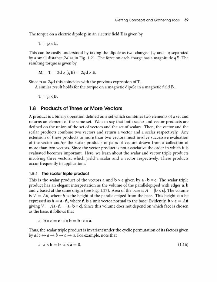
Getting Concepts and Gathering Tools 39
The torque on a electric dipole p in an electric field E is given by
T = p×E.
This can be easily understood by taking the dipole as two charges +q and −q separatedby a small distance 2d as in Fig. 1.21. The force on each charge has a magnitude qE. Theresulting torque is given by
M = T = 2d× (qE) = 2qd×E.
Since p = 2qd this coincides with the previous expression of T.A similar result holds for the torque on a magnetic dipole in a magnetic field B.
T = µ×B.
1.8 Products of Three or More VectorsA product is a binary operation defined on a set which combines two elements of a set andreturns an element of the same set. We can say that both scalar and vector products aredefined on the union of the set of vectors and the set of scalars. Then, the vector and thescalar products combine two vectors and return a vector and a scalar respectively. Anyextension of these products to more than two vectors must involve successive evaluationof the vector and/or the scalar products of pairs of vectors drawn from a collection ofmore than two vectors. Since the vector product is not associative the order in which it isevaluated becomes important. Here, we learn about the scalar and vector triple productsinvolving three vectors, which yield a scalar and a vector respectively. These productsoccur frequently in applications.
1.8.1 The scalar triple product
This is the scalar product of the vectors a and b × c given by a · b × c. The scalar tripleproduct has an elegant interpretation as the volume of the parallelepiped with edges a,band c based at the same origin (see Fig. 1.27). Area of the base is A = |b× c|. The volumeis V = Ah, where h is the height of the parallelepiped from the base. This height can beexpressed as h = a · n, where n is a unit vector normal to the base. Evidently, b× c = Angiving V = Aa · n = |a ·b× c|. Since this volume does not depend on which face is chosenas the base, it follows that
a ·b× c = c · a×b = b · c× a.
Thus, the scalar triple product is invariant under the cyclic permutation of its factors givenby abc↔ a→ b→ c→ a. For example, note that
a · a×b = b · a× a = 0. (1.16)
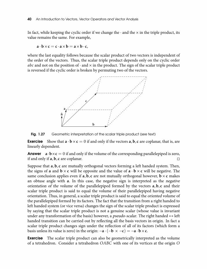
40 An Introduction to Vectors, Vector Operators and Vector Analysis
In fact, while keeping the cyclic order if we change the · and the × in the triple product, itsvalue remains the same. For example,
a ·b× c = c · a×b = a×b · c,
where the last equality follows because the scalar product of two vectors is independent ofthe order of the vectors. Thus, the scalar triple product depends only on the cyclic orderabc and not on the position of · and × in the product. The sign of the scalar triple productis reversed if the cyclic order is broken by permuting two of the vectors.
Fig. 1.27 Geometric interpretation of the scalar triple product (see text)
Exercise Show that a ·b× c = 0 if and only if the vectors a,b,c are coplanar, that is, arelinearly dependent.
Answer a ·b×c = 0 if and only if the volume of the corresponding parallelepiped is zero,if and only if a,b,c are coplanar.
Suppose that a,b,c are mutually orthogonal vectors forming a left handed system. Then,the signs of a and b × c will be opposite and the value of a · b × c will be negative. Thesame conclusion applies even if a,b,c are not mutually orthogonal however, b × c makesan obtuse angle with a. In this case, the negative sign is interpreted as the negativeorientation of the volume of the parallelepiped formed by the vectors a,b,c and theirscalar triple product is said to equal the volume of their parallelepiped having negativeorientation. Thus, in general, a scalar triple product is said to equal the oriented volume ofthe parallelepiped formed by its factors. The fact that the transition from a right handed toleft handed system (or vice versa) changes the sign of the scalar triple product is expressedby saying that the scalar triple product is not a genuine scalar (whose value is invariantunder any transformation of the basis) however, a pseudo-scalar. The right handed↔ lefthanded transition can be carried out by reflecting all the basis vectors in origin. In fact ascalar triple product changes sign under the reflection of all of its factors (which form abasis unless its value is zero) in the origin: −a · (−b × −c) = −a ·b× c.
Exercise The scalar triple product can also be geometrically interpreted as the volumeof a tetrahedron. Consider a tetrahedron OABC with one of its vertices at the origin O
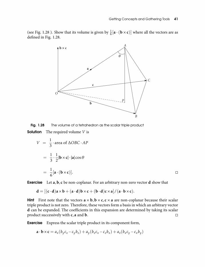
Getting Concepts and Gathering Tools 41
(see Fig. 1.28 ). Show that its volume is given by 16 [a · (b × c)] where all the vectors are as
defined in Fig. 1.28.
Fig. 1.28 The volume of a tetrahedron as the scalar triple product
Solution The required volume V is
V =13· area of ∆OBC ·AP
=13· 1
2|b× c| · |a|cosθ
=16[a · (b× c)].
Exercise Let a,b,c be non-coplanar. For an arbitrary non-zero vector d show that
d = [(c ·d)a×b+ (a ·d)b× c+ (b ·d)c× a]/(a ·b× c).
Hint First note that the vectors a × b,b × c,c × a are non-coplanar because their scalartriple product is not zero. Therefore, these vectors form a basis in which an arbitrary vectord can be expanded. The coefficients in this expansion are determined by taking its scalarproduct successively with c,a and b.
Exercise Express the scalar triple product in its component form,
a ·b× c = ax(bycz − cybz) + ay(bzcx − czbx) + az(bxcy − cxby)
42 An Introduction to Vectors, Vector Operators and Vector Analysis
and write it in the determinant form
a · (b× c) =
∣∣∣∣∣∣∣∣∣ax ay azbx by bzcx cy cz
∣∣∣∣∣∣∣∣∣= det(a,b,c),
which defines det(a,b,c).4
Hint Use Eq. (1.13) for the vector product.
Exercise Let θ be the angle between the directions of vectors c and a×b. Show that
det(a,b,c) = |a×b| |c|cosθ.
Exercise Show that the area of the parallelogram spanned by a,b, namely, |a×b|, can beexpressed by
|a×b|2 = (a · a)(b ·b)− (a ·b)(b · a) =∣∣∣∣∣∣a · a a ·bb · a b ·b
∣∣∣∣∣∣ · (1.17)
This determinant is called Gram determinant . Since |a × b| = 0 if and only if a,b aredependent, we see that the gram determinant is zero if and only if a,b are dependent.
Exercise Show that the determinant form of [a · (b× c)][d · (e× f)] is
[a · (b× c)][d · (e× f)] ≡
∣∣∣∣∣∣∣∣∣a ·d a · e a · fb ·d b · e b · fc ·d c · e c · f
∣∣∣∣∣∣∣∣∣ ·Hint Treat the rows and columns forming the determinants of factors as matrices, andfind the determinant of the product of matrix of one factor and the transpose of the matrixof the other factor. This works because the determinant of the product of matrices is theproduct of their determinants and the determinant of a matrix is invariant under transposeof that matrix.
Let us now prove that the vector product is distributive. Let a,b,c be three arbitraryvectors and let x be an arbitrary direction. Using the fact that the scalar triple product isinvariant under the cyclic permutation of its factors, we can write
x · a× (b+ c) = (b+ c) · (x× a)
= b · (x× a) + c · (x× a)
= x · (a×b+ a× c)
4You are now advised to read the appendix on matrices and determinants, which will be used in the rest of the book.
Getting Concepts and Gathering Tools 43
Since x is arbitrary, we get
a× (b+ c) = a×b+ a× c,
which is the desired result.The distributive law
(a+b)× c = a× c+b× c
can be proved similarly.A powerful notation for the scalar triple product a·(b×c) and all its cyclic permutations
is [abc]. This notation was first used by Grassmann. However, we will use this notation veryrarely and prefer to write scalar triple product explicitly.
1.8.2 Physical applications of the scalar triple product
Reciprocal lattice of a crystal [4].A single crystal is characterized by the periodic arrangement of atoms, ions or
molecules. This periodic arrangement is modelled by a lattice of points in space, called aBravais lattice. Since a crystal is a three dimensional object, we expect the lattice to havethree independent periodic arrangements in three non-coplanar directions. We canimagine three basis vectors (called primitive vectors) say a1,a2,a3 along threenon-coplanar directions forming the adjacent edges of a parallelepiped which is called aprimitive cell of the Bravais lattice. The Bravais lattice can be constructed by translatingthis primitive cell integral number of times successively along the directions defined by theprimitive vectors a1,a2,a3. Obviously, only those primitive cells are allowed which fill inall the space by such a translation. A vector joining the origin to any of the lattice points,say R, is then given by
R = n1a1 + n2a2 + n3a3
where n1,n2,n3 are integers. The whole lattice is given by the set of vectors Rgenerated by giving the triplet n1,n2,n3 all possible integer values. Note that the volumeof a primitive cell is given by the scalar triple product a1 · a2 × a3 or any of its cyclicpermutations.
Consider a set of points R constituting the Bravais lattice of a crystal in which a planewave eik·r is excited. Here, k is a wave vector and r is an arbitrary point in the crystal. Weseek to find the set of wave vectors K for which the plane wave excitation has the sameperiodicity as the Bravais lattice of the crystal, that is,
eiK·(r+R) = eiK·r,
which means
eiK·R = 1 (1.18)
44 An Introduction to Vectors, Vector Operators and Vector Analysis
for all R in the Bravais lattice. The set of vectors K satisfying Eq. (1.18) is called thereciprocal lattice of the given Bravais lattice. The corresponding Bravais lattice is called thedirect lattice .
If K1,K2 satisfy Eq. (1.18), then so do their sum and difference, which simply meansthat the set of reciprocal vectors form a Bravais lattice. We show that the primitive vectorsof the reciprocal lattice are given by
b1 = 2πa2 × a3
a1 · a2 × a3,
b2 = 2πa3 × a1
a1 · a2 × a3,
b3 = 2πa1 × a2
a1 · a2 × a3. (1.19)
Exercise Show that ai ·bj = 2πδij where δij = 0,1(i , j, i = j).
Exercise Show that bis are not all in one plane as long as ais are not.
Since bis are non-coplanar, any vector k can be written as a linear combination of bi,
k = k1b1 + k2b2 + k3b3.
If R is any direct lattice vector, then
R = n1a1 + n2a2 + n3a3
where n1,n2,n3 are integers. Since ai ·bj = 2πδij it follows that
k ·R = 2π(k1n1 + k2n2 + k3n3).
We conclude from this equation that eik·R is unity for all R, only when the coefficientsk1,k2,k3 are integers (i.e., when k ·R is an integral multiple of 2π). Thus, we must have,for a reciprocal lattice vector K,
K = k1b1 + k2b2 + k3b3,
where k1,k2,k3 are integers. Thus, reciprocal lattice is a Bravais lattice and bis can betaken to be its primitive vectors. bis form the adjacent sides of a parallelepiped which is theprimitive cell of the reciprocal lattice.
Apart from, an enormous variety of situations in which the scalar triple product makesits appearance, it is an important tool for the development of the theory of vector operators,as we shall see in the next chapter. Also, the scalar triple product is the basis of a new andpowerful notation for vector algebra and calculus, namely the Levi-Civita symbols (seesection 1.11).
Getting Concepts and Gathering Tools 45
1.8.3 The vector triple product
This is the vector product of the vector a with the vector b × c, that is, a × (b × c). Thisvector is in the plane containing vectors b and c because b × c is perpendicular to thisplane and a× (b× c) is perpendicular to b× c. Since the vector product is not associativethe position of the brackets in a×(b×c) is of vital importance. Generally, we do not have todirectly evaluate a vector triple product as it can be transformed into a simpler expressionvia a vector identity (see section 1.12).
1.9 Homomorphism and IsomorphismWe need two algebraic concepts, namely, homomorphism and its special caseisomorphism between two sets, which we now define. Consider two pairs (S1,) and(S2,×), where S1,S2 are sets and ,× are binary operations on S1 and S2 respectively. Weassume that S1,S2 are closed under the corresponding binary operations. Let ϕ : S1 7→ S2be a map from S1 to S2 such that for every a ∈ S1 there is a ϕ(a) ∈ S2. We say that ϕ is ahomomorphism if, for every a,b ∈ S1
ϕ(a b) = ϕ(a)×ϕ(b). (1.20)
In other words, the image of the product of a and b in S1 is the product of their imagesϕ(a) and ϕ(b) in S2.
Example Consider (Z,+) and ((1,−1), ·) where Z is the set of integers and + is theusual addition on it, while · is the usual multiplication on the two element set (1,−1).Define a map ϕ by
ϕ(n) = (−1)n,
that is,
(−1)a+b = (−1)a · (−1)b
which is clearly true.If the map ϕ defining a homomorphism is also one to one and onto, then it is called
isomorphism .
Exercise Show that the set Z2 of integers modulo 2 and ((1,−1), ·) defined above, areisomorphic.
1.10 Isomorphism with R3
Until now we used R3 just as a name for the space we live in and in which all physicalphenomena occur. In this section we give exact definition of R3 and justify using it as aname for our space.
46 An Introduction to Vectors, Vector Operators and Vector Analysis
Let us choose an orthonormal basis i, j, k based at some origin O and thecorresponding Cartesian coordinate system. We now use it to assign the Cartesiancoordinates to all points in space. This procedure assigns a unique triplet of real numbersto every point in space. In fact the set of all triplets of real numbers can be identified withthe set of all points in space. We call this set of triplets R3. Although, R3 stands for the setof all real number triplets, its one to one correspondence with the set of points in realspace justifies naming real space by R3 as we have been doing until now.
We have already established a one to one correspondence between the set of vectors(representations of values of vector quantities in space) and R3, (for a given basis), usingthe fact that every vector can be written as a unique linear combination of the basis vectors(see sections 1.3 and 1.6). Here, we want to show something more. First, we define theaddition in R3 as
(a1,a2,a3) + (b1,b2,b3) = (a1 + b1,a2 + b2,a3 + b3).
Consider two vectors a and b with coordinates a1,a2,a3 and b1,b2,b3 respectively. Thismeans
a = a1i+ a2j+ a3k
b = b1i+ b2j+ b3k.
Using the distributive law for the multiplication of vectors by scalars and the commutativityand the associativity of the vector addition we can write
a+b = (a1 + b1)i+ (a2 + b2)j+ (a3 + b3)k.
Thus, the coordinates of a + b are simply the addition of the coordinates of a and thoseof b. Then, we have the following association.
a ↔ (a1,a2,a3),
b ↔ (b1,b2,b3),
a+b ↔ (a1 + b1,a2 + b2,a3 + b3). (1.21)
Let us define the scalar product in R3 as the product of two 1×3 and 3×1 matrices (a rowvector and a column vector),
[a1a2a3][b1b2b3]T =
∑i
aibi (1.22)
where the superscript T denotes the transpose of a matrix. Thus, we see that thecorrespondence Eq. (1.21) preserves the scalar product of vectors.
Getting Concepts and Gathering Tools 47
Thus, we have a one to one map between the two sets: The set of vectors (whoseelements are the ‘values’ of one or more vector quantities) and R3, (whose elements arethe triplets of real numbers) which preserves the addition on individual sets in the sense ofEq. (1.20). Thus, the one to one map defined by Eq. (1.21) is an isomorphism betweenthese two sets. Two isomorphic sets are algebraically identical and it is enough to studyonly one of them. Even the scalar and vector products can be expressed and processed interms of the components of vectors, which are triplets of real numbers. So you may comeup with the idea that we can just do away with the set of vectors and do everything usingthe set of triplets of real numbers, namely R3. This will free us from dealing with vectorsaltogether. A nice idea, but has the following problem. At the end of section 1.3 we sawthat the one to one correspondence between vectors and R3 depends on the origin and thebasis chosen. There is a different isomorphism for each possible origin and each possiblebasis because a change in the basis/origin changes the coordinates of every vector (seeFig. 1.4). Since there could be uncountably many origins and bases, there are uncountablymany isomorphisms possible between the set of vectors and R3. It is then impossible tokeep track of which isomorphism being used and to transform between these. On theother hand, the coordinate free approach, in which we directly deal with the set of vectors,frees us from this problem of keeping track of bases and transforming between them. Italso enables us to reach conclusions that are independent of any particular basis or thecoordinate system. Thus, coordinate free approach turns out to be more fruitful in manyapplications. On the other hand, an intelligent choice of the coordinate system, basicallyguided by the symmetry in the problem, can drastically reduce the algebra and cansharpen the understanding of the physics of the situation. Therefore, a judicious choicebetween these methods, depending on the problem, turns out to be rewarding.
A set V and the associated set of scalars S, with the operations of addition and scalarmultiplication defined on V , which have all the properties of vector addition and scalarmultiplication as listed in section 1.4, is called a linear space. If, in addition, we define ascalar product and the resulting metric (a distance function giving distance between everypair of elements), then it is called a metric space. Thus, a set of vectors is a metric spacewith a Euclidean metric. Let us call the 3-D space comprising all vectors (that is, all valuesof one or more vector quantities) E3. Both E3 and R3 are metric spaces with Euclideanmetric (see Eq. (1.9) and the exercise following it). If a subset of a metric space is closedunder addition, that is, the addition of every pair of vectors in the subset gives a vectorin the same subset, then such a subset is a metric space in its own right and is called asubspace of the parent metric space. A basis in a subspace can always be extended to thatof the whole space. The dimension of a subspace is always ≤ that of the whole space. Thus,for example, a set of planar vectors (a plane) and a set of vectors on a straight line (a straightline) are the 2-D and 1-D subspaces of E3 (R3) respectively.
Since R3 and E3 are isomorphic linear spaces, they can be used interchangeably in allcontexts. However, we will basically refer to the space E3 as we intend to deal directly withthe vectors, although we will make judicious use of R3 as well (when we operate by matriceson 3-D column vectors comprising the coordinates of vectors, see the next chapter).
48 An Introduction to Vectors, Vector Operators and Vector Analysis
Exercise Any set on which addition and scalar multiplication operations (with all theproperties stated in section 1.4) are defined, is a linear space. Show that (i) The set of realnumbers forms a one dimensional linear space where addition of “vectors” is ordinaryaddition and multiplication by scalars is ordinary multiplication. (ii) The set of positivereal numbers forms a linear space where addition of vectors is ordinary multiplication andscalar multiplication is appropriately defined.
Solution (ii) The zero vector is the real number 1. “Multiplication” of the vector a bythe scalar λ means raising a to power λ. Thus, if the addition is denoted by ⊕ and scalarmultiplication by then
λ (a⊕ b) = (ab)λ = aλbλ = (λ a)⊕ (λ b).
Exercise Verify that the complex numbers form a two dimensional linear space wherethe addition is ordinary addition and scalars are real numbers.
1.11 A New Notation: Levi-Civita SymbolsIt is our common experience that something we want to say can be expressed in manydifferent ways and each such expression is more or less effective depending on the contextin which it is used. Mathematical modelling of physical systems and processes, being verymuch a human endeavor, is no exception. Here, this amounts to using differentmathematical notations and expressions applied to the same physical situation.Depending on the context, that is, on the questions whose answers we are seeking,different notations and formulations are more or less effective. Using different notationsand resulting formulations could be very effective, as this may throw light on variousaspects of the process under study, which remain hidden while using other notations andformulations.
In this section we want to express various aspects of vectors we have learnt so far, ina new avatar, first used by Levi-Civita. We will find this notation very useful to deal withvectors in different contexts. To get to this formulation, we first invoke a fixed orthonormalbasis giving a right handed system, say 1, 2, 3. Let i, j, k denote the unit vectors whichare variables taking values in the set 1, 2, 3. Let us now define the so called Levi-Civitasymbols by
εijk = i · (j× k). (1.23)
Note the one to one correspondence between the index set i, j,k and the unit vectorvariables i, j, k. Thus, different values for the index string ijk, drawn from the set1,2,3 uniquely decide the value of εijk by giving the corresponding values to the vectorvariables i, j, k in Eq. (1.23), drawn from the set 1, 2, 3.
Exercise Show that the number of strings of length nmade up of symbols such that eachsymbol in the string is drawn from a set ofm symbols, ismn.
Getting Concepts and Gathering Tools 49
Solution Each symbol can be chosen inm independent ways, so n symbols can be choseninmn independent ways.
In our case, we ask for the number of strings of length 3 made out of three symbols 123.By the above exercise, there are totally 33 = 27 of such strings, or, in other words, εijkare totally 27 in number, which can be explicitly constructed by giving values from the set1, 2, 3 to the variables i, j, k in Eq. (1.23). By Eqs (1.16) and (1.23), if any two or morevariables i, j, k have the same value from the set 1, 2, 3 then εijk = 0. In other words,εijk = 0 whenever any two or more indices ijk have the same value.
Exercise Show that exactly 21 εijks are zero.
Hint The number of εijk , with the indices i, j,k all distinct, equals the number ofpermutations of (123) = 3! = 6.
When all of i, j, k have different values, (i , j , k), using Eq. (1.23), εijk = ±1 dependingon whether ijk is a cyclic permutation of 123 or not. This follows from Eq. (1.11) andthe fact that the scalar triple product changes sign if the cyclic order of its factors is changed(see subsection 1.8.1). Thus, ε312 = 3·(1×2) = +1 while ε132 = 1·(3×2) = −1. Further,εijk is invariant under the cyclic permutation of its indices because the scalar triple productdefining it is invariant under the cyclic permutation of its factors. εijk can be viewed as ascalar valued function of three vector variables i, j, k defined on the set 1, 2, 3. Whenwe write all 27 values of εijk as a three dimensional (3× 3× 3) array, each element havingthree indices, we call it a tensor. εijk is an antisymmetric tensor because all its non-zeroelements change sign under the exchange of two of their indices.
Incidentally, any two of the vector variables say i, j can be used to give an operativedefinition of the Kronecker delta symbol δij as
δij = i · j.
This is because whenever i and j pick up different values from the orthonormal set 1, 2, 3,i · j vanishes, while whenever i and j have the same value i · j is unity. Using this definitionwe immediately see that
δji = δij .
Also, we have,
3∑j=1
δijδjk = δi1δ1k + δi2δ2k + δi3δ3k = δik (1.24)
The last equality follows because the sum in the middle is unity when i and k have the samevalue out of 1,2,3, while it vanishes if i and k have different values.
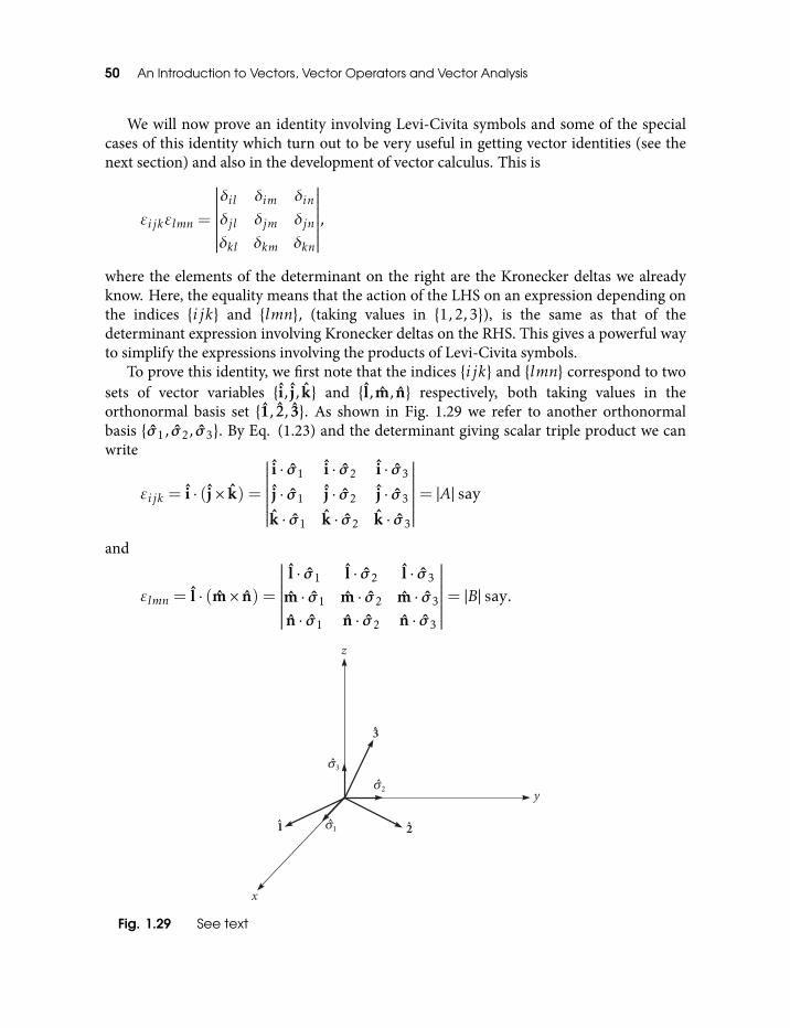
50 An Introduction to Vectors, Vector Operators and Vector Analysis
We will now prove an identity involving Levi-Civita symbols and some of the specialcases of this identity which turn out to be very useful in getting vector identities (see thenext section) and also in the development of vector calculus. This is
εijkεlmn =
∣∣∣∣∣∣∣∣∣δil δim δinδjl δjm δjnδkl δkm δkn
∣∣∣∣∣∣∣∣∣,where the elements of the determinant on the right are the Kronecker deltas we alreadyknow. Here, the equality means that the action of the LHS on an expression depending onthe indices ijk and lmn, (taking values in 1,2,3), is the same as that of thedeterminant expression involving Kronecker deltas on the RHS. This gives a powerful wayto simplify the expressions involving the products of Levi-Civita symbols.
To prove this identity, we first note that the indices ijk and lmn correspond to twosets of vector variables i, j, k and l,m, n respectively, both taking values in theorthonormal basis set 1, 2, 3. As shown in Fig. 1.29 we refer to another orthonormalbasis σ1, σ2, σ3. By Eq. (1.23) and the determinant giving scalar triple product we canwrite
εijk = i · (j× k) =
∣∣∣∣∣∣∣∣∣i · σ1 i · σ2 i · σ3
j · σ1 j · σ2 j · σ3
k · σ1 k · σ2 k · σ3
∣∣∣∣∣∣∣∣∣= |A| say
and
εlmn = l · (m× n) =
∣∣∣∣∣∣∣∣∣l · σ1 l · σ2 l · σ3
m · σ1 m · σ2 m · σ3
n · σ1 n · σ2 n · σ3
∣∣∣∣∣∣∣∣∣= |B| say.
Fig. 1.29 See text
Getting Concepts and Gathering Tools 51
Here, |A| and |B| are the determinants of the corresponding matrices. Using the factthat the determinant of a matrix is the same as that of its transpose and that the product ofthe determinants of two matrices is the determinant of their product, (see Appendix A),we get,
εijkεlmn = |A| · |B|= |A| · |BT |= |ABT |=
∣∣∣∣∣∣∣∣∣∣∣i · l i · m i · n
j · l j · m j · n
k · l k · m k · n
∣∣∣∣∣∣∣∣∣∣∣To understand the last equality, note that a typical element of ABT is (see Fig. 1.29)
(i · σ1)(l · σ1) + (i · σ2)(l · σ2) + (i · σ3)(l · σ3) = ix lx+ iy ly + iz lz = i · l.
Since the variables i, j, k and l,m, n take values in the orthonormal basis set 1, 2, 3,we have i · l = δil etc, giving us the desired identity.
Before proceeding further, we need to introduce a convention, called Einsteinsummation convention, regarding the sum over a term in an expression whose termsdepend on some index set, say i, j,k. As per this convention, a term in which an indexsay i is repeated is to be summed over that index. Thus, for example, εijkεilm =∑3i=1 εijkεilm, a sum in which at most one term survives. Also,
δkk =3∑k=1
δkk = δ11 + δ22 + δ33 = 3.
Henceforth, in this book, whenever applicable, Einstein summation convention will alwaysbe assumed to apply, unless stated otherwise. So you will have to be alert about this.
We can now obtain some special cases of the result we just proved. Thus, thedeterminant for εijkεilm can be obtained from that for εijkεlmn by replacing l by i. Sinceall the indices i, j,k must be different, (otherwise εijk = 0), we must have i · i = 1 andj · i = 0 = k · i. Substituting these values in the determinant and evaluating it we get
εijkεilm = δjlδkm − δjmδkl .
Next, consider
εijkεijl = δjjδkl − δkjδjl = 3δkl − δkl = 2δkl .
Here, we have used δjj = 3 and δkjδjl = δkl which we proved above (see Eq. (1.24)).Finally, we have,
εijkεijk = 2δkk = 2 · 3 = 6.
52 An Introduction to Vectors, Vector Operators and Vector Analysis
Let us try and express the vector product in terms of the Levi-Civita symbols. UsingEqs (1.7) and (1.13) we can express the ith component of a×b as
(a×b)i = i · (a×b) = ajbk − akbj = εijkajbk . (1.25)
In the last term, a sum over indices j = 1,2,3 and k = 1,2,3 is implied, which is a sum ofnine terms. However, seven out of these nine terms vanish, because the corresponding εijkvanish due to repeated indices, so that only two terms survive. Thus,
(a×b)1 = ε123a2b3 + ε132a3b2 = a2b3 − a3b2.
Check that other terms in the implied sum vanish.Subsequently, we will have many occasions to use these results.
1.12 Vector IdentitiesIn this section, we equip our toolbox by acquiring some of the most penetrating tools ofvector algebra and analysis. These are the so called vector identities. A vector identity isan equality involving vector variables which holds good for every possible (vector) valuethat these variables can take. From our school days, we are familiar with trigonometricidentities like sin2θ+cos2θ = 1 or cos(A+B) = cos(A)cos(B)−sin(A)sin(B) whichhold for all possible values of the angles involved. In this section, we deal with the identitiesinvolving the vector variables. We learn about the identities involving vector operators in alater section. All the vector identities can be proved using Levi-Civita notation.
We prove the vector identities one by one.We first prove
a× (b× c) = (a · c)b− (a ·b)c. (1.26)
We have,
[a× (b× c)]i = εijkaj(b× c)k
= εkijεklmajblcm
= (δilδjm − δimδjl)ajblcm
= (ajcj)bi − (ajbj)ci
= (a · c)bi − (a ·b)ci .
Thus, the ith components (i = 1,2,3) of both the sides are equal, which proves theidentity. This identity tells us that the vector product of a polar and an axial vector equals
Getting Concepts and Gathering Tools 53
the difference of two polar vectors and hence is itself a polar vector. By permuting a,b,cin cyclic order in the identity a× (b× c) = (a · c)b− (a ·b)c we get two more identities,
b× (c× a) = (a ·b)c− (b · c)a
c× (a×b) = (b · c)a− (c · a)b.
Adding these three identities we get
a× (b× c) + c× (a×b) +b× (c× a) = 0.
The next identity is
(a×b) · (c×d) = (a · c)(b ·d)− (a ·d)(b · c).
We have,
(a×b)i(c×d)i = εijkεilmajbkcldm
= (δjlδkm − δjmδkl)ajbkcldm
= (ajcj)(bkdk)− (ajdj)(bkck)
= (a · c)(b ·d)− (a ·d)(b · c).
Exercise Prove the identity
(a×b)× (c×d) = (a · c×d)b− (b · c×d)a
= (a ·b×d)c− (a ·b× c)d.
Throughout the remaining text, all these identities will be used very frequently. Werecommend that you practice these identities by using them in as large variety of problemsas possible. For future convenience we list these identities once again, separately. In theremaining part of the book we will refer to these identities by their Roman serial numbersin this list.
(I) a× (b× c) = (a · c)b− (a ·b)c.
(II) (a×b) · (c×d) = (a · c)(b ·d)− (a ·d)(b · c).(III) a× (b× c) + c× (a×b) +b× (c× a) = 0.
(IV) (a×b)× (c×d) = (a · c×d)b− (b · c×d)a = (a ·b×d)c− (a ·b× c)d.
54 An Introduction to Vectors, Vector Operators and Vector Analysis
Exercise Show that
(a×b) · (c×d)× (e× f) = [abd][cef]− [abc][def],
= [abc][fcd]− [abf][ecd],
= [cda][bef]− [cdb][aef],
where we have used Grassmann notation for the scalar triple product.
1.13 Vector EquationsAn equation involving expressions of vectors and scalars is a (algebraic) vector equation.A vector equation can be solved either for an unknown vector or for an unknown scalarin it. The novel aspect of vector equations is that they can be transformed and solvedusing vector algebra. Here, we give some simple results regarding vector equations. We willhave occasions to solve vector equations especially in the next chapter. In this section weuse x,y,z, . . . for vector variables (unknowns) and a,b,c, . . . for known or constant vectorsappearing in an equation. As usual, greek letters are used for scalars.
(i) A linear equation in one unknown vector may be solved similar to such a scalarequation. Thus, the equation
λx+ µa = αx+ βb
can be solved by shifting terms on either side of the equation giving
x =( β
λ−α
)b−
( µ
λ−α
)a.
(ii) The vector equation λx + µa = νb where λ , 0,µ,ν are given constant scalars anda,b are constant vectors has a unique solution x = 1
λ(νb−µa).The fact that this equation admits a solution can be trivially checked. We have to
subtract µa on both sides and then divide by λ on both sides to get the given solution.Properties of vector addition and scalar multiplication allow these operations. Nextwe can substitute the given solution for x in the equation and check that it satisfiesthe equation. Thus the given solution is a solution of the given equation. To see thatthis solution is unique, assume two solutions x1 and x2, substitute in the equationand equate the two resulting expressions to show that x1 = x2.
(iii) λa+µb = c to be solved for two unknown scalars λ,µwhere all the three vectors aregiven constant non-zero vectors.
Taking cross product by b on both sides of the equation from right we get
λa×b = c×b.
Getting Concepts and Gathering Tools 55
Dotting both sides with c×b we get
λ=|c×b|2
(a×b) · (c×b),
assuming that the pairs a,b and also b,c are not parallel to each other. If a and b areparallel, we have a = νb and the equation reduces to (λν+µ)b = c. This shows thatb and c are also parallel, hence there are infinite number of solutions of λ and µ. Toget µ, we take cross product by a on both sides of the equation and proceed exactly asbefore. The result is
µ=|c× a|2
(b× a) · (c× a).
(iv) The equation x · a = λ where λ is a known scalar and a is a known non-zero vector.We rewrite the equation as
x · a = λa−1 · a, or (x−λa−1) · a = 0,
which implies that the vector x−λa−1 is orthogonal to a so that
x−λa−1 = a×b,
where b is a non-zero arbitrary vector, not parallel to a. Thus,
x = λa−1 + a×b
is the general solution we are seeking.(v) The equation x×a = b where a , 0 and b are known vectors admits a solution if and
only if a ·b = 0.To prove the necessity, assume that the equation admits a solution x. Hence,
a · b = a · (x × a) = 0, which establishes the necessity. Now assume a · b = 0and substitute the expansion of a vector x in terms of three non-coplanar vectors
x = λa+ µb+ ν(a×b)
(with λ,µ,ν scalars), in the equation. We get, after some algebra and using a ·b = 0,
µ(b× a) + [ν(a · a)− 1]b = 0.
Since the vectors b × a and b are linearly independent, both the coefficients mustvanish separately, giving
µ= 0 and ν|a|2 − 1 = 0
56 An Introduction to Vectors, Vector Operators and Vector Analysis
which means ν = 1|a|2 and leads to
x = λa+1|a|2
(a×b) = λa+ (a−1 ×b),
which satisfies the given equation irrespective of the value of the scalar λ.
(vi) The equations x · a = λ and x× b = c where a,b,c are given vectors with a,b non-orthogonal (a ·b , 0,) uniquely determine vector x.
Crossing the second equation on the left by a we get
a× (x×b) = a× c,
or, using identity I,
(a ·b)x− (a · x)b = a× c
or,
x =1
a ·b(λb+ a× c)
which satisfies both the equations.To get the uniqueness, suppose that two vectors x1 , x2 satisfy the given equations.
This leads to
(x1 − x2) · a = 0 and (x1 − x2)×b = 0.
Therefore, the vector a is perpendicular to and vector b is parallel to the vector x1−x2.This makes vectors a and b mutually orthogonal, contradicting the assumption thatthey are not. Thus, we must require
x1 − x2 = 0 or, x1 = x2.
Exercise Show that αa−1 is a solution of
a · y = α, (α , 0).
Show that there are infinitely many solutions.
Exercise show that the necessary and sufficient condition for the equation
a× y = b
where a and b are known and a , 0, posseses a solution is a ·b = 0.
Getting Concepts and Gathering Tools 57
Solution Since
a ·b = a · (a× y) = 0,
the condition is necessary.Now suppose a ·b = 0. Then,
a× (b× a−1) = b− (a ·b)a−1 = b.
Thus,
y = b× a−1
satisfies a× y = b. The solution is not unique since
y = b× a−1 +λa
is also a solution.
Exercise Show that a vector is uniquely determined if its dot product with three non-coplanar vectors are known.
Hint Expand the vector in the basis comprising the given three non-coplanar vectors.
Exercise The resultant of two vectors is equal in magnitude to one of them and isperpendicular to it. Find the other vector.
Hint Let a+b = c with |a|= |c|= λ say and let |b|= µ. Also, a · c = 0. (Draw a figure).Take the unit vectors along a and c as the orthonormal basis. Express a,b and c in terms ofthis basis and use the first equation. Find b in terms of the angle θ it makes with c and itsmagnitude λ.
Answer θ = π4 , µ=
√2λ. You can get this answer just by drawing the figure.
1.14 Coordinate Systems Revisited: Curvilinear CoordinatesAs we go along any one of the coordinate axes, say x axis, only the correspondingcoordinate changes while the other two remain unchanged. Let us define a coordinate lineto be that curve in R3 along which only one of the coordinates changes, while other tworemain the same. Now these coordinate lines need not be straight lines! The coordinatesystems for which one or more coordinate lines are curves other than straight lines arecalled curvilinear coordinate systems. In fact we can set up coordinate systems in whichthe coordinate lines are circles!
1.14.1 Spherical polar coordinates
One such very useful coordinate system is the so called spherical polar coordinate systemwhich we now set up (see Fig. 1.30). First, we fix a right handed rectangular Cartesiancoordinate system at the origin O. Mark out a point P in space and draw the line joining
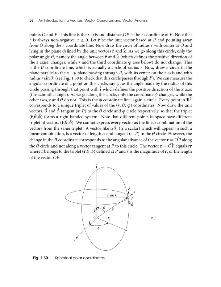
58 An Introduction to Vectors, Vector Operators and Vector Analysis
points O and P . This line is the r axis and distance OP is the r coordinate of P . Note thatr is always non-negative, r ≥ 0. Let r be the unit vector based at P and pointing awayfrom O along the r coordinate line. Now draw the circle of radius r with center at O andlying in the plane defined by the unit vectors r and k. As we go along this circle, only thepolar angle θ, namely the angle between r and k (which defines the positive direction ofthe z axis), changes, while r and the third coordinate φ (see below) do not change. Thisis the θ coordinate line, which is actually a circle of radius r . Now, draw a circle in theplane parallel to the x − y plane passing through P , with its center on the z axis and withradius r sinθ. (see Fig. 1.30 to check that this circle passes through P ). We can measure theangular coordinate of a point on this circle, say φ, as the angle made by the radius of thiscircle passing through that point with i which defines the positive direction of the x axis(the azimuthal angle). As we go along this circle, only the coordinate φ changes, while theother two, r and θ do not. This is the φ coordinate line, again a circle. Every point in R3
corresponds to a unique triplet of values of the (r , θ, φ) coordinates. Now draw the unitvectors, θ and φ tangent (at P ) to the θ circle and φ circle respectively, so that the triplet(r,θ,φ) forms a right handed system. Note that different points in space have differenttriplet of vectors (r,θ,φ). We cannot express every vector as the linear combination of thevectors from the same triplet. A vector like αθ, (α a scalar) which will appear in such alinear combination, is a vector of length α and tangent (at P ) to the θ circle. However, thechange in the θ coordinate corresponds to the angular advance of the vector r = ~OP alongthe θ circle and not along a vector tangent at P to this circle. The vector r = ~OP equals r rwhere r belongs to the triplet (r,θ,φ) defined at P and r is the magnitude of r, or the lengthof the vector ~OP .
Fig. 1.30 Spherical polar coordinates
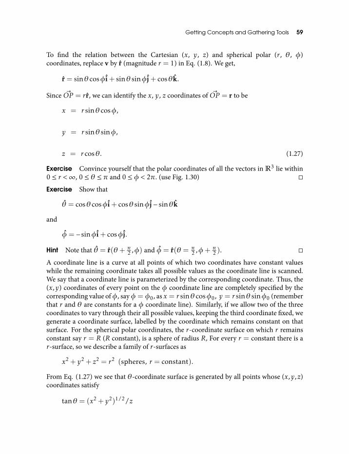
Getting Concepts and Gathering Tools 59
To find the relation between the Cartesian (x, y, z) and spherical polar (r, θ, φ)coordinates, replace v by r (magnitude r = 1) in Eq. (1.8). We get,
r = sinθ cosφi+ sinθ sinφj+ cosθk.
Since ~OP = r r, we can identify the x, y, z coordinates of ~OP = r to be
x = r sinθ cosφ,
y = r sinθ sinφ,
z = r cosθ. (1.27)
Exercise Convince yourself that the polar coordinates of all the vectors in R3 lie within0 ≤ r <∞, 0 ≤ θ ≤ π and 0 ≤ φ < 2π. (use Fig. 1.30)
Exercise Show that
θ = cosθ cosφi+ cosθ sinφj− sinθk
and
φ = −sinφi+ cosφj.
Hint Note that θ = r(θ+ π2 ,φ) and φ = r(θ = π
2 ,φ+ π2 ).
A coordinate line is a curve at all points of which two coordinates have constant valueswhile the remaining coordinate takes all possible values as the coordinate line is scanned.We say that a coordinate line is parameterized by the corresponding coordinate. Thus, the(x,y) coordinates of every point on the φ coordinate line are completely specified by thecorresponding value ofφ, sayφ = φ0, as x = r sinθ cosφ0, y = r sinθ sinφ0 (rememberthat r and θ are constants for a φ coordinate line). Similarly, if we allow two of the threecoordinates to vary through their all possible values, keeping the third coordinate fixed, wegenerate a coordinate surface, labelled by the coordinate which remains constant on thatsurface. For the spherical polar coordinates, the r-coordinate surface on which r remainsconstant say r = R (R constant), is a sphere of radius R, For every r = constant there is ar-surface, so we describe a family of r-surfaces as
x2 + y2 + z2 = r2 (spheres, r = constant).
From Eq. (1.27) we see that θ-coordinate surface is generated by all points whose (x,y,z)coordinates satisfy
tanθ = (x2 + y2)1/2/z
60 An Introduction to Vectors, Vector Operators and Vector Analysis
which are circular cones θ = constant. The φ coordinate surfaces are generated by allpoints whose (x,y,z) coordinates satisfy
tanφ = y/x
and z is arbitrary. These are half planes, that is, the planes which terminate at the z axis,because the other half plane, on the other side of the z axis corresponds to π+φ. All thesecoordinate surfaces are depicted in Fig. 1.31.
Given any point in space, with coordinates R,θ0,φ0, the coordinate surfaces r = R,θ = θ0 and φ = φ0 pass through that point. The φ coordinate line is the intersection ofthe r = R, θ = θ0 surfaces and lies in a plane parallel to xy plane while θ coordinate lineis the intersection of r = R and φ = φ0 surfaces and lies in a plane normal to xy plane.Therefore, the vectors θ,φ tangent to these curves must be mutually perpendicular. Theplane containing these two vectors is tangent to the sphere r = R at the given point, so thatthe unit vector r must be normal to both θ,φ. Thus, the vectors r,θ,φ form an orthonormalbasis. Such a system is called an orthogonal curvilinear coordinate system.
Fig. 1.31 Coordinate surfaces are x2+y2+z2 = r2 (spheres r = constant) tanθ =(x2 + y2)1/2/z (circular cones, θ = constant) tanφ = y/x (half planesφ = constant)
1.14.2 Parabolic coordinates
We shall learn about one more orthogonal curvilinear coordinate system, namely, theparabolic coordinate system. We first set up a right handed Cartesian coordinate systemwith orthonormal basis (i, j, k). A point in space having Cartesian coordinates (x,y,z)
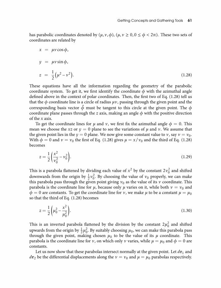
Getting Concepts and Gathering Tools 61
has parabolic coordinates denoted by (µ,ν,φ), (µ,ν ≥ 0,0 ≤ φ < 2π). These two sets ofcoordinates are related by
x = µν cosφ,
y = µν sinφ,
z =12
(µ2 − ν2
). (1.28)
These equations have all the information regarding the geometry of the paraboliccoordinate system. To get it, we first identify the coordinate φ with the azimuthal angledefined above in the context of polar coordinates. Then, the first two of Eq. (1.28) tell usthat the φ coordinate line is a circle of radius µν, passing through the given point and thecorresponding basis vector φ must be tangent to this circle at the given point. The φcoordinate plane passes through the z axis, making an angle φ with the positive directionof the x axis.
To get the coordinate lines for µ and ν, we first fix the azimuthal angle φ = 0. Thismean we choose the xz or y = 0 plane to see the variations of µ and ν. We assume thatthe given point lies in the y = 0 plane. We now give some constant value to ν, say ν = ν0.With φ = 0 and ν = ν0 the first of Eq. (1.28) gives µ = x/ν0 and the third of Eq. (1.28)becomes
z =12
(x2
ν20
− ν20
). (1.29)
This is a parabola flattened by dividing each value of x2 by the constant 2ν20 and shifted
downwards from the origin by 12ν
20 . By choosing the value of ν0 properly, we can make
this parabola pass through the given point giving ν0 as the value of its ν coordinate. Thisparabola is the coordinate line for µ, because only µ varies on it, while both ν = ν0 andφ = 0 are constants. To get the coordinate line for ν, we make µ to be a constant µ = µ0so that the third of Eq. (1.28) becomes
z =12
(µ2
0 −x2
µ20
). (1.30)
This is an inverted parabola flattened by the division by the constant 2µ20 and shifted
upwards from the origin by 12µ
20. By suitably choosing µ0, we can make this parabola pass
through the given point, making chosen µ0 to be the value of its µ coordinate. Thisparabola is the coordinate line for ν, on which only ν varies, while µ = µ0 and φ = 0 areconstants.
Let us now show that these parabolas intersect normally at the given point. Let dr1 anddr2 be the differential displacements along the ν = ν0 and µ = µ0 parabolas respectively.
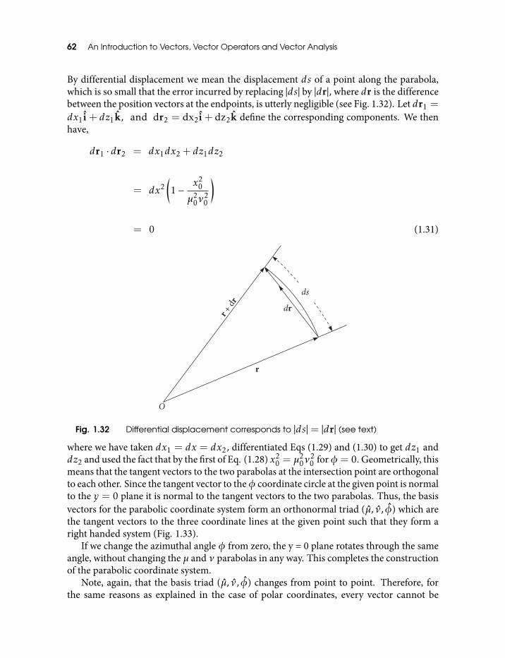
62 An Introduction to Vectors, Vector Operators and Vector Analysis
By differential displacement we mean the displacement ds of a point along the parabola,which is so small that the error incurred by replacing |ds| by |dr|, where dr is the differencebetween the position vectors at the endpoints, is utterly negligible (see Fig. 1.32). Let dr1 =dx1i + dz1k, and dr2 = dx2i + dz2k define the corresponding components. We thenhave,
dr1 · dr2 = dx1dx2 + dz1dz2
= dx2(1−
x20
µ20ν
20
)
= 0 (1.31)
Fig. 1.32 Differential displacement corresponds to |ds|= |dr| (see text)
where we have taken dx1 = dx = dx2, differentiated Eqs (1.29) and (1.30) to get dz1 anddz2 and used the fact that by the first of Eq. (1.28) x2
0 = µ20ν
20 forφ = 0. Geometrically, this
means that the tangent vectors to the two parabolas at the intersection point are orthogonalto each other. Since the tangent vector to theφ coordinate circle at the given point is normalto the y = 0 plane it is normal to the tangent vectors to the two parabolas. Thus, the basisvectors for the parabolic coordinate system form an orthonormal triad (µ, ν, φ) which arethe tangent vectors to the three coordinate lines at the given point such that they form aright handed system (Fig. 1.33).
If we change the azimuthal angle φ from zero, the y = 0 plane rotates through the sameangle, without changing the µ and ν parabolas in any way. This completes the constructionof the parabolic coordinate system.
Note, again, that the basis triad (µ, ν, φ) changes from point to point. Therefore, forthe same reasons as explained in the case of polar coordinates, every vector cannot be
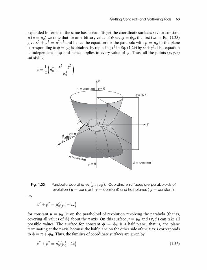
Getting Concepts and Gathering Tools 63
expanded in terms of the same basis triad. To get the coordinate surfaces say for constantµ (µ = µ0) we note that for an arbitrary value of φ say φ = φ0, the first two of Eq. (1.28)give x2 + y2 = µ2ν2 and hence the equation for the parabola with µ = µ0 in the planecorresponding toφ = φ0 is obtained by replacing x2 in Eq. (1.29) by x2+y2. This equationis independent of φ and hence applies to every value of φ. Thus, all the points (x,y,z)satisfying
z =12
(µ2
0 −x2 + y2
µ20
)
Fig. 1.33 Parabolic coordinates (µ,ν,φ). Coordinate surfaces are paraboloids ofrevolution (µ= constant, ν = constant) and half-planes (φ = constant)
or,
x2 + y2 = µ20
(µ2
0 − 2z)
for constant µ = µ0 lie on the paraboloid of revolution revolving the parabola (that is,covering all values of φ) about the z axis. On this surface µ = µ0 and (ν,φ) can take allpossible values. The surface for constant φ = φ0 is a half plane, that is, the planeterminating at the z axis, because the half plane on the other side of the z axis correspondsto φ = π+φ0. Thus, the families of coordinate surfaces are given by
x2 + y2 = µ20
(µ2
0 − 2z)
(1.32)
64 An Introduction to Vectors, Vector Operators and Vector Analysis
(paraboloids of revolution, µ= constant),
x2 + y2 = µ20
(µ2
0 + 2z)
(1.33)
(paraboloids of revolution, ν = constant),
tanφ = y/x (1.34)
(half planes φ = constant).
Exercise Justify the coordinate lines and coordinate surfaces, shown in Fig. 1.34, for thecylindrical coordinates (0 ≤ ρ <∞, 0 ≤ φ < 2π, −∞ < z <+∞) defined by
x = ρcosφ,
y = ρ sinφ,
z = z, (1.35)
Fig. 1.34 Cylindrical coordinates (ρ,φ,z). Coordinate surfaces are circular cylinders(ρ = constant), half-planes (φ = constant) intersecting on the z-axis, andparallel planes (z = constant)
where the coordinate surfaces are given by
x2 + y2 = ρ2
(circular cylinders, ρ = constant),
tanφ = y/x
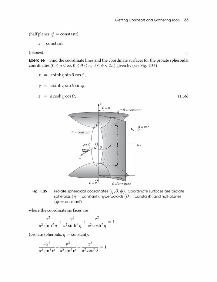
Getting Concepts and Gathering Tools 65
(half planes, φ = constant),
z = constant
(planes).
Exercise Find the coordinate lines and the coordinate surfaces for the prolate spheroidalcoordinates (0 ≤ η <∞, 0 ≤ θ ≤ π, 0 ≤ φ < 2π) given by (see Fig. 1.35)
x = asinhη sinθ cosφ,
y = asinhη sinθ sinφ,
z = acoshη cosθ, (1.36)
Fig. 1.35 Prolate spheroidal coordinates (η,θ,φ). Coordinate surfaces are prolatespheroids (η = constant), hyperboloids (θ = constant), and half-planes(φ = constant)
where the coordinate surfaces are
x2
a2 sinh2η+
y2
a2 sinh2η+
z2
a2 cosh2η= 1
(prolate spheroids, η = constant),
−x2
a2 sin2θ−
y2
a2 sin2θ+
z2
a2 cos2θ= 1
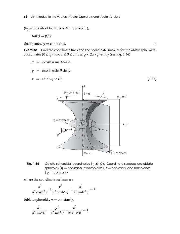
66 An Introduction to Vectors, Vector Operators and Vector Analysis
(hyperboloids of two sheets, θ = constant),
tanφ = y/x
(half planes, φ = constant).
Exercise Find the coordinate lines and the coordinate surfaces for the oblate spheroidalcoordinates (0 ≤ η <∞, 0 ≤ θ ≤ π, 0 ≤ φ < 2π) given by (see Fig. 1.36)
x = acoshη sinθ cosφ,
y = acoshη sinθ sinφ,
z = asinhη cosθ, (1.37)
Fig. 1.36 Oblate spheroidal coordinates (η,θ,φ). Coordinate surfaces are oblatespheroids (η = constant), hyperboloids (θ = constant), and half-planes(φ = constant)
where the coordinate surfaces are
x2
a2 cosh2η+
y2
a2 cosh2η+
z2
a2 sinh2η= 1
(oblate spheroids, η = constant),
x2
a2 sin2θ+
y2
a2 sin2θ− z2
a2 cos2θ= 1
Getting Concepts and Gathering Tools 67
(hyperboloids of one sheet, θ = constant),
tanφ = y/x
(half planes, φ = constant).
1.15 Vector FieldsWe want to understand the concept of a vector field. The best way for us is to understandit operatively first, which will then lead to its mathematical meaning. To get to the physicalmeaning of a field, we must apply the principle of relativity by Einstein, however, we willnot attempt that in this book. We first choose a point in space to be the origin O. Wethen obtain the position vector of a point P in space based at the origin O. Thereafter,we base a vector giving the value of some physical quantity at P . We now imagine thatwe base some vector giving a value of this physical quantity at every point in space, or insome region of space. This association, of the set of vectors giving values of a physicalquantity with the set of position vectors or points in space (including the origin) is called avector field. To give this procedure a meaning, we must seek the rule by which the vectorvalues of a vector quantity are associated with the points in space. This rule can be eithera one to one or many to one correspondence between the points in space and the vectorvalues of a vector quantity (that is, the vectors assigned to different points in space couldbe different or equal). In other words, this rule is a function taking in a position vectorand returning the vector value of a vector quantity corresponding to that position vectoror the point. Thus, the vector field is the vector valued function of the position vectors.A function taking in a position vector specifying a point in space and returning a scalaris said to generate a scalar field. A function generating a vector field or a scalar field canbe viewed as the function of the coordinates, that is, a function which takes in a triplet ofreal numbers (components of the position vector or coordinates specifying a point in space)and returns another triplet of real numbers (components of the vector to be assigned to thatpoint) or a scalar. When viewed as a function of coordinates, a function generating a field isrequired to be a ‘point function’ that is, the value of the function at any point must remaininvariant even if we switch over to another coordinate system changing the coordinatesof that point. A coordinate transformation will yield a new function of new coordinates,which, when evaluated at the new coordinates of the same point, must give the same valueof the field at that point. A field value at a point cannot depend on which coordinate systemwe use to refer to that point. Suppose a function of the latitude and longitude returns thetemperature at a place on earth with the given latitude and longitude. If we specify thecoordinates of the points on earth using a rotated mesh of latitude-longitude and use thecorresponding transformation to get a new function of new coordinates for this scalar field,then this new function, when evaluated at the new coordinates of the same place, must givethe same temperature. Temperature at a place cannot depend on which coordinate systemwe choose to refer to that place.
Physically, a vector field is produced by its sources and the problem is to relate this fieldto the characteristic properties of its sources. These relations are often expressed as
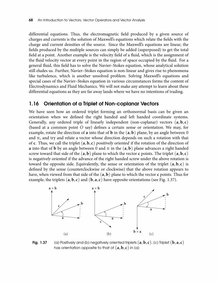
68 An Introduction to Vectors, Vector Operators and Vector Analysis
differential equations. Thus, the electromagnetic field produced by a given source ofcharges and currents is the solution of Maxwell’s equations which relate the fields with thecharge and current densities of the source. Since the Maxwell’s equations are linear, thefields produced by the multiple sources can simply be added (superposed) to get the totalfield at a point. Another example is the velocity field of a fluid, which is the assignment ofthe fluid velocity vector at every point in the region of space occupied by the fluid. For ageneral fluid, this field has to solve the Navier–Stokes equation, whose analytical solutionstill eludes us. Further, Navier–Stokes equation is non-linear and gives rise to phenomenalike turbulence, which is another unsolved problem. Solving Maxwell’s equations andspecial cases of the Navier–Stokes equation in various circumstances forms the content ofElectrodynamics and Fluid Mechanics. We will not make any attempt to learn about thesedifferential equations as they are far away lands where we have no intentions of trading.
1.16 Orientation of a Triplet of Non-coplanar VectorsWe have seen how an ordered triplet forming an orthonormal basis can be given anorientation when we defined the right handed and left handed coordinate systems.Generally, any ordered triple of linearly independent (non-coplanar) vectors (a,b,c)(based at a common point O say) defines a certain sense or orientation. We may, forexample, rotate the direction of a into that of b in the (a,b) plane, by an angle between 0and π, and try and relate a vector whose direction depends on such a rotation with thatof c. Thus, we call the triplet (a,b,c) positively oriented if the rotation of the direction ofa into that of b by an angle between 0 and π in the (a,b) plane advances a right handedscrew toward that side of the (a,b) plane to which the vector c points. The triplet (a,b,c)is negatively oriented if the advance of the right handed screw under the above rotation istoward the opposite side. Equivalently, the sense or orientation of the triplet (a,b,c) isdefined by the sense (counterclockwise or clockwise) that the above rotation appears tohave, when viewed from that side of the (a,b) plane to which the vector c points. Thus forexample, the triplets (a,b,c) and (b,a,c) have opposite orientations (see Fig. 1.37).
Fig. 1.37 (a) Positively and (b) negatively oriented triplets (a,b,c), (c) Triplet (b,a,c)has orientation opposite to that of (a,b,c) in (a)
Getting Concepts and Gathering Tools 69
We shall now show that the necessary and sufficient condition for a triplet (a,b,c) tobe positively oriented is that c · (a×b) or any of its cyclic permutations exceeds zero.
Suppose (a,b,c) are positively oriented. Then from the definitions of the positiveorientation and the vector product we see that both (a × b) and c are on the same side ofthe (a,b) plane. This implies that the angle between (a×b) and c is less than π/2 whichmeans c · (a×b) > 0.
Suppose c · (a × b) > 0. This means the angle between (a × b) and c is less than π/2,or, (a× b) and c are on the same side of the (a,b) plane, or the rotation from a toward badvances a right handed screw on the same side of the (a,b) plane to which c points. Inother words, (a,b,c) are positively oriented.
Since the scalar triple product is invariant under cyclic permutations of factors, aboveproof applies to all cyclic permutations of c · (a × b). Thus, we can conclude that theorientation of (a,b,c) is invariant under the cyclic permutation of (a,b,c).
Triplets (a,b,c) and (d,e,f) are oriented (mutually) positively (negatively) withrespect to each other if they have the same (opposite) orientations. In particular, (a,b,c)is oriented positively (negatively) with respect to an orthonormal basis (e1, e2, e3) orthe corresponding coordinate axes (x,y,z) if (a,b,c) and (e1, e2, e3) have the same(opposite) orientations. Whether a given triplet (a,b,c) is oriented positively ornegatively with respect to an orthonormal basis (e1, e2, e3) is decided, respectively, by thepositive or negative sign of
det(a,b,c) =
∣∣∣∣∣∣∣∣∣a1 a2 a3
b1 b2 b3
c1 c2 c3
∣∣∣∣∣∣∣∣∣ , (1.38)
where each row consists of the components of the corresponding vector with respect tothe orthonormal basis (e1, e2, e3) (see the second exercise on page 39). Exchanging thefirst two columns of this determinant amounts to exchanging x,y axes or changing over toa coordinate system with different handedness. This changes the sign of the determinant,so that orientation of (a,b,c) with respect to the new coordinate system becomesopposite to that with respect to the previous one. Thus, the sign of the determinantcomprising the components of a given triplet of vectors (a,b,c) decides the orientation of(a,b,c) with respect to the corresponding orthonormal basis (e1, e2, e3), or, assometimes said, with respect to the (x,y,z) coordinates or axes. Thus, the sign of thedeterminant in Eq. (1.38) does not have a geometrical meaning independent of acoordinate system. However, a statement like ‘two non-coplanar ordered triplets have thesame or the opposite orientation’ has a coordinate free geometrical meaning.
Consider two ordered triplets of non-coplanar vectors a1,a2,a3 and b1,b2,b3. The twosets have the same orientation, that is, are both positively or both negatively oriented withrespect to a common coordinate system (x1,x2,x3) if and only if the condition
det(a1,a2,a3) ·det(b1,b2,b3) > 0
70 An Introduction to Vectors, Vector Operators and Vector Analysis
is satisfied. Using identity (A.31), we can write this condition in the form
[a1,a2,a3;b1,b2,b3] > 0 (1.39)
where the symbol on the left denotes a function of six vector variables defined by
[a1,a2,a3;b1,b2,b3] =
∣∣∣∣∣∣∣∣∣a1 ·b1 a1 ·b2 a1 ·b3
a2 ·b1 a2 ·b2 a2 ·b3
a3 ·b1 a3 ·b2 a3 ·b3
∣∣∣∣∣∣∣∣∣ · (1.40)
Note that for b1 = a1,b2 = a2,b3 = a3 Eq. (1.40) reduces to the definition of theGram determinant Γ (a1,a2,a3) (see Appendix A). Equations (1.39) and (1.40) show that,for two ordered triplets having the same orientation (relative to a coordinate system) is ageometric property independent of any particular Cartesian coordinate system used. Wedenote this property symbolically by
Ω(a1,a2,a3) =Ω(b1,b2,b3) (1.41)
and the property of having opposite orientation by
Ω(a1,a2,a3) = −Ω(b1,b2,b3). (1.42)
We can combine these two equations in a single one:
Ω(a1,a2,a3) = sgn[a1,a2,a3;b1,b2,b3]Ω(b1,b2,b3). (1.43)
The last three equations are meaningful even if we do not assign a numeric value to theindividual orientation Ω. Equation (1.43) associates a value ±1 to the ratio of twoorientations, while Eqs (1.41) and (1.42) express equality or inequality of orientations. It ispossible to specify two possible orientations of triplets of vectors completely by assigningnumerical values say Ω = ±1 to these orientations by arbitrarily choosing the standardvalue +1 for the orientation of the basis vectors (e1, e2, e3) defining the coordinatesystem. Such a situation arises in science and engineering in the context of everymeasurable quantity. For example, equality of distances between points in space or eventhe ratio of distances have meaning even if no numerical values are assigned to theindividual distances. It is of course possible to assign numerical values to individualdistances such that the ratio of distances equals the ratio of the corresponding realnumbers. This requires an arbitrary selection of a “standard distance” or a unit of distanceto which all other distances are referred. Thus Eq. (1.41) is analogus to saying thatdistances between two pairs of points are equal without giving them specific values.
The triplet a1,a2,a3 is oriented positively or negatively with respect to (x1,x2,x3)coordinates according to whether they are oriented positively or negatively with respect tothe corresponding orthonormal basis (e1, e2, e3), that is, whether
Ω(a1,a2,a3) =Ω(e1, e2, e3) (1.44)
Getting Concepts and Gathering Tools 71
or
Ω(a1,a2,a3) = −Ω(e1, e2, e3). (1.45)
Sometimes, we denote the orientation of the coordinate system Ω(e1, e2, e3) byΩ(x1,x2,x3). Since the value of the determinant in Eq. (1.38) gives the signed volume ofthe parallelepiped spanned by a triplet of linearly independent vectors, for two suchtriplets of vectors we have,
[a1,a2,a3;b1,b2,b3] = ε1ε2V1V2 (1.46)
where V1 and V2 are, respectively the volumes of the parallelepipeds spanned by the twotriplets and the factors ε1,ε2 depend on their orientations with respect to the basis(e1, e2, e3) defining the coordinate system:
ε1 = sgn[a1,a2,a3; e1, e2, e3]
ε2 = sgn[b1,b2,b3; e1, e2, e3] (1.47)
and the relative orientation of the two triplets
ε1ε2 = sgn[a1,a2,a3;b1,b2,b3] (1.48)
is independent of the choice of the coordinate system and has the value +1 if theparallelepipeds have the same orientation but −1 if they have the opposite orientations. Ifthe two triplets refer to two different coordinate systems with the orthonormal bases(e1, e2, e3) and (h1, h2, h3) then,
ε1 = sgn[a1,a2,a3; e1, e2, e3]
ε2 = sgn[b1,b2,b3; h1, h2, h3]
µ = sgn[e1,e2,e3; h1, h2, h3] (1.49)
and the relative orientation of the two triplets, independent of the coordinate systems isgiven by
ε1ε2µ= sgn[a1,a2,a3;b1,b2,b3] (1.50)
and
[a1,a2,a3;b1,b2,b3] = ε1ε2µV1V2 (1.51)
where ε1,ε2,µ equal ±1 according to whether the corresponding triplets are orientedpositively or negatively. These equations are useful while dealing with triplets of vectors(generally based in different regions of space) which refer to different coordinate systems.
72 An Introduction to Vectors, Vector Operators and Vector Analysis
However, if it is possible to choose the two coordinate systems which are positivelyoriented with respect to each other, so as to ensure µ= +1, then Eq. (1.48) applies, whichdecides the relative orientation of the two triplets.
Our method of deciding the orientation of ordered sets of vectors by the sign of theirdeterminants can be applied to the doublets of non-collinear vectors spanning a plane. Wejust have to find out
[a1,a2;b1,b2] =
∣∣∣∣∣∣a1 ·b1 a1 ·b2
a2 ·b1 a2 ·b2
∣∣∣∣∣∣ · (1.52)
so that the equation
Ω(a1,a2) = sgn[a1,a2;b1,b2]Ω(b1,b2) (1.53)
decides whether the two doublets (a1,a2) and (b1,b2) have the same or oppositeorientations.
Exercise Let e1, e2 be an orthonormal basis in a plane. Show that the doublets e1, e2 ande2, e1 have opposite orientations.
Solution We have
[e1, e2; e2, e1] =
∣∣∣∣∣∣e1 · e2 e1 · e1
e2 · e2 e2 · e1
∣∣∣∣∣∣= −1, (1.54)
so that,
Ω(e2, e1) = −Ω(e1, e2).
1.16.1 Orientation of a plane
To orient a plane π we set up a 2-D coordinate system given by a pair of orthonormalvectors e1, e2 and define the orientation of the oriented plane π∗ by
Ω(π∗) =Ω(e1, e2). (1.55)
Any two linearly independent vectors (a1,a2) in the plane are oriented positively if
Ω(a1,a2) =Ω(π∗) =Ω(e1, e2).
Thus, all doublets positively oriented with respect to the basis (e1, e2) are positivelyoriented with respect to π∗.
An oriented plane π∗ can be characterized by a distinguished positive sense of rotation.If a pair of vectors a,b is oriented positively with respect toπ∗, the positive sense of rotationof π∗ is the sense of rotation by an angle less than π radians that takes the direction of ainto that of b.
Getting Concepts and Gathering Tools 73
Just as we can orient a plane, we can orient a 3-D region σ by specifying an orthonormalbasis (h1, h2, h3) and defining the orientation of the oriented region σ ∗ by
Ω(σ ∗) =Ω(h1, h2, h3).
All triplets which are positively oriented with respect to this basis are positively orientedwith respect to σ ∗. When an oriented plane π∗ lies in an oriented 3-D region σ ∗, we candefine the positive and negative sides of π∗. We take two independent vectors b and c in π∗that are positively oriented:
Ω(b,c) =Ω(π∗).
A third vector a, independent of b,c is said to point to the positive side of π∗ if
Ω(a,b,c) =Ω(σ ∗).
Since σ ∗ is oriented positively with respect to a Cartesian coordinate system, we can replacethis condition by
det(a,b,c) > 0.
If σ ∗ is oriented positively with respect to a right handed coordinate system, then thepositive side of an oriented plane π∗ is the one from which the positive sense of rotation inπ∗ appears counterclockwise.
2
Vectors and Analytic Geometry
Analytic geometry is the representation of curves and surfaces by algebraic equations. Ifthis representation is in R3, where each point in space and hence each position vector isrepresented by an ordered triplet of scalars, (that is, by coordinates), the correspondingequations representing geometrical objects involve coordinates of points on these objects.In such a case, analytic geometry is aptly called coordinate geometry. In this section, wetry and work with E3, in a coordinate free way to obtain equations for various geometricalcurves and surfaces. Since we axiomatize that both R3 and E3 are faithful representationsof real space in which objects move, the equations we derive are supposed to represent thepaths of moving particles or the surfaces confining their motions. In reality we do not dealwith point particles, therefore, the mathematical curves and surfaces described by theseequations are approximations to the actual motions.
2.1 Straight LinesGeometry, as we practice it today, is based on straight lines and planes as the basicelements to be used to build other forms of curves and surfaces. Therefore, we start byfinding out equations for the straight lines and planes. From the definition of the vectorproduct, given a fixed vector u , 0, all the points with position vectors x satisfying
x×u = 0 (2.1)
lie on the straight line on which u lies. Since x = 0 satisfies this equation, this line passesthrough the origin. Replacement of x by (x − a) in Eq. (2.1) for fixed vector a, rigidlydisplaces each point on the line given by Eq. (2.1) by the same vector a. The resulting lineis in the direction u and passing through the point a, given by the equation
(x− a)×u = 0. (2.2)
Each possible straight line in space is described by Eq. (2.2) for some a and u. We denotethe set of all points on the line byL , that is,L = x.
Vectors and Analytic Geometry 75
Exercise From Eq. (2.2) derive the following equations for the line L in terms ofrectangular coordinates in E3:
x1 − a1
u1=x2 − a2
u2=x3 − a3
u3,
where xk = x · σk ,ak = a · σk ,uk = u · σk , k = 1,2,3 and σ1, σ2, σ3 an orthonormal basis.
Hint [(x− a)×u] · σ3 = (x1 − a1)u2 − (x2 − a2)u1 etc.
Exercise(a) Show that Eq. (2.2) is equivalent to the parametric equation
x = a+λu.
(b) Describe the solution set x = x(t) of the parametric equation
x = a+ t2u
for all scalar values of the parameter t.
Hint(a) Equation (2.2) implies (x− a) · u ≡ λ.(b) x= half line with the direction u and endpoint a.
Dividing Eq. (2.2) by |u| and taking the constant term on the right, we get,
x× u = a× u.
We take the vector product on both sides from the left with u and use identity I to get
x = a− (u · a)u+ (u · x)u
= d+ (u · x)u, (2.3)
which we take to be the definition of the vector d. Noting that d · u = 0 we get, for thelength of vector x,
x2 = d2 + (u · x)2.
This distance is minimum for x = d or u · x = 0. This minimum distance is simply thedistance of the line from the origin and is given by d = |d| (see Fig. 2.1). We call d thedirectance [10](the directed distance) from the origin 0 to the line L . Its magnitude iscalled the distance from the origin to the line L . Note that d can be obtained from anypoint x on the line by subtracting the component of x along u from x (Eq. 2.3).
The vector
m = x× u
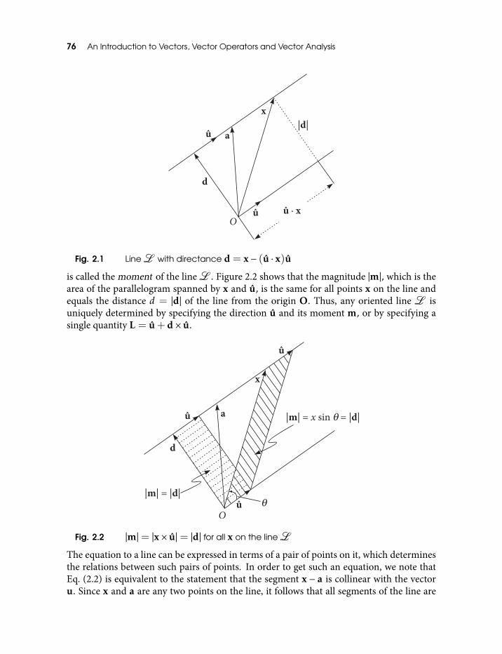
76 An Introduction to Vectors, Vector Operators and Vector Analysis
Fig. 2.1 LineL with directance d = x− (u · x)u
is called the moment of the lineL . Figure 2.2 shows that the magnitude |m|, which is thearea of the parallelogram spanned by x and u, is the same for all points x on the line andequals the distance d = |d| of the line from the origin O. Thus, any oriented line L isuniquely determined by specifying the direction u and its moment m, or by specifying asingle quantity L = u+d× u.
Fig. 2.2 |m|= |x× u|= |d| for all x on the lineL
The equation to a line can be expressed in terms of a pair of points on it, which determinesthe relations between such pairs of points. In order to get such an equation, we note thatEq. (2.2) is equivalent to the statement that the segment x − a is collinear with the vectoru. Since x and a are any two points on the line, it follows that all segments of the line are
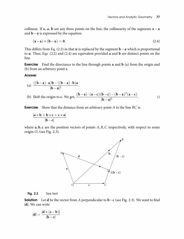
Vectors and Analytic Geometry 77
collinear. If x, a, b are any three points on the line, the collinearity of the segments x − aand b− a is expressed by the equation
(x− a)× (b− a) = 0. (2.4)
This differs from Eq. (2.2) in that u is replaced by the segment b− a which is proportionalto u. Thus, Eqs (2.2) and (2.4) are equivalent provided a and b are distinct points on theline.
Exercise Find the directance to the line through points a and b (a) from the origin and(b) from an arbitrary point c.
Answer
(a)((b− a) · a)b− ((b− a) ·b)a
|b− a|2.
(b) Shift the origin to c. We get,(b− a) · (a− c)(b− c)− (b− a)2(a− c)
|b− a|2.
Exercise Show that the distance from an arbitrary point A to the line BC is
|a×b+b× c+ c× a||b− c|
where a,b,c are the position vectors of points A,B,C respectively, with respect to someoriginO, (see Fig. 2.3).
Fig. 2.3 See text
Solution Let d be the vector fromA perpendicular to b−c (see Fig. 2.3). We want to find|d|. We can write
|d|=|d× (c−b)||b− c|
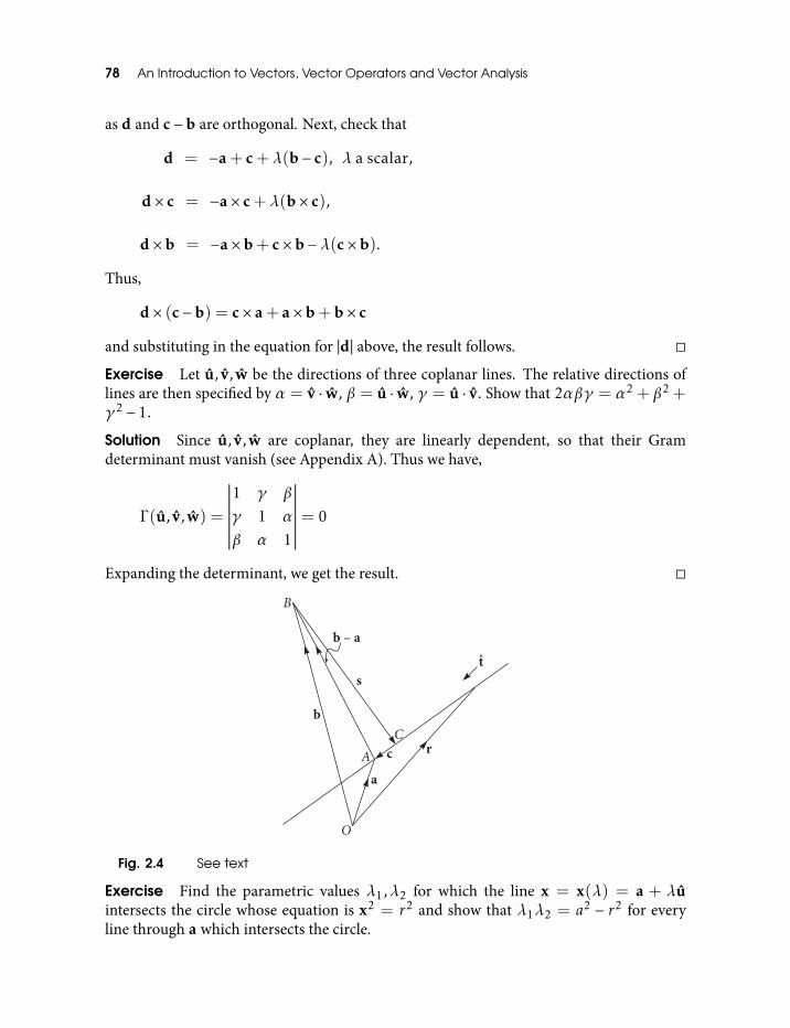
78 An Introduction to Vectors, Vector Operators and Vector Analysis
as d and c−b are orthogonal. Next, check that
d = −a+ c+λ(b− c), λ a scalar,
d× c = −a× c+λ(b× c),
d×b = −a×b+ c×b−λ(c×b).
Thus,
d× (c−b) = c× a+ a×b+b× c
and substituting in the equation for |d| above, the result follows.
Exercise Let u, v,w be the directions of three coplanar lines. The relative directions oflines are then specified by α = v · w, β = u · w, γ = u · v. Show that 2αβγ = α2 + β2 +γ2 − 1.
Solution Since u, v,w are coplanar, they are linearly dependent, so that their Gramdeterminant must vanish (see Appendix A). Thus we have,
Γ (u, v,w) =
∣∣∣∣∣∣∣∣∣1 γ β
γ 1 α
β α 1
∣∣∣∣∣∣∣∣∣= 0
Expanding the determinant, we get the result.
Fig. 2.4 See text
Exercise Find the parametric values λ1,λ2 for which the line x = x(λ) = a + λuintersects the circle whose equation is x2 = r2 and show that λ1λ2 = a2 − r2 for everyline through a which intersects the circle.
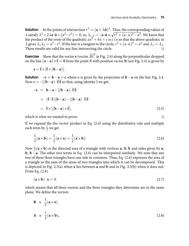
Vectors and Analytic Geometry 79
Solution At the points of intersection r2 = (a+λu)2. Thus, the corresponding values ofλ satisfy λ2+2λa·u+(a2−r2) = 0, or, λ1,2 = −a·u ±
√r2 + (a ·u)2 − a2. We know that
the product of the roots of the quadratic ax2 + bx+ c is c/a so that the above quadratic inλ gives λ1λ2 = a2−r2. If the line is a tangent to the circle, r2+(a ·u)2 = a2 and λ1 = λ2.These results are valid for any line intersecting the circle.
Exercise Show that the vector s (vector−−→BC in Fig. 2.4) along the perpendicular dropped
on the line (x−a)× t = 0 from the point B with position vector b (see Fig. 2.4) is given by
s = t× [t× (b− a)].
Solution −s = b − a + c where c is given by the projection of b − a on the line Fig. 2.4.Now c = −[(b− a) · t]t so that, using identity I we get,
−s = b− a− [(b− a) · t]t
= (t · t)(b− a)− [(b− a) · t]t
= t× [(b− a)× t], (2.5)
which is what we wanted to prove.
If we expand the the vector product in Eq. (2.4) using the distributive rule and multiplyeach term by 1
2 we get
12(a×b) =
12(a× x) +
12(x×b). (2.6)
Now 12(a × b) is the directed area of a triangle with vertices a, 0, b and sides given by a,
b, b − a. The other two terms in Eq. (2.6) can be interpreted similarly. We note that anytwo of these three triangles have one side in common. Thus, Eq. (2.6) expresses the area ofa triangle as the sum of the areas of two triangles into which it can be decomposed. Thisis depicted in Fig. 2.5(a) when x lies between a and b and in Fig. 2.5(b) when it does not.From Eq. (2.6)
(a×b) · x = 0 (2.7)
which means that all three vectors and the three triangles they determine are in the sameplane. We define the vectors
B ≡ 12(a× x)
A ≡ 12(x×b), (2.8)
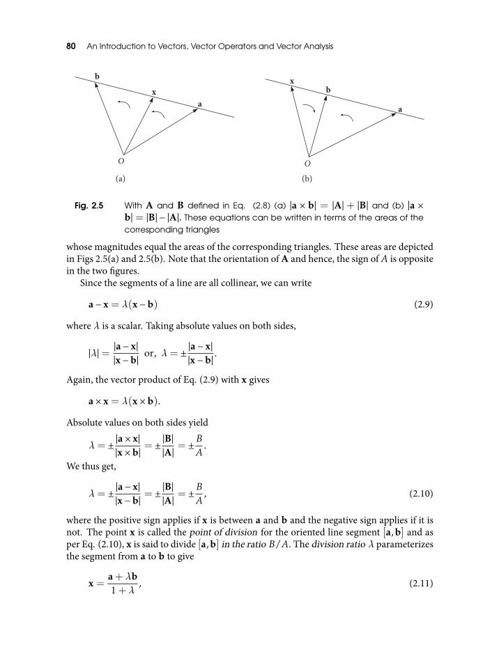
80 An Introduction to Vectors, Vector Operators and Vector Analysis
Fig. 2.5 With A and B defined in Eq. (2.8) (a) |a × b| = |A| + |B| and (b) |a ×b| = |B| − |A|. These equations can be written in terms of the areas of thecorresponding triangles
whose magnitudes equal the areas of the corresponding triangles. These areas are depictedin Figs 2.5(a) and 2.5(b). Note that the orientation of A and hence, the sign ofA is oppositein the two figures.
Since the segments of a line are all collinear, we can write
a− x = λ(x−b) (2.9)
where λ is a scalar. Taking absolute values on both sides,
|λ|= |a− x||x−b|
or, λ= ± |a− x||x−b|
.
Again, the vector product of Eq. (2.9) with x gives
a× x = λ(x×b).
Absolute values on both sides yield
λ= ± |a× x||x×b|
= ± |B||A|
= ±BA
.
We thus get,
λ= ± |a− x||x−b|
= ± |B||A|
= ±BA
, (2.10)
where the positive sign applies if x is between a and b and the negative sign applies if it isnot. The point x is called the point of division for the oriented line segment [a,b] and asper Eq. (2.10), x is said to divide [a,b] in the ratio B/A. The division ratio λ parameterizesthe segment from a to b to give
x =a+λb1+λ
, (2.11)
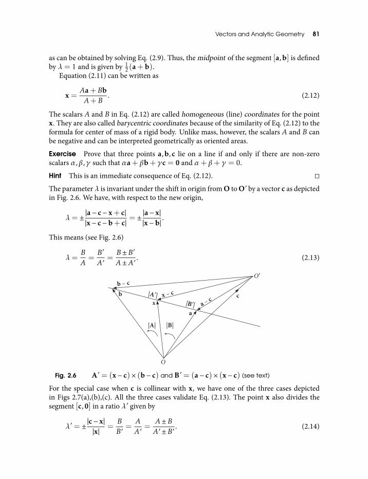
Vectors and Analytic Geometry 81
as can be obtained by solving Eq. (2.9). Thus, the midpoint of the segment [a,b] is definedby λ= 1 and is given by 1
2(a+b).Equation (2.11) can be written as
x =Aa+BbA+B
. (2.12)
The scalars A and B in Eq. (2.12) are called homogeneous (line) coordinates for the pointx. They are also called barycentric coordinates because of the similarity of Eq. (2.12) to theformula for center of mass of a rigid body. Unlike mass, however, the scalars A and B canbe negative and can be interpreted geometrically as oriented areas.
Exercise Prove that three points a,b,c lie on a line if and only if there are non-zeroscalars α,β,γ such that αa+ βb+ γc = 0 and α+ β+ γ = 0.
Hint This is an immediate consequence of Eq. (2.12).
The parameterλ is invariant under the shift in origin from O to O′ by a vector c as depictedin Fig. 2.6. We have, with respect to the new origin,
λ= ± |a− c− x+ c||x− c−b+ c|
= ± |a− x||x−b|
.
This means (see Fig. 2.6)
λ=BA
=B′
A′=B±B′
A±A′. (2.13)
Fig. 2.6 A′ = (x− c)× (b− c) and B′ = (a− c)× (x− c) (see text)
For the special case when c is collinear with x, we have one of the three cases depictedin Figs 2.7(a),(b),(c). All the three cases validate Eq. (2.13). The point x also divides thesegment [c,0] in a ratio λ′ given by
λ′ = ±|c− x||x|
=BB′
=AA′
=A±BA′ ±B′
. (2.14)
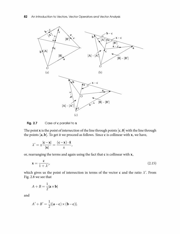
82 An Introduction to Vectors, Vector Operators and Vector Analysis
Fig. 2.7 Case of c parallel to x
The point x is the point of intersection of the line through points [c,0] with the line throughthe points [a,b]. To get it we proceed as follows. Since c is collinear with x, we have,
λ′ = ±|c− x||x|
=(c− x) · x
x,
or, rearranging the terms and again using the fact that c is collinear with x,
x =c
1+λ′, (2.15)
which gives us the point of intersection in terms of the vector c and the ratio λ′. FromFig. 2.8 we see that
A+B=12|a×b|
and
A′ +B′ =12|(a− c)× (b− c)|.
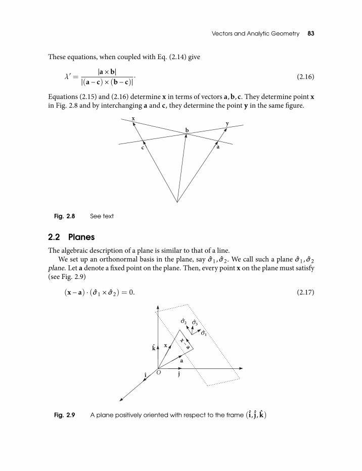
Vectors and Analytic Geometry 83
These equations, when coupled with Eq. (2.14) give
λ′ =|a×b|
|(a− c)× (b− c)|· (2.16)
Equations (2.15) and (2.16) determine x in terms of vectors a,b,c. They determine point xin Fig. 2.8 and by interchanging a and c, they determine the point y in the same figure.
Fig. 2.8 See text
2.2 PlanesThe algebraic description of a plane is similar to that of a line.
We set up an orthonormal basis in the plane, say σ1, σ2. We call such a plane σ1, σ2plane. Let a denote a fixed point on the plane. Then, every point x on the plane must satisfy(see Fig. 2.9)
(x− a) · (σ1 × σ2) = 0. (2.17)
Fig. 2.9 A plane positively oriented with respect to the frame (i, j, k)
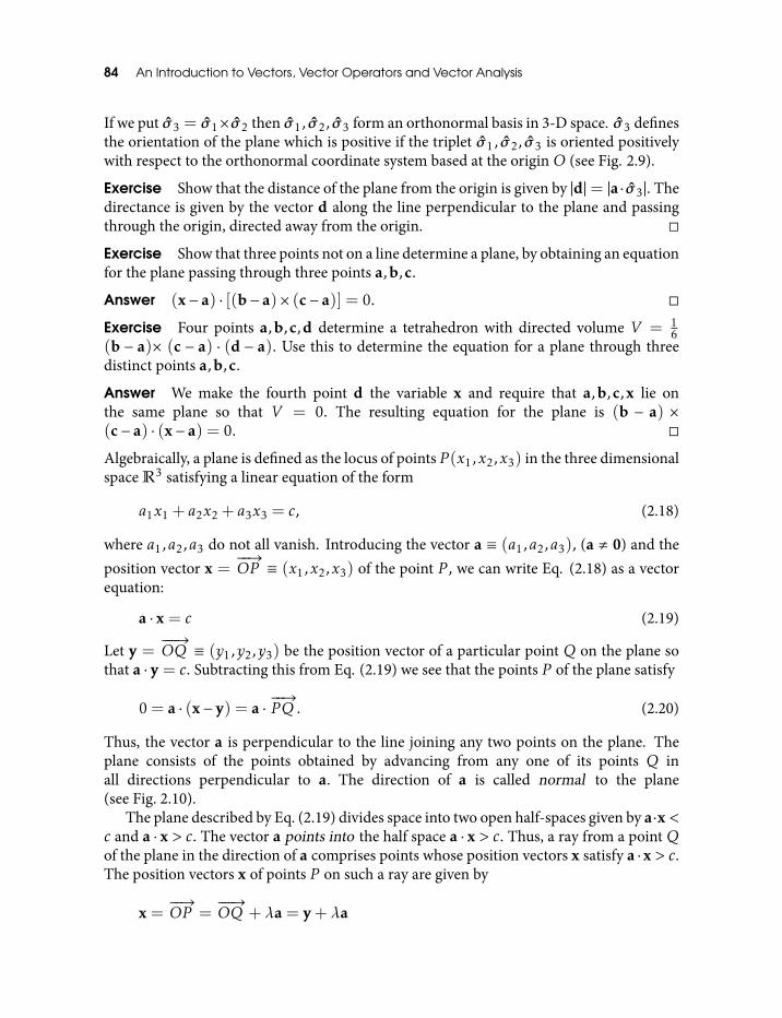
84 An Introduction to Vectors, Vector Operators and Vector Analysis
If we put σ3 = σ1×σ2 then σ1, σ2, σ3 form an orthonormal basis in 3-D space. σ3 definesthe orientation of the plane which is positive if the triplet σ1, σ2, σ3 is oriented positivelywith respect to the orthonormal coordinate system based at the originO (see Fig. 2.9).
Exercise Show that the distance of the plane from the origin is given by |d|= |a ·σ3|. Thedirectance is given by the vector d along the line perpendicular to the plane and passingthrough the origin, directed away from the origin.
Exercise Show that three points not on a line determine a plane, by obtaining an equationfor the plane passing through three points a,b,c.
Answer (x− a) · [(b− a)× (c− a)] = 0.
Exercise Four points a,b,c,d determine a tetrahedron with directed volume V = 16
(b − a)× (c − a) · (d − a). Use this to determine the equation for a plane through threedistinct points a,b,c.
Answer We make the fourth point d the variable x and require that a,b,c,x lie onthe same plane so that V = 0. The resulting equation for the plane is (b − a) ×(c− a) · (x− a) = 0.
Algebraically, a plane is defined as the locus of points P (x1,x2,x3) in the three dimensionalspace R3 satisfying a linear equation of the form
a1x1 + a2x2 + a3x3 = c, (2.18)
where a1,a2,a3 do not all vanish. Introducing the vector a ≡ (a1,a2,a3), (a , 0) and theposition vector x =
−−→OP ≡ (x1,x2,x3) of the point P , we can write Eq. (2.18) as a vector
equation:
a · x = c (2.19)
Let y =−−−→OQ ≡ (y1,y2,y3) be the position vector of a particular point Q on the plane so
that a · y = c. Subtracting this from Eq. (2.19) we see that the points P of the plane satisfy
0 = a · (x− y) = a ·−−→PQ . (2.20)
Thus, the vector a is perpendicular to the line joining any two points on the plane. Theplane consists of the points obtained by advancing from any one of its points Q inall directions perpendicular to a. The direction of a is called normal to the plane(see Fig. 2.10).
The plane described by Eq. (2.19) divides space into two open half-spaces given by a·x <c and a · x > c. The vector a points into the half space a · x > c. Thus, a ray from a point Qof the plane in the direction of a comprises points whose position vectors x satisfy a ·x > c.The position vectors x of points P on such a ray are given by
x =−−→OP =
−−−→OQ +λa = y+λa
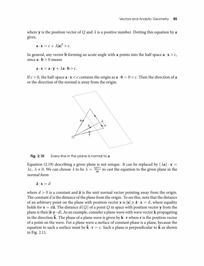
Vectors and Analytic Geometry 85
where y is the position vector of Q and λ is a positive number. Dotting this equation by agives,
a · x = c+λ|a|2 > c.
In general, any vector b forming an acute angle with a points into the half space a · x > c,since a ·b > 0 means
a · x = a · y+λa ·b > c.
If c > 0, the half-space a · x < c contains the origin as a · 0 = 0 < c. Then the direction of aor the direction of the normal is away from the origin.
Fig. 2.10 Every line in the plane is normal to a
Equation (2.19) describing a given plane is not unique. It can be replaced by (λa) · x =λc, λ , 0. We can choose λ to be λ =
sgn c|a| to cast the equation to the given plane in the
normal form
a · x = d
where d > 0 is a constant and a is the unit normal vector pointing away from the origin.The constant d is the distance of the plane from the origin. To see this, note that the distanceof an arbitrary point on the plane with position vector x is |x| ≥ a · x = d, where equalityholds for x = da. The distance d(Q) of a pointQ in space with position vector y from theplane is then |a·y−d|. As an example, consider a plane wave with wave vector k propagatingin the direction k. The phase of a plane wave is given by k · r where r is the position vectorof a point on the wave. For a plane wave a surface of constant phase is a plane, because theequation to such a surface must be k · r = c. Such a plane is perpendicular to k as shownin Fig. 2.11.
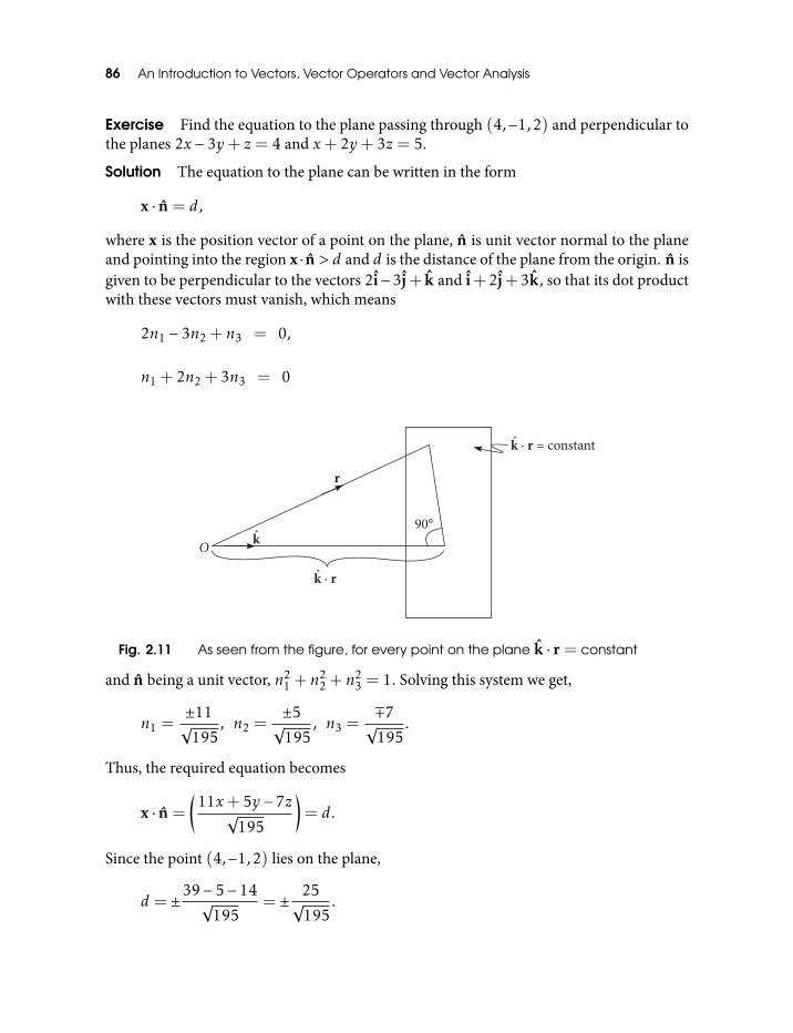
86 An Introduction to Vectors, Vector Operators and Vector Analysis
Exercise Find the equation to the plane passing through (4,−1,2) and perpendicular tothe planes 2x − 3y+ z = 4 and x+ 2y+ 3z = 5.
Solution The equation to the plane can be written in the form
x · n = d,
where x is the position vector of a point on the plane, n is unit vector normal to the planeand pointing into the region x · n > d and d is the distance of the plane from the origin. n isgiven to be perpendicular to the vectors 2i−3j+ k and i+2j+3k, so that its dot productwith these vectors must vanish, which means
2n1 − 3n2 + n3 = 0,
n1 + 2n2 + 3n3 = 0
Fig. 2.11 As seen from the figure, for every point on the plane k · r = constant
and n being a unit vector, n21 + n
22 + n
23 = 1. Solving this system we get,
n1 =±11√
195, n2 =
±5√
195, n3 =
∓7√
195.
Thus, the required equation becomes
x · n =
(11x+ 5y − 7z√
195
)= d.
Since the point (4,−1,2) lies on the plane,
d = ±39− 5− 14√
195= ± 25√
195.
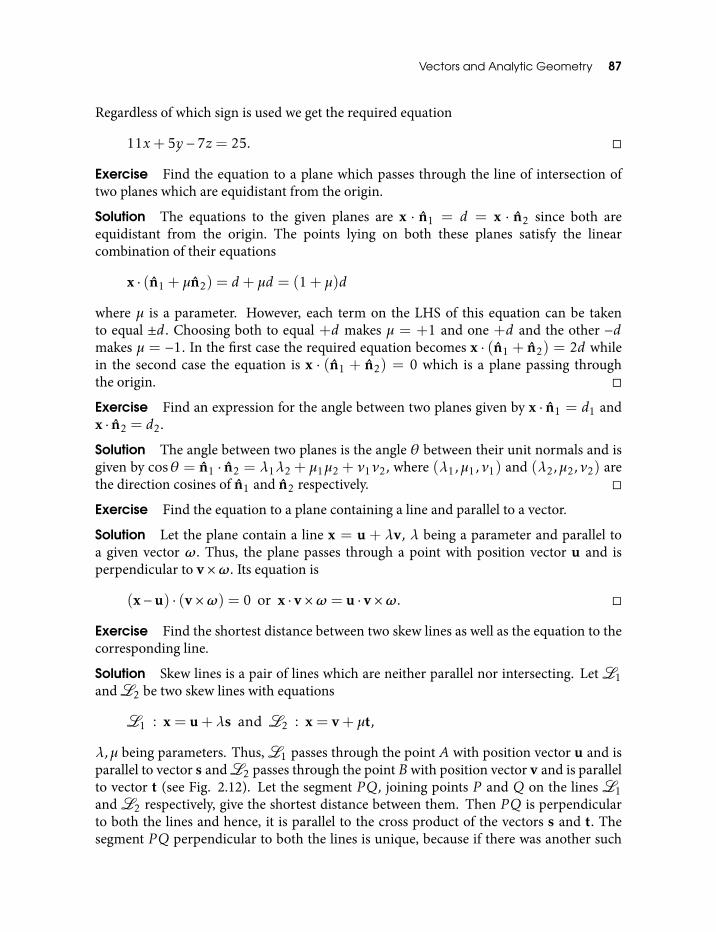
Vectors and Analytic Geometry 87
Regardless of which sign is used we get the required equation
11x+ 5y − 7z = 25.
Exercise Find the equation to a plane which passes through the line of intersection oftwo planes which are equidistant from the origin.
Solution The equations to the given planes are x · n1 = d = x · n2 since both areequidistant from the origin. The points lying on both these planes satisfy the linearcombination of their equations
x · (n1 + µn2) = d+ µd = (1+ µ)d
where µ is a parameter. However, each term on the LHS of this equation can be takento equal ±d. Choosing both to equal +d makes µ = +1 and one +d and the other −dmakes µ = −1. In the first case the required equation becomes x · (n1 + n2) = 2d whilein the second case the equation is x · (n1 + n2) = 0 which is a plane passing throughthe origin.
Exercise Find an expression for the angle between two planes given by x · n1 = d1 andx · n2 = d2.
Solution The angle between two planes is the angle θ between their unit normals and isgiven by cosθ = n1 · n2 = λ1λ2 + µ1µ2 + ν1ν2, where (λ1,µ1,ν1) and (λ2,µ2,ν2) arethe direction cosines of n1 and n2 respectively.
Exercise Find the equation to a plane containing a line and parallel to a vector.
Solution Let the plane contain a line x = u + λv, λ being a parameter and parallel toa given vector ω. Thus, the plane passes through a point with position vector u and isperpendicular to v×ω. Its equation is
(x−u) · (v×ω) = 0 or x · v×ω = u · v×ω.
Exercise Find the shortest distance between two skew lines as well as the equation to thecorresponding line.
Solution Skew lines is a pair of lines which are neither parallel nor intersecting. Let L1andL2 be two skew lines with equations
L1 : x = u+λs and L2 : x = v+ µt,
λ,µ being parameters. Thus,L1 passes through the point A with position vector u and isparallel to vector s andL2 passes through the point B with position vector v and is parallelto vector t (see Fig. 2.12). Let the segment PQ, joining points P and Q on the lines L1and L2 respectively, give the shortest distance between them. Then PQ is perpendicularto both the lines and hence, it is parallel to the cross product of the vectors s and t. Thesegment PQ perpendicular to both the lines is unique, because if there was another such
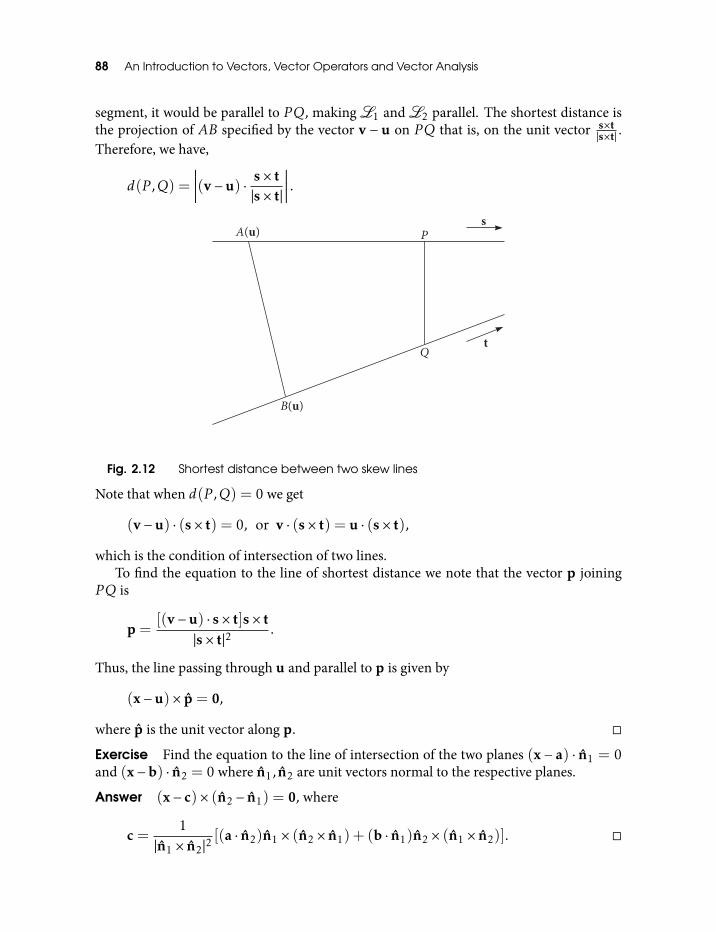
88 An Introduction to Vectors, Vector Operators and Vector Analysis
segment, it would be parallel to PQ, makingL1 andL2 parallel. The shortest distance isthe projection of AB specified by the vector v − u on PQ that is, on the unit vector s×t
|s×t| .Therefore, we have,
d(P ,Q) =∣∣∣∣∣(v−u) · s× t
|s× t|
∣∣∣∣∣ .
Fig. 2.12 Shortest distance between two skew lines
Note that when d(P ,Q) = 0 we get
(v−u) · (s× t) = 0, or v · (s× t) = u · (s× t),
which is the condition of intersection of two lines.To find the equation to the line of shortest distance we note that the vector p joining
PQ is
p =[(v−u) · s× t]s× t
|s× t|2.
Thus, the line passing through u and parallel to p is given by
(x−u)× p = 0,
where p is the unit vector along p.
Exercise Find the equation to the line of intersection of the two planes (x − a) · n1 = 0and (x−b) · n2 = 0 where n1, n2 are unit vectors normal to the respective planes.
Answer (x− c)× (n2 − n1) = 0, where
c =1
|n1 × n2|2[(a · n2)n1 × (n2 × n1) + (b · n1)n2 × (n1 × n2)].
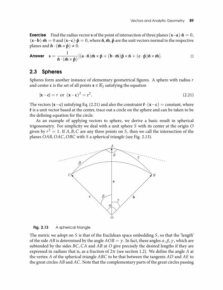
Vectors and Analytic Geometry 89
Exercise Find the radius vector s of the point of intersection of three planes (x−a)·n = 0,(x−b)·m = 0 and (x−c)·p = 0, where n,m, p are the unit vectors normal to the respectiveplanes and n · (m× p) , 0.
Answer s =1
n · (m× p)[(a · n)m× p+ (b · m)p× n+ (c · p)n× m].
2.3 SpheresSpheres form another instance of elementary geometrical figures. A sphere with radius rand center c is the set of all points x ∈ E3 satisfying the equation
|x− c|= r or (x− c)2 = r2. (2.21)
The vectors x−c satisfying Eq. (2.21) and also the constraint r · (x−c) = constant, wherer is a unit vector based at the center, trace out a circle on the sphere and can be taken to bethe defining equation for the circle.
As an example of applying vectors to sphere, we derive a basic result in sphericaltrigonometry. For simplicity we deal with a unit sphere S with its center at the origin Ogiven by r2 = 1. If A,B,C are any three points on S, then we call the intersection of theplanesOAB,OAC,OBC with S a spherical triangle (see Fig. 2.13).
Fig. 2.13 A spherical triangle
The metric we adopt on S is that of the Euclidean space embedding S, so that the ‘length’of the sideAB is determined by the angleAOB= γ . In fact, these angles α,β,γ , which aresubtended by the sides BC,CA and AB at O give precisely the desired lengths if they areexpressed in radians that is, as a fraction of 2π (see section 1.2). We define the angle A atthe vertex A of the spherical triangle ABC to be that between the tangents AD and AE tothe great circlesAB andAC. Note that the complementary parts of the great circles passing
90 An Introduction to Vectors, Vector Operators and Vector Analysis
through AB,BC and CA also form a spherical triangle ABC. We can specify the trianglein Fig. 2.13 by requiring that every angle of the triangle ABC has to be less than π.
We wish to prove the identity
cosα = cosγ cosβ+ sinγ sinβ cosA.
To this end we use identity II by replacing c by a and d by c. We get, remembering that allvectors are unit vectors,
(a× b) · (a× c) = (b · c)− (a · c)(b · a).
The angle between (a× b) and (a× c) is the dihedral angle between the planes OAC andOAB, that is, angle A. Further,
|a× b| = sinγ ,
|a× c| = sinβ,
(a× b) · (a× c) = sinγ sinβ cosA,
b · c = cosα,
(a · b)(a · c) = cosγ cosβ.
which gives the required result.
Exercise Show that, for a spherical triangle ABC, as in Fig. 2.13.,
sinAsinα
=sinBsinβ
=sinCsinγ
=σ
sinα sinβ sinγ,
where
σ = 2[sins sin(s −α)sin(s −α)sin(s −α)]1/2 ; s = α+ β+ γ .
Hint First get |(a × b) × (a × c)| = |a × b||a × c|sinA = sinγ sinβ sinA. Then evaluate|(a×b)×(a×c)| differently to obtain a quantity σ which is invarient under any permutationof vectors a, b, c.
2.4 Conic SectionsNext we consider an important set of planar curves called conic sections because each oneof them can be obtained as an intersection of a cone with a plane.
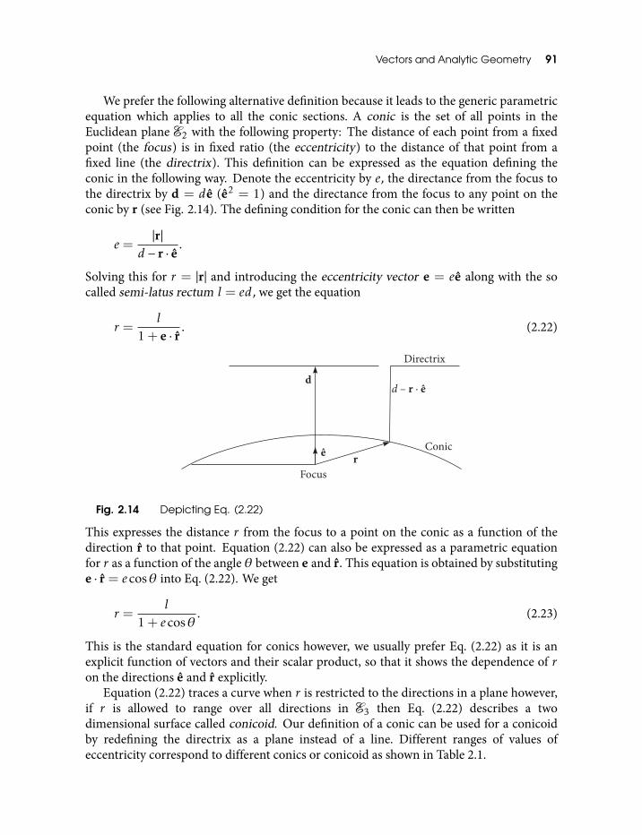
Vectors and Analytic Geometry 91
We prefer the following alternative definition because it leads to the generic parametricequation which applies to all the conic sections. A conic is the set of all points in theEuclidean plane E2 with the following property: The distance of each point from a fixedpoint (the focus) is in fixed ratio (the eccentricity) to the distance of that point from afixed line (the directrix). This definition can be expressed as the equation defining theconic in the following way. Denote the eccentricity by e, the directance from the focus tothe directrix by d = de (e2 = 1) and the directance from the focus to any point on theconic by r (see Fig. 2.14). The defining condition for the conic can then be written
e =|r|
d − r · e.
Solving this for r = |r| and introducing the eccentricity vector e = ee along with the socalled semi-latus rectum l = ed, we get the equation
r =l
1+ e · r. (2.22)
Fig. 2.14 Depicting Eq. (2.22)
This expresses the distance r from the focus to a point on the conic as a function of thedirection r to that point. Equation (2.22) can also be expressed as a parametric equationfor r as a function of the angle θ between e and r. This equation is obtained by substitutinge · r = ecosθ into Eq. (2.22). We get
r =l
1+ ecosθ. (2.23)
This is the standard equation for conics however, we usually prefer Eq. (2.22) as it is anexplicit function of vectors and their scalar product, so that it shows the dependence of ron the directions e and r explicitly.
Equation (2.22) traces a curve when r is restricted to the directions in a plane however,if r is allowed to range over all directions in E3 then Eq. (2.22) describes a twodimensional surface called conicoid. Our definition of a conic can be used for a conicoidby redefining the directrix as a plane instead of a line. Different ranges of values ofeccentricity correspond to different conics or conicoid as shown in Table 2.1.
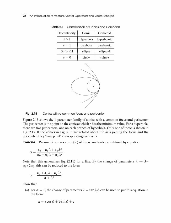
92 An Introduction to Vectors, Vector Operators and Vector Analysis
Table 2.1 Classification of Conics and Conicoids
Eccentricity Conic Conicoid
e > 1 Hyperbola hyperboloid
e = 1 parabola paraboloid
0 < e < 1 ellipse ellipsoid
e = 0 circle sphere
Fig. 2.15 Conics with a common focus and pericenter
Figure 2.15 shows the 1-parameter family of conics with a common focus and pericenter.The pericenter is the point on the conic at which r has the minimum value. For a hyperbola,there are two pericenters, one on each branch of hyperbola. Only one of these is shown inFig. 2.15. If the conics in Fig. 2.15 are rotated about the axis joining the focus and thepericenter, they “sweep out” corresponding conicoids.
Exercise Parametric curves x = x(λ) of the second order are defined by equation
x =a0 + a1λ+ a2λ
2
α0 +α1λ+α2λ2 .
Note that this generalizes Eq. (2.11) for a line. By the change of parameters λ → λ−α1/2α2, this can be reduced to the form
x =a0 + a1λ+ a2λ
2
α+λ2 .
Show that
(a) For α = 1, the change of parameters λ= tan 12φ can be used to put this equation in
the form
x = acosφ+bsinφ+ c
Vectors and Analytic Geometry 93
which is the general equation for an ellipse.(b) For α = −1, λ= tanh 1
2φ gives
x = acoshφ+bsinhφ+ c.
which is the general equation for a hyperbola.
Actually ultimate conclusion you can draw turns out to be true: All conics are secondorder curves and conversely.
Hint (a)mf a0 = a+ c, a1 = 2b, a2 = c− a cosφ = 1−λ2
1+λ2 , sinφ = 2λ1+λ2 .
Conics and conicoids can be described in many different ways which disclose a variety oftheir remarkable properties. However, any discussion of these issues will take us far awayfrom the main theme of this book. These are discussed at length in various books onmechanics and geometry [9, 18].
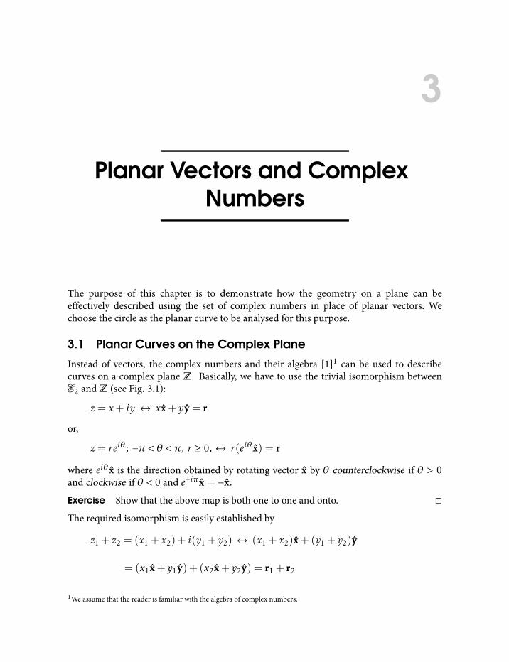
3
Planar Vectors and ComplexNumbers
The purpose of this chapter is to demonstrate how the geometry on a plane can beeffectively described using the set of complex numbers in place of planar vectors. Wechoose the circle as the planar curve to be analysed for this purpose.
3.1 Planar Curves on the Complex Plane
Instead of vectors, the complex numbers and their algebra [1]1 can be used to describecurves on a complex plane Z. Basically, we have to use the trivial isomorphism betweenE2 and Z (see Fig. 3.1):
z = x+ iy ↔ xx+ yy = r
or,
z = reiθ; −π < θ < π, r ≥ 0, ↔ r(eiθx) = r
where eiθx is the direction obtained by rotating vector x by θ counterclockwise if θ > 0and clockwise if θ < 0 and e±iπx = −x.
Exercise Show that the above map is both one to one and onto.
The required isomorphism is easily established by
z1 + z2 = (x1 + x2) + i(y1 + y2) ↔ (x1 + x2)x+ (y1 + y2)y
= (x1x+ y1y) + (x2x+ y2y) = r1 + r2
1We assume that the reader is familiar with the algebra of complex numbers.
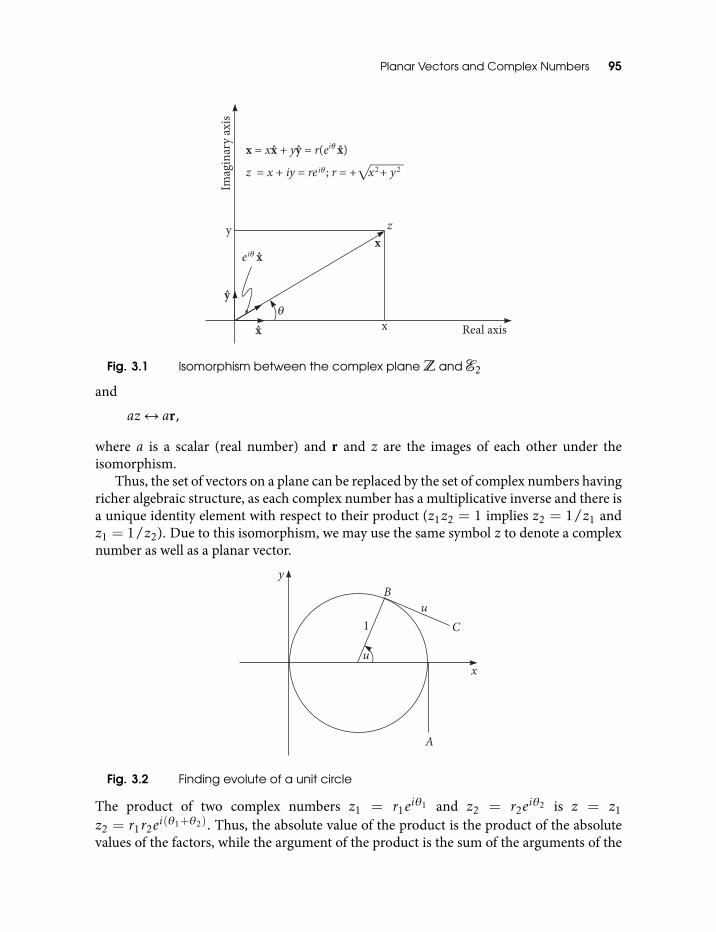
Planar Vectors and Complex Numbers 95
Fig. 3.1 Isomorphism between the complex plane Z and E2
and
az↔ ar,
where a is a scalar (real number) and r and z are the images of each other under theisomorphism.
Thus, the set of vectors on a plane can be replaced by the set of complex numbers havingricher algebraic structure, as each complex number has a multiplicative inverse and there isa unique identity element with respect to their product (z1z2 = 1 implies z2 = 1/z1 andz1 = 1/z2). Due to this isomorphism, we may use the same symbol z to denote a complexnumber as well as a planar vector.
Fig. 3.2 Finding evolute of a unit circle
The product of two complex numbers z1 = r1eiθ1 and z2 = r2e
iθ2 is z = z1z2 = r1r2e
i(θ1+θ2). Thus, the absolute value of the product is the product of the absolutevalues of the factors, while the argument of the product is the sum of the arguments of the
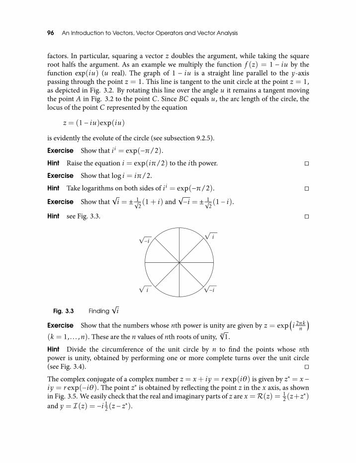
96 An Introduction to Vectors, Vector Operators and Vector Analysis
factors. In particular, squaring a vector z doubles the argument, while taking the squareroot halfs the argument. As an example we multiply the function f (z) = 1 − iu by thefunction exp(iu) (u real). The graph of 1 − iu is a straight line parallel to the y-axispassing through the point z = 1. This line is tangent to the unit circle at the point z = 1,as depicted in Fig. 3.2. By rotating this line over the angle u it remains a tangent movingthe point A in Fig. 3.2 to the point C. Since BC equals u, the arc length of the circle, thelocus of the point C represented by the equation
z = (1− iu)exp(iu)
is evidently the evolute of the circle (see subsection 9.2.5).
Exercise Show that ii = exp(−π/2).
Hint Raise the equation i = exp(iπ/2) to the ith power.
Exercise Show that log i = iπ/2.
Hint Take logarithms on both sides of ii = exp(−π/2).
Exercise Show that√i = ± 1√
2(1+ i) and
√−i = ± 1√
2(1− i).
Hint see Fig. 3.3.
Fig. 3.3 Finding√i
Exercise Show that the numbers whose nth power is unity are given by z = exp(i 2πkn
)(k = 1, . . . ,n). These are the n values of nth roots of unity, n
√1.
Hint Divide the circumference of the unit circle by n to find the points whose nthpower is unity, obtained by performing one or more complete turns over the unit circle(see Fig. 3.4).
The complex conjugate of a complex number z = x+ iy = r exp(iθ) is given by z∗ = x −iy = r exp(−iθ). The point z∗ is obtained by reflecting the point z in the x axis, as shownin Fig. 3.5. We easily check that the real and imaginary parts of z are x =R(z) = 1
2(z+z∗)
and y = I (z) = −i 12(z − z
∗).
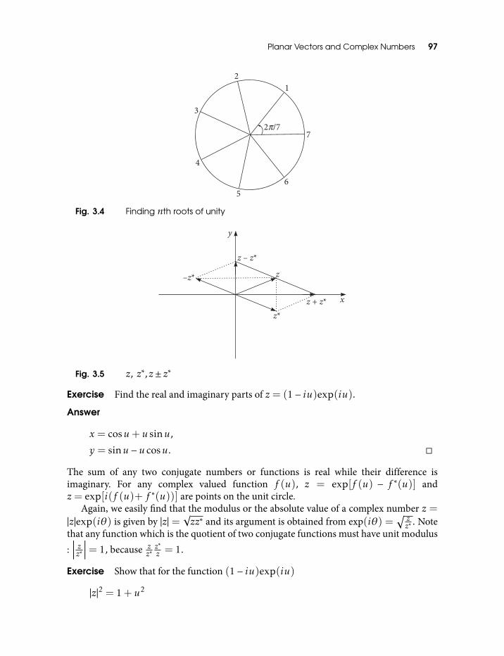
Planar Vectors and Complex Numbers 97
Fig. 3.4 Finding nth roots of unity
Fig. 3.5 z, z∗,z ± z∗
Exercise Find the real and imaginary parts of z = (1− iu)exp(iu).
Answer
x = cosu+ u sinu,
y = sinu −u cosu.
The sum of any two conjugate numbers or functions is real while their difference isimaginary. For any complex valued function f (u), z = exp[f (u) − f ∗(u)] andz = exp[i(f (u)+ f ∗(u))] are points on the unit circle.
Again, we easily find that the modulus or the absolute value of a complex number z =|z|exp(iθ) is given by |z| =
√zz∗ and its argument is obtained from exp(iθ) =
√zz∗ . Note
that any function which is the quotient of two conjugate functions must have unit modulus:∣∣∣∣ zz∗ ∣∣∣∣= 1, because z
z∗z∗z = 1.
Exercise Show that for the function (1− iu)exp(iu)
|z|2 = 1+ u2
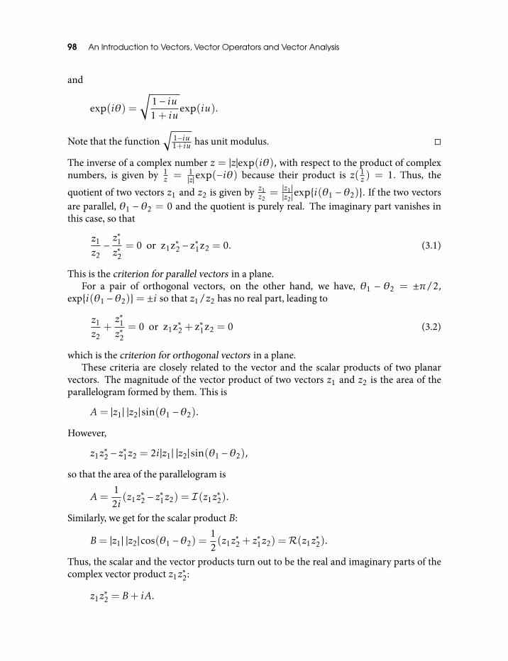
98 An Introduction to Vectors, Vector Operators and Vector Analysis
and
exp(iθ) =
√1− iu1+ iu
exp(iu).
Note that the function√
1−iu1+iu has unit modulus.
The inverse of a complex number z = |z|exp(iθ), with respect to the product of complexnumbers, is given by 1
z = 1|z|exp(−iθ) because their product is z(1
z ) = 1. Thus, the
quotient of two vectors z1 and z2 is given by z1z2
= |z1||z2|
expi(θ1 − θ2). If the two vectorsare parallel, θ1 − θ2 = 0 and the quotient is purely real. The imaginary part vanishes inthis case, so that
z1
z2−z∗1z∗2
= 0 or z1z∗2 − z∗1z2 = 0. (3.1)
This is the criterion for parallel vectors in a plane.For a pair of orthogonal vectors, on the other hand, we have, θ1 − θ2 = ±π/2,
expi(θ1 −θ2)= ±i so that z1/z2 has no real part, leading to
z1
z2+z∗1z∗2
= 0 or z1z∗2 + z∗1z2 = 0 (3.2)
which is the criterion for orthogonal vectors in a plane.These criteria are closely related to the vector and the scalar products of two planar
vectors. The magnitude of the vector product of two vectors z1 and z2 is the area of theparallelogram formed by them. This is
A= |z1| |z2|sin(θ1 −θ2).
However,
z1z∗2 − z
∗1z2 = 2i|z1| |z2|sin(θ1 −θ2),
so that the area of the parallelogram is
A=12i(z1z
∗2 − z
∗1z2) = I (z1z
∗2).
Similarly, we get for the scalar product B:
B= |z1| |z2|cos(θ1 −θ2) =12(z1z
∗2 + z
∗1z2) =R(z1z
∗2).
Thus, the scalar and the vector products turn out to be the real and imaginary parts of thecomplex vector product z1z
∗2:
z1z∗2 = B+ iA.
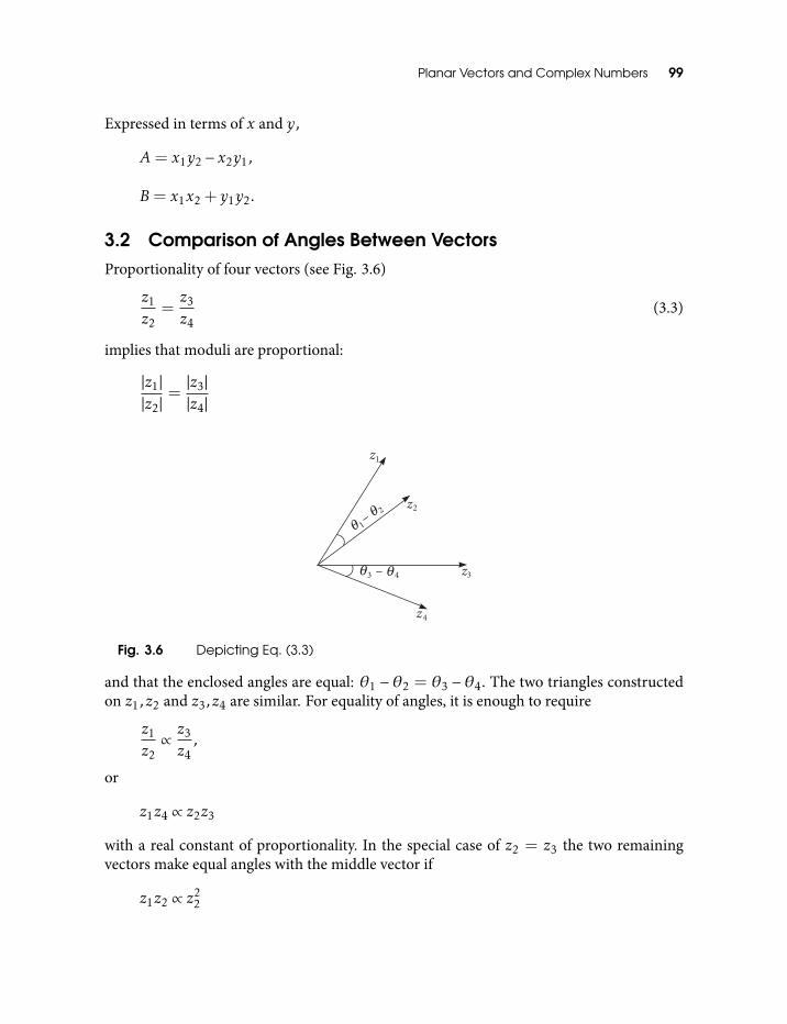
Planar Vectors and Complex Numbers 99
Expressed in terms of x and y,
A= x1y2 − x2y1,
B= x1x2 + y1y2.
3.2 Comparison of Angles Between VectorsProportionality of four vectors (see Fig. 3.6)
z1
z2=z3
z4(3.3)
implies that moduli are proportional:
|z1||z2|
=|z3||z4|
Fig. 3.6 Depicting Eq. (3.3)
and that the enclosed angles are equal: θ1 − θ2 = θ3 − θ4. The two triangles constructedon z1,z2 and z3,z4 are similar. For equality of angles, it is enough to require
z1
z2∝ z3
z4,
or
z1z4 ∝ z2z3
with a real constant of proportionality. In the special case of z2 = z3 the two remainingvectors make equal angles with the middle vector if
z1z2 ∝ z22
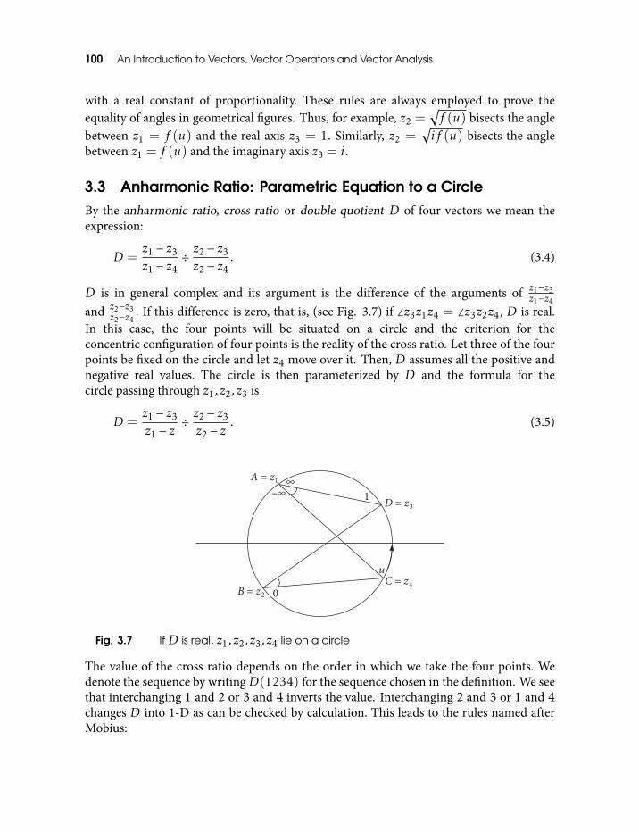
100 An Introduction to Vectors, Vector Operators and Vector Analysis
with a real constant of proportionality. These rules are always employed to prove theequality of angles in geometrical figures. Thus, for example, z2 =
√f (u) bisects the angle
between z1 = f (u) and the real axis z3 = 1. Similarly, z2 =√if (u) bisects the angle
between z1 = f (u) and the imaginary axis z3 = i.
3.3 Anharmonic Ratio: Parametric Equation to a CircleBy the anharmonic ratio, cross ratio or double quotient D of four vectors we mean theexpression:
D =z1 − z3
z1 − z4÷ z2 − z3
z2 − z4. (3.4)
D is in general complex and its argument is the difference of the arguments of z1−z3z1−z4
and z2−z3z2−z4
. If this difference is zero, that is, (see Fig. 3.7) if ∠z3z1z4 = ∠z3z2z4, D is real.In this case, the four points will be situated on a circle and the criterion for theconcentric configuration of four points is the reality of the cross ratio. Let three of the fourpoints be fixed on the circle and let z4 move over it. Then, D assumes all the positive andnegative real values. The circle is then parameterized by D and the formula for thecircle passing through z1,z2,z3 is
D =z1 − z3
z1 − z÷ z2 − z3
z2 − z. (3.5)
Fig. 3.7 If D is real, z1,z2,z3,z4 lie on a circle
The value of the cross ratio depends on the order in which we take the four points. Wedenote the sequence by writingD(1234) for the sequence chosen in the definition. We seethat interchanging 1 and 2 or 3 and 4 inverts the value. Interchanging 2 and 3 or 1 and 4changes D into 1-D as can be checked by calculation. This leads to the rules named afterMobius:
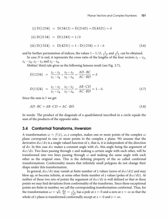
Planar Vectors and Complex Numbers 101
(i) D(1234) = D(3412) = D(2143) = D(4321) = δ
(ii) D(2134) = D(1243) = 1/δ
(iii) D(1324) = D(4231) = 1−D(1234) = 1− δ (3.6)
and by further permutation of indices, the values 1− 1/δ, 11−δ and δ
δ−1 can be obtained.In case D is real, it represents the cross ratio of the lengths of the four vectors z1 − z3,
z1 − z4, z2 − z3 and z2 − z4.Mobius’ third rule gives us the following famous result (see Fig. 3.7),
D(1234) =z1 − z3
z1 − z4÷ z2 − z3
z2 − z4=AD ·BCAC ·BD
= δ
D(1324) =z1 − z2
z1 − z4÷ z3 − z2
z3 − z4=AB ·CDAC ·BD
= 1− δ. (3.7)
Since the sum is 1 we get
AD ·BC+AB ·CD = AC ·BD. (3.8)
In words: The product of the diagonals of a quadrilateral inscribed in a circle equals thesum of the products of the opposite sides.
3.4 Conformal Transforms, InversionA transformation ω = f (z), ω,z complex, makes one or more points of the complex ωplane correspond to one or more points to the complex z plane. We assume that thederivative dω/dz is a single valued function of z, that is, it is independent of the directionof dz. In this case dω makes a constant angle with dz, this angle being the argument ofdω/dz. Two lines passing through z and making a certain angle with each other, will betransformed into two lines passing through ω and making the same angle with eachother as the original ones. This is the defining property of the so called conformaltransformations. Conformality means that infinitely small polygons do not change theirshape under this transformation.
In general, dω/dz may vanish at finite number of z values (zeros of dω/dz) and mayblow up, or become infinite, at some other finite number of z values (poles of dω/dz). Atneither of these two sets of points the argument of dω/dz is well defined so that at thesepoints we may find deviations from conformality of the transforms. Since these exceptionalpoints are finite in number, we call the corresponding transformation conformal. Thus, forthe transformation ω =
√z, dωdz = 1
2√z
has a pole at z = 0 and a zero at z =∞ so that thewhole of z plane is transformed conformally except at z = 0 and z =∞.
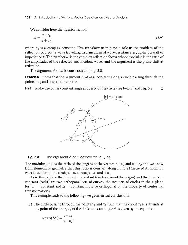
102 An Introduction to Vectors, Vector Operators and Vector Analysis
We consider here the transformation
ω =z − z0
z+ z0(3.9)
where z0 is a complex constant. This transformation plays a role in the problem of thereflection of a plane wave travelling in a medium of wave-resistance z0, against a wall ofimpedance z. The numberω is the complex reflection factor whose modulus is the ratio ofthe amplitudes of the reflected and incident waves and the argument is the phase shift atreflection.
The argument ∆ of ω is constructed in Fig. 3.8.
Exercise Show that the argument ∆ of ω is constant along a circle passing through thepoints −z0 and +z0 of the z plane.
Hint Make use of the constant angle property of the circle (see below) and Fig. 3.8.
Fig. 3.8 The argument ∆ of ω defined by Eq. (3.9)
The modulus of ω is the ratio of the lengths of the vectors z − z0 and z+ z0 and we knowfrom elementary geometry that this ratio is constant along a circle (Circle of Apollonius)with its center on the straight line through −z0 and +z0.
As in the ω plane the lines |ω|= constant (circles around the origin) and the lines ∆=constant (radii) are two orthogonal sets of curves, the two sets of circles in the z planefor |ω| = constant and ∆ = constant must be orthogonal by the property of conformaltransformations.
This example leads to the following two geometrical conclusions:
(a) The circle passing through the points z1 and z2 such that the chord z1z2 subtends atany point of the arc z1z2 of the circle constant angle ∆ is given by the equation:
u exp(i∆) =z − z1
z − z2.
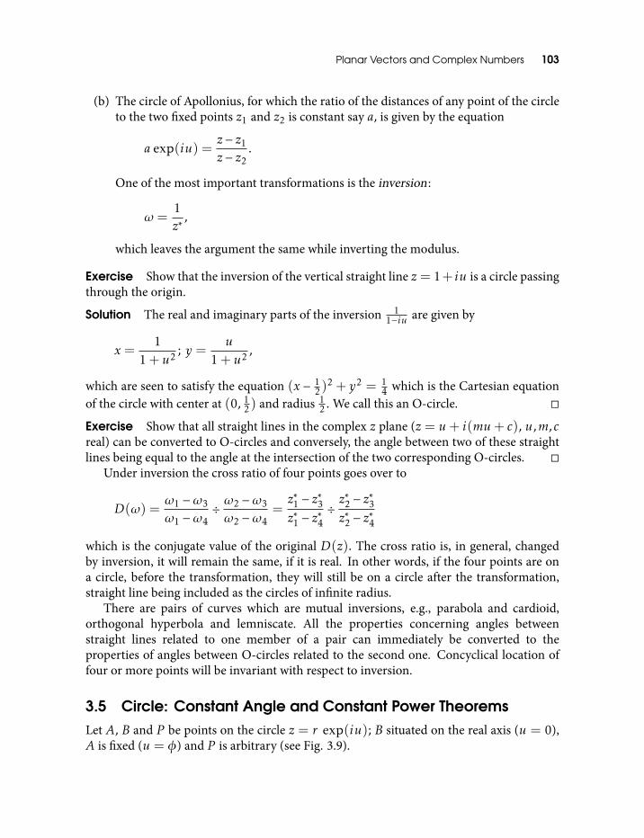
Planar Vectors and Complex Numbers 103
(b) The circle of Apollonius, for which the ratio of the distances of any point of the circleto the two fixed points z1 and z2 is constant say a, is given by the equation
a exp(iu) =z − z1
z − z2.
One of the most important transformations is the inversion :
ω =1z∗
,
which leaves the argument the same while inverting the modulus.
Exercise Show that the inversion of the vertical straight line z = 1+ iu is a circle passingthrough the origin.
Solution The real and imaginary parts of the inversion 11−iu are given by
x =1
1+ u2 ; y =u
1+ u2 ,
which are seen to satisfy the equation (x − 12)
2 + y2 = 14 which is the Cartesian equation
of the circle with center at (0, 12) and radius 1
2 . We call this an O-circle.
Exercise Show that all straight lines in the complex z plane (z = u+ i(mu+ c), u,m,creal) can be converted to O-circles and conversely, the angle between two of these straightlines being equal to the angle at the intersection of the two corresponding O-circles.
Under inversion the cross ratio of four points goes over to
D(ω) =ω1 −ω3
ω1 −ω4÷ ω2 −ω3
ω2 −ω4=z∗1 − z
∗3
z∗1 − z∗4÷z∗2 − z
∗3
z∗2 − z∗4
which is the conjugate value of the original D(z). The cross ratio is, in general, changedby inversion, it will remain the same, if it is real. In other words, if the four points are ona circle, before the transformation, they will still be on a circle after the transformation,straight line being included as the circles of infinite radius.
There are pairs of curves which are mutual inversions, e.g., parabola and cardioid,orthogonal hyperbola and lemniscate. All the properties concerning angles betweenstraight lines related to one member of a pair can immediately be converted to theproperties of angles between O-circles related to the second one. Concyclical location offour or more points will be invariant with respect to inversion.
3.5 Circle: Constant Angle and Constant Power TheoremsLet A, B and P be points on the circle z = r exp(iu); B situated on the real axis (u = 0),A is fixed (u = φ) and P is arbitrary (see Fig. 3.9).
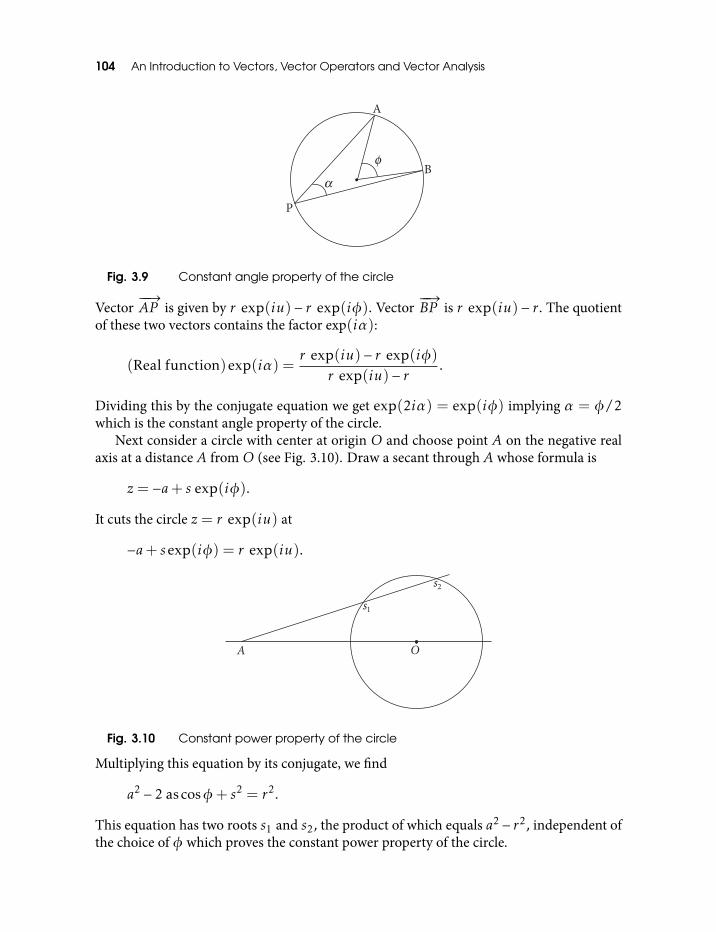
104 An Introduction to Vectors, Vector Operators and Vector Analysis
Fig. 3.9 Constant angle property of the circle
Vector−−→AP is given by r exp(iu)− r exp(iφ). Vector
−−→BP is r exp(iu)− r. The quotient
of these two vectors contains the factor exp(iα):
(Real function)exp(iα) =r exp(iu)− r exp(iφ)
r exp(iu)− r.
Dividing this by the conjugate equation we get exp(2iα) = exp(iφ) implying α = φ/2which is the constant angle property of the circle.
Next consider a circle with center at origin O and choose point A on the negative realaxis at a distance A fromO (see Fig. 3.10). Draw a secant through A whose formula is
z = −a+ s exp(iφ).
It cuts the circle z = r exp(iu) at
−a+ sexp(iφ) = r exp(iu).
Fig. 3.10 Constant power property of the circle
Multiplying this equation by its conjugate, we find
a2 − 2 ascosφ+ s2 = r2.
This equation has two roots s1 and s2, the product of which equals a2 − r2, independent ofthe choice of φ which proves the constant power property of the circle.
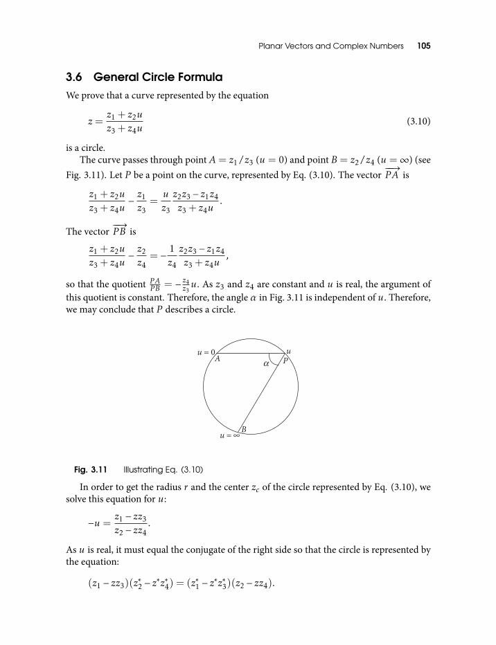
Planar Vectors and Complex Numbers 105
3.6 General Circle FormulaWe prove that a curve represented by the equation
z =z1 + z2uz3 + z4u
(3.10)
is a circle.The curve passes through point A= z1/z3 (u = 0) and point B= z2/z4 (u =∞) (see
Fig. 3.11). Let P be a point on the curve, represented by Eq. (3.10). The vector−−→PA is
z1 + z2uz3 + z4u
− z1
z3=uz3
z2z3 − z1z4
z3 + z4u.
The vector−−→P B is
z1 + z2uz3 + z4u
− z2
z4= − 1
z4
z2z3 − z1z4
z3 + z4u,
so that the quotient PAP B = − z4z3u. As z3 and z4 are constant and u is real, the argument of
this quotient is constant. Therefore, the angle α in Fig. 3.11 is independent of u. Therefore,we may conclude that P describes a circle.
Fig. 3.11 Illustrating Eq. (3.10)
In order to get the radius r and the center zc of the circle represented by Eq. (3.10), wesolve this equation for u:
−u =z1 − zz3
z2 − zz4.
As u is real, it must equal the conjugate of the right side so that the circle is represented bythe equation:
(z1 − zz3)(z∗2 − z
∗z∗4) = (z∗1 − z∗z∗3)(z2 − zz4).
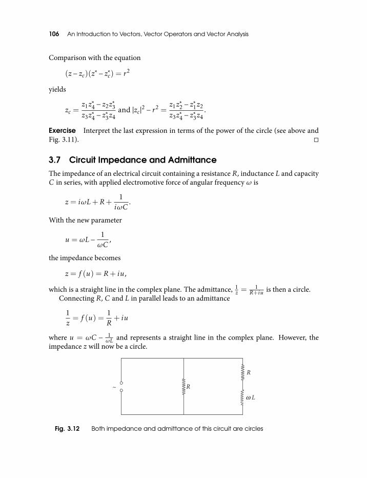
106 An Introduction to Vectors, Vector Operators and Vector Analysis
Comparison with the equation
(z − zc)(z∗ − z∗c) = r2
yields
zc =z1z∗4 − z2z
∗3
z3z∗4 − z
∗3z4
and |zc|2 − r2 =z1z∗2 − z
∗1z2
z3z∗4 − z
∗3z4
.
Exercise Interpret the last expression in terms of the power of the circle (see above andFig. 3.11).
3.7 Circuit Impedance and AdmittanceThe impedance of an electrical circuit containing a resistance R, inductance L and capacityC in series, with applied electromotive force of angular frequency ω is
z = iωL+R+1iωC
.
With the new parameter
u = ωL− 1ωC
,
the impedance becomes
z = f (u) = R+ iu,
which is a straight line in the complex plane. The admittance, 1z =
1R+iu is then a circle.
Connecting R, C and L in parallel leads to an admittance
1z= f (u) =
1R+ iu
where u = ωC − 1ωL and represents a straight line in the complex plane. However, the
impedance z will now be a circle.
Fig. 3.12 Both impedance and admittance of this circuit are circles
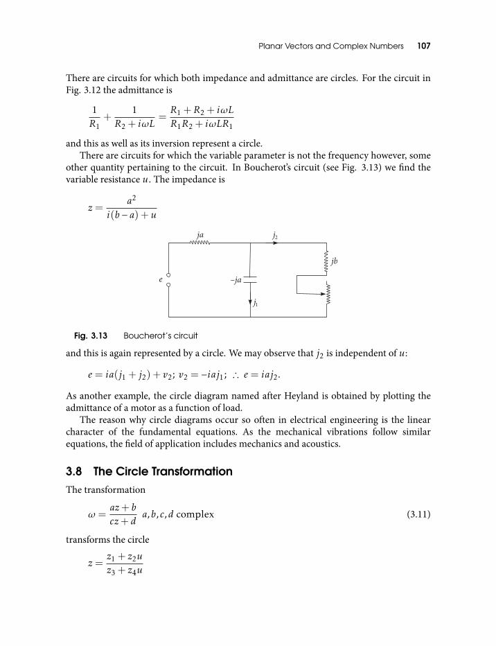
Planar Vectors and Complex Numbers 107
There are circuits for which both impedance and admittance are circles. For the circuit inFig. 3.12 the admittance is
1R1
+1
R2 + iωL=R1 +R2 + iωLR1R2 + iωLR1
and this as well as its inversion represent a circle.There are circuits for which the variable parameter is not the frequency however, some
other quantity pertaining to the circuit. In Boucherot’s circuit (see Fig. 3.13) we find thevariable resistance u. The impedance is
z =a2
i(b − a) + u
Fig. 3.13 Boucherot’s circuit
and this is again represented by a circle. We may observe that j2 is independent of u:
e = ia(j1 + j2) + v2; v2 = −iaj1; ∴ e = iaj2.
As another example, the circle diagram named after Heyland is obtained by plotting theadmittance of a motor as a function of load.
The reason why circle diagrams occur so often in electrical engineering is the linearcharacter of the fundamental equations. As the mechanical vibrations follow similarequations, the field of application includes mechanics and acoustics.
3.8 The Circle TransformationThe transformation
ω =az+ bcz+ d
a,b,c,d complex (3.11)
transforms the circle
z =z1 + z2uz3 + z4u
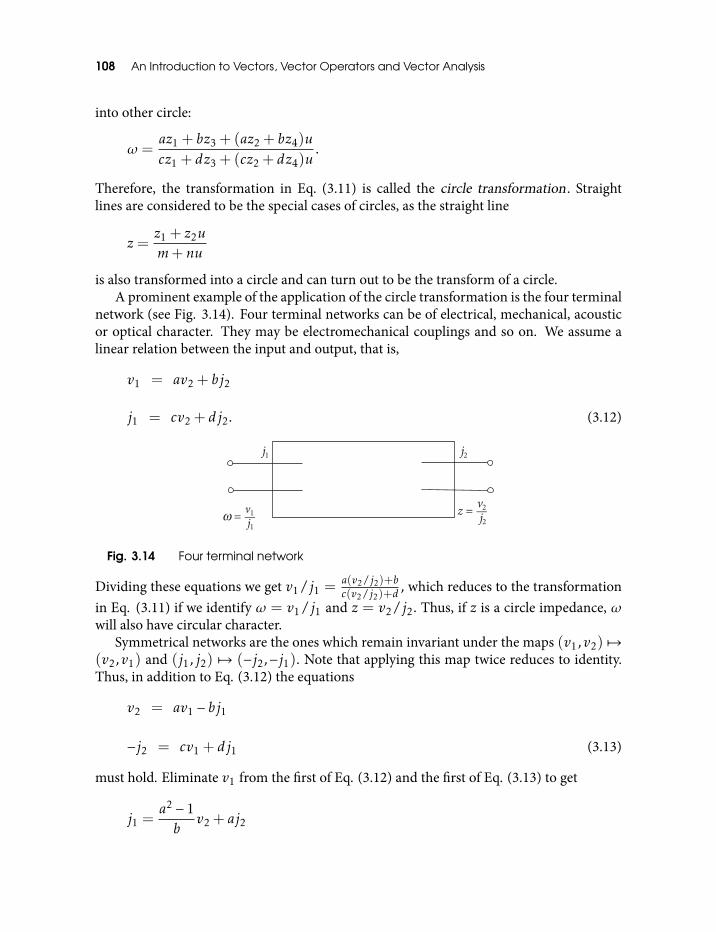
108 An Introduction to Vectors, Vector Operators and Vector Analysis
into other circle:
ω =az1 + bz3 + (az2 + bz4)u
cz1 + dz3 + (cz2 + dz4)u.
Therefore, the transformation in Eq. (3.11) is called the circle transformation . Straightlines are considered to be the special cases of circles, as the straight line
z =z1 + z2um+ nu
is also transformed into a circle and can turn out to be the transform of a circle.A prominent example of the application of the circle transformation is the four terminal
network (see Fig. 3.14). Four terminal networks can be of electrical, mechanical, acousticor optical character. They may be electromechanical couplings and so on. We assume alinear relation between the input and output, that is,
v1 = av2 + bj2
j1 = cv2 + dj2. (3.12)
Fig. 3.14 Four terminal network
Dividing these equations we get v1/j1 =a(v2/j2)+bc(v2/j2)+d
, which reduces to the transformationin Eq. (3.11) if we identify ω = v1/j1 and z = v2/j2. Thus, if z is a circle impedance, ωwill also have circular character.
Symmetrical networks are the ones which remain invariant under the maps (v1,v2) 7→(v2,v1) and (j1, j2) 7→ (−j2,−j1). Note that applying this map twice reduces to identity.Thus, in addition to Eq. (3.12) the equations
v2 = av1 − bj1
−j2 = cv1 + dj1 (3.13)
must hold. Eliminate v1 from the first of Eq. (3.12) and the first of Eq. (3.13) to get
j1 =a2 − 1b
v2 + aj2
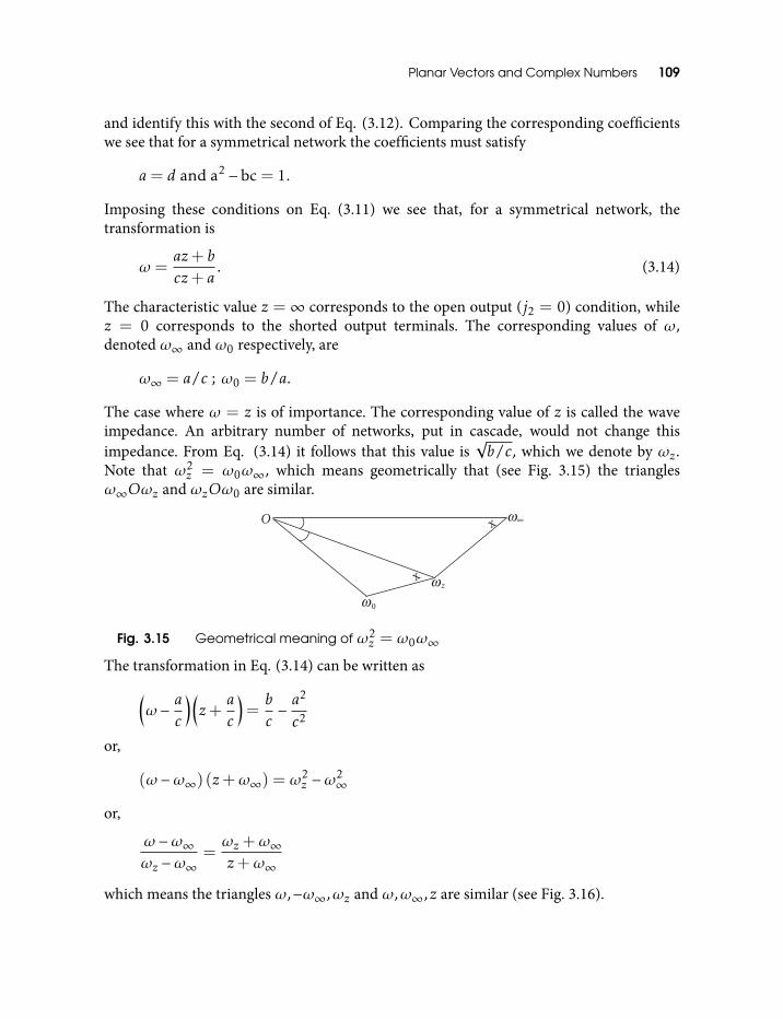
Planar Vectors and Complex Numbers 109
and identify this with the second of Eq. (3.12). Comparing the corresponding coefficientswe see that for a symmetrical network the coefficients must satisfy
a= d and a2 −bc = 1.
Imposing these conditions on Eq. (3.11) we see that, for a symmetrical network, thetransformation is
ω =az+ bcz+ a
. (3.14)
The characteristic value z = ∞ corresponds to the open output (j2 = 0) condition, whilez = 0 corresponds to the shorted output terminals. The corresponding values of ω,denoted ω∞ and ω0 respectively, are
ω∞ = a/c ; ω0 = b/a.
The case where ω = z is of importance. The corresponding value of z is called the waveimpedance. An arbitrary number of networks, put in cascade, would not change thisimpedance. From Eq. (3.14) it follows that this value is
√b/c, which we denote by ωz.
Note that ω2z = ω0ω∞, which means geometrically that (see Fig. 3.15) the triangles
ω∞Oωz and ωzOω0 are similar.
Fig. 3.15 Geometrical meaning of ω2z = ω0ω∞
The transformation in Eq. (3.14) can be written as(ω − a
c
)(z+
ac
)=bc− a
2
c2
or,
(ω −ω∞) (z+ω∞) = ω2z −ω2
∞
or,
ω −ω∞ωz −ω∞
=ωz+ω∞z+ω∞
which means the triangles ω,−ω∞,ωz and ω,ω∞,z are similar (see Fig. 3.16).
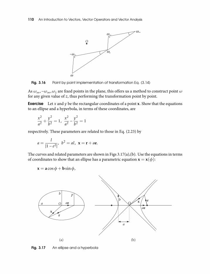
110 An Introduction to Vectors, Vector Operators and Vector Analysis
Fig. 3.16 Point by point implementation of transformation Eq. (3.14)
As ω∞,−ω∞,ωz are fixed points in the plane, this offers us a method to construct point ωfor any given value of z, thus performing the transformation point by point.
Exercise Let x and y be the rectangular coordinates of a point x. Show that the equationsto an ellipse and a hyperbola, in terms of these coordinates, are
x2
a2 +y2
b2 = 1,x2
a2 −y2
b2 = 1
respectively. These parameters are related to those in Eq. (2.23) by
a=l
|1− e2|, b2 = al, x = r+ ae.
The curves and related parameters are shown in Figs 3.17(a),(b). Use the equations in termsof coordinates to show that an ellipse has a parametric equation x = x(φ):
x = acosφ+bsinφ,
Fig. 3.17 An ellipse and a hyperbola
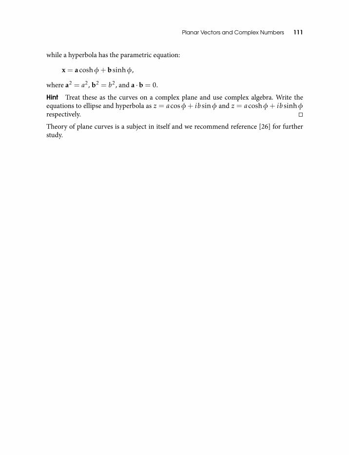
Planar Vectors and Complex Numbers 111
while a hyperbola has the parametric equation:
x = acoshφ+bsinhφ,
where a2 = a2, b2 = b2, and a ·b = 0.
Hint Treat these as the curves on a complex plane and use complex algebra. Write theequations to ellipse and hyperbola as z = acosφ+ ib sinφ and z = acoshφ+ ib sinhφrespectively.
Theory of plane curves is a subject in itself and we recommend reference [26] for furtherstudy.

Part II
Vector Operators
“My Lord! Please make me a cat!” prayed the mouse.— from a Panchatantra story

4
Linear Operators
4.1 Linear Operators on E3
We have seen that the fields are functions defined over the domain of position vectors orpoints in space and are either vector valued or scalar valued. We now consider functions(either vector valued or scalar valued) defined over some domain of vectors (not necessarilyposition vectors) with the additional requirement that the function be linear, that is,
f (αx+ βy) = αf (x) + βf (y),
where α and β are scalars. Such a function is called a linear operator, or operator forbrevity. In different contexts, such a function is also called a linear transformation or atensor. The term ‘tensor’ is used for describing certain properties of a physical system.Thus, the ‘inertia tensor’ is a property of a rigid body or the ‘strain tensor’ is a property ofan elastic body. These are never called an ‘inertia or strain linear transformation’. On theother hand, the term ‘transformation’ suggests a change of state of a physical system or anequivalence of one state with another. The term ‘linear operator’ is generally used whenthe emphasis is on the mathematical structure. Finally, we note that an operator isessentially a mapping or association between the elements of two sets or between theelements of the same set. Henceforth, in this book, whenever we refer to an operator, wemean it to be a linear operator, unless otherwise specified.
Two simple examples of linear operators are α(x) = αx (the scalar multiplicationoperator) and f (x) = a ·x. In the first example, α is a fixed scalar and the operator maps avector x to a vector αx. Also, here the symbol α is used as the operator as well as a scalar.In the second example, a is a fixed vector and the operator maps a vector x to the scalara · x. Note that if we change the fixed vector a in the second operator, we get a newoperator giving a new value for every vector x. This is often expressed by saying that theoperator parametrically depends on a. Similarly, the first operator parametrically dependson α.
116 An Introduction to Vectors, Vector Operators and Vector Analysis
Exercise Check that the operators in these examples are linear operators.
The set of vectors on which a given operator f acts is called its domain. The set of vectorsor scalars generated by the action of f on its domain is called its range. All the operatorswe deal with act on E3. For a real life application, E3 consists of vector values of one ormore vector quantities e.g., electric and magnetic fields. When a linear operator f acts ona vector x ∈ E3, it either returns a vector y ∈ E3, or a scalar α ∈ R. y (or α) is called theimage of x under f . In the first case, we denote f : E3 7→ E3 and in the second casef : E3 7→ R. We assume that the domain of an operator we deal with is whole of E3 andits range is either a subset of E3 or a subset of R. Two operators f : E3 7→ E3 or R andg : E3 7→ E3 or R are equal if they have common domain (E3) and range (a subset ofE3 or R) and if f (x) = g(x) for all x ∈ E3.
The product of two linear operators, in a given order, is a linear operator in itself and isdefined as an operator obtained by successively applying the two operators in the givenorder. Thus, in order to get the action of the product f g on vector x we have to act first bythe operator g on x to get the vector g(x) and then act by the operator f on the vectorg(x) to get the vector f g(x). In general, the product of two linear operators is notcommutative.1 Such a product is written in many different ways like
g(f (x)) = g(f x) = gf (x) = gf x.
Note that the product of operators f : E3 7→R and g : E3 7→ E3 is defined only in the orderf g : E3 7→R. The general condition for the existence of the product of the two operators,f g, is that the range of g must be a subset of the domain of f . Note that, two commutingoperators must be defined on a common set of vectors, forming the domain as well as therange for both.
Exercise Show that the product of two linear operators is a linear operator. Check thisfor the two operators defined in the above examples. Also check that two operators definedvia scalar multiplication as in the first example above, commute. In fact, check that theoperator of scalar multiplication α(x) = αx commutes with all linear operators.
The addition of two linear operators is defined by
(f + g)(x) = f (x) + g(x)
for all x ∈ E3 and is itself a linear operator (check this). The operators being added mustbe either E3 7→ E3 or E3 7→ R. Both the product and the addition of linear operators areassociative. That is, for three linear operators f ,g and h we have
h(gf ) = hgf = (hg)f and (h+ g) + f = h+ (g + f ).
1Two operators f and g are said to commute if f g(x) = gf (x) for all x ∈ E3.
Linear Operators 117
This follows easily from the definitions of the product and the addition of operators. Usingthe linearity of operators and the definition of their product we can show that the productof operators is distributive with respect to addition, that is,
h(g + f ) = hg + hf .
Identity operator
The identity operator I is defined via
I(x) = x
for all x ∈ E3. The scalar multiplication operator we saw above can also be defined as(αI)(x) = αI(x) = αx. It is trivial to check that for every operator f
If = f = f I ,
that is, I commutes with every operator2.
4.1.1 Adjoint operators
To every linear operator f : E3 7→ E3 there corresponds another linear operatorf † : E3 7→ E3 uniquely defined by
y · f (x) = f †(y) · x
for all vectors x and y in E3. The operator f † is called the adjoint of f . You will know itsutility after we use it in the sequel.
Exercise Show that (f †)† = f .
Consider two operators f and g and their product f g . Given any two vectors x,y ∈ E3 wecan write,
f gx · y = x · (f g)†y (4.1)
and
f gx · y = gx · (f )†y = x · (g)†(f )†y. (4.2)
Since the LHS of Eqs (4.1) and (4.2) are the same, their RHS must also be equal. Sincex,y ∈ E3 are arbitrary, this leads to the operator equality
(f g)† = (g)†(f )†.
4.1.2 Inverse of an operator
Consider an operator f : E3 7→ E3 or R acting on all vectors in E3. The set containing theimages of all vectors in E3 under f (the range of f , also called the image set of f ) need not2Note that if f : E3 7→ E3 then I : E3 7→ E3, but if f : E3 7→ R then on LHS I : E3 7→ E3 while on RHS I : R 7→ R.
Henceforth keep track of the mapping corresponding to operators occurring in an expression.
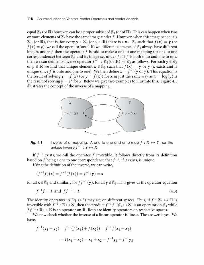
118 An Introduction to Vectors, Vector Operators and Vector Analysis
equal E3 (or R) however, can be a proper subset of E3 (or of R). This can happen when twoor more elements of E3 have the same image under f . However, when this image set equalsE3, (or R), that is, for every y ∈ E3 (or y ∈ R) there is a x ∈ E3 such that f (x) = y (orf (x) = y), we call the operator ‘onto’. If two different elements of E3 always have differentimages under f then the operator f is said to make a one to one mapping (or one to onecorrespondence) between E3 and its image set under f . If f is both onto and one to one,then we can define its inverse operator f −1 : E3(or R) 7→ E3 as follows. For each y ∈ E3or y ∈ R we find that unique element x ∈ E3 such that f (x) = y or y (x exists and isunique since f is onto and one to one). We then define x = f −1(y or y). This equation isthe result of solving y = f (x) (or y = f (x)) for x in just the same way as x = log(y) isthe result of solving y = ex for x. Below we give two examples to illustrate this. Figure 4.1illustrates the concept of the inverse of a mapping.
Fig. 4.1 Inverse of a mapping. A one to one and onto map f : X 7→ Y has theunique inverse f −1 : Y 7→ X
If f −1 exists, we call the operator f invertible. It follows directly from its definitionbased on f being a one to one correspondence that f −1, if it exists, is unique.
Using the definition of the inverse, we can write,
(f −1f )(x) = f −1(f (x)) = f −1(y) = x
for all x ∈ E3 and similarly for f f −1(y), for all y ∈ E3. This gives us the operator equation
f −1f = I and f f −1 = I . (4.3)
The identity operators in Eq. (4.3) may act on different spaces. Thus, if f : E3 7→ R isinvertible with f −1 : R 7→ E3 then the product f −1f : E3 7→ E3 is an operator on E3 whilef f −1 : R 7→R is an operator on R. Both are identity operators on respective spaces.
We now check whether the inverse of a linear operator is linear. The answer is yes. Wehave,
f −1(y1 + y2) = f −1(f (x1) + f (x2)) = f −1f (x1 + x2)
= I(x1 + x2) = x1 + x2 = f −1y1 + f−1y2
Linear Operators 119
and
f −1(αy) = f −1(αf (x)) = f −1f (αx) = αx = αf −1(y),
which proves the linearity of f −1.For any linear operator f we show that f (0) = 0. We have
f (0) = f (x− x) = f (x)− f (x) = 0.
For an invertible operator, f (a) = 0 implies a = 0 as can be seen from
0 = f −1(0) = f −1(f (a)) = a,
where the first equality follows because f −1 is a linear operator, so that f −1(0) = 0.Next we show that for an invertible operator f the set f (x),f (y),f (z) is linearly
independent (non-coplanar) provided the set x,y,z is linearly independent(non-coplanar). We see that the equation
0 = αf (x) + βf (y) + γf (z) = f (αx+ βy+ γz)
implies that all the coefficients α,β,γ vanish, because x,y,z are linearly independent.Here, we have used f (a) = 0 implies a = 0 for an invertible operator. The same argumentshows that if x,y,z are linearly dependent, then so are f (x),f (y),f (z).
For arbitrary x ∈ E3, let f gx = y, so that x = (f g)−1y. Successively multiplying bothsides by (f )−1 and (g)−1 we get x = (g)−1(f )−1y. This leads to the operator equality
(f g)−1 = (g)−1(f )−1.
4.1.3 Determinant of an invertible linear operator
Consider an orthonormal basis σ1, σ2, σ3 forming a right handed system. Theparallelepiped with adjacent sides σ1, σ2, σ3 is a cube with volume unity (unit cube). Thatis, σ1 · σ2 × σ3 = 1. Under the action of an invertible linear operator f : E3 7→ E3 thisunit cube goes over to a parallelepiped with adjacent sides f (σ1),f (σ2),f (σ3) and withvolume proportional to that of the unit cube σ1 · σ2 × σ3 = 1. We write
f (σ1) · f (σ2)× f (σ3) = det f σ1 · σ2 × σ3 = det f .
This equation defines the proportionality factor det f which depends exclusively on theoperator f and is an important characteristic of f . det f is called the determinant of theoperator f . Note that for an invertible operator f , det f , 0 because the vectorsf (σ1),f (σ2),f (σ3) are linearly independent, that is non-coplanar. Given any set x,y,zof linearly independent (non-coplanar) vectors, the number of unit cubes that can beaccommodated in the parallelepiped with adjacent sides x,y,z is given by its volume
120 An Introduction to Vectors, Vector Operators and Vector Analysis
x · y× z. Under the action of f , a unit cube is transformed to a parallelepiped with volumedet f . Therefore, the volume of the parallelepiped transformed under the action of f is
f (x) · f (y)× f (z) = det f x · y× z,
or,
det f =f (x) · f (y)× f (z)
x · y× z. (4.4)
The determinant det f of an invertible linear operator is invariant under the change oforthonormal basis. We shall see later that any two triads of orthonormal unit vectors canbe made to coincide by three successive independent rotations called Euler rotations (seesection 6.5). Under these rotations the volume of the unit cube scanned by one orthonormaltriad does not change. Since the determinant of f is simply the volume of the deformedunit cube under the action of f , we see that det f is invariant under the change of basis,which amounts to the rotation of one orthonormal triad of vectors to the other.
If f is invertible, then we know that any non-coplanar triad (x,y,z) is mapped toanother non-coplanar triad (f (x),f (y),f (z)). This makes both the numerator and thedenominator on the RHS of Eq. (4.4) non-zero, that is, det f , 0. Thus, if f is invertible,then det f , 0.
If f is not invertible, then there exist two vectors x,y ∈ E3, x , y such that f (x) =f (y). We can make a linearly independent triad (x,y,z) by adding a non-coplanar vectorz to the set x,y, x , y satisfying f (x) = f (y). Using this triad in Eq. (4.4), we see thatdet f = 0. This proves that det f , 0 implies f is invertible.
The last two paragraphs together imply that a linear operator f is invertible if and onlyif det f , 0.
Many simple properties of the determinant det f now follow. First, it is trivial to checkthat det I = 1. Next, consider the product gf of two linear invertible operators g and f .We have, using an orthonormal basis σ1, σ2, σ3,
det gf = gf (σ1) · gf (σ2)× gf (σ3)
= g(f (σ1)) · g(f (σ2))× g(f (σ3))
=
(g(f (σ1)) · g(f (σ2))× g(f (σ3))
f (σ1) · f (σ2)× f (σ3)
)(f (σ1) · f (σ2)× f (σ3))
= det g ·det f .
Thus, the determinant of the product is the product of determinants. This result can beused to write
1 = det I = det f f −1 = (det f )(det f −1), or, det f −1 = (det f )−1.
Linear Operators 121
If det f < 0, the operator f not only scales the volume of the parallelepiped formed by(x,y,z) however, also changes its orientation. That is, f changes a right handed systemformed by (x,y,z) to a left handed one or the acute angle between x and y×z to an obtuseangle between them. (see the interpretation of the scalar triple product in subsection 1.8.1).Further, det f is defined via a scalar triple product, so that interchange of any two factorschanges its sign. This is not surprising, because interchanging any two of the three linearlyindependent vectors changes them from a right handed to a left handed system and vice-versa (see section 1.16).
4.1.4 Non-singular operators
An operator f with det f = 0 is called singular. If det f , 0 then f is called non-singular.We can now prove that the following three statements are equivalent. We have proved someparts of it in the last two sections however, it is worth putting everything at one place.
(a) f is non-singular.(b) f (x) = 0 implies x = 0.(c) f is invertible.
We first prove (a) ⇒ (b). Let σk, k = 1,2,3 be an orthonormal basis. Assume thatf (x) = 0 for some x , 0. This means
f (x) =∑k
xkf (σk) = 0.
Since x , 0, not all xks can be zero. Therefore, the above equation means that the vectorsf (σk) k = 1,2,3 are linearly dependent (coplanar). Therefore, det f = 0 whichcontradicts the assumption that f is non-singular.
(b)⇒ (c): Suppose that f is not invertible, that is, it is not a one to one correspondencebetween x and f (x) so that there are two different non-zero vectors x1 and x2 (x1 , x2)satisfying
f (x1) = y = f (x2),
which gives
0 = f (x1)− f (x2) = f (x1 − x2)
which means that there is a non-zero vector z = x1 − x2 with f (z) = 0. This contradictsassumption (b).
(c)⇒ (a) That f is invertible implies it is non-singular is proved in subsection 4.1.3.
4.1.5 Examples
We find the inverses of the following linear operators.
(a) f (x) = αx+ a(b · x).
122 An Introduction to Vectors, Vector Operators and Vector Analysis
(b) g(x) = αx+b× x.
(a) Let
y = f (x) = αx+ a(b · x). (4.5)
Dotting both sides with b we get,
y ·b = αx ·b+ (a ·b)(x ·b),
or,
x ·b =y ·b
α+ a ·b.
Multiply both sides by a to get
a(x ·b) =a(y ·b)α+ a ·b
.
Using Eq. (4.5) we get,
y−αx =a(y ·b)α+ a ·b
,
or,
x =yα−
a(y ·b)α(α+ a ·b)
= f −1(y).
(b)
y = g(x) = αx+b× x. (4.6)
Dot with b to get
b · y = αb · x. (4.7)
Cross with b to get
b× y = αb× x+b× (b× x). (4.8)
Using Eqs (4.6), (4.7) in Eq. (4.8) and identity I, we get,
b× y = α(y−αx) + (b · x)b− b2x
= αy− (α2 + b2)x+α−1(b · y)b,
Linear Operators 123
or,
x =αy+α−1(b · y)b− (b× y)
α2 + b2 = g−1(y).
Exercise In these two examples, check that f −1f (x) = x and f f −1(y) = y. Also,check whether both these operators are non-singular.
(c) We solve the vector equation
α1a1 +α2a2 +α3a3 = c (4.9)
for αis; ai, i = 1,2,3 and c being given, using vector methods. We then compareour solution with that obtained by Cramer’s rule for solving simultaneous equations.Cross the given equation with a3 to get
α1(a3 × a1) +α2(a3 × a2) = a3 × c
Dotting with a2 and solving for α1 we get
α1 =a2 · (a3 × c)
a2 · (a3 × a1).
Similarly,
α2 =a3 · (a1 × c)
a3 · (a1 × a2)
and
α3 =a1 · (a2 × c)
a1 · (a2 × a3).
The given vector equation is equivalent to
α1a11 +α2a12 +α3a13 = c1
α1a21 +α2a22 +α3a23 = c2
α1a31 +α2a32 +α3a33 = c3
where aij is the ith component of aj and ci is the ith component of c with respect to someorthonormal basis. By Cramer’s rule, its solution is

124 An Introduction to Vectors, Vector Operators and Vector Analysis
α1 =
∣∣∣∣∣∣∣∣∣c1 a12 a13
c2 a22 a23
c3 a32 a33
∣∣∣∣∣∣∣∣∣∣∣∣∣∣∣∣∣∣a11 a12 a13
a21 a22 a23
a31 a32 a33
∣∣∣∣∣∣∣∣∣,
where in the upper determinant the 1st column in [aij ] is replaced by [c1,c2,c3]T and
similarly for α2 and α3. It is straightforward to check that the two solutions are equivalent.If we try to apply the vector method given above to the equation with more than three
variables, (αi i = 1, . . . ,4 say), it fails. We can make one of the four terms vanish by takinga suitable cross product and treat the resulting equation in three unknowns by the methodgiven above. However, the vectors in the three term equation are all coplanar making thescalar triple product like a1 · (a2 × a3) vanish. Thus, a generalization of our method needsa more general kind of algebraic setting, than the vector compositions based on dot andcross products. Geometric algebra is such an algebra in which the above method can begeneralized. We refer to references [10, 7, 11] for a comprehensive treatment of geometricalgebra.
4.2 Frames and Reciprocal FramesIn this section we deal with the problem of expressing arbitrary vectors in terms of anon-orthonormal basis. Let ek, k = 1,2,3 be a basis in E3, not necessarily orthonormal.We call it a frame and associate a pseudoscalar e = e1 · (e2 × e3) with this frame.e > 0(< 0) means the frame is positively (negatively) oriented. For an orthonormal frame(basis) e = +1 or e = −1 depending on whether it is right or left handed. The reciprocalframe ek, k = 1,2,3 is determined by the set of equations
ek · ej = δkj ; j,k = 1,2,3,
where δkj = 1 if j = k and zero otherwise. To solve for ek we note that it is a vector normalto both the vectors ej j , k and its scalar product with ek must be +1. Such a vector isuniquely given by the vector product of ej j , k in the cyclic order of 123. Thus, theunique solution to these equations are given by
e1 =e2 × e3
e,
e2 =e3 × e1
e,
e3 =e1 × e2
e.
Linear Operators 125
Exercise Check that an orthonormal frame is reciprocal to itself.
Any vector a can be expressed as a linear combination
a = a1e1 + a2e2 + a
3e3 = akek , (4.10)
where the summation convention is used on the right. The coefficients ak are calledcontravarient components of vector a (with respect to frame ek). We note that theEq. (4.10) is the same as Eq. (4.9) with α1,2,3 replaced by a1,2,3 and a1,2,3 replaced bye1,2,3 and c replaced by a. Making these substitutions, we get the following solutions forEq. (4.10).
a1 =a · (e2 × e3)
e1 · (e2 × e3),
a2 =a · (e3 × e1)
e1 · (e2 × e3),
a3 =a · (e1 × e2)
e1 · (e2 × e3). (4.11)
Exercise Show that these solutions reduce to
ak = ek · a; k = 1,2,3.
(Remember that ek , k = 1,2,3 are not mutually orthogonal!)If we expand a vector a in terms of the ek basis, we get
a = a1e1 + a2e2 + a3e3 = akek ,
where the coefficients ak are called covariant components of vector a (with respect toframe ek).
Exercise Show that the contravariant components ak are given by
ak = ek · a.
Exercise Let i, j, k be an orthonormal basis and define a non-orthonormal frame by e1 =
i+3j, e2 = 4j and e3 = k. Find the corresponding reciprocal frame. Find the contravariantand covariant components of a = 7i + 2j + k with respect to these frames. Draw figuresto depict both the frames and the contravariant and covariant components of a.
Exercise Show that primitive bases of the Bravis lattice of a crystal and its reciprocallattice form reciprocal frames.
126 An Introduction to Vectors, Vector Operators and Vector Analysis
4.3 Symmetric and Skewsymmetric OperatorsWe have already defined the adjoint of a linear operator. We now define two importanttypes of linear operators, namely symmetric and skewsymmetric operators.
A linear operator S is said to be symmetric (or self adjoint) if S = S† that is, if it isequivalent to its adjoint. Similarly, a linear operator A is said to be skewsymmetric (orantisymmetric) if A † = −A . A very simple but important observation is the followingidentity. For any operator f we can write,
f =12
(f + f †
)+
12
(f − f †
)= f+ + f−.
Obviously, the first term (f+) is a symmetric operator, while the second (f−) is askewsymmetric operator. Thus, any operator can be written as the sum of a symmetricand a skewsymmetric operator.
We now show that any skewsymmetric operator A can be put in a canonical (orstandard) form
A x = x× (a×b), (4.12)
where (a×b) is a unique pseudo vector.We first check whether this operator is indeed a skewsymmetric operator. We have,
y · (x× (a×b)) = y · ((b · x)a− (a · x)b),
= (b · x)(a · y)− (a · x)(b · y)
= −x · (y× (a×b)), (4.13)
giving
A † = −A .
Here, we have used identity I.We note that it is enough to prove Eq. (4.12) for a standard basis σk, k = 1,2,3, for
then the result is generally true by the linearity of A . We know that the vectors A σk andA †σ j can be written as
ak =A σk =∑j
σ jAjk ,
where Ajk = σ j ·A σk and
A †σ j =∑k
σkAjk ,
Linear Operators 127
where we have used the definition of the adjoint of an operator. Now we choose
a×b =12
∑k
ak × σk
and consider
σ j × (a×b) =12
∑k
σ j × (ak × σk)
=12
∑k
[(σ j · σk
)ak − σk
(σ j · ak
)]=
12
∑k
[δjk (A σk)− σkAjk
]=
12
(A σ j −A †σ j
)=A σ j . (4.14)
Here, we have used identity I and the orthonormality of the σk basis. As an example,the magnetic force due to magnetic field on a charged particle is a skewsymmetric linearoperator on the particle velocity given by F =Bv =
qcv×B acting via the psuedovector B.3
ExampleWe find the adjoint as well as the symmetric and the skewsymmetric parts of the operator
f x = αx+ a(b · x) + x× (c×d). (4.15)
We find
f †x = αx+b(a · x) + (c×d)× x,
f+x = αx+12[a(b · x) +b(a · x)],
and
f−x =12[a(b · x)−b(a · x)] + x× (c×d)
=12
x× (a×b) + x× (c×d). (4.16)
where f+ and f− are the symmetric and skewsymmetric parts of f respectively.
3Since F and v are polar vectors, B has to be a pseudovector.
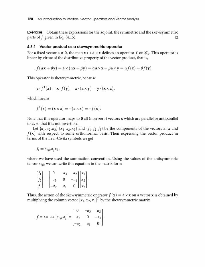
128 An Introduction to Vectors, Vector Operators and Vector Analysis
Exercise Obtain these expressions for the adjoint, the symmetric and the skewsymmetricparts of f given in Eq. (4.15).
4.3.1 Vector product as a skewsymmetric operator
For a fixed vector a , 0, the map x 7→ a× x defines an operator f on E3. This operator islinear by virtue of the distributive property of the vector product, that is,
f (αx+ βy) = a× (αx+ βy) = αa× x+ βa× y = αf (x) + βf (y).
This operator is skewsymmetric, because
y · f †(x) = x · f (y) = x · (a× y) = y · (x× a),
which means
f †(x) = (x× a) = −(a× x) = −f (x).
Note that this operator maps to 0 all (non-zero) vectors x which are parallel or antiparallelto a, so that it is not invertible.
Let a1,a2,a3 x1,x2,x3 and f1,f2,f3 be the components of the vectors a, x andf (x) with respect to some orthonormal basis. Then expressing the vector product interms of the Levi-Civita symbols we get
fi = εijkajxk ,
where we have used the summation convention. Using the values of the antisymmetrictensor εijk we can write this equation in the matrix form
f1f2f3
=
0 −a3 a2
a3 0 −a1
−a2 a1 0
x1
x2
x3
·Thus, the action of the skewsymmetric operator f (x) = a× x on a vector x is obtained bymultiplying the column vector [x1,x2,x3]
T by the skewsymmetric matrix
f ≡ a× ↔ [εijkaj ] ≡
0 −a3 a2
a3 0 −a1
−a2 a1 0
·
Linear Operators 129
4.4 Linear Operators and MatricesLet f be a linear operator and σk k = 1,2,3 be an orthonormal basis in E3. Using thefact that σk is a basis and the linearity of f , we can write
f (x) = f
∑k
(σk · x)σk
=∑k
(σk · x)f (σk),
where xk = σk ·x k = 1,2,3 are the components of x in the basis σk. We can expand thevectors fk = f (σk) in the basis σk to get
fk = f (σk) =∑j
σ j(σ j · fk) =∑j
σ jfjk .
There are three coefficients fjk for each value of k (that is, each fk) so that for k = 1,2,3there are nine coefficients fjk . We arrange them in a 3×3 matrix with j running over rowsand k over columns. We have,
[f ] = [fjk ] =
f11 f12 f13
f21 f22 f23
f31 f32 f33
·The coefficients
fjk = σ j · f (σk) = σ j · fk
which form a 3×3 matrix as above, are called the matrix elements of the linear operator f .The matrix formed by fjk is called the matrix representing f in the basis σk. If we changeover to some other orthonormal basis say ek, the matrix representing f in the basis ekis in general different than that representing f in the basis σk. Later in this discussion,we shall relate these two matrix representatives of the same operator f . By [f ]· we denotethe matrix representing operator f using the basis ·. Whenever the basis is fixed, we shalldrop the suffix ·.
A linear operator is completely determined by its matrix in a given basis. To see this,consider the action of f on an arbitrary vector x ∈ E3. We have,
f (x) =∑k
f (σk)xk =∑j
∑k
σ jfjkxk .
Thus, the vector f (x) has the following components along σ j .
(f (x))j =∑k
fjkxk .
130 An Introduction to Vectors, Vector Operators and Vector Analysis
Therefore, jth component of the vector equation
f (x) = y
is
(f (x))j =∑k
fjkxk = yj .
There is one such equation for each value of j = 1,2,3 so that the vector equation f (x) = yis equivalent to the set of three simultaneous equations∑
k
fjkxk = yj j = 1,2,3
completely determined by the matrix [fjk ]. Written in matrix form, these equations readf11 f12 f13
f21 f22 f23
f31 f32 f33
x1
x2
x3
=y1
y2
y3
·Thus, the action of a linear operator f on a vector x ∈ E3 is completely determined by thematrix of f in a given orthonormal basis. Note that the determinant of the matrix [fjk ]representing the linear operator f in the basis σk is the same as the determinant of f ,namely, det f = f (σ1) · f (σ2) × f (σ3) as can be seen by expressing this scalar tripleproduct in its determinant form (see the exercise in subsection 1.8.1). A student will dobetter by explicitly working out the matrix elements fjk for different values of the indicesj,k.
4.5 An Equivalence Between AlgebrasThe algebra of 3× 3 matrices is equivalent to the algebra of linear operators on E3. To seethis, we first note that the operator sum f + g corresponds to the matrix sum
(f + g)jk = σ j · (f (σk) + g(σk)) = σ j · f (σk) + σ j · g(σk) = fjk + gjk ,
where the first equality follows from the definition of the matrix element of an operator.Thus, the matrix element of the addition of two operators equals the addition of thematrix elements of the operators, or,
[f + g] = [f ] + [g].
For the product of two linear operators say gf consider (work this out),
Linear Operators 131
gf (σk) =∑j
(g(σ j))fjk =∑i
σ i
∑j
gijfjk
.
Compare with
gf (σk) =∑i
σ i(σ i · gf (σk))
to get∑j
gijfjk = σ i · gf (σk).
The RHS of this equation is the ikth element of the matrix of the operator gf , while theLHS is the ikth element of the product of the matrices of the operators g and f in thatorder. Thus, we see that
[gf ] = [g][f ]. (4.17)
The ikth element of the identity operator is,
σ i · I(σk) = σ i · σk = δik
because the basis σk is orthonormal. Thus, the matrix representing the identity operator,(which is the identity with respect to operator multiplication), is the unit matrix I , (whichis the identity with respect to matrix multiplication).
For an invertible operator f , using Eq. (4.17), we have,
I = [f −1f ] = [f −1][f ] (4.18)
which simply means that the matrix representing f −1 is the inverse of the matrixrepresenting f . Since f −1 is assumed to exist det f , 0. Since det f is the same as that ofthe matrix representing f , its determinant is non-zero and Eq. (4.18) is meaningful. Wehave already seen that det f is invariant under the change of orthonormal basis so thatEq. (4.18) holds irrespective of the orthonormal basis used. In fact we shall independentlyprove that the determinant of [f ] is invariant under the change of basis. In particular, thedeterminant of the operator f can be alternatively defined as the determinant of its matrixin any orthonormal basis.
Thus, we have shown that the set of linear operators on E3 and the set of matricesrepresenting them (with respect to a fixed orthonormal basis) are isomorphic under thebinary operations of addition and multiplication defined on these sets. This fact isexpressed by saying that the algebra of linear operators on E3 and that of their matrixrepresentatives are equivalent4.
4To establish this equivalence both sets must have the algebraic structure called ring with respect to the multiplications definedon them, which is known to be true. We shall not discuss this point any further.
132 An Introduction to Vectors, Vector Operators and Vector Analysis
We establish the relation between the matrix representing an operator and thatrepresenting its adjoint. We have,
f †jk = σ j · f †σk = f σ j · σk = σk · f σ j = fkj ,
which means
[f †] = [f ]T (4.19)
where the superscript T denotes the transpose of the matrix.
4.6 Change of BasisWe get the relation between the matrices of a linear operator f in two different orthonormalbases. We denote these bases by σk and ek. We write equation f (x) = y for basisσk as
FX = Y (4.20)
where F is the matrix of operator f in σk and X and Y are the column (3× 1) matricescomprising coordinates of vectors x and y in the basis σk (see the last equation insection 4.4). We write f (x) = y for the corresponding matrices in the basis ek as
F′X ′ = Y ′. (4.21)
It is straightforward to check, by expanding the basis ek using the basis σk, that for avector x ∈ E3,
X ′ = QX
with Qij = ei · σ j (4.22)
Apply Eq. (4.22) to X ′ and Y ′ in Eq. (4.21) to get
F′QX =QY
or,
(Q−1F′Q)X = Y (4.23)
Comparing Eq. (4.20) with Eq. (4.23) we have,
F =Q−1F′Q
F′ =QFQ−1
Linear Operators 133
The transformations induced by Q are called similarity transformations. Thus, thematrices of a linear operator in different bases are related by a similarity transformation,viaQ defined in Eq. (4.22).
It is now trivial to check that the determinant of a matrix of a linear operator f isinvariant under the change of basis. We have,
det(F′) = det(QFQ−1)
= det(Q)det(F)det(Q−1)
= det(QQ−1)det(F) = det(F).
Exercise Let g, f be linear operators on E3. Prove that
det[gf ] = det[g]det[f ]
and
det[f −1] = (det[f ])−1,
where det[·] is the determinant of the matrix representative of the corresponding operator.
5
Eigenvalues and Eigenvectors
5.1 Eigenvalues and Eigenvectors of a Linear OperatorSuppose a non-zero vector u is transformed into a scalar multiple of itself by a linearoperator f , that is,
f u = λu, (5.1)
where λ is a scalar. Then, we say that u is an eigenvector of f corresponding to theeigenvalue λ. Equation (5.1) is called the eigenvalue equation for the operatorf . Equation (5.1) remains valid if we multiply it by a non-zero scalar. Therefore, any scalarmultiple of u is also an eigenvector of f corresponding to the eigenvalue λ. However,these two eigenvectors are linearly dependent. If n ≥ 2 linearly independent1 eigenvectorscorrespond to the same eigenvalue, we call this eigenvalue n-fold degenerate. Thishappens when the eigenvalue equation is satisfied by n ≥ 2 linearly independenteigenvectors for the same eigenvalue. We will deal with the degenerate eigenvalues later.The problem of finding the eigenvalues and the corresponding eigenvectors of a givenlinear operator is called the eigenvalue problem for that operator. If we list out all thelinearly independent eigenvectors and the corresponding eigenvalues (if there is a m-folddegenerate eigenvalue, it will repeat m times in this list) it is called the spectrum of thecorresponding operator. This list of linearly independent eigenvectors obviously cannotexceed the dimension of the space on which the operator acts, as the number of linearlyindependent vectors cannot exceed the dimension. Thus, the maximum number oflinearly independent eigenvectors of a linear operator f acting on E3 is three.
If all the eigenvectors of an operator can form a basis of the space on which it acts, thatis, if the maximum number of linearly independent eigenvectors can be found, it is calleddiagonalizable. In our case the operator f on E3 is diagonalizable if all of the three linearlyindependent eigenvectors can be obtained. If all the eigenvalues of an operator are real and1That is, two non-collinear vectors, or three non-coplanar vectors. There cannot be more than three linearly independent
vectors in E3.
Eigenvalues and Eigenvectors 135
distinct (no degeneracy) then the operator can be proved to be diagonalizable. Even ifdegeneracy is present, we can find the maximal set of linearly independent eigenvectors,that is, the corresponding operator can be diagonalized. All the information of adiagonalizable operator is contained in its eigenvalues and eigenvectors because its actionon any vector, (by virtue of its linearity and by the fact that its eigenvectors form a basis),can be expressed in terms of these quantities in the simplest possible way. The differentialor integral equations, which are the principal mathematical models in physics andengineering, are often expressed or related to the eigenvalue problem of operators ondifferent kinds of spaces called function spaces. These are some of the reasons why theeigenvalue problem is of such a paramount importance in mathematical modeling of reallife processes. Here, we shall confine ourselves to the case of operators on E3 with realeigenvalues. As we shall see later, these are symmetric operators. We shall touch upon thecase of complex eigenvalues later.
The basis formed by the eigenvectors of an operator on E3 gives a coordinate frame inE3. Its coordinate axes are called principal axes and the frame is called the principal axessystem.
Typically, the operator is given in its matrix form [fjk ], that is, we are given the vectors
fk = f (σk) =3∑j=1
σ jfjk ,
where σ j is a suitable orthonormal basis.To develop a general method for solving the eigenvalue problem from this information,
we re-write the eigenvalue equation (Eq. (5.1)) as
(f −λI)u = 0. (5.2)
Equation (5.2) tells us that the operator (f −λI) must be singular because it maps a non-zero vector u , 0 to the zero vector, so that its determinant must vanish.
det (f −λI) = (f1 −λσ1) · [(f2 −λσ2)× (f3 −λσ3)] = 0. (5.3)
If we expand the LHS of Eq. (5.3), successively applying the distributive law for the scalarand the vector products, we can transform it to
λ3 −α1λ2 +α2λ−α3 = 0, (5.4)
where,
α1 =∑k
σk · fk = f11 + f22 + f33
α2 = σ1 · (f2 × f3) + σ2 · (f3 × f1) + σ3 · (f1 × f2)
α3 = det f = f1 · (f2 × f3) (5.5)
136 An Introduction to Vectors, Vector Operators and Vector Analysis
Exercise Establish Eqs (5.4) and (5.5).
Equation (5.3) or Eq. (5.4) are commonly called the secular equation for f . It is an algebraicequation of third degree in λ. From the fundamental theorem of algebra we know that athird degree polynomial has exactly three roots, or, has at most three distinct roots, a pair ofwhich could be complex. Even if you are a junior college student, you are expected to knowthis, may be without proof. These roots are the eigenvalues of f , because det(f −λI) = 0only when λ equals one of the roots or, the eigenvalue equation (Eq. (5.2)) is satisfied onlywhen λ equals one of the roots. We assume that this cubic polynomial in λ has three realroots, that is, all the eigenvalues of f are real. (That is, we assume the operator f to be asymmetric operator, to be defined in the next section).
Once the eigenvalues are known, the corresponding eigenvectors are found fromEq. (5.2). We expand u in Eq. (5.2) in terms of the basis σk and write Eq. (5.2) in theform
g1u1 + g2u2 + g3u3 = 0, (5.6)
where the vectors
gk = fk −λσk k = 1,2,3 (5.7)
are known for each eigenvalue λ and the scalar components uk = u · σk of the eigenvectorare to be determined2 for one eigenvalue λ. We can solve Eq. (5.6) for the ratios of uk asfollows. Cross Eq. (5.6) with g3 to get
(g3 × g1)u1 + (g3 × g2)u2 = 0. (5.8)
Dotting this with (g3 × g2)/|g3 × g2|2 we get
u2
u1=
(g3 × g1) · (g2 × g3)
|g3 × g1|2· (5.9)
Similarly,
u3
u1=
(g1 × g2) · (g2 × g3)
|g2 × g3|2· (5.10)
We have already seen that if u satisfies Eq. (5.2), so does any of its scalar multiples. Thismeans that the length or the sense (orientation) of u is not determined by the eigenvectorequation (Eq. (5.2)). Therefore, it is not a surprise that Eq. (5.6) fixes only the ratios of thecomponents of u and we are free to fix the sign and magnitude of u by assigning anyconvenient value to the component u1. After u1 is assigned a value, Eq. (5.9) andEq. (5.10) determine u2 and u3 uniquely. Here, we have assumed that every pair of vectors
2Note that the vectors (g1,g2,g3) must be coplanar, otherwise they form a linearly independent set of vectors and Eq. (5.6)has only the trivial solution ui = 0, i = 1,2,3.
Eigenvalues and Eigenvectors 137
formed out of (g1,g2,g3) is linearly independent, if not, all of them will be proportionalto each other3, in which case the ratios u2/u1 and u3/u1 obtained via Eq. (5.9) orEq. (5.10) will become indeterminate and Eqs (5.9), (5.10) do not apply. In such a case wecan proceed as follows. Since gks are proportional to each other, we can put g2 = cg1 andg3 = dg1 in Eq. (5.6) to get
(u1 + cu2 + du3)g1 = 0,
or, since g1 , 0,
u1 + cu2 + du3 = 0. (5.11)
Thus, we can give arbitrary values to any two of the components of u and the remainingcomponent is fixed via Eq. (5.11). We can choose two sets of ui values in such a way thatthe resulting eigenvectors (via Eq. (5.6) or Eq. (5.11)) are linearly independent. Settingu1 = u2 = 1 in Eq. (5.6) for example, gives,
g1 + g2 + u3g3 = 0. (5.12)
Alternatively, choose u1 = 1 and u3 = 0 so Eq. (5.6) reduces to
g1 + u2g2 = 0. (5.13)
To get the respective eigenvectors, we have to solve Eq. (5.12) for u3 and Eq. (5.13) for u2respectively, which is trivially done using known g1 ∝ g2 ∝ g3. These eigenvectors aretrivially seen to be linearly independent. Any eigenvector corresponding to a differentchoice of components will be a linear combination of these two eigenvectors. Thus,linearly dependent pairs of gks (so that they are mutually proportional) imply that theeigenvectors belonging to the corresponding eigenvalue span a 2-D space i.e., a plane. Thisis to be contrasted with the fact that when every pair of the gks is linearly independent, theeigenvectors belonging to the corresponding eigenvalue span a 1-D space.
It turns out that if λ is a simple root of the secular equation (for a symmetric linearoperator f ), then every two of the three vectors gk = fk − λσk are necessarily linearlyindependent. Thus, the eigenvectors belonging to a simple root λ span a 1-D space i.e.,a real line in E3. If λ is a double root, every pair of gks is linearly dependent so that theeigenvectors belonging to a double rootλ span a 2-D space, i.e., a plane inE3. Note that anytwo linearly independent (i.e., non-collinear) vectors in this plane can be the eigenvectors.
A multiple root of a secular equation is said to be k-fold degenerate if the root hasmultiplicity k. To an eigenvalue with multiplicity k there correspond exactly k linearlyindependent eigenvectors (in E3, provided f is symmetric).
Eigenvalues of a symmetric operator are real. To get a flavor of the complex eigenvalues,(i.e., complex roots of the secular equation) consider the skewsymmetric operator
f x = x× (σ1 × σ2)
3This is because (g1,g2,g3) have to satisfy Eq. (5.6) with one or more ui , 0.
138 An Introduction to Vectors, Vector Operators and Vector Analysis
where σk is some orthonormal basis. Operating on this basis we get
f (σ1) = σ1 × (σ1 × σ2) = −σ2 = −iσ1
f (σ2) = σ2 × (σ1 × σ2) = σ1 = −iσ2
f (σ3) = 0 = 0σ3 (5.14)
Exercise Show that the secular equation for f is
λ(λ2 + 1) = 0
The root λ = 0 corresponds to the eigenvector σ3 in Eq. (5.14). The eigenvalue equationsfor the eigenvalue −i the first two of Eq. (5.14). The last equalities in these equationsderive from the fact that multiplication of a vector in the complex plane by −i results inthe clockwise rotation of that vector through π/2. In general, multiplication by eiθ resultsin the counterclockwise rotation through θ. Thus, we see that complex eigenvalues resultin the rotation of the eigenvectors.
5.1.1 Examples
We obtain the eigenvalues and eigenvectors of the operator f represented by the matrix
[f ] =
4 −1 −1−1 4 −1−1 −1 4
in an orthonormal basis σ1, σ2, σ3.
Operating on the basis by f we get
f (σ1) = 4σ1 − σ2 − σ3 = f1
f (σ2) = −σ1 + 4σ2 − σ3 = f2
f (σ3) = −σ1 − σ2 + 4σ3 = f3 (5.15)
From these vectors we find
f1 × f2 = 15(σ1 × σ2) + 5(σ2 × σ3) + 5(σ3 × σ1)
f2 × f3 = 5(σ1 × σ2) + 15(σ2 × σ3) + 5(σ3 × σ1)
f3 × f1 = 5(σ1 × σ2) + 5(σ2 × σ3) + 15(σ3 × σ1) (5.16)
Eigenvalues and Eigenvectors 139
Using Eqs (5.15) and (5.16) we get the values of the coefficients in the secular equation,
α1 = 4+ 4+ 4 = 12
α2 = 15+ 15+ 15 = 45
α3 = f1 · (f2 × f3) = 50 (5.17)
Hence, the secular equation is
λ3 − 12λ2 + 45λ− 50 = 0
which can be factored into
(λ− 2)(λ− 5)2 = 0.
So the eigenvalues are 2 (simple) and 5 (doubly degenerate).To get the eigenvectors for λ = 2 we prepare the vectors gk defined in Eq. (5.7) using
Eq. (5.15). We have,
g1 = f1 − 2σ1 = 2σ1 − σ2 − σ3
g2 = f2 − 2σ2 = −σ1 + 2σ2 − σ3
g3 = f3 − 2σ3 = −σ1 − σ2 + 2σ3 (5.18)
From this we find
g1 × g2 = 3(σ1 × σ2 + σ2 × σ3 + σ3 × σ1) = g2 × g3 = g3 × g1
Using this in Eqs (5.9) and (5.10) with u1 = 1 we get u2 = u3 = 1. Hence,
u1 = σ1 + σ2 + σ3 (5.19)
is the eigenvector belonging to the eigenvalue 2.To get the eigenvectors corresponding to λ= 5, we evaluate gk = fk − 5σk to find
g1 = g2 = g3 = −(σ1 + σ2 + σ3)
Using this in Eq. (5.12) we find u3 = −2 when u1 = u2 = 1 so that
u2 = σ1 + σ2 − 2σ3 (5.20)
140 An Introduction to Vectors, Vector Operators and Vector Analysis
is an eigenvector for λ = 5. To get the other linearly independent eigenvector, we find,from Eq. (5.13), that u2 = −1 when u1 = 1 and u3 = 0. Hence,
u3 = σ1 − σ2 (5.21)
is the other eigenvector. Therefore, every vector in the plane defined by u2 and u3 is aneigenvector with eigenvalue λ= 5. (Operate by f on any linear combination of u2 and u3).
Although, our method to find the eigenvalues and eigenvectors is sufficiently general, itmay cost us more work than necessary in special cases. Often, an eigenvector is known inadvance. Then, the corresponding eigenvalue is easily obtained via
(f (u) ·u)/|u|2
instead of using the secular equation. More often than not, an eigenvector can be identifiedeasily from the symmetries in the given problem. Thus, perusal of Eq. (5.15) shows thatadding these three equations we get
f (σ1 + σ2 + σ3) = 2(σ1 + σ2 + σ3),
so we know that 2 is the eigenvalue corresponding to eigenvector u = σ1 + σ2 + σ3, inagreement with the result of the general method, obtained after a lot of effort. In order toget the other two eigenvectors u1 and u2 we use the fact that any two vectors in the (u1,u2)plane will do. As we shall see in the next section, (u1,u2) plane is perpendicular to u1. Sowe can write u2 = σ1 + σ2 + u3σ3 and choose u3 such that
u1 ·u2 = (σ1 + σ2 + σ3) · (σ1 + σ2 + u3σ3) = 2+ u3 = 0
This gives u3 = −2, so u2 = σ1 + σ2 − 2σ3 which coincides with Eq. (5.20). FromEq. (5.15) we now find f (u2) = 5u2 so the eigenvalue is 5. The vector u1 × u2 =−3(σ1 − σ2) is orthogonal to both u1 and u2 and is proportional to the eigenvector u3 inEq. (5.21).
Exercise Obtain the eigenvectors and eigenvalues of the operators represented by thefollowing matrices in an orthonormal basis.
(i) [f ] =
1 0 50 −2 05 0 1
·
(ii) [f ] =
7
√6 −
√3
√6 2 −5
√2
−√
3 −5√
2 −3
·
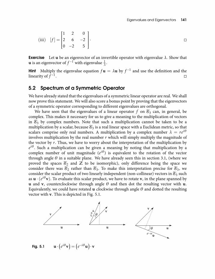
Eigenvalues and Eigenvectors 141
(iii) [f ] =
1 2 02 6 −20 −2 5
·
Exercise Let u be an eigenvector of an invertible operator with eigenvalue λ. Show thatu is an eigenvector of f −1 with eigenvalue 1
λ .
Hint Multiply the eigenvalue equation f u = λu by f −1 and use the definition and thelinearity of f −1.
5.2 Spectrum of a Symmetric OperatorWe have already stated that the eigenvalues of a symmetric linear operator are real. We shallnow prove this statement. We will also score a bonus point by proving that the eigenvectorsof a symmetric operator corresponding to different eigenvalues are orthogonal.
We have seen that the eigenvalues of a linear operator f on E3 can, in general, becomplex. This makes it necessary for us to give a meaning to the multiplication of vectorsin E3 by complex numbers. Note that such a multiplication cannot be taken to be amultiplication by a scalar, because E3 is a real linear space with a Euclidean metric, so thatscalars comprise only real numbers. A multiplication by a complex number λ = reiθ
involves multiplication by the real number r which will simply multiply the magnitude ofthe vector by r. Thus, we have to worry about the interpretation of the multiplication byeiθ. Such a multiplication can be given a meaning by noting that multiplication by acomplex number of unit magnitude (eiθ) is equivalent to the rotation of the vectorthrough angle θ in a suitable plane. We have already seen this in section 3.1, (where weproved the spaces E2 and Z to be isomorphic), only difference being the space weconsider there was E2 rather than E3. To make this interpretation precise for E3, weconsider the scalar product of two linearly independent (non-collinear) vectors in E3 suchas u · (eiθv). To evaluate this scalar product, we have to rotate v, in the plane spanned byu and v, counterclockwise through angle θ and then dot the resulting vector with u.Equivalently, we could have rotated u clockwise through angle θ and dotted the resultingvector with v. This is depicted in Fig. 5.1.
Fig. 5.1 u ·(eiθv
)=
(e−iθu
)· v
142 An Introduction to Vectors, Vector Operators and Vector Analysis
However, the alternative scalar product is just (e−iθu) · v. Thus, we have the general result
u · (λv) = (λ∗u) · v
where λ= reiθ is any complex number and λ∗ its complex conjugate.Now consider a symmetric linear operator S and its eigenvectors u and v belonging to
the eigenvalues λ1 and λ2 respectively, presumably complex. We have,
(λ1u) · v = S(u) · v = u · S(v) = u · (λ2v) = (λ∗2u) · v (5.22)
where we have used the fact that S is symmetric. Remember that when λ is complex, thevectors u and λu are not collinear. Equation (5.22) gives
(λ1 −λ∗2)u · v = 0. (5.23)
Two cases arise. In the first case, λ1 = λ2 = λ and the scalar product in Eq. (5.23) is non-zero. This gives λ = λ∗. This proves that the eigenvalues of a symmetric operator are real.In the second case, λ1 , λ2 so that the scalar product of the two eigenvectors u and v mustvanish. This simply means that the eigenvectors belonging to two different eigenvalues of asymmetric operator are orthogonal.
We now show that for every symmetric operator on E3, there exists a set of eigenvectorswhich are mutually orthogonal. The axes of the resulting frame are called the principalaxes. If all the three eigenvalues of the given symmetric operator are distinct, then thisstatement follows from the fact that the eigenvectors belonging to different eigenvalues of asymmetric operator must be orthogonal. Further, in this case, the eigenvectors are uniqueupto multiplication by a scalar (there is no degeneracy) so that all the principal axes areunique.
Now suppose λ1 , λ2, λ1 , λ3 but λ2 = λ3 = λ say. Since λ1 is distinct from λ2and λ3, the eigenvector u1 belonging to λ1 must be orthogonal to both the eigenvectorsbelonging to the degenerate eigenvalueλ. Further, we know that the eigenvectors belongingto λ are linearly independent (non-collinear) and every vector in the plane spanned by twolinearly independent eigenvectors for λ is also an eigenvector. Thus, we can take any vectorin the plane normal to u1 as one of the eigenvectors, say u2 of the eigenvalue λ and thethird eigenvector u3 can be obtained from
u3 = u1 ×u2.
If all the three eigenvalues are equal to say λ, three linearly independent eigenvectorsbelong to this common eigenvalue λ and every linear combination of them is also aneigenvector. In other words, every vector in E3 is an eigenvector belonging to λ.Obviously, any orthonormal triad of vectors (u1,u2,u3) gives a principal axes system.
The fact that a symmetric operator S has three orthogonal principal axes is expressedby the equations
Suk = λkuk k = 1,2,3
Eigenvalues and Eigenvectors 143
and
uj ·uk = 0 if j , k.
Thus, a symmetric operator is not only diagonalizable, but its eigenvectors naturally forman orthogonal basis.
Thus, we see that the eigenvectors of a symmetric operator form an orthogonal basisof E3. This basis is called the eigenbasis of the symmetric operator and the correspondingeigenvectors are called principal vectors and eigenvalues are called the principal values. Ifwe denote this basis by (u1,u2,u3) we can write an arbitrary vector x ∈ E3 as a linearcombination of the eigenvectors as
x = α1u1 +α2u2 +α3u3.
Dotting both sides by uk k = 1,2,3, using the orthogonality of the eigenvector basis anddividing both sides by |uk |2 we get
αk = (uk · x)/|uk |2.
Thus, the result of operating by a symmetric operator S on a vector x ∈ E3 can beexpressed as
Sx =3∑k=1
λkuk
[uk · x|uk |2
]=
3∑k=1
λkuk(uk · x) (5.24)
where uk is a unit vector in the direction of uk . Equation (5.24) is often written in terms ofthe so called projection operators. Thus,
Sx =
3∑k=1
λkPk
x,
where the projection operator Pk which projects any vector x ∈ E3 onto the kth principalaxis along uk is given by
Pkx = uk(uk · x). (5.25)
In terms of the projection operators, Eq. (5.24) can be re-expressed as
Sx =
∑k
λkPk
. (5.26)
The canonical form Eq. (5.24) or Eq. (5.26) is called the spectral decomposition (or thespectral form) of the symmetric operator S. Note that if we use an eigenvector uk in placeof x in the spectral decomposition, the eigenvalue equation for uk emerges trivially.
144 An Introduction to Vectors, Vector Operators and Vector Analysis
As we have already seen, an eigenvector multiplied by a scalar continues to be theeigenvector for the same eigenvalue. Thus, we can divide each of the eigenvectors by itsmagnitude to get the unit vector in its direction and this unit vector continues to be theeigenvector for the same eigenvalue. In this way, we can convert the orthogonal basiscomprising eigenvectors to the orthonormal basis comprising unit eigenvectors given byu1, u2, u3. We have used this orthonormal eigenbasis of the symmetric operator S whileobtaining Eqs (5.24), (5.26). We will always set up the matrix of a symmetric operator withrespect to its orthonormal eigenbasis.
Exercise Using its definition, establish the following properties of projection operators.
(a) Orthogonality: PjPk = 0 if j , k
(b) Idempotence: P 2k =Pk
(c) Completeness: P1 +P2 +P3 = I
Exercise Show that the matrix for a symmetric operator in its orthonormal eigenbasis isdiagonal, with its eigenvalues appearing on the diagonal.
Since the determinant of a diagonal matrix is the product of its diagonal elements, thedeterminant of a symmetric operator is the product of its eigenvalues. Thus, if one or moreof the eigenvalues of a symmetric operator are zero, its determinant is zero. Such asymmetric operator is singular, and hence non-invertible.
The matrix [S] representing a symmetric operator in an orthonormal basis σk k =1,2,3 is symmetric. We have, for the ijth element of such a matrix,
Sij = σ i · S(σ j) = S(σ i) · σ j = σ j · S(σ i) = Sji
where we have used the fact that S is symmetric. On the other hand, the matrix [A ]representing a skewsymmetric operatorA in an orthonormal basis is skewsymmetric. Wehave, for the ijth element of the matrix [A ],
Aij = σ i ·A (σ j) = −A (σ i) · σ j = −σ j ·A (σ i) = −Aji
where we have used the fact that A is skewsymmetric. Obviously, a matrix representinga skewsymmetric operator has vanishing diagonal elements because they have to satisfyAii = −Aii . That means, the pairs (σ i ,A σ i), i = 1,2,3 are orthogonal.
As you may have noticed, all the matrices given in the exercise at the end of the lastsection are symmetric.
From the spectral decomposition for a non-singular symmetric operator S, we canwrite, for the inverse operator,
S−1 =∑k
1λkPk . (5.27)
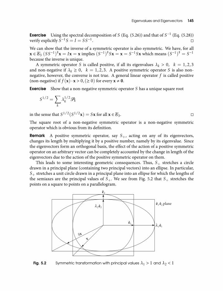
Eigenvalues and Eigenvectors 145
Exercise Using the spectral decomposition of S (Eq. (5.26)) and that of S−1 (Eq. (5.28))verify explicitly S−1S = I = SS−1.
We can show that the inverse of a symmetric operator is also symmetric. We have, for allx ∈ E3 (SS−1)†x = Ix = x implies (S−1)†Sx = x = S−1Sx which means (S−1)† = S−1
because the inverse is unique.A symmetric operator S is called positive, if all its eigenvalues λk > 0, k = 1,2,3
and non-negative if λk ≥ 0, k = 1,2,3. A positive symmetric operator S is also non-negative, however, the converse is not true. A general linear operator f is called positive(non-negative) if f (x) · x > 0, (≥ 0) for every x , 0.
Exercise Show that a non-negative symmetric operator S has a unique square root
S1/2 =∑k
λ1/2k Pk
in the sense that S1/2(S1/2x) = Sx for all x ∈ E3.
The square root of a non-negative symmetric operator is a non-negative symmetricoperator which is obvious from its definition.
Remark A positive symmetric operator, say S+, acting on any of its eigenvectors,changes its length by multiplying it by a positive number, namely by its eigenvalue. Sincethe eigenvectors form an orthogonal basis, the effect of the action of a positive symmetricoperator on an arbitrary vector can be completely accounted by the change in length of theeigenvectors due to the action of the positive symmetric operator on them.
This leads to some interesting geometric consequences. Thus, S+ stretches a circledrawn in a principal plane (containing two principal vectors) into an ellipse. In particular,S+ stretches a unit circle drawn in a principal plane into an ellipse for which the lengths ofthe semiaxes are the principal values of S+. We see from Fig. 5.2 that S+ stretches thepoints on a square to points on a parallelogram.
Fig. 5.2 Symmetric transformation with principal values λ1 > 1 and λ2 < 1
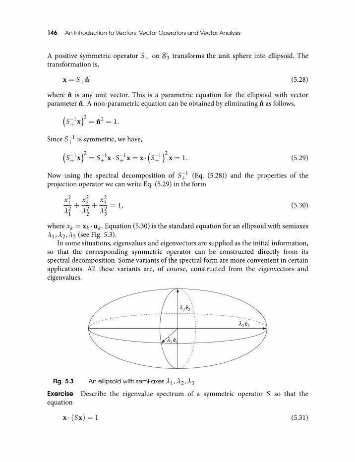
146 An Introduction to Vectors, Vector Operators and Vector Analysis
A positive symmetric operator S+ on E3 transforms the unit sphere into ellipsoid. Thetransformation is,
x = S+n (5.28)
where n is any unit vector. This is a parametric equation for the ellipsoid with vectorparameter n. A non-parametric equation can be obtained by eliminating n as follows.(
S−1+ x
)2= n2 = 1.
Since S−1+ is symmetric, we have,(S−1+ x
)2= S−1
+ x · S−1+ x = x ·
(S−1+
)2x = 1. (5.29)
Now using the spectral decomposition of S−1+ (Eq. (5.28)) and the properties of the
projection operator we can write Eq. (5.29) in the form
x21
λ21
+x2
2
λ22
+x2
3
λ23
= 1, (5.30)
where xk = xk ·uk . Equation (5.30) is the standard equation for an ellipsoid with semiaxesλ1,λ2,λ3 (see Fig. 5.3).
In some situations, eigenvalues and eigenvectors are supplied as the initial information,so that the corresponding symmetric operator can be constructed directly from itsspectral decomposition. Some variants of the spectral form are more convenient in certainapplications. All these variants are, of course, constructed from the eigenvectors andeigenvalues.
Fig. 5.3 An ellipsoid with semi-axes λ1,λ2,λ3
Exercise Describe the eigenvalue spectrum of a symmetric operator S so that theequation
x · (Sx) = 1 (5.31)
Eigenvalues and Eigenvectors 147
is equivalent to the standard coordinate forms for each of the following quadratic surfaces.
(a) Ellipsoid:
x21
a2 +x2
2
b2 +x2
3
c2 = 1,
(b) Hyperboloid of one sheet:
x21
a2 +x2
2
b2 −x2
3
c2 = 1,
(c) Hyperboloid of two sheets:
x21
a2 −x2
2
b2 −x2
3
c2 = 1.
Answer (a) All positive, (b) One negative, (c) Two negative eigenvalues.
Exercise Obtain the solution set x of the equation
[f (x− a)]2 = 1
where f is any linear operator.
Solution The given equation is
f (x− a) · f (x− a) = 1
or,
(x− a) · f †f (x− a) = 1.
f †f is obviously a symmetric operator. Call it S. Therefore, the above equation becomes,
(x− a) · S(x− a) = 1. (5.32)
We know from the previous exercise that Eq. (5.32) corresponds to that for an ellipsoid ifall the eigenvalues of S are positive, hyperboloid of one sheet if one eigenvalue is negativeand hyperboloid of two sheets if two of the eigenvalues are negative. Obviously, there is nosolution for all negative eigenvalues of S. Note that, for Eq. (5.32), all the quadratic surfacesare centered at a.
5.3 Mohr’s AlgorithmWe have developed a general method of finding the spectrum of a linear operator acting onE3. Many a time we have to deal with the problem of finding the spectrum of a (typicallysymmetric) operator acting on a plane, which is a 2-D subspace of E3. Another situation
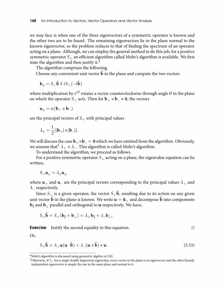
148 An Introduction to Vectors, Vector Operators and Vector Analysis
we may face is when one of the three eigenvectors of a symmetric operator is known andthe other two are to be found. The remaining eigenvectors lie in the plane normal to theknown eigenvector, so the problem reduces to that of finding the spectrum of an operatoracting on a plane. Although, we can employ the general method to do this job, for a positivesymmetric operator S+ an efficient algorithm called Mohr’s algorithm is available. We firststate the algorithm and then justify it.4
The algorithm comprises the following.Choose any convenient unit vector b in the plane and compute the two vectors
b± = S+b∓ iS+(−ib)
where multiplication by eiθ rotates a vector counterclockwise through angle θ in the planeon which the operator S+ acts. Then for b+ ×b− , 0, the vectors
u± = α(b+ ±b−)
are the principal vectors of S+ with principal values
λ± =12(|b+| ± |b−|).
We will discuss the case b+×b− = 0 which we have omitted from the algorithm. Obviously,we assume that5 λ+ , λ−. This algorithm is called Mohr’s algorithm.
To understand the algorithm, we proceed as follows.For a positive symmetric operator S+ acting on a plane, the eigenvalue equation can be
written,
S+u± = λ±u±
where u+ and u− are the principal vectors corresponding to the principal values λ+ andλ− respectively.
Since S+ is a given operator, the vector S+b, resulting due to its action on any givenunit vector b in the plane is known. We write u = u+ and decompose b into componentsb‖ and b⊥ parallel and orthogonal to u respectively. We have,
S+b = S+(b‖+b⊥) = λ+b‖+λ−b⊥,
Exercise Justify the second equality in this equation.
Or,
S+b = λ+u(u · b) +λ−(u× b)×u. (5.33)
4Mohr’s algorithm is discussed using geometric algebra in [10].5Otherwise, if S+ has a single doubly degenerate eigenvalue, every vector in the plane is an eigenvector and the other linearly
independent eigenvector is simply the one in the same plane and normal to it.
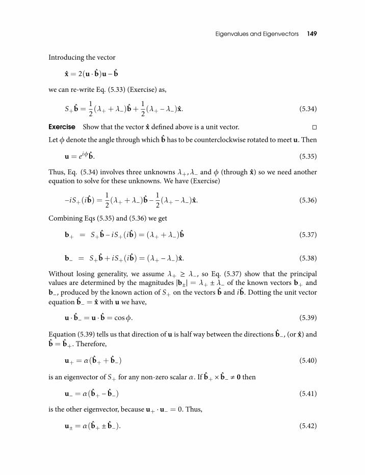
Eigenvalues and Eigenvectors 149
Introducing the vector
x = 2(u · b)u− b
we can re-write Eq. (5.33) (Exercise) as,
S+b =12(λ+ +λ−)b+
12(λ+ −λ−)x. (5.34)
Exercise Show that the vector x defined above is a unit vector.
Letφ denote the angle through which b has to be counterclockwise rotated to meet u. Then
u = eiφb. (5.35)
Thus, Eq. (5.34) involves three unknowns λ+,λ− and φ (through x) so we need anotherequation to solve for these unknowns. We have (Exercise)
−iS+(ib) =12(λ+ +λ−)b−
12(λ+ −λ−)x. (5.36)
Combining Eqs (5.35) and (5.36) we get
b+ = S+b− iS+(ib) = (λ+ +λ−)b (5.37)
b− = S+b+ iS+(ib) = (λ+ −λ−)x. (5.38)
Without losing generality, we assume λ+ ≥ λ−, so Eq. (5.37) show that the principalvalues are determined by the magnitudes |b±| = λ+ ± λ− of the known vectors b+ andb−, produced by the known action of S+ on the vectors b and ib. Dotting the unit vectorequation b− = x with u we have,
u · b− = u · b = cosφ. (5.39)
Equation (5.39) tells us that direction of u is half way between the directions b−, (or x) andb = b+. Therefore,
u+ = α(b+ + b−) (5.40)
is an eigenvector of S+ for any non-zero scalar α. If b+ × b− , 0 then
u− = α(b+ − b−) (5.41)
is the other eigenvector, because u+ ·u− = 0. Thus,
u± = α(b+ ± b−). (5.42)
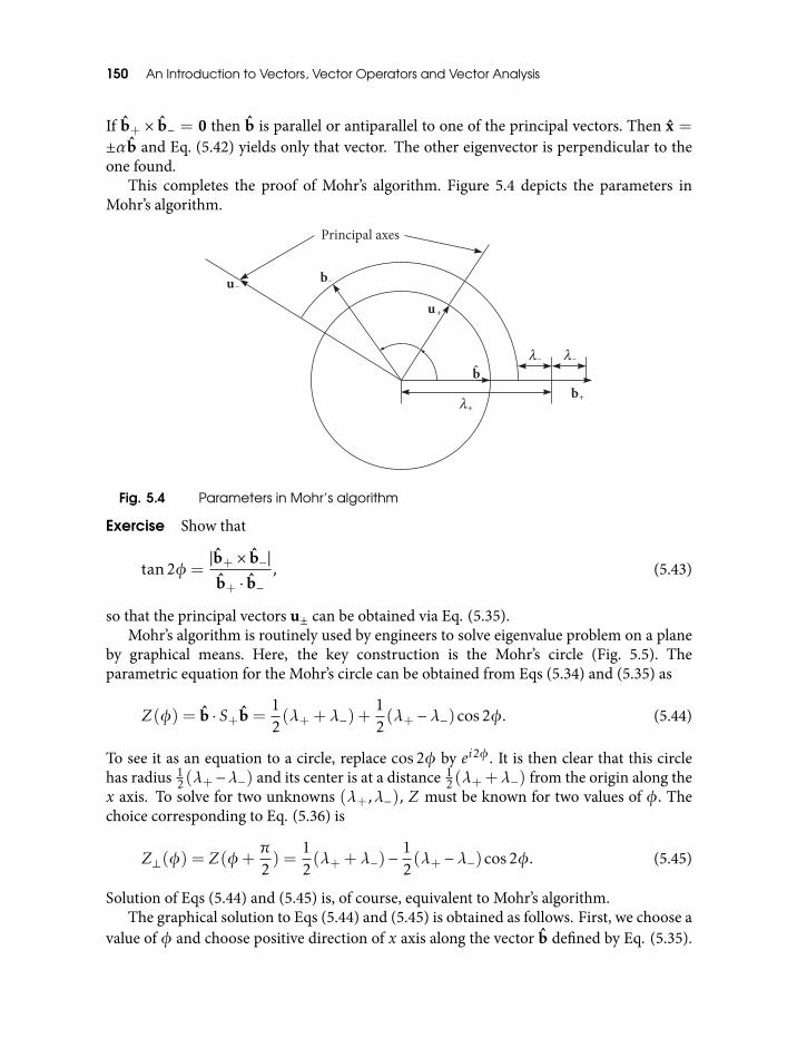
150 An Introduction to Vectors, Vector Operators and Vector Analysis
If b+ × b− = 0 then b is parallel or antiparallel to one of the principal vectors. Then x =±αb and Eq. (5.42) yields only that vector. The other eigenvector is perpendicular to theone found.
This completes the proof of Mohr’s algorithm. Figure 5.4 depicts the parameters inMohr’s algorithm.
Fig. 5.4 Parameters in Mohr’s algorithm
Exercise Show that
tan2φ =|b+ × b−|b+ · b−
, (5.43)
so that the principal vectors u± can be obtained via Eq. (5.35).Mohr’s algorithm is routinely used by engineers to solve eigenvalue problem on a plane
by graphical means. Here, the key construction is the Mohr’s circle (Fig. 5.5). Theparametric equation for the Mohr’s circle can be obtained from Eqs (5.34) and (5.35) as
Z(φ) = b · S+b =12(λ+ +λ−) +
12(λ+ −λ−)cos2φ. (5.44)
To see it as an equation to a circle, replace cos2φ by ei2φ. It is then clear that this circlehas radius 1
2(λ+−λ−) and its center is at a distance 12(λ++λ−) from the origin along the
x axis. To solve for two unknowns (λ+,λ−), Z must be known for two values of φ. Thechoice corresponding to Eq. (5.36) is
Z⊥(φ) = Z(φ+π2) =
12(λ+ +λ−)−
12(λ+ −λ−)cos2φ. (5.45)
Solution of Eqs (5.44) and (5.45) is, of course, equivalent to Mohr’s algorithm.The graphical solution to Eqs (5.44) and (5.45) is obtained as follows. First, we choose a
value of φ and choose positive direction of x axis along the vector b defined by Eq. (5.35).
Eigenvalues and Eigenvectors 151
This fixes b. Knowing the action of S+ on b, we can find the value of Z(φ) = b · S+b.We can calculate the value of Z⊥(φ) = Z(φ + π
2 ) in the same way, by noting that thecorresponding b vector is orthogonal to the x axis. Now, we draw a straight line making anangle 2φ with the positive direction of x axis, intersecting it at a point O. Then, we markout two points S1 and S2 on this line, which are equidistant from O and are at distancesZ(φ) and Z⊥(φ) from the origin respectively. While doing this, we may have to slide thisline parallel to itself along the x axis. Finally, we draw a circle (Mohr’s circle) with its centerat O and radius OS1,2. This circle cuts the x axis at two points at distance λ− (closer)and λ+ (farther) from the origin, giving us the required eigenvalues. All this is depictedin Fig. 5.5. One eigenvector is along the bisector of the angle 2φ made with the positivedirection of x axis and the second eigenvector is orthogonal to it.
Fig. 5.5 Mohr’s Circle
Exercise Where exactly would Mohr’s algorithm fail if the operator S+ was not positive?
5.3.1 Examples
(a) Using Mohr’s algorithm, we solve the eigenvalue problem for the operator
S+(b) = (a×b)× a+ (c×b)× c, (5.46)
where a and c are not collinear.
Exercise Show that S+(b) in Eq. (5.46) is both symmetric and positive.
The operator in Eq. (5.46) is the general form of the moment of inertia operator of aplane lamina. Note that
S+a = (c× a)× c = c2a− (a · c)c, (5.47)
where we have used identity I involving vector triple product and
−iS+(ia) = a2a+ (c · a)c. (5.48)
To understand Eq. (5.48), make use of Fig. 5.6 and construct the vector
−iS+(ia) = −i[(a× ia)× a+ (c× ia)× c] (5.49)
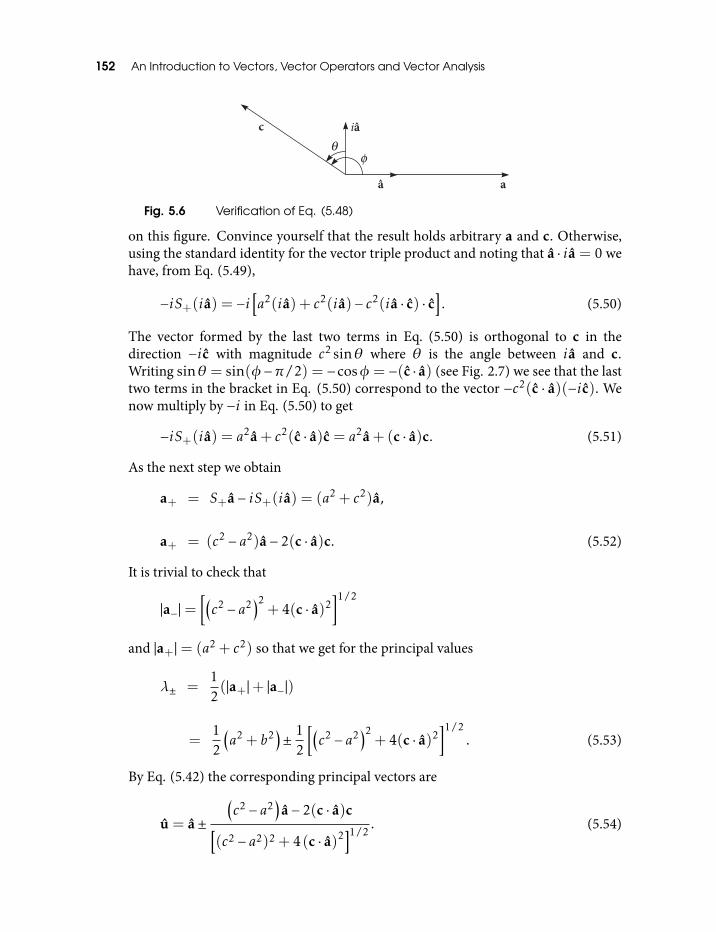
152 An Introduction to Vectors, Vector Operators and Vector Analysis
Fig. 5.6 Verification of Eq. (5.48)
on this figure. Convince yourself that the result holds arbitrary a and c. Otherwise,using the standard identity for the vector triple product and noting that a · ia = 0 wehave, from Eq. (5.49),
−iS+(ia) = −i[a2(ia) + c2(ia)− c2(ia · c) · c
]. (5.50)
The vector formed by the last two terms in Eq. (5.50) is orthogonal to c in thedirection −ic with magnitude c2 sinθ where θ is the angle between ia and c.Writing sinθ = sin(φ−π/2) = −cosφ = −(c · a) (see Fig. 2.7) we see that the lasttwo terms in the bracket in Eq. (5.50) correspond to the vector −c2(c · a)(−ic). Wenow multiply by −i in Eq. (5.50) to get
−iS+(ia) = a2a+ c2(c · a)c = a2a+ (c · a)c. (5.51)
As the next step we obtain
a+ = S+a− iS+(ia) = (a2 + c2)a,
a+ = (c2 − a2)a− 2(c · a)c. (5.52)
It is trivial to check that
|a−|=[(c2 − a2
)2+ 4(c · a)2
]1/2
and |a+|= (a2 + c2) so that we get for the principal values
λ± =12(|a+|+ |a−|)
=12
(a2 + b2
)± 1
2
[(c2 − a2
)2+ 4(c · a)2
]1/2. (5.53)
By Eq. (5.42) the corresponding principal vectors are
u = a±
(c2 − a2
)a− 2(c · a)c[
(c2 − a2)2 + 4 (c · a)2]1/2
. (5.54)
Eigenvalues and Eigenvectors 153
We note that a free choice of the argument b in Mohr’s algorithm enabled us tosimplify the computation by taking the special structure of the operator S+ intoaccount.
(b) We find the eigenvalues and eigenvectors of the operator
S+(b) = a(a ·b) + c(c ·b).
Exercise Show that S+(b) is symmetric as well as positive.
As in the previous example, we evaluate S+ at the defining unit vector a. We have,
S+a = a2a+ (c · a)
and
−iS+(ia) = −i(c · ia).
These can be written, by resolving c along a and ia as
S+a = a2a+ (·a)2a+ (c · a)(c · ia)ia,
−iS+(ia) = (c · ia)2a+ (c · a)(c · ia)ia.
This gives
a+ = S+a− iS+(ia) = (1+ a2)a+ 2(c · a)(c · ia)ia
a− = S+a+ iS+(ia) = [a2 + (c · a)2 − (c · ia)2]a (5.55)
or,
|a−| = a2 + (c · a)2 − |c× a|2
|a+| = [(1+ a2)2 + 4(c · a)2|c× a|2]1/2. (5.56)
Therefore,
λ± =12(|a+|+ |a−|)
=12
[(1+ a2
)2+ 4 (c · a)2 |c× a|2
]1/2
± 12
[a2 + (c · a)2 − |c× a|2
]. (5.57)
154 An Introduction to Vectors, Vector Operators and Vector Analysis
Exercise Show that an eigenvector u of S+ is obtained by rotating acounterclockwise by an angle φ satisfying
tan2φ =
(c2
1+ a2
)sin2θ
where θ is the angle between a and c.
(c) We find the eigenvalues and the eigenvectors of the operator
S+(e) = (a× e)× a+ (b× e)×b+ (c× e)× c, (5.58)
where
a+b+ c = 0.
Note that the condition a+b+c = 0 makes the vectors a,b,c coplanar and the givenoperator then acts on the plane containing a,b,c.
Exercise Show that S+ in Eq. (5.58) is both, symmetric and positive.
Hint Use identity I.
Thus, Mohr’s algorithm applies. We proceed on the same line as the previousexamples. We get,
S+(a) = (b2 + c2)a− (a ·b)b− (a · c)c (5.59)
−iS+(ia) = a2a+ (a ·b)b+ (a · c)c. (5.60)
This gives,
a+ = S+(a)− iS+(ia) = (a2 + b2 + c2)a, (5.61)
a− = S+(a)− iS+(ia) = (b2 + c2 − a2)a− 2(a ·b)b− 2(a · c)c. (5.62)
We now make use of the condition a+b+ c = 0 and simplify Eq. (5.61) to
a+ = 2(a2 + b2 + a ·b)a (5.63)
a− = 2(b2 − a2)a− 4(a ·b)b. (5.64)
We have,
|a−|= 2[(b2 − a2)2 + 4(a ·b)2]1/2.
Eigenvalues and Eigenvectors 155
Therefore, the principal values are
λ± =12(|a+| ± |a−|) = (a2 + b2 + a ·b)± [(b2 − a2)2 + 4(a ·b)2]1/2
and the corresponding eigenvectors are
u± = a±(b2 − a2)a− 2(a ·b)b
[(b2 − a2)2 + 4(a ·b)2]1/2.
Exercise Find the eigenvalues and the eigenvectors of the positive symmetricoperator
S+(b) = a(c ·b) + c(a ·b).
Unfortunately, no generalization of Mohr’s algorithm to the eigenvalue problem of apositive symmetric operator acting on 3-D space is available. However, as mentionedbefore, knowledge of one eigenvector enables us to use Mohr’s algorithm to find theremaining two eigenvectors in the plane orthogonal to the known eigenvector. Forexample, any operator constructed out of two vectors a and c necessarily has a× c asan eigenvector. Thus, for the operator in Eq. (5.46) we find
S+(a× c) = (a2 + c2)(a× c).
5.4 Spectrum of a 2 × 2 Symmetric MatrixWe find the eigenvalues and the eigenvectors of an operator f acting on a plane, given by asymmetric matrix
[S] =
[S11 S12
S12 S22
],
with respect to an orthonormal basis (σ1, σ2).The roots of the characteristic polynomial of a 2× 2 matrix A is easily seen to be
λ± =12[T r(A)±
√(T r(A))2 − 4 det(A)]
where T r(A) and det(A) mean the trace and the determinant of A respectively. Thisimmediately gives, for the eigenvalues of the symmetric matrix [S] above,
λ± =12(S11 + S22)±
12[(S11 − S22)
2 + 4S212]
1/2.
156 An Introduction to Vectors, Vector Operators and Vector Analysis
To get the eigenvectors, we assume the plane to be the complex plane and identify theorthonormal basis (σ1, σ2) with (σ1, iσ1). In this basis, σ1 has coordinates (1,0) andσ2 = iσ1 has coordinates (0,1). Therefore,
S(σ1) =
[S11 S12
S12 S22
][10
]=
[S11
S12
]and
S(iσ1) = S(σ2) =
[S11 S12
S12 S22
][01
]=
[S12
S22
].
The vector −iS(iσ1) is obtained by rotating S(iσ1) clockwise through π/2. This willinterchange its coordinates so that
−iS(iσ1) =
[S22
S12
]and we get,
b+ = S(σ1)− iS(iσ1) =
[S11 + S22
2S12
],
and
b− = S(σ1) + iS(iσ1) =
[S11 − S22
0
]·
We immediately see that b− is in the direction of σ1. So the angle χ between σ1 and b+ is
tanχ =2S12
S11 + S22.
However, we have seen before that the eigenvector u bisects the angle between b+ and b−or σ1. Denoting the angle between u and σ1 to be φ, we get
tan(2φ) =2S12
S11 + S22.
5.5 Spectrum of Sn
We define Sn = S S S · · ·S (n times), where S S(x) = S(S(x)). Let S be a symmetricoperator on E3 with eigenvalues λk. We show that Sn is symmetric with eigenvalues λnkand Sn has the same eigenvectors as S.
Eigenvalues and Eigenvectors 157
We prove the first claim by induction on n. Assume that for n= l,
S l =∑k
(λk)lPk . (5.65)
is the spectral representation of S l given by the projection operators Pk defined byEq. (5.25). Consider,
S l+1 =
∑k
(λk)lPk
∑j
(λj)Pj
=
∑k,j
(λk)lλjPjPk =
∑k,j
(λk)lλjδjkPk
=∑k
(λk)l+1Pk , (5.66)
where we have used the propertyPjPk = δjkPk of the projection operators. Thus, we haveshown that if S l is a symmetric operator (because of its spectral representation in termsof projectors) with eigenvalues (λk)l then S l+1 is a symmetric operator with eigenvalues(λk)
l+1. However, we know that Eq. (5.65) is true for l = 1 which is simply the spectralrepresentation of the symmetric operator S. Therefore, by induction, Eq. (5.65) must betrue for any value l = n.
To show that Sn and S share the same set of eigenvectors, consider an eigenvector u ofS with eigenvalue λ. We have,
Sn(u) = Sn−1(Su) = Sn−1(λu) = Sn−2(λSu) = Sn−2(λ2u) = · · ·= λnu.
Thus, we see that if u is an eigenvector of a symmetric operator S with an eigenvalue λ thenit is the eigenvector of the operator Sn with the eigenvalue λn. Thus, all the eigenvalues ofSn are real (because λ are real) so that Sn is also symmetric. Note that this proof goesthrough even if S were not symmetric and admitted complex eigenvalues. Therefore, theresult that S and Sn have common set of eigenvectors and eigenvalues of Sn are given bythe nth power of the eigenvalues of S is valid for a general linear operator.
Exercise If a,b,c are mutually orthogonal and S is a symmetric operator show that thethree vectors a× S(a), b× S(b) and c× S(c) are coplanar.
Hint If a,b,c were the principal vectors of S then each of the products a×S(a) etc, vanish.Therefore, let uk denote the orthogonal principal vectors of S. We have to show
(a× S(a)) · [(b× S(b))× (c× S(c))] = 0.
This can be done by using the spectral representation of S and the expansion of a,b,c inthe eigenbasis uk of S.
6
Rotations and Reflections
6.1 Orthogonal Transformations: Rotations and ReflectionsIn this section, we try and understand an extremely important class of linear operatorscalled orthogonal operators. These operators are frequently called transformationsbecause they correspond to rotations or reflections of points in space, which can bephysical operations of rotating (about some axis) or reflecting (with respect to a point or aplane) a point particle or a system of particles. An orthogonal operator preserves thelength of a vector in E3 as well as the orthogonality of vectors, say those forming anorthogonal basis.
An operator f is said to be orthogonal if it satisfies
f (x) · f (y) = x · y (6.1)
for all vectors x,y ∈ E3.A fixed point of an operator is the vector satisfying f (x) = x, that is, the vector left
invariant under the action of f . We know that the origin (the zero vector) is a fixed point off by virtue of its linearity. However, for an orthogonal operator acting on E3, no non-zerovector x∗ , 0 can be a fixed point, because for such a vector x∗ the orthogonality condition
x∗ · f (y) = x∗ · y (6.2)
is satisfied only by the vectors y whose projection along x∗ equals that of f (y) along x∗
and not by all vectors in E3. All vectors y and f (y) satisfying Eq. (6.2) for any given x,correspond to points which lie on a plane normal to x, so that an orthogonal operatorrestricted to act on a plane will leave invariant all vectors on a line normal to this planewhich is a 2-D subspace of E3 and we call it E2. To see this in another way, consider anorthogonal operator f on a plane. It has one fixed point on the plane namely the originon the plane. As a subspace of E3, this plane can be translated parallel to itself so that theorigin traces a line normal to the plane, all points on which are invariant under the action
Rotations and Reflections 159
of this f . Thus, an orthogonal operator acting on E3 leaves only one vector, namely theorigin or the zero vector, invariant, while an orthogonal operator acting on a plane leavesinvariant all points on a line normal to this plane. If we club this observation with the factthat an orthogonal operator preserves the length of a vector as well as the angle betweenvectors we see that an orthogonal operator corresponds to rotation (either about a point oran axis) or reflection in the origin or in a plane as we shall see below.
We now prove different properties of an orthogonal operator.Equation (6.1) can be rewritten
f (x) · f (y) = x · f †f (y) = x · y
which implies (in order to be consistent with Eq. (6.1)) that
f † = f −1. (6.3)
Thus, an orthogonal operator is a non-singular operator for which the inverse equals itsadjoint. The same property holds for the matrix representing an orthogonal operator. Tosee this, consider the jkth element of the matrix for the operator f †f ,
(f †f )jk = σ j · f †f σk = f σ j · f σk = σ j · σk = δjk , (6.4)
which means
[f †f ] = [f †][f ] = I (6.5)
where I is the 3× 3 unit matrix, giving
[f †] = [f ]−1. (6.6)
Written explicitly in elemental form, Eq. (6.5) becomes∑i
f †jifik = δjk ,
or, ∑i
fijfik = δjk , (1 ≤ j ≤ k ≤ 3), (6.7)
where we have used [f †] = [f ]T (Eq. (4.19)). The matrix satisfying Eq. (6.7) consists ofcolumns which are mutually orthogonal and individually normalized. Such a matrix iscalled orthogonal. Thus, an orthogonal operator is represented by an orthogonal matrix.
Exercise Show that the inverse of an orthogonal operator (matrix) is an orthogonaloperator (matrix).
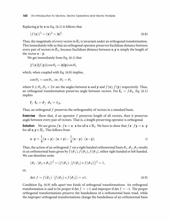
160 An Introduction to Vectors, Vector Operators and Vector Analysis
Replacing y by x in Eq. (6.1) it follows that
(f (x))2 = (x)2 = |x|2. (6.8)
Thus, the magnitude of every vector in E3 is invariant under an orthogonal transformation.This immediately tells us that an orthogonal operator preserves Euclidean distance betweenevery pair of vectors in E3, because Euclidean distance between x,y is simply the length ofthe vector x− y.
We get immediately from Eq. (6.1) that
|f (x)||f (y)|cosθ2 = |x||y|cosθ1
which, when coupled with Eq. (6.8) implies,
cosθ2 = cosθ1, or, θ2 = θ1
where 0 ≤ θ1,θ2 < 2π are the angles between x and y and f (x),f (y) respectively. Thus,an orthogonal transformation preserves angle between vectors. For fk = f σk , Eq. (6.1)implies
fj · fk = σ j · σk = δjk .
Thus, an orthogonal f preserves the orthogonality of vectors in a standard basis.
Exercise Show that, if an operator f preserves length of all vectors, then it preservesangle between every pair of vectors. That is, a length preserving operator is orthogonal.
Solution We are given f x · f x = x · x for all x ∈ E3. We have to show that f x · f y = x · yfor all x,y ∈ E3. This follows from
x · y =14(x+ y) · (x+ y)− 1
4(x− y) · (x− y).
Thus, the action of an orthogonal f on a right handed orthonormal basis σ1, σ2, σ3 resultsin an orthonormal basis given by f (σ1),f (σ2),f (σ3), either right handed or left handed.We can therefore write
(σ1 · [σ2 × σ3])2 = (f (σ1) · [f (σ2)× f (σ3)])
2 = 1,
or,
det f = f (σ1) · [f (σ2)× f (σ3)] = ±1. (6.9)
Condition Eq. (6.9) tells apart two kinds of orthogonal transformations. An orthogonaltransformation is said to be proper if det f = +1 and improper if det f = −1. The properorthogonal transformations preserve the handedness of a orthonormal basis triad, whilethe improper orthogonal transformations change the handedness of an orthonormal basis
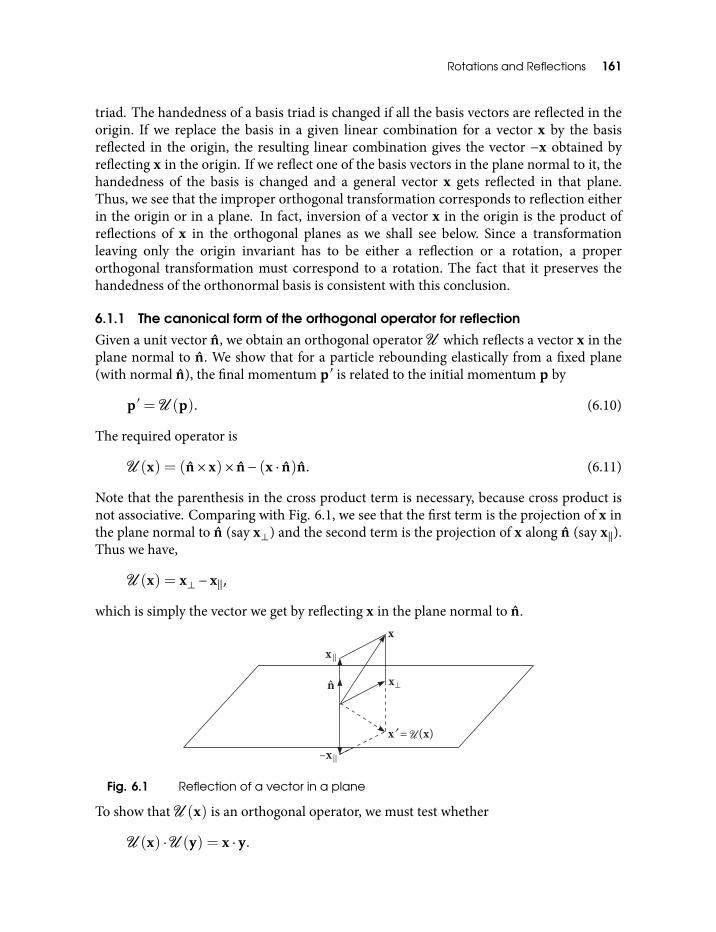
Rotations and Reflections 161
triad. The handedness of a basis triad is changed if all the basis vectors are reflected in theorigin. If we replace the basis in a given linear combination for a vector x by the basisreflected in the origin, the resulting linear combination gives the vector −x obtained byreflecting x in the origin. If we reflect one of the basis vectors in the plane normal to it, thehandedness of the basis is changed and a general vector x gets reflected in that plane.Thus, we see that the improper orthogonal transformation corresponds to reflection eitherin the origin or in a plane. In fact, inversion of a vector x in the origin is the product ofreflections of x in the orthogonal planes as we shall see below. Since a transformationleaving only the origin invariant has to be either a reflection or a rotation, a properorthogonal transformation must correspond to a rotation. The fact that it preserves thehandedness of the orthonormal basis is consistent with this conclusion.
6.1.1 The canonical form of the orthogonal operator for reflection
Given a unit vector n, we obtain an orthogonal operator U which reflects a vector x in theplane normal to n. We show that for a particle rebounding elastically from a fixed plane(with normal n), the final momentum p′ is related to the initial momentum p by
p′ = U (p). (6.10)
The required operator is
U (x) = (n× x)× n− (x · n)n. (6.11)
Note that the parenthesis in the cross product term is necessary, because cross product isnot associative. Comparing with Fig. 6.1, we see that the first term is the projection of x inthe plane normal to n (say x⊥) and the second term is the projection of x along n (say x‖).Thus we have,
U (x) = x⊥ − x‖,
which is simply the vector we get by reflecting x in the plane normal to n.
Fig. 6.1 Reflection of a vector in a plane
To show that U (x) is an orthogonal operator, we must test whether
U (x) ·U (y) = x · y.
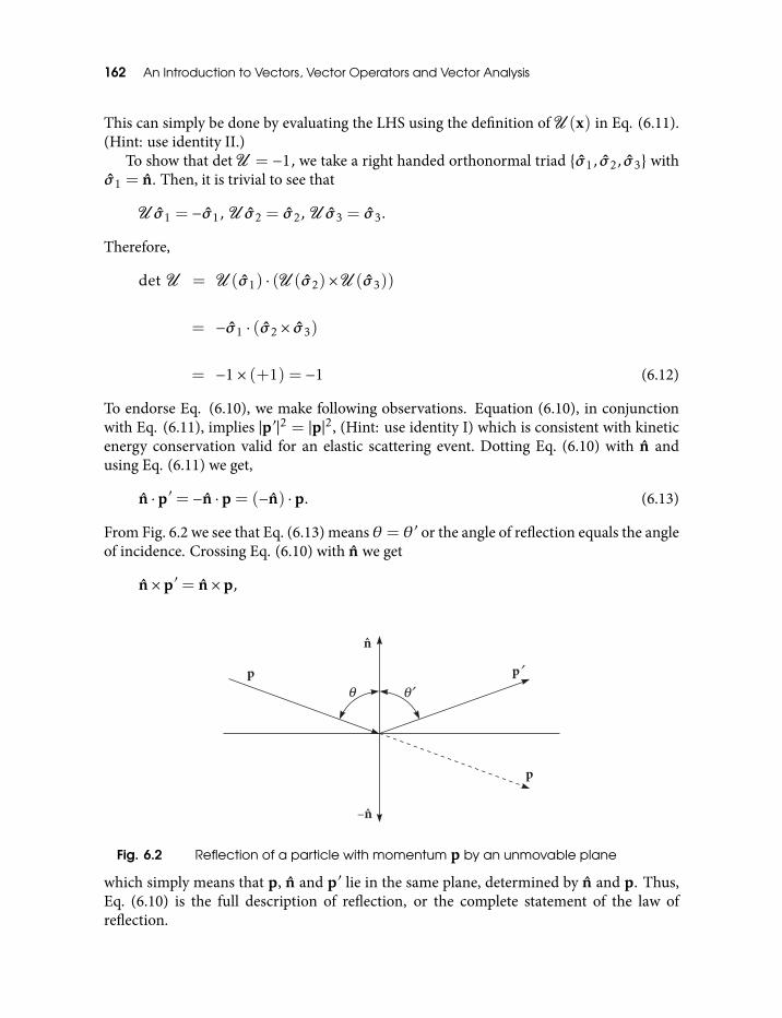
162 An Introduction to Vectors, Vector Operators and Vector Analysis
This can simply be done by evaluating the LHS using the definition of U (x) in Eq. (6.11).(Hint: use identity II.)
To show that det U = −1, we take a right handed orthonormal triad σ1, σ2, σ3 withσ1 = n. Then, it is trivial to see that
U σ1 = −σ1, U σ2 = σ2, U σ3 = σ3.
Therefore,
det U = U (σ1) · (U (σ2)×U (σ3))
= −σ1 · (σ2 × σ3)
= −1× (+1) = −1 (6.12)
To endorse Eq. (6.10), we make following observations. Equation (6.10), in conjunctionwith Eq. (6.11), implies |p′ |2 = |p|2, (Hint: use identity I) which is consistent with kineticenergy conservation valid for an elastic scattering event. Dotting Eq. (6.10) with n andusing Eq. (6.11) we get,
n ·p′ = −n ·p = (−n) ·p. (6.13)
From Fig. 6.2 we see that Eq. (6.13) means θ = θ′ or the angle of reflection equals the angleof incidence. Crossing Eq. (6.10) with n we get
n×p′ = n×p,
Fig. 6.2 Reflection of a particle with momentum p by an unmovable plane
which simply means that p, n and p′ lie in the same plane, determined by n and p. Thus,Eq. (6.10) is the full description of reflection, or the complete statement of the law ofreflection.
Rotations and Reflections 163
To find the inverse of U we note that y = U (x) implies x = U (y), that is, x andy are mutual images under reflection. (This establishes the operator equation U 2 = I .)Therefore, we have
U −1 = U . (6.14)
As a corollary, we can show that the reflection U is a symmetric operator. Orthogonalityof U coupled with Eq. (6.14) gives
U † = U −1 = U (6.15)
Exercise Prove that the product of three elementary reflections in orthogonal planes isan inversion, the linear transformation that reverses the direction of every vector.
Solution We denote by Un(x) the operator for reflection of x in the plane normal to n.Let σ1, σ2, σ3 be an orthonormal triad of vectors. Note that
Uσ j (σk) = −δjkσk + (1− δjk)σk (6.16)
Now let
x = σ1x1 + σ2x2 + σ3x3
be a vector in E3. We have, by virtue of Eq. (6.16),
Uσ3Uσ2Uσ1
(x) = −σ1x1 − σ2x2 − σ3x3 = −x (6.17)
which is what we wanted to prove.
If we successively reflect a vector in two different planes in different order, we get, ingeneral, two different vectors. This fact is expressed by saying that reflections, in general,do not commute. Thus, if U1, U2 denote the reflection operators for two planes then
U1U2(x) ,U2U1(x).
Exercise Show that the reflections defined via Eq. (6.16) commute.
Now consider two reflections which commute, that is, the corresponding reflectionoperators satisfy
U1U2(x) = U2U1(x)
for all x ∈ E3. Setting U = U1U2 we get
U † = (U1U2)† = U †2U
†1 = U2U1 = U1U2 = U
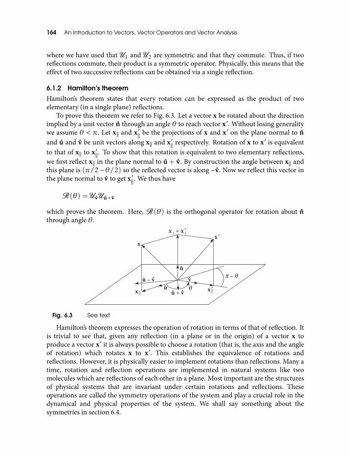
164 An Introduction to Vectors, Vector Operators and Vector Analysis
where we have used that U1 and U2 are symmetric and that they commute. Thus, if tworeflections commute, their product is a symmetric operator. Physically, this means that theeffect of two successive reflections can be obtained via a single reflection.
6.1.2 Hamilton’s theorem
Hamilton’s theorem states that every rotation can be expressed as the product of twoelementary (in a single plane) reflections.
To prove this theorem we refer to Fig. 6.3. Let a vector x be rotated about the directionimplied by a unit vector n through an angle θ to reach vector x′. Without losing generalitywe assume θ < π. Let x‖ and x′‖ be the projections of x and x′ on the plane normal to nand u and v be unit vectors along x‖ and x′‖ respectively. Rotation of x to x′ is equivalentto that of x‖ to x′‖. To show that this rotation is equivalent to two elementary reflections,we first reflect x‖ in the plane normal to u + v. By construction the angle between x‖ andthis plane is (π/2−θ/2) so the reflected vector is along −v. Now we reflect this vector inthe plane normal to v to get x′‖. We thus have
R(θ) = UvUu+v
which proves the theorem. Here, R(θ) is the orthogonal operator for rotation about nthrough angle θ.
Fig. 6.3 See text
Hamilton’s theorem expresses the operation of rotation in terms of that of reflection. Itis trivial to see that, given any reflection (in a plane or in the origin) of a vector x toproduce a vector x′ it is always possible to choose a rotation (that is, the axis and the angleof rotation) which rotates x to x′ . This establishes the equivalence of rotations andreflections. However, it is physically easier to implement rotations than reflections. Many atime, rotation and reflection operations are implemented in natural systems like twomolecules which are reflections of each other in a plane. Most important are the structuresof physical systems that are invariant under certain rotations and reflections. Theseoperations are called the symmetry operations of the system and play a crucial role in thedynamical and physical properties of the system. We shall say something about thesymmetries in section 6.4.
Rotations and Reflections 165
6.2 Canonical Form for Linear OperatorsOf all the linear operators, the symmetric, positive and orthogonal operators are the mostimportant in modeling the physical world. The symmetric operators are diagonalizable,have real eigenvalues and their eigenvectors can form an orthonormal basis of E3. Sincethe magnitudes of all vector quantities are real, only real eigenvalues can correspond to thevalues of any measurable physical quantity. Further, the action of a symmetric operator onan arbitrary vector can be obtained via its action on its eigenvectors. This is possible onlybecause a symmetric operator has real eigenvalues and its eigenvectors form a basis.A positive symmetric operator has positive eigenvalues having simple geometricinterpretation and are required to express many physical quantities that are positive, e.g.,the kinetic energy of a rotating rigid body expressed using the moment of inertia operator.Finally, orthogonal operators are required to incorporate elementary physical operationslike reflection and rotation of a system. All this motivates a question whether a givenlinear operator can be expressed in terms of these operators. If this is possible, the actionof such an operator on an arbitrary vector can be completely understood and carried out.In this section, we try and answer this question.
We start by proving that every symmetric transformation can be expressed asthe product of a symmetric orthogonal transformation and a positive symmetrictransformation. We proceed as follows.
Let S be a symmetric operator and let ek k = 1,2,3 be its eigenvectors forming anorthonormal frame. Define the reflections
Uej (ek) = −δjkek + (1− δjk)ek
as in Eq. (6.16). We know that Uej reverse the direction of ej and that their products areorthogonal and symmetric. Now consider the spectral representation of S ,
S =∑k
λkPk
and define a positive symmetric operator
S+ =∑k
|λk |Pk .
We consider four cases.
(i) All λk ≥ 0. We write
S = IS+.
(ii) One eigenvalue (say jth) < 0. (λj < 0). We write
S = UejS+.
166 An Introduction to Vectors, Vector Operators and Vector Analysis
(iii) Two eigenvalues (say ith and jth < 0. (λi < 0,λj < 0). We write
S = UeiUejS+.
(iv) All the eigenvalues < 0. We write
S = Ue1Ue2Ue3
S+.
There are no other cases and in each of the above case we have shown that the symmetricoperator S can be written as the product of a symmetric orthogonal operator and a positivesymmetric operator.
Next, we obtain a unique rotationR for an arbitrary improper orthogonal operatorIsatisfying
I =RU ,
where U is a simple reflection in the plane normal to any direction u as expressed by itscanonical form Eq. (6.11).
We use the fact that U 2 = I to write
I = (I U )U
and defineR = I U . The fact thatR is a rotation follows from
det R = (det I )(det U )
= (−1)(−1) = 1.
Next, we prove the Polar Decomposition Theorem which states that every non-singularoperator f has a unique decomposition in the form
f =RS = I R , (6.18)
whereR is a rotation and S and I are positive symmetric operators given by
S = (f †f )1/2
I = (f f †)1/2. (6.19)
A canonical form for f is therefore obtained from that forR and S.To prove Eq. (6.18) we note that
y · (f †f x) = f (y) · f (x) = x · (f †f y),
Rotations and Reflections 167
so that the operator S ′ defined by
S ′ = f †f
is symmetric. Further,
x · (f †f x) = (f x)2 > 0 if x , 0
which makes S ′ positive. Therefore, the square root of S ′ = f †f is well defined and unique
S = (f †f )1/2.
Since S is non-singular, we solve Eq. (6.18) for the rotationR ,
R = f −1 = f (f †f )−1/2. (6.20)
We have,
detf † = det f ,
or,
det(f †f ) = (det f )2,
or,
det S−1 = det(f †f )−1/2 = (det f )−1,
or,
det R = (det f )(det S−1) = 1,
which shows thatR is a rotation. The other part of Eq. (6.18) namely,
f = I R
is proved similarly.The eigenvalues and eigenvectors of S decide the basic structural properties of f (see
below for a geometric interpretation), because the other factor is just a rotation. They aresometimes called principal vectors and principal values of f to distinguish them fromeigenvectors and eigenvalues of f which may, in general, be complex and are not related ina simple way with the principal values which are always real. Of course, there is nodistinction if f itself is symmetric. Equation (6.18) clearly tells us that complexeigenvalues correspond to rotations as we have seen before (see section 5.2).
The polar decomposition, Eq. (6.18), provides a simple geometrical interpretation forany linear operator f . Consider the action of f on points x of a 3-D body or a geometrical

168 An Introduction to Vectors, Vector Operators and Vector Analysis
figure. According to Eq. (6.18), the body is first stretched and/or reflected along theprincipal directions of f . Then, the deformed body is rotated about the axis through theangle both specified byR .
6.2.1 Examples
(a) We find the polar decomposition of the skewsymmetric transformation
f (x) = x× (a×b). (6.21)
Using the skew symmetry of f (f † = −f ) we can write
f †f = (a×b)× (x× (a×b))
= (a×b)2x− [(a×b) · x](a×b) (6.22)
where we have used identity I. Note that
y · f †f x = (a×b)2x · y− [(a×b) · x][(a×b) · y]
= x · f †f y (6.23)
which means that f †f is a symmetric operator. Further, x·f †f x > 0 for x , 0 makingf †f a positive operator. It is easily verified that the square root operator is given by
S = (f †f )1/2 = |a×b|x− (a×b) · xa×b (6.24)
where a×b is the unit vector in the direction of a×b.We now find the rotation R in Eq. (6.18) with f given by Eq. (6.21). We have
already found S. We note that (a×b) · S(x) = 0 so that Sx lies in the plane normalto a×b. Thus, we need to rotate Sx about a×b through π/2, soR =Ra×b(π/2).Taking this plane to be the complex plane, and real and imaginary axes along Sx andf x respectively, this rotation amounts to multiplication by eiπ/2 = i.1
(b) The linear transformation
f x = x+ 2ασ1(σ2 · x) (6.25)
is called a shear. Figure 6.4 shows the effect of f on a unit square in the σ1σ2 plane.We find the eigenvectors, eigenvalues, principal vectors and principal values of f inthis plane. We also find the angle of rotation in the polar decomposition of f .
It is easily seen that the only eigenvector of f in Eq. (6.25) is σ1 satisfying
f (σ1) = σ1 (6.26)1Note that f (x) is perpendicular to both, a×b and S(x).
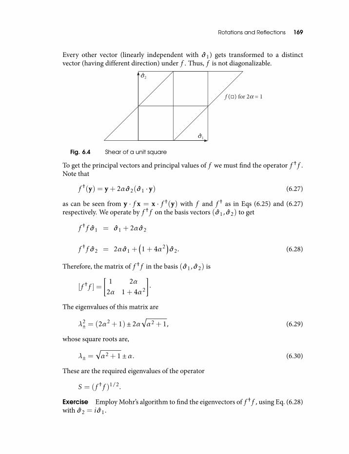
Rotations and Reflections 169
Every other vector (linearly independent with σ1) gets transformed to a distinctvector (having different direction) under f . Thus, f is not diagonalizable.
Fig. 6.4 Shear of a unit square
To get the principal vectors and principal values of f we must find the operator f †f .Note that
f †(y) = y+ 2ασ2(σ1 · y) (6.27)
as can be seen from y · f x = x · f †(y) with f and f † as in Eqs (6.25) and (6.27)respectively. We operate by f †f on the basis vectors (σ1, σ2) to get
f †f σ1 = σ1 + 2ασ2
f †f σ2 = 2ασ1 +(1+ 4α2
)σ2. (6.28)
Therefore, the matrix of f †f in the basis (σ1, σ2) is
[f †f ] =
[1 2α
2α 1+ 4α2
]·
The eigenvalues of this matrix are
λ2± = (2α2 + 1)± 2α
√α2 + 1, (6.29)
whose square roots are,
λ± =√α2 + 1±α. (6.30)
These are the required eigenvalues of the operator
S = (f †f )1/2.
Exercise Employ Mohr’s algorithm to find the eigenvectors of f †f , using Eq. (6.28)with σ2 = iσ1.
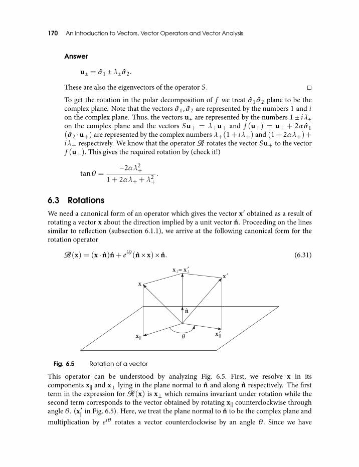
170 An Introduction to Vectors, Vector Operators and Vector Analysis
Answer
u± = σ1 ±λ±σ2.
These are also the eigenvectors of the operator S.
To get the rotation in the polar decomposition of f we treat σ1σ2 plane to be thecomplex plane. Note that the vectors σ1, σ2 are represented by the numbers 1 and ion the complex plane. Thus, the vectors u± are represented by the numbers 1 ± iλ±on the complex plane and the vectors Su+ = λ+u+ and f (u+) = u+ + 2ασ1(σ2 ·u+) are represented by the complex numbers λ+(1+ iλ+) and (1+2αλ+)+iλ+ respectively. We know that the operatorR rotates the vector Su+ to the vectorf (u+). This gives the required rotation by (check it!)
tanθ =−2αλ2
+
1+ 2αλ+ +λ2+
.
6.3 RotationsWe need a canonical form of an operator which gives the vector x′ obtained as a result ofrotating a vector x about the direction implied by a unit vector n. Proceeding on the linessimilar to reflection (subsection 6.1.1), we arrive at the following canonical form for therotation operator
R(x) = (x · n)n+ eiθ(n× x)× n. (6.31)
Fig. 6.5 Rotation of a vector
This operator can be understood by analyzing Fig. 6.5. First, we resolve x in itscomponents x‖ and x⊥ lying in the plane normal to n and along n respectively. The firstterm in the expression forR(x) is x⊥ which remains invariant under rotation while thesecond term corresponds to the vector obtained by rotating x‖ counterclockwise throughangle θ. (x′‖ in Fig. 6.5). Here, we treat the plane normal to n to be the complex plane andmultiplication by eiθ rotates a vector counterclockwise by an angle θ. Since we have

Rotations and Reflections 171
introduced a complex coefficient in the expression for the operator, the rule for theinvariance of the scalar product has to be replaced by
f ∗x · f y = x · y. (6.32)
where f ∗ is obtained from f by complex conjugation. The operator f satisfying Eq. (6.32)is called unitary.
Fig. 6.6 Infinitesimal rotation δθ of x about n
Exercise Show that the operator R(x) in Eq. (6.31) satisfies Eq. (6.32). (Hint: Useidentity II).
Thus, the rotation operator in Eq. (6.31) preserves scalar products as it should. That thedeterminant ofR(x) in Eq. (6.31) is +1 can be proved along the same lines as we did forthe reflection operator. This establishes the operator R(x) in Eq. (6.31) as the rotationoperator. However, if we wish to carry on with the operator in Eq. (6.31) to get thestructure and properties of rotation, we need a general algebraic setting incorporating themultiplication of a vector by a complex number as an integral part of it. Such an algebra isthe geometric algebra which can be used to model rotations in a general and elegantmanner [10, 7, 11]. Nevertheless we can develop the theory of rotations using only thealgebra of vectors we have learnt. We proceed to do that.
We first study infinitesimal rotations and then build up finite rotations as succession ofinfinitesimal rotations. Consider an infinitesimal rotation of a vector x about the directionimplied by a unit vector n, through an angle δθ (see Fig. 6.6). The tip of vector x then movesover an infinitesimal arc length ds of a circle of radius |x|sinφ giving ds = |x|sinφδθ(Fig. 6.6). Since the circle is a smooth curve, we can choose the arc length ds generatedby the rotation to be so small that the change dx in vector x due to rotation (see Fig. 6.7)
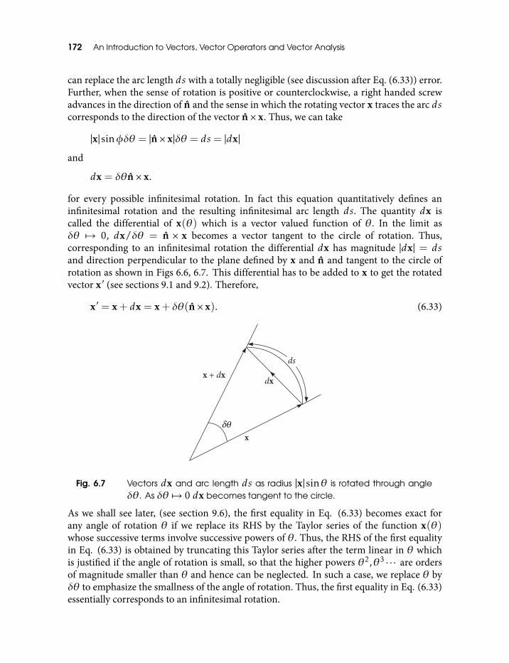
172 An Introduction to Vectors, Vector Operators and Vector Analysis
can replace the arc length ds with a totally negligible (see discussion after Eq. (6.33)) error.Further, when the sense of rotation is positive or counterclockwise, a right handed screwadvances in the direction of n and the sense in which the rotating vector x traces the arc dscorresponds to the direction of the vector n× x. Thus, we can take
|x|sinφδθ = |n× x|δθ = ds = |dx|
and
dx = δθn× x.
for every possible infinitesimal rotation. In fact this equation quantitatively defines aninfinitesimal rotation and the resulting infinitesimal arc length ds. The quantity dx iscalled the differential of x(θ) which is a vector valued function of θ. In the limit asδθ 7→ 0, dx/δθ = n × x becomes a vector tangent to the circle of rotation. Thus,corresponding to an infinitesimal rotation the differential dx has magnitude |dx| = dsand direction perpendicular to the plane defined by x and n and tangent to the circle ofrotation as shown in Figs 6.6, 6.7. This differential has to be added to x to get the rotatedvector x′ (see sections 9.1 and 9.2). Therefore,
x′ = x+ dx = x+ δθ(n× x). (6.33)
Fig. 6.7 Vectors dx and arc length ds as radius |x|sinθ is rotated through angleδθ. As δθ 7→ 0 dx becomes tangent to the circle.
As we shall see later, (see section 9.6), the first equality in Eq. (6.33) becomes exact forany angle of rotation θ if we replace its RHS by the Taylor series of the function x(θ)whose successive terms involve successive powers of θ. Thus, the RHS of the first equalityin Eq. (6.33) is obtained by truncating this Taylor series after the term linear in θ whichis justified if the angle of rotation is small, so that the higher powers θ2,θ3 · · · are ordersof magnitude smaller than θ and hence can be neglected. In such a case, we replace θ byδθ to emphasize the smallness of the angle of rotation. Thus, the first equality in Eq. (6.33)essentially corresponds to an infinitesimal rotation.
Rotations and Reflections 173
Let the vector x be rotated by an infinitesimal angle δθ1 about the direction given by aunit vector n1 to get a vector x′. Next rotate x′ through angle δθ2 about the direction givenby unit vector n2 to get the vector x′′. Using Eq. (6.33) and keeping the terms linear in δθ1and δθ2 we get (do this algebra),
x′′ = x+ δθ1(n1 × x) + δθ2(n2 × x). (6.34)
Now we reverse the order of rotations: Rotate x about n2 by δθ2 to get x′ and rotate x′
about n1 by δθ1 to get x′′. Going through the same algebra as above, keeping terms linearin δθ1 and δθ2, one can check that x′′ is again given by Eq. (6.34) which proves thatinfinitesimal rotations commute. The fact that finite rotations do not commute willbecome clear below.
Now let a vector x be rotated about a unit vector n through a finite angle θ to get avector x′. The process is depicted in Fig. 6.5. As is shown in Fig. 6.5, we resolve x into twocomponents, x‖ in the plane of rotation and x⊥ normal to this plane, i.e., in the directionof n. Rotation affects only the component x‖ while x⊥ remains invariant.
We imagine that the rotation of x‖ through θ is effected by N successive rotationsabout n, each of magnitude θ/N . We assume that N is so large (or θ/N is so small) thatEq. (6.33) applies to each of these rotations. Denote by x1,x2, . . . ,xN = x′‖ the successivelyrotated vectors. We have,
x1 =θN(n× x‖) + x‖.
x2 =θN(n× x1) + x1
=θN
n×[( θN
)n× x‖+ x‖
]+θN
n× x‖+ x‖
=
[( θN
)2n× (n× +
(2θN
)(n× + 1
]x‖).
Proceeding in this way, afterN iterations we get
x′‖ =
[(1+
(N1
)( θN
)(n×+
(N2
)( θN
)2n× (n×+ · · ·
+
(NN
)( θN
)Nn× (n× (· · ·
]x‖)
=(1 +
θN
n×)N
x‖. (6.35)
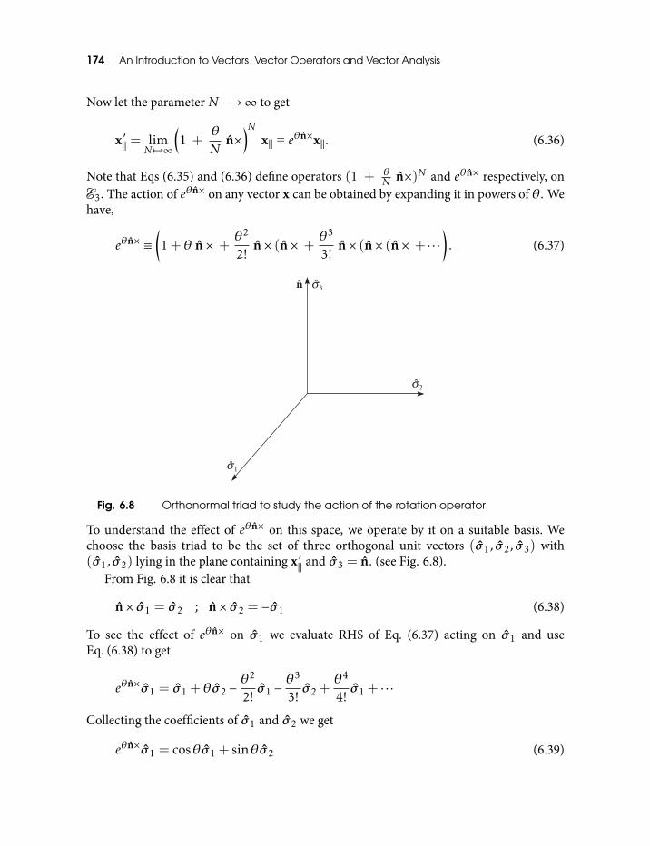
174 An Introduction to Vectors, Vector Operators and Vector Analysis
Now let the parameterN −→∞ to get
x′‖ = limN 7→∞
(1 +
θN
n×)N
x‖ ≡ eθn×x‖. (6.36)
Note that Eqs (6.35) and (6.36) define operators (1 + θN n×)N and eθn× respectively, on
E3. The action of eθn× on any vector x can be obtained by expanding it in powers of θ. Wehave,
eθn× ≡(1+θ n× +
θ2
2!n× (n× +
θ3
3!n× (n× (n× + · · ·
). (6.37)
Fig. 6.8 Orthonormal triad to study the action of the rotation operator
To understand the effect of eθn× on this space, we operate by it on a suitable basis. Wechoose the basis triad to be the set of three orthogonal unit vectors (σ1, σ2, σ3) with(σ1, σ2) lying in the plane containing x′‖ and σ3 = n. (see Fig. 6.8).
From Fig. 6.8 it is clear that
n× σ1 = σ2 ; n× σ2 = −σ1 (6.38)
To see the effect of eθn× on σ1 we evaluate RHS of Eq. (6.37) acting on σ1 and useEq. (6.38) to get
eθn×σ1 = σ1 +θσ2 −θ2
2!σ1 −
θ3
3!σ2 +
θ4
4!σ1 + · · ·
Collecting the coefficients of σ1 and σ2 we get
eθn×σ1 = cosθσ1 + sinθσ2 (6.39)
Rotations and Reflections 175
Similarly,
eθn×σ2 = −sinθσ1 + cosθσ2 (6.40)
To get the result of eθn×x‖ we resolve x‖ with respect to the basis (σ1, σ2, σ3):
x‖ = aσ1 + bσ2. (6.41)
Operating on the RHS of Eq. (6.41) by eθn× and using Eq. (6.39) and Eq. (6.40) we get
x′‖ = eθn×x‖ = (aσ1 + bσ2)cosθ+ (aσ2 − bσ1)sinθ.
By Eqs (6.38) and (6.41) this reduces to
x′‖ = eθn×x‖ = x‖ cosθ+ (n× x‖)sinθ,
or,
x′‖ = x‖+ (cosθ − 1)x‖+ sinθ(n× x‖). (6.42)
Since n is a unit vector perpendicular to x‖, we have
x‖ = −n× (n× x‖).
Substituting this in the above expression for x‖ we get
x′‖ = x‖+ (1− cosθ)n× (n× x‖) + sinθ(n× x‖).
Since x⊥ and n are parallel, we can add (n × x⊥) = 0 = n × (n × x⊥) on the RHS andx⊥(= x′⊥) on both sides of the above equation, finally giving the desired result,
x′ = x+ (1− cosθ)n× (n× x) + sinθ(n× x). (6.43)
Equation (6.43) is equivalent to the operator identity, defining the rotation operatorR
R(x) ≡ eθn×x ≡ [x+ (1− cosθ)n× (n× x) + sinθ(n× x)] . (6.44)
Exercise Show that the rotation operatorR can be equivalently expressed by
R(x) = cosθx+ (1− cosθ)(n · x)n+ sinθ(n× x). (6.45)
Hint Use identity I.
This expression for the rotation operator was used by Josiah Willard Gibbs sometime in thefirst decade of 20th century.
Exercise Show that the rotation operator as defined above is orthogonal.
176 An Introduction to Vectors, Vector Operators and Vector Analysis
Exercise Resolving x = x‖ + x⊥ with x‖ parallel and x⊥ perpendicular to n, show thatR(x) = cosθx⊥+ sinθ(n× x⊥) + x‖.
6.3.1 Matrices representing rotations
To get the matrix elements of the rotation operator on the RHS of Eqs (6.43), (6.44) wechoose an orthonormal basis (σ1, σ2, σ3) (not necessarily the same as that in Fig. 6.8)and transform each of the vectors σk,k = 1,2,3 by this operator. This will give us a newset of orthonormal vectors ek,k = 1,2,3. The matrix elements of the operator are thecoordinates of ek with respect to the basis σk. We have,
ek =3∑j=1
σ j(σ j · ek) =3∑j=1
σ jejk (6.46)
with its matrix version
[ek ]T = [σ j ]
T [ejk ] (6.47)
where [σ j ]T and [ek ]T are the row (1× 3) matrices with elements as the basis vectors σ jand ek respectively. Equation (6.46) gives, ejk = σ j · ek , or,
ejk = σ j · [σk + (1− cosθ) n× (n× σk) + sinθ n× σk ],
which reduces, via identity I to
ejk = δjk + σ j · [(n · σk)n− σk ](1− cosθ) + σ j · (n× σk)sinθ.
Let θk = n · σk denote the direction cosines of n with respect to the basis σk. We canthen write
ejk = δjk + [θjθk − δjk ](1− cosθ)− εjkmθm sinθ,
or,
ejk = δjk cosθ+θjθk(1− cosθ)− εjkmθm sinθ. (6.48)
where n =∑mθmσm and εjkm = σ j · (σk × σm) are the Levi-Civita symbols.
Thus, if n = σ3 the matrix of rotation becomescosθ −sinθ 0sinθ cosθ 0
0 0 1
. (6.49)
Note that this matrix relates the rotated vector x′ obtained by rotating the basis vectorsσ1,2 in the plane normal to n = σ3 that is, by operating the corresponding rotation
Rotations and Reflections 177
operator on x =∑k xkσk , while its transpose relates the coordinates of the same vector
with respect to σk and ek respectively.
Exercise Show that the components of x given by column vectors [x′j ] and [xj ] withrespect to the orthonormal bases ek and σk respectively are related by
[x′k ] = [ejk ]T [xj ]
where [ejk ] is the matrix defined by the rotation about n = σ3.
Solution Note that x = x′1e1 + x′2e2 + x
′3e3 = x′1R σ1 + x
′2R σ2 + x
′3R σ3. This gives,
using Eq. (6.46),
x =∑j
∑k
x′kejk
σ jor,
xj =∑k
x′kejk
or,
[x′k ] = [ejk ]T [xj ] (6.50)
where we have used [ejk ]−1 = [ejk ]
T since [ejk ] is orthogonal.
We make a few observations.It is straightforward to show (Exercise) that the rotation operatorR(n,θ) defined in
Eqs (6.43), (6.44) is an orthogonal operator, that is,
R(n,θ)x ·R(n,θ)y = x · y
for all x,y ∈ E3. This also proves that the matrix [ejk ] representingR(n,θ) is orthogonal,because we have already proved that a matrix representing an orthogonal operator isorthogonal. If we denote by S the orthogonal matrix of the rotation operator defined byEq. (6.48), then the orthogonality condition means,
ST S = I = SST or ST = S−1, (6.51)
where I is the unit matrix of size 3× 3.The determinant of the orthogonal matrix representing a rotation is +1. First, it is
straightforward to show that the determinant of the rotation operatorR(n,θ) defined inEqs (6.43), (6.44) is +1, that is,
R(n,θ)σ1 · (R(n,θ)σ2 ×R(n,θ)σ3) = 1
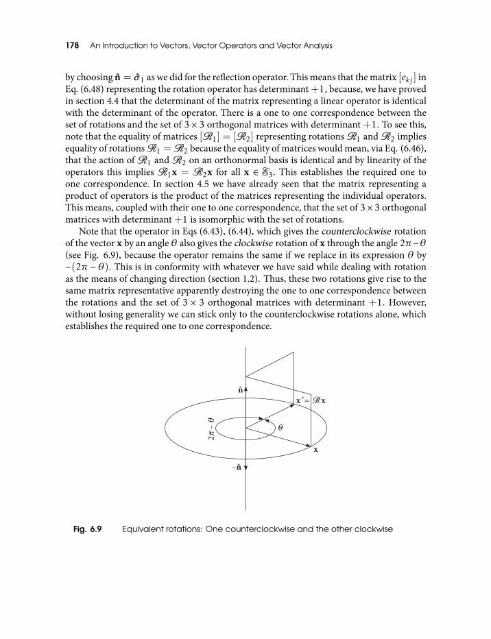
178 An Introduction to Vectors, Vector Operators and Vector Analysis
by choosing n = σ1 as we did for the reflection operator. This means that the matrix [ekj ] inEq. (6.48) representing the rotation operator has determinant +1, because, we have provedin section 4.4 that the determinant of the matrix representing a linear operator is identicalwith the determinant of the operator. There is a one to one correspondence between theset of rotations and the set of 3× 3 orthogonal matrices with determinant +1. To see this,note that the equality of matrices [R1] = [R2] representing rotationsR1 andR2 impliesequality of rotationsR1 =R2 because the equality of matrices would mean, via Eq. (6.46),that the action ofR1 andR2 on an orthonormal basis is identical and by linearity of theoperators this implies R1x = R2x for all x ∈ E3. This establishes the required one toone correspondence. In section 4.5 we have already seen that the matrix representing aproduct of operators is the product of the matrices representing the individual operators.This means, coupled with their one to one correspondence, that the set of 3×3 orthogonalmatrices with determinant +1 is isomorphic with the set of rotations.
Note that the operator in Eqs (6.43), (6.44), which gives the counterclockwise rotationof the vector x by an angle θ also gives the clockwise rotation of x through the angle 2π−θ(see Fig. 6.9), because the operator remains the same if we replace in its expression θ by−(2π − θ). This is in conformity with whatever we have said while dealing with rotationas the means of changing direction (section 1.2). Thus, these two rotations give rise to thesame matrix representative apparently destroying the one to one correspondence betweenthe rotations and the set of 3 × 3 orthogonal matrices with determinant +1. However,without losing generality we can stick only to the counterclockwise rotations alone, whichestablishes the required one to one correspondence.
Fig. 6.9 Equivalent rotations: One counterclockwise and the other clockwise
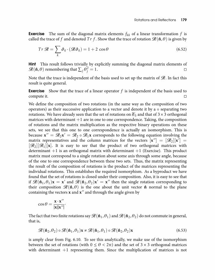
Rotations and Reflections 179
Exercise The sum of the diagonal matrix elements fkk of a linear transformation f iscalled the trace of f and denoted T r f . Show that the trace of rotationR(n,θ) is given by
T r R =∑k
σk · (R σk) = 1+ 2 cosθ (6.52)
Hint This result follows trivially by explicitly summing the diagonal matrix elements ofR(n,θ) remembering that
∑j θ
2j = 1.
Note that the trace is independent of the basis used to set up the matrix ofR . In fact thisresult is quite general.
Exercise Show that the trace of a linear operator f is independent of the basis used tocompute it.
We define the composition of two rotations (in the same way as the composition of twooperators) as their successive application to a vector and denote it by a separating tworotations. We have already seen that the set of rotations on E3 and that of 3×3 orthogonalmatrices with determinant +1 are in one to one correspondence. Taking, the compositionof rotations and the matrix multiplication as the respective binary operations on thesesets, we see that this one to one correspondence is actually an isomorphism. This isbecause x′′ = R2x′ = R2 R1x corresponds to the following equation involving thematrix representatives and the column matrices for the vectors [x′′] = [R2][x′] =[R2][R1][x]. It is easy to see that the product of two orthogonal matrices withdeterminant +1 is an orthogonal matrix with determinant +1 (Exercise). This productmatrix must correspond to a single rotation about some axis through some angle, becauseof the one to one correspondence between these two sets. Thus, the matrix representingthe result of the composition of rotations is the product of the matrices representing theindividual rotations. This establishes the required isomorphism. As a byproduct we havefound that the set of rotations is closed under their composition. Also, it is easy to see thatif R(n1,θ1)x = x′ and R(n2,θ2)x′ = x′′ then the single rotation corresponding totheir composition R(n,θ) is the one about the unit vector n normal to the planecontaining the vectors x and x′′ and through the angle given by
cosθ =x · x′′
|x||x′′ |·
The fact that two finite rotations sayR(n1,θ1) andR(n2,θ2) do not commute in general,that is,
R(n2,θ2) R(n1,θ1)x ,R(n1,θ1) R(n2,θ2)x (6.53)
is amply clear from Fig. 6.10. To see this analytically, we make use of the isomorphismbetween the set of rotations (with 0 ≤ θ < 2π) and the set of 3 × 3 orthogonal matriceswith determinant +1 representing them. Since the multiplication of matrices is not
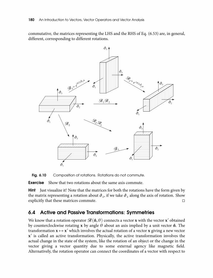
180 An Introduction to Vectors, Vector Operators and Vector Analysis
commutative, the matrices representing the LHS and the RHS of Eq. (6.53) are, in general,different, corresponding to different rotations.
Fig. 6.10 Composition of rotations. Rotations do not commute.
Exercise Show that two rotations about the same axis commute.
Hint Just visualize it! Note that the matrices for both the rotations have the form given bythe matrix representing a rotation about σ z, if we take σ z along the axis of rotation. Showexplicitly that these matrices commute.
6.4 Active and Passive Transformations: SymmetriesWe know that a rotation operatorR(n,θ) connects a vector x with the vector x′ obtainedby counterclockwise rotating x by angle θ about an axis implied by a unit vector n. Thetransformation x 7→ x′ which involves the actual rotation of a vector x giving a new vectorx′ is called an active transformation. Physically, the active transformation involves theactual change in the state of the system, like the rotation of an object or the change in thevector giving a vector quantity due to some external agency like magnetic field.Alternatively, the rotation operator can connect the coordinates of a vector with respect to
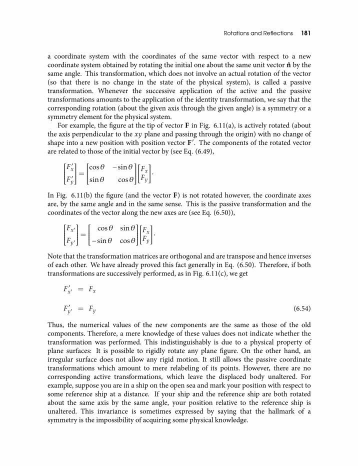
Rotations and Reflections 181
a coordinate system with the coordinates of the same vector with respect to a newcoordinate system obtained by rotating the initial one about the same unit vector n by thesame angle. This transformation, which does not involve an actual rotation of the vector(so that there is no change in the state of the physical system), is called a passivetransformation. Whenever the successive application of the active and the passivetransformations amounts to the application of the identity transformation, we say that thecorresponding rotation (about the given axis through the given angle) is a symmetry or asymmetry element for the physical system.
For example, the figure at the tip of vector F in Fig. 6.11(a), is actively rotated (aboutthe axis perpendicular to the xy plane and passing through the origin) with no change ofshape into a new position with position vector F′ . The components of the rotated vectorare related to those of the initial vector by (see Eq. (6.49),F′xF′y
= cosθ −sinθ
sinθ cosθ
[FxFy]·
In Fig. 6.11(b) the figure (and the vector F) is not rotated however, the coordinate axesare, by the same angle and in the same sense. This is the passive transformation and thecoordinates of the vector along the new axes are (see Eq. (6.50)),Fx′Fy′
= cosθ sinθ
−sinθ cosθ
[FxFy]·
Note that the transformation matrices are orthogonal and are transpose and hence inversesof each other. We have already proved this fact generally in Eq. (6.50). Therefore, if bothtransformations are successively performed, as in Fig. 6.11(c), we get
F′x′ = Fx
F′y′ = Fy (6.54)
Thus, the numerical values of the new components are the same as those of the oldcomponents. Therefore, a mere knowledge of these values does not indicate whether thetransformation was performed. This indistinguishably is due to a physical property ofplane surfaces: It is possible to rigidly rotate any plane figure. On the other hand, anirregular surface does not allow any rigid motion. It still allows the passive coordinatetransformations which amount to mere relabeling of its points. However, there are nocorresponding active transformations, which leave the displaced body unaltered. Forexample, suppose you are in a ship on the open sea and mark your position with respect tosome reference ship at a distance. If your ship and the reference ship are both rotatedabout the same axis by the same angle, your position relative to the reference ship isunaltered. This invariance is sometimes expressed by saying that the hallmark of asymmetry is the impossibility of acquiring some physical knowledge.
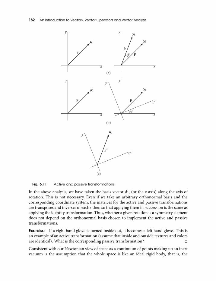
182 An Introduction to Vectors, Vector Operators and Vector Analysis
Fig. 6.11 Active and passive transformations
In the above analysis, we have taken the basis vector σ3 (or the z axis) along the axis ofrotation. This is not necessary. Even if we take an arbitrary orthonormal basis and thecorresponding coordinate system, the matrices for the active and passive transformationsare transposes and inverses of each other, so that applying them in succession is the same asapplying the identity transformation. Thus, whether a given rotation is a symmetry elementdoes not depend on the orthonormal basis chosen to implement the active and passivetransformations.
Exercise If a right hand glove is turned inside out, it becomes a left hand glove. This isan example of an active transformation (assume that inside and outside textures and colorsare identical). What is the corresponding passive transformation?
Consistent with our Newtonian view of space as a continuum of points making up an inertvacuum is the assumption that the whole space is like an ideal rigid body, that is, the
Rotations and Reflections 183
distance between every pair of points in space remains constant despite all events takingplace in it. Thus, when a single vector is rotated about any axis by any angle, the wholespace is rotated along with the vector. The subsequent passive transformation relabels allthe points in space to reproduce the initial situation. Therefore, for a single vector in space(which could be the position vector of a single particle in space), every possible rotation orreflection (which is equivalent to two rotations by Hamilton’s theorem), is a symmetrytransformation. If we consider a system of non-interacting particles we can apply thesymmetry transformations to each particle separately, independent of other particles, sothat the same conclusion applies to such a system. Thus, the system of non-interactingparticles such as an ideal gas possesses highest symmetry. In contrast, the symmetryelements of a figure like an equilateral triangle or a square, or a cube or a tetrahedron actonly on the points making up the figure and not on the rest of space. However, after thesuccession of the active and the passive transformations, the whole space, including thefigure, must reproduce the initial situation. This is possible, only when the activetransformation reproduces the initial configuration of the figure. Only a finite set ofrotations and reflections meets this requirement. Thus, the symmetry elements of a solidwhich leave its unit cell invariant, form a finite set. Thus, when a gas or a liquid condensesto make a solid, the symmetry of the system is drastically reduced. This phenomenon iscalled ‘symmetry breaking’. Generally, such a transition from liquid to solid phase, called aphase transition, occurs at a particular temperature at which the symmetry breaksspontaneously. Spontaneous symmetry breaking is responsible for the fact that thequantities like volume, magnetization, mole numbers of chemical species etc aremacroscopically observable, that is, these variables are time independent on the atomicscale of time and spatially homogeneous on the atomic scale of distance. On the otherhand, symmetries themselves are of far reaching significance as they give rise to all theconserved quantities like energy, angular momentum, linear momentum etc, which makethe understanding of the dynamics of the system possible. For example, the dynamics of aparticle driven by a central force is completely known because of the conservation ofenergy and angular momentum of such a particle. Further, Kepler’s laws of planetarymotion can be easily obtained using an additional conserved quantity, namely theRunge–Lenz vector. The underlying symmetries and symmetry breaking is crucial for theunderstanding of our physical world.
Exercise Find all the symmetry elements of a equilateral triangle and a square (seeFigs 7.1 and 7.2).
We now show that if the rotationsR1(n1,θ1) andR2(n2,θ2) are symmetry elements fora system, then so is their composition. LetR1 rotate a vector F to F′ andR2 rotate a vectorF′ to F′′. The composite rotation R12(n,θ) = R2(n2,θ2) R1(n1,θ1) must rotate Fto F′′. The matrix for the corresponding active transformation is the product [R2][R1]and that for the passive transformation is the inverse of this product. Thus, applying thecomposite active and passive transformation gives us the identity transformation. Thisproves the result.
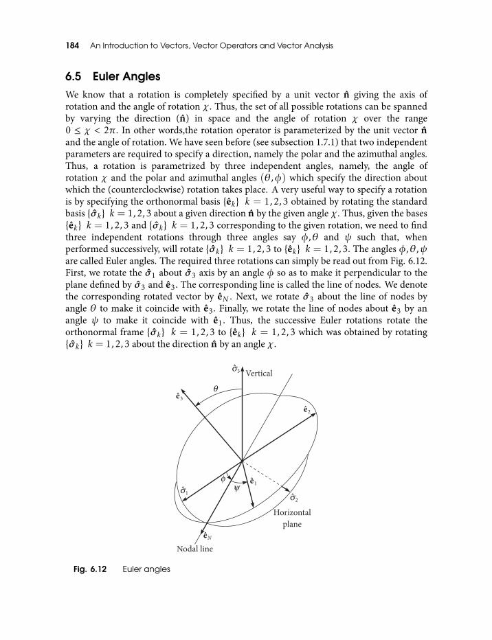
184 An Introduction to Vectors, Vector Operators and Vector Analysis
6.5 Euler AnglesWe know that a rotation is completely specified by a unit vector n giving the axis ofrotation and the angle of rotation χ. Thus, the set of all possible rotations can be spannedby varying the direction (n) in space and the angle of rotation χ over the range0 ≤ χ < 2π. In other words,the rotation operator is parameterized by the unit vector nand the angle of rotation. We have seen before (see subsection 1.7.1) that two independentparameters are required to specify a direction, namely the polar and the azimuthal angles.Thus, a rotation is parametrized by three independent angles, namely, the angle ofrotation χ and the polar and azimuthal angles (θ,φ) which specify the direction aboutwhich the (counterclockwise) rotation takes place. A very useful way to specify a rotationis by specifying the orthonormal basis ek k = 1,2,3 obtained by rotating the standardbasis σk k = 1,2,3 about a given direction n by the given angle χ. Thus, given the basesek k = 1,2,3 and σk k = 1,2,3 corresponding to the given rotation, we need to findthree independent rotations through three angles say φ,θ and ψ such that, whenperformed successively, will rotate σk k = 1,2,3 to ek k = 1,2,3. The angles φ,θ,ψare called Euler angles. The required three rotations can simply be read out from Fig. 6.12.First, we rotate the σ1 about σ3 axis by an angle φ so as to make it perpendicular to theplane defined by σ3 and e3. The corresponding line is called the line of nodes. We denotethe corresponding rotated vector by eN . Next, we rotate σ3 about the line of nodes byangle θ to make it coincide with e3. Finally, we rotate the line of nodes about e3 by anangle ψ to make it coincide with e1. Thus, the successive Euler rotations rotate theorthonormal frame σk k = 1,2,3 to ek k = 1,2,3 which was obtained by rotatingσk k = 1,2,3 about the direction n by an angle χ.
Fig. 6.12 Euler angles
Rotations and Reflections 185
Thus, to every triple of Euler anglesφ,θ,ψ the above construction associates a rotationof 3-D space taking frame σk k = 1,2,3 into the frame ek k = 1,2,3. The ranges ofthe Euler angles are
0 < φ < 2π, 0 < ψ < 2π, 0 < θ < π.
Thus, by continuously varying the Euler angles, we can generate all possible rotations.Thus, the set of all possible rotations about a point is parameterized by three Euler anglesvarying in their specified ranges.
The net rotation is given by the composition of Euler rotations in the order stated above.We have,
R(n,χ) = eψe3×eθeN×eφσ3× (6.55)
Exercise Show that the line of nodes has the direction
eN = eθeN×σ1 =σ3 × e3
|σ3 × e3|.
Let us now set up the matrix representingR(n,χ) in terms of its Euler angles. To do this,we have to expand the vectors ek k = 1,2,3 in terms of the basis σk k = 1,2,3. To gete3 we have to first evaluate eφσ3×σ1 and then evaluate eφn×σ3 where n = eφσ3×σ1 usingEq. (6.43) or Eq. (6.45). Carrying out this calculation we get,
e3 = sinθ sinφσ1 − sinθ cosφσ2 + cosθσ3.
Evaluating e1 and e2 in the same way, we get, for the matrix representingR(n,χ) in termsof its Euler angles,
cosψ cosφ− sinψ sinφcosθ −sinψ cosφ− cosψ sinφcosθ sinθ sinφcosψ sinφ+ sinψ cosφcosθ −sinψ sinφ+ cosψ cosφcosθ −sinθ cosφ
sinθ sinψ sinθ cosψ cosθ
·If we multiply the row vector [σ1σ2σ3] on the right by this matrix, then we get the rowvector [e1e2e3]. The Euler rotations corresponding to arbitrary rotation, defined above,are marred by the fact that their axes of rotation are not fixed directions in space. We candefine Euler rotations using a construction by which every rotationR(n,χ) is reduced toa composition of rotations about fixed axes of a standard basis. In this construction, anarbitrary rotation is decomposed into Euler rotations as
R =R(n,χ) = eφσ3×eθσ1×eψσ3× =RφRθRψsay (6.56)
Thus, the first rotation is about σ3 by an angleψ the second rotation is about σ1 by an angleθ and the third one is about σ3 by an angle φ. Note that ek =R σk =RφRθRψσk sothat it is quite easy to calculate the matrix elements of a rotation in terms of Euler angles.
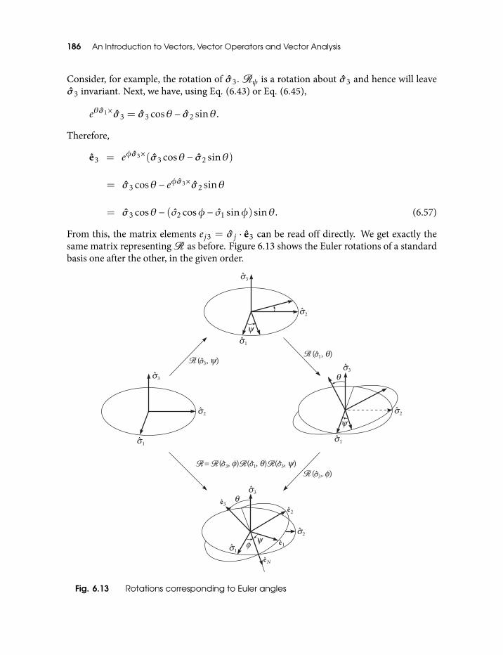
186 An Introduction to Vectors, Vector Operators and Vector Analysis
Consider, for example, the rotation of σ3.Rψ is a rotation about σ3 and hence will leaveσ3 invariant. Next, we have, using Eq. (6.43) or Eq. (6.45),
eθσ1×σ3 = σ3 cosθ − σ2 sinθ.
Therefore,
e3 = eφσ3×(σ3 cosθ − σ2 sinθ)
= σ3 cosθ − eφσ3×σ2 sinθ
= σ3 cosθ − (σ2 cosφ− σ1 sinφ)sinθ. (6.57)
From this, the matrix elements ej3 = σ j · e3 can be read off directly. We get exactly thesame matrix representingR as before. Figure 6.13 shows the Euler rotations of a standardbasis one after the other, in the given order.
Fig. 6.13 Rotations corresponding to Euler angles
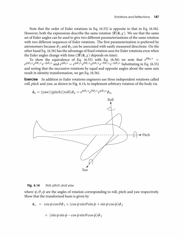
Rotations and Reflections 187
Note that the order of Euler rotations in Eq. (6.55) is opposite to that in Eq. (6.56).However, both the expressions describe the same rotationR(n,χ). We see that the sameset of Euler angles can be used to give two different parameterizations of the same rotationwith two different sequences of Euler rotations. The first parameterization is preferred byastronomers because σ3 and e3 can be associated with easily measured directions. On theother hand Eq. (6.56) has the advantage of fixed rotation axes for Euler rotations even whenthe Euler angles change with time (R(n,χ) depends on time).
To show the equivalence of Eq. (6.55) with Eq. (6.56) we note that eθeN× =eφσ3×eθσ1×e−φσ3× and eψe3× = eφσ3×eθσ1×eψσ3×e−θσ1×e−φσ3× Substituting in Eq. (6.55)and noting that the successive rotations by equal and opposite angles about the same axisresult in identity transformation, we get Eq. (6.56).
Exercise In addition to Euler rotations engineers use three independent rotations calledroll, pitch and yaw, as shown in Fig. 6.14, to implement arbitrary rotation of the body via
ek = (yaw)(pitch)(roll)σk = eφσ1×eθσ2×eψσ3×σk ,
Fig. 6.14 Roll, pitch and yaw
where ψ,θ,φ are the angles of rotation corresponding to roll, pitch and yaw respectively.Show that the transformed basis is given by
e1 = cosψ cosθσ1 + (cosψ sinθ sinφ+ sinψ cosφ)σ2
+ (sinψ sinφ− cosψ sinθ cosφ)σ3
188 An Introduction to Vectors, Vector Operators and Vector Analysis
e2 = −sinψ cosθσ1 + (cosψ cosφ− sinψ sinθ sinφ)σ2
+ (cosψ sinφ+ sinψ sinθ cosφ)σ3
e3 = sinθσ1 − cosθ sinφσ2 + cosθ cosφσ3 (6.58)
Write down the matrix for the corresponding rotation.
6.6 Euler’s TheoremIn section 6.3, we analyzed a rotation about a given axis and found the orthogonal matrixof the corresponding rotation operator with respect to an arbitrary orthonormal basis. Wenow do the reverse: Given a 3 × 3 orthogonal real matrix [R ] with determinant +1, weshow that the transformation [x] 7→ [R ][x] ; x ∈ E3 can be realized by first choosinga fixed direction in space through the origin and then rotating x through a suitable angleabout this direction as the axis. This is known as Euler’s theorem. Henceforth in this section,we will use the same symbol for the rotation operator and the matrix representing it andalso for the vectors and the corresponding 3×1 column vectors, because in this section, wewill be exclusively dealing with matrices.
Let λi and vi , (i = 1,2,3) denote the eigenvalues and eigenvectors ofR which maybe complex, althoughR is real. These satisfy the equations
Rvi = λivi (i = 1,2,3). (6.59)
Since R is an orthogonal matrix, we have (see section 6.1) ‖Rvi‖ = ‖vi‖ where for anyvector v, ‖v‖ denotes the Euclidean length (|vx|2 + |vy |2 + |vz|2)1/2. Therefore, byEq. (6.59),
|λi |= 1 (i = 1,2,3). (6.60)
The λis are the roots of the real cubic equation
det(λI −R) = 0. (6.61)
The product of the roots is
λ1λ2λ3 = det R = 1. (6.62)
At least one of the roots is real. To see this note that for large enough |λ|, the cubic termdominates, so that the sign of the cubic polynomial in Eq. (6.61) is the same as that of λ.This means that the graph of the cubic polynomial (which is a continuous function) hasto cut the λ axis at least once. If the other two eigenvalues (say λ2,λ3) are complex, thenλ3 = λ∗2 (superfix ∗ denotes complex conjugation) and by Eq. (6.60) λ2λ3 = 1, hence by
Rotations and Reflections 189
Eq. (6.62) λ1 = 1. If all the three roots are real, they can be (1,1,1) or (1,−1,−1). In anycase there is always one root, say λ1, equal to +1, hence
Rv1 = v1 (6.63)
which shows that the straight line through the origin in the direction of v1, is invariantunder the transformation x 7→Rx. Obviously, this is the axis of rotation.
Let λ1 = 1, λ2 = eiθ, λ3 = e−iθ and let v1,v2,v3 form an orthonormal set. Theeigenvectors of a orthogonal matrix can always be orthonormalized. Call
u1 = v1
u2 =1√
2(v2 + v3)
u3 =i√
2(v2 − v3). (6.64)
uis form a orthonormal set (check it!) and can be taken to be real, because v2 and v3can be taken to be complex conjugates.2 From Eq. (6.64) and the values of λi i = 1,2,3we get,
Ru1 = u1
Ru2 = cosθu2 + sinθu3
Ru3 = −sinθu2 + cosθu3. (6.65)
We see that the transformationR is a rotation in the plane perpendicular to u1.When the matrix R is given, the corresponding angle and axis of rotation can be
obtained as follows. Since the sum of the eigenvalues of a matrix equals its trace, the angleθ is given by
1+ eiθ + e−iθ =R11 +R22 +R33,
or,
cosθ =12(R11 +R22 +R33 − 1) .
Let the axis of rotation be in the direction of the eigenvector v, that corresponds to theeigenvalue λ= 1, so thatRv = v. SinceR is orthogonal,RTR = I , hence v =RT v.
2Just take the complex conjugate ofRv2 = λ2v2 and compare withRv3 = λ3v3 noting that λ3 = λ∗2.
190 An Introduction to Vectors, Vector Operators and Vector Analysis
Therefore, (R −RT )v = 0 which is a homogeneous system of simultaneous linearequations in the components v1,v2,v3 of v. Thus, the components of v are in the ratio
v1 : v2 : v3 = (R23 −R32) : (R31 −R13) : (R12 −R21) . (6.66)
Exercise Establish Eq. (6.66).
In many cases the matrix of the rotation operator with respect to some basis is what isknown, so we have to carry out the procedure in this section in order to get the specificrotation represented by the matrix. Such a specification is required in order to get thekinematical and dynamical description of a rotating physical system.
7
Transformation Groups
7.1 Definition and ExamplesA state of a physical system at a time t is given by specifying the values of different vector(and scalar) physical quantities pertaining to the system at that time. The values of thevector physical quantities form a part of E3. Thus, the action of an operator ortransformation on E3 will, in general, change the state of the system. Thus, all possiblechanges in the state correspond to a collection of transformations on E3. Such a set oftransformations may form an extremely important algebraic structure called a group. Theevolution of a system in time, due to its interaction with other systems, is controlled by itsLagrangian (or Hamiltonian). The symmetry element of the system, which leaves itsLagrangian (or Hamiltonian) invariant, gives rise to a conservation law, that is, it gives riseto an expression involving the position and momentum vectors of the system, whose valueremains the same at all times, throughout the motion of the system. This result is calledNoether’s theorem. The set of all such symmetry elements form a group. This fact turnsout to be of great advantage in the theoretical development of mechanics, quantummechanics and of physics in general. In fact whole of mechanics can be developed fromthe group theoretical point of view, as in the book by N. Mukunda and E. C. G. Sudarshan[22]. Here our intention is to give elementary group theory with an emphasis on therotation group and the group of isometries over E3 (also called Euclidean group) with aview to understand rigid body motion, which is a combination of the rotational andtranslational motion.
A group G is any set of elements a,b,c, . . . ,x,y,z, . . ., finite or infinite, together withthe law of composition, denoted , such that
(i) (Closure) If a and b are any two elements of G, then a b is an element of G.(ii) (Associative law) If a,b,c ∈ G then
(a b) c = a (b c) (7.1)
192 An Introduction to Vectors, Vector Operators and Vector Analysis
(iii) If a,b ∈ G then there exist unique elements x,y ∈ G such that
a x = b and y a = b (7.2)
If the elements are numbers, vectors, matrices etc, the composition abmay either bethe sum or the product of a and b. In the case of mappings, transformations, rotations,permutations. etc, the law is understood to be the usual law of composition; if a,b aretransformations, then a b is the transformation which results from performing bfirst, then a.
Exercise Show that the set of all rotations in a plane Rφ : 0 ≤ φ < 2π forms agroup.
Hint All the rotations are about the same axis, perpendicular to the plane, so thatRφ1
Rφ2=Rφ1+φ2
.
Exercise Prove the following laws which are the consequences of axioms (i), (ii),(iii) above.
(iv) (Law of cancellation) If a,b,c ∈ G then
a b = a c implies b = c
b a = c a implies b = c (7.3)
Hint Use axiom (iii) and the fact that the elements x and y defined in (iii) are unique.(v) (Identity) There is a unique element e ∈ G such that
a e = a= e a
for all a ∈ G.
Hint Use (iii) with b replaced by a to get
a e = a e′ a = a.
To show that e = e′ put a= e and use the law of cancellation.(vi) (Inverse) For every a ∈ G, there exists a unique a−1 ∈ G such that
a−1 a= e = a a−1.
(vii) (Extended associative law)
(a (b (c (· · · ))) · · · ) h= a b c · · · h
so that unnecessary parentheses can be omitted.(viii) (Extended inverse) (a b c · · · x y)−1 = y−1 x−1 · · · b−1 a−1.
Transformation Groups 193
Note that the law of composition need not be commutative, that is, in general, ab , ba.a,b ∈ G are said to commute if a b = b a. If all pairs of elements of G commute, then Gis said to be commutative or Abelian.
Let a ∈ G andm ≥ 0 be an integer. Then, am is defined as follows.
a0 = e, a1 = a, a2 = a a, a3 = a2 a, . . . , am = am−1 a; a−m = (a−1)m
If all the elements an (n = 0,±1,±2, · · · ) are distinct, then the element a is said to be ofinfinite order, otherwise, there is a smallest positive integer l, called the order of a, suchthat al = e. Then, am = e provided l is a divisor of m and every power of a equals oneof the elements e,a,a2, . . . ,al−1. The group comprising e,a,a2, . . . ,al−1 is called the cyclicgroup of l elements.
If a subset G′ ⊆ G of a group G is a group with the same law of composition as G, it iscalled a subgroup of G. For example, the rotations about a fixed axis form a subgroup ofthe group of rotations on E3. The distinct powers of an element a form a subgroup called asubgroup generated by the element a. This could be the cyclic subgroup of finite or infiniteorder. The order of a group is the number of elements in it which can be finite or infinite.If G′ is a subgroup of G we write G′ < G. In any case, G < G and e < G. If G′ , G, G′ is aproper subgroup, If G′ = e, G′ is a trivial subgroup.
Examples
(i) The vector space E3 is an additive Abelian group containing infinite elements. This isobvious from the properties of vector addition listed in section 1.4.
(ii) Let G denote the following set of 2× 2 real matrices,
e =
(1 00 1
)a=
(0 −11 0
)b =
(−1 00 −1
)c =
(0 1−1 0
)·
It is straightforward to check that this set forms a group under matrix multiplication.For example, a c = e and a−1 = c.
(iii) Let C4 denote the group of the rotational symmetries of a square, under thecomposition of rotations, namely,
e = identity (rotation through 0)a= counterclockwise rotation through π/2b = counterclockwise rotation through πa= counterclockwise rotation through 3π/2 (clockwise rotation through π/2)
Exercise Show that the groups in examples (ii) and (iii) are simply two differentrealizations of ‘cyclic group of four elements’.
(iv) The sets Z2 of integers modulo 2 and ((1,−1), ·) are groups under the respectivebinary operations and are isomorphic. We name them Z2 and C2 respectively. Bothare cyclic groups of two elements e,a with a2 = e. The three element group C3 is
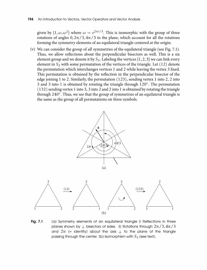
194 An Introduction to Vectors, Vector Operators and Vector Analysis
given by 1,ω,ω2 where ω = e2πi/3. This is isomorphic with the group of threerotations of angles 0,2π/3,4π/3 in the plane, which account for all the rotationsforming the symmetry elements of an equilateral triangle centered at the origin.
(v) We can consider the group of all symmetries of the equilateral triangle (see Fig. 7.1).Thus, we allow reflections about the perpendicular bisectors as well. This is a sixelement group and we denote it by S3. Labeling the vertices 1,2,3we can link everyelement in S3 with some permutation of the vertices of the triangle. Let (12) denotethe permutation which interchanges vertices 1 and 2 while leaving the vertex 3 fixed.This permutation is obtained by the reflection in the perpendicular bisector of theedge joining 1 to 2. Similarly, the permutation (123), sending vertex 1 into 2, 2 into3 and 3 into 1 is obtained by rotating the triangle through 120. The permutation(132) sending vertex 1 into 3, 3 into 2 and 2 into 1 is obtained by rotating the trianglethrough 240. Thus, we see that the group of symmetries of an equilateral triangle isthe same as the group of all permutations on three symbols.
Fig. 7.1 (a) Symmetry elements of an equilateral triangle i) Reflections in threeplanes shown by ⊥ bisectors of sides. ii) Rotations through 2π/3,4π/3and 2π (= identity) about the axis ⊥ to the plane of the trianglepassing through the center. (b) Isomorphism with S3 (see text).
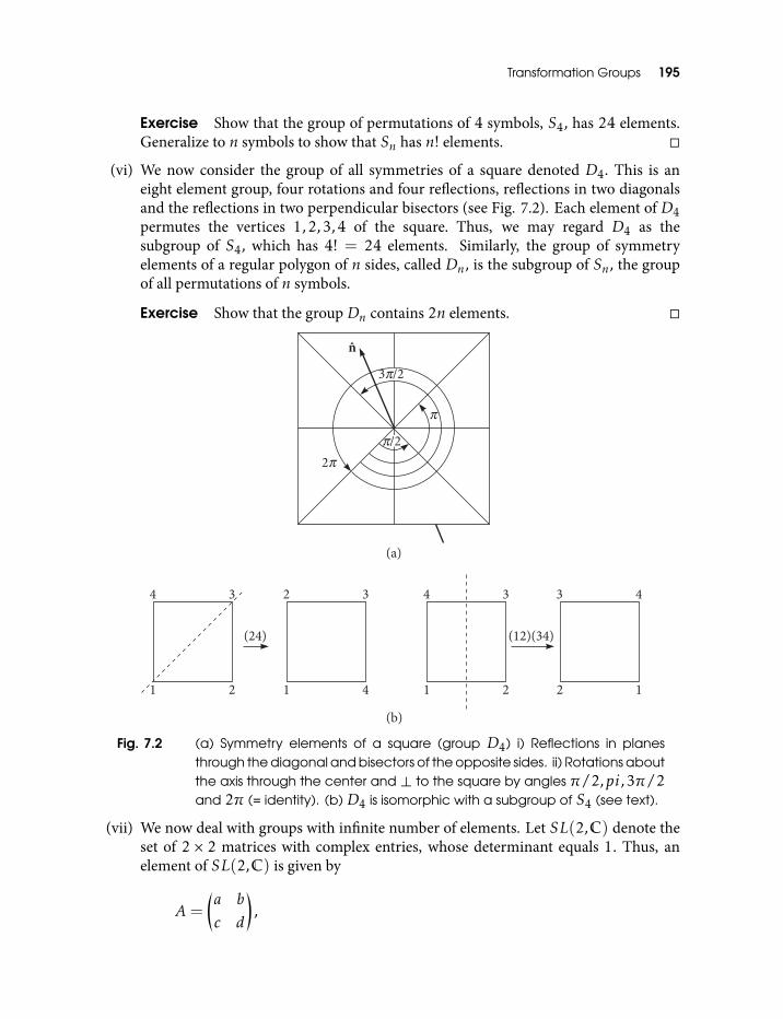
Transformation Groups 195
Exercise Show that the group of permutations of 4 symbols, S4, has 24 elements.Generalize to n symbols to show that Sn has n! elements.
(vi) We now consider the group of all symmetries of a square denoted D4. This is aneight element group, four rotations and four reflections, reflections in two diagonalsand the reflections in two perpendicular bisectors (see Fig. 7.2). Each element of D4permutes the vertices 1,2,3,4 of the square. Thus, we may regard D4 as thesubgroup of S4, which has 4! = 24 elements. Similarly, the group of symmetryelements of a regular polygon of n sides, called Dn, is the subgroup of Sn, the groupof all permutations of n symbols.
Exercise Show that the group Dn contains 2n elements.
Fig. 7.2 (a) Symmetry elements of a square (group D4) i) Reflections in planesthrough the diagonal and bisectors of the opposite sides. ii) Rotations aboutthe axis through the center and ⊥ to the square by angles π/2,pi,3π/2and 2π (= identity). (b) D4 is isomorphic with a subgroup of S4 (see text).
(vii) We now deal with groups with infinite number of elements. Let SL(2,C) denote theset of 2 × 2 matrices with complex entries, whose determinant equals 1. Thus, anelement of SL(2,C) is given by
A=
(a b
c d
),
196 An Introduction to Vectors, Vector Operators and Vector Analysis
where a,b,c,d are complex numbers satisfying
ad − bc = 1.
Exercise Show that SL(2,C) forms a non-commutative group under matrixmultiplication.
Hint Since the determinant of the product of matrices is the product of theirdeterminants, SL(2,C) is closed under matrix multiplication. Further, matrixproduct is associative. Since det A= 1, A is invertible, and det A−1 = 1/det A= 1,implying A−1 exists and is in SL(2,C). The identity is given by
e =
(1 00 1
)·
(viii) SU (n) denotes the set of all n×n unitary matrices with determinant 1 and is a groupunder matrix multiplication. SU (n) is closed under matrix multiplication becausegiven two unitary matricesU1,U2 we see that their product is also unitary,
(U1U2)† = U†2U
†1 = U−1
2 U−11 = (U1U2)
−1 (7.4)
and the determinant of the product of matrices is the product of their determinants.Further, matrix product is associative. Unit n× n matrix, which is the multiplicativeidentity, is unitary.
For example, the group SU (2) consists of all 2× 2 matrices of the form(a b
−b∗ a∗
), where |a|2 + |b|2 = 1.
The superscript ∗ corresponds to complex conjugation.Given a group G, a group G′ homomorphic to G is called a representation of G. If
a representation is isomorphic to G, it is called a faithful representation.Representation of groups by multiplicative (or additive) groups of matrices is veryuseful, especially when the representation is faithful, or even otherwise, becausemany properties of the original group can be obtained by studying thecorresponding group of matrices which is, generally, much easier to do.
Exercise Show that the set of all orthogonal matrices with determinant +1 formsa group.
7.2 The Rotation Group O +(3)
We have already seen that the composition of two counterclockwise rotations is acounterclockwise rotation. Thus, the set of all rotations on E3 is closed under the
Transformation Groups 197
composition of rotations. The composition of rotations is associative because by itsdefinition, both the compositions (R1 R2) R3 and R1 (R2 R3) can beimplemented in only one way, namely, by applying the individual rotations in the orderR3,R2,R1 in succession. The rotation with zero angle of rotation is the identityrotation, which does not rotate anything at all, so that its composition with any otherrotation gives back the same rotation. The inverse of a rotationR(n,θ) isR(n,2π −θ).Thus, the set of all possible rotations on E3 is a group under the composition of rotations,called O +(3). All the rotations in O +(3) together leave one point in space invariant, apoint which is common to all the axes of rotation, taken to be the origin. Physically, abody which is only rotating has to leave at least one point in it undisplaced or stationarybecause the displacement of all points in the body corresponds to the translation of thewhole body. Note that this group is not only infinite but is uncountable. In fact, it isparameterized by three Euler angles and can be scanned by continuously varying theseparameters covering their ranges. These continuous parameters scanning the group forma region in R3 and the continuous variations in these parameters correspond to differentpossible paths in this region. In particular, starting from any rotation, its three Eulerangles can be continuously reduced to zero to reach the identity. Thus, every rotationoperator is continuously connected to the identity element e0n× = I corresponding tozero rotation. Because of this property, the group of rotations, O +(3), is called acontinuous group.
We have seen that, having chosen an orthonormal basis σk k = 1,2,3 in E3, a matrixrepresenting every rotationR(n,θ) is given by
ejk = σ j ·R σk ,
where ejk is the jkth element of the matrix. By subsection 6.3.1 we know that every suchmatrix is a 3×3 orthogonal matrix with determinant +1 and that the sets of rotations andtheir matrix representatives are isomorphic. The last exercise tells us that the set of allorthogonal matrices with determinant +1 is a group under matrix multiplication whichwe call SO(3). All this just means that the group of 3 × 3 matrices with determinant +1,SO(3), is a faithful matrix representation of the rotation group O +(3). Thus, these twogroups have the same structure and properties and it is enough to study SO(3) tounderstand rotations in E3. In fact each 3 × 3 real matrix A defines a linear mapf : x 7→ Ax on E3, so that, by the isomorphism between SO(3) and O +(3), the groupformed by the maps x 7→ Ax with A ∈ SO(3) is just O +(3). Since O +(3) is a threeparameter continuous group, so must be the isomorphic group SO(3).
Exercise Show that SO(3) is a three parameter group.
Solution The conditions of orthogonality on a 3× 3 matrix A= [akj ] are, by Eq. (6.7),
3∑k=1
a2kj = 1 (j = 1,2,3)
198 An Introduction to Vectors, Vector Operators and Vector Analysis
3∑k=1
akiakj = 0 (i, j) = (1,2), (1,3), (2,3) (7.5)
amounting to 6 constraints to be satisfied by 9 elements of the 3 × 3 matrix. This leavesonly 3 independent parameters out of 9 elements of A. Actually we have not counted theconstraint det A= 1. However, it turns out that this constraint does not reduce the numberof independent parameters, but eliminates all the matrices with determinant −1 from theparent set of orthogonal matrices with determinant ±1.
The set of all orthogonal transformations on E3 forms a group. We know that the setof orthogonal transformations is partitioned into two classes, characterized bytransformations with determinant ±1 corresponding to rotations and reflectionsrespectively. The composition of two rotations is a rotation while the composition of tworeflections is a rotation by Hamilton’s theorem (subsection 6.1.2). Thus, the compositionof two orthogonal transformations is an orthogonal transformation. The composition ofrotations is associative and by the same argument the composition of reflections is alsoassociative. Thus, the composition of orthogonal transformations is associative. Theinverse of an orthogonal transformation is uniquely given by its adjoint. Finally,the identity transformation is orthogonal. This makes the set of all orthogonaltransformations on E3 a group under the composition of transformations and we call itO (3). Obviously, O +(3) is a subgroup of O (3), however, the class of reflections is not,because it is not closed under the composition of reflections.
Exercise Show that the product of two orthogonal transformations (matrices) is anorthogonal transformation (matrix).
Hint Proceed as in Eq. (7.4) for unitary matrices.
In section 4.5 we proved that the matrix representing the product of two transformationsis the product of the matrices representing the factors, (in the same order). In section 6.1we showed that the matrix representing an orthogonal operator is orthogonal. By theabove exercise, the product of two orthogonal matrices is orthogonal. If two orthogonalmatrices are equal, then the corresponding orthogonal operators are equal, just as in thecase of rotations. The set of all 3 × 3 orthogonal matrices forms a group under matrixmultiplication (Exercise) also called O (3). All this just means that the group oforthogonal 3 × 3 matrices is a faithful representation of the group of orthogonaltransformations on E3. It is then enough to analyze the group of matrices O (3), in orderto get the structure and properties of the group of orthogonal transformations on E3. Infact the group of orthogonal transformations is identical to the group of linear mapsx 7→ Ax on E3 where A is a 3 × 3 orthogonal matrix. O (3) is also a continuous groupdriven by three independent parameters as we saw for its subgroup SO(3).
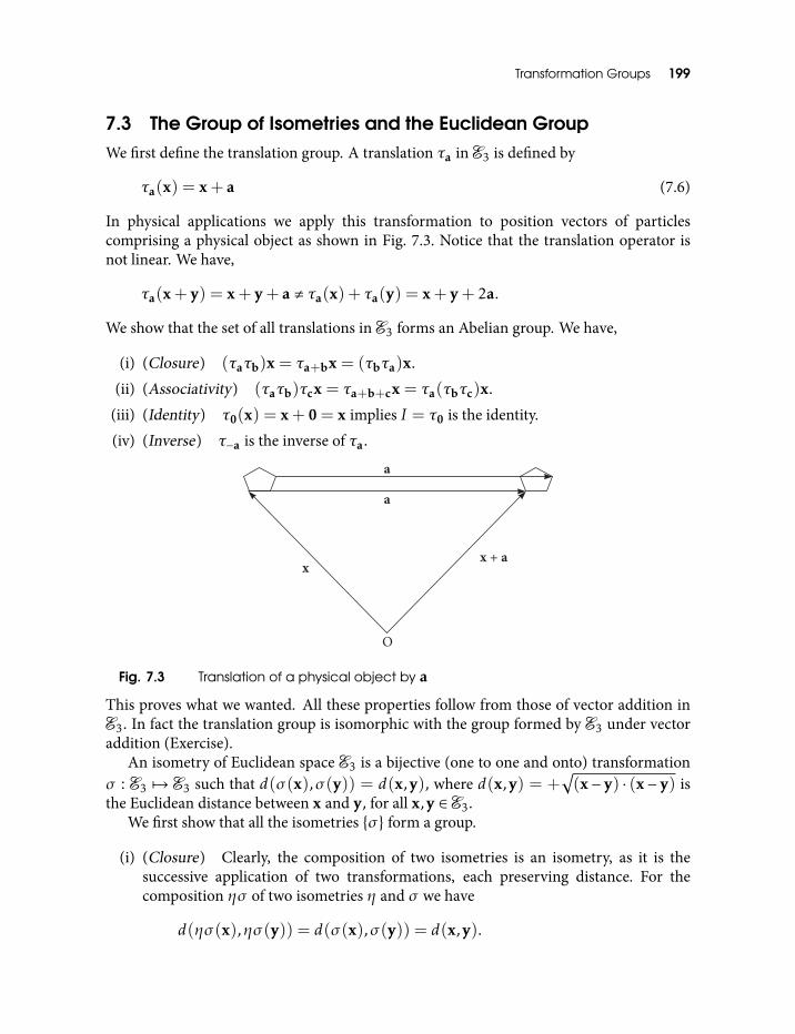
Transformation Groups 199
7.3 The Group of Isometries and the Euclidean GroupWe first define the translation group. A translation τa in E3 is defined by
τa(x) = x+ a (7.6)
In physical applications we apply this transformation to position vectors of particlescomprising a physical object as shown in Fig. 7.3. Notice that the translation operator isnot linear. We have,
τa(x+ y) = x+ y+ a , τa(x) + τa(y) = x+ y+ 2a.
We show that the set of all translations in E3 forms an Abelian group. We have,
(i) (Closure) (τaτb)x = τa+bx = (τbτa)x.
(ii) (Associativity) (τaτb)τcx = τa+b+cx = τa(τbτc)x.
(iii) (Identity) τ0(x) = x+ 0 = x implies I = τ0 is the identity.
(iv) (Inverse) τ−a is the inverse of τa.
Fig. 7.3 Translation of a physical object by a
This proves what we wanted. All these properties follow from those of vector addition inE3. In fact the translation group is isomorphic with the group formed by E3 under vectoraddition (Exercise).
An isometry of Euclidean space E3 is a bijective (one to one and onto) transformationσ : E3 7→ E3 such that d(σ (x),σ (y)) = d(x,y), where d(x,y) = +
√(x− y) · (x− y) is
the Euclidean distance between x and y, for all x,y ∈ E3.We first show that all the isometries σ form a group.
(i) (Closure) Clearly, the composition of two isometries is an isometry, as it is thesuccessive application of two transformations, each preserving distance. For thecomposition ησ of two isometries η and σ we have
d(ησ (x),ησ (y)) = d(σ (x),σ (y)) = d(x,y).
200 An Introduction to Vectors, Vector Operators and Vector Analysis
(ii) (Associativity) Let σ1,σ2,σ3 be isometries. Then, both (σ1σ2)σ3 and σ1(σ2σ3)have to be obtained by successively applying σ3,σ2,σ1 (in that order), makingthem equal.
(iii) (Identity) The identity transformation I(x) = x is an isometry.
(iv) (Inverse) By the bijection property, every isometry σ has an inverse, σ−1 and sinceσ is an isometry
d(σ−1(x),σ−1(y)) = d(σσ−1(x),σσ−1(y)) = d(x,y)
so that σ−1 is an isometry.Items (i)–(iv) above show that the set of all isometries in E3 form a group.We now obtain some of the basic properties of an isometry.Consider an orthonormal basis e1, e2, e3 and an isometry σ which leaves the vectors
0, e1, e2, e3 invariant. Then, we want to show that σ is the identity. Let x,x′ ∈ E3 andσ (x) = x′ . Since σ (0) = 0 we have d(x,0) = d(σ (x), σ (0)) = d(x′, 0). This gives,
x2 = (x′)2. (7.7)
Similarly, invariance of e1, e2, e3 under σ gives, for example,
(x− e1) · (x− e1) = (x′ − e1) · (x′ − e1)
or,
x2 − 2x · e1 + 1 = (x′)2 − 2x′ · e1 + 1 (7.8)
From Eqs (7.7) and (7.8) we get,
x = x′
or, σ (x) = x for all x ∈ E3, giving σ = I . Note that this conclusion is trivial for a linearoperator as it follows directly from linearity. However, isometry is not linear in general.
Let σ be an isometry which leaves 0 invariant, that is, σ leaves one point in E3 fixed.Then we know that σ is an orthogonal transformation. In fact from Eq. (7.7) we know thatσ (0) = 0 implies σ (x) ·σ (x) = x · x, or, σ preserves the length of vectors in E3. Hence, σis an orthogonal transformation.
Let σ be an isometry with σ (0) = a. Then
σ (x) = Ax+ a x ∈ E3 (7.9)
where A is an orthogonal transformation. To see this, define a translation τa(x) = x + a.This is an isometry with inverse τ−a(x) = x − a. Thus, τ−aσ (0) = 0 so that τ−aσ is anisometry fixing 0. Therefore, τ−aσ must be an orthogonal transformation which we denoteby A. We can then write
σ (x) = τaτ−aσ (x) = τaA(x) = A(x) + a (7.10)
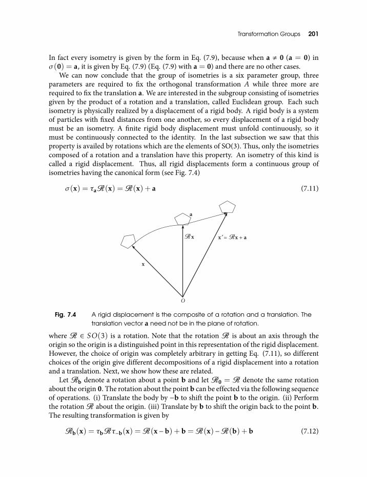
Transformation Groups 201
In fact every isometry is given by the form in Eq. (7.9), because when a , 0 (a = 0) inσ (0) = a, it is given by Eq. (7.9) (Eq. (7.9) with a = 0) and there are no other cases.
We can now conclude that the group of isometries is a six parameter group, threeparameters are required to fix the orthogonal transformation A while three more arerequired to fix the translation a. We are interested in the subgroup consisting of isometriesgiven by the product of a rotation and a translation, called Euclidean group. Each suchisometry is physically realized by a displacement of a rigid body. A rigid body is a systemof particles with fixed distances from one another, so every displacement of a rigid bodymust be an isometry. A finite rigid body displacement must unfold continuously, so itmust be continuously connected to the identity. In the last subsection we saw that thisproperty is availed by rotations which are the elements of SO(3). Thus, only the isometriescomposed of a rotation and a translation have this property. An isometry of this kind iscalled a rigid displacement. Thus, all rigid displacements form a continuous group ofisometries having the canonical form (see Fig. 7.4)
σ (x) = τaR(x) =R(x) + a (7.11)
Fig. 7.4 A rigid displacement is the composite of a rotation and a translation. Thetranslation vector a need not be in the plane of rotation.
where R ∈ SO(3) is a rotation. Note that the rotation R is about an axis through theorigin so the origin is a distinguished point in this representation of the rigid displacement.However, the choice of origin was completely arbitrary in getting Eq. (7.11), so differentchoices of the origin give different decompositions of a rigid displacement into a rotationand a translation. Next, we show how these are related.
LetRb denote a rotation about a point b and letR0 = R denote the same rotationabout the origin 0. The rotation about the point b can be effected via the following sequenceof operations. (i) Translate the body by −b to shift the point b to the origin. (ii) Performthe rotationR about the origin. (iii) Translate by b to shift the origin back to the point b.The resulting transformation is given by
Rb(x) = τbRτ−b(x) =R(x−b) +b =R(x)−R(b) +b (7.12)
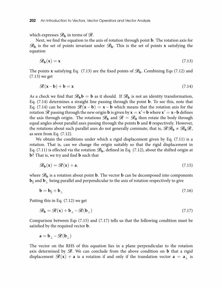
202 An Introduction to Vectors, Vector Operators and Vector Analysis
which expressesRb in terms ofR .Next, we find the equation to the axis of rotation through point b. The rotation axis for
Rb is the set of points invariant under Rb. This is the set of points x satisfying theequation
Rb(x) = x (7.13)
The points x satisfying Eq. (7.13) are the fixed points of Rb. Combining Eqs (7.12) and(7.13) we get
R(x−b) +b = x (7.14)
As a check we find that Rbb = b as it should. If Rb is not an identity transformation,Eq. (7.14) determines a straight line passing through the point b. To see this, note thatEq. (7.14) can be written R(x − b) = x − b which means that the rotation axis for therotationR passing through the new origin b is given by x = x′+b where x′ = x−b definesthe axis through origin. The rotations Rb and R = R0 then rotate the body throughequal angles about parallel axes passing through the points b and 0 respectively. However,the rotations about such parallel axes do not generally commute, that is,RRb ,RbR ,as seen from Eq. (7.12).
We obtain the conditions under which a rigid displacement given by Eq. (7.11) is arotation. That is, can we change the origin suitably so that the rigid displacement inEq. (7.11) is effected via the rotationRb, defined in Eq. (7.12), about the shifted origin atb? That is, we try and find b such that
Rb(x) =R(x) + a. (7.15)
whereRb is a rotation about point b. The vector b can be decomposed into componentsb‖ and b⊥ being parallel and perpendicular to the axis of rotation respectively to give
b = b‖+b⊥ (7.16)
Putting this in Eq. (7.12) we get
Rb =R(x) +b⊥ −R(b⊥) (7.17)
Comparison between Eqs (7.15) and (7.17) tells us that the following condition must besatisfied by the required vector b.
a = b⊥ −R(b⊥)
The vector on the RHS of this equation lies in a plane perpendicular to the rotationaxis determined by R . We can conclude from the above condition on b that a rigiddisplacement R(x) + a is a rotation if and only if the translation vector a = a⊥ is
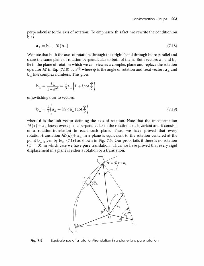
Transformation Groups 203
perpendicular to the axis of rotation. To emphasize this fact, we rewrite the condition onb as
a⊥ = b⊥ −R(b⊥) (7.18)
We note that both the axes of rotation, through the origin 0 and through b are parallel andshare the same plane of rotation perpendicular to both of them. Both vectors a⊥ and b⊥lie in the plane of rotation which we can view as a complex plane and replace the rotationoperatorR in Eq. (7.18) by eiφ where φ is the angle of rotation and treat vectors a⊥ andb⊥ like complex numbers. This gives
b⊥ =a⊥
1− eiφ=
12
a⊥
(1+ i cot
φ
2
)or, switching over to vectors,
b⊥ =12
(a⊥+ (n× a⊥)cot
φ
2
)(7.19)
where n is the unit vector defining the axis of rotation. Note that the transformationR(x) + a⊥ leaves every plane perpendicular to the rotation axis invariant and it consistsof a rotation-translation in each such plane. Thus, we have proved that everyrotation-translation R(x) + a⊥ in a plane is equivalent to the rotation centered at thepoint b⊥ given by Eq. (7.19) as shown in Fig. 7.5. Our proof fails if there is no rotation(φ = 0), in which case we have pure translation. Thus, we have proved that every rigiddisplacement in a plane is either a rotation or a translation.
Fig. 7.5 Equivalence of a rotation/translation in a plane to a pure rotation
204 An Introduction to Vectors, Vector Operators and Vector Analysis
It is immediate from Eq. (7.17) that b⊥ = 0 impliesRb =R . Thus, the rotations differingby the shift of origin along the rotation axis are equivalent. Indeed, no parameters definingthe rotation change by a translation along the axis of rotation.
7.3.1 Chasles theorem
Given any rigid displacement σ (x) = R(x) + a, we decompose the translation a intocomponents a‖ and a⊥, parallel and perpendicular to the rotation axis defined by R ,so that
σ (x) =R(x) + a⊥+ a‖ (7.20)
NowR(x) + a⊥ can be treated as a rotationRb, so that
σ (x) = τa‖Rb(x) (7.21)
where τa‖ is the translation parallel to the rotation axis Rb. Equation (7.21) provesChasles theorem: Any rigid displacement can be expressed as a screw displacement. Ascrew displacement consists of a product of rotation with a translation along the axis ofrotation (the screw axis). We have done more than proving Chasles theorem, we haveshown how to find the screw axis of a given rigid displacement. Although elegant, Chaslestheorem is seldom used in practice. Equation (7.11) is usually more useful, because thecenter of rotation (the origin) can be specified at will to simplify the problem at hand.Finally, note that b = b‖ (i.e., b⊥ = 0 in Eq. (7.16)) gives, via Eq. (7.12),
Rb(x) =R(x) (7.22)
as it should.
Exercise A rigid displacement σ (x) = R(x) + a can be expressed as a product of atranslation τc and a rotationRb centered at a specified point b. Determine the translationvector c.
Hint Using Eq. (7.12) R(x) + a = τcRb can be reduced to c = a − b +R(b). a,bmay be specified as column or row matrices andR ∈ SO(3) as a 3× 3 special orthogonalmatrix. OtherwiseR may be given as a rotation operator.
Exercise A subgroup H of group G is called an invariant subgroup if g−1hg ∈ H forevery h ∈ H and every g ∈ G. Show that the translations T form an invariant subgroup ofthe group E of isometries on E3.
Solution Let σ ∈ E and τa ∈ T . Then,
(σ−1τaσ )(x) = x+ σ−1(a)
which is a translation τσ−1(a) ∈ T .
Transformation Groups 205
Exercise Let S denote the reflection in the plane normal to a non-zero vector a. If τa isthe translation by a then Sa = τaSτ−a is the reflection S shifted to the point a. Show that
SS−a = τ2a.
Thus, a translation by a can be expressed as a product of reflections in parallel planesseparated by 1
2 a.
Solution Since S is a linear operator, S2 = I and S(a) = −a, we have,
S−a(x) = S(x+ a)− a = S(x) + S(a)− a
= S(x)− 2a
giving
SS−a = S2(x)− 2S(a) = x+ 2a = τ2a.
7.4 Similarities and CollineationsIsometries preserve lengths of vectors as well as the angles between vectors. We call a non-empty subset of E3 a figure. Two figures S and S∗ in E3 are congruent if and only if S∗ =σ (S) for some isometry σ on E3.
Exercise Show that congruence is an equivalence relation.
Solution This is obvious because isometries form a group.
(i) Since identity is an isometry, a figure is congruent to itself.(ii) S∗ = σ (S) implies S = σ−1S∗ so that congruence is reflexive.
(iii) Since a composition of isometries is an isometry, if S1 is congruent to S2 and S2 iscongruent to S3 then S1 is congruent to S3. Thus, congruence is transitive.
Two figures are said to be similar if they have the same shape but not the same size, so thatone is congruent to an enlargement of the other. Two figures S and S∗ are similar if andonly if S∗ = Σ(S) where Σ, is called a similarity transformation on E3, and is given by
Σ : x 7→ λA(x) + a, λ ∈R, λ , 0,A orthogonal
If λ < 0 then we take −A to be the orthogonal transformation. Similarity transformationsform a group which contains isometries as a subgroup. The similarity transformations donot preserve distance however, they preserve ratios of distances, that is,
d(Σ(a),Σ(b))d(Σ(c),Σ(d))
=d(a,b)d(c,d)
·
206 An Introduction to Vectors, Vector Operators and Vector Analysis
Both isometries and similarities are subgroups of a more general group of transformationscalled collineations which transform lines into lines. All transformations of the form
A : x 7→ A(x) + a A invertible
are collineations and are called Affine transformations. Affine transformations form agroup called Affine group. Note that both isometries and similarities are affinetransformations.
Let G be the affine group and let Ω be the set which is either E3 or a class of figuresin E3 but not both. We define a relation ≡ on Ω namely, α ≡ β if and only if there existsσ ∈ G such that σ (α) = β.
Exercise Show that ≡ is an equivalence relation.
Hint Again, this follows from the fact that affine transformations form a group. Soproceed just the way we showed congruence to be an equivalence relation.
Consider a subset of Ω consisting of all elements which are related via ≡. Such a subset iscalled an equivalence class of ≡. To construct such a subset pick up an element in Ω andcollect all elements of Ω related to it. If the complement of this subset in Ω is not empty,pick out an element from the complement and collect all elements related to it. Repeat thisprocedure until all of Ω is exhausted. Obviously, all these subsets, or equivalence classes,are mutually exclusive, because if any two of them have an element in common, bytransitivity property it will be related to all the elements of both the subsets, so that theirunion will form a single equivalence class. Thus, Ω is partitioned by its equivalenceclasses, that is, two equivalence classes have empty intersection and the union of all ofthem is Ω.
When G is the affine group the elements of the equivalence class of ≡ on Ω via G arecalled affine equivalent.
Instead of defining via the affine group, we can define ≡ via the similarity group or theisometry group to get the same results.
We now classify the set of all central conics, (defined below), which are the orbits ofparticles driven by the inverse-square law of force, using group of affine transformations orgroups of isometries and similarities.
Conics are the loci of the second degree, that is, the non-empty point sets in E2, givenby Sprienger
Γ = (x,y)|ax2 + 2hxy+ by2 + 2gx+ 2f y+ c = 0 a , 0 or h , 0 or b , 0
Conics for which ab , h2 are called central conics.We intend to examine the effect of an affine (or isometry or similarity) transformation
on a conic Γ . The equation of Γ , mentioned in its definition can be alternatively expressedin the matrix form as
uAuT + 2ukT + c = 0 (7.23)
Transformation Groups 207
where u,k are 1× 2 matrices and a is a 2× 2 symmetric matrix
u =(x y
)A=
(a h
h b
)k =
(g f
)and c is a 1 × 1 matrix. Now we make an affine transformation σ : u 7→ u′ = [x′,y′] sothat u = u′S +w (S invertible) and obtain the matrix equation
(u′S +w)A(ST (u′)T +wT ) + 2(u′S +w)kT + c = 0
which can be simplified to
u′A′(u′)T + 2u′(k′)T + c′ = 0 (7.24)
where A′ = SAST , k′ = kST +wAST and c′ = c+ 2wkT +wAwT . Equation (7.24) isagain a second degree equation so that (x′,y′) must lie on a conic
Γ ′ = (x,y) | a′x2+2h′xy+b′y2+2g ′x+2f ′y+c′ = 0 a′ , 0 or h′ , 0 or b′ , 0
Since det A′ = (det S)2 det A (det S , 0) we have ab , h2 if and only if a′b′ , (h′)2 ; inother words, central conics are transformed into central conics. Now choose thetransformation w = −kA−1 giving k′ = 0, thus eliminating all the first degree terms fromEq. (7.24). The point represented by the vector −kA−1 is called the center of the conic Γ .Note that when ab = h2, A−1 does not exists and Γ cannot have a center. Usingw = −kA−1 we obtain c′ = c − kA−1kT which on evaluation gives
c′ =∆
ab − h2
∆ = abc+ 2f gh− af 2 − bg2 − ch2 (7.25)
To find the affine equivalent class of central conics, we have to find the criteria whichguarantee (or otherwise) the existence of an affine transformation connecting the givenconics Γ and Γ ′ . That is, given Γ and Γ ′, as in Eqs (7.23) and (7.24), when can one find aninvertible matrix S transforming Γ ′ to Γ . We differ this question until we have obtainedthe effect of the Euclidean transformations (isometries) on central conics and find itsequivalence classes.
When σ : u 7→ u′ is an isometry, the above analysis goes through, with the reservationthat the matrix S defined by u = u′S +w must be orthogonal. We are interested in theisometries continuously connected to identity, so we restrict to the Euclidean group andrequire S to be special orthogonal (det S = +1). Since A is symmetric and S is specialorthogonal, we can choose S such that the matrixA′ = SAST is diagonal with the diagonalelements as the eigenvalues of A. Thus, we can write A′ = diag(λ,µ) where λ,µ are the
208 An Introduction to Vectors, Vector Operators and Vector Analysis
roots of the equation t2 − (a + b)t + ab − h2 = 0. We can therefore find an Euclideantransformation which takes the central conic Γ into the conic Γ ′ with equation
λx2 + µy2 +∆/(ab − h2) = 0 (7.26)
If ∆ , 0 Eq. (7.26) can be rewritten as
αx2 + βy2 = 1 (7.27)
where α+ β = −(a+ b)(ab − h2)/∆, αβ = (ab − h2)3/∆2.We will now show that the pair of numbers α,β characterizes the Euclidean
equivalence class of Γ . If Γ is Euclidean equivalent to a conic Γ ′′ with the equation
γx2 + δy2 = 1 (7.28)
then there is a transformation [x y] 7→ [x y]U + c (U orthogonal) taking Γ ′ to Γ ′′. It iseasily seen that we must have c = 0 and(
γ 00 δ
)= U
(α 00 β
)UT
which is possible if and only if γ ,δ = α,β. Thus, two central non-degenerate (i.e.,∆ , 0) conics are Euclidean equivalent if and only if they have the same values for α and βor, equivalently, for α+ β and αβ given by Eq. (7.27). In other words, the quantities
−(a+ b)(ab − h2)
∆and
(ab−h2)3
∆2 (7.29)
are invariants for the central (ab , h2) and non-degenerate (∆ , 0) conics under the actionof the Euclidean group.
Under the similarity group, any central non-degenerate conic again reduces to a conicwith Eq. (7.27), but this conic is equivalent to the conic in Eq. (7.28) if and only if eitherγ/δ = α/β or γ/δ = β/α. The pair α/β,β/α or equivalently the number (α/β) +(β/α) or equivalently the number
(α+ β)2
αβ=
(a+ b)2
(ab − h2)(7.30)
is the required invariant under the similarity group.Under the affine group, the conics with Eqs (7.27) and (7.28) are equivalent if and only
if αβ and γδ have the same sign, because in this case (with U an invertible matrix notnecessarily orthogonal) the determinants of the corresponding matrices are related by
γδ = (det U )2αβ (7.31)
Transformation Groups 209
and since the conic is central, αβ , 0. We also note that both α and β cannot be < 0because in that case, no (x,y) can satisfy Eq. (7.27). Thus, Eq. (7.31) does imply that αβand γδ have the same sign. There are thus only two affine equivalent classes of centralnon-degenerate conics, namely those for which ab − h2 > 0 (ellipses) and those for whichab − h2 < 0 (hyperbolae). Note that in the affine geometry, any two ellipses are equivalent,while in Euclidean geometry they are equivalent if they have the same pair of Euclideaninvariants given by Eq. (7.29), which means that the two ellipses must be of the same size.
All ellipses are affine equivalent to the locus of the equation x2+y2 = 1 that is the unitcircle. All hyperbolae are affine equivalent to the locus of the equation x2 − y2 = 1. This isa disconnected set with two components, namely,
(x,y) | x2 − y2 = 1, x > 0 and (x,y) | x2 − y2 = 1, x < 0.
Finally, we note that the Euclidean equivalent figures have the following property: Onefigure can be superposed on the other by rigid displacement. Thus, the group of rigiddisplacements describes all possible relations of congruency. These relations underlie allphysical measurements. A ruler is a rigid body and any measurement of length involvesrigid displacements to compare a ruler with the object being measured.
Exercise This is a small project for the students:
Discuss the Euclidean, similarity and affine equivalence classes of non-singular centralquadrics in E3 i.e., the loci
(x,y,z) | ax2 + by2 + cz2 + 2f yz+ 2gzx+ 2hxy+ 2ux+ 2vy+ 2wz+ d = 0
with ∣∣∣∣∣∣∣∣∣a h g
h b f
g f c
∣∣∣∣∣∣∣∣∣ , 0
∣∣∣∣∣∣∣∣∣∣∣∣a h g u
h b f v
g f c w
u v w d
∣∣∣∣∣∣∣∣∣∣∣∣, 0,
where vertical bars mean the determinants of the corresponding matrices. Show inparticular, that there are three affine equivalent classes and find simple canonicalrepresentatives of these classes.

Part III
Vector Analysis

Transformation Groups 213
This may be translated as follows:1Multiply the arc by the square of the arc and take the result of repeating that [any
number of times]. Divide [each of the above numetrators] by the squares of successiveeven numbers increased by that number [lit. the root] and multiplied by the square of theradius. Place the arc and the successive results so obtained one below the other andsubtract each from the one above. These together give the Jiva, as collected together in theverse beginning with “vidvan” etc.
Indian mathematics and astronomy dealt not directly with present-day sines andcosines but with these quantities multiplied by the radius r of a standard circle. Thus, jivacorresponds to r sinθ while sara corresponds to r(1− cosθ).
In the present-day mathematical terminology the above passage says the following. Letr denote the radius of the circle, s denote the arc and tn the nth expression obtained byapplying the rule cited above. The rule requires us to calculate as follows.
1. Numerator: Multiply the arc s by its square s2, this multiplication being repeated ntimes to obtain s ·Πn
1s2.
2. Denominator: Multiply the square of the radius, r2, by [(2k)2 + 2k] (“squares ofsuccessive even numbers increased by that number”) for successive values of k,repeating this product n times to obtain Πn
k=1r2[(2k)2 + 2k].
Thus, the nth iterate is obtained by
tn =s2n · s
(22 + 2) · (42 + 4) · · · [(2n)2 + 2n] · r2n
The rule further says:
jiva = s − t1 + t2 − t3 + t4 − t5 + · · ·
= s − s3
r2 · (22 + 2)+
s5
r4(22 + 2)(42 + 4)− · · ·
1This epighraph is taken from ref.[18]
214 An Introduction to Vectors, Vector Operators and Vector Analysis
Substituting
(i) jiva= r sinθ,
(ii) s = rθ, so that s2n+1/r2n = rθ2n+1 and noticing that(iii) [(2k)2 + 2k] = 2k · (2k+ 1) so that(iv) (22 + 2) · (42 + 4) · · · [(2n)2 + 2n] = (2n+ 1)!,
and cancelling r from both sides, we see that the infinite series for Jiva is entirely equivalentto the well known Taylor series for sinθ :
sinθ = θ − θ3
3!+θ5
5!− θ
7
7!+ · · ·
It is now well known that calculus was developed in India starting mid-fifth century(Aryabhata in Bihar) until mid-fourteenth century (Madhava in Kerala) with a long list ofbrilliant mathematicians filling in the gap. Indians invented powerful techniques toaccelerate convergence of a series and to sum a given series to the required accuracy [18].Thus, Madhava produced a table of values of sinθ and cosθ exact upto ten decimal digitsby summing up their Taylor series (better called Madhava series!). Values to this accuracywere required for navigation (locating ships and finding directions on open sea) andtimekeeping (yearly scheduling of agricultural activities, vis-a-vis rainy season, tomaximize production).
8
Preliminaries
8.1 Fundamental NotionsThis part deals with the basic concepts and applications of differential and integral calculusto functions involving vector variables. By a function we mean a one to one or many to onemapping between non-empty sets say X and Y and denote it by f : X 7→ Y . In general, fmaps a subset of X, called its domain and denoted D(f ), to a subset of Y called its rangeor image set and denoted R(f ). If R(f ) = Y then the function is called onto. If f isone to one and onto, it is invertible (see section 4.1). Note that the sets X and Y can beidentical, X = Y , so that the function is f : X 7→ X and both the domain and the rangeof f are the subsets of the same set X. If x ∈ D(f ) is mapped to y ∈ R(f ) under f , thenx is called the argument of f , y is called the image of x under f and is denoted f (x), thatis, y = f (x). f (x) is said to be the value of the function f at x. In general, we can say thatx is a variable taking values in D(f ) and f (x) are the corresponding values inR(f ). Theimage set of a subset E ⊆ D(f ) under f is denoted f (E). The equality, addition as well asthe composition of two or more functions is exactly as given in section 4.1.
In this book we are concerned with the following three classes of functions.
• Vector valued functions of a scalar variable f : R 7→ E3. These functions generallyoccur as a part of the kinematics and dynamics of a physical system. For example, thevelocity of a particle as a function of time v(t).
• Scalar valued functions of a vector variable, f : E3 7→R. All scalar fields φ(x) fall inthis category, as a scalar field is a scalar valued function of position vectors or pointsin space, e.g., the temperature profile in a region of space.
• Vector valued functions of a vector variable, f : E3 7→ E3. All linear operators on E3fall in this category. All vector fields are also functions (of position vectors) falling inthis class.
In what follows we assume that the space E3 or (R3) and a real line R form a continuum(see section 1.2). We also treat these as metric spaces with Euclidean metric.
216 An Introduction to Vectors, Vector Operators and Vector Analysis
In this chapter, a vector is referred to either as a vector or as a point in space. Further,in this chapter we use the same symbol to indicate a vector or a scalar, because whateveris said about it applies to both the cases. At any rate, its being a vector or a scalar can beunderstood with reference to context. Also, by a function we mean a function in one of thethree categories described above.
8.2 Sets and MappingsWe need the following properties of sets and mappings all shared by the subsets of E3and R.
Two sets A and B are said to be in 1 − 1 correspondence if a one to one and onto mapcan be found between them. Such sets are said to have the same cardinality or are said tobe equivalent and we write A ∼ B. Clearly, the relation A ∼ B has the following properties.
• Reflexivity: A ∼ A.
• Symmetry: If A ∼ B then B ∼ A.
• Transitivity: If A ∼ B and B ∼ C then A ∼ C.
Exercise Prove the above properties.
Hint The identity I : A 7→ A is a 1−1 correspondence. Inverse of a 1−1 correspondence isa 1−1 correspondence. Composition of two 1−1 correspondences is a 1−1 correspondence.
Let Nk denote the set 1,2, . . . ,k for some integer k > 0 and let N be the set 1,2,3, . . . ofall integers > 0. Given a set A we say
• A is finite if A ∼Nk for some k ≥ 0. The empty set corresponding to k = 0 is alsoconsidered to be finite.
• A is infinite if it is not finite.• A is countable if A ∼N.
• A is uncountable if it is neither finite nor countable.
A countable set is sometimes called enumerable or denumerable.For two finite sets A and B we evidently have A ∼ B if and only if they contain the same
number of elements. The set I of all integers is countable as can be seen from the following1− 1 correspondence between I and N.
I : 0 1 − 1 2 − 2 3 − 3 · · ·
N : 1 2 3 4 5 6 7 · · ·
Exercise Find f : N 7→ I generating this 1− 1 correspondence.
Preliminaries 217
Answer
f (n) =
n2 (n even)
−n−12 (n odd).
This example shows that an infinite set can be put to 1− 1 correspondence with one of itsproper subsets. This is not possible for finite sets.
Since R, R3 and E3 are continua, we expect each of them to form an uncountable set.Also, every subset of these spaces, which forms a continuous region of space must also bean uncountable set. We accept this to be true without supplying any proofs.
8.3 Convergence of a SequenceAll analysis, be it real, complex or vector analysis, can be constructed on the basis of asingle fundamental concept, namely, the convergence of an infinite sequence of points (orsequence for short) in the given space.
A sequence is a function defined on the set of all positive integers 1,2,3, . . .. We arebasically interested in sequences defined by the functions f : N 7→ R and f : N 7→ E3which are the sequences of scalars and vectors respectively. We denote the sequence f (n) =xn, (n ∈N) by the symbol xn or by x1,x2,x3, . . . . The elements xn forming the sequenceare called the terms of the sequence. IfA is a set and if xn ∈ A for all n ∈N then xn is saidto be a sequence in A. Note that the terms of a sequence may be distinct or identical. Theset of all points xn, (n= 1,2, . . .) is the range of the sequence xn. The range of a sequencemay be a finite set or it may be infinite. A sequence xn is said to be bounded if its rangeis bounded (that is, the set formed by the distinct elements of a sequence is a bounded set,see below). We are interested in sequences in R or in E3.
The concept of the convergence of a sequence in a metric space can be defined withoutreferring to a particular metric space. Therefore, we define the the convergence of asequence in a metric space X which stands for both R and E3. A subset S ⊂ X is said to bebounded if there is a real M > 0 satisfying d(p,q) ≤ M for all p,q ∈ S. The smallest Msatisfying this condition is called the diameter of S. A r-neighborhood of a point p ∈ X isa set Nr(p) consisting of all points q such that d(p,q) < r. The number r is called theradius of Nr(p). An open set is a subset E of X such that every point in it has aneighborhood which is a proper subset of that set. Each such point is called an interiorpoint so an open set is the one whose every element is an interior point. In particular, ar-neighborhood of any point in a metric space is an open set. A point p ∈ E is itsboundary point if every neighborhood of p has a point q ∈ E, q , p, but is not a subset ofE. A set containing all its interior as well as its boundary points is called a closed set. Thus,the set of all points inside a sphere of radius R is an open set while the points on the sphereform the set of boundary points. In general, in a metric space, given ε > 0, the set of pointswith distance < ε from a given point form the ε-neighborhood of that point. The set ofpoints at a distance ε from the given point form the set of boundary points of thisε-neighborhood.
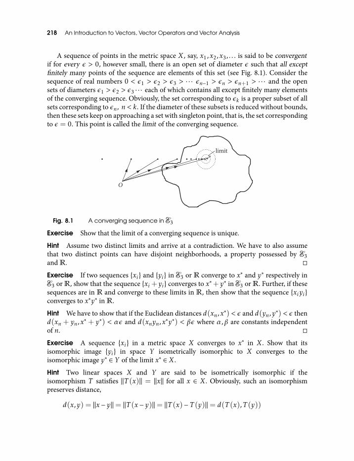
218 An Introduction to Vectors, Vector Operators and Vector Analysis
A sequence of points in the metric space X, say, x1,x2,x3, . . . is said to be convergentif for every ε > 0, however small, there is an open set of diameter ε such that all exceptfinitely many points of the sequence are elements of this set (see Fig. 8.1). Consider thesequence of real numbers 0 < ε1 > ε2 > ε3 > · · · εn−1 > εn > εn+1 > · · · and the opensets of diameters ε1 > ε2 > ε3 · · · each of which contains all except finitely many elementsof the converging sequence. Obviously, the set corresponding to εk is a proper subset of allsets corresponding to εn, n < k. If the diameter of these subsets is reduced without bounds,then these sets keep on approaching a set with singleton point, that is, the set correspondingto ε = 0. This point is called the limit of the converging sequence.
Fig. 8.1 A converging sequence in E3
Exercise Show that the limit of a converging sequence is unique.
Hint Assume two distinct limits and arrive at a contradiction. We have to also assumethat two distinct points can have disjoint neighborhoods, a property possessed by E3and R.
Exercise If two sequences xi and yi in E3 or R converge to x∗ and y∗ respectively inE3 or R, show that the sequence xi+ yi converges to x∗+ y∗ in E3 or R. Further, if thesesequences are in R and converge to these limits in R, then show that the sequence xiyiconverges to x∗y∗ in R.
Hint We have to show that if the Euclidean distances d(xn,x∗) < ε and d(yn,y∗) < ε thend(xn + yn,x∗ + y∗) < αε and d(xnyn,x∗y∗) < βε where α,β are constants independentof n.
Exercise A sequence xi in a metric space X converges to x∗ in X. Show that itsisomorphic image yi in space Y isometrically isomorphic to X converges to theisomorphic image y∗ ∈ Y of the limit x∗ ∈ X.
Hint Two linear spaces X and Y are said to be isometrically isomorphic if theisomorphism T satisfies ||T (x)|| = ||x|| for all x ∈ X. Obviously, such an isomorphismpreserves distance,
d(x,y) = ||x − y||= ||T (x − y)||= ||T (x)− T (y)||= d(T (x),T (y))
Preliminaries 219
from which the result follows. Thus, a sequence in E3 converging to a vector in E3 is also asequence in R3 converging to a point represented by the vector at the limit.
Uniqueness of the limit of a converging sequence enables us to re-define its convergence asfollows.
A sequence xi in a metric space X is a sequence converging to x∗ if for every ε > 0there is an integer n0 > 0 such that d(xn,x∗) < ε whenever n > n0. The fact that x∗ is thelimit of a converging sequence xk is summarily expressed as limk→∞ xk = x∗.
Exercise Suppose xn is in R and limn→∞ xn = x∗. Show that limn→∞1xn
= 1x∗
provided xn , 0, (n= 1,2, . . .) and x∗ , 0.
Exercise
(a) Suppose xn ∈ R3(n = 1,2,3, . . .) and xn = (α1,n,α2,n,α3,n). Then xn converges tox = (α1,α2,α3) if and only if limn→∞αj,n = αj , j = 1,2,3.
(b) Suppose xn yn are sequences in R3 and βn is a sequence in (R) and xn → x,yn→ y, βn→ β. Then,
limn→∞
(xn+ yn) = x+ y limn→∞
(xn · yn) = x · y limn→∞
βnxn = βx.
Solution
(a) If xn→ x, the inequalities
|αj,n −αj | ≤ |xn − x|
which follow immediately from the definition of the norm in R3 show thatlimn→∞αj,n = αj , j = 1,2,3.
Conversely, if limn→∞αj,n = αj , j = 1,2,3, then to each ε > 0 there is an integerN such that n ≥N implies
|αj,n −αj | <ε√
3j = 1,2,3.
Hence, n ≥N implies
|xn − x|=
3∑j=1
|αj,n −αj |2
12
< ε,
so that xn→ x, which proves (a).
(b) Hint Use part (a).
220 An Introduction to Vectors, Vector Operators and Vector Analysis
8.4 Continuous FunctionsConsider a converging sequence x1,x2,x3, . . . in the domain D(f ) of a function f with itslimit x∗ ∈ D(f ). The function f is said to be continuous at x∗ if the sequencef (x1),f (x2),f (x3), . . . converges to the limit f (x∗) and this happens for all sequences inD(f ) converging to x∗. The continuity of a function at a point can be expressed as
limx→x∗
f (x) = f (x∗),
or,
limx→x∗
d(f (x),f (x∗)) = 0,
or, assuming the Euclidian distance
limx→x∗||f (x)− f (x∗)||= 0.
Exercise Show that if the functions f (x) and g(x) are continuous at x∗ then so is theirsum f (x) + g(x) and their product f (x)g(x).
In general, we say that
limx→x∗
f (x)
exists if for every sequence xn converging to x∗, the corresponding sequence f (xn)converges to the same limit. In terms of this definition, the result of the third exercise ofthis section can be used to get
limx→x∗
[f (x) + g(x)] = limx→x∗
f (x) + limx→x∗
g(x) (8.1)
and
limx→x∗
[f (x)g(x)] = [ limx→x∗
f (x)][ limx→x∗
g(x)]. (8.2)
provided the limits on the RHS of these equations exist.
9
Vector Valued Functions ofa Scalar Variable
We start with the functions in the first of the three categories described above, namely, thevector valued functions of a scalar variable, denoted f(t).
9.1 Continuity and Differentiation
The derivative of f(t) with respect to the scalar variable t is a new function denoted df(t)dt
or f(t) and is defined by
f(t) =df(t)dt
= lim∆t→0
f(t+∆t)− f(t)∆t
. (9.1)
This limit, when evaluated at a particular value t = t0, gives the value of the derivative off(t) at t0, that is, the value of f(t0) or df
dt (t0). We say that the function f(t) is differentiableat t0 if this limit exists at t = t0.
Note that, to be differentiable at t0, f(t) must be continuous at t0, that is,
lim∆t→0
f(t0 +∆t) = f(t0)
Otherwise, the RHS of Eq. (9.1) will blow up as ∆t → 0 because the numerator remainsfinite while the denominator tends to zero.
The derivative f(t) is a function of t in its own right, therefore we can differentiate itby applying Eq. (9.1) to it, provided the corresponding limit exists. The resulting derivativefunction is called the second derivative of f(t) and is denoted f(t) or d2f
dt2(t). Continuing
in this way we can define the third and higher order derivatives of f(t).As an important application, we consider a particle moving along a path which is a
continuous and differentiable curve, that is, the curve is the graph of a continuous and
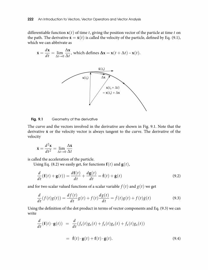
222 An Introduction to Vectors, Vector Operators and Vector Analysis
differentiable function x(t) of time t, giving the position vector of the particle at time t onthe path. The derivative x = x(t) is called the velocity of the particle, defined by Eq. (9.1),which we can abbrivate as
x =dxdt
= lim∆t→0
∆x∆t
, which defines ∆x = x(t+∆t)− x(t).
Fig. 9.1 Geometry of the derivative
The curve and the vectors involved in the derivative are shown in Fig. 9.1. Note that thederivative x or the velocity vector is always tangent to the curve. The derivative of thevelocity
x =d2xdt2
= lim∆t→0
∆x∆t
is called the acceleration of the particle.Using Eq. (8.2) we easily get, for functions f(t) and g(t),
ddt
(f(t) + g(t)) =df(t)dt
+dg(t)dt
= f(t) + g(t) (9.2)
and for two scalar valued functions of a scalar variable f (t) and g(t) we get
ddt
(f (t)g(t)) =df (t)
dtg(t) + f (t)
dg(t)
dt= f (t)g(t) + f (t)g(t) (9.3)
Using the definition of the dot product in terms of vector components and Eq. (9.3) we canwrite
ddt
(f(t) · g(t)) =ddt
(fx(t)gx(t) + fx(t)gx(t) + fx(t)gx(t))
= f(t) · g(t) + f(t) · g(t). (9.4)
Vector Valued Functions of a Scalar Variable 223
In particular, for a particle with velocity v(t) and speed function v(t) = |v(t)| we get
ddtv2(t) =
ddt
(v(t) · v(t)) = 2v(t) · v(t).
This equation relates the rate of change of kinetic energy of a particle with its velocity andacceleration. On the other hand, if the particle is moving along a straight line, so that itsdirection v is constant while its speed changes with time, (v(t) = v(t)v), then,
ddtv2 = 2vv = 2vvv · v = 2v · v.
We shall now show that a vector valued function v(t) has constant magnitude if and onlyif there is a vector ω satisfying
v = ω × v (9.5)
To show that Eq. (9.5) implies constant magnitude for v, we just dot both sides by v to getv ·ω × v on RHS which is zero. This means 2v · v = d
dtv2 = 0 or |v| is constant.
To show that constant magnitude of v, that is, 2v · v = ddtv
2 = 0 implies the existenceof someω satisfying Eq. (9.5), we chooseω = (v× v)/v. Using identity I and the fact thatv · v = 0 we can easily check that this ω satisfies Eq. (9.5).
Exercise If n is a unit vector function of the scalar variable t, then show that∣∣∣∣∣n× dndt
∣∣∣∣∣= ∣∣∣∣∣dndt
∣∣∣∣∣ .Solution We make use of the fact that the vector of constant magnitude is perpendicularto its derivative. Thus, n is perpendicular to dn
dt . Therefore, we have,∣∣∣∣∣n× dndt
∣∣∣∣∣= |n| ∣∣∣∣∣dndt
∣∣∣∣∣sinπ2=
∣∣∣∣∣dndt
∣∣∣∣∣since |n|= 1.
Exercise Let u = u(t) be a vector valued function and write u = |u|. Show that
ddt
(u(t)) =ddt
(uu
)=
(u× u)×uu3 .
Solution By straightforward differentiation we get
ddt
(uu
)=uu− uuu2 .
224 An Introduction to Vectors, Vector Operators and Vector Analysis
Now consider
(u× u)×uu3 =
u2u− (u · u)uu3 =
uu− uuu2
where the last equality follows from u · u = 12ddtu
2 = uu.
Exercise Show that the conservation of angular momentum (h) of a particle driven by acentral force, (h = 0), implies that both the magnitude and the direction of h are conservedseparately. Use this to show that the orbit of the earth around the sun never changes thedirection of its circulation about the sun.
Solution To prove the first part consider h = 0 implies h · h = 0 which impliesddt (h ·h) =
ddt (h
2) = 0, where h = |h|. Thus, the magnitude of h is conserved separately.Now, h = constant and hh = constant together imply h = constant so that the directionof h is separately conserved.
To get the second part, note that, for constant magnitude of h,
0 ≤ |h|= h=mr2θ, (9.6)
where r is the distance of the particle from the center of force. Equation (9.6) implies thatθ ≥ 0 always, in a dextral (that is, right handed) frame so θ = θ(t) increasesmonotonically with time if h , 0. In a left handed frame θ ≤ 0. What is important (andphysical) is that θ cannot ever change its sign. This means that the orbit of the earth in thecentral force field of the sun never changes the direction of its circulation, as the angularmomentum of its orbital motion around the sun is conserved. Note that this result appliesto all central forces.
Let us now see the effect of differentiation on the vector product of two functions andthe product of a vector valued and the scalar valued function. Let A(t) and B(t) be twovector valued functions of a scalar variable t and φ(t) be a scalar valued function of t.Differentiating (A(t)×B(t))i = εijkAj(t)Bk(t) we get,
ddt
(A(t)×B(t)) =dAdt×B+A× dB
dt. (9.7)
Also, by differentiating the product of functions we get,
ddt
(φA) =dφ
dtA+φ
dAdt
. (9.8)
We can summarily conclude
• If dAdt ·A = 0 then |A| is constant.
• If A× dAdt = 0, A , 0, then dA
dt is parallel to A implying that A has constant direction.
Vector Valued Functions of a Scalar Variable 225
9.2 Geometry and Kinematics: Space Curves and Frenet–SeretFormulae
Frenet–Seret formulae help us connect the geometry of the path of a particle with itskinematics. We have seen that a path of a particle, which we assume to be a smooth curvegiven by a continuous and differentiable function x(t), is parameterized by time t. That is,evaluation of x(t) at some value of the scalar parameter t, say x(t0) at t = t0, correspondsto a unique point on the path giving the position of the particle at time t = t0. The vectorvalued function x(t) is equivalent to the triplet of scalar valued ‘coordinate functions’(x(t),y(t),z(t)) which are the components of x(t) with respect to some orthonormalbasis.
For a curve C, the function x(t) ≡ (x(t),y(t),z(t)) above, defines a one to one map ofthe t-axis onto the curve, that is, a point on the t-axis is mapped to the unique point x(t) ≡(x(t),y(t),z(t)) on the curve C. Since the function x(t) ≡ (x(t),y(t),z(t)) is assumedcontinuous, neighboring points on the t-axis correspond to the neighboring points on thecurve. Since the points on the t-axis are ordered, we can assign an order or the ‘sense’ tothe points of C by saying that the point x(t1) on C precedes point x(t2) on C if t1 < t2.The parametric representation thus gives a precise meaning to the sense in which a curveis traversed, using the order of points on a line. This still allows for the possibility x(t1) =x(t2) on C even if t1 , t2 which just means that the particle was at the same point on thecurve at two different times t1 and t2. This is possible if path is a simple closed curve or hasa loop. A point on the curve at which dx
dt , 0 is called a regular point.The same path can be parameterized by different parameters, given by different
monotonic functions of t. For example, a circle can be parameterized by angle θ made bythe radius vector with the positive direction of the x axis say θ = ωt where ω is theangular or rotational velocity of the particle along the circle. Another possibleparameterization is by arc length. This parameter is given by the distance s(t) traversed bythe particle along the path, measured from a fixed point on the path which corresponds tot = 0. The path then becomes the graph of the function x(s). The value x(s0) at s = s0simply gives the position vector of the particle at a point on the path, reached bytraversing the path of length s0 from the chosen fixed point on the path. While measurings0 the path is traversed in the same sense in which the moving particle traverses the path,with increasing time, as we saw in the above paragraph. All this is depicted in Fig. 9.2.
Mathematically, we change the parameter from arc length s to time t, in the range s1 ≤s ≤ s2, by means of an analytic function s = s(t) with s1 = s(t1) and s2 = s(t2) such thatdsdt > 0 in t1 ≤ t ≤ t2. This ensures that the inverse function t(s) exists and is analytic ins1 ≤ s ≤ s2 and that dtds > 0 there. This ensures 1-1 correspondence between the values ofs and t in their domains and both parameterizations traverse the curve in the same senseas they increase through their values. As dx
dt = dxdsdsdt and ds
dt , 0 a regular point for theparameter s is also the regular point for the parameter t.
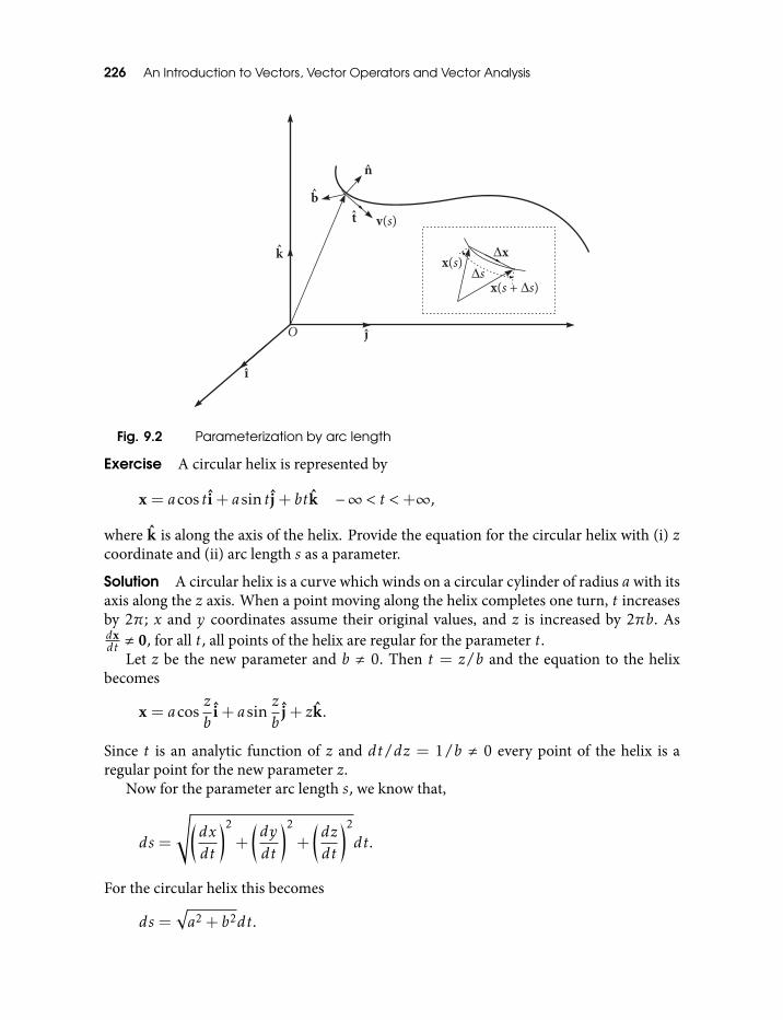
226 An Introduction to Vectors, Vector Operators and Vector Analysis
Fig. 9.2 Parameterization by arc length
Exercise A circular helix is represented by
x = acos ti+ asin tj+ btk −∞ < t <+∞,
where k is along the axis of the helix. Provide the equation for the circular helix with (i) zcoordinate and (ii) arc length s as a parameter.
Solution A circular helix is a curve which winds on a circular cylinder of radius a with itsaxis along the z axis. When a point moving along the helix completes one turn, t increasesby 2π; x and y coordinates assume their original values, and z is increased by 2πb. Asdxdt , 0, for all t, all points of the helix are regular for the parameter t.
Let z be the new parameter and b , 0. Then t = z/b and the equation to the helixbecomes
x = acoszb
i+ asinzb
j+ zk.
Since t is an analytic function of z and dt/dz = 1/b , 0 every point of the helix is aregular point for the new parameter z.
Now for the parameter arc length s, we know that,
ds =
√(dxdt
)2
+
(dy
dt
)2
+
(dzdt
)2
dt.
For the circular helix this becomes
ds =√a2 + b2dt.
Vector Valued Functions of a Scalar Variable 227
We choose s = 0 at t = 0 and integrate to get,
s = t√a2 + b2.
Therefore, in terms of s we get,
x = acoss
√a2 + b2
i+ asins
√a2 + b2
j+ bs
√a2 + b2
k.
Since dt/ds , 0, every point on the helix is regular with respect to parameter s.
Consider a point x(s0) on the path corresponding to s = s0. Let x + ∆x be the positionvector of a neighboring point corresponding to the parametric value s + ∆s. Since thecurve is smooth and x(s) is differentiable, there is a small enough neighborhood of x(s0)such that we can take |∆x| = |∆s|, that is, we can take the Euclidean distance betweenx(s0) and x(s0 + ∆s) to be the same as the distance traversed along the path betweenthese points. In the limit,
lim∆s→0
x(s0 +∆s)− x(s)∆s
=
[dxds
]s=s0
then becomes a unit vector tangential to the path at the point x(s0) pointing along thedirection given by the increasing values of s. Denoting this tangential unit vector by t wecan write
t =dxds
.
Since t is a unit vector we have t · t = 1 which gives
d tds· t = 0
that is, the vector d tds is orthogonal to t. This vector measures the amount by which the
direction of t changes as s increases i.e., as the particle moves along the path. We write
d tds
=
∣∣∣∣∣d tds
∣∣∣∣∣ n = κn (9.9)
where n is the unit vector in the direction of d tds and κ =
∣∣∣∣ d tds
∣∣∣∣ is the rate of change ofdirection of t with s. κ is called the curvature of the path at the point x(s0). n is called theprincipal normal unit vector. Note that n is always in the direction of d t
ds as κ is chosen tobe non-negative.
The equation κ = 1ρ defines the radius of curvature ρ at the corresponding point. A
straight line is a curve with zero curvature and infinite radius of curvature. In this case tis along the line and n can be in any direction perpendicular to t. The vector X = x + ρn
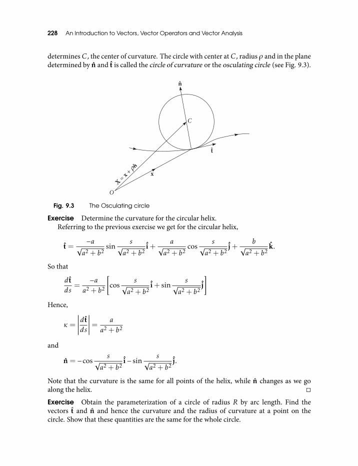
228 An Introduction to Vectors, Vector Operators and Vector Analysis
determinesC, the center of curvature. The circle with center atC, radius ρ and in the planedetermined by n and t is called the circle of curvature or the osculating circle (see Fig. 9.3).
Fig. 9.3 The Osculating circle
Exercise Determine the curvature for the circular helix.Referring to the previous exercise we get for the circular helix,
t =−a
√a2 + b2
sins
√a2 + b2
i+a
√a2 + b2
coss
√a2 + b2
j+b
√a2 + b2
k.
So that
d tds
=−a
a2 + b2
[cos
s√a2 + b2
i+ sins
√a2 + b2
j]
Hence,
κ =
∣∣∣∣∣∣d tds
∣∣∣∣∣∣= a
a2 + b2
and
n = −coss
√a2 + b2
i− sins
√a2 + b2
j.
Note that the curvature is the same for all points of the helix, while n changes as we goalong the helix.
Exercise Obtain the parameterization of a circle of radius R by arc length. Find thevectors t and n and hence the curvature and the radius of curvature at a point on thecircle. Show that these quantities are the same for the whole circle.
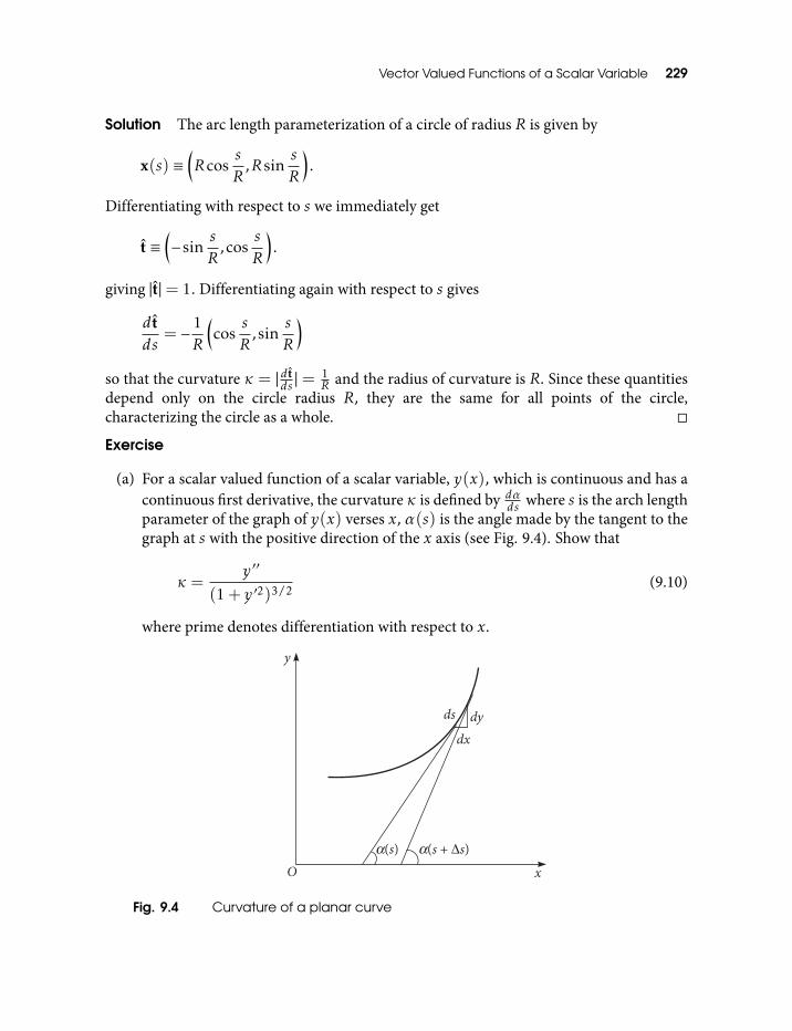
Vector Valued Functions of a Scalar Variable 229
Solution The arc length parameterization of a circle of radius R is given by
x(s) ≡(Rcos
sR
,RsinsR
).
Differentiating with respect to s we immediately get
t ≡(−sin
sR
, cossR
).
giving |t|= 1. Differentiating again with respect to s gives
d tds
= − 1R
(cos
sR
, sinsR
)so that the curvature κ = | d t
ds | =1R and the radius of curvature is R. Since these quantities
depend only on the circle radius R, they are the same for all points of the circle,characterizing the circle as a whole.
Exercise
(a) For a scalar valued function of a scalar variable, y(x), which is continuous and has acontinuous first derivative, the curvature κ is defined by dα
ds where s is the arch lengthparameter of the graph of y(x) verses x, α(s) is the angle made by the tangent to thegraph at s with the positive direction of the x axis (see Fig. 9.4). Show that
κ =y′′
(1+ y′2)3/2(9.10)
where prime denotes differentiation with respect to x.
Fig. 9.4 Curvature of a planar curve
230 An Introduction to Vectors, Vector Operators and Vector Analysis
(b) If the graph of y(x) is the path of a particle parameterized by x(t) ≡ (x(t),y(t)),show that the curvature is given by
κ =xy − yx
(x2 + y2)3/2, (9.11)
where x ≡ dxdt etc. When can we have κ = xy − yx?
Solution
(a) Since y(x) is continuous and differentiable, the piece of curve traversed by a smallenough increment ds can be approximated by a straight line, in which case we have(see Fig. 9.4),
ds =√dx2 + dy2 = dx
√1+ y′2.
Further, y′ = tanα or α = arctany′, −π2 ≤ α ≤π2 , We have,
dαds
=dαdx
dxds
=ddx (arctany′)√
1+ y′2
=y′′
(1+ y′2)3/2· (9.12)
(b) To get Eq. (9.11) just note that y′ = yx = sinα
cosα = tanα and transform Eq. (9.10).Note that cosα = ± x√
x2+y2and sinα = ± y√
x2+y2(where the same sign must be
taken in both the formulas) are the direction cosines of the tangent vector x ≡ (x, y)to the path at (x(t),y(t)). The claim in the next question is satisfied if the speed of theparticle along the path is constant and equals unity so that parameters s and t becomeidentical (because s = vt for constant v) and we have
∣∣∣dxds
∣∣∣= ∣∣∣dxdt
∣∣∣= √x2 + y2 = 1.
Finally, we note that we take x2 + y2 , 0, that is, the tangent always exists at allpoints of the path. It is horizontal if y = 0 and vertical if x = 0.
Exercise Find the curvature and the radius of curvature of a circle of radius R usingEq. (9.11).
A third unit vector, orthogonal to both t and n is uniquely defined as
b = t× n
and is called the binormal unit vector.
Vector Valued Functions of a Scalar Variable 231
We see that the triplet t, n, b forms a right handed system of orthonormal vectors at eachpoint of the curve. Since the triplet t, n, b changes from point to point on the curve, thecorresponding coordinate system also changes and is called a moving trihedral.
Since t · b = 0, we have,
0 =d tds· b+ t · db
ds= t · db
ds
implying t and dbds are orthogonal. Since b · b = 1, b · db
ds = 0. Thus, dbds is a vector
perpendicular to both t and b so that the vector dbds is along n and measures the rotation
of b in the plane of b and n perpendicular to t, as the particle moves along the curve, or ass changes. We write
dbds
= τn (9.13)
and call τ the torsion of the curve.
Exercise Find the binormal vector and the torsion for the circular helix.
Answer Using the previously obtained expressions for t and n for the helix,
b =bc
sinsc
i− bc
cossc
j+ac
k
where c =√a2 + b2. Further,
τ = − bc2 .
Exercise A helix is defined to be a curve with non-zero curvature, such that the tangentat every point makes the same angle with a fixed line in space called the axis. Show thata necessary and sufficient condition that a curve be a helix is that the ratio of torsion tocurvature is constant.
Solution We first show that the all tangents making the same angle with the axis impliesa constant ratio of κ and τ . This condition can be expressed as
t · e = cosθ = c,
where t is a unit tangent vector to the helix, e is a unit vector along the axis and θ isthe (constant) angle between the tangent and the axis. Differentiating this equation withrespect to s gives
d tds· e = κn · e = 0.
232 An Introduction to Vectors, Vector Operators and Vector Analysis
Since κ , 0 we must have n · e = 0. Hence, e is in the plane spanned by t and b and can beexpressed as a linear combination of them. Since t · e = cosθ and e is a unit vector,
e = cosθt+ sinθb.
Differentiating with respect to s we get, since the derivatives of t and b are bothproportional to n,
0 = (κcosθ+ τ sinθ)n,
or,
κτ= − tanθ = constant.
We now assume that
κτ= − tanθ = − sinθ
cosθ= constant.
This means we can write
(κcosθ+ τ sinθ)n = 0.
Now, we substitute the derivatives of t and b for κn and τn respectively and then integratewith respect to s to get,
cosθt+ sinθb = e
where e is the constant of integration. Dotting with t we get t · e = cosθ = constant,that is, the angle between t and e is constant, or, t is a tangent to an helix and e is alongits axis.
Using the relations between the orthonormal triad (t, n, b) and their derivatives withrespect to the arc length parameter s we can show (Exercise) that,
n = b× t
dnds
=dbds× t+ b× d t
ds
= τn× t+ κb× n
= −τb−κt. (9.14)
Equations (9.13) and (9.14) constitute Frenet–Seret formulae.
Vector Valued Functions of a Scalar Variable 233
Exercise Show that we can cast the Frenet–Seret formulae in the form
d tds
= d× t,dnds
= d× n,dbds
= b× d
where d = τ t+ κb is the Darboux vector of the curve.
We can express the instantaneous velocity and acceleration of the particle as it movesalong a smooth path in terms of the orthonormal basis (t, n, b). From the definition of theparameter s we see that the quantity ds
dt is simply the instantaneous speed v of the particle.We then have, for the instantaneous velocity of the particle
v =dxdt
=dxds· dsdt
= vt. (9.15)
Thus, the direction of the instantaneous velocity is always along the unit tangent vector tothe path in the direction of motion of the particle.
We get the acceleration of the particle by differentiating Eq. (9.15).
a =dvdt
=dvdt
t+ vd tdt
=d2s
dt2t+ v
dsdt· d tds
=d2s
dt2t+ v2κn
=dvdt
t+ v2κn. (9.16)
Thus, the acceleration has two components, one given by the rate of change ofinstantaneous speed along the direction of motion and the other, with magnitude v2κ,called centripetal acceleration, along the principal normal. We have thus connected thekinametical quantities velocity and acceleration of the particle with the local geometry ofits path given by the triad (t, n, b).
Exercise A kinematical quantity called jerk (denoted j) is defined as the third orderderivative of the position vector with respect to time. Show that,
j ≡ d3xdt3
= −κ2t+dκds
n−κτb (9.17)
234 An Introduction to Vectors, Vector Operators and Vector Analysis
The acceleration does not involve the torsion of the orbit, but the jerk does. Show furtherthat,
v · (a× j) = −κτv3 (9.18)
and
|v× a|= v3κ. (9.19)
These equations can be used to find the curvature κ and the torsion τ at any point of theorbit by using the kinematical values v, a and j at that point.
Exercise Find the curvature and the torsion of the spiralling path of a charged particle ina uniform magnetic field B.
Solution The Newtonian equation of motion is
mdvdt
= e(v×B)
which implies
v · dvdt
= 0
so that |v|= v0 is a constant. The solution of the equation of motion is
v = v0 +em(x− x0)×B
where v0 and x0 are the constants of integration. This gives
v ·B = v0 ·B = v0Bcosθ
where θ is the angle between v0 and B. Taking the vector product of v on both sides of theequation of motion, we get, using identity I,
v× dvdt
=em[(v ·B)v− v2B].
Similarly, differentiating the equation of motion once with respect to t we get
j =d2vdt2
=( em
)2[(v ·B)B−B2v].
We can now use Eqs (9.18), (9.19) to get the curvature κ and toesion τ as
κ =emBsinθv0
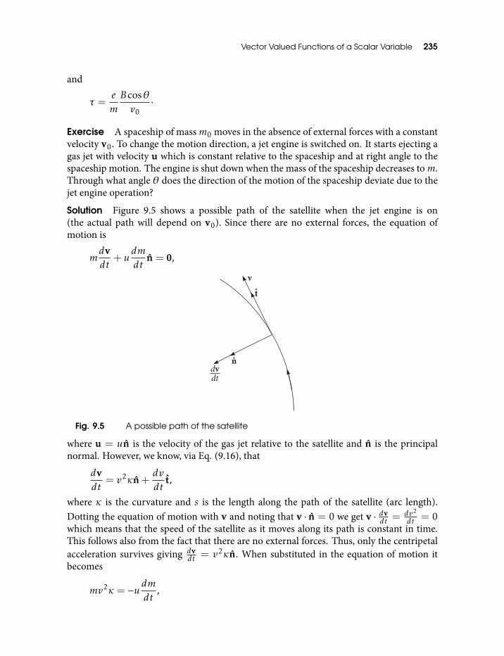
Vector Valued Functions of a Scalar Variable 235
and
τ =emBcosθv0
·
Exercise A spaceship of massm0 moves in the absence of external forces with a constantvelocity v0. To change the motion direction, a jet engine is switched on. It starts ejecting agas jet with velocity u which is constant relative to the spaceship and at right angle to thespaceship motion. The engine is shut down when the mass of the spaceship decreases tom.Through what angle θ does the direction of the motion of the spaceship deviate due to thejet engine operation?
Solution Figure 9.5 shows a possible path of the satellite when the jet engine is on(the actual path will depend on v0). Since there are no external forces, the equation ofmotion is
mdvdt
+ udmdt
n = 0,
Fig. 9.5 A possible path of the satellite
where u = un is the velocity of the gas jet relative to the satellite and n is the principalnormal. However, we know, via Eq. (9.16), that
dvdt
= v2κn+dvdt
t,
where κ is the curvature and s is the length along the path of the satellite (arc length).Dotting the equation of motion with v and noting that v · n = 0 we get v · dv
dt =dv2
dt = 0which means that the speed of the satellite as it moves along its path is constant in time.This follows also from the fact that there are no external forces. Thus, only the centripetalacceleration survives giving dv
dt = v2κn. When substituted in the equation of motion itbecomes
mv2κ = −udmdt
,
236 An Introduction to Vectors, Vector Operators and Vector Analysis
or,
mv2
R= −udm
dt,
or,
dt = −uRv2dmm
.
Here, we have used κ = 1R where R is the radius of curvature. In order to get the angular
advance of the satellite we transform this equation using vdt = Rdθ (which is justifiedbecause the path is continuous and differentiable) to get
Rdθv
= dt = −uRv2dmm
,
or
dθ = −uvdmm
.
Integrating, we get the required angular advance,
θ =
∫dθ = −u
v
∫ m
m0
dmm
=uv
ln(m0
m
).
9.2.1 Normal, rectifying and osculating planes
We fix a point on the curve by fixing t at t0 or s at the corresponding value s0, that is, s0 =s(t0). Let x(t0) = x(s0) = xp be the position vector of this point, say P . The coordinateplanes of the coordinate system given by t, n, b at P are
The plane normal to t, spanned by n, b called normal plane.The plane normal to n, spanned by t, b called rectifying plane andThe plane normal to b, spanned by t, n called osculating plane.These planes are tangent to the space curve at P . Note that these planes change with
the triad t, n, b as the point P moves along the curve or as the parameters t or s change.Therefore, the position vector of a point on each of these planes has to be labelled by eithert or s. So let x(t) be the position vector of an arbitrary point of each of the planes in turn.Then, the equation of the normal plane is, suppressing the parameter,
(x− xp) · t = 0,
the equation of the rectifying plane is
(x− xp) · n = 0,
Vector Valued Functions of a Scalar Variable 237
and the equation of the osculating plane is
(x− xp) · b = 0.
Using the definitions of t and n, we see that b is parallel to x′p × x′′p where prime denotesthe differentiation with respect to s, and this notation will be used subsequently. Thus, theequation to the osculating plane gets the form
(x− xp) · x′p × x′′p = 0.
To get to the t parameterization, note that
x′p = xpdtds
and
x′′p = xp
(dtds
)2
+ xpd2t
ds2.
Exercise Show that xp × xp is parallel to x′p × x′′p .
Hence, the equation for the osculating plane, in terms of t can be written in the form
(x− xp) · xp × xp = 0.
If the curve is a straight line, or a point, xp and xp are parallel, so that equation tothe osculating plane is satisfied by every x in space which means that the equation doesnot determine the osculating plane. For a straight line, the osculating plane is determinedby the choice of the principal normal n (see the text below the place where we havedefined n).
In Cartesian coordinates x,y,z, the equation to the osculating plane becomes∣∣∣∣∣∣∣∣∣∣x − xp y − yp z − zpxp yp zp
xp yp zp
∣∣∣∣∣∣∣∣∣∣= 0.
Exercise Find the equation of the osculating plane to the circular helix.
Answer∣∣∣∣∣∣∣∣∣∣x − acos t y − asin t z − bt
−asin t acos t b
cos t sin t 0
∣∣∣∣∣∣∣∣∣∣= 0,
238 An Introduction to Vectors, Vector Operators and Vector Analysis
or,
xb sin t − ybcos t+ az = abt.
9.2.2 Order of contact
Consider an osculating plane tangent to a space curve x(s) at a point P with position vectorx(s0). In order to estimate how ‘close’ a space curve is to a tangent plane at a point P , wemake use of the concept of order of contact of a plane and a curve. Higher the order ofcontact closer is the plane to the curve. Using this concept we show that the osculatingplane at a point on a space curve is closest to it amongst all the planes tangent to the curveat the same point.
A plane with a common point P at x(s0) with a space curve x(s) has a contact of order nat P if the distance of a point x(s) on the curve from the plane is a function δ(s) satisfying
δ(k)(s0) = 0, k = 0,1, . . . ,n,
δ(n+1)(s0) , 0.
where δ(k) is the kth derivative of δ(s) with respect to s.The distance of a point x(s) on the curve from the osculating plane is
δ(s) = ±[x(s)− x(s0)] · b,
where b = b(s0) is the binormal. We see that
δ(1)(s0) = ±x′(s0) · b = t · b = 0
and
δ(2)(s0) = ±x′′(s0) · b = κn · b = 0,
since the first and the second derivatives of x(s) with respect to s equal t and κnrespectively and t, n, b form an orthonormal triad. Hence, the osculating plane hascontact of at least order two with the curve.
Now consider a second plane tangent to the curve at P . The distance function δ(s) forthis plane is
δ(s) = ±[x(s)− x(s0)] · c
where c is a unit vector normal to the plane. The first two derivatives of δ(s) at P are
δ(1)(s0) = ±x′(s0) · c = t · c
Vector Valued Functions of a Scalar Variable 239
and
δ(2)(s0) = ±x′′(s0) · c = κn · c.
Therefore, the derivatives are non-zero, unless c is parallel to b making two planes coincide.Thus, the order of contact of any plane other than the osculating plane is less than two.
Exercise Find the order of contact of the osculating plane to the circular helix.
Hint We know that the order of contact is at least two. Using the equation of the helix witharc length as parameter, show that δ(3) = ±x′′′(s0) · b = ±ab
c4 , 0, where c =√a2 + b2.
Therefore, the required order of contact is two.
9.2.3 The osculating circle
Let P ,Q,R be three distinct points on a space curve such that the curve has a non-zerocurvature at each of them. Let x(s0),x(s1),x(s2) be the corresponding position vectorswith s0 < s1 < s2. We further assume that the points P ,Q,R also lie on a sphere (x−x0)
2 =a2, x0 being the position vector of the center. We want to find what happens to this spherein the limiting case asQ and R approach P .
We start by defining the function
f (s) = (x(s)− x0)2 − a2,
where s is the arc length parameter. Note that
f (s0) = f (s1) = f (s2) = 0.
Therefore, by Rolle’s theorem, we get,
f ′(ξ1) = f ′(ξ2) = 0, s0 ≤ ξ1 ≤ s1 ≤ ξ2 ≤ s2.
Applying Rolle’s theorem again to f ′(s) we get,
f ′′(ξ3) = 0, ξ1 ≤ ξ3 ≤ ξ2.
AsQ and R approach P , s1,s2,ξ1,ξ2,ξ3 approach s0. Therefore,
f (s0) = (x(s0)− x0)2 − a2 = 0,
f ′(s0) = x′(s0) · (x(s0)− x0) = 0,
f ′′(s0) = x′′(s0) · (x(s0)− x0) + (x′(s0))2 = 0.
Since x′ = t, the second of these equations shows that (x(s0) − x0) lies in the normalplane at P . Therefore, we can express it as a linear combination of n and b, that is,
x(s0)− x0 = αn+ βb. (9.20)
240 An Introduction to Vectors, Vector Operators and Vector Analysis
Since x′′(s0) = κn and x′(s0) = t, the third of the above equations gives,
n · (x(s0)− x0) + ρ = 0, (9.21)
where ρ is the radius of curvature. Dotting Eq. (9.20) with n and then using Eq. (9.21) weget α = −ρ. Squaring each side of Eq. (9.20) and using f (s0) = 0 (first of the above threeequations) we get β = ±
√a2 − ρ2. Using Eq. (9.20) (with the corresponding expressions
for α and β) we see that, for a > ρ, there are two limiting spheres the position vectors ofthe centers of which are given by
x0 = x(s0) + ρn±√a2 − ρ2b. (9.22)
If we select a= ρ then the sphere has its center in the osculating plane. The intersection ofthis sphere and the osculating plane is a circle of radius ρ and is called the osculating circle,or the circle of curvature.
We define the order of contact between two curves in the same way as we did for acurve and a plane. It turns out that the order of contact between the osculating circle andthe space curve is at least two.
9.2.4 Natural equations of a space curve
Two space curves are congruent if they can be made to coincide by only translatingand rotating one of them (that is, via a rigid motion). During a rigid motion, bothcurvature and torsion at all points on the curve remain unaltered. Thus, the samecurvature and torsion, as functions κ(s) and τ(s) of the arc length parameter s, describethe whole class of mutually congruent space curves. The values of κ and τ at a pointcorresponding to s are given by the values of the functions κ(s) and τ(s). This fact isexpressed by the equations
κ = κ(s) and τ = τ(s), (9.23)
which are called the natural, or intrinsic equations of a curve. We know that two congruentcurves have the same natural equations. We now show that the reverse implication is alsotrue: Two curves having the same natural equations are congruent.
Let the two curves be x = x1(s) and x = x2(s). By a rigid motion, we can make thepoints corresponding to s = 0 coincide such that the moving trihedrals at these pointscoincide. Now using Eqs (9.9), (9.13) and (9.14) it is straightforward to show that
dds
(t1 · t2 + n1 · n2 + b1 · b2) = 0,
or,
t1 · t2 + n1 · n2 + b1 · b2 = constant.
Vector Valued Functions of a Scalar Variable 241
However, we know that at s = 0
t1 = t2, n1 = n2, b1 = b2. (9.24)
Therefore,
t1 · t2 + n1 · n2 + b1 · b2 = 3. (9.25)
Since t, n, b are unit vectors, it follows from Eq. (9.25) that
t1 · t2 = n1 · n2 = b1 · b2 = 1
and that Eq. (9.24) applies for all s; not only at s = 0. From t1 · t2 we get,
x′1 = x′2
so that
x1 = x2 + c,
where c is the constant of integration. The initial condition x1(0) = x2(0) gives c = 0.Therefore, for all s
x1 = x2
which means that both the curves are congruent.It can also be shown that given two analytic functions κ(s) > 0 and τ(s) there is a curve
for which the curvature and torsion are given by Eq. (9.23). We skip the proof.We may expand the function x(s) pertaining to the curve in Taylor series (see
section 9.6) around s = 0:
x(s) = x(0) + sx′(0) +s2
2x′′(0) +
s3
3!x′′′(0) + · · · .
Again, expressing the derivatives of x(s) in terms of curvature and torsion via Eqs (9.9),(9.13) and (9.14), we get,
x(s) = x(0) + st(0) +s2
2κ(0)n(0) +
s3
3!
(−κ2(0)t(0) + κ′(0)n(0)
+κ(0)τ(0)b(0))+ · · · .
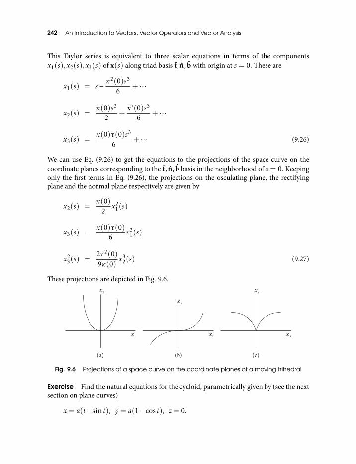
242 An Introduction to Vectors, Vector Operators and Vector Analysis
This Taylor series is equivalent to three scalar equations in terms of the componentsx1(s),x2(s),x3(s) of x(s) along triad basis t, n, b with origin at s = 0. These are
x1(s) = s −κ2(0)s3
6+ · · ·
x2(s) =κ(0)s2
2+κ′(0)s3
6+ · · ·
x3(s) =κ(0)τ(0)s3
6+ · · · (9.26)
We can use Eq. (9.26) to get the equations to the projections of the space curve on thecoordinate planes corresponding to the t, n, b basis in the neighborhood of s = 0. Keepingonly the first terms in Eq. (9.26), the projections on the osculating plane, the rectifyingplane and the normal plane respectively are given by
x2(s) =κ(0)
2x2
1(s)
x3(s) =κ(0)τ(0)
6x3
1(s)
x23(s) =
2τ2(0)9κ(0)
x32(s) (9.27)
These projections are depicted in Fig. 9.6.
Fig. 9.6 Projections of a space curve on the coordinate planes of a moving trihedral
Exercise Find the natural equations for the cycloid, parametrically given by (see the nextsection on plane curves)
x = a(t − sin t), y = a(1− cos t), z = 0.
Vector Valued Functions of a Scalar Variable 243
Solution Since the curve is planar, the unit vector b is a constant vector alwaysperpendicular to the plane of the curve. Therefore, db/ds = 0, that is, τ = 0. To get theequation in κ, we have to find the arc length measured from some fixed point on thecurve, using the given parametric equations. We have,
ds =√dx2 + dy2 = 2asin
t2dt,
giving
s =
∫ s
0ds = 2a
∫ t
πsin
t2dt = −4acos
t2
,
where s is measured from the top of the cycloid, that is, s = 0 at t = π. From Eq. (9.19),the parametric equation of the curve and v = x, a = x we get
κ2 =|[a(1− cos t)i+ asin tj]× [asin ti+ acos tj]|2
[(a(1− cos t)i+ asin tj)2]3=
18a2(1− cos t)
·
Further,
s2 = 16a2 cos2 t2= 8a2(1+ cos t)
giving us the required equation,
1κ2 + s2 = 16a2.
9.2.5 Evolutes and involutes
We shall now use the Frenet–Seret formulae to learn about an important genera of curvescalled evolutes and involutes.
Definition: If there is a one to one correspondence between the points of two curves C1and C2 such that the tangent to C1 at any point on it is normal to C2 at the correspondingpoint on C2 then C1 is called an evolute of C2 and C2 an involute of C1.
We denote all the quantities pertaining to the evolute curve C1 by small case letters,while those pertaining to the involute curve C2 are denoted by the capital letters.
Suppose the equation for the evolute curve C1 is given by x = x(s). We want to find outthe equation for its involute C2 given by X = X(S). We refer to Fig. 9.7. If the distance P1P2is taken to be u, the position vector OP2 will be X = x + ut where x = x(s) and t = dx
ds .Differentiating with respect to S, the arc length parameter of the involute, we get
dXdS
= T = (x′ + ut′ + u′ t)dsdS
.
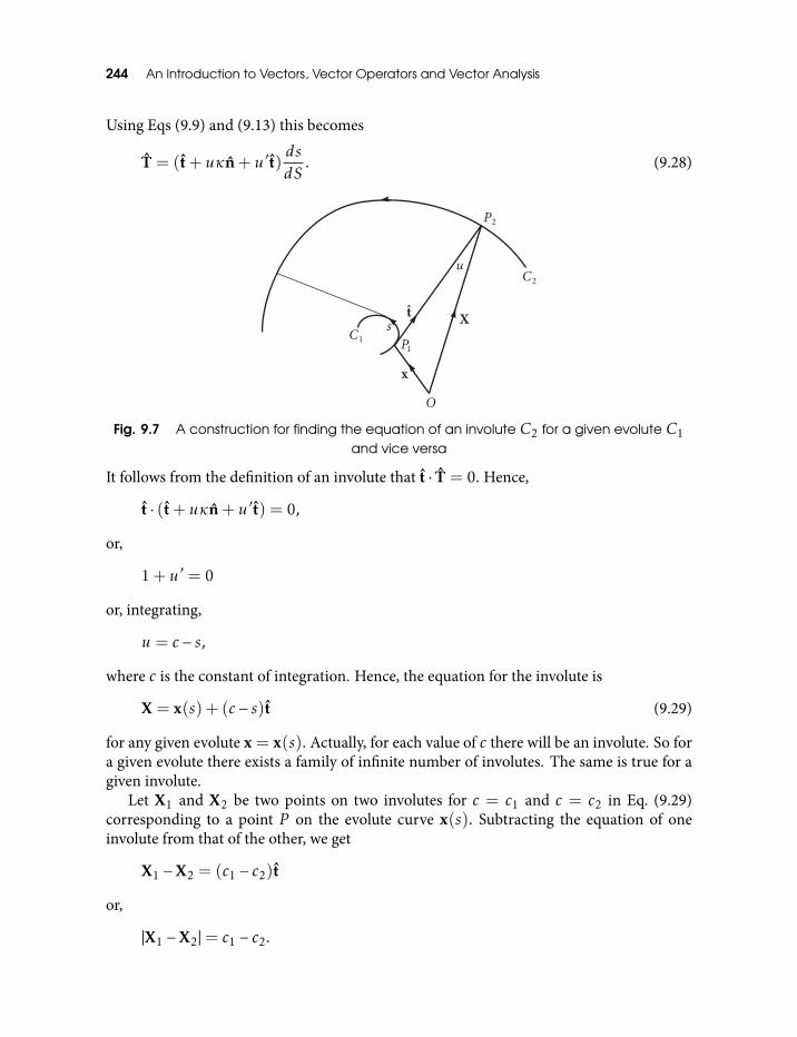
244 An Introduction to Vectors, Vector Operators and Vector Analysis
Using Eqs (9.9) and (9.13) this becomes
T = (t+ uκn+ u′ t)dsdS
. (9.28)
Fig. 9.7 A construction for finding the equation of an involute C2 for a given evolute C1and vice versa
It follows from the definition of an involute that t · T = 0. Hence,
t · (t+ uκn+ u′ t) = 0,
or,
1+ u′ = 0
or, integrating,
u = c − s,
where c is the constant of integration. Hence, the equation for the involute is
X = x(s) + (c − s)t (9.29)
for any given evolute x = x(s). Actually, for each value of c there will be an involute. So fora given evolute there exists a family of infinite number of involutes. The same is true for agiven involute.
Let X1 and X2 be two points on two involutes for c = c1 and c = c2 in Eq. (9.29)corresponding to a point P on the evolute curve x(s). Subtracting the equation of oneinvolute from that of the other, we get
X1 −X2 = (c1 − c2)t
or,
|X1 −X2|= c1 − c2.
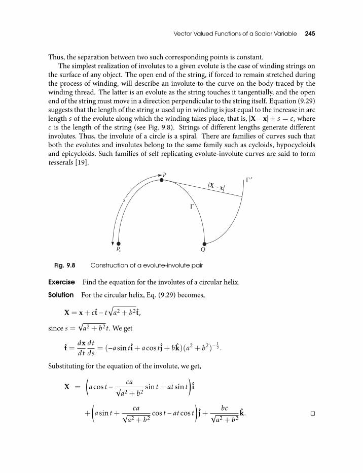
Vector Valued Functions of a Scalar Variable 245
Thus, the separation between two such corresponding points is constant.The simplest realization of involutes to a given evolute is the case of winding strings on
the surface of any object. The open end of the string, if forced to remain stretched duringthe process of winding, will describe an involute to the curve on the body traced by thewinding thread. The latter is an evolute as the string touches it tangentially, and the openend of the string must move in a direction perpendicular to the string itself. Equation (9.29)suggests that the length of the string u used up in winding is just equal to the increase in arclength s of the evolute along which the winding takes place, that is, |X− x|+ s = c, wherec is the length of the string (see Fig. 9.8). Strings of different lengths generate differentinvolutes. Thus, the involute of a circle is a spiral. There are families of curves such thatboth the evolutes and involutes belong to the same family such as cycloids, hypocycloidsand epicycloids. Such families of self replicating evolute-involute curves are said to formtesserals [19].
Fig. 9.8 Construction of a evolute-involute pair
Exercise Find the equation for the involutes of a circular helix.
Solution For the circular helix, Eq. (9.29) becomes,
X = x+ ct− t√a2 + b2t,
since s =√a2 + b2t. We get
t =dxdtdtds
= (−asin ti+ acos tj+ bk)(a2 + b2)−12 .
Substituting for the equation of the involute, we get,
X =
(acos t − ca
√a2 + b2
sin t+ at sin t)
i
+
(asin t+
ca√a2 + b2
cos t − at cos t)
j+bc
√a2 + b2
k.
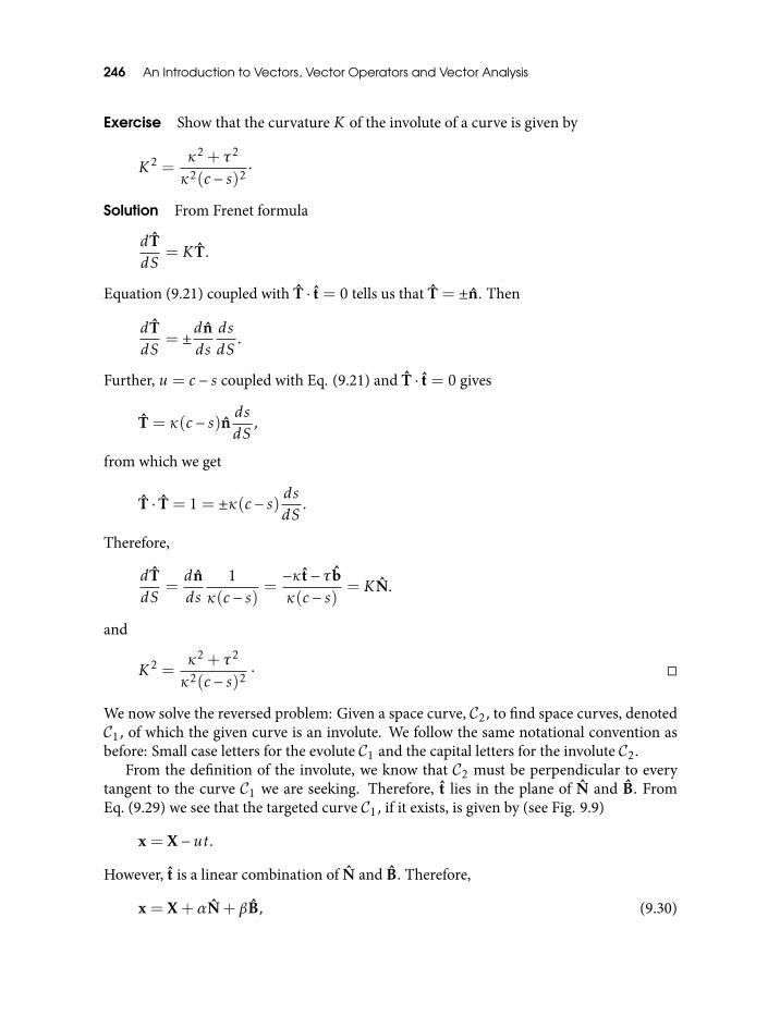
246 An Introduction to Vectors, Vector Operators and Vector Analysis
Exercise Show that the curvature K of the involute of a curve is given by
K2 =κ2 + τ2
κ2(c − s)2 ·
Solution From Frenet formula
dTdS
= KT.
Equation (9.21) coupled with T · t = 0 tells us that T = ±n. Then
dTdS
= ±dnds
dsdS
.
Further, u = c − s coupled with Eq. (9.21) and T · t = 0 gives
T = κ(c − s)n dsdS
,
from which we get
T · T = 1 = ±κ(c − s) dsdS
.
Therefore,
dTdS
=dnds
1κ(c − s)
=−κt− τbκ(c − s)
= KN.
and
K2 =κ2 + τ2
κ2(c − s)2 ·
We now solve the reversed problem: Given a space curve, C2, to find space curves, denotedC1, of which the given curve is an involute. We follow the same notational convention asbefore: Small case letters for the evolute C1 and the capital letters for the involute C2.
From the definition of the involute, we know that C2 must be perpendicular to everytangent to the curve C1 we are seeking. Therefore, t lies in the plane of N and B. FromEq. (9.29) we see that the targeted curve C1, if it exists, is given by (see Fig. 9.9)
x = X−ut.
However, t is a linear combination of N and B. Therefore,
x = X+αN+ βB, (9.30)
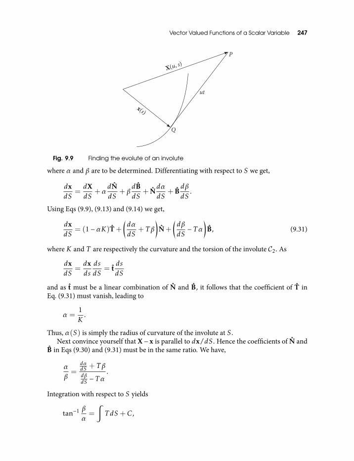
Vector Valued Functions of a Scalar Variable 247
Fig. 9.9 Finding the evolute of an involute
where α and β are to be determined. Differentiating with respect to S we get,
dxdS
=dXdS
+αdNdS
+ βdBdS
+ NdαdS
+ Bdβ
dS.
Using Eqs (9.9), (9.13) and (9.14) we get,
dxdS
= (1−αK)T+
(dαdS
+ T β
)N+
(dβ
dS− T α
)B, (9.31)
where K and T are respectively the curvature and the torsion of the involute C2. As
dxdS
=dxds
dsdS
= tdsdS
and as t must be a linear combination of N and B, it follows that the coefficient of T inEq. (9.31) must vanish, leading to
α =1K
.
Thus, α(S) is simply the radius of curvature of the involute at S.Next convince yourself that X− x is parallel to dx/dS. Hence the coefficients of N and
B in Eqs (9.30) and (9.31) must be in the same ratio. We have,
αβ=
dαdS + T βdβdS − T α
.
Integration with respect to S yields
tan−1 β
α=
∫T dS +C,

248 An Introduction to Vectors, Vector Operators and Vector Analysis
or,
β = α
[tan
(∫T dS +C
)],
where C is a constant of integration. Substituting the values of α and β in Eq. (9.30) we getthe equation of the evolute:
x = X+1K
N+1K
[tan
(∫T dS +C
)]B. (9.32)
Note that for a point P of the involute the corresponding pointsQ1(x1),Q2(x2), . . . on theevolutes for different values of C C1,C2, . . . lie on a straight line parallel to the binormalB at P because xi − xj , i , j, i, j = 1,2, . . . is proportional to B. Further, this line is ata distance of 1
K (radius of curvature at P ) because x has a component along N which isnormal to B and has magnitude 1
K .
Exercise Obtain the equations for the evolutes of the circular helix.
Hint Specialize Eq. (9.32) to circular helix. All the required results are available in previousexercises.
9.3 Plane CurvesA separate study of plane curves, that is, curves on a plane, is worthwhile, because manyaspects of the theory can be developed with them without losing generality and manycharacteristics of geometric parameters for these curves can be defined, which have noanalogue for curves in three dimensional space. Thus, for example, we can define the signof curvature, κ, for a plane curve, positive and negative sides of a plane curve or theinterior and the exterior regions of a closed plane curve, all of which are not meaningfulfor a curve in three dimensional space.
A plane curve is parameterized by a vector valued function x(t) of parameter t wherex(t) ≡ (x(t),y(t)) is a planar vector with coordinate functions (x(t),y(t)). We assumethat the functions x(t) ≡ (x(t),y(t)) possess continuous derivatives with respect to t.
9.3.1 Three different parameterizations of an ellipse
We give three different ways to parameterize ellipse, first by the so called eccentric angle(called eccentric anomaly by the astronomers), the second by using the angle swept by thevector based at one of the foci counterclockwise from its pericenter (called true anomaly bythe astronomers) and the third using the time taken by a planet to reach a given point on itselliptical path around the sun assuming t = 0 at the pericenter. On the way we shall pick upsome geometrical characteristics of ellipse and also some of its physical realizations, mostprominant being planetary motion.
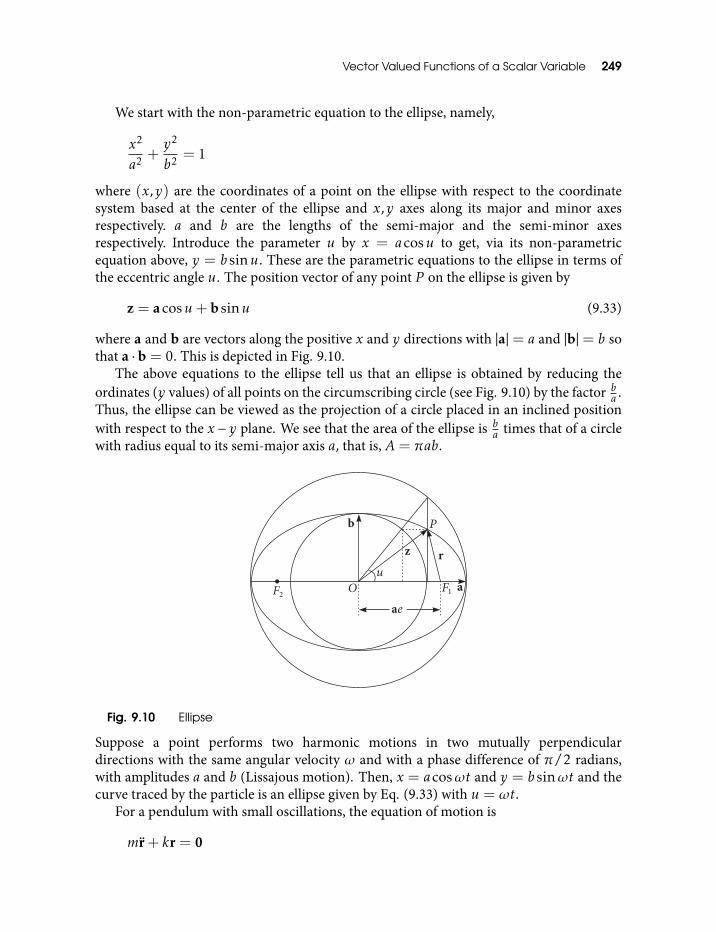
Vector Valued Functions of a Scalar Variable 249
We start with the non-parametric equation to the ellipse, namely,
x2
a2 +y2
b2 = 1
where (x,y) are the coordinates of a point on the ellipse with respect to the coordinatesystem based at the center of the ellipse and x,y axes along its major and minor axesrespectively. a and b are the lengths of the semi-major and the semi-minor axesrespectively. Introduce the parameter u by x = acosu to get, via its non-parametricequation above, y = b sinu. These are the parametric equations to the ellipse in terms ofthe eccentric angle u. The position vector of any point P on the ellipse is given by
z = acosu+bsinu (9.33)
where a and b are vectors along the positive x and y directions with |a|= a and |b|= b sothat a ·b = 0. This is depicted in Fig. 9.10.
The above equations to the ellipse tell us that an ellipse is obtained by reducing theordinates (y values) of all points on the circumscribing circle (see Fig. 9.10) by the factor ba .Thus, the ellipse can be viewed as the projection of a circle placed in an inclined positionwith respect to the x − y plane. We see that the area of the ellipse is b
a times that of a circlewith radius equal to its semi-major axis a, that is, A= πab.
Fig. 9.10 Ellipse
Suppose a point performs two harmonic motions in two mutually perpendiculardirections with the same angular velocity ω and with a phase difference of π/2 radians,with amplitudes a and b (Lissajous motion). Then, x = acosωt and y = b sinωt and thecurve traced by the particle is an ellipse given by Eq. (9.33) with u = ωt.
For a pendulum with small oscillations, the equation of motion is
mr+ kr = 0
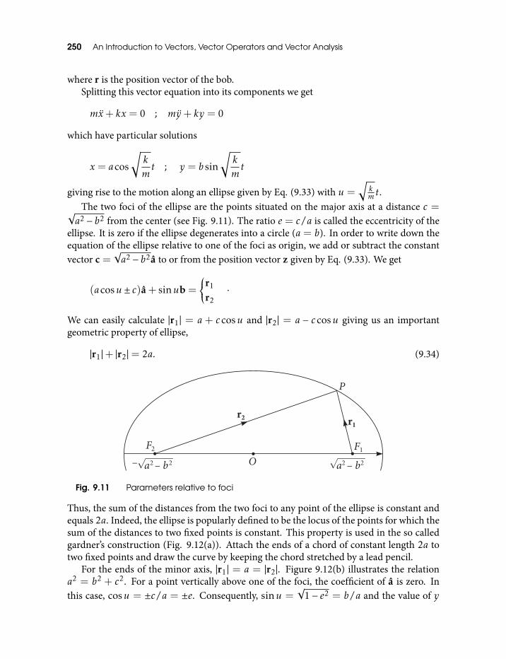
250 An Introduction to Vectors, Vector Operators and Vector Analysis
where r is the position vector of the bob.Splitting this vector equation into its components we get
mx+ kx = 0 ; my+ ky = 0
which have particular solutions
x = acos
√kmt ; y = b sin
√kmt
giving rise to the motion along an ellipse given by Eq. (9.33) with u =√
km t.
The two foci of the ellipse are the points situated on the major axis at a distance c =√a2 − b2 from the center (see Fig. 9.11). The ratio e = c/a is called the eccentricity of the
ellipse. It is zero if the ellipse degenerates into a circle (a = b). In order to write down theequation of the ellipse relative to one of the foci as origin, we add or subtract the constantvector c =
√a2 − b2a to or from the position vector z given by Eq. (9.33). We get
(acosu ± c)a+ sinub =
r1
r2·
We can easily calculate |r1| = a+ ccosu and |r2| = a − ccosu giving us an importantgeometric property of ellipse,
|r1|+ |r2|= 2a. (9.34)
Fig. 9.11 Parameters relative to foci
Thus, the sum of the distances from the two foci to any point of the ellipse is constant andequals 2a. Indeed, the ellipse is popularly defined to be the locus of the points for which thesum of the distances to two fixed points is constant. This property is used in the so calledgardner’s construction (Fig. 9.12(a)). Attach the ends of a chord of constant length 2a totwo fixed points and draw the curve by keeping the chord stretched by a lead pencil.
For the ends of the minor axis, |r1| = a = |r2|. Figure 9.12(b) illustrates the relationa2 = b2 + c2. For a point vertically above one of the foci, the coefficient of a is zero. Inthis case, cosu = ±c/a = ±e. Consequently, sinu =
√1− e2 = b/a and the value of y
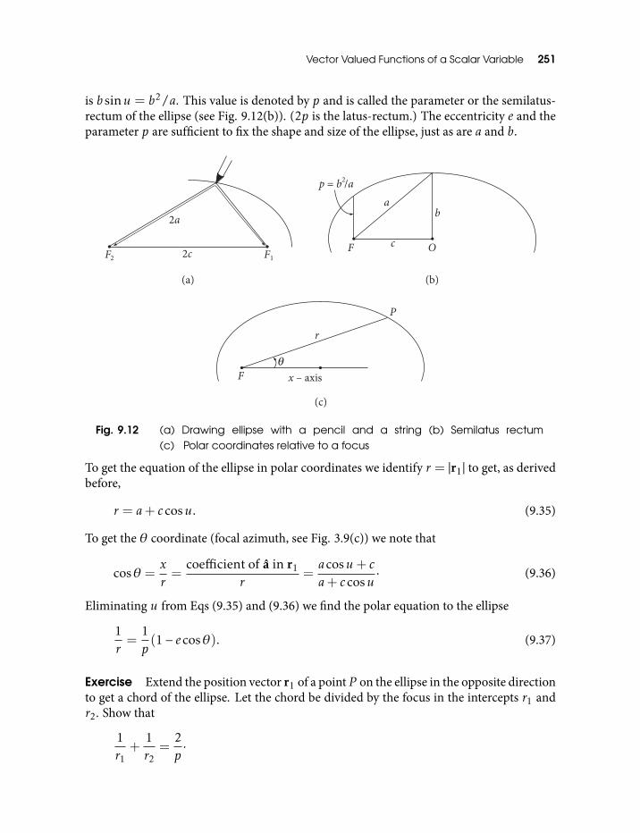
Vector Valued Functions of a Scalar Variable 251
is b sinu = b2/a. This value is denoted by p and is called the parameter or the semilatus-rectum of the ellipse (see Fig. 9.12(b)). (2p is the latus-rectum.) The eccentricity e and theparameter p are sufficient to fix the shape and size of the ellipse, just as are a and b.
Fig. 9.12 (a) Drawing ellipse with a pencil and a string (b) Semilatus rectum(c) Polar coordinates relative to a focus
To get the equation of the ellipse in polar coordinates we identify r = |r1| to get, as derivedbefore,
r = a+ ccosu. (9.35)
To get the θ coordinate (focal azimuth, see Fig. 3.9(c)) we note that
cosθ =xr=
coefficient of a in r1
r=acosu+ ca+ ccosu
· (9.36)
Eliminating u from Eqs (9.35) and (9.36) we find the polar equation to the ellipse
1r=
1p(1− ecosθ). (9.37)
Exercise Extend the position vector r1 of a point P on the ellipse in the opposite directionto get a chord of the ellipse. Let the chord be divided by the focus in the intercepts r1 andr2. Show that
1r1
+1r2
=2p·
252 An Introduction to Vectors, Vector Operators and Vector Analysis
Hint Use Eq. (9.37) for r1 and r2 and note that cos(θ+π) = −cosθ. Thus, each chordpassing through the focus is divided by it into two parts such that their hamonic mean isconstant and equals p.
Thus, we have parameterized ellipse using the eccentric angle u with origin at the centerof the ellipse and using the polar coordinate θ with origin at one of the foci. We canparameterize ellipse by the time of travel of a particle moving on it, tracing it in the senseof increasing t, taking t = 0 when the particle was at the pericenter. Typical realization ofthis situation is the motion of planets along their elliptic orbits around the sun, which sitsat one of the foci and interacts gravitationally with the planet. Actually, we are going tore-parameterize the elliptical path of the planet by expressing t in terms of the eccentricanomaly u.
We start with re-writing Eq. (9.33) as
r = z− ea = a(cosu − e) +bsinu, (9.38)
which is a parametric equation r = r(u) of the elliptic orbit. Now the task is to determinethe parameter u as a function of time u = u(t) so that Eq. (9.38) directly gives thedependence of r on t, r = r(t). From Eq. (9.38) we get, for the specific angularmomentum (angular momentum per unit mass),
H = r× r = z× z− ea× z,
or,
Hdt = z× dz− ea× dz.
From Eq. (9.33) we get
dz = −asinudu+bcosudu, (9.39)
so that using Eqs (9.33) and (9.39) we have
z× dz = a×bdu.
Similarly,
a× dz = a×bcosudu.
Therefore, Hdt becomes
Hdt = a×bdu − ea×bcosudu. (9.40)
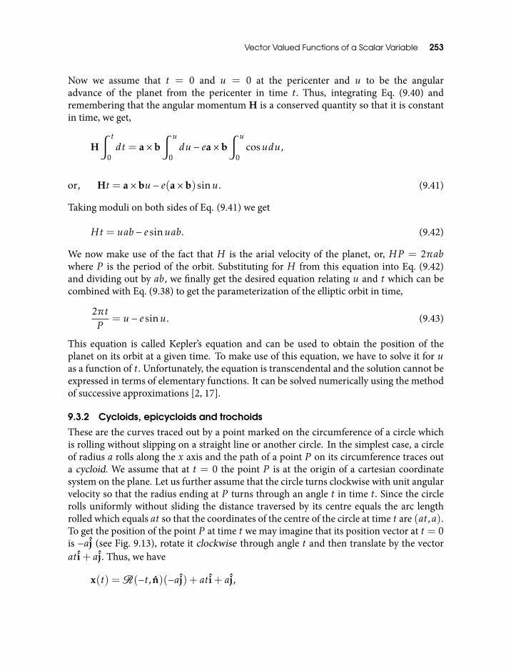
Vector Valued Functions of a Scalar Variable 253
Now we assume that t = 0 and u = 0 at the pericenter and u to be the angularadvance of the planet from the pericenter in time t. Thus, integrating Eq. (9.40) andremembering that the angular momentum H is a conserved quantity so that it is constantin time, we get,
H∫ t
0dt = a×b
∫ u
0du − ea×b
∫ u
0cosudu,
or, Ht = a×bu − e(a×b)sinu. (9.41)
Taking moduli on both sides of Eq. (9.41) we get
Ht = uab − e sinuab. (9.42)
We now make use of the fact that H is the arial velocity of the planet, or, HP = 2πabwhere P is the period of the orbit. Substituting for H from this equation into Eq. (9.42)and dividing out by ab, we finally get the desired equation relating u and t which can becombined with Eq. (9.38) to get the parameterization of the elliptic orbit in time,
2πtP
= u − e sinu. (9.43)
This equation is called Kepler’s equation and can be used to obtain the position of theplanet on its orbit at a given time. To make use of this equation, we have to solve it for uas a function of t. Unfortunately, the equation is transcendental and the solution cannot beexpressed in terms of elementary functions. It can be solved numerically using the methodof successive approximations [2, 17].
9.3.2 Cycloids, epicycloids and trochoids
These are the curves traced out by a point marked on the circumference of a circle whichis rolling without slipping on a straight line or another circle. In the simplest case, a circleof radius a rolls along the x axis and the path of a point P on its circumference traces outa cycloid. We assume that at t = 0 the point P is at the origin of a cartesian coordinatesystem on the plane. Let us further assume that the circle turns clockwise with unit angularvelocity so that the radius ending at P turns through an angle t in time t. Since the circlerolls uniformly without sliding the distance traversed by its centre equals the arc lengthrolled which equals at so that the coordinates of the centre of the circle at time t are (at,a).To get the position of the point P at time t we may imagine that its position vector at t = 0is −aj (see Fig. 9.13), rotate it clockwise through angle t and then translate by the vectorati+ aj. Thus, we have
x(t) =R(−t, n)(−aj) + ati+ aj,
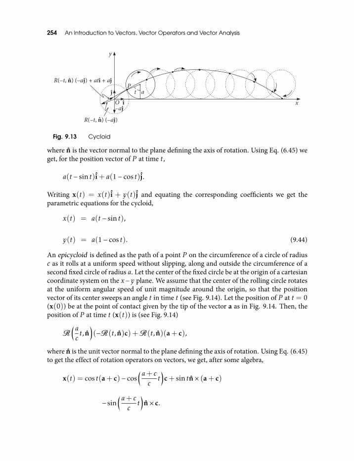
254 An Introduction to Vectors, Vector Operators and Vector Analysis
Fig. 9.13 Cycloid
where n is the vector normal to the plane defining the axis of rotation. Using Eq. (6.45) weget, for the position vector of P at time t,
a(t − sin t)i+ a(1− cos t)j.
Writing x(t) = x(t)i + y(t)j and equating the corresponding coefficients we get theparametric equations for the cycloid,
x(t) = a(t − sin t),
y(t) = a(1− cos t). (9.44)
An epicycloid is defined as the path of a point P on the circumference of a circle of radiusc as it rolls at a uniform speed without slipping, along and outside the circumference of asecond fixed circle of radius a. Let the center of the fixed circle be at the origin of a cartesiancoordinate system on the x−y plane. We assume that the center of the rolling circle rotatesat the uniform angular speed of unit magnitude around the origin, so that the positionvector of its center sweeps an angle t in time t (see Fig. 9.14). Let the position of P at t = 0(x(0)) be at the point of contact given by the tip of the vector a as in Fig. 9.14. Then, theposition of P at time t (x(t)) is (see Fig. 9.14)
R(act, n
)(−R(t, n)c) +R(t, n)(a+ c),
where n is the unit vector normal to the plane defining the axis of rotation. Using Eq. (6.45)to get the effect of rotation operators on vectors, we get, after some algebra,
x(t) = cos t(a+ c)− cos(a+ cct)
c+ sin tn× (a+ c)
−sin(a+ cct)
n× c.
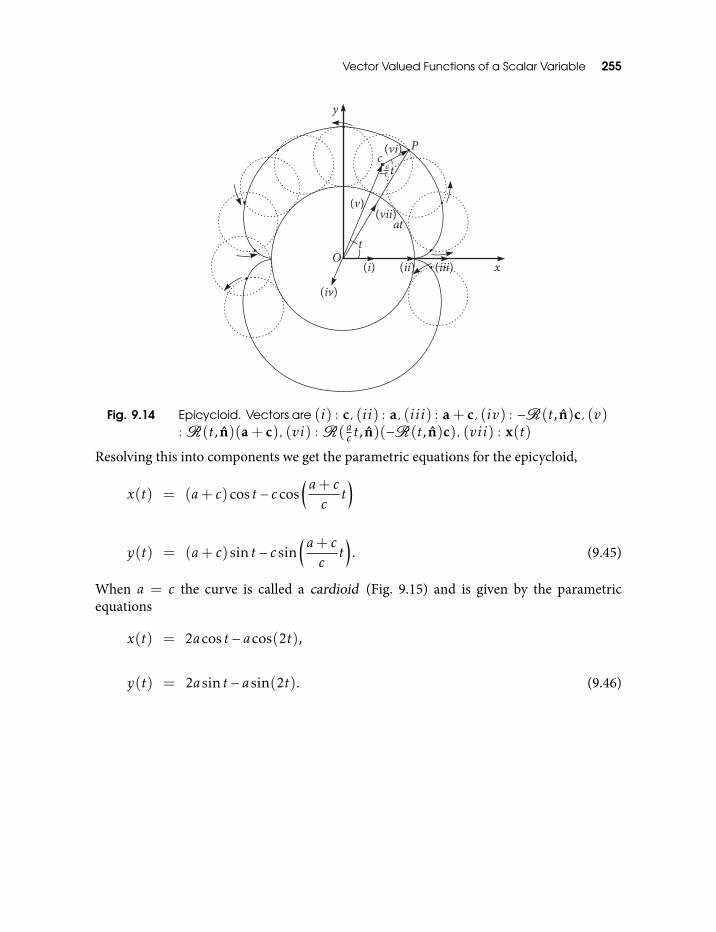
Vector Valued Functions of a Scalar Variable 255
Fig. 9.14 Epicycloid. Vectors are (i) : c, (ii) : a, (iii) : a+ c, (iv) : −R(t, n)c, (v): R(t, n)(a+ c), (vi) : R( ac t, n)(−R(t, n)c), (vii) : x(t)
Resolving this into components we get the parametric equations for the epicycloid,
x(t) = (a+ c)cos t − ccos(a+ cct)
y(t) = (a+ c)sin t − c sin(a+ cct)
. (9.45)
When a = c the curve is called a cardioid (Fig. 9.15) and is given by the parametricequations
x(t) = 2acos t − acos(2t),
y(t) = 2asin t − asin(2t). (9.46)
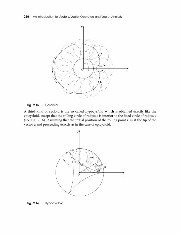
256 An Introduction to Vectors, Vector Operators and Vector Analysis
Fig. 9.15 Cardioid
A third kind of cycloid is the so called hypocycloid which is obtained exactly like theepicycloid, except that the rolling circle of radius c is interior to the fixed circle of radius a(see Fig. 9.16). Assuming that the initial position of the rolling point P is at the tip of thevector a and proceeding exactly as in the case of epicycloid,
Fig. 9.16 Hypocycloid
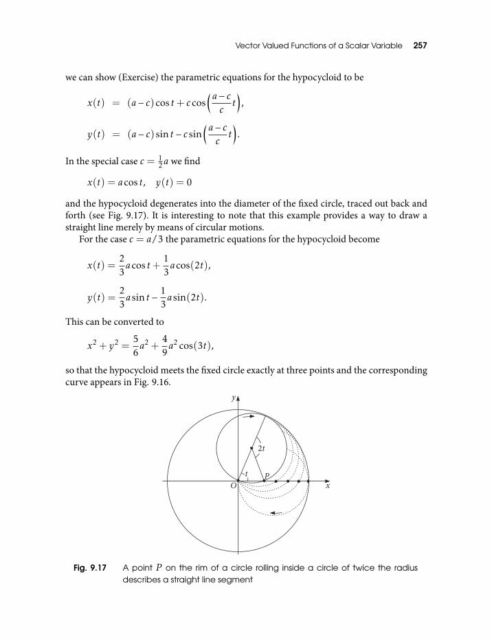
Vector Valued Functions of a Scalar Variable 257
we can show (Exercise) the parametric equations for the hypocycloid to be
x(t) = (a− c)cos t+ ccos(a− cct)
,
y(t) = (a− c)sin t − c sin(a− cct)
.
In the special case c = 12a we find
x(t) = acos t, y(t) = 0
and the hypocycloid degenerates into the diameter of the fixed circle, traced out back andforth (see Fig. 9.17). It is interesting to note that this example provides a way to draw astraight line merely by means of circular motions.
For the case c = a/3 the parametric equations for the hypocycloid become
x(t) =23acos t+
13acos(2t),
y(t) =23asin t − 1
3asin(2t).
This can be converted to
x2 + y2 =56a2 +
49a2 cos(3t),
so that the hypocycloid meets the fixed circle exactly at three points and the correspondingcurve appears in Fig. 9.16.
Fig. 9.17 A point P on the rim of a circle rolling inside a circle of twice the radiusdescribes a straight line segment
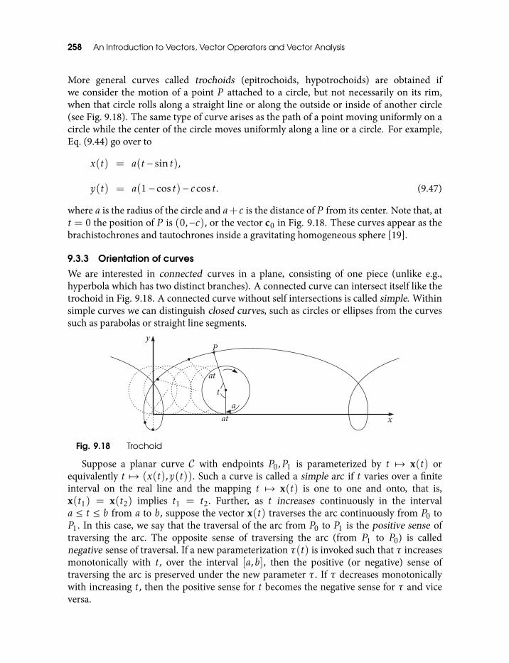
258 An Introduction to Vectors, Vector Operators and Vector Analysis
More general curves called trochoids (epitrochoids, hypotrochoids) are obtained ifwe consider the motion of a point P attached to a circle, but not necessarily on its rim,when that circle rolls along a straight line or along the outside or inside of another circle(see Fig. 9.18). The same type of curve arises as the path of a point moving uniformly on acircle while the center of the circle moves uniformly along a line or a circle. For example,Eq. (9.44) go over to
x(t) = a(t − sin t),
y(t) = a(1− cos t)− ccos t. (9.47)
where a is the radius of the circle and a+ c is the distance of P from its center. Note that, att = 0 the position of P is (0,−c), or the vector c0 in Fig. 9.18. These curves appear as thebrachistochrones and tautochrones inside a gravitating homogeneous sphere [19].
9.3.3 Orientation of curves
We are interested in connected curves in a plane, consisting of one piece (unlike e.g.,hyperbola which has two distinct branches). A connected curve can intersect itself like thetrochoid in Fig. 9.18. A connected curve without self intersections is called simple. Withinsimple curves we can distinguish closed curves, such as circles or ellipses from the curvessuch as parabolas or straight line segments.
Fig. 9.18 Trochoid
Suppose a planar curve C with endpoints P0,P1 is parameterized by t 7→ x(t) orequivalently t 7→ (x(t),y(t)). Such a curve is called a simple arc if t varies over a finiteinterval on the real line and the mapping t 7→ x(t) is one to one and onto, that is,x(t1) = x(t2) implies t1 = t2. Further, as t increases continuously in the intervala ≤ t ≤ b from a to b, suppose the vector x(t) traverses the arc continuously from P0 toP1. In this case, we say that the traversal of the arc from P0 to P1 is the positive sense oftraversing the arc. The opposite sense of traversing the arc (from P1 to P0) is callednegative sense of traversal. If a new parameterization τ(t) is invoked such that τ increasesmonotonically with t, over the interval [a,b], then the positive (or negative) sense oftraversing the arc is preserved under the new parameter τ . If τ decreases monotonicallywith increasing t, then the positive sense for t becomes the negative sense for τ and viceversa.
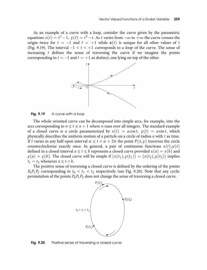
Vector Valued Functions of a Scalar Variable 259
As an example of a curve with a loop, consider the curve given by the parametricequations x(t) = t2 − 1, y(t) = t3 − t. As t varies from −∞ to +∞ the curve crosses theorigin twice for t = −1 and t = +1 while x(t) is unique for all other values of t(Fig. 9.19). The interval −1 < t < +1 corresponds to a loop of the curve. The sense ofincreasing t defines the sense of traversing the curve if we imagine the pointscorresponding to t = −1 and t = +1 as distinct, one lying on top of the other.
Fig. 9.19 A curve with a loop
The whole oriented curve can be decomposed into simple arcs, for example, into thearcs corresponding to n ≤ t ≤ n+ 1 where n runs over all integers. The standard exampleof a closed curve is a circle parameterized by x(t) = acos t, y(t) = asin t, whichphysically describes the uniform motion of a particle on a circle of radius a with t as time.If t varies in any half-open interval α ≤ t < α + 2π the point P (x,y) traverses the circlecounterclockwise exactly once. In general, a pair of continuous functions x(t),y(t)defined in a closed interval a ≤ t ≤ b represents a closed curve provided x(a) = x(b) andy(a) = y(b). The closed curve will be simple if (x(t1),y(t1)) = (x(t2),y(t2)) impliest1 = t2 whenever a ≤ t < b.
The positive sense of traversing a closed curve is defined by the ordering of the pointsP0P1P2 corresponding to t0 < t1 < t2 respectively (see Fig. 9.20). Note that any cyclicpermutation of the points P0P1P2 does not change the sense of traversing a closed curve.
Fig. 9.20 Positive sense of traversing a closed curve
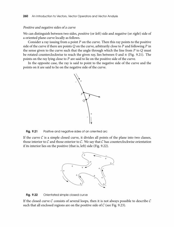
260 An Introduction to Vectors, Vector Operators and Vector Analysis
Positive and negative sides of a curve
We can distinguish between two sides, positive (or left) side and negative (or right) side ofa oriented plane curve locally as follows.
Consider a ray issuing from a point P on the curve. Then this ray points to the positiveside of the curve if there are pointsQ on the curve, arbitrarily close to P and following P inthe sense given to the curve such that the angle through which the line from P to Q mustbe rotated counterclockwise to reach the given ray, lies between 0 and π (Fig. 9.21). Thepoints on the ray lying close to P are said to lie on the positive side of the curve.
In the opposite case, the ray is said to point to the negative side of the curve and thepoints on it are said to lie on the negative side of the curve.
Fig. 9.21 Positive and negative sides of an oriented arc
If the curve C is a simple closed curve, it divides all points of the plane into two classes,those interior to C and those exterior to C. We say that C has counterclockwise orientationif its interior lies on the positive (that is, left) side (Fig. 9.22).
Fig. 9.22 Orientated simple closed curve
If the closed curve C consists of several loops, then it is not always possible to describe Csuch that all enclosed regions are on the positive side of C (see Fig. 9.23).
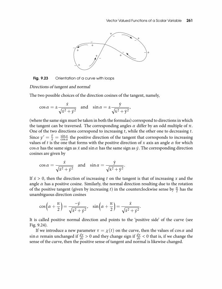
Vector Valued Functions of a Scalar Variable 261
Fig. 9.23 Orientation of a curve with loops
Directions of tangent and normal
The two possible choices of the direction cosines of the tangent, namely,
cosα = ± x√x2 + y2
and sinα = ± y√x2 + y2
,
(where the same sign must be taken in both the formulas) correspond to directions in whichthe tangent can be traversed. The corresponding angles α differ by an odd multiple of π.One of the two directions correspond to increasing t, while the other one to decreasing t.Since y′ = y
x = sinαcosα the positive direction of the tangent that corresponds to increasing
values of t is the one that forms with the positive direction of x axis an angle α for whichcosα has the same sign as x and sinα has the same sign as y. The corresponding directioncosines are given by
cosα =x√
x2 + y2and sinα =
y√x2 + y2
.
If x > 0, then the direction of increasing t on the tangent is that of increasing x and theangle α has a positive cosine. Similarly, the normal direction resulting due to the rotationof the positive tangent (given by increasing t) in the counterclockwise sense by π
2 has theunambiguous direction cosines
cos(α+
π2
)=
−y√x2 + y2
, sin(α+
π2
)=
x√x2 + y2
.
It is called positive normal direction and points to the ‘positive side’ of the curve (seeFig. 9.24).
If we introduce a new parameter τ = χ(t) on the curve, then the values of cosα andsinα remain unchanged if dτdt > 0 and they change sign if dτdt < 0 that is, if we change thesense of the curve, then the positive sense of tangent and normal is likewise changed.
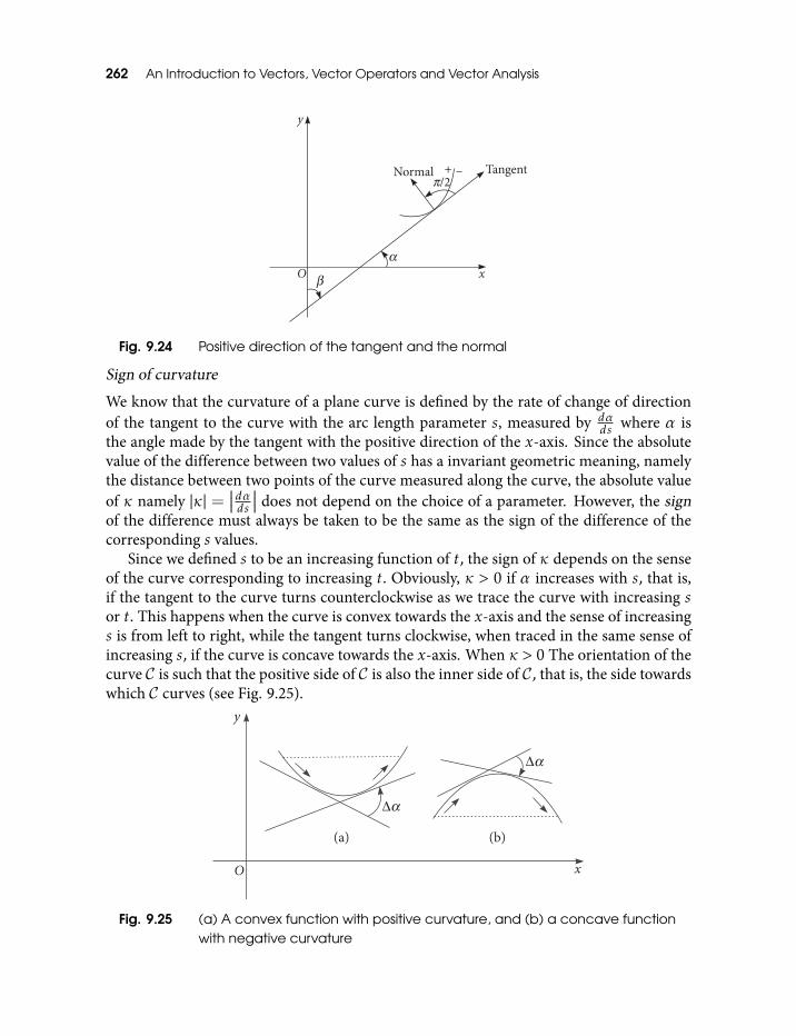
262 An Introduction to Vectors, Vector Operators and Vector Analysis
Fig. 9.24 Positive direction of the tangent and the normal
Sign of curvature
We know that the curvature of a plane curve is defined by the rate of change of directionof the tangent to the curve with the arc length parameter s, measured by dα
ds where α isthe angle made by the tangent with the positive direction of the x-axis. Since the absolutevalue of the difference between two values of s has a invariant geometric meaning, namelythe distance between two points of the curve measured along the curve, the absolute valueof κ namely |κ| =
∣∣∣dαds
∣∣∣ does not depend on the choice of a parameter. However, the signof the difference must always be taken to be the same as the sign of the difference of thecorresponding s values.
Since we defined s to be an increasing function of t, the sign of κ depends on the senseof the curve corresponding to increasing t. Obviously, κ > 0 if α increases with s, that is,if the tangent to the curve turns counterclockwise as we trace the curve with increasing sor t. This happens when the curve is convex towards the x-axis and the sense of increasings is from left to right, while the tangent turns clockwise, when traced in the same sense ofincreasing s, if the curve is concave towards the x-axis. When κ > 0 The orientation of thecurve C is such that the positive side of C is also the inner side of C, that is, the side towardswhich C curves (see Fig. 9.25).
Fig. 9.25 (a) A convex function with positive curvature, and (b) a concave functionwith negative curvature
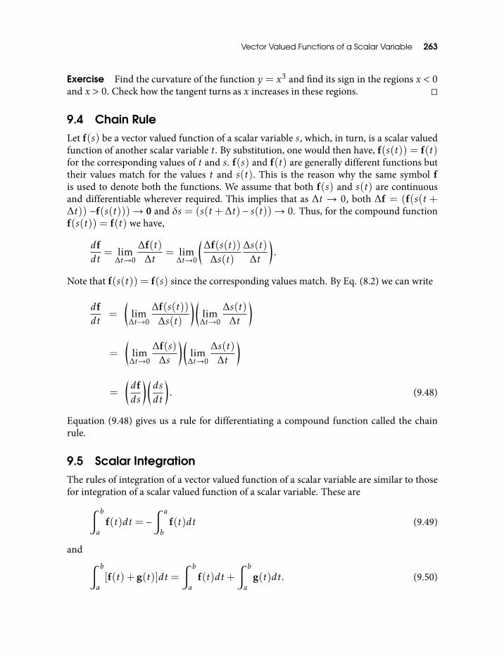
Vector Valued Functions of a Scalar Variable 263
Exercise Find the curvature of the function y = x3 and find its sign in the regions x < 0and x > 0. Check how the tangent turns as x increases in these regions.
9.4 Chain RuleLet f(s) be a vector valued function of a scalar variable s, which, in turn, is a scalar valuedfunction of another scalar variable t. By substitution, one would then have, f(s(t)) = f(t)for the corresponding values of t and s. f(s) and f(t) are generally different functions buttheir values match for the values t and s(t). This is the reason why the same symbol fis used to denote both the functions. We assume that both f(s) and s(t) are continuousand differentiable wherever required. This implies that as ∆t → 0, both ∆f = (f(s(t +∆t)) −f(s(t)))→ 0 and δs = (s(t+∆t) − s(t))→ 0. Thus, for the compound functionf(s(t)) = f(t) we have,
dfdt
= lim∆t→0
∆f(t)∆t
= lim∆t→0
(∆f(s(t))∆s(t)
∆s(t)
∆t
).
Note that f(s(t)) = f(s) since the corresponding values match. By Eq. (8.2) we can write
dfdt
=
(lim∆t→0
∆f(s(t))∆s(t)
)(lim∆t→0
∆s(t)
∆t
)
=
(lim∆t→0
∆f(s)∆s
)(lim∆t→0
∆s(t)
∆t
)
=
(dfds
)(dsdt
). (9.48)
Equation (9.48) gives us a rule for differentiating a compound function called the chainrule.
9.5 Scalar IntegrationThe rules of integration of a vector valued function of a scalar variable are similar to thosefor integration of a scalar valued function of a scalar variable. These are∫ b
af(t)dt = −
∫ a
bf(t)dt (9.49)
and ∫ b
a[f(t) + g(t)]dt =
∫ b
af(t)dt+
∫ b
ag(t)dt. (9.50)
264 An Introduction to Vectors, Vector Operators and Vector Analysis
For a < c < b,∫ b
af(t)dt =
∫ c
af(t)dt+
∫ b
cf(t)dt. (9.51)
If a is a constant vector independent of t, then,∫ b
aa · f(t)dt = a ·
[∫ b
af(t)dt
],
∫ b
aa× f(t)dt = a×
[∫ b
af(t)dt
]
= −[∫ b
af(t)dt
]× a. (9.52)
Further, we have the “fundamental formula for the integral calculus” which evaluates theintegral of a derivative.∫ b
a
df(t)dt
dt = f(t)∣∣∣∣ba= f(b)− f(a). (9.53)
Another fundamental result is the following formula for the derivative of an integral.
ddt
∫ t
af(s)ds = f(t), (9.54)
where s is the dummy variable of integration.
9.6 Taylor SeriesLet us assume that a function f(t) possesses derivatives of all orders in some non-emptyinterval of values of the real (scalar) variable t. Let s be a scalar variable whose valuesare measured from a point t in this interval. Then, the value of the function at t + s canbe evaluated by summing the infinite converging series in powers of s with coefficientsgiven by the values of derivatives of f evaluated at t. This is called Taylor series for f and isgiven by
f(t+ s) = f(t) + sf(t) +s2
2!f(t) + · · ·
=∞∑k=0
sk
k!dk
dtkf(t). (9.55)
Vector Valued Functions of a Scalar Variable 265
Thus, if we know the values of the function and all its derivatives at t then its value at (t+s)can be obtained as a power series in s. Such a function is said to be analytic at t. A functionanalytic at all points in an interval is called analytic in that interval. A function analyticover its entire domain is called an entire function . Taylor series is very useful in applicationsbecause it can approximate a complicated analytic function by a polynomial obtained aftertruncating its Taylor series ensuring the required accuracy. For a given analytic function,it is always possible to find the minimum number of terms in its Taylor series whose sumwill give the value of the function within the required accuracy.
We can use the fundamental formula, Eq. (9.53), to obtain the Taylor expansion of ananalytic function along with the remainder after k terms.
The fundamental formula gives us
I =
∫ t+s
tf(v)dv = f(t+ s)− f(t).
This integral can be transformed to
I =
∫ s
0f(t+ s −u)du
via the change of variables v = t+ s−u. We can now integrate by parts to get, with f(t) =dfdu
∣∣∣u=t
,
I = uf(t+ s −u)∣∣∣∣s0+
∫ s
0uf(t+ s −u)du = sf(t) +
∫ s
0uf(t+ s −u)du.
Integrating the second term by parts yields
I = sf(t) +s2
2!f(t) +
∫ s
0
u2
2!d3
du3 f(t+ s −u)du.
Thus, we have obtained
f(t+ s) = f(t) + I
= f(t) + sf(t) +s2
2!f(t) +
∫ s
0
u2
2!d3
du3 f(t+ s −u)du (9.56)
giving the first three terms in the Taylor series, the last integral being the remainder term.k − 1 successive integrations by parts give the first k terms of the series with thecorresponding remainder term involving kth derivative of f(t). The remainder term canbe used to estimate the truncation error incurred by truncating the series after k terms.
10
Functions with Vector Arguments
We now deal with the functions of vector arguments. These functions are either scalarvalued or vector valued, with corresponding one to one or many to one maps given byf : E3 7→ R or by f : E3 7→ E3. A vector valued function of vector argument is equivalentto a triplet of scalar valued functions of vector argument given by
f(x) = f1(x)i+ f2(x)j+ f3(x)k, (10.1)
where f1,2,3(x) are the scalar valued functions of x given by the components of f(x) withrespect to some orthonormal basis i, j, k.
10.1 Need for the Directional DerivativeWe have to first address the question of differentiating such functions. For a function ofscalar argument, say f (t), the derivative is defined via the difference quotient(f (t+∆t)− f (t))/∆t which is the difference between the function values at t and at theincremented value t + ∆t divided by the increment ∆t. For a function with a vectorargument, say f (x), the increment in the argument, say ∆x, in different directions will, ingeneral, lead to different values of f (x+∆x) − f (x). This leads to different derivatives indifferent directions which we call directional derivatives. Further, in the absence of aninvertible product like the geometric product between vectors, division by the vectorincrement ∆x is not possible.
10.2 Partial DerivativesThe standard way of dealing with this situation is to treat a scalar valued function of vectorargument as a function of three scalar variables, f : R3 7→ R. Equation (10.1) can beused to replace a vector valued function of a vector argument by a triplet of scalar valuedfunctions of vector argument, each of which can then be treated as the function of threescalar variables. Thus, in this subsection it will be sufficient to deal with the scalar valued
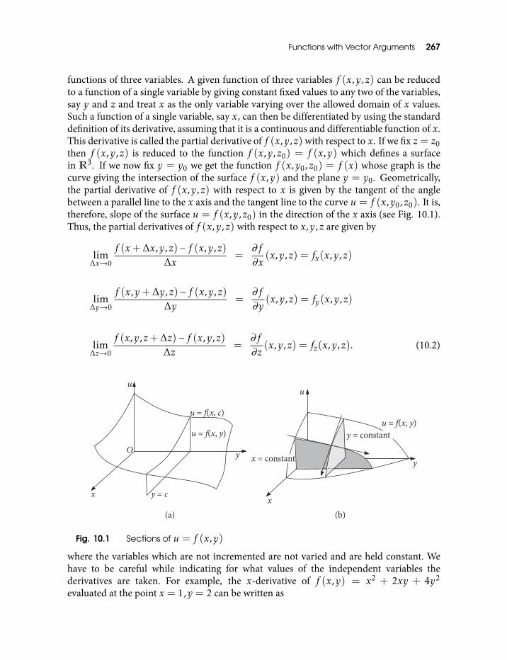
Functions with Vector Arguments 267
functions of three variables. A given function of three variables f (x,y,z) can be reducedto a function of a single variable by giving constant fixed values to any two of the variables,say y and z and treat x as the only variable varying over the allowed domain of x values.Such a function of a single variable, say x, can then be differentiated by using the standarddefinition of its derivative, assuming that it is a continuous and differentiable function of x.This derivative is called the partial derivative of f (x,y,z) with respect to x. If we fix z = z0then f (x,y,z) is reduced to the function f (x,y,z0) = f (x,y) which defines a surfacein R3. If we now fix y = y0 we get the function f (x,y0,z0) = f (x) whose graph is thecurve giving the intersection of the surface f (x,y) and the plane y = y0. Geometrically,the partial derivative of f (x,y,z) with respect to x is given by the tangent of the anglebetween a parallel line to the x axis and the tangent line to the curve u = f (x,y0,z0). It is,therefore, slope of the surface u = f (x,y,z0) in the direction of the x axis (see Fig. 10.1).Thus, the partial derivatives of f (x,y,z) with respect to x,y,z are given by
lim∆x→0
f (x+∆x,y,z)− f (x,y,z)∆x
=∂f
∂x(x,y,z) = fx(x,y,z)
lim∆y→0
f (x,y+∆y,z)− f (x,y,z)∆y
=∂f
∂y(x,y,z) = fy(x,y,z)
lim∆z→0
f (x,y,z+∆z)− f (x,y,z)∆z
=∂f
∂z(x,y,z) = fz(x,y,z). (10.2)
Fig. 10.1 Sections of u = f (x,y)
where the variables which are not incremented are not varied and are held constant. Wehave to be careful while indicating for what values of the independent variables thederivatives are taken. For example, the x-derivative of f (x,y) = x2 + 2xy + 4y2
evaluated at the point x = 1,y = 2 can be written as
268 An Introduction to Vectors, Vector Operators and Vector Analysis
(∂f (x,y)∂x
)x=1,y=2
= fx(1,2) = (2x+ 2y)x=1,y=2 = 6.
We should not write it simply as ∂f (1,2)∂x since f (1,2) = 21 is a constant and has 0 as its
x-derivative.Since the partial derivatives fx,y,z(x,y,z) are the functions of three variables, they can
be again partially differentiated with respect to x,y,z. Assuming that the order ofdifferentiation does not matter, we get the six derivatives, namely, fxx,fxy ,fxz,fyy ,fyz,fzz
where fxx =∂2f∂x2 =
∂fx∂x , fxy =
∂2f∂x∂y =
∂fy∂x etc.
Exercise Assuming that the order of differentiation does not matter, how many partialderivatives of order r of a function of n variables are possible?
Solution Let r1,r2, . . . ,rn denote the number of occurrences of the variables x1,x2, . . . ,xnin a rth order possible partial derivative of a function f (x1,x2, . . . ,xn). We must haver1 + r2 + · · ·+ rn = r . A general arrangement can be viewed as n stars separated by n− 1
bars. For example, the eighth order partial derivative of a six variable function ∂8f
∂x31∂x2∂x
46
corresponds to (r = 8 and n= 6) ∗ ∗ ∗| ∗ |||| ∗ ∗ ∗ ∗ where the string of stars ending at the kthbar (1 ≤ k ≤ n−1) gives the order of differentiation with respect to the variable xk and thestring of stars starting after the n−1th bar gives the order of differentiation with respect tothe variable xn. If a pair of bars does not sandwitch any stars, or if the last string of starsis absent, the differentiation with respect to the corresponding variable is absent. The totalnumber of distinct distributions is then given by the number of ways of selecting r placesout of n+ r − 1 places to be filled by stars and rest of the places are filled by bars. (thereare n+ r − 1 stars and bars together). This is given by (n+r−1
r ). Thus, there are (n+r−1r )
rth order partial derivatives of a function of n variables. A function of three variables hasfifteen derivatives of fourth order and 21 derivatives of fifth order.
In the last section we saw that the existence of the derivative of a function of a single scalarvariable guarantees the continuity of the function. In contrast to this, the existence of thepartial derivatives fx,y,z(x,y,z) does not imply the continuity of f (x,y,z). Thus forexample, the function u(x,y) = 2xy/(x2 + y2), (x,y) , (0,0) ; u(0,0) = 0 iscontinuous as a function of x for any fixed y and is also continuous as a function of y forany fixed x, so that it has partial derivatives everywhere. However, it is discontinuous at(0,0) as its value at all points on the line x = y is 1 except at (0,0). However, we have thefollowing results, which we state here without proof.
If a function f (x,y,z) has partial derivatives fx,fy and fz everywhere in an open setR and these derivatives everywhere satisfy the inequalities
|fx(x,y,z)| <M, |fy(x,y,z)| <M,
where M is independent of x,y,z then f (x,y,z) is continuous everywhere in R.
Functions with Vector Arguments 269
Further, if both the partial derivative of order r and the partial derivative obtained bychanging the order of differentiation in any way are continuous in a region R, then boththese derivatives are equal in R, that is, the order of differentiation is immaterial. Thismakes the number of partial derivatives of rth order of f (x,y,z) decidedly smaller thanotherwise expected, as we have calculated in the previous exercise.
10.3 Chain RuleConsider a function u(x,y,z) = u(ξ(x,y,z),η(x,y,z), . . .) to be a differentiable functionof n variables ξ,η, . . . each of which is a differentiable function of x,y,z. Let the functionsξ,η, . . . have as their common domain the region R in R3. All the n functions ξ,η, . . .together map a point inR to a point in the region S in Rn. The function u then maps thispoint to a scalar value. Thus, u is a differentiable function of x,y,z ; u : R3 7→ R. Thepartial derivatives of u with respect to x,y,z are then given by
ux =∂u∂ξ
∂ξ∂x
+∂u∂η
∂η
∂x+ · · ·= uξξx+ uηηx+ · · ·
uy =∂u∂ξ
∂ξ∂y
+∂u∂η
∂η
∂y+ · · ·= uξξy + uηηy + · · ·
uz =∂u∂ξ
∂ξ∂z
+∂u∂η
∂η
∂z+ · · ·= uξξz+ uηηz+ · · · (10.3)
Replacing x,y,z by x1,x2,x3 and ξ,η, . . . by ξ1,ξ2, . . . we can summarize the aboveequations by
uxk =n∑i=1
∂u∂ξi
∂ξi∂xk
k = 1,2,3. (10.4)
In order to prove Eq. (10.3) all that we need to use is that all functions involved aredifferentiable. We have,
ξ(x+∆x,y+∆y,z+∆z)−ξ(x,y,z) = ξ(x+∆x,y+∆y,z+∆z)−ξ(x,y+∆y,z+∆z)
+ξ(x,y+∆y,z+∆z)− ξ(x,y,z+∆z) + ξ(x,y,z+∆z)− ξ(x,y,z).
If we multiply three terms on RHS by ∆x∆x , ∆y
∆y and ∆z∆z respectively, we get an expression
linear in ∆x,∆y,∆z, that is,
270 An Introduction to Vectors, Vector Operators and Vector Analysis
∆ξ =ξ(x+∆x,y+∆y,z+∆z)− ξ(x,y+∆y,z+∆z)
∆x∆x
+ξ(x,y+∆y,z+∆z)− ξ(x,y,z+∆z)
∆y∆y
+ξ(x,y,z+∆z)− ξ(x,y,z)
∆z∆z. (10.5)
By differentiability of ξ(x,y,z) we mean that replacing the difference quotients on the RHSof this equation by the respective partial derivatives would give an error
• linear in the Euclidean distance traversed as we go from x,y,z to x+∆x,y+∆y,z+∆z, that is, the error is given by ερ, where ρ =
√∆x2 +∆y2 +∆z2 and
• the error goes to zero faster than ρ→ 0, that is, ε→ 0 faster than ρ→ 0.
Thus, we can write, upto first order of smallness in ρ, (That is, neglecting the terms ofthe second and higher order in ρ in the expression for error if any,)
∆ξ = ξx∆x+ ξy∆y+ ξz∆z.
This is exactly the same as replacing the distance traversed between two points along a pathby the Euclidean distance between these two points, a procedure we have incurred before.
Similarly, we get,
∆η = ηx∆x+ ηy∆y+ ηz∆z.
Since u is a differentiable function of ξ,η, . . . we can again write
∆u = uξ∆ξ + uη∆η+ · · ·
Substituting, the expressions for ∆ξ, ∆η · · · we get ∆u as a result of ∆x, ∆y ∆z as
∆u = (uξξx+ uηηx+ · · · )∆x+ (uξξy + uηηy + · · · )∆y+ (uξξz+ uηηz+ · · · )∆z.
However, considering u as a function of x,y,z we must have
∆u = ux∆x+ uy∆y+ uz∆z.
Comparing the last two equations for ∆u we get Eq. (10.3), which is called the chain rulefor differentiating a compound function of several variables.
Exercise Find expressions for all second order derivatives of u.
Exercise Find all partial derivatives of the first and the second order with respect to xand y for the following functions of x,y:
Functions with Vector Arguments 271
(i) u = v logw where v = x2 and w = 11+y .
(ii) u = evw, where v = ax and w = cosy.(iii) u = v tan−1w where v = xy
x−y and w = x2y+ y − x.
(iv) u = g(x2 + y2,ex−y).(v) u = tan(x tan−1 y).
10.4 Directional Derivative and the Grad OperatorAs we have seen above, for a function of three variables f (x) ≡ f (x,y,z) we can writeupto first order in ρ,
∆f = f (x+∆x)− f (x) =∂f
∂x∆x+
∂f
∂y∆y+
∂f
∂z∆z = ∇f ·∆x (10.6)
Equations (10.6), (10.7) define a new operator, called ‘grad’ or ‘del ’ operator whichoperates on a scalar valued function f (x) and returns a vector valued function (∇f )(x)via
(∇f )(x) =∂f
∂x(x)i+
∂f
∂y(x)j+
∂f
∂z(x)k. (10.7)
where i, j, k is the orthonormal basis in which coordinates of x are (x,y,z). Note that thenotation ∇(f (x)) is meaningless because f (x) is a number and the del operator does notact on a number.
In order to be useful, we must show that the definition of the del operator is invariantunder the change of basis, that is, it is the same for all orthonormal bases, so that the deloperator (∇f )(x) has the same value at x irrespective of the basis used to evaluate it. Wedo this by treating the del operator as a vector with coordinates u1 =
∂f∂x1
, u2 =∂f∂x2
,
u3 =∂f∂x3
with respect to the coordinate system corresponding to the basis i, j, k. Let thecoordinates of a vector x in this coordinate system be x1,x2,x3. We know that a newcoordinate system is obtained from the old one by rotating and/or translating it. Hence,the new coordinates say x′1,x′2,x′3 are related to the old ones by
x′j =3∑k=1
ajkxk + bj
where [ajk ] is an orthogonal matrix, whose inverse equals its transpose, and b is the vectorby which the origin of the old system is translated. Due to orthogonality of thetransformation [ajk ], the old coordinates can be re-expressed in terms of the new ones as
xk =3∑j=1
akj(x′j − bj), k = 1,2,3.
272 An Introduction to Vectors, Vector Operators and Vector Analysis
Under this coordinate transformation, a function f (x1,x2,x3) will get transformed to
g(x′1,x′2,x′3) so that the operator ∇f will get transformed to ∇f ≡(∂g∂x′1
, ∂g∂x′2
, ∂g∂x′3
). To
evaluate these partial derivatives we note that
g(x′1,x′2,x′3) = f
3∑k=1
ak1(x′k − bk),
3∑k=1
ak2(x′k − bk),
3∑k=1
ak3(x′k − bk)
.
Thus, the coordinates of ∇g with respect to the new coordinate system are given by
vj =∂g
∂x′j=
3∑k=1
∂f
∂xk
∂xk∂x′j
=3∑k=1
ajkuk .
where we have used the chain rule. Thus, under the coordinate transformation the operator∇f transforms like a vector and its components in the transformed system are given by thepartial derivatives of the transformed function with respect to the transformed coordinates.Given a vector x the vector (∇f )(x) is the same irrespective of the coordinate system usedto evaluate it.
We are now equipped to define the directional derivative of a function of three variables.Given a scalar valued function f (x) ≡ f (x,y,z), its derivative in a direction a is given by
(a · ∇)f = nx∂f
∂x+ ny
∂f
∂y+ nz
∂f
∂z(10.8)
where (nx,ny ,nz) are the direction cosines of a with respect to the basis i, j, k. This iscalled the directional derivative of f (x) in the direction a. Henceforth, we shall drop theparentheses in the expressions for the del operator and the directional derivative, implyingtheir actions implicitly. Also, we may allow replacing the unit vector a by a general vector a(with magnitude different than unity) in the definition of the directional derivative. In thatcase the direction cosines in Eq. (10.8) are replaced by the components of a.
Exercise Let f (x) ≡ f (x1,x2,x3) be a differentiable scalar valued function withx1,x2,x3 referring to the orthonormal basis i1, i2, i3. Show that ∂f
∂xk, k = 1,2,3 are the
directional derivatives along i1, i2, i3 respectively.
Solution Notice that ∂f∂xk
= ik ·∆f , k = 1,2,3.
Exercise Find the directional derivative of a scalar field f (x) along a continuous anddifferentiable curve parameterized by time t.
Answer This is simply the total time derivative of the function f (x(t)) with respect to tas can be seen from (see section 10.7)
df
dt= x · ∇f (x).
Functions with Vector Arguments 273
The RHS is just the directional derivative of f (x) in the direction of the velocity or thetangent vector to the curve.
The concept of the directional derivative can be quite simply generalized to vector fields asfollows. The directional derivative of a vector field f(x) ≡ (f1(x), f2(x), f3(x)) along a isgiven by a vector with components (a · ∇f1(x), a · ∇f2(x), a · ∇f3(x)) in the same basis inwhich the field f(x) is resolved. Since each component of ∇f is invarient under the changeof basis, so is ∇f itself.
Another elegant approach called geometric calculus is developed by D. Hestenes andcollaborators in the context of functions with multivector arguments. This approach canbe adapted to both the scalar as well as vector valued functions of vector arguments, vectorsbeing a special case of multivectors. This is a coordinate-free approach, where argumentsof functions are treated as vectors as such, without resolving them into components usinga particular basis. The increment ∆x in the vector argument x is decomposed as aτ wherethe vector a gives the direction and τ is a scalar variable. The directional derivative is thendefined as1
a · ∇f (x) = limτ→0
f (x+ aτ)− f (x)τ
. (10.9)
Note that this definition is meaningful even if the function f is vector valued, becausethe limit defining it is meaningful in that case. We will show below, for a scalar valuedfunction, that the definitions of the directional derivative given by Eqs (10.8) and (10.9) areequivalent. Thus, the LHS of Eq. (10.9) can be viewed as the dot product of a and ∇f (x).In this section, unless stated otherwise, the same symbol f will represent both the scalarand vector valued function and the corresponding result applies in both the cases.
We now obtain some basic results regarding the directional derivative. Consider
(a+b) · ∇f (x) = limτ→0
f (x+ aτ +bτ)− f (x)τ
= limτ→0
[f (x+ aτ +bτ)− f (x+ aτ)
τ+f (x+ aτ)− f (x)
τ
]
= a · ∇f (x) +b · ∇f (x). (10.10)
Similarly, for a scalar constant c,
(ca) · ∇f (x) = c limcτ→0
f (x+ cτa)− f (x)cτ
= c(a · ∇f (x)). (10.11)
Exercise Let f (x) and g(x) be two functions of vector argument x.
1See also ref [21]
274 An Introduction to Vectors, Vector Operators and Vector Analysis
(i) Show that
a · ∇(f + g) = a · ∇f + a · ∇g. (10.12)
(ii) Assuming either f or g or both to be scalar valued, or, by replacing the product f gby the dot product f · g if both are vector valued, show that
a · ∇(f g) = (a · ∇f )g + f (a · ∇g). (10.13)
We refer to this as the “product rule”. It is trivial to check that a ·∇cf (x) = ca ·∇f (x). Thisequation and Eq. (10.12) together show that the directional derivative is a linear operator.
Now let f be a scalar valued function of a scalar argument and let λ(x) be a scalarvalued function of a vector argument. Then, the directional derivative of the compoundfunction f (λ(x)) is
a · ∇f = limτ→0
[f (λ(x+ aτ))− f (λ(x))
λ(x+ aτ)−λ(x)λ(x+ aτ)−λ(x)
τ
]
=
[lim∆λ→0
f (λ+∆λ)− f (λ)∆λ
][limτ→0
λ(x+ aτ)−λ(x)τ
]
= (a · ∇λ)df
dλ. (10.14)
This is the chain rule for the directional derivative of a compound function.The directional derivative of the vector valued and the scalar valued constant functions
f(x) = b and f (x) = c are trivially zero, as seen from its definition. We have
a · ∇b = 0 = a · ∇c.
It follows directly from the definition of the directional derivative that the directionalderivative of the identity function I(x) = x is
a · ∇x = a.
We can use general rules Eqs (10.12) and (10.13) to find the derivatives of morecomplicated functions. The derivatives of algebraic functions of x can be obtained in thisway. For example, we note that the “magnitude function” |x| is related to x by the algebraicequation |x|2 = x · x. Using Eq. (10.13) we can write
a · ∇(x · x) = (a · ∇x) · x+ x · (a · ∇x) = a · x+ x · a = 2a · x. (10.15)
If we apply the chain rule (Eq. (10.14)) we get
a · ∇|x|2 = 2|x|a · ∇|x|.
Functions with Vector Arguments 275
Equating the RHS of both these equations we get
a · ∇|x|= a · x|x|
= a · x. (10.16)
Next, we find the derivative of the “direction function” x. We use the product rule(Eq. (10.13)) and the chain rule (Eq. (10.14)) as follows.
a · ∇( x|x|
)=
a · ∇x|x|− a · ∇|x||x|2
x =a|x|−(a · x)x|x|2
.
Hence,
a · ∇x =a− (a · x)x|x|
. (10.17)
Exercise Find the derivatives
(a) a · ∇(x×b) Where b is a constant vector independent of x.
Answer a×b. Follows from the definition of the directional derivative.
(b) a · ∇(x× (x×b)).
Answer (a ·b)x+ (x ·b)a− 2(a · x)b.
Hint Use identity I and the product rule.
Exercise Let r = r(x) = x−x′, r = |r|= |x−x′ | where x′ is independent of x. Show that(a) a · ∇r = a · r.
(b) a · ∇r =a− (a · r)r
r.
(c) a · ∇(r · a) =a2 − (a · r)2
r.
(d) a · ∇(r× a) =(a · r)(a× r)
r.
(e) a · ∇|r× a|2 = −(r · a)|r× a|
r.
(f) a · ∇ rr=
a− 2(a · r)rr2 .
(g) a · ∇ 1r2 = −2
a · rr3 .
(h)12(a · ∇)2 1
r2 =3(a · r)2 − |r× a|2
r4 .
(i)16(a · ∇)3 1
r2 = 4a · r(a · r)2 + |r× a|2
r5 .
276 An Introduction to Vectors, Vector Operators and Vector Analysis
(j) a · ∇ logr =a · rr
.
(k) a · ∇r2k = 2k(a · r)r2(k−1).
(l) a · ∇r2k+1 = r2k(a+ 2k(a · r)r).In the last two cases k , 0 is an integer and r , 0 if k < 0.
It is quite easy to see that the definition of the directional derivative in Eq. (10.8) followsfrom that in Eq. (10.9). Choosing an orthonormal basis e1, e2, e3 and denoting thecomponents of x with respect to this basis by x1,x2,x3 we get
a · ∇f (x) = (n1e1 + n2e2 + n3e3) · ∇f (x)
= n1e1 · ∇f (x) + n2e2 · ∇f (x) + n3e3 · ∇f (x)
= n1∂f
∂x1+ n2
∂f
∂x2+ n3
∂f
∂x3. (10.18)
The second equality follows from Eq. (10.10) and the last equality follows because thedirectional derivative (Eq. (10.9)) along the direction of one of the basis vectors reduces tothe corresponding partial derivative (Eq. (10.8)).
We note that the action of the ‘del ’ operator on a scalar valued function f (x) is thesame as that of the linear operator
∇ ≡3∑j=1
ej∂∂xj
= e1∂∂x1
+ e2∂∂x2
+ e3∂∂x3
. (10.19)
Using the linearity of the directional derivative and Eq. (10.18) we can express thedirectional derivative of a vector valued function in terms of the partial derivatives of itscomponent functions in an orthonormal basis (e1, e2, e3). We have,
a · ∇f(x) = a · ∇(f1(x)e1 + f2(x)e2 + f3(x)e3)
= a · ∇f1(x)e1 + a · ∇f2(x)e2 + a · ∇f3(x)e3
=
(n1∂f1∂x1
+ n2∂f1∂x2
+ n3∂f1∂x3
)e1 +
(n1∂f2∂x1
+ n2∂f2∂x2
+ n3∂f2∂x3
)e2
+
(n1∂f3∂x1
+ n2∂f3∂x2
+ n3∂f3∂x3
)e3. (10.20)
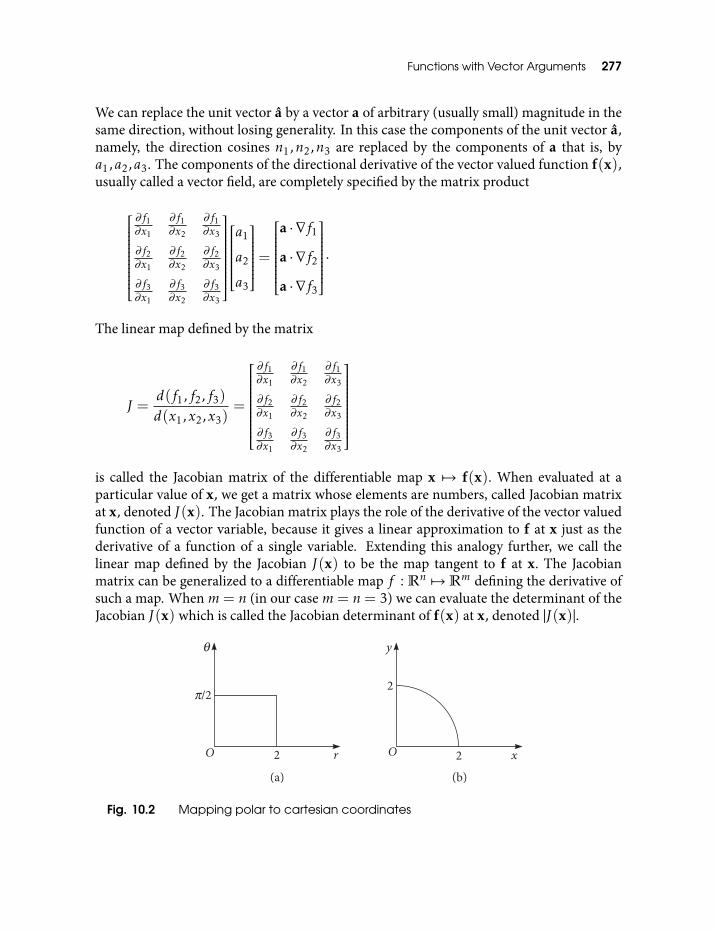
Functions with Vector Arguments 277
We can replace the unit vector a by a vector a of arbitrary (usually small) magnitude in thesame direction, without losing generality. In this case the components of the unit vector a,namely, the direction cosines n1,n2,n3 are replaced by the components of a that is, bya1,a2,a3. The components of the directional derivative of the vector valued function f(x),usually called a vector field, are completely specified by the matrix product
∂f1∂x1
∂f1∂x2
∂f1∂x3
∂f2∂x1
∂f2∂x2
∂f2∂x3
∂f3∂x1
∂f3∂x2
∂f3∂x3
a1
a2
a3
=a · ∇f1
a · ∇f2
a · ∇f3
·
The linear map defined by the matrix
J =d(f1,f2,f3)d(x1,x2,x3)
=
∂f1∂x1
∂f1∂x2
∂f1∂x3
∂f2∂x1
∂f2∂x2
∂f2∂x3
∂f3∂x1
∂f3∂x2
∂f3∂x3
is called the Jacobian matrix of the differentiable map x 7→ f(x). When evaluated at aparticular value of x, we get a matrix whose elements are numbers, called Jacobian matrixat x, denoted J(x). The Jacobian matrix plays the role of the derivative of the vector valuedfunction of a vector variable, because it gives a linear approximation to f at x just as thederivative of a function of a single variable. Extending this analogy further, we call thelinear map defined by the Jacobian J(x) to be the map tangent to f at x. The Jacobianmatrix can be generalized to a differentiable map f : Rn 7→ Rm defining the derivative ofsuch a map. Whenm= n (in our case m= n= 3) we can evaluate the determinant of theJacobian J(x) which is called the Jacobian determinant of f(x) at x, denoted |J(x)|.
Fig. 10.2 Mapping polar to cartesian coordinates
278 An Introduction to Vectors, Vector Operators and Vector Analysis
Exercise Let F : R2 7→R2 be the map defined by
F(r,θ) = (r cosθ,r sinθ) r ≥ 0
In other words, the polar coordinates map (r,θ) 7→ (x,y) as
x = r cosθ, y = r sinθ
which maps a rectangle into a circular sector (see Fig. 10.2). Find the Jacobian matrix andthe Jacobian determinant of this mapping. Find all points (r,θ) where the Jacobiandeterminant vanishes.
10.5 Taylor SeriesWe can extend the Taylor series approximation to the functions of vector argument. Thisenables us to approximate the arbitrary functions of vectors (mostly position vectors) bysimpler functions. Such a Taylor series involves directional derivatives, and applies tofunctions for which directional derivatives (or, equivalently, partial derivatives) of allorders (see below) exist. The basic idea is to use the Taylor series expansion of thefunction with scalar argument. Given a scalar or vector valued function f (x) to beapproximated, we invoke a new function of scalar argument
G(τ) = f (x+ aτ).
Using this definition of G(τ) and the definition of the directional derivative (Eq. (10.9)) itis clear that
dG(0)dτ
= a · ∇f (x),
d2G(0)dτ2 = a · ∇(a · ∇f (x)) ≡ (a · ∇)2f (x),
dkG(0)dτk
= a · ∇((a · ∇)k−1f (x)) = (a · ∇)kf (x). (10.21)
We now expand the function with scalar argument G(τ) in Taylor series about τ = 0 andevaluate it at τ = 1. We get
G(1) = G(0) +dG(0)dτ
+12d2G(0)dτ2 + · · ·=
∞∑k=0
1k!dkG(0)dτk
.
Functions with Vector Arguments 279
Using Eq. (10.21) we can express this Taylor series in terms of f (x). This gives the desiredTaylor expansion
f (x+ a) = f (x) + a · ∇f (x) +(a · ∇)2
2!f (x) + · · ·
=∞∑k=0
(a · ∇)k
k!f (x) ≡ ea·∇f (x), (10.22)
where the last equivalence defines the operator ea·∇.If f is a vector valued function f(x)we can resolve it in terms of its component functions
with respect to some orthonormal basis and use Eq. (10.20) iteratively to get the Taylorexpansion
f(x+ a) =
f1(x)
f2(x)
f3(x)
+a · ∇f1(x)
a · ∇f2(x)
a · ∇f3(x)
+12!
(a · ∇)2f1(x)
(a · ∇)2f2(x)
(a · ∇)2f3(x)
+ · · ·Each element in the second term is simply the dot product of a and ∇fk(x), k = 1,2,3.The second term is given by the product of the Jacobian matrix and the vectora↔ [a1a2a3]
T .
10.6 The DifferentialThe general form of the remainder after two terms in the Taylor series of a scalar valuedfunction f (x) can be found by the following argument. We say that f (x) is differentiableat x if all its partial derivatives exist at x, or, the vector ∇f (x) is well defined. Since wecannot divide by a vector increment ∆x we can re-write the Newtonian quotient as
df = f (x+∆x)− f (x) = ∆x · ∇f (x) + |∆x|g(∆x) (10.23)
such that g(∆x) → 0 as |∆x| → 0. Note that the first term on RHS is simply thedirectional derivative in the direction of ∆x. This equation implies that, for any requiredaccuracy, we can choose |a| small enough so as to make the first two terms of the Taylorseries in Eq. (10.22) give the value of f (x + a) within the required accuracy. In otherwords, the remainder term in the series obtained after truncating it after the second term,namely the last term in the equation
f (x+ a) = f (x) + a · ∇f (x) + |a|g(a) (10.24)
280 An Introduction to Vectors, Vector Operators and Vector Analysis
can be chosen as small as we please by choosing |a| small enough.2 We call the directionalderivative appearing in this equation, namely, a · ∇f (x), the differential of the functionf (x). For a scalar valued function, f (x), Eq. (10.23) is the equation for a line in 3-D inthe range x and x+dx. Thus, we see that, for any scalar valued differentiable function, thedifferential provides a linear approximation to that function in a small enough range of itsargument. For a vector valued function f(x) Eq. (10.24) now becomes a vector equation,with f replaced by
f(x+ a) =
f1(x)
f2(x)
f1(x)
+a · ∇f1(x)
a · ∇f2(x)
a · ∇f3(x)
+ |a|g1(a)
g1(a)
g1(a)
,
where the scalar valued functions fk(x), k = 1,2,3 are the components of f(x) withrespect to some orthonormal basis. The term in the middle, involving the gradients, isprecisely equal to the product of the Jacobian matrix times a ≡ [a1a2a3]
T . Sincelim|a|→0 gk(a) = 0; k = 1,2,3 we can make the linear approximation to f(x) at x by theJacobian matrix J(x) as accurate as we please by making |a| small enough.
To appreciate the importance of the differential, (which is the same as the directionalderivative of a scalar valued or vector valued function f (x) in the direction of fixed vector(a), we view it as a function of a for fixed x, say F(a). We have already shown that thedifferential is a linear function of a (see Eqs (10.10),(10.11)). Expanding the Taylor seriesabout the point x0 and putting ∆x = x− x0 we have, for small enough |∆x|,
f (x0 +∆x) = f (x) = f (x0) +∆x · ∇f (x0) = (x− x0) · ∇f (x0). (10.25)
Note that the vector x−x0 in the differential (x−x0) · ∇f (x0) plays the role of vector a ina · ∇f (x) which is a linear function of a. Therefore, using this linearity and Eq. (10.25) weget, to the first order in ∆x
f (x)−f (x0) = (x−x0) ·∇f (x0) = x·∇f (x0)−x0 ·∇f (x0) = F(x)−F(x0). (10.26)
If we couple linearity of F(x) with Eq. (10.26), we see that the differential provides a linearapproximation to any differentiable function. Since linear functions are simple enough tobe analyzed completely, Eq. (10.26) establishes the importance of the differential. Notethat Eqs (10.25) and (10.26) apply to both the scalar valued as well as the vector valuedfunction f (x).
2Compare with
f (a+ h) = f (a) +df
dx
∣∣∣∣x=a
h+ |h|g(h)
where
limh→0
g(h) = 0.
Functions with Vector Arguments 281
10.7 Variation on a CurveWe are often interested in the variation of a function f (x) along the path of a movingparticle parametrically given by x = x(t). Let us first assume that f (x) is scalar valued.We know that the general variation of such a function is given by
f (x+∆x) = f (x) +∆x · ∇f (x).
However, both x and ∆x are now not arbitrary, but x must satisfy x = x(t) and ∆x mustjoin the point x(t) and a neighboring point on the path given by x(t + ∆t), that is,∆x = x(t+∆t)− x(t). Therefore, the variation of f (x) along the curve is given by
f (x(t+∆t)) = f (x(t)) + (x(t+∆t)− x(t)) · ∇f (x(t)).
Now we subtract f (x(t)) from both sides, divide by ∆t on both sides and take the limit as∆t→ 0 on both sides to get the desired result,
df
dt(x(t)) = x(t) · ∇f (x(t)) =
3∑i=1
xi(t)∂f
∂xi, (10.27)
where xi i = 1,2,3 and xi i = 1,2,3 are the components of x(t) and x(t) respectively,with respect to some orthonormal basis. Thus, the time rate of change of a function of theposition vector of a particle, as it moves along its path, is given by the directional derivativeof this function along the direction of the velocity vector, which is tangent to the path inthe same sense as traversed by the particle.
Exercise The Lagrangian of a system with n degrees of freedom is a function of 2n+ 1variables, namely, L (q(t); q(t); t) where q(t) ≡ q1(t),q2(t), . . . ,qn(t) are thegeneralized coordinates and q(t) ≡ q1(t), q2(t), . . . , qn(t) are the generalized velocities.The motion is viewed as the path traced by a point in the configuration space spanned bythe n generalized coordinates. Similarly, the Hamiltonian of such a system is given as afunction of 2n+ 1 coordinates, namely, H (q(t);p(t); t) where p(t) ≡ p1,p2, . . . ,pn arethe generalized momenta. The motion is viewed as that of a point in phase space spannedby n generalized coordinates and n generalized momenta. Find the expressions for dL
dt
and dHdt .
Answer
dLdt
=n∑i=1
∂L∂qi
qi +n∑i=1
∂L∂qi
qi +∂L∂t
,
where qi =ddt qi .
dHdt
=n∑i=1
∂H∂qi
qi(p(t)) +n∑i=1
∂H∂pi
pi +∂H∂t
,
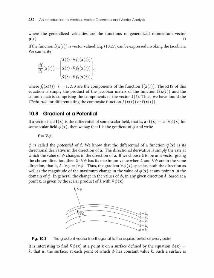
282 An Introduction to Vectors, Vector Operators and Vector Analysis
where the generalized velocities are the functions of generalized momentum vectorp(t).
If the function f(x(t)) is vector valued, Eq. (10.27) can be expressed invoking the Jacobian.We can write
dfdt
(x(t)) =
x(t) · ∇f1(x(t))
x(t) · ∇f2(x(t))
x(t) · ∇f3(x(t))
,
where fi(x(t)) i = 1,2,3 are the components of the function f(x(t)). The RHS of thisequation is simply the product of the Jacobian matrix of the function f(x(t)) and thecolumn matrix comprising the components of the vector x(t). Thus, we have found theChain rule for differentiating the composite function f (x(t)) or f(x(t)).
10.8 Gradient of a PotentialIf a vector field f(x) is the differential of some scalar field, that is, a · f(x) = a · ∇φ(x) forsome scalar field φ(x), then we say that f is the gradient of φ and write
f = ∇φ.
φ is called the potential of f. We know that the differential of a function φ(x) is itsdirectional derivative in the direction of a. The directional derivative is simply the rate atwhich the value of φ changes in the direction of a. If we choose a to be unit vector givingthe chosen direction, then a · ∇φ has its maximum value when a and ∇φ are in the samedirection, that is, a · ∇φ = |∇φ|. Thus, the gradient ∇φ(x) specifies both the direction aswell as the magnitude of the maximum change in the value of φ(x) at any point x in thedomain of φ. In general, the change in the values of φ, in any given direction a, based at apoint x, is given by the scalar product of a with ∇φ(x).
Fig. 10.3 The gradient vector is orthogonal to the equipotential at every point
It is interesting to find ∇φ(x) at a point x on a surface defined by the equation φ(x) =k, that is, the surface, at each point of which φ has constant value k. Such a surface is
Functions with Vector Arguments 283
called an equipotential surface. Actually, the equation φ(x) = k defines a one-parameterfamily of equipotential surfaces, one surface for each constant value of k (see Fig. 10.3).At any point x on an equipotential surface the vector ∇φ(x) cannot have a componenttangential to the surface because a non-zero gradient tangential to the surface would meanthat φ(x) changes as x changes along the surface, contradicting the equipotential nature ofthe surface. Thus, at every point x on an equipotential surface the vector ∇φ(x) must benormal to the surface through that point. Further, it is directed towards the surfaces withlarger values of k, because the sign of the directional derivative is the same as that of thedifference in φ values and in the present case, the sign of the directional derivative is thesame as that of ∇φ(x). Figure 10.3 shows only a two dimensional cross section. In thisfigure, the change in k is the same for each pair of neighboring surfaces, so the separationprovides a measure of the change in φ. The closer the surfaces, larger the gradient.
Given a scalar valued function φ(x) its gradient at x is easily found by evaluating thecorresponding directional derivative a · ∇φ(x) which is simply the scalar product of ∇φwith an arbitrary vector a. Thus, for φ(x) = x · b where b is a constant vector, we geta · ∇(x ·b) = a ·b which follows from a · ∇x = a. Hence,
∇x ·b = b.
Similarly, from Eqs (10.15) and (10.16) we get
∇x2 = 2x,
∇|x| = x. (10.28)
These formulas enable us to determine the gradients of certain functions without referringto the directional derivative at all. Thus, if f (|x|) is a function of the magnitude of x alone,then, by using the second of Eq. (10.28) while applying the chain rule Eq. (10.14), we get
∇f = x∂f
∂|x|· (10.29)
Later we will meet potential functions in connection with the line integrals over vectorfields derivable from a potential.
10.9 Inverse Maps and Implicit FunctionsWe have already seen the conditions for the map f : E3 7→ E3 to be invertible(subsection 4.1.2). Here, we are interested in a class of maps (or functions) which aredifferentiable, called C1 functions, so we define the inverse of a function over the set of C1
functions. Further, by E3 we mean E3 or R3. Let U denote some open set in E3. A mapf : U 7→ E3 is called a C1-map on U if a · ∇f and (a · ∇)2f exist at all x ∈ U and for all a.This is equivalent to saying that all partial derivatives of all the component functionsf1(x),f2(x),f3(x) of f(x) exist and are continuous at all x ∈ U . A C1-map f : U 7→ E3 is
284 An Introduction to Vectors, Vector Operators and Vector Analysis
said to be C1-invertible if the image set f(U ) is an open set V and if there exists a C1-mapg : V 7→ U such that g f and f g are the respective identity maps on U and V . Forexample, if f : E3 7→ E3 is given by f(x) = x + b where b is a fixed vector, then f isC1-invertible, its inverse being the translation by −b.
Exercise LetU be the subset of R2 consisting of all pairs (r,θ) with r > 0 and 0 < θ < π.Let
f(r i+θj) = r cosθi+ r sinθj, (10.30)
with x = r cosθ and y = r sinθ. Show that this is a C1-map and find the image set f(U ).Show that the inverse map is given by
g(xi+ y j) =√x2 + y2i+ cos−1 x√
x2 + y2j,
with r =√x2 + y2 and θ = cos−1 x√
x2+y2.
Answer The image of U is the upper half plane consisting of all (x,y) such that y > 0,and arbitrary x. Inverse can be checked explicitly.
In many cases a map may not be invertible over the whole space or over arbitrary subsetsof it, but can still be C1-invertible locally in the following sense. Let a point x ∈ U . We saythat a map f is locally C1-invertible at x if there exists an open setU1 satisfying x ∈U1 ⊂Usuch that f is C1-invertible onU1.
Exercise Show that the map given by Eq. (10.30) is not C1-invertible on all of R2, butgiven any point, it is locally invertible at that point.
Hint If we take r < 0, the inverse map given in the previous exercise does not work.However, we can locally invert by choosing r = −
√x2 + y2 in the inverse map at a point
with r < 0.
In most cases the locally invertible map cannot be expressed in closed form. However, thereis a very important result which gives computable criterion for local invertibility of a map.
10.9.1 Inverse mapping theorem
Let U be an open set in E3 and f : U 7→ E3 be a C1 map. Let x be a point in U . If theJacobian determinant |jf(x)| , 0 then f is locally C1-invertible at x.
We do not give a formal proof of this theorem which is quite involved. However, wenote that the Jacobian matrix corresponding to a vector valued map f(x) plays the role ofits derivative at x. The Jacobian matrix itself is a linear map a 7→ a·∇f giving the directionalderivative of f along a. The determinant |Jf(x)| , 0 means that the the Jacobian matrix isinvertible at x. Thus, the inverse mapping theorem states that the map f is locally invertibleat x if the linear map defining its derivative, namely, its Jacobian matrix is invertible at x.
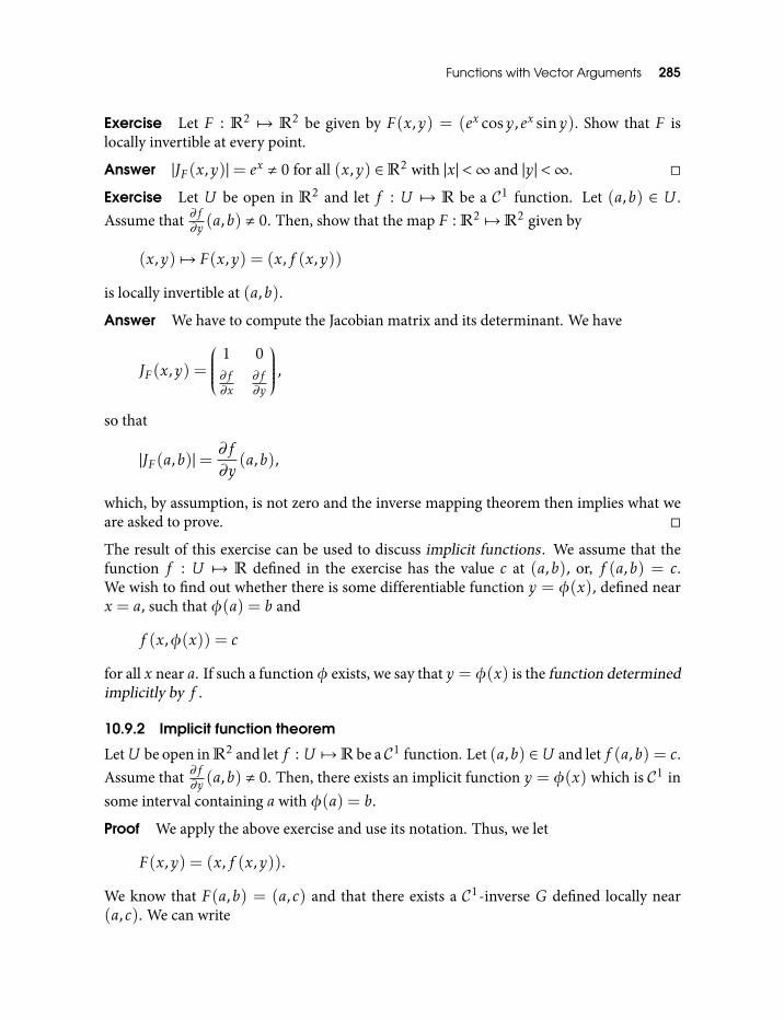
Functions with Vector Arguments 285
Exercise Let F : R2 7→ R2 be given by F(x,y) = (ex cosy,ex siny). Show that F islocally invertible at every point.
Answer |JF(x,y)|= ex , 0 for all (x,y) ∈R2 with |x| <∞ and |y| <∞.
Exercise Let U be open in R2 and let f : U 7→ R be a C1 function. Let (a,b) ∈ U .Assume that ∂f∂y (a,b) , 0. Then, show that the map F : R2 7→R2 given by
(x,y) 7→ F(x,y) = (x,f (x,y))
is locally invertible at (a,b).
Answer We have to compute the Jacobian matrix and its determinant. We have
JF(x,y) =
1 0∂f∂x
∂f∂y
,
so that
|JF(a,b)|=∂f
∂y(a,b),
which, by assumption, is not zero and the inverse mapping theorem then implies what weare asked to prove.
The result of this exercise can be used to discuss implicit functions . We assume that thefunction f : U 7→ R defined in the exercise has the value c at (a,b), or, f (a,b) = c.We wish to find out whether there is some differentiable function y = φ(x), defined nearx = a, such that φ(a) = b and
f (x,φ(x)) = c
for all x near a. If such a functionφ exists, we say that y = φ(x) is the function determinedimplicitly by f .
10.9.2 Implicit function theorem
LetU be open in R2 and let f : U 7→R be a C1 function. Let (a,b) ∈U and let f (a,b) = c.Assume that ∂f∂y (a,b) , 0. Then, there exists an implicit function y = φ(x) which is C1 insome interval containing a with φ(a) = b.
Proof We apply the above exercise and use its notation. Thus, we let
F(x,y) = (x,f (x,y)).
We know that F(a,b) = (a,c) and that there exists a C1-inverse G defined locally near(a,c). We can write
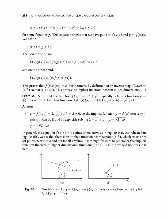
286 An Introduction to Vectors, Vector Operators and Vector Analysis
G(x,f (x,y)) = G(x,z) = (x,y) = (x,g(x,z))
for some function g . This equation shows that we have put z = f (x,y) and y = g(x,z).We define
φ(x) = g(x,c).
Then on the one hand,
F(x,φ(x)) = F(x,g(x,c)) = F(G(x,c)) = (x,c)
and on the other hand,
F(x,φ(x)) = (x,f (x,φ(x))).
This proves that f (x,φ(x)) = c. Furthermore, by definition of an inverse map, G(a,c) =(a,b) so that φ(a) = b. This proves the implicit function theorem in two dimensions.
Exercise Show that the function f (x,y) = x2 + y2 implicitly defines a function y =φ(x) near x = 1. Find this function. Take (i) (a,b) = (1,1), (ii) (a,b) = (−1,−1).
Answer
(i) c = f (1,1) = 2. ∂f∂y (1,1) = 2 , 0, so the implicit function y = φ(x) near x = 1
exists. It can be found by explicitly solving 2 = x2 + y2 : y =√
2− x2.
(ii) y = −√
2− x2.
In general, the equation f (x,y) = c defines some curve as in Fig. 10.4(a). As indicated inFig. 10.4(b), we see that there is an implicit function near the point (a,b), which exists onlyfor points near x = a and not for all x values. It is straightforward to generalize the implicitfunction theorem to higher dimensional functions f : Rn 7→ R but we will not pursue ithere.
Fig. 10.4 Neighborhood of point (a,b) on f (x,y) = c is locally given by the implicitfunction y = f (x)
Functions with Vector Arguments 287
10.9.3 Algorithm to construct the inverse of a map
We give an iterative algorithm [5], using the method of successive approximations, toconstruct the inverse of the locally C1-invertible map f : E3 7→ E3
u = f(x) = u(x)i+ v(x)j+w(x)k
with
u(x) = φ(x,y,z), v(x) = ψ(x,y,z), w(x) = χ(x,y,z).
That is, we want to solve the equation u = f(x) for x where u is a point near u0 = f(x0),where, at x = x0 we must have, for the Jacobian determinant |Jf(x0)|,
|Jf(x0)|=
∣∣∣∣∣∣∣∣∣∣∣φx(x0) φy(x0) φz(x0)
ψx(x0) ψy(x0) ψz(x0)
χx(x0) χy(x0) χz(x0)
∣∣∣∣∣∣∣∣∣∣∣ , 0.
The differentials dx,dy,dz and du,dv,dw satisfy the linear relations (see Eq. (10.23))
du = dφ = φxdx+φydy+φzdz
dv = dψ = ψxdx+ψydy+ψzdz
dw = dχ = χxdx+χydy+χzdz (10.31)
or,du = Jf(x)dx (10.32)
where
Jf(x) =
φx(x) φy(x) φz(x)
ψx(x) ψy(x) ψz(x)
χx(x) χy(x) χz(x)
is the Jacobian giving the derivative of the map u = f(x).
Exercise Find an upper bound on the Euclidean distance of the images of the points xand x+∆x under the map f : E3 7→ E3.
Solution The required distance is given by (see Equation following Eq. (10.24) and notethat ∆x · ∇f (x) is a vector),√
(f(x+∆x)− f(x)) · (f(x+∆x)− f(x)) =√(∆x · ∇f (x)) · (∆x · ∇f (x))
288 An Introduction to Vectors, Vector Operators and Vector Analysis
or, √(∆x · ∇f (x)) · (∆x · ∇f (x))
=√(hφx+ kφy + lφz)2 + (hψx+ kψy + lψz)2 + (hχx+ kχy + lχz)2 (10.33)
where φx,y,z,ψx,y,z,χx,y,z are the partial derivatives giving the row-wise elements of theJacobian matrix and h,k, l are the components of ∆x. LetM denote an upper bound on theabsolute values of all the elements of the Jacobian matrix taken at all points of the segmentjoining x and x+∆x. This gives√
(hφx+ kφy + lφz)2 + (hψx+ kψy + lψz)2 + (hχx+ kχy + lχz)2
≤√
3M(|h|+ |k|+ |l|) ≤ 3M√h2 + k2 + l2 (10.34)
which is the required upper bound.
Thus, the distance of the image points is at most 3M times that of the original ones. Writingy = x+∆x we can write Eq. (10.34) as
|f(y)− f(x)| ≤ 3M |y− x|. (10.35)
We now consider the mapping u = f(x) in a neighborhood
|x− x0| < δ (10.36)
of the point x0 in the domainR of f. Let u0 = f(x0). For a fixed u we write the equationu = f(x) which is to be solved for x, in the form
x = g(x), (10.37)
where
g(x) = x+A(u− f(x)); (10.38)
where A stands for an appropriately chosen fixed non-singular operator (or matrix) withinverse denoted by A−1. Thus, Eq. (10.37) is equivalent to A(u − f(x)) = 0, which bymultiplication with A−1 yields
A−1A(u− f(x)) = I(u− f(x)) = (u− f(x)) = 0,
where I is the identity operator represented by the unit matrix. Thus, a solution x ofEq. (10.37), that is, a fixed point of the map g, furnishes a solution of u = f(x).
Functions with Vector Arguments 289
We show that a fixed point of the map g can be reached by reaching the limit of xndefined by the recursion formula
xn+1 = g(xn) n= 0,1,2, . . . (10.39)
provided the Jacobian matrix, which in this case we denote by g′(x), representing thederivative of the vector mapping g is of sufficiently small size. This procedure is popularlyknown as the method of successive approximations. Making the ‘small size’ requirementmore precise, we require that for all x in the neighborhood of x0 given by Eq. (10.36), thelargest element of the matrix g′ is less than 1
6 in absolute value and that
|g(x0)− x0| <12δ.
The last equation is the condition on the initial value from which to start the iteration.First, we prove by induction that, under the assumptions stated, the recursion formula
in Eq. (10.39) successively gives vectors satisfying Eq. (10.36). This assures us that xn lie inthe domain of g so that the sequence can be continued indefinitely. From Eq. (10.35) withM = 1
6 we see that,
|g(y)− g(x)| ≤ 12|y− x| for |x− x0| < δ, |y− x0| < δ. (10.40)
Now the inequality in Eq. (10.36) holds trivially for x = x0. If it holds for x = xn, we findfor the vector xn+1 defined by Eq. (10.39) that
|xn+1−x0| ≤ |xn+1−x1|+ |x1−x0|= |g(xn)−g(x0)|+ |g(x0)−x0| ≤12|xn−x0|+
12δ.
This proves that |xn − x0| < δ for all n.To see that the sequence xn converges, we observe that by Eq. (10.40),
|xn+1 − xn|= |g(xn)− g(xn−1)| ≤12|xn − xn−1|.
In the same way,
|xn − xn−1| ≤12|xn−1 − xn−2|,
|xn−1 − xn−2| ≤12|xn−2 − xn−3|
and so on. These inequalities together imply
|xn+1 − xn| ≤12n|x1 − x0| ≤
δ
2n+1 . (10.41)
290 An Introduction to Vectors, Vector Operators and Vector Analysis
Since the distance between successive iterates decreases exponentially, the sequence xnmust converge to its limit say x∗. In this limit, the distance between successive iterates goesto zero. Therefore, the substitution of this limit x∗ in g(x) must return the same vector x∗.In other words this limit x∗ solves Eq. (10.37). Another way to see this is the following.Since g(x) is continuous, if the sequence xk k = 1,2, . . . converges to x∗ the sequenceg(xk) k = 1,2, . . . must converge to g(x∗). However, by virtue of Eq. (10.39) these twosequences are identical, making their limits the same, that is, x∗ = g(x∗).
Since the function g depends continuously on u, the xn obtained successively byrecursion formula Eq. (10.37) also depends continuously on u. Since the convergence ofthe sequence xn does not depend on u, it follows that its limit x∗ is a continuousfunction of u. Also, we have |x∗ − x0| ≤ δ because |xn − x∗| < δ for all n. If there existed asecond solution x′ with x′ = g(x′) and |x′ − x0| ≤ δ we find from Eq. (10.40) that
|x′ − x∗|= |g(x′)− g(x∗)| ≤ 12|x′ − x∗|
which makes |x′ − x∗|= 0 and x′ = x∗.Thus, we have established the existence, uniqueness and continuity of a solution x∗ of
the equation u = f(x), for which |x∗ − x0| ≤ δ, provided the function g(x) defined byEq. (10.38) has the derivative g′ with elements less than 1
6 in absolute value for|x∗ − x0| ≤ δ and provided |g(x0) − x0| < 1
2δ. These requirements can be satisfied for all usufficiently close to u0 by a suitable choice of the matrix A. By the definition of g(Eq. (10.38))
g′(x) = I −Af′(x),
where I is the identity. Then, for x = x0
g′(x0) = I −Af′(x0) = 0
if we choose for A the inverse of the matrix f′(x0), that is,
A= (f′(x0))−1.
The existence of this inverse is guaranteed by our basic assumption that the matrix f′(x0)has a non-vanishing determinant, that is, the Jacobian of the mapping f does not vanish atthe point x0. The assumed continuity of the first derivatives of the mapping f implies thatg′(x) depends continuously on x; hence the the elements of g′(x) are arbitrarily small, forinstance less than 1
6 , for sufficiently small |x − x0|, say for |x − x0| ≤ δ. Moreover, byEq. (10.38)
|g(x0)− x0|= |A(u− f(x0))|= |A(u−u0| <12δ,
Functions with Vector Arguments 291
provided u lies in a sufficiently small neighborhood of u0. This completes the proof ofthe local existence of a continuous inverse for a continuously differentiable mapping withnon-vanishing Jacobian.
The existence of the inverse of the Jacobian of the map u = f(x) at a point x can beused to show the continuity and differentiability of the inverse map x = f−1(u). Since theJacobian defines a linear, continuous and invertible map at x it must be one-to-one andonto on some neighborhood of x. Furthermore, every point v , u in this neighborhood,is given by v = f(y), y , x. This means that as v→ u through some sequence of points,y→ x. This enables us to invert the differential of f(x) in the following way.
f(y)− f(x) = v−u = J(x) · (y− x) + |y− x|h(y− x),
or,
y− x = J−1(x)(v−u) + |v−u|ε(v−u),
where
limv→u
ε(v−u) = 0.
This equation just says that the vector x satisfying u = f(x) is a differentiable function ofvector u and that the Jacobian matrix of x with respect to u is the inverse of the matrixf′(x) = J(x).
10.10 Differentiating Inverse FunctionsLet f(x) be a differentiable and invertible function. We assume the differentiability of theinverse function. Let the components of f(x) be 3
u = φ(x,y,z) v = ψ(x,y,z) w = χ(x,y,z),
and the components of the inverse be
x = g(u,v,w) y = h(u,v,w) z = k(u,v,w).
We substitute the inverse functions in the given functions to get the compound functions
φ(g(u,v,w),h(u,v,w),k(u,v,w)), ψ(g(u,v,w),h(u,v,w),k(u,v,w)),
χ(g(u,v,w),h(u,v,w),k(u,v,w)),
3The transformation f(x) could be passive, that is, the one which changes the coordinates of the same vector referring to adifferent basis.
292 An Introduction to Vectors, Vector Operators and Vector Analysis
which must be equal to u v and w respectively. Thus, we get the equations
u = φ(g(u,v,w),h(u,v,w),k(u,v,w))
v = ψ(g(u,v,w),h(u,v,w),k(u,v,w))
w = χ(g(u,v,w),h(u,v,w),k(u,v,w)) (10.42)
These equations are identities as they hold for all values of u,v,w. We now differentiateeach of these equations with respect to u v and w regarding them as independentvariables and apply the chain rule to differentiate the compound functions. We thenobtain the system of equations
1 = φxgu +φyhu +φzku 0 = φxgv +φyhv +φzkv 0 = φxgw+φyhw+φzkw
0 = ψxgu +ψyhu +ψzku 1 = ψxgv +ψyhv +ψzkv 0 = φxgw+φyhw+φzkw
0 = χxgu +χyhu +χzku 0 = χxgv +χyhv +χzkv 1 = χxgw+χyhw+χzkw
Solving these equations for nine unknowns gu,v,w,hu,v,w,ku,v,w we get the partialderivatives of the inverse functions x = g(u,v,w), y = h(u,v,w), z = k(u,v,w) withrespect to u,v,w expressed in terms of the derivatives of the original functions φ(x,y,z),ψ(x,y,z),χ(x,y,z) with respect to x,y,z, namely,
gu =1D[ψyχz −ψzχy ] gv =
1D[χyφz −χzφy ] gw
=1D[φyψz −φzψy ]
hu =1D[ψzχx −ψxχz] hv =
1D[χzφx −χxφz] hw
=1D[φzψx −φxψz]
ku =1D[ψxχy −ψyχx] kv =
1D[χxφy −χyφx] kw
=1D[φxψy −φyψx] (10.43)
Functions with Vector Arguments 293
where D stands for the Jacobian determinant
|Jf(x)|= D =
∣∣∣∣∣∣∣∣∣∣φx φy φz
ψx ψy ψz
χx χy χz
∣∣∣∣∣∣∣∣∣∣ ·This justifies calling the Jacobian the derivative of a differentiable map f : E3 7→ E3. For a2-D map Eq. (10.43) reduce to
gu =ψyD
, gv = −φyD
, hu = −ψxD
, hv =φxD
, (10.44)
where the Jacobian determinant D is given by
D =
∣∣∣∣∣∣φx φyψx ψy
∣∣∣∣∣∣ ·Exercise For polar coordinates in the plane expressed in terms of rectangularcoordinates,
u = r =√x2 + y2, v = θ = tan−1 y
x,
find the partial derivatives rx,ry ,θx,θy and the Jacobian determinant.
Solution The partial derivatives are
rx =x√
x2 + y2=xr
, ry =y√
x2 + y2=y
r,
θx =−y
x2 + y2 = −y
r2 , θy =x
x2 + y2 =x
r2 . (10.45)
Hence, the Jacobian has the value
D =xrx
r2 −y
r
(−y
r2
)=
1r
and the partial derivatives of the inverse functions (cartesian coordinates expressed interms of polar coordinates) are
xr =xr
, xθ = −y, yr =y
r, yθ = x,
as we could have found by direct differentiation of the inverse formulae x = r cosθ,y =r sinθ.
294 An Introduction to Vectors, Vector Operators and Vector Analysis
From the formulae for the derivatives of the inverse functions (Eq. (10.44)) for the 2-D case,we find that the Jacobian determinant of the functions x = x(u,v) and y = y(u,v) (wherethe coordinates themselves replace the function names g and h) with respect to u and visgiven by
d(x,y)d(u,v)
= xuyv − xvyu =uxvy −uyvx
D2 =1D
=
(d(u,v)d(x,y)
)−1
. (10.46)
Thus, the Jacobian determinant of the inverse system of functions is the reciprocal of theJacobian determinant of the original system.4 This is not surprising, because theseJacobians are the inverses of each other, as we have shown above (see the last para beforethe present subsection).
Exercise Find the second order derivatives for a 2-D map xuu = ∂2x∂u2 = guu and yuu =
∂2y∂u2 = huu .
Hint Differentiate the equations (with ux = φx, xu = gu etc.)
1 = uxxu + uyyu
0 = vxxu + vyyu (10.47)
again with respect to u and use the chain rule. Then, solve the resulting system of linearequations regarding the quantities xuu and yuu as unknowns and then replace xu and yuby the expressions already known for them. Note that the determinant of the doublydifferentiated system is again D and hence, by hypothesis, is not zero.
Answer
xuu = −1D3
∣∣∣∣∣∣∣uxxv2y − 2uxyvxvy + uyyv2
x uy
vxxv2y − 2uxyvxvy + vyyv2
x vy
∣∣∣∣∣∣∣and
yuu =1D3
∣∣∣∣∣∣∣uxxv2y − 2uxyvxvy + uyyv2
x ux
vxxv2y − 2vxyvxvy + vyyv2
x vx
∣∣∣∣∣∣∣ ·
10.11 Jacobian for the Composition of MapsLet f(x) be a differentiable and 1 − 1 map from open set R1 to the open set R2 and letg(x) be a differentiable and 1 − 1 map from open set R2 to the open set R3 in E3. Then,
4This is the analogue of the rule for the derivative of the inverse of a function of a single variable. See, for example, [5]volume I.
Functions with Vector Arguments 295
we can compose these two maps to get a differentiable and 1− 1 map from open setR1 tothe open setR3 as g f(x) = g(f(x)). If the components of f(x) are
ξ = φ(x,y,z), η = ψ(x,y,z), ζ = χ(x,y,z)
and the components of g(x) are
u = Φ(ξ,η,ζ), v = Ψ (ξ,η,ζ), w =Ω(ξ,η,ζ)
then the components of the composite mapR1 7→ R3 are
u = Φ(φ(x,y,z),ψ(x,y,z),χ(x,y,z)),v = Ψ (φ(x,y,z),ψ(x,y,z),χ(x,y,z)),
w =Ω(φ(x,y,z),ψ(x,y,z),χ(x,y,z)).
Using the chain rule to differentiate compound functions, we get
∂u∂x
= Φξφx+Φηψx+Φζχx,∂u∂y
= Φξφy +Φηψy +Φζχy ,
∂u∂z
= Φξφz+Φηψz+Φζχz,
∂v∂x
= Ψξφx+Ψηψx+Ψζχx,∂v∂y
= Ψξφy +Ψηψy +Ψζχy ,
∂v∂z
= Ψξφz+Ψηψz+Ψζχz,
∂w∂x
= Ωξφx+Ωηψx+Ωζχx,∂w∂y
=Ωξφy +Ωηψy +Ωζχy ,
∂w∂z
= Ωξφz+Ωηψz+Ωζχz. (10.48)
Equation (10.48) can be written in the matrix form,∂u∂x
∂u∂y
∂u∂z
∂v∂x
∂v∂y
∂v∂z
∂w∂x
∂w∂y
∂w∂z
=Φξ Φη Φζ
Ψξ Ψη Ψζ
Ωξ Ωη Ωζ
φx φy φz
ψx ψy ψz
χx χy χz
·Since the determinant of the product of matrices is the product of their determinants, weconclude that the Jacobian determinant of the composition of two transformations is
296 An Introduction to Vectors, Vector Operators and Vector Analysis
equal to the product of the Jacobian determinants of the individual transformations.Using the notation we have introduced for the Jacobian determinant, we have,
d(u,v,w)d(x,y,z)
=d(u,v,w)d(ξ,η,ζ)
d(ξ,η,ζ)d(x,y,z)
. (10.49)
Written in this form, we see that, under the composition of transformations, the Jacobiansbehave in the same way as the derivatives behave under the composition of functions of asingle variable.
Exercise Using Eq. (10.49) show that the Jacobian determinant of the differentiableinverse of a differentiable map is the reciprocal of its Jacobian determinant.
Consider a continuously differentiable map R2 7→ R2 mapping (x,y) plane to (ξ,η)plane given by ξ = φ(x,y),η = ψ(x,y) which has a non-vanishing Jacobian determinantat (x0,y0) = P0. We can then determine the mapping of directions at the point P0. Acurve passing through P0 can be described parametrically by equations x = f (t),y = g(t) where x0 = f (t0),y0 = g(t0). The slope of the curve at P0 is given by
m=g ′(t0)
f ′(t0)(10.50)
Similarly, the slope of the image curve
ξ = φ(f (t),g(t)), η = ψ(f (t),g(t)) (10.51)
at the point corresponding to P0 is
µ=dη/dtdξ/dt
=ψxf
′ +ψyg′
φxf ′ +φyg ′=c+ dma+ bm
, (10.52)
where a,b,c,d are the constants
a= φx(x0,y0),b = φy(x0,y0),c = ψx(x0,y0),d = ψy(x0,y0).
Since
dµ
dm=
ad − bc(a+ bm)2
we find that µ is an increasing function of m if ad − bc > 0 and decreasing function ifad−bc < 0. More precisely, this holds locally, excluding the directions wherem or µ becomeinfinite.
Increasing slopes correspond to increasing angles of inclination or to counterclockwiserotation of the corresponding directions. Thus, dµdm > 0 implies that the counterclockwise
Functions with Vector Arguments 297
sense of rotation is preserved, while it is reversed for dµdm < 0 Now ad−bc is just the Jacobian
determinant
d(ξ,η)d(x,y)
=
∣∣∣∣∣∣φx φy
ψx ψy
∣∣∣∣∣∣evaluated at the point P0. We conclude that the mapping ξ = φ(x,y),η = ψ(x,y)preserves or reverses orientations near the point (x0,y0) according to whether theJacobian determinant at that point is positive or negative.
10.12 SurfacesAs for curves, in most cases the parametric representation is found suitable for surfaces [5].Since a surface is a two dimensional object, it requires two parameters to fix a point on it, asagainst one parameter required to fix a point on a curve. Thus, a parametric representationof a surface is given by parameterizing the position vector x ≡ (x,y,z) of a point on thesurface,
x =Φ(u,v) ≡ (x = φ(u,v),y = ψ(u,v),z = χ(u,v)) (10.53)
where we assume the surface to be smooth, that is, x = Φ(u,v) is a continuouslydifferentiable vector valued function or, equivalently, x = φ(u,v), y = ψ(u,v),z = χ(u,v) are continuously differentiable scalar valued functions of two parameters(u,v). The point (u,v) ranges over some regionR in the (u,v) plane. The correspondingpoint x(u,v) ≡ (x = φ(u,v), y = ψ(u,v), z = χ(u,v)) ranges over a set in E3 or R3
spanning the surface. We can describe the surface in one of the three forms z = f (x,y),y = f (z,x), x = f (y,z) by solving one of the three pairs of equations drawn out ofx = φ(u,v), y = ψ(u,v), z = χ(u,v). Solving any such pair of equations is equivalent toinverting the corresponding R2 7→ R2 map, say (u,v) 7→ (x = φ(u,v), y = ψ(u,v)) toexpress (u,v) as functions of (x,y) which can then be substituted in z = χ(u,v) to getz = f (x,y). Thus, we require that not all of the three R2 7→ R2 maps corresponding tothree pairs of equations be non-invertible, that is, we require that the three Jacobiandeterminants∣∣∣∣∣∣ψu ψv
χu χv
∣∣∣∣∣∣ ,∣∣∣∣∣∣χu χv
φu φv
∣∣∣∣∣∣ ,∣∣∣∣∣∣φu φv
φu φv
∣∣∣∣∣∣ (10.54)
do not all vanish at once. We can summarize this condition in a single inequality
(φuψv −φvψu)2 + (ψuχv −ψvχu)2 + (χuφv −χvφu)2 > 0 (10.55)
If the inequality Eq. (10.55) is satisfied, in some neighbourhood of each point on the surfacegiven by the R2 7→R3 map in Eq. (10.53), it is certainly possible to express one of the threecoordinates in terms of the other two.
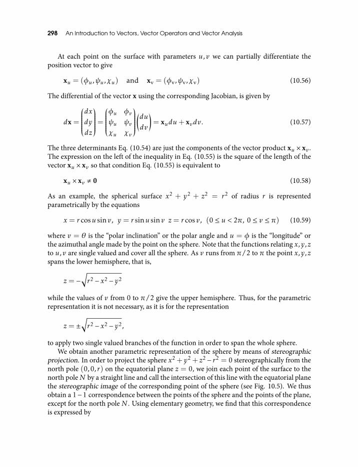
298 An Introduction to Vectors, Vector Operators and Vector Analysis
At each point on the surface with parameters u,v we can partially differentiate theposition vector to give
xu = (φu ,ψu ,χu) and xv = (φv,ψv,χv) (10.56)
The differential of the vector x using the corresponding Jacobian, is given by
dx =
dx
dy
dz
=φu φvψu ψvχu χv
(du
dv
)= xudu+ xvdv. (10.57)
The three determinants Eq. (10.54) are just the components of the vector product xu × xv .The expression on the left of the inequality in Eq. (10.55) is the square of the length of thevector xu × xv so that condition Eq. (10.55) is equivalent to
xu × xv , 0 (10.58)
As an example, the spherical surface x2 + y2 + z2 = r2 of radius r is representedparametrically by the equations
x = r cosu sinv, y = r sinu sinv z = r cosv, (0 ≤ u < 2π, 0 ≤ v ≤ π) (10.59)
where v = θ is the “polar inclination” or the polar angle and u = φ is the “longitude” orthe azimuthal angle made by the point on the sphere. Note that the functions relating x,y,zto u,v are single valued and cover all the sphere. As v runs from π/2 to π the point x,y,zspans the lower hemisphere, that is,
z = −√r2 − x2 − y2
while the values of v from 0 to π/2 give the upper hemisphere. Thus, for the parametricrepresentation it is not necessary, as it is for the representation
z = ±√r2 − x2 − y2,
to apply two single valued branches of the function in order to span the whole sphere.We obtain another parametric representation of the sphere by means of stereographic
projection. In order to project the sphere x2 + y2 + z2 − r2 = 0 stereographically from thenorth pole (0,0,r) on the equatorial plane z = 0, we join each point of the surface to thenorth poleN by a straight line and call the intersection of this line with the equatorial planethe stereographic image of the corresponding point of the sphere (see Fig. 10.5). We thusobtain a 1−1 correspondence between the points of the sphere and the points of the plane,except for the north pole N . Using elementary geometry, we find that this correspondenceis expressed by
Functions with Vector Arguments 299
x =2r2u
u2 + v2 + r2 , y =2r2v
u2 + v2 + r2 , z =(u2 + v2 − r2)r
u2 + v2 + r2 , (10.60)
Fig. 10.5 Stereographic projection of the sphere
where (u,v) are the rectangular (cartesian) coordinates of the image point in the plane.These equations can be regarded as the parametric representation of the sphere, theparameters (u,v) being the rectangular coordinates in the u,v (equatorial) plane.
As a further example, we give parametric representation of surfaces
x2
a2 +y2
b2 −z2
c2 = 1 andx2
a2 +y2
b2 −z2
c2 = −1
called the hyperboloid of one sheet and the hyperboloid of two sheets respectively(see Fig. 10.6). The hyperboloid of one sheet is represented by
x = acosu coshv,
y = b sinu coshv,
z = c sinhv (10.61)
where 0 ≤ u < 2π; −∞ < v <+∞ and the hyperboloid of two sheets by
x = acosu sinhv,
y = b sinu sinhv,
z = ±ccoshv (10.62)
where 0 ≤ u < 2π; 0 < v <+∞.In general, we may regard the parametric representation of a surface as the mapping of
the regionR of the (u,v) plane onto the corresponding surface. To each point of the region
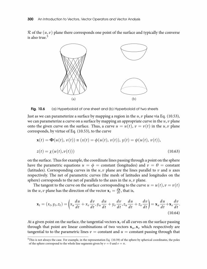
300 An Introduction to Vectors, Vector Operators and Vector Analysis
R of the (u,v) plane there corresponds one point of the surface and typically the converseis also true.5
Fig. 10.6 (a) Hyperboloid of one sheet and (b) Hyperboloid of two sheets
Just as we can parameterize a surface by mapping a region in the u,v plane via Eq. (10.53),we can parameterize a curve on a surface by mapping an appropriate curve in the u,v planeonto the given curve on the surface. Thus, a curve u = u(t), v = v(t) in the u,v planecorresponds, by virtue of Eq. (10.53), to the curve
x(t) =Φ(u(t), v(t)) ≡ (x(t) = φ(u(t), v(t)), y(t) = ψ(u(t), v(t)),
z(t) = χ(u(t),v(t))) (10.63)
on the surface. Thus for example, the coordinate lines passing through a point on the spherehave the parametric equations u = φ = constant (longitudes) and v = θ = constant(latitudes). Corresponding curves in the u,v plane are the lines parallel to v and u axesrespectively. The net of parametric curves (the mesh of latitudes and longitudes on thesphere) corresponds to the net of parallels to the axes in the u,v plane.
The tangent to the curve on the surface corresponding to the curve u = u(t),v = v(t)in the u,v plane has the direction of the vector xt = dx
dt , that is,
xt = (xt,yt,zt) =(xududt
+ xvdvdt
,yududt
+ yvdvdt
,zududt
+ zvdvdt
)= xu
dudt
+xvdvdt
.
(10.64)
At a given point on the surface, the tangential vectors xt of all curves on the surface passingthrough that point are linear combinations of two vectors xu ,xv which respectively aretangential to to the parametric lines v = constant and u = constant passing through that
5This is not always the case. For example, in the representation Eq. (10.59) of the sphere by spherical coordinates, the polesof the sphere correspond to the whole line segments given by v = 0 and v = π.
Functions with Vector Arguments 301
point. (e.g., the vectors φ and θ for the spherical polar coordinates on a sphere.) This meansthat the tangents all lie in the plane through the point spanned by the vectors xu and xv ,that is, the tangent plane to the surface at that point. The normal to the surface at thatpoint is perpendicular to all tangential directions, in particular to the vectors xu and xv .Thus, the surface normal is parallel (or antiparallel) to the direction of the vector product
xu × xv = (yuzv − yvzu ,zuxv − zvxu ,xuyv − xvyu). (10.65)
One of the most important keys to the understanding of the given surface is the study ofthe curves that lie on it. Here, we give the expression for the arc length s of such a curve.We start with(
dsdt
)2
=
(dxdt
)2
+
(dy
dt
)2
+
(dzdt
)2
= xt · xt,
so in view of Eq. (10.64) we get(dsdt
)2
=
(xududt
+ xvdvdt
)·(xududt
+ xvdvdt
)
=
(xududt
+ xvdvdt
)2
+
(yududt
+ yvdvdt
)2
+
(zududt
+ zvdvdt
)2
= E
(dudt
)2
+ 2F(dudt
)(dvdt
)+G
(dvdt
)2
. (10.66)
Here, the coefficients E,F,G, the Gaussian fundamental quantities of the surface, aregiven by
E =
(∂x∂u
)2
+
(∂y
∂u
)2
+
(∂z∂u
)2
= xu · xu
F =∂x∂u
∂x∂v
+∂y
∂u
∂y
∂v+∂z∂u
∂z∂v
= xu · xv
G =
(∂x∂v
)2
+
(∂y
∂v
)2
+
(∂z∂v
)2
= xv · xv (10.67)
These depend only on xu ,xv and therefore on the surface and its parametricrepresentation and not on the particular choice of the curve on the surface. The expressionEq. (10.66) for the derivative of the length of arc s with respect to the parameter t usually
302 An Introduction to Vectors, Vector Operators and Vector Analysis
is written symbolically without reference to the parameter used along the curve. One saysthat the line element ds is given by the quadratic differential form (“fundamental form”)
ds2 = Edu2 + 2Fdudv+Gdv2. (10.68)
The length of the cross product xu × xv can be expressed in terms of E,F,G as
|xu × xv |2 = |xu |2|xv |2 − (xu · xv)2 = EG −F2. (10.69)
Our original condition on the parametric representation (inequality Eq. (10.55)) can nowbe formulated as the condition
EG −F2 > 0 (10.70)
for the fundamental quantities.The direction cosines for one of the two normals to the surface are the components of
the unit vector
1|xu × xv |
xu × xv =1
√EG −F2
xu × xv .
It follows from Eq. (10.65) that the normal to a surface represented parametrically has thedirection cosines
cosα =yuzv − yvzu√EG −F2
, cosβ =zuxv − zvxu√EG −F2
, cosγ =xuyv − xvyu√EG −F2
. (10.71)
The tangent to a curve u = u(t),v = v(t) on the surface has the direction of the vector
xt = xududt
+ xvdvdt
.
If we now consider a second curve, u = u(τ),v = v(τ) on the surface referred to aparameter τ , its tangent has the direction of the vector
xτ = xududτ
+ xvdvdτ
.
If the two curves pass through the same point on the surface, the cosine of the angle ofintersection ω is the same as the cosine of the angle between xt and xτ . Hence,
cosω =xt · xτ|xt ||xτ |
.
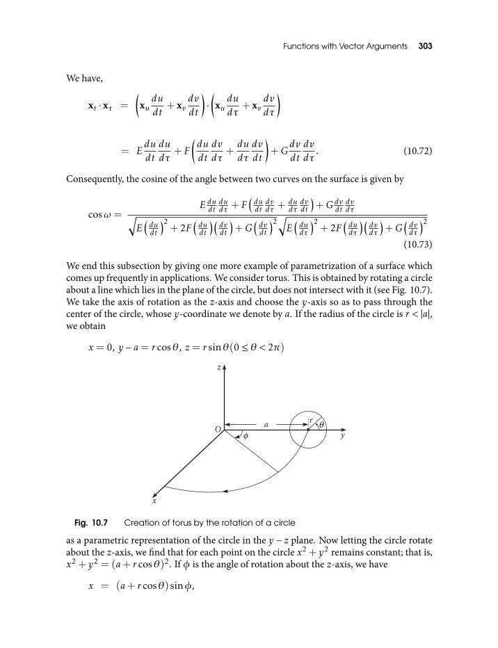
Functions with Vector Arguments 303
We have,
xt · xτ =
(xududt
+ xvdvdt
)·(xududτ
+ xvdvdτ
)
= Edudtdudτ
+ F
(dudtdvdτ
+dudτ
dvdt
)+G
dvdtdvdτ
. (10.72)
Consequently, the cosine of the angle between two curves on the surface is given by
cosω =E dudt
dudτ + F
(dudt
dvdτ +
dudτ
dvdt
)+G dv
dtdvdτ√
E(dudt
)2+ 2F
(dudt
)(dvdt
)+G
(dvdt
)2√E(dudτ
)2+ 2F
(dudτ
)(dvdτ
)+G
(dvdτ
)2
(10.73)
We end this subsection by giving one more example of parametrization of a surface whichcomes up frequently in applications. We consider torus. This is obtained by rotating a circleabout a line which lies in the plane of the circle, but does not intersect with it (see Fig. 10.7).We take the axis of rotation as the z-axis and choose the y-axis so as to pass through thecenter of the circle, whose y-coordinate we denote by a. If the radius of the circle is r < |a|,we obtain
x = 0, y − a= r cosθ, z = r sinθ(0 ≤ θ < 2π)
Fig. 10.7 Creation of torus by the rotation of a circle
as a parametric representation of the circle in the y − z plane. Now letting the circle rotateabout the z-axis, we find that for each point on the circle x2 + y2 remains constant; that is,x2 + y2 = (a+ r cosθ)2. If φ is the angle of rotation about the z-axis, we have
x = (a+ r cosθ)sinφ,
304 An Introduction to Vectors, Vector Operators and Vector Analysis
y = (a+ r cosθ)cosφ,
z = r sinθ (10.74)
with 0 ≤ φ < 2π,0 ≤ θ < 2π as a parametric representation of the torus in terms of theparameters θ and φ. In this representation the torus appears as the image of the square ofside 2π in the θ,φ plane. Any pair of boundary points of this square lying on the same lineθ = constant or φ = constant corresponds to only one point on the surface and the fourcorners of the square all correspond to the same point on the surface.
Equation (10.67) gives, for the line element on the torus,
ds2 = r2dθ2 + (a+ r cosθ)2dφ2.
10.13 The Divergence and the Curl of a Vector FieldWe have already seen that the del or the grad operator has vector like structure and it alsotransforms like a vector under the rotation and translation of the coordinate system. Thisenables us to formally treat the del operator like a vector with components
(∂∂x1
, ∂∂x2
, ∂∂x3
)and define its scalar and vector products with vector valued functions possibly giving avector field.
The divergenceThe corresponding scalar product called the divergence of a field is given by
∇ · f(x) =∂f1∂x1
+∂f2∂x2
+∂f3∂x3
=3∑k=1
∂fk∂xk
(10.75)
where f1,2,3(x) are the scalar valued component functions of the vector valued functionf(x) with respect to some orthonormal basis (see Eq. (10.1)). If we fix a position vectorx, then we get the corresponding vector f(x) giving us the unique value of the divergence∇·f(x). Thus, the divergence of a vector field is itself a scalar field and we can calculate ‘thedivergence at a point’. The value of the divergence of a vector field at a point is a measure ofhow much a vector f(x) spreads out from (or flows into) the point x in question. Thus, thevector function in Fig. 10.8(a) has large positive divergence (if the arrows pointed inwardit would be a large negative divergence), the function in Fig. 10.8(b) has zero divergenceand Fig. 10.8(c) again shows a function of positive divergence. Here is a nice possibleobservation of the divergence phenomenon [9]. Imagine standing at the edge of a pond.Sprinkle some sawdust on the surface. If the material spreads out then you have droppedit at a point of positive divergence; if it collects together, you have dropped it at a point ofnegative divergence. The vector function v in this model is the velocity of the water. Thisis a two dimensional example but it helps give us a feel for the meaning of divergence. Apoint of positive divergence is a sourse or ‘foucet’; a point of negative divergence is a sinkor ‘drain’.
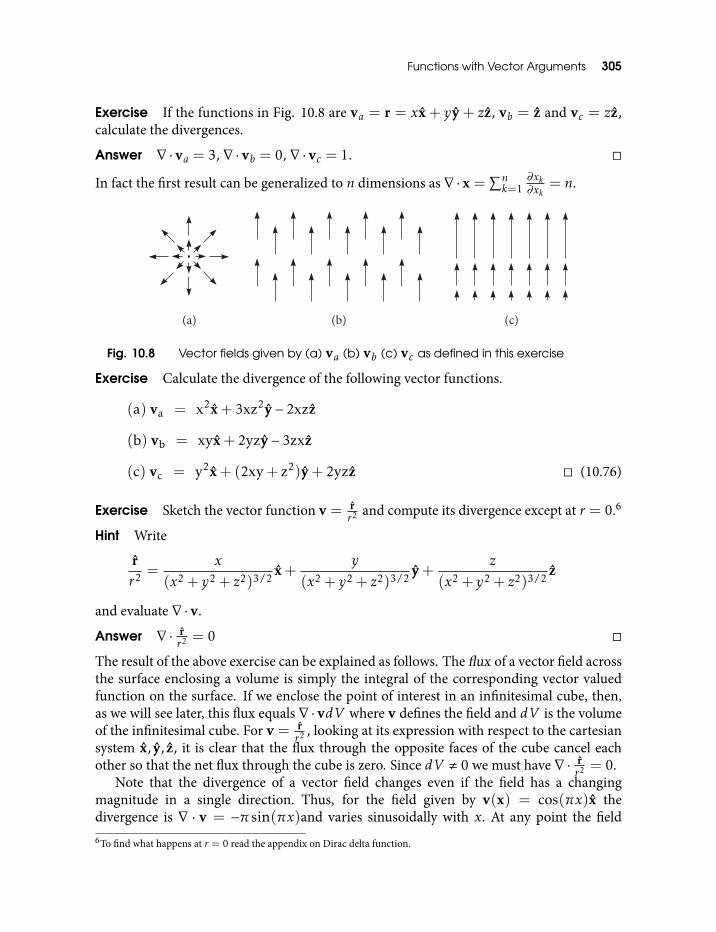
Functions with Vector Arguments 305
Exercise If the functions in Fig. 10.8 are va = r = xx + yy + zz, vb = z and vc = zz,calculate the divergences.
Answer ∇ · va = 3, ∇ · vb = 0, ∇ · vc = 1.
In fact the first result can be generalized to n dimensions as ∇ · x =∑nk=1
∂xk∂xk
= n.
Fig. 10.8 Vector fields given by (a) va (b) vb (c) vc as defined in this exercise
Exercise Calculate the divergence of the following vector functions.
(a) va = x2x+ 3xz2y− 2xzz
(b) vb = xyx+ 2yzy− 3zxz
(c) vc = y2x+ (2xy+ z2)y+ 2yzz (10.76)
Exercise Sketch the vector function v = rr2 and compute its divergence except at r = 0.6
Hint Write
rr2 =
x
(x2 + y2 + z2)3/2x+
y
(x2 + y2 + z2)3/2y+
z
(x2 + y2 + z2)3/2z
and evaluate ∇ · v.
Answer ∇ · rr2 = 0
The result of the above exercise can be explained as follows. The flux of a vector field acrossthe surface enclosing a volume is simply the integral of the corresponding vector valuedfunction on the surface. If we enclose the point of interest in an infinitesimal cube, then,as we will see later, this flux equals ∇ · vdV where v defines the field and dV is the volumeof the infinitesimal cube. For v = r
r2 , looking at its expression with respect to the cartesiansystem x, y, z, it is clear that the flux through the opposite faces of the cube cancel eachother so that the net flux through the cube is zero. Since dV , 0 we must have ∇ · r
r2 = 0.Note that the divergence of a vector field changes even if the field has a changing
magnitude in a single direction. Thus, for the field given by v(x) = cos(πx)x thedivergence is ∇ · v = −π sin(πx)and varies sinusoidally with x. At any point the field6To find what happens at r = 0 read the appendix on Dirac delta function.
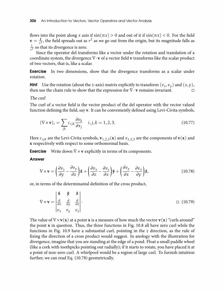
306 An Introduction to Vectors, Vector Operators and Vector Analysis
flows into the point along x axis if sin(πx) > 0 and out of it if sin(πx) < 0. For the fieldv = r
r2 , the field spreads out as r2 as we go out from the origin, but its magnitude falls as1r2 so that its divergence is zero.
Since the operator del transforms like a vector under the rotation and translation of acoordinate system, the divergence ∇·v of a vector field v transforms like the scalar productof two vectors, that is, like a scalar.
Exercise In two dimensions, show that the divergence transforms as a scalar underrotation.
Hint Use the rotation (about the z-axis) matrix explicitly to transform (vx,vy) and (x,y),then use the chain rule to show that the expression for ∇ · v remains invariant.
The curlThe curl of a vector field is the vector product of the del operator with the vector valuedfunction defining the field, say v. It can be conveniently defined using Levi-Civita symbols,
(∇× v)i =∑jk
εijk∂vk∂xj
i, j,k = 1,2,3. (10.77)
Here εijk are the Levi-Civita symbols, v1,2,3(x) and x1,2,3 are the components of v(x) andx respectively with respect to some orthonormal basis.
Exercise Write down ∇× v explicitly in terms of its components.
Answer
∇× v =
(∂vz∂y−∂vy∂z
)x+
(∂vx∂z− ∂vz∂x
)y+
(∂vy∂x− ∂vx∂y
)z, (10.78)
or, in terms of the determinantal definition of the cross product,
∇× v =
∣∣∣∣∣∣∣∣∣∣x y z∂∂x
∂∂y
∂∂z
vx vy vz
∣∣∣∣∣∣∣∣∣∣ · (10.79)
The value of ∇×v(x) at a point x is a measure of how much the vector v(x) “curls around”the point x in question. Thus, the three functions in Fig. 10.8 all have zero curl while thefunctions in Fig. 10.9 have a substantial curl, pointing in the z direction, as the rule offixing the direction of a cross product would suggest. In anology with the illustration fordivergence, imagine that you are standing at the edge of a pond. Float a small paddle wheel(like a cork with toothpicks pointing out radially); if it starts to rotate, you have placed it ata point of non-zero curl. A whirlpool would be a region of large curl. To furnish intuitionfurther, we can read Eq. (10.78) geometrically.
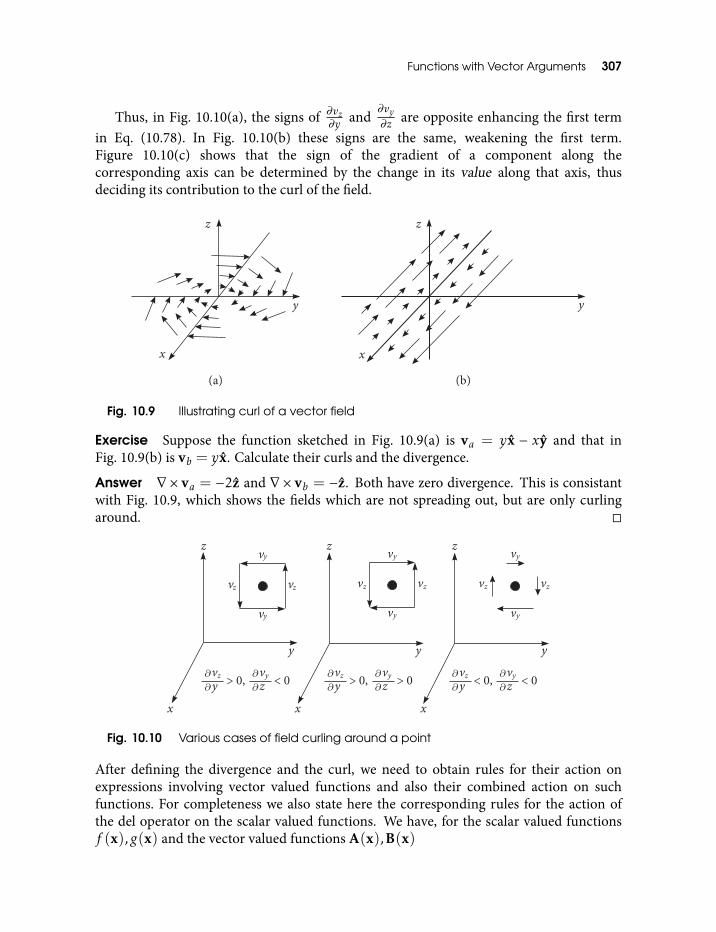
Functions with Vector Arguments 307
Thus, in Fig. 10.10(a), the signs of ∂vz∂y and
∂vy∂z are opposite enhancing the first term
in Eq. (10.78). In Fig. 10.10(b) these signs are the same, weakening the first term.Figure 10.10(c) shows that the sign of the gradient of a component along thecorresponding axis can be determined by the change in its value along that axis, thusdeciding its contribution to the curl of the field.
Fig. 10.9 Illustrating curl of a vector field
Exercise Suppose the function sketched in Fig. 10.9(a) is va = yx − xy and that inFig. 10.9(b) is vb = yx. Calculate their curls and the divergence.
Answer ∇× va = −2z and ∇× vb = −z. Both have zero divergence. This is consistantwith Fig. 10.9, which shows the fields which are not spreading out, but are only curlingaround.
Fig. 10.10 Various cases of field curling around a point
After defining the divergence and the curl, we need to obtain rules for their action onexpressions involving vector valued functions and also their combined action on suchfunctions. For completeness we also state here the corresponding rules for the action ofthe del operator on the scalar valued functions. We have, for the scalar valued functionsf (x),g(x) and the vector valued functions A(x),B(x)
308 An Introduction to Vectors, Vector Operators and Vector Analysis
∇(f + g) = ∇f +∇g, ∇ · (A+B) = ∇ ·A+∇ ·B
∇× (A+B) = ∇×A+∇×B,
and
∇(kf ) = k∇f ∇ · (kA) = k∇ ·A ∇× (kA) = k∇×A,
as can be easily checked using their definitions and the linearity of differentiation. Differentrules apply for different types of products of functions, that is, scalar valued products f gand A ·B and the vector valued products f A and A ×B. This leads to six product rules,two for gradients,
∇(f g) = f ∇g + g∇f , (10.80)
∇(A ·B) = A× (∇×B) +B× (∇×A) + (A · ∇)B+ (B · ∇)A, (10.81)
two for divergences,
∇ · (f A) = f (∇ ·A) +A · (∇f ), (10.82)
∇ · (A×B) = B · (∇×A)−A · (∇×B) (10.83)
and two for curls,
∇× (f A) = f (∇×A)−A× (∇f ), (10.84)
∇× (A×B) = (B · ∇)A− (A · ∇)B+A(∇ ·B)−B(∇ ·A). (10.85)
Exercise Prove Eq. (10.81).
Solution We successively take up all terms on the RHS. We have,
[A× (∇×B)]i =∑jklm
εkijεklmAj∂Bm∂xl
.
Using
εkijεklm = δilδjm − δimδjl
we get
[A× (∇×B)]i =∑j
Aj
(∂Bj∂xi− ∂Bi∂xj
).
Functions with Vector Arguments 309
Similarly,
[B× (∇×A)]i =∑j
Bj
(∂Aj∂xi− ∂Ai∂xj
).
Further, we get for the last two terms,
[(A · ∇)B]i =∑j
Aj∂Bi∂xj
and
[(B · ∇)A]i =∑j
Bj∂Ai∂xj
.
Putting all terms together, we get, for the ith component of the RHS,∑j
(Aj∂Bj∂xi
+Bj∂Aj∂xi
)= [∇(A ·B)]i .
Exercise Prove Eq. (10.83).
Solution
∇ · (A×B) =∂∂xi
(A×B)i =∂∂xi
(εijkAjBk)
= εijk∂Aj∂xi
Bk + εijk∂Bk∂xi
Aj
= (∇×A)kBk − (∇×B)jAj
= B · (∇×A)−A · (∇×B). (10.86)
Here are the rules for differentiating quotients,
∇(f
g
)=
g∇f − f ∇gg2
∇ ·(
Ag
)=
g(∇ ·A)−A · (∇g)g2
∇×(
Ag
)=
g(∇×A) +A× (∇g)g2 (10.87)
310 An Introduction to Vectors, Vector Operators and Vector Analysis
All the above rules for differentiating expressions of functions are valid for alldifferentiable functions, scalar or vector valued, as the case may be. Therefore, these rulescan be treated as vector identities involving differential operators. You may try and proveall these identities using Levi-Civita symbols.
Second derivativesUpto now we obtained rules to find different types of derivatives of expressions involvingvarious types of functions. We shall now find rules to evaluate second derivatives obtainedby combining different types of first derivatives, namely, the gradient, the divergence andthe curl. Since∇f is a vector for a scalar valued function f , we can take the divergence andthe curl of it. We have,
(i) Divergence of the gradient: ∇2f ≡ ∇ · (∇f ).
(ii) Curl of gradient: ∇× (∇f ).The divergence ∇ · v is a scalar, so we can take its gradient :
(iii) Gradient of divergence: ∇(∇ · v).The curl ∇× v is a vector, so we can take its divergence and curl :
(iv) Divergence of curl: ∇ · (∇× v).
(v) Curl of a curl: ∇× (∇× v).
These are all the possibilities and we consider them one by one.
(i) The operator ∇2f defined above is called the Laplacian of f . We have,
∇2f ≡ ∇ · (∇f ) =
(x∂∂x
+ y∂∂y
+ z∂∂z
)·(∂f
∂xx+
∂f
∂yy+
∂f
∂zz)
=∂2f
∂x2 +∂2f
∂y2 +∂2f
∂z2 . (10.88)
The Laplacian of a scalar valued function is a scalar.
Exercise Show that the Laplacian of a scalar field φ(x) at a point is proportional tothe difference between the value of φ at that point and the average value of φ at thesurrounding points.
Solution Let φ0 be the value of φ at a point which we take to be the origin. Letφ(±∆x), φ(±∆y) and φ(±∆z) be the values at points ±∆x,±∆y,±∆z respectively.We can approximate the second order partial derivatives defining the Laplacian bythe corresponding second order differences
∂2φ
∂x2 =φ(∆x) +φ(−∆x)− 2φ0
∆x2
Functions with Vector Arguments 311
∂2φ
∂y2 =φ(∆y) +φ(−∆y)− 2φ0
∆y2
∂2φ
∂z2 =φ(∆z) +φ(−∆z)− 2φ0
∆z2 .
Taking ∆x = ∆y = ∆z = ∆ and then adding these ratios we get
∇2φ =−6∆2
[φ0 −
16φ(∆x) +φ(−∆x) +φ(∆y) +φ(−∆y) +φ(∆z) +φ(−∆z)
]=−6∆2 (φ0 −φavg).
If the Laplacian at a point is negative then its value at that point exceeds average ofits values at the surrounding neighbours. Since φ is a continuous and differentiablefunction, its values cannot differ drastically at nearby points. Thus, if ∇2φ < 0 at apoint, this point represents a local maximum of φ. On the other hand, if ∇2φ > 0at a point this point must be a local minimum of φ. Since negative divergence at apoint corresponds to the inflow of the field into that point, ∇2φ < 0 corresponds tothe inflow of the field ∇φ towards the point of maximum φ. ∇2φ > 0 correspondsto a point of local minimum of φ and the field ∇φ diverges out of this point. Youcan draw the maximum and a minimum (a peak and a valley) for a function of twovariables and draw ∇φ vectors perpendicular to the contours of constant φ values.Then you can varify the above statements with reference to these pictures.
Exercise Explicitly calculate ∇2φ for φ = 1r , r , 0 and show that it vanishes.
We may occasionally encounter the Laplcian of a vector, ∇2v which is a vectorquantity whose x-component is the Laplacian of vx etc,7. We have,
∇2v ≡ (∇2vx)x+ (∇2vy)y+ (∇2vz)z. (10.89)
(ii) The curl of a gradient is always zero. That is,
∇× (∇f ) = 0. (10.90)
Exercise Prove Eq. (10.90).
Solution We have,
[∇× (∇f )]i = εijk∂2f
∂xj∂xk.
7For curvilinear coordinates, where the unit vectors themselves depend on position, they too must be differentiated.
312 An Introduction to Vectors, Vector Operators and Vector Analysis
In this double sum, the pairs of terms like ∂2f∂x1∂x2
and ∂2f∂x2∂x1
occur with oppositesigns and cancel8 and all terms can be paired this way. Hence, the sum vanishes andwe get
[∇× (∇f )]i = 0, i = 1,2,3.
(iii) ∇(∇ · v) seldom occurs in physical applications. Note that ∇2v , ∇(∇ · v).(iv) The divergence of a curl, like the curl of a gradient, is always zero.
∇ · (∇× v) = 0. (10.91)
Exercise Prove Eq. (10.91).
Solution
∇ · (∇× v) = εijk∂2vk∂xi∂xj
.
In this triple sum, for a fixed value of k, two terms occur with interchanged values ofindices i and j . These terms are identical but with opposite signs and hence cancel.All terms occur in such pairs so that the sum vanishes, thus proving Eq. (10.91).
(v) The curl of curl operator can be decomposed into the gradient of divergence and thevector Laplacian as follows.
∇× (∇× v) = ∇(∇ · v)−∇2v. (10.92)
Exercise Prove Eq. (10.92).
Solution
[∇× (∇× v)]i = εkijεklm∂2vm∂xj∂xl
Using
εkijεklm = δilδjm − δimδjl
this becomes
∂∂xi
(∂vj∂xj
)− ∂
2vi∂x2
j
= [∇(∇ · v)]i − [∇2v]i .
Note that Eq. (10.92) can be taken to be a coordinate free definition of ∇2v in preferenceto Eq. (10.89) which depends on cartesian coordinates.
8We assume, of course, that the order of differentiation does not matter.
Functions with Vector Arguments 313
Exercise In what follows r denotes a position vector r = |r| is its magnitude, A(r) andB(r) are vector fields, φ(r) is a scalar field and f (r) is a function of r . All fields andfunctions have continuous first derivatives. Using Levi-Civita symbols or otherwise, provethe following.
(i) ∇× (∇×A) = ∇(∇ ·A)−∇2A.(ii) A× (∇×B) = ∇B(A ·B)− (A · ∇)B where ∇B operates on B only.
(iii) Given ∇×A = 0 = ∇×B show that ∇ · (A×B) = 0.(iv) For constant a and b show that ∇× [(a× r)×b] = a×b.(v) ∇ · r = 3, ∇× r = 0, ∇(A · r) = A, (A · ∇)r = A.
(vi) ∇rn = nrn−2r, ∇ · f (r)rr = 1r2
ddr (r
2f ).
We will use any one or more of these results in the sequel, as and when required.
Exercise A particle performs uniform circular motion on a circle of radius r and positionvector r. Show that (a) ∇× v = 2ω and (b) ∇ · v = 0, where v is the linear velocity and ωis the (constant) rotational velocity of the particle.
Solution
(a) We know that for circular motion, v = ω × r. Therefore,
∇× v = ∇× (ω × r) = ω(∇ · r)−ω · ∇r.
However,∇·r = 3 andω ·∇r = ω, which gives (a). Thus, we see that the curl operatortransforms the velocity vector into a rotational velocity vector.
(b) ∇ · v = ∇ · (ω × r) = r · ∇ × ω − ω · ∇ × r = 0, since ω is a constant vector and∇× r = 0.
Thus, there are basically two types of second derivatives, the Laplacian, which is offundamental importance and the gradient of divergence which we seldom encounter.Since the second derivatives suffice to deal with practically all the physical applications,going over to higher derivatives will reduce to an academic exercise without any physicalmotivation.
10.14 Differential Operators in Curvilinear CoordinatesA system of curvilinear coordinates, say (u,v,w), is specified via an invertible passivetransformation R3 7→R3:
(x,y,z) 7→ (u(x,y,z),v(x,y,z),w(x,y,z)) (10.93)
or via the inverse R3 7→R3 transformation
(u,v,w) 7→ (x(u,v,w),y(u,v,w),z(u,v,w)). (10.94)
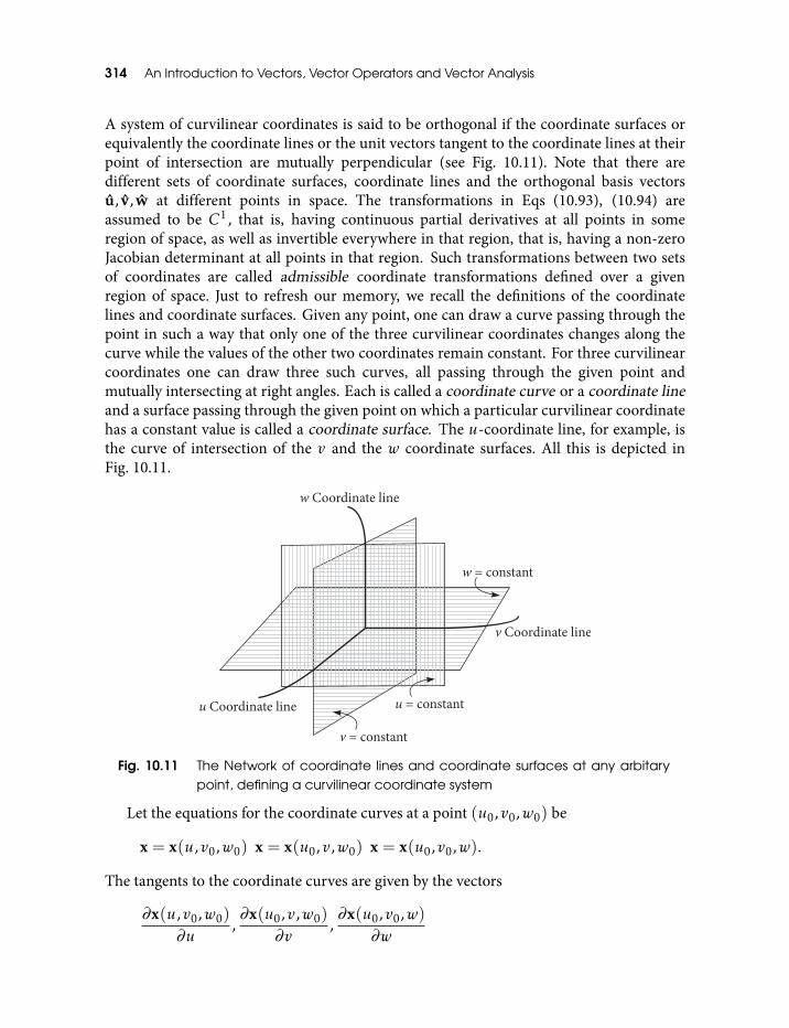
314 An Introduction to Vectors, Vector Operators and Vector Analysis
A system of curvilinear coordinates is said to be orthogonal if the coordinate surfaces orequivalently the coordinate lines or the unit vectors tangent to the coordinate lines at theirpoint of intersection are mutually perpendicular (see Fig. 10.11). Note that there aredifferent sets of coordinate surfaces, coordinate lines and the orthogonal basis vectorsu, v,w at different points in space. The transformations in Eqs (10.93), (10.94) areassumed to be C1, that is, having continuous partial derivatives at all points in someregion of space, as well as invertible everywhere in that region, that is, having a non-zeroJacobian determinant at all points in that region. Such transformations between two setsof coordinates are called admissible coordinate transformations defined over a givenregion of space. Just to refresh our memory, we recall the definitions of the coordinatelines and coordinate surfaces. Given any point, one can draw a curve passing through thepoint in such a way that only one of the three curvilinear coordinates changes along thecurve while the values of the other two coordinates remain constant. For three curvilinearcoordinates one can draw three such curves, all passing through the given point andmutually intersecting at right angles. Each is called a coordinate curve or a coordinate lineand a surface passing through the given point on which a particular curvilinear coordinatehas a constant value is called a coordinate surface. The u-coordinate line, for example, isthe curve of intersection of the v and the w coordinate surfaces. All this is depicted inFig. 10.11.
Fig. 10.11 The Network of coordinate lines and coordinate surfaces at any arbitarypoint, defining a curvilinear coordinate system
Let the equations for the coordinate curves at a point (u0,v0,w0) be
x = x(u,v0,w0) x = x(u0,v,w0) x = x(u0,v0,w).
The tangents to the coordinate curves are given by the vectors
∂x(u,v0,w0)
∂u,∂x(u0,v,w0)
∂v,∂x(u0,v0,w)
∂w
Functions with Vector Arguments 315
respectively. Orthogonality of these vectors requires that
∂x∂u· ∂x∂v
=∂x∂u· ∂x∂w
=∂x∂v· ∂x∂w
= 0.
We are interested in the differential displacement dx as we go from x(u,v,w) to x(u +du,v+ dv,w+ dw). We have, in terms of the corresponding Jacobian matrix,
dx =
∂s1∂u
∂s1∂v
∂s1∂w
∂s2∂u
∂s2∂v
∂s2∂w
∂s3∂u
∂s3∂v
∂s3∂w
dudvdw
= ∂x∂udu+
∂x∂udv+
∂x∂w
dw = xudu+ xvdv+ xwdw.
(10.95)
where s1,2,3(u,v,w) = x(u,v,w)·u, v,w are the components of x in the u, v,w mutuallyorthogonal directions. This defines the line element ds = |dx| via
ds2 = dx · dx = xu · xudu2 + xv · xvdv2 + xw · xwdw2
= h21du
2 + h22dv
2 + h23dw
2. (10.96)
The parameters h1,h2,h3 are the analogues of the Gaussian fundamental quantities E,F,Gof a surface, we derived before. They relate the differential displacements along the u, v,wdirections as a result of the displacement dx to the diferentials du,dv,dw via
dx = ds1u+ ds2v+ ds3w = h1duu+ h2dvv+ h3dww.
Thus, the volume of the rectangular parallelepiped with sides ds1,ds2,ds3 is given by
dV = ds1ds2ds3 = h1h2h3dudvdw.
The product h1h2h3 ensures that the the last term has the dimension of volume; as thecurvilinear coordinates can be dimensionless quantities like angles.
The u coordinate surface passing through the point (u0,v0,w0) is the collection ofpoints (x,y,z) satisfying u(x,y,z) = u0 and similarly, the v and w coordinate surfacesare given by v(x,y,z) = v0 and w(x,y,z) = w0, where (x,y,z) are the Cartesiancoordinates with respect to some rectangular Cartesian coordinate system. We can varythe point (u0,v0,w0) over the region for which the curvilinear coordinatetransformations, Eqs (10.93), (10.94), are defined. Therefore, we can replace u0,v0,w0 inthe equations defining the coordinate surfaces by u,v,w and say that a particular triad ofcoordinate surfaces emerges when particular values of u, v and w are substituted on theRHS of these equations. Thus, we write, for the equations defining the coordinate surfaces
u = u(x,y,z) v = v(x,y,z) w = w(x,y,z).
316 An Introduction to Vectors, Vector Operators and Vector Analysis
The normals to the coordinate surfaces are given by ∇u,∇v,∇w (see section 10.8) which,owing to orthogonality, must satisfy
0 = ∇u · ∇v = ∇u · ∇w = ∇v · ∇w.
The vectors normal to the coordinate surfaces are tangent to the corresponding coordinatecurves so that we can define the fundamental triad for the curvilinear coordinates as
u =∇u|∇u|
v =∇v|∇v|
w =∇w|∇w|
. (10.97)
Let ds1 = ds1u, ds2 = ds2v, ds3 = ds3w be the differential displacement along theu, v,w directions. Since ∇u,∇v,∇w have the same values in all the orthonormal basistriads and since ∇u,ds1, ∇v,ds2 and ∇w,ds3 are the pairs of parallel vectors, we canwrite,
du = ∇u · ds1 = |∇u||ds1|,
dv = ∇v · ds2 = |∇v||ds2|,
dw = ∇w · ds3 = |∇w||ds3|. (10.98)
This gives,
ds2 = ds21 + ds22 + ds
23 =
du2
|∇u|2+dv2
|∇v|2+dw2
|∇w|2. (10.99)
Comparing equations Eqs (10.96) and (10.99) we get
h1 =1|∇u|
=√
xu · xu impling u = h1∇u,
h2 =1|∇v|
=√
xv · xv impling v = h2∇v,
h3 =1|∇w|
=√
xw · xw impling w = h3∇w. (10.100)
Example For spherical polar coordinates we identify u = r, v = θ and w = φ, where
r =√x2 + y2 + z2, θ = cos−1
z√x2 + y2 + z2
and φ = tan−1(y
x
).
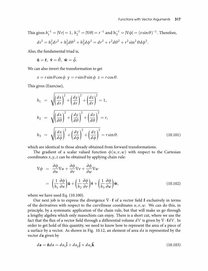
Functions with Vector Arguments 317
This gives h−11 = |∇r |= 1, h−1
2 = |∇θ|= r−1 and h−13 = |∇φ|= (rsinθ)−1. Therefore,
ds2 = h21dr
2 + h22dθ
2 + h23dφ
2 = dr2 + r2dθ2 + r2 sin2θdφ2.
Also, the fundamental triad is,
u = r, v = θ, w = φ.
We can also invert the transformation to get
x = r sinθ cosφ y = r sinθ sinφ z = r cosθ.
This gives (Exercise),
h1 =
√(dxdr
)2
+
(dy
dr
)2
+
(dzdr
)2
= 1,
h2 =
√(dxdθ
)2
+
(dy
dθ
)2
+
(dzdθ
)2
= r,
h3 =
√(dxdφ
)2
+
(dy
dφ
)2
+
(dzdφ
)2
= r sinθ. (10.101)
which are identical to those already obtained from forward transformations.The gradient of a scalar valued function φ(u,v,w) with respect to the Cartesian
coordinates x,y,z can be obtained by applying chain rule:
∇φ =∂φ
∂u∇u+
∂φ
∂v∇v+
∂φ
∂w∇w
=
(1h1
∂φ
∂u
)u+
(1h2
∂φ
∂v
)v+
(1h3
∂φ
∂w
)w, (10.102)
where we have used Eq. (10.100).Our next job is to express the divergence ∇ · f of a vector field f exclusively in terms
of the derivatives with respect to the curvilinear coordinates u,v,w. We can do this, inprinciple, by a systematic application of the chain rule, but that will make us go througha lengthy algebra which only masochists can enjoy. There is a short cut, where we use thefact that the flux of a vector field through a differential volume dV is given by ∇ · fdV . Inorder to get hold of this quantity, we need to know how to represent the area of a piece ofa surface by a vector. As shown in Fig. 10.12, an element of area da is represented by thevector da given by
da = nda= dax i+ day j+ dazk (10.103)
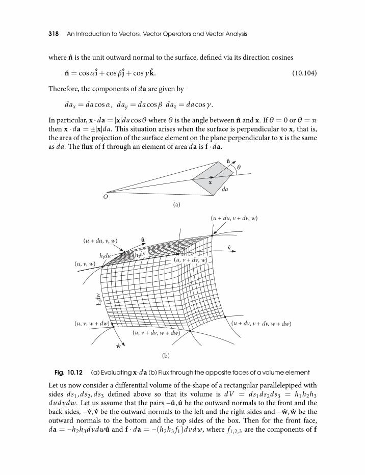
318 An Introduction to Vectors, Vector Operators and Vector Analysis
where n is the unit outward normal to the surface, defined via its direction cosines
n = cosαi+ cosβj+ cosγk. (10.104)
Therefore, the components of da are given by
dax = dacosα, day = dacosβ daz = dacosγ .
In particular, x ·da = |x|dacosθ where θ is the angle between n and x. If θ = 0 or θ = πthen x · da = ±|x|da. This situation arises when the surface is perpendicular to x, that is,the area of the projection of the surface element on the plane perpendicular to x is the sameas da. The flux of f through an element of area da is f · da.
Fig. 10.12 (a) Evaluating x·da (b) Flux through the opposite faces of a volume element
Let us now consider a differential volume of the shape of a rectangular parallelepiped withsides ds1,ds2,ds3 defined above so that its volume is dV = ds1ds2ds3 = h1h2h3dudvdw. Let us assume that the pairs −u, u be the outward normals to the front and theback sides, −v, v be the outward normals to the left and the right sides and −w,w be theoutward normals to the bottom and the top sides of the box. Then for the front face,da = −h2h3dvdwu and f · da = −(h2h3f1)dvdw, where f1,2,3 are the components of f
Functions with Vector Arguments 319
along u, v,w respectively and the product h2h3f1 is to be evaluated at u. On the back face,product h2h3f1 is to be evaluated at u + du so that f · da = (h2h3f1 + ∂
∂u (h2h3f1)du)dvdw. Therefore, the net flux through the front and back pair of faces is[
∂∂u
(h2h3f1)
]dudvdw =
1h1h2h3
∂∂u
(h2h3f1)dV .
In the same way, the right and the left sides give
1h1h2h3
∂∂v
(h1h3f2)dV
and the bottom and the top sides contribute
1h1h2h3
∂∂w
(h1h2f3)dV .
Thus, the total flux through the box is given by
(∇ · f)dV =1
h1h2h3
[∂∂u
(h2h3f1) +∂∂v
(h1h3f2) +∂∂w
(h1h2f3)
]dV
This gives
∇ · f = 1h1h2h3
[∂∂u
(h2h3f1) +∂∂v
(h3h1f2) +∂∂w
(h1h2f3)
]. (10.105)
Combining Eq. (10.105) with Eq. (10.102) we get, for the Laplacian operator,
∇2φ = ∇ ·∇φ =1
h1h2h3
[∂∂u
(h2h3
h1
∂φ
∂u
)+∂∂v
(h3h1
h2
∂φ
∂v
)+
∂∂w
(h1h2
h3
∂φ
∂w
)].
(10.106)
Our last task in this subsection is to express the curl ∇× f of a vector field f in terms of thederivatives with respect to the curvilinear coordinates u,v,w. The principle we follow forthis is
Circulation of f around a loop enclosing an infinitesimal area da = (∇×f)·da.
The sense of circulation is given by that which makes a right handed screw advance in thedirection of da. The required circulation can be explicitly calculated for an infinitesimalloop of rectangular shape. For each side of the rectangle, we have to find the scalarproduct of f with the vector along the side and in the direction consistent with the sense ofcirculation. In the first place, the surface enclosed by an infinitesimal loop can be taken tobe a plane. Consider such a rectangular loop in the u, v plane, with w normal to it

320 An Introduction to Vectors, Vector Operators and Vector Analysis
(see Fig. 10.13). From Fig. 10.13 and w pointing out of the page, it is clear that the sense ofcirculation which makes a right handed screw advance in w direction is counterclockwise,as shown. The vector on the side along u is ds1 = h1duu that on the side along v isds2 = h2dvv and area
da = h1h2dudvw.
Fig. 10.13 Circulation around a loop
Along the bottom side (along u) the contribution of f to circulation is
f · ds1 = h1f1du
Along the top side, the sign is reversed and h1f1 is evaluated at v+ dv rather than v. Bothsides together give[
−(h1f1)∣∣∣∣v+dv
+ (h1f1)∣∣∣∣v
]du = −
[∂∂v
(h1f1)
]dudv.
Similarly, the right and the left sides yield[∂∂u
(h2f2)
]dudv.
So, the total circulation is[∂∂u
(h2f2)−∂∂v
(h1f1)
]dudv =
1h1h2
[∂∂u
(h2f2)−∂∂v
(h1f1)
]w · da.
The coefficient of da serves to define thew component of the curl. Constructing the u andv components in the same way, we get
Functions with Vector Arguments 321
∇× f =1
h2h3
[∂∂v
(h3f3)−∂∂w
(h2f2)
]u+
1h1h3
[∂∂w
(h1f1)−∂∂u
(h3f3)
]v
+1
h1h2
[∂∂u
(h2f2)−∂∂v
(h1f1)
]w. (10.107)
This expression for ∇× f can be written in a compact determinantal form as
∇× f =1
h1h2h3
∣∣∣∣∣∣∣∣∣∣h1u h2v h3w∂∂u
∂∂v
∂∂w
h1f1 h2f2 h3f3
∣∣∣∣∣∣∣∣∣∣ · (10.108)
Exercise Express the vector derivatives, that is, gradient, divergence, curl and Laplacianin terms of (a) spherical polar and (b) cylindrical coordinates for a scalar field u(x) and avector field v(x).
Answer
(a) Gradient:
∇u =∂u∂r
r+1r∂u∂θθ+
1r sinθ
∂u∂φ
φ.
Divergence:
∇ · v =1r2∂∂r
(r2vr) +1
r sinθ∂∂θ
(sinθvθ) +1
r sinθ
∂vφ∂φ
.
Curl:
∇× v =1
r sinθ
[∂∂θ
(sinθvφ)−∂vθ∂φ
]r+
1r
[1
sinθ∂vr∂φ− ∂∂r
(rvφ)
]
θ+1r
[∂∂r
(rvθ)−∂vr∂θ
]φ.
Laplacian:
∇2u =1r2∂∂r
(r2∂u∂r
)+
1r2 sinθ
∂∂θ
(sinθ
∂u∂θ
)+
1
r2 sin2θ
∂2u
∂φ2 .
(b) Gradient:
∇u =∂u∂ρρ+
1ρ∂u∂φ
φ+∂u∂z
z.
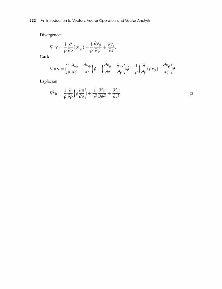
322 An Introduction to Vectors, Vector Operators and Vector Analysis
Divergence:
∇ · v =1ρ∂∂ρ
(ρvρ) +1ρ
∂vφ∂φ
+∂vz∂z
.
Curl:
∇× v =
(1ρ∂vz∂φ−∂vφ∂z
)ρ+
(∂vρ∂z− ∂vz∂ρ
)φ+
1ρ
(∂∂ρ
(ρvφ)−∂vρ∂φ
)z.
Laplacian:
∇2u =1ρ∂∂ρ
(ρ∂u∂ρ
)+
1ρ2∂2u
∂φ2 +∂2u
∂z2 .
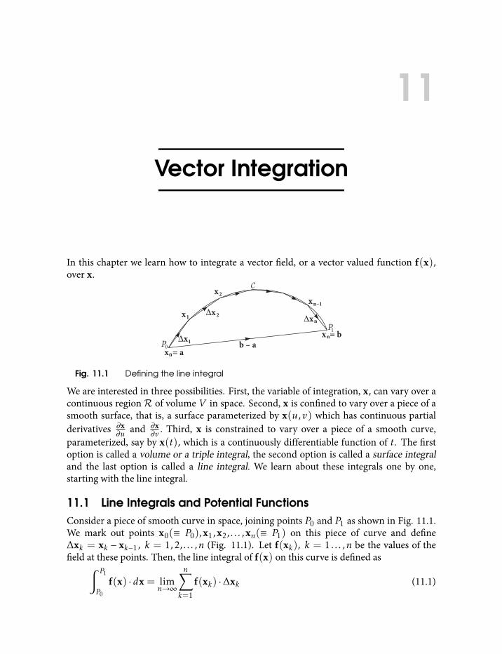
11
Vector Integration
In this chapter we learn how to integrate a vector field, or a vector valued function f(x),over x.
Fig. 11.1 Defining the line integral
We are interested in three possibilities. First, the variable of integration, x, can vary over acontinuous regionR of volume V in space. Second, x is confined to vary over a piece of asmooth surface, that is, a surface parameterized by x(u,v) which has continuous partialderivatives ∂x
∂u and ∂x∂v . Third, x is constrained to vary over a piece of a smooth curve,
parameterized, say by x(t), which is a continuously differentiable function of t. The firstoption is called a volume or a triple integral, the second option is called a surface integraland the last option is called a line integral. We learn about these integrals one by one,starting with the line integral.
11.1 Line Integrals and Potential FunctionsConsider a piece of smooth curve in space, joining points P0 and P1 as shown in Fig. 11.1.We mark out points x0(≡ P0),x1,x2, . . . ,xn(≡ P1) on this piece of curve and define∆xk = xk − xk−1, k = 1,2, . . . ,n (Fig. 11.1). Let f(xk), k = 1 . . . ,n be the values of thefield at these points. Then, the line integral of f(x) on this curve is defined as∫ P1
P0
f(x) · dx = limn→∞
n∑k=1
f(xk) ·∆xk (11.1)
324 An Introduction to Vectors, Vector Operators and Vector Analysis
In the limit as n→∞ the vectors ∆xk become tangent to the curve, so we are projecting thefield values f(xk) along the tangent at that point to the curve summing the correspondingproducts along the curve. Thus, the value of the line integral is influenced by both the fieldas well as the curve along which the integral is taken. Later, we will obtain conditions underwhich the value of a line integral depends only on the field values at the end points and noton the curve joining them.
The line integral in Eq. (11.1) can be transformed using the fact that the curve isparameterized by a continuously differentiable function x(t). Let x0 = x(T1) andxn = x(T2) correspond to the end points P0 and P1 respectively. We choose valuest0 = T1, t1, t2, . . . , tn = T2 in the closed interval [T1,T2] and let xk = x(tk). We define∆xk = ∆x(tk) = x(tk) − x(tk−1) and ∆tk = tk − tk−1. Then the line integral in Eq. (11.1)gets transformed to∫ T2
T1
f(x(t)) · x(t)dt = limn→∞
n∑k=1
f(x(tk)) ·(∆x(tk)∆tk
)∆tk (11.2)
where x(t) = dx(t)dt is the velocity or the tangent vector to the curve at the point x(t). If we
resolve the field along some fixed orthonormal basis then the line integral becomes
3∑i=1
∫ T2
T1
fi(x1(t),x2(t),x3(t))xi(t)dt (11.3)
where f1,2,3 and x1,2,3 are the components of f(x) and x respectively with respect to thefixed orthonormal basis. In particular, for a scalar valued function f (x) the line integralbecomes∫ T2
T1
f (x1(t),x2(t),x3(t))dt (11.4)
where x(t) ≡ (x2(t),x2(t),x3(t)) is the parametric description of the curve.
Exercise Let the position vectors of the points P0 and P1 be a and b respectively. Find∫ P1
P0dx.
Solution Notice that no curve joining P0 and P1 is specified. In fact it is not necessary.Whichever way we choose a curve joining P0 and P1 and construct the set ∆xi, all thevectors ∆xi add up to the vector b− a (see Fig. 11.1). The integral is∫ P1
P0
dx = b− a,
whose value depends only on the end points and not on the path connecting them.
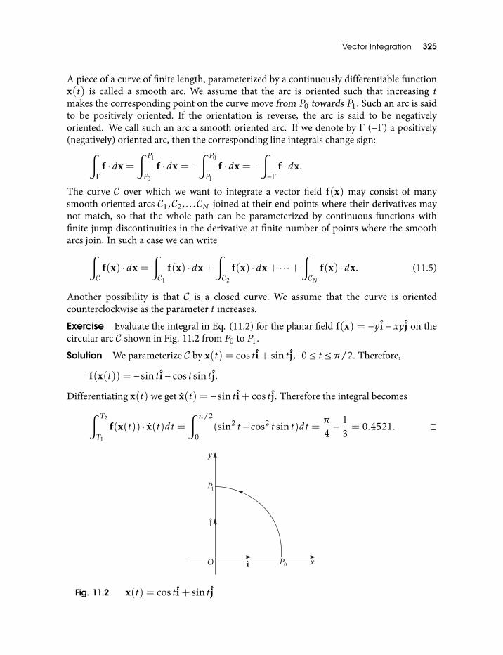
Vector Integration 325
A piece of a curve of finite length, parameterized by a continuously differentiable functionx(t) is called a smooth arc. We assume that the arc is oriented such that increasing tmakes the corresponding point on the curve move from P0 towards P1. Such an arc is saidto be positively oriented. If the orientation is reverse, the arc is said to be negativelyoriented. We call such an arc a smooth oriented arc. If we denote by Γ (−Γ ) a positively(negatively) oriented arc, then the corresponding line integrals change sign:∫
Γ
f · dx =
∫ P1
P0
f · dx = −∫ P0
P1
f · dx = −∫−Γ
f · dx.
The curve C over which we want to integrate a vector field f(x) may consist of manysmooth oriented arcs C1,C2, . . .CN joined at their end points where their derivatives maynot match, so that the whole path can be parameterized by continuous functions withfinite jump discontinuities in the derivative at finite number of points where the smootharcs join. In such a case we can write∫
Cf(x) · dx =
∫C1
f(x) · dx+∫C2
f(x) · dx+ · · ·+∫CN
f(x) · dx. (11.5)
Another possibility is that C is a closed curve. We assume that the curve is orientedcounterclockwise as the parameter t increases.
Exercise Evaluate the integral in Eq. (11.2) for the planar field f(x) = −y i− xy j on thecircular arc C shown in Fig. 11.2 from P0 to P1.
Solution We parameterize C by x(t) = cos ti+ sin tj, 0 ≤ t ≤ π/2. Therefore,
f(x(t)) = −sin ti− cos t sin tj.
Differentiating x(t) we get x(t) = −sin ti+ cos tj. Therefore the integral becomes∫ T2
T1
f(x(t)) · x(t)dt =∫ π/2
0(sin2 t − cos2 t sin t)dt =
π4− 1
3= 0.4521.
Fig. 11.2 x(t) = cos ti+ sin tj
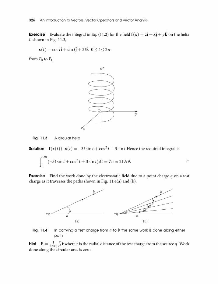
326 An Introduction to Vectors, Vector Operators and Vector Analysis
Exercise Evaluate the integral in Eq. (11.2) for the field f(x) = zi+ xj+ yk on the helixC shown in Fig. 11.3,
x(t) = cos ti+ sin tj+ 3tk 0 ≤ t ≤ 2π
from P0 to P1.
Fig. 11.3 A circular helix
Solution f(x(t)) · x(t) = −3t sin t+ cos2 t+ 3sin t Hence the required integral is∫ 2π
0(−3t sin t+ cos2 t+ 3sin t)dt = 7π ≈ 21.99.
Exercise Find the work done by the electrostatic field due to a point charge q on a testcharge as it traverses the paths shown in Fig. 11.4(a) and (b).
Fig. 11.4 In carrying a test charge from a to b the same work is done along eitherpath
Hint E = 14πε0
qr2 r where r is the radial distance of the test charge from the source q. Work
done along the circular arcs is zero.
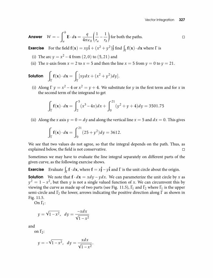
Vector Integration 327
Answer W = −∫ b
aE · ds =
q
4πε0
(1ra− 1rb
)for both the paths.
Exercise For the field f(x) = xy i+ (x2 + y2)j find∫Γ
f(x) · dx where Γ is
(i) The arc y = x2 − 4 from (2,0) to (5,21) and(ii) The x-axis from x = 2 to x = 5 and then the line x = 5 from y = 0 to y = 21.
Solution∫Γ
f(x) · dx =
∫Γ
[xydx+ (x2 + y2)dy].
(i) Along Γ y = x2 − 4 or x2 = y + 4. We substitute for y in the first term and for x inthe second term of the integrand to get∫
Γ
f(x) · dx =
∫ 5
2(x3 − 4x)dx+
∫ 21
0(y2 + y+ 4)dy = 3501.75
(ii) Along the x axis y = 0 = dy and along the vertical line x = 5 and dx = 0. This gives∫Γ
f(x) · dx =
∫ 21
0(25+ y2)dy = 3612.
We see that two values do not agree, so that the integral depends on the path. Thus, asexplained below, the field is not conservative.
Sometimes we may have to evaluate the line integral separately on different parts of thegiven curve, as the following exercise shows.
Exercise Evaluate∫Γ
f · dx, where f = xj− y i and Γ is the unit circle about the origin.
Solution We note that f · dx = xdy − ydx. We can parameterize the unit circle by x asy2 = 1 − x2, but then y is not a single valued function of x. We can circumvent this byviewing the curve as made up of two parts (see Fig. 11.5), Γ1 and Γ2 where Γ1 is the uppersemi-circle and Γ2 the lower, arrows indicating the positive direction along Γ as shown inFig. 11.5.
On Γ1:
y =√
1− x2, dy =−xdx√
1− x2
andon Γ2:
y = −√
1− x2, dy =xdx√
1− x2.
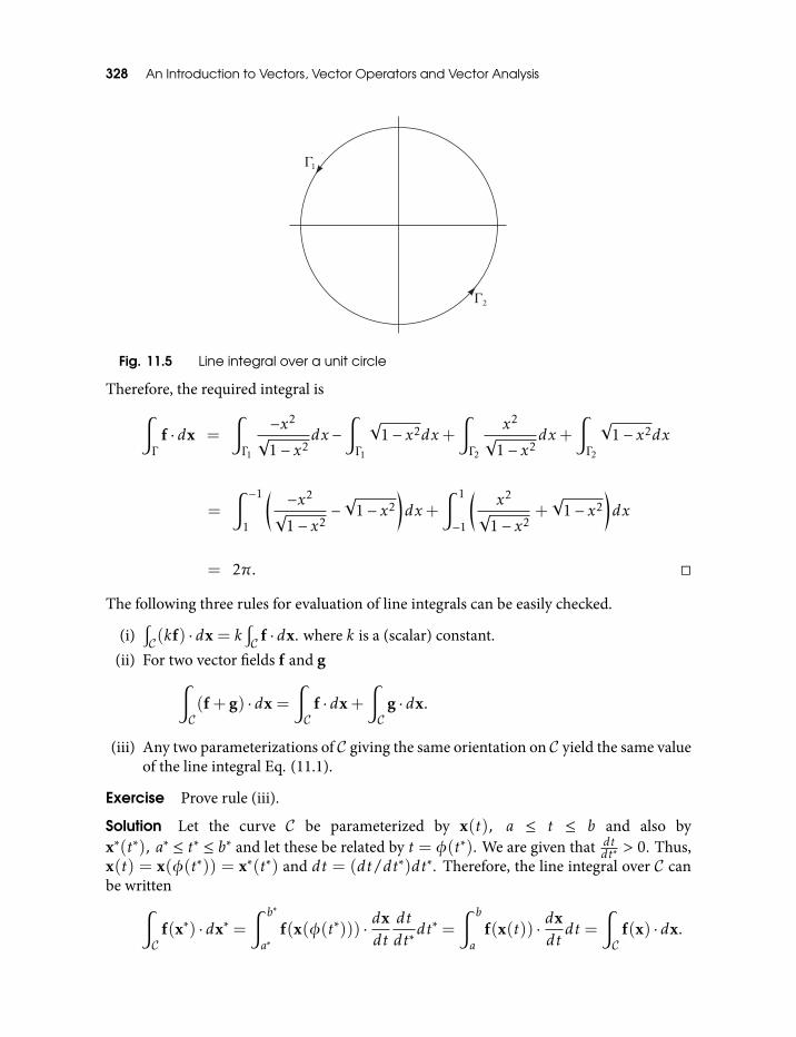
328 An Introduction to Vectors, Vector Operators and Vector Analysis
Fig. 11.5 Line integral over a unit circle
Therefore, the required integral is∫Γ
f · dx =
∫Γ1
−x2√
1− x2dx −
∫Γ1
√1− x2dx+
∫Γ2
x2√
1− x2dx+
∫Γ2
√1− x2dx
=
∫ −1
1
(−x2√
1− x2−√
1− x2
)dx+
∫ 1
−1
(x2
√1− x2
+√
1− x2
)dx
= 2π.
The following three rules for evaluation of line integrals can be easily checked.
(i)∫C(kf) · dx = k
∫C f · dx. where k is a (scalar) constant.
(ii) For two vector fields f and g∫C(f+ g) · dx =
∫C
f · dx+∫C
g · dx.
(iii) Any two parameterizations of C giving the same orientation on C yield the same valueof the line integral Eq. (11.1).
Exercise Prove rule (iii).
Solution Let the curve C be parameterized by x(t), a ≤ t ≤ b and also byx∗(t∗), a∗ ≤ t∗ ≤ b∗ and let these be related by t = φ(t∗). We are given that dt
dt∗ > 0. Thus,x(t) = x(φ(t∗)) = x∗(t∗) and dt = (dt/dt∗)dt∗. Therefore, the line integral over C canbe written∫
Cf(x∗) · dx∗ =
∫ b∗
a∗f(x(φ(t∗))) · dx
dtdtdt∗
dt∗ =
∫ b
af(x(t)) · dx
dtdt =
∫C
f(x) · dx.
Vector Integration 329
Note that f(x(t)) and f(x(φ(t∗))) are different functions of their arguments but theirvalues match at t and t∗ satisfying t = φ(t∗), both corresponding to the same point P onthe curve of integration.
We now give two results often used while evaluating line integrals. Let i, j, k be anorthonormal basis and x,y,z be the corresponding Cartesian coordinate system. Let avector field f(x) have components f1,2,3(x) along i, j, k respectively and let Γ be somesmooth curve in space.
(i) We can write∫Γ
f(x) · dx =
∫Γ
(f1(x)i+ f2(x)j+ f3(x)k) · (dxi+ dy j+ dzk)
=
∫Γ
f1(x)dx+∫Γ
f2(x)dy+∫Γ
f3(x)dz (11.6)
where we have used the orthonormality of the basis. Thus, a line integral over a vectorfield along a curve Γ is the sum of the line integrals over the components of the fieldalong Γ .
Exercise Integrate the field
f(x) = x2y2i+ y j+ zyk
along the curve y2 = 4x from (0,0) to (4,4).
Solution Note that the curve is on the xy plane and z = 0 = dz along the curve.We have,∫
Γ
f(x) · dx =
∫Γ
(x2y2i+ y j) · (dxi+ dy j)
=
∫Γ
x2y2dx+
∫Γ
ydy
Along the curve, y2 = 4x so that∫Γ
x2y2dx =
∫ 4
04x3dx = 256
and ∫ 4
0ydy = 8.
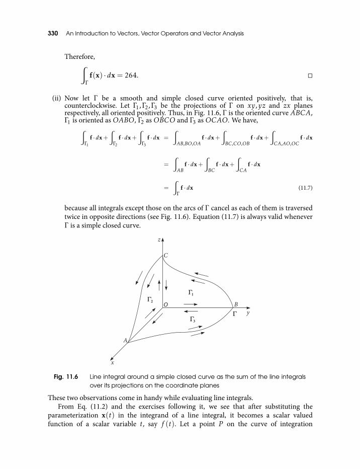
330 An Introduction to Vectors, Vector Operators and Vector Analysis
Therefore,∫Γ
f(x) · dx = 264.
(ii) Now let Γ be a smooth and simple closed curve oriented positively, that is,counterclockwise. Let Γ1,Γ2,Γ3 be the projections of Γ on xy,yz and zx planesrespectively, all oriented positively. Thus, in Fig. 11.6, Γ is the oriented curve ABCA,Γ1 is oriented asOABO, Γ2 asOBCO and Γ3 asOCAO. We have,∫
Γ1
f ·dx+∫Γ2
f ·dx+∫Γ3
f ·dx =
∫AB,BO,OA
f ·dx+∫BC,CO,OB
f ·dx+∫CA,AO,OC
f ·dx
=
∫AB
f · dx+∫BC
f · dx+∫CA
f · dx
=
∫Γ
f · dx (11.7)
because all integrals except those on the arcs of Γ cancel as each of them is traversedtwice in opposite directions (see Fig. 11.6). Equation (11.7) is always valid wheneverΓ is a simple closed curve.
Fig. 11.6 Line integral around a simple closed curve as the sum of the line integralsover its projections on the coordinate planes
These two observations come in handy while evaluating line integrals.From Eq. (11.2) and the exercises following it, we see that after substituting the
parameterization x(t) in the integrand of a line integral, it becomes a scalar valuedfunction of a scalar variable t, say f (t). Let a point P on the curve of integration
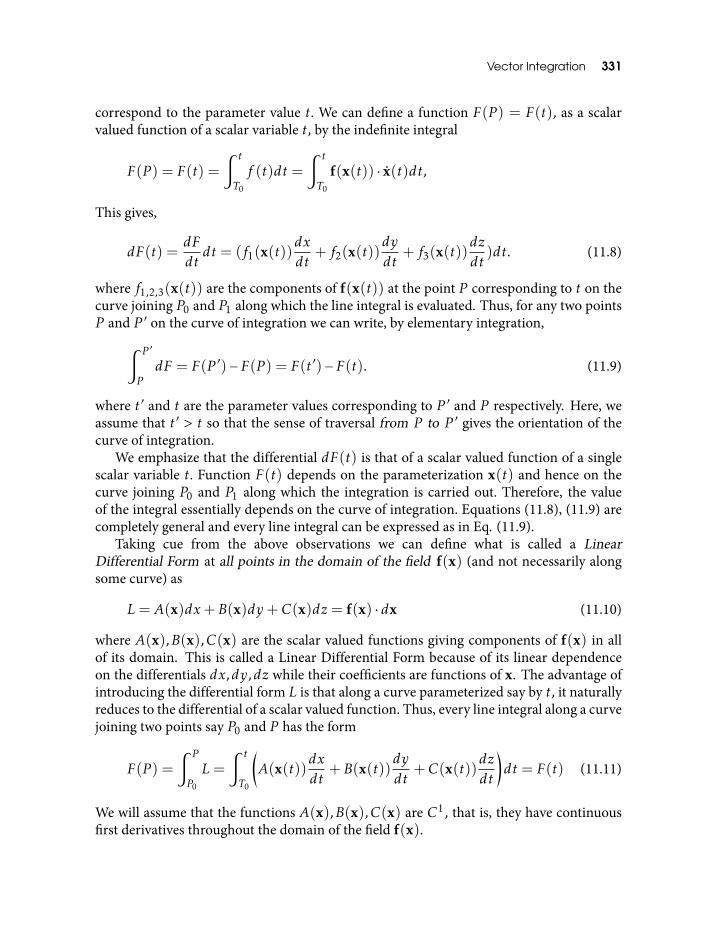
Vector Integration 331
correspond to the parameter value t. We can define a function F(P ) = F(t), as a scalarvalued function of a scalar variable t, by the indefinite integral
F(P ) = F(t) =
∫ t
T0
f (t)dt =
∫ t
T0
f(x(t)) · x(t)dt,
This gives,
dF(t) =dFdtdt = (f1(x(t))
dxdt
+ f2(x(t))dy
dt+ f3(x(t))
dzdt
)dt. (11.8)
where f1,2,3(x(t)) are the components of f(x(t)) at the point P corresponding to t on thecurve joining P0 and P1 along which the line integral is evaluated. Thus, for any two pointsP and P ′ on the curve of integration we can write, by elementary integration,∫ P ′
PdF = F(P ′)−F(P ) = F(t′)−F(t). (11.9)
where t′ and t are the parameter values corresponding to P ′ and P respectively. Here, weassume that t′ > t so that the sense of traversal from P to P ′ gives the orientation of thecurve of integration.
We emphasize that the differential dF(t) is that of a scalar valued function of a singlescalar variable t. Function F(t) depends on the parameterization x(t) and hence on thecurve joining P0 and P1 along which the integration is carried out. Therefore, the valueof the integral essentially depends on the curve of integration. Equations (11.8), (11.9) arecompletely general and every line integral can be expressed as in Eq. (11.9).
Taking cue from the above observations we can define what is called a LinearDifferential Form at all points in the domain of the field f(x) (and not necessarily alongsome curve) as
L= A(x)dx+B(x)dy+C(x)dz = f(x) · dx (11.10)
where A(x),B(x),C(x) are the scalar valued functions giving components of f(x) in allof its domain. This is called a Linear Differential Form because of its linear dependenceon the differentials dx,dy,dz while their coefficients are functions of x. The advantage ofintroducing the differential form L is that along a curve parameterized say by t, it naturallyreduces to the differential of a scalar valued function. Thus, every line integral along a curvejoining two points say P0 and P has the form
F(P ) =
∫ P
P0
L=
∫ t
T0
(A(x(t))
dxdt
+B(x(t))dy
dt+C(x(t))
dzdt
)dt = F(t) (11.11)
We will assume that the functions A(x),B(x),C(x) are C1, that is, they have continuousfirst derivatives throughout the domain of the field f(x).
332 An Introduction to Vectors, Vector Operators and Vector Analysis
We are interested in finding out the class of fields, the value of whose line integraldepends only on the end points irrespective of the curve joining the end points used toevaluate the integral. This happens when the field is conservative, that is, the field is thegradient of a potential φ(x) so that
f(x) = ∇φ(x)
at all points at which f(x) is defined. Then using Eq. (10.27) we can write∫C
f(x)·dx =
∫ T2
T1
∇φ(x(t))·x(t)dt =∫ T2
T1
dφ
dtdt = φ(x(t))
∣∣∣∣T2T1
= φ(P1)−φ(P0).
Thus, if the field is the gradient of a potential, then its line integral depends only on thevalues of the potential at the end points, independent of the curve joining the end points.
It turns out that the reverse implication is also true. That is, a vector field whose lineintegral over a smooth arc joining any two points in its domain depends only on its endpoints then it must be conservative, that is, it must be the gradient of some scalar fieldφ(x). A vector field being the gradient of some scalar field is equivalent to its linear formbeing a perfect differential, that is, there is a scalar valued function φ(x) satisfying
L= f · dx = ∇φ(x) · dx =∂φ(x)∂x
dx+∂φ(x)∂y
dy+∂φ(x)∂z
dz = dφ. (11.12)
Note that we require this equation to be valid at every point in the domain of f and notonly at the points on some curve in the domain. The RHS of Eq. (11.12) is easilyrecognized as the differential dφ of the scalar valued function φ. Now assume that theline integral of f over some smooth oriented arc Γ depends only on the end points of Γ .We want to show that there is a scalar function φ(x) defined on the domain of f such thatdφ = L where L = A(x)dx+ B(x)dy +C(x)dz is the linear differential form giving theintegrand of the line integral. Without losing generality we can assume that any two pointsin the domain can be connected by a smooth oriented arc. We fix a point P0 in the domainand define the function φ(x) = φ(P ) at any point P as the value of the line integral overany smooth oriented (from P0 to P ) curve joining P0 and P . To get the partial derivativesof φ consider any point (x,y,z) ≡ P and a smooth oriented curve, say Γ , joining P0 and P .Since the domain is an open set, all points (x+∆x,y,z) = P ′ are in the domain, provided|∆x| is sufficiently small. Let γ be the oriented straight line segment joining P and P ′ (seeFig. 11.7). We can arrange, without losing generality, that the curve Γ + γ is a simpleoriented polygonal arc without any knots and overlaps with initial point P0 and final pointP ′ . It follows, then, by Eq. (11.5) that
φ(x+∆x,y,z)−φ(x,y,z) = φ(P ′)−φ(P ) =∫Γ+γ
L−∫Γ
L=
∫γL
=
∫ x+∆x
xA(t,y,z)dt = A(x,y,z)∆x (11.13)
Vector Integration 333
Dividing by ∆x and passing to the limit as ∆x→ 0 we find that
∂φ
∂x= A
and similarly, ∂φ∂y = B and ∂φ∂z = C. This shows that dφ = L as we wanted.
Fig. 11.7 Illustrating Eq. (11.13)
Exercise Show that a vector field is conservative, if and only if its line integral over everyclosed loop is zero.
We have proved that the conservative property of a vector field and dependence of its lineintegral only on the end points of the curve of integration are equivalent. However, thisresult is not of much practical value unless we find out some independent criteria todetermine whether a given vector field is conservative or not. Equivalently, we have to findout whether a given differential form L is a perfect differential or not, that is, whetherthere is a function φ(x) satisfying L= ∇φ · dx.
The necessary condition for a vector field to be conservative is that its curl vanisheseverywhere in its domain. Since the field is given to be conservative, we have,
∇× f(x) = ∇×∇φ(x) = 0 (11.14)
for all x in the domain of f(x) because we have shown before that the curl of a gradient isalways zero (see Eq. (10.90)). It is useful to state this necessary condition in terms of thelinear differential form which, for a conservative field, ought to be a perfect differential:
L= A(x)dx+B(x)dy+C(x)dz = ∇φ(x) · dx =∂φ
∂xdx+
∂φ
∂ydy+
∂φ
∂zdz,
which means,
A=∂φ
∂x, B=
∂φ
∂yC =
∂φ
∂z.
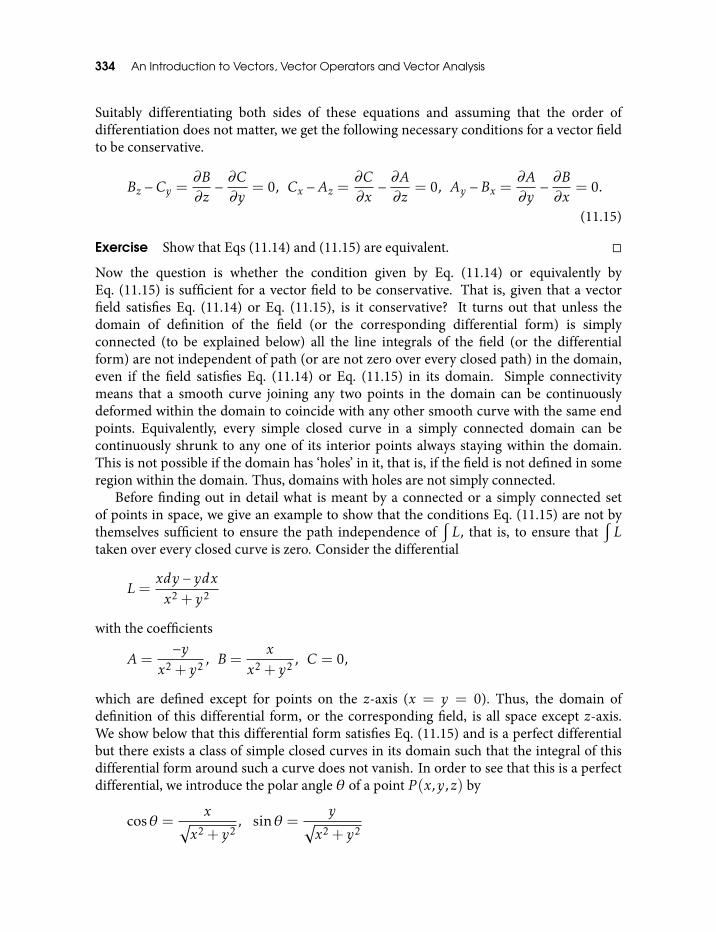
334 An Introduction to Vectors, Vector Operators and Vector Analysis
Suitably differentiating both sides of these equations and assuming that the order ofdifferentiation does not matter, we get the following necessary conditions for a vector fieldto be conservative.
Bz −Cy =∂B∂z− ∂C∂y
= 0, Cx −Az =∂C∂x− ∂A∂z
= 0, Ay −Bx =∂A∂y− ∂B∂x
= 0.
(11.15)
Exercise Show that Eqs (11.14) and (11.15) are equivalent.
Now the question is whether the condition given by Eq. (11.14) or equivalently byEq. (11.15) is sufficient for a vector field to be conservative. That is, given that a vectorfield satisfies Eq. (11.14) or Eq. (11.15), is it conservative? It turns out that unless thedomain of definition of the field (or the corresponding differential form) is simplyconnected (to be explained below) all the line integrals of the field (or the differentialform) are not independent of path (or are not zero over every closed path) in the domain,even if the field satisfies Eq. (11.14) or Eq. (11.15) in its domain. Simple connectivitymeans that a smooth curve joining any two points in the domain can be continuouslydeformed within the domain to coincide with any other smooth curve with the same endpoints. Equivalently, every simple closed curve in a simply connected domain can becontinuously shrunk to any one of its interior points always staying within the domain.This is not possible if the domain has ‘holes’ in it, that is, if the field is not defined in someregion within the domain. Thus, domains with holes are not simply connected.
Before finding out in detail what is meant by a connected or a simply connected setof points in space, we give an example to show that the conditions Eq. (11.15) are not bythemselves sufficient to ensure the path independence of
∫L, that is, to ensure that
∫L
taken over every closed curve is zero. Consider the differential
L=xdy − ydxx2 + y2
with the coefficients
A=−y
x2 + y2 , B=x
x2 + y2 , C = 0,
which are defined except for points on the z-axis (x = y = 0). Thus, the domain ofdefinition of this differential form, or the corresponding field, is all space except z-axis.We show below that this differential form satisfies Eq. (11.15) and is a perfect differentialbut there exists a class of simple closed curves in its domain such that the integral of thisdifferential form around such a curve does not vanish. In order to see that this is a perfectdifferential, we introduce the polar angle θ of a point P (x,y,z) by
cosθ =x√
x2 + y2, sinθ =
y√x2 + y2
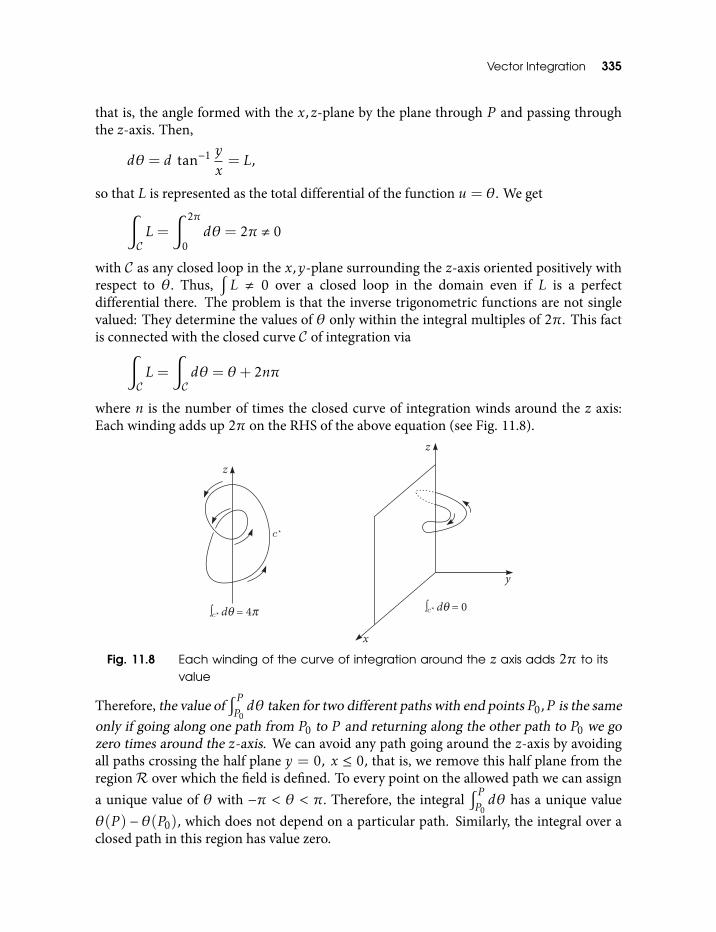
Vector Integration 335
that is, the angle formed with the x,z-plane by the plane through P and passing throughthe z-axis. Then,
dθ = d tan−1 y
x= L,
so that L is represented as the total differential of the function u = θ. We get∫CL=
∫ 2π
0dθ = 2π , 0
with C as any closed loop in the x,y-plane surrounding the z-axis oriented positively withrespect to θ. Thus,
∫L , 0 over a closed loop in the domain even if L is a perfect
differential there. The problem is that the inverse trigonometric functions are not singlevalued: They determine the values of θ only within the integral multiples of 2π. This factis connected with the closed curve C of integration via∫
CL=
∫Cdθ = θ+ 2nπ
where n is the number of times the closed curve of integration winds around the z axis:Each winding adds up 2π on the RHS of the above equation (see Fig. 11.8).
Fig. 11.8 Each winding of the curve of integration around the z axis adds 2π to itsvalue
Therefore, the value of∫ PP0dθ taken for two different paths with end points P0,P is the same
only if going along one path from P0 to P and returning along the other path to P0 we gozero times around the z-axis. We can avoid any path going around the z-axis by avoidingall paths crossing the half plane y = 0, x ≤ 0, that is, we remove this half plane from theregionR over which the field is defined. To every point on the allowed path we can assigna unique value of θ with −π < θ < π. Therefore, the integral
∫ PP0dθ has a unique value
θ(P ) − θ(P0), which does not depend on a particular path. Similarly, the integral over aclosed path in this region has value zero.
336 An Introduction to Vectors, Vector Operators and Vector Analysis
Simply connected sets
An open set R in space is said to be connected if every pair P0,P1 of distinct points init can be connected by a smooth arc wholly within R. Such an arc is parameterized bya triplet of continuously differentiable functions (x(t),y(t),z(t)), 0 ≤ t ≤ 1 ; the pointP (t) = (x(t),y(t),z(t)) lies in R for all t, coincides with P0 for t = 0 and with P1 fort = 1. Obviously, in a connected set, any two points can also be joined by a path comprisinga string of smooth arcs joined at their end points.
Examples of connected sets are the convex sets R any two of whose points P ′ and P ′′can be joined by a line segment inR. The corresponding linear paths joining P ′(x′,y′,z′)and P ′′(x′′,y′′,z′′) are simply the triple of linear functions
x(t) = (1− t)x′ + tx′′ y(t) = (1− t)y′ + ty′′ z(t) = (1− t)z′ + tz′′
for 0 ≤ t ≤ 1.Examples of convex sets are solid spheres or cubes. Examples of connected but not
convex sets are solid torus, a spherical shell (space between two concentric spheres) andthe outside of a sphere or cylinder. A set R which is not connected consists of connectedsubsets called the components of R. Examples of disconnected sets are the set of pointsnot belonging to a spherical shell, or a set of points none of whose coordinates areintegers.
Now let C0 and C1 be any two paths in R, given by (x0(t),y0(t),z0(t)) and(x1(t),y1(t),z1(t)) respectively. Let their end points P ′ and P ′′, corresponding to t = 0and t = 1 respectively, be the same. The connected set R is simply connected, if we candeform C0 into C1 by means of a continuous family of paths Cλ with common end pointsP ′,P ′′ . This means that there exist continuous functions (x(t,λ),y(t,λ),z(t,λ)) of thetwo variables t,λ for 0 ≤ t ≤ 1, 0 ≤ λ ≤ 1 such that the point P (t,λ) = (x(t,λ),y(t,λ),z(t,λ)) always lies inR and such that P (t,λ = 0) coincides with P (t) = (x0(t),y0(t),z0(t)), P (t,λ = 1) coincides with P (t) = (x1(t),y1(t),z1(t)), P (t = 0,λ)coincides with P ′ and P (t = 1,λ) coincides with P ′′ . For each fixed λ the functions(x(t,λ), y(t,λ),z(t,λ)) determine a path Cλ in R that joins the end points P ′ and P ′′ .As λ varies from 0 to 1, the path Cλ changes continuously from C0 to C1. This defines the“continuous deformation” of C0 into C1 (see Fig. 11.9).
As can be easily seen, convex sets are simply connected. The family of curves Cλcontinuously deforming C0 to C1, all curves with common end points P ′,P ′′, is given by
x(t,λ) = (1−λ)x0(t) +λx1(t),
y(t,λ) = (1−λ)y0(t) +λy1(t),
z(t,λ) = (1−λ)z0(t) +λz1(t).
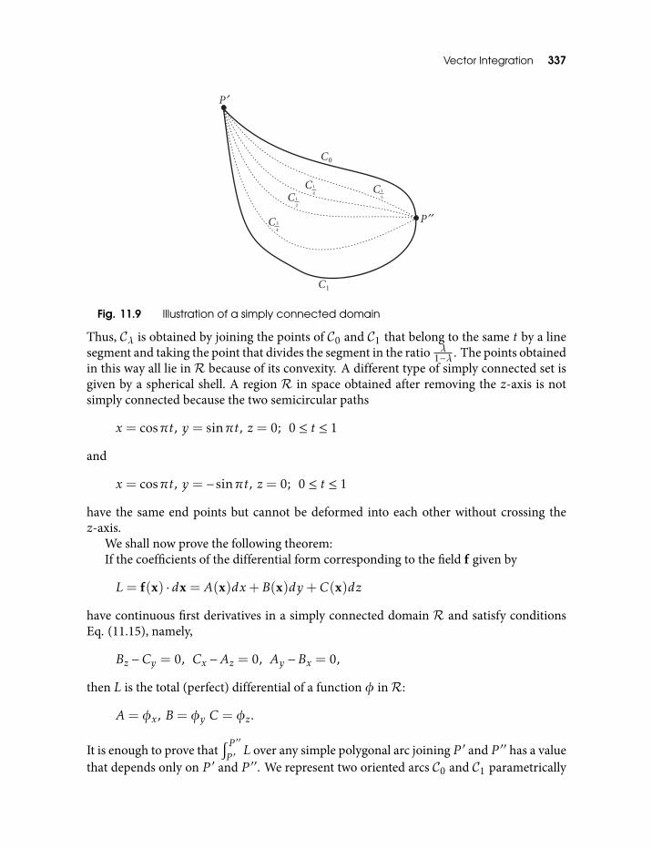
Vector Integration 337
Fig. 11.9 Illustration of a simply connected domain
Thus, Cλ is obtained by joining the points of C0 and C1 that belong to the same t by a linesegment and taking the point that divides the segment in the ratio λ
1−λ . The points obtainedin this way all lie in R because of its convexity. A different type of simply connected set isgiven by a spherical shell. A region R in space obtained after removing the z-axis is notsimply connected because the two semicircular paths
x = cosπt, y = sinπt, z = 0; 0 ≤ t ≤ 1
and
x = cosπt, y = −sinπt, z = 0; 0 ≤ t ≤ 1
have the same end points but cannot be deformed into each other without crossing thez-axis.
We shall now prove the following theorem:If the coefficients of the differential form corresponding to the field f given by
L= f(x) · dx = A(x)dx+B(x)dy+C(x)dz
have continuous first derivatives in a simply connected domain R and satisfy conditionsEq. (11.15), namely,
Bz −Cy = 0, Cx −Az = 0, Ay −Bx = 0,
then L is the total (perfect) differential of a function φ inR:
A= φx, B= φy C = φz.
It is enough to prove that∫ P ′′P ′L over any simple polygonal arc joining P ′ and P ′′ has a value
that depends only on P ′ and P ′′ . We represent two oriented arcs C0 and C1 parametrically
338 An Introduction to Vectors, Vector Operators and Vector Analysis
by (x0(t),y0(t),z0(t)) and (x1(t),y1(t),z1(t)), 0 ≤ t ≤ 1 respectively with t = 0 yieldingP ′ and t = 1 yielding P ′′ . Using the simple connectivity of R we can imbed paths C0and C1 into a continuous family (x(t,λ),y(t,λ),z(t,λ)) reducing to (x0(t),y0(t),z0(t))and (x1(t),y1(t),z1(t)) for λ = 0,1 respectively and to P ′,P ′′ for t = 0,1 respectively.We have, for the integral around the loop,∫
C1
L−∫C0
L=
∫ 1
0[(Axt +Byt +Czt)
∣∣∣λ=1 − (Axt +Byt +Czt)∣∣∣λ=0
]dt,
where (x,y,z) are the functions of t,λ forming the continuous family of paths. We assumethat these functions have continuous first and mixed second derivatives with respect to tand λ for 0 ≤ t ≤ 1 and 0 ≤ λ ≤ 1. Then by elementary integration,∫
C1
L−∫C0
L=
∫ 1
0dt
∫ 1
0(Axt +Byt +Czt)λdλ.
Now, using the chain rule and the conditions Eq. (11.15) we get the identity
(Axt +Byt +Czt)λ = Axλt +Byλt +Czλt +Axxλxt +Ayyλxt +Azzλxt
+Bxxλyt +Byyλyt +Bzzλyt +Cxxλzt +Cyyλzt +Czzλzt
= (Axλ+Byλ+Czλ)t (11.16)
Interchanging orders of integration we find∫C1
L−∫C0
L=
∫ 1
0dλ
∫ 1
0(Axλ+Byλ+Czλ)tdt = 0,
since xλ,yλ,zλ vanish for t = 0,1 because the end points are independent of λ. Thiscompletes the proof.
We see the important part played by the assumption that the region R is simplyconnected: It enables us to convert the difference of the line integrals into a double integralover some intermediate region. The above proof can be extended to the case where theintermediate paths are continuous but may not be differentiable with respect to λ and alsoto the case where C0 and C1 are only sectionally smooth, that is, polygonal arcs.
Exercise Find out whether the field f(x) = exy i+ ex+y j is conservative.
Solution The coefficients in the linear form are A(x,y) = exy and B(x,y) = ex+y andconditions Eq. (11.15) reduce to ∂A
∂y = ∂B∂x . Evaluating both sides we see that they are not
equal. Hence, the field is not conservative.
Exercise Find whether the following fields are conservative.
Vector Integration 339
(i) f(x) = cosy i− x siny j− coszk.
(ii) f(x) = xy i+ (x2 + y2)j.
(iii) f(x) = (x2 − y2)i+ xy j.
Hint Directly evaluate ∇× f.
Exercise Let the field be f(x) = 2xy i + (x2 + 3y2)j. Find whether the field isconservative and if it is, find the potential function.
Solution Evaluating Ay and Bx we find that they are equal, so the potential function say
φ(x,y) may exist. To find it, we first evaluate the integral∫A(x,y) dx =
∫ ∂φ∂x dx =∫
2xydx keeping y constant to get x2y for the indefinite integral. We must now find afunction u(y) such that
∂∂y
(x2y+ u(y)) = x2 + 3y2.
Differentiating and simplifying, this equation leads to
dudy
= 3y2.
Integrating, we find u(y) = y3. This gives, for the potential function,
φ(x,y) = x2y+ y3.
Exercise Show that f(x) = (siny + z)i − (xcosy − z)j − (x − y)k is conservative andfind the function φ such that f(x) = ∇φ.
Solution We check that ∇× f = 0 so that this field is conservative.To find a potential φ we equate the components of f = ∇φ. We get
(i) fx =∂φ∂x = siny+ z,
(ii) fy =∂φ∂y = xcosy − z,
(iii) fz =∂φ∂z = x − y.
Integrating fx,fy ,fz with respect to x,y,z respectively, we obtain
(iv) φ = x siny+ xz+ f (y,z),
(v) φ = x siny − yz+ g(x,z),
(vi) φ = xz − yz+ h(x,y).
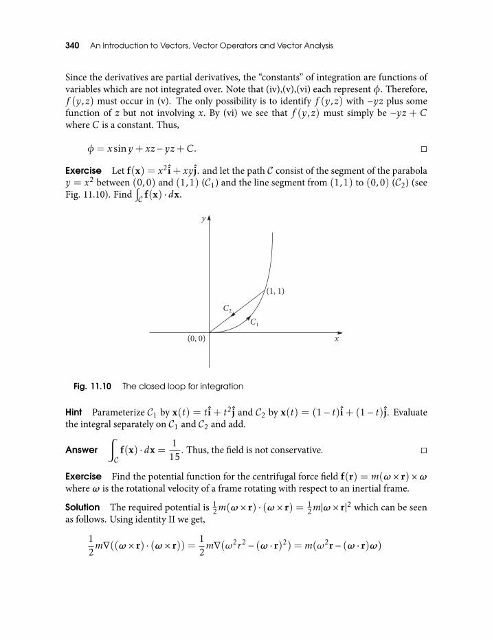
340 An Introduction to Vectors, Vector Operators and Vector Analysis
Since the derivatives are partial derivatives, the “constants” of integration are functions ofvariables which are not integrated over. Note that (iv),(v),(vi) each represent φ. Therefore,f (y,z) must occur in (v). The only possibility is to identify f (y,z) with −yz plus somefunction of z but not involving x. By (vi) we see that f (y,z) must simply be −yz + Cwhere C is a constant. Thus,
φ = x siny+ xz − yz+C.
Exercise Let f(x) = x2i+ xy j. and let the path C consist of the segment of the parabolay = x2 between (0,0) and (1,1) (C1) and the line segment from (1,1) to (0,0) (C2) (seeFig. 11.10). Find
∫C f(x) · dx.
Fig. 11.10 The closed loop for integration
Hint Parameterize C1 by x(t) = ti + t2j and C2 by x(t) = (1 − t)i + (1 − t)j. Evaluatethe integral separately on C1 and C2 and add.
Answer∫C
f(x) · dx =1
15. Thus, the field is not conservative.
Exercise Find the potential function for the centrifugal force field f(r) = m(ω × r) ×ωwhere ω is the rotational velocity of a frame rotating with respect to an inertial frame.
Solution The required potential is 12m(ω × r) · (ω × r) = 1
2m|ω × r|2 which can be seenas follows. Using identity II we get,
12m∇((ω × r) · (ω × r)) =
12m∇(ω2r2 − (ω · r)2) =m(ω2r− (ω · r)ω)
Vector Integration 341
which, using identity I reduces to
12m∇((ω × r) · (ω × r)) =mω × (r×ω) =m(ω × r)×ω.
In general, a vector field is produced by given sources and the relation between the fieldsand their sources is formulated in terms of a system of differential equations in which thesources are given and the fields are the solutions of these differential equations. The mostcelebrated examples are the Maxwell’s equations giving electric and magnetic fieldsproduced by the given distributions of charges and currents and the Navier–Stokesequations giving velocity field of an imperfect fluid for given distribution of pressure,viscosity, shear, external forces etc. For the conservative fields these differential equationscan be transformed into equations for the potential, which are easier to handle, as theydeal with scalar fields. For example, the equation for the electrostatic field ∇ · E = ρ/ε0gets transformed to Poisson’s equation ∇2φ = −ρ/ε0 where φ is the electrostaticpotential satisfying E = −∇φ.
11.1.1 Curl of a vector field and the line integral
We express the curl of a vector field f(x) in terms of its line integral over a simple closedcurve Γ in a plane with unit normal n. Let S be the (planar) area enclosed by Γ and P be apoint interior to or on Γ . We define a number Gn by
Gn = limΓ→P
1S
∫Γ
f(x) · dx
where the integration is taken in the positive (counterclockwise) sense. Note that, ingeneral, this integral depends on the direction n because if we change n (by rotating theplane say) the integrand and hence the integral will change. The limit Γ → P requires thatevery point of Γ approaches P . If this limit exists, then Gn is independent of Γ . As we showbelow, if Γ is a planar curve and f(x) has Taylor series expansion around P , then the limitexists and is independent of Γ .
We choose the origin at P and let a point on Γ have position vector x relative to theorigin at P . We expand f(x) around P that is, around 0. We get
f(x) = f(0) + x · ∇f(0) +R, (11.17)
where R is the remainder containing all the second and higher order terms (x · ∇)2 · · · (seeEq. (10.22)). We set up a rectangular Cartesian coordinate system (ξ,η,ζ) with its originat P such that (ξ,η) plane contains Γ (see Fig. 11.11). The vector x has the components(ξ,η,ζ) and let the components of f(x) be fξ(x),fη(x),fζ(x). This gives
x · ∇fξ(x) = ξ∂fξ∂ξ
+ η∂fξ∂η
+ ζ∂fξ∂ζ
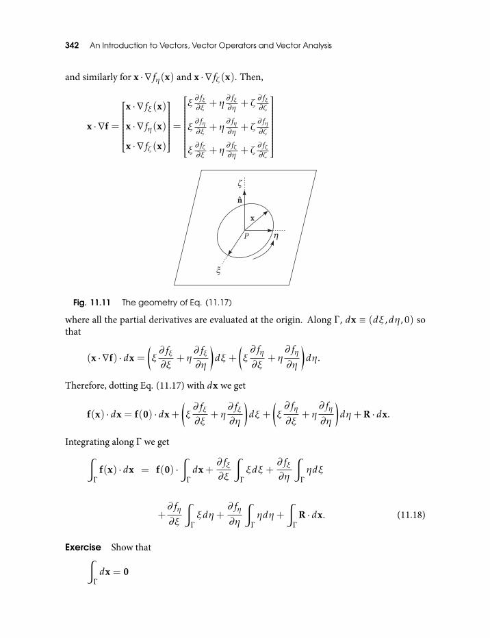
342 An Introduction to Vectors, Vector Operators and Vector Analysis
and similarly for x · ∇fη(x) and x · ∇fζ(x). Then,
x · ∇f =
x · ∇fξ(x)
x · ∇fη(x)
x · ∇fζ(x)
=ξ∂fξ∂ξ + η
∂fξ∂η + ζ
∂fξ∂ζ
ξ∂fη∂ξ + η
∂fη∂η + ζ
∂fη∂ζ
ξ∂fζ∂ξ + η
∂fζ∂η + ζ
∂fζ∂ζ
Fig. 11.11 The geometry of Eq. (11.17)
where all the partial derivatives are evaluated at the origin. Along Γ , dx ≡ (dξ,dη,0) sothat
(x · ∇f) · dx =
(ξ∂fξ∂ξ
+ η∂fξ∂η
)dξ +
(ξ∂fη∂ξ
+ η∂fη∂η
)dη.
Therefore, dotting Eq. (11.17) with dx we get
f(x) · dx = f(0) · dx+(ξ∂fξ∂ξ
+ η∂fξ∂η
)dξ +
(ξ∂fη∂ξ
+ η∂fη∂η
)dη+R · dx.
Integrating along Γ we get∫Γ
f(x) · dx = f(0) ·∫Γ
dx+∂fξ∂ξ
∫Γ
ξdξ +∂fξ∂η
∫Γ
ηdξ
+∂fη∂ξ
∫Γ
ξdη+∂fη∂η
∫Γ
ηdη+
∫Γ
R · dx. (11.18)
Exercise Show that∫Γ
dx = 0
Vector Integration 343
∫Γ
ξdξ = 0 = −∫Γ
ηdξ
and ∫Γ
ξdη = −∫Γ
ηdξ = S
where S is the area enclosed by Γ .
Thus, Eq. (11.18) reduces to (Fig. 11.11)
1S
∫Γ
f(x) · dx =
(∂fη∂ξ−∂fξ∂η
)+
1S
∫Γ
R · dx. (11.19)
In the last term the integral is of the order of |x|3 as R is of the order of |x|2. Therefore, thelast term is of the order of |x| and vanishes in the limit Γ → P or |x| → 0. Therefore,
Gn = limΓ→P
1S
∫Γ
f(x) · dx =∂fη∂ξ−∂fξ∂η
This limit depends only on the derivatives of f evaluated at P and is independent of Γ .Now let Γ be a planar curve in a plane defined by the normal direction n and let Γ1,Γ2,Γ3
be the projections of Γ on the xy,yz,zx planes of the coordinate system corresponding toan orthonormal basis (i, j, k). We know that (see Eq. (11.11)),∫
Γ
f · dx =
∫Γ1
f · dx+∫Γ2
f · dx+∫Γ3
f · dx.
The areas of projections are given by
S1 = S i · n S2 = S j · n S3 = Sk · n
where i · n etc are the direction cosines of n. Hence,
1S
∫Γ
f(x) · dx =i · nS1
∫Γ1
f(x) · dx+j · nS2
∫Γ2
f(x) · dx+k · nS3
∫Γ3
f(x) · dx.
In the limit as Γ → P we get,
Gn = G′ · n
where
G′ = G′1i+G′2j+G′3k
344 An Introduction to Vectors, Vector Operators and Vector Analysis
and
G′i = limΓi→P
1Si
∫Γi
f(x) · dx i = 1,2,3.
For the components of G′ we get
G′1 = limΓ1→P
1S1
∫Γ1
f(x) · dx =∂fz∂y−∂fy∂z
G′2 = limΓ2→P
1S2
∫Γ2
f(x) · dx =∂fx∂z−∂fz∂x
G′3 = limΓ3→P
1S3
∫Γ3
f(x) · dx =∂fy∂x−∂fx∂y
.
We immediately identify G′ with curl f or ∇× f. Thus, the curl of a vector field that can beTaylor expanded around a point P can be approximated by its line integral around a simpleclosed curve Γ surrounding the point P . The approximation gets better as the size of Γ getssmaller but the quantitative estimate of the error will involve the field.
11.2 Applications of the Potential Functions
In this section we deal with the potential functions appearing in real life situations.1We obtain the gravitational field and the gravitational potential of a continuous body of
an arbitrary shape at a given point in space. From this, we obtain the internal and externalgravitational potential of a spherically symmetric body. We get the multipole expansion ofthe potential and the field of a body with arbitrary shape upto the first term correspondingto the deviation from sphericity. We do the same, upto third order term for an axiallysymmetric body.
Gravitational field due to a single particle of massm1 at x1 = x1(t) at a point x in spaceis given by
g1(x, t) = −Gm1x− x1(t)
|x− x1(t)|3. (11.20)
The particle at x1 = x1(t) is called the source of the field and the mass m1 is the sourcestrength. The field g1 is a map (actually a one parameter family) assigning a definite vectorg1(x, t) to every point x in space, at a given instant of time. Note that the time dependenceis solely due to the motion of the source.
1Both these applications are treated in [10] using geometric algebra.
Vector Integration 345
If a particle of massm is placed at a point x in the gravitational field g1, we say that thefield exerts a force
f1 = f(x, t) =mg1(x, t). (11.21)
Equation (11.21) is mathematically same as Newton’s force law. However, if we impartphysical reality to the field concept, it would mean that particles interact with each othervia their force fields rather than acting directly by exerting forces on one another inaccordance with Newton’s law. The gravitational field is regarded as a real physical entitypervading all space surrounding its source and acting on any matter that is present. Thefield concept also has a formal mathematical advantage. It enables us to separategravitational interactions into two parts, namely (a) production of gravitational fields byextended sources and (b) the effect of a given gravitational field on given bodies. We areconcerned here with the production of fields.
The single paticle gravitational field, Eq. (11.20), can be derived from the gravitationalpotential
φ1(x, t) =−Gm1
|x− x1(t)|, (11.22)
by differentiation, giving
g1(x, t) = −5xφ1(x, t), (11.23)
where 5x is the derivative (gradient) with respect to the field variable x. Henceforth, weleave suffix x to be understood. The gravitational potential energy of a particle with massm at x is given by
V1(x, t) =mφ1(x, t) =−Gmm1
|x− x1(t)|. (11.24)
It is important to clearly distinguish between potential and potential energy. Latter is theshared energy of two interacting objects, while former is characteristic of a single objectnamely its source.
The gravitational field g(x, t) of a N particle system is given by the superposition offields
g(x, t) =N∑k=1
gk(x, t) = −GN∑k=1
mkx− xk(t)|x− xk(t)|3
. (11.25)
A particle of massm at x experiences a force
f =mg =∑k
mgk =∑k
fk (11.26)
346 An Introduction to Vectors, Vector Operators and Vector Analysis
due to field in Eq. (11.25) which is consistent with the law of superposition of forces. Thisfield can be derived from a potential; thus
g(x, t) = −5φ(x, t) (11.27)
where
φ(x, t) =∑k
φk(x, t) = −G∑k
mk|x− xk(t)|
. (11.28)
The potential energy of a particle in a field is given by
V (x, t) =mφ(x, t). (11.29)
Note that this does not include the potential energy of interaction between the particlesproducing the field. The internal energy can be ignored as long as we are concerned onlywith the influence of the system on external objects.
The gravitational field of a continuous body is obtained from that of a system of Nparticles via the following limiting process. We divide the body into small parts which canbe regarded as particulate and in the limit of infinitely small subdivision the sum inEq. (11.25) becomes the integral,
g(x, t) = −G∫dm′
x− x′(t)|x− x′(t)|3
(11.30)
where dm′ = dm(x′, t) is the mass given by the differential of the mass distributionm(x′, t), supposed to be known. In other words, this is the mass of a small enoughcorpuscle at point x′ at time t. Similar limiting process for Eq. (11.28) gives us thegravitational potential of a continuous body
φ(x, t) = −G∫
dm′
|x− x′(t)|. (11.31)
Henceforth we shall not write the time dependence explicitly.Equation (11.27) applies with φ(x, t) given by Eq. (11.31) so that we find the field g by
differentiating Eq. (11.31).For a spherically symmetric mass distribution, the integral in Eq. (11.31) can be easily
evaluated. We place the origin at body’s centre of mass and denote the position vectors withrespect to the centre of mass by r and r′ instead of x and x′ which we use in the case of anexternal inertial frame (see Fig. 11.12).
A spherically symmetric mass density is a function of radial distance alone. Thus,
dm′ = ρ(r ′)r ′2dr ′dΩ (11.32)
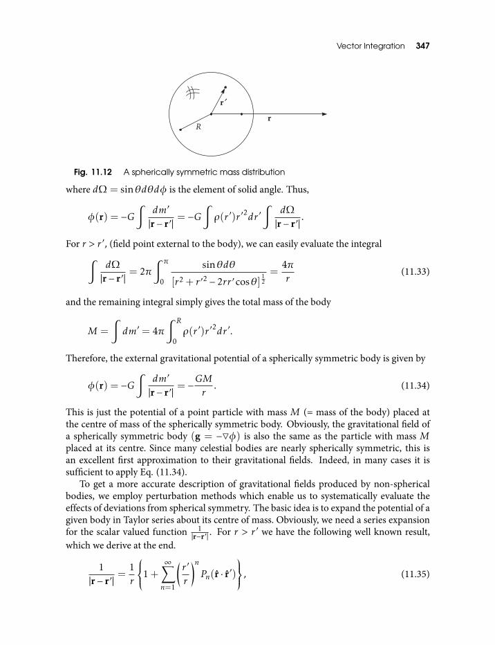
Vector Integration 347
Fig. 11.12 A spherically symmetric mass distribution
where dΩ= sinθdθdφ is the element of solid angle. Thus,
φ(r) = −G∫
dm′
|r− r′ |= −G
∫ρ(r ′)r ′2dr ′
∫dΩ|r− r′ |
.
For r > r ′, (field point external to the body), we can easily evaluate the integral∫dΩ|r− r′ |
= 2π∫ π
0
sinθdθ
[r2 + r ′2 − 2rr ′ cosθ]12=
4πr
(11.33)
and the remaining integral simply gives the total mass of the body
M =
∫dm′ = 4π
∫ R
0ρ(r ′)r ′2dr ′.
Therefore, the external gravitational potential of a spherically symmetric body is given by
φ(r) = −G∫
dm′
|r− r′ |= −GM
r. (11.34)
This is just the potential of a point particle with mass M (= mass of the body) placed atthe centre of mass of the spherically symmetric body. Obviously, the gravitational field ofa spherically symmetric body (g = −5φ) is also the same as the particle with mass Mplaced at its centre. Since many celestial bodies are nearly spherically symmetric, this isan excellent first approximation to their gravitational fields. Indeed, in many cases it issufficient to apply Eq. (11.34).
To get a more accurate description of gravitational fields produced by non-sphericalbodies, we employ perturbation methods which enable us to systematically evaluate theeffects of deviations from spherical symmetry. The basic idea is to expand the potential of agiven body in Taylor series about its centre of mass. Obviously, we need a series expansionfor the scalar valued function 1
|r−r′ | . For r > r ′ we have the following well known result,which we derive at the end.
1|r− r′ |
=1r
1+∞∑n=1
(r ′
r
)nPn(r · r′)
, (11.35)
348 An Introduction to Vectors, Vector Operators and Vector Analysis
where Pn are the Legender polynomials. A first few of these are
P1(r · r′) = r · r′
P2(r · r′) =12(3(r · r′)2 − 1)
P3(r · r′) =12(5(r · r′)3 − 3(r · r′)). (11.36)
A variant of Eq. (11.35) is
1|r− r′ |
=1r
1+∞∑n=1
r−2nPn(r · r′)
, (11.37)
where a first few Pn(r · r′) are
P1(r · r′) = r · r′
P2(r · r′) =12(3(r · r′)2 − r2r ′2)
P3(r · r′) =12(5(r · r′)3 − 3r2r ′2r · r′). (11.38)
It is clear from Eq. (11.35) that the magnitude of the nth term in the expansion is of theorder of ( r
′r )n so the series converges rapidly at a distance r which is large compared to the
dimensions of the body. Series (11.37) gives a series for the potential
φ(r) = −Gr
M +
1r2
∫P1(r · r′)dm′ +
1r4
∫P2(r · r′)dm′ + · · ·
By Eq. (11.38)∫
P1(r · r′)dm′ = r ·[∫
r′dm′]= r · [0] = 0.
Here,∫
r′dm′ gives the position vector of the centre of mass which vanishes because thecentre of mass is at the origin.
It is convenient to express the next term in the expansion (involving P2(r · r′)) in termsof the inertia operatorI : R3 7−→R3 or the moment of inertia tensor of the body, definedby, (Remember that I r ∈R3 is a vector),
I r =∫dm′r′ × (r× r′) =
∫dm′(r ′2r− (r′ · r)r′). (11.39)
Vector Integration 349
The trace of the inertia tensor is given by
T r I = 2∫dm′ r ′2 = I1 + I2 + I3, (11.40)
where I1, I2, I3 are the principal moments of inertia.
Exercise Prove Eq. (11.40).
Solution We set up the matrix representing the inertia operator in an orthonormal basisσ1,s2,s3 with elements Iij = σ i ·I σ j . Then, its trace is given by the sum of its diagonalelements. From Eq. (11.39) we get, suppressing primes,
3∑i=1
σ i ·I σ i =∫dm
3∑i=1
(r2 − r2i ) = 2
∫dmr2 = I1 + I2 + I3,
where I1, I2, I3 are the principal moments of inertia which are the eigenvalues of the inertiaoperator. The last equality follows because the trace is seen to be independent of the basisused to compute it.
Therefore,∫P2(r · r′)dm′ =
∫dm′
12(3(r · r′)2 − r2r ′2) =
12[r2T r I − 3r ·I r] =
12
r · Qr,
(11.41)
which defines a symmetric tensor
Qr = rT r I − 3I r. (11.42)
Exercise Show that the tensor Q is symmetric.
Solution We first show that the MI operator I is symmetric. We have, suppressingprimes,
Iij = σi ·I σj =∫dm(r2δij − rirj) = σj ·I σi = Iji .
This gives,
Qij = σ i · Qσ j = σ i · σ jT rI − 3σ i ·I σ j = Qji .
Following the well known terminology from electromagnetic theory, we call Q thegravitational quadrupole tensor. (Again, remember that LHS of Eq. (11.42) is a vectorin R3.)
350 An Introduction to Vectors, Vector Operators and Vector Analysis
Now the expanded potential is
φ(r) = −Gr
M +
12
r · Qrr4 + · · ·
. (11.43)
This is called a harmonic or multipole expansion of the potential. The quadrupole termdescribes the first non-zero correction to the potential of a spherically symmetric body.The gravitational field (g = −5φ) can be obtained from Eq. (11.43) with the help of
5(1
2r · Qr
)= Qr,
5rn = nrn−1r.
Thus,
g(r) = −Gr2
M r− 1
r2
(Qr− 5
2(r · Qr)r
)+ · · ·
. (11.44)
Exercise Derive Eq. (11.44).
This expression for the gravitational field holds for a body with arbitrary shape and densitydistribution.
The moment of inertia tensor for an axially symmetric body can be put in the form
I r = I1r+ (I3 − I1)(r · u)u, (11.45)
where I1 = I2 is the moment of inertia about any axis in the plane normal to the symmetryaxis and passing through the centre of mass, called equatorial moment of inertia, I3 is themoment of inertia about the symmetry axis, or the so called polar moment of inertia. u isthe direction of the symmetry axis.
Exercise Prove Eq. (11.45).
Solution Let σ1, σ2, u be the eigenbasis of the inertia operator of the axially symmetricbody and let r = r1σ1 + r2σ2 + r3u be a position vector. Due to symmetry about the axisgiven by u, the eigenvalues corresponding to σ1, σ2must be equal, giving the eigenvaluesto be I1, I1, I3. We get
I r = I1(r1σ1 + r2σ2) + I3r3u
= I1r+ I3r3u− I1r3u
= I1r+ (I3 − I1)(r · u)u.
Vector Integration 351
Then Eqs (11.42) and (11.40) give,
Qr = (I3 − I1)(r− 3(r · u)u). (11.46)
From Eq. (11.44), then, the gravitational field of an axially symmetric body is
g(r) = −MGr2
r+
32J2
(Rr
)2[1− 5(r · u)2 r+ 2r · u u] + · · ·
. (11.47)
where R is the equatorial radius of the body and J2 is defined as
J2 =I3 − I1MR2 . (11.48)
The constant J2 is a dimensionless measure of the oblateness of the body and the factor(Rr )
2 in Eq. (11.47) measures the rate at which the oblateness effect (on the field) falls offwith distance.
For an axially symmetric body, the effect of harmonics higher than the quadrupole arerather simply found, because the series Eq. (11.35) (or Eq. (11.37)) integrates to a harmonicexpansion for the potential, giving,
φ(r) = −GMr
1−∞∑n=2
Jn
(Rr
)nPn(r · u)
, (11.49)
where Jn are the dimensionless constant coefficients. As stated above, J2 measures theoblateness of the body and is related to the moment of inertia via Eq. (11.48). Theconstant J3 measures the extent to which the body is “pearshaped”, (i.e., the southernhemisphere fatter than the northern hemisphere). The advantage of Eq. (11.49) is that itcan be immediately written down once the axial symmetry is assumed and the constantsJn can be determined empirically, in particular, by fitting Eq. (11.49) to data on orbitingsatellites. For the earth,
J2 = 1.083× 10⁻³, J3 = −2.5× 10⁻⁶, J4 = −1.6× 10⁻⁶, J5 = −0.2× 10⁻⁶.
Clearly the quadrupole harmonic strongly dominates. The contributions of the harmonicsdecrease with n because of the factor
(Rr
)nin Eq. (11.49). Since Jn are dimensionless,
comparison of Jn values for different planets can be used to quantitatively compare theshapes of planets.
Using the directional derivative
u · 5r =u− (u · r)r
r, (11.50)
we can differentiate the term (n = 3) in Eq. (11.49) to get its contribution to thegravitational field as
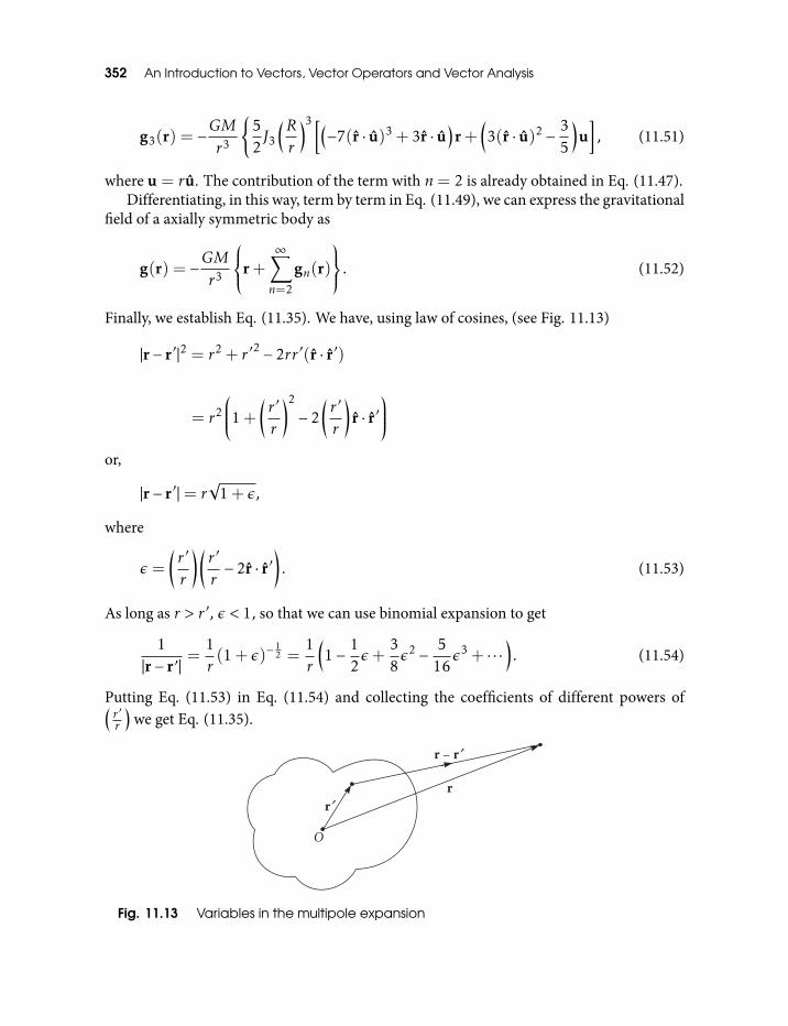
352 An Introduction to Vectors, Vector Operators and Vector Analysis
g3(r) = −GM
r3
52J3
(Rr
)3 [(−7(r · u)3 + 3r · u
)r+
(3(r · u)2 − 3
5
)u], (11.51)
where u = ru. The contribution of the term with n= 2 is already obtained in Eq. (11.47).Differentiating, in this way, term by term in Eq. (11.49), we can express the gravitational
field of a axially symmetric body as
g(r) = −GMr3
r+∞∑n=2
gn(r)
. (11.52)
Finally, we establish Eq. (11.35). We have, using law of cosines, (see Fig. 11.13)
|r− r′ |2 = r2 + r ′2 − 2rr ′(r · r′)
= r2
1+
(r ′
r
)2
− 2(r ′
r
)r · r′
or,
|r− r′ |= r√
1+ ε,
where
ε =
(r ′
r
)(r ′
r− 2r · r′
). (11.53)
As long as r > r ′, ε < 1, so that we can use binomial expansion to get
1|r− r′ |
=1r(1+ ε)−
12 =
1r
(1− 1
2ε+
38ε2 − 5
16ε3 + · · ·
). (11.54)
Putting Eq. (11.53) in Eq. (11.54) and collecting the coefficients of different powers of(r ′r
)we get Eq. (11.35).
Fig. 11.13 Variables in the multipole expansion
Vector Integration 353
Exercise Develop the multipole expansion for the electrostatic potential at r due to anarbitrary localized charge distribution, in powers of 1
r . This is analogous to the abovedevelopment of multipole expansion for the gravitational potential of an arbitrarylocalized mass distribution. Give the geometric interpretation of the of the termsproportional to 1
r2 , 1r3 , 1
r4 . Compare these two cases. (Consult ref [9]).
We shall now obtain the equation to the surface of the earth by assuming it to be anequipotential for the effective gravitational potential
Φ(r) = V (r)− 12(Ω× r)2, (11.55)
where V (r) is the true gravitational potential at the earth’s surface and the last term is thecentrifugal potential. We do this by expressing Φ(r) in terms of the ellipticity parameterfor the earth given by
ε =a− cc
,
a,c being the equatorial and polar radii of the earth respectively. We show that the resultingshape of the earth is an approximate oblate spheroid. We differentiate the geopotentialΦ(r)to express the equatorial and polar gravitational accelerations, ge and gp respectively, interms of the ellipticity parameter ε. We use the observed values of ge and gp namely,
ge = 978.039 cm/sec2
gp = 983.217 cm/sec2
to estimate the ellipticity parameter ε.Earth’s shape is all important for cartography and has a role in many geophysical
phenomena. It is intimately connected with the rotation of the earth as we shall see. In factthe basic idea is that earth’s shape originated from the cooling of a spinning molten massto form a solid crust. Another ‘shape forming agency’ is the oscillating tides due to otherastronomical bodies like the moon and the sun. However, this effect is of higher order ofsmallness to be included in more refined models.
For our purpose, we model the earth as a spinning fluid, held together in steady state bythe gravitational field (see Fig. 11.14).
In a geocentric frame spinning with the earth, the fluid is at rest with the effectivegravitational potential given by Eq. (11.55). The gravitational field
g = −5Φ (11.56)
must be normal to the surface. If it had a tangential component, it will make the fluidflow on the surface. This means that the surface of the earth is an equipotential surfacedefined by
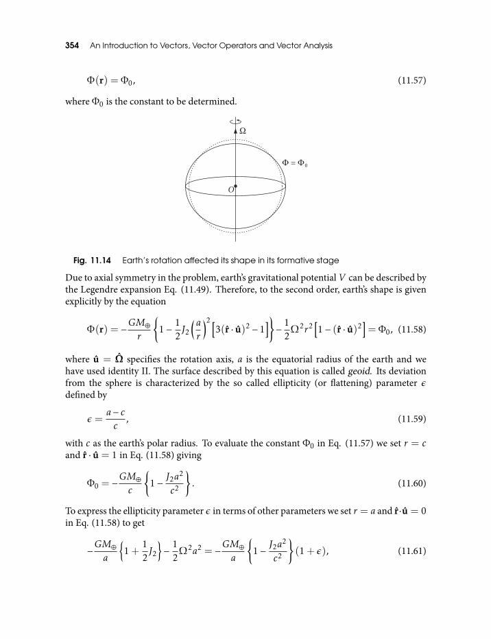
354 An Introduction to Vectors, Vector Operators and Vector Analysis
Φ(r) = Φ0, (11.57)
where Φ0 is the constant to be determined.
Fig. 11.14 Earth’s rotation affected its shape in its formative stage
Due to axial symmetry in the problem, earth’s gravitational potential V can be described bythe Legendre expansion Eq. (11.49). Therefore, to the second order, earth’s shape is givenexplicitly by the equation
Φ(r) = −GM⊕r
1− 1
2J2
(ar
)2 [3(r · u)2 − 1
]− 1
2Ω2r2
[1− (r · u)2
]= Φ0, (11.58)
where u = Ω specifies the rotation axis, a is the equatorial radius of the earth and wehave used identity II. The surface described by this equation is called geoid. Its deviationfrom the sphere is characterized by the so called ellipticity (or flattening) parameter εdefined by
ε =a− cc
, (11.59)
with c as the earth’s polar radius. To evaluate the constant Φ0 in Eq. (11.57) we set r = cand r · u = 1 in Eq. (11.58) giving
Φ0 = −GM⊕c
1− J2a
2
c2
. (11.60)
To express the ellipticity parameter ε in terms of other parameters we set r = a and r·u = 0in Eq. (11.58) to get
−GM⊕a
1+
12J2
− 1
2Ω2a2 = −GM⊕
a
1− J2a
2
c2
(1+ ε), (11.61)
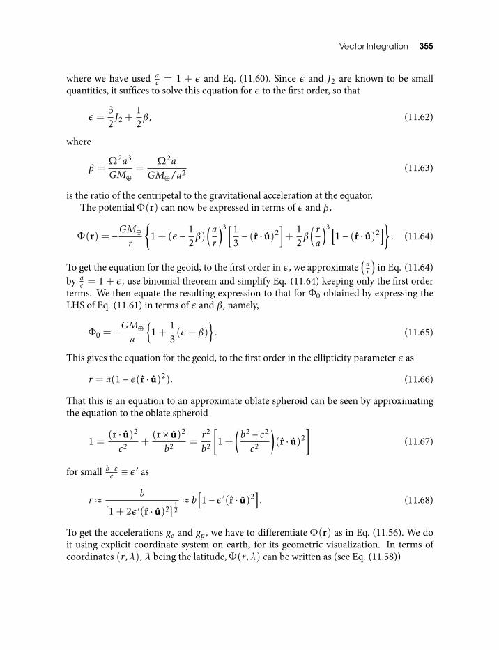
Vector Integration 355
where we have used ac = 1 + ε and Eq. (11.60). Since ε and J2 are known to be small
quantities, it suffices to solve this equation for ε to the first order, so that
ε =32J2 +
12β, (11.62)
where
β =Ω2a3
GM⊕=
Ω2a
GM⊕/a2 (11.63)
is the ratio of the centripetal to the gravitational acceleration at the equator.The potential Φ(r) can now be expressed in terms of ε and β,
Φ(r) = −GM⊕r
1+ (ε − 1
2β)
(ar
)3 [13− (r · u)2
]+
12β( ra
)3 [1− (r · u)2
]. (11.64)
To get the equation for the geoid, to the first order in ε, we approximate(ar
)in Eq. (11.64)
by ac = 1 + ε, use binomial theorem and simplify Eq. (11.64) keeping only the first order
terms. We then equate the resulting expression to that for Φ0 obtained by expressing theLHS of Eq. (11.61) in terms of ε and β, namely,
Φ0 = −GM⊕a
1+
13(ε+ β)
. (11.65)
This gives the equation for the geoid, to the first order in the ellipticity parameter ε as
r = a(1− ε(r · u)2). (11.66)
That this is an equation to an approximate oblate spheroid can be seen by approximatingthe equation to the oblate spheroid
1 =(r · u)2
c2 +(r× u)2
b2 =r2
b2
[1+
(b2 − c2
c2
)(r · u)2
](11.67)
for small b−cc ≡ ε′ as
r ≈ b
[1+ 2ε′(r · u)2]12≈ b
[1− ε′(r · u)2
]. (11.68)
To get the accelerations ge and gp, we have to differentiate Φ(r) as in Eq. (11.56). We doit using explicit coordinate system on earth, for its geometric visualization. In terms ofcoordinates (r,λ), λ being the latitude, Φ(r,λ) can be written as (see Eq. (11.58))
356 An Introduction to Vectors, Vector Operators and Vector Analysis
Φ(r,λ) = −GM⊕r
+GM⊕a
2
2r3 J2(3sin2λ− 1)− 12Ω2r2 cos2λ. (11.69)
and the magnitude of the acceleration g is given by
g = −(∂Φ∂r
)2
+
(1r∂Φ∂λ
)212
. (11.70)
Due to the smallness of ε, g is almost normal to the spherical earth, although it is strictlynormal to the geoid. Thus, g deviates from the radial direction (which defines (λ)) only bya small angle of the order of ε. Therefore,
(∂Φ∂λ
)≈ ε, making the second term in Eq. (11.70)
of the order of ε2 and hence negligible. Therefore,
−g = ∂Φ∂r
=GM⊕r2 − 3
2GM⊕a
2
r4 J2(3sin2λ− 1)−Ω2r(1− sin2λ). (11.71)
From Eq. (11.66) we substitute the value of r on the geoid at arbitrary latitude λ
r = a(1− ε sin2λ
)(11.72)
in Eq. (11.71) and use the binomial expansion(1− ε sin2λ
)−n=
(1+ nε sin2λ · · ·
). (11.73)
Neglecting the products of small quantities and higher orders in ε, we get
−g = GM⊕a2
(1+ 2ε sin2λ
)− 3
2GM⊕a2 J2
(3sin2λ− 1
)−Ω2a
(1− sin2λ
). (11.74)
Putting λ= 0 in Eq. (3.20) we get the value of the equatorial gravity
ge = −GM⊕a2
(1+
32J2 − β
)=GM⊕a2
(1+ ε − 3
2β)
. (11.75)
Similarly, putting λ=π2
in Eq. (2.20) we get the value at the poles
gp =GM⊕a2 (1+ β). (11.76)
Using the given experimental values of ge and gp and the known values of a and Ω we cansolve the simultaneous Eqs (11.75) and (11.76) to get
ε = 0.003376;β = 0.003468 (11.77)
Vector Integration 357
We can substitute these values of ε and β in Eq. (11.62) to get the value of J2 which agreeswith the value of J2 mentioned above, which was obtained using satellite data, within onepercent. This gives us a check on the internal consistency of the theory.
The shape of the earth given by the geoid Eq. (11.66) agrees with measurements ofsea level to within a few meters. However, radar ranging to measure the height of the oceanis accurate to a fraction of a meter. This shows the need to develop more refined modelsfor the shape of the earth. The principal deviation from the geoid is an excessive bulgearound the equator. This is attributed to a retardation of the rotating earth over past millionyears. For a detailed exposition of the physics of the earth, the reader may consult ref [16]and [24].
11.3 Area IntegralWe already know that the magnitude of a vector product like x1 × x2 equals the area ofthe parallelogram with x1 and x2 as its adjacent sides and its direction is that in which aright handed screw advances when rotated in the sense of x1 rotating towards x2. If n isthe unit vector in the direction of x1 × x2 then the area vector representing the area of thecorresponding parallelogram is defined to be
a = ±|x1 × x2|n, (11.78)
where the + sign applies if the rotation of x1 towards x2 is counterclockwise and − signapplies if it is clockwise. This definition of the area vector suggests the followingconstruction of an area integral:
A =12
∫ b
ax× dx =
12
limn→∞
n∑k=1
xk ×∆xk (11.79)
with∑nk=1∆xk = b− a. Note that this is totally a vector relation in which differential area
vectors are added to give the resulting area vector in the limit as |∆x| → 0. If n is largeenough, we can approximate this area integral by the sum
A ≈ 12
n∑k=1
xk ×∆xk
=12
x0 × x1 +12
x1 × x2 + · · ·+12
xn−1 × xn. (11.80)
As depicted in Fig. 11.15, each term in this sum is the area vector of a triangle with onevertex at the origin. The magnitude of the kth term approximates the area swept out bythe line segment represented by the vector variable x as its tip moves continuously alongthe curve joining a and b from xk−1 to xk with its tail at the origin, while the direction ofthe corresponding area vector is consistent with the sense of rotation of x from xk−1 to xk .Thus, the sum in Eq. (11.80) approximates the area vector corresponding to the area swept
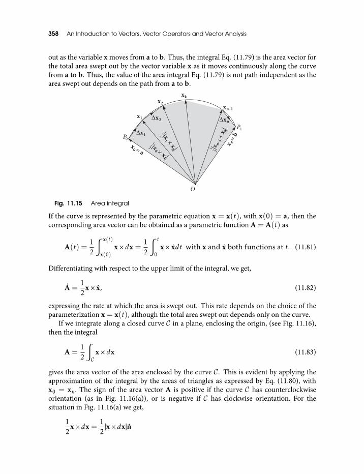
358 An Introduction to Vectors, Vector Operators and Vector Analysis
out as the variable x moves from a to b. Thus, the integral Eq. (11.79) is the area vector forthe total area swept out by the vector variable x as it moves continuously along the curvefrom a to b. Thus, the value of the area integral Eq. (11.79) is not path independent as thearea swept out depends on the path from a to b.
Fig. 11.15 Area integral
If the curve is represented by the parametric equation x = x(t), with x(0) = a, then thecorresponding area vector can be obtained as a parametric function A = A(t) as
A(t) =12
∫ x(t)
x(0)x× dx =
12
∫ t
0x× xdt with x and x both functions at t. (11.81)
Differentiating with respect to the upper limit of the integral, we get,
A =12
x× x, (11.82)
expressing the rate at which the area is swept out. This rate depends on the choice of theparameterization x = x(t), although the total area swept out depends only on the curve.
If we integrate along a closed curve C in a plane, enclosing the origin, (see Fig. 11.16),then the integral
A =12
∫C
x× dx (11.83)
gives the area vector of the area enclosed by the curve C. This is evident by applying theapproximation of the integral by the areas of triangles as expressed by Eq. (11.80), withx0 = xn. The sign of the area vector A is positive if the curve C has counterclockwiseorientation (as in Fig. 11.16(a)), or is negative if C has clockwise orientation. For thesituation in Fig. 11.16(a) we get,
12
x× dx =12|x× dx|n
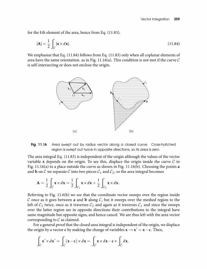
Vector Integration 359
for the kth element of the area, hence from Eq. (11.83),
|A|= 12
∫C|x× dx|. (11.84)
We emphasize that Eq. (11.84) follows from Eq. (11.83) only when all coplanar elements ofarea have the same orientation. as in Fig. 11.16(a). This condition is not met if the curve Cis self-intersecting or does not enclose the origin.
Fig. 11.16 Area swept out by radius vector along a closed curve. Cross-hatchedregion is swept out twice in opposite directions, so its area is zero.
The area integral Eq. (11.83) is independent of the origin although the values of the vectorvariable x depends on the origin. To see this, displace the origin inside the curve C inFig. 11.16(a) to a place outside the curve as shown in Fig. 11.16(b). Choosing the points aand b on C we separate C into two pieces C1 and C2, so the area integral becomes
A =12
∫C
x× dx =12
∫C1
x× dx+12
∫C2
x× dx.
Referring to Fig. 11.6(b) we see that the coordinate vector sweeps over the region insideC once as it goes between a and b along C, but it sweeps over the meshed region to theleft of C2 twice, once as it traverses C2 and again as it traverses C1 and since the sweepsover the latter region are in opposite directions their contributions to the integral havesame magnitude but opposite signs, and hence cancel. We are thus left with the area vectorcorresponding to C as claimed.
For a general proof that the closed area integral is independent of the origin, we displacethe origin by a vector c by making the change of variables x→ x′ = x− c. Then,∫
Cx′ × dx′ =
∫C(x− c)× dx =
∫C
x× dx− c×∫Cdx.
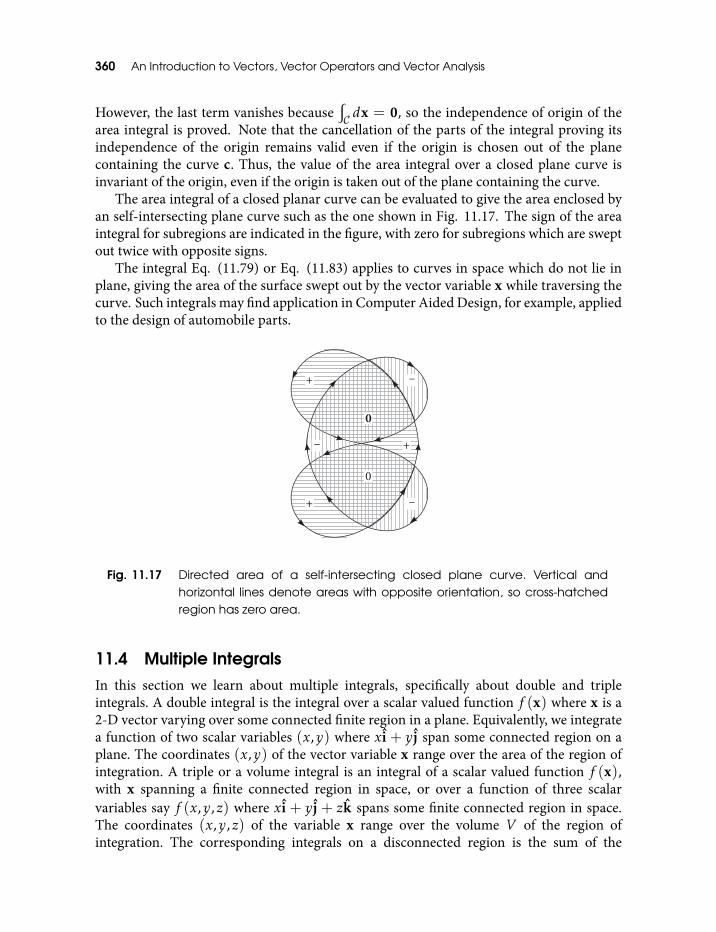
360 An Introduction to Vectors, Vector Operators and Vector Analysis
However, the last term vanishes because∫C dx = 0, so the independence of origin of the
area integral is proved. Note that the cancellation of the parts of the integral proving itsindependence of the origin remains valid even if the origin is chosen out of the planecontaining the curve c. Thus, the value of the area integral over a closed plane curve isinvariant of the origin, even if the origin is taken out of the plane containing the curve.
The area integral of a closed planar curve can be evaluated to give the area enclosed byan self-intersecting plane curve such as the one shown in Fig. 11.17. The sign of the areaintegral for subregions are indicated in the figure, with zero for subregions which are sweptout twice with opposite signs.
The integral Eq. (11.79) or Eq. (11.83) applies to curves in space which do not lie inplane, giving the area of the surface swept out by the vector variable x while traversing thecurve. Such integrals may find application in Computer Aided Design, for example, appliedto the design of automobile parts.
Fig. 11.17 Directed area of a self-intersecting closed plane curve. Vertical andhorizontal lines denote areas with opposite orientation, so cross-hatchedregion has zero area.
11.4 Multiple IntegralsIn this section we learn about multiple integrals, specifically about double and tripleintegrals. A double integral is the integral over a scalar valued function f (x) where x is a2-D vector varying over some connected finite region in a plane. Equivalently, we integratea function of two scalar variables (x,y) where xi + y j span some connected region on aplane. The coordinates (x,y) of the vector variable x range over the area of the region ofintegration. A triple or a volume integral is an integral of a scalar valued function f (x),with x spanning a finite connected region in space, or over a function of three scalarvariables say f (x,y,z) where xi + y j + zk spans some finite connected region in space.The coordinates (x,y,z) of the variable x range over the volume V of the region ofintegration. The corresponding integrals on a disconnected region is the sum of the
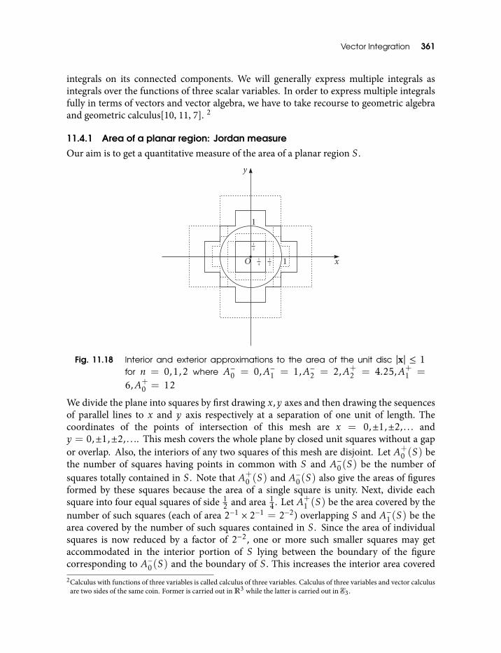
Vector Integration 361
integrals on its connected components. We will generally express multiple integrals asintegrals over the functions of three scalar variables. In order to express multiple integralsfully in terms of vectors and vector algebra, we have to take recourse to geometric algebraand geometric calculus[10, 11, 7]. 2
11.4.1 Area of a planar region: Jordan measure
Our aim is to get a quantitative measure of the area of a planar region S .
Fig. 11.18 Interior and exterior approximations to the area of the unit disc |x| ≤ 1for n = 0,1,2 where A−0 = 0,A−1 = 1,A−2 = 2,A+
2 = 4.25,A+1 =
6,A+0 = 12
We divide the plane into squares by first drawing x,y axes and then drawing the sequencesof parallel lines to x and y axis respectively at a separation of one unit of length. Thecoordinates of the points of intersection of this mesh are x = 0,±1,±2, . . . andy = 0,±1,±2, . . .. This mesh covers the whole plane by closed unit squares without a gapor overlap. Also, the interiors of any two squares of this mesh are disjoint. Let A+
0 (S) bethe number of squares having points in common with S and A−0(S) be the number ofsquares totally contained in S . Note that A+
0 (S) and A−0(S) also give the areas of figuresformed by these squares because the area of a single square is unity. Next, divide eachsquare into four equal squares of side 1
2 and area 14 . Let A+
1 (S) be the area covered by thenumber of such squares (each of area 2−1 × 2−1 = 2−2) overlapping S and A−1(S) be thearea covered by the number of such squares contained in S . Since the area of individualsquares is now reduced by a factor of 2−2, one or more such smaller squares may getaccommodated in the interior portion of S lying between the boundary of the figurecorresponding to A−0(S) and the boundary of S . This increases the interior area covered2Calculus with functions of three variables is called calculus of three variables. Calculus of three variables and vector calculus
are two sides of the same coin. Former is carried out in R3 while the latter is carried out in E3.
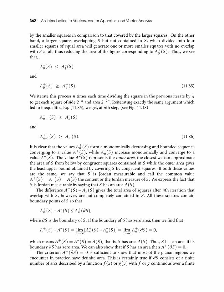
362 An Introduction to Vectors, Vector Operators and Vector Analysis
by the smaller squares in comparison to that covered by the larger squares. On the otherhand, a larger square, overlapping S but not contained in S, when divided into foursmaller squares of equal area will generate one or more smaller squares with no overlapwith S at all, thus reducing the area of the figure corresponding to A+
0 (S). Thus, we seethat,
A−0(S) ≤ A−1(S)
and
A+0 (S) ≥ A+
1 (S). (11.85)
We iterate this process n times each time dividing the square in the previous iterate by 12
to get each square of side 2−n and area 2−2n. Reiterating exactly the same argument whichled to inequalities Eq. (11.85), we get, at nth step, (see Fig. 11.18)
A−n−1(S) ≤ A−n(S)
and
A+n−1(S) ≥ A+
n (S). (11.86)
It is clear that the values A+n (S) form a monotonically decreasing and bounded sequence
converging to a value A+(S), while A−n(S) increase monotonically and converge to avalue A−(S). The value A−(S) represents the inner area, the closest we can approximatethe area of S from below by congruent squares contained in S while the outer area givesthe least upper bound obtained by covering S by congruent squares. If both these valuesare the same, we say that S is Jordan measurable and call the common valueA+(S) = A−(S) = A(S) the content or the Jordan measure of S . We express the fact thatS is Jordan measurable by saying that S has an area A(S).
The difference A+n (S) − A−n(S) gives the total area of squares after nth iteration that
overlap with S, however, are not completely contained in S . All these squares containboundary points of S so that
A+n (S)−A−n(S) ≤ A+
n (∂S),
where ∂S is the boundary of S . If the boundary of S has zero area, then we find that
A+(S)−A−(S) = limn→∞
[A+n (S)−A−n(S)] = lim
n→∞A+n (∂S) = 0,
which means A+(S) = A−(S) = A(S), that is, S has area A(S). Thus, S has an area if itsboundary ∂S has zero area. We can also show that if S has an area then A+(∂S) = 0.
The criterion A+(∂S) = 0 is sufficient to show that most of the planar regions weencounter in practice have definite area. This is certainly true if ∂S consists of a finitenumber of arcs described by a function f (x) or g(y) with f or g continuous over a finite
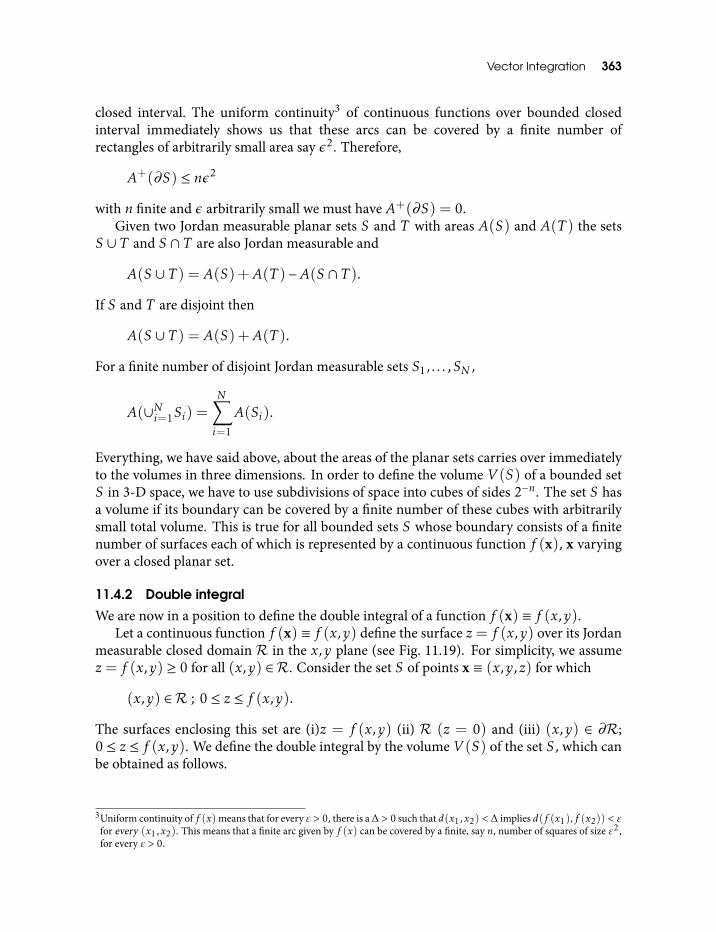
Vector Integration 363
closed interval. The uniform continuity3 of continuous functions over bounded closedinterval immediately shows us that these arcs can be covered by a finite number ofrectangles of arbitrarily small area say ε2. Therefore,
A+(∂S) ≤ nε2
with n finite and ε arbitrarily small we must have A+(∂S) = 0.Given two Jordan measurable planar sets S and T with areas A(S) and A(T ) the sets
S ∪ T and S ∩ T are also Jordan measurable and
A(S ∪ T ) = A(S) +A(T )−A(S ∩ T ).
If S and T are disjoint then
A(S ∪ T ) = A(S) +A(T ).
For a finite number of disjoint Jordan measurable sets S1, . . . ,SN ,
A(∪Ni=1Si) =N∑i=1
A(Si).
Everything, we have said above, about the areas of the planar sets carries over immediatelyto the volumes in three dimensions. In order to define the volume V (S) of a bounded setS in 3-D space, we have to use subdivisions of space into cubes of sides 2−n. The set S hasa volume if its boundary can be covered by a finite number of these cubes with arbitrarilysmall total volume. This is true for all bounded sets S whose boundary consists of a finitenumber of surfaces each of which is represented by a continuous function f (x), x varyingover a closed planar set.
11.4.2 Double integral
We are now in a position to define the double integral of a function f (x) ≡ f (x,y).Let a continuous function f (x) ≡ f (x,y) define the surface z = f (x,y) over its Jordan
measurable closed domain R in the x,y plane (see Fig. 11.19). For simplicity, we assumez = f (x,y) ≥ 0 for all (x,y) ∈ R. Consider the set S of points x ≡ (x,y,z) for which
(x,y) ∈ R ; 0 ≤ z ≤ f (x,y).
The surfaces enclosing this set are (i)z = f (x,y) (ii) R (z = 0) and (iii) (x,y) ∈ ∂R;0 ≤ z ≤ f (x,y). We define the double integral by the volume V (S) of the set S, which canbe obtained as follows.
3Uniform continuity of f (x) means that for every ε > 0, there is a ∆ > 0 such that d(x1,x2) < ∆ implies d(f (x1),f (x2)) < εfor every (x1,x2). This means that a finite arc given by f (x) can be covered by a finite, say n, number of squares of size ε2,for every ε > 0.
364 An Introduction to Vectors, Vector Operators and Vector Analysis
Fig. 11.19 Evaluation of a double integral
We divideR into non-overlapping Jordan measurable closed setsR1, . . . ,RN . Let hi be theminimum and Hi be the maximum of f (x,y) with (x,y) ∈ Ri . The cylinder with heighthi and baseRi has the volume hiA(Ri) whereA(Ri) is the area ofRi . These cylinders donot overlap. Similarly, the cylinders with height Hi and base Ri do not overlap and havethe volumeHiA(Ri). It follows that
N∑i=1
hiA(Ri) ≤ V (S) ≤N∑i=1
HiA(Ri). (11.87)
The sums in this inequality are respectively called the lower sum and the upper sum.We now make the subdivision of R finer and finer, such that the number of subsets thenumber of subdivisions and the largest diameter of Ri ; i = 1, . . . ,N tends to zero. Thecontinuous function f (x,y) is uniformly continuous in the closed and bounded set R, sothat the maximum difference Hi − hi tends to zero with the maximum diameter over thesets Ri of the subdivision. The differences over the upper and the lower sum also tend tozero, since,
N∑i=1
HiA (Ri)−N∑i=1
hiA (Ri) =N∑i=1
(Hi − hi)A (Ri)
≤[maxi
(Hi − hi)] N∑k=1
A (Rk)
=[maxi
(Hi − hi)]A(R). (11.88)
It follows from inequality Eq. (11.87) that the upper and lower sum both converge to thelimit V (S) as the number of subdivisions N → ∞ or the largest diameter tends to zero.
Vector Integration 365
We obtain the same limiting value if we take the value of the function f (xi ,yi) at a point(xi ,yi) ∈ Ri , instead of hi or Hi . We call the limit V (S) the double integral of f over thesetR and write
V (S) =
∫ ∫Rf (x,y)dR. (11.89)
Suppose, we now lift the restriction z = f (x,y) > 0. Due to continuity of f (x,y) thesurface (x,y) ∈ R ; z = f (x,y) may cut the x,y plane in some continuous curve and theset S defined above is divided into two (or more, but we assume two) sets, one above andthe other below the x,y plane, each corresponding to two distinct parts,R+ andR− of thedomainR. These are the set S+ given by (x,y) ∈ R ; z = f (x,y) > 0 and the set S− givenby (x,y) ∈ R ; z = f (x,y) < 0. We define a new set S∓ by (x,y) ∈ R ; z = −f (x,y) > 0.Both these are the sets of points above the x,y plane so that∫ ∫
R+f (x,y)dR= V (S+) and
∫ ∫R−
(−f(x,y))dR= V(S∓) = V(S−).
This means∫ ∫Rf (x,y)dR= V (S+)−V (S−).
We can summarize as follows. Consider a closed and bounded setRwith areaA(R) = ∆Rand a function f (x,y) that is continuous everywhere in R including its boundary. WesubdivideR intoN non-overlapping Jordan measurable subsetsR1,R2, . . . ,RN with areas∆R1,∆R2, . . . ,∆RN . InRi we choose an arbitrary point (xi ,yi) where f (xi ,yi) = fi andform the sum
VN =N∑i=1
fiA(Ri).
Then, we have the theorem:If the number N tends to infinity and simultaneously the greatest of the diameters of
the subregions tends to zero, then VN tends to a limit V . This limit is independent of theparticular nature of the subdivision of R and of the choice of the point (xi ,yi) in Ri . Wecall the limit V the double integral of the function f (x,y) over the region R and denoteit by ∫ ∫
Rf (x,y)dR.
Since A(∂R) = 0 we can choose allRi to lie entirely in the interior ofR having no pointscommon with the boundary ofR.
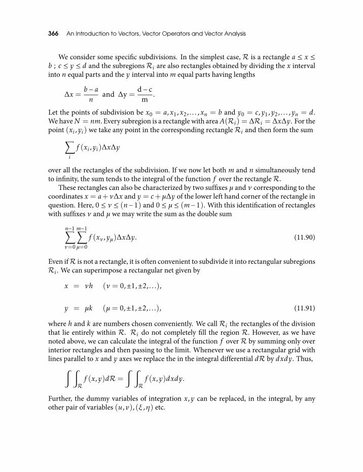
366 An Introduction to Vectors, Vector Operators and Vector Analysis
We consider some specific subdivisions. In the simplest case, R is a rectangle a ≤ x ≤b ; c ≤ y ≤ d and the subregionsRi are also rectangles obtained by dividing the x intervalinto n equal parts and the y interval intom equal parts having lengths
∆x =b − an
and ∆y =d− c
m.
Let the points of subdivision be x0 = a,x1,x2, . . . ,xn = b and y0 = c,y1,y2, . . . ,yn = d.We haveN = nm. Every subregion is a rectangle with areaA(Ri) = ∆Ri = ∆x∆y. For thepoint (xi ,yi) we take any point in the corresponding rectangleRi and then form the sum∑
i
f (xi ,yi)∆x∆y
over all the rectangles of the subdivision. If we now let both m and n simultaneously tendto infinity, the sum tends to the integral of the function f over the rectangleR.
These rectangles can also be characterized by two suffixes µ and ν corresponding to thecoordinates x = a+ν∆x and y = c+µ∆y of the lower left hand corner of the rectangle inquestion. Here, 0 ≤ ν ≤ (n−1) and 0 ≤ µ ≤ (m−1). With this identification of rectangleswith suffixes ν and µ we may write the sum as the double sum
n−1∑ν=0
m−1∑µ=0
f (xν ,yµ)∆x∆y. (11.90)
Even ifR is not a rectangle, it is often convenient to subdivide it into rectangular subregionsRi . We can superimpose a rectangular net given by
x = νh (ν = 0,±1,±2, . . .),
y = µk (µ= 0,±1,±2, . . .), (11.91)
where h and k are numbers chosen conveniently. We callRi the rectangles of the divisionthat lie entirely within R. Ri do not completely fill the region R. However, as we havenoted above, we can calculate the integral of the function f overR by summing only overinterior rectangles and then passing to the limit. Whenever we use a rectangular grid withlines parallel to x and y axes we replace the in the integral differential dR by dxdy. Thus,∫ ∫
Rf (x,y)dR=
∫ ∫Rf (x,y)dxdy.
Further, the dummy variables of integration x,y can be replaced, in the integral, by anyother pair of variables (u,v), (ξ,η) etc.
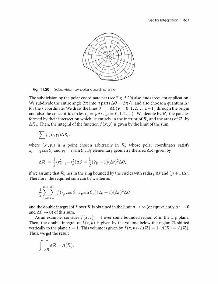
Vector Integration 367
Fig. 11.20 Subdivision by polar coordinate net
The subdivision by the polar coordinate net (see Fig. 3.20) also finds frequent application.We subdivide the entire angle 2π into n parts ∆θ = 2π/n and also choose a quantum ∆rfor the r coordinate. We draw the lines θ = ν∆θ(ν = 0, 1,2, . . . ,n−1) through the originand also the concentric circles rµ = µ∆r, (µ = 0,1,2, . . .). We denote by Ri the patchesformed by their intersection which lie entirely in the interior of R, and the areas of Ri by∆Ri . Then, the integral of the function f (x,y) is given by the limit of the sum∑
f (xi ,yi)∆Ri ,
where (xi ,yi) is a point chosen arbitrarily in Ri whose polar coordinates satisfyxi = ri cosθi and yi = ri sinθi . By elementary geometry the area ∆Ri given by
∆Ri =12(r2µ+1 − r
2µ)∆θ =
12(2µ+ 1)(∆r)2∆θ,
if we assume thatRi lies in the ring bounded by the circles with radia µ∆r and (µ+1)∆r .Therefore, the required sum can be written as
12
n−1∑µ=0
n−1∑ν=0
f (rµ cosθν ,rµ sinθν)(2µ+ 1)(∆r)2∆θ
and the double integral of f overR is obtained in the limit n→∞ (or equivalently ∆r→ 0and ∆θ→ 0) of this sum.
As an example, consider f (x,y) = 1 over some bounded region R in the x,y plane.Then, the double integral of f (x,y) is given by the volume below the region R shiftedvertically to the plane z = 1. This volume is given by f (x,y) ·A(R) = 1 ·A(R) = A(R).Thus, we get the result∫ ∫
RdR= A(R).
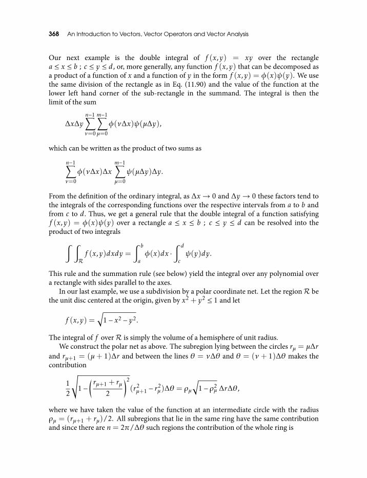
368 An Introduction to Vectors, Vector Operators and Vector Analysis
Our next example is the double integral of f (x,y) = xy over the rectanglea ≤ x ≤ b ; c ≤ y ≤ d, or, more generally, any function f (x,y) that can be decomposed asa product of a function of x and a function of y in the form f (x,y) = φ(x)ψ(y). We usethe same division of the rectangle as in Eq. (11.90) and the value of the function at thelower left hand corner of the sub-rectangle in the summand. The integral is then thelimit of the sum
∆x∆yn−1∑ν=0
m−1∑µ=0
φ(ν∆x)ψ(µ∆y),
which can be written as the product of two sums as
n−1∑ν=0
φ(ν∆x)∆xm−1∑µ=0
ψ(µ∆y)∆y.
From the definition of the ordinary integral, as ∆x→ 0 and ∆y → 0 these factors tend tothe integrals of the corresponding functions over the respective intervals from a to b andfrom c to d. Thus, we get a general rule that the double integral of a function satisfyingf (x,y) = φ(x)ψ(y) over a rectangle a ≤ x ≤ b ; c ≤ y ≤ d can be resolved into theproduct of two integrals∫ ∫
Rf (x,y)dxdy =
∫ b
aφ(x)dx ·
∫ d
cψ(y)dy.
This rule and the summation rule (see below) yield the integral over any polynomial overa rectangle with sides parallel to the axes.
In our last example, we use a subdivision by a polar coordinate net. Let the regionR bethe unit disc centered at the origin, given by x2 + y2 ≤ 1 and let
f (x,y) =√
1− x2 − y2.
The integral of f overR is simply the volume of a hemisphere of unit radius.We construct the polar net as above. The subregion lying between the circles rµ = µ∆r
and rµ+1 = (µ+ 1)∆r and between the lines θ = ν∆θ and θ = (ν + 1)∆θ makes thecontribution
12
√1−
(rµ+1 + rµ
2
)2
(r2µ+1 − r
2µ)∆θ = ρµ
√1− ρ2
µ ∆r∆θ,
where we have taken the value of the function at an intermediate circle with the radiusρµ = (rµ+1 + rµ)/2. All subregions that lie in the same ring have the same contributionand since there are n= 2π/∆θ such regions the contribution of the whole ring is
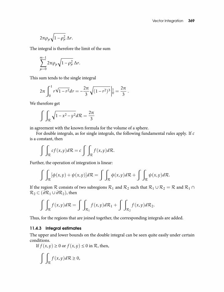
Vector Integration 369
2πρµ√
1− ρ2µ ∆r.
The integral is therefore the limit of the sum
m−1∑µ=0
2πρµ√
1− ρ2µ ∆r.
This sum tends to the single integral
2π∫ 1
0r√
1− r2dr = −2π3
√(1− r2)3
∣∣∣∣∣10 = 2π3
.
We therefore get∫ ∫R
√1− x2 − y2dR=
2π3
in agreement with the known formula for the volume of a sphere.For double integrals, as for single integrals, the following fundamental rules apply. If c
is a constant, then∫ ∫Rcf (x,y)dR= c
∫ ∫Rf (x,y)dR.
Further, the operation of integration is linear:∫ ∫R[φ(x,y) +ψ(x,y)]dR=
∫ ∫Rφ(x,y)dR+
∫ ∫Rψ(x,y)dR.
If the region R consists of two subregions R1 and R2 such that R1 ∪R2 = R and R1 ∩R2 ⊂ (∂R1 ∪∂R2), then∫ ∫
Rf (x,y)dR=
∫ ∫R1
f (x,y)dR1 +
∫ ∫R2
f (x,y)dR2.
Thus, for the regions that are joined together, the corresponding integrals are added.
11.4.3 Integral estimates
The upper and lower bounds on the double integral can be seen quite easily under certainconditions.
If f (x,y) ≥ 0 or f (x,y) ≤ 0 inR, then,∫ ∫Rf (x,y)dR≥ 0,
370 An Introduction to Vectors, Vector Operators and Vector Analysis
or, ∫ ∫Rf (x,y)dR≤ 0.
From this we see that, if the inequality
f (x,y) ≥ g(x,y)
holds everywhere inR, then,∫ ∫Rf (x,y)dR≥
∫ ∫Rg(x,y)dR.
From this it follows that∫ ∫Rf (x,y)dR≤
∫ ∫R|f (x,y)|dR
and ∫ ∫Rf (x,y)dR≥ −
∫ ∫R|f (x,y)|dR.
These two inequalities can be combined:∣∣∣∣∣∫ ∫Rf (x,y)dR
∣∣∣∣∣ ≤ ∫ ∫R|f (x,y)|dR.
If m is the greatest lower bound and M is the least upper bound of the function f (x,y) inR, and ∆R is the area ofR, then,
m∆R≤∫ ∫
Rf (x,y)dR≤M∆R.
The integral can then be expressed as∫ ∫Rf (x,y)dR= µ∆R
with µ lying between m and M . The precise value of µ cannot be specified more exactly.This equation is called the mean value theorem in integral calculus. Generalizing, we cansay that for an arbitrary positive continuous function p(x,y) onR,∫ ∫
Rp(x,y)f (x,y)dR= µ
∫ ∫Rp(x,y)dR,
Vector Integration 371
where µ is a number between the greatest and the lowest values of f (x,y) onR that cannotbe further specified.
We close by making the following two observations. The first is that a double integral onR varies continuously with the function to be integrated. This means, given two functionsf and g satisfying
|f (x,y)− g(x,y)| < ε, (x,y) ∈ R,
where ε > 0 is a fixed number, then the integrals∫ ∫R f (x,y)dR and
∫ ∫R g(x,y)dR differ
by less than ε∆Rwhere ∆R is the area ofR, that is, by less than a number that goes to zerowith ε. Similarly, we see that the integral of a function varies continuously with the region.Suppose that the regionR2 is obtained fromR1 by removing portions whose total area isless than ε > 0 and f (x,y) be a function continuous on both regions with |f (x,y)| < Mwhere M is a fixed number. The two integrals
∫ ∫R1f (x,y)dR and
∫ ∫R2f (x,y)dR then
differ by less than Mε, that is, by a number less than that tends to zero with ε. Both theseobservations follow from the fundamental rules stated above.
Thus, we see that an integral over a region R can be approximated as closely as weplease by evaluating it over a subregion of R whose total area differs from the area of Rby a sufficiently small amount. In a regionR we can construct a polygon whose total areadiffers from that of R by as little an amount as we please. In particular, we can constructthis polygon by piecing together rectangles whose sides are lines parallel to the axes.
11.4.4 Triple integrals
Whatever we have said about the integrals over a bounded, closed and connected region inthe x,y plane gets carried over, without further complication or introduction of new ideas,to the integrals over a bounded, closed and connected region in the 3-D space called tripleintegrals. In order to treat the integral over a 3-D region R, we need to subdivide R intoclosed non-overlapping Jordan measurable subregionsR1,R2, . . . ,RN that completely fillR. If f (x) ≡ f (x,y,z) is a function that is continuous in the regionR and if (xi ,yi ,zi) isan arbitrary point in the regionRi , we again form the sum
N∑i=1
f (xi ,yi ,zi)∆Ri ,
where ∆Ri is now the volume of the regionRi . The sum may be taken over all regionsRi ,or, over thoseRi which are interior toR. If we now take the limit asN →∞ such that thelargest of the diameters ofRi tends to zero, then the sum tends to a limiting value which isindependent of the mode of subdivision or the choice of the intermediate points. We callthis limit the integral of the function f (x,y,z) over the regionR and write it as∫ ∫
Rf (x,y,z)dR.
372 An Introduction to Vectors, Vector Operators and Vector Analysis
In particular, if the we subdivide into rectangular boxes with sides ∆x,∆y,∆z then thevolumes of all the inner regions Ri have the same value ∆x∆y∆z and the correspondingintegral is written as∫ ∫ ∫
Rf (x,y,z)dxdydz.
Apart from the changes in notation all that has been said about the double integral is validfor the triple integral.
11.4.5 Multiple integrals as successive single integrals
Evaluation of multiple integrals can be reduced to successive evaluation of single integrals.This allows us to employ all the standard techniques available to evaluate indefiniteintegrals of a function of a single variable.
Integrals over a rectangleWe first consider the case where the region of integration R is a rectangle a ≤ x ≤ b, c ≤y ≤ d. We want to integrate a continuous function f (x,y) over R. The procedure to dothis is given in the following theorem, which we state without proof.
To find∫ ∫R f (x,y)dxdy we first regard y as constant and integrate f (x,y) with respect
to x between the limits a and b. The resulting integral,
φ(y) =
∫ b
af (x,y)dx
is a function of y, which we integrate between the limits c and d to obtain the doubleintegral. In symbols,∫ ∫
Rf (x,y)dxdy =
∫ d
cφ(y)dy, φ(y) =
∫ b
af (x,y)dx,
or, ∫ ∫Rf (x,y)dxdy =
∫ d
cdy
∫ b
af (x,y)dx. (11.92)
Since the roles of x and y are interchangeable, we have∫ ∫Rf (x,y)dxdy =
∫ b
adx
∫ d
cf (x,y)dy. (11.93)
Equations (11.92) and (11.93) together imply∫ d
cdy
∫ b
af (x,y)dx =
∫ b
adx
∫ d
cf (x,y)dy. (11.94)
Vector Integration 373
That is, in the repeated integration of a continuous function with constant limits ofintegration, the order of integration can be reversed. This facility of changing the order ofintegration is particularly useful in the explicit calculation of simple definite integrals forwhich no indefinite integral can be found.
Exercise Evaluate I =∫ ∞
0
e−ax − e−bx
xdx.
Solution We can write
I = limT→∞
∫ T
0dx
∫ b
ae−xydy,
from which we obtain by changing the order of integration
I = limT→∞
∫ b
a
1− e−T y
ydy = log
ba− limT→∞
∫ b
a
e−T y
ydy.
By virtue of the relation∫ b
a
e−T y
ydy =
∫ T b
T a
e−y
ydy,
the second integral tends to zero as T increases, so that,
I =
∫ ∞0
e−ax − e−bx
xdx = log
ba
.
Exercise If f (t) is a C1 function of t except at countably many points for t ≥ 0 and if theintegral∫ ∞
1
f (t)
tdt
exists, then show that, for positive a and b,
I =
∫ ∞0
f (ax)− f (bx)x
dx = f (0) logba
.
Hint Write
I =
∫ ∞0dx
∫ a
bf ′(xy)dy
and change the order of integration.
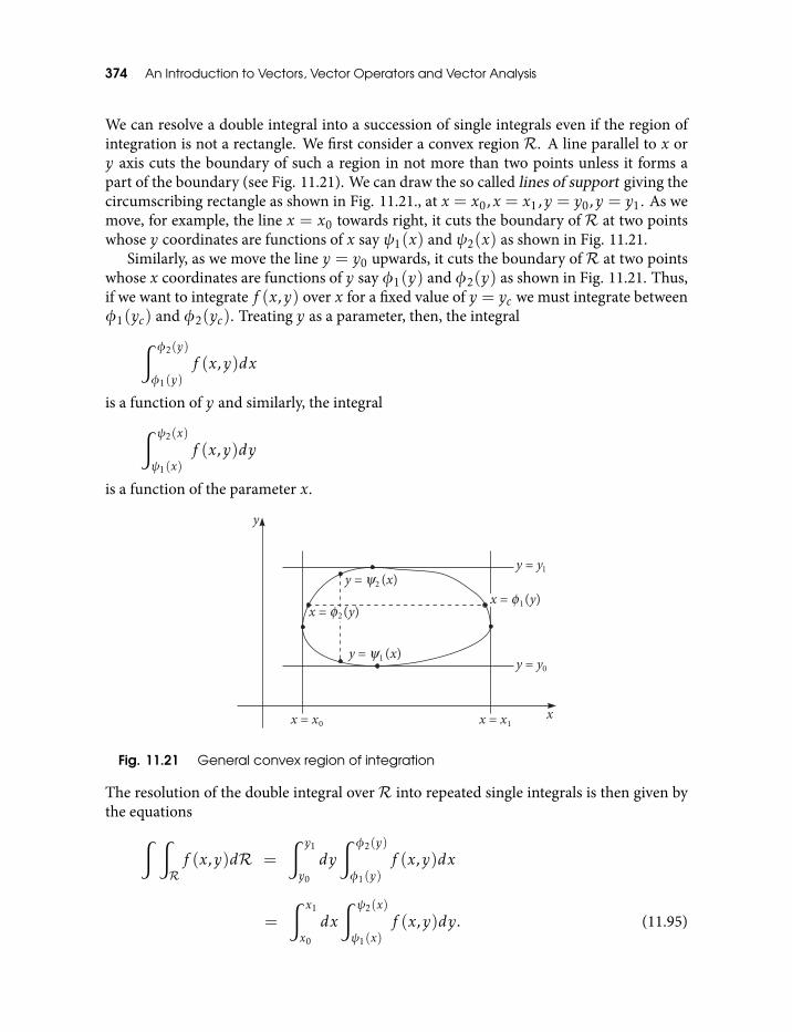
374 An Introduction to Vectors, Vector Operators and Vector Analysis
We can resolve a double integral into a succession of single integrals even if the region ofintegration is not a rectangle. We first consider a convex region R. A line parallel to x ory axis cuts the boundary of such a region in not more than two points unless it forms apart of the boundary (see Fig. 11.21). We can draw the so called lines of support giving thecircumscribing rectangle as shown in Fig. 11.21., at x = x0,x = x1,y = y0,y = y1. As wemove, for example, the line x = x0 towards right, it cuts the boundary of R at two pointswhose y coordinates are functions of x say ψ1(x) and ψ2(x) as shown in Fig. 11.21.
Similarly, as we move the line y = y0 upwards, it cuts the boundary ofR at two pointswhose x coordinates are functions of y say φ1(y) and φ2(y) as shown in Fig. 11.21. Thus,if we want to integrate f (x,y) over x for a fixed value of y = yc we must integrate betweenφ1(yc) and φ2(yc). Treating y as a parameter, then, the integral∫ φ2(y)
φ1(y)f (x,y)dx
is a function of y and similarly, the integral∫ ψ2(x)
ψ1(x)f (x,y)dy
is a function of the parameter x.
Fig. 11.21 General convex region of integration
The resolution of the double integral overR into repeated single integrals is then given bythe equations∫ ∫
Rf (x,y)dR =
∫ y1
y0
dy
∫ φ2(y)
φ1(y)f (x,y)dx
=
∫ x1
x0
dx
∫ ψ2(x)
ψ1(x)f (x,y)dy. (11.95)
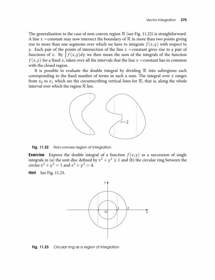
Vector Integration 375
The generalization to the case of non-convex region R (see Fig. 11.22) is straightforward.A line x =constant may now intersect the boundary of R in more than two points givingrise to more than one segments over which we have to integrate f (x,y) with respect toy. Each pair of the points of intersection of the line x =constant gives rise to a pair offunctions of x. By
∫f (x,y)dy we then mean the sum of the integrals of the function
f (x,y) for a fixed x, taken over all the intervals that the line x =constant has in commonwith the closed region.
It is possible to evaluate the double integral by dividing R into subregions eachcorresponding to the fixed number of terms in such a sum. The integral over x rangesfrom x0 to x1 which are the circumscribing vertical lines for R, that is, along the wholeinterval over which the regionR lies.
Fig. 11.22 Non-convex region of integration
Exercise Express the double integral of a function f (x,y) as a succession of singleintegrals in (a) the unit disc defined by x2 + y2 ≤ 1 and (b) the circular ring between thecircles x2 + y2 = 1 and x2 + y2 = 4.
Hint See Fig. 11.23.
Fig. 11.23 Circular ring as a region of integration
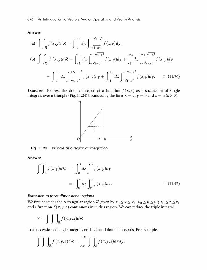
376 An Introduction to Vectors, Vector Operators and Vector Analysis
Answer
(a)∫ ∫
Rf (x,y)dR=
∫ +1
−1dx
∫ +√
1−x2
−√
1−x2f (x,y)dy.
(b)∫ ∫
Rf (x,y)dR=
∫ −1
−2dx
∫ +√
4−x2
−√
4−x2f (x,y)dy+
∫ 2
1dx
∫ +√
4−x2
−√
4−x2f (x,y)dy
+
∫ +1
−1dx
∫ +√
1−x2
−√
4−x2f (x,y)dy+
∫ +1
−1dx
∫ +√
4−x2
−√
1−x2f (x,y)dy. (11.96)
Exercise Express the double integral of a function f (x,y) as a succession of singleintegrals over a triangle (Fig. 11.24) bounded by the lines x = y, y = 0 and x = a (a > 0).
Fig. 11.24 Triangle as a region of integration
Answer∫ ∫Rf (x,y)dR =
∫ a
0dx
∫ x
0f (x,y)dy
=
∫ a
0dy
∫ a
yf (x,y)dx. (11.97)
Extension to three dimensional regionsWe first consider the rectangular regionR given by x0 ≤ x ≤ x1; y0 ≤ y ≤ y1; z0 ≤ z ≤ z1and a function f (x,y,z) continuous in in this region. We can reduce the triple integral
V =
∫ ∫ ∫Rf (x,y,z)dR
to a succession of single integrals or single and double integrals. For example,∫ ∫ ∫Rf (x,y,z)dR=
∫ z1
z0
∫ ∫Bf (x,y,z)dxdy,
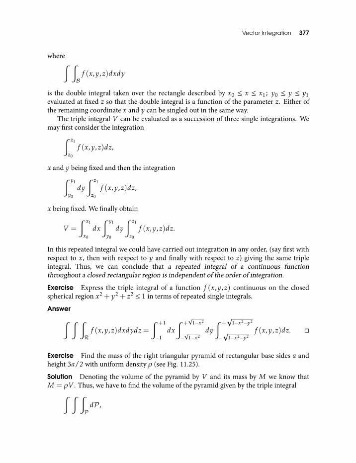
Vector Integration 377
where∫ ∫Bf (x,y,z)dxdy
is the double integral taken over the rectangle described by x0 ≤ x ≤ x1; y0 ≤ y ≤ y1evaluated at fixed z so that the double integral is a function of the parameter z. Either ofthe remaining coordinate x and y can be singled out in the same way.
The triple integral V can be evaluated as a succession of three single integrations. Wemay first consider the integration∫ z1
z0
f (x,y,z)dz,
x and y being fixed and then the integration∫ y1
y0
dy
∫ z1
z0
f (x,y,z)dz,
x being fixed. We finally obtain
V =
∫ x1
x0
dx
∫ y1
y0
dy
∫ z1
z0
f (x,y,z)dz.
In this repeated integral we could have carried out integration in any order, (say first withrespect to x, then with respect to y and finally with respect to z) giving the same tripleintegral. Thus, we can conclude that a repeated integral of a continuous functionthroughout a closed rectangular region is independent of the order of integration.
Exercise Express the triple integral of a function f (x,y,z) continuous on the closedspherical region x2 + y2 + z2 ≤ 1 in terms of repeated single integrals.
Answer∫ ∫ ∫Rf (x,y,z)dxdydz =
∫ +1
−1dx
∫ +√
1−x2
−√
1−x2dy
∫ +√
1−x2−y2
−√
1−x2−y2f (x,y,z)dz.
Exercise Find the mass of the right triangular pyramid of rectangular base sides a andheight 3a/2 with uniform density ρ (see Fig. 11.25).
Solution Denoting the volume of the pyramid by V and its mass by M we know thatM = ρV . Thus, we have to find the volume of the pyramid given by the triple integral∫ ∫ ∫
PdP ,
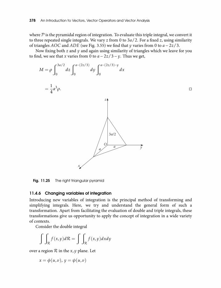
378 An Introduction to Vectors, Vector Operators and Vector Analysis
where P is the pyramidal region of integration. To evaluate this triple integral, we convert itto three repeated single integrals. We vary z from 0 to 3a/2. For a fixed z, using similarityof triangles AOC and ADE (see Fig. 3.55) we find that y varies from 0 to a− 2z/3.
Now fixing both z and y and again using similarity of triangles which we leave for youto find, we see that x varies from 0 to a− 2z/3− y. Thus we get,
M = ρ
∫ 3a/2
0dz
∫ a−(2z/3)
0dy
∫ a−(2z/3)−y
0dx
=14a3ρ.
Fig. 11.25 The right triangular pyramid
11.4.6 Changing variables of integration
Introducing new variables of integration is the principal method of transforming andsimplifying integrals. Here, we try and understand the general form of such atransformation. Apart from facilitating the evaluation of double and triple integrals, thesetransformations give us opportunity to apply the concept of integration in a wide varietyof contexts.
Consider the double integral∫ ∫Rf (x,y)dR=
∫ ∫Rf (x,y)dxdy
over a regionR in the x,y plane. Let
x = φ(u,v), y = ψ(u,v)
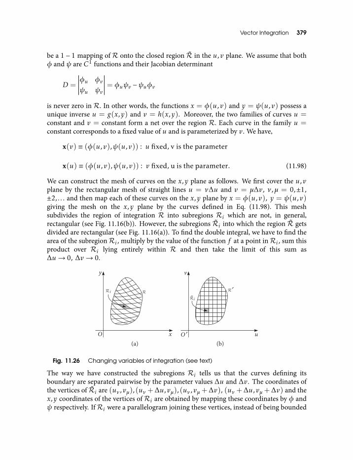
Vector Integration 379
be a 1− 1 mapping of R onto the closed region R in the u,v plane. We assume that bothφ and ψ are C1 functions and their Jacobian determinant
D =
∣∣∣∣∣∣φu φvψu ψv
∣∣∣∣∣∣= φuψv −ψuφv
is never zero in R. In other words, the functions x = φ(u,v) and y = ψ(u,v) possess aunique inverse u = g(x,y) and v = h(x,y). Moreover, the two families of curves u =constant and v = constant form a net over the region R. Each curve in the family u =constant corresponds to a fixed value of u and is parameterized by v. We have,
x(v) ≡ (φ(u,v),ψ(u,v)) : u fixed, v is the parameter
x(u) ≡ (φ(u,v),ψ(u,v)) : v fixed, u is the parameter. (11.98)
We can construct the mesh of curves on the x,y plane as follows. We first cover the u,vplane by the rectangular mesh of straight lines u = ν∆u and v = µ∆v, ν,µ = 0,±1,±2, . . . and then map each of these curves on the x,y plane by x = φ(u,v), y = ψ(u,v)giving the mesh on the x,y plane by the curves defined in Eq. (11.98). This meshsubdivides the region of integration R into subregions Ri which are not, in general,rectangular (see Fig. 11.16(b)). However, the subregions Ri into which the region R getsdivided are rectangular (see Fig. 11.16(a)). To find the double integral, we have to find thearea of the subregionRi , multiply by the value of the function f at a point inRi , sum thisproduct over Ri lying entirely within R and then take the limit of this sum as∆u→ 0, ∆v→ 0.
Fig. 11.26 Changing variables of integration (see text)
The way we have constructed the subregions Ri tells us that the curves defining itsboundary are separated pairwise by the parameter values ∆u and ∆v. The coordinates ofthe vertices of Ri are (uν ,vµ), (uν +∆u,vµ), (uν ,vµ+∆v), (uν +∆u,vµ+∆v) and thex,y coordinates of the vertices ofRi are obtained by mapping these coordinates by φ andψ respectively. IfRi were a parallelogram joining these vertices, instead of being bounded
380 An Introduction to Vectors, Vector Operators and Vector Analysis
by curves, then the area of Ri is given by the absolute value of the determinant (or theabsolute value of the cross product of the corresponding vectors)∣∣∣∣∣∣φ(uν +∆u,vµ)−φ(uν ,vµ) φ(uν ,vµ+∆v)−φ(uν ,vµ)
ψ(uν +∆u,vµ)−ψ(uν ,vµ) ψ(uν ,vµ+∆v)−ψ(uν ,vµ)
∣∣∣∣∣∣ ·Since φ and ψ are C1, we can approximate, for example, φ(uν +∆u,vµ) −φ(uν ,vµ) byφu(uν ,vµ)∆u∆v so that the area ofRi is approximated by the absolute value of∣∣∣∣∣∣φu(uν ,vµ) φv(uν ,vµ)
ψu(uν ,vµ) ψv(uν ,vµ)
∣∣∣∣∣∣∆u∆v = ∆u∆vD.
Thus, forming the required sum and passing to the limit as ∆u → 0, ∆v → 0, we obtainthe expression for the double integral transformed to the new variables,∫ ∫
Rf (φ(u,v),ψ(u,v))|D |dudv.
We will not pause here to show that the area of Ri coincides with the correspondingparallelogram in limit ∆u→ 0, ∆v→ 0 and state the final result:
If the transformation x = φ(u,v);y = ψ(u,v) represents a continuous 1− 1 mappingof the closed Jordan measurable region R of the x,y plane to a region R of the u,v planeand if the functions φ and ψ are C1 and their Jacobian
d(x,y)d(u,v)
= φuψv −ψuφv
is everywhere different from zero, then∫ ∫Rf (x,y)dxdy =
∫ ∫Rf (φ(u,v),ψ(u,v))
∣∣∣∣∣d(x,y)d(u,v)
∣∣∣∣∣dudv. (11.99)
We may add that the transformation formula is valid even if the Jacobian determinantvanishes without reversing its sign at a finite number of isolated points in the region ofintegration. In this case we cut these points out of R by enclosing them in small circles ofradius ρ. Equation (11.99) is valid for the remaining region. If we then let ρ → 0Eq. (11.99) continues to be valid for the region R by virtue of the continuity of allfunctions involved.
We can obtain the same result for the transformation of a triple integral over a threedimensional regionR which can be stated as follows.
If a closed Jordan measurable region R of x,y,z space is mapped on a region R ofu,v,w space by a 1− 1 transformation
x = x(u,v,w),y = y(u,v,w),z = z(u,v,w)
Vector Integration 381
whose Jacobian determinant
d(x,y,z)d(u,v,w)
is nowhere zero, then this transformation transforms the triple integral as∫ ∫ ∫Rf (x,y,z)dxdydz =
∫ ∫ ∫RF(r,θ,φ)
∣∣∣∣∣ d(x,y,z)d(u,v,w)
∣∣∣∣∣dudvdw, (11.100)
where F(r,θ,φ) = f (x(u,v,w),y(u,v,w),z(u,v,w)).
Exercise Find the transformed double and triple integrals respectively (a) for f (x,y)over a closed disc of radius R in the polar and (b) for f (x,y,z) over a closed ball of radiusR in the spherical polar coordinates.
Solution
(a) We have x = r cosθ and y = r sinθ which easily gives ∂(x,y)∂(r,θ) = r so that∫ ∫
Rf (x,y)dxdy =
∫ ∫Rf (r cosθ,r sinθ)rdrdθ.
The whole x,y plane is spanned by 0 ≤ r < ∞ and 0 ≤ θ < 2π so that for a givenfinite region, the integral on RHS can be replaced by∫ R
0r
∫ 2π
0f (r cosθ,r sinθ)drdθ.
(b) The transformation is
x = r sinθ cosφ, y = r sinθ sinφ, z = r cosθ
with 0 ≤ r <∞, 0 ≤ θ ≤ π and 0 ≤ φ < 2π. We obtain for the Jacobian determinant,
d(x,y,z)d(r,θ,φ)
=
∣∣∣∣∣∣∣∣∣∣sinθ cosφ r cosθ cosφ −r sinθ sinφ
sinθ sinφ r cosθ sinφ r sinθ cosφ
cosθ −r sinθ 0
∣∣∣∣∣∣∣∣∣∣= r2 sinθ.
Thus, the required transformed integral is given by∫ ∫ ∫Rf (x,y,z)dxdydz =
∫ R
0r2
∫ π
0sinθ
∫ 2π
0F(r,θ,φ)drdθdφ, (11.101)
where F(r,θ,φ) = f (r sinθ cosφ,r sinθ sinφ,r cosθ).
382 An Introduction to Vectors, Vector Operators and Vector Analysis
For the spherical polar coordinates, the Jacobian determinant vanishes at r = 0 orθ = 0,π corresponding to the origin and the whole of z-axis. However, there is notrouble for our formula, which can be seen to be valid in the whole space in the sameway as we saw in the 2-D case, using the continuity of the functions involved.
Exercise Find the transformed triple integral for f (x,y,z) over the whole space, in thecylindrical coordinates ρ,θ,z related to cartesian coordinates by x = ρcosθ, y =ρ sinθ, z = z, where 0 ≤ ρ <∞, 0 ≤ θ < 2π and −∞ < z <+∞.
Solution We easily find that d(x,y,z)d(ρ,θ,z) = ρ. This gives∫ ∫ ∫
Rf (x,y,z)dxdydz =
∫ ∞0ρ
∫ 2π
0
∫ +∞
−∞F(ρ,θ,z)dρdθdz, (11.102)
where F(ρ,θ,z) = f (ρcosθ,ρ sinθ,z).
11.4.7 Geometrical applications
We already know that the volume of a 3-D regionR is given by the integral∫ ∫ ∫Rdxdydz
overR. Expressing this integral as∫dz
∫ ∫dxdy is consistent with the fact that the volume
of a solid is known if we know the area of every planar cross section that is perpendicularto definite line, say the z-axis. The generic triple integral given above, representing thevolume of a 3-D region, can be used to obtain closed form expressions for the volume ofa 3-D region, in terms of its geometrical characteristics. Here, we do this to calculate thevolumes of various solids.
To find the volume of ellipsoid of revolution we write its equation
x2 + y2
a2 +z2
b2 = 1
in the form
z = ±ba
√a2 − x2 − y2.
The volume of half of the ellipsoid above the x,y plane is given by the double integral
V =ba
∫ ∫R
√a2 − x2 − y2dxdy
Vector Integration 383
over the disc R = x2 + y2 ≤ a2. Transforming to polar coordinates, the double integralbecomes∫ ∫
Rr√a2 − r2drdθ,
where the region R is the rectangle 0 ≤ ρ ≤ a, 0 ≤ θ ≤ 2π, so that resolving into singleintegrals we get, for half the volume V ,
V =ba
∫ 2π
0dθ
∫ a
0r√a2 − r2dr = 2π
ba
∫ a
0r√a2 − r2dr,
giving the required volume,
Ve = 2V =43πa2b.
To find the volume of the general ellipsoid,
x2
a2 +y2
b2 +z2
c2 = 1
we make the transformation
x = aρcosθ, y = bρ sinθ,d(x,y)d(ρ,θ)
= abρ
to get, for half the volume
V = c
∫ ∫R
√1− x
2
a2 −y2
b2 dxdy =
∫ ∫Rρ√
1− ρ2dρdθ,
where the region R is the rectangle 0 ≤ ρ ≤ 1, 0 ≤ θ ≤ 2π. Thus,
V = abc
∫ 2π
0dθ
∫ 1
0ρ√
1− ρ2dρ =23πabc.
Therefore, the full volume Ve is
Ve = 2V =43πabc.
Finally, we calculate the volume of the pyramid enclosed by the three coordinate planesand the plane hx+ ky + lz = 1 where we assume that h,k, l are positive. This volume isgiven by
V =1l
∫ ∫R(1− hx − ky)dxdy,
384 An Introduction to Vectors, Vector Operators and Vector Analysis
where the region of integration is the triangle 0 ≤ x ≤ 1h , 0 ≤ y ≤ (1−hx)
k in the x,y plane.Therefore,
V =1l
∫ 1h
0
∫0
(1− hx)k
(1− hx − ky)dy.
Integration with respect to y gives(1− hx)2
2kand we integrate again by substituting
1− hx = t to get
V =1
6hkl.
This agrees with the rule that the volume of a pyramid is one third of the product of its basearea with its height. Note that, in the single crystal scenario, h,k, l are the reciprocals ofthe miller indices (which are positive integers with no common factors) of a crystal latticeplane, intersecting the crystal axes, with intercepts h,k, l.
In many instances, the volume triple integral is evaluated by converting it to asuccession of single integrals over spherical polar or cylindrical coordinates. As a genericapplication, we calculate the volume of a solid of revolution obtained by rotating a curvex = φ(z) about the z-axis. We assume that the curve does not cross the z-axis and that thesolid revolution is bounded above and below by the planes z = constant. Therefore, theinequalities defining the solid are of the form a ≤ z ≤ b and 0 ≤ x2 + y2 ≤ (φ(z))2.In terms of the cylindrical coordinates
z, ρ =√x2 + y2, θ = cos−1 x
ρ= sin−1 y
ρ
the volume triple integral becomes∫ ∫ ∫Rdxdydz =
∫ b
adz
∫ 2π
0dθ
∫ φ(z)
0ρdρ.
This gives, after integration,
V = π
∫ b
aφ(z)2dz. (11.103)
This integral can be interpreted as the sum of the volumes of the discs of radii φ(z) andwidth ∆z stacked together to fill the region of integration, in the limit ∆z→ 0.
Next, let the region R contain the origin O of the spherical polar coordinate system(r,θ,φ) and let r = f (θ,φ) be the surface defining the boundary ofR. Then, the volumeofR is given by
V =
∫ 2π
0dφ
∫ π
0sinθdθ
∫ f (θ,φ)
0r2dr.
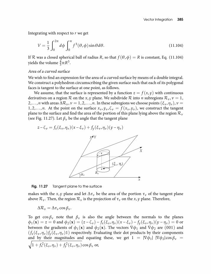
Vector Integration 385
Integrating with respect to r we get
V =13
∫ 2π
0dφ
∫ π
0f 3(θ,φ)sinθdθ. (11.104)
If R was a closed spherical ball of radius R, so that f (θ,φ) = R is constant, Eq. (11.104)yields the volume 4
3πR3.
Area of a curved surfaceWe wish to find an expression for the area of a curved surface by means of a double integral.We construct a polyhedron circumscribing the given surface such that each of its polygonalfaces is tangent to the surface at one point, as follows.
We assume, that the surface is represented by a function z = f (x,y) with continuousderivatives on a regionR on the x,y plane. We subdivideR into n subregionsRν ,ν = 1,2, . . . ,nwith areas ∆Rν ,ν = 1,2, . . . ,n. In these subregions we choose points (ξν ,ην),ν =1,2, . . . ,n. At the point on the surface xν ,yν ,ζν = f (xν ,yν), we construct the tangentplane to the surface and find the area of the portion of this plane lying above the regionRν(see Fig. 11.27). Let βν be the angle that the tangent plane
z − ζν = fx(ξν ,ην)(x − ξν) + fy(ξν ,ην)(y − ην)
Fig. 11.27 Tangent plane to the surface
makes with the x,y plane and let ∆τν be the area of the portion τν of the tangent planeaboveRν . Then, the regionRν is the projection of τν on the x,y plane. Therefore,
∆Rν = ∆τν cosβν .
To get cosβν note that βν is also the angle between the normals to the planesφ1(x) = z = 0 and φ2(x) = (z − ζν) − fx(ξν ,ην)(x − ξν) − fy(ξν ,ην)(y − ην) = 0 orbetween the gradients of φ1(x) and φ2(x). The vectors ∇φ1 and ∇φ2 are (001) and(fx(ξν ,ην)fy(ξν ,ην)1) respectively. Evaluating their dot products by their componentsand by their magnitudes and equating these, we get 1 = |∇φ1| |∇φ2|cosβν =√
1+ f 2x (ξν ,ην) + f
2y (ξν ,ην)cosβν or,
386 An Introduction to Vectors, Vector Operators and Vector Analysis
cosβν =1√
1+ f 2x (ξν ,ην) + f
2y (ξν ,ην)
.
Therefore,
∆τν =√
1+ f 2x (ξν ,ην) + f
2y (ξν ,ην) ·∆Rν .
We form the sum of all these areas
n∑ν=1
∆τν
and let n → ∞ and simultaneously the diameter of the largest subdivision tend to zero.This sum will then have the limit, independent of the way we subdivideR,
A=
∫ ∫R
√1+ f 2
x + f 2y dR. (11.105)
We use this integral to define the area of the given surface. Note that if the surface happensto be a plane surface, for example z = f (x,y) = 0, we have
A=
∫ ∫RdR,
which agrees with our definition of the area of a planar region. Sometimes we call
dσ =√
1+ f 2x + f 2
y dR=√
1+ f 2x + f 2
y dxdy
the element of area of the surface z = f (x,y). The area integral can be writtensymbolically in the form
A=
∫ ∫Rdσ .
Exercise Evaluate the area of a spherical surface of radius R.
Solution The equation to the hemispherical surface of radius R can be written in thez = f (x,y) form as
z =√R2 − x2 − y2.
Vector Integration 387
We find
∂z∂x
= − x√R2 − x2 − y2
;∂z∂y
= −y√
R2 − x2 − y2.
The area of the full sphere is therefore given by the integral
A= 2R∫ ∫
dxdy√R2 − x2 − y2
,
where the region of integration is the circle of radius R lying in the x,y plane with itsorigin at the center. Introducing polar coordinates and resolving into single integralswe get
A= 2R∫ 2π
0dθ
∫ R
0
rdr√R2 − r2
= 4πR∫ R
0
rdr√R2 − r2
= 4πR2,
where the last integral on the right can be easily evaluated by substitutingR2 − r2 = u2.
If the equation to the surface is given in the form φ(x,y,z) = 0 then we get anotherexpression for its area. Assuming this equation gives implicit dependence of z onindependent variables x and y, and also that φz , 0, we get
dφ
dx=∂φ
∂x+∂φ
∂z∂z∂x
= 0; or, fx =∂z∂x
= −φx
φz.
Similarly,
fy =∂z∂y
= −φyφz
.
These two relations at once give the expression
A=
∫ ∫R
√φ2x +φ
2y +φ
2z
∣∣∣∣∣ 1φz
∣∣∣∣∣dxdy (11.106)
for the area where the regionR is again the projection of the surface on the x,y plane.If, instead of z = z(x,y), the surface was given by x = x(y,z) then the expression for
area would be
A=
∫ ∫ √1+ x2
y + x2zdydz =
∫ ∫ √φ2x +φ
2y +φ
2z
∣∣∣∣∣ 1φx
∣∣∣∣∣dydz, (11.107)
388 An Introduction to Vectors, Vector Operators and Vector Analysis
or, if the surface was given by y = y(z,x) then the expression for area would be
A=
∫ ∫ √1+ y2
x + y2z dzdx =
∫ ∫ √φ2x +φ
2y +φ
2z
∣∣∣∣∣∣ 1φy
∣∣∣∣∣∣dzdx. (11.108)
Equations (11.106), (11.107), (11.108) define the same area. To see this, apply thetransformation
x = x(y,z), y = y,
where x = x(y,z) is obtained by solving the equation φ(x,y,z) = 0, to the integral inEq. (11.106). The Jacobian determinant is
d(x,y)d(y,z)
=φzφx
,
so that∫ ∫R
√φ2x +φ
2y +φ
2z
∣∣∣∣∣ 1φz
∣∣∣∣∣dxdy = ∫ ∫R
√φ2x +φ
2y +φ
2z
∣∣∣∣∣ 1φx
∣∣∣∣∣dydz,where R is the projection of the surface on the y,z plane.
We can get rid of any special assumption about the relation of the surface and thecoordinate system, by representing the surface in the parametric form
x = φ(u,v), y = ψ(u,v), z = χ(u,v)
and expressing the area of the surface as an integral over the appropriate parameter domain.Then, a definite region in the (u,v) plane corresponds to the surface. Without going intothe details we simply state the expression for the area of a surface in terms of its parametricdescription.
A=
∫ ∫R
√(φuψv −ψuφv)2 + (ψuχv −χuψv)2 + (χuφv −φuχv)2dudv. (11.109)
Exercise For a given surface parameterized by u,v show that
A=
∫ ∫ √EG −F2dudv (11.110)
and that the element of area
dσ =√EG −F2dudv,
where E,F,G are the coefficients of the line element given by Eqs (10.66), (10.67), (10.68).
Vector Integration 389
Hint A simple calculation shows
EG −F2 = (φuψv −ψuφv)2 + (ψuχv −χuψv)2 + (χuφv −φuχv)2.
Exercise Using the parametric representation of a sphere of radius R via the sphericalpolar coordinates θ,φ, 0 ≤ θ ≤ π, 0 ≤ φ ≤ 2π, show that
dσ = R2 sinθdθdφ
and hence show that the area of this sphere is 4πR2.
We can apply Eq. (11.110) to the surface of revolution formed by rotating the curve z =φ(x), cut off by the two planes z = z0 and z = z1, about the z-axis. Referring the surfaceto polar coordinates r,θ in the x,y plane as parameters, we get
x = r cosθ, y = r sinθ, z = φ(√x2 + y2) = φ(r).
Here, r coordinate of a point on the curve is the radius of the circle it traces out as it rotatesabout the z-axis. This gives
E = 1+φ′2(r), F = 0, G = r2
so that the area is given by∫ 2π
0dθ
∫ r1
r0
r√
1+φ′2(r)dr = 2π∫ r1
r0
r√
1+φ′2(r)dr.
Recognizing√
1+φ′2(r)dr = ds where s is the arc length parameter of the curve z =φ(r) we can express the area of the surface of revolution in the form
2π∫ s1
s0
rds,
where r is the distance from the z-axis to the point on the rotating curve correspondingto s.
Exercise Use the above integral with respect to the arc length parameter to calculatethe surface area of the torus obtained by rotating the circle (x − a)2 + z2 = r2 about thez-axis.
Solution We introduce arc length as parameter, so that the distance u of a point on thecircle from the z-axis is given by u = a+ r cos(s/r). The area is, therefore,
2π∫ 2πr
0uds = 2π
∫ 2πr
0
(a+ r cos
sr
)ds = 2πa · 2πr.
390 An Introduction to Vectors, Vector Operators and Vector Analysis
The area of the torus is therefore equal to the product of the circumference of thegenerating circle and the length of the path traced out by the center of the circle.
11.4.8 Physical applications of multiple integrals
Applications of multiple integrals to science and engineering are ubiquitous and are foundin all parts of it and in all kinds of situations. An exposure to it can really be obtainedthrough a wide verity of books and literature on various subjects and also while practisingdifferent professions. Here, we give a brief account of some applications to mechanics.
Consider a distribution of n particles with respect to a cartesian coordinate system,whose masses and positions are given by mν , (xν ,yν ,zν), ν = 1,2, . . . ,n. Then, themoments of such a mass distribution with respect to x,y y,z and z,x planes are defined tobe Tz =
∑nν=1mνzν , Tx =
∑nν=1mνxν and Ty =
∑nν=1mνyν respectively. When we deal
with a continuous distribution of mass with density µ(x,y,z) in a region R in space or asurface S or a curve γ , going through the same limiting process as we did while definingmultiple integrals, The corresponding moments go over to
Tx =
∫ ∫ ∫Rµxdxdydz, Ty =
∫ ∫ ∫Rµydxdydz, Tz =
∫ ∫ ∫Rµzdxdydz, (11.111)
and we call these the moments of a volume distribution.If the mass is continuously distributed over a surface S given by x = φ(u,v),
y = ψ(u,v), z = χ(u,v) with density µ(u,v), we define the moments of the surfacedistribution by expressions
Tx =
∫ ∫Sµxdσ =
∫ ∫Rµx√EG −F2dudv,
Ty =
∫ ∫Sµydσ =
∫ ∫Rµy√EG −F2dudv,
Tz =
∫ ∫Sµzdσ =
∫ ∫Rµz√EG −F2dudv. (11.112)
Finally, the moments of a curve x(s),y(s),z(s) in space with mass density µ(s) aredefined by
Tx =
∫ s1
s0
µxds, Ty =
∫ s1
s0
µyds, Tz =
∫ s1
s0
µzds,
where s denotes the arc length.The center of mass of a continuous mass distribution over a region R, with total mass
M, is defined as the point with coordinates
ξ =TxM
, η =TyM
, ζ =TzM
. (11.113)
Vector Integration 391
That is, the center of mass has the coordinates, ξ,η,ζ= 1M
∫ ∫ ∫Rµx,y,zdxdydzwhere
M =∫ ∫ ∫
Rµdxdydz.If the mass distribution is homogeneous, that is, µ = constant the center of mass of
the region is called its centroid. The centroid is clearly independent of the choice of theconstant positive value of the mass density. Thus, the centroid becomes a geometricalconcept associated only with the shape of the region R, independent of the massdistribution.
Exercise Find the center of mass of a homogeneous hemispherical region H with massdensity 1.
Solution The region is given by x2 + y2 + z2 ≤ 1 ; z ≥ 0. The two moments Tx and Tyare zero as the respective integrations with respect to x and y vanish. For
Tz =
∫ ∫ ∫Hzdxdydz,
we introduce cylindrical coordinates (r,θ,z) via the equations
z = z, x = r cosθ, y = r sinθ
to get
Tz =
∫ 1
0zdz
∫ √1−z2
0rdr
∫ 2π
0dθ = 2π
∫ 1
0
1− z2
2zdz =
π4
.
Since the total mass is 2π3 , the coordinates of the center of mass are (0,0, 3
8).
Exercise Find the center of mass of a hemispherical surface of unit radius over which amass of unit density is uniformly distributed.
Solution For the parametric representation
x = sinθ cosφ, y = sinθ sinφ z = cosθ
we get, for the surface element,
dσ =√EG −F2dθdφ = sinθdθdφ.
This leads to Tx = 0 = Ty because these involve integrating cosφ and sinφ over a singleperiod and
Tz =
∫ π/2
0sinθ cosθdθ
∫ 2π
0dφ = π.
Since the total mass is 2π we see that the coordinates of the center of mass are (0,0, 12).
392 An Introduction to Vectors, Vector Operators and Vector Analysis
Moment of inertiaThe moment of inertia plays the role of mass for the rotational motion of a rigid body. Thekinetic energy of a body rotating uniformly about an axis equals the product of the squareof the rotational velocity and the moment of inertia. The moment of inertia of a continuousmass distribution with density µ(x) = µ(x,y,z) over a regionR with respect to the x-axisis given by
Ix =
∫ ∫ ∫Rµ(y2 + z2)dxdydz.
This is simply integrating over the distance of every point (x,y,z) in R from the x-axismultiplied by the mass density µ(x,y,z). The moments of inertia about the other two axesare defined similarly. The moment of inertia about a point, say the origin is defined to be∫ ∫ ∫
Rµ(x2 + y2 + z2)dxdydz
and the moment of inertia with respect to a plane say the y,z plane is∫ ∫ ∫Rµx2dxdydz.
A complete description of the arbitrary rotational motion of a rigid body requires the socalled products of inertia
Ixy = −∫ ∫ ∫
Rµxydxdydz = Iyx,
Iyz = −∫ ∫ ∫
Rµyzdxdydz = Izy ,
Izx = −∫ ∫ ∫
Rµzxdxdydz = Ixz. (11.114)
The three quantities Ix,Iy ,Iz and the six products of inertia are sufficient to describearbitrary rotational motion of a rigid body. These nine quantities, written as a symmetricmatrix, are collectively called the moment of inertia tensor. The mutually perpendicularaxes with respect to which the moment of inertia tensor becomes diagonal are called theprincipal axes. Generally, these are determined by the symmetry elements of the rigid body.
The moment of inertia with respect to an axis parallel to x-axis and passing through thepoint (ξ,η,ζ), is given by the expression∫ ∫ ∫
Rµ[(y − η)2 + (z − ζ)2]dxdydz,
Vector Integration 393
obtained by shifting the origin to (ξ,η,ζ).If we let (ξ,η,ζ) be the coordinates of the center of mass and use Eq. (11.113) for the
coordinates of the center of mass, we immediately get∫ ∫ ∫Rµ(y2 + z2)dxdydz
=
∫ ∫ ∫Rµ[(y − η)2 + (z − ζ)2]dxdydz+ (η2 + ζ2)
∫ ∫ ∫Rµdxdydz.
Since any arbitrary axis of rotation can be chosen to be the x-axis, the result we have gotcan be expressed as follows.
The moment of inertia of a rigid body with respect to an arbitrary axis of rotation isequal to the moment of inertia of the body about a parallel axis through its center of massplus the product of the total mass and the square of the distance between the center of massand the axis of rotation.
Finally, the moment of inertia of a surface distribution, with respect to the x-axis, isgiven by∫ ∫
Sµ(y2 + z2)dσ ,
where µ(u,v) is the continuous function of two parameters u and v.
Exercise Find the moment of inertia of a sphere of unit radius and unit density andoccupying region V , about any axis through its center at the origin.
Solution By symmetry the moment of inertia about any axis through the origin is
I =
∫ ∫ ∫V(y2 + z2)dxdydz,
=
∫ ∫ ∫V(x2 + z2)dxdydz,
=
∫ ∫ ∫V(x2 + y2)dxdydz. (11.115)
Adding these three integrals we obtain,
3I = 2∫ ∫ ∫
V(x2 + y2 + z2)dxdydz.
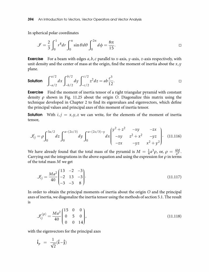
394 An Introduction to Vectors, Vector Operators and Vector Analysis
In spherical polar coordinates
I =23
∫ 1
0r4dr
∫ π
0sinθdθ
∫ 2π
0dφ =
8π15
.
Exercise For a beam with edges a,b,c parallel to x-axis, y-axis, z-axis respectively, withunit density and the center of mass at the origin, find the moment of inertia about the x,yplane.
Solution∫ a/2
−a/2dx
∫ b/2
−b/2dy
∫ c/2
−c/2z2dz = ab
c3
12.
Exercise Find the moment of inertia tensor of a right triangular pyramid with constantdensity ρ shown in Fig. 11.25 about the origin O. Diagonalize this matrix using thetechnique developed in Chapter 2 to find its eigenvalues and eigenvectors, which definethe principal values and principal axes of this moment of inertia tensor.
Solution With i, j = x,y,z we can write, for the elements of the moment of inertiatensor,
Iij = ρ
∫ 3a/2
0dz
∫ a−(2z/3)
0dy
∫ a−(2z/3)−y
0dx
y2 + z2 −xy −zx−xy z2 + x2 −yz−zx −yz x2 + y2
· (11.116)
We have already found that the total mass of the pyramid is M = 14a
3ρ, or, ρ = 4Ma3 .
Carrying out the integrations in the above equation and using the expression for ρ in termsof the total massM we get
Iij =Ma2
40
13 −2 −3−2 13 −3−3 −3 8
· (11.117)
In order to obtain the principal moments of inertia about the origin O and the principalaxes of inertia, we diagonalize the inertia tensor using the methods of section 5.1. The resultis
I(p)ij =
Ma2
40
15 0 00 5 00 0 14
, (11.118)
with the eigenvectors for the principal axes
ip =1√
2(i− j)
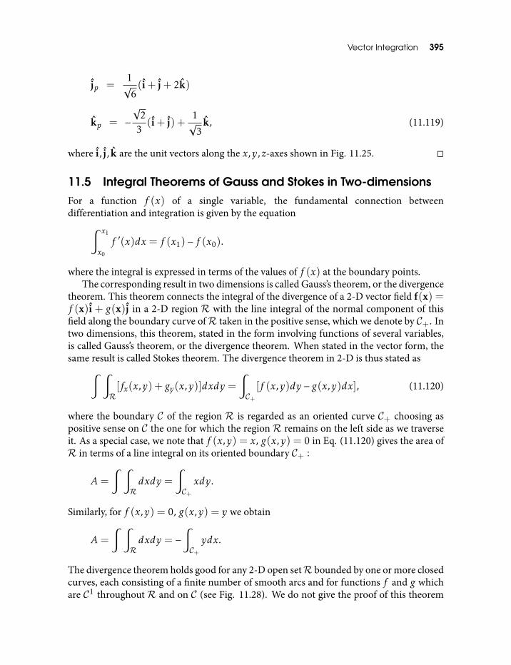
Vector Integration 395
jp =1√
6(i+ j+ 2k)
kp = −√
23(i+ j) +
1√
3k, (11.119)
where i, j, k are the unit vectors along the x,y,z-axes shown in Fig. 11.25.
11.5 Integral Theorems of Gauss and Stokes in Two-dimensionsFor a function f (x) of a single variable, the fundamental connection betweendifferentiation and integration is given by the equation∫ x1
x0
f ′(x)dx = f (x1)− f (x0).
where the integral is expressed in terms of the values of f (x) at the boundary points.The corresponding result in two dimensions is called Gauss’s theorem, or the divergence
theorem. This theorem connects the integral of the divergence of a 2-D vector field f(x) =f (x)i + g(x)j in a 2-D region R with the line integral of the normal component of thisfield along the boundary curve ofR taken in the positive sense, which we denote by C+. Intwo dimensions, this theorem, stated in the form involving functions of several variables,is called Gauss’s theorem, or the divergence theorem. When stated in the vector form, thesame result is called Stokes theorem. The divergence theorem in 2-D is thus stated as∫ ∫
R[fx(x,y) + gy(x,y)]dxdy =
∫C+[f (x,y)dy − g(x,y)dx], (11.120)
where the boundary C of the region R is regarded as an oriented curve C+ choosing aspositive sense on C the one for which the region R remains on the left side as we traverseit. As a special case, we note that f (x,y) = x, g(x,y) = 0 in Eq. (11.120) gives the area ofR in terms of a line integral on its oriented boundary C+ :
A=
∫ ∫Rdxdy =
∫C+xdy.
Similarly, for f (x,y) = 0, g(x,y) = y we obtain
A=
∫ ∫Rdxdy = −
∫C+ydx.
The divergence theorem holds good for any 2-D open setR bounded by one or more closedcurves, each consisting of a finite number of smooth arcs and for functions f and g whichare C1 throughout R and on C (see Fig. 11.28). We do not give the proof of this theorem
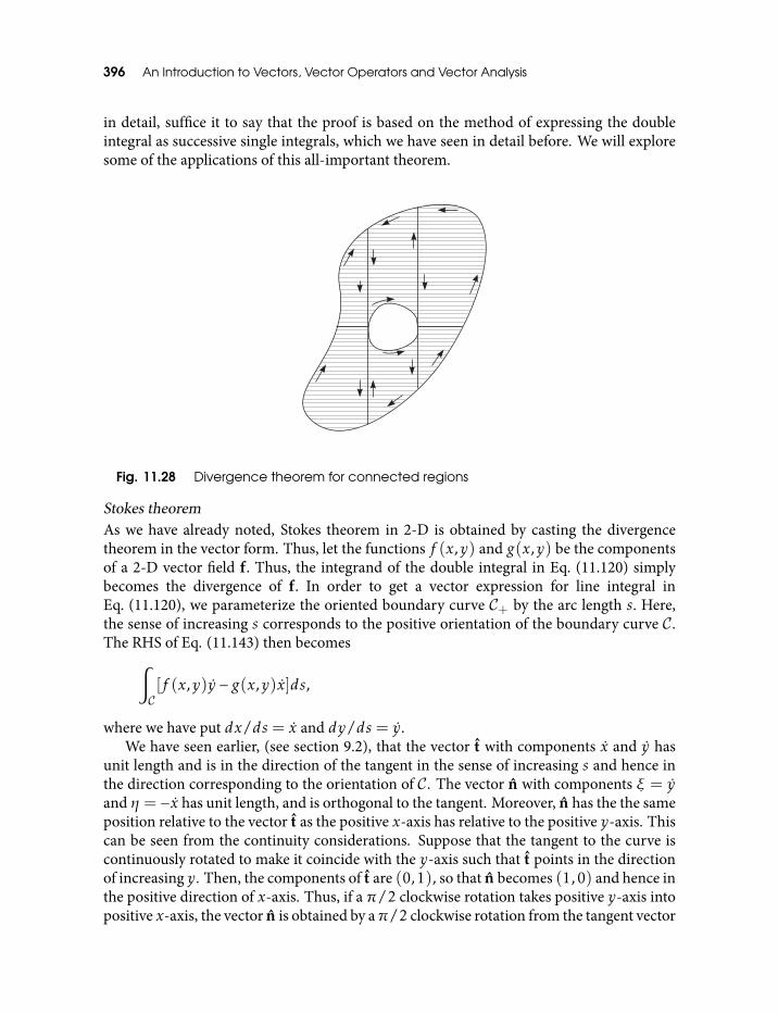
396 An Introduction to Vectors, Vector Operators and Vector Analysis
in detail, suffice it to say that the proof is based on the method of expressing the doubleintegral as successive single integrals, which we have seen in detail before. We will exploresome of the applications of this all-important theorem.
Fig. 11.28 Divergence theorem for connected regions
Stokes theoremAs we have already noted, Stokes theorem in 2-D is obtained by casting the divergencetheorem in the vector form. Thus, let the functions f (x,y) and g(x,y) be the componentsof a 2-D vector field f. Thus, the integrand of the double integral in Eq. (11.120) simplybecomes the divergence of f. In order to get a vector expression for line integral inEq. (11.120), we parameterize the oriented boundary curve C+ by the arc length s. Here,the sense of increasing s corresponds to the positive orientation of the boundary curve C.The RHS of Eq. (11.143) then becomes∫
C[f (x,y)y − g(x,y)x]ds,
where we have put dx/ds = x and dy/ds = y.We have seen earlier, (see section 9.2), that the vector t with components x and y has
unit length and is in the direction of the tangent in the sense of increasing s and hence inthe direction corresponding to the orientation of C. The vector n with components ξ = yand η = −x has unit length, and is orthogonal to the tangent. Moreover, n has the the sameposition relative to the vector t as the positive x-axis has relative to the positive y-axis. Thiscan be seen from the continuity considerations. Suppose that the tangent to the curve iscontinuously rotated to make it coincide with the y-axis such that t points in the directionof increasing y. Then, the components of t are (0,1), so that n becomes (1,0) and hence inthe positive direction of x-axis. Thus, if a π/2 clockwise rotation takes positive y-axis intopositive x-axis, the vector n is obtained by aπ/2 clockwise rotation from the tangent vector
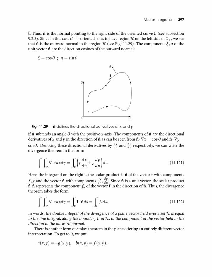
Vector Integration 397
t. Thus, n is the normal pointing to the right side of the oriented curve C (see subsection9.2.5). Since in this case C+ is oriented so as to have regionR on the left side of C+, we seethat n is the outward normal to the regionR (see Fig. 11.29). The components ξ,η of theunit vector n are the direction cosines of the outward normal:
ξ = cosθ ; η = sinθ
Fig. 11.29 n defines the directional derivatives of x and y
if n subtends an angle θ with the positive x-axis. The components of n are the directionalderivatives of x and y in the direction of n as can be seen from n ·∇x = cosθ and n ·∇y =sinθ. Denoting these directional derivatives by dx
dn and dydn respectively, we can write the
divergence theorem in the form:∫ ∫R∇ · fdxdy =
∫C
(fdxdn
+ gdy
dn
)ds. (11.121)
Here, the integrand on the right is the scalar product f · n of the vector f with componentsf ,g and the vector n with components dx
dn , dydn . Since n is a unit vector, the scalar productf · n represents the component fn of the vector f in the direction of n. Thus, the divergencetheorem takes the form∫ ∫
R∇ · fdxdy =
∫C
f · nds =∫Cfnds. (11.122)
In words, the double integral of the divergence of a plane vector field over a set R is equalto the line integral, along the boundary C ofR, of the component of the vector field in thedirection of the outward normal.
There is another form of Stokes theorem in the plane offering an entirely different vectorinterpretation. To get to it, we put
a(x,y) = −g(x,y), b(x,y) = f (x,y).
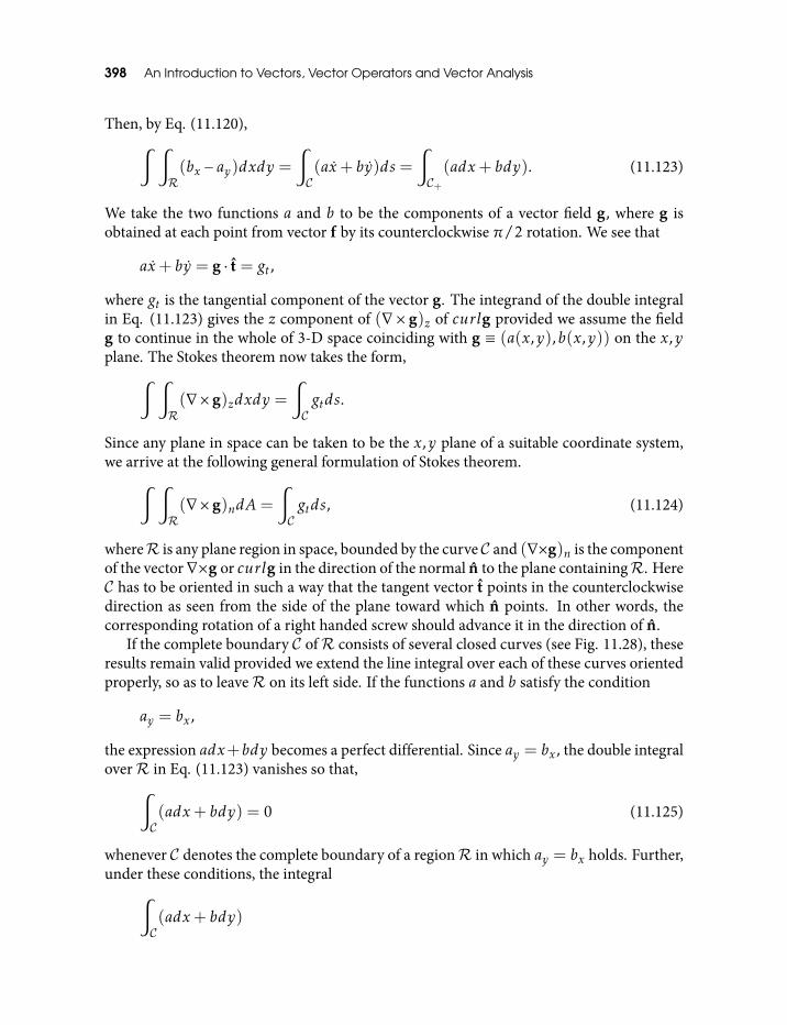
398 An Introduction to Vectors, Vector Operators and Vector Analysis
Then, by Eq. (11.120),∫ ∫R(bx − ay)dxdy =
∫C(ax+ by)ds =
∫C+(adx+ bdy). (11.123)
We take the two functions a and b to be the components of a vector field g, where g isobtained at each point from vector f by its counterclockwise π/2 rotation. We see that
ax+ by = g · t = gt,
where gt is the tangential component of the vector g. The integrand of the double integralin Eq. (11.123) gives the z component of (∇× g)z of curlg provided we assume the fieldg to continue in the whole of 3-D space coinciding with g ≡ (a(x,y),b(x,y)) on the x,yplane. The Stokes theorem now takes the form,∫ ∫
R(∇× g)zdxdy =
∫Cgtds.
Since any plane in space can be taken to be the x,y plane of a suitable coordinate system,we arrive at the following general formulation of Stokes theorem.∫ ∫
R(∇× g)ndA=
∫Cgtds, (11.124)
whereR is any plane region in space, bounded by the curve C and (∇×g)n is the componentof the vector∇×g or curlg in the direction of the normal n to the plane containingR. HereC has to be oriented in such a way that the tangent vector t points in the counterclockwisedirection as seen from the side of the plane toward which n points. In other words, thecorresponding rotation of a right handed screw should advance it in the direction of n.
If the complete boundary C ofR consists of several closed curves (see Fig. 11.28), theseresults remain valid provided we extend the line integral over each of these curves orientedproperly, so as to leaveR on its left side. If the functions a and b satisfy the condition
ay = bx,
the expression adx+bdy becomes a perfect differential. Since ay = bx, the double integraloverR in Eq. (11.123) vanishes so that,∫
C(adx+ bdy) = 0 (11.125)
whenever C denotes the complete boundary of a regionR in which ay = bx holds. Further,under these conditions, the integral∫
C(adx+ bdy)
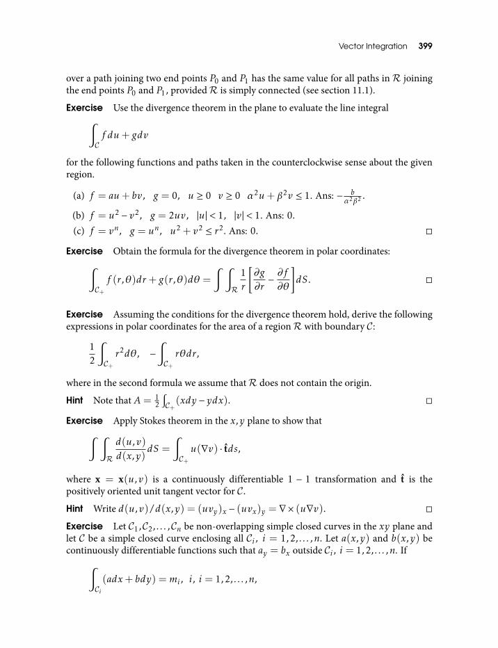
Vector Integration 399
over a path joining two end points P0 and P1 has the same value for all paths in R joiningthe end points P0 and P1, providedR is simply connected (see section 11.1).
Exercise Use the divergence theorem in the plane to evaluate the line integral∫Cf du+ gdv
for the following functions and paths taken in the counterclockwise sense about the givenregion.
(a) f = au+ bv, g = 0, u ≥ 0 v ≥ 0 α2u+ β2v ≤ 1. Ans: − bα2β2 .
(b) f = u2 − v2, g = 2uv, |u| < 1, |v| < 1. Ans: 0.
(c) f = vn, g = un, u2 + v2 ≤ r2. Ans: 0.
Exercise Obtain the formula for the divergence theorem in polar coordinates:∫C+f (r,θ)dr + g(r,θ)dθ =
∫ ∫R
1r
[∂g
∂r−∂f
∂θ
]dS.
Exercise Assuming the conditions for the divergence theorem hold, derive the followingexpressions in polar coordinates for the area of a regionR with boundary C:
12
∫C+r2dθ, −
∫C+rθdr,
where in the second formula we assume thatR does not contain the origin.
Hint Note that A= 12
∫C+(xdy − ydx).
Exercise Apply Stokes theorem in the x,y plane to show that∫ ∫R
d(u,v)d(x,y)
dS =
∫C+u(∇v) · tds,
where x = x(u,v) is a continuously differentiable 1 − 1 transformation and t is thepositively oriented unit tangent vector for C.
Hint Write d(u,v)/d(x,y) = (uvy)x − (uvx)y = ∇× (u∇v).
Exercise Let C1,C2, . . . ,Cn be non-overlapping simple closed curves in the xy plane andlet C be a simple closed curve enclosing all Ci , i = 1,2, . . . ,n. Let a(x,y) and b(x,y) becontinuously differentiable functions such that ay = bx outside Ci , i = 1,2, . . . ,n. If∫
Ci(adx+ bdy) =mi , i, i = 1,2, . . . ,n,
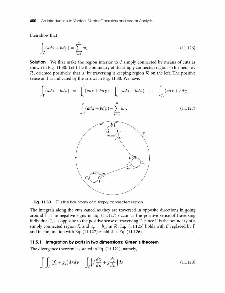
400 An Introduction to Vectors, Vector Operators and Vector Analysis
then show that∫C(adx+ bdy) =
n∑i=1
mi . (11.126)
Solution We first make the region interior to C simply connected by means of cuts asshown in Fig. 11.30. Let Γ be the boundary of the simply connected region so formed, sayR, oriented positively, that is, by traversing it keeping region R on the left. The positivesense on Γ is indicated by the arrows in Fig. 11.30. We have,∫
Γ
(adx+ bdy) =
∫C(adx+ bdy)−
∫C1
(adx+ bdy)− · · · −∫Cn(adx+ bdy)
=
∫C(adx+ bdy)−
n∑i=1
mi . (11.127)
Fig. 11.30 Γ is the boundary of a simply connected region
The integrals along the cuts cancel as they are traversed in opposite directions in goingaround Γ . The negative signs in Eq. (11.127) occur as the positive sense of traversingindividual Cis is opposite to the positive sense of traversing Γ . Since Γ is the boundary of asimply connected region R and ay = bx, in R, Eq. (11.125) holds with C replaced by Γ
and in conjunction with Eq. (11.127) establishes Eq. (11.126).
11.5.1 Integration by parts in two dimensions: Green’s theorem
The divergence theorem, as stated in Eq. (11.121), namely,∫ ∫R(fx+ gy)dxdy =
∫C
(fdxdn
+ gdy
dn
)ds (11.128)
Vector Integration 401
combined with the rule for differentiating a product immediately gives a prescription forintegrating by parts that is basic to the theory of partial differential equations. We substitutefor both f and g a product of functions, namely, f (x,y) = a(x,y)u(x,y) and g(x,y) =b(x,y)v(x,y), where the functions a,b,u,v are C1 inR as well as on C. Since
fx+ gy = (aux+ bvy) + (axu+ byv),
we can write Eq. (11.128) as∫ ∫R(aux+ bvy)dxdy =
∫C
(audxdn
+ bvdy
dn
)ds −
∫ ∫R(axu+ byv)dxdy. (11.129)
To get Green’s first theorem, we impose u = v, a = ωx and b = ωy for some ω(x,y). Weassume that u is C1 while ω has continuous second derivatives in the closure of R. Thistransforms Eq. (11.129) into∫ ∫
R(uxωx+uyωy)dxdy =
∫Cu
(ωxdxdn
+ωydy
dn
)ds−
∫ ∫Ru(ωxx+ωyy)dxdy.
Recognizing
ωxx+ωyy = ∇2ω ≡ ∆ω
and that dxdn and dydn are the direction cosines of the outward normal to the boundary C of
R so that
ωxdxdn
+ωydy
dn=dωdn
is the directional derivative ofω in the direction of the outward normal to C, we obtain, forGreen’s first theorem,∫ ∫
R(uxωx+ uyωy)dxdy =
∫Cudωdnds −
∫ ∫Ru∆ωdxdy. (11.130)
If in addition u has continuous second derivatives, we get from Eq. (11.130), byinterchanging the roles of u and ω the equation∫ ∫
R(ωxux+ωyuy)dxdy =
∫Cωdudnds −
∫ ∫Rω∆udxdy.
Subtracting the two equations gives an equation symmetric in u and ω known as Green’ssecond theorem :∫ ∫
R(ω∆u −u∆ω)dxdy =
∫C
(udωdn−ωdu
dn
)ds. (11.131)
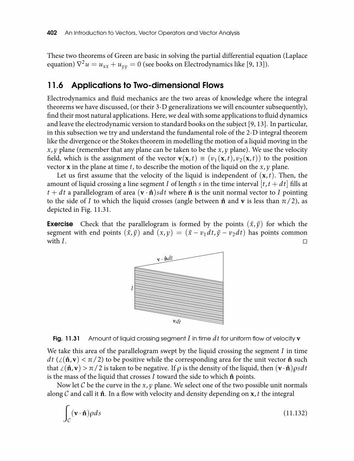
402 An Introduction to Vectors, Vector Operators and Vector Analysis
These two theorems of Green are basic in solving the partial differential equation (Laplaceequation) ∇2u = uxx+ uyy = 0 (see books on Electrodynamics like [9, 13]).
11.6 Applications to Two-dimensional FlowsElectrodynamics and fluid mechanics are the two areas of knowledge where the integraltheorems we have discussed, (or their 3-D generalizations we will encounter subsequently),find their most natural applications. Here, we deal with some applications to fluid dynamicsand leave the electrodynamic version to standard books on the subject [9, 13]. In particular,in this subsection we try and understand the fundamental role of the 2-D integral theoremlike the divergence or the Stokes theorem in modelling the motion of a liquid moving in thex,y plane (remember that any plane can be taken to be the x,y plane). We use the velocityfield, which is the assignment of the vector v(x, t) ≡ (v1(x, t),v2(x, t)) to the positionvector x in the plane at time t, to describe the motion of the liquid on the x,y plane.
Let us first assume that the velocity of the liquid is independent of (x, t). Then, theamount of liquid crossing a line segment I of length s in the time interval [t, t+ dt] fills att + dt a parallelogram of area (v · n)sdt where n is the unit normal vector to I pointingto the side of I to which the liquid crosses (angle between n and v is less than π/2), asdepicted in Fig. 11.31.
Exercise Check that the parallelogram is formed by the points (x, y) for which thesegment with end points (x, y) and (x,y) = (x − v1dt, y − v2dt) has points commonwith I .
Fig. 11.31 Amount of liquid crossing segment I in time dt for uniform flow of velocity v
We take this area of the parallelogram swept by the liquid crossing the segment I in timedt (∠(n,v) < π/2) to be positive while the corresponding area for the unit vector n suchthat ∠(n,v) > π/2 is taken to be negative. If ρ is the density of the liquid, then (v · n)ρsdtis the mass of the liquid that crosses I toward the side to which n points.
Now let C be the curve in the x,y plane. We select one of the two possible unit normalsalong C and call it n. In a flow with velocity and density depending on x, t the integral∫
C(v · n)ρds (11.132)
Vector Integration 403
represents mass of the liquid crossing C in unit time toward the side of C to which n points.This follows by approximating C by a polygon and the flow for which the velocity is constantacross each side of the polygon.
If C is the boundary of a region R and if n is the outward normal, the integralrepresents the mass of the liquid leaving R in unit time. Applying the divergence theoremas in Eq. (11.122)we can express the flow through C as a double integral∫
C(v · n)ρds =
∫C(ρv) · nds =
∫ ∫R∇ · (ρv)dxdy. (11.133)
We can compare this flow of mass through C out of R with the change in mass containedinR. The total mass of the liquid contained in the regionR at time t is∫ ∫
Rρ(x, t)dxdy.
Thus, in unit time, the loss of mass fromR is given by
− ddt
∫ ∫Rρ(x, t)dxdy = −
∫ ∫R
∂ρ
∂t(x, t)dxdy.
If we assume that the mass is conserved, then mass can only be lost from R by passingthrough the boundary C. Hence, by Eq. (11.133) we have∫ ∫
R(∇ · (ρv) +
∂ρ
∂t)dxdy = 0. (11.134)
Since this identity holds for arbitraryR, if we progressively reduce the area ofR the integralwill have the value given by the product of the integrand evaluated at some arbitrary pointin R and the area of R. Since area of R > 0, the integrand must vanish at all points atwhich the velocity field is defined. Stated more rigorously, if we divide Eq. (11.134) by thearea ofR then in the limit as area ofR tends to zero, we get
∇ · (ρv) +∂ρ
∂t= 0. (11.135)
This differential equation expresses the law of conservation of mass in the flow. In terms ofthe components (v1,v2) of the velocity vector we can write Eq. (11.135) as
∂ρ
∂t+ v1
∂ρ
∂x+ v2
∂ρ
∂y+ ρ
(∂v1
∂x+∂v2
∂y
)= 0. (11.136)
An important special case is that of an incompressible homogeneous liquid in which thedensity ρ has a constant value independent of location and time. In this case, Eqs (11.135),(11.136) reduce to an equation involving the velocity vector alone:
404 An Introduction to Vectors, Vector Operators and Vector Analysis
∇ · v =∂v1
∂x+∂v2
∂y= 0. (11.137)
Combining Eqs (11.133) and (11.137) we see that the total amount of an incompressibleliquid crossing a closed curve C is zero:∫
C(v · n)ds = 0. (11.138)
Stokes theorem, in the form of Eq. (11.124) applied to the vector field v has alsointeresting consequences for the liquid flow. The integral over a closed oriented curve Cnamely,∫
Cv · tds
where t is the unit tangent vector corresponding to the orientation of C, is called thecirculation of the liquid around C. By stokes theorem, this circulation is equal to thedouble integral∫ ∫
R(∇× v)zdxdy
over the enclosed regionR. Hence, the quantity
(∇× v)z =∂v2
∂x− ∂v1
∂y, (11.139)
called the vorticity of the motion, measures the density of circulation at the pointx ≡ (x,y) in the sense that the area integral of the vorticity gives the circulation aroundthe boundary. A flow is called irrotational if the vorticity vanishes everywhere, that is, if
(∇× v)z =∂v2
∂x− ∂v1
∂y= 0. (11.140)
By stokes theorem, the circulation around a closed curve C vanishes if C is the boundary ofa region where the motion is irrotational. Since Eq. (11.140) is the condition forv1dx + v2dy to be a perfect differential, there exists for an irrotational flow in everysimply connected region a scalar valued function φ(x, t) such that
v(x) = −∇φ(x). (11.141)
The scalar φ, which is determined within a constant, is called a velocity potential.The irrotational motion of an incompressible homogeneous liquid satisfies both,
Eqs (11.137) and (11.140). Combining these, we find that the velocity potential is asolution of Laplace’s equation :
∆φ = φxx+φyy = 0.
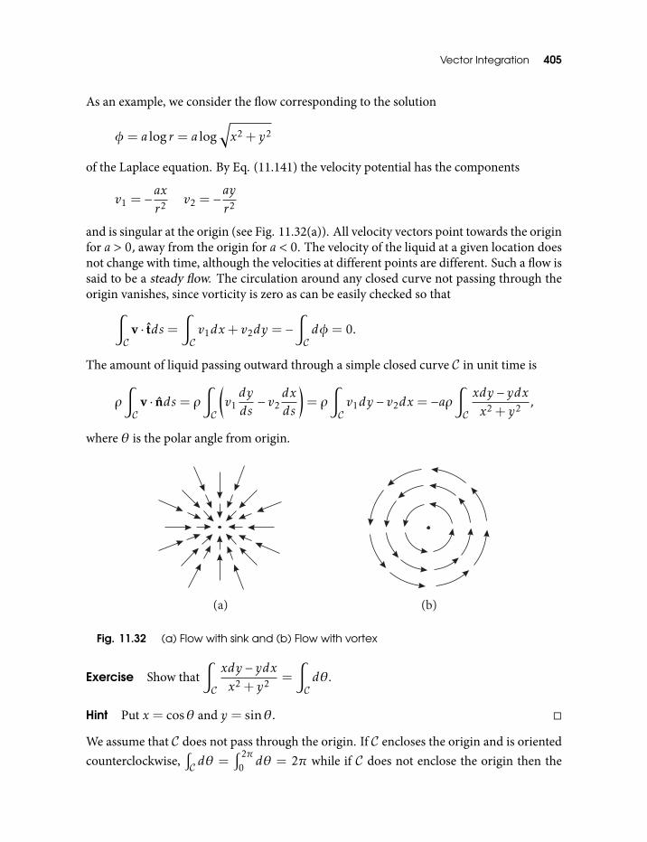
Vector Integration 405
As an example, we consider the flow corresponding to the solution
φ = a logr = a log√x2 + y2
of the Laplace equation. By Eq. (11.141) the velocity potential has the components
v1 = −ax
r2 v2 = −ay
r2
and is singular at the origin (see Fig. 11.32(a)). All velocity vectors point towards the originfor a > 0, away from the origin for a < 0. The velocity of the liquid at a given location doesnot change with time, although the velocities at different points are different. Such a flow issaid to be a steady flow. The circulation around any closed curve not passing through theorigin vanishes, since vorticity is zero as can be easily checked so that∫
Cv · tds =
∫Cv1dx+ v2dy = −
∫Cdφ = 0.
The amount of liquid passing outward through a simple closed curve C in unit time is
ρ
∫C
v · nds = ρ
∫C
(v1dy
ds− v2
dxds
)= ρ
∫Cv1dy − v2dx = −aρ
∫C
xdy − ydxx2 + y2 ,
where θ is the polar angle from origin.
Fig. 11.32 (a) Flow with sink and (b) Flow with vortex
Exercise Show that∫C
xdy − ydxx2 + y2 =
∫Cdθ.
Hint Put x = cosθ and y = sinθ.
We assume that C does not pass through the origin. If C encloses the origin and is orientedcounterclockwise,
∫C dθ =
∫ 2π0 dθ = 2π while if C does not enclose the origin then the
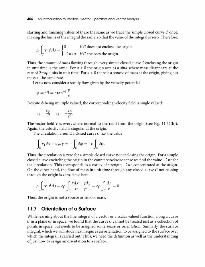
406 An Introduction to Vectors, Vector Operators and Vector Analysis
starting and finishing values of θ are the same as we trace the simple closed curve C once,making the limits of the integral the same, so that the value of the integral is zero. Therefore,
ρ
∫C
v · nds =
0 if C does not enclose the origin
−2πaρ if C encloses the origin.
Thus, the amount of mass flowing through every simple closed curve C enclosing the originin unit time is the same. For a > 0 the origin acts as a sink where mass disappears at therate of 2πaρ units in unit time. For a < 0 there is a source of mass at the origin, giving outmass at the same rate.
Let us now consider a steady flow given by the velocity potential
φ = cθ = c tan−1 y
x.
Despite φ being multiple valued, the corresponding velocity field is single valued:
v1 =cy
r2 v2 = −cx
r2 .
The vector field v is everywhere normal to the radii from the origin (see Fig. 11.32(b)).Again, the velocity field is singular at the origin.
The circulation around a closed curve C has the value∫Cv1dx+ v2dy = −
∫Cdφ = −c
∫Cdθ.
Thus, the circulation is zero for a simple closed curve not enclosing the origin. For a simpleclosed curve encircling the origin in the counterclockwise sense we find the value −2πc forthe circulation. This corresponds to a vortex of strength −2πc concentrated at the origin.On the other hand, the flow of mass in unit time through any closed curve C not passingthrough the origin is zero, since here
ρ
∫C
v · nds = cρ
∫C
xdx+ ydy
x2 + y2 = cρ
∫C
drr
= 0.
Thus, the origin is not a source or sink of mass.
11.7 Orientation of a SurfaceWhile learning about the line integral of a vector or a scalar valued function along a curveC in a plane or in space, we found that the curve C cannot be treated just as a collection ofpoints in space, but needs to be assigned some sense or orientation. Similarly, the surfaceintegral, which we will study next, requires an orientation to be assigned to the surface overwhich the integral is carried out. Thus, we need the definition as well as the understandingof just how to assign an orientation to a surface.
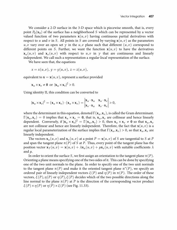
Vector Integration 407
We consider a 2-D surface in the 3-D space which is piecewise smooth, that is, everypoint P0(x0) of the surface has a neighborhood S which can be represented by a vectorvalued function of two parameters x(u,v) having continuous partial derivatives withrespect to u and v in S . All points in S are covered by varying x(u,v) as the parametersu,v vary over an open set γ in the u,v plane such that different (u,v) correspond todifferent points on S . Further, we want the function x(u,v) to have the derivativesxu(u,v) and xv(u,v) with respect to u,v in γ that are continuous and linearlyindependent. We call such a representation a regular local representation of the surface.
We have seen that, the equations
x = x(u,v), y = y(u,v), z = z(u,v),
equivalent to x = x(u,v), represent a surface provided
xu × xv , 0 or |xu × xv|2 > 0.
Using identity II, this condition can be converted to
|xu × xv |2 = (xu × xv) · (xu × xv) =
∣∣∣∣∣∣xu · xu xu · xvxv · xu xv · xv
∣∣∣∣∣∣ > 0,
where the determinant in this equation, denoted Γ (xu ,xv), is called the Gram determinant.Γ (xu ,xv) = 0 implies that xu × xv = 0, that is, xu ,xv are collinear and hence linearlydependent. Conversely, if |xu × xv |2 = Γ (xu ,xv) > 0, then xu × xv , 0 so that xu ,xvare not collinear and hence are linearly independent. Therefore, the fact that x(u,v) is aregular local parameterization of the surface implies that Γ (xu ,xv) > 0, so that xu ,xv arelinearly independent.
The vectors xu(u,v) and xv(u,v) at a point P = x(u,v) of S are tangential to S at Pand span the tangent plane π(P ) of S at P . Thus, every point of the tangent plane has theposition vector xT (u,v) = x(u,v) + λxu(u,v) + µxv(u,v) with suitable coefficients λand µ.
In order to orient the surface S, we first assign an orientation to the tangent planeπ(P ).Orienting a plane means specifying one of the two sides of it. This can be done by specifyingone of the two unit normals to the plane. In order to specify one of the two unit normalsto the tangent plane π(P ) and make it the oriented tangent plane π∗(P ), we specify anordered pair of linearly independent vectors ξ(P ) and η(P ) in π(P ). The order of thesevectors, ξ(P ),η(P ) or η(P ),ξ(P ) decides which of the two possible directions along theline normal to the plane π(P ) at P is the direction of the corresponding vector productξ(P )× η(P ) or η(P )× ξ(P ) (see Fig. 11.33).
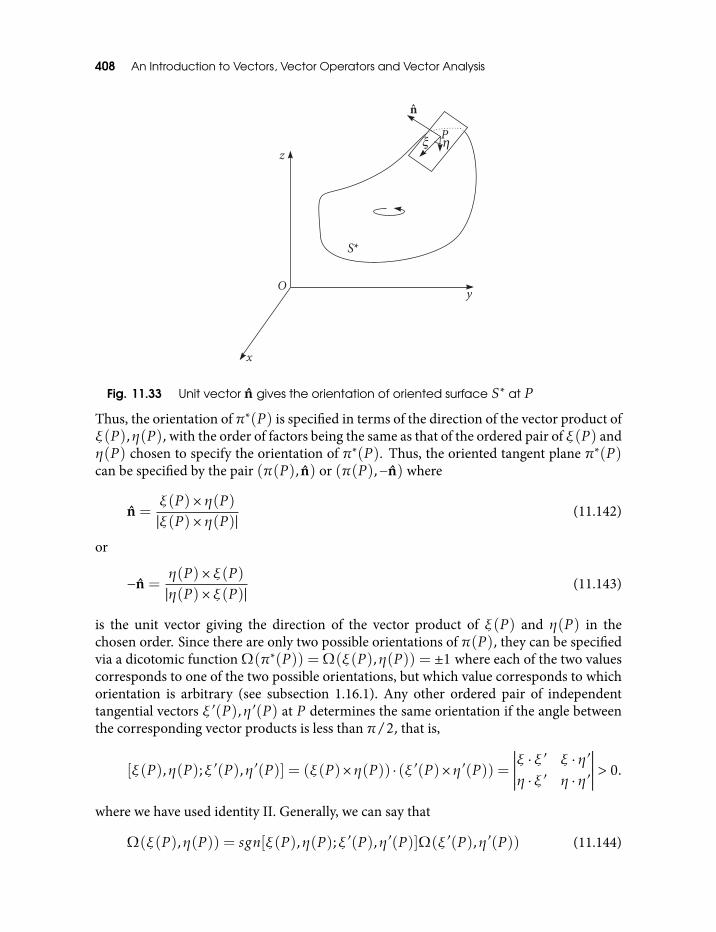
408 An Introduction to Vectors, Vector Operators and Vector Analysis
Fig. 11.33 Unit vector n gives the orientation of oriented surface S∗ at P
Thus, the orientation of π∗(P ) is specified in terms of the direction of the vector product ofξ(P ),η(P ), with the order of factors being the same as that of the ordered pair of ξ(P ) andη(P ) chosen to specify the orientation of π∗(P ). Thus, the oriented tangent plane π∗(P )can be specified by the pair (π(P ), n) or (π(P ),−n) where
n =ξ(P )× η(P )|ξ(P )× η(P )|
(11.142)
or
−n =η(P )× ξ(P )|η(P )× ξ(P )|
(11.143)
is the unit vector giving the direction of the vector product of ξ(P ) and η(P ) in thechosen order. Since there are only two possible orientations of π(P ), they can be specifiedvia a dicotomic function Ω(π∗(P )) =Ω(ξ(P ),η(P )) = ±1 where each of the two valuescorresponds to one of the two possible orientations, but which value corresponds to whichorientation is arbitrary (see subsection 1.16.1). Any other ordered pair of independenttangential vectors ξ ′(P ),η′(P ) at P determines the same orientation if the angle betweenthe corresponding vector products is less than π/2, that is,
[ξ(P ),η(P );ξ ′(P ),η′(P )] = (ξ(P )×η(P )) · (ξ ′(P )×η′(P )) =∣∣∣∣∣∣ξ · ξ ′ ξ · η′
η · ξ ′ η · η′
∣∣∣∣∣∣ > 0.
where we have used identity II. Generally, we can say that
Ω(ξ(P ),η(P )) = sgn[ξ(P ),η(P );ξ ′(P ),η′(P )]Ω(ξ ′(P ),η′(P )) (11.144)
Vector Integration 409
where sgn(x) equals −1 for x < 0 and +1 for x ≥ 0 respectively. Equivalently, the theordered pairs of tangential vectors ξ,η and ξ ′,η′ give the same orientation to π if
n · n′ > 0
where n and n′ are the unit vectors specifying the directions of ξ × η and ξ ′ × η′respectively. Since ξ(P ),η(P ) and ξ ′(P ),η′(P ) belong to the same plane, there are onlytwo possibilities: n · n′ = +1 (n′ = n) or n · n′ = −1 (n′ = −n).
We now use the orientation of the tangent plane to the surface S at a point P on S todefine the orientation of the surface S in the following way. We say that the unit normalsdefining the orientations of the tangent planes π∗(P ) depend continuously on P , whenthese normals to the planes π∗(P ) at the points close to each other (in the Euclideansense) are themselves close to each other (in the Euclidean sense). That is, given ε > 0however small, there exists δ > 0 such that,
√(u −u1)2 + (v − v1)2 < δ implies
|n(x(u,v)) − n(x(u1,v1))| < ε. This is expressed by saying that the the orientationΩ(π∗(P )) of tangent plane at P varies continuously as P varies on S . An oriented surfaceS∗ is defined as a surface S with continuously oriented tangent planes π∗(P ).
It is possible to find another criterion to ascertain the unit vector deciding theorientation of a tangent plane. If ξ,η stands for one of the two ordered pairs drawn outof ξ(P ) and η(P ), then the corresponding unit normal n deciding the orientation ofπ∗(P ) is the one which makes the triplet ξ,η, n positively oriented (see section 1.16).This is equivalent to the following inequality,
n · ξ × η= det(n, ξ,η) = |ξ × η| > 0. (11.145)
Thus, out of the two possible unit vectors perpendicular to π(P ) at P , the unit vectorsatisfying inequality Eq. (11.145) decides the orientation of π(P ). As we show in the nextpara, this vector also specifies the orientation of a connected surface S . Let e1, e2, e3 bethe orthonormal basis to which all vectors are referred. Then, if the triplets (ξ,η, n) ande1, e2, e3, have the same orientation, we can write (see section 1.16),
Ω(ξ,η, n) =Ω(e1, e2, e3)
and we call this vector n, defining the orientation of S∗, the unit normal vector pointing tothe positive side of the oriented surface S∗ or the positive unit normal to S∗.
We can now understand how to assign an orientation to a connected surface S . Wechoose a point P on S, and the pair (ξ,η) in the tangent plane π(P ), which decides, viaEq. (11.142), one of the two possible unit vectors n and n′ specifying the orientation ofS at P . This unit vector actually specifies the orientation of the whole surface S, as thefollowing argument shows. At P we have n′ = εn, where ε = ε(P ) = ±1. Since the unitvectors n, n′ are assumed to vary continuously with P , the same is true for ε(P ) = n · n′ .Thus, ε is a continuous function on S having only the values +1 or −1. If ε(P ) , ε(Q)for any two distinct points P and Q on S, it follows from the continuity of ε that ε = 0at some point along a curve on S joining P and Q, contradicting the definition of ε. As a
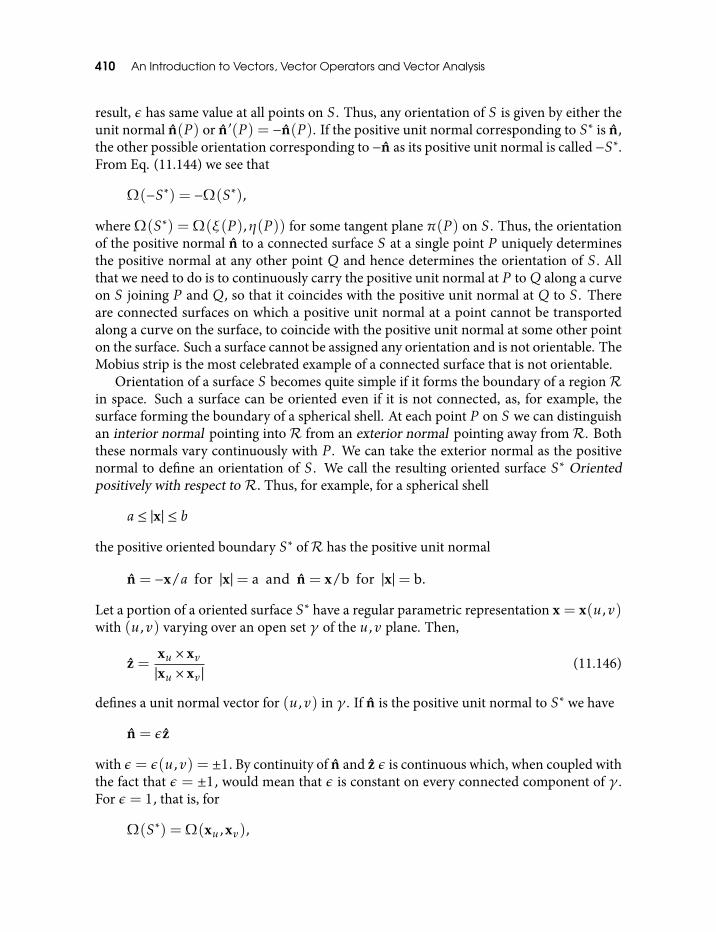
410 An Introduction to Vectors, Vector Operators and Vector Analysis
result, ε has same value at all points on S . Thus, any orientation of S is given by either theunit normal n(P ) or n′(P ) = −n(P ). If the positive unit normal corresponding to S∗ is n,the other possible orientation corresponding to −n as its positive unit normal is called −S∗.From Eq. (11.144) we see that
Ω(−S∗) = −Ω(S∗),
where Ω(S∗) =Ω(ξ(P ),η(P )) for some tangent plane π(P ) on S . Thus, the orientationof the positive normal n to a connected surface S at a single point P uniquely determinesthe positive normal at any other point Q and hence determines the orientation of S . Allthat we need to do is to continuously carry the positive unit normal at P toQ along a curveon S joining P and Q, so that it coincides with the positive unit normal at Q to S . Thereare connected surfaces on which a positive unit normal at a point cannot be transportedalong a curve on the surface, to coincide with the positive unit normal at some other pointon the surface. Such a surface cannot be assigned any orientation and is not orientable. TheMobius strip is the most celebrated example of a connected surface that is not orientable.
Orientation of a surface S becomes quite simple if it forms the boundary of a regionRin space. Such a surface can be oriented even if it is not connected, as, for example, thesurface forming the boundary of a spherical shell. At each point P on S we can distinguishan interior normal pointing intoR from an exterior normal pointing away fromR. Boththese normals vary continuously with P . We can take the exterior normal as the positivenormal to define an orientation of S . We call the resulting oriented surface S∗ Orientedpositively with respect to R. Thus, for example, for a spherical shell
a ≤ |x| ≤ b
the positive oriented boundary S∗ ofR has the positive unit normal
n = −x/a for |x|= a and n = x/b for |x|= b.
Let a portion of a oriented surface S∗ have a regular parametric representation x = x(u,v)with (u,v) varying over an open set γ of the u,v plane. Then,
z =xu × xv|xu × xv |
(11.146)
defines a unit normal vector for (u,v) in γ . If n is the positive unit normal to S∗ we have
n = εz
with ε = ε(u,v) = ±1. By continuity of n and z ε is continuous which, when coupled withthe fact that ε = ±1, would mean that ε is constant on every connected component of γ .For ε = 1, that is, for
Ω(S∗) =Ω(xu ,xv),
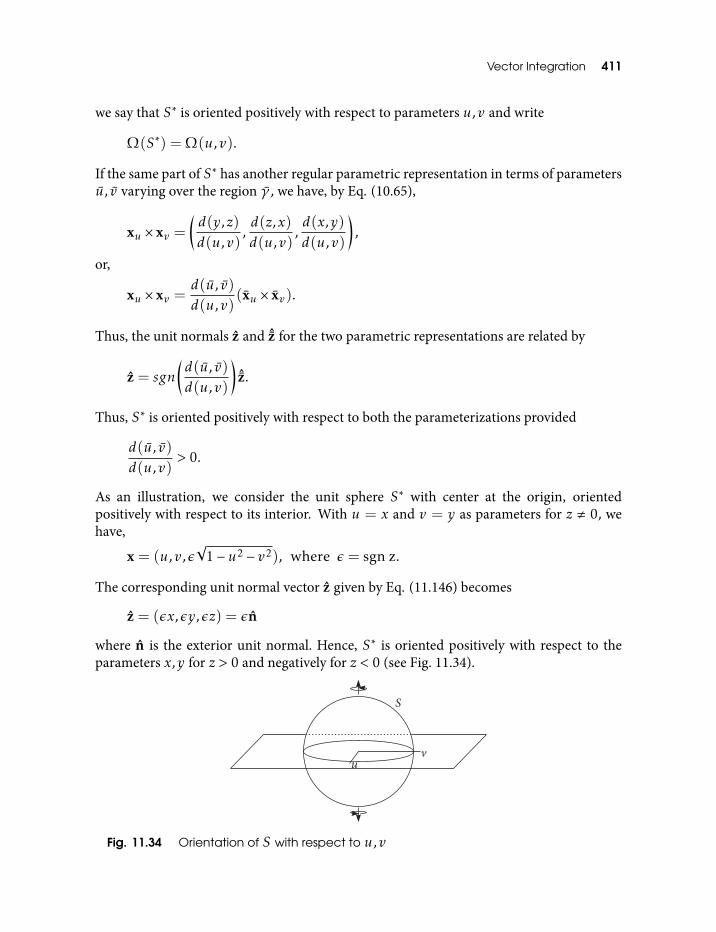
Vector Integration 411
we say that S∗ is oriented positively with respect to parameters u,v and write
Ω(S∗) =Ω(u,v).
If the same part of S∗ has another regular parametric representation in terms of parametersu, v varying over the region γ , we have, by Eq. (10.65),
xu × xv =(d(y,z)d(u,v)
,d(z,x)d(u,v)
,d(x,y)d(u,v)
),
or,
xu × xv =d(u, v)d(u,v)
(xu × xv).
Thus, the unit normals z and ˆz for the two parametric representations are related by
z = sgn
(d(u, v)d(u,v)
)ˆz.
Thus, S∗ is oriented positively with respect to both the parameterizations provided
d(u, v)d(u,v)
> 0.
As an illustration, we consider the unit sphere S∗ with center at the origin, orientedpositively with respect to its interior. With u = x and v = y as parameters for z , 0, wehave,
x = (u,v,ε√
1−u2 − v2), where ε = sgn z.
The corresponding unit normal vector z given by Eq. (11.146) becomes
z = (εx,εy,εz) = εn
where n is the exterior unit normal. Hence, S∗ is oriented positively with respect to theparameters x,y for z > 0 and negatively for z < 0 (see Fig. 11.34).
Fig. 11.34 Orientation of S with respect to u,v
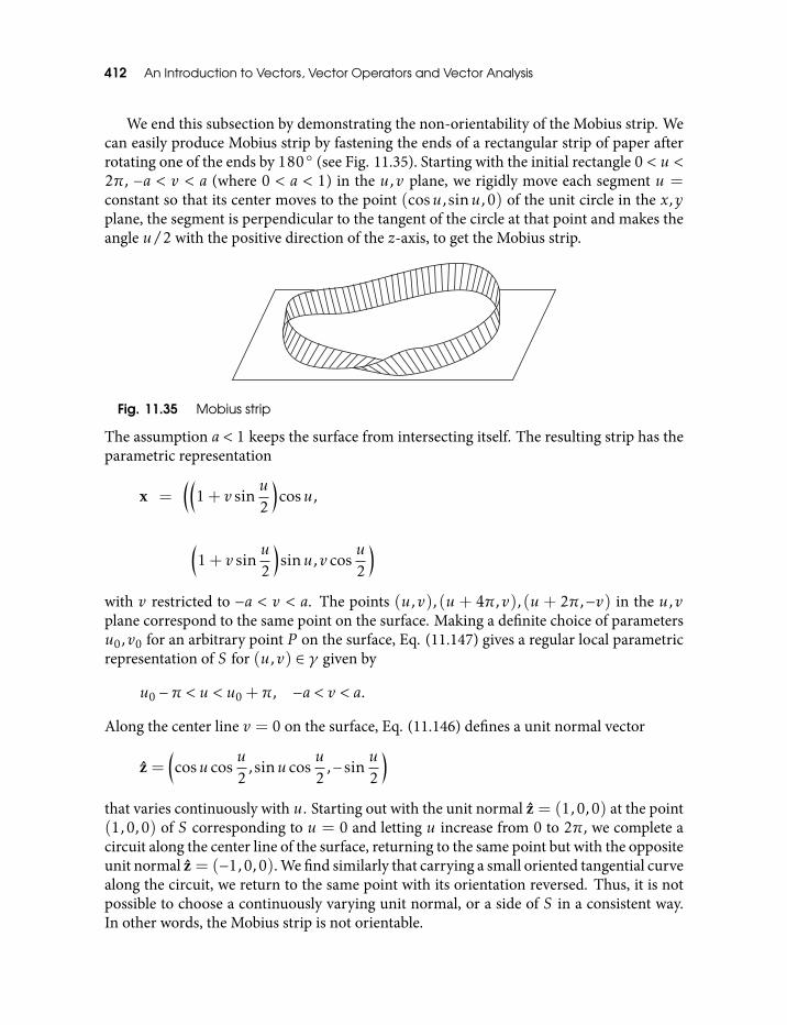
412 An Introduction to Vectors, Vector Operators and Vector Analysis
We end this subsection by demonstrating the non-orientability of the Mobius strip. Wecan easily produce Mobius strip by fastening the ends of a rectangular strip of paper afterrotating one of the ends by 180 (see Fig. 11.35). Starting with the initial rectangle 0 < u <2π, −a < v < a (where 0 < a < 1) in the u,v plane, we rigidly move each segment u =constant so that its center moves to the point (cosu, sinu,0) of the unit circle in the x,yplane, the segment is perpendicular to the tangent of the circle at that point and makes theangle u/2 with the positive direction of the z-axis, to get the Mobius strip.
Fig. 11.35 Mobius strip
The assumption a < 1 keeps the surface from intersecting itself. The resulting strip has theparametric representation
x =((
1+ v sinu2
)cosu,
(1+ v sin
u2
)sinu,v cos
u2
)with v restricted to −a < v < a. The points (u,v), (u + 4π,v), (u + 2π,−v) in the u,vplane correspond to the same point on the surface. Making a definite choice of parametersu0,v0 for an arbitrary point P on the surface, Eq. (11.147) gives a regular local parametricrepresentation of S for (u,v) ∈ γ given by
u0 −π < u < u0 +π, −a < v < a.
Along the center line v = 0 on the surface, Eq. (11.146) defines a unit normal vector
z =(cosu cos
u2
,sinu cosu2
,−sinu2
)that varies continuously with u. Starting out with the unit normal z = (1,0,0) at the point(1,0,0) of S corresponding to u = 0 and letting u increase from 0 to 2π, we complete acircuit along the center line of the surface, returning to the same point but with the oppositeunit normal z = (−1,0,0). We find similarly that carrying a small oriented tangential curvealong the circuit, we return to the same point with its orientation reversed. Thus, it is notpossible to choose a continuously varying unit normal, or a side of S in a consistent way.In other words, the Mobius strip is not orientable.
Vector Integration 413
Exercise Let S be the mobius strip with the parametric representation given byEq. (11.147). (a) Show that the line v = a/2 divides S into an orientable and anon-orientable set. (b) Show that the line v = 0 does not divide S, that is, the set S1obtained by removing all points with v = 0 from S is still connected. (c) Show that S1 isorientable.
Solution
(a) The line v = a/2 divides S into a part S ′ a/2 < v < a (or, equivalently, −a < v <−a/2) and oriented by ξ = xu , η = xv and a part S ′′ given by −a/2 < v < a/2which is just another Mobius strip.
(b) S1 is representable by Ω(ξ(P ),η(P )) with v restricted to the interval 0 < v < a,where P can be varied continuously over S1. Obviously, any two points on S1 can bejoined by a curve on S1 which is the image of the corresponding points (u,v) in theparameter plane.
(c) S1 is oriented by ξ = xu , η = xv .
Exercise Let ξ, η be independent vectors in a plane π. Put a = |ξ |2, b = ξ · η, c = |η|2form for any θ the vector
X(θ) =
(cosθ − b
√ac − b2
sinθ)ξ +
asinθ√ac − b2
η.
Prove that X(θ) is obtained by rotating the vector ξ in the plane π by an angle θ in thesense given by the orientation Ω(ξ,η).
Solution We can easily check that X(θ) has length |ξ | and is linearly dependent on ξ, ηso that X(θ) lies in π. Moreover, X(θ) · ξ/|ξ |2 = cosθ. The vector X(θ) coincides withξ for θ = 0 and has the direction of η for a certain θ between 0 and π, or, for that θdetermined by the relations
cosθ =b√ac
, sinθ =
√1− b
2
ac.
SummaryWe now summarize the relevant points covered in this section. First, an orientable surfaceS has two possible orientations which are given by the two possible normals to the surfaceat some point P on it. These are obtained by choosing two non-collinear (linearlyindependent) vectors ξ and η based at P , spanning the tangent plane to S at P . We formtwo possible ordered pairs (ξ,η) and (η,ξ) to define two possible unit normals to thetangent plane or to the surface S at P :
n =ξ × η|ξ × η|
; −n =η × ξ|η × ξ |
.
414 An Introduction to Vectors, Vector Operators and Vector Analysis
We denote the corresponding oriented surface by S∗. From the above equations it is clearthat the triplet (ξ,η, n) is positively oriented, while the triplet (ξ,η,−n) is negativelyoriented. In order to decide which of these unit normals define the positive orientation ofS∗, we first orient the 3-D space containing S∗ as follows. We choose a coordinate systemdefined by the orthonormal basis (e1, e2, e3) to resolve the vectors in some region of spaceR and say that R is positively oriented if this coordinate system is right handed andnegatively oriented if it is left handed. If the coordinate system is right handed, it has thesame orientation as the triplet (ξ,η, n) and we say that n defines the positive orientationof S∗ and −n defines its negative orientation. On the other hand, if the coordinate systemis left handed, it has the same orientation as (ξ,η,−n) and we say that −n defines thepositive orientation of S∗ and n defines its negative orientation. In general, a unit vector ndefining the positive orientation of S∗ is said to be on the positive side of S∗. For a closedsurface S at the boundary of a region R we choose the coordinate system such that theunit normal defining the positive orientation of S∗ is its outward normal.
If a surface S is parameterized by a C1 function x = x(u,v), we can replace the pair(ξ,η) by the pair of tangent vectors (xu ,xv) to define the unit vector, via their vectorproduct, giving the orientation of S∗. If this unit vector z defines the positive orientation ofS∗, we say that S∗ is positively oriented with respect to the parameters u,v.
Now, consider an oriented surface S∗ with an oriented and closed boundary curve C∗.Let the unit normal vector n at point P on S decide the orientation of S∗. We drop aperpendicular from P to the plane containing the curve C∗ to meet this plane at point O.Let P1 and P2 be the points on C∗ such that traversing C∗ from P1 toward P2 is in the samesense defining the orientation of C∗. Then C∗ is positively oriented with respect to S∗ if thetriplet (
−−→OP 1,
−−→OP 2, n) is positively oriented. Further, we say that S∗ is positively oriented
with respect to the x,y axes if the triplet (e1, e2, n) is positively oriented.
11.8 Surface IntegralsThe orientation of the region over which an integral is carried out is fundamentallyconnected to its value, although the Riemannian sums involved are defined in terms ofquantities like length, area and volume, which are inherently positive quantities. Thus, ifwe want the additivity rule∫ b
af (x)dx+
∫ c
bf (x)dx =
∫ c
af (x)dx
to hold without restricting the relative positions of a,b,c, we have to define∫ baf (x)dx both
for a ≤ b as well as a ≥ b by the relation∫ b
af (x)dx = −
∫ a
bf (x)dx. (11.147)
Vector Integration 415
Geometrically, the ordered pair of numbers a,b determines an oriented interval I ∗ on thex-axis with initial point a and the final point b. The value of∫ b
af (x)dx =
∫I∗f (x)dx
is the one given by the limit of the Riemann sum (positive for positive f ) when theorientation of I ∗ corresponds to the sense of increasing x, that is, for a < b. Interchangingthe end points of I ∗ converts I ∗ into the interval −I ∗, with opposite orientation, so thatEq. (11.147) can also be written as∫
−I∗f (x)dx = −
∫I∗f (x)dx. (11.148)
A similar situation prevails regarding the integral over an oriented region R∗ in the x,yplane. When R∗ is oriented positively with respect to the e1, e2 basis defining thecoordinate system, Ω(R∗) = Ω(e1, e2), the differential area dxdy is positive and thedouble integral∫ ∫
R∗f (x,y)dxdy
is the limit of the Riemann sums obtained from the subdivisions of the plane into squaresof area 2−2n. The integral has a non-negative value for a non-negative f . In case Ω(R∗) =−Ω(e1, e2) =Ω(e2, e1) resulting in a negative value for the differential area dydx we get∫ ∫
R∗f dxdy = −
∫ ∫R∗f dydx,
where the integral on the right has the usual meaning as the limit of sums. Thus, we havethe rule that∫ ∫
−R∗f dxdy = −
∫ ∫R∗f dxdy,
where −R∗ is obtained by changing the orientation of R∗. The substitution formula givenby Eq. (11.99) becomes, for the oriented regionR∗,∫ ∫
R∗f (x,y)dxdy =
∫ ∫T ∗f (x(u,v),y(u,v))
d(x,y)d(u,v)
dudv,
for smooth 1− 1 mappings
x = x(u,v), y = y(u,v)
416 An Introduction to Vectors, Vector Operators and Vector Analysis
of T ∗ onto R∗ as long as the Jacobian determinant d(x,y)/d(u,v) has the same signthroughout T ∗. The sign given by the orientation ofR∗ or that of T ∗ to the correspondingintegrals is determined as follows. The rule is that the orientation of R∗ attributes apositive sign to dxdy if the x,y coordinate system has the orientation of R∗ and negativeone otherwise. The sign attributed by the orientation of T ∗ to dudv is then the one thatagrees with the relation
dxdy =d(x,y)d(u,v)
dudv.
Once the proper sign is attached to the differential area dS = dxdy or dT = dudv, therest of the integration amounts to the evaluation of the corresponding double integral.
While learning about line integrals, we came across linear differential forms, alsocalled first order differential forms, which are expressions linear in the differentialsdx,dy,dz. A second order differential form is an expression quadratic in the differentialsdx,dy,dz and has the form
ω = a(x)dxdy+ b(x)dydz+ c(x)dzdx
where a,b,c are C1 functions over their domain. Here, we obtain a general form of thesurface integral of the second order differential form over an oriented surface S∗ in termsof the surface integral of functions over the unoriented surface S . We already know that ifS has the parametric representation
x = x(u,v), y = y(u,v), z = z(u,v)
and if ξ,η,ζ denote the components of the normal vector
ξ =d(y,z)d(u,v)
, η =d(z,x)d(u,v)
, ζ =d(x,y)d(u,v)
, (11.149)
the area of S is given by
A=
∫ ∫R
√ξ2 + η2 + ζ2dudv.
Here, the integral is over the regionR in the u,v plane corresponding to S The integral isunderstood in the sense of a double integral with the surface element
dS =√ξ2 + η2 + ζ2dudv
being treated as a positive quantity or, equivalently,R is given the positive orientation withrespect to the u,v system. Orientability of S is not essential for the definition of A.
Exercise Express the total area of the Mobius strip as an integral, using its parametricrepresentation given by Eq. (11.147).
Vector Integration 417
More generally, for a function f (x) defined on the surface S, we can form the integral of fover the surface:∫ ∫
Sf dS =
∫ ∫Rf
√ξ2 + η2 + ζ2dudv. (11.150)
The value of this integral is independent of the particular parametric representation usedfor S and does not involve any orientation of S . It is positive for positive f .
In order to relate the integral of a second order differential form over an orientedsurface S∗ to the surface integrals of functions over the unoriented surface S as defined byEq. (11.150), we introduce the direction cosines of the positive normal to S∗
cosα =εξ√
ξ2 + η2 + ζ2, cosβ =
εη√ξ2 + η2 + ζ2
, cosγ =εζ√
ξ2 + η2 + ζ2,
where ξ,η,ζ are as defined in Eq. (11.149), ε = ±1 and Ω(S∗) = εΩ(xu ,xv) (seesubsection 1.16.1). We can write ω in the form
ω = Kdudv
where
K =ω
dudv= a
d(y,z)d(u,v)
+ bd(z,x)d(u,v)
+ cd(x,y)d(u,v)
(11.151)
so that∫ ∫S∗ω =
∫ ∫R∗Kdudv
=
∫ ∫R∗
(ad(y,z)d(u,v)
+ bd(z,x)d(u,v)
+ cd(x,y)d(u,v)
)dudv. (11.152)
Exercise Show that the value of this integral of ω over the oriented surface S∗ isindependent of the particular parametric representation for S∗.
From Eqs (11.151) and (11.152) we can write
K =ω
dudv= ε(acosα+ bcosβ+ ccosγ)
√ξ2 + η2 + ζ2.
By Eq. (11.152)∫ ∫S∗ω =
∫ ∫R∗Kdudv = ε
∫ ∫RKdudv.
418 An Introduction to Vectors, Vector Operators and Vector Analysis
Therefore, Eq. (11.150) yields the identity∫ ∫S∗ω =
∫ ∫S∗adydz+ bdzdx+ cdxdy
=
∫ ∫S(acosα+ bcosβ+ ccosγ)dS
=
∫ ∫R(acosα+ bcosβ+ ccosγ)
√ξ2 + η2 + ζ2dudv, (11.153)
which expresses the integral of the differential form ω over the oriented surface S∗ as anintegral over the unoriented surface S or over the unoriented region R in the parameterplane. Note, however, that here the integrand depends on the orientation of S∗, since itinvolves the direction cosines of the normal n to S∗ pointing to its positive side. If theoriented surface S∗ comprises many parts S∗i each having a parametric representation x =x(u,v) we apply identity Eq. (11.153) to each part and add over different parts to get thesame identity for the integral of ω over the whole surface S∗.
The direction cosines of the normal n pointing to the positive side of S∗ can be identifiedwith the derivatives of x,y,z in the direction of n, so that4∫ ∫
S∗ω =
∫ ∫S
(adxdn
+ bdy
dn+ c
dzdn
)dS (11.154)
or, in vector notation∫ ∫S∗ω =
∫ ∫S
v · ndS, (11.155)
where n ≡ (cosα, cosβ, cosγ) is the unit normal vector on the positive side of S∗ and v(x)is the vector field with components (a(x),b(x),c(x)).
The concept of a surface integral can be interpreted in terms of the 3-D flow of anincompressible fluid of unit density. Let the vector field v(x) be the velocity field of thisflow. Then at each point of the surface S∗ the product v · n gives the component of thevelocity of the flow in the direction of the normal n to the surface. The expression v · ndScan then be identified with the amount of fluid that flows across the element of surface dSfrom the negative side of S∗ to the positive side in unit time. Note that this quantity may benegative. The surface integral in Eq. (11.155) therefore represents the total amount of fluidflowing across the surface S∗ from the negative to the positive side in unit time. Note thefundamental part played by the orientation (distinction between the positive and negativesides) of S∗ in the description of the motion of the fluid.
We may also consider the field defined by the integrand of Eq. (11.155) as the field offorce F(x). The direction of the vector F then gives the direction of the lines of force and its
4We have, dxdn = n · ∇x = [cosα cosβ cosγ ][1 0 0]T = cosα etc.
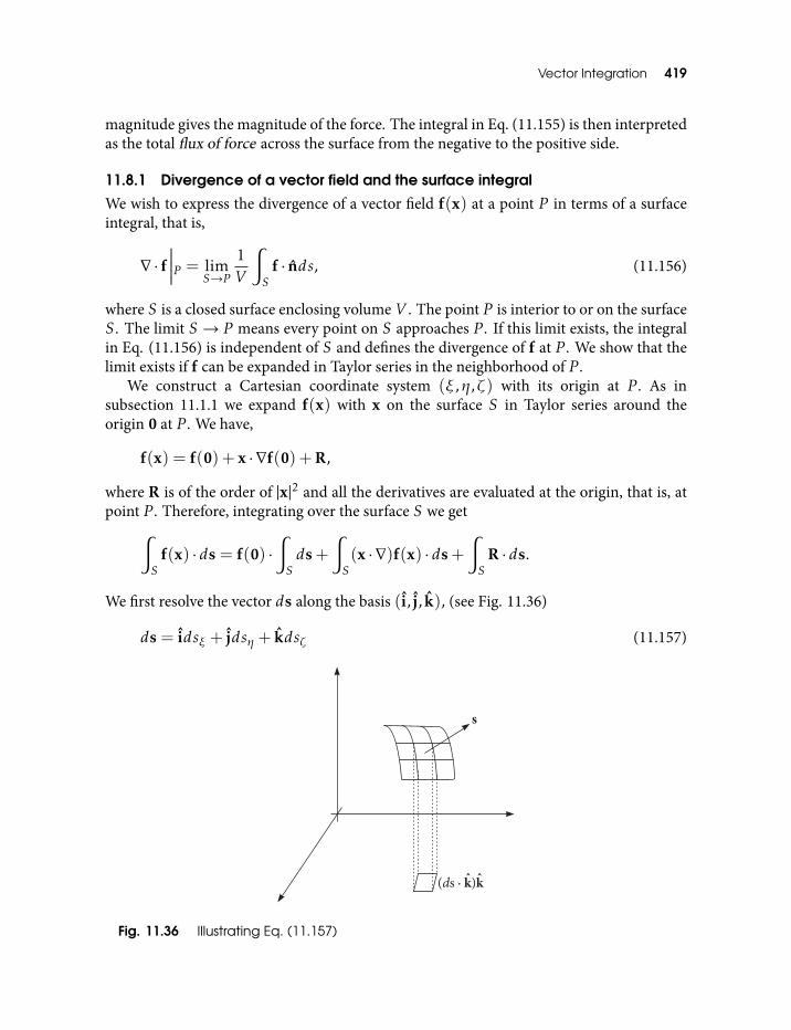
Vector Integration 419
magnitude gives the magnitude of the force. The integral in Eq. (11.155) is then interpretedas the total flux of force across the surface from the negative to the positive side.
11.8.1 Divergence of a vector field and the surface integral
We wish to express the divergence of a vector field f(x) at a point P in terms of a surfaceintegral, that is,
∇ · f∣∣∣∣∣P = lim
S→P
1V
∫S
f · nds, (11.156)
where S is a closed surface enclosing volume V . The point P is interior to or on the surfaceS . The limit S → P means every point on S approaches P . If this limit exists, the integralin Eq. (11.156) is independent of S and defines the divergence of f at P . We show that thelimit exists if f can be expanded in Taylor series in the neighborhood of P .
We construct a Cartesian coordinate system (ξ,η,ζ) with its origin at P . As insubsection 11.1.1 we expand f(x) with x on the surface S in Taylor series around theorigin 0 at P . We have,
f(x) = f(0) + x · ∇f(0) +R,
where R is of the order of |x|2 and all the derivatives are evaluated at the origin, that is, atpoint P . Therefore, integrating over the surface S we get∫
Sf(x) · ds = f(0) ·
∫Sds+
∫S(x · ∇)f(x) · ds+
∫S
R · ds.
We first resolve the vector ds along the basis (i, j, k), (see Fig. 11.36)
ds = idsξ + jdsη + kdsζ (11.157)
Fig. 11.36 Illustrating Eq. (11.157)
420 An Introduction to Vectors, Vector Operators and Vector Analysis
where the components of ds are the projections of ds on yz,zx and xy planes respectively.As in subsection 11.1.1 we express (x · ∇)f(x) · ds in terms of the derivatives with respectto (ξ,η,ζ) to get∫
Sf · ds = f(0) ·
∫Sds+
∂fξ∂ξ
∫Sξ
ξdsξ +∂fξ∂η
∫Sξ
ηdsξ +∂fξ∂ζ
∫Sξ
ζdsξ
∂fη∂ξ
∫Sη
ξdsη +∂fη∂η
∫Sη
ηdsη +∂fη∂ζ
∫Sη
ζdsη
∂fζ∂ξ
∫Sζ
ξdsζ +∂fζ∂η
∫Sζ
ηdsζ +∂fζ∂ζ
∫Sζ
ζdsζ +
∫S
R · ds,
where (Sξ ,Sη ,Sζ) are the projections of S on the coordinate planes and the last integralgoes as |x|4. We shall show later in an exercise that∫
Sds = 0.
Further,∫Sξ
ξdsξ = V ,
since∫Sξξdsξ gives the volume under the upper part minus that under the lower part (see
subsection 11.4.2). Similarly,∫Sη
ηdsη = V =
∫Sζ
ζdsζ .
Moreover, the integrals of the form∫Sξηdsξ vanish. Everything put together we get∫
Sf · ds =
(∂fξ∂ξ
+∂fη∂η
+∂fζ∂ζ
)V +O(|x|4).
Divide both sides by V , (so that the last term is O(|x|) and goes to zero as |x| → 0), andtake the limit as |x| → 0 to get
limS→P
1V
∫S
f · ds =(∂fξ∂ξ
+∂fη∂η
+∂fζ∂ζ
)= ∇ · f.
Thus, the limit exists and does not depend on S . It depends only on the derivatives of f atpoint P .
Vector Integration 421
Exercise Let S be a closed surface and let P be an interior point of S or a point on S . Fora scalar field f and a vector field F show that
∇f = limS→P
1V
∫Sf ds
and
∇×F = limS→P
1V
∫Sds×F.
11.9 Diveregence Theorem in Three-dimensionsThis is the extension of the Gauss’s theorem in two dimensions we proved before. There anintegral over a plane region is reduced to a line integral taken around the boundary of theregion. In its 3-D version, we consider a closed bounded region R in space bounded bya surface S . To start with we assume that S is intersected by every straight line parallel tox,y,z axes only at two points, or does not intersect at all. We will remove this assumptionlater. Let the functions a(x),b(x),c(x) be C1 inR. Consider the integral∫ ∫ ∫
R
∂c∂zdxdydz
over the regionR, oriented positively with respect to x,y,z coordinate system. Due to theassumption made regarding the mesh of straight lines parallel to the axes and the regionR,such a regionR can be described by the inequalities
z0(x,y) ≤ z ≤ z1(x,y)
where (x,y) varies over the projection B of R on the x,y plane. We assume that B has anarea and that the functions z0(x,y) and z1(x,y) are C1 in B. We can express the volumeintegral overR as the succession of integrals∫ ∫ ∫
Rf dxdydz =
∫ ∫Bdxdy
∫ z1
z0
f dz.
Here, f = ∂c/∂z so that the integral over z can be carried out, giving∫ z1
z0
∂c∂z
= c(x,y,z1)− c(x,y,z0) = c1 − c0,
so that,∫ ∫ ∫R
∂c∂zdxdydz =
∫ ∫Bc1dxdy −
∫ ∫Bc0dxdy.
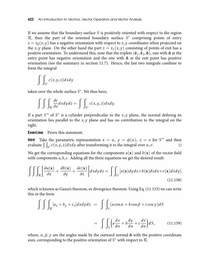
422 An Introduction to Vectors, Vector Operators and Vector Analysis
If we assume that the boundary surface S is positively oriented with respect to the regionR, then the part of the oriented boundary surface S∗ comprising points of entryz = z0(x,y) has a negative orientation with respect to x,y coordinates when projected onthe x,y plane. On the other hand the part z = z1(x,y) consisting of points of exit has apositive orientation. To understand this, note that the triplets (e1, e2, n), one with n at theentry point has negative orientation and the one with n at the exit point has positiveorientation (see the summary in section 11.7). Hence, the last two integrals combine toform the integral∫ ∫
S∗c(x,y,z)dxdy
taken over the whole surface S∗. We thus have,∫ ∫ ∫R
∂c∂zdxdydz =
∫ ∫S∗c(x,y,z)dxdy.
If a part S ′∗ of S∗ is a cylinder perpendicular to the x,y plane, the normal defining itsorientation lies parallel to the x,y plane and has no contribution to the integral on theright.
Exercise Prove this statement.
Hint Take the parametric representation x = u, y = φ(u), z = v for S ′∗ and thenevaluate
∫ ∫S∗c(x,y,z)dxdy after transforming it to the integral over u,v.
We get the corresponding equations for the components a(x) and b(x) of the vector fieldwith components a,b,c. Adding all the three equations we get the desired result:∫ ∫ ∫
R
[∂a(x)∂x
+∂b(x)∂y
+∂c(x)∂z
]dxdydz =
∫ ∫S∗[a(x)dydz+b(x)dzdx+c(x)dxdy].
(11.158)
which is known as Gauss’s theorem, or divergence theorem. Using Eq. (11.153) we can writethis in the form∫ ∫ ∫
R[ax+ by + cz]dxdydz =
∫ ∫S(acosα+ bcosβ+ ccosγ)dS
=
∫ ∫S
(adxdn
+ bdy
dn+ c
dzdn
)dS, (11.159)
where, α,β,γ are the angles made by the outward normal n with the positive coordinateaxes, corresponding to the positive orientation of S∗ with respect toR.
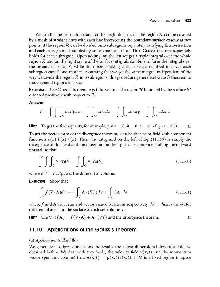
Vector Integration 423
We can lift the restriction stated at the beginning, that is the region R can be coveredby a mesh of straight lines with each line intersecting the boundary surface exactly at twopoints, if the regionR can be divided onto subregions separately satisfying this restrictionand each subregion is bounded by an orientable surface. Then Gauss’s theorem separatelyholds for each subregion. Upon adding, on the left we get a triple integral over the wholeregion R and on the right some of the surface integrals combine to form the integral overthe oriented surface S, while the others making extra surfaces required to cover eachsubregion cancel one another. Assuming that we get the same integral independent of theway we divide the regionR into subregions, this procedure generalizes Gauss’s theorem tomore general regions in space.Exercise Use Gauss’s theorem to get the volume of a regionR bounded by the surface S∗oriented positively with respect toR.
Answer
V =
∫ ∫ ∫Rdxdydz =
∫ ∫S∗xdydz =
∫ ∫S∗zdxdy =
∫ ∫S∗ydzdx.
Hint To get the first equality, for example, put a= 0, b = 0, c = z in Eq. (11.158).
To get the vector form of the divergence theorem, let v be the vector field with componentfunctions a(x),b(x),c(x). Then, the integrand on the left of Eq. (11.159) is simply thedivergence of this field and the integrand on the right is its component along the outwardnormal, so that∫ ∫ ∫
R∇ · vdV =
∫ ∫S∗
v · ndS, (11.160)
where dV = dxdydz is the differential volume.
Exercise Show that∫Vf (∇ ·A)dτ = −
∫V
A · (∇f )dτ +∫Sf A · da (11.161)
where f and A are scalar and vector valued functions respectively, da = dan is the vectordifferential area and the surface S encloses volume V .
Hint Use ∇ · (f A) = f (∇ ·A) +A · (∇f ) and the divergence theorem.
11.10 Applications of the Gauss’s Theorem
(a) Application to fluid flowWe generalize to three dimensions the results about two dimensional flow of a fluid weobtained before. We deal with two fields, the velocity field v(x, t) and the momentumvector (per unit volume) field A(x, t) = ρ(x, t)v(x, t). If R is a fixed region in space
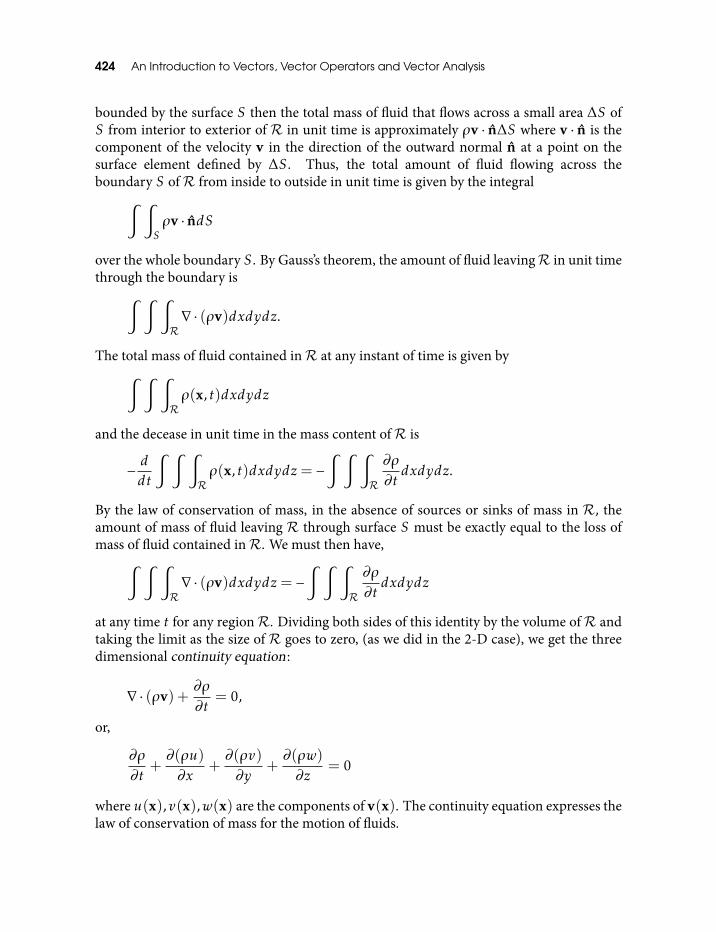
424 An Introduction to Vectors, Vector Operators and Vector Analysis
bounded by the surface S then the total mass of fluid that flows across a small area ∆S ofS from interior to exterior of R in unit time is approximately ρv · n∆S where v · n is thecomponent of the velocity v in the direction of the outward normal n at a point on thesurface element defined by ∆S . Thus, the total amount of fluid flowing across theboundary S ofR from inside to outside in unit time is given by the integral∫ ∫
Sρv · ndS
over the whole boundary S . By Gauss’s theorem, the amount of fluid leavingR in unit timethrough the boundary is∫ ∫ ∫
R∇ · (ρv)dxdydz.
The total mass of fluid contained inR at any instant of time is given by∫ ∫ ∫Rρ(x, t)dxdydz
and the decease in unit time in the mass content ofR is
− ddt
∫ ∫ ∫Rρ(x, t)dxdydz = −
∫ ∫ ∫R
∂ρ
∂tdxdydz.
By the law of conservation of mass, in the absence of sources or sinks of mass in R, theamount of mass of fluid leaving R through surface S must be exactly equal to the loss ofmass of fluid contained inR. We must then have,∫ ∫ ∫
R∇ · (ρv)dxdydz = −
∫ ∫ ∫R
∂ρ
∂tdxdydz
at any time t for any regionR. Dividing both sides of this identity by the volume ofR andtaking the limit as the size of R goes to zero, (as we did in the 2-D case), we get the threedimensional continuity equation :
∇ · (ρv) +∂ρ
∂t= 0,
or,
∂ρ
∂t+∂(ρu)
∂x+∂(ρv)
∂y+∂(ρw)
∂z= 0
where u(x),v(x),w(x) are the components of v(x). The continuity equation expresses thelaw of conservation of mass for the motion of fluids.
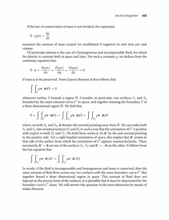
Vector Integration 425
If the law of conservation of mass is not invoked, the expression
∇ · (ρv) +∂ρ
∂t
measures the amount of mass created (or annihilated if negative) in unit time per unitvolume.
Of particular interest is the case of a homogeneous and incompressible fluid, for whichthe density is constant both in space and time. For such a constant ρ, we deduce from thecontinuity equation that,
∇ · v =∂(ρu)
∂x+∂(ρv)
∂y+∂(ρw)
∂z= 0
if mass is to be preserved. From Gauss’s theorem it then follows that∫ ∫Sρv · ndS = 0
whenever surface S bounds a region R. Consider, in particular, two surfaces S1 and S2bounded by the same oriented curve C∗ in space, and together forming the boundary S ofa three dimensional regionR. We find that
0 =
∫ ∫Sρv · ndS =
∫ ∫S1
ρv · ndS +∫ ∫
S2
ρv · ndS
where, on both S1 and S2, n denotes the normal pointing away fromR. We can make bothS1 and S2 into oriented surfaces S∗1 and S∗2 in such a way that the orientation of C∗ is positivewith respect to both S∗1 and S∗2. On both these surfaces, let n∗ be the unit normal pointingto the positive side. For a right handed orientation of space, this implies that n∗ points tothat side of the surface from which the orientation of C∗ appears counterclockwise. Then,necessarily, n∗ = n on one of the surfaces S1, S2 and n∗ = −n on the other. It follows fromthe last equation that∫ ∫
S1
ρv · n∗dS =
∫ ∫S2
ρv · n∗dS.
In words, if the fluid is incompressible and homogeneous and mass is conserved, then thesame amount of fluid flows across any two surfaces with the same boundary curve C∗ thattogether bound a three dimensional region in space. This amount of fluid does notdepend on the precise form of the surfaces, it is plausible that it must be determined by theboundary curve C∗ alone. We will answer this question in the next subsection by means ofstokes theorem.
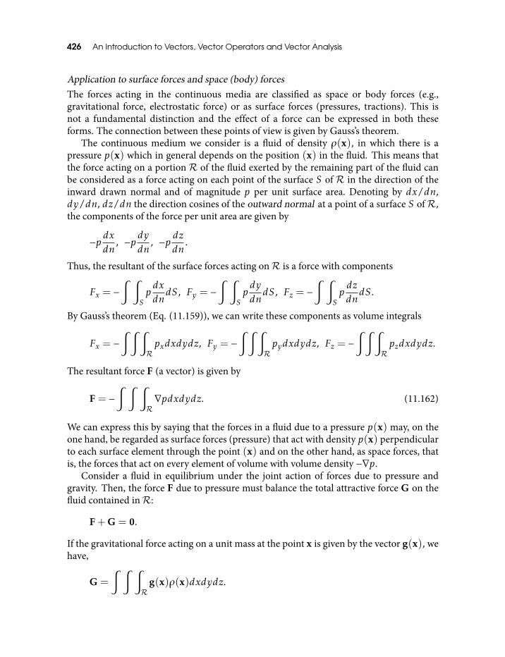
426 An Introduction to Vectors, Vector Operators and Vector Analysis
Application to surface forces and space (body) forcesThe forces acting in the continuous media are classified as space or body forces (e.g.,gravitational force, electrostatic force) or as surface forces (pressures, tractions). This isnot a fundamental distinction and the effect of a force can be expressed in both theseforms. The connection between these points of view is given by Gauss’s theorem.
The continuous medium we consider is a fluid of density ρ(x), in which there is apressure p(x) which in general depends on the position (x) in the fluid. This means thatthe force acting on a portion R of the fluid exerted by the remaining part of the fluid canbe considered as a force acting on each point of the surface S of R in the direction of theinward drawn normal and of magnitude p per unit surface area. Denoting by dx/dn,dy/dn, dz/dn the direction cosines of the outward normal at a point of a surface S ofR,the components of the force per unit area are given by
−pdxdn
, −pdy
dn, −p dz
dn.
Thus, the resultant of the surface forces acting onR is a force with components
Fx = −∫ ∫
SpdxdndS, Fy = −
∫ ∫Spdy
dndS, Fz = −
∫ ∫SpdzdndS.
By Gauss’s theorem (Eq. (11.159)), we can write these components as volume integrals
Fx = −∫ ∫ ∫
Rpxdxdydz, Fy = −
∫ ∫ ∫Rpydxdydz, Fz = −
∫ ∫ ∫Rpzdxdydz.
The resultant force F (a vector) is given by
F = −∫ ∫ ∫
R∇pdxdydz. (11.162)
We can express this by saying that the forces in a fluid due to a pressure p(x) may, on theone hand, be regarded as surface forces (pressure) that act with density p(x) perpendicularto each surface element through the point (x) and on the other hand, as space forces, thatis, the forces that act on every element of volume with volume density −∇p.
Consider a fluid in equilibrium under the joint action of forces due to pressure andgravity. Then, the force F due to pressure must balance the total attractive force G on thefluid contained inR:
F+G = 0.
If the gravitational force acting on a unit mass at the point x is given by the vector g(x), wehave,
G =
∫ ∫ ∫R
g(x)ρ(x)dxdydz.
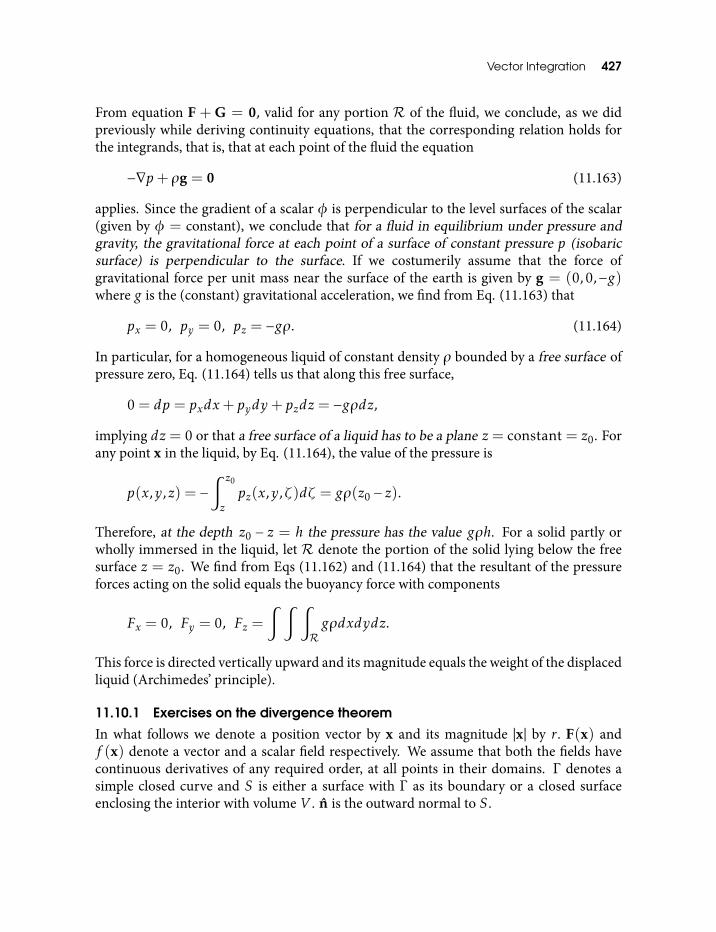
Vector Integration 427
From equation F + G = 0, valid for any portion R of the fluid, we conclude, as we didpreviously while deriving continuity equations, that the corresponding relation holds forthe integrands, that is, that at each point of the fluid the equation
−∇p+ ρg = 0 (11.163)
applies. Since the gradient of a scalar φ is perpendicular to the level surfaces of the scalar(given by φ = constant), we conclude that for a fluid in equilibrium under pressure andgravity, the gravitational force at each point of a surface of constant pressure p (isobaricsurface) is perpendicular to the surface. If we costumerily assume that the force ofgravitational force per unit mass near the surface of the earth is given by g = (0,0,−g)where g is the (constant) gravitational acceleration, we find from Eq. (11.163) that
px = 0, py = 0, pz = −gρ. (11.164)
In particular, for a homogeneous liquid of constant density ρ bounded by a free surface ofpressure zero, Eq. (11.164) tells us that along this free surface,
0 = dp = pxdx+ pydy+ pzdz = −gρdz,
implying dz = 0 or that a free surface of a liquid has to be a plane z = constant = z0. Forany point x in the liquid, by Eq. (11.164), the value of the pressure is
p(x,y,z) = −∫ z0
zpz(x,y,ζ)dζ = gρ(z0 − z).
Therefore, at the depth z0 − z = h the pressure has the value gρh. For a solid partly orwholly immersed in the liquid, let R denote the portion of the solid lying below the freesurface z = z0. We find from Eqs (11.162) and (11.164) that the resultant of the pressureforces acting on the solid equals the buoyancy force with components
Fx = 0, Fy = 0, Fz =∫ ∫ ∫
Rgρdxdydz.
This force is directed vertically upward and its magnitude equals the weight of the displacedliquid (Archimedes’ principle).
11.10.1 Exercises on the divergence theorem
In what follows we denote a position vector by x and its magnitude |x| by r . F(x) andf (x) denote a vector and a scalar field respectively. We assume that both the fields havecontinuous derivatives of any required order, at all points in their domains. Γ denotes asimple closed curve and S is either a surface with Γ as its boundary or a closed surfaceenclosing the interior with volume V . n is the outward normal to S .
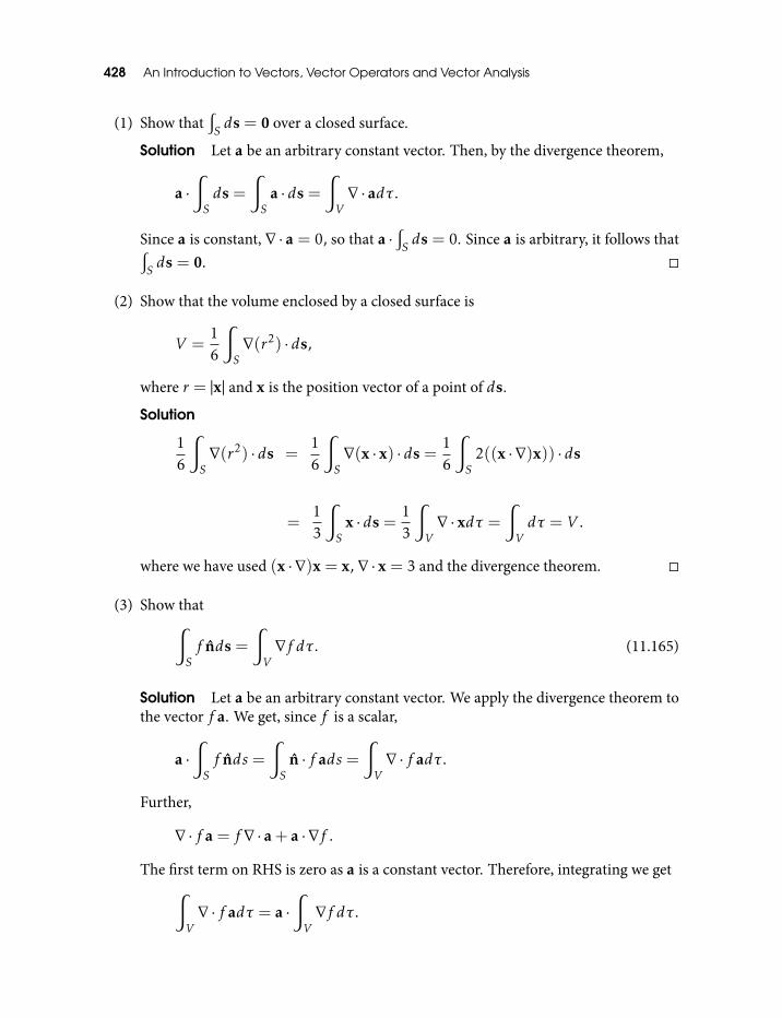
428 An Introduction to Vectors, Vector Operators and Vector Analysis
(1) Show that∫Sds = 0 over a closed surface.
Solution Let a be an arbitrary constant vector. Then, by the divergence theorem,
a ·∫Sds =
∫S
a · ds =∫V∇ · adτ .
Since a is constant, ∇ · a = 0, so that a ·∫Sds = 0. Since a is arbitrary, it follows that∫
Sds = 0.
(2) Show that the volume enclosed by a closed surface is
V =16
∫S∇(r2) · ds,
where r = |x| and x is the position vector of a point of ds.
Solution
16
∫S∇(r2) · ds =
16
∫S∇(x · x) · ds =
16
∫S
2((x · ∇)x)) · ds
=13
∫S
x · ds =13
∫V∇ · xdτ =
∫Vdτ = V .
where we have used (x · ∇)x = x, ∇ · x = 3 and the divergence theorem.
(3) Show that∫Sf nds =
∫V∇f dτ . (11.165)
Solution Let a be an arbitrary constant vector. We apply the divergence theorem tothe vector f a. We get, since f is a scalar,
a ·∫Sf nds =
∫S
n · f ads =∫V∇ · f adτ .
Further,
∇ · f a = f ∇ · a+ a · ∇f .
The first term on RHS is zero as a is a constant vector. Therefore, integrating we get∫V∇ · f adτ = a ·
∫V∇f dτ .
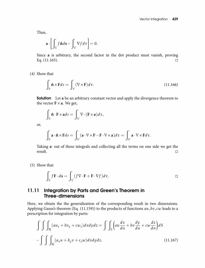
Vector Integration 429
Thus,
a ·[∫
Sf nds−
∫V∇f dτ
]= 0.
Since a is arbitrary, the second factor in the dot product must vanish, provingEq. (11.165).
(4) Show that∫S
n×Fds =∫V(∇×F)dτ . (11.166)
Solution Let a be an arbitrary constant vector and apply the divergence theorem tothe vector F× a. We get,∫
Sn ·F× ads =
∫V∇ · (F× a)dτ ,
or, ∫S
a · n×Fds =∫V(a · ∇ ×F−F · ∇ × a)dτ =
∫V
a · ∇ ×Fdτ .
Taking a· out of these integrals and collecting all the terms on one side we get theresult.
(5) Show that∫Sf F · ds =
∫V(f ∇ ·F+ F · ∇f )dτ .
11.11 Integration by Parts and Green’s Theorem inThree-dimensions
Here, we obtain the the generalization of the corresponding result in two dimensions.Applying Gauss’s theorem (Eq. (11.159)) to the products of functions au,bv,cw leads to aprescription for integration by parts:∫ ∫ ∫
R(aux+ bvy + cwz)dxdydz =
∫ ∫S
(audxdn
+ bvdy
dn+ cw
dzdn
)dS
−∫ ∫ ∫
R(axu+ byv+ czw)dxdydz. (11.167)
430 An Introduction to Vectors, Vector Operators and Vector Analysis
If u = v = w = U and if a,b,c are of the form a = Vx,b = Vy ,c = Vz where U (x) andV (x) are scalar valued functions, we obtain Green’s first theorem∫ ∫ ∫
R∇U · ∇V dxdydz =
∫ ∫SUdVdn
dS −∫ ∫ ∫
RU∆V dxdydz, (11.168)
where ∆ is the Laplace operator defined by
∆V = ∇2V = Vxx+Vyy +Vzz
and dV /dn is the derivative of V in the direction of the outward normal:
dVdn
= Vxdxdn
+Vydy
dn+Vz
dzdn
.
Interchanging U and V in Eq. (11.168) and subtracting the resulting equation from it, weget Green’s second theorem∫ ∫ ∫
R(U∆V −V∆U )dxdydz =
∫ ∫S
(UdVdn−V dU
dn
)dS. (11.169)
11.11.1 Transformation of ∆U to spherical coordinates
We can use Green’s theorem to express ∆U in terms of spherical polar coordinates. We setV = 1 in Green’s theorem, (Eq. (11.169)), to get∫ ∫ ∫
R∆Udxdydz =
∫ ∫S
dUdn
dS =
∫ ∫S∇U · ndS. (11.170)
The spherical polar coordinate system is defined by
x = r sinθ cosφ, y = r sinθ sinφ, z = r cosθ.
We apply Eq. (11.170) to a wedge shaped region R described by inequalities of the form
r1 < r < r2, θ1 < θ < θ2, φ1 < φ < φ2.
The boundary S of R consists of six faces along each of which one of the coordinates r,θ,φhas constant value. Applying the formula for transformation of triple integrals we write theleft side of Eq. (11.170) as∫ ∫ ∫
R∆Udxdydz =
∫ ∫ ∫R∆U
d(x,y,z)d(r,θ,φ
drdθdφ
=
∫ ∫ ∫R∆Ur2 sinθdrdθdφ. (11.171)
Vector Integration 431
In order to transform the surface integral in Eq. (11.170) we introduce the position vector
x ≡ (x,y,z) = (r sinθ cosφ,r sinθ sinφ,r cosθ)
and find that its first derivatives satisfy the relations
xr · xθ = 0, xθ · xφ = 0, xφ · xr = 0
xr · xr = 1, xθ · xθ = r2, xφ · xφ = r2 sin2θ. (11.172)
Thus, at each point the vector xr is normal to the coordinate surface r = constant passingthrough that point, the vector xθ normal to the surface θ = constant and the vector xφnormal to the surface φ = constant. (In other words, the unit vectors in the directionof these vectors form the r, θ, φ basis at that point). More precisely, on one of the facesr = constant = rk ,k = 1,2 of the region R defined above, the outward normal unitvector n is given by (−1)kxr . Hence, on these faces
∇U · n = (−1)k∇U · xr = (−1)k∂U∂r
.
Using θ,φ as parameters on the face r = rk , we get, for the element of area (seesection 10.12)
dS =√EG −F2dθdφ =
√(xθ · xθ)(xφ · xφ)− (xθ · xφ)dθdφ = r2 sinθdθdφ.
Thus, the contribution of the two faces r = r1 and r = r2 to the integral of dU/dn over Sis represented by the expression∫ ∫
r=r2
r2 sinθ∂U∂rdθdφ−
∫ ∫r=r1
r2 sinθ∂U∂rdθdφ,
where integration is over the rectangle
θ1 < θ < θ2, φ1 < φ < φ2.
We can write this difference of integrals as the triple integral∫ ∫ ∫R
∂∂r
(r2 sinθ
∂U∂r
)drdθdφ.
Similarly, we find that on a face θ = constant = θk ,k = 1,2
n = (−1)k1r
xθ, dS = r sinθdφdr,dUdn
=(−1)k
r∂U∂θ
432 An Introduction to Vectors, Vector Operators and Vector Analysis
and on a faceφ = constant = φk
n = (−1)k1
r sinθxφ, dS = rdrdθ,
dUdn
=(−1)k
r sinθ∂U∂φ.
Combining the contributions of the opposite faces θ = constant or φ = constant, as wedid for r = constant, we find the total surface integral to be∫ ∫
S
dUdn
dS =
∫ ∫ ∫R
[∂∂r
(r2 sinθ
∂U∂r
)+
∂∂θ
(sinθ
∂U∂θ
)+
∂∂φ
(1
sinθ∂U∂φ
)]drdθdφ.
Comparing with Eq. (11.171) dividing with the volume of the wedge R and taking the limitas this volume tends to zero, we can equate the corresponding integrands to get the desiredexpression for the Laplace operator in the spherical coordinates:
∆U =1
r2 sinθ
[∂∂r
(r2 sinθ
∂U∂r
)+
∂∂θ
(sinθ
∂U∂θ
)+
∂∂φ
(1
sinθ∂U∂φ
)]. (11.173)
11.12 Helmoltz TheoremIn this subsection, we make use of the Dirac delta function, so we assume that you haveread the appendix on the Dirac delta function. In this subsection we use r,r′ to denoteposition vectors and define r = |r| and r ′ = |r′ |. Now consider a vector field f(r) satisfyingthe relations
∇ · f(r) = d(r),
∇× f(r) = c(r). (11.174)
Since the divergence of curl is always zero, the second of the above equations gives
∇ · c = 0. (11.175)
The question we are interested in is this: knowing the functions d(r) and c(r), can we useEqs (11.174) and (11.175) to uniquely specify the field f(r)? The answer is yes, providedd(r) and c(r) tend to zero faster than 1/r2 as r→∞. It turns out that
f = −∇u+∇×w, (11.176)
where
u(r) =1
4π
∫d(r′)γ
dτ ′, (11.177)
Vector Integration 433
and
w(r) =1
4π
∫c(r′)γdτ ′, (11.178)
where the integrals are over all space, dτ ′ is the differential volume element andγ = |r− r′ |. If f is given by Eq. (11.176), then its divergence is given by, (since divergenceof curl is zero), (see Appendix),
∇ · f = −∇2u = − 14π
∫d∇2
(1γ
)dτ ′ =
∫d(r′)δ3(r− r′)dτ ′ = d(r).
Regarding the curl of the field, we have, since the curl of a gradient is zero,
∇× f = ∇× (∇×w) = −∇2w+∇(∇ ·w). (11.179)
where we have used Eq. (10.92). The last term yields
−∇2w = − 14π
∫c∇2
(1γ
)dτ ′ =
∫c(r′)δ3(r− r′)dτ ′ = c(r).
Thus, we need to show that the ∇(∇·w) vanishes. Using integration by parts, Eq. (11.161),and noting that the derivatives of γ with respect to primed coordinates differ by a sign fromthose with respect to unprimed coordinates, we get
4π∇ ·w =
∫c · ∇
(1γ
)dτ ′ = −
∫c · ∇′
(1γ
)dτ ′
=
∫1γ∇′ · cdτ −
∫1γ
c · da. (11.180)
However, the divergence of c is zero, by Eq. (11.175) and the surface integral vanishes asγ → ∞ as long as c(r) goes to zero sufficiently rapidly. The rate of divergence of d(r)and c(r) as r → ∞ is important for the convergence of the integrals in Eqs (11.177) and(11.178). In the large r ′ limit, where γ ≈ r ′, the integrals are of the form∫ ∞ X(r ′)
r ′r ′2dr ′ =
∫ ∞r ′X(r ′)dr ′,
where X stands for d or c as the case may be. If X ∼ 1/r ′ the integrand is constant so thatthe integral blows up or if X ∼ 1/r ′2 the integral is a logarithm and blows up. Evidently,the divergence and the curl of f must vanish more rapidly than 1/r ′2 as r ′ → ∞ for theabove proof to hold.
434 An Introduction to Vectors, Vector Operators and Vector Analysis
Assuming that the required conditions on d(r) and c(r) are satisfied, is the solution(11.176) unique? Not in general, because we can add to f any vector function withvanishing divergence and curl to get the same solution. However, it turns out that there isno function with vanishing divergence and curl everywhere and goes to zero at infinity.So, if we include the requirement that f(r) → 0 as r → ∞ then solution (11.176) isunique. For example, generally we do expect the electromagnetic fields to go to zero faraway from the charge and current distributions which produce them.
We can thus state the all-important Helmoltz theorem rigorously as follows.If the divergence d(r) and the curl c(r) of a vector field f(r) are specified and if they
both go to zero faster than 1/r2 as r → ∞, and if f(r) goes to zero as r → ∞, then f isgiven uniquely by Eq. (11.176).
From Helmoltz theorem it follows that a vector field with vanishing curl is derivablefrom a scalar potential, while a field with vanishing divergence can be expressed as thecurl of some other vector field. For example, in electrostatics, ∇ ·E = ρ/ε0 where ρ is thegiven charge distribution and ∇×E = 0, so
E(r) = −∇V (r),
where V is the scalar electrostatic potential. While in magnetostatics ∇ · B = 0 and∇×B = µ0J where J is the given current distribution, so that
B(r) = ∇×A,
where A is the vector potential.
11.13 Stokes Theorem in Three-dimensionsWe generalize this all important theorem to three dimensions. In three dimensions, thistheorem connects the integral of the normal component of the curl of a vector field overa curved surface with the integral of the tangential component of the vector field over theboundary curve.
Consider an oriented surface S∗ in 3-D space bounded by a closed curve C∗ orientedpositively with respect to S∗. We choose a right handed coordinate system so that space isoriented positively with respect to x,y,z-axes. Let n denote the unit normal vector at eachpoint of S∗ pointing to its positive side, that is, n defines the positive orientation of S∗. Lett be the unit tangent vector to C∗ pointing in the direction corresponding to theorientation of C∗. Let v(x) ≡ (a(x),b(x),c(x)) be a vector field defined in a region ofspaceR containing the surface S . Stokes theorem asserts that∫ ∫
S(∇× v(x)) · ndS =
∫C
v · tds. (11.181)
where on the right we integrate along C, in the direction defined by its orientation, dictatedby the choice of t, over the arclength ds. The orientations of S and C is imposed on thisintegration via the choice of the unit vectors n and t.
Vector Integration 435
In terms of the components of vectors n and t, we can write∫ ∫S
[(cy − bz
) dxdn
+ (az − cx)dy
dn+
(bx − ay
) dzdn
]dS =
∫C
(adxds
+ bdy
ds+ c
dzds
)ds.
(11.182)
or, using Eq. (11.154),∫ ∫S∗(cy−bz)dydz+(az−cx)dzdx+(bx−ay)dxdy =
∫C∗adx+bdy+cdz. (11.183)
Stokes theorem can be made plausible by using the fact that it is true for plane surfaces.If S is a polyhedral surface composed of plane polygonal surfaces, so that the boundarycurve C is a polygon, we can apply Stokes theorem to each of the plane surfaces and addthe corresponding contributions. Then, the line integrals along all the interior edges of thepolyhedron cancel and we obtain the stokes theorem for the polyhedral surface. In orderto prove the general statement of the Stokes theorem, we only have to pass to the limit,leading from approximate polyhedra to arbitrary surfaces S bounded by arbitrary curves C.The regorous validation of this passage to the limit could be cumbersome so the proof isgenerally carried out by transforming the whole surface S into a plane surface and provingthat the theorem is preserved under such transformations. We omit the details of this proofand assume the theorem.
We can now settle the question asked in the discussion regarding the incompressibleand homogeneous fluid in section 11.10. Since the fluid is incompressible, its divergence iseverywhere zero so by Helmoltz theorem it must be given by the curl of some vector field.Now by applying Stokes theorem we can write∫ ∫
Sv · ndS =
∫ ∫S(∇×A) · ndS =
∫C
A · tds.
Thus, the total amount of fluid passing through any two surfaces with the same boundarycurve C is determined by the curve C alone.
Exercise Show that the arguments leading to Eqs (10.105) and (10.107) can be extendedto prove the divergence theorem and Stokes theorem respectively (see Griffiths [9]).Compare with our proofs of these theorems.
The following two exercises give two fundamental results based on the Helmoltz theoremand the stokes theorem.
Exercise Curl-less or irrotational fields. Let F be a vector field. Show that the followingconditions are equivalent.
(a) ∇×F = 0 everywhere.
(b) F is the gradient of some scalar, F = −∇V (x).
436 An Introduction to Vectors, Vector Operators and Vector Analysis
(c)∫ b
a F ·dx is independent of path for any given end points and depend only on the endpoints in a simply connected region.
(d)∮
F · dx = 0 for any closed loop.
Solution (a)⇒ (b) : By Helmoltz theorem. (b)⇒ (c) is proved in section 11.1. (c)⇒ (d):Take any two distinct points P1 and P2 on the closed loop. Then,∮
F · dx =
∫ P2
P1
F · dx+∫ P1
P2
F · dx =
∫ P2
P1
F · dx−∫ P2
P1
F · dx = 0.
(d)⇒ (a) by Stokes theorem.
Exercise Divergence-less or solenoidal fields. Show that the following conditions areequivalent.
(a) ∇ ·F = 0 everywhere.
(b) F = ∇×A for some vector field A.
(c)∫ ∫
SF · ndS is independent of surface, for any given boundary curve, being equal to
the integral of A along the boundary curve in the positive sense with respect to thesurface.
(d)∫ ∫
SF · ndS = 0 for any closed surface.
Solution (a)⇒ (b) : By Helmoltz theorem. By Eq. (11.177), u(r) = 0 in Eq. (11.176).(b) ⇒ (c) : By Stokes theorem the integral over the surface reduces to that over theboundary curve. (c) ⇒ (d): View the closed surface as two surfaces with commonboundary curve. The integral in (c) reduces to the integrals over the boundary curve inthe opposite sense for the two surfaces, because the positive orientation of the boundarycurve with respect to two surfaces are opposite, so that these integrals cancel each other.(d)⇒ (a): By divergence theorem, condition (d) means the volume integral of ∇ · F overthe region R enclosed by the surface vanishes. Since this is true for any closed surfaceenclosing any region R, we can divide by the volume of R and take the limit as thisvolume tends to zero to yield condition (a).
11.13.1 Physical interpretation of Stokes theorem
This is similar to that we have seen in the two dimensional case. We interpret the vectorfield v(x) ≡ (v1(x),v2(x),v3(x)) as the velocity field of the flow of a fluid. We call theintegral∫
Cv · tds =
∫C∗
v · dx
Vector Integration 437
taken over an oriented closed curve C∗ the circulation of the flow along this curve. Stokestheorem states that the circulation along C∗ equals the integral∫ ∫
S(∇× v) · ndS,
where S is any orientable surface bounded by C and n is the unit normal to S making it theoriented surface S∗ such that the curve C∗ is oriented positively with respect to S∗. Supposewe divide the circulation around C by the area of the surface S bounded by C and pass tothe limit by making C shrink to a point while remaining the boundary of the surface. Forthe surface integral of the normal component of curl v divided by the area, this limit givesthe value (∇× v) · n at the limit point. Thus, we can regard the component of curl v in thedirection of the surface normal n as the circulation density of the flow across the surface atthe corresponding point.
The vector curl v is called the vorticity of the fluid motion. Therefore, the circulationaround a curve C equals the integral of the normal component of the vorticity over a surfacebounded by C. The motion is called irrotational if the vorticity vector vanishes at everypoint occupied by the fluid, that is, if the vorticity vector satisfies the relations
v3y − v2z = 0, v1z − v3x = 0, v2x − v1y = 0.
As a result of Stokes theorem, the circulation in an irrotational motion vanishes along anycurve C that bounds a surface contained in the region filled with the fluid.
By the above exercise we know that an irrotational vector field is also conservative.That is,
∇× v = 0 implies v = ∇φ.
Thus, the velocity field of an irrotational fluid flow in a simply connected region implies theexistance of a velocity potential φ(x) satisfying
v(x) = ∇φ(x).
If, in addition the fluid is homogeneous and incompressible we have
∇ · v = 0.
Thus, the velocity potential satisfies the Laplace equation
0 = ∇ ·∇φ = ∇2φ = φxx+φyy +φzz.
11.13.2 Exercises on Stoke’s theorem
In what follows we denote a position vector by x and its magnitude |x| by r . F(x) andf (x) denote a vector and a scalar field respectively. We assume that both the fields havecontinuous derivatives of any required order, at all points in their domains. Γ denotes a
438 An Introduction to Vectors, Vector Operators and Vector Analysis
simple closed curve and S is either a surface with Γ as its boundary or a closed surfaceenclosing the interior with volume V . n is the outward normal to S .
(1) Verify Stoke’s theorem for the field
F = zi+ xj+ yk
where Γ is the unit circle in the xy plane bounding the hemisphere z =√
1− x2 − y2.
Solution∫Γ
F(x) · dx =
∫Γ
zdx+
∫Γ
xdy+
∫Γ
ydz.
On Γ z = 0 = dz so that∫Γ
F(x) · dx =
∫Γ
xdy = π.
Now
∇×F = i+ j+ k
so that∫S(∇×F) · ds =
∫S
i · ds+∫S
j · ds+∫S
k · ds = π
because∫S
i · ds = 0 =
∫S
j · ds
and ∫S
k · ds = π,
as the integrals represent the projected areas of the hemisphere on the coordinateplanes. Alternatively, we can express F and ∇ × F in terms of spherical polarcoordinates and integrate over sinθdθdφ, 0 ≤ θ ≤ π/2, 0 ≤ φ < 2π. Thisestablishes Stoke’s theorem for the given field.
(2) Evaluate∫Γ
F · dx for F = (x2 − y2)i + xy j and Γ is the arc of y = x3 from (0,0) to(2,8).
Solution First check that the given field is not conservative, so that the integraldepends on the given curve. However, we can evaluate the given integral over the
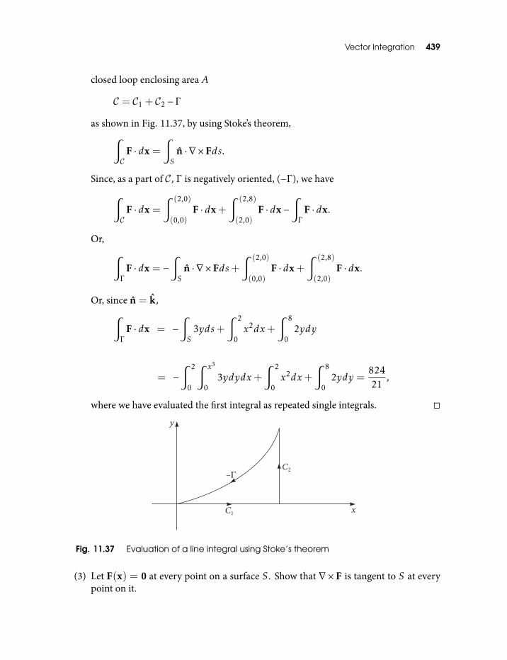
Vector Integration 439
closed loop enclosing area A
C = C1 + C2 − Γ
as shown in Fig. 11.37, by using Stoke’s theorem,∫C
F · dx =
∫S
n · ∇ ×Fds.
Since, as a part of C, Γ is negatively oriented, (−Γ ), we have∫C
F · dx =
∫ (2,0)
(0,0)F · dx+
∫ (2,8)
(2,0)F · dx−
∫Γ
F · dx.
Or, ∫Γ
F · dx = −∫S
n · ∇ ×Fds+∫ (2,0)
(0,0)F · dx+
∫ (2,8)
(2,0)F · dx.
Or, since n = k,∫Γ
F · dx = −∫S
3yds+∫ 2
0x2dx+
∫ 8
02ydy
= −∫ 2
0
∫ x3
03ydydx+
∫ 2
0x2dx+
∫ 8
02ydy =
82421
,
where we have evaluated the first integral as repeated single integrals.
Fig. 11.37 Evaluation of a line integral using Stoke’s theorem
(3) Let F(x) = 0 at every point on a surface S . Show that ∇× F is tangent to S at everypoint on it.
440 An Introduction to Vectors, Vector Operators and Vector Analysis
Solution Suppose ∇× F is not tangent to S at a point P on S . Then, by continuity,there is some neighborhood of P on S, say S ′, in which the component of∇×F alongthe normal n has the same sign, at every point in S ′ . Applying Stoke’s theorem to S ′,∫
Γ
F · dx =
∫S ′
n · ∇ ×Fds,
where Γ is the boundary of S ′ . Since F = 0 on S ′,∫Γ
F · dx = 0 on S ′ . However,∫S ′
n · ∇ × Fds , 0 on S ′, since the integrand is not zero by assumption and has thesame sign throughout S ′ . This contradicts Stoke’s theorem, so that n · ∇ × F = 0or ∇ × F must be perpendicular to n, that is, tangent to S at P . Since point P wasarbitrary, ∇×F is tangent to S at all points on it.
(4) Show that∫Γ
f (x)dx =
∫S
n×∇f ds, (11.184)
where Γ is the boundary of S .
Solution Let a be an arbitrary constant vector. Then, f (x)a is a vector. By Stoke’stheorem,∫
Γ
f (x)a · dx =
∫S
n · ∇ × f (x)ads
=
∫S
n · (f ∇× a+∇f × a)ds
=
∫S
n · (∇f × a)ds =∫S
a · (n×∇f )ds
as ∇× a = 0. This gives
a ·[∫
Γ
f (x)dx−∫S(n×∇f )ds
]= 0.
Since a is arbitrary, the second factor in the dot product must vanish, provingEq. (11.184).
(5) Show that∫Γ
dx×F =
∫S(n×∇)×Fds (11.185)
where Γ is the boundary of the surface S .
Vector Integration 441
Solution Let a be an arbitrary constant vector and consider∫Γ
a×F · dx = a ·∫Γ
F× dx.
By Stoke’s theorem,∫Γ
a×F · dx =
∫S
n · ∇ × (a×F)ds
=
∫S
n · [a(∇ ·F)− (a · ∇)F]ds
= a ·∫S[(∇ ·F)n−∇(F · n)]ds
= −a ·∫S(n×∇)×Fds.
All these steps can be proved using Levi-Civita symbols and noting that ∇ does notoperate on n. Last two equations give
a ·[∫
Γ
dx×F−∫S(n×∇)×Fds
]= 0.
Since a is arbitrary, the second factor of the dot product must vanish, provingEq. (11.185).
(6) Show that∣∣∣∫Γdx× x
∣∣∣ , where Γ is a closed curve in the xy plane, is twice the enclosedarea A.
Solution In Eq. (11.185) we replace n by k which is the vector normal to xy planeand F by x. We get,∫
Γ
dx× x =
∫S(k×∇)× xds
=
∫S[∇(k · x)− k(∇ · x)]ds
=
∫S(k− 3k)ds = −2k
∫Sds = −2kA,
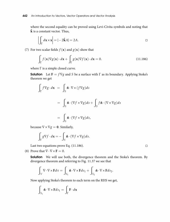
442 An Introduction to Vectors, Vector Operators and Vector Analysis
where the second equality can be proved using Levi-Civita symbols and noting thatk is a constant vector. Thus,∣∣∣∣∣∫
Γ
dx× x∣∣∣∣∣= | − 2kA|= 2A.
(7) For two scalar fields f (x) and g(x) show that∫Γ
f (x)∇g(x) · dx+∫Γ
g(x)∇f (x) · dx = 0. (11.186)
where Γ is a simple closed curve.
Solution Let F = f ∇g and S be a surface with Γ as its boundary. Applying Stoke’stheorem we get∫
Γ
f ∇g · dx =
∫S
n · ∇ × (f ∇g)ds
=
∫S
n · (∇f ×∇g)ds+∫Sf n · (∇×∇g)ds
=
∫S
n · (∇f ×∇g)ds,
because ∇×∇g = 0. Similarly,∫Γ
g∇f · dx = −∫S
n · (∇f ×∇g)ds.
Last two equations prove Eq. (11.186).
(8) Prove that ∇ ·∇×F = 0.
Solution We will use both, the divergence theorem and the Stoke’s theorem. Bydivergence theorem and referring to Fig. 11.37 we see that∫
V∇ ·∇×Fdτ =
∫S1
n · ∇ ×Fds1 +∫S2
n · ∇ ×Fds2.
Now applying Stoke’s theorem to each term on the RHS we get,∫S1
n · ∇ ×Fds1 =∫Γ
F · dx
Vector Integration 443
and ∫S2
n · ∇ ×Fds2 = −∫Γ
F · dx.
The sign is reversed while transforming the second integral because the positivedirections around the boundaries of the two surfaces are opposite. Hence,∫
V∇ ·∇×Fdτ = 0.
Since this equation holds for all volume elements it follows that ∇ · ∇ × F = 0. (9) For a closed surface S, show that
(i)∫S
n · (∇×F)ds = 0
and
(ii)∫S
n×∇f ds = 0.
Hints (i) Divide S into two parts, S1 and S2, with the common boundary curve Γ
(see Fig. 11.37) and write∫S
n · (∇×F)ds =∫S1
n · (∇×F)ds1 +∫S2
n · (∇×F)ds2.
Now, apply Stoke’s theorem to both the terms on RHS keeping in mind that thepositive sense of traversing Γ as the boundary of S1 is opposite to that traversing Γ asthe boundary of S2. This makes the two terms on RHS cancel after applying Stoke’stheorem and the result follows.(ii) Following the hint for part (i) we can write∫
Sn×∇f ds =
∫S1
n×∇f ds1 +∫S2
n×∇f ds2.
Now use Eq. (11.184) for the two terms on RHS and then follow rest of the hint forpart (i).
(10) Show that (with Γ as the boundary of S)∫Γ
f F · dx =
∫S
n · (∇f ×F+ f ∇×F)ds.
(11) If F is continuous and F× dx = 0 for every closed curve, show that F is constant.
12
Odds and Ends
In this chapter we present an assorted collection of situations to demonstrate how theycan be analyzed using vectors. Here, we do not attempt a systematic development of anyparticular topic. The basic idea is to illustrate how a large variety of problems can be tackledusing vectors in a coordinate free way.
12.1 Rotational Velocity of a Rigid BodyWe find the rotational velocity of an arbitrarily rotating rigid body. This section is acontinuation of our development of rotation operator and its matrix representation. Inparticular, we freely use the symbols introduced there, without re-defining them here.
Since the rotational velocity of a rigid body is common to all points of the body, it isenough to find the rotational velocity of the position vector x(t) of a point in the body. Letx0 denote the value of x(t) at t = 0. We seek a relation of the form
x = [ΩS]x0 =Ωx. (12.1)
and solve for Ω. Note that the time dependence must reside in the operator ΩS . Obviously,
Ω= SST = SS−1 (12.2)
solves Eq. (12.1) giving x = Sx0 where S is the time derivative of the operator S(t). Notethat we are using the same symbol for the operator and its matrix. This is justified becausethey are isomorphic. Differentiating SST = I we get
SST + SST = 0. (12.3)
Here, we have used the fact that the operations of transpose and differentiation commute.Equations (12.2) and (12.3) lead to
Ω= SST = −SST = −ΩT (12.4)
Odds and Ends 445
Thus, the operator Ω is skewsymmetric. We know that every skewsymmetric operator ona 3-D Euclidean space is the operator of vector multiplication by a fixed vector. We denotethe corresponding vector for the skewsymmetric operator Ω by ω, so that
Ωx = ω × x ∀x ∈R3.
To appreciate this result, consider the matrix of Ω in some basis0 −ω3 ω2
ω3 0 −ω1
−ω2 ω1 0
.
This gives vector ω ↔ [ω1 ω2 ω3]T as an eigenvector with eigenvalue 0. By applying the
matrix Ω to a vector x↔ [x1 x2 x3]T we get the vector ω × x↔ [ω2x3 −ω3x2 ω3x1 −
ω1x3 ω1x2 −ω2x1]T .
In order to get the expression for ω we proceed as follows. Put θn × x = Ax definingoperator A. Then, the equation connecting x0 at t = 0 with x(t) at a later time t, namely,
x = eθn×x0
can be written, in terms of A as
x = eAx0 (12.5)
whence S = eA. It then follows that
Ω=ddt
(eA
)e−A (12.6)
which can be expanded, giving
Ω= A+12![A, A] +
13![A, [A, A]] + · · · (12.7)
Here, [A,B] = AB−BA is the commutator of A and B. To prove Eq. (12.7) we define
Ω(λ) =∂∂t
(eλA
)e−λA
where λ is a parameter independent of t. We have Ω(0) = 0 and
∂Ω(λ)
∂λ= A+ [A,Ω(λ)].
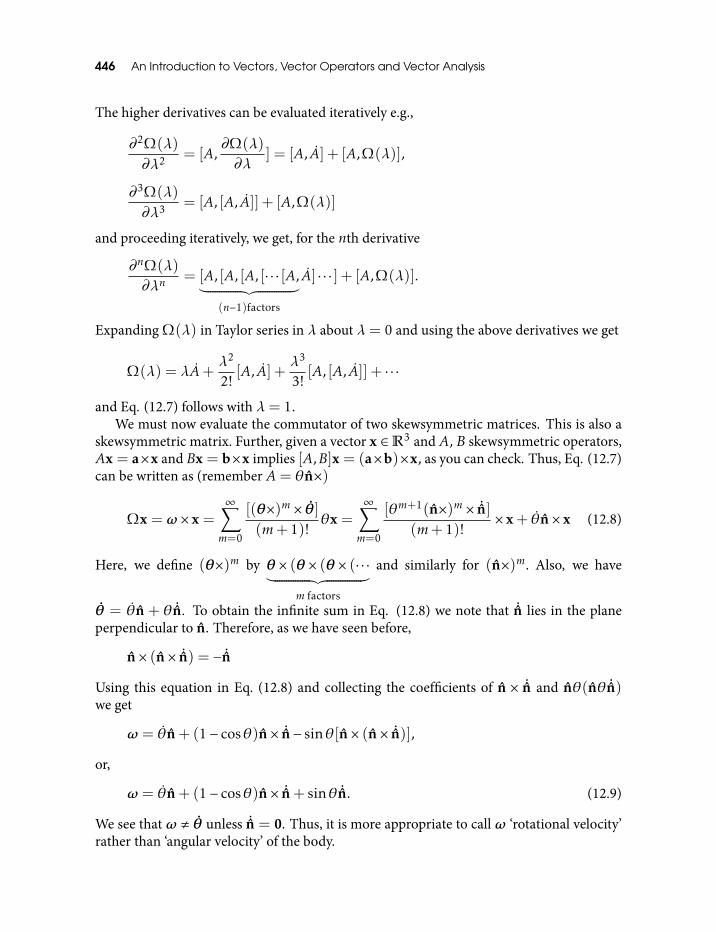
446 An Introduction to Vectors, Vector Operators and Vector Analysis
The higher derivatives can be evaluated iteratively e.g.,
∂2Ω(λ)
∂λ2 = [A,∂Ω(λ)
∂λ] = [A, A] + [A,Ω(λ)],
∂3Ω(λ)
∂λ3 = [A, [A, A]] + [A,Ω(λ)]
and proceeding iteratively, we get, for the nth derivative
∂nΩ(λ)
∂λn= [A, [A, [A, [· · · [A,︸ ︷︷ ︸
(n−1)factors
A] · · · ] + [A,Ω(λ)].
Expanding Ω(λ) in Taylor series in λ about λ= 0 and using the above derivatives we get
Ω(λ) = λA+λ2
2![A, A] +
λ3
3![A, [A, A]] + · · ·
and Eq. (12.7) follows with λ= 1.We must now evaluate the commutator of two skewsymmetric matrices. This is also a
skewsymmetric matrix. Further, given a vector x ∈R3 and A, B skewsymmetric operators,Ax = a×x and Bx = b×x implies [A,B]x = (a×b)×x, as you can check. Thus, Eq. (12.7)can be written as (remember A= θn×)
Ωx = ω × x =∞∑m=0
[(θ×)m × θ](m+ 1)!
θx =∞∑m=0
[θm+1(n×)m × ˙n](m+ 1)!
× x+ θn× x (12.8)
Here, we define (θ×)m by θ × (θ × (θ × (· · ·︸ ︷︷ ︸m factors
and similarly for (n×)m. Also, we have
θ = θn + θ ˙n. To obtain the infinite sum in Eq. (12.8) we note that ˙n lies in the planeperpendicular to n. Therefore, as we have seen before,
n× (n× ˙n) = − ˙n
Using this equation in Eq. (12.8) and collecting the coefficients of n × ˙n and nθ(nθ ˙n)we get
ω = θn+ (1− cosθ)n× ˙n− sinθ[n× (n× ˙n)],
or,
ω = θn+ (1− cosθ)n× ˙n+ sinθ ˙n. (12.9)
We see that ω , θ unless ˙n = 0. Thus, it is more appropriate to call ω ‘rotational velocity’rather than ‘angular velocity’ of the body.
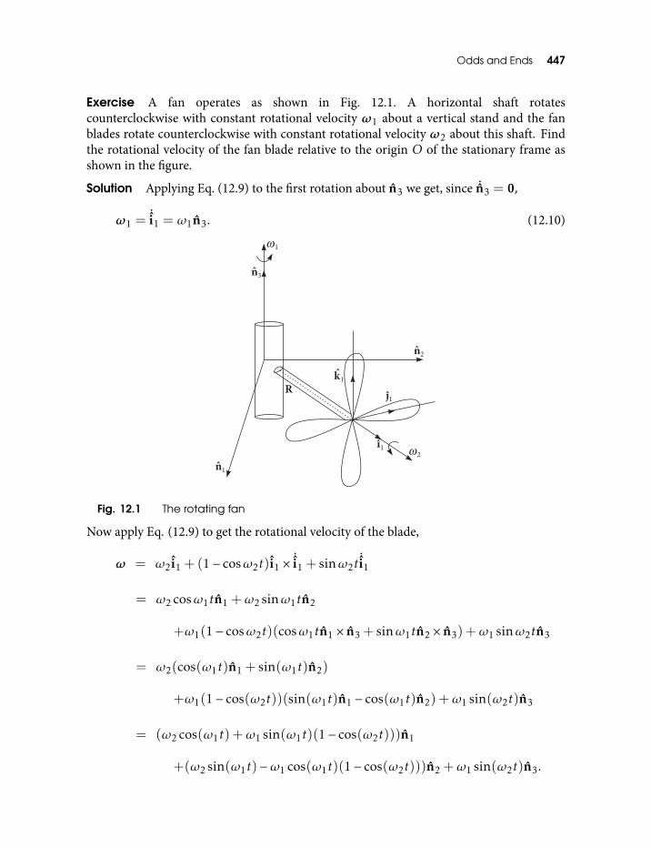
Odds and Ends 447
Exercise A fan operates as shown in Fig. 12.1. A horizontal shaft rotatescounterclockwise with constant rotational velocity ω1 about a vertical stand and the fanblades rotate counterclockwise with constant rotational velocity ω2 about this shaft. Findthe rotational velocity of the fan blade relative to the origin O of the stationary frame asshown in the figure.
Solution Applying Eq. (12.9) to the first rotation about n3 we get, since ˙n3 = 0,
ω1 =˙i1 = ω1n3. (12.10)
Fig. 12.1 The rotating fan
Now apply Eq. (12.9) to get the rotational velocity of the blade,
ω = ω2i1 + (1− cosω2t)i1 × ˙i1 + sinω2t˙i1
= ω2 cosω1tn1 +ω2 sinω1tn2
+ω1(1− cosω2t)(cosω1tn1 × n3 + sinω1tn2 × n3) +ω1 sinω2tn3
= ω2(cos(ω1t)n1 + sin(ω1t)n2)
+ω1(1− cos(ω2t))(sin(ω1t)n1 − cos(ω1t)n2) +ω1 sin(ω2t)n3
= (ω2 cos(ω1t) +ω1 sin(ω1t)(1− cos(ω2t)))n1
+(ω2 sin(ω1t)−ω1 cos(ω1t)(1− cos(ω2t)))n2 +ω1 sin(ω2t)n3.
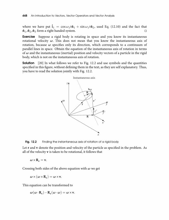
448 An Introduction to Vectors, Vector Operators and Vector Analysis
where we have put i1 = cosω1tn1 + sinω1tn2, used Eq. (12.10) and the fact thatn1, n2, n3 form a right handed system.
Exercise Suppose a rigid body is rotating in space and you know its instantaneousrotational velocity ω. This does not mean that you know the instantaneous axis ofrotation, because ω specifies only its direction, which corresponds to a continuum ofparallel lines in space. Obtain the equation of the instantaneous axis of rotation in termsof ω and the instantaneous (inertial) position and velocity vectors of a particle in the rigidbody, which is not on the instantaneous axis of rotation.
Solution [20] In what follows we refer to Fig. 12.2 and use symbols and the quantitiesspecified in this figure, without defining them in the text, as they are self explanatory. Thus,you have to read the solution jointly with Fig. 12.2.
Fig. 12.2 Finding the instantaneous axis of rotation of a rigid body
Let r and v denote the position and velocity of the particle as specified in the problem. Asall of the velocity v is taken to be rotational, it follows that
ω ×Rc = v.
Crossing both sides of the above equation with ω we get
ω × (ω ×Rc) = ω × v.
This equation can be transformed to
ω(ω ·Rc)−Rc(ω ·ω) = ω × v.
Odds and Ends 449
Now ω ·Rc = 0 and ω ·ω = |ω|2, so that
Rc =−(ω × v)|ω|2
.
Now
r′ = Rc +λω|ω|
=λω|ω|−(ω × v)|ω|2
,
where λ is a scalar parameter with the dimensions of length. Hence, we have, with R =r− r′,
R = r− λω|ω|
+(ω × v)|ω|2
.
As λ varies, the locus of the tip of this vector generates the line of the instantaneous axis ofrotation for a point moving with velocity v and position vector r in the rigid body. Since theinstantaneous rotational velocity ω is common to the whole rigid body, the instantaneousaxis of rotation we have found is also common to all points in the body.
12.2 3-D Harmonic OscillatorOscillatory motion is performed by systems close to their stable equilibrium configurationsunder specified force fields. Here, we deal with a particle moving under the action of aforce field f(x). We are concerned with an equilibrium point for the field, that is, thepoint x0 such that f(x0) = 0. Thus, the particle does not experience any force at x0. Weassume that x0 is an isolated equilibrium point, that is, it has a neighborhood devoid of anyequilibrium point other than itself. Shifting the origin to x0, the condition for equilibriumcan be stated as
f(0) = 0.
An equilibrium point is said to be stable, if it has a neighborhood at every point of whichthe particle is accelerated towards the interior of the neighborhood. A famous theorem dueto Lagrange states that an equilibrium point is stable if and only if it is a point of localminimum for the potential corresponding to the field.
Thus, we are interested in the bounded motion of a system near a stable equilibriumpoint. To get this motion, we must first get an approximate form of the force field in aneighborhood of the equilibrium point. This can be achieved if the field f(x) has a Taylorexpansion in some neighborhood of the stable equilibrium point which we have taken tobe the origin. We can then write
f(x) = f(0) + r · ∇f(0) +12(r · ∇)2f(0) + · · · .
450 An Introduction to Vectors, Vector Operators and Vector Analysis
The first term on RHS vanishes because origin is an equilibrium point, while the secondterm is linear in r, that is,
(α1r1 +α2r2) · ∇f(0) = α1r1 · ∇f(0) +α2r2 · ∇f(0).
Third and further terms are of higher order of smallness and can be neglected. Stability ofthe equilibrium point is ensured if we impose r · r < 0, or, equivalently, we use thefollowing stability condition,
r · ∇f(0) ≤ 0,
with equality only when r = 0.If we keep only the second term in the Taylor expansion of the force and neglect all
further higher order terms, the corresponding equation of motion is the following secondorder linear differential equation:
mr = r · ∇f(0).
Since this is a second order equation, it has two linearly independent solutions (that is,they are not proportional to each other) say r1 = r1(t) and r2 = r2(t). Since it is linear,any linear combination of these two linearly independent solutions say rn = αnr1(t)+βnr2(t) is also a solution. This system, governed by a linear force obeying the stabilitycondition, is called a harmonic oscillator . This superposition principle makes the analysisof harmonic oscillator manageable. As we will see below, if the force satisfies oneadditional requirement of being isotropic, the harmonic oscillator equation can beintegrated to get exact solutions. On the other hand, if we add the third term in the Taylorseries to the equation of motion, the resulting differential equation ceases to be linear. Themathematical analysis of this so called anharmonic oscillator becomes very difficult and isgenerally analysed using perturbation techniques, where the anharmonic term is treatedas a small perturbation to the harmonic one.
Let us now specialize to the case where the force f is not only linear, but also isotropicor central, that is, it is only a function of the magnitude of r and not of its direction. Thus,f(r) ≡ (f (r),0,0), expressed in the r, θ, φ basis. It is straightforward to check that in thiscase
r · ∇f(0) = −kr r = −kr, where −k =df(r)
dr
∣∣∣∣r=0
.
k is called the force constant and gives the strength of the isotropic binding force. Note that,if V (r) is the potential function for the isotropic force, df (r)dr
∣∣∣∣r=0
= −d2V (r)dr2
∣∣∣∣r=0
= −k. By
Lagrange’s theorem potential V (r) has a local minimum at r = 0 so that d2V (r)dr2
∣∣∣∣r=0
> 0,
making k > 0. This makes −k < 0 and satisfies the stability condition. The force −kr, (k >0), is commonly called Hooke’s law force after Robert Hooke, who invented it to explainthe elastic force causing oscillations of a spring. However, one has to remember that the
Odds and Ends 451
general form of the Hooke’s law force is given by the second term in the Taylor expansion ofany force field near a stable equilibrium position, thus giving an universal approximationto any force field having Taylor expansion near a stable equilibrium point. This explainswhy Hooke’s law is so ubiquitous in physics and engineering applications. By the sameargument, Hooke’s law is not a fundamental force law, but only a very useful approximation.
Thus, we have to solve the equation
r+ω20r = 0 where ω2
0 =km
. (12.11)
It turns out that bounded orbits of the attractive central force −kr are closed [3, 10, 19], sothat the motion in the vicinity of a stable equilibrium point under such a force is periodic.Further, note that the torque exerted by −kr on the particle is −kr× r = 0. Therefore, theangular momentum of the particle must be conserved. This fixes the angular momentumvectormr×v in space confining the position vector r and the velocity vector v of the particleto a plane perpendicular to the angular momentum vector. Thus, the motion under such acentral force is planar.
In order to get two linearly independent solutions of Eq. (12.11) let us choose one ofthem as the circular orbit obtained by rotating a vector a+ counterclockwise in the planeof the orbit through the angle ω0t in time t about the unit vector n perpendicular to theplane of the orbit. Using Eq. (6.45) we get,
r+(t) =Rn,ω0t(a+) = cosω0ta+ + sinω0t(n× a+). (12.12)
To construct the other linearly independent solution we take a vector a− in the plane of theorbit and rotate it clockwise by the angleω0t in time t. This amounts to replacing n by −nand a+ by a− in Eq. (12.12). We get,
r−(t) = cosω0ta− − sinω0t(n× a−). (12.13)
To get a general solution we add these two linearly independent solutions. We get,
r(t) = a0 cosω0t+b0 sinω0t, (12.14)
where
a0 = a+ + a−
and
b0 = (a+ − a−)× n. (12.15)
The two constant vectors a0 and b0 can have any values. Therefore, Eq. (12.14) is thegeneral solution of Eq. (12.11). If either a0 = 0 or b0 = 0, the motion becomes onedimensional with oscillations along the line of the surviving vector. Thus, the motionceases to be planar and the unit vector n is not uniquely defined, but any unit vectornormal to a± will do.
452 An Introduction to Vectors, Vector Operators and Vector Analysis
The vector coefficients a0 and b0 can be expressed in terms of initial conditions, thatis, the values of the position and velocity vectors at t = 0. Putting t = 0 in the expressionsfor r(t) as in Eq. (12.14) and r(t) obtained by differentiating Eq. (12.14) with respect to t,we get
r0 = r(0) = a0
v0 = r(0) = ω0b0. (12.16)
An inspection of Eq. (12.14) tells us that it represents a superposition of independent simpleharmonic motions along the lines determined by a0 and b0 or, via Eq. (12.16) along r0and v0. The resultant motion is elliptical and reduces to one-dimensional simple harmonicmotion if r0 = 0 or v0 = 0 or, generally, when r0×v0 = 0. To see that the orbit is an ellipsewe recast Eq. (12.14) as
r = acosφ+bsinφ, (12.17)
where a2 ≥ b2, a ·b = 0 and φ = φ(t) = ω0t+φ0. Vectors a and b define the major axisand the minor axis of the ellipse respectively.
Exercise For an oscillator with orbit
r(t) = acos(ω0t+φ0) +bsin(ω0t+φ0),
find the major axis a and the minor axis b from the initial conditions r0 = r(0) and v0 =r(0). Show that, for 0 < φ0 <
π2 ,
a = r0 cosφ0 −v0
ω0sinφ0
b = r0 sinφ0 +v0
ω0cosφ0
and that φ0 is given by
tan2φ0 =2ω0r0 · v0
v20 −ω
20r2
0
.
Hint Expand the trigonometric functions in the expression for r(t) and compare withEq. (12.14) to get expressions for a0 and b0 in terms of a and b and invert these equationsto get the result. To get the equation for φ0 use a ·b = 0.
We may eliminate φ0 by taking φ0 = ω0t0 and then shifting the origin in time to t0. Youmay recognize Eq. (12.17) to be the equation to an ellipse parameterized by φ which wehave encountered before (see section 2.4). a and b respectively give the major axis and the
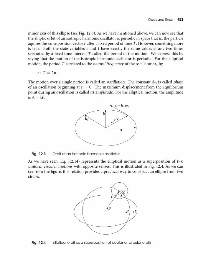
Odds and Ends 453
minor axis of this ellipse (see Fig. 12.3). As we have mentioned above, we can now see thatthe elliptic orbit of an isotropic harmonic oscillator is periodic in space that is, the particleaquires the same position vector r after a fixed period of time T . However, something moreis true. Both the state variables r and r have exactly the same values at any two timesseparated by a fixed time interval T called the period of the motion. We express this bysaying that the motion of the isotropic harmonic oscillator is periodic. For the ellipticalmotion, the period T is related to the natural frequency of the oscillator ω0 by
ω0T = 2π.
The motion over a single period is called an oscillation. The constant φ0 is called phaseof an oscillation beginning at t = 0. The maximum displacement from the equilibriumpoint during an oscillation is called its amplitude. For the elliptical motion, the amplitudeis A= |a|.
Fig. 12.3 Orbit of an isotropic harmonic oscillator
As we have seen, Eq. (12.14) represents the elliptical motion as a superposition of twouniform circular motions with opposite senses. This is illustrated in Fig. 12.4. As we cansee from the figure, this relation provides a practical way to construct an ellipse from twocircles.
Fig. 12.4 Elliptical orbit as a superposition of coplanar circular orbits
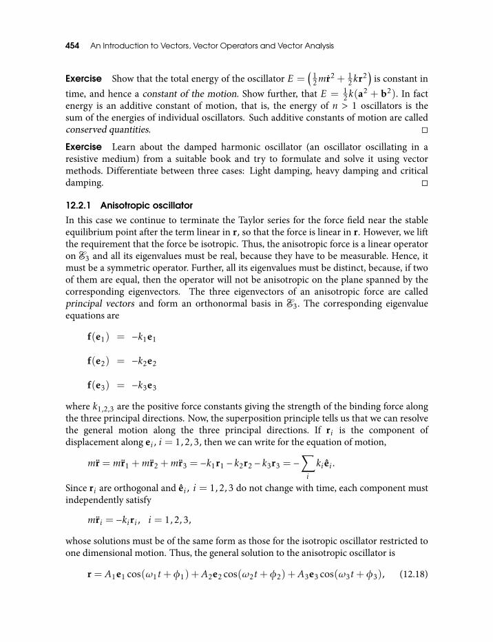
454 An Introduction to Vectors, Vector Operators and Vector Analysis
Exercise Show that the total energy of the oscillator E =(
12mr2 + 1
2kr2)
is constant intime, and hence a constant of the motion. Show further, that E = 1
2k(a2 + b2). In fact
energy is an additive constant of motion, that is, the energy of n > 1 oscillators is thesum of the energies of individual oscillators. Such additive constants of motion are calledconserved quantities.
Exercise Learn about the damped harmonic oscillator (an oscillator oscillating in aresistive medium) from a suitable book and try to formulate and solve it using vectormethods. Differentiate between three cases: Light damping, heavy damping and criticaldamping.
12.2.1 Anisotropic oscillator
In this case we continue to terminate the Taylor series for the force field near the stableequilibrium point after the term linear in r, so that the force is linear in r. However, we liftthe requirement that the force be isotropic. Thus, the anisotropic force is a linear operatoron E3 and all its eigenvalues must be real, because they have to be measurable. Hence, itmust be a symmetric operator. Further, all its eigenvalues must be distinct, because, if twoof them are equal, then the operator will not be anisotropic on the plane spanned by thecorresponding eigenvectors. The three eigenvectors of an anisotropic force are calledprincipal vectors and form an orthonormal basis in E3. The corresponding eigenvalueequations are
f(e1) = −k1e1
f(e2) = −k2e2
f(e3) = −k3e3
where k1,2,3 are the positive force constants giving the strength of the binding force alongthe three principal directions. Now, the superposition principle tells us that we can resolvethe general motion along the three principal directions. If ri is the component ofdisplacement along ei , i = 1,2,3, then we can write for the equation of motion,
mr =mr1 +mr2 +mr3 = −k1r1 − k2r2 − k3r3 = −∑i
ki ei .
Since ri are orthogonal and ei , i = 1,2,3 do not change with time, each component mustindependently satisfy
mri = −kiri , i = 1,2,3,
whose solutions must be of the same form as those for the isotropic oscillator restricted toone dimensional motion. Thus, the general solution to the anisotropic oscillator is
r = A1e1 cos(ω1t+φ1) +A2e2 cos(ω2t+φ2) +A3e3 cos(ω3t+φ3), (12.18)
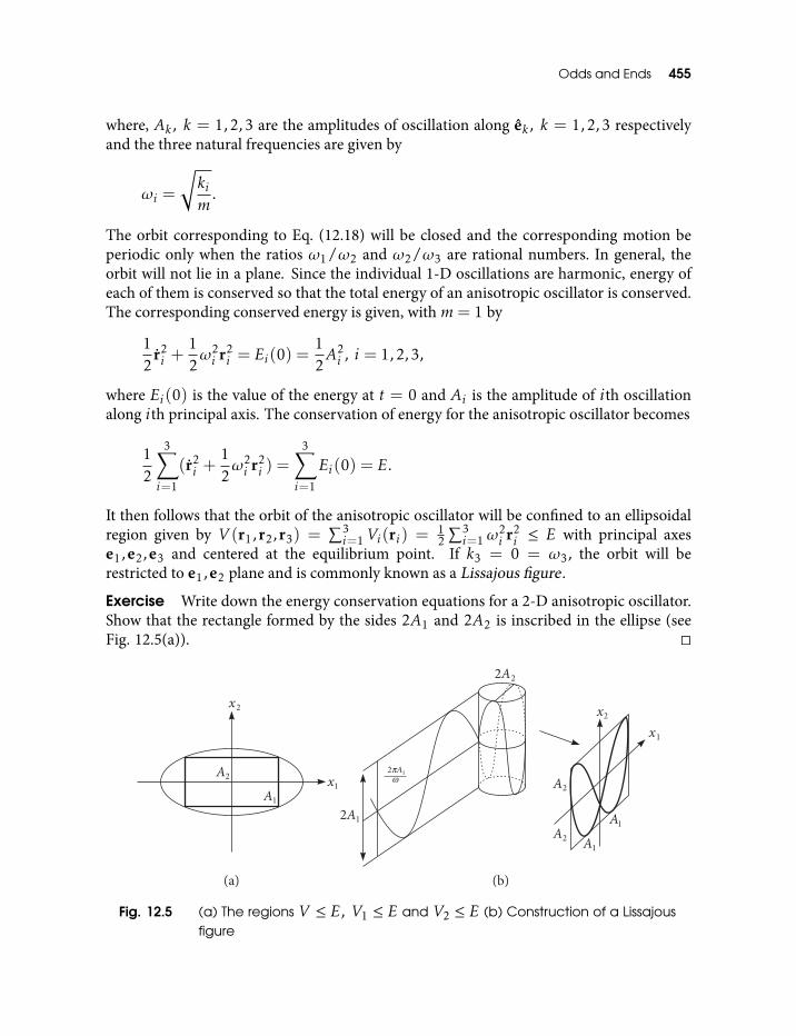
Odds and Ends 455
where, Ak , k = 1,2,3 are the amplitudes of oscillation along ek , k = 1,2,3 respectivelyand the three natural frequencies are given by
ωi =
√kim
.
The orbit corresponding to Eq. (12.18) will be closed and the corresponding motion beperiodic only when the ratios ω1/ω2 and ω2/ω3 are rational numbers. In general, theorbit will not lie in a plane. Since the individual 1-D oscillations are harmonic, energy ofeach of them is conserved so that the total energy of an anisotropic oscillator is conserved.The corresponding conserved energy is given, withm= 1 by
12
r2i +
12ω2i r2i = Ei(0) =
12A2i , i = 1,2,3,
where Ei(0) is the value of the energy at t = 0 and Ai is the amplitude of ith oscillationalong ith principal axis. The conservation of energy for the anisotropic oscillator becomes
12
3∑i=1
(r2i +
12ω2i r2i ) =
3∑i=1
Ei(0) = E.
It then follows that the orbit of the anisotropic oscillator will be confined to an ellipsoidalregion given by V (r1,r2,r3) =
∑3i=1Vi(ri) = 1
2∑3i=1ω
2i r2i ≤ E with principal axes
e1,e2,e3 and centered at the equilibrium point. If k3 = 0 = ω3, the orbit will berestricted to e1,e2 plane and is commonly known as a Lissajous figure .
Exercise Write down the energy conservation equations for a 2-D anisotropic oscillator.Show that the rectangle formed by the sides 2A1 and 2A2 is inscribed in the ellipse (seeFig. 12.5(a)).
Fig. 12.5 (a) The regions V ≤ E, V1 ≤ E and V2 ≤ E (b) Construction of a Lissajousfigure
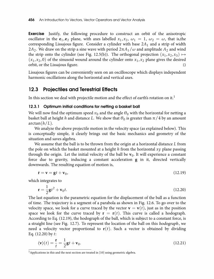
456 An Introduction to Vectors, Vector Operators and Vector Analysis
Exercise Justify, the following procedure to construct an orbit of the anisotropicoscillator in the e1,e2 plane, with axes labelled x1,x2, ω1 = 1, ω2 = ω, that is,thecorresponding Lissajous figure. Consider a cylinder with base 2A1 and a strip of width2A2. We draw on the strip a sine wave with period 2πA1/ω and amplitude A2 and windthe strip onto the cylinder (see Fig. 12.5(b)). The orthogonal projection (x1,x2,x3) 7→(x1,x2,0) of the sinusoid wound around the cylinder onto x1,x2 plane gives the desiredorbit, or the Lissajous figure.
Lissajous figures can be conveniently seen on an oscilloscope which displays independentharmonic oscillations along the horizontal and vertical axes.
12.3 Projectiles and Terestrial Effects
In this section we deal with projectile motion and the effect of earth’s rotation on it.1
12.3.1 Optimum initial conditions for netting a basket ball
We will now find the optimum speed v0 and the angle θ0 with the horizontal for netting abasket ball at height h and distance L. We show that θ0 is greater than π/4 by an amountarctan(h/L).
We analyze the above projectile motion in the velocity space (as explained below). Thisis conceptually simple, it clearly brings out the basic mechanics and geometry of thesituation and saves algebra.
We assume that the ball is to be thrown from the origin at a horizontal distance L fromthe pole on which the basket mounted at a height h from the horizontal xy plane passingthrough the origin. Let the initial velocity of the ball be v0. It will experience a constantforce due to gravity, inducing a constant acceleration g in it, directed verticallydownwards. The resulting equation of motion is,
r = v = gt+ v0, (12.19)
which integrates to
r =12
gt2 + v0t. (12.20)
The last equation is the parametric equation for the displacement of the ball as a functionof time. The trajectory is a segment of a parabola as shown in Fig. 12.6. To go over to thevelocity space, we look for a curve traced by the vector v = v(t), just as in the positionspace we look for the curve traced by r = r(t). This curve is called a hodograph.According to Eq. (12.19), the hodograph of the ball, which is subject to a constant force, isa straight line (see Fig. 12.7). To represent the location of the ball on this hodograph , weneed a velocity vector proportional to r(t). Such a vector is obtained by dividingEq. (12.20) by t:
〈v〉(t) = rt=
12
gt+ v0. (12.21)
1Applications in this and the next section are treated in [10] using geometric algebra.
Odds and Ends 457
Fig. 12.6 Trajectory in position space
The vector 〈v〉(t) is the average velocity of the ball. Note that 〈v〉(t) and r(t) have thesame direction. Comparing Eqs (12.19) and (12.21), we get a simple relation between theactual velocity and the average velocity:
v(t) = 〈v〉(t) + 12
gt =rt+
12
gt. (12.22)
Figure 12.6 depicts the hodograph given by Eq. (12.21) and also displays Eq. (12.22). Wesee that the increment in the velocity of the ball in equal intervals of time is equal.Fig. 12.7 contains all the information about the projectile motion, so all questionsregarding the motion can be answered by dealing with the triangles in the figuregraphically or algebraically.
Fig. 12.7 Trajectory in the velocity space
First, consider the question of determining the range r of a target sighted in a direction r(not necessarily along the horizontal) which is hit by a projectile, launched with velocityv0. This can be done graphically by using the properties of Fig. 12.7. Having laid out v0on a graph paper (by choosing appropriate units and scale!) as indicated in Fig. 12.7, oneextends a line from the base of v0, in the direction r, to its intersection with the vertical lineextending from the tip of v0. The length of the two sides of the triangle thus constructedare then measured, say v1 and v2, to get the magnitude of 1
2 gt and rt respectively. This gives
the time of flight t = 2v1/g and the range r = 2(v1v2)/g . How to get the final velocity isalso evident from Fig. 12.7.
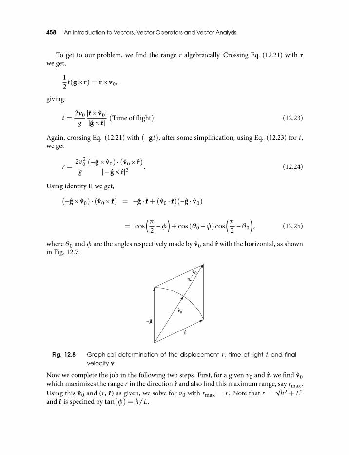
458 An Introduction to Vectors, Vector Operators and Vector Analysis
To get to our problem, we find the range r algebraically. Crossing Eq. (12.21) with rwe get,
12t(g× r) = r× v0,
giving
t =2v0
g|r× v0||g× r|
(Time of flight). (12.23)
Again, crossing Eq. (12.21) with (−gt), after some simplification, using Eq. (12.23) for t,we get
r =2v2
0g
(−g× v0) · (v0 × r)| − g× r|2
. (12.24)
Using identity II we get,
(−g× v0) · (v0 × r) = −g · r+ (v0 · r)(−g · v0)
= cos(π
2−φ
)+ cos (θ0 −φ)cos
(π2−θ0
), (12.25)
where θ0 and φ are the angles respectively made by v0 and r with the horizontal, as shownin Fig. 12.7.
Fig. 12.8 Graphical determination of the displacement r , time of light t and finalvelocity v
Now we complete the job in the following two steps. First, for a given v0 and r, we find v0which maximizes the range r in the direction r and also find this maximum range, say rmax.Using this v0 and (r , r) as given, we solve for v0 with rmax = r . Note that r =
√h2 + L2
and r is specified by tan(φ) = h/L.
Odds and Ends 459
To find the direction v0 which maximizes the range r along r, we note that r ismaximum when the RHS of Eq. (12.25) is maximum. Since r and −g are fixed directions,we have to maximize the second term on the RHS of Eq. (12.25). This is maximum whenπ2 −θ0 = θ0 −φ which implies θ0 = π
4 +φ2 . Thus, v0 is directed along the line bisecting
the angle between r and −g (see Fig. 12.8).Thus,
v0 =r− g|r− g|
. (12.26)
Substituting Eq. (12.26) in Eq. (12.24) we get,
rmax =2v2
0g
1|r− g|2
=v2
0g
11+ sin(φ)
. (12.27)
We leave the last equality for you to check. Solving Eq. (12.27) for v0 with rmax =√h2 + L2 = r0 say, (note that sin(φ) = h/r0), we get
v0 =√g(r0 + h).
Using θ0 =π4 +
φ2 and φ = arctan(h/L) we get
θ0 =π4+
12
arctan(hL
).
12.3.2 Optimum angle of striking a golf ball
For non-spinning high speed golf balls the force of air drag is roughly linear with velocity(FD = Cv). Assume that C/m = 0.25 s−1, m = 0.046 kg and that the maximumhorizontal range of 152 m is obtained with an initial speed of 61 m/sec. We show that theangle of striking has to be 32 degrees with the horizontal, whereas in the absence of anyair drag it would have been 45 degrees.
We have to set up and solve the equation of motion for a ball projected with the initialvelocity v0 from origin under the force of linear drag and constant gravity. Let the dragforce be given by
FD = Cv = −mγv.
which defines γ . Then the equation of motion is
v = g−γv, (12.28)
or,
(v+ γv) = g.
460 An Introduction to Vectors, Vector Operators and Vector Analysis
Noting that eγt is the integrating factor, we get,
eγt(v+ γv) =ddt
(eγtv) = eγtg.
Integrating, we get,
eγtv(t)− v0 = g∫ t
0eγt
′dt′ = g
(eγt − 1γ
).
Solving for v(t), we get,
v(t) = g(
1− e−γt
γ
)+ v0e
−γt. (12.29)
The constant γ−1 is called relaxation time which is the measure of the time it takes for theretarding force to make the particle forget its initial conditions. If t γ−1, then e−γt << 1so that the first term on the RHS of Eq. (12.29) dominates all others, irrespective of thevalue of v0, giving
v = v∞ = γ−1g.
The value v∞ is called the terminal velocity, which can also be obtained by putting v = 0in the equation of motion.
The displacement r of the ball from the origin is found by directly integratingEq. (12.29). This gives
r = g(e−γt + γt − 1
γ2
)+ v0
(1− e−γt
γ
). (12.30)
Let the plane of motion of the ball be the x−y plane with x axis horizontal. Equation (12.30)gives rise to the equations
x = v0x
(1− e−γt
γ
)(12.31)
y = g
(e−γt + γt − 1
γ2
)+ v0y
(1− e−γt
γ
). (12.32)
At the end of its range, the ball touches the ground, so y = 0, making the RHS ofEq. (12.32) equal to zero. This gives a transcendental equation for the time of flight twhich does not have a closed form solution. Assuming t to be sufficiently large so as tomake e−γt small enough, we expand e−γt in powers of t and retain terms only up tosecond order so that contribution due to gravity is properly included. We now find thepositive root of the resulting quadratic in t and substitute in Eq. (12.31). Putting
Odds and Ends 461
v0x = v0 cosθ0 and v0y = v0 sinθ0 where θ0 is the angle at which the ball is projectedand v0 = |v0|, we find that we have now got an equation expressing the range x as afunction of θ0. To find θ0 for the maximum range, we solve dx
dθ0= 0. Using the given
data, we get θmax0 = 320.
Equation (12.28) is useful in the analysis of microscopic motions also. For example,consider an electron (with mass m and charge e) moving in a conductor under theinfluence of a constant electric field E. The electron’s motion is retarded by the collisionswith the lattice. We may represent the retardation by the resistive force proportional to thevelocity of the electron. If the resistance is independent of the direction in which theelectron moves, we say that the conductor is an isotropic medium. We can then write theresistive force in the form −µv, where µ is a scalar constant. We are thus led to theequation, (compare with Eq. (12.28)),
v = eE−µv. (12.33)
For times large compared to the relaxation time τ = m/µ, the electron reaches theterminal velocity
v =
[eµ
]E (12.34)
and the result is a steady current in the conductor. The electric current density J is given by
J = Nev, (12.35)
where N is the number density of electrons. Substituting Eq. (12.34) in Eq. (12.35) we getOhm’s law
J = σE, (12.36)
where the conductor’s d-c conductivity σ is given by
σ = Ne2/µ. (12.37)
Ohm’s law holds remarkably well for many conductors over a wide range of currents. Theconductivity σ and the electron density N can be measured, so µ can be calculated fromEq. (12.37). Then, the relaxation time can also be calculated and compared with themeasured values. These are in general agreement with the extremely short relaxationtimes observed in metals. Thus, Eq. (12.33) is vindicated to some degree. However, wenote that the velocity v in Eq. (12.33) cannot be regarded as the velocity of an individualelectron, whose trajectory must be very irregular as it collides repeatedly with the massiveatoms in the lattice. Thus, v in Eq. (12.33) must be a kind of average electron velocity.Thus, our classical analysis can describe, (if at all), only the average motion in themicroscopic domain. Derivation and explanation of equations like Eq. (12.33), pertainingto the electron’s motion in a metal, requires statistical mechanics and the basic equationsof quantum mechanics.
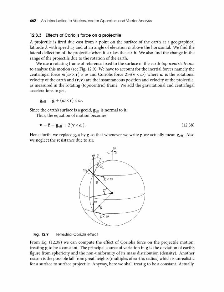
462 An Introduction to Vectors, Vector Operators and Vector Analysis
12.3.3 Effects of Coriolis force on a projectile
A projectile is fired due east from a point on the surface of the earth at a geographicallatitude λ with speed v0 and at an angle of elevation α above the horizontal. We find thelateral deflection of the projectile when it strikes the earth. We also find the change in therange of the projectile due to the rotation of the earth.
We use a rotating frame of reference fixed to the surface of the earth topocentric frameto analyse this motion (see Fig. 12.9). We have to account for the inertial forces namely thecentrifugal force m(ω × r) × ω and Coriolis force 2m(v × ω) where ω is the rotationalvelocity of the earth and (r,v) are the instantaneous position and velocity of the projectile,as measured in the rotating (topocentric) frame. We add the gravitational and centrifugalaccelerations to get,
geff = g+ (ω × r)×ω.
Since the earth’s surface is a geoid, geff is normal to it.Thus, the equation of motion becomes
v = r = geff+ 2(v×ω). (12.38)
Henceforth, we replace geff by g so that whenever we write g we actually mean geff. Alsowe neglect the resistance due to air.
Fig. 12.9 Terrestrial Coriolis effect
From Eq. (12.38) we can compute the effect of Coriolis force on the projectile motion,treating g to be a constant. The principal source of variation in g is the deviation of earth’sfigure from sphericity and the non-uniformity of its mass distribution (density). Anotherreason is the possible fall from great heights (multiples of earth’s radius) which is unrealisticfor a surface to surface projectile. Anyway, here we shall treat g to be a constant. Actually,
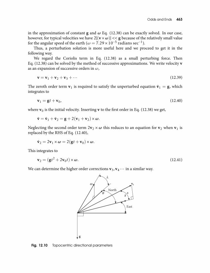
Odds and Ends 463
in the approximation of constant g and ω Eq. (12.38) can be exactly solved. In our case,however, for typical velocities we have 2|(v×ω)| << g because of the relatively small valuefor the angular speed of the earth (ω = 7.29× 10⁻⁵ radians sec−1).
Thus, a perturbation solution is more useful here and we proceed to get it in thefollowing way.
We regard the Coriolis term in Eq. (12.38) as a small perturbing force. ThenEq. (12.38) can be solved by the method of successive approximations. We write velocity vas an expansion of successive orders in ω,
v = v1 + v2 + v3 + · · · (12.39)
The zeroth order term v1 is required to satisfy the unperturbed equation v1 = g, whichintegrates to
v1 = gt+ v0, (12.40)
where v0 is the initial velocity. Inserting v to the first order in Eq. (12.38) we get,
v = v1 + v2 = g+ 2(v1 + v2)×ω.
Neglecting the second order term 2v2 ×ω this reduces to an equation for v2 when v1 isreplaced by the RHS of Eq. (12.40),
v2 = 2v1 ×ω = 2(gt+ v0)×ω.
This integrates to
v2 = (gt2 + 2v0t)×ω. (12.41)
We can determine the higher order corrections v3,v4 · · · in a similar way.
Fig. 12.10 Topocentric directional parameters
464 An Introduction to Vectors, Vector Operators and Vector Analysis
Substituting Eqs (12.40) and (12.41) in Eq. (12.39) we get the velocity to the first order inω as
v = v0 + gt+ (gt2 + 2v0t)×ω (12.42)
Integrating this, we get a parametric equation for the displacement
r =12
gt2 + v0t+∆r (12.43)
where the deviation ∆r from a parabolic trajectory (due to Coriolis force) is given to thefirst order by
∆r = (v0 +13
gt)×ωt2 + · · · (12.44)
To estimate the magnitude of the correction ∆r, we observe from Eqs (12.43) and (12.44)that
|∆r||r|≈ωt (12.45)
For the correction to be one percent we must have ωt ≥ 0.01 and from the value of ω wefind that the time of flight must be at least two minutes, which is more than the time of flightin a typical projectile problem. Hence, we need not consider the corrections of order higherthan the first. Indeed, before considering the higher order corrections, the assumption thatg is a constant should be examined.
The expression in Eq. (12.44) for the Coriolis deflection ∆r is not in its most convenientform as it is not given as a function of target location r. To circumvent this, we use the zerothorder approximation
r ≈ 12
gt2 + v0t (12.46)
to eliminate v0 in Eq. (12.44), with the result,
∆r = −tω × (r− 16
gt2). (12.47)
This shows the directional dependence of ∆r on r. To eliminate t from Eq. (12.47) in favourof r we cross both sides of Eq. (12.47) with g to get,
(r× g) = (v0 × g)t,
or,
(r× g) · (v0 × g) = |v0 × g|2t,
Odds and Ends 465
or,
t =(r× g) · (v0 × g)|v0 × g|2
. (12.48)
Similarly, again from Eq. (12.46) we have,
12t2 =
(r× v0) · (g× v0)
|g× v0|2. (12.49)
Note that
r− 16
gt2 = r
(r− 1
3
[(r× v0) · (g× v0)
|g× v0|2
]g)
. (12.50)
This shows that the two terms in Eq. (12.47) are of the same order of magnitude.To find the change in range due to the Coriolis force we have to find the component of
∆r in the direction r, which is easily obtained from Eq. (12.47) as
r ·∆r =t3
6r · (ω × g). (12.51)
Similarly, the vertical deflection is given by
g ·∆r = tr · (ω × g) (12.52)
The vector ω × g is directed west, except at poles, so both Eqs (12.51) and (12.52) vanishfor the trajectories to the north or south. They have maximum values for the trajectories tothe west. This is due to rotation of the earth in opposite direction while the projectile is inflight.
In most circumstances, resistive forces have a greater effect on the range and verticaldeflection than the Coriolis force. The lateral Coriolis deflection is more significant as itwill not be masked by resistive forces, that is, the observed lateral deflection is solely due toCoriolis force, as the resistive forces do not have any component in the lateral direction. Ofcourse, resistive forces will change ∆r (and also its lateral component) via their influenceon the velocity which in turn governs the Coriolis force.
For a target on a horizontal plane, g · r = 0 and g × r is a rightward unit vector. FromEq. (12.47), then, the rightward deflection ∆R is given by
∆R = (g× r) ·∆r
= −t(g× r) ·(ω ×
(r− t
2
6g))
= −t[(g ·ω)
(r ·
(r− t
2
6g))−(g ·
(r− t
2
6g))(r ·ω)
]
466 An Introduction to Vectors, Vector Operators and Vector Analysis
= t
[−r(g ·ω)− t
2
6g(r ·ω)
]
= −rtω ·(g+
t2g
6rr)
= −rtω ·(g+
13(r× v0) · (g× v0)
(g× v0) · (g× v0)r)
.
Here, we have used Eq. (12.49). We now use the identity II and Fig. 12.10 to get
∆R= rtωcosλ(tanλ− 13
tanα cosφ). (12.53)
For nearly horizontal trajectories (α ≈ 0), the second term in Eq. (12.53) can be neglected,giving ∆R = rtω sinλ which is positive in the northern hemisphere and negative in thesouthern hemisphere. As a general rule, therefore, the Coriolis force tends to deflectparticles to the right in the northern hemisphere and to the left in the southernhemisphere. However, this rule is violated by highly arched trajectories and Eq. (12.53)tells us that for a trajectory satisfying
tanα0 =3tanλcosφ
, (12.54)
the Coriolis deflection ∆R vanishes. In the northern hemisphere, deflection will be to theleft for α > α0 and to the right for α < α0. In the southern hemisphere, these inequalitiesreverse.
From Eq. (12.48), the time of flight for a target on the horizontal plane is
t =r
v0 cosα. (12.55)
Since the projectile is fired due east, φ = π2 , so from Eq. (12.53) we get,
∆R= rtω sinλ. (12.56)
We eliminate t from Eq. (12.56) using Eq. (12.55) to get,
∆R=
(r2
v0
)ω secα sinλ (12.57)
with obvious dependence on the hemisphere.To get the change in range for a projectile fired due east, we note that the angle between
r and ω× g is π. So (ω ×g) · r = −ωg cosλ. Substituting this result and the expression forthe time of flight from Eq. (12.55) into Eq. (12.51) we get,
Odds and Ends 467
Change in range = −16
(rv0
)3
ωg sec3α cosλ
which does not depend on the hemisphere.
Exercise River Brahamaputra flows southwards near Guwahati. Find the difference inwater levels at its right and left banks if its width is 5000 meters, the latitude of Guwahatiis 2611′ and its speed is 10 km/hr.
Solution It is observed that the Coriolis effect denudes the right banks of large rivers inthe northern hemisphere flowing over long stretches more than their left banks. On therivers in the southern hemisphere, the effect is opposite. The following solution to thisexercise will help you understand this.
We set up the topocentric coordinate system with its x-axis along the flow(southwards), y axis along the transverse horizontal direction to the left of the flow(eastward) and the local vertical along the z axis. Let the direction of the flow make anangle φ (in the anticlockwise sense) with respect to the geographical north direction.Since the river is flowing southwards, φ = π. (Now draw a figure). In this frame, therotational velocity of the earth and the velocity of the river v can be resolved as
ω = ω(sinλ k+ cosλcosφ i− cosλsinφ j)
and
v = vi.
Here, i, j, k are the unit vectors along x,y,z axes respectively. With φ = π the Coriolisacceleration ac becomes
ac = 2v×ω = −2vω sinλ j, (12.58)
which is towards the right of the flow (westward). So the total acceleration of the water isac + g (see Fig. 12.11) with ac given by Eq. (12.58). From Fig. 12.11 we see that the anglemade by the resultant ac+ g with g (angle α in Fig. 12.11) is given by
tanα =
(acg
). (12.59)
Now the water surface must be normal to the vector ac + g, so it makes angle α with thehorizontal. If the level difference is h and width of the river isW we have from Eq. (12.59),(
hW
)=
(acg
)
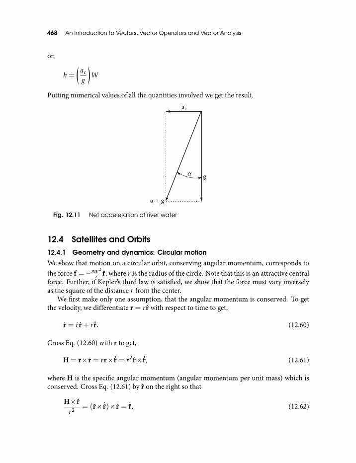
468 An Introduction to Vectors, Vector Operators and Vector Analysis
or,
h=
(acg
)W
Putting numerical values of all the quantities involved we get the result.
Fig. 12.11 Net acceleration of river water
12.4 Satellites and Orbits12.4.1 Geometry and dynamics: Circular motion
We show that motion on a circular orbit, conserving angular momentum, corresponds tothe force f = −mv2
r r, where r is the radius of the circle. Note that this is an attractive centralforce. Further, if Kepler’s third law is satisfied, we show that the force must vary inverselyas the square of the distance r from the center.
We first make only one assumption, that the angular momentum is conserved. To getthe velocity, we differentiate r = r r with respect to time to get,
r = r r+ r ˙r. (12.60)
Cross Eq. (12.60) with r to get,
H = r× r = rr× ˙r = r2r× ˙r, (12.61)
where H is the specific angular momentum (angular momentum per unit mass) which isconserved. Cross Eq. (12.61) by r on the right so that
H× rr2 = (r× ˙r)× r = ˙r, (12.62)
Odds and Ends 469
where we have used the identity I and the fact that r · ˙r = 0. We substitute Eq. (12.62) inEq. (12.60) to get
r = r r+H× rr
. (12.63)
To get the acceleration we differentiate Eq. (12.63) with respect to t and again useEq. (12.62) and identity I. We have,
r =(r − H
2
r3
)r. (12.64)
Now, we make use of the assumption that the motion is circular. This means H = rv,where v is the constant speed of the particle on the circle and also r = 0 = r . Therefore,the acceleration is
r = −v2
rr
and the force is
f =mr = −mv2
rr. (12.65)
Let us now assume that Kepler’s third law is valid i.e., r3
P 2 is a constant say C, where P isthe period of the orbit. For circular motion the period P is related to v by v = 2πr
P or,
v2 =4π2r2
P 2 .
Putting 1P 2 = C
r3 in this equation we get
v2 = 4π2Cr
. (12.66)
Put Eq. (12.66) in Eq. (12.65) to get
f = −4π2Cm
r2 r.
Thus, the conservation of angular momentum and Kepler’s third law mean that, for circularmotion, the force exerted on a moving particle is central, attractive and varies inversely asthe square of the radius of the circle.
470 An Introduction to Vectors, Vector Operators and Vector Analysis
Exercise The turning points of a satellite orbit are defined by the condition v · r = 0.Show that, for a turning point, the conservation of Runge–Lenz vector gives the relation
r =K
2E′(e− r), (12.67)
where E′ is the specific energy (energy per unit mass) and K is the constant in thegravitational force law.
The conservation of the Runge–Lenz (or the eccentricity) vector e is given by
v×H = K(e+ r), (12.68)
where H is the angular momentum per unit mass (specific angular momentum). PutH = r× v and use the identity I to get
v2r − (r · v) = K(e+ r). (12.69)
At the turning point r·v = 0, so the second term on the LHS vanishes. Further, v2 is relatedto E′ by [19]
v2 = 2(E′ +
Kr
). (12.70)
Substitute this expression for v2 in Eq. (12.69) to get
2(E′ +
Kr
)r = K(e+ r),
which easily simplifies to Eq. (12.67). It is instructive to sketch this relation on an ellipticor hyperbolic orbit. Note that Eq. (12.67) specifies the turning points only in terms of theconserved quantities.
12.4.2 Hodograph of an orbit
We find the hodograph for the Keplerian orbit of a satellite/spacecraft, that is, a curve overwhich the tip of the velocity vector moves as the satellite moves on its orbit.
We know that a Keplerian orbit is a consequence of the conservation of the eccentricityvector given by
v×H = K(e+ r), (12.71)
so it is no surprise that the hodograph, (which is the orbit in the velocity space), followsdirectly from it. Take the vector product with H on both sides of Eq. (12.71) to get
H× (v×H) = KH× (e+ r). (12.72)
Odds and Ends 471
Using identity I on the LHS of Eq. (12.72) we get,
H2v− (H · v)H = KH× (e+ r).
Since H · v = 0, we get,
v =KH
(H× e+ H× r). (12.73)
Since H× e is a constant vector, let us put
u =KH(H× e), (12.74)
so that
v−u =KH
(H× r) (12.75)
or, squaring both sides,
(v−u)2 =K2
H2 . (12.76)
This equation describes a circle of radius (K/H) centered at point u given by Eq. (12.74).Since the centre of the circle is determined by the eccentricity vector as in Eq. (12.74),
the distance u = |u| of the centre from the origin is used to classify the orbits as shown inthe following table. In the fourth column, we use |K | to make room for both attractive (K >0) and repulsive (K < 0) inverse square law force, (for example, Coulomb force betweentwo like charges, where K = −q1q2 < 0), although here we have assumed attractive inversesquare law (Newtonian gravity), as we are dealing with spacecrafts and satellites.
Table 12.1 Classification of Orbits with H , 0
Conic section Eccentricity Energy Hodograph centre
Hyperbola e > 1 E′ > 0 u > |K |H
parabola e = 1 E′ = 0 u = |K |H
Ellipse 0 < e < 1 E′ < 0 u < |K |H
Cirle e = 0 E′ = − K2
2H2 u = 0
Thus, the orbit is an ellipse if the origin is inside the circle, or an hyperbola if the origin isoutside the circle. For an elliptical orbit the hodograph described by Eq. (12.73) is a singlecomplete circle, as shown in Fig. 12.12 You may check the consistancy of Fig. 12.12 withEq. (12.73). Notice how, by parallelly moving any velocity vector v on the hodograph, wecan determine the corresponding position r on the orbit.
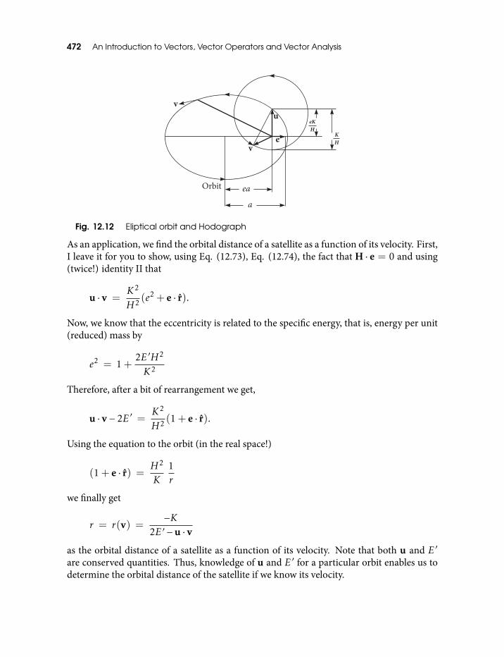
472 An Introduction to Vectors, Vector Operators and Vector Analysis
Fig. 12.12 Eliptical orbit and Hodograph
As an application, we find the orbital distance of a satellite as a function of its velocity. First,I leave it for you to show, using Eq. (12.73), Eq. (12.74), the fact that H · e = 0 and using(twice!) identity II that
u · v =K2
H2 (e2 + e · r).
Now, we know that the eccentricity is related to the specific energy, that is, energy per unit(reduced) mass by
e2 = 1+2E′H2
K2
Therefore, after a bit of rearrangement we get,
u · v− 2E′ =K2
H2 (1+ e · r).
Using the equation to the orbit (in the real space!)
(1+ e · r) =H2
K1r
we finally get
r = r(v) =−K
2E′ −u · v
as the orbital distance of a satellite as a function of its velocity. Note that both u and E′are conserved quantities. Thus, knowledge of u and E′ for a particular orbit enables us todetermine the orbital distance of the satellite if we know its velocity.
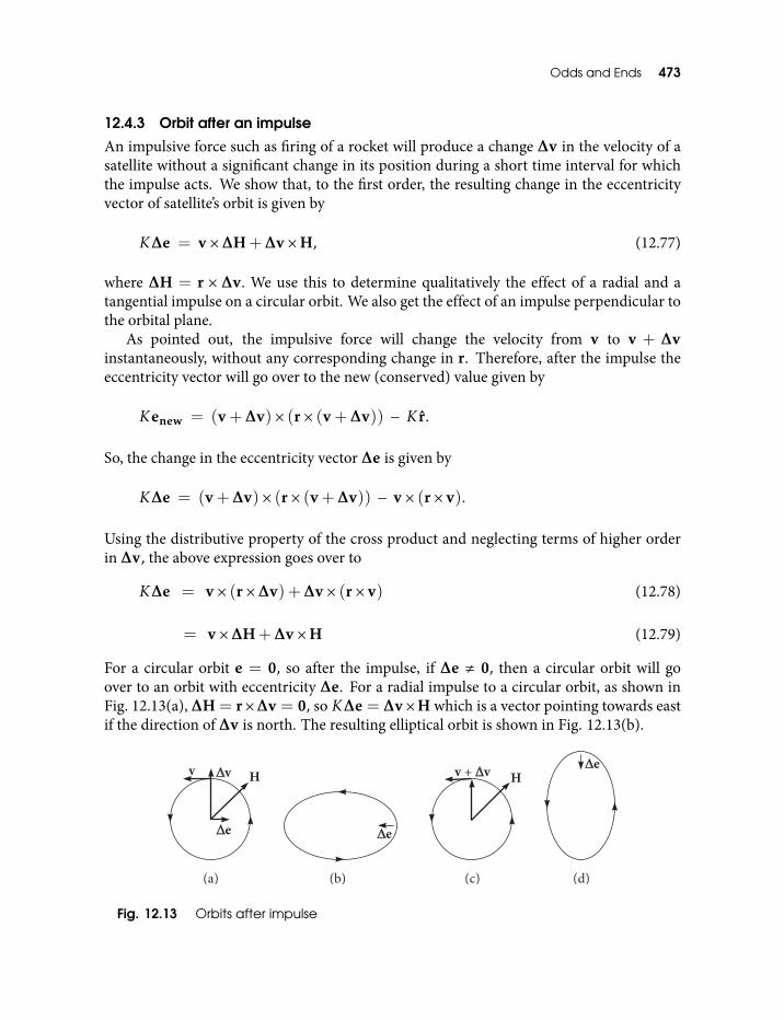
Odds and Ends 473
12.4.3 Orbit after an impulse
An impulsive force such as firing of a rocket will produce a change ∆v in the velocity of asatellite without a significant change in its position during a short time interval for whichthe impulse acts. We show that, to the first order, the resulting change in the eccentricityvector of satellite’s orbit is given by
K∆e = v×∆H+∆v×H, (12.77)
where ∆H = r × ∆v. We use this to determine qualitatively the effect of a radial and atangential impulse on a circular orbit. We also get the effect of an impulse perpendicular tothe orbital plane.
As pointed out, the impulsive force will change the velocity from v to v + ∆vinstantaneously, without any corresponding change in r. Therefore, after the impulse theeccentricity vector will go over to the new (conserved) value given by
Kenew = (v+∆v)× (r× (v+∆v)) − K r.
So, the change in the eccentricity vector ∆e is given by
K∆e = (v+∆v)× (r× (v+∆v)) − v× (r× v).
Using the distributive property of the cross product and neglecting terms of higher orderin ∆v, the above expression goes over to
K∆e = v× (r×∆v) +∆v× (r× v) (12.78)
= v×∆H+∆v×H (12.79)
For a circular orbit e = 0, so after the impulse, if ∆e , 0, then a circular orbit will goover to an orbit with eccentricity ∆e. For a radial impulse to a circular orbit, as shown inFig. 12.13(a), ∆H = r×∆v = 0, so K∆e = ∆v×H which is a vector pointing towards eastif the direction of ∆v is north. The resulting elliptical orbit is shown in Fig. 12.13(b).
Fig. 12.13 Orbits after impulse
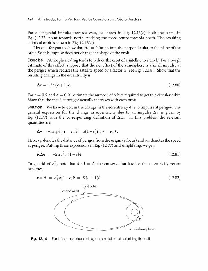
474 An Introduction to Vectors, Vector Operators and Vector Analysis
For a tangential impulse towards west, as shown in Fig. 12.13(c), both the terms inEq. (12.77) point towards north, pushing the force centre towards north. The resultingelliptical orbit is shown in Fig. 12.13(d).
I leave it for you to show that ∆e = 0 for an impulse perpendicular to the plane of theorbit. So this impulse does not change the shape of the orbit.
Exercise Atmospheric drag tends to reduce the orbit of a satellite to a circle. For a roughestimate of this effect, suppose that the net effect of the atmosphere is a small impulse atthe perigee which reduces the satellite speed by a factor α (see Fig. 12.14 ). Show that theresulting change in the eccentricity is
∆e = −2α(e+ 1)e. (12.80)
For e = 0.9 and α = 0.01 estimate the number of orbits required to get to a circular orbit.Show that the speed at perigee actually increases with each orbit.
Solution We have to obtain the change in the eccentricity due to impulse at perigee. Thegeneral expression for the change in eccentricity due to an impulse ∆v is given byEq. (12.77) with the corresponding definition of ∆H. In this problem the relevantquantities are,
∆v = −αv+v ; r = r+r = a(1− e)r ; v = v+v.
Here, r+ denotes the distance of perigee from the origin (a focus) and v+ denotes the speedat perigee. Putting these expressions in Eq. (12.77) and simplifying, we get,
K∆e = −2αv2+a(1− e)e. (12.81)
To get rid of v2+, note that for r = e, the conservation law for the eccentricity vector
becomes,
v×H = v2+a(1− e)e = K(e+ 1)e. (12.82)
Fig. 12.14 Earth’s atmospheric drag on a satellite circularising its orbit
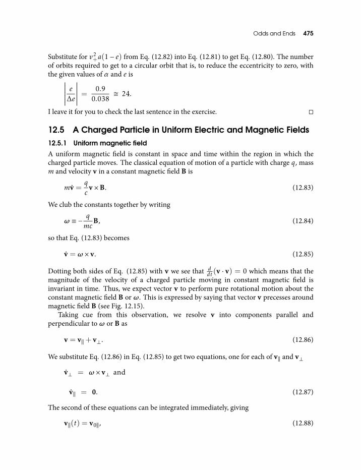
Odds and Ends 475
Substitute for v2+a(1− e) from Eq. (12.82) into Eq. (12.81) to get Eq. (12.80). The number
of orbits required to get to a circular orbit that is, to reduce the eccentricity to zero, withthe given values of α and e is∣∣∣∣∣∣∣ e∆e
∣∣∣∣∣∣∣ = 0.90.038
24.
I leave it for you to check the last sentence in the exercise.
12.5 A Charged Particle in Uniform Electric and Magnetic Fields12.5.1 Uniform magnetic field
A uniform magnetic field is constant in space and time within the region in which thecharged particle moves. The classical equation of motion of a particle with charge q, massm and velocity v in a constant magnetic field B is
mv =q
cv×B. (12.83)
We club the constants together by writing
ω ≡ −q
mcB, (12.84)
so that Eq. (12.83) becomes
v = ω × v. (12.85)
Dotting both sides of Eq. (12.85) with v we see that ddt (v · v) = 0 which means that the
magnitude of the velocity of a charged particle moving in constant magnetic field isinvariant in time. Thus, we expect vector v to perform pure rotational motion about theconstant magnetic field B or ω. This is expressed by saying that vector v precesses aroundmagnetic field B (see Fig. 12.15).
Taking cue from this observation, we resolve v into components parallel andperpendicular to ω or B as
v = v‖+ v⊥. (12.86)
We substitute Eq. (12.86) in Eq. (12.85) to get two equations, one for each of v‖ and v⊥
v⊥ = ω × v⊥ and
v‖ = 0. (12.87)
The second of these equations can be integrated immediately, giving
v‖(t) = v0‖, (12.88)
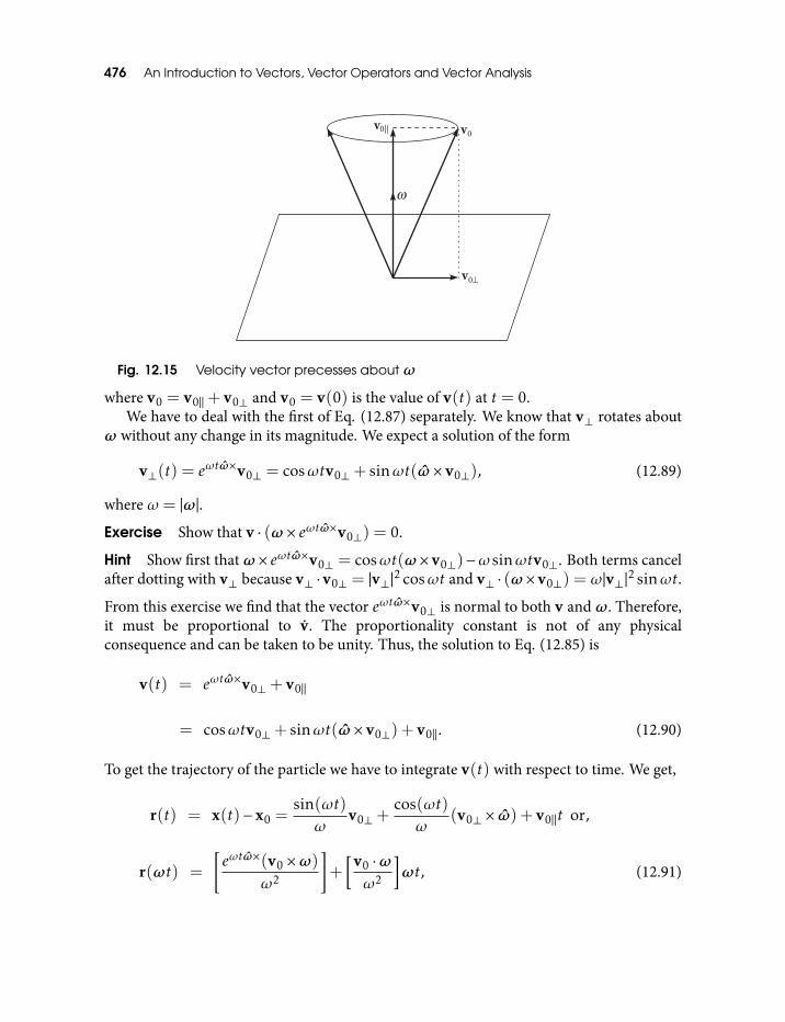
476 An Introduction to Vectors, Vector Operators and Vector Analysis
Fig. 12.15 Velocity vector precesses about ω
where v0 = v0‖+ v0⊥ and v0 = v(0) is the value of v(t) at t = 0.We have to deal with the first of Eq. (12.87) separately. We know that v⊥ rotates about
ω without any change in its magnitude. We expect a solution of the form
v⊥(t) = eωtω×v0⊥ = cosωtv0⊥+ sinωt(ω × v0⊥), (12.89)
where ω = |ω|.
Exercise Show that v · (ω × eωtω×v0⊥) = 0.
Hint Show first that ω × eωtω×v0⊥ = cosωt(ω ×v0⊥)−ω sinωtv0⊥. Both terms cancelafter dotting with v⊥ because v⊥ ·v0⊥ = |v⊥|2 cosωt and v⊥ · (ω ×v0⊥) = ω|v⊥|2 sinωt.
From this exercise we find that the vector eωtω×v0⊥ is normal to both v and ω. Therefore,it must be proportional to v. The proportionality constant is not of any physicalconsequence and can be taken to be unity. Thus, the solution to Eq. (12.85) is
v(t) = eωtω×v0⊥+ v0‖
= cosωtv0⊥+ sinωt(ω × v0⊥) + v0‖. (12.90)
To get the trajectory of the particle we have to integrate v(t) with respect to time. We get,
r(t) = x(t)− x0 =sin(ωt)ω
v0⊥+cos(ωt)ω
(v0⊥ × ω) + v0‖t or,
r(ωt) =
[eωtω×(v0 ×ω)
ω2
]+
[v0 ·ωω2
]ωt, (12.91)
Odds and Ends 477
where x0 is the constant of integration, so that the state of the particle at t = 0 is givenby (x0,v0). We have also used (ω × v0‖) = 0, and v0‖ = v0 · ωω. Equation (12.91) is acoordinate free equation of an helix (see Fig. 12.16) with radius
a ≡(v0 ×ω)ω2
and pitch
b ≡ v0 ·ωω2 .
We can make Eq. (12.91) look like a helix by expressing it in terms of
θ = θω where θ = ωt. (12.92)
Fig. 12.16 (a) Right handed helix (b) Left handed helix
In terms of these variables, Eq. (12.91) takes the form
r(θ) = eθθ×a+ bθ (12.93)
where a ·θ = 0. The helix is said to be right handed if b > 0 and left handed if b < 0 (seeFig. 12.16).
Equation (12.91) gives a circular trajectory if v0‖ = 0. The radius vector r rotates withan angular speed ω = |qB|/mc called the cyclotron frequency . Equation (12.84) tells usthat ω has the same (opposite) direction as the magnetic field B when the charge q isnegative (positive). As shown in Fig. 12.17, the circular motion of a negative (positive)charge is right handed (left handed).
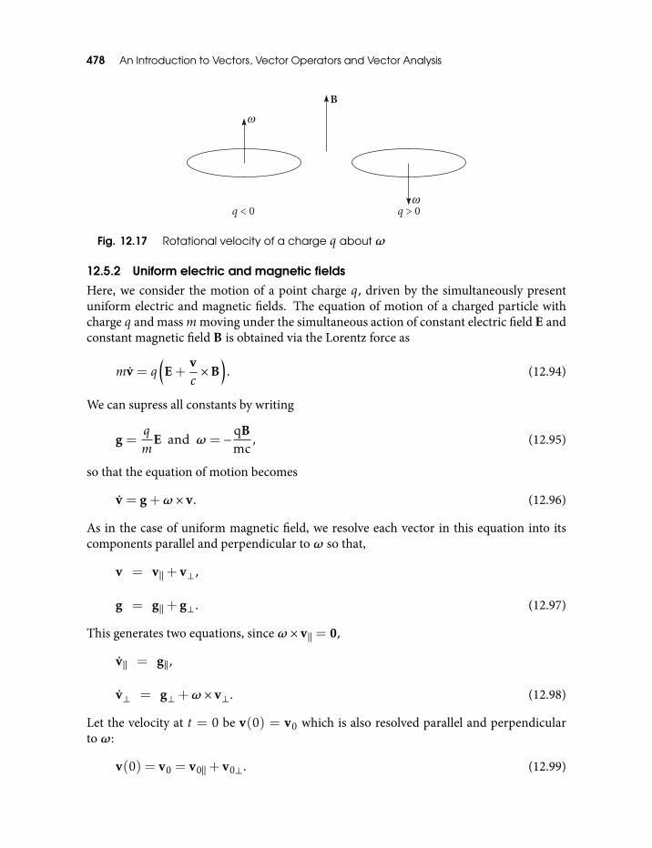
478 An Introduction to Vectors, Vector Operators and Vector Analysis
Fig. 12.17 Rotational velocity of a charge q about ω
12.5.2 Uniform electric and magnetic fields
Here, we consider the motion of a point charge q, driven by the simultaneously presentuniform electric and magnetic fields. The equation of motion of a charged particle withcharge q and massmmoving under the simultaneous action of constant electric field E andconstant magnetic field B is obtained via the Lorentz force as
mv = q(E+
vc×B
). (12.94)
We can supress all constants by writing
g =q
mE and ω = −qB
mc, (12.95)
so that the equation of motion becomes
v = g+ω × v. (12.96)
As in the case of uniform magnetic field, we resolve each vector in this equation into itscomponents parallel and perpendicular to ω so that,
v = v‖+ v⊥,
g = g‖+ g⊥. (12.97)
This generates two equations, since ω × v‖ = 0,
v‖ = g‖,
v⊥ = g⊥+ω × v⊥. (12.98)
Let the velocity at t = 0 be v(0) = v0 which is also resolved parallel and perpendicularto ω:
v(0) = v0 = v0‖+ v0⊥. (12.99)
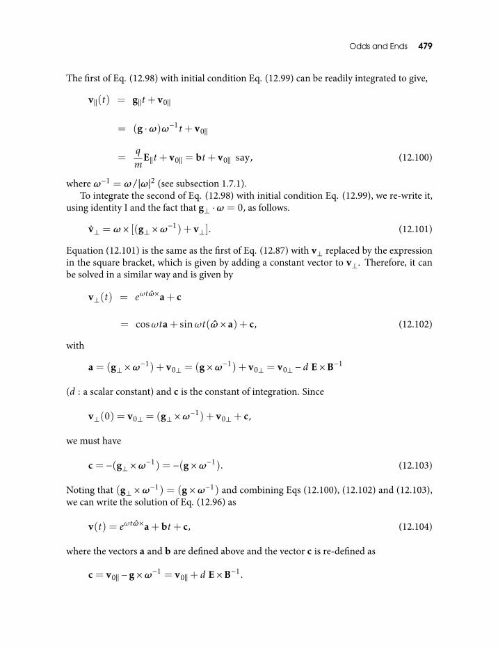
Odds and Ends 479
The first of Eq. (12.98) with initial condition Eq. (12.99) can be readily integrated to give,
v‖(t) = g‖t+ v0‖
= (g ·ω)ω−1t+ v0‖
=q
mE‖t+ v0‖ = bt+ v0‖ say, (12.100)
where ω−1 = ω/|ω|2 (see subsection 1.7.1).To integrate the second of Eq. (12.98) with initial condition Eq. (12.99), we re-write it,
using identity I and the fact that g⊥ ·ω = 0, as follows.
v⊥ = ω × [(g⊥ ×ω−1) + v⊥]. (12.101)
Equation (12.101) is the same as the first of Eq. (12.87) with v⊥ replaced by the expressionin the square bracket, which is given by adding a constant vector to v⊥. Therefore, it canbe solved in a similar way and is given by
v⊥(t) = eωtω×a+ c
= cosωta+ sinωt(ω × a) + c, (12.102)
with
a = (g⊥ ×ω−1) + v0⊥ = (g×ω−1) + v0⊥ = v0⊥ − d E×B−1
(d : a scalar constant) and c is the constant of integration. Since
v⊥(0) = v0⊥ = (g⊥ ×ω−1) + v0⊥+ c,
we must have
c = −(g⊥ ×ω−1) = −(g×ω−1). (12.103)
Noting that (g⊥ ×ω−1) = (g×ω−1) and combining Eqs (12.100), (12.102) and (12.103),we can write the solution of Eq. (12.96) as
v(t) = eωtω×a+bt+ c, (12.104)
where the vectors a and b are defined above and the vector c is re-defined as
c = v0‖ − g×ω−1 = v0‖+ d E×B−1.
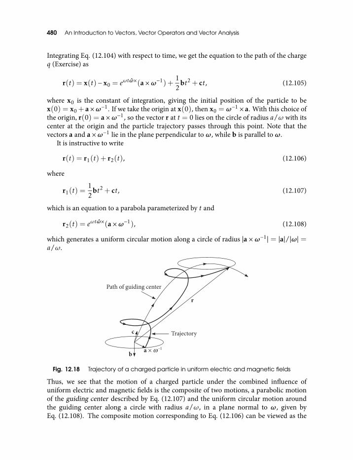
480 An Introduction to Vectors, Vector Operators and Vector Analysis
Integrating Eq. (12.104) with respect to time, we get the equation to the path of the chargeq (Exercise) as
r(t) = x(t)− x0 = eωtω×(a×ω−1) +12
bt2 + ct, (12.105)
where x0 is the constant of integration, giving the initial position of the particle to bex(0) = x0 + a×ω−1. If we take the origin at x(0), then x0 = ω−1 ×a. With this choice ofthe origin, r(0) = a×ω−1, so the vector r at t = 0 lies on the circle of radius a/ω with itscenter at the origin and the particle trajectory passes through this point. Note that thevectors a and a×ω−1 lie in the plane perpendicular to ω, while b is parallel to ω.
It is instructive to write
r(t) = r1(t) + r2(t), (12.106)
where
r1(t) =12
bt2 + ct, (12.107)
which is an equation to a parabola parameterized by t and
r2(t) = eωtω×(a×ω−1), (12.108)
which generates a uniform circular motion along a circle of radius |a ×ω−1| = |a|/|ω| =a/ω.
Fig. 12.18 Trajectory of a charged particle in uniform electric and magnetic fields
Thus, we see that the motion of a charged particle under the combined influence ofuniform electric and magnetic fields is the composite of two motions, a parabolic motionof the guiding center described by Eq. (12.107) and the uniform circular motion aroundthe guiding center along a circle with radius a/ω, in a plane normal to ω, given byEq. (12.108). The composite motion corresponding to Eq. (12.106) can be viewed as the
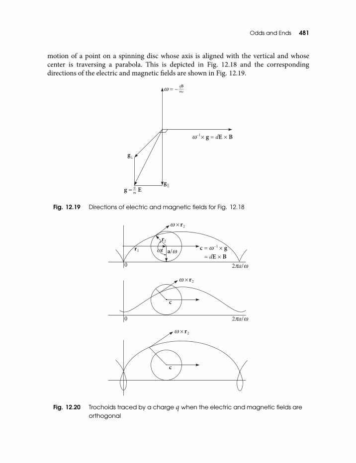
Odds and Ends 481
motion of a point on a spinning disc whose axis is aligned with the vertical and whosecenter is traversing a parabola. This is depicted in Fig. 12.18 and the correspondingdirections of the electric and magnetic fields are shown in Fig. 12.19.
Fig. 12.19 Directions of electric and magnetic fields for Fig. 12.18
Fig. 12.20 Trochoids traced by a charge q when the electric and magnetic fields areorthogonal
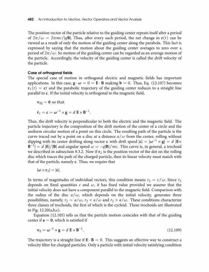
482 An Introduction to Vectors, Vector Operators and Vector Analysis
The position vector of the particle relative to the guiding center repeats itself after a periodof 2π/ω = 2πmc/|qB|. Thus, after every such period, the net change in r(t) can beviewed as a result of only the motion of the guiding center along the parabola. This fact isexpressed by saying that the motion about the guiding center averages to zero over aperiod of 2π/ω. So motion of the guiding center can be regarded as an average motion ofthe particle. Accordingly, the velocity of the guiding center is called the drift velocity ofthe particle.
Case of orthogonal fieldsThe special case of motion in orthogonal electric and magnetic fields has importantapplications. In this case, g ·ω = 0 = E ·B making b = 0. Thus, Eq. (12.107) becomesr1(t) = ct and the parabolic trajectory of the guiding center reduces to a straight lineparallel to c. If the initial velocity is orthogonal to the magnetic field,
v0‖ = 0 so that
r1 = c = ω−1 × g = d E×B−1.
Thus, the drift velocity is perpendicular to both the electric and the magnetic field. Theparticle trajectory is the composition of the drift motion of the center of a circle and theuniform circular motion of a point on this circle. The resulting path of the particle is thecurve traced out by a point on a disc at a distance a/ω from the center, rolling withoutslipping with its center drifting along vector c with drift speed |c| = |ω−1 × g| = d |E×B−1| = d |E|/|B| and angular speed ω = −q|B|/mc. This curve is, in general, a trochoidwe described in subsection 9.3.2. Now if r2 is the position vector of the dot on the rollingdisc which traces the path of the charged particle, then its linear velocity must match withthat of the particle, namely c. Thus, we require that
|ω × r2|= |c|.
In terms of magnitudes of individual vectors, this condition means r2 = c/ω. Since r2depends on fixed quantities c and ω, it has fixed value provided we assume that theinitial velocity does not have a component parallel to the magnetic field. Comparison withthe radius of the disc a/ω, which depends on the initial velocity, generates threepossibilities, namely, r2 = a/ω, r2 < a/ω and r2 > a/ω. These conditions characterizethree classes of trochoids, the first of which is the cycloid. These trochoids are illustratedin Fig. 12.20(a,b,c).
Equation (12.105) tells us that the particle motion coincides with that of the guidingcenter if a = 0, which is satisfied if
v0 = ω−1 × g = d E×B−1. (12.109)
The trajectory is a straight line if E ·B = 0. This suggests an effective way to construct avelocity filter for charged particles. Only a particle with initial velocity satisfying condition
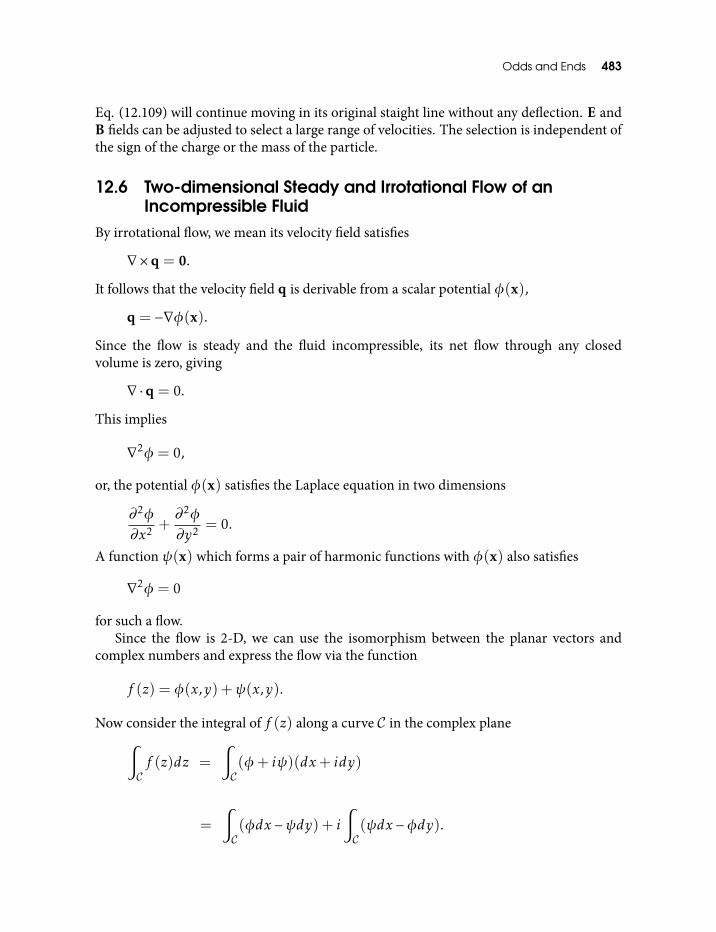
Odds and Ends 483
Eq. (12.109) will continue moving in its original staight line without any deflection. E andB fields can be adjusted to select a large range of velocities. The selection is independent ofthe sign of the charge or the mass of the particle.
12.6 Two-dimensional Steady and Irrotational Flow of anIncompressible Fluid
By irrotational flow, we mean its velocity field satisfies
∇×q = 0.
It follows that the velocity field q is derivable from a scalar potential φ(x),
q = −∇φ(x).
Since the flow is steady and the fluid incompressible, its net flow through any closedvolume is zero, giving
∇ ·q = 0.
This implies
∇2φ = 0,
or, the potential φ(x) satisfies the Laplace equation in two dimensions
∂2φ
∂x2 +∂2φ
∂y2 = 0.
A function ψ(x) which forms a pair of harmonic functions with φ(x) also satisfies
∇2φ = 0
for such a flow.Since the flow is 2-D, we can use the isomorphism between the planar vectors and
complex numbers and express the flow via the function
f (z) = φ(x,y) +ψ(x,y).
Now consider the integral of f (z) along a curve C in the complex plane∫Cf (z)dz =
∫C(φ+ iψ)(dx+ idy)
=
∫C(φdx −ψdy) + i
∫C(ψdx −φdy).
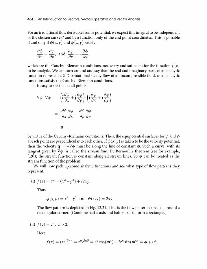
484 An Introduction to Vectors, Vector Operators and Vector Analysis
For an irrotational flow derivable from a potential, we expect this integral to be independentof the chosen curve C and be a function only of the end point coordinates. This is possibleif and only if φ(x,y) and ψ(x,y) satisfy
∂φ
∂x=∂ψ
∂y, and
∂ψ
∂x= −
∂φ
∂y,
which are the Cauchy–Riemann conditions, necessary and sufficient for the function f (z)to be analytic. We can turn around and say that the real and imaginary parts of an analyticfunction represent a 2-D irrotational steady flow of an incompressible fluid, as all analyticfunctions satisfy the Cauchy–Riemann conditions.
It is easy to see that at all points
∇φ · ∇ψ =
(i∂φ
∂x+ j
∂φ
∂y
)·(i∂ψ
∂x+ j
∂ψ
∂y
)
=∂φ
∂x
∂ψ
∂x+∂φ
∂y
∂ψ
∂y
= 0
by virtue of the Cauchy–Riemann conditions. Thus, the equipotential surfaces for φ and ψat each point are perpendicular to each other. Ifφ(x,y) is taken to be the velocity potential,then the velocity q = −∇φ must be along the line of constant ψ. Such a curve, with itstangent given by ∇φ, is called the stream line. By Bernoulli’s theorem (see for example,[19]), the stream function is constant along all stream lines. So ψ can be treated as thestream function of the problem.
We will now pick up some analytic functions and see what type of flow patterns theyrepresent.
(i) f (z) = z2 = (x2 − y2) + i2xy.
Thus,
φ(x,y) = x2 − y2 and ψ(x,y) = 2xy.
The flow pattern is depicted in Fig. 12.21. This is the flow pattern expected around arectangular corner. (Combine half x axis and half y axis to form a rectangle.)
(ii) f (z) = zn, n > 2.
Here,
f (z) = (reiθ)n = rneinθ = rn cos(nθ) + irn sin(nθ) = φ+ iψ.
Odds and Ends 485
Fig. 12.21 Two-dimensional flow around a 90 corner
This corresponds to a flow pattern around an angle α = π/n. The case with n = 3is shown in Fig. 12.22.
Fig. 12.22 Two-dimensional flow around a 60 corner
(iii) f (z) = A√z,
A being a real constant. Here,
φ(x,y) = A√r cos(θ/2) and ψ(x,y) = A
√rsin(θ/2).
This gives
2φ2
A2 = 2r cos2(θ/2) = r(1+ cosθ) = r + x
and
2ψ2
A2 = 2r sin2(θ/2) = r(1− cosθ) = r − x.
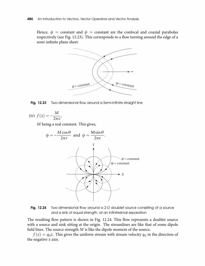
486 An Introduction to Vectors, Vector Operators and Vector Analysis
Hence, φ = constant and ψ = constant are the confocal and coaxial parabolasrespectively (see Fig. 12.23). This corresponds to a flow turning around the edge of asemi-infinite plane sheet.
Fig. 12.23 Two-dimensional flow around a Semi-infinite straight line
(iv) f (z) = − M2πz
,
M being a real constant. This gives,
φ = −M cosθ2πr
and ψ =Msinθ
2πr.
Fig. 12.24 Two-dimensional flow around a 2-D doublet source consisting of a sourceand a sink of equal strength, at an infinitesimal separation
The resulting flow pattern is shown in Fig. 12.24. This flow represents a doublet sourcewith a source and sink sitting at the origin. The streamlines are like that of some dipolefield lines. The source strengthM is like the dipole moment of the source.f (z) = q0z. This gives the uniform stream with stream velocity q0 in the direction of
the negative x axis.
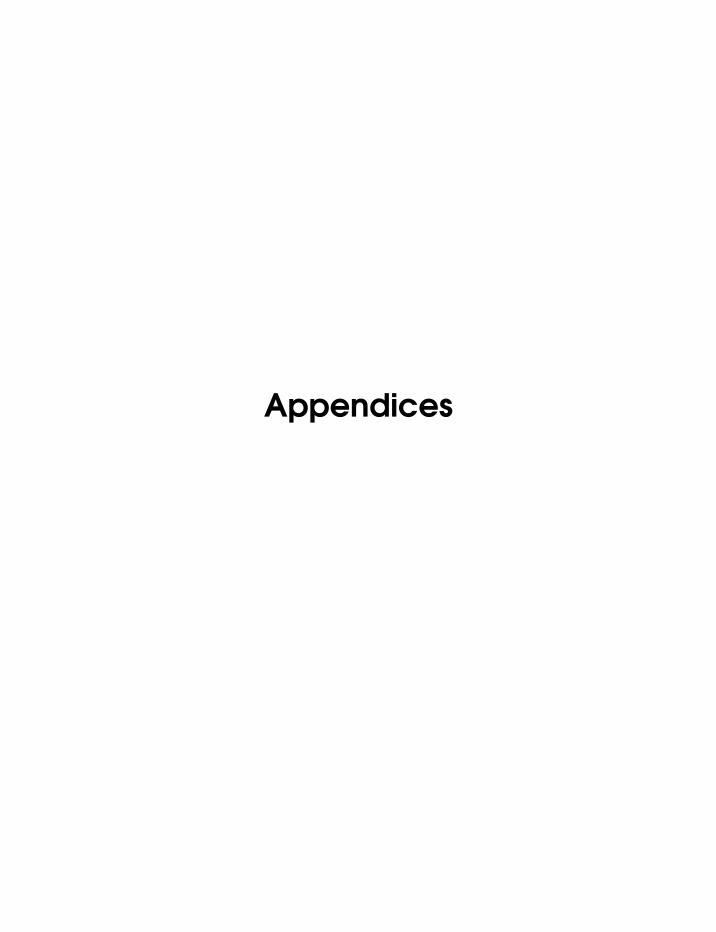
Appendices

A
Matrices and Determinants
In this appendix we develop the theory of matrices and determinants, as required by thisbook, emphasizing their connection with vectors. This approach is not coordinate-free: Wehave to represent vectors by their coordinates with respect to some basis. This approach hasthe advantage of being easily generalizable to higher dimensional spaces. Our interest inmatrices and determinants stems from their role in understanding of and computationswith linear operators and their connection with the orientations of triplets of vectors andof surfaces. In the course of this appendix we may re-derive some of the results we haveobtained in the text. Of course, this appendix can be used to explain all instances wherewe have used matrices and/or determinants. Theory of matrices is an independent, fullydeveloped branch of mathematics worthy of an independent, rewarding and fruitful study.We recommend [12] for such a study.
A.1 Matrices and Operations on themA matrix is the arrangement of m× n real or complex numbers in m rows and n columns.In this book, we deal with real matrices with m,n ≤ 3, although in this appendix we dealwith a general m × n real matrix. The pair (m,n) defines the size of a matrix. We usecapital letters to denote a matrix, thus a matrix with m rows and n columns is denotedAm×n or just A if the suffix m × n can be left understood. An element in the ith row andjth column in A is denoted aij and the matrix is written
A= [aij ] i = 1, . . . ,m ; j = 1, . . . ,n.
On most occasions the ranges of the subscripts i and j are left understood.By fixing an orthonormal basis in En we have the isomorphism
x ∈ En↔
x1x2...xn
∈Mn×1, (A.1)
490 Appendices
whereMn×1 is the space of n×1 matrices called column vectors. For an orthonormal basisek k = 1, . . . ,n in En we have the correspondence
ek↔
00...1...0
; k = 1, . . . ,n (A.2)
where for ek , 1 occurs in the kth row. The transpose of a vector x is defined by xT =(x1 x2 . . . xn). The transpose of a column vector is the corresponding row vector. Both thecolumn vectors representing ek, k = 1, . . . ,n and the row vectors representing eTk , k =1, . . . ,n are called “coordinate vectors”.
Exercise Show that the set of all m × n real matrices forms a linear space of dimensionmn.
Hint Show that this set is isomorphic with the space of allmn-tuples, namely Rmn.
The rows of am×nmatrixA can be identified with the vectors a1,a2, . . . ,am as the vectorsin Rn,
ak = (ak1,ak2, . . . ,akn) ; k = 1,2, . . . ,m.
The matrix A can be written as
A=
a1
a2...
am
. (A.3)
Given an n dimensional vector x and am dimensional vector y,
x↔
x1...xn
and y↔
y1...ym
, (A.4)
the equation
Ax = y (A.5)
Appendices 491
stands for a system of equations
a11x1 + a12x2 + · · ·+ a1nxn = y1
a21x1 + a22x2 + · · ·+ a2nxn = y2
...
am1x1 + am2x2 + · · ·+ amnxn = ym (A.6)
The system of simultaneous equations, (Eq. (A.6)), can be written as
x1
a11
a21
...
am1
+ x2
a12
a22
...
am2
+ · · ·+ xn
a1n
a2n
...
amn
=
y1
y2
...
ym
. (A.7)
Viewed as the system of simultaneous equations, Eq. (A.5) connects the components(x1, . . . ,xn) of the vector x with respect to the basis of vectors defined in the last equationin an n-dimensional subspace to the components of the same vector (y1, . . . ,ym) withrespect to the basis ek ; k = 1, . . . ,m. Thus, in this case Eq. (A.5) becomes a passivetransformation transforming the components of the same vector from one basis to theother.
We can also view Eq. (A.5) as an active transformation or as a map or a linear operatorA : En 7→ Em mapping vectors x ∈ En to vectors y ∈ Em. If we shift the origin by a constantvector b then Eq. (A.5) becomes
y = Ax+b (A.8)
Equation (A.8) defines an affine transformation. This is the most general result of the actionof a matrix on a vector.
As an example, the matrix
A=
23 −1
3
−13
23
−13 −1
3
(A.9)
can be actively interpreted as a mapping of vectors x = (x1x2) in the (x1x2) plane ontothe vectors y = (y1,y2,y3) in the plane defined by
y1 + y2 + y3 = 0
492 Appendices
which is perpendicular to the vector N = (1,1,1) and which we call π. Geometrically, thepoint (y1,y2,y3) is obtained by projecting the point (x1x2,0) perpendicularly to the planeπ. Alternatively, the corresponding system of equations
y1 =23x1 −
13x2; y2 = −
13x1 +
23x2; y3 = −
13x1 −
13x2
can be interpreted passively as a parametric representation of the plane π, with x1,x2 asparameters.
Given a scalar λ we have,
λA= [λaij ] ; i = 1, . . . ,m ; j = 1, . . . ,n.
Two matrices of the same size can be added. The ijth element of the matrix obtained byadding A and B is the addition of the ijth elements of the matrices A and B :
A+B= [aij + bij ]
C = A+B implies cij = aij + bij . Thus, we can construct a linear combination∑k λkAk
whereAk k = 1, . . . are the matrices of the same size saym×n and λk are scalars. Additionof matrices is associative, (A+B)+C = A+(B+C) and commutative,A+B= B+A. Itis distributive with respect to the multiplication by a scalar. That is, λ(A+B) = λA+λBand (α+ β)A= αA+ βA, α,β,λ being scalars.
Two matrices can be multiplied provided the number of columns of the left multiplierequals the number of rows of the right multiplier. Then the ijth element of the product is
cij =∑k
aikbkj .
That is, the ith row of A is is elementwise multiplied with the jth column of B and thecorresponding products are summed over, to get the ijth element of the product C = AB.Note that, in general, AB , BA, that is, matrix product is not commutative. In fact onlyone of the products AB or BAmay be defined while the other may not.
Product of matrices can be understood via the composition of mappings. If y = Axis the map A : Em 7→ En defined by the matrix An×m = [aji ] then by linearity, as shownabove, its explicit form is
yj =m∑i=1
ajixi .
Now suppose Bp×n = [bkj ] defines a map z = By, En 7→ Ep, then the vector z is given by
zk =n∑j=1
bkjyj =n∑j=1
m∑i=1
bkjajixi =m∑i=1
ckixi ,
Appendices 493
where
cki =n∑j=1
bkjaji ; k = 1, . . . ,p; i = 1, . . . ,m.
Thus, z = Cx where C = BA = [cki ] is the matrix with p rows and m columns defined bythe last equation. Accordingly, we take the matrix C defined above to be the product BA ofmatrices A and B in that order.
The matrix product is associative and distributive with respect to matrix addition. Thus,for three matrices A,B,C with appropriate sizes,
(AB)C = A(BC)
and
A(B+C) = AB+AC.
Note that, in the last equation, matrices B and C must be of the same size, so if the productAB is defined, so is AC. The last equation is valid with multiplication in the reverse order.For the mappings of vectors determined by matrices, we can write
(A+B)x = Ax+Bx; (λA)x = λ(Ax); A(B+C)x = ABx+ACx.
From the definition of the scalar product of two vectors in terms of their coordinates, wesee that x ·y = xT y where x and y are the column vectors (n×1 matrices) representing thevectors x and y. For an orthonormal basis ek, k = 1, . . . ,n we have
eTi · ek = [0 0 · · · 1 · · · 0]
00...1...0
=
0 for i , k,1 for i = k.
(A.10)
where 1 is at ith place in the left multiplier and at kth place in the right multiplier. Thus,coordinate vectors are orthonormal, as they should be. In general, for any two orthogonalvectors, we have,
x · y = xT y = 0.
We end this subsection by defining the transpose of a matrix. The transpose of a m × nmatrix A is the n ×m matrix AT obtained by interchanging the rows and columns of A.Thus, the ijth element ofAT , denoted aTij is the same as the jith element ofA giving us thedefining equation
494 Appendices
aTij = aji .
The transpose AT of a n×n square matrix A is also a n×n square matrix.
A.2 Square Matrices, Inverse of a Matrix, Orthogonal MatricesSquare matrices are those having equal number of rows and columns and are extremelyimportant in applications. The order of a square matrix is the number of rows or columns.Any two square matrices of the same order n can be added or multiplied. We can formpowers of such a matrix
A2AA, A3 = AAA, · · · .
The zero matrix O of order n is the matrix all of whose elements are zero. All the rows(columns) of zero matrix are zero vectors 0 = (0,0, . . . ,0)T of n dimensional space. It hasthe obvious properties
A+O = A=O+A, AO =OA=O
for all nth order matrices A and
Ox =O for all x ∈ En.
The unit matrix of order n, denoted I is the matrix representing the identity mapping
Ix = x for all x ∈ En.
In particular, for any orthonormal basis in En we must have
I ek = ek k = 1,2, . . . ,n,
from which we can conclude that the column (row) vectors in I are given by the coordinatevectors as in Eq. (A.2).
I = (e1, e2, · · · , en) =
1 0 0 · · · 00 1 0 · · · 0...
......
...0 0 0 · · · 1
· (A.11)
The nth order unit matrix I is the multiplicative identity for matrix multiplication. That is,
IA= AI = A
for all nth order matrices A.
Appendices 495
Given a nth order matrix A, the matrix A−1 satisfying
A−1A= I = AA−1
is called the inverse ofA. A nth order matrixA for whichA−1 exists is called invertible. Westate and prove the following properties of a nth order invertible matrix.
(i) The inverse of a nth order invertible matrix A is unique.Proof If possible, let B and C be two distinct inverses of A satisfying AB = BA =I = AC. Then we have,
B−C = BA(B−C) = B(AB−AC) = BO =O
so that B= C.
(ii) A nth order matrix A is invertible if and only if Ax = 0 implies x = 0, or, if and onlyif x , 0 implies Ax , 0.
Proof (if part). We are given that Ax = 0 implies x = 0. We show that thecorresponding map A : En 7→ En is both one to one and onto and hence invertible. Ifpossible, let x1 , x2 with Ax1 = Ax2. This means, by linearity of A thatA(x1 − x2) = 0 so that A maps a non-zero vector x1 − x2 to the zero vector,contradicting the axiom. Therefore, Ax1 = Ax2 implies x1 = x2 or, in other words,A is one to one. Since the images of two distinct vectors in En under the map A aredistinct, and since the map A is defined for all vectors in En, the image set of Acoincides with its domain En or, in other words, A is onto. Therefore, the inverse ofthe map A exists and the corresponding matrix is the inverse of the matrix A.
(only if part). We are given that A is invertible. Then Ax = 0 =⇒ A−1Ax =0 =⇒ x = 0. A matrix mapping a non-zero vector to the zero vector is calledsingular. Thus, a matrix is invertible if and only if it is non-singular
(iii) A nth order matrix A is invertible if and only if its determinant is not zero.Proof (if part) The determinant of a square matrix is the product of its eigenvalues.If the determinant is zero, then at least one of the eigenvalues of A is zero. Since theeigenvector is non-zero, the corresponding eigenvalue equation reads Ax = 0x = 0,so that A maps a non-zero vector to the zero vector and hence must not beinvertible. Alternatively, if det(A) , 0, the system AX = Y has unique solutionBY = X. Substituting, these two equations into each other we get AB = I = BAwhich means B= A−1.
(only if part) We are given that A is invertible. Therefore, A−1A = I so thatdet(A−1A) = det(A−1)det(A) = det(I) = 1 which means det(A) , 0.
(iv) A nth order matrix A is invertible if and only if it maps every basis to some basis.Proof (if part) We are given that Amaps a linearly independent set x1,x2, . . . ,xn tothe linearly independent set Ax1,Ax2, . . . ,Axn. Consider x =
∑nk=1 akxk such that
496 Appendices
Ax =∑nk=1 akAxk = 0. Since Axk; k = 1, . . . ,n are linearly independent, this
equation is satisfied only when all aks are zero, in which case x =∑nk=1 akxk = 0.
Thus, Ax = 0 implies x = 0 or A is invertible.
(only if part) We are given that A is invertible, so that Ax =∑nk=1 akAxk = 0
implies x =∑nk=1 akxk = 0. Since xk is a basis, the last equation makes all aks
zero, which means, via the previous equation, that the set Ax1,Ax2, . . . ,Axn islinearly independent.
(v) A nth order matrix A is invertible if and only if the column vectors of A are linearlyindependent.
Proof From Eq. (A.7) it is clear that Ax = 0 for x , 0 if and only if the columnvectors of A are linearly dependent.
Exercise Show that a matrix is singular if and only if its determinant vanishes.
We have defined and used orthogonal matrices in connection with the rotation of a vectorabout a direction in space. The orthogonal matrices correspond to linear operators ortransformations that preserve length or distance between points in space. If two pointsP ,Q in space with coordinates (xi ,yi), i = 1, . . . ,n go over to points P ′,Q′, withcoordinates (x′i ,y
′i ), i = 1, . . . ,n under an orthogonal transformation defined by the
orthogonal matrix R= [aij ], then we require that
d2(P ,Q) =n∑i=1
(xi − yi)2 =n∑i=1
(x′i − y′i )
2 = d2(P ′,Q′). (A.12)
Putting x′i =∑j aijxj and y′i =
∑k aikxk in Eq. (A.12) you can check that Eq. (A.12) is
satisfied provided
n∑i=1
aijaik = δjk , (A.13)
where δjk is the Kronaker delta, which is zero when j , k and is 1 if j = k, or,
aj · ak = δjk . (A.14)
That is, the jth and the kth column vectors of R are orthonornal. Since a set of orthogonalvectors is essentially linearly independent, the n column vectors of R form an orthonormalbasis of the n dimensional space. Thus, every orthogonal matrix is invertible, by virtue of(v) above. In fact Eq. (A.13) can be written as
n∑i=1
aTjiaik = δik ,
Appendices 497
or,
RTR= I = RRT . (A.15)
Thus, the transpose of an orthogonal matrix equals its inverse.More generally, the orthogonal transformation preserves the scalar product:
Rx ·Ry = x · y. (A.16)
Exercise Show that an orthogonal matrix Rmust have det(R) = ±1.
Solution We have, det(RTR) = det(RT )det(R) = (det(R))2 = det(I) = 1 whichgives det(R) = ±1.
The set of orthogonal 3×3 matrices with det(R) = +1 represents all possible rotations in3-D Euclidean space. This result is due to Euler (see section 6.6). In fact, thecorrespondence between the the rotations and orthogonal matrices with det(R) = +1 isan isomorphism:
R1 R2 =R =⇒ [R1] [R2] = [R],
where [R1], [R2] and [R] represent the corresponding rotations.The passive and active interpretations of the orthogonal transformations are described
in the text (see section 6.4).
A.3 Linear and Multilinear Forms of VectorsOur next task in this appendix is to define determinants and formulate their principalproperties. We need some general albraic notions to do this job.
A function f (x) of vector argument x is called a linear form in x if
f (λx+ µy) = λf (x) + µf (y)
for any vectors x,y and scalars λ,µ. Thus, for example, f (x) = f (x1,x2,x3) = ax1 −
bx2 + cx3 is a linear form, while f (x) = |x| =√x2
1 + · · ·+ x2n is not. More generally, a
linear form is the one satisfying
f (λ1x1 + · · ·+λmxm) = λ1f (x1) + · · ·+λmf (xm)
valid for any m vectors x1, . . . ,xm and scalars λ1 . . . ,λm. In fact we can write any vector aas a normal form involving a basis e1, · · · , en :
a = a1e1 + · · ·+ anen ≡ (a1,a2, . . . ,an).
498 Appendices
Thus, f (a) has the form
f (a) = a1f (e1) + · · ·+ anf (en) = c1a1 + c2a2 + · · ·+ cnan,
where ci are the constant values ci = f (ei). We define the vector c ≡ (c1,c2, . . . ,cn) to get
f (a) = c · a.
Thus, the most general linear form in a vector a is the scalar product of a with with asuitable constant vector c.
A function f (x,y) of two vectors x ≡ (x1, . . . ,xn), y ≡ (y1, . . . ,yn) is called a bilinearform in x,y if f is a linear form in x for fixed y and a linear form in y for fixed x. Thus, werequire that
f (λx+ µy,z) = λf (x,z) + µf (y,z)
f (x,λy+ µz) = λf (x,y) + µf (x,z) (A.17)
for any vectors x,y,z and scalars λ,µ. The simplest example of a bilinear form is the vectorproduct
f (a,b) = a ·b.
Here, the rules Eq. (A.17) reduce to the associative and distributive laws for the scalarproduct. More generally, we find,
f (αa+ βb,γc+ δd) = αf (a,γc+ δd) + βf (b,γc+ δd)= αγf (a,c) +αδf (a,d) + βγf (b,c) + βδf (b,d).(A.18)
Thus, we can deal with the binary forms as we deal with ordinary products in multiplyingout expressions. Using the decomposition of a vector in terms of a basis e1, · · · , en, we get,for the most general bilinear form in a,b,
f (a,b) =n∑
j,k=1
ajbkf (ej , ek) =n∑
j,k=1
cjkajbk (A.19)
with constant coefficients
cjk = f (ej , ek).
For b = a, the bilinear form f goes over to the quadratic form
f (a,a) =n∑
j,k=1
cjkajak .
Appendices 499
It is now straightforward to generalize to the multilinear forms in m vectors a1,a2, . . . ,amalong with their components
a1 ≡ (a11,a21, . . . ,an1); a2 ≡ (a12,a22, . . . ,an2); . . .am ≡ (a1m,a2m, . . . ,anm).
The function f is a multilinear form f (a1,a2, . . . ,am) in a1,a2, . . . ,am if it is a linear formin each vector when the others are held fixed. We can also consider f as a function of an×mmatrix
A= [a1,a2, . . . ,am] = [ajk ],
where a1,a2, . . . ,am are its column vectors. Generalizing the bilinear case, the most generalmultilinear form in a1,a2, . . . ,am is given by
f (a1,a2, . . . ,am) =∑
j1,j2,...,jm=1,...,n
cj1j2···jmaj11aj22 · · ·ajmm (A.20)
where
cj1j2···jm = f (ej1 , ej2 , . . . , ejm).
Exercise Write explicitly Eq. (A.20) for m = 3,4,5 and n = 3. Construct explicitly then×mmatrix in each case.
A.4 Alternating Multilinear Forms: DeterminantsA function of several arguments, which could be vectors or scalars, is called alternatingif it just changes its sign as a result of interchanging any two of its arguments. Examplesof alternating functions of scalar arguments are φ(x,y) = y − x, φ(x,y,z) = (z − y)(z − x)(y − x). A function f of two n-dimensional vectors a1,a2 is alternating if
f (a1,a2) = −f (a2,a1)
for all a1,a2. This implies that
f (a,a) = 0.
Consider a 2-dimensional space and an alternating function f (a1,a2) with a1 =(a11,a21), a2 = (a12,a22). Then,
f (e1, e1) = f (e2, e2) = 0, f (e2, e1) = −f (e1, e2).
It then follows from Eq. (A.19) that
f (a1,a2) = f (a11e1 + a21e2,a12e1 + a22e2)
500 Appendices
and using the fact that f is alternating, the right side of this equation can be written
(a11a22 − a12a21)f (e1, e2) = c
∣∣∣∣∣∣a11 a12
a21 a22
∣∣∣∣∣∣= c det(a1,a2), (A.21)
where c = f (e1, e2) and we take the last equality as the definition of the determinant ofthe second order of the matrix whose columns comprise the components of vectors a1,a2.Thus, every bilinear alternating form of two vectors a1,a2 in two-dimensional space differsfrom the determinant of the matrix with columns a1,a2 by a constant factor c.
More generally, an alternating bilinear form of two vectors in n-dimensional space canbe written
f (a1,a2) =n∑
j,k=1
cjkaj1ak2,
where
cjk = −ckj , cjj = 0.
Combining the terms with subscripts which differ only by a permutation, we can express fas the linear combination of second order determinants.
f (a1,a2) =n∑
j,k=1j<k
cjk
∣∣∣∣∣∣aj1 ak1
aj2 ak2
∣∣∣∣∣∣ · (A.22)
The alternating function of three vectors, f (a1,a2,a3) changes sign whenever any twoof its arguments are exchanged. More generally, its sign is changed when the number ofexchanges of the pairs of its arguments is odd, and its sign does not change if the numberof corresponding exchanges are even. f vanishes if two of its arguments are equal.
Exercise Construct all possible permutations of the arguments a1,a2,a3 of analternating form which change its sign and which do not change its sign.
Let
a1 ≡ (a11,a21,a31), a2 ≡ (a12,a22,a32), a3 ≡ (a13,a23,a33)
be three 3-D vectors. The general alternating trilinear form f in a1,a2,a3 is
f (a1,a2,a3) =3∑
j,k,r=1
cjkraj1ak2ar3,
Appendices 501
where, using the conditions under which an alternating form changes or does not changesign and the conditions under which it vanishes, we have,
cjkr = f (ej , ek , er) = εjkrf (e1, e2, e3),
where εjkr are simply the Levi-Civita symbols which by now we know so well.
Exercise Show that εjkr = sign(φ(j,k,r)) where φ(j,k,r) = (r − k)(r − j)(k − j).
We can now write the expression for f (a1,a2,a3) explicitly using the definition of cjkr.We have,
f (a1,a2,a3) = (a11a22a33 + a12a23a31 + a13a21a32
−a13a22a31 − a11a23a32 − a12a21a33)f (e1, e2, e3) (A.23)
or,
f (a1,a2,a3) = c
∣∣∣∣∣∣∣∣∣a11 a12 a13
a21 a22 a23
a31 a32 a33
∣∣∣∣∣∣∣∣∣ , (A.24)
where c = f (e1, e2, e3) is a constant. Therefore, the most general trilinear alternating formin three 3-dimensional vectors a1,a2,a3 differs from the determinant of the matrix withcolumns a1,a2,a3 by a constant factor c. Note that
f (e1, e2, e3) = det(e1, e2, e3)f (e1, e2, e3)
so that
det(e1, e2, e3) = 1
as it should be.Generalization to higher order matrices is now straightforward. Consider a n×nmatrix
A=
a11 a12 · · · a1n
a21 a22 · · · a2n
......
...an1 an2 · · · ann
, (A.25)
with column vectors a1,a2, . . . ,an. Let f be a multilinear alternating form in a1,a2, . . . ,anas given by Eq. (A.20) where the coefficients cj1j2···jn have the form cj1j2···jn =f (ej1 , ej2 , . . . , ejn). Since f is an alternating form, these coefficients are given by
cj1j2···jn = f (ej1 , ej2 , . . . , ejn) = εj1j2···jnf (e1, e2, . . . , en),
502 Appendices
where εj1j2···jn = −1 whenever j1j2 · · · jn is obtained from 1,2, . . . ,n by odd number ofpairwise exchanges (odd permutation of 1,2, . . . ,n), εj1j2···jn = +1 whenever j1j2 · · · jnis obtained from 1,2, . . . ,n by even number of pairwise exchanges (even permutation of1,2, . . . ,n) and εj1j2···jn = 0 if any two of j1j2 · · · jn are equal. Thus, εj1j2···jn are the set ofnn symbols each with n subscripts which can be defined to be the Levi-Civita symbols withn subscripts.
Exercise Find the values of ε321, ε2143, ε4231, ε54321.
Exercise Show that εj1j2···jn = sign(φ(j1, j2, . . . , jn)) where φ(j1, j2, . . . , jn) =Πj,k=1,...,n
j<k(xk − xj).
We define the determinant of the matrix A in Eq. (A.25) as
det(A) =
∣∣∣∣∣∣∣∣∣∣∣∣∣∣
a11 a12 · · · a1n
a21 a22 · · · a2n
......
...
an1 an2 · · · ann
∣∣∣∣∣∣∣∣∣∣∣∣∣∣=
∑j1...jn
εj1j2···jnaj11aj22 . . . ajnn. (A.26)
where j1 . . . jn runs over the set of permutations of 1,2, . . . ,n (see the following exercise).
Exercise Show that there are n! terms in the expansion of an nth order determinant givenby Eq. (A.26).
Solution We have to show that there are n! non-zero values of εj1j2···jn . Since no twovalues of the subscripts can be the same, we have n choices for j1, n−1 choices for j2 . . . n−kchoices for jk . . . so that the total number of distinct εj1j2···jn are n(n−1)(n−2) · · · (n−k) · · ·1or n! which is the same as the number of terms in the required expansion. This makes thenth order determinant a nth degree form in the ajk consisting of n! terms.
Exercise Show that determinant is linear in each of its columns separately.
A.5 Principal Properties of DeterminantsEquation (A.26) gives the explicit formula for the determinant of a n×nmatrix, or the nthorder determinant, in terms of its n2 elements ajk . As shown above, this determinant isan nth degree form having n! terms. Apart from the Levi-Civita symbols, each term is aproduct of n elements one from each column and each row. Although, the expaqnsion inEq. (A.26) is explicitly computable, it has too many terms to keep track of (5! = 120 for afifth order determinant and 10! = 36,28,800 for a tenth order determinant) to be usefulfor numerical computations and more efficient ways of evaluating determinants have beendevised.
From the fact that any nth order determinant is proprtional to a n degree alternatingmultilinear form in n vectors a1,a2, . . . ,an in an n-dimensional space, we infer that for the
Appendices 503
corresponding matrix A with these vectors as its column vectors, the determinant changessign if we interchange any two of its columns. Thus, the determinant of a square matrix Achanges sign if we interchange any two columns of A; in particular, the determinant of asquare matrixAwith two identical columns vanishes. Using the linearity of the determinantin each of its columns separately, we find that multiplying one column of the matrix A by afactor λ has the effect of multiplying the determinant of A by λ. For example,
det(λa1,a2, . . . ,an) = λdet(a1,a2, . . . ,an).
In particular, for λ= 0 and arbitrary a1 we find
det(0,a2, . . . ,an) = 0,
with the same result for any other column so that the determinant of a matrix A vanishesif any column of A is the zero vector. Multiplying all elements of A by λ amounts tomultiplying every column of A by λ so that
det(λA) = λndet(A).
From the multilinearity of determinants, we conclude more generally that
det(a1+λa2,a2, . . . ,an) = det(a1,a2, . . . ,an)+λdet(a2,a2, . . . ,an) = det(a1,a2, . . . ,an)
since the matrix (a2,a2, . . . ,an) has two identical columns. Generally, the value of thedeterminant of the matrix A does not change if we add a multiple of one column to adifferent column. However, if we multiply a column by λ and add it to the same column,then the value of the determinant changes by the factor 1+λ.
We now show that the determinant of the product of two nth order matrices A and B isthe product of their determinants. To see this, note that if C = AB the resulting matrix Cis given by
C =
a1 ·b1 a1 ·b2 · · ·a1 ·bna2 ·b1 a2 ·b2 · · ·a2 ·bn
......
...an ·b1 an ·b2 · · ·an ·bn
, (A.27)
where a1,a2, . . . ,an are the row vectors of A while b1,b2, . . . ,bn are the column vectorsof B. From Eq. (A.27) we see that, keeping A fixed, det(C) is a linear form in columnvectors bk of B. Further, this is an alternating form because interchanging two columnsof B corresponds exactly to interchanging the corresponding columns ofC. Hence, det(C)is an alternating multilinear form in the column vectors of the matrix B. Consequently,
det(C) = γ det(B),
504 Appendices
where γ is the value of det(C) when bk = ek k = 1, . . . ,n or when B is the unit matrix I .Now, if B= I , then C = AB= AI = A so that γ = det(A). Thus we get,
det(AB) = det(A)det(B). (A.28)
Exercise Show that det(A−1) = 1/(det(A)).
We shall now show that a square matrixA and its transposeAT have the same determinant:
det(A) = det(AT ). (A.29)
To see this, note that in the expansion of the determinant (Eq. (A.26)) we can rearrange thefactors in each term according to the first subscripts (e.g., a31a12a23 = a12a23a31) so that,
aj11aj22 . . . ajnn = a1k1a2k2
. . . ankn . (A.30)
where k1,k2, . . . ,kn is again a perpmutation of 1,2, . . . ,n.
Exercise Show that εj1j2···jn = εk1k2···kn .
Solution We have to show that the permutations j1j2 · · · jn and k1k2 · · ·kn of 1,2, . . . ,n areeither both even or both odd. This follows from the observation that these permutationsare inverses of each other.
Equation (A.30) and the above exercise immediately lead to
det(A) =∑
k1k2...kn
εk1k2···kna1k1a2k2
. . . ankn = det(AT ).
An immediate consequence of Eq. (A.29) is that a determinant can be considered to be analternating multilinear form of its row vectors. In particular, determinant changes its sign ifwe interchange any two rows. Another consequence is that if det(A) , 0 , det(AT ) thenthe matrix AT is invertible, so that the column vectors of AT or the row vectors of A alsoform a linearly independent set.
Combining Eqs (A.28) and (A.29) we get
det(A)det(B) = det(AT )det(B) = det(ATB).
Combining this result with Eq. (A.27) we get, for the matricesA,B defined via their columnvectors, A= (a1,a2, . . . ,an) and B= (b1,b2, . . . ,bn),
det(A)det(B) = det(ATB) =
∣∣∣∣∣∣∣∣∣∣∣∣∣∣
a1 ·b1 a1 ·b2 · · ·a1 ·bna2 ·b1 a2 ·b2 · · ·a2 ·bn
......
...
an ·b1 an ·b2 · · ·an ·bn
∣∣∣∣∣∣∣∣∣∣∣∣∣∣· (A.31)
Appendices 505
A.5.1 Determinants and systems of linear equations
Determinants can be used to find whether a set of n vectors a1,a2, . . . ,an inn-dimensional space are depemdent, or, equivalently, when a square matrix A withcolumn vectors a1,a2, . . . ,an is singular. We show that a square matrix A is singular if andonly if its determinant is zero.
If A is singular, then its column vectors a1,a2, . . . ,an are linearly dependent. Thus, oneof the column vectors, say a1 can be expressed in terms of the others:
a1 = λ2a2 +λ3a3 + · · ·+λnan.
It then follows from the multilinearity of determinants that
det(A) = det(λ2a2 +λ3a3 + · · ·+λnan,a2, . . . ,an)= λ2 det(a2,a2, . . . ,an) +λ3 det(a3,a2,a3, . . . ,an) + · · ·
+λndet(an,a2,a3, . . . ,an)= 0, (A.32)
since each of the matrices has a repeated column.Conversely, if A is non-singular, it is invertible and we have
det(AA−1) = det(A)det(A−1) = det(I) = 1
so that det(A) , 0, which completes the proof.Now consider the system of equations
AX = Y
where X and Y are n × 1 column vectors and A is an n × n matrix with column vectorsa1,a2, . . . ,an. This system of equations can be re-expressed as
x1a1 + x2a2 + . . .+ xnan = y.
Then, it is straightforward to show (Exercise) that
det(a1, . . . ,ak−1,y,ak+1, . . . ,an) = xk det(a1,a2, . . . ,an), k = 1,2, . . . ,n.
If the matrix A is non-singular, we can divide by its determinant and get the solutionx1,x2, . . . ,xn expressed in terms of determinants:
x1 =det(y,a2, . . . ,an)det(a1,a2, . . . ,an)
, x2 =det(a1,y, . . . ,an)det(a1,a2, . . . ,an)
,
. . . ,xn =det(a1,a2, . . . ,y)det(a1,a2, . . . ,an)
.
This is Crammer’s rule for the solution of n linear equations in n unknowns.
506 Appendices
A.5.2 Geometrical interpretation of determinants
We start by showing how various properties of the vector product are related todeterminants. We start with the definition
det(a,b,c) =
∣∣∣∣∣∣∣∣a1 b1 c1a2 b2 c2a3 b3 c3
∣∣∣∣∣∣∣∣=∣∣∣∣∣∣∣∣a1 a2 a3b1 b2 b3c1 c2 c3
∣∣∣∣∣∣∣∣ · (A.33)
Written out as an alternating linear form in vector c we have, (see Eq. (A.23)),
det(a,b,c) = (a2b3 − a3b2)c1 + (a3b1 − a1b3)c2 + (a1b2 − a2b1)c3 = z · c,
where z ≡ (z1,z2,z3) is the vector with components
z1 = a2b3 − a3b2 =
∣∣∣∣∣a2 b2a3 b3
∣∣∣∣∣ ,z2 = a3b1 − a1b3 =
∣∣∣∣∣a3 b3a1 b1
∣∣∣∣∣ ,z3 = a1b2 − a2b1 =
∣∣∣∣∣a1 b1a2 b2
∣∣∣∣∣ ·From the components of z it is clear that z = a×b. Therefore,
det(a,b,c) = c · (a×b).
If we cyclically permute the factors on the right side, we have to interchange the columns(or rows) of the determinant on the left twice, leaving the determinant invarient. Thus,
det(a,b,c) = a · (b× c) = c · (a×b) = b · (c× a). (A.34)
The components zi of the vector z = a×b are themselves second order determinants andhence are bilinear alternating forms of vectors a,b. This immediately leads to the laws ofvector multiplication stated in the text (see Eq. (1.10)).
The property a×a = 0 follows from a×b = −b×a. More generally, the vector producttwo vectors a×b vanishes if a and b are linearly dependent, as we have seen in the text. Toprove this using determinants we note that by Eq. (A.34) a×b = 0 implies
det(a,b,c) = 0 for all vectors c,
which just means that a,b,c are dependent for all c. Since we can always choose c which islinearly independent of a,b, we conclude that a × b = 0 implies that a and b are linearlydependent or are proportional to each other.
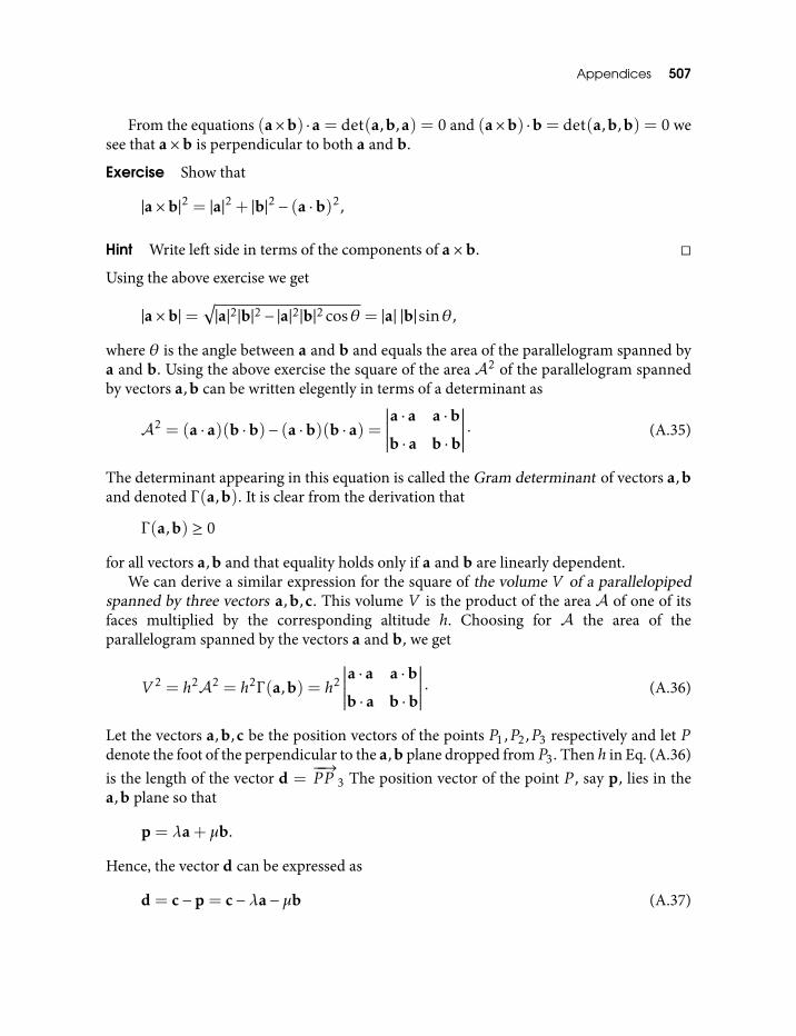
Appendices 507
From the equations (a×b) ·a = det(a,b,a) = 0 and (a×b) ·b = det(a,b,b) = 0 wesee that a×b is perpendicular to both a and b.
Exercise Show that
|a×b|2 = |a|2 + |b|2 − (a ·b)2,
Hint Write left side in terms of the components of a×b.
Using the above exercise we get
|a×b|=√|a|2|b|2 − |a|2|b|2 cosθ = |a| |b|sinθ,
where θ is the angle between a and b and equals the area of the parallelogram spanned bya and b. Using the above exercise the square of the area A2 of the parallelogram spannedby vectors a,b can be written elegently in terms of a determinant as
A2 = (a · a)(b ·b)− (a ·b)(b · a) =∣∣∣∣∣∣a · a a ·b
b · a b ·b
∣∣∣∣∣∣ · (A.35)
The determinant appearing in this equation is called the Gram determinant of vectors a,band denoted Γ (a,b). It is clear from the derivation that
Γ (a,b) ≥ 0
for all vectors a,b and that equality holds only if a and b are linearly dependent.We can derive a similar expression for the square of the volume V of a parallelopiped
spanned by three vectors a,b,c. This volume V is the product of the area A of one of itsfaces multiplied by the corresponding altitude h. Choosing for A the area of theparallelogram spanned by the vectors a and b, we get
V 2 = h2A2 = h2Γ (a,b) = h2
∣∣∣∣∣∣a · a a ·b
b · a b ·b
∣∣∣∣∣∣ · (A.36)
Let the vectors a,b,c be the position vectors of the points P1,P2,P3 respectively and let Pdenote the foot of the perpendicular to the a,b plane dropped from P3. Then h in Eq. (A.36)is the length of the vector d =
−−→P P 3 The position vector of the point P , say p, lies in the
a,b plane so that
p = λa+ µb.
Hence, the vector d can be expressed as
d = c−p = c−λa−µb (A.37)
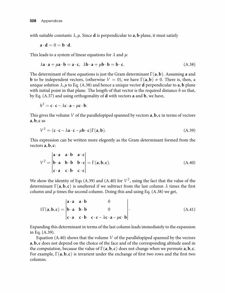
508 Appendices
with suitable constants λ,µ. Since d is perpendicular to a,b plane, it must satisfy
a ·d = 0 = b ·d.
This leads to a system of linear equations for λ and µ:
λa · a+ µa ·b = a · c, λb · a+ µb ·b = b · c. (A.38)
The determinant of these equations is just the Gram determinant Γ (a,b). Assuming a andb to be independent vectors, (otherwise V = 0), we have Γ (a,b) , 0. There is, then, aunique solution λ,µ to Eq. (A.38) and hence a unique vector d perpendicular to a,b planewith initial point in that plane. The length of that vector is the required distance h so that,by Eq. (A.37) and using orthogonality of d with vectors a and b, we have,
h2 = c · c−λc · a−µc ·b.
This gives the volume V of the parallelopiped spanned by vectors a,b,c in terms of vectorsa,b,c as
V 2 = (c · c−λa · c−µb · c)Γ (a,b). (A.39)
This expression can be written more elegently as the Gram determinant formed from thevectors a,b,c:
V 2 =
∣∣∣∣∣∣∣∣∣∣a · a a ·b a · c
b · a b ·b b · c
c · a c ·b c · c
∣∣∣∣∣∣∣∣∣∣= Γ (a,b,c). (A.40)
We show the identity of Eqs (A.39) and (A.40) for V 2, using the fact that the value of thedeterminant Γ (a,b,c) is unultered if we subtract from the last column λ times the firstcolumn and µ times the second column. Doing this and using Eq. (A.38) we get,
1Γ (a,b,c) =
∣∣∣∣∣∣∣∣∣∣a · a a ·b 0
b · a b ·b 0
c · a c ·b c · c−λc · a−µc ·b
∣∣∣∣∣∣∣∣∣∣ · (A.41)
Expanding this determinant in terms of the last column leads immediately to the expansionin Eq. (A.39).
Equation (A.40) shows that the volume V of the parallelopiped spanned by the vectorsa,b,c does not depend on the choice of the face and of the corresponding altitude used inthe computation, because the value of Γ (a,b,c) does not change when we permute a,b,c.For example, Γ (a,b,c) is invarient under the exchange of first two rows and the first twocolumns.
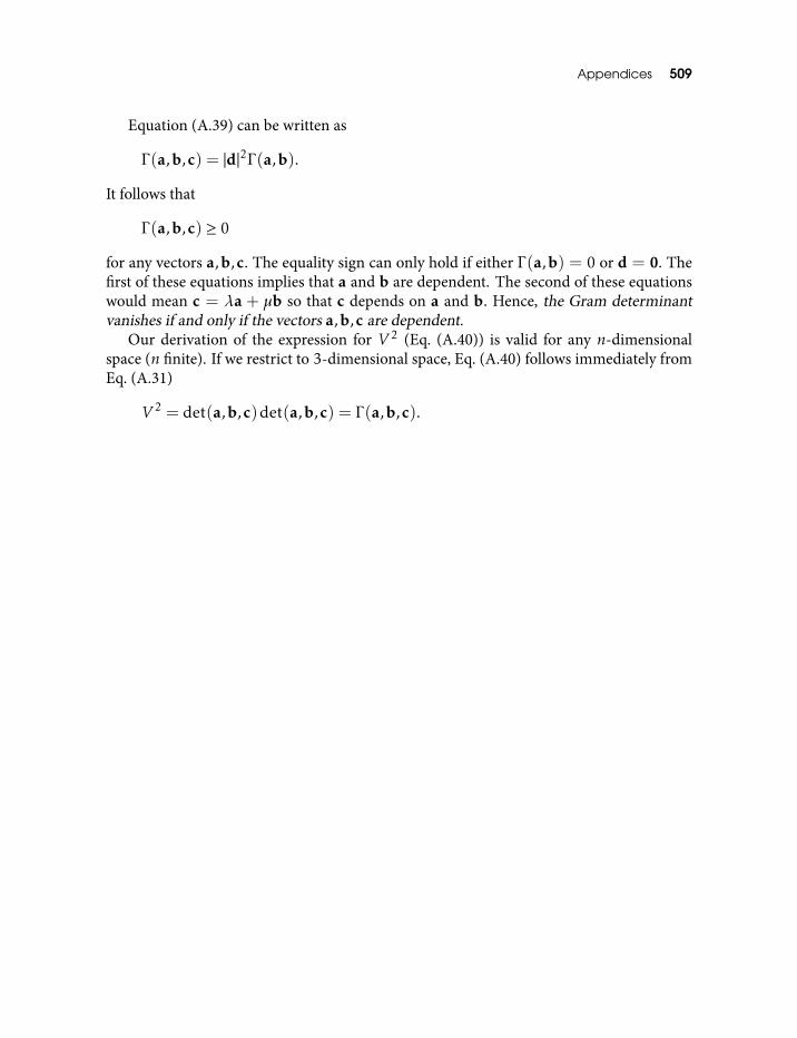
Appendices 509
Equation (A.39) can be written as
Γ (a,b,c) = |d|2Γ (a,b).
It follows that
Γ (a,b,c) ≥ 0
for any vectors a,b,c. The equality sign can only hold if either Γ (a,b) = 0 or d = 0. Thefirst of these equations implies that a and b are dependent. The second of these equationswould mean c = λa + µb so that c depends on a and b. Hence, the Gram determinantvanishes if and only if the vectors a,b,c are dependent.
Our derivation of the expression for V 2 (Eq. (A.40)) is valid for any n-dimensionalspace (n finite). If we restrict to 3-dimensional space, Eq. (A.40) follows immediately fromEq. (A.31)
V 2 = det(a,b,c)det(a,b,c) = Γ (a,b,c).
B
Dirac Delta Function
Consider the vector valued function
f(r) =rr2
which blows up at the origin. We know that this function is proportional to theelectrostatic field produced by a point charge at the origin. It is easy to see that at anyr , 0, the divergence of f, ∇ · f, is zero:
∇ · f = 1r2∂∂r
(r2 1r2
)=
1r2∂∂r
(1) = 0.
However, at r = 0 1r2 blows up and
(r2 1r2
)becomes indeterminate. Further, the surface
integral of f(r) over a sphere of radius R, centered at the origin, is∫f(r) · ds =
∫ ( rR2
)· (R2 sinθdθdφr)
=
(∫ π
0sinθdθ
)(∫ 2π
0dφ
)= 4π.
Thus, the surface integral remains finite despite the singularity at the origin. Now, werequire on physical grounds that the electrostatic field due to a point charge must obey thedivergence theorem. Hence, we must have∫
∇ · fdV = 4π
for any volume containing the origin. Since ∇ · f = 0 everywhere except at r = 0, all thecontribution to this integral must come from ∇ · f at the origin. Thus, ∇ · f has the bizarreproperty that it vanishes everywhere except at one point, the origin, and yet its integral over
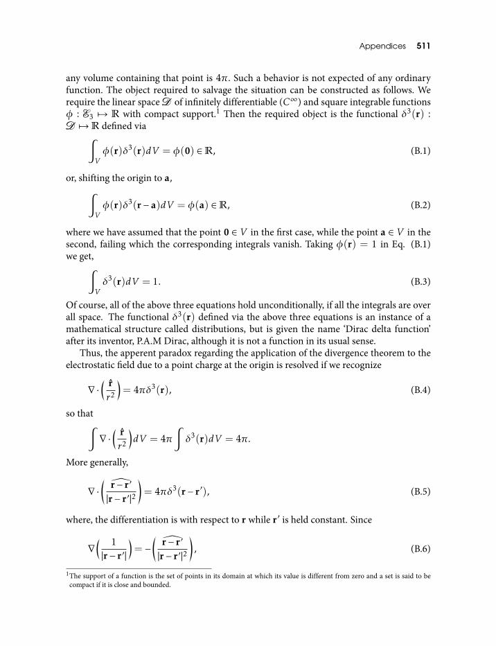
Appendices 511
any volume containing that point is 4π. Such a behavior is not expected of any ordinaryfunction. The object required to salvage the situation can be constructed as follows. Werequire the linear spaceD of infinitely differentiable (C∞) and square integrable functionsφ : E3 7→ R with compact support.1 Then the required object is the functional δ3(r) :D 7→R defined via∫
Vφ(r)δ3(r)dV = φ(0) ∈R, (B.1)
or, shifting the origin to a,∫Vφ(r)δ3(r− a)dV = φ(a) ∈R, (B.2)
where we have assumed that the point 0 ∈ V in the first case, while the point a ∈ V in thesecond, failing which the corresponding integrals vanish. Taking φ(r) = 1 in Eq. (B.1)we get,∫
Vδ3(r)dV = 1. (B.3)
Of course, all of the above three equations hold unconditionally, if all the integrals are overall space. The functional δ3(r) defined via the above three equations is an instance of amathematical structure called distributions, but is given the name ‘Dirac delta function’after its inventor, P.A.M Dirac, although it is not a function in its usual sense.
Thus, the apperent paradox regarding the application of the divergence theorem to theelectrostatic field due to a point charge at the origin is resolved if we recognize
∇ ·( rr2
)= 4πδ3(r), (B.4)
so that∫∇ ·
( rr2
)dV = 4π
∫δ3(r)dV = 4π.
More generally,
∇ ·(
r− r′
|r− r′ |2
)= 4πδ3(r− r′), (B.5)
where, the differentiation is with respect to r while r′ is held constant. Since
∇( 1|r− r′ |
)= −
(r− r′
|r− r′ |2
), (B.6)
1The support of a function is the set of points in its domain at which its value is different from zero and a set is said to becompact if it is close and bounded.
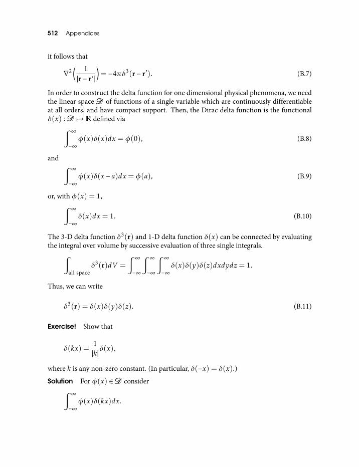
512 Appendices
it follows that
∇2( 1|r− r′ |
)= −4πδ3(r− r′). (B.7)
In order to construct the delta function for one dimensional physical phenomena, we needthe linear space D of functions of a single variable which are continuously differentiableat all orders, and have compact support. Then, the Dirac delta function is the functionalδ(x) :D 7→R defined via∫ ∞
−∞φ(x)δ(x)dx = φ(0), (B.8)
and ∫ ∞−∞φ(x)δ(x − a)dx = φ(a), (B.9)
or, with φ(x) = 1,∫ ∞−∞δ(x)dx = 1. (B.10)
The 3-D delta function δ3(r) and 1-D delta function δ(x) can be connected by evaluatingthe integral over volume by successive evaluation of three single integrals.∫
all spaceδ3(r)dV =
∫ ∞−∞
∫ ∞−∞
∫ ∞−∞δ(x)δ(y)δ(z)dxdydz = 1.
Thus, we can write
δ3(r) = δ(x)δ(y)δ(z). (B.11)
Exercise! Show that
δ(kx) =1|k|δ(x),
where k is any non-zero constant. (In particular, δ(−x) = δ(x).)
Solution For φ(x) ∈D consider∫ ∞−∞φ(x)δ(kx)dx.
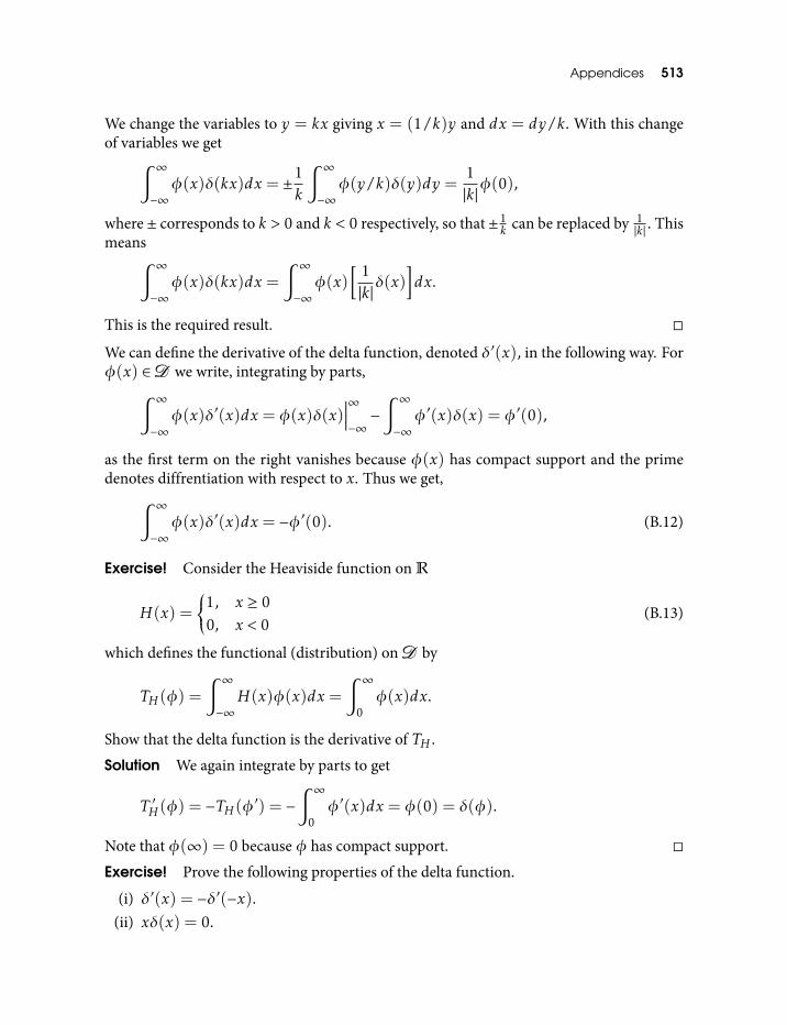
Appendices 513
We change the variables to y = kx giving x = (1/k)y and dx = dy/k. With this changeof variables we get∫ ∞
−∞φ(x)δ(kx)dx = ±1
k
∫ ∞−∞φ(y/k)δ(y)dy =
1|k|φ(0),
where ± corresponds to k > 0 and k < 0 respectively, so that ±1k can be replaced by 1
|k| . Thismeans∫ ∞
−∞φ(x)δ(kx)dx =
∫ ∞−∞φ(x)
[ 1|k|δ(x)
]dx.
This is the required result.
We can define the derivative of the delta function, denoted δ′(x), in the following way. Forφ(x) ∈D we write, integrating by parts,∫ ∞
−∞φ(x)δ′(x)dx = φ(x)δ(x)
∣∣∣∣∞−∞−∫ ∞−∞φ′(x)δ(x) = φ′(0),
as the first term on the right vanishes because φ(x) has compact support and the primedenotes diffrentiation with respect to x. Thus we get,∫ ∞
−∞φ(x)δ′(x)dx = −φ′(0). (B.12)
Exercise! Consider the Heaviside function on R
H(x) =
1, x ≥ 00, x < 0
(B.13)
which defines the functional (distribution) onD by
TH (φ) =
∫ ∞−∞H(x)φ(x)dx =
∫ ∞0φ(x)dx.
Show that the delta function is the derivative of TH .
Solution We again integrate by parts to get
T ′H (φ) = −TH (φ′) = −
∫ ∞0φ′(x)dx = φ(0) = δ(φ).
Note that φ(∞) = 0 because φ has compact support.
Exercise! Prove the following properties of the delta function.
(i) δ′(x) = −δ′(−x).(ii) xδ(x) = 0.
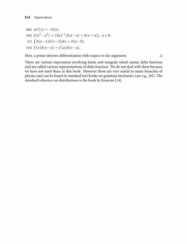
514 Appendices
(iii) xδ′(x) = −δ(x).(iv) δ(x2 − a2) = (2a)−1[δ(x − a) + δ(x+ a)], a > 0.
(v)∫δ(a− x)δ(x − b)dx = δ(a− b).
(vi) f (x)δ(x − a) = f (a)δ(x − a).
Here, a prime denotes differentiation with respect to the argument.
There are various expressions involving limits and integrals which mimic delta functionand are called various representations of delta function. We do not deal with them becausewe have not used them in this book. However these are very useful in many branches ofphysics and can be found in standard text books on quantum mechanics (see e.g., [6]). Thestandard reference on distributions is the book by Kesavan [14].
Bibliography
1. Ahlfors, L. V. 1979. Complex Analysis. New York: Tata McGraw-Hill.2. Antia, H. M. 1991. Numerical Methods for Scientists and Engineers. New Delhi: Tata
McGraw-Hill Publishing Company.3. Arnold, V. I. 1989. Mathematical Methods of Classical Mechanics. New York:
Sprienger-Verlag.4. Ashcroft, N. W., and Mermin, N. D. 1976. Solid State Physics. Fort Worth: Harcourt
Brace College Publishers.5. Courant, R., and John, F. 1974. Introduction to Calculus and Analysis. Vol. I & II.
New York: John Wiley and Sons.6. Cohen-Tannoudji, C., Diu, B., and Laloe, F. 1991. Quantum Mechanics. Vol. I & II.
Wiley-VCH.7. Doran, C. J. L., and Lasenby, A. N. 2003. Geometric Algebra for Physicists.
Cambridge: Cambridge University Press.8. Fleisch D. 2011. A Student’s Guide to Vectors and Tensors. Cambridge: Cambridge
University Press.9. Griffiths, D. J. 1999. Introduction to Electrodynamics. New Delhi: Prentice-Hall of
India Pvt. Ltd.10. Hestenes, D. 1986. New Foundations for Classical Mechanics. Dordrecht: Kluwer
Academic Publishers.11. Hestenes, D., Sobczyk, G. 1987. Clifford Algebra to Geometric Calculus: A Unified
Language for Mathematics and Physics. (Fundamental Theories of Physics).Dordrecht: Springer.
12. Horn, R. A., and Johnson, C. R. 1985. Matrix Analysis. Vol. I & II. Cambridge:Cambridge University Press.
13. Jackson, J. D. 1999. Classical Electrodynamics. New York: John Wiley and Sons.14. Kesavan, S. 1989. Topics in Functional Analysis and Applications. New Delhi: Wiley.
516 Bibliography
15. Lang, S. 1973. Calculus of Several Variables. Reading, Massachusetts:Addison-Wesley.
16. Munk, W. H., and Macdonald, G. J. F. 1960. The Rotation of the Earth. Cambridge:Cambridge University Press.
17. Rajaraman, V. 2009. Computer Oriented Numerical Methods. New Delhi: Prentice-Hall of India.
18. Raju, C. K. 2007. Cultural Foundations of Mathematics: The Nature of MathematicalProof and the Transmission of Calculus from India to Europe in the 16th c. CE. Delhi:Pearson Longman
19. Rana, N. C., and Joag, P. S. 1991. Classical Mechanics. New Delhi: Tata McGraw-HillPublishing Company Limited.
20. Rosenberg, C.B. Private communication.21. Schey, H. M. 2005. Div, Grad, Curl, and all that: an informal text on Vector Calculus.
4th Ed. New York: W. W. Norton22. Schwartz, M., Green, S. and Rutledge, W. A. 1960. Vector Analysis with Applications
to Geometry and Physics. New York: Harper & Brothers.23. Shorter, L. R. 2014. Problems and Worked Solutions in Vector Analysis. Mineola,
New York: Dover Publications, Inc.24. Stacey, F. D. 1969. Physics of the Earth. New York: John Wiley & Sons Inc.25. Sudarshan, E. C. G., and N. Mukunda. 1974. Classical Dynamics: A Modern
Perspective. New York: Wiley.26. Zwikker, C. 1950. Advanced Plane Geometry. Amsterdam: North Holland Publishing
Company.
Index
Acceleration 17Active transformation 180Addition of vectors 8Adjoint of an operator 117Admittance of an electrical circuit 106Affine equivalent 206Affine group 206Affine transformations 206Analytic function 265Angle 4
Angle between vectors 12Angular momentum 38
Conservation of 468Arc length parameterization 225Axial vector 36
Baricentric coordinates 81see also (Homogeneous coordinates) 81
Basis 21Binormal 230Boundary point 217Boundary point of a set 217Brachistochrone 258Bravais lattice 43
Primitive cell of 43
C1-invertible 284Cardinality of a set 216Cardioid 255Cauchy–Riemann conditions 484Cauchy–Schwarz inequality 28, 33Center of mass 14Central conics 206Central quadrics 209
Centripetal acceleration 233Chain rule 263, 274Change of basis 132Chasles theorem 204Circle of Apollonius 102Circle of curvature 228Circle transformation 108Circular orbit 468Closed set 217Colinear 15Collineations 206Commuting operators 116Components of a vector 21Composition of rotations 179Composition of symmetry elements 183Conformal transformations 101Congruence 205Conic sections 90Conicoid 91Conics 206Continuous functions 220Continuous groups 197Convergence of a sequence 217Convergent sequence 218Coordinate axes 18Coordinate functions 225Coordinate line 57Coordinate lines 18Coordinate planes 18Coordinate surface 59Coordinate system 18
Dextral 19Left handed 19Right handed 19
Coordinates of a vector 21
518 Index
Coplanar 15Lines 6
Countable set 216Cramer’s rule 123Criterion for orthogonal vectors in a plane 98Criterion for parallel vectors in a plane 98Cross product
see also (Vector product) 32Cross ratio 100Curl in spherical polar coordinates
in cylindrical coordinates 321Curl of a vector field 306Curvature 227Cycloid 253Cyclotron frequency 477
Darboux vector 233Decomposition of vectors
see also (Resolution of vectors) 13Determinant of an operator 119Dextral coordinate system
see also (Right handed coordinate system) 18Diagonalizable operator 134Diameter of a set 217Differential of a function 280Dimension 4, 20Direct lattice 44Directance 75Direction 4Direction cosines 24Directional derivative 266Directions of tangent and normal 261Directrix 91Distance between vectors 28Distributive property
Multiplication by scalars 10Divergence in spherical polar coordinates
in cylindrical coordinates 321divergence of a vector field 304Division ratio 80Domain 215Domain of an operator 116Dot product 22Drift velocity 482
Eccentric anomaly 248Eccentricity 91Eigenvalue 134Eigenvector 134Ellipsoid 147
Entire function 265Epicycloid 254Epitrochoids 258Equipotential surface 283Equivalence relation 205, 206Euclidean group 199, 201Euclidean metric 30Euler angles 184Euler’s theorem 188Evolutes and involutes 243Extended associative law 192Extended inverse 192
Faithful representation 196Finite set 216Focus 91Force 17Frenet-Seret formulae 232
Gaussian fundamental quantities 301General (complex) equation to a circle 105Geodesic 30Geometric calculus 273Gradient in spherical polar coordinates
in cylindrical coordinates 321Gradient of a potential 282Gram determinant 42, 407Group (definition) 191Group of isometries 199
Harmonic oscillator 450Hodograph 456Homogeneous coordinates
see also (Baricentric coordinates) 81Homomorphism 45Hyperboloid of one sheet 147Hyperboloid of two sheets 147Hypocycloid 256Hypotrochoids 258
Identity operator 117Image set 117, 215Impedance of an electrical circuit 106Implicit function theorem 285Implicit functions 283, 285Infinite set 216Infinitesimal rotations 171Inner product 22Interior point 217Interior point of a set 217
Index 519
Intrinsic equation of a space curve 240Inverse
Multiplicative 23Inverse mapping theorem 284Inverse maps 283Inverse of a matrix 495Inverse of a vector
Additive 9Inverse operator 118Inversion 103Invertible operator 118Isomorphism 45
Jacobian determinant 277, 285, 287, 293Jacobian matrix 277, 279, 285Jerk 233
Kepler’s equation 253Kepler’s third law 468Kronecker delta 24
Laplacian in spherical polar coordinatesin cylindrical coordinates 321
Law of cosines 11, 26Law of sines 12, 35left handed coordinate system 18Levi-Civita symbols 44, 48Limit of a converging sequence 218Line element 302Line element on the torus 304Linear combination of vectors 11Linear form 497Linear momentum 38Linear operator 115Linear space 47Linear transformation 115Linearly dependent vectors 20Linearly independent vectors 20Lissajous figure 455Lissajous motion 249
Matrices 129Matrices representing rotations 176Matrix representing an operator 129Method of successive approximations 253Method of successive approximations 289Metric space 47Mobius rules 100Mohr’s algorithm
Graphical implementation 150
Mohr’s algorithm 147Mohr’s circle 150Moment of a line 76Moment of force 38Moving trihedral 231
Natural equation of a space curve 240Negatively oriented triplet 68Non-coplanar
Vectors 15Non-coplanar lines 6Non-singular operators 121Norm of a vector 22Normal plane 236
One to one correspondence 118One to one map or function 118, 215Onto map or function 118, 215Open set 217Order of contact 238Orientation of a plane 72Orientation relative to a coordinate system 69Oriented volume 40Orthogonal operator 158Orthogonal transformations 158Orthogonal vectors 12Orthonormal basis 21Osculating circle 228, 239Osculating plane 236
Parabolic coordinates 61Parameterization of a curve 225Parametric representation of a sphere 298Partial derivative 267Passive transformation 181Plane
Equation in normal form 85Plane wave 85Planes 83Point function 67point of division 80Polar coordinates 26Polar Decomposition Theorem 166Polar vector 36Position vectors 7Positive and negative sides of a curve 260Positively oriented triplet 68Potential of a vector field 282Principal axes 135Principal axes system 135
520 Index
Principal normal 227principal values 167principal vectors 167Product of two linear operators 116Product rule 274Projectile motion 456Pseudo-scalar 40Pseudo-vector 36
Quadratic differential form 302
r-neighborhood of a point 217Radian measure 4Radians 89Radius of a set 217Radius of curvature 227Range 215Range of an operator 116Reciprocal frames 124Reciprocal lattice 44Reciprocal lattice of a crystal 43Rectifying plane 236Reflection
Orthogonal operator for 161Reflection operator
Canonical form of 161Regular point 225Representation of a group 196Resolution of vectors
see also (Decomposition of vectors) 13Right handed coordinate system
see also (Dextral coordinate system) 18Rigid body 38Rotation
as an orthogonal transformation 158Counterclockwise 5
Rotation group 196
Scalar 3Scalar integration 263Scalar product 22
Distributive property 25Scalar product as potential energy 30Scalar triple product 39
Sequence 217Shear 168Sign of curvature 262Similar figures 205Similarities 206Similarity transformation 205Similarity transformations 133Skewsymmetric operator 126Space 4Spectral decomposition 143Spectral form 143Spheres 89Spherical triangle 89Stereographic image 298Stereographic projection 298Straight lines 74Stram line 484Surfaces, parametric representation of 297Symmetric matrix 155Symmetric operator 126, 141Symmetry 181Symmetry breaking 183Symmetry element 181
Tautochrone 258Taylor series 264, 278Tensor 49, 115Tesserals 245Topocentric frame 462Torous, parametric representation of 303Torque 38Torsion 231Trochoids 258True anomaly 248
Uncountable set 216
Variation on a curve 281Vector fields 67Vector identities 52Vector product
see also (Cross product) 32Vector triple product 45Velocity space 456