An Inventory-Location Model: Formulation, Solution ... · Formulation, Solution Algorithm and Computational ... We argue that the importance of inventory management ... inventory

Daskin, Coullard and Shen 1 03/18/01

An Inventory-Location Model: Formulation, Solution Algorithm and

Computational Results

Mark S. Daskin Collette R. Coullard

Department of Industrial Engineering and Management Sciences Northwestern University

Evanston, IL 60208

Z. J. Max Shen Department of Industrial Engineering

303 Weil Hall P.O. Box 116595

University of Florida Gainesville, FL 32611-6595

February, 2001 Acknowledgements: This work was supported by NSF grants DMI-9634750 and DMI-9812915. This support is gratefully acknowledged.


ABSTRACT

We introduce a new distribution center (DC) location model that incorporates working inventory and safety stock inventory costs at the distribution centers. In addition, the model incorporates transport costs from the suppliers to the DCs that explicitly reflect economies of scale through the use of a fixed cost term. The model is formulated as a non-linear integer-programming problem. Model properties are outlined. A Lagrangian relaxation solution algorithm is proposed. By exploiting the structure of the problem we can find a low-order polynomial algorithm for the non-linear integer programming problem that must be solved in solving the Lagrangian relaxation subproblems. A number of heuristics are outlined for finding good feasible solutions. In addition, we describe two variable forcing rules that prove to be very effective at forcing candidate sites into and out of the solution. The algorithms are tested on problems with 88 and 150 retailers. Computation times are consistently below one minute and compare favorably with those of an earlier proposed set partitioning approach for this model (Shen, 2000; Shen, Coullard and Daskin, 2000). Finally, we discuss the sensitivity of the results to changes in key parameters including the fixed cost of placing orders. Significant reductions in these costs might be expected from e-commerce technologies. The model suggests that as these costs decrease it is optimal to locate additional facilities.


1. Introduction

Managing inventory has become a major challenge for firms as they

simultaneously try to reduce costs and improve customer service in today’s increasingly

competitive business environment. Managing inventory consist of two critical tasks.

First, we must determine the number of stocking locations or distribution centers to have.

Second, we must determine the amount of inventory to maintain at each of the centers.

Often these tasks are undertaken separately, resulting in a degree of suboptimization. In

this paper, we outline an integrated approach to determining the number of distribution

centers to establish and the magnitude of inventory to maintain at each center.

We argue that the importance of inventory management as outlined above has, if

anything, been heightened by e-commerce. Whether it is business to consumer (B2C) or

business to business (B2B), e-commerce end customers expect high levels of service and

speedy deliveries. At the same time, many of the inputs to traditional inventory

management decision-making are changing rapidly. E-commerce offers the hope of

significantly reducing order costs thereby allowing smaller more frequent shipments.

The model we propose below explicitly includes order shipment costs. As a result it is

capable of estimating the impacts of sharply reduced ordering costs on the number of

distributions centers, their locations, and the optimal inventory ordering policy. E-

commerce can also reduce variability across the supply chain by making end customer

orders visible throughout the chain. This visibility should reduce the bullwhip effect

(Lee, Padmanabhan and Whang, 1997; Lee, 1996; Simchi-Levi, Kaminsky and Simchi-

Levi, 2000). Our model does not directly account for these effects of e-commerce though

the model does explicitly consider safety stock inventories at the distribution centers

which are a function of the variability of customer demand.

This work was motivated by a study at a local blood bank conducted by two of the

authors. The blood bank supplied roughly 30 hospitals in the greater Chicago area. Our

focus was on the production and distribution of platelets, the most expensive and most

perishable of all blood products. If a unit of platelets is not used within 5 days of the time

it is produced from whole blood, it must be destroyed. The demand for platelets is highly

variable as they are needed in only a limited number of medical contexts. When they are


used, however, multiple units are often needed. The hospitals supplied by the blood bank

collectively owned the blood bank and set prices. As a result they could return a unit of

platelets up to the time it outdated and not be charged for it. Thus, there was little

incentive to manage inventories in an efficient manner. Many of the larger hospitals

ordered almost twice the number of platelet units that they used each year resulting in the

need to destroy thousands of units of this expensive blood product. Other hospitals

ordered almost all of their needed platelets on a STAT or emergency basis. The blood

bank often had to ship the units to these hospitals using a taxi or express courier at

significant expense to the system. Clearly an improved system was needed. We

proposed a revision to their pricing policies along with a system in which selected

hospitals would maintain an inventory of platelets for use in neighboring hospitals. This

would allow the system to take advantage of the risk-pooling effect. We selected the

hospitals at which inventory would be maintained using a P-median model (Hakimi,

1963, 1964; Daskin, 1995). The model did not account directly for the working

inventory or safety stock (risk-pooling) effects, for the transport costs from the blood

bank to the selected hospitals or the fixed costs of establishing the facilities. Clearly, this

was only a first-cut approach. The research outlined below is aimed, in part, at

developing a more comprehensive and more accurate model of such a situation.

The remainder of this paper is organized as follows. In section 2 we review

relevant related literature. The model we propose is formulated in section 3. The

formulation we obtain is a mixed integer non-linear programming problem which can be

viewed as an extension of the traditional uncapacitated fixed charge facility location

problem. In addition to the standard facility location and local distribution costs, the

model includes cost components representing working and safety stock inventories at the

distribution centers as well as transport costs from the supplier(s) to the distribution

centers. These inventory and supplier-to-DC transport costs introduce significant non-

linearities into the model. Section 4 outlines a number of key properties of the model we

propose and introduces an additional assumption on the demand distributions that we use

to develop a solution algorithm for the problem. Section 5 outlines our solution

procedure for the problem. Computational results are presented in section 6. In section

7, we present our conclusions and outline directions for future work.


2. Literature Review

Inventory theory literature tends to focus on finding optimal inventory

replenishment strategies at the DCs and the retailer outlets. This work usually assumes

that the number and locations of the DCs are given. See, for example, Graves et al.

(1993), Nahmias (1997) and Zipkin (1997). On the other hand, location theory tends to

focus on developing models for determining the number of DCs and their locations, as

well as the DC-retailer assignments. This work usually includes fixed facility setup costs

and transportation costs, but the operational inventory and shortage costs are typically

ignored. Daskin and Owen (1999) provide an overview of facility location modeling as

do the recent texts by Daskin (1995) and Drezner (1995).

Eppen (1979) studied the so-called “risk pooling effects,” namely the effects of

inventory-cost savings achieved by grouping retailers. Assume customer demands are

normally distributed with a mean iµ and a standard deviation iσ for customer i. Then the

expected total inventory cost under the decentralized mode for n retailers is ∑=

n

iiK

1σ . If

the demands of the n retailers are independent, the optimal cost under a centralized mode

can be expressed by ∑=

n

iiK

1

2σ , which is less than ∑=

n

iiK

1σ , where K is a constant

depending on the holding and penalty costs and the standard normal loss function.

Recently, there are several new studies that combine inventory management and

routing decisions. For example, Federgruen and Zipkin (1984), Federgruen and Simchi-

Levi (1995), Viswanathan and Mathur (1997), Chan, Federgruen, and Simchi-Levi(1998)

and Kleywegt, Nori, and Savelsbergh (2000).

Also, several models combine location and routing decisions; for instance,

Laporte and Dejax (1989), Berman, Jaillet and Simchi-Levi (1995), and Berger, Coullard

and Daskin (1998).

Shen, Coullard and Daskin (2000) studied model presented below, but they use

set partitioning approach. We compared our computational results with theirs. Teo, Ou


and Goh (2000) studied the impact on inventory costs with consolidation of distribution

centers. They also propose an algorithm that solves for a distribution system with the

total fixed facility location cost and inventory costs within 2 of the optimal. But they

ignore the costs to ship from the supplier to the DCs and from the DCs to the retailers in

their model. Finally, Erlebacher and Meller (2000) formulate a highly non-linear integer

location/inventory model. They attack the problem by using a continuous approximation

as well as a number of construction and bounding heuristics. For problems with 16

customers, they obtained solutions that were between 3.78% and nearly 36% of a lower

bound. An exchange heuristic improved the solution considerably. Computation times

on a 600 node problem using the exchange heuristic averaged 117 hours on a Sun Ultra

Sparcstation.

3. Model Formulation

We consider a three-tiered system consisting of one or more suppliers,

distribution centers and retailers. We assume that the locations of the suppliers and the

retailers are known and that the suppliers have infinite capacity at least from the

perspective of the system being modeled. The problem is to determine the optimal

number of distribution center, their location, the retailers assigned to each distribution

center, and the optimal ordering policy at the distribution centers. We do not explicitly

model the inventory maintained by the retailers themselves. A key problem is that the

demand that is seen by each distribution center is a function of the demands at the

retailers assigned to the distribution center. Thus, the inventory policy – the reorder

interval, reorder size, and safety stock – at the distribution center is a function of the

assignment of retailers to the distribution center. Since these assignments are not known

a priori, the inventory policy must also be endogenously determined.

To begin modeling the problem, let us assume for the moment that we know

which customers are to be assigned to a specific distribution. center. Assume that the

demand at each retailer is Normally distributed with a daily mean of µi and a daily

variance of σ2i and let S be the set of customers assigned to the distribution center. Let

L be the lead time in days for deliveries from the supplier to the distribution center.


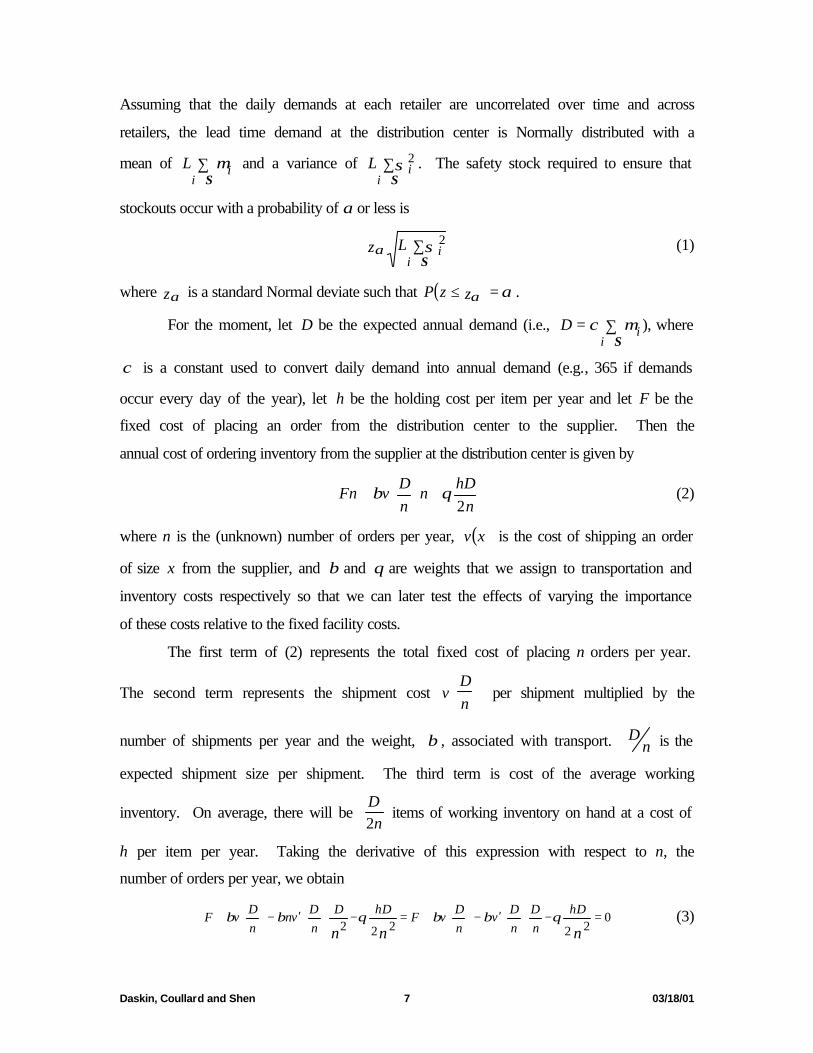
Assuming that the daily demands at each retailer are uncorrelated over time and across

retailers, the lead time demand at the distribution center is Normally distributed with a

mean of ∑∈Si

iL µ and a variance of ∑∈Si

iL σ2 . The safety stock required to ensure that

stockouts occur with a probability of α or less is

∑∈Si

iLz σα2 (1)

where zα is a standard Normal deviate such that ( ) αα =≤ zzP .

For the moment, let D be the expected annual demand (i.e., ∑=∈ Si

iD µχ ), where

χ is a constant used to convert daily demand into annual demand (e.g., 365 if demands

occur every day of the year), let h be the holding cost per item per year and let F be the

fixed cost of placing an order from the distribution center to the supplier. Then the

annual cost of ordering inventory from the supplier at the distribution center is given by

n

hDn

nD

vFn2

θβ +

+ (2)

where n is the (unknown) number of orders per year, ( )xv is the cost of shipping an order

of size x from the supplier, and β and θ are weights that we assign to transportation and

inventory costs respectively so that we can later test the effects of varying the importance

of these costs relative to the fixed facility costs.

The first term of (2) represents the total fixed cost of placing n orders per year.

The second term represents the shipment cost vDn

per shipment multiplied by the

number of shipments per year and the weight, β , associated with transport. Dn is the

expected shipment size per shipment. The third term is cost of the average working

inventory. On average, there will be Dn2

items of working inventory on hand at a cost of

h per item per year. Taking the derivative of this expression with respect to n, the

number of orders per year, we obtain

022222

=−

′−

+=−

′−

+

nnn

hDnD

nD

vnD

vFhDD

nD

vnnD

vF θββθββ (3)


If ( )v x is linear in x (e.g., if ( )v x g ax= + ) then ( )′v x is a constant (e.g., a) and the

expression above becomes

02222

=−+=−−++nn

hDgF

hDnD

anD

agF θβθβββ (4)

Solving for n, we obtain ( )gFhD

nβ

θ+

=2

. Substituting this into the cost function (2) we

obtain a working inventory cost of

( ) ( )( )

( ) ( ) ( ) aDgFhDgFhD

aDgFhD

hDgFhD

aDgF

hDg

gFhD

F

ββθβθ

ββθ

θβ

θββ

θβ

βθ

++=+

+++

=+

+++

++

222

2222 (5)

Recall that this cost includes the costs of placing orders at the distribution center,

transporting goods from the supplier to the distribution center and holding the working

inventory at the DC.

Unfortunately, the derivation of the safety stock (1) and the working inventory

cost (5) assume that we know the assignment of retailers to the distribution center as

denoted by the set S. The identity of this set is not known a priori and must be

determined endogenously.

To simultaneously determine the locations of the DCs, assignments of the retailers

to the DCs, and working and safety stock inventory costs, let us define the following

additional inputs and sets:

I set of retailers indexed by i J set of candidate DC sites indexed by j f j fixed (annual) cost of locating a distribution center at candidate site j, for

each J∈j

d ij cost per unit to ship between retailer i and candidate DC site j, for each

I∈i and J∈j χ days per year (used to convert daily demand and variance values to annual

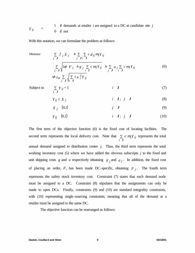
values). In addition, we define the following decision variables:

=not if0

site candidateat locate weif1 jX j


=not if0

site candidateat DC a toassigned are retailer at demands if1 jiY ij

With this notation, we can formulate the problem as follows:

∑ ∑

∑ ∑∑ ∑

∑ ∑∑

∈ ∈

+

∈ ∈+

∈ ∈

+

+

∈ ∈+

∈

J I

J IJ I

J IJ

j iijiLh

j iijij

j iijijjh

j iijiij

jjj

Yz

YaYgF

YdXf

σ

µµ

µ

αθ

χβχβθ

χβ

2

2

Minimize

(6)

1Subject to =∑∈Jj

ijY I∈∀i (7)

XY jij ≤ I∈∀i ; J∈∀j (8)

{ }1,0∈X j J∈∀j (9)

{ }1,0∈Y ij I∈∀i ; J∈∀j (10)

The first term of the objective function (6) is the fixed cost of locating facilities. The

second term represents the local delivery cost. Note that ∑∈Ii

ijiYµχ represents the total

annual demand assigned to distribution center j. Thus, the third term represents the total

working inventory cost (5) where we have added the obvious subscripts j to the fixed and

unit shipping costs g and a respectively obtaining g j and a j . In addition, the fixed cost

of placing an order, F, has been made DC-specific, obtaining F j . The fourth term

represents the safety stock inventory cost. Constraint (7) states that each demand node

must be assigned to a DC. Constraint (8) stipulates that the assignments can only be

made to open DCs. Finally, constraints (9) and (10) are standard integrality constraints,

with (10) representing single-sourcing constraints, meaning that all of the demand at a

retailer must be assigned to the same DC.

The objective function can be rearranged as follows:


( )

∑ ∑∑∑

∑ ∑∑ ∑

∑ ∑∑

∈

∈Θ+

∈+

∈+

=∈ ∈

+

∈ ∈

+

+

∈ ∈++

∈

J III

J IJ I

J IJ

j iiji

iijij

iijijjj

j iijiLh

j iijijjh

j iijjiji

jjj

YYKYdXf

YzYgF

YadXf

σµ

σµ

µ

αθχβθ

χβ

ˆˆ 2

22

Minimize

(11)

where

( )

σσ

µ

αθ

βχθ

βχ

22

2

ˆ

ˆ

iLi

hjjhj

jijiij

z

gFK

add

=

=Θ

+=

+=

In (11) we have grouped the linear term representing the marginal transport costs from

the supplier to the distribution center (represented by terms in a j ) with the local delivery

costs (represented by terms in d ij ). Thus, d ijˆ captures local delivery costs from the

DCs to the retailers as well as the marginal cost of shipping a unit from a supplier to a

DC. K j captures the working inventory effects due to the fixed ordering costs at the DC

as well as the fixed transport costs from a supplier to a DC. Finally, Θ captures the

safety stock costs at the distribution centers.

The constraints (7)-(10) are identical to those of the traditional uncapacitated

fixed charge facility location problem (Balinski, 1965; Erlenkotter, 1978; Korkel, 1989).

Thus, the solution approach that we propose below mirrors some of the solution

approaches used for that problem. However, these approaches must be modified

significantly to account for the final two non-linear terms in the objective function (11).

4. Model properties

Before outlining the solution approach, it is worth noting a number of properties

of the model. First, unlike the traditional uncapacitated fixed charge location model in

which it is always optimal to assign demands to the facility that can serve the demands at


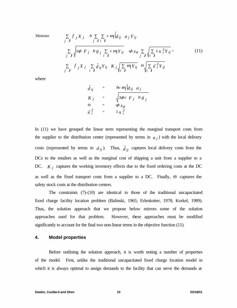
least cost (i.e., the facility j with the smallest value of d ij for retailer i), in this problem it

may be optimal to assign retailers to a more remote distribution center. Doing so may

reduce the working inventory, safety stock inventory and transport costs from the

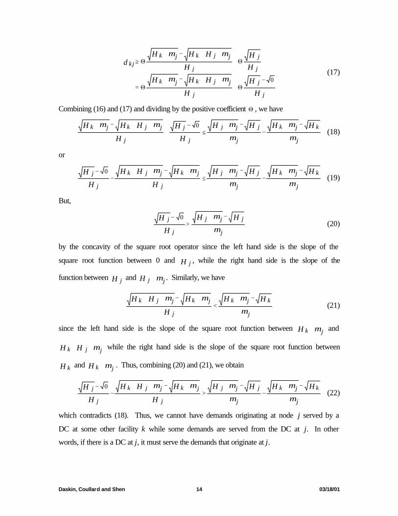
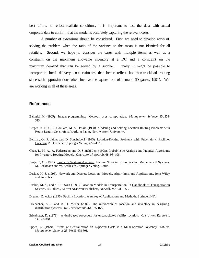
supplier to the DC sufficiently to offset the increased local delivery costs. Figure 1

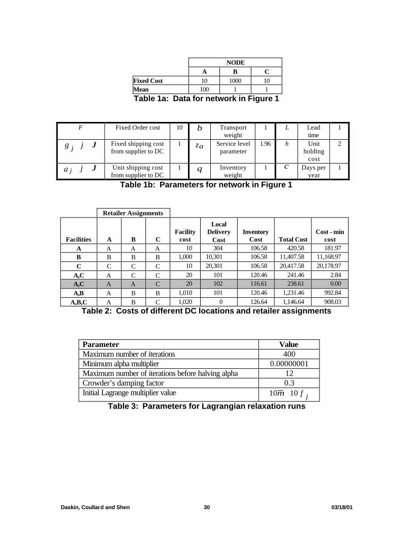
illustrates a small example in which this occurs. Table 1 provides the input data and

parameters for the problem while Table 2 compares the total costs for different DC

locations and different customer assignments for the problem. The first column gives the

DC locations; the next three give the retailer assignments to DCs; the next three give the

facility, local delivery and inventory cost terms; and the last two columns give the total

cost and the difference between the optimal total cost and the cost of the solution

indicated in that row. In this example, it is optimal to assign demands at retailer B to a

facility at A with a cost per unit shipped of 101 despite the fact that there is a facility at C

with a smaller unit shipping cost for the B to C channel.

Not only does this phenomenon occur in small (contrived) cases, but we have

found that it occurs in our computational results using realistic national demand data,

particularly when the inventory-related costs are large relative to the other costs (i.e.,

when θ is large relative to β ). Typically we find this behavior associated with small

retail nodes that almost equidistant to two different DCs. We also can construct

examples in which it is optimal to locate a DC at a particular node, but for demands from

that node to be assigned to a different DC. In other words, it is conceivable that the

optimal solution would locate a facility in Chicago, for example, but would assign

demands from Chicago to a facility in Minneapolis. Again, the intuitive reason for this is

that the reduction in inventory and supplier-to-DC transport costs (all of which entail

risk-pooling terms) more than offset the increased local delivery costs from the DC to the

retailers. The reader is referred to Shen (2000) or Shen, Coullard and Daskin (2000) for a

simple example in which this occurs. In practice, it is unlikely that a supply chain

manager would organize her distribution system in this way even if doing so would result

in small cost savings. Fortunately, we will be able to prove that this does not occur once

we make one additional assumption.


To simplify the model somewhat further we assume that the variance-to-mean

ratio at each retailer is identical for all retailers. In other words, we assume that γµσ =

i

i2

,

I∈∀i . While this may seem like a restrictive assumption, if demands arise from a

Poisson process, then this assumption is exact and we are merely approximating a

Poisson demand process by Normally distributed demands, which is a good

approximation for sufficiently large demand values (Montgomery, Runger and Hubele,

1998). Also, in many other contexts (e.g., transportation planning with random travel

times) it is common to assume a single variance-to-mean ratio (Sheffi, 1985). With this

assumption, the objective function can be rewritten as

∑ ∑∑

∑ ∑∑∑

∑ ∑∑∑

∈

∈+

∈+

=∈

∈Θ+

∈+

∈+

=∈

∈Θ+

∈+

∈+

J II

J III

J III

j iijij

iijijjj

j iijiL

iijij

iijijjj

j iiji

iijij

iijijjj

YKYdXf

YYKYdXf

YYKYdXf

µ

µµ

σµ

γ

ˆˆ

ˆ

ˆˆ 2Minimize

(12)

where γLKK jj Θ+=ˆ .

This assumption does two things. First, it reduces the number of non-linear terms

from two to one. This will facilitate the solution approach outlined below in section 5.

Second, as shown in the following theorem, under this assumption it is never optimal to

open a DC at a node and to then serve the demands from that node from another DC.

Theorem: If α>0.5, 0>θ and h>0 and all inter-nodal distances are positive and

I∈∀= iii 2 γµσ , then if there is a DC at node j then demands at node j are served by

that DC.

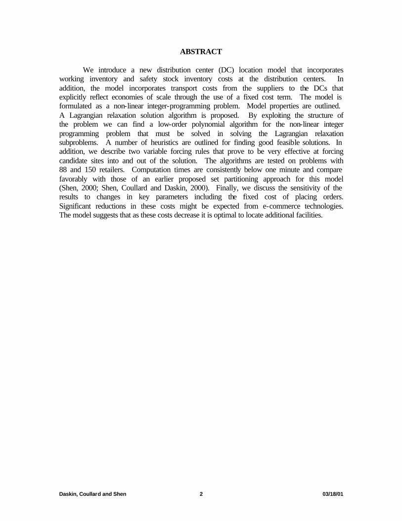
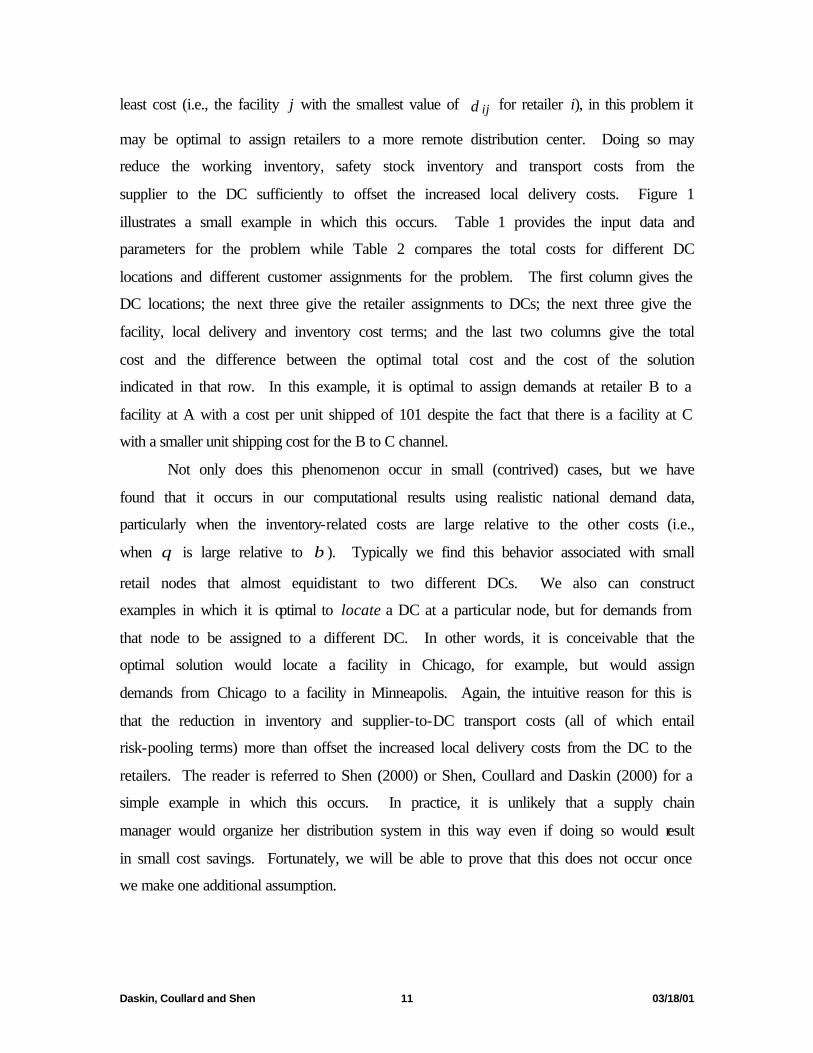
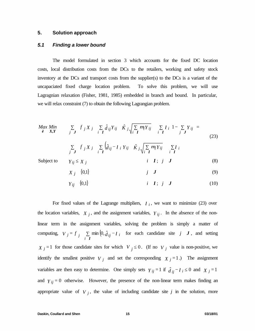
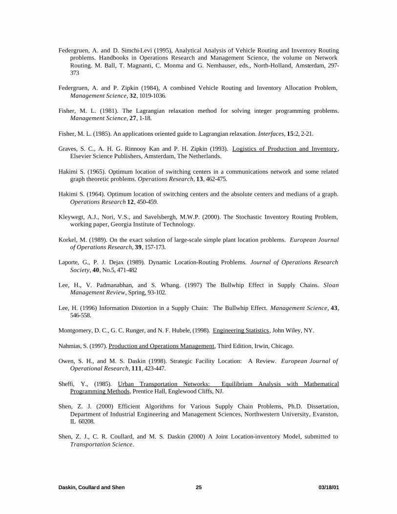
Proof: Assume that there is a DC at node j, but that the demands at node j are served by

a DC at some other node, node k in an optimal solution. Since there is a DC at node j,

there must be other demand nodes with a total positive mean demand that are assigned to

the DC at j. Let this total mean demand be H j . Similarly, let H k be the total mean


demand assigned to the DC at node k excluding the demand originating at node j whose

mean value is µ j . (Note that while H k is defined to include the demand originating at

node k, H j does not include the demand originating at node j.) Let d kj be the cost of

shipping one unit of demand from k to j and, as before, zh αθ=Θ . This situation is

illustrated in Figure 2 below.

Since serving the demand that originates at j from the facility at k is (assumed to

be) optimal, we have

HHHHd kjjjjkjk j Θ++Θ≤Θ++Θ+ µµµ (13)

or the cost of serving the demand originating at node j from k is less than or equal to the

cost of serving the demand originating at node j from the facility at j. Also, we have

µµµµ jjkjk jjk jjjkjk j HHHddHHd ++Θ++≤Θ++Θ+ ~ (14)

or the cost of serving the demand originating at node j from k and serving other demands

( H j ) at node j is less than the cost of serving the demand at node j from node k and

serving the demand assigned to node j from the facility at k. Doing the latter incurs an

additional transport cost per unit of dd kjkj ≤~ since the demands assigned to node j can

always be routed through j when served from k. Note that the term Hd jkj~ does not

represent the total local delivery cost for the demands that are being reassigned from j to

k; rather it represents the average additional cost of assigning these demands from j to k.

Thus, we can rewrite (14) as

( ) µµ

µµµµ

jjkjjk j

jjkjk jjk jjjkjk j

HHHd

HHHddHHd

++Θ++≤

++Θ++≤Θ++Θ+ ~

(15)

Rearranging (13) we have

µ

µ

µ

µ

j

kjk

j

jjjk j

HHHHd

−+Θ−

−+Θ≤ (16)

and rearranging (15) we have


H

H

H

HHH

H

H

H

HHHd

j

j

j

jjkjk

j

j

j

jjkjkkj

0−Θ+

++−+Θ=

Θ+++−+

Θ≥

µµ

µµ

(17)

Combining (16) and (17) and dividing by the positive coefficient Θ , we have

µ

µ

µ

µµµ

j

kjk

j

jjj

j

j

j

jjkjk HHHH

H

H

H

HHH −+−

−+≤

−+

++−+ 0 (18)

or

µ

µ

µ

µµµ

j

kjk

j

jjj

j

jkjjk

j

j HHHH

H

HHH

H

H −+−

−+≤

+−++−

− 0 (19)

But,

µ

µ

j

jjj

j

j HH

H

H −+>

− 0 (20)

by the concavity of the square root operator since the left hand side is the slope of the

square root function between 0 and H j , while the right hand side is the slope of the

function between H j and µ jjH + . Similarly, we have

µ

µµµ

j

kjk

j

jkjjk HH

H

HHH −+<

+−++ (21)

since the left hand side is the slope of the square root function between µ jkH + and

µ jjk HH ++ while the right hand side is the slope of the square root function between

H k and µ jkH + . Thus, combining (20) and (21), we obtain

µ

µ

µ

µµµ

j

kjk

j

jjj

j

jkjjk

j

j HHHH

H

HHH

H

H −+−

−+>

+−++−

− 0 (22)

which contradicts (18). Thus, we cannot have demands originating at node j served by a

DC at some other facility k while some demands are served from the DC at j. In other

words, if there is a DC at j, it must serve the demands that originate at j.


5. Solution approach

5.1 Finding a lower bound

The model formulated in section 3 which accounts for the fixed DC location

costs, local distribution costs from the DCs to the retailers, working and safety stock

inventory at the DCs and transport costs from the supplier(s) to the DCs is a variant of the

uncapaciated fixed charge location problem. To solve this problem, we will use

Lagragnian relaxation (Fisher, 1981, 1985) embedded in branch and bound. In particular,

we will relax constraint (7) to obtain the following Lagrangian problem.

( ) ∑∑ +

∑+∑ −+

=∑

∑−∑ +

∑+∑+

∈∈ ∈∈

∈ ∈∈ ∈∈

IJ II

I JJ IIYX,ë

ii

j iijij

iijiijjj

i jiji

j iijij

iijijjj

YKYdXf

YYKYdXfMinMax

λµλ

λµ

ˆˆ

1ˆˆ

(23)

XY jij ≤Subject to I∈∀i ; J∈∀j (8)

{ }1,0∈X j J∈∀j (9)

{ }1,0∈Y ij I∈∀i ; J∈∀j (10)

For fixed values of the Lagrange multipliers, λi , we want to minimize (23) over

the location variables, X j , and the assignment variables, Y ij . In the absence of the non-

linear term in the assignment variables, solving the problem is simply a matter of

computing, ( )∑ −+=∈Ii

iijjj dfV λˆ,0min for each candidate site J∈j , and setting

1=X j for those candidate sites for which 0≤V j . (If no V j value is non-positive, we

identify the smallest positive V j and set the corresponding 1=X j .) The assignment

variables are then easy to determine. One simply sets 1=Y ij if 0ˆ ≤− λiijd and 1=X j

and 0=Y ij otherwise. However, the presence of the non-linear term makes finding an

appropriate value of V j , the value of including candidate site j in the solution, more


difficult. To do so, we need to be able to solve a subproblem of the following form for

each candidate DC:

SP(j) ∑+∑=∈∈ II i

iii

iij ZcZbV~min (24)

{ }1,0subject to ∈Z i I∈∀i (25)

where λiiji db −= ˆ and 0ˆ 2 ≥= µiji Kc . In (24)-(25) we have replace the assignment

variables Y ij by Z i to simplify the notation since SP(j) is specific to DC j.

In Shen, Coullard and Daskin (2000), we show that this subproblem can be solved

by the following procedure.

Step 1: Partitioning the set I into three sets: { }0: ≥=+ bi iI , { }0 and 0:0 =<= cbi iiI

and { }0 and 0: ><=− cbi iiI . (We note that under our assumption of the

variance being proportional to the mean, the set I 0 will generally be empty.

We include it below for completeness.)

Step 2: Sort the elements of I − so that cb

cb

cb

n

n≤•••≤≤2

2

1

1 where I −=n .

Step 3: Compute the partial sums ∑+∑+∑+∑==

∈=

∈∈∈

−−

m

ii

iim

ii

iii

iii

iim ZcZbZcZbS1100

IIII

.

Step 4: Selecting the value of m that results in the minimum value of S m .

Since the major step in this algorithm is the sorting of the elements of I − in step 2, the

algorithm has complexity ( )II logO . This problem must be solved for each J∈j , so

solving (23) for given values of the Lagrange multipliers has complexity ( )IIJ logO .

The proof of the optimality of this procedure relies on the concavity of the square root

function. The interested reader is referred to Shen, Coullard and Daskin (2000) or Shen

(2000).

Solving subproblem SP(j) for each j enables us to solve the Lagrangian problem

(23) and (8)-(10) for fixed values of the Lagrange multipliers in a manner identical to that


used for the uncapacitated fixed charge problem. We add f j to the optimal objective

function value of SP(j) to obtain the value of using a DC at candidate site j in the

Lagrangian solution. We then select all DCs with negative values (or the one with the

smallest positive value if all have non-negative values). For each opened DC, the

corresponding values of the assignment variables are identical to the Z i values in

subproblem SP(j); for unopened DCs (those for which 0=X j in the Lagrangian

solution), 0=Y ij I∈∀i .

Having solved the Lagrangian problem, we need to find the optimal Lagrange

multipliers. We do so using a standard subgradient optimization procedure (Fisher 1981,

1985). The optimal value of (23) is a lower bound on the objective function (12).

5.2 Finding an upper bound

At each iteration of the Lagrangian procedure, we find an upper bound as follows.

We initially fix the DC locations at those sites for which 1=X j in the current

Lagrangian solution. Then we assign retailers to DCs in a two-phased process. First, for

each retailer for which 1≥∑∈Jj

ijY (each retailer assigned to at least one open DC in the

Lagrangian solution), we assign the retailer to the DC for which 1=Y ij and that

increases the cost the least based on the assignments made so far. In the test cases

reported below, retailers are processed in order of non-increasing mean demand. In the

second phase, we process retailers for which 0=∑∈Jj

ijY (retailers that were not assigned

to any open DC in the Lagrangian procedure). We assign each such retailer to the open

DC which increases the total cost the least based on the assignments made so far. Note

that the key difference between phases 1 and 2 is that in phase 1 we limit the possible

assignments of a retailer to those to which the retailer was tentatively assigned in the

Lagrangian procedure thereby utilizing information provided by the Lagrangian solution.

In phase 2, however, we are dealing with retailers that were unassigned in the Lagrangian

solution. Hence, for these retailers, we consider all possible assignments to open DCs.


5.3 Retailer reassignments

If the value of the upper bound that we compute using the procedure outlined

above is better than the best known upper bound, we try to improve the bound further by

considering all possible single retailer moves from the DC to which a retailer is currently

assigned to another DC. The value of the reassignment is generally equal to the sum of

the changes in the second and third terms of (12). However, if reasigning retailer i from a

DC at site j to another DC will remove all of the assigned demand at site j, then the value

of the move is augmented by the fixed cost, f j , of that DC (since we can remove the

site). If the DC is forced into the solution by an additional constraint imposed by the

branch and bound algorithm in which the Lagrangian procedure is embedded, the DC

cannot be removed from the solution and we do not add the fixed cost into the value of

the proposed retailer reassignment. We do not, however, actually remove an open DC

from consideration until no improving reassignments can be found. Thus, the value of

reassigning retailer i to an open DC with no currently assigned demand equals the sum of

the changes in the second and third terms of (12) minus the fixed cost for the DC since

we would need to re-open the site.

For each retailer, the best possible reassignment is found and performed before

finding reassignments for the next retailer. We continue looping through all retailers

until we complete one entire loop without finding an improving reassignment. At that

point, an open DC with no assigned demand is removed and its fixed cost is actually

subtracted from the upper bound on the solution.

5.4 DC exchange algorithm improvements

After the termination of the Lagrangian procedure, we applied a variant of the

exchange algorithm proposed by Teitz and Bart (1968) for the P-median problem. For

each DC in the current solution, we find the best substitute DC that is not in the current

solution. For each such potential exchange, retailers are assigned in a greedy manner to


the DC which increases the cost the least based on the assignments made so far. Thus,

this process is like the second phase assignment process in obtaining the upper bound at

each iteration of the Lagrangian procedure in that a retailer can be assigned to any open

DC. If a DC exchange is found that improves the solution, we make the exchange;

otherwise we proceed to the next open DC to try to find an improving exchange

involving that DC. If any improving exchanges are found, we try single retailer

reassignments (as discussed in section 5.3) to the best DC configuration we have found

and then restart the search for improving exchanges. If a pass through all possible

exchanges is made without finding an improving exchange, the exchange algorithm

terminates.

5.5 Variable fixing

In addition to the DC exchange heuristic outlined above, at the end of the

Lagrangian procedure at the root node, we employ a variable fixing technique. In

essence, this can be thought of as performing branch and bound on all of the DC

locations, without revising any of the Lagrange multipliers. It uses the following rules:

Node exclusion rule: If candidate DC j is not currently part of the best-known solution

and if UBVfLB jj >++ ~ then candidate DC j cannot be part of the optimal solution,

where LB and UB are the current lower and upper bounds on the solution, respectively.

Node inclusion rule: If candidate DC j is part of the best-known solution and if

( ) UBVfLB jj >+− ~ then candidate DC j must be part of the optimal solution. Note that

when node j is part of the best-known solution, Vf jj~+ will generally be negative so

that the left hand side of the inequality above will generally be greater than LB.

5.6 Branch and bound


After the exchange algorithm and the variable forcing routine, either the lower

bound equals the upper bound or there are no unforced DC location variables. In that

case, the solution corresponding to the upper bound is optimal, so the lower bound is set

to the upper bound and the algorithm terminates. In our experience this often occurs as

indicated below. If, however, the lower bound is less than the upper bound and some

candidate DC locations are not forced in or out of the solution, we employ branch and

bound. We branch on the free (non-forced) DC location with the largest assigned

demand. If all DC locations are forced into the solution then we branch on the first un-

forced candidate location in the list of candidate locations. In all cases, we first exclude

the node on which we branch and then include the node. Branching is done in a depth-

first manner.

6. Computational results

In this section, we outline computational results from two experiments. The first

was designed to test the algorithm’s computational capabilities and to compare the

algorithm with a set partitioning approach to the same problem proposed by Shen (2000)

and Shen, Coullard, and Daskin (2000). For that experiment we employed two datasets:

one had 88 retail locations and the other had 150 retail locations. The second experiment

was based on a modification of the 150-node data set and was designed to assess the

sensitivity of the results with respect to changes in the relative importance of the transport

and inventory terms. We also used this dataset to assess the impacts of significant

reductions in the fixed order costs as might result from the use of e-commerce

technologies. In all cases, each retail location was also a candidate DC location. Also, in

all cases, we set d ij , the unit cost of shipping from candidate DC j to retailer i, to the

great circle distance between these locations.

For all cases, the parameters for the Lagrangian procedure are shown in Table 3.

Two datasets were used for the initial set of tests. They are minor modifications

of the 88 and 150-node datasets given in Daskin (1995). For the 88-node dataset –

representing the 50 largest cities in the 1990 U.S. census along with the 48 capitals of the


continental U.S. – the mean demand was obtained by dividing the population data by

1000 and rounding the result to the nearest integer. Fixed facility location costs were

obtained by dividing the facility location costs in Daskin (1995) by 100. For the 150-

node dataset – representing the 150 largest cities in the continental U.S. for the 1990

census – the mean demand was obtained in the same manner. The fixed facility costs

were all set to 100, one-one-thousandth of the value in the dataset given by Daskin.

These changes were made to allow us to deal with smaller numbers.

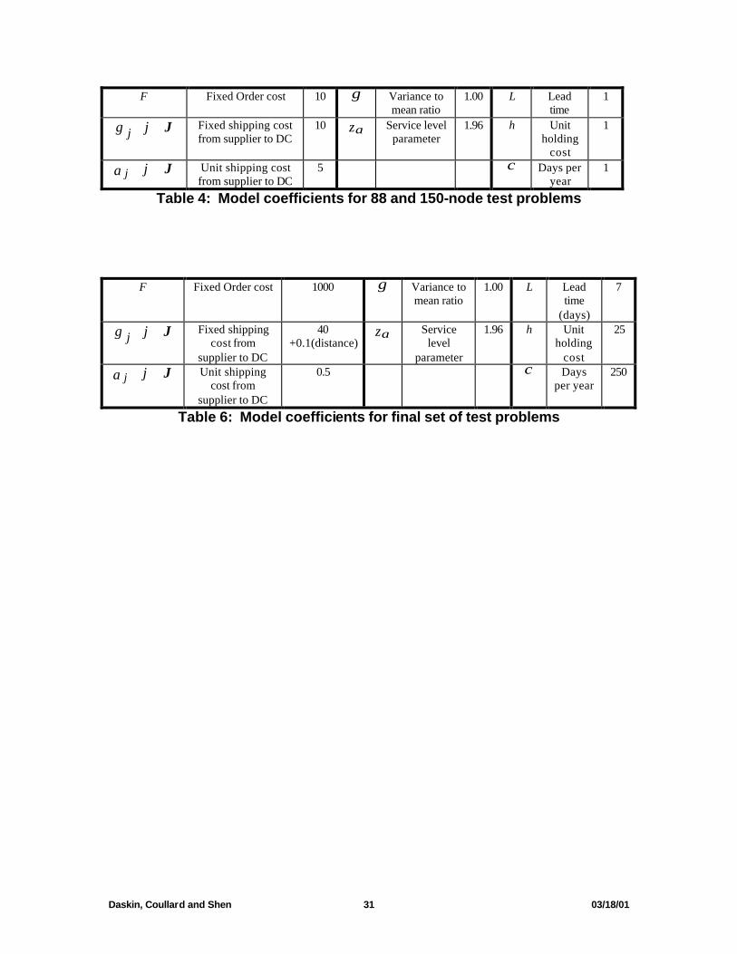
Table 4 presents the coefficients used in all the runs for both datasets.

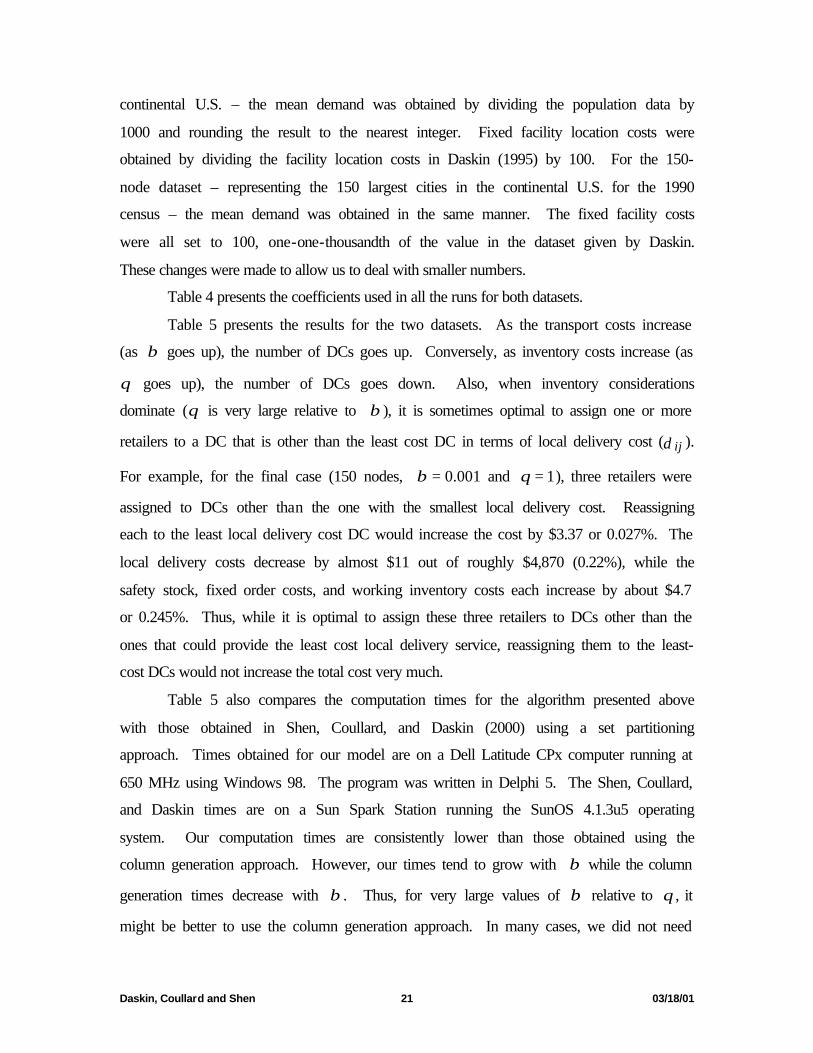
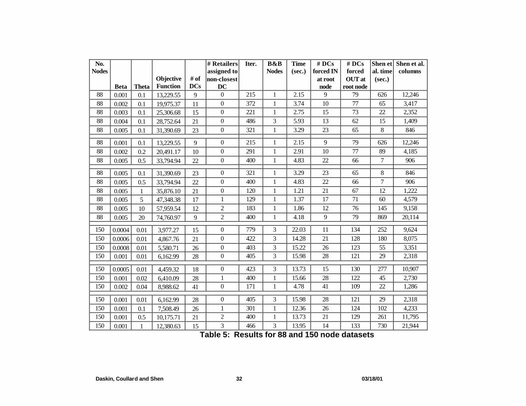
Table 5 presents the results for the two datasets. As the transport costs increase

(as β goes up), the number of DCs goes up. Conversely, as inventory costs increase (as

θ goes up), the number of DCs goes down. Also, when inventory considerations

dominate (θ is very large relative to β ), it is sometimes optimal to assign one or more

retailers to a DC that is other than the least cost DC in terms of local delivery cost (d ij ).

For example, for the final case (150 nodes, 001.0=β and 1=θ ), three retailers were

assigned to DCs other than the one with the smallest local delivery cost. Reassigning

each to the least local delivery cost DC would increase the cost by $3.37 or 0.027%. The

local delivery costs decrease by almost $11 out of roughly $4,870 (0.22%), while the

safety stock, fixed order costs, and working inventory costs each increase by about $4.7

or 0.245%. Thus, while it is optimal to assign these three retailers to DCs other than the

ones that could provide the least cost local delivery service, reassigning them to the least-

cost DCs would not increase the total cost very much.

Table 5 also compares the computation times for the algorithm presented above

with those obtained in Shen, Coullard, and Daskin (2000) using a set partitioning

approach. Times obtained for our model are on a Dell Latitude CPx computer running at

650 MHz using Windows 98. The program was written in Delphi 5. The Shen, Coullard,

and Daskin times are on a Sun Spark Station running the SunOS 4.1.3u5 operating

system. Our computation times are consistently lower than those obtained using the

column generation approach. However, our times tend to grow with β while the column

generation times decrease with β . Thus, for very large values of β relative to θ , it

might be better to use the column generation approach. In many cases, we did not need


to use branch and bound at all; when we did very few nodes deeded to be evaluated.

Finally, the variable forcing rules were exceptionally effective, forcing almost all nodes

in or out of the solution at the root node. This is in part due to the very tight bounds

obtained at the root node.

Finally, we consider a different variant of the 150-node dataset given in Daskin

(1995). In this case, we divided the demands by 250 and truncated the result to obtain the

mean daily demand. Table 6 gives the model coefficients for this set of runs, which were

designed to better replicate real-world conditions. Two supplier locations were

considered – Chicago and Phoenix – and the fixed shipping cost from the supplier to a

candidate DC was taken to be function of the distance from the closer supplier to the

candidate DC site as shown in Table 9.

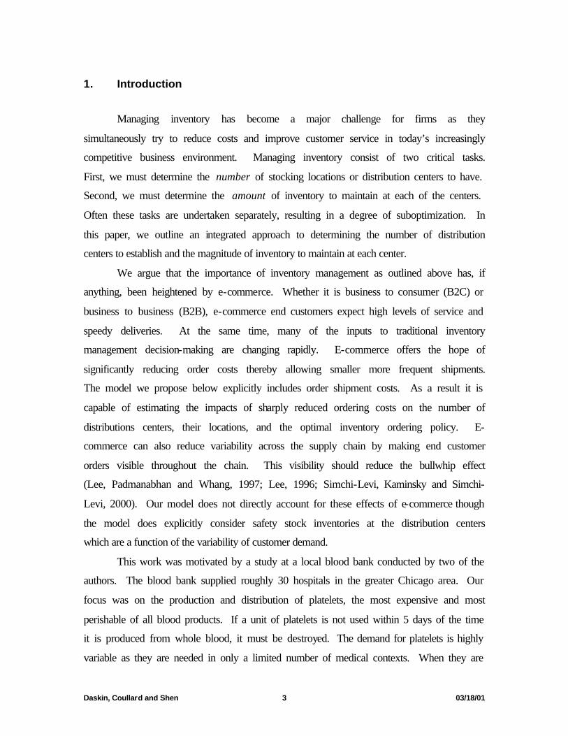
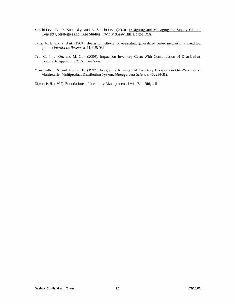
Figure 3 shows the optimal solution for a base case of 00025.0=β and 1.0=θ .

The supplier in Chicago serves 6 of the 10 DCs and about 73% of the total demand.

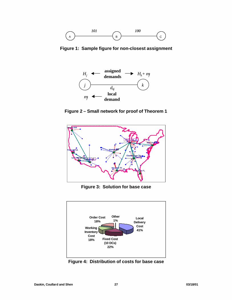
Figure 4 breaks down the total cost of approximately $4.49 million into its constituent

parts. Note that in this case, the transport costs from the suppliers to the DCs as well as

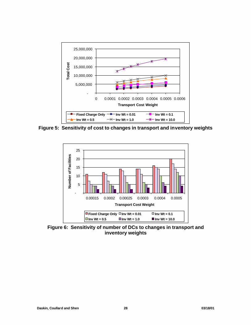
the safety stock costs – all buried in the “other” category – are negligible. Figures 5 and

6 show the sensitivity of the cost and number of facilities to changes in the transport and

inventory cost weights. As the relative importance of inventory costs goes up, the

number of DCs located goes down and as the importance of transport costs goes up, the

number of DCs increases. The figures also compare this model with the traditional

uncapacitated fixed charge (UFC) location model. Not surprisingly, the total cost for the

UFC model is always below that of the model presented above which includes additional

cost components. Also, due to the concavity of the additional cost terms, the UFC

consistently locates more DCs than does the model above.

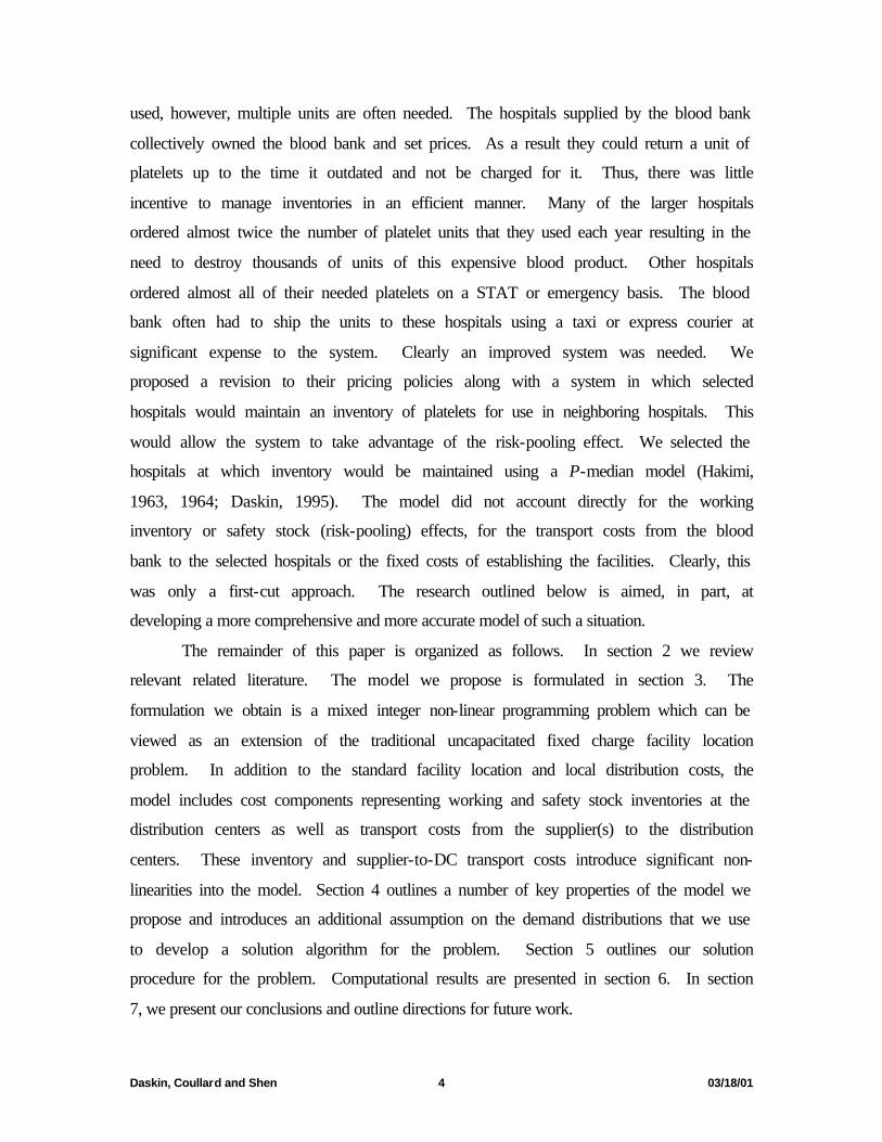
Finally, we consider how the solution might change if the fixed cost of placing an

order decreased significantly from $1000 per order to $10 per order as might be the case

with e-commerce technologies. The total cost decreases from $4.49 million to $2.9

million. Interestingly, it is now optimal to open 14 DCs instead of the 10 found in the

base case. This is reassuring since the demand-weighted average local delivery distance

to a retailer from a DC will decrease from 127.1 to 88.8 miles. It is reassuring that the

average distance decreases in this case, since e-commerce is often associated with


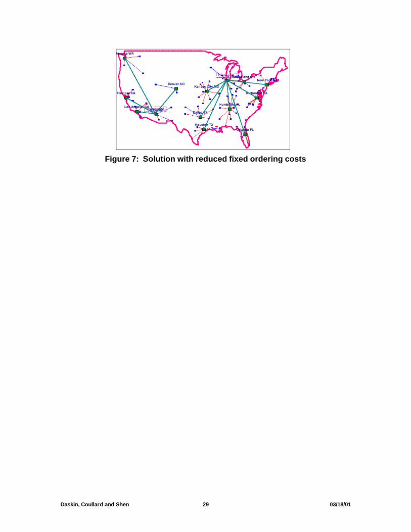
expectations of improved customer service. Figure 7 shows the new solution. The

supplier in Chicago serves 9 of the DCs and about 71% of the demand. Compared to the

cost breakdown in the base case (Figure 4), in this case, 48% of the total cost is in facility

costs and another 44.3% is in local delivery costs. Order costs and working inventory

costs each constitute 3.3% of the total costs while safety stock costs and shipment costs

from the supplier to the DCs are again negligible.

If we could not relocate or add to the set of open DCs used in the base case, but

could simply reoptimize the retailer assignments and inventory management policies, the

costs would be 4.1% higher than those for the solution shown in Figure 7. If we were

constrained to using the 10 DCs in the base case, but could add DCs, it would be optimal

to use 3 additional DCs located in Cleveland, OH, Denver, CO, and Richomond, VA.

The total cost in this case is only 1.1% greater than that of the optimal solution in Figure

7.

7. Conclusions and directions for future work

We have presented a new facility location model that incorporates working and

safety stock inventory costs at the distribution centers as well as the economies of scale

that exist in the transport costs from suppliers to DCs. A Lagrangian solution algorithm

was presented for the case in which the ratio of the variance of demand at the retailers to

the mean demand is the same for all retailers. A number of improvement heuristics were

outlined for the problem. Also, two variable forcing rules that are applied at the root

node of the branch and bound tree were discussed.

The algorithm was tested on two datasets consisting of 88 and 150 nodes

respectively. The computational results compare favorably with those of the set

partitioning approach proposed by Shen (2000) and Shen, Coullard and Daskin (2000).

In many cases, branch and bound was not needed because the bounds at the root node

proved the optimality of the solution and/or because we could force all of the candidate

DCs into or out of the solution. In a final set of tests, we included explicit supplier

locations and modified the inputs to better reflect actual conditions. When fixed order

costs are significantly reduced, the number of facilities located increases. Despite our


best efforts to reflect realistic conditions, it is important to test the data with actual

corporate data to confirm that the model is accurately capturing the relevant costs.

A number of extensions should be considered. First, we need to develop ways of

solving the problem when the ratio of the variance to the mean is not identical for all

retailers. Second, we hope to consider the cases with multiple items as well as a

constraint on the maximum allowable inventory at a DC and a constraint on the

maximum demand that can be served by a supplier. Finally, it might be possible to

incorporate local delivery cost estimates that better reflect less-than-truckload routing

since such approximations often involve the square root of demand (Daganzo, 1991). We

are working in all of these areas.

References

Balinski, M. (1965). Integer programming: Methods, uses, computation. Management Science, 13, 253-313.

Berger, R. T., C. R. Coullard, M. S. Daskin (1998). Modeling and Solving Location-Routing Problems with Route-Length Constraints. Working Paper, Northwestern University.

Berman, O., P. Jaillet and D. Simchi-Levi (1995). Location-Routing Problems with Uncertainty. Facilities Location, Z. Drezner ed., Springer Verlag, 427--452.

Chan, L. M. A., A. Federgruen and D. Simchi-Levi (1998). Probabilistic Analysis and Practical Algorithms for Inventory Routing Models . Operations Research, 46, 96--106.

Daganzo, C., (1991). Logistics Systems Analysis , Lecture Notes in Economics and Mathematical Systems, M. Beckmann and W. Krelle eds., Springer Verlag, Berlin.

Daskin, M. S. (1995). Network and Discrete Location: Models, Algorithms, and Applications, John Wiley and Sons, NY.

Daskin, M. S., and S. H. Owen (1999). Location Models in Transportation. In Handbook of Transportation Science, R. Hall ed., Kluwer Academic Publishers, Norwell, MA, 311-360.

Drezner, Z., editor (1995). Facility Location: A survey of Applications and Methods, Springer, NY.

Erlebacher, S. J. and R. D. Meller (2000). The interaction of location and inventory in designing distribution systems. IIE Transactions, 32, 155-166.

Erlenkotter, D. (1978). A dual-based procedure for uncapacitated facility location. Operations Research, 14, 361-368.

Eppen, G. (1979). Effects of Centralization on Expected Costs in a Multi-Location Newsboy Problem. Management Science 25, No. 5, 498-501.


Federgruen, A. and D. Simchi-Levi (1995), Analytical Analysis of Vehicle Routing and Inventory Routing problems. Handbooks in Operations Research and Management Science, the volume on Network Routing. M. Ball, T. Magnanti, C. Monma and G. Nemhauser, eds., North-Holland, Amsterdam, 297-373

Federgruen, A. and P. Zipkin (1984), A combined Vehicle Routing and Inventory Allocation Problem, Management Science, 32, 1019-1036.

Fisher, M. L. (1981). The Lagrangian relaxation method for solving integer programming problems. Management Science, 27, 1-18.

Fisher, M. L. (1985). An applications oriented guide to Lagrangian relaxation. Interfaces, 15:2, 2-21.

Graves, S. C., A. H. G. Rinnooy Kan and P. H. Zipkin (1993). Logistics of Production and Inventory, Elsevier Science Publishers, Amsterdam, The Netherlands.

Hakimi S. (1965). Optimum location of switching centers in a communications network and some related graph theoretic problems. Operations Research, 13, 462-475.

Hakimi S. (1964). Optimum location of switching centers and the absolute centers and medians of a graph. Operations Research 12, 450-459.

Kleywegt, A.J., Nori, V.S., and Savelsbergh, M.W.P. (2000). The Stochastic Inventory Routing Problem, working paper, Georgia Institute of Technology.

Korkel, M. (1989). On the exact solution of large-scale simple plant location problems. European Journal of Operations Research, 39, 157-173.

Laporte, G., P. J. Dejax (1989). Dynamic Location-Routing Problems. Journal of Operations Research Society, 40, No.5, 471-482

Lee, H., V. Padmanabhan, and S. Whang. (1997) The Bullwhip Effect in Supply Chains. Sloan Management Review, Spring, 93-102.

Lee, H. (1996) Information Distortion in a Supply Chain: The Bullwhip Effect. Management Science, 43, 546-558.

Montgomery, D. C., G. C. Runger, and N. F. Hubele, (1998). Engineering Statistics, John Wiley, NY.

Nahmias, S. (1997). Production and Operations Management, Third Edition, Irwin, Chicago.

Owen, S. H., and M. S. Daskin (1998). Strategic Facility Location: A Review. European Journal of Operational Research, 111, 423-447.

Sheffi, Y., (1985). Urban Transportation Networks: Equilibrium Analysis with Mathematical Programming Methods, Prentice Hall, Englewood Cliffs, NJ.

Shen, Z. J. (2000) Efficient Algorithms for Various Supply Chain Problems, Ph.D. Dissertation, Department of Industrial Engineering and Management Sciences, Northwestern University, Evanston, IL 60208.

Shen, Z. J., C. R. Coullard, and M. S. Daskin (2000) A Joint Location-inventory Model, submitted to Transportation Science.


Simchi-Levi, D., P. Kaminsky, and E. Simchi-Levi, (2000). Designing and Managing the Supply Chain: Concepts, Strategies and Case Studies, Irwin McGraw Hill, Boston, MA.

Teitz, M. B. and P. Bart. (1968). Heuristic methods for estimating generalized vertex median of a weighted graph. Operations Research, 16, 955-961.

Teo, C. P., J. Ou, and M. Goh (2000). Impact on Inventory Costs With Consolidation of Distribution Centers, to appear in IIE Transactions.

Viswanathan, S. and Mathur, K. (1997), Integrating Routing and Inventory Decisions in One-Warehouse Multiretailer Multiproduct Distribution System, Management Science, 43, 294-312.

Zipkin, P. H. (1997). Foundations of Inventory Management, Irwin, Burr Ridge, IL.


A B C101 100

A B C101 100

Figure 1: Sample figure for non-closest assignment

j k

Hj Hk+ µjassigneddemands

µjlocal

demand

dkj

Figure 2 – Small network for proof of Theorem 1

Figure 3: Solution for base case

Local Delivery

Cost41%

Fixed Cost (10 DCs)

22%

Working Inventory

Cost18%

Order Cost18%

Other1%

Figure 4: Distribution of costs for base case


-

5,000,000

10,000,000

15,000,000

20,000,000

25,000,000

0 0.0001 0.0002 0.0003 0.0004 0.0005 0.0006

Transport Cost Weight

Tota

l Cos

t

Fixed Charge Only Inv Wt = 0.01 Inv Wt = 0.1Inv Wt = 0.5 Inv Wt = 1.0 Inv Wt = 10.0

Figure 5: Sensitivity of cost to changes in transport and inventory weights

-

5

10

15

20

25

0.00015 0.0002 0.00025 0.0003 0.0004 0.0005

Transport Cost Weight

Num

ber o

f Fac

ilitie

s

Fixed Charge Only Inv Wt = 0.01 Inv Wt = 0.1Inv Wt = 0.5 Inv Wt = 1.0 Inv Wt = 10.0

Figure 6: Sensitivity of number of DCs to changes in transport and

inventory weights


Figure 7: Solution with reduced fixed ordering costs


NODE A B C Fixed Cost 10 1000 10 Mean 100 1 1 Table 1a: Data for network in Figure 1

F Fixed Order cost 10 β Transport weight

1 L Lead time

1

J∈∀jg j Fixed shipping cost from supplier to DC

1 zα Service level parameter

1.96 h Unit holding

cost

2

J∈∀ja j Unit shipping cost from supplier to DC

1 θ Inventory weight

1 χ Days per year

1

Table 1b: Parameters for network in Figure 1 Retailer Assignments

Facilities A B C Facility

cost

Local Delivery

Cost Inventory

Cost Total Cost Cost - min

cost A A A A 10 304 106.58 420.58 181.97 B B B B 1,000 10,301 106.58 11,407.58 11,168.97 C C C C 10 20,301 106.58 20,417.58 20,178.97

A,C A C C 20 101 120.46 241.46 2.84 A,C A A C 20 102 116.61 238.61 0.00 A,B A B B 1,010 101 120.46 1,231.46 992.84

A,B,C A B C 1,020 0 126.64 1,146.64 908.03 Table 2: Costs of different DC locations and retailer assignments

Parameter Value Maximum number of iterations 400 Minimum alpha multiplier 0.00000001 Maximum number of iterations before halving alpha 12 Crowder’s damping factor 0.3 Initial Lagrange multiplier value f j1010 +µ

Table 3: Parameters for Lagrangian relaxation runs


F Fixed Order cost 10 γ Variance to mean ratio

1.00 L Lead time

1

J∈∀jg j Fixed shipping cost from supplier to DC

10 zα Service level parameter

1.96 h Unit holding

cost

1

J∈∀ja j Unit shipping cost from supplier to DC

5 χ Days per year

1

Table 4: Model coefficients for 88 and 150-node test problems

F Fixed Order cost 1000 γ Variance to mean ratio

1.00 L Lead time

(days)

7

J∈∀jg j Fixed shipping cost from

supplier to DC

40 +0.1(distance)

zα Service level

parameter

1.96 h Unit holding

cost

25

J∈∀ja j Unit shipping cost from

supplier to DC

0.5 χ Days per year

250

Table 6: Model coefficients for final set of test problems


No. Nodes

Beta Theta Objective Function

# of DCs

# Retailers assigned to non-closest

DC

Iter. B&B Nodes

Time (sec.)

# DCs forced IN

at root node

# DCs forced OUT at

root node

Shen et al. time (sec.)

Shen et al. columns

88 0.001 0.1 13,229.55 9 0 215 1 2.15 9 79 626 12,246 88 0.002 0.1 19,975.37 11 0 372 1 3.74 10 77 65 3,417 88 0.003 0.1 25,306.68 15 0 221 1 2.75 15 73 22 2,352 88 0.004 0.1 28,752.64 21 0 486 3 5.93 13 62 15 1,409 88 0.005 0.1 31,390.69 23 0 321 1 3.29 23 65 8 846

88 0.001 0.1 13,229.55 9 0 215 1 2.15 9 79 626 12,246 88 0.002 0.2 20,491.17 10 0 291 1 2.91 10 77 89 4,185 88 0.005 0.5 33,794.94 22 0 400 1 4.83 22 66 7 906

88 0.005 0.1 31,390.69 23 0 321 1 3.29 23 65 8 846 88 0.005 0.5 33,794.94 22 0 400 1 4.83 22 66 7 906 88 0.005 1 35,876.10 21 0 120 1 1.21 21 67 12 1,222 88 0.005 5 47,348.38 17 1 129 1 1.37 17 71 60 4,579 88 0.005 10 57,959.54 12 2 183 1 1.86 12 76 145 9,158 88 0.005 20 74,760.97 9 2 400 1 4.18 9 79 869 20,114

150 0.0004 0.01 3,977.27 15 0 779 3 22.03 11 134 252 9,624 150 0.0006 0.01 4,867.76 21 0 422 3 14.28 21 128 180 8,075 150 0.0008 0.01 5,580.71 26 0 403 3 15.22 26 123 55 3,351 150 0.001 0.01 6,162.99 28 0 405 3 15.98 28 121 29 2,318

150 0.0005 0.01 4,459.32 18 0 423 3 13.73 15 130 277 10,907 150 0.001 0.02 6,410.09 28 1 400 1 15.66 28 122 45 2,730 150 0.002 0.04 8,988.62 41 0 171 1 4.78 41 109 22 1,286

150 0.001 0.01 6,162.99 28 0 405 3 15.98 28 121 29 2,318 150 0.001 0.1 7,508.49 26 1 301 1 12.36 26 124 102 4,233 150 0.001 0.5 10,175.71 21 2 400 1 13.73 21 129 261 11,795 150 0.001 1 12,380.63 15 3 466 3 13.95 14 133 730 21,944

Table 5: Results for 88 and 150 node datasets

Documents

An Inventory-Location Model: Formulation, Solution ... · Formulation, Solution Algorithm and Computational ... We argue that the importance of inventory management ... inventory