Copyright © 2008, 2009, 2010 by Craig J. Chapman and Thomas J. Steenburgh

Working papers are in draft form. This working paper is distributed for purposes of comment and discussion only. It may not be reproduced without permission of the copyright holder. Copies of working papers are available from the author.

An Investigation of Earnings Management through Marketing Actions Craig J. Chapman Thomas J. Steenburgh

Working Paper

08-073

AN INVESTIGATION OF EARNINGS MANAGEMENT

THROUGH MARKETING ACTIONS1

Craig J. Chapman2, Thomas J. Steenburgh

3

Harvard Business School Working Paper, No. 08-073

Draft July 16, 2010

Abstract:

Prior research hypothesizes managers use „real actions,‟ including the reduction

of discretionary expenditures, to manage earnings to meet or beat key benchmarks. This

paper examines this hypothesis by testing how different types of marketing expenditures

are used to boost earnings for a durable commodity consumer product which can be

easily stockpiled by end-consumers.

Combining supermarket scanner data with firm-level financial data, we find

evidence that differs from prior literature. Instead of reducing expenditures to boost

earnings, soup manufacturers roughly double the frequency and change the mix of

marketing promotions (price discounts, feature advertisements and aisle displays) at the

fiscal quarter-end when they have greater incentive to boost earnings.

1 We thank the James M. Kilts Center, GSB, University of Chicago for data used in this study and also

Dennis Chambers, Paul Healy, VG Narayanan, two anonymous referees and seminar participants at the

Harvard Business School, the Massachusetts Institute of Technology, the London Business School

Transatlantic Conference and the AAA FARS 2007 Conference for their helpful comments on the paper. 2 Kellogg School of Management, Northwestern University, c-chapman@kellogg.northwestern.edu

3 Harvard Business School

2

Our results confirm managers‟ stated willingness to sacrifice long-term value in

order to smooth earnings (Graham, Harvey and Rajgopal, 2005) and their stated

preference to use real actions to boost earnings to meet different types of earnings

benchmarks. We estimate that marketing actions can be used to boost quarterly net

income by up to 5% depending on the depth and duration of promotion. However, there

is a price to pay, with the cost in the following period being approximately 7.5% of

quarterly net income.

Finally, a unique aspect of the research setting allows tests of who is responsible

for the earnings management. While firms appear unable to increase the frequency of

aisle display promotions in the short run, they can reallocate these promotions within

their portfolio of brands. Results show firms shifting display promotions away from

smaller revenue brands toward larger ones following periods of poor financial

performance. This indicates the behavior is determined by parties above brand managers

in the firm.

These findings are consistent with firms engaging in real earnings management

and suggest the effects on subsequent reporting periods and competitor behavior are

greater than previously documented.

3

1. Introduction

Degeorge, Patel and Zeckhauser (1999) propose that earnings management behavior can

be divided into two distinct categories:

“misreporting” earnings management – involving merely the discretionary accounting

of decisions and outcomes already realized; and

“direct” or “real” earnings management - the strategic timing of investment, sales,

expenditures and financing decisions.

In this paper, we observe an example of “real” earnings management. We present

evidence of managers deviating from their normal business practices depending on their

firms‟ fiscal calendars and financial performance. These managers increase the

frequency and change the mix of retail-level marketing actions (price discounts, feature

advertisements, and aisle displays) to influence the timing of consumers‟ purchases to

manage reported earnings.

In the marketing literature, there are numerous papers studying how price discounts and

other marketing actions affect customer buying behavior. Some marketing actions, such

as television advertising, have a limited impact on short-term performance, but result in

greater brand equity over time. Such actions are similar to research and development

expenditures, as the benefits accrue long after the investment is made. In contrast, retail

marketing actions such as price discounts, feature advertisements and aisle displays,4

boost short-term performance while they are run, but bring little or no positive long-term

4 Commonly referred to as „sales promotions‟

4

benefits to the brand. In fact, sales promotions often induce customer stockpiling which

leads to a drop in sales in the period right after they are run, a phenomenon referred to as

the “post-promotion dip” in the marketing literature.

Although marketing can be used tactically in response to changing demand conditions,

the vast literature on both accounting and real earnings management suggests they might

also be used to manage earnings. A limited amount of prior research has examined how

firms reduce marketing expenditures when seeking to boost earnings in the short-term.

These studies, however, have focused on reductions in advertising expenditures, which

sacrifice value far in the future.5 In contrast, we provide evidence that managers increase

other types of marketing expenditures in order to boost earnings in the short-term, using

sales promotions to induce customer stockpiling.6 Thus, firms are willing to bear an

immediate cost to shift income across time periods.

We base our study on a widely used dataset that tracks the retail promotional activities

for soup, a relatively durable good that consumers are willing to stockpile,7 and we add to

these data by hand collecting information about the soup manufacturers‟ financial

performance and related analyst forecasts. We begin by showing how promotional

activities observed in retail stores relate to soup manufacturers‟ fiscal calendars and

earnings management incentives. We find that soup manufacturers increase the

frequency and change the mix of marketing promotions when they need to meet earnings

5 For example, see Mizik and Jacobson (2007) who find that firms reduce marketing expenditures prior to

seasoned public offerings to boost short-term earnings or Cohen, Mashruwala and Zach (2009) who find

that managers reduce their advertising spending to achieve the financial reporting goals. 6 This behavior is consistent with Stein‟s (1989) myopic behavior model or the “borrowing of earnings”

discussed by Degeorge, Patel and Zeckhauser (1999). 7 See Narasimhan, Neslin and Sen (1996) and Pauwels, Hanssens and Siddarth (2002) for discussion of

stockpiling ease.

5

targets. Specifically, manufacturers that: have just experienced small quarterly earnings

decreases (year-on-year) in the prior quarter; report a small increase in year-on-year

quarterly earnings for the current quarter; or report earnings that just beat analyst

consensus forecasts are more likely to offer products at special prices or run specific

promotions (including less attractive unsupported price promotions) towards the end of

fiscal periods as they have greater incentive to increase short term earnings.

The willingness of firms to use marketing actions in this manner was evidenced in a

recent statement by Douglas R. Conant, President and Chief Executive Officer of

Campbell Soup Company during their quarterly earnings conference call “We then

managed our marketing plans to manage our [earning]8” (Campbell Soup Company,

2008).

A unique aspect of our research setting allows us to test who is responsible for the

earnings management. While it is very difficult for firms to immediately increase the

frequency of display promotions, they can readily reallocate these promotions within

their portfolio of brands. We observe that firms switch their promotional slots from

smaller revenue brands to larger brands in periods when we predict them to have

incentives to manage earnings upwards. Since it is highly unlikely that a brand manager

would voluntarily give up promotional support, this change is consistent with the actions

being directed, at least in part, by parties higher in the organization than the brand

managers.

8 The word “earning” can be clearly heard at time 33:40 in the audio version of the conference call but has

been redacted from the call transcript available at http://seekingalpha.com/article/77913-campbell-soup-

f3q08-qtr-end-4-27-08-earnings-call-transcript?page=-1

6

2. Hypothesis Development

There have been many papers in the accounting and finance literature studying earnings

management. Early examples include: Healy (1985) who asserts that accrual policies of

managers are related to income-reporting incentives of their bonus contracts; Hayn

(1995) who asserts firms whose earnings are expected to fall just below zero engage in

earnings manipulations to help them cross the „red line‟ for the year; and Burgstahler and

Dichev (1997) who more generally find that firms manage earnings opportunistically to

meet thresholds.9

Healy and Wahlen (1999) report that early research on earnings management mostly

considered whether and when earnings management takes place by examining broad

measures of earnings management (i.e. measures based on total accruals). They noted

several studies of firms managing earnings using specific accruals which fall neatly into

the “misreporting” category of earnings management proposed by Degeorge, Patel and

Zeckhauser (1999).

More recent work by Graham, Harvey and Rajgopal (2005) provides support for

arguments that managers also use “real” earnings management techniques. Not only do

they find that the majority of managers surveyed (78%) admit to taking actions that

sacrifice long-term value to smooth earnings, but they also find that managers prefer to

use real actions over accounting actions to meet earnings benchmarks. In a similar vein,

9 Durtschi and Easton (2005) suggest that the shapes of the frequency distributions of earnings metrics at

zero cannot be used as ipso facto evidence of earnings management and are likely due to the combined

effects of deflation, sample selection, and differences in the characteristics of observations to the left of

zero from those to the right.

7

Roychowdhury (2006) asserts that managers select operational activities which deviate

from normal business practices to manipulate earnings and meet earnings thresholds.

How might marketing actions be used to boost earnings? Suppose a manager runs a

short-term promotion to lift sales volume; if the associated increase in net revenue

exceeds the cost of the promotion, short-term profits also rise. This raises the question of

why the promotion is not run regularly. In the case of durable goods, at least some of the

incremental sales are due to consumer stockpiling, which leads to subsequent reduced

sales.10

Thus, overall profits may actually fall, despite the current period gains.

2.1. The Relation between Financial Performance, the Fiscal Calendar and

Promotions

Past literature suggests multiple circumstances in which managers may change behavior

when they have incentive to manage earnings upwards.11

Although price discounting

may lead to customer stockpiling, some have proposed that firms reduce prices towards

the end of reporting periods to smooth or boost earnings.12

Provided that demand is sufficiently elastic to boost short-term earnings (which we show

to be the case in section 4.6), managers may use price reductions to boost sales and

earnings just prior to the end of the fiscal quarter (year). We therefore propose the

following hypothesis:

10

See Macé and Neslin (2004) and Van Heerde et al. (2004) for discussion of the post-promotion dip. 11

See Healy (1985), Jones (1991), Burgstahler and Dichev (1997) and Bushee (1998) for general examples. 12

See Fudenberg and Tirole (1995), Oyer (1998) and Roychowdhury (2006) .

8

H1 During the final month of a manufacturer’s fiscal quarter (year), special price

discounts will occur more frequently and the depth of these discounts will be

greater for manufacturers expected to be managing earnings upwards.

Other authors have focused on the strategic reduction of discretionary spending prior to

financial reporting deadlines. Graham, Harvey and Rajgopal (2005) find that 80% of

survey respondents report they would decrease discretionary spending on R&D,

advertising, and maintenance to meet an earnings target. Roychowdhury (2006) finds

evidence of firms reducing discretionary spending to avoid losses. Dechow and Sloan

(1991), Bushee (1998) and Cheng (2004) draw similar conclusions and show changes in

R&D expenditure to be systematically related to reported earnings. Focusing exclusively

on advertising and marketing expenditures, Mizik and Jacobson (2007) observe

reductions in marketing expenditures at the time of seasoned equity offerings and Cohen,

Mashruwala and Zach (2009) find that managers reduce their advertising spending to

achieve the financial reporting goals.

We should not conclude from this literature, however, that firms reduce all marketing

expenditures prior to financial reporting deadlines. The benefits from different types of

expenditures are realized over vastly different time horizons. Television advertising

investments build the long-term equity of a brand, but typically have little impact on

short-term sales. Therefore, firms may reasonably choose to reduce this type of spending

in order to meet short-term goals. In contrast, sales promotions, including price

reductions, feature advertisements and aisle display promotions, can have a dramatic and

9

measurable short-term impact on sales. Firms may therefore choose to increase this type

of spending in order to meet short-term goals.

In describing the difference between television advertising and sales promotions, Aaker

(1991) notes:

It is tempting to “milk” brand equity by cutting back on brand-building activities, such as

[television] advertising, which have little impact on short-term performance. Further,

declines in sales are not obvious. In contrast, sales promotions, whether they involve

soda pop or automobiles, are effective – they affect sales in an immediate and measurable

way. During a week in which a promotion is run, dramatic sales increases are observed

for many product classes: 443% for fruit drinks, 194% for frozen dinners, and 122% for

laundry detergents.

In spite of these differences, we are unaware of any research that demonstrates how the

timing and frequency of sales promotions relate to the fiscal calendar. Given that our

research setting is a highly durable good with relatively low storage costs where

stockpiling is likely, we propose the following hypothesis:

H2 During the final month of a manufacturer’s fiscal quarter (year), feature and

display promotions will occur more frequently for manufacturers expected to be

managing earnings upwards.

We predict that firms and managers have stronger incentive to manage earnings upwards

when the firm is seeking to meet or beat the EPS figure from the same quarter in the

previous year and when the firm reports (ex-post) earnings that just beat analyst

consensus estimates.13

We base these predictions, in part, on Graham, Harvey and

Rajgopal (2005), who find these the two most important earnings benchmarks in their

survey, with 85.1% and 73.5% of respondents citing them, respectively.

13

We thank the anonymous referee for proposing the inclusion of the analyst consensus forecasts.

10

Evidence confirming the previous two hypotheses would be consistent with the “strategic

timing of investment, sales, expenditures and financing decisions” part of Degeorge,

Patel and Zeckhauser‟s (1999) definition of earnings management. However, our

research setting also permits estimation of the costs and benefits of promotions being run

in different combinations. In line with prior literature, we show that special price

promotions are most effective when offered with feature advertisement and aisle display

promotions. 14

Not surprisingly, therefore, we observe special price promotions

frequently supported by contemporaneous feature and/or display promotions. However,

we also observe unsupported (and less effective) price promotions.15

Industry experts have told us that display promotions are usually scheduled several

months in advance and it is very difficult for firms to increase their frequency at short

notice. This means that price promotions planned at short notice are less likely to be

supported with display promotions. We therefore test the following hypothesis:

H3 During the final month of a manufacturer’s fiscal quarter (year), unsupported

special price discounts will occur more frequently and the depth of these

discounts will be greater for manufacturers expected to be managing earnings

upwards.

14

See Hypotheses H7 and H8 in Mela, Gupta and Lehmann (1997) for example. 15

Approximately ⅔ of special price promotions are supported with a feature advertisement and ⅓ are

supported with an aisle display with 15% being unsupported altogether.

11

2.2. Who is Behind the Earnings Management Behavior?

Our research also sheds light on a question that prior literature has found difficult to

answer: who within the organization is responsible for the earnings management

behavior?

Healy (1985) suggests that it is the managers who select accounting procedures and

accruals that have the incentives to maximize the value of their bonus awards and will

therefore use their discretion to manage earnings. Oyer (1998) finds results consistent

with both upper management and salespeople affecting fiscal seasonality. However, he

clearly states that his results do not prove that top management is the main cause of the

fiscal-year effects, nor does he make a clear distinction between the roles of managers

and salespeople.

Oberholzer-Gee and Wulf (2006), using various measures of earnings manipulation

including discretionary accounting accruals, show that higher-powered incentives for

division managers can lead to greater accounting manipulation than similar changes for

CEOs. This work points more towards divisional managers than CEOs being responsible

for earnings manipulation.

The question of who is responsible for allocating marketing resources has not been

answered in the marketing literature either. As discussed in Blattberg and Neslin (1990),

corporate and division objectives serve as the starting point for planning all marketing

activities and senior managers are taking a more active role in this area.16

However, the

establishment of a total marketing budget requires negotiation between both brand

16

Blattberg and Neslin (1990) p.382

12

managers and senior management.17

This suggests that national brand managers and

other senior executives are responsible for deciding which of the brands within the

company are promoted and when these promotions occur, not lower-level managers.

This was confirmed during unstructured interviews with representatives of multiple

durable goods manufacturers. During these discussions, it became apparent that large

promotions generally need explicit C-level executive approval.

In our research setting, we are able to examine differences in promotion activity within

each sample firm by considering how promotion behavior differs based upon the

importance of a brand to the company and the importance of a product within a brand as

measured by their relative revenue contributions. This allows us to test the following

hypotheses:

H4 In the final month of the fiscal year when manufacturers are expected to be

managing EPS upwards, prices will be cut more for: a) higher revenue UPC

codes within a brand; and b) higher revenue brands within a manufacturer.

While evidence in favor of these hypotheses may provide interesting information about

manager selectivity in price promotion, it is unlikely to answer who in the organization is

responsible for these decisions since both the CEO and the brand managers are likely to

have incentives to take these pricing actions.

Nevertheless, our data also contain information about the frequency of display

promotions. Industry experts have told us that display promotions are usually scheduled

several months in advance and it is very difficult for firms to increase their frequency at

17

Blattberg and Neslin (1990) p.391

13

short notice. Yet, it is possible for firms to switch their display promotions within their

own suite of brands. Using a sub-sample of our data which contains only products with

multiple UPC codes within each brand and also multiple brands within each

manufacturer, we test the following hypotheses:

H5 In the final month of the fiscal year of manufacturers expected to be managing

EPS upwards, display promotions will occur more frequently for: a) higher

revenue UPC codes within a brand; and b) higher revenue brands within a

manufacturer.

As with the previous hypotheses, it is difficult to draw conclusions as to responsibility if

we simply observe an increase in promotion for the higher revenue UPC codes within

brands or brands within manufacturers. However, if we observe promotions switching

from lower revenue brands to higher revenue brands, we propose that senior managers

are making the decisions. All brand managers would like to increase their display

promotions, but only some are allowed to do so while others are forced to reduce theirs.

3. Data and Methodology

The data used in this study were collected between 1985 and 1988 by the ERIM

marketing testing service. The data contain the purchase patterns of 2,500 households in

Sioux Falls, SD and Springfield, MO. These data have been widely studied in the past

and can be downloaded from the University of Chicago Graduate School of Business

website.18

18

http://research.chicagogsb.edu/marketing/databases/dominicks/index.aspx.

14

We chose to base our study on the use of promotions in the soup product category. Prior

research by Narasimhan, Neslin and Sen (1996) and Hanssens, Pauwels, and Siddarth

(2002) shows that soup is easily stockpiled and is purchased in greater quantities when it

is offered at a discount. Therefore, the hypothesized earnings management behavior

should be observable here.

For each individual UPC code (product), we expanded the dataset by identifying the

product producer and ultimate parent company. We then hand collected information

regarding the financial performance of these companies from multiple sources including

Thompson Financial, Corporate Websites, Compustat and One Source. When these data

were unavailable from public sources, we contacted the companies directly seeking to

obtain the information required. We were able to obtain these data regarding 38 different

brands (out of the 50 that we can identify in the full dataset) representing 27 distinct

manufacturers. Analyst forecasts were obtained from Zacks Investment Research

database (adjusted for stock splits) with the consensus estimate calculated as the mean of

the last forecast of the fiscal quarter‟s earnings made by each analyst prior to the

beginning of the quarter and not more than one year prior to the end of the quarter.

Table 1 shows summary statistics of our dataset which contains a total of over 233,000

individual item purchases from 36 different stores. From these, we are able to identify

the manufacturer for just over 200,000 observations (85.7%) and the fiscal calendar for

197,000 (84.5%). Given the significant market share garnered by Campbell‟s products in

the soup category (>80% in each of our sub-samples), we consider separately the effects

15

of Campbell‟s products in the data to ensure that the results are not being driven entirely

by this dominant player in the marketplace.

For the firms under consideration, the percentage of revenues associated with soup as

disclosed in their business segment report contained in the 10-K filing19

represents an

average of 52.5% of sales with a range of 2–100% and a standard deviation of 15.0%.

Due to concerns about lack of independence of observations within the dataset, we use a

single randomly selected observation for each product-week-store triplet. This allows us

to draw conclusions as to the probability of a promotion activity within a store for a

particular product. Collectively, these constraints restrict our sample to a total of 114,870

observations. Within this sample, the probability of a product being offered with some

form of promotion is 2.7% overall with the probability of a special price, feature or

display being 2.0%, 1.5% and 1.3% respectively.

We recognize that many products are never promoted during their lifecycle. To increase

test power, we therefore report additional results based upon a restricted sample of

products offered at a special price at some point during the observation period,

representing 38,262 observations. Within this sample, the probability of a product being

offered with some form of promotion is 7.6% overall with the probability of a special

price, feature or display being 5.9%, 4.5% and 3.3% respectively.

For tests of hypotheses H4 and H5, we use a sub-sample of our data which contains

multiple UPC codes within each brand and also multiple brands within each

manufacturer.

19

This often incorporates related businesses such as sauces and sometimes beverages.

16

As shown in figure 1, there is significant calendar seasonality of demand in the products

studied here. We therefore control for calendar month fixed effects and seek

identification for our regression models from the differences in fiscal calendars of the

companies manufacturing the products.20

This research design is similar to the one used

by Oyer (1998) and controls for seasonality of the data. In the event that a random

sample of competitors responded contemporaneously in a similar fashion to a promotion,

this would bias the coefficients of interest towards zero and against finding results.

Our interpretation of results is based upon the assumption that the supermarket chains are

passing through at least some of the discounts/promotions from the manufacturers as

opposed to selectively targeting specific months within each manufacturers‟ fiscal

calendars with their promotional activities.

We report t-statistics calculated using standard errors corrected for autocorrelation using

the Newey-West procedure for the OLS regressions21

and Huber-White adjusted standard

errors for the logistic regressions allowing for lack of independence between observations

for each product. Where quoted, pseudo-R2 is the McKelvey-Zavonia pseudo-R

2.22

20

The frequency distribution of fiscal year-ends is shown in figure 2. 21

Consistent with Stock and Watson (Eqn 13.17), we use a 4 week truncation parameter being estimated as

¾n⅓ where n is the number of weeks in the sample. Use of alternative truncation parameters does not

change the results materially. 22

The McKelvey-Zavonia pseudo-R2 is defined as var(ŷi) / [1+ var(ŷi)] where var(ŷi) is the variance of the

forecasts values for the latent dependent variable (Hagle and Mitchell (2001)).

17

4. Results and Discussion

4.1 Marketing Actions when Incentives to Manage Earnings Relating to Prior

Earnings Target and Analyst Earnings Forecasts are Higher

We first examine whether marketing actions are more likely to occur at the fiscal

Quarter-end (Year-end) than they are in other months for firms which we expect are more

likely to be managing EPS upwards. We examine behavior at the end of the fiscal

quarter because prior literature23

shows a significant post-promotion dip in sales occurs

right after a promotion is run. Running promotions early in reporting periods would not

be an effective way to manage earnings because some of their effects would reverse

before the period closed.

Based on Graham, Harvey and Rajgopal (2005), we predict that firms are more likely to

manage earnings upwards to meet or beat the EPS figure from the same quarter in the

previous year. We therefore consider how firms behave at the end of periods that

immediately follow quarters in which they have reported a small reduction in EPS

compared to the previous year. We predict these firms are more likely to experience a

small reduction in current period EPS compared to the previous year (absent any

Earnings Management) and may need to „catch up‟ the shortfall before the end of the

fiscal year and therefore have stronger incentive to manage earnings upwards. Graham,

Harvey and Rajgopal (2005) also suggest that managers have incentive to beat Consensus

Earnings Forecasts. We therefore predict that incentives to boost earnings are stronger

for firms which report (ex-post) earnings that just beat analyst consensus estimates.

23

See Macé and Neslin (2004) for example.

18

To test hypotheses H1 and H2, we estimate the following logistic regressions for each of

the three different marketing actions (special prices, feature advertisements or aisle

displays):

24

where Action is substituted by Special Price, Feature or Display, three dummy variables

which equal one if the sale is associated with a special price, feature or display promotion

respectively, zero otherwise. QuarterEnd (YearEnd) is a dummy variable which equals

one if the sale is during the last month of the manufacturer‟s fiscal quarter (year), zero

otherwise. MissedPriorQEPS is a dummy variable which equals one if EPS for the

previous quarter was 80-100% of the EPS for the same quarter in the previous year, zero

otherwise.25

Within the full (restricted) sample, the mean value of MissedPriorQEPS is

5.4% (5.8%).26

JustBeat is a dummy variable which equals one if the manufacturer

reports (ex-post) earnings for the quarter are between zero and 10% above the consensus

24

For completeness, an expanded version of this model containing YearEnd and JustBeat*YearEnd

variables was also estimated. It provides no incremental significant results over the simpler model except

that products were generally promoted on display with higher frequency at the fiscal year end such that no

incremental year-end effect was noted for firms just beating their 4th

quarter earnings forecast. 25

Robustness tests using the Earnings per Share figures for the nine months prior to the observation

provide similar results. 26

We also compared the behavior of firms with current quarter EPS just above (0-20% above) the same

quarter in the previous year with firms with EPS just below (0-20% below) the prior year - See

Burghstahler and Dichev (1997) for a further discussion as to why the first category might be expected to

have managed earnings to achieve their targets. We therefore estimated the following regression: 12

2 5 6

1

* *ist ist j istj ist

j

ist ist ist istAbove Below MonthPriceChange YearEnd Just YearEnd Just YearEnd

Although not reported, results show that β5 is significantly lower than β6 in both the full and restricted

model settings suggesting that those who report ex-post small increases in EPS reduce prices more than

those firms which just miss the targets. We do not report results of tests regarding the frequency of special

price, feature and displays promotions for the small-EPS-increase/decrease firms as these results are

generally not significant.

19

analyst forecast at the beginning of the quarter and zero otherwise.27

Within the full

(restricted) sample, the mean value of JustBeat is 34.0% (34.8%). Calendar month fixed

effects are included to control for seasonality.

If marketing actions occur more frequently at the fiscal quarter-end following quarters of

slightly lower EPS (at the fiscal quarter-end in quarters when firms just beat analyst

forecasts), the β3 coefficients will be positive and significantly different from zero. If the

promotions occur even more frequently at the fiscal year-end following quarters of

slightly lower EPS, then we will also see positive β4 coefficients which are significantly

different from zero.28

To consider the part of H1 which considers the depth of price reductions, we also

estimate the following regressions:

where PriceChange equals the percentage change in mean price for the product at the

store compared to the previous month.

27

This definition differs from consensus forecast definitions used in some prior literature due to the nature

of our study. For example, Bartov, Givoly and Hayn (2002) consider forecasts up to three days before the

earnings announcement. This definition would not work in our setting because managers need time to

receive a forecast, make a decision to manage earnings, and then run a marketing action before the period

closes. We use the consensus at the beginning of the quarter to ensure that managers have sufficient time

to take these „real actions‟ following the forecast. Robustness checks using forecasts up to 45 days before

the end of the quarter to determine the consensus provide similar results. However, reducing the minimum

forecast horizon below 45 days results in coefficients of interest becoming non-significant. 28

To estimate the difference in probability of promotion between a non fiscal-quarter-ending month with

low earnings management incentive and the last month of the fiscal year with high earnings management

incentive, readers must aggregate the effects of β1, β2, β3 and β4.

20

If prices are reduced at the fiscal quarter-end following quarters of slightly lower EPS (at

the fiscal quarter-end in quarters when firms just beat analyst forecasts), the β3 coefficient

will be negative and significantly different from zero. If these reductions are even greater

at the fiscal year-end following quarters of slightly lower EPS, then we will also see a

negative β4 coefficient significantly different from zero.29

Results are shown in tables 2 and 3. Our data show special prices and feature promotions

occur more frequently at the fiscal quarter-end following small decreases in prior quarter

EPS as evidenced by the positive and statistically significant β3 in table 2, columns 1, 2, 5

and 6 and that special prices, feature and display promotions all occur more frequently at

the fiscal quarter-end when firms just beat analyst forecasts as evidenced by the positive

and statistically significant β3 in table 3, columns 1, 2, 5, 6, 7 and 8. Given the negative

coefficient on β2 in the analyst consensus specifications, it appears that promotions are

being moved to the last month of the fiscal quarter for these firms as opposed to being

increased overall.

The probability of a product being offered at a special price triples from 1.8% at a typical

quarter-end to 4.6% at a quarter-end following a small decrease in EPS; the probability of

a feature promotion increases from 1.4% to 3.6%. Similarly the probability of a product

being offered at a special price more than doubles to 3.8% at a quarter-end in which the

firm just beats the consensus analyst forecast with the probability of a feature promotion

increasing to 2.9% and an aisle promotion increasing from 1.0% to 1.7%. These quarter-

29

To estimate the difference in price changes between a non fiscal-quarter-ending month with low earnings

management incentive and the last month of the fiscal year with high earnings management incentive,

readers must aggregate the effects of β1, β2, β3 and β4.

21

end levels of promotional activities are approximately the same as typical year-end

levels.

Restricting the sample to products offered at a discount at some point during the

observation period (presented in table 2, columns 2 and 6) strengthens the power of these

tests with the probability of a special price (feature promotion) increasing from 5.3%

(3.9%) in regular fiscal quarter-ends to 12.4% (10.3%) at a quarter-end following a small

decrease in EPS with similar stronger effects being observed in relation to the analyst

forecasts in the restricted sample in table 3, columns 2, 6 and 8.

In contrast, results show no evidence that the frequency of quarter-end display

promotions changes following quarters of poor financial performance (β3 is not

statistically significant in table 2, columns 7 and 8). However, as discussed further

below, the mix of products offered „on display‟ does change. Interviews with

representatives of multiple durable goods manufacturers suggest that although quarter-

end promotions are widespread, the longer planning horizon required for display

promotions is likely to be the reason for limited changes in their frequency in relation to

recent financial performance.

Furthermore, we do not observe any significant change in the frequencies of year-end

promotions following quarters of poor financial performance compared to a typical year-

end (β3+β4 not statistically significant in table 2, columns 1, 2, 5, 6, 7 and 8). This

suggests that year-end promotions may be so widespread that there is either no benefit or

no ability for firms to increase such activities further, even following a period of poor

performance. The similarity in magnitude and the relation of signs of the β2, β3 and β4

22

coefficients suggests that firms increase quarter-end promotion frequencies to regular

year-end levels following poor financial performance.

When considering the depth of price reductions at the fiscal year end, and in support of

H1, table 2, column 3, shows that, above and beyond a fiscal calendar effect, firms which

report a small reduction (0-20%) in prior quarter EPS are estimated (on average) to

reduce prices by a further 0.9% (β3+β4) to 1.5% (β1+β2+β3+β4) in the final month of the

fiscal year. These results represent price changes for an average firm in our sample. If

we allocate the year-end price reduction of 1.5% to the 4.6%30

of firms which are

estimated to offer products at special prices, we calculate the magnitude of the overall

year-end discount to be approximately 33% compared to an average 17.5% fiscal year-

end discount across all products.

When considering depth of price reductions at the fiscal quarter-end, results are not as

predicted in that they show firms increasing prices at the fiscal quarter-end following

poor performance (when just beating consensus forecasts) (β3 is positive and significant

in table 2 columns 3 and 4 and positive but not significant in table 3, columns 3 and 4).

This result is caused by a small number of observations from Campbells‟ products in a

one month period.31

Additional tests (not reported) show that the frequency of quarter-end promotions is

lowest in the first quarter of the fiscal year. These first quarter frequencies are less

30

Estimated from the regression in table 2, column 1. 31

These relate to price increases observed for a limited number of Campbell‟s condensed soup products

(including Cream of Chicken, Cream of Celery and Chicken Noodle) in April 1986 (the last month of

Campbell‟s third quarter). These followed price cuts in the prior month which resulted in high values

(>200%) for month on month price increases for April that lead to the positive coefficient on β3. Re-

estimation of the models excluding these observations causes the coefficient to turn negative and

significant as predicted consistent with H1.

23

affected by prior quarter financial performance than other quarters. This is consistent

with the catch-up motivation being weaker in the first quarter than other periods in the

fiscal year.

Overall, in support of our hypotheses H1 and H2, we conclude that the frequency of

special price and feature promotions at fiscal quarter-ends following recent poor financial

performance increases to levels normally seen only at the fiscal year-end. Furthermore,

price cuts are smaller at fiscal quarter-ends but deeper at the fiscal year-end for these

products. In contrast, the data show no variation in the frequency of display promotions

associated with recent poor financial performance. We suggest this may be due to the

longer planning horizon needed for this type of promotional activity. In the next section

we explore this further and investigate if firms switch their promotions within their brand

portfolio when faced within the constraint of a limited number of display promotions and

increased earnings management incentives.

When considering the alternative measure of earnings management incentive linked to

analyst forecasts we find strong support for the hypotheses that frequency of special

price, feature and display promotions all increase for firms which report ex-post earnings

just beating their analyst forecasts.

We conduct several tests to explore the robustness of these results. First, we confirm that

the results were not being driven solely by Campbell, a dominant player in the market.

Thus, we re-estimate the regressions allowing the effects to differ between Campbell‟s

24

and other brands (results not shown).32

With the exception noted above, we conclude that

Campbell‟s products do not drive the results as there is no statistical difference between

Campbell‟s and other brands.

Next, we test our assumption that firms use marketing actions more frequently at the

fiscal year-end in order to induce consumer stockpiling. Thus, we conduct a similar

analysis on a sample of non-durable products (yogurt) purchased in the same stores

during the same period of time. Given that consumers cannot stockpile yogurt due to its

lack of durability, we expect to find that marketing actions do not occur with greater

frequency at the fiscal year-end in this category. We find that they do not (results not

shown).

Finally, we note that Chapman (2010) replicates our results for special price promotions

using data from 2005-2006. This implies that the behaviors observed in our sample

continue to be important today.33

Unfortunately, Chapman‟s data do not contain

information on feature and display promotions thus preventing a full replication of our

results.

32

We estimate the following regression for each promotion activity (and also the price change specification

of the same model) excluding observations from Campbell‟s products

and, for the full sample, the following

model

where Campbell is a dummy variable which equals one if the product is manufactured by Campbells Soup

and zero otherwise. The coefficients of interest are not materially different from those presented in Table 2. 33

Brown and Caylor (2005) suggest that, since the mid-1990s, managers seek to avoid negative quarterly

earnings surprises more than to avoid either quarterly losses or earnings decreases.

25

4.2 Changes in Level of Support for Marketing Actions when Incentives to

Manage Earnings are Higher

As discussed above, we observe special price promotions frequently supported by

contemporaneous feature and/or display promotions. However, we also observe

unsupported price promotions. In Section 4.5 below, we show evidence that these

unsupported promotions are less effective (weighing the increase in sales against the

subsequent decrease in sales) than the supported variety. To test whether the type of

promotion changes in relation to a firm‟s earnings management incentive, we estimate

the following regressions for the full and restricted samples including Feature and

Display as additional control variables representing levels of support for special price

promotions:

where Special Price, Feature and Display are three dummy variables which equal one if

the sale is associated with a special price, feature or display promotion respectively, zero

otherwise. QuarterEnd (YearEnd) is a dummy variable which equals one if the sale is

during the last month of the manufacturer‟s fiscal quarter (year), zero otherwise.

MissedPriorQEPS is a dummy variable which equals one if EPS for the previous quarter

was 80-100% of the EPS for the same quarter in the previous year, zero otherwise.

Calendar month fixed effects are included to control for seasonality.

Results are shown in table 4. Our data show that when controlling for the presence of

feature and display promotions, there is no difference in the frequency of special price

26

promotions at a regular fiscal quarter- or year-end compared to other months. However,

the frequency of unsupported special price promotions (those without feature or display

promotion support) increases at the fiscal quarter-end (but not at the fiscal year-end)

when firms have incentive to increase earnings (β3 is positive and significantly different

from zero but β3 + β4 is not significantly different from zero in table 4).

This indicates that regular year-end promotions are generally supported and that the

majority of the increase in quarter-end special price promotion associated with an

increase in earnings management incentive is explained by an increase in the number of

unsupported special price promotions.

4.3 Clearing Inventory

One potential alternative explanation for the findings relating to the increase in promotion

activity and reductions in prices following poor performance is that firms respond to

excess inventory levels rather than to manage earnings.34

Inventory levels are likely to be

correlated to historic performance, giving rise to a correlated omitted variable problem.

We therefore repeat the tests incorporating a firm-level proxy for the incentive to manage

excess inventory as an additional control variable defined as the change in inventory days

over the 12 months ending at the beginning of the quarter under observation.

34

We thank Ross Watts and also seminar participants at the Harvard Business School for pointing out this

possibility.

27

If promotion levels increase (prices are reduced) in quarters following upward spikes in

inventory, we should observe a positive (negative) coefficient on this variable in the

promotion frequency (price change) regressions.

Selected results of these analyses are shown in table 5. When considering the relevance

of the inventory levels, table 5, column 1, shows that an increase in inventory of

approximately 35% over the previous 12 months is associated with an increase in

frequency of special prices of a similar magnitude to a level equivalent to a quarter-end

following recent poor performance. Table 5, columns 2 and 3, shows no significant

relationship between changes in inventory levels and price changes or frequency of

feature promotions. Table 5, column 4, shows that an increase in inventory of

approximately 35% is associated with an increase of 2% in the frequency of display

promotion activity. Given the lack of any significant relation between recent financial

performance and the frequency of display promotions, this result is more likely to be

associated with inventory build-up ahead of promotion activity as opposed to promotion

activity being the result of increased inventory.

All significant coefficients of interest from the prior tests shown in table 2 remain

significant in table 5 at the 5% significance level with the exception of the likelihood of a

quarter-end feature promotion following recent poor financial performance where the

significance drops to the 10% level as shown in table 5, column 3. Overall, this suggests

that although increases in inventory may be related to the level of promotional activities,

the main results of this paper are robust to controls for changes in inventory.

28

4.4 Who is Behind the Earnings Management Behavior?

To ascertain who is responsible for the Earnings Management Behavior, we first test the

two parts of hypothesis H4. Initially we check the results of the following two

regressions:

where HiRevUB is a dummy variable which equals one if the UPC is one of the higher

revenue UPC codes within the brand and HiRevBM is a dummy variable which equals

one if the brand is one of the higher revenue brands within the manufacturer. If the

coefficients on the interaction terms (β3 and β5) are negative and significantly different

from zero, we can conclude that the year-end price reductions are focused on: a) the

higher revenue UPC codes within each brand (First Regression) and; b) the higher

revenue brands within each manufacturer (Second Regression).

The results of these regressions are shown in table 6. The significance of the interaction

terms in table 6, columns 1 and 2 indicate that the year-end price reductions are 0.4%

deeper for the higher revenue UPCs within each brand compared to the lower revenue

UPCs within each brand (β3 = -0.400 in table 6, column 1) and also 1.7% deeper for the

higher revenue generating brands within each manufacturer (β5 =-1.667 in table 6,

column 2).

29

Further considering the year-end price reduction estimated in tests of H1 above, we

proceed to consider both within- and across-brand differences for firms with higher

incentive to manage earnings upwards. We therefore estimate the following regressions:

And

The results of these regressions are shown in table 6, columns 3 and 4. Beginning with

the distinction between lower and higher revenue UPCs, the sign and significance of β7 in

table 6, column 3 indicate that year-end prices are reduced by an average of 1.1% for the

lower revenue UPC codes within brands and β8 implies that year-end prices are reduced

by an additional 1.6% for the higher revenue UPC codes within brands following a small

decrease in quarterly EPS. Conversely, we cannot draw distinction between lower and

higher revenue brands within a manufacture‟s suite because β7 and β9 in table 6, column 4

are both insignificant.

Overall, consistent with Hypothesis H4, part a, we find that price cuts are deeper for the

higher revenue UPCs within a brand when manufacturers have incentives to manage

earnings upwards. These results show that firms predictably alter their product line

pricing when they have incentives to manage earnings upwards, but they do not suggest

who is responsible for the price cuts. Two scenarios are possible because physical

constraints on the depth of price cuts do not exist:

30

Each brand manager might be acting independently by cutting prices on the

higher revenue UPCs within their brand; or

a higher level manager could be instructing every brand manager to act this way.

The same is not true for display promotions. As previously discussed, display promotions

do not occur more frequently, as special prices and feature promotions do, following

recent quarters of poor financial performance. Although limited shelf space may prevent

manufacturers from adding additional aisle displays on short notice, it is still possible for

firms to switch the products within their suite to be offered on display.

To investigate the prevalence of promotion switching behavior within each brand and

within each company, we estimate the following logistic regressions.

12

1 2 3

1

*j istj ist ist ist ist ist

j

ist Month YearEnd YearEndDisplay HighRevUPC HighRevUPC

12

1 4 5

1

*j istj ist ist ist ist ist

j

ist Month YearEnd YearEndDisplay HighRevBM HighRevBM

12

1 2 3

1

6 7 8

*

* * *

j istj ist ist ist ist

j

ist

ist

ist ist ist

Month YearEnd YearEndDisplay HighRevUPC HighRevUPC

MissedPriorQEPS MissedPriorQEPS YearEnd HighRevUPC MissedPriorQEPS YearEnd

12

1 4 5

1

6 7 9* * *

*j istj ist ist ist ist

j

ist

ist

ist ist ist

Month YearEndDisplay HighRevBM HighRevBM YearEnd

MissedPriorQEPS MissedPriorQEPS YearEnd HighRevBM MissedPriorQEPS YearEnd

The results of the regressions are presented in table 7 and the magnitude of the effects can

be seen graphically in figure 3.

We observe that display promotions occur more frequently:

for higher revenue UPC codes within each brand. β2, the coefficient on HighRevUPC

is positive and significantly different from zero in table 7, columns 1 & 3. Display

promotions occur almost three times more frequently for the higher revenue UPC

31

codes within each brand compared to the lower revenue UPC codes within each brand

at times other than the year-end;

for lower revenue brands with no earnings management incentive within each

manufacturer. β4 is negative and significantly different from zero in table 7, columns

2 and 4. Display promotions almost never occur for the higher revenue brands within

each manufacturer in non-year-ending months, but occur with a 1% frequency for

lower revenue brands during these periods.

The β3 and β5 coefficients are insignificant in all four regressions and shows no evidence

of any change in the frequency of aisle displays for higher revenue UPCs within the

brand or for higher revenue brands within the manufacturer at a typical fiscal year-end.35

However, our data imply that firms do switch which products are offered on display from

the lower to the higher revenue brands in their suite. (β7 is negative, β9 is positive, and

both are significant in table 7, column 4.) The probability of being offered on display

falls to 2.5% for lower revenue brands and rises to 3.3% for higher revenue brands. The

pattern of switching behavior can be seen graphically in figures 3.3 and 3.4, where figure

3.3 represents the firms‟ actions in at a typical year-end and figure 3.4 represents their

actions at year-ends in which they have incentive to manage earnings upwards.

Overall, these results suggest that firms systematically alter the products which are

promoted when the firm has incentive to manage earnings upwards and that managers

senior to brand managers are making these decisions. Prices on the higher revenue UPCs

within every brand fall when firms have incentives to manage earnings upwards. While

35

Lack of significance on β3 and β4, the MissedPriorQ.EPS * Q.End and MissedPriorQ.EPS * YearEnd

variables, in table 2, columns 9 and 10.

32

consistent with our earnings management hypothesis, this does not help us determine

who is making the decision; every brand manager could be making these decisions

independently or a senior manager could be directing them to do it. Nevertheless, we

also find that firms switch display promotions from smaller to larger brands in their suite.

This suggests that individuals senior to brand managers are making the decisions because

individual brand managers would not volunteer to give up aisle displays for their brands.

Additional support to the argument that the promotions are motivated by the earnings

management incentives and not by store level or regional managers is provided by

additional analysis of the frequency of promotion (Special Prices, Feature and Display) in

the Springfield36

stores. This analysis shows that the probability of each type of

promotion, by product, is significantly correlated to the contemporaneous frequency of

the same type of promotion in the Sioux Falls market.37

Nevertheless, we cannot

completely rule out the idea that lower-level managers are also taking actions to manage

earnings because we do not fully observe their behaviors or motivations in our data. We

must therefore leave this question for future study.

4.5 Short-Run Gains vs. Income Shifting

We now turn to the question of whether taking these marketing actions result in short-

term gains at the expense of long-term firm value. The answer to this question hinges on

how consumers change their buying behavior over time. Past research has shown that

consumers are willing to shift the timing of purchases in order to take advantage of price

36

Similar results are found if we consider the Sioux Falls market 37

Results not reported. Furthermore, this relationship is dominated by earnings management incentives. In

a multivariate regression the coefficient on contemporaneous promotion in the Sioux Falls market becomes

insignificant when proxies for earnings management incentives are included.

33

discounts for durable consumer packaged goods.38

Consumers both delay purchases in

anticipation of future price discounts, which leads to pre-discount dips in sales, and

stockpile goods when discounts are offered, which leads to post-discount dips.

This strategic buying behavior can have a considerable impact on when sales occur.

Averaged across multiple product categories, Van Heerde et al (2004) and Macé and

Neslin (2004) estimate that approximately one-third of the growth in sales during a

discount period can be attributed to consumers shifting the timing of purchases, with

estimates ranging from 19% to 64%.

To establish how consumers in our sample shift the timing of purchases in response to

price changes over time, we estimate the following regressions:

, 1 , 1

1 2 3

12

4 6

1

Pr PrPr

Pr Pr Pr

is t is tistist

is is is

ist ist j istj i i ist

j i

ice iceiceLn WeeklyUnitsSold Ln Ln Ln

Max ice Max ice Max ice

Display Feature Month UPC

, 1 , 1

1 2 3 4

5 6 7

Pr PrPr

Pr Pr Pr

Pr Pr* *

Pr

is t is tistist ist

is is is

istist ist ist

is

ice iceiceLn WeeklyUnitsSold Ln Ln Ln Display

Max ice Max ice Max ice

ice iDisplay Ln Feature Feature Ln

Max ice

12

1

Pr

ist

is

j istj i i ist

j i

ce

Max ice

Month UPC

where Weekly Units Sold is defined as the weekly number of units of product sold at a

store, UPCi are dummy variables for each UPC Code, Pricet-1 is the average price of the

product in the store during month t-1, Pricet is the average price of the product being sold

in the store during month t, Pricet+1 is the average price of the product in the store during

38

See Gupta (1988), van Heerde et al. (2000), van Heerde et al. (2004), and Macé and Neslin (2004).

34

month t+1, MaxPrice is the maximum price at which the product is sold in the store over

the sample period.

Results are reported in table 8. The more general model, reported in table 8, column 2,

allows for interactions between the marketing promotions and current prices. Here, the

positive and significant coefficients in both regressions on β1 and β3 (the pre and post-

prices) together with the negative coefficient on β2 (current price) allow us to conclude

that consumers both delay buying soup in anticipation of price discounts and also

stockpile soup when it is offered on discounts. While current period sales are

significantly higher when price discounts are offered, roughly one third of these sales are

stolen from surrounding periods.

We estimate that for an unsupported 20% price discount, resulting sales volumes increase

by 101% during the discount period, sales volumes decline by 27% in the period

immediately before such a price discount because consumers delay purchases.

Furthermore, sales volumes decline by 9% in the period immediately after a price

discount because consumers have stockpiled goods. In contrast, for a 20% price discount

supported with an aisle display promotion, we observe sales volumes increasing by over

300% during the promotion period.39

This pattern and the magnitude of the effect is consistent with prior research (Macé and

Neslin, 2004; Van Heerde et al, 2004) and is clearly observable in figure 4 with sales

volumes more than doubling in response to the price discount. Note that revenues do not

spike quite as high as sales volumes because products are being sold at lower prices.

39

Given the model specification, we do not attempt to model the pre-post promotion dip associated with the

supporting aisle display promotion separately.

35

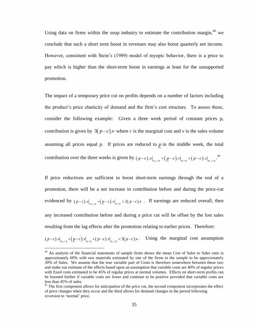
Using data on firms within the soup industry to estimate the contribution margin,40

we

conclude that such a short term boost in revenues may also boost quarterly net income.

However, consistent with Stein‟s (1989) model of myopic behavior, there is a price to

pay which is higher than the short-term boost in earnings at least for the unsupported

promotion.

The impact of a temporary price cut on profits depends on a number of factors including

the product‟s price elasticity of demand and the firm‟s cost structure. To assess these,

consider the following example: Given a three week period of constant prices p,

contribution is given by 3 .p c v where c is the marginal cost and v is the sales volume

assuming all prices equal p. If prices are reduced to p in the middle week, the total

contribution over the three weeks is given by 1 1

. . .t t tp p p p p p

p c v p c v p c v

.41

If price reductions are sufficient to boost short-term earnings through the end of a

promotion, there will be a net increase in contribution before and during the price-cut

evidenced by 1

. . 2 .t tp p p p

p c v p c v p c v

. If earnings are reduced overall, then

any increased contribution before and during a price cut will be offset by the lost sales

resulting from the lag effects after the promotion relating to earlier prices. Therefore:

1 1

. . . 3 .t t tp p p p p p

p c v p c v p c v p c v

. Using the marginal cost assumption

40

An analysis of the financial statements of sample firms shows the mean Cost of Sales to Sales ratio is

approximately 60% with raw materials estimated by one of the firms in the sample to be approximately

30% of Sales. We assume that the true variable part of Costs is therefore somewhere between these two

and make our estimate of the effects based upon an assumption that variable costs are 40% of regular prices

with fixed costs estimated to be 45% of regular prices at normal volumes. Effects on short-term profits can

be boosted further if variable costs are lower and continue to be positive provided that variable costs are

less than 45% of sales. 41

The first component allows for anticipation of the price cut, the second component incorporates the effect

of price changes when they occur and the third allows for demand changes in the period following

reversion to „normal‟ price.

36

mentioned above,42

the regression model estimates presented in the previous section

imply that a one week, one-third off price reduction would result in an increase in

quarterly revenues of approximately 11% and quarterly EPS of 5.5% through the end of

the promotion. Different effects on EPS may be achieved by discounting prices further

depending on the operating and financial leverage of the firm. However, the presence of

the post-promotion dip associated with the lag effects after of earlier prices means that

the one-week one-third off price promotion will be costly overall. In this case, the

overall effect of boosting this quarter‟s figures equates to a cost in the following period of

approximately 7.5% of quarterly net income suggesting that unsupported promotions

will, on average, be costly overall to the firm. In contrast, using the increases in sales

volumes associated with supported promotions, it is feasible that the boost in earnings for

supported promotions exceeds the cost of running the support.

Before concluding that the promotions observed in our data are negative overall to the

promoting firms, however, we must also consider the possibility of long-term benefits in

terms of customer retention and/or buying patterns.43

In this regard, the overwhelming

evidence presented in prior Marketing literature is clear; at best, sales promotions have no

long-term positive impact either on consumer behavior or on sales;44

at worst, sales

promotions lead to some negative long-term consequences.45

Such longer term effects

might be considered comparable to the sacrifice of future profits associated with earnings

management related reductions in research and development expenditure.

42

Variable costs are assumed to be 40% of regular prices with fixed costs estimated to be 45% of regular

prices at normal volumes. Higher variable cost assumptions result in lower estimates of increased earnings

associated with price cuts and greater cost of promotion overall. 43

We thank the anonymous referee for raising this possibility. 44

See Pauwels, Hanssens and Siddarth (2002) 45

See Mela, Gupta and Lehman (1997), Mela, Jedidi and Bowman (1998), Jedidi, Mela and Gupta (1999)

or Kopalle, Mela and Marsh (1999) for examples.

37

In particular, Mela, Gupta and Lehmann (1997) find that when compared to the “good”

effects of advertising, promotions have significantly larger “bad” effects on consumers‟

price and promotion sensitivities. They show that price promotions make both loyal and

non-loyal consumers more price-sensitive and train consumers to look for deals in the

marketplace. Similarly, Mela, Jedidi and Bowman (1998) show that promotions teach

consumers to “lie in wait” for especially good deals so that they can stockpile goods.

Finally, Kopalle, Mela and Marsh (1999) show that promotions can lead to a “triple

jeopardy” in which: (1) baseline sales decrease as discounts become more endemic, (2)

consumers become more price sensitive, making it more difficult to command higher

margins, and (3) deals become a less effective tool for “stealing” sales from competing

brands when they are frequently used.

These consensus results raise the question as to why firms may permit managers to run

value-destroying promotions. Several hypotheses are possible. It may be beneficial in

the short-run given the asymmetric response of stock prices to earnings which just beat or

missed certain earnings targets. Current shareholders may seek to increase current value

at the expense of future generations of shareholders.46

Alternatively, as discussed by

Arya, Glover and Sunder (1998), it may not be cost-effective to prevent or fully

understand the real earnings management behavior.

Overall, this evidence permits us to conclude the effects of increased promotions in our

sample, especially the unsupported ones, have a negative effect on the firms concerned.

46

See Skinner and Sloan (2002) or Brown and Caylor (2005) for further discussion of the asymmetry or

Dye (1988) for a discussion of a model of overlapping generations.

38

5. Conclusion

We have shown that the timing of marketing actions (price, feature and display

promotions) observed at the retail level is closely related to the fiscal calendar of product

manufacturers. In contrast to prior literature that suggests firms reduce discretionary

expenditures in order to boost reported earnings, we show that soup manufacturers

roughly double the frequency of all marketing promotions at the fiscal year-end and when

earnings management incentives are stronger. Further, this increase is focused more

heavily on less attractive, unsupported price promotions.

Our results imply that an important distinction needs to be made among different types of

marketing expenditures. Television advertising, which has been the focus of prior work,

produces long-run effects. We might expect firms to reduce this type of discretionary

expense prior to reporting deadlines because much of its benefit would be realized after

the deadline has passed; prior literature shows this does happen.47

Conversely, price,

feature and display promotions, which are the focus of our study, produce short-run

effects. Firms might be expected to invest more in these types of actions prior to

reporting deadlines, and we show that this also does happen.

Our study also provides observational evidence in support of previous survey work that

suggests managers are willing to sacrifice long-term value in order to smooth earnings

and prefer to use real actions over accounting actions to meet earnings benchmarks

(Graham, Harvey and Rajgopal, 2005). We estimate that soup manufacturers use price

reductions to legally boost sales revenues and quarterly earnings by almost 5% at the

47

See for example Mizik and Jacobson, (2007).

39

fiscal year-end. Nevertheless, there is a price to pay, as we estimate that quarterly EPS

falls by almost 7.5% in the subsequent reporting period, resulting in a net loss of 2.5% of

quarterly EPS to the manufacturer.

Finally, we show that firms systematically alter their pricing and promotion strategies

both within and across brands when incentive to manage earnings upwards are stronger.

Within brands, we show that firms make deeper price reductions for higher revenue

UPCs following periods of poor financial performance. More interestingly, across brands

we find that firms shift display promotions away from smaller revenue brands and

towards larger ones following periods of poor financial performance. This is consistent

with the actions being directed, at least in part, by parties higher in the organization than

the brand managers, as no individual brand manager would voluntarily give up aisle

displays in support for his or her brand. Together, these results imply that firms make

systematic decisions across their product lines to manage earnings.

Our results will be of interest to practitioners negotiating with suppliers as well as those

responsible for setting price and promotion strategy in response to competitor actions; we

show that a firm‟s internal desire to meet or beat earnings benchmarks can help determine

when it will take marketing actions. The final results relating to the level of those

responsible for the actions may also be of interest to those designing incentive-based

compensation as well as regulators monitoring reporting of fiscal period-ending

promotion.

40

Variable Definitions

Display is a dummy variable which equals one if there is any display promotion for the product

within the store at the time of the sale, zero otherwise.

Feature is a dummy variable which equals one if the sale is associated with a feature promotion,

zero otherwise.

HiRevBM or HighRevBrand/Manu is a dummy variable which equals one if the brand is one of

the larger revenue generating brands within the owning group.

HiRevUB or HighRevUPC/Brand is a dummy variable which equals one if the UPC is one of the

larger revenue generating UPC codes within the Brand.

Inventory Change is the change in firm level inventory over the previous 12 months

1 5 5

1 5 5

t t t

t t t

Inventory Inventory Inventory

Sales Sales Sales

JustAbove is a dummy variable which equals one if EPS for the current quarter is 100-120% of

the EPS for the same quarter in the previous year, zero otherwise.

JustBeat is a dummy variable which equals one if the manufacturer reports (ex-post) earnings for

the quarter which are between zero and 10% above the mean analyst forecast at the beginning of

the quarter and zero otherwise

JustBelow is a dummy variable which equals one if EPS for the current quarter is 80-100% of the

EPS for the same quarter in the previous year, zero otherwise.

MaxPrice is the maximum price at which the product is sold in the store over the sample period.

MissedPriorQEPS is a dummy variable which equals one if EPS for the previous quarter was 80-

100% of the EPS for the same quarter in the previous year, zero otherwise.

Pricet is the average price of the product being sold in the store during month t.

Price Change is the mean price change (in %) for the product over the previous month.

QuarterEnd is a dummy variable which equals one if the sale is during the last month of the

manufacturer‟s fiscal quarter, zero otherwise.

Special Price is a dummy variable which equals one if the sale is associated with a special price,

zero otherwise.

Weekly Units Sold is defined as the number of units of product sold at a store in a week

YearEnd is a dummy variable which equals one if the sale is during the last month of the

manufacturer‟s fiscal year, zero otherwise.

Bibliography

Aaker, David A. Managing Brand Equity. New York: The Free Press, 1991.

Arya, Anil, Jonathan Glover, and Shyam Sunder. “Earnings Management and the

Revelation Principle.” Review of Accounting Studies 3 no. 1-2 (1998): 7-34.

Bartov, E., D. Givoly, and C. Hayn. “The rewards to meeting or beating earnings

expectations.” Journal of Accounting and Economics 33 (2002): 173-204.

Blattberg, Robert C. and Scott Neslin. “Sales Promotion: Concepts, Methods, and

Strategies.” Englewood, NJ: Prentice Hall, 1990

Brown, Lawrence D. and Marcus L. Caylor. “A Temporal Analysis of Quarterly Earnings

Thresholds: Propensities and Valuation Consequences.” The Accounting Review

80 no. 2 (2005): 423-440.

Burgstahler, David and Ilia Dichev. “Earnings Management to Avoid Earnings Decreases

and Losses.” Journal of Accounting and Economics 24 no. 1 (1997): 99-126.

Bushee, Brian J. “The Influence of Institutional Investors on Myopic R&D Investment

Behavior.” Accounting Review 73 no. 3 (1998): 305-333.

Campbell Soup Company, 19 May 2008, “Q3 Results Conference Call,” retrieved August

12, 2008, from

http://www.shareholder.com/visitors/event/build2/mediapresentation.cfm?compan

yid=CPB&mediaid=3148mediauserid5&=3186908&TID=385240743:82B35FE2

F9E43D27CE1A6FC92DC1AC52&popupcheck=0&shexp=200808121225&shke

y=9710057300dc3836655445c61c879d42&player=1. Also available at

http://seekingalpha.com/article/77913-campbell-soup-f3q08-qtr-end-4-27-08-

earnings-call-transcript?page=-1

42

Chapman, Craig J. “The Effects of Real Earnings Management on the Firm, Its Competitors and

Subsequent Reporting Periods.” Northwestern University, Working Paper (2010).

Cheng, Shijun. “R&D Expenditures and CEO Compensation.” The Accounting Review 79

no. 2 (2004): 305-328.

Cohen, Daniel A., Raj Mashruwala, and Tzachi Zach. "The Use of Advertising Activities

to Meet Earnings Benchmarks: Evidence from Monthly Data." Review of

Accounting Studies, Forthcoming (2009).

Dechow, Patricia M. and Richard G. Sloan. “Executive Incentives and the Horizon

Problem.” Journal of Accounting and Economics 14 no. 1 (1991): 51-89.

Durtschi, Cindy and Peter Easton. “Earnings Management? Shapes of the Frequency

Distributions of Earnings Metrics are not Evidence Ipso Facto.” Journal of

Accounting Research 43 no. 4 (2005): 557-592.

Dye, Ronald A., “Earnings Management in an Overlapping Generations Model.” Journal

of Accounting Research 26(2) (1988): 195-235.

Fudenberg, Drew and Jean Tirole. “A Theory of Income and Dividend Smoothing Based

on Incumbency Rents.” Journal of Political Economy 103 no. 1 (1995): 75-93.

Graham, John R., Campbell R. Harvey, and Shiva Rajgopal. “The Economic Implications

of Corporate Financial Reporting.” The Journal of Accounting and Economics 40

no. 1-3 (2005): 3-73.

Gupta, Sunil. “Impact of Sales Promotions on When, What, and How Much to Buy.”

Journal of Marketing Research 25 no. 4 (1988): 342-355.

Hagle, Timothy M. and Glenn E. Mitchell. “Goodness-of-Fit Measures for Probit and

Logit.” Applied Journal of Political Science 36 no. 3 (2001): 762-784.

43

Hanssens, Dominique M., Koen Pauwels, and S. Siddarth. “The Long-Term Effects of

Price Promotions on Category Incidence, Brand Choice and Purchase Quantity.”

Journal of Marketing Research 39 no. 4 (2002): 421-439.

Hayn, Carla. “The Information Content of Losses.” Journal of Accounting & Economics

20 no. 2 (1995): 125-153.

Healy, Paul M. “The Effect of Bonus Schemes on Accounting Decisions.” Journal of

Accounting and Economics 7 no. 1-3 (1985): 85-107.

Jedidi, Kamel, Carl F. Mela and Sunil Gupta. “Managing Advertising and Promotion for

Long-Run Profitability.” Marketing Science 18 no. 1 (1999): 1-22

___ and James M. Wahlen. “A Review of the Earnings Management Literature and its

Implications for Standard Setting.” Accounting Horizons 13 no. 4 (1999): 365-

383.

Kopalle, Praveen, Carl F. Mela and Lawrence Marsh. “The Dynamic Effect of

Discounting on Sales: Empirical Analysis and Normative Pricing Inplications.”

Marketing Science 18 no. 3 (1999): 317-332

Jones, Jennifer J. “Earnings Management During Import Relief Investigations.” Journal

of Accounting Research 29 no. 2 (1991): 193-228.

Macé, Sandrine and Scott A. Neslin. “The Determinants of Pre- and Post-Promotion Dips

in Sales of Frequently Purchased Goods.” Journal of Marketing Research 41 no. 3

(2004): 339-350.

McNichols, Maureen F. “Research Design in Earnings Management Studies.” Journal of

Accounting and Public Policy 19 no. 4-5 (2000): 313-345.

44

Mela, Carl, Sunil Gupa and Donald R. Lehmann. “The Long-Term Impact of Promotion

and Advertising on Consumer Brand Choice.” Journal of Marketing Research 34

(1997): 248-261

___ , Kamel Jedidi and Douglas Bowman. “The Long-Term Impact of Promotions on

Consumer Stockpiling Behavior.” Journal of Marketing Research 35 (1998): 250-

262

Mizik, Natalie and Robert Jacobson. “Myopic Marketing Management: Evidence of the

Phenomenon and Its Long-term Performance Consequences in the SEO Context.”

Marketing Science 26 no. 3 (2007): 361-379.

Narasimhan, Chakravarthi, Scott A. Neslin, and Subrata K. Sen. “Promotional Elasticities

and Category Characteristics.” Journal of Marketing 60 no. 2 (1996): 17-30.

Oberholzer-Gee, Felix and Julie Wulf. “Earnings Management from the Bottom Up: An

Analysis of Division Manager Incentives.” 2006 Working Paper.

http://www.scholar.google.com.

Oyer, Paul. “Fiscal Year-Ends and Non-Linear Incentive Contracts: The Effect of

Business Seasonality.” Quarterly Journal of Economics 113 no. 1 (1998): 149-

185.

Roychowdhury, Sugata. “Earnings Management Through Real Activities Manipulation.”

Journal of Accounting and Economics 42 no. 3 (2006): 335-370.

Skinner, Douglas J. and Richard G. Sloan “Earnings Surprises, Growth Expectations, and

Stock Returns or Don't Let an Earnings Torpedo Sink Your Portfolio.” Review of

Accounting Studies 7 no. 2-3 (2002): 1380-6653.

Steenburgh, Thomas J. “Measuring Consumer and Competitive Impact with Elasticity

Decompositions.” Journal of Marketing Research 44 no. 4 (2007): 636-646.

45

Stein, Jeremy C. “Efficient Capital Markets, Inefficient Firms: A Model of Myopic

Corporate Behavior.” The Quarterly Journal of Economics 104 no. 4 (1989): 655-

669.

Stock, James H. and Mark W. Watson. Introduction to Econometrics. Boston, MA:

Pearson/Addison Wesley, 2007.

van Heerde, Harald J., Peter S. H. Leeflang, and Dick R. Wittink. “The Estimation of

Pre- and Post-Promotion Dips with Store-Level Scanner Data.” Journal of

Marketing Research 37 no. 3 (2000): 383-395.

___. “Decomposing the Sales Promotion Bump with Store Data.” Marketing Science 23

no. 3 (2004): 317-334.

46

Figure 1: Sales Frequency by Week in the Sample.

Week one is the beginning of the calendar year.

Figure 2: Fiscal Year-End Frequency Distribution for Companies in Sample

47

Figure 3: Frequency of Display Promotions around the Year-end

Figure 3.1 Figure 3.2

Figure 3.3 Figure 3.4

0%

1%

2%

3%

4%

5%

-2 -1 0 1 2

Frequency of Display Promotion for a Typical Year End(UPCs Within Brand)

Small UPC in Brand Large UPC in Brand

0%

1%

2%

3%

4%

5%

-2 -1 0 1 2

Frequency of Display Promotion Following Poor EPS (UPCs Within Brand)

Small UPC in Brand Large UPC in Brand

0%

1%

2%

3%

4%

5%

-2 -1 0 1 2

Frequency of Display Promotion for a Typical Year End (Brands Within Company)

Small Brand in Company Large Brand in Company

0%

1%

2%

3%

4%

5%

-2 -1 0 1 2

Frequency of Display Promotion Following Poor EPS (Brands Within Company)

Small Brand in Company Large Brand in Company

48

Figure 4: The Effect of a 20% Price Reduction on Volume and Revenues

0

0.5

1

1.5

2

2.5

Effect of a 20% Price Reduction on Volume and Revenues

Volume Revenue

We

ekly

Vo

lum

e/R

eve

nu

e in

Un

its S

tan

da

rdiz

ed t

o O

ne

for

a R

egu

lar

We

ek

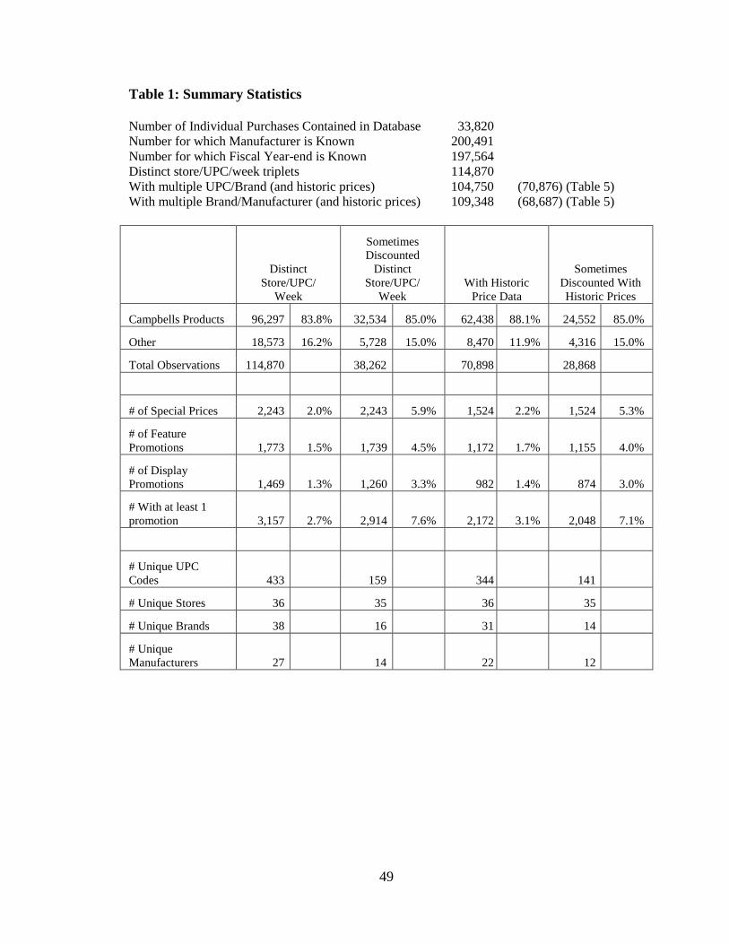
49

Table 1: Summary Statistics

Number of Individual Purchases Contained in Database 33,820

Number for which Manufacturer is Known 200,491

Number for which Fiscal Year-end is Known 197,564

Distinct store/UPC/week triplets 114,870

With multiple UPC/Brand (and historic prices) 104,750 (70,876) (Table 5)

With multiple Brand/Manufacturer (and historic prices) 109,348 (68,687) (Table 5)

Distinct

Store/UPC/

Week

Sometimes

Discounted

Distinct

Store/UPC/

Week

With Historic

Price Data

Sometimes

Discounted With

Historic Prices

Campbells Products 96,297 83.8% 32,534 85.0% 62,438 88.1% 24,552 85.0%

Other 18,573 16.2% 5,728 15.0% 8,470 11.9% 4,316 15.0%

Total Observations 114,870 38,262 70,898 28,868

# of Special Prices 2,243 2.0% 2,243 5.9% 1,524 2.2% 1,524 5.3%

# of Feature

Promotions 1,773 1.5% 1,739

4.5% 1,172 1.7% 1,155 4.0%

# of Display

Promotions 1,469 1.3% 1,260

3.3% 982 1.4% 874 3.0%

# With at least 1

promotion 3,157 2.7% 2,914

7.6% 2,172 3.1% 2,048 7.1%

# Unique UPC

Codes 433

159

344 141

# Unique Stores 36 35 36 35

# Unique Brands 38 16 31 14

# Unique

Manufacturers 27

14

22 12

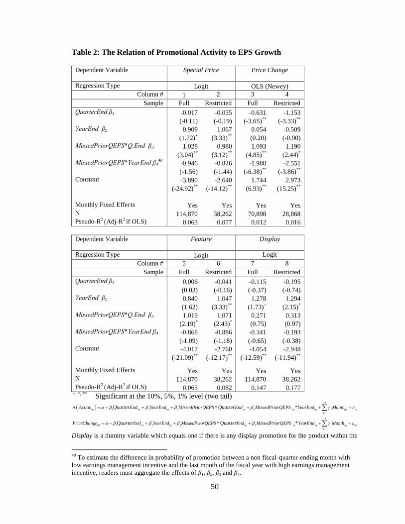
50

Table 2: The Relation of Promotional Activity to EPS Growth

Dependent Variable

Special Price

Price Change

Regression Type Logit OLS (Newey)

Column # 1 2 3 4

Sample Full Restricted Full Restricted

QuarterEnd β1 -0.017 -0.035 -0.631 -1.153

(-0.11) (-0.19) (-3.65)**

(-3.33)**

YearEnd β2 0.909 1.067 0.054 -0.509

(1.72)+ (3.33)

** (0.20) (-0.90)

MissedPriorQEPS*Q.End β3 1.028 0.980 1.093 1.190

(3.04)**

(3.12)**

(4.85)**

(2.44)*

MissedPriorQEPS*YearEnd β448

-0.946 -0.826 -1.988 -2.551

(-1.56) (-1.44) (-6.38)**

(-3.86)**

Constant -3.890 -2.640 1.744 2.973

(-24.92)**

(-14.12)**

(6.93)**

(15.25)**

Monthly Fixed Effects Yes Yes Yes Yes

N 114,870 38,262 70,898 28,868

Pseudo-R2 (Adj-R

2 if OLS) 0.063 0.077 0.012 0.016

Dependent Variable

Feature

Display

Regression Type Logit Logit

Column # 5 6 7 8

Sample Full Restricted Full Restricted

QuarterEnd β1 0.006 -0.041 -0.115 -0.195

(0.03) (-0.16) (-0.37) (-0.74)

YearEnd β2 0.840 1.047 1.278 1.294

(1.62) (3.33)**

(1.73)+ (2.15)

*

MissedPriorQEPS*Q.End β3 1.019 1.071 0.271 0.313

(2.19)* (2.43)

* (0.75) (0.97)

MissedPriorQEPS*YearEnd β4 -0.868 -0.886 -0.341 -0.193

(-1.09) (-1.18) (-0.65) (-0.38)

Constant -4.017 -2.760 -4.054 -2.948

(-21.09)**

(-12.17)**

(-12.59)**

(-11.94)**

Monthly Fixed Effects Yes Yes Yes Yes

N 114,870 38,262 114,870 38,262

Pseudo-R2 (Adj-R

2 if OLS) 0.065 0.082 0.147 0.177

+, *, ** Significant at the 10%, 5%, 1% level (two tail)

12

1 2 3 4

1

*ist ist ist ist ist ist j istj ist

j

Action End YearEnd MissedPriorQEPS * End MissedPriorQEPS YearEnd MonthQuarter Quarter

12

1 2 3 4

1

*ist ist ist ist ist j istj ist

j

istPriceChange End YearEnd MissedPriorQEPS * End MissedPriorQEPS YearEnd MonthQuarter Quarter

Display is a dummy variable which equals one if there is any display promotion for the product within the

48

To estimate the difference in probability of promotion between a non fiscal-quarter-ending month with

low earnings management incentive and the last month of the fiscal year with high earnings management

incentive, readers must aggregate the effects of β1, β2, β3 and β4.

51

store at the time of the sale, zero otherwise. Feature is a dummy variable which equals one if the sale is

associated with a feature promotion, zero otherwise. MissedPriorQEPS is a dummy variable which equals

one if EPS for the previous quarter was 80-100% of the EPS for the same quarter in the previous year, zero

otherwise. Price Change is the mean price change (in %) for the product over the previous month.

QuarterEnd is a dummy variable which equals one if the sale is during the last month of the manufacturer‟s

fiscal quarter, zero otherwise. Special Price is a dummy variable which equals one if the sale is associated

with a special price, zero otherwise. YearEnd is a dummy variable which equals one if the sale is during

the last month of the manufacturer‟s fiscal year, zero otherwise.

52

Table 3: The Relation of Promotional Activity to Analyst Forecasts

Dependent Variable

Special Price

Price Change

Regression Type Logit OLS (Newey)

Column # 1 2 3 4

Sample Full Restricted Full Restricted

QuarterEnd β1 0.134 0.138 -0.772 -1.641

(0.38) (0.38) (-5.24)**

(-5.45)**

JustBeat β2 -0.896 -0.967 0.332 0.609

(-3.96)**

(-4.87)**

(4.18)**

(3.35)**

JustBeat*QuarterEnd β3 1.186 1.208 0.287 0.290

(4.99)**

(5.03)**

(1.81)+ (0.81)

Constant -4.031 -2.791 0.571 -1.593

(-14.18)**

(-8.46)**

(3.16)**

(-8.01)**

Monthly Fixed Effects Yes Yes Yes Yes

N

112,247 37,136 69,775 28,221

Pseudo-R2 (Adj-R

2 if OLS) 0.088 0.104 0.0138 0.0198

Dependent Variable

Feature

Display

Regression Type Logit OLS (Newey)

Column # 5 6 7 8

Sample Full Restricted Full Restricted

QuarterEnd β1 0.183 0.170 0.158 0.035

(0.52) (0.43) (1.75)+ (0.27)

JustBeat β2 -0.759 -0.818 -0.440 -0.503

(-3.77)**

(-4.82)**

(-1.48) (-1.80)+

JustBeat*QuarterEnd β3 1.044 1.066 0.638 0.702

(4.16)**

(4.12)**

(2.32)* (2.38)

*

Constant -4.173 -2.935 -4.283 -3.122

(-13.60)**

(-8.30)**

(-21.92)**

(-20.07)**

Monthly Fixed Effects Yes Yes Yes Yes

N 112,247 37,136 112,247 37,136

Pseudo-R2 0.075 0.091 0.147 0.179

+, *, ** Significant at the 10%, 5%, 1% level (two tail)

Display is a dummy variable which equals one if there is any display promotion for the product within the

store at the time of the sale, zero otherwise. Feature is a dummy variable which equals one if the sale is

associated with a feature promotion, zero otherwise. JustBeat is a dummy variable which equals one if the

manufacturer reports (ex-post) earnings for the quarter are between zero and 10% above the consensus

analyst forecast at the beginning of the quarter and zero otherwise. Price Change is the mean price change

(in %) for the product over the previous month. QuarterEnd is a dummy variable which equals one if the

sale is during the last month of the manufacturer‟s fiscal quarter, zero otherwise. Special Price is a dummy

variable which equals one if the sale is associated with a special price, zero otherwise.

53

Table 4: The Relation of Promotional Support to EPS Growth

Dependent Variable

Special Price

Regression Type Logit

Column # 1 2

Sample Full Restricted

QuarterEnd β1 0.035 0.167

(0.18) (0.83)

YearEnd β2 -0.003 0.054

(-0.01) (0.18)

MissedPriorQEPS*Q.End β3 0.769 0.587

(2.79)**

(3.05)**

MissedPriorQEPS*YearEnd β449

-0.815 -0.599

(-2.22)* (-1.57)

Feature β5 5.380 4.552

(22.17)**

(23.70)**

Display β6 7.901 6.914

(17.53)**

(16.17)**

Constant -6.413 -5.278

(-27.08)**

(-20.41)**

Monthly Fixed Effects Yes Yes

N

114,870 38,262

Pseudo-R2 (Adj-R

2 if OLS) 0.346 0.510

+, *, ** Significant at the 10%, 5%, 1% level (two tail)

Display is a dummy variable which equals one if there is any display promotion for the product within the

store at the time of the sale, zero otherwise. Feature is a dummy variable which equals one if the sale is

associated with a feature promotion, zero otherwise. MissedPriorQEPS is a dummy variable which equals

one if EPS for the previous quarter was 80-100% of the EPS for the same quarter in the previous year, zero

otherwise. QuarterEnd is a dummy variable which equals one if the sale is during the last month of the

manufacturer‟s fiscal quarter, zero otherwise. Special Price is a dummy variable which equals one if the

sale is associated with a special price, zero otherwise. YearEnd is a dummy variable which equals one if

the sale is during the last month of the manufacturer‟s fiscal year, zero otherwise.

49

To estimate the difference in probability of promotion between a non fiscal-quarter-ending month with

low earnings management incentive and the last month of the fiscal year with high earnings management

incentive, readers must aggregate the effects of β1, β2, β3 and β4.

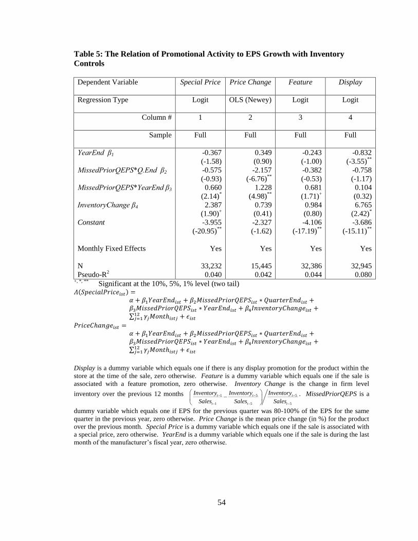
54

Table 5: The Relation of Promotional Activity to EPS Growth with Inventory

Controls

Dependent Variable

Special Price Price Change Feature Display

Regression Type

Logit OLS (Newey) Logit Logit

Column # 1

2 3 4

Sample

Full Full Full Full

YearEnd β1 -0.367 0.349 -0.243 -0.832

(-1.58) (0.90) (-1.00) (-3.55)**

MissedPriorQEPS*Q.End β2 -0.575 -2.157 -0.382 -0.758

(-0.93) (-6.76)**

(-0.53) (-1.17)

MissedPriorQEPS*YearEnd β3 0.660 1.228 0.681 0.104

(2.14)* (4.98)

** (1.71)

+ (0.32)

InventoryChange β4 2.387 0.739 0.984 6.765

(1.90)+ (0.41) (0.80) (2.42)

*

Constant -3.955 -2.327 -4.106 -3.686

(-20.95)**

(-1.62) (-17.19)**

(-15.11)**

Monthly Fixed Effects Yes Yes Yes Yes

N 33,232 15,445 32,386 32,945

Pseudo-R2 0.040 0.042 0.044 0.080

+, *, ** Significant at the 10%, 5%, 1% level (two tail)

Display is a dummy variable which equals one if there is any display promotion for the product within the

store at the time of the sale, zero otherwise. Feature is a dummy variable which equals one if the sale is

associated with a feature promotion, zero otherwise. Inventory Change is the change in firm level

inventory over the previous 12 months 1 5 5

1 5 5

t t t

t t t

Inventory Inventory Inventory

Sales Sales Sales

. MissedPriorQEPS is a

dummy variable which equals one if EPS for the previous quarter was 80-100% of the EPS for the same

quarter in the previous year, zero otherwise. Price Change is the mean price change (in %) for the product

over the previous month. Special Price is a dummy variable which equals one if the sale is associated with

a special price, zero otherwise. YearEnd is a dummy variable which equals one if the sale is during the last

month of the manufacturer‟s fiscal year, zero otherwise.

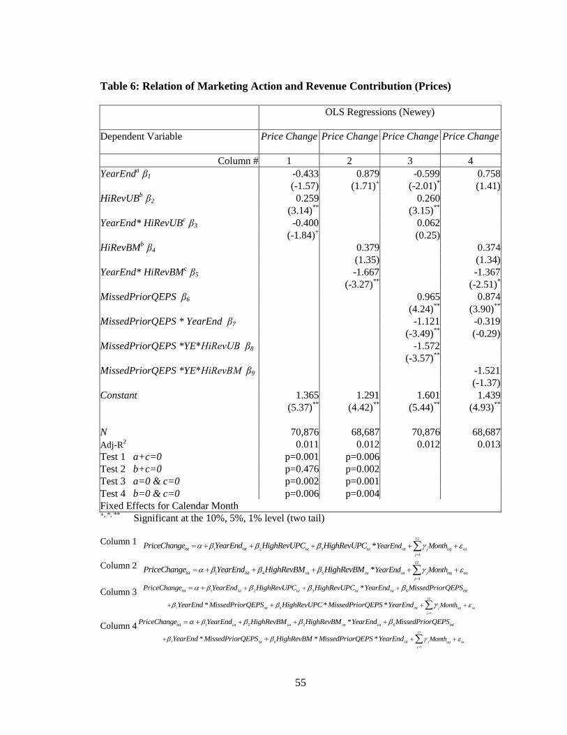
55

Table 6: Relation of Marketing Action and Revenue Contribution (Prices)

OLS Regressions (Newey)

Dependent Variable

Price Change Price Change Price Change Price Change

Column # 1 2 3 4

YearEnda

β1 -0.433 0.879 -0.599 0.758

(-1.57) (1.71)+ (-2.01)

* (1.41)

HiRevUBb

β2 0.259 0.260

(3.14)**

(3.15)**

YearEnd* HiRevUBc

β3 -0.400 0.062

(-1.84)+ (0.25)

HiRevBMb

β4 0.379 0.374

(1.35) (1.34)

YearEnd* HiRevBMc

β5 -1.667 -1.367

(-3.27)**

(-2.51)*

MissedPriorQEPS β6 0.965 0.874

(4.24)**

(3.90)**

MissedPriorQEPS * YearEnd β7 -1.121 -0.319

(-3.49)**

(-0.29)

MissedPriorQEPS *YE*HiRevUB β8 -1.572

(-3.57)**

MissedPriorQEPS *YE*HiRevBM β9 -1.521

(-1.37)

Constant 1.365 1.291 1.601 1.439

(5.37)**

(4.42)**

(5.44)**

(4.93)**

N 70,876 68,687 70,876 68,687

Adj-R2 0.011 0.012 0.012 0.013

Test 1 a+c=0 p=0.001 p=0.006

Test 2 b+c=0 p=0.476 p=0.002

Test 3 a=0 & c=0 p=0.002 p=0.001

Test 4 b=0 & c=0 p=0.006 p=0.004

Fixed Effects for Calendar Month +, *, **

Significant at the 10%, 5%, 1% level (two tail)

Column 1 12

1 2 3

1

*ist ist ist j istj ist

j

ist ist YearEnd MonthPriceChange YearEnd HighRevUPC HighRevUPC

Column 2 12

1 4 5

1

*ist ist ist j istj ist

j

ist ist YearEnd MonthPriceChange YearEnd HighRevBM HighRevBM

Column 3 12

7 8

1

1 2 3 6*

* * *j istj ist

j

ist ist ist ist

ist ist

ist ist

Month

PriceChange YearEnd HighRevUPC HighRevUPC YearEnd MissedPriorQEPS

YearEnd MissedPriorQEPS HighRevUPC MissedPriorQEPS YearEnd

Column 412

7 8

1

1 2 3 6*

* * *j istj ist

j

ist ist ist ist

ist ist

ist ist

Month

PriceChange YearEnd HighRevBM HighRevBM YearEnd MissedPriorQEPS

YearEnd MissedPriorQEPS HighRevBM MissedPriorQEPS YearEnd

56

HiRevBM is a dummy variable which equals one if the brand is one of the larger revenue generating brands

within the owning group. HiRevUB is a dummy variable which equals one if the UPC is one of the larger

revenue generating UPC codes within the Brand.MissedPriorQEPS is a dummy variable which equals one

if EPS for the previous quarter was 80-100% of the EPS for the same quarter in the previous year, zero

otherwise. Price Change is the mean price change (in %) for the product over the previous month.

YearEnd (YE) is a dummy variable which equals one if the sale is during the last month of the

manufacturer‟s fiscal year, zero otherwise.

57

Table 7: Relation of Marketing Action and Revenue Contribution (Display)

Logistic Regressions

Dependent Variable

Display Display

Display

Display

Column # 1 2 3 4

YearEnda

β1 1.064 1.259 1.183 1.329

(2.93)**

(3.60)**

(3.18)**

(4.01)**

HiRevUBb

β2 1.337 1.338

(5.49)**

(5.51)**

YearEnd*HiRevUBc

β3 -0.369 -0.512

(-0.98) (-1.25)

HiRevBMb

β4 -0.618 -0.620

(-1.72)+ (-1.73)

+

YearEnd*HiRevBMc

β5 -0.038 -0.107

(-0.07) (-0.19)

MissedPriorQEPS β6 0.349 0.265

(0.95) (0.71)

MissedPriorQEPS*YE β7 -0.961 -1.145

(-1.07) (-1.86)+

MissedPriorQEPS*YE*HiRevUB β8 0.794

(0.98)

MissedPriorQEPS *YE*HiRevBM β9 0.869

(1.83)+

Constant -4.810 -3.556 -4.811 -3.554

(-23.24)**

(-11.58)**

(-23.26)**

(-11.59)**

N 104,750 109,348 104,750 109,348

Pseudo- R2 0.074 0.152 0.074 0.152

Test 1 a+c=0 p=0.134 p=0.053

Test 2 b+c=0 p=0.015 p=0.015

Test 3 a=0 & c=0 p=0.013 p=0.226

Test 4 b=0 & c=0 p=0.000 p=0.188

Fixed Effects for Calendar Month +, *, **

Significant at the 10%, 5%, 1% level (two tail)

Column 1 12

1 2 3

1

*ist ist ist j istj ist

j

ist ist YearEnd MonthDisplay YearEnd HighRevUPC HighRevUPC

Column 2 12

1 4 5

1

*ist ist ist j istj ist

j

ist ist YearEnd MonthDisplay YearEnd HighRevBM HighRevBM

Column 3 12

7 8

1

1 2 3 6*

* * *j istj ist

j

ist ist ist ist

ist ist

ist ist

Month

YearEnd HighRevUPC HighRevUPC YearEnd MissedPriorQEPS

YearEnd MissedPriorQEPS HighRevUPC MissedPriorQEPS YearEnd

Display

Column 4 12

7 9

1

1 4 5 6*

* * *j istj ist

j

ist ist ist ist

ist ist

ist ist

Month

YearEnd HighRevBM HighRevBM YearEnd MissedPriorQEPS

YearEnd MissedPriorQEPS HighRevBM MissedPriorQEPS YearEnd

Display

Display is a dummy variable which equals one if there is any display promotion for the product within the

store at the time of the sale, zero otherwise. HiRevBM is a dummy variable which equals one if the brand is

one of the larger revenue generating brands within the owning group. HiRevUB is a dummy variable which

equals one if the UPC is one of the larger revenue generating UPC codes within the

Brand.MissedPriorQEPS is a dummy variable which equals one if EPS for the previous quarter was 80-

58

100% of the EPS for the same quarter in the previous year, zero otherwise. YearEnd (YE) is a dummy

variable which equals one if the sale is during the last month of the manufacturer‟s fiscal year, zero

otherwise.

59

Table 8: Impact of Marketing Actions on the Timing of Consumers’ Purchases

Dependent Variable

Ln(Weekly Units Sold)

Regression Type

OLS (Newey)

Column # 1 2

Ln(Pricet-1/MaxPrice) β1 0.606 0.423

(3.00)**

(2.48)*

Ln(Pricet/MaxPrice) β2 -3.378 -3.126

(-9.88)**

(-8.63)**

Ln(Pricet+1/MaxPrice) β3 1.418 1.392

(4.80)**

(4.67)**

Display β4 1.023 0.638

(7.48)**

(2.51)*

Display * Ln(Pricet/MaxPrice) β5 -0.520

(-1.92)+

Feature β6 2.070 1.454

(10.94)**

(6.81)**

Feature * Ln(Pricet/MaxPrice) β7 -0.672

(-3.18)**

Constant 6.250 6.255

(73.85)**

(73.21)**

Fixed Effects for UPC as well as Calendar Month

N 27,008 27,008

Adj-R2 0.428 0.430

+, *, ** Significant at the 10%, 5%, 1% level (two tail)

Column 1 , 1 , 1

1 2 3

12

4 6

1

Pr PrPr

Pr Pr Pr

is t is tistist

is is is

ist ist j istj i i ist

j i

ice iceiceLn WeeklyUnitsSold Ln Ln Ln

Max ice Max ice Max ice

Display Feature Month UPC

Column 2

, 1 , 1

1 2 3 4

5 6 7

Pr PrPr

Pr Pr Pr

Pr Pr* *

Pr

is t is tistist ist

is is is

istist ist ist

is

ice iceiceLn WeeklyUnitsSold Ln Ln Ln Display

Max ice Max ice Max ice

ice iDisplay Ln Feature Feature Ln

Max ice

12

1

Pr

ist

is

j istj i i ist

j i

ce

Max ice

Month UPC

Display is a dummy variable which equals one if there is any display promotion for the product within the

store at the time of the sale, zero otherwise. Feature is a dummy variable which equals one if the sale is

associated with a feature promotion, zero otherwise. MaxPrice is the maximum price at which the product

is sold in the store over the sample period. Pricet is the average price of the product being sold in the store

during month t. Weekly Units Sold is defined as the number of units of product sold at a store in a week.