Embed Size (px)
Citation preview

AN INVESTIGATION OF JAMMING TECHNIQUES THROUGH A RADAR
RECEIVER SIMULATION
A THESIS SUBMITTED TO THE GRADUATE SCHOOL OF NATURAL AND APPLIED SCIENCES
OF MIDDLE EAST TECHNICAL UNIVERSITY
BY
ATİYE ASLI KIRKPANTUR-ÇADALLI
IN PARTIAL FULFILLMENT OF THE REQUIREMENTS FOR
THE DEGREE OF MASTER OF SCIENCE IN
ELECTRICAL AND ELECTRONICS ENGINEERING
DECEMBER 2007

Approval of the thesis:
AN INVESTIGATION OF JAMMING TECHNIQUES THROUGH A RADAR RECEIVER SIMULATION
submitted by ATİYE ASLI KIRKPANTUR-ÇADALLI in partial fulfillment of the requirements for the degree of Master of Science in Electrical and Electronics Engineering Department, Middle East Technical University by, Prof. Dr. Canan Özgen _____________________ Dean, Graduate School of Natural and Applied Sciences Prof. Dr. İsmet Erkmen _____________________ Head of Department, Electrical and Electronics Engineering Assoc. Prof. Dr. Sencer Koç _____________________ Supervisor, Electrical and Electronics Engineering Dept., METU Prof. Dr. Yalçın Tanık _____________________ Co-Supervisor, Electrical and Electronics Engineering Dept., METU Examining Committee Members: Prof. Dr. Fatih Canatan _____________________ Electrical and Electronics Engineering Dept., METU Assoc. Prof. Dr. Sencer Koç _____________________ Electrical and Electronics Engineering Dept., METU Prof. Dr. Yalçın Tanık _____________________ Electrical and Electronics Engineering Dept., METU Assist. Prof. Dr. Çağatay Candan _____________________ Electrical and Electronics Engineering Dept., METU Dr. Mehmet Ali Tuğay _____________________ Engineering Director, MİKES
Date: 6 December 2007

iii
I hereby declare that all information in this document has been obtained and
presented in accordance with academic rules and ethical conduct. I also
declare that, as required by these rules and conduct, I have fully cited and
referenced all material and results that are not original to this work.
Name, Last Name : Atiye Aslı Kırkpantur-Çadallı
Signature :

iv
1.ABSTRACT
AN INVESTIGATION OF JAMMING TECHNIQUES THROUGH A RADAR
RECEIVER SIMULATION
Kırkpantur-Çadallı, Atiye Aslı
M.S., Department of Electrical and Electronics Engineering
Supervisor : Assoc. Prof. Dr. Sencer Koç
Co- Supervisor: Prof. Dr. Yalçın Tanık
December 2007, 120 pages
In this study, various jamming techniques and their effects on detection and
tracking performance have been investigated through a radar receiver simulation
that models a search radar for target acquisition and single-target tracking radar
during track operation. The radar is modeled as looking at airborne targets, and
hence clutter is not considered. Customized algorithms have been developed for the
detection of target azimuth angle, range and Doppler velocity within the modeled
geometry and chosen radar parameters. The effects of varying parameters like
jamming-to-signal ratio (JSR) and jamming signal`s Doppler shift have been
examined in the analysis of jamming effectiveness.
Keywords: Radar Receiver, Detection, Target Tracking, RGPO, Jamming
Effectiveness

v
2.ÖZ
RADAR KARIŞTIRMA YÖNTEMLERİNİN BİR RADAR ALMAÇ BENZETİMİ
ÜZERİNDE İNCELENMESİ
Kırkpantur-Çadallı, Atiye Aslı
Yüksek Lisans Tezi, Elektrik ve Elektronik Mühendisliği Bölümü
Tez Yöneticisi : Doç. Dr. Sencer Koç
Ortak Tez Yöneticisi: Prof. Dr. Yalçın Tanık
Aralık 2007, 120 sayfa
Bu çalışmada, değişik karıştırma teknikleri ile bu tekniklerin radar hedef tespit ve
izleme başarımına etkileri, hedef arama modunda tarama radarı olarak çalışan ve
hedef takip modunda, tek hedef takibi yapan bir radar almaç benzetimi üzerinde
incelenmiştir. Benzetimi yapılan radar modeli, hava hedeflerini ve hava
platformunu kapsamaktadır. Bu nedenle yüzey kargaşasının benzetimi gerekli
görülmemiştir. Model yapısı ve seçilen radar parametreleri dikkate alınarak hedefin
açısal koordinatının, menzilinin ve Doppler frekans kaymasının tespiti için uygun
algoritmalar geliştirilmiştir. Karıştırma-sinyal oranı ve karıştırma sinyalinin frekans
kayması gibi parametreler değiştirilerek karıştırma etkinliği incelenmiştir.
Anahtar Kelimeler: Radar Almacı, Tespit, Hedef İzleme, RGPO, karıştırma
etkinliği

vi
To My Parents and My Husband

vii
3.ACKNOWLEDGEMENTS
I would like to express my deepest gratitude to my supervisor Assoc. Prof. Dr.
Sencer Koç and co-supervisor Prof. Dr. Yalçın Tanık for their guidance, insightful
advice and criticism, and constant encouragement throughout this research.
I would like to thank my colleagues at MİKES Inc. for their support on every phase
of this work.
I would like to thank my whole family for their constant care and understanding
throughout my life and their sincere trust that I could accomplish this task.
I would like to thank my husband for his support and tolerance during my thesis
study.

viii
4.TABLE OF CONTENTS
ABSTRACT ........................................................................................................... iv
ÖZ ........................................................................................................................... v
ACKNOWLEDGEMENTS ................................................................................... vii
TABLE OF CONTENTS...................................................................................... viii
CHAPTER
1 1. INTRODUCTION ............................................................................................ 1
2 2. BASIC PRINCIPLES OF RADAR................................................................... 3
2.1 Classification of Radars............................................................................ 3
2.2 The Radar Equation.................................................................................. 4
2.3 Basic Pulsed Radar Block Diagram .......................................................... 4
2.3.1 Pulse-Doppler radar .......................................................................... 6
2.4 Radar Block Diagram Basic Elements ...................................................... 8
2.4.1 Synchronizer..................................................................................... 8
2.4.2 Modulator......................................................................................... 8
2.4.3 Transmitter ....................................................................................... 8
2.4.4 Duplexer........................................................................................... 8
2.4.5 Antenna ............................................................................................ 8
2.4.6 Receiver protection device ................................................................ 9
2.4.7 Receiver............................................................................................ 9
2.4.8 Indicator ..........................................................................................10
2.4.9 Antenna servo..................................................................................10
2.5 Target Tracking.......................................................................................11
2.5.1 Single target tracking (continuous tracking) .....................................11
2.5.1.1 Angle tracking .............................................................................11
2.5.1.2 Range tracking.............................................................................12
2.5.2 Multiple target tracking....................................................................13
3 3. RADAR SIMULATION..................................................................................15
3.1 Transmitter-Receiver Simulation .............................................................15

ix
3.2 Delay-Doppler Detection.........................................................................22
3.2.1 Computation of the power spectral density.......................................22
3.2.2 Detection using PSD........................................................................24
3.3 Azimuth Angle Detection ........................................................................28
3.4 Tracking ..................................................................................................30
3.4.1 Tracking Filter .................................................................................32
3.5 Tracking Performance under No Jamming...............................................37
4 4. JAMMING AND ITS EFFECTIVENESS .......................................................48
4.1 The Jamming Concept .............................................................................48
4.1.1 Noise Technique ..............................................................................48
4.1.2 Range Gate Pull Off (RGPO)...........................................................49
4.1.2.1 Jamming procedure......................................................................51
4.1.2.2 ECM parameters..........................................................................53
4.1.2.3 Required radar signal parameters .................................................53
4.1.3 Related Techniques..........................................................................54
4.1.3.1 RGPI 54
4.1.3.2 Overlapped RGPO.......................................................................55
4.1.3.3 RGPO with hold out (hook) .........................................................55
4.2 Tracking Performance under Jamming.....................................................56
4.2.1 Spot-Noise Jamming........................................................................56
4.2.2 RGPO..............................................................................................64
4.2.3 RGPI ...............................................................................................79
4.2.4 Overlapped RGPO ...........................................................................86
4.2.5 RGPO with hold-out ........................................................................92
5 5. CONCLUSIONS ...........................................................................................100
REFERENCES .....................................................................................................103

x
LIST OF FIGURES
Figure 2-1: Basic pulse radar block diagram...........................................................5
Figure 2-2: Radar receiver block diagram.............................................................10
Figure 3-1: Depiction of the simulated radar scenario............................................17
Figure 3-2: Target range within the search period..................................................19
Figure 3-3: Received power in the search period. ..................................................19
Figure 3-4: Scanning antenna pattern gain in the search period. ............................20
Figure 3-5: Received radar signal with white Gaussian noise. ...............................22
Figure 3-6: Power spectral density of the received pulses as a function of delay and
Doppler frequency. ...............................................................................................23
Figure 3-7: Projection of PSD along the Doppler axis onto the delay axis. ...........25
Figure 3-8: Magnified version of Figure 3-7. Detection threshold is indicated.......25
Figure 3-9: Doppler frequency reading from the cross section of PSD...................26
Figure 3-10: Received signal as a function of the radar scan angle is used for angle
detection. ..............................................................................................................29
Figure 3-11: Angle detection is performed using curve fitting. ..............................29
Figure 3-12: Data collection of the radar in the search and track modes.................32
Figure 3-13: Pole-zero plot of the tracking filter with ξ = 0.8...............................35
Figure 3-14: Range performance of the tracking filter; update interval is 0.05 s;
smoothing coefficient is 0.8. .................................................................................36
Figure 3-15: Velocity performance of the tracking filter; update interval is 0.05 s;
smoothing coefficient is 0.8. .................................................................................37
Figure 3-16: Received signal and thermal noise during the first snapshot. .............38
Figure 3-17: PSD of the return signal within the range gate, and its projection on
delay axis..............................................................................................................40
Figure 3-18: Doppler measurement within the first snapshot. ................................40
Figure 3-19: CFAR noise power estimate throughout the snapshots. .....................41
Figure 3-20: Range estimates/measurements for no-jamming tracking scenario. ...43
Figure 3-21: Velocity estimates/measurements for no-jamming tracking scenario. 43

xi
Figure 3-22: Error of range measurements/estimates for no-jamming tracking
scenario. ...............................................................................................................44
Figure 3-23: Error of velocity measurements/estimates for no-jamming tracking
scenario. ...............................................................................................................44
Figure 3-24: Range estimates/measurements for a stationary target at 10050 m.....45
Figure 3-25: Range estimates/measurements for a stationary target at 10075 m.....46
Figure 3-26: Velocity estimates/measurements for a target with no velocity
representation error. ..............................................................................................47
Figure 4-1: RGPO Video Programming Waveforms ............................................52
Figure 4-2: RGPO pulse generation......................................................................52
Figure 4-3: Target return and the jamming noise for the last snapshot (Snapshot
100) and the received signal throughout snapshots. Spot-noise, JSRspn = 6 dB. ......57
Figure 4-4: Target range, jammer transmit/received power. Spot-noise, JSRspn = 6
dB.........................................................................................................................57
Figure 4-5: CFAR noise power estimate throughout the snapshots. Spot-noise,
JSRspn = 6 dB. .......................................................................................................58
Figure 4-6: PSD for the last snapshot of spot-noise jamming simulation for JSRspn =
6 dB. .....................................................................................................................58
Figure 4-7: Spot-noise jamming, JSRspn = 6 dB. Range measurements/estimates. ..60
Figure 4-8: Spot-noise jamming, JSRspn = 6 dB. Velocity measurements/estimates.
.............................................................................................................................60
Figure 4-9: Spot-noise jamming, JSRspn = 6 dB. Error of range
measurements/estimates. .......................................................................................61
Figure 4-10: Spot-noise jamming, JSRspn = 6 dB. Error of velocity
measurements/estimates. .......................................................................................61
Figure 4-11: Spot-noise jamming, JSRspn = 8 dB. Range measurements/estimates. 62
Figure 4-12: Spot-noise jamming, JSRspn = 8 dB. Velocity measurements/estimates.
.............................................................................................................................62
Figure 4-13: Spot-noise jamming, JSRspn = 8 dB. Error of range
measurements/estimates. .......................................................................................63

xii
Figure 4-14: Spot-noise jamming, JSRspn = 8 dB. Error of velocity
measurements/estimates. .......................................................................................63
Figure 4-15: Spot-noise jamming, JSRspn = 9 dB. Range measurements/estimates.
Track is dropped due to the lack of measurement updates. ....................................64
Figure 4-16: RGPO offset and gain profiles. .........................................................65
Figure 4-17: A typical RGPO sample-offset profile...............................................66
Figure 4-18: RGPO. Snapshot 1, cover pulse. Spot-noise present. sRGPO = 1.3
samples/s. .............................................................................................................68
Figure 4-19: RGPO. Snapshot 108, jamming pulse starts pull-off. Spot-noise
present. sRGPO = 1.3 samples/s. .............................................................................68
Figure 4-20: RGPO. Snapshot 203, further in pull-off. Spot-noise not present. sRGPO
= 1.3 samples/s. ....................................................................................................69
Figure 4-21: RGPO. Snapshot 384, hold period. Spot-noise not present. sRGPO = 1.3
samples/s. .............................................................................................................69
Figure 4-22: RGPO. CFAR noise power estimate. sRGPO = 1.3 samples/s...............70
Figure 4-23: RGPO. Range measurements/estimates. JSRspn= 6 dB, JSR = 6 dB,
sRGPO = 1.3 samples/s. ...........................................................................................71
Figure 4-24: RGPO. Velocity measurements/estimates. JSRspn= 6 dB, JSR = 6 dB,
sRGPO = 1.3 samples/s. ...........................................................................................72
Figure 4-25: RGPO. Range measurements/estimates. JSRspn= 6 dB, JSR = -6 dB,
sRGPO = 1.3 samples/s. ...........................................................................................73
Figure 4-26: Close-up of Figure 4-25. ...................................................................74
Figure 4-27: RGPO. Velocity measurements/estimates. JSRspn= 6 dB, JSR = -6 dB,
sRGPO = 1.3 samples/s. ...........................................................................................75
Figure 4-28: RGPO. Range measurements/estimates. JSRspn= 6 dB, JSR = -7 dB,
sRGPO = 1.3 samples/s. ...........................................................................................76
Figure 4-29: RGPO. Velocity measurements/estimates. JSRspn= 6 dB, JSR = -7 dB,
sRGPO = 1.3 samples/s. ...........................................................................................77
Figure 4-30: RGPO. Range measurements/estimates. JSRspn= 6 dB, JSR = -3 dB,
sRGPO = 2.7 samples/s. ...........................................................................................78
Figure 4-31: RGPI offset and gain profiles. ...........................................................81

xiii
Figure 4-32: RGPI. Snapshot 108, jamming pulse starts pulling in. Spot-noise
present. sRGPI = -1.3 samples/s. ..............................................................................81
Figure 4-33: RGPI. Snapshot 170, further in pull-in. Spot-noise present. sRGPI = -1.3
samples/s. .............................................................................................................82
Figure 4-34: RGPI. Snapshot 384, hold period. Spot-noise not present. sRGPI = -1.3
samples/s. .............................................................................................................82
Figure 4-35: RGPI. Range measurements/estimates. JSRspn= 6 dB, JSR = 6 dB,
sRGPI = -1.3 samples/s. ...........................................................................................83
Figure 4-36: RGPI. Velocity measurements/estimates. JSRspn= 6 dB, JSR = 6 dB,
sRGPI = -1.3 samples/s. ...........................................................................................84
Figure 4-37: RGPI. Range measurements/estimates. JSRspn= 6 dB, JSR = -5 dB,
sRGPI = -1.3 samples/s. ...........................................................................................85
Figure 4-38: RGPI. Range measurements/estimates. JSRspn= 6 dB, JSR = -6 dB,
sRGPI = -1.3 samples/s. ...........................................................................................86
Figure 4-39: RGPO offset and gain profiles. sRGPO = 2.7 samples/s. ......................87
Figure 4-40: Overlapping RGPO pulse's offset and gain profiles. sOVLP-RGPO = 1.3
samples/s. .............................................................................................................87
Figure 4-41: Overlapped RGPO. Range measurements/estimates. JSRspn= 6 dB, JSR
= 6 dB, sRGPO = 2.7 samples/s, sOVLP-RGPO = 1.3 samples/s. ....................................89
Figure 4-42: Overlapped RGPO. Velocity measurements/estimates. JSRspn= 6 dB,
JSR = 6 dB, sOVLP-RGPO = 2.7 samples/s. sRGPO = 1.3 samples/s. ............................90
Figure 4-43: Overlapped RGPO. Range measurements/estimates. JSRspn= 6 dB, JSR
= -6 dB, sRGPO = 2.7 samples/s, sOVLP-RGPO = 1.3 samples/s....................................91
Figure 4-44: Overlapped RGPO. Range measurements/estimates. JSRspn= 6 dB, JSR
= -7 dB, sRGPO = 2.7 samples/s, sOVLP-RGPO = 1.3 samples/s....................................92
Figure 4-45: RGPO with hold-out. RGPO offset and gain profiles. sRGPO = 1.3
samples/s. .............................................................................................................93
Figure 4-46: RGPO with hold-out. Hold-out offset and gain profiles.....................93
Figure 4-47: RGPO with hold-out. Range measurements/estimates. JSRspn= 6 dB,
JSR = 6 dB, sRGPO = 1.3 samples/s.........................................................................95

xiv
Figure 4-48: RGPO with hold-out. Velocity measurements/estimates. JSRspn= 6 dB,
JSR = 6 dB, sRGPO = 1.3 samples/s.........................................................................96
Figure 4-49: RGPO with hold-out. Range measurements/estimates. JSRspn= 6 dB,
JSR = -6 dB, sRGPO = 1.3 samples/s. ......................................................................97
Figure 4-50: RGPO with hold-out. Range measurements/estimates. JSRspn= 6 dB,
JSR = -7 dB, sRGPO = 1.3 samples/s. ......................................................................98
Figure 4-51: RGPO with hold-out. Range measurements/estimates. JSRspn= 6 dB,
JSR = -3 dB, sRGPO = 2.7 samples/s. ......................................................................99

xv
LIST OF ABBREVIATIONS
RF : Radio frequency
PRF : Pulse repetition frequency
PRI : Pulse repetition interval
PW : Pulse width
AM : Amplitude Modulation
JSR : Jamming to signal ratio
RCS : Radar Cross Section
RGPO : Range Gate Pull Off
RGPI : Range Gate Pull In
DRFM : Digital Radio Frequency Memory
SNR : Signal to Noise Ratio
TWS : Track While Scan
CW : Continuous Wave
IF : Intermediate frequency
MTI : Moving Target Indicator
LO : Local Oscillator
PSD : Power Spectral Density
PFA : Probability of False Alarm
CHAPTER

1
CHAPTER 1
1.INTRODUCTION
Important functions of a radar system include detection and tracking of targets.
Since some radar systems can be used for guiding missiles, it is important to disrupt
the tracking lock on a target. Jamming techniques can be used for such purposes.
The main focus of this thesis is to find out the effectiveness of various jamming
techniques by using a simulated radar receiver.
The radar receiver model assumes an air-to-air target and platform environment. For
instance, the scenario can be as follows: the radar platform is an aggressor (a high
performance attack aircraft such as MIG, Mirage, F-16 etc.) that has fire control
radar. The target is a defending aircraft with an embedded self-protection electronic
warfare (EW) system that can utilize jamming to avoid fire from the aggressor. The
aggressor aircraft tries to detect and track and send missiles onward. The defending
aircraft on the other hand tries various jamming techniques to break the tracking
lock or to deceive the aggressor from locking onto the defending aircraft itself.
The radar receiver simulation here uses a medium-PRF pulse-Doppler radar model,
in order to provide less range ambiguity than high-PRF and less Doppler ambiguity
than low-PRF pulse-Doppler radars, for searching targets. The detection of targets
is performed in azimuth angle, range and Doppler velocity dimensions within a
single swing of the radar antenna through the scan sector. The elevation angle is not
taken into account.

2
After detection of targets, the receiver switches to a single-target-track mode for
continuous tracking of a selected target with the beam of the radar directed towards
the respective azimuth angle. For the purposes of this thesis, multiple target tracking
has not been investigated.
For the purposes of this thesis, it is assumed that the targets move with a constant
radial velocity, with their velocity defined relative to the receiver platform. Due to
the assumption of air-to-air propagation, clutter has not been taken into account in
the simulations either.
As the radar tracks a target, the radar receiver takes not only actual returns from the
target but also jamming pulses as well. Here, jamming techniques against the
utilized radar model are simulated. Jamming techniques are examined according to
several varying parameters like JSR, jamming signal Doppler frequency, etc.
The algorithm development has been carried out in Matlab. The developed program
enables the simulation of target returns, jamming signals, jamming noise and
thermal noise according to given radar and jamming parameters. The program is
very useful for performing the analyses that are the subject of this thesis. It is also
very extensible for future developments.
The thesis is organized as follows: Chapter 2 provides background for the basic
principles of radar. The details of the radar receiver simulation and the tracking
filter are given in Chapter 3. That chapter includes also reference simulations for
tracking a target in absence of jamming. Then in Chapter 4, principles of jamming
techniques investigated in this thesis are presented together with simulations
performed for various scenarios of the respective jamming techniques. Chapter 5
includes the conclusions of this study.

3
CHAPTER 2
2.BASIC PRINCIPLES OF RADAR
2.1 Classification of Radars
Radars can be classified as ground based, airborne, space borne, or ship based.
Another classification is based on the radar functions as search, acquisition, track,
track-while-scan, fire control, early warning, over the horizon, terrain following,
and terrain avoidance. In addition, radars are generally classified into two groups
according to the types of waveforms like continuous wave (CW) and pulse radars.
CW radars, emitting electromagnetic energy continuously, generally use separate
transmit and receive antennas. By using unmodulated CW radars, only Doppler
shift (target’s radial velocity) and angular position can be measured. In order to
measure target range information, some kind of modulation is added. Unmodulated
CW radars are used in target velocity search, track, and in missile guidance.
Pulsed radars use trains of pulsed waveforms, usually, with modulation. Pulsed
radars can be classified as low PRF, high PRF and medium PRF radars. Low PRF
radars are used for unambiguous range measurement while high PRF ones are used
for unambiguous Doppler measurements.
In tracking radar applications; S, C, X, Ku, Ka, V and W frequency bands are used
[6]. S and C bands are used especially for long range tracking, and the others are

4
used for short range tracking. The operating frequency determines the antenna beam
width, as the lower the frequency the broader the beam width for an aperture with a
given size. Also the beam width is inversely proportional to the size of the antenna
aperture.
2.2 The Radar Equation
The general radar range equation is
41
3
22
max
min)()4(
=
oe
t
SNRBFkT
GPR π
σλ (2.1)
where Pt is the transmit radar signal power in Watts; G is the transmit and receive
antenna gains; λ is the radar signal wavelength in meters; σ is the radar cross section
(RCS) in meters square; k is the Boltzman constant, 1.38x10⁻²³ joule/degree Kelvin;
Te is the effective noise temperature in degrees Kelvin; B is the receiver bandwidth
in Hz; F is the receiver’s noise figure and SNRo,min is the minimum output signal-to-
noise ratio, SNR. The Radar Cross Section (RCS) is defined by the intensity of the
backscattered energy with the same polarization as the radar receive antenna.
2.3 Basic Pulsed Radar Block Diagram
The basic pulsed radar block diagram is shown in Figure 2-1. Basic radar circuitry
consists of a timing circuit, which defines the pulse repetition interval and measures
the time-of-arrival (TOA) values for the transmit and receive pulses; a waveform
generator which generates the required waveform with required frequency; a
transmitter which provides the required amplification for the transmit pulses; a
duplexer for the usage of the same antenna both for transmission and reception
which acts as a switch; an antenna used both for transmission and reception; a
receiver which is used for the reception of echo pulses and reduction to IF in order
to make the echo signal ready for signal processing applications; a signal processing
circuitry which is used for the application of signal processing algorithms in order

5
to obtain the range and velocity information and angular position of a target; and a
display which is used for providing an interface for the operator.
The pulsed radar uses modulated pulse train transmission and reception. The range
is calculated by using the time difference between the transmitted and received
pulses. Doppler measurement is performed by the Doppler filter banks. The carrier
frequency, fc, pulse width Tp, modulation, and pulse repetition frequency fPR (PRF)
are the basic operational parameters for the pulsed radars.
Modulator Transmitter
Synchronizer
ReceiverVideo
Processor
Indicator
Display
Servo
Controls
Receiver
Protector
Device
Duplex
er
Power Supply
Figure 2-1: Basic pulse radar block diagram
There exist three types of pulse radars which are different by their PRFs regimes
and caused ambiguities. These are:
• High PRF pulse-Doppler radar with range ambiguity and with no Doppler ambiguity.

6
• Medium PRF Pulse-Doppler radar both with tolerable range and Doppler ambiguities.
• Low PRF, MTI radar with Doppler ambiguity and with no range ambiguity.
The maximum unambiguous range can be specified as:
2max
PRTcR = (2.2)
Here, TPR is the pulse repetition interval and c is the speed of light. The range
resolution is formulated as
2
pTcR =∆ (2.3)
Here, Tp, is the pulse width.
2.3.1 Pulse-Doppler radar
Radars with high enough PRF can decrease the number of blind speeds [6]. Such
radars are called pulse-Doppler radars. The pulse-Doppler radar is based on the fact
that the targets moving with a nonzero radial velocity will result in a frequency shift
between the transmitter master oscillator and the carrier component in the returned
echoes. This provides detection of moving targets. Especially if the radar’s
operating frequency increases, a decrease in the first blind speed takes place,
without changing the pulse repetition frequency, as seen in the blind speed
calculation equation as follows.
PR
n T
nv 2
λ= , n = 1, 2, 3 (2.4)
where vn is the n’th blind speed; λ is the radar’s transmit wavelength.

7
The blind speeds can cause actual target misses during the radar’s detection process.
If the PRF of a transmitted radar signal is increased, the first blind speed increases
which supports the detection of moving targets. However, an increase in PRF will
result in range ambiguity.
The main advantage of the high PRF pulse-Doppler radars is that they provide
superior average transmitted power, and excellent clutter rejection. On the other
hand, they are ambiguous in range. In addition, the concept of high PRF indication
depends on the maximum detection range. The same PRF value can be introduced
as medium or high according to the maximum detection range.
In order to solve the range ambiguity problem in high PRF Pulse-Doppler Radars,
multiple PRFs can be used. Three different PRFs are used instead of two in order to
increase the unambiguous range and reduce the possibility of ghost targets. Target
detection and range measurement are performed on each of the three PRFs. For this
purpose, a high PRF pulse-Doppler radar requires very high peak transmit power.
High PRF and high duty cycle also result in poor resolution of multiple targets. On
the other hand, high PRF pulse-Doppler radars provide excellent Doppler
measurement, and hence excellent measurement of target’s radial velocity.
On the other hand, the medium PRF pulse-Doppler radar is the one whose PRF
value is between the high PRF pulse-Doppler radar and the MTI radar [8]. For this
reason, both Doppler and range ambiguities take place. Less clutter effect is
observed in medium PRF Pulse-Doppler radar than that in the low PRF pulse-
Doppler radar.
To solve the range ambiguity problem in medium PRF pulse-Doppler radars, three
PRFs can be used as in high PRF pulse-Doppler. However, usually seven or eight
different PRFs are used to ensure that a target will have a proper Doppler frequency
to be detected on at least three PRFs in order to resolve range ambiguities.

8
2.4 Radar Block Diagram Basic Elements
2.4.1 Synchronizer
Synchronizer performs the exact timing of the operation of the transmitter and the
indicator by generating a continuous stream of very short, evenly spaced pulses.
These pulses designate the time at which successive radar pulses are to be
transmitted and are supplied to the modulator and indicator.
2.4.2 Modulator
Modulator produces a high power pulse of direct current energy and supplies it to
the transmitter upon receipt of each timing pulse from the synchronizer.
2.4.3 Transmitter
Transmitter is a high power oscillator, generally a magnetron or a traveling wave
tube amplifier (TWTA). The transmitter generates a high power RF wave for the
duration of the input pulse from the modulator. This wave with a specified
wavelength is radiated into the waveguide which conveys it to the duplexer.
2.4.4 Duplexer
Duplexer is a waveguide switch that connects the transmitter and the receiver to the
antenna. It is sensitive to the direction of flow of the radio waves allowing the
waves coming from the transmitter to pass with negligible attenuation to the
antenna, while blocking their flow to the receiver. In addition, the duplexer allows
the waves coming from the antenna to pass with negligible attenuation to the
receiver, while blocking their way to the transmitter.
2.4.5 Antenna
The antenna consists of a radiator and a parabolic reflector (dish) mounted on a
common support in simple radar models. The radiator is little more than a horn-

9
shaped nozzle on the end of the waveguide coming from the duplexer. The horn
directs the radio wave arriving from the transmitter onto the dish which reflects the
wave in the form of a narrow beam. Echoes intercepted by the dish are reflected
into the horn and conveyed by the same waveguide back to the duplexer, hence to
the receiver. Some pulse radars use a simple version of planar array antenna. The
antenna is generally mounted in the gimbals which allow it to be pivoted about both
azimuth and elevation axes. To isolate the antenna from the roll of the aircraft, a
third gimbal may be provided. In order to provide the indicator with signals
proportional to the displacement of the antenna about each axis, transducers on the
gimbals are used.
2.4.6 Receiver protection device
Due to the electrical discontinuities (mismatch of impedances) between the antenna
and the waveguide, some of the energy of the radio waves is reflected from the
antenna back to the duplexer. Since the duplexer performs its switching function on
the basis of direction of flow, there is nothing to prevent this reflected energy from
flowing on to the receiver, just as the radar echoes do. The reflected energy amounts
to only a very small fraction of the transmitter’s output. But because of the
transmitter’s high power, the reflections are strong enough to damage the receiver.
To prevent the reflections from reaching the receiver, as well as to block any of the
transmitter’s energy that has leaked through the duplexer, a protection device is
provided. This device is essentially a high-speed microwave switch, which
automatically blocks any radio waves strong enough to damage the receiver.
2.4.7 Receiver
The most popular receiver type is the super-heterodyne receiver. In order to apply
filtering and amplification conveniently, the receiver lowers the frequency of the
received echo. For this purpose, a mixer is used which beats the received signal
against the output of a low-power oscillator (Local Oscillator, LO). Here, the
resultant frequency is the difference of the radar echo frequency and LO frequency

10
which is called the intermediate frequency (IF). Then this output signal is amplified
by an IF amplifier. The IF amplifier also filters out interfering signals and noise
which lies outside the received signal's frequency band. Finally, the amplified signal
is applied to a detector which produces an output voltage corresponding to the peak
amplitude (or envelope) of the signal. The detector output (video signal) is applied
to the indicator.
Figure 2-2: Radar receiver block diagram
2.4.8 Indicator
Indicator provides the display of received echoes in a format that will satisfy the
operator’s requirements; control the automatic searching and tracking functions;
and extract the desired target data when tracking a target.
2.4.9 Antenna servo
Antenna servo positions the antenna according to the control signals which can be
provided by the search scan circuitry in the indicator; a hand control with which the
operator can point the antenna manually; the angle tracking system. A separate
servo channel is assigned for each gimbal. The voltage obtained from the transducer
on the gimbal is subtracted from the control signal. So an error signal is produced
proportional to the error in the antenna’s position. This error signal is then amplified

11
and applied to a motor which rotates the antenna about the gimbal axis in such a
way as to reduce the error to zero. So the search scan, being usually much wider in
azimuth than in elevation, will not be affected by the attitude of the aircraft. In
addition, stabilization may be provided. To correct the roll position of an antenna, a
vertical gyro provided reference signal is used for comparison. The resulting error
signal is used to correct the roll position of the antenna. Otherwise, the azimuth and
elevation error signals are resolved into horizontal and vertical components by
using the reference provided by the gyro.
2.5 Target Tracking
Tracking radars are used to track targets in their course, as they update their
measurements and estimates about the target’s relative position (range, velocity,
azimuth angle and elevation angle).
Tracking radars are classified into two groups as continuous-single-target tracking
radars and multi-target track-while-scan (TWS) radars. Tracking techniques are also
classified as angle, and range/velocity tracking. Tracking radars utilize pencil beam
antennas. For this reason, separate search radar should be utilized for detection and
acquisition purpose. Tracking radars use sector, raster, helical, spiral search scan
patterns for target acquisition.
2.5.1 Single target tracking (continuous tracking)
2.5.1.1 Angle tracking
Angle tracking is based on the continuous measurement of target’s angular position
in azimuth and elevation. In order to generate an error signal, tracking radars use the
angular deviation from the antenna main axis of the target within the beam. The
resultant error signal defines how much the target has deviated from the beam’s
main axis. Then, the beam position is continuously updated in order to produce a
zero error signal.

12
There are three techniques of angular tracking as ‘sequential lobing’, ‘conical scan’,
and ‘monopulse’. The monopulse method is also divided into two groups as
‘amplitude comparison monopulse’ and ‘phase comparison monopulse’.
Sequential lobing or lobe switching is achieved by continuously switching the
pencil beam between two predetermined symmetrical positions around the
antenna’s Line of Sight (LOS) axis in order to track in one axis.
Conical scan is achieved by continuously rotating the antenna at an offset angle, or
rotating a feed about the antenna’s main axis.
Amplitude comparison monopulse has four simultaneously generated beams in
order to make angular measurement at a single pulse basis. It operates like
sequential lobing with a difference of simultaneously generated four beams instead
of sequentially generated beam positions.
Phase comparison monopulse operation principle is similar to amplitude
comparison monopulse only with some main differences. Both of them use sum and
difference channels for angular measurement. On the other hand, the four signals
generated in amplitude comparison monopulse have different amplitudes and same
phases while in the phase comparison monopulse the signals have same amplitudes
and different phases.
2.5.1.2 Range tracking
Range measurement is based on the estimation of round-trip delay of the
transmitted pulses. The time delay td, between the transmission and the reception of
a radar signal maintains the range R as
2
.ctR d
= (2.5)
In order to provide continuous range tracking for moving targets, a tracker should
be employed.
13
Split gate tracking is a range tracking method which employs early and late gates.
The gate durations are half the pulse width. The early gate is started at echo TOAs
and the late gate is started at echo centres. The voltage outputs of late and early
gates have opposite signs. These outputs are subtracted from each other and the
resultant signal is fed to the integrator in order to produce an error signal. The sign
of the error determines in which direction the gates should be moved in time in
order to make the error signal zero.
2.5.2 Multiple target tracking
The Track-While-Scan (TWS) radar sample each target once during its scan
interval. It uses smoothing and prediction filters for estimating target position
information from scan to scan. For this purpose; alpha-beta (αβ), alpha-beta-gamma
(αβγ) (constant coefficient filters), and Kalman filters (adaptive filters) are used in
radar receiver circuitry. First of all, the radar receiver circuitry takes enough number
of pulses in order to measure the position information (range, velocity, acceleration,
angle, etc. information) of the target. After that process, measured position
information is used by the filters in order to estimate the target’s future position
information. Then a special track file for this target is set in order to provide
continuous tracking of target’s position information. In a case when a new target is
detected, a separate track file is assigned for this target.
The radar measurements are based on position (range, velocity, acceleration) and
angle measurements. After these sufficient measurements the TWS system places a
gate around the target’s position and attempts to track the signal within this gate.
This gate is set for the angle and range bins. In order to provide continuous track
from scan to scan, the gate should be wide enough to prevent missing target returns.
After the target has been observed for several scans the size of the gate is reduced.
Gating provides distinction between different target returns; however in single
target situation it reduces the amount of processed data. The gating algorithms are

14
based on the computation of statistical error between measured and estimated radar
observation. The amount of the error should be bounded with a specified maximum
value. The error which does not correlate with the existing ones, according to the
specified maximum, cause new track file generation for this target (new target). The
correlation between observations and all existing track files is defined by a
correlation matrix whose rows represent radar observations while columns represent
track files.

15
CHAPTER 3
3.RADAR SIMULATION
3.1 Transmitter-Receiver Simulation
In this thesis, the radar transmitter is modeled as a pulse-Doppler radar using
various radar parameters, which include radar’s operating RF, PRI, PW, pulse
amplitude, transmitter power, transmit antenna gain and sampling frequency. The
radar operates at 10 GHz making it an X band Airborne Intercept (AI) radar. The
PRI is set to 100 µs and the PW is set to 1 µs, making the duty cycle about 1%. The
RF, PRI and, PW types are chosen as stable. There is no modulation on the transmit
signal since a baseband receiver model is assumed. The received signal has
amplitude modulation due to the antenna beam pattern and the scanning of the
receive antenna. The transmitter power is set to 1 kW as a typical value. The
sampling frequency fs is set to the Nyquist rate at 2 MHz as dictated by the
following equation,
ps
Tf
12≥ (3.1)
where Tp is the pulse width. For the purposes of the analysis in this thesis, targets
are modeled to have only a radial velocity component that produces a Doppler shift
on receive. The scenario starts with a search operation where the target antenna
scans a sector of azimuth angle range from -30 to 30 degrees within 6 ms using 60

16
transmit pulses with 100 µs PRI, TPR. At the end of the scan, the received signal is
processed for detection of range, Doppler velocity and azimuth angle of each target.
With the simulation settings, the maximum unambiguous range is
mTc
R PR 150002
10100103
2
68
max=
×××==
−
(3.2)
and the range resolution (size of a range cell) is
mxxTc
Rp 150
2
101103
2
68
=×
==∆−
(3.3)
The PRF is
kHzT
PRFPR
1010100
116
=×
==−
(3.4)
With such a PRF setting, the simulated radar can be classified as medium-PRF
radar.
The frequency sample resolution in the Doppler dimension is inversely proportional
to the number of FFT bins used in the detection stage:
HzlengthFFT
PRFf d 0625.39
256
1010 3
=×
==∆ (3.5)
Corresponding Doppler velocity can be calculated as
smf
V d /5859.02
03.00625.39
2=
×=
∆=∆
λ (3.6)
Note that df∆ is the sample resolution in the frequency domain; it is not the
Doppler resolution, which is the frequency distance that is needed to separate two
targets in the frequency domain, and is to be explained later in this thesis.

17
Consider the following scenario as depicted in Figure 3-1. There are two targets
with radar cross sections set to 10 m2 each; at azimuth angles of -10 and 5 degrees;
at a range of 10000 m and 12000 m; with radial velocities 50 m/s and 70 m/s,
respectively. Note that the speed values and other parameters are quantities relative
to the receiver platform. Figure 3-2 shows the target ranges for both targets as a
function of time as the antenna scans the sector from -30 to 30 degrees within 6 ms.
Note that the change in range during the 6 ms search scan period is small compared
to the initial values of the range and the velocity. Thus the change is not noticeable
from the figure. The change of range for Target 1 is about 30 cm and for Target 2 is
about 42 cm.
φφφφ
R2
R1
Target 1
Target 2
Radar Platform
Scan sector
Figure 3-1: Depiction of the simulated radar scenario.

18
Depending on the range of a target, the received power backscattered from the
target varies. The received power as a function of range (and hence, as a function of
delay time) is shown Figure 3-3. There is a slight slope to each line due to the
varying range as the antenna scans the sector.
The received power is given by
LR)(4
σλGt
P
rP
43
22
π= (3.7)
where Pr is the received radar signal power in Watts; Pt is the transmit radar signal
power in Watts; G is the transmit and receive antenna gain; λ is the radar
wavelength in meters; σ is the radar cross section (RCS) in meters square (m2); R
is the target range in meters; and L is the receiver losses. Antenna gain is given as
2
4
λ
π eAG = (3.8)
where Ae is the effective antenna aperture area in meters square (m2). Note that the
radar wavelength is given as
cf
c=λ (3.9)
with c being the speed of light (3x10⁸ m/s) and fc being the radar’s operating
frequency (Hz). In the simulations, Ae is chosen as 0.1 m2 and λ is 0.03 m, which
yields
3103963.103.0
1.04422
×===π
λ
π eAG (3.10)

19
0.5 1 1.5 2 2.5 3 3.5 4 4.5 5 5.5
x 10-3
0.9
0.95
1
1.05
1.1
1.15
1.2
1.25
1.3x 10
4 Target Range
mete
rs
Time (s)
Target 1
Target 2
Figure 3-2: Target range within the search period.
0.5 1 1.5 2 2.5 3 3.5 4 4.5 5 5.5
x 10-3
3
4
5
6
7
8
9
x 10-13 Received Power
Watt
s
Time (s)
Target 1
Target 2
Figure 3-3: Received power in the search period.

20
As the pulses are transmitted and the backscattered waves travel to the receiver
through the receive antenna, receive signal is also subject to the antenna beam
pattern. The simulation takes this into account by modeling the antenna pattern and
taking into account the target azimuth angles and the antenna look direction at each
sampling instant as the antenna is scanned in the search sector. The antenna patterns
formed separately for the targets at -10 and 5 degrees of azimuth are shown in
Figure 3-4. The antenna’s beam width is specified as 5o, and the side lobe level is
set to -20 dB below the main lobe.
The simulation of the received signal is performed in the baseband using the
complex envelope assuming the receiver stage starting from the IF part and
continuing with mixing and match filter stages are already taken into account in
formulation.
-30 -20 -10 0 10 20 3010
-12
10-10
10-8
10-6
10-4
10-2
100
102
Pattern Gain from the Targets
φ
Target 1Target 2
Figure 3-4: Scanning antenna pattern gain in the search period.

21
The received signal is given as:
)2exp(2
)( tfjAPP
tx dpsr π−= (3.11)
where Ap is the pulse amplitude; fd is the Doppler frequency (Hz); Pr is the received
power; and Ps is the scanning antenna gain. Note that the Doppler frequency is
given by
λrcr
d
V
c
fVf
22== (3.12)
where Vr is the target’s radial velocity in m/s. The received signal with white
Gaussian thermal noise is shown in Figure 3-5. The noise power is calculated by
kTBFNo = (3.13)
where k is the Boltzman constant, 1.38x10⁻²³ (joule/degree Kelvin); T is the
effective noise temperature in degree Kelvin; B is the receiver bandwidth (Hz); and
F is the receiver’s noise figure. Here, the receiver bandwidth is 1 MHz; noise figure
is specified as 5; and noise temperature is set to 20 degrees Celcius.
With given received power and noise power, the output signal-to-noise ratio (SNR)
can be calculated as
)/(log10 010 NPSNR ro = (3.14)
With the above parameter settings, the output SNR for the targets are about 16.4
and 13.2 dB (change due to Pr throughout the scan is very small).

22
0 1 2 3 4 5 6
x 10-3
0
1
2
3
4
5
6
7
8x 10
-6 Received Signal
Time (s)
Magnitude
Target 1
Target 2
Figure 3-5: Received radar signal with white Gaussian noise.
3.2 Delay-Doppler Detection
For delay and Doppler frequency measurements, a time-frequency distribution of
the received signal is computed using power spectral density (PSD) estimation [16].
Note that delay and Doppler frequency correspond to the range and radial velocity
(Doppler velocity) of a target, respectively. In the following, the computation of the
PSD and the detection in delay-Doppler domain is explained.
3.2.1 Computation of the power spectral density
For PSD computation, Welch's method of windowed and averaged periodograms is
used [16]. The Welch method uses overlapped data segments. Each data segment is

23
Delay (s)
Dopple
r F
requency (
Hz)
Power Spectral Density
0 1 2 3 4 5 6 7 8 9
x 10-5
0
1000
2000
3000
4000
5000
6000
7000
8000
9000
0
0.1
0.2
0.3
0.4
0.5
0.6
0.7
0.8
0.9
Target 1
Target 2
Figure 3-6: Power spectral density of the received pulses as a function of delay and
Doppler frequency.
windowed prior to computing the periodogram. The window size corresponds to the
number of pulses that are received during time-on-target (illumination time). The
PSD of the received pulses during the search scan (6 ms, 60 PRI’s) is shown in
Figure 3-6. The energy concentrations for the targets are marked on the figure.
The mathematical form of Welch method can be summarized as follows. Let the jth
data segment be yj, which is given as
( ) ( )( ),1 tKjyty j +−= Mt ,...1= and Sj ,...1= (3.15)
Then ( )Kj 1− is the starting point for the j'th sequence of observations. If K=M,
then the sequence do not overlap and the sample splitting used by the Bartlett

24
method is obtained. Bartlett method leads to S=L=N/M data subsamples. On the
other hand, the value recommended by Welch method for K is K=M/2 in which
case NMS 2≅ data segments with 50% overlap between successive segments.
The windowed periodogram corresponding to yj(t) is computed as
( ) ( ) ( )2
1
1∑
=
−=M
t
twi
jj etytvPM
wφ)
(3.16)
Here, v(t) is a temporal window such as Hamming, Blackman, rectangular etc., and
P is the power of the temporal window v(t):
( )∑=
=M
t
tvM
P1
21 (3.17)
The Welch estimate of PSD is determined by averaging the windowed
periodograms as follows
( ) ( )∑=
=S
j
j wS
w1
ˆ1ˆ φφ (3.18)
In the Welch method, the variance of the estimated PSD is decreased by allowing
overlap between the data segments and hence by getting more periodograms to be
averaged.
3.2.2 Detection using PSD
Detection in delay dimension is performed using certain thresholds on the
projection of the PSD onto delay axis (projection along the Doppler dimension).
The projection is obtained simply by performing a column sum on the PSD data.
Such a projection is shown in Figure 3-7.

25
0 1 2 3 4 5 6 7 8 9
x 10-5
0
1
2
3
4
5
6x 10
-16
Delay (s)
PS
D (
Watt
s)
Projection Along Doppler Onto Delay
Detection:
6.65e-005
8.00e-005
Threshold = 3.82e-18
Figure 3-7: Projection of PSD along the Doppler axis onto the delay axis.
0 1 2 3 4 5 6 7 8 9
x 10-5
0
0.2
0.4
0.6
0.8
1
1.2
1.4
1.6
x 10-17
Delay (s)
PS
D (
Watt
s)
Projection Along Doppler Onto Delay
Detection:
6.65e-005
8.00e-005
Detection Threshold
Figure 3-8: Magnified version of Figure 3-7. Detection threshold is indicated.

26
A magnified version of Figure 3-7, shown in Figure 3-8, indicates the detection
threshold. By applying a proper threshold the delay (hence, the range) of each target
can be determined using a simple peak detection algorithm.
The computed delays 6.65x10⁻⁵ s and 8.0x10⁻⁵ s correspond to 9975 m and 12000 m
respectively. Those are close to the figures 10000.0033 m and 12000.005565 m,
which are the true ranges of targets at the time of the target illumination. Note that
the size of a range cell is 150 m (with a 1 µs pulse width).
The Doppler frequency detection is then performed along the detected delay values.
The cross-section of the PSD along Doppler dimension at delay 6.65x10⁻⁵ and
8.00x10⁻⁵ s is shown in Figure 3-9. Thresholding and peak detection is performed
for computing the Doppler frequency corresponding to the peaks in the figure.
0 1000 2000 3000 4000 5000 6000 7000 8000 9000 100000
1
2
3
4x 10
-15
Doppler (Hz)
Pow
er
(Watt
s)
Doppler at delay 6.65e-005 s
Detection:
3.320313e+003
0 1000 2000 3000 4000 5000 6000 7000 8000 9000 100000
0.5
1
1.5
2x 10
-15
Doppler (Hz)
Pow
er
(Watt
s)
Doppler at delay 8e-005 s
Detection:
4.648438e+003
Figure 3-9: Doppler frequency reading from the cross section of PSD.

27
Note that the bandwidth values (widths at -3 dB down the peaks) in Figure 3-9
correspond to Doppler resolution, which is inversely proportional to both the
number of samples in the Welch window used in PSD computation and the pulse
repetition interval. The size of the Welch window is limited by the number of pulses
on target in the search mode. In the track mode, however, the length of the Welch
window can be set to be larger since each pulse collected within a snapshot is on-
target.
In the simulations, the following parameters relevant to PSD are used: Hamming
window as the temporal window; a Welch window size of 10 samples for both
search and track mode, which is equal to the number of pulses on target in the
search mode; window overlap with 1-sample shift, that is, 9-sample overlap; and an
FFT length of 256 samples. The number of PRI’s used as the input data for PSD
computation is 60 in the search mode, and 20 in each snapshot in the track mode.
Those correspond to 6 ms and 2 ms of radar data, respectively. With those settings,
the Doppler resolution is about 1.4 kHz, and the frequency sample resolution, df∆ ,
is 39.0625 Hz as given in the previous sections.
The threshold values are computed taking into account the noise power and the
false alarm rate. Such a time-domain threshold can be obtained by using the fact
that the envelope of a zero-mean Gaussian noise sequence is Rayleigh distributed.
By computing the point that satisfies a certain probability of false alarm in the case
of only noise as the received signal, a time-domain threshold can be obtained as
=
FA
tP
NY1
ln2 0 (3.19)
which varies with the false alarm rate, PFA, and the noise power, N0. Note that this
is based on the time-domain envelope of the received signal.
There is a certain conversion factor γc between the power of the envelope and the
standard deviation of PSD in the frequency domain due to the Fourier

28
transformations and windowing effects in the computation of PSD. This conversion
factor can be analytically derived or can be empirically computed. Here the
conversion factor γc for the current radar parameter settings is empirically computed
to be 1.05x10⁻⁴. The threshold used on the PSD is thus can be given as
tcsf YY γγ= (3.20)
where γs is a scaling factor used with delay detection on the projection in Figure 3-8
and Doppler detection on the cross-sections of PSD as in Figure 3-9. The value of γs
is determined empirically for the simulations. The value used in the simulations that
follow is 0.04 for delay and 1 for Doppler dimensions, respectively. The parameters
that are empirically determined in the simulations need to be set through a
calibration process in a real radar operation.
3.3 Azimuth Angle Detection
For the azimuth angle detection for each target, the received signal that is obtained
through the antenna scan of the sector in the search mode is used. Due to the
antenna beam pattern, the received signal contains reception from the targets only
when the antenna is directed towards the vicinity of the target. Using the amplitude
structure of the received signal, it is possible to find the azimuth angle of each
target. A typical received signal is shown in Figure 3-10 and a magnified version of
it in Figure 3-11.
First a threshold is applied to separate the received pulses from the noise floor.
Then the data points shown in the figures are computed as the maximum of the
received pulse samples within a pulse width. Then it is possible to operate on those
samples as if they are consecutive samples of a sequence. After second thresholding
and curve fitting, the location of the peaks of the fitted curves to each consecutive
data segment is determined as the detected angle.

29
-30 -20 -10 0 10 20 300
1
2
3
4
5
6
7
8x 10
-6
Radar Scan Angle (degrees)
Magnitude
Received Signal - used for Angle Detection
Target 1
Target 2
Curve Fit
Figure 3-10: Received signal as a function of the radar scan angle is used for angle
detection.
-18 -16 -14 -12 -10 -8 -6 -4 -20
1
2
3
4
5
6
7
x 10-6
Radar Scan Angle (degrees)
Magnitude
Received Signal - used for Angle Detection
Threshold 1
Threshold 2
Fitted Curve
Peak of
the Fitted Curve
Data Point
Figure 3-11: Angle detection is performed using curve fitting.

30
The threshold values are proportional to the threshold Yt . The first (lower) and
second (higher) thresholds can be determined as
tLO YY 1γ= (3.21)
LOHI YY 2γ= (3.22)
where γ1 and γ2 are scaling parameters. In the simulations presented in this thesis,
they are both set to 1.8.
Note that the range-Doppler measurements and the azimuth angle measurements
need to be associated by each other if there is more than one target present. That is
performed by using the received pulse amplitudes within the PRI in the curve fitting
regions in Figure 3-10. For instance around -10 degrees, the received pulse
amplitudes from Target 1 at 10 km range is larger and the received pulse time-of-
arrival is earlier since its range is closer than that of Target 2, which is 12 km. That
piece of information makes it possible to associate azimuth angle measurements to
range, and hence Doppler measurements.
3.4 Tracking
After the detection of targets in the search mode of the radar, the radar turns its
antenna towards the azimuth angle of the single target to be tracked. Since the radar
model here is not a phased array, nor a TWS modality is assumed, tracking of
multiple targets is not possible since the radar cannot direct its antenna
instantaneously towards multiple target angles. Thus, the radar tracks only one of
the targets in a continuous tracking fashion. Note that the targets modeled here have
only radial velocity. Thus, the look direction stays constant during tracking. If
however, the targets had tangential velocity, than it would be necessary to update
the look direction of the radar antenna during tracking.

31
Tracking involves estimation of the target's next state (range and velocity) and
updating the measurements. Measured range and velocity information at the
detection stage is used for target’s future state prediction. For this purpose, a
constant-coefficient alpha-beta (α-β) tracking filter is utilized. This filter is suitable
for the simulated target model.
Tracking also involves a detection stage to produce updated measurements of range
and velocity. As the measurements are updated by the detection process, they are
input to the tracking filter together with the previous state estimates. That in turn
produces updated estimates for range and velocity. The estimates are used for range
gating so as to save from computation. For good tracking performance, the error
between the state prediction from the tracker and the actual measurements from
detector should be small and they should be close to the true range and velocity
values.
In this thesis, the radar receiver is assumed to be in a single-target-detection mode
during tracking. This amounts to detecting the most prominent return as from the
target being tracked. Since the target look direction is directed to a fixed angle; the
antenna beam width is relatively small; and the targets assume only a radial
velocity; this is a plausible assumption for the purposes of the current analysis.
The data collection in the track mode is performed in a snapshot fashion. Note that
this type of data collection is adopted to save from computation. In real radar
operation, however, the data is collected and processed in a continuous fashion. A
depiction of snapshot data collection is shown in Figure 3-12. After the data
collection in the search mode, the radar collects data in the track mode within each
snapshot and does not collect data between snapshots. The data collected within a
snapshot is used by the radar receiver to produce range and velocity measurements
and hence used for the measurement update. Each snapshot consists of a number of
PRIs, that is, transmit pulses and the radar returns corresponding to each transmit
pulse. In the simulations, the snapshot duration is set to be 20 PRIs, which is 2 ms
with a 100 µs PRI. The offset duration between snapshots is set to be 50 ms. Within

32
the tracking loop, the start time and the true target range are updated at the
beginning of each snapshot. Depending on the simulation, the number of snapshots
is varied.
Figure 3-12: Data collection of the radar in the search and track modes.
3.4.1 Tracking Filter
The alpha-beta (α-β) tracking filter assumes that the target is in linear motion. Let
( )nr and ( )nv be the actual position and velocity of a target at sampling instant nT,
where T is the update interval. Then the state equations of the target can be written
as
( ) ( )nvTnrnr +=+ )(1 (3.23)
( ) ( )nvnv =+1 (3.24)
or in matrix notation
( ) ( )nxnx Φ=+1 (3.25)
where the state vector is ( ) ( ) Tnvnrnx )]([= and the one-step state transition matrix is
given as
...
time Search duration Snapshot duration Snapshot offset
Search Mode Track mode

33
=Φ
10
1 T (3.26)
Double bars beneath a variable indicate a matrix; a single bar indicates a vector. In
tracking a target, the actual state of the target is not known and is predicted from
noisy radar measurements. Let ( )nrm be the measured range of a target. The
measured range of a target is related to its actual range by
( ) ( )nwnrnrm += )( (3.27)
where ( )nw represent the measurement noise. This can be written as
( ) ( ) ( )nwnxGnwnv
nrnrm +=+
= )(
)(
)(]01[ (3.28)
In the α-β filter, the next state of the target is given by the prediction equations
( ) ( )1)1(ˆ −+−= nvTnrnr (3.29)
( ) ( )1ˆ −= nvnv (3.30)
where a caret is used over a variable to indicate a predicted estimate, and a bar is
used to indicate a filtered estimate. Once a measurement is made the predictions can
be updated by using the update equations:
( ) [ ])(ˆ)()(ˆ nrnrnrnr m −+= α (3.31)
( ) [ ])(ˆ)()(ˆ nrnrT
nvnv m −+=β
(3.32)
The filtered estimates are smoothed estimates that try to approximate both
measurements and previous knowledge about the target. The prediction and update
equations can be written in matrix form as
34
( ) ( )1ˆ −Φ= nxnx (3.33)
( ) ( ) )(ˆ nrKnxHnx m+= (3.34)
where
−
−=
1/
01
TH
β
α (3.35)
=
TK
/β
α (3.36)
Then by substitution,
( ) ( ) )(1 nrKnxAnx m+−= (3.37)
where
−−
−−=Φ=
ββ
αα
1/
)1(1
T
THA (3.38)
When a target is first detected, the filter states are initiated as
( )1)2(ˆ)1( mrrr == (3.39)
0)1( =v (3.40)
T
rrv mm )1()2(
)2(−
= (3.41)
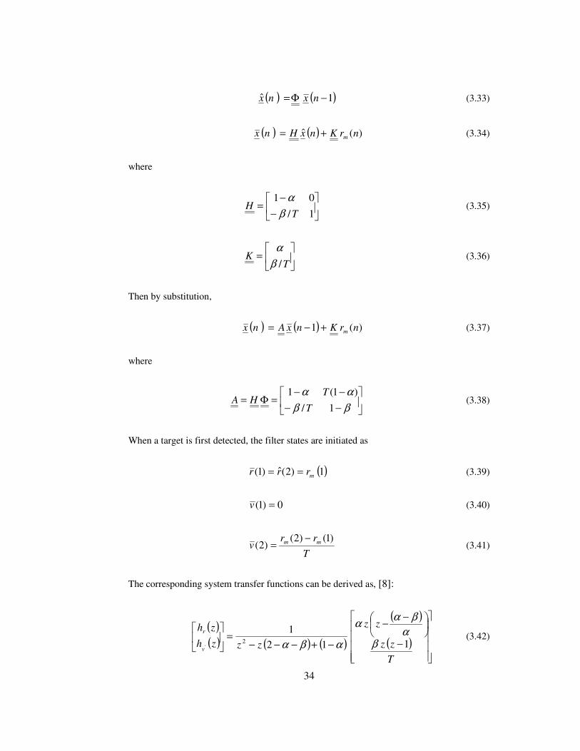
The corresponding system transfer functions can be derived as, [8]:
( )( ) ( ) ( )
( )
( )
−
−−
−+−−−=
T
zz
zz
zzzh
zh
v
r
112
12
' βα
βαα
αβα (3.42)

35
The two poles of the transfer function can be made the same at ξ=z by choosing
21 ξα −= (3.43)
2)1( ξβ −= (3.44)
-2 -1.5 -1 -0.5 0 0.5 1 1.5 2
-1
-0.8
-0.6
-0.4
-0.2
0
0.2
0.4
0.6
0.8
1
Real Part
Imagin
ary
Part
2
Pole/Zero Plot
zeroes
real and
equal
poles
Figure 3-13: Pole-zero plot of the tracking filter with ξ = 0.8.
The poles lie inside the unit circle in the z-plane as long as ξ=z < 1 making the
filter stable. The parameter ξ is called smoothing factor and may be chosen
depending on the tracking requirements. The two poles are real and equal; thus, the
filter is a critically damped (fading memory) filter, [17]. The pole-zero plot of the
filter is shown in Figure 3-13.
In the simulations, the smoothing factor is set to be 0.8. With that setting the filter
has been run separately for simulated input and the convergence results are shown
in Figure 3-14 and Figure 3-15. The simulated input vector consists of the true
range measurements for a target with a constant radial velocity of 50 m/s and the

36
true velocity measurements (constant, 50 m/s). The result for 100 iterations with an
update interval of 0.05 s is shown in Figure 3-14 and Figure 3-15. The initial range
and velocity estimates are set to be off by 50 m and 10 m/s, respectively. That
perturbation serves to display the convergence of the filter. The range error
converges to about 2.5 m, and velocity error converges to 0.
The convergence rate depends on the update interval and the smoothing coefficient.
For more frequent updates and/or smaller values of the smoothing coefficient, the
convergence becomes faster.
0 0.5 1 1.5 2 2.5 3 3.5 4 4.5 51
1.01
1.02
1.03x 10
4 Range track
Time (s)
Range (
m)
Measurements
Estimates
0 0.5 1 1.5 2 2.5 3 3.5 4 4.5 50
20
40
60Range Error
Time (s)
Range (
m)
Figure 3-14: Range performance of the tracking filter; update interval is 0.05 s; smoothing
coefficient is 0.8.

37
0 0.5 1 1.5 2 2.5 3 3.5 4 4.5 550
55
60Velocity track
Time (s)
Velo
city (
m/s
)
Measurements
Estimates
0 0.5 1 1.5 2 2.5 3 3.5 4 4.5 50
5
10Velocity Error
Time (s)
Velo
city (
m/s
)
Figure 3-15: Velocity performance of the tracking filter; update interval is 0.05 s;
smoothing coefficient is 0.8.
3.5 Tracking Performance under No Jamming
A reference run of the developed radar simulator program is presented in this
section. The scenario here does not include jamming pulses or jamming noise. Only
a target return and thermal noise is considered. Simulations for the jamming
scenarios are discussed in detail in Chapter 4.
Received signal during the first snapshot of the track mode is shown in Figure 3-16.
Note that the search mode ends and track mode starts at time instant of 6 ms. Since

38
the radar antenna is directed to the target direction determined in the search mode,
the received pulses have about the same gain.
The initial tracker estimate (range and velocity) is obtained for the simulation by
adding a perturbation to the measurements obtained from the search mode. The
objective of adding a perturbation is to let the tracker to start far from the initial
measurements so as to let the convergence be observed as the tracking filter
converges to a neighborhood of further measurements. A perturbation of 75 m for
range and 10 m/s for velocity is used.
6 6.2 6.4 6.6 6.8 7 7.2 7.4 7.6 7.8 8
x 10-3
0
1
2
3
4
5
6
7
8x 10
-6 Received Signal at First Snapshot
Time (s)
Magnitude
Figure 3-16: Received signal and thermal noise during the first snapshot.

39
The range gate is determined by the initial estimate. The delay measurement is
performed within the range gate as shown in Figure 3-17. The threshold in the
figure is 3.83x10⁻¹⁸. The delay is measured to be 6.65x10⁻⁵ s. Note that the peak
detection algorithm detects the peak in the PSD projection in the lower half of the
figure. Due to noise, however, the location of the peak can vary within the
neighborhood of the true delay of the target. For high input SNR, generally, the data
points above the threshold are the ones due to the samples of the target return pulse.
Thus, the width of that pulse determines the extent of such a neighborhood.
The Doppler measurement is shown in Figure 3-18. The threshold value used for
Doppler detection is 1.0x10⁻¹⁶.
The tracking loop runs until all the snapshots are processed. The number of
snapshots was set to 100 for this particular simulation. The total time span is then 5
s. As a criterion, if the detection stage cannot produce measurements for 3
snapshots (age-out count) in a row, the track is dropped.
Note that the thresholds are determined by using the threshold formula based on the
false alarm rate given by Yt and Yf. The detection threshold is computed such that
the radar receiver maintains a constant pre-determined probability of false alarm
(PFA). The constant false alarm probability in this simulation was set to 10-10. The
value of the false alarm rate is not critical for the analysis here. A lower or a higher
false alarm rate could be used. Increasing the false alarm rate decreases the
threshold levels and more false alarms can appear.
Since the noise power may change during radar operation due to changes in the
environment or due to noise jamming, the threshold is continuously updated based
on the estimates of noise variance for providing a constant PFA value. The process
of continuously changing the threshold value to maintain a constant PFA is called
Constant False Alarm Rate (CFAR) [6].

40
Delay (s)
Dopple
r F
requency (
Hz)
Power Spectral Density
6.2 6.4 6.6 6.8 7 7.2
x 10-5
0
2000
4000
6000
8000
0
0.2
0.4
0.6
0.8
6.2 6.3 6.4 6.5 6.6 6.7 6.8 6.9 7 7.1 7.2
x 10-5
0
2
4
6
x 10-15
Delay (s)
PS
D (
Watt
s)
Projection Along Doppler Onto Delay
Threshold = 3.83e-18
Figure 3-17: PSD of the return signal within the range gate, and its projection on delay axis.
0 1000 2000 3000 4000 5000 6000 7000 8000 9000 100000
0.5
1
1.5
2
2.5
3
3.5
x 10-14
Doppler (Hz)
Pow
er
(Watt
s)
Doppler at delay 6.65e-005 s
Detection:
3.32e+003
Threshold = 1.00e-16
Figure 3-18: Doppler measurement within the first snapshot.

41
In the radar simulator implemented in this thesis, cell-averaging CFAR is used.
Cell averaging is performed on the radar return within the range bins (cells) outside
the range gate. The range gate is about 13 range cells, 6 neighboring range cells on
each side of the current cell. The number of neighboring range cells in a range gate
is a parameter in the simulator program. A CFAR estimate is obtained from the
remaining range cells outside the range gate. With the current settings, a range cell
is about 150 m. Then about 87 remaining range cells outside the range gate in a PRI
are used for the CFAR computation.
The CFAR estimates throughout the snapshots are shown in Figure 3-19. The noise
produced by a random number generator for the simulation had a variance of
2.02x10⁻¹⁴. The CFAR estimates are very close to the true value of the noise power.
0 0.5 1 1.5 2 2.5 3 3.5 4 4.5 51.92
1.94
1.96
1.98
2
2.02
2.04
2.06
2.08
2.1x 10
-14 CFAR Noise Power Estimate
Time (s)
Pow
er
(Watt
s)
Figure 3-19: CFAR noise power estimate throughout the snapshots.

42
Tracking results for the no-jamming case are displayed in Figure 3-20 through
Figure 3-23 together with true range and velocity of the target. The range
measurements and estimates are shown in Figure 3-20. The target's true range
starting at about 10 km is indicated. The measurements are about the true range and
the estimates follow the measurements. The velocity measurements and estimates
are shown Figure 3-21. The velocity measurements are at about 49.8 m/s, which is
close to the target’s constant velocity of 50 m/s within the velocity resolution
dictated by the parameters. The estimates converge to the value of the
measurements. Figure 3-22 and Figure 3-23 display the error in range and velocity
tracks with regard to the true target range and velocity.
The error performance can be quantified by using the root mean square error
(RMS). RMSE is formulated as follows:
∑=
−=s
N
k
kk
s
xxN
RMSE1
21 (3.45)
where kx is the observed value (a range/velocity measurement or estimate), kx is
the true value (true value of range or velocity) and Ns is the number of
measurements (that is, snapshots).
For this reference run, the root mean square error (RMSE) of range and velocity
estimates is 38.9 m and 1.17 m/s respectively and of range and velocity
measurements are 55.1 and 0.2 m/s respectively. RMSE for both quantities are in
the resolution boundaries. Note that the RMSE values are from a single run of the
simulator program. Even though the figures are consistent, a Monte-Carlo
simulation should be run for a large number of noise realizations if more reliable
RMSE figures are desired.

43
0 0.5 1 1.5 2 2.5 3 3.5 4 4.5 50.995
1
1.005
1.01
1.015
1.02
1.025
1.03
1.035x 10
4 Range Measurements and Estimates
Time (s)
Range (
m)
Target Range
Measurements
Estimates
Figure 3-20: Range estimates/measurements for no-jamming tracking scenario.
0 0.5 1 1.5 2 2.5 3 3.5 4 4.5 548
50
52
54
56
58
60Velocity Measurements and Estimates
Time (s)
Velo
city (
m/s
)
Target Velocity
Measurements
Estimates
Figure 3-21: Velocity estimates/measurements for no-jamming tracking scenario.

44
0 0.5 1 1.5 2 2.5 3 3.5 4 4.5 50
20
40
60
80
100
120
140Error in Range Measurements and Estimates
Time (s)
Range E
rror(
m)
Measurements
Estimates
Figure 3-22: Error of range measurements/estimates for no-jamming tracking scenario.
0 0.5 1 1.5 2 2.5 3 3.5 4 4.5 50
1
2
3
4
5
6
7
8
9
10Error in Velocity Measurements and Estimates
Time (s)
Velo
city E
rror
(m/s
)
Measurements
Estimates
Figure 3-23: Error of velocity measurements/estimates for no-jamming tracking scenario.

45
Note that the true range is computed by using the initial range and the constant
velocity of the target. In that respect, it is the theoretical range and velocity of the
target. The simulated target return can be of slightly different range and velocity
values than those from such a calculation due to the quantization errors in the
simulation stage. For instance, a range value of 10 km assigned to a target would
correspond to a return pulse with time-of-arrival index (Matlab indices start from 1)
of 134.33 which is rounded to 134 in the simulation of the received signal (target
return).
A similar representation error occurs for the velocity of the target as well. Such
errors come into picture at the detection stage, that is, they affect the measurements,
as if they are errors emanating from the detection stage. The actual detection errors
are only due to the presence of noise (either thermal noise or spot noise) in the
received signal.
0 0.5 1 1.5 2 2.5 3 3.5 4 4.5 51.005
1.006
1.007
1.008
1.009
1.01
1.011
1.012
1.013x 10
4 Range Measurements and Estimates
Time (s)
Range (
m)
Target Range
Measurements
Estimates
Figure 3-24: Range estimates/measurements for a stationary target at 10050 m.

46
To illustrate this point a stationary target at 10050 m is tracked. The range
measurements and estimates are shown Figure 3-24. The range measurements hop
between 10050 m and 10125 m. The hopping is due the peak detection algorithm as
explained about Figure 3-17. However, there is no range representation error since
the target range, 10050 m, in this example is a multiple of 75 m which is the range
represented by a sampling interval in the simulation. The velocity measurements
(not shown here) are all 0 and estimates converge to the measurements.
A similar simulation is performed for a stationary target at 10075 m, which is not a
multiple of 75 m. The result is shown in Figure 3-25. This time the measurements
still hop between 10050 and 10125 m since the received pulse still is represented by
those sample points in range.
0 0.5 1 1.5 2 2.5 3 3.5 4 4.5 51.005
1.006
1.007
1.008
1.009
1.01
1.011
1.012
1.013x 10
4 Range Measurements and Estimates
Time (s)
Range (
m)
Target Range
Measurements
Estimates
Figure 3-25: Range estimates/measurements for a stationary target at 10075 m.

47
To illustrate that the velocity measurement errors in Figure 3-21 are due to the
reason explained above (the same reason, but for the Doppler frequency
dimension), a simulation is performed similar to that produced results in Figure
3-20 through Figure 3-23, but with velocity set to 50.9765625 m/s. This is a
multiple of the Doppler velocity V∆ that corresponds to the frequency sample
resolution df∆ represented by the 256-point FFT used in the simulations and the
current radar settings. The velocity measurements and estimates are shown
(magnified) in Figure 3-26. The measurements are the same as the true value. Thus
the delay-Doppler detection used in the radar receiver simulator produces correct
measurements, but within quantization errors due to the discrete nature of the
simulated target return, and within errors due to noise (thermal noise or spot-noise
as will be investigated in the next section).
0 0.5 1 1.5 2 2.5 3 3.5 4 4.5 5
50.9765
50.9766
50.9767
50.9768
50.9769
50.977
50.9771
50.9772
50.9773
Velocity Measurements and Estimates
Time (s)
Velo
city (
m/s
)
Target Velocity
Measurements
Estimates
Figure 3-26: Velocity estimates/measurements for a target with no velocity representation
error.

48
CHAPTER 4
4.JAMMING AND ITS EFFECTIVENESS
4.1 The Jamming Concept
Electronic Countermeasure techniques are applied against the radars in order to jam
or deceive the radar receivers. For these purposes, two basic methods are used in the
simulator. These methods consist of noise and range deception which is known as
repeater technique.
4.1.1 Noise Technique
The noise technique is chosen as spot noise which is a narrowband noise technique.
In the simulations, the noise bandwidth is chosen as 5 MHz. The noise is chosen as
Gaussian distributed white noise with variance being equal to the half of the self
protection jammer’s skin paint. The noise is additive on the amplitude of the
received signal. As this simulation model is based on base band, the noise model
has also complex parameters as the received radar signal. The jammer signal skin
paint power is calculated by using the JSR value as specified in the following
formula:
10/10JSRPP rssj = (4.1)
Here, Pr is the received radar echo power and JSR is the jamming to signal ratio in
dB, given as
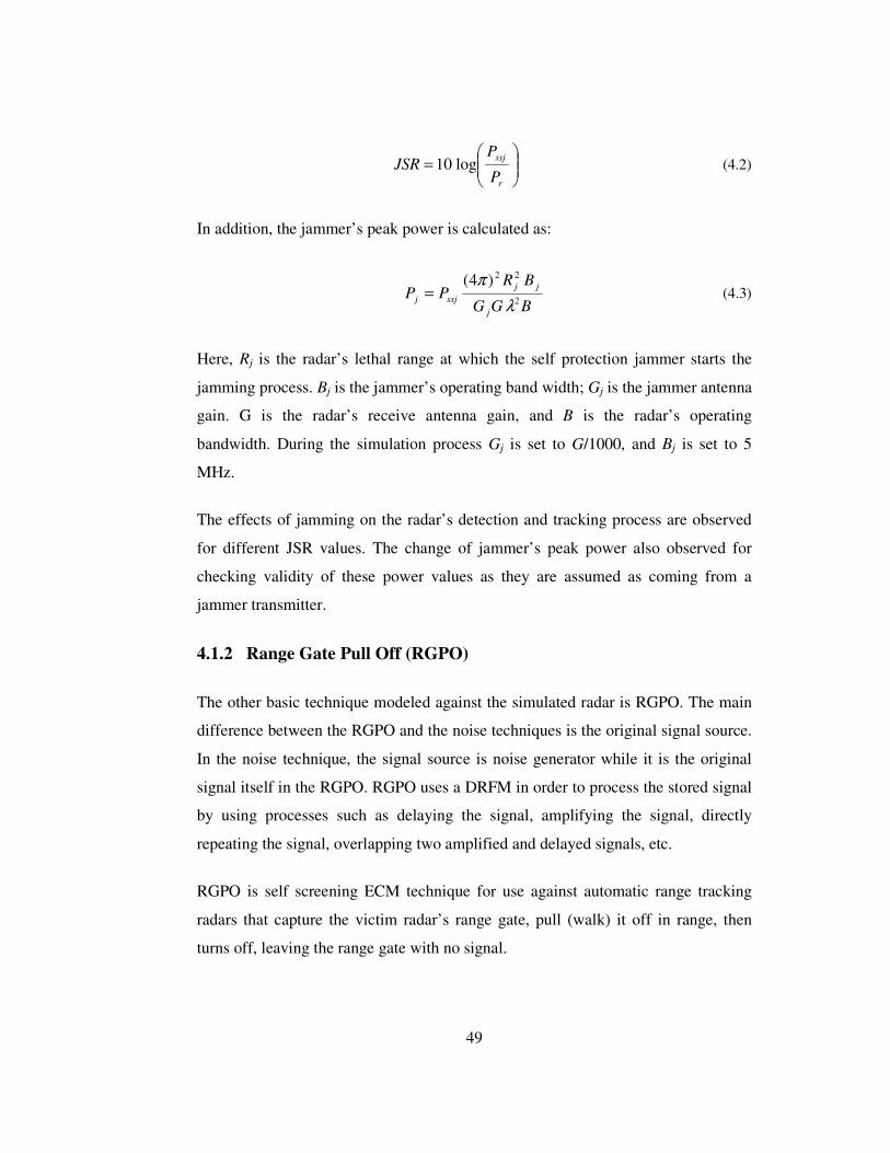
49
=
r
ssj
P
PJSR log10 (4.2)
In addition, the jammer’s peak power is calculated as:
BGG
BRPP
j
jj
ssjj 2
22)4(
λ
π= (4.3)
Here, Rj is the radar’s lethal range at which the self protection jammer starts the
jamming process. Bj is the jammer’s operating band width; Gj is the jammer antenna
gain. G is the radar’s receive antenna gain, and B is the radar’s operating
bandwidth. During the simulation process Gj is set to G/1000, and Bj is set to 5
MHz.
The effects of jamming on the radar’s detection and tracking process are observed
for different JSR values. The change of jammer’s peak power also observed for
checking validity of these power values as they are assumed as coming from a
jammer transmitter.
4.1.2 Range Gate Pull Off (RGPO)
The other basic technique modeled against the simulated radar is RGPO. The main
difference between the RGPO and the noise techniques is the original signal source.
In the noise technique, the signal source is noise generator while it is the original
signal itself in the RGPO. RGPO uses a DRFM in order to process the stored signal
by using processes such as delaying the signal, amplifying the signal, directly
repeating the signal, overlapping two amplified and delayed signals, etc.
RGPO is self screening ECM technique for use against automatic range tracking
radars that capture the victim radar’s range gate, pull (walk) it off in range, then
turns off, leaving the range gate with no signal.

50
Automatic tracking radars, which are used for weapon guidance and fire control
applications, generally employ early and late tracking gates that straddle the return
echo. The gates are removed by a range servo, which follows the target by
predicting its future position using a range gate or velocity estimate developed in
the range tracker. All other returns, except those returned within the tracking gates,
are excluded by the range tracking circuit. This prevents spurious signals from
entering the range tracking circuitry and distorting the range estimate, but it also
offers the opportunity for a deception jammer to operate in a range stealing or track
breaking mode.
RGPO technique causes the radar to get false target range information. This false
target range information can result in significant aiming guidance errors for anti-
aircraft guns and for missiles that use command guidance because the ground-based
computation of weapon lead angle is strongly influenced by the target range as
determined by the radar. However, the tracking radar angle circuitry still functions
to point the radar antenna’s boresight in the direction of the target. This angle
information is sufficient for missile guidance, and hence RGPO by itself is not
sufficient to prevent hits by the weapon system.
The main purposes of the technique are to break the range track circuit of the range
tracking radar.
RGPO is applied against pulsed, automatic, and range tracking radars.
RGPO is generally used with angle jamming techniques. But in the concept of this
simulation, spot noise technique is used together with RGPO.
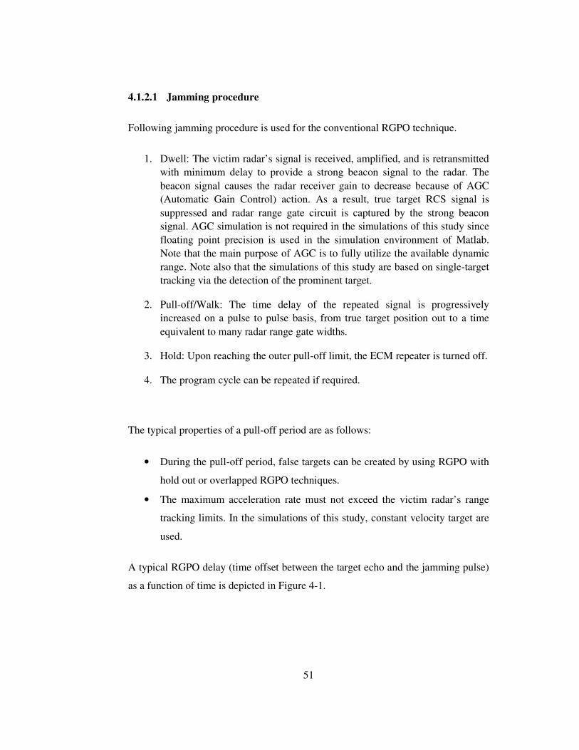
51
4.1.2.1 Jamming procedure
Following jamming procedure is used for the conventional RGPO technique.
1. Dwell: The victim radar’s signal is received, amplified, and is retransmitted with minimum delay to provide a strong beacon signal to the radar. The beacon signal causes the radar receiver gain to decrease because of AGC (Automatic Gain Control) action. As a result, true target RCS signal is suppressed and radar range gate circuit is captured by the strong beacon signal. AGC simulation is not required in the simulations of this study since floating point precision is used in the simulation environment of Matlab. Note that the main purpose of AGC is to fully utilize the available dynamic range. Note also that the simulations of this study are based on single-target tracking via the detection of the prominent target.
2. Pull-off/Walk: The time delay of the repeated signal is progressively increased on a pulse to pulse basis, from true target position out to a time equivalent to many radar range gate widths.
3. Hold: Upon reaching the outer pull-off limit, the ECM repeater is turned off.
4. The program cycle can be repeated if required.
The typical properties of a pull-off period are as follows:
• During the pull-off period, false targets can be created by using RGPO with
hold out or overlapped RGPO techniques.
• The maximum acceleration rate must not exceed the victim radar’s range
tracking limits. In the simulations of this study, constant velocity target are
used.
A typical RGPO delay (time offset between the target echo and the jamming pulse)
as a function of time is depicted in Figure 4-1.

52
Figure 4-1: RGPO Video Programming Waveforms
Figure 4-2: RGPO pulse generation

53
4.1.2.2 ECM parameters
The main parameters in order to define an RGPO technique are as follows:
• Dwell time: This is the time during which cover pulse is to be applied (For
each RGPO cycle it can be set to a different value).
• Pull/Walk time: This is the time during which the TOA of received jamming
pulses walk. It shall walk away from the echo pulse at least at an amount of
ten (10) PW duration. (For each RGPO cycle it may be different)
• Off time: This is the time at which the ECM repeater is turned off upon
reaching the outer pull-off limit, (For each RGPO cycle it can be set to a
different value).
• Pull/Walk time function (parabolic or linear): This function denotes the
change of time delay pattern.
• Number of RGPO cycles: This denotes the number of required RGPO
cycles.
• RGPO cycle period: This is the duration of one RGPO program cycle. This
may be different for each RGPO program cycle.
• Power increment function (parabolic or linear)
o Initial power: This is the power of jamming pulses during dwell.
o Maximum power: This is the maximum power value of jamming pulses gathered at the end of the pull/walk time which should be determined considering the radar receiver limits.
o Slope of the function: This value is slope of power function.
4.1.2.3 Required radar signal parameters
In order to assign an effective jamming technique against a radar mode, one should
know the radar’s receiver characteristics. The transmit parameters like RF, PRI, PW
and modulation type are also required. These parameters can be listed as follows.

54
• Pulse width
• RF frequency, RF frequency set
• PRI, PRI set
• Modulation on pulse train (For instance, Frequency Modulation specifies maximum range of radar)
• Radar’s range tracking circuit limits.
o Maximum range gate speed/ acceleration limit
o Range estimation procedure like Alpha-Beta filter; Alpha-Beta-Gamma filter, Kalman filter.
o Used information for range tracking like Doppler frequency, angle, and etc.
o Band Width
4.1.3 Related Techniques
RGPO type related techniques can be classified as RGPI, Overlapped RGPO, and
RGPO with Hold out (Hook).
4.1.3.1 RGPI
RGPI simulating an inbound target is applied mostly against leading edge range
trackers. In order to apply this technique the repeater should anticipate the reception
of the radar pulse and also have sufficient storage capability to store the radar pulse
for one pulse repetition interval (PRI). For this purpose, the repeater timing should
be initiated from previous received pulse. That is provided by using trackers in the
jammer system.

55
4.1.3.2 Overlapped RGPO
This RGPO program consists of the combination of two RGPO programs one
starting with a delay after the first one is started. This technique creates multiple
range false targets.
4.1.3.3 RGPO with hold out (hook)
This technique is a combination of a hold-out pulse and an RGPO pulse. The
jamming pulse is walked towards the hold-out pulse. When the TOA of the last
jamming pulse matches with the TOA of the hold-out pulse, the pull/walk period is
completed. Like overlapped RGPO, this technique creates multiple range false
targets.

56
4.2 Tracking Performance under Jamming
In this section, the results of tracking simulations performed using jamming pulses
and jamming noise together with the simulated target returns are presented. There
are many radar parameters and subsystems that effect the performance of a tracking
system. Here, we tried to vary only a few parameters that are most relevant to the
respective jamming technique and keep the other parameters the same as of the
tracking simulation without any jamming signal described in Section 3.5.
4.2.1 Spot-Noise Jamming
Here a noise signal is used as the jamming signal. The parameter JSRspn indicating
the amount of jamming noise is varied and tracking results are observed.
Here the subscript spn stands for spot-noise. In RGPO type methods, a jamming
pulse (RGPO, RGPI, etc. pulse) and spot-noise are used together for a certain part
of the jamming period and only the jamming pulse for the rest of the period. The
parameter indicating the jammer-to-signal ratio for the jamming pulses is JSR. It is
kept different from JSRspn to enable assigning separate ratios to jamming pulse and
jamming noise.
The simulation was first run for JSRspn= 6 dB. The number of snapshots is 100 and
the snapshot offset is 0.05 s. The target return and the jamming noise for the last
snapshot and the received signal throughout the snapshots are shown in Figure 4-3.
Note the level of jamming noise and thermal noise. Target range and jammer power
are shown in Figure 4-4 for all snapshots. To satisfy a given JSRspn value for all
instances, the jammer transmit power (and hence jammer received power) is varied
in accordance with the target range. Figure 4-5 shows the CFAR estimate for the
snapshots. CFAR estimate shows a similar declining trend as of the jammer
transmit power.

57
4.956 4.9562 4.9564 4.9566 4.9568 4.957 4.9572 4.9574 4.9576 4.9578 4.9580
0.5
1x 10
-5 Snapshot Target Signal
Time (s)
Magnitude
4.956 4.9562 4.9564 4.9566 4.9568 4.957 4.9572 4.9574 4.9576 4.95780
0.5
1x 10
-5 Snapshot Jamming Signal
Time (s)
Magnitude
0 0.5 1 1.5 2 2.5 3 3.5 4 4.5 50
1
2x 10
-5 Received Signal thru Snapshots
Time (s)
Magnitude
Figure 4-3: Target return and the jamming noise for the last snapshot (Snapshot 100) and
the received signal throughout snapshots. Spot-noise, JSRspn = 6 dB.
0 0.5 1 1.5 2 2.5 3 3.5 4 4.5 51
1.02
1.04x 10
4 Target Range
Time (s)
Range (
m)
0 0.5 1 1.5 2 2.5 3 3.5 4 4.5 50.15
0.16
0.17Jammer Transmit Power
Time (s)
Pow
er
(Watt
s)
0 0.5 1 1.5 2 2.5 3 3.5 4 4.5 53
3.5
4x 10
-12 Jammer Received Power
Time (s)
Pow
er
(Watt
s)
Figure 4-4: Target range, jammer transmit/received power. Spot-noise, JSRspn = 6 dB.

58
0 0.5 1 1.5 2 2.5 3 3.5 4 4.5 53
3.5
4
4.5x 10
-12 CFAR Noise Power Estimate
Time (s)
Pow
er
(Watt
s)
Figure 4-5: CFAR noise power estimate throughout the snapshots. Spot-noise, JSRspn = 6
dB.
6.4 6.6 6.8 7 7.2 7.4
x 10-5
0
2
4
6
x 10-15
Delay (s)
PS
D (
Watt
s)
Projection Along Doppler Onto Delay
Delay (s)
Dopple
r F
requency (
Hz)
Power Spectral Density
6.4 6.6 6.8 7 7.2 7.4
x 10-5
0
2000
4000
6000
8000
0
0.2
0.4
0.6
0.8
Figure 4-6: PSD for the last snapshot of spot-noise jamming simulation for JSRspn = 6 dB.

59
Power spectral density for the last snapshot is shown in Figure 4-6. Note that the
level of the threshold 6.87x10⁻¹⁶ is much higher than that of the no-jamming case,
which is 3.83x10⁻¹⁸. That rise is due to the CFAR estimate of the total noise power
(jamming and thermal components, where the thermal component is relatively quite
small).
Figure 4-7 through Figure 4-10 display the measurement and estimate tracks for
range and velocity. The RMSE for range and velocity estimates are 43.9 m and 1.09
m/s respectively. The RMSE for range and velocity measurements are 58.53 m and
0.28 m/s respectively. Note that the RMSE values are close to those of the no-
jamming case, indicating that the target is being tracked.
The measurement and estimate tracks for range and velocity with the setting
JSRspn= 8 dB are shown in Figure 4-11 through Figure 4-14. The RMSE are slightly
higher but close to that of 6-dB case. For JSRspn= 9 dB, only range tracking result is
shown in Figure 4-15. The track was dropped due to the lack of measurement
updates consecutively, which in turn is due to rising CFAR noise power estimate
that increases the time domain threshold and hence increases the thresholds used in
PSD domain for delay-Doppler measurement. For higher JSRspn values greater than
9 dB, track is dropped much earlier.

60
0 0.5 1 1.5 2 2.5 3 3.5 4 4.5 50.995
1
1.005
1.01
1.015
1.02
1.025
1.03
1.035x 10
4 Range Measurements and Estimates
Time (s)
Range (
m)
Target Range
Measurements
Estimates
Figure 4-7: Spot-noise jamming, JSRspn = 6 dB. Range measurements/estimates.
0 0.5 1 1.5 2 2.5 3 3.5 4 4.5 548
50
52
54
56
58
60Velocity Measurements and Estimates
Time (s)
Velo
city (
m/s
)
Target Velocity
Measurements
Estimates
Figure 4-8: Spot-noise jamming, JSRspn = 6 dB. Velocity measurements/estimates.

61
0 0.5 1 1.5 2 2.5 3 3.5 4 4.5 50
20
40
60
80
100
120Error in Range Measurements and Estimates
Time (s)
Range E
rror(
m)
Measurements
Estimates
Figure 4-9: Spot-noise jamming, JSRspn = 6 dB. Error of range measurements/estimates.
0 0.5 1 1.5 2 2.5 3 3.5 4 4.5 50
1
2
3
4
5
6
7
8
9
10Error in Velocity Measurements and Estimates
Time (s)
Velo
city E
rror
(m/s
)
Measurements
Estimates
Figure 4-10: Spot-noise jamming, JSRspn = 6 dB. Error of velocity measurements/estimates.
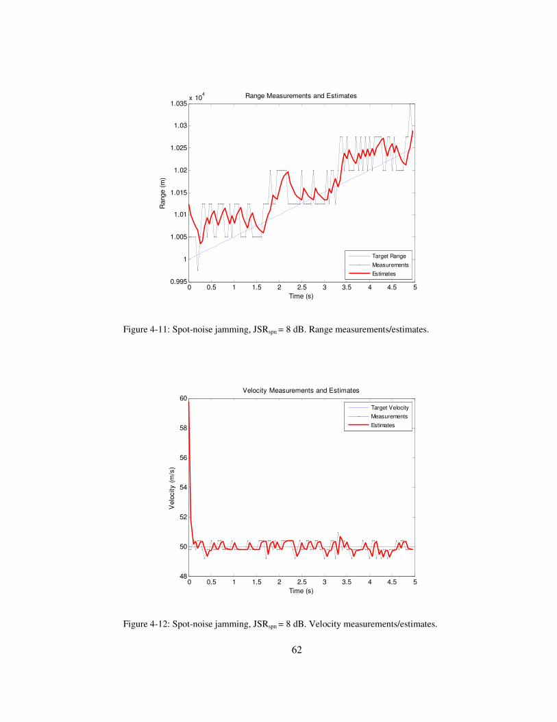
62
0 0.5 1 1.5 2 2.5 3 3.5 4 4.5 50.995
1
1.005
1.01
1.015
1.02
1.025
1.03
1.035x 10
4 Range Measurements and Estimates
Time (s)
Range (
m)
Target Range
Measurements
Estimates
Figure 4-11: Spot-noise jamming, JSRspn = 8 dB. Range measurements/estimates.
0 0.5 1 1.5 2 2.5 3 3.5 4 4.5 548
50
52
54
56
58
60Velocity Measurements and Estimates
Time (s)
Velo
city (
m/s
)
Target Velocity
Measurements
Estimates
Figure 4-12: Spot-noise jamming, JSRspn = 8 dB. Velocity measurements/estimates.

63
0 0.5 1 1.5 2 2.5 3 3.5 4 4.5 50
20
40
60
80
100
120
140Error in Range Measurements and Estimates
Time (s)
Range E
rror(
m)
Measurements
Estimates
Figure 4-13: Spot-noise jamming, JSRspn = 8 dB. Error of range measurements/estimates.
0 0.5 1 1.5 2 2.5 3 3.5 4 4.5 50
1
2
3
4
5
6
7
8
9
10Error in Velocity Measurements and Estimates
Time (s)
Velo
city E
rror
(m/s
)
Measurements
Estimates
Figure 4-14: Spot-noise jamming, JSRspn = 8 dB. Error of velocity measurements/estimates.

64
0 0.5 1 1.5 2 2.5 3 3.5 4 4.5 50.995
1
1.005
1.01
1.015
1.02
1.025x 10
4 Range Measurements and Estimates
Time (s)
Range (
m)
Target Range
Measurements
Estimates
Figure 4-15: Spot-noise jamming, JSRspn = 9 dB. Range measurements/estimates. Track is
dropped due to the lack of measurement updates.
4.2.2 RGPO
Here, a jamming pulse is used together with jamming noise (spot-noise) as the
jamming signal. The jamming pulse first covers the target return (dwell), and then
slowly moves away so that the radar tracks the false target (pull-off) and stops after
certain time (hold). Spot-noise is utilized only for a certain time covering the dwell
and part of pull-off periods. Figure 4-16 displays profiles of such settings as a
function of time. Spot-noise gain is either 1 or 0 indicating presence or absence of
spot noise, respectively. The actual amount of spot-noise is quantified by the

65
parameter JSRspn. Similarly, RGPO gain is different from JSR; it is used to assign
amplitude for the RGPO pulse.
0 5 10 15 20-10
0
10
20
30RGPO Sample Offset
Sam
ple
s
0 5 10 15 201
1.2
1.4
1.6
1.8
RGPO Gain
Gain
0 5 10 15 200
0.5
1RGPO Spot-Noise Gain
Snapshot Start Instants (s)
Gain
0 5 10 15 200
2000
4000
6000
8000RGPO Doppler Offset
Snapshot Start Instants (s)
Hz
Figure 4-16: RGPO offset and gain profiles.
Sample offset is the number of samples the RGPO pulse’s leading edge is displaced
with respect to the leading edge of the target return. In the dwell period, the offset is
set to -1, and the RGPO pulse width is set to be one sample larger than the target
return. Thus an offset of -1 sample lets the RGPO pulse cover the target return fully.
In the pull-off period, the RGPO pulse is pulled away from the target return, and in
the hold section, it is hold at a constant sample offset relative to the target return.

66
Figure 4-17: A typical RGPO sample-offset profile.
A typical RGPO sample-offset profile is shown in Figure 4-17. Slope in the pull-off
period is given by
T
nsRGPO = (4.4)
The slope is positive for RGPO (and negative for RGPI, which is described in the
next section). The amount of range pull-off can be computed as
2
c
sTnRoffset = (4.5)
where Ts is the sampling period. With sTs µ5.0= and smc8103×=
mnRoffset 75×= (4.6)
Then, Doppler velocity and frequency offset are given in terms of the slope as
smssmT
n
T
RV RGPO
offset
offset 7575 ×=== (4.7)

67
HzssV
f RGPORGPOoffset
offsetd 500003.0
7522, ×=
××==
λ (4.8)
In Figure 4-16, RGPOs is 1.3 samples/s. This corresponds to a frequency (Doppler)
offset of 6500 Hz. This is shown in the Doppler offset profile. Note that the range
and velocity of the RGPO pulse are coordinated by this setting. The Doppler offset
of 6500 Hz corresponds to a velocity offset of 97.5 m/s. Adding the target velocity
of 50 m/s to that, the absolute velocity of the false target created by the RGPO pulse
is found to be 147.5 m/s. This corresponds to an absolute Doppler frequency of
9833 Hz, which is the frequency to be measured in the delay-Doppler detection
stage.
For this simulation, the number of snapshots is set to 400 with snapshot offset of
0.05 s, making the total tracking time of the simulation 20 s. The simulation was
first run for JSRspn= 6 dB and JSR = 6 dB. Figure 4-18 through Figure 4-21 display
the PSD in dwell, pull-off and hold periods. Note that the Doppler frequency of the
jamming pulse in PSD suits the Doppler offset profile.
The CFAR estimates throughout the snapshots in Figure 4-22 indicate the presence
of spot-noise for the duration it was applied, thermal noise (the reading around
2x10-14 from the plot matches the actual noise power used) and the target return
moving out of the range gate as the radar receiver follows the RGPO pulse.
The measurement and estimate tracks are shown in Figure 4-23 and Figure 4-24.
The pull-off in the range dimension was successful. The resulting RMSE was about
961.4 m and 92.3 m/s for range and velocity estimates, and 968.1 m and 92.4 m/s
for range and velocity measurements. The RMSE values also indicate a successful
false target creation using the RGPO jamming. Note that the estimates closely track
the measurements.

68
Delay (s)
Dopple
r F
requency (
Hz)
Power Spectral Density
6.2 6.4 6.6 6.8 7 7.2
x 10-5
0
2000
4000
6000
8000
0
0.2
0.4
0.6
0.8
6.2 6.3 6.4 6.5 6.6 6.7 6.8 6.9 7 7.1 7.2
x 10-5
0
2
4
6
x 10-15
Delay (s)
PS
D (
Watt
s)
Projection Along Doppler Onto Delay
Figure 4-18: RGPO. Snapshot 1, cover pulse. Spot-noise present. sRGPO = 1.3 samples/s.
6.6 6.8 7 7.2 7.4 7.6
x 10-5
0
1
2
3
x 10-14
Delay (s)
PS
D (
Watt
s)
Projection Along Doppler Onto Delay
Delay (s)
Dopple
r F
requency (
Hz)
Power Spectral Density
6.6 6.8 7 7.2 7.4 7.6
x 10-5
0
2000
4000
6000
8000 0.2
0.4
0.6
0.8
Figure 4-19: RGPO. Snapshot 108, jamming pulse starts pull-off. Spot-noise present.
sRGPO = 1.3 samples/s.

69
7 7.2 7.4 7.6 7.8 8
x 10-5
0
2
4
6
x 10-14
Delay (s)
PS
D (
Watt
s)
Projection Along Doppler Onto Delay
Delay (s)
Dopple
r F
requency (
Hz)
Power Spectral Density
7 7.2 7.4 7.6 7.8 8
x 10-5
0
2000
4000
6000
8000
0
0.2
0.4
0.6
0.8
Figure 4-20: RGPO. Snapshot 203, further in pull-off. Spot-noise not present. sRGPO = 1.3
samples/s.
7.9 8 8.1 8.2 8.3 8.4 8.5 8.6 8.7 8.8 8.9
x 10-5
0
0.5
1
x 10-13
Delay (s)
PS
D (
Watt
s)
Projection Along Doppler Onto Delay
Delay (s)
Dopple
r F
requency (
Hz)
Power Spectral Density
8 8.2 8.4 8.6 8.8 9
x 10-5
0
2000
4000
6000
8000 0.2
0.4
0.6
0.8
Figure 4-21: RGPO. Snapshot 384, hold period. Spot-noise not present. sRGPO = 1.3
samples/s.

70
0 2 4 6 8 10 12 14 16 18 200
0.5
1
1.5
2
2.5
3
3.5
4
4.5x 10
-12 CFAR Noise Power Estimate
Time (s)
Pow
er
(Watt
s)
spot-noise
thermal
noise target return outside
the range gate
Figure 4-22: RGPO. CFAR noise power estimate. sRGPO = 1.3 samples/s.

71
0 2 4 6 8 10 12 14 16 18 200.95
1
1.05
1.1
1.15
1.2
1.25
1.3x 10
4 Range Measurements and Estimates
Time (s)
Range (
m)
Target Range
Estimates
Measurements
RGPO Range
Figure 4-23: RGPO. Range measurements/estimates. JSRspn= 6 dB, JSR = 6 dB, sRGPO = 1.3
samples/s.
RGPO Range
Target Range

72
0 2 4 6 8 10 12 14 16 18 2040
60
80
100
120
140
160Velocity Measurements and Estimates
Time (s)
Velo
city (
m/s
)
Target Velocity
Estimates
Measurements
Figure 4-24: RGPO. Velocity measurements/estimates. JSRspn= 6 dB, JSR = 6 dB, sRGPO =
1.3 samples/s.

73
A similar simulation was performed but with JSR = -6 dB. The range tracking
performance is shown in Figure 4-25 and Figure 4-26. The radar tracks the actual
target for a while and starts to track the false target as the false target’s pulse
amplitude becomes higher than that of the target return. The same tracking behavior
is observed for velocity in Figure 4-27.
0 2 4 6 8 10 12 14 16 18 200.95
1
1.05
1.1
1.15
1.2
1.25
1.3x 10
4 Range Measurements and Estimates
Time (s)
Range (
m)
Target Range
Estimates
Measurements
RGPO Range
Figure 4-25: RGPO. Range measurements/estimates. JSRspn= 6 dB, JSR = -6 dB, sRGPO =
1.3 samples/s.
RGPO Range Target
Range

74
8 9 10 11 12 13 141.02
1.04
1.06
1.08
1.1
1.12
1.14
1.16
1.18x 10
4 Range Measurements and Estimates
Time (s)
Range (
m)
Target Range
Estimates
Measurements
RGPO Range
Figure 4-26: Close-up of Figure 4-25.
Target Range
RGPO Range

75
0 2 4 6 8 10 12 14 16 18 2040
60
80
100
120
140
160Velocity Measurements and Estimates
Time (s)
Velo
city (
m/s
)
Target Velocity
Estimates
Measurements
Figure 4-27: RGPO. Velocity measurements/estimates. JSRspn= 6 dB, JSR = -6 dB, sRGPO =
1.3 samples/s.

76
The results of a simulation with all the same parameters but with JSR = -7 dB is
shown in Figure 4-28 and Figure 4-29. The jamming pulse is now even smaller than
the actual target return, and the radar tracks the actual target.
Note the effect of spot noise used in the first 10 s of tracking is apparent in Figure
4-29. This is because the detected peak in this case is that of the target return and
the target return is relatively smaller in amplitude with respect to spot noise than the
jammer pulses of the previous cases.
0 2 4 6 8 10 12 14 16 18 200.95
1
1.05
1.1
1.15
1.2
1.25
1.3x 10
4 Range Measurements and Estimates
Time (s)
Range (
m)
Target Range
Estimates
Measurements
RGPO Range
Figure 4-28: RGPO. Range measurements/estimates. JSRspn= 6 dB, JSR = -7 dB, sRGPO =
1.3 samples/s.
Target Range
RGPO Range

77
0 2 4 6 8 10 12 14 16 18 2048
50
52
54
56
58
60Velocity Measurements and Estimates
Time (s)
Velo
city (
m/s
)
Target Velocity
Estimates
Measurements
Figure 4-29: RGPO. Velocity measurements/estimates. JSRspn= 6 dB, JSR = -7 dB, sRGPO =
1.3 samples/s.
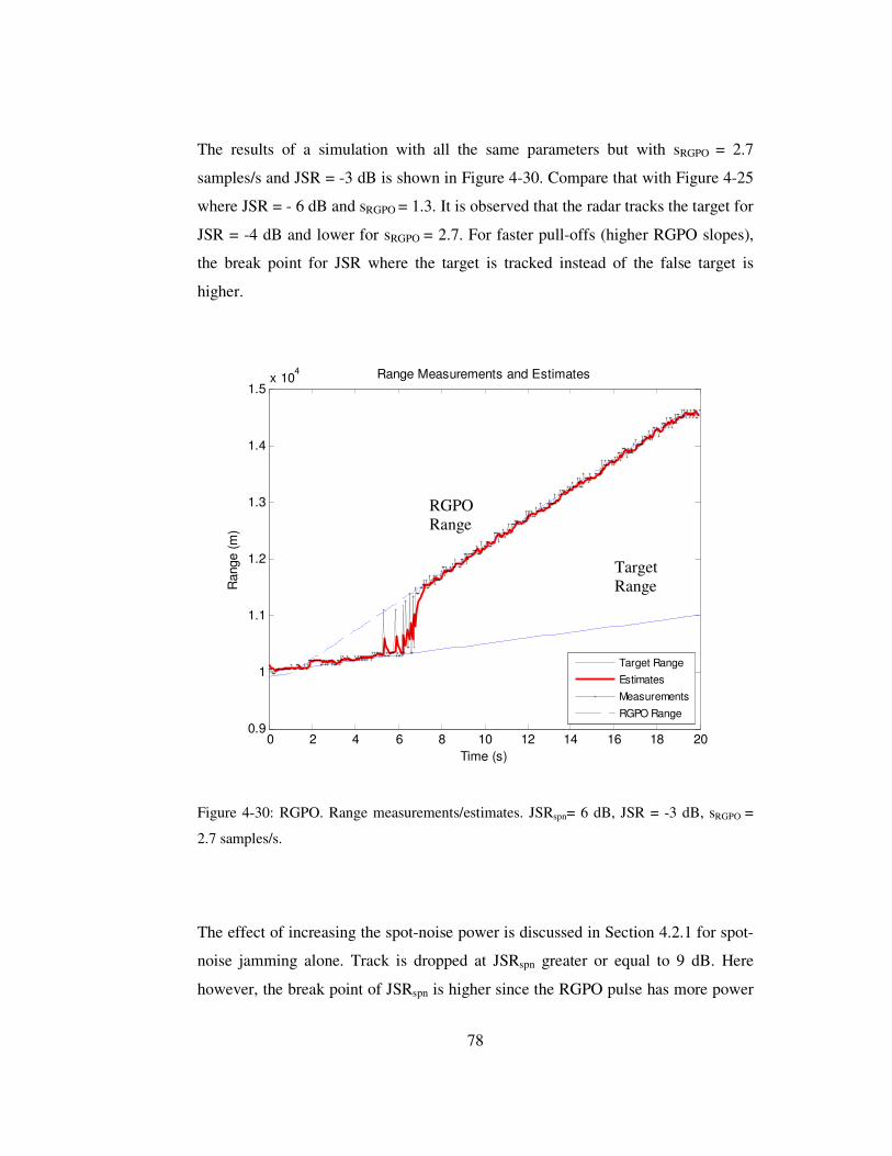
78
The results of a simulation with all the same parameters but with sRGPO = 2.7
samples/s and JSR = -3 dB is shown in Figure 4-30. Compare that with Figure 4-25
where JSR = - 6 dB and sRGPO = 1.3. It is observed that the radar tracks the target for
JSR = -4 dB and lower for sRGPO = 2.7. For faster pull-offs (higher RGPO slopes),
the break point for JSR where the target is tracked instead of the false target is
higher.
0 2 4 6 8 10 12 14 16 18 200.9
1
1.1
1.2
1.3
1.4
1.5x 10
4 Range Measurements and Estimates
Time (s)
Range (
m)
Target Range
Estimates
Measurements
RGPO Range
Figure 4-30: RGPO. Range measurements/estimates. JSRspn= 6 dB, JSR = -3 dB, sRGPO =
2.7 samples/s.
The effect of increasing the spot-noise power is discussed in Section 4.2.1 for spot-
noise jamming alone. Track is dropped at JSRspn greater or equal to 9 dB. Here
however, the break point of JSRspn is higher since the RGPO pulse has more power
Target Range
RGPO Range

79
than the target return. In a simulation with all the parameters the same as that of
Section 4.2.1, this break point was observed to be JSRspn=12 dB.
On the other hand, varying the parameter JSR has almost no effect as far as the
jamming pulse is higher in peak amplitude in the PSD domain than the target return.
This is because of the modeled radar receiver which detects the prominent return
(single-target-detection) as the target to track.
In general, it is important how fast the RGPO pulse is pulled off and whether the
tracking filter can follow. The former depends on the steepness of the sample-offset
slope, that is, sRGPO; and the latter depends on the tracking filter’s smoothing
coefficient and the measurement update interval. If a large (close to 1, e.g. 0.98)
smoothing coefficient together with a large update interval (e.g. 0.4 s) is used, the
tracking filter is slow in convergence. The slope sRGPO about 3 samples/s is a fast
pull-off and it is observed that the track is dropped. In the simulations presented in
this section, a smoothing coefficient of 0.8 and an update interval of 0.05 s are used.
Thus the filter is fast enough not to cause any track-drops with even much higher
sRGPO values than 3 samples/s.
It is also observed that for even higher values of the slope (e.g. 30 samples/s) and
with a fast-converging tracking filter, the radar cannot track the fast false target, but
instead locks on the actual target.
4.2.3 RGPI
RGPI is very similar to RGPO. The jamming pulse is pulled in instead of being
pulled off. A simulation was performed for the case with offset and gain profiles
shown in Figure 4-31 and JSRspn= 6 dB and JSR= 6 dB. Note the RGPI slope is
negative and is -1.3 samples/s. Note also that the Doppler offset is wrapped around

80
as 10 kHz-1.3 x 5000Hz= 3500 Hz. This corresponds to a velocity offset of 52.5
m/s; and an absolute velocity of 102.5 m/s, with the target’s true velocity being 50
m/s.
The PSD for Snapshot 108, 170 and 384 is shown in Figure 4-32, Figure 4-33, and
Figure 4-34, respectively. The measurement and estimate tracks are shown in
Figure 4-35 and Figure 4-36. The radar tracks the false RGPI target both in range
and velocity; and hence the false target creation is successful.
The results of similar simulations but with JSR set to -5 dB and -6 dB are shown in
Figure 4-37 and Figure 4-38, respectively. For – 5 dB, the radar tracks the target for
a while and switches to the false target as the pulse amplitude of the false target gets
larger. For -6 dB, the radar tracks the actual target.
The observation on tracking performance with steeper RGPI slopes is the same as
of the RGPO in the previous section. With a slowly converging tracking filter and
steeper slopes, the track is dropped. Also, for even steeper slopes (e.g. -20
samples/s) and with a fast-converging tracking filter, the radar cannot track the fast
false target, but instead locks on the actual target.

81
0 5 10 15 20-30
-20
-10
0RGPI Sample Offset
Sam
ple
s
0 5 10 15 201
1.2
1.4
1.6
1.8
RGPI Gain
Gain
0 5 10 15 200
0.5
1RGPI Spot-Noise Gain
Snapshot Start Instants (s)
Gain
0 5 10 15 200
1000
2000
3000
4000RGPI Doppler Offset
Snapshot Start Instants (s)H
z
Figure 4-31: RGPI offset and gain profiles.
6 6.1 6.2 6.3 6.4 6.5 6.6 6.7 6.8 6.9 7
x 10-5
0
1
2
3
x 10-14
Delay (s)
PS
D (
Watt
s)
Projection Along Doppler Onto Delay
Delay (s)
Dopple
r F
requency (
Hz)
Power Spectral Density
6 6.2 6.4 6.6 6.8 7
x 10-5
0
2000
4000
6000
8000
0
0.2
0.4
0.6
0.8
Figure 4-32: RGPI. Snapshot 108, jamming pulse starts pulling in. Spot-noise present. sRGPI
= -1.3 samples/s.

82
5.9 6 6.1 6.2 6.3 6.4 6.5 6.6 6.7 6.8 6.9
x 10-5
0
2
4
x 10-14
Delay (s)
PS
D (
Watt
s)
Projection Along Doppler Onto Delay
Delay (s)
Dopple
r F
requency (
Hz)
Power Spectral Density
6 6.2 6.4 6.6 6.8 7
x 10-5
0
2000
4000
6000
8000
0
0.2
0.4
0.6
0.8
Figure 4-33: RGPI. Snapshot 170, further in pull-in. Spot-noise present. sRGPI = -1.3
samples/s.
5.6 5.7 5.8 5.9 6 6.1 6.2 6.3 6.4 6.5 6.6
x 10-5
0
0.5
1
x 10-13
Delay (s)
PS
D (
Watt
s)
Projection Along Doppler Onto Delay
Delay (s)
Dopple
r F
requency (
Hz)
Power Spectral Density
5.6 5.8 6 6.2 6.4 6.6
x 10-5
0
2000
4000
6000
8000 0.2
0.4
0.6
0.8
Figure 4-34: RGPI. Snapshot 384, hold period. Spot-noise not present. sRGPI = -1.3
samples/s.

83
0 2 4 6 8 10 12 14 16 18 200.9
0.92
0.94
0.96
0.98
1
1.02
1.04
1.06
1.08
1.1x 10
4 Range Measurements and Estimates
Time (s)
Range (
m)
Target Range
Estimates
Measurements
RGPI Range
Figure 4-35: RGPI. Range measurements/estimates. JSRspn= 6 dB, JSR = 6 dB, sRGPI = -1.3
samples/s.
Target Range
RGPI Range

84
0 2 4 6 8 10 12 14 16 18 2040
50
60
70
80
90
100
110Velocity Measurements and Estimates
Time (s)
Velo
city (
m/s
)
Target Velocity
Estimates
Measurements
Figure 4-36: RGPI. Velocity measurements/estimates. JSRspn= 6 dB, JSR = 6 dB, sRGPI = -
1.3 samples/s.
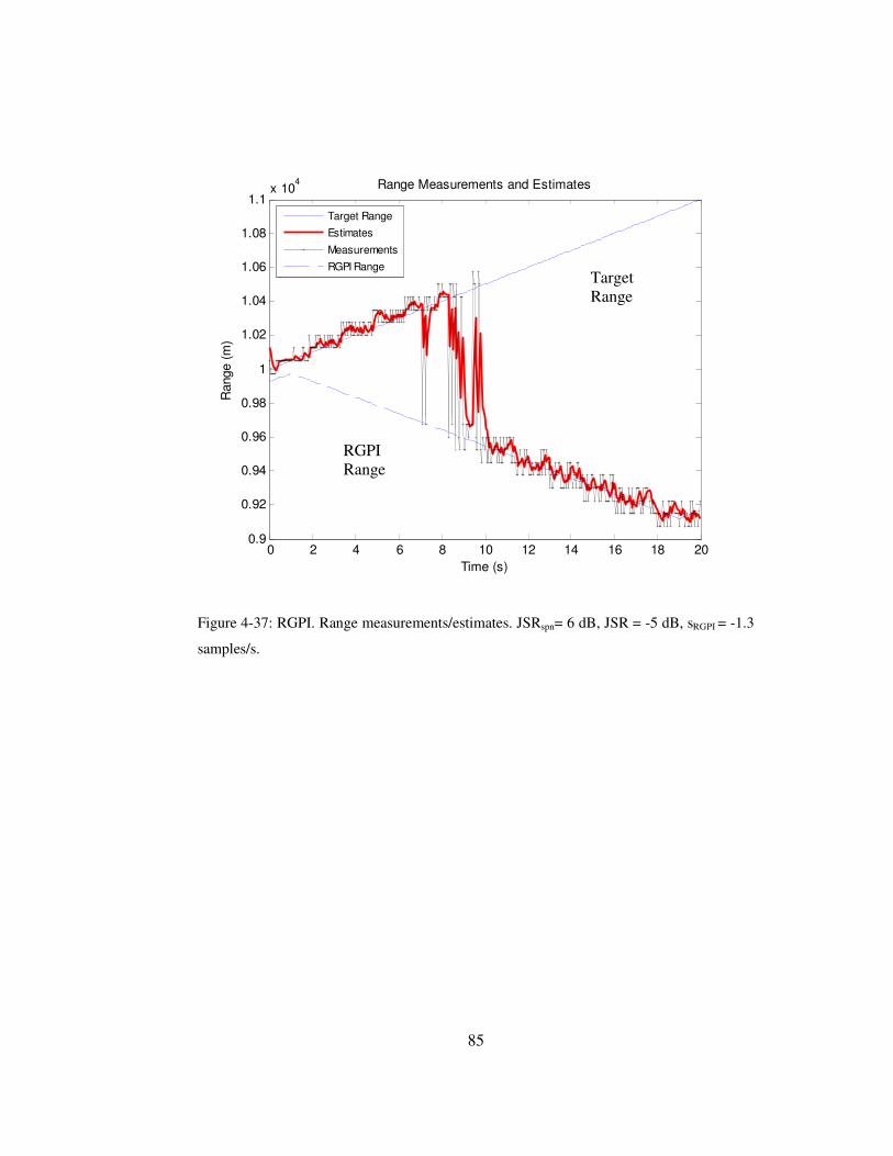
85
0 2 4 6 8 10 12 14 16 18 200.9
0.92
0.94
0.96
0.98
1
1.02
1.04
1.06
1.08
1.1x 10
4 Range Measurements and Estimates
Time (s)
Range (
m)
Target Range
Estimates
Measurements
RGPI Range
Figure 4-37: RGPI. Range measurements/estimates. JSRspn= 6 dB, JSR = -5 dB, sRGPI = -1.3
samples/s.
Target Range
RGPI Range

86
0 2 4 6 8 10 12 14 16 18 200.9
0.95
1
1.05
1.1
1.15x 10
4 Range Measurements and Estimates
Time (s)
Range (
m)
Target Range
Estimates
Measurements
RGPI Range
Figure 4-38: RGPI. Range measurements/estimates. JSRspn= 6 dB, JSR = -6 dB, sRGPI = -1.3
samples/s.
4.2.4 Overlapped RGPO
Here two jamming pulses are used instead of one as in RGPO technique. The offset
and gain profiles overlap as shown in Figure 4-39, which displays the profiles for
the RGPO pulse and Figure 4-40, which displays profiles for overlapping RGPO
pulse. Usually the overlapping pulse starts later in time. Here the overlapping pulse
appears 0.5 s later than the RGPO pulse since the pulse gain for the overlapping
pulse is 0 for the first 0.5 s.
Target Range
RGPI Range

87
0 5 10 15 20-20
0
20
40
60RGPO Sample Offset
Sam
ple
s
0 5 10 15 201
1.2
1.4
1.6
1.8
RGPO Gain
Gain
0 5 10 15 200
0.5
1RGPO Spot-Noise Gain
Snapshot Start Instants (s)
Gain
0 5 10 15 200
1000
2000
3000
4000RGPO Doppler Offset
Snapshot Start Instants (s)H
z
Figure 4-39: RGPO offset and gain profiles. sRGPO = 2.7 samples/s.
0 5 10 15 20-10
0
10
20
30OVLP-RGPO Sample Offset
Sam
ple
s
0 5 10 15 200
0.5
1
1.5OVLP-RGPO Gain
Gain
0 5 10 15 20-1
-0.5
0
0.5
1OVLP-RGPO Spot-Noise Gain
Snapshot Start Instants (s)
Gain
0 5 10 15 200
2000
4000
6000
8000OVLP-RGPO Doppler Offset
Snapshot Start Instants (s)
Hz
Figure 4-40: Overlapping RGPO pulse's offset and gain profiles. sOVLP-RGPO = 1.3 samples/s.

88
The slopes in pull-off periods are 2.7 samples/s and 1.3 samples/s for the RGPO
pulse and overlapping pulse, respectively. The RGPO pulse is pulled off faster.
Note that the Doppler offset profile for RGPO is wrapped around (modulo 10 kHz)
in frequency. The velocity offsets for RGPO and overlapping RGPO pulse can be
calculated as 2.7 x 5000 Hz – 10 kHz = 3500 Hz and 1.3 x 5000 Hz = 6500 Hz
respectively. The corresponding absolute velocities are 102.5 m/s and 147.5 m/s,
respectively. Note that even though the RGPO pulse is pulled off faster, its velocity
to be measured is less than that of the overlapping RGPO pulse due to the frequency
wrapping in the Doppler frequency dimension.
A simulation was run for JSRspn = 6 dB and JSR = 6 dB. Figure 4-41 and Figure
4-42 display the tracking results for range and velocity, respectively. The radar
measurements hop between the RGPO and overlapped RGPO pulses for a while but
eventually the radar tracks the false target created by the RGPO pulse in range and
velocity.
The reason for the hopping in the measurements is that the overlapped RGPO and
RGPO pulses have almost the same but slightly different gains due to the presence
of thermal noise and due to the 0.5 s offset between the respective gain profiles.
Since the detection stage performs a peak detection (single-target detection),
whichever pulse has a higher peak in the PSD domain is assigned to be the one
producing the measurement.
Figure 4-43 and Figure 4-44 display the range measurements and estimates for
simulations with all parameters the same but JSR set to be -6 dB and -7 dB,
respectively. Compare those with Figure 4-25 and Figure 4-28, where similar
results for an RGPO pulse with sRGPO = 1.3 samples/s are displayed. Thus, the
overlapped RGPO is not much different from RGPO. Depending on the peak value
in the PSD in the detection stage, the radar tracks either the target or the false
targets created by RGPO or overlapped RGPO pulses.

89
0 2 4 6 8 10 12 14 16 18 200.9
1
1.1
1.2
1.3
1.4
1.5x 10
4 Range Measurements and Estimates
Time (s)
Range (
m)
Target Range
Estimates
Measurements
RGPO Range
Overlap Range
Figure 4-41: Overlapped RGPO. Range measurements/estimates. JSRspn= 6 dB, JSR = 6
dB, sRGPO = 2.7 samples/s, sOVLP-RGPO = 1.3 samples/s.
RGPO Range OVLP-RGPO
Range
Target Range

90
0 2 4 6 8 10 12 14 16 18 2040
60
80
100
120
140
160Velocity Measurements and Estimates
Time (s)
Velo
city (
m/s
)
Target Velocity
Estimates
Measurements
Figure 4-42: Overlapped RGPO. Velocity measurements/estimates. JSRspn= 6 dB, JSR = 6
dB, sOVLP-RGPO = 2.7 samples/s. sRGPO = 1.3 samples/s.

91
0 2 4 6 8 10 12 14 16 18 200.9
1
1.1
1.2
1.3
1.4
1.5x 10
4 Range Measurements and Estimates
Time (s)
Range (
m)
Target Range
Estimates
Measurements
RGPO Range
Overlap Range
Figure 4-43: Overlapped RGPO. Range measurements/estimates. JSRspn= 6 dB, JSR = -6
dB, sRGPO = 2.7 samples/s, sOVLP-RGPO = 1.3 samples/s.
Target Range
RGPO Range
OVLP-RGPO Range

92
0 2 4 6 8 10 12 14 16 18 200.9
1
1.1
1.2
1.3
1.4
1.5x 10
4 Range Measurements and Estimates
Time (s)
Range (
m)
Target Range
Estimates
Measurements
RGPO Range
Overlap Range
Figure 4-44: Overlapped RGPO. Range measurements/estimates. JSRspn= 6 dB, JSR = -7
dB, sRGPO = 2.7 samples/s, sOVLP-RGPO = 1.3 samples/s.
4.2.5 RGPO with hold-out
This technique is similar to overlapped RGPO with the difference that the
overlapping pulse stands at the same location and does not move relative to the
target return. The RGPO pulse is pulled off towards the hold-out pulse and they
fully overlap in the hold period.
A simulation was run for JSRspn = 6 dB and JSR = 6 dB. The offset and gain profiles
are shown in Figure 4-45 and Figure 4-46. The pull-off slope of the RGPO pulse is
1.3 samples/s.
Target Range
OVLP-RGPO Range
RGPO Range

93
0 5 10 15 20-10
0
10
20
30RGPO Sample Offset
Sam
ple
s
0 5 10 15 201
1.2
1.4
1.6
1.8
RGPO Gain
Gain
0 5 10 15 200
0.5
1RGPO Spot-Noise Gain
Snapshot Start Instants (s)
Gain
0 5 10 15 200
2000
4000
6000
8000RGPO Doppler Offset
Snapshot Start Instants (s)
Hz
Figure 4-45: RGPO with hold-out. RGPO offset and gain profiles. sRGPO = 1.3 samples/s.
0 5 10 15 2021
22
23
24RGPO-HO Sample Offset
Sam
ple
s
0 5 10 15 200
1
2
3RGPO-HO Gain
Gain
0 5 10 15 20-1
-0.5
0
0.5
1RGPO-HO Spot-Noise Gain
Snapshot Start Instants (s)
Gain
0 5 10 15 20-1
-0.5
0
0.5
1RGPO-HO Doppler Offset
Snapshot Start Instants (s)
Hz
Figure 4-46: RGPO with hold-out. Hold-out offset and gain profiles.

94
The measurement and estimate tracks are shown in Figure 4-47 and Figure 4-48. As
soon as the hold-out pulse moves into the range gate, the radar starts to track the
false target due to the hold-out pulse. The hold-out gain is set to be a constant, while
the gain of the RGPO pulse slowly increases to that constant. Thus, when the range
gate advances to include the hold-out pulse, the gain of the RGPO pulse is lower,
and because of the single-target detection implemented in the simulator, the radar
detects the hold-out pulse as the prominent target. As long as either the RGPO pulse
or the hold-out pulse has higher peaks in the PSD domain than that of the target
return, the radar locks on the false target.
Since the hold-out pulse does not move relative to the target return, its relative
velocity is 0. Thus, the absolute velocity measurements are 50 m/s, the same as that
of the target, as the hold-out pulse is being tracked.
The result of a simulation with all the parameters kept the same but with JSR = -6
dB is shown in Figure 4-49. Similar to the results of the RGPO in Section 4.2.2, the
radar tracks the false target after tracking the actual target for a while. However, this
time, radar tracks the hold-out pulse as governed by the gains set to RGPO and
hold-out pulses. The radar tracks the actual target for JSR = -7 dB and lower. The
case with JSR = - 7 dB is shown in Figure 4-50.
The result of a simulation with JSR = -3 dB and the pull-off slope of the RGPO
pulse set to 2.7 samples/s is shown in Figure 4-51. Compare this to Figure 4-30 for
a similar result. Here, the radar tracks the target for a while, switches to the false
target due to RGPO pulse and then locks onto the false target due to the hold-out
pulse.

95
0 2 4 6 8 10 12 14 16 18 200.95
1
1.05
1.1
1.15
1.2
1.25
1.3x 10
4 Range Measurements and Estimates
Time (s)
Range (
m)
Target Range
Estimates
Measurements
RGPO Range
Hold-out Range
Figure 4-47: RGPO with hold-out. Range measurements/estimates. JSRspn= 6 dB, JSR = 6
dB, sRGPO = 1.3 samples/s.
RGPO Range
Hold-out Range
Target Range

96
0 2 4 6 8 10 12 14 16 18 2040
60
80
100
120
140
160Velocity Measurements and Estimates
Time (s)
Velo
city (
m/s
)
Target Velocity
Estimates
Measurements
Figure 4-48: RGPO with hold-out. Velocity measurements/estimates. JSRspn= 6 dB, JSR =
6 dB, sRGPO = 1.3 samples/s.

97
0 2 4 6 8 10 12 14 16 18 200.95
1
1.05
1.1
1.15
1.2
1.25
1.3x 10
4 Range Measurements and Estimates
Time (s)
Range (
m)
Target Range
Estimates
Measurements
RGPO Range
Hold-out Range
Figure 4-49: RGPO with hold-out. Range measurements/estimates. JSRspn= 6 dB, JSR = -6
dB, sRGPO = 1.3 samples/s.
Hold-out Range
RGPO Range
Target Range

98
0 2 4 6 8 10 12 14 16 18 200.95
1
1.05
1.1
1.15
1.2
1.25
1.3x 10
4 Range Measurements and Estimates
Time (s)
Range (
m)
Target Range
Estimates
Measurements
RGPO Range
Hold-out Range
Figure 4-50: RGPO with hold-out. Range measurements/estimates. JSRspn= 6 dB, JSR = -7
dB, sRGPO = 1.3 samples/s.
Hold-out Range
RGPO Range
Target Range

99
0 2 4 6 8 10 12 14 16 18 200.9
1
1.1
1.2
1.3
1.4
1.5x 10
4 Range Measurements and Estimates
Time (s)
Range (
m)
Target Range
Estimates
Measurements
RGPO Range
Hold-out Range
Figure 4-51: RGPO with hold-out. Range measurements/estimates. JSRspn= 6 dB, JSR = -3
dB, sRGPO = 2.7 samples/s.
Target Range
RGPO Range
Hold-out Range

100
CHAPTER 5
5.CONCLUSIONS
Self protection electronic warfare systems require effective jamming techniques.
The most critical point in designing a jamming technique is to have detailed
information about the receiver characteristics of the threat radars. Simulation of a
radar receiver thus enables a fast and comprehensive evaluation of jamming
techniques' effectiveness against various threat radars given their receiver
characteristics.
In this study, we simulated a radar receiver based on a certain radar model that
includes a multiple-target search and single-target track functionality. The
simulation also includes a jamming signal simulator that can be used to investigate
the effectiveness of a number of different jamming techniques on the simulated
radar model in regard to target detection and tracking performance.
The radar model is of pulse-Doppler. A sector scanning receiver antenna in the
search mode and a fixed directive receiver antenna in the single-target track mode
are assumed. Various radar parameters and the geometry of the scenario such as
antenna pattern, received power, range variations of the targets are all included in
the model. The detection of targets produces range, Doppler velocity and azimuth
angle of each target. The radar turns its antenna towards the direction of one of the
targets that is decided to be tracked. Then the tracking algorithm that is incorporated
into the simulation tracks the target throughout its course. When the jamming
signals are included in the simulation, the effectiveness of the jamming technique

101
that is being used can be investigated by observing its effects in detection and
tracking.
The employed jamming techniques include noise jamming (spot-noise) and RGPO
based techniques. Variations of RGPO such as RGPO with hold-out and overlapped
RGPO techniques are developed and investigated. RGPO techniques use spot-noise
as well in the dwell and in part of the pulse pulling periods. The jamming
effectiveness is evaluated for varying jamming-to-signal ratios (JSR). For better
identifying the effectiveness of the jamming noise and jamming pulse separately,
separate parameters, JSRspn and JSR, respectively, are used to vary the strength of
the jammer components.
Jamming performance of spot noise is dependent on the parameter JSRspn. For the
parameter larger than a certain value, the track is dropped and the radar cannot track
the target. For values smaller than that break point, the radar can track the target.
The value of the break point depends on the radar parameters used such as the
measurement update interval (snapshot offset) and tracking filter’s smoothing
coefficient; and can be evaluated easily by using the simulator program developed
in this study. With the parameters used in this thesis, the break point is found to be
9 dB.
For the RGPO technique and its variations, the effectiveness is determined by JSR,
which determines the strength of the jamming pulse. The pulse amplitudes in
techniques of overlapped RGPO and RGPO with hold-out are adjusted by using
separate gain coefficients, in addition to a common value of the parameter JSR, for
RGPO pulse and the jamming pulse of the respective technique.
For the parameter JSR larger than a certain value, the radar tracks the false target
created by the RGPO techniques instead of the actual target. The velocity of the
false target is coordinated with its range. Thus false target tracking is achieved both
for range and velocity. The break point of JSR for false target tracking is different
for each technique and can be evaluated by the developed radar simulator program

102
for different radar settings. There is not much operational difference between the
RGPO variations in regard to that the radar model simulated in this study performs
single target detection (single peak detection) and single target tracking and hence
tracks the most prominent return. Thus, depending on the amplitudes of the pulses
within the range gate, radar tracks the actual target or false targets.
The effect of spot noise used within the RPGO techniques is similar when the spot
noise jamming is used alone. Track is dropped when the parameter JSRspn is larger
than a certain value. However, this time the break point is higher than that when
spot noise is used alone if the amplitude of the RGPO pulse present in the return is
higher than the actual target’s return.
It is usually difficult to find detailed information about the parameter settings of
jamming techniques in the literature, as this can be obtained only through classified
defense work. This study however models radar receiver and jamming techniques
very realistically making the current investigation important about the jamming
effectiveness.

103
5.REFERENCES
1. G. R. Curry, Radar System Performance Modeling, 2nd Ed., Artech House:
Boston, 2005.
2. N. Levanon and Eli Mozeson, Radar Signals, Wiley: Hoboken, NJ, 2004.
3. P. K. Willet, “Fixed-Lag Alpha-Beta Filter for Target Trajectory
Smoothing,” IEEE Trans. Aerospace and Electronic Systems, Vol. 40, No.
4, October, 2004, pp. 1417-1421.
4. M. O. Kolawole, Radar Systems, Peak Detection and Tracking, Newnes:
Boston, MA, 2002.
5. K. Alexiev, “A Matlab Tool for Development and Testing of Track
Initiation and Multiple Target Tracking Algorithms”, Information &
Security. Vol. 9, 2002, pp. 166-174.
6. M. I. Skolnik, Introduction to Radar Systems, 3rd Ed., McGraw-Hill: New
York, NY, 2001.
7. Y. Bar-Shalom, X. R. Li, T. Kirubarajan, Estimation with Applications to
Tracking and Navigation, Wiley:New York, NY, 2001.
8. B. R. Mahafza, Radar Systems Analysis and Design Using Matlab,
Chapman & Hall / CRC: Boca Raton, FL, 2000.
9. S. Blackman, R. Popoli, Design and Analysis of Modern Tracking Systems,
Artech: Norwood, MA, 1999.
10. G. W. Stimson, Introduction to Airborne Radar, 2nd Ed., Scitech:Mendham,
NJ, 1998.
11. F. E. Nathanson, J. P. Reilly, M. N. Cohen, Radar Design Principles,
McGraw-Hill: New York, NY, 1990.
12. Nadav Levanon, Radar Principles, Wiley: New York, NY, 1988.
13. J. L. Eaves and E. K. Reedy, Principles of Modern Radar, Van Nostrand
Reinhold:New York, NY, 1987.

104
14. R. G. Willey, Electronic Intelligence: The Analysis of Radar
Signals,Artech:Norwood, MA, 1982.
15. August W. Rihaczek, Principles of High Resolution Radar, McGraw-Hill:
New York, NY, 1969.
16. P. Stoica and R. Moses, Introduction to Spectral Analysis, Prentice
Hall:New Jersey, 1997.
17. Benjamin C. Kuo, Automatic Control Systems, 6th ed., Prentice-Hall:New
York, NY, 1991.