An Investigation of Mysterious Oscillations in Black Hole

Accretion Disks

Adam Levine

Dept. of Physics, Stanford University, Stanford, CA 94305-4060

First Reader: Robert Wagoner Second Reader: Roger Blandford

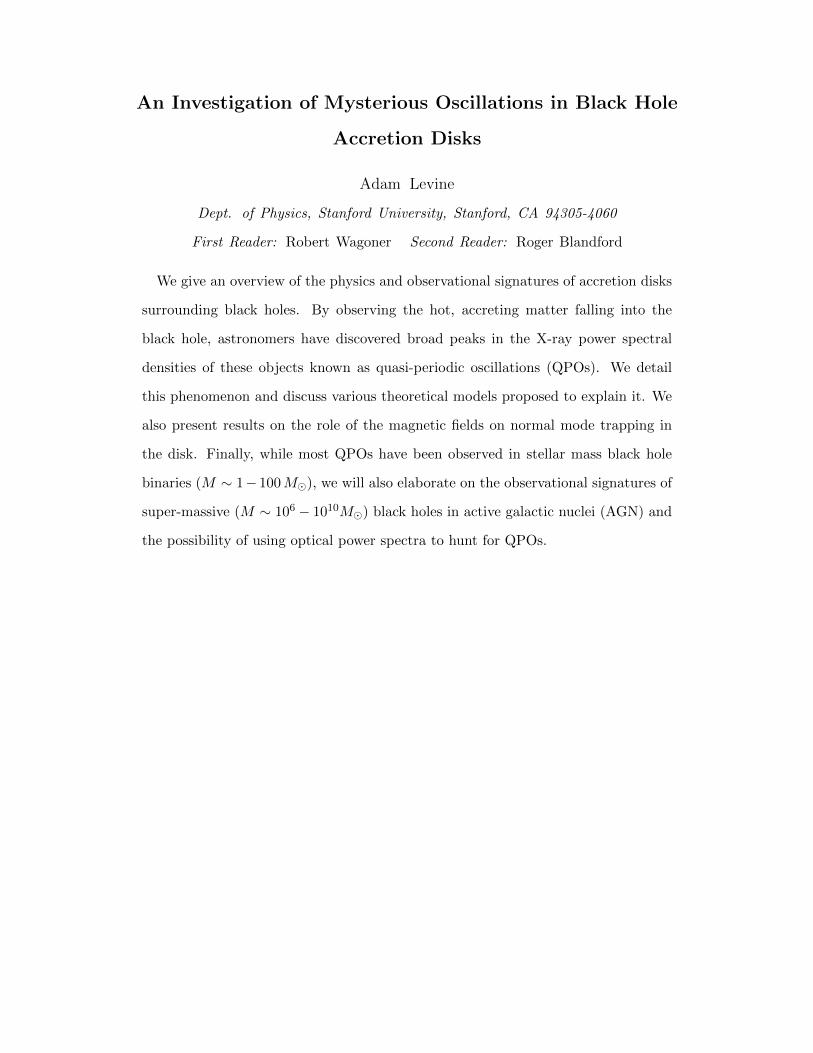
We give an overview of the physics and observational signatures of accretion disks

surrounding black holes. By observing the hot, accreting matter falling into the

black hole, astronomers have discovered broad peaks in the X-ray power spectral

densities of these objects known as quasi-periodic oscillations (QPOs). We detail

this phenomenon and discuss various theoretical models proposed to explain it. We

also present results on the role of the magnetic fields on normal mode trapping in

the disk. Finally, while most QPOs have been observed in stellar mass black hole

binaries (M ∼ 1− 100M), we will also elaborate on the observational signatures of

super-massive (M ∼ 106 − 1010M) black holes in active galactic nuclei (AGN) and

the possibility of using optical power spectra to hunt for QPOs.

2

ACKNOWLEDGEMENTS

I would like to thank the friends and family that have made this thesis possible.

My research over the past two years has been fueled by their constant support. Thank

you Mom and Dad for letting me try to explain new physics concepts over the phone

(and for being the best parents!). Thanks to Amy, Luke, Lily, Sebastian, Benjy,

Johnny, Lucio and everyone else at TDX for helping me to lighten up and take my

mind off physics (at least for a little). Thank you especially to Lucio for the espresso.

Thanks to Jack, Ikshu, Conrad, Hart and all the other physics and math majors

that have taught me almost as much as my professors. I will never forget the late

nights on the fourth floor and in XΘX. I can’t wait to go to conferences and to keep

talking about math/physics for the rest of our lives.

I would like to thank the Stanford Physics Department and the Office of Un-

dergraduate Advising and Research for supporting my research over the past two

summers. Also, thank you to Roger Blandford for agreeing to read this thesis.

Last, but most certainly not least, I must thank Bob Wagoner for being my aca-

demic guide for the past two years. His constant support and patience has been

invaluable. I would be happy with even a small fraction of his intuition about black

holes. He stuck with me through thick and thin and successfully kept me posted

on every movement of Rory McIlroy. Bob is the reason undergraduates come to a

research university: to learn from and make a lasting connection with a leader in your

field.

This thesis is dedicated to my grandfather, who passed away this summer. I will

miss his Science magazine clippings and listening to jazz with him, but will never

forget the impact he had on my interest in science.

As we begin doing physics, it is worthwhile to remember one of Bob’s favorite

sayings: “Whatever you do, don’t panic!”

3

CONTENTS

Acknowledgements 2

I. Introduction 4

II. High Frequency Quasi-Periodic Oscillations Near Black Holes 5

A. Observations 5

B. Modeling HFQPOs 7

III. Dynamics around a Kerr Black Hole 9

IV. Accretion Disk Normal Modes 10

A. Modes without Magnetic Fields 10

B. The Effect of Magnetohydrodynamics on Normal Modes 14

V. Probing the Inner Accretion Disk of AGN 19

A. Radiative Transfer in Black Hole Accretion Disks 19

B. Observation of the g-Mode in AGN 23

C. Observing with Kepler II 28

VI. Conclusion 29

References 31

4

I. INTRODUCTION

Arguably the most profound consequence of Einstein’s general theory of relativity

(GR) is the existence of mysterious objects famously known as black holes. Roughly

20 X-ray sources have been declared black hole binaries (BHBs), with an estimated

mass that rules out the presence of neutron stars or white dwarfs. A list of these

sources can be found in Remillard & McClintock (2006). In this thesis, we give an

overview of the physics and observational signatures of black hole accretion disks and

their mysterious oscillations. We will also focus on the properties of Active Galactic

Nuclei (AGN), powered by the supermassive (∼ 106 − 109M) black holes present at

galactic centers.

Via x-ray and optical observations, astrophysicists can infer properties of the cen-

tral black holes such as mass - and more recently spin. The variability in these

objects can clue the observer into the dynamics of the disk and thus gravity in a

regime where GR effects are prominent. Through computation of the power density

spectrum (PDS) of certain black hole binaries, astronomers have gained more insight

into the inner region of the disk. In particular, some spectra contain broad peaks

known as Quasi-Periodic Oscillations (QPOs) whose origin as of today remains un-

known. Some plausible explanations relate these phenomena to normal modes of the

accretion disk. If this is true, QPOs provide a clear signature of relativistic dynamics.

Theoretically, we can model the disk much like a vibrating membrane, solving

linear wave equations similar to those found in quantum mechanics. In this thesis,

we will discuss the normal modes that arise out of these equations and the orbits of

both matter and light assuming a Kerr (rotating black hole) background. We will

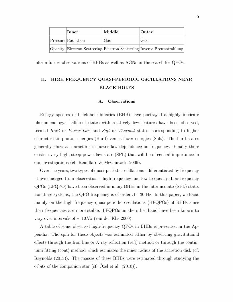
also analytically model the radiative transfer of the accretion disk. For simplicity, we

partition the disk into three distinct regions, the sizes of which depend on M . In the

following table, we list what effects dominate the local pressure and opacity in each

region. In order to accurately model the spectrum of the disk, however, we employ

numerical ray tracing using the code of Dexter & Agol (2009) to find the fraction

of photons emitted from the inner region of the disk. These calculations could help

5

Inner Middle Outer

Pressure Radiation Gas Gas

Opacity Electron Scattering Electron Scattering Inverse Bremsstrahlung

inform future observations of BHBs as well as AGNs in the search for QPOs.

II. HIGH FREQUENCY QUASI-PERIODIC OSCILLATIONS NEAR

BLACK HOLES

A. Observations

Energy spectra of black-hole binaries (BHB) have portrayed a highly intricate

phenomenology. Different states with relatively few features have been observed,

termed Hard or Power Law and Soft or Thermal states, corresponding to higher

characteristic photon energies (Hard) versus lower energies (Soft). The hard states

generally show a characteristic power law dependence on frequency. Finally there

exists a very high, steep power law state (SPL) that will be of central importance in

our investigations (cf. Remillard & McClintock, 2006).

Over the years, two types of quasi-periodic oscillations - differentiated by frequency

- have emerged from observations: high frequency and low frequency. Low frequency

QPOs (LFQPO) have been observed in many BHBs in the intermediate (SPL) state.

For these systems, the QPO frequency is of order .1 - 30 Hz. In this paper, we focus

mainly on the high frequency quasi-periodic oscillations (HFQPOs) of BHBs since

their frequencies are more stable. LFQPOs on the other hand have been known to

vary over intervals of ∼ 10Hz (van der Klis 2000).

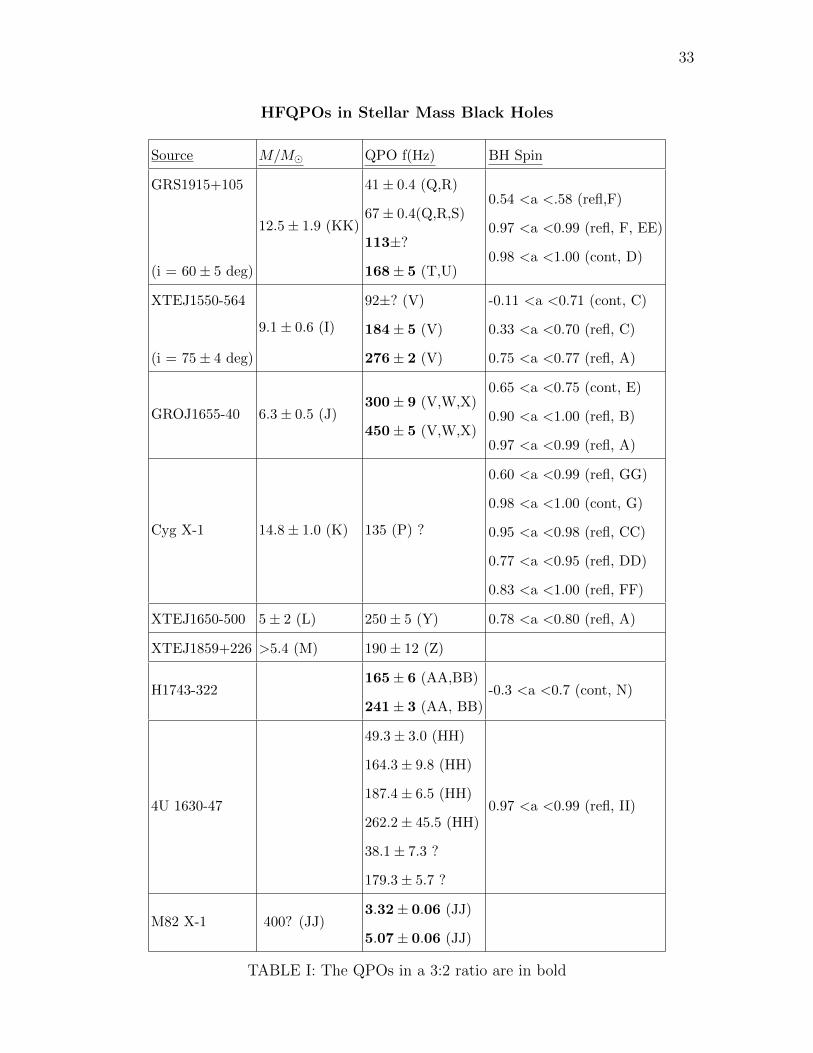
A table of some observed high-frequency QPOs in BHBs is presented in the Ap-

pendix. The spin for these objects was estimated either by observing gravitational

effects through the Iron-line or X-ray reflection (refl) method or through the contin-

uum fitting (cont) method which estimates the inner radius of the accretion disk (cf.

Reynolds (2013)). The masses of these BHBs were estimated through studying the

orbits of the companion star (cf. Ozel et al. (2010)).

6

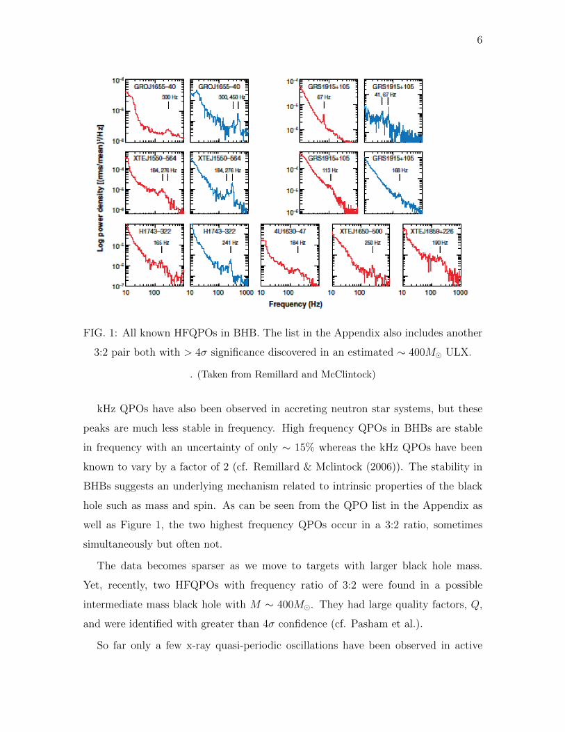
FIG. 1: All known HFQPOs in BHB. The list in the Appendix also includes another

3:2 pair both with > 4σ significance discovered in an estimated ∼ 400M ULX.

. (Taken from Remillard and McClintock)

kHz QPOs have also been observed in accreting neutron star systems, but these

peaks are much less stable in frequency. High frequency QPOs in BHBs are stable

in frequency with an uncertainty of only ∼ 15% whereas the kHz QPOs have been

known to vary by a factor of 2 (cf. Remillard & Mclintock (2006)). The stability in

BHBs suggests an underlying mechanism related to intrinsic properties of the black

hole such as mass and spin. As can be seen from the QPO list in the Appendix as

well as Figure 1, the two highest frequency QPOs occur in a 3:2 ratio, sometimes

simultaneously but often not.

The data becomes sparser as we move to targets with larger black hole mass.

Yet, recently, two HFQPOs with frequency ratio of 3:2 were found in a possible

intermediate mass black hole with M ∼ 400M. They had large quality factors, Q,

and were identified with greater than 4σ confidence (cf. Pasham et al.).

So far only a few x-ray quasi-periodic oscillations have been observed in active

7

galactic nuclei. Most observed have long time scales - as expected from naive scaling

of the period with mass - and some are most likely the analogue of LFQPOs in stellar

mass BHBs. So far no confirmed HFQPOs have been observed in AGN, although

depending on mass estimates some of the declared LFQPOs may in fact be HFQPOs.

Indeed, Alston et. al found strong evidence for a 3:2 resonance in a 4 × 106M/M

mass AGN, suggesting that this QPO falls under the heading of high frequency. The

discover of HFQPOs in AGN motivates, in part, our research and would help to

differentiate the many models proposed to explain these phenomena.

B. Modeling HFQPOs

Many explanations for high frequency quasi-periodic oscillations have been pro-

posed. Although models were originally proposed to explain QPOs observed in accret-

ing neutron stars, black holes are theoretically simpler because they do not possess

an inner surface: the accretion disk has an inner edge at the innermost stable circular

orbit (ISCO). Furthermore, high frequency QPOs tend to have periods of order the

inner orbit and so are assumed to display the dynamics of the near horizon disk.

The three most well known models are the orbiting hotspot, epicyclic resonance

and normal mode models. The first - orbiting hotspot models (cf. Schnittmann and

Bertschinger, 2003) - propose that the variations come from regions of higher relative

emission in the disk. Such a region would normally be sheared out by the differential

rotation immediately [5]. Thus, the theoretical basis for the origin of these hotspots

is unknown and so we will not focus on them in this paper.

Epicyclic resonance models were proposed (cf. Abramowicz and Kluz’niak, 2001)

to help explain the observed 3:2 ratio in QPO frequencies. These models relied on

coupling between the radial and vertical epicyclic frequencies. For horizontal and

vertical perturbations of a torus, each obeys the following relations, respectively:

d2ξrdt2

+ κ2ξr = 0

d2ξzdt2

+ Ω⊥ξz = 0 (1)

8

These equations can be coupled by replacing κ2 → κ2(1 + χ1 cos(Ω⊥t)) and Ω2⊥ →

Ω2⊥(1+χ2 cos(κt). These modified ODEs are the Mathieu equations. According to the

methods of parametric resonance, one should then see 3:2 resonances at radii where

Ω⊥(r)/κ(r) ≈ 3/2. The downside of this model arises from the fact that it does

not provide an explanation for excitation of these resonances at the specified radius.

While some work has been done regarding excitation through stochastic driving terms

in the above equations, we will not pursue these explanations further in this paper.

Finally, the focus of this paper will be on models based on oscillations of accretion

disks (diskoseismic modes). These models have many nice theoretical advantages over

the others proposed. Disk modes, as will be fleshed out in detail, are trapped at certain

radii of the disk. These modes form a complete, orthonormal set and have relatively

simple characterizations. In a rotating hydrodynamical system, as around a Kerr

black hole, a fluid element that is displaced in the radial direction will feel a restoring

force due to competition between the gravitational pull of the central object and the

centrifugal force. There will be a vertical pressure and gravitational restoring force

that will lead to oscillations. Various combinations of radial and vertical restoring

forces produce the menagerie of disk modes known as the p-, g- and c-modes. These

different types of modes will be disambiguated below.

In particular, diskoseismic modes can become trapped in the inner disk due to

a form of the radial epicyclic frequency predicted general relativity: κ has a maxi-

mum κmax at a certain radius. The fundamental g-mode can be trapped below this

maximum frequency. In our work, the axisymmetric g-mode, which agrees nicely in

frequency with those of HFQPOs, will take on frequency values of ω2 ' κ2.

A final advantage of disk oscillations is that viscous driving provides a neat mech-

anism for exciting these modes. Furthermore, they can couple non-linearly between

each other and produce a frequency ratio of 3:2 as in Horak (2008). To gain fur-

ther insight into this compelling picture, we will need to mathematically explore the

dynamics of black hole accretion disks.

It is important to note that the observed QPOs have never been seen in simulations.

This indicates that some key physical ingredient is missing from the computer models.

9

On the other hand, the fundamental g-mode, which will be discussed in depth below,

has been seen along with p-waves propagating above κmax (Reynolds & Miller (2009)).

Some (Schnittman et al. (2006)) have suggested that the missing ingredient could be

related to a proper treatment of radiative transfer in the simulations.

III. DYNAMICS AROUND A KERR BLACK HOLE

In many ways, black holes are like large fundamental particles; Kerr black holes

are parameterized by two numbers only: their spin, a = cJ/GM2, and mass, M . In

this paper, we use Boyer-Lindquist coordinates with r measured in units of M . The

Kerr metric then takes the following form:

ds2 = −r2∆

Ad t2 +

A

r2(dφ− ω dt)2 +

r2

∆d r2 + d z2 (2)

with ∆ ≡ r2 − 2r + a2, A = r4 + r2a2 + 2ra2 and ω ≡ 2ar/A. For the remainder of

this paper, we also have set G = c = 1.

With this metric in hand, we readily solve the geodesic equation, uνuµ;ν = 0, to see

that

Ω ≡ ± 1

r3/2 + a(3)

where Ω = dφdt

is the dimensionless angular velocity and the dimensionless black

hole spin a can take on values from −1 to 1. The plus or minus sign in front of Ω

corresponds to a prograde or retrograde disk respectively.

For circular orbits, we assume the coordinate velocity is just dxµ

dt= (1, 0,Ω, 0).

Perturbing these velocities, we find vr satisfies [1] for ξr where

κ = Ω(r)(1− 6/r + 8a/r3/2 − 3a2/r2)1/2 (4)

and vz satisfies [1] for ξz where

Ω⊥ = Ω(r)(1− 4a/r3/2 + 3a2/r2)1/2 (5)

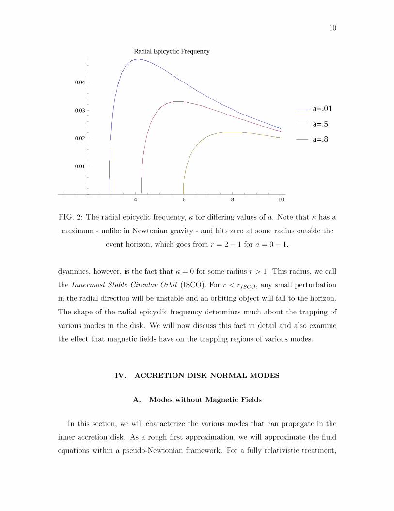
As is shown in Fig. 2, the radial epicyclic frequency has a maximum at rmax, around

which the most interesting disk oscillations are trapped. Most importantly for disk

10

4 6 8 10

0.01

0.02

0.03

0.04

Radial Epicyclic Frequency

a=.01

a=.5

a=.8

FIG. 2: The radial epicyclic frequency, κ for differing values of a. Note that κ has a

maximum - unlike in Newtonian gravity - and hits zero at some radius outside the

event horizon, which goes from r = 2− 1 for a = 0− 1.

dyanmics, however, is the fact that κ = 0 for some radius r > 1. This radius, we call

the Innermost Stable Circular Orbit (ISCO). For r < rISCO, any small perturbation

in the radial direction will be unstable and an orbiting object will fall to the horizon.

The shape of the radial epicyclic frequency determines much about the trapping of

various modes in the disk. We will now discuss this fact in detail and also examine

the effect that magnetic fields have on the trapping regions of various modes.

IV. ACCRETION DISK NORMAL MODES

A. Modes without Magnetic Fields

In this section, we will characterize the various modes that can propagate in the

inner accretion disk. As a rough first approximation, we will approximate the fluid

equations within a pseudo-Newtonian framework. For a fully relativistic treatment,

11

without use of the local WKB approximation, see Perez et al., 1997. We will follow

the basic derivation of the mode dispersion relation laid out in Fu & Lai (2008). The

main equations considered here will be the continuity equation and the momentum-

conservation equation:

∂ρ∂t

+∇ · (ρ~v) = 0 (6)

∂~v∂t

+ (v · ∇)~v = −1ρ∇Π−∇Φ + 1

ρ~T (7)

where Π is the gas and magnetic pressure of the disk, Φ is the gravitational potential

and ~T = 14π

( ~B · ∇) ~B is a magnetic stress-vector that will be needed later to describe

the effects of magnetic fields. For now, we set it to zero.

We assume a perfectly circular flow so that ~v = rΩ(r)φ and we perturb around

this solution. Following the notation of Fu & Lai (2008) and Ortega-Rodriguez et al.

(2015), the background configuration satisfies the equation

~G ≡ 1

ρ∇Π− ~T = rΩ2(r)r −∇Φ

Assuming the perturbations have the form δf ∝ eimφ−iωt, we then get the master

equations

− iωδρ+ 1r∂∂r

(ρrδvr) + imρrδvφ + ∂

∂z(ρδvz) = 0 (8)

− iωδvr − 2Ωδvφ = Grδρρ− 1

ρ∂∂rδΠ + 1

ρ(δ ~T )r (9)

− iωδvφ + κ2

2Ωδvr = − im

ρrδΠ + 1

ρ(δ ~T )φ (10)

− iωδvz = Gzδρρ− 1

ρ∂∂zδΠ + 1

ρ(δ ~T )z (11)

where the epicyclic frequency is defined as in Newtonian gravity as κ2 ≡ 2Ωrd(r2Ω)dr

and

ω ≡ ω −mΩ.

We will assume throughout this text that the disk fluid is barotropic so that

ρ = ρ(P ) and δρ = 1c2sδP . Here we have used the definition of the speed of sound as

c2s = ∂P

∂ρ. Imposing the WKB approximation, we postulate that the remaining spatial

dependence of the perturbations looks like eikrr+ikzz. Here we expand to first order in

the parameter (rkz)−1, (rkr)

−1 << 1. Plugging this ansatz into the above equations

12

and dropping negligible terms, we get

− iωρc2sδΠ + ikrδvr + ikφδvφ + ikzδvz = 0 (12)

− ikrρδΠ + iωδvr + 2Ωδvφ = 0 (13)

− ikφρ− κ2

2Ωδvr + iωδvφ = 0 (14)

− ikzρδΠ + iωδvz = 0 (15)

where kφ ≡ m/r. Furthermore, as will be done when we discuss the magneto-

hydrodynamic equations, we assume that Gz = −(∇Φ)z ∼ Ω2⊥z is negligible since

we are working near the z = 0 mid-plane. Furthermore, Gφ = 0 since we are assum-

ing an axisymmetric disk, and Gr is small since the force balance of the background

disk is assumed to be approximately Keplerian so that Ω2r ≈ (∇Φ)r.

To get the dispersion relation, we know that equations (13)-(16) define a coeffi-

cient matrix for the four unknown perturbations, δΠ, δvr, δvφ and δvz. Taking the

determinant of this matrix and setting it to zero, we get the following relation

(ω2 − κ2)(ω2 − k2zc

2s) = k2

rc2sω

2 (16)

As done more rigorously in Okazaki et al. (1987) and Nowak & Wagoner (1992), the

differential equations for the fluid perturbations can actually be separated. The ver-

tical dependence is not well described by eikzz, but, in fact, by Hermite polynomials.

Assuming an isothermal disk, the pseudo-Newtonian dispersion relation obtained in

both references is approximated by

(ω2 − κ2)(ω2 − nΩ2⊥) = k2

rc2sω

2 (17)

with n an integer. In this case, we can think of kz as quantized and write

kz ∼√nΩ⊥/cs (18)

This relation will be used below.

Equation [17] helps us to classify the various modes that propagate in the disk.

For n = 0, the modes are called fundamental p-modes. For m = 0, the dispersion

relation takes the simple form of (ω2 − κ2) = k2rc

2s. Thus, the p-mode only exists if

13

FIG. 3: Upper Left : The p-modes can propagate in the region indicated by the

green lines, where ω2 > κ2. Lower Left : The mode diagram for m > 0

non-axisymmetric p-modes. Upper Right : The mode diagram for m= 0 g-modes.

This agrees with the findings of Perez et al. (1996). The effect of magnetic fields on

these modes is discussed in the next section. Lower Right : The mode diagram for

non-axisymmetric g-modes and c-modes.

ω2 > κ2. As can be seen from the upper-left panel of Figure 3, these modes have

an important theoretically downfall; they require reflection at the ISCO in order to

remain trapped. This unlikely scenario is part of why we ignore the p-mode in the

discussion that follows.

For n = 1, the modes are called fundamental g-modes. We will consider mostly the

axisymmetric, m = 0 type. These modes satisfy the dispersion relation (ω2−κ2)(ω2−

Ω2⊥) = k2

rc2s. Thus, they can propagate in the region indicated in the upper-right

corner of Figure 3. The spectra of the g-mode was analyzed in a fully relativistic

background by Perez et al. (1996). They found the important relation that the

frequency of the fundamental g-mode obeys the equation

f(m = 0) ≈ 714(M/M)F (a) Hz (19)

where F (0) = 1 and F (.998) ≈ 3.443. This equation will be extremely important in

determining reasonable AGN targets for detailed observation. The g-mode trapping

14

FIG. 4: The mode trapping regions as a function of black hole spin. Note the

constancy of the g-mode region.

region also remains relatively stable as a function of spin as can be seen in Figure 4.

For n > 1 and m ≥ 1, the modes are called c-modes. These modes represent a pre-

cessing tilt of the inner disk. They can become trapped in the small region indicated

in the lower right panel of Figure 3. Again, they suffer from similar theoretical issues

as the p-modes. Thus, for the remainder of this thesis, we will focus our attention on

the g-mode and in particular the effect of magnetic fields on the trapping region of

Figure 3.

B. The Effect of Magnetohydrodynamics on Normal Modes

The following results were submitted to the Astrophysical Journal in Ortega-

Rodriguez et al. (2015). My contributions consisted of numerically analyzing the

effect of magnetic fields on the g-mode trapping region.

Accretion disks should contain magnetic fields accreting from the surrounding in-

terstellar medium. The study of magnetized fluids or magnetohydrodynamics (MHD)

15

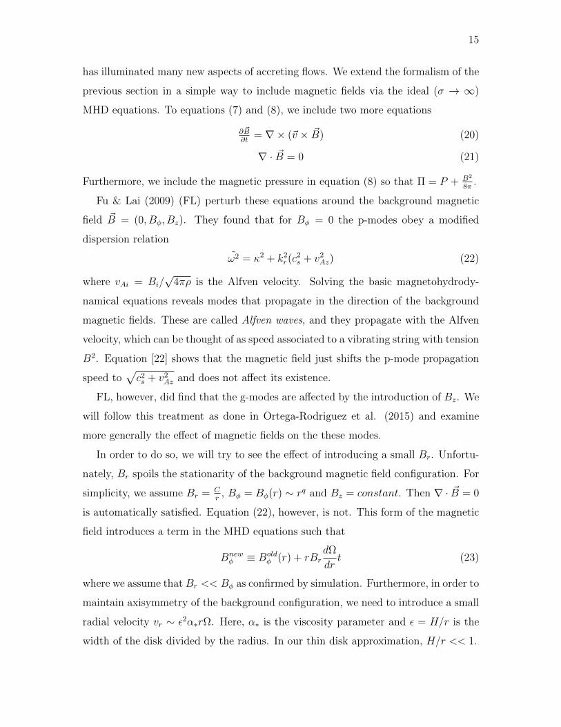
has illuminated many new aspects of accreting flows. We extend the formalism of the

previous section in a simple way to include magnetic fields via the ideal (σ → ∞)

MHD equations. To equations (7) and (8), we include two more equations

∂ ~B∂t

= ∇× (~v × ~B) (20)

∇ · ~B = 0 (21)

Furthermore, we include the magnetic pressure in equation (8) so that Π = P + B2

8π.

Fu & Lai (2009) (FL) perturb these equations around the background magnetic

field ~B = (0, Bφ, Bz). They found that for Bφ = 0 the p-modes obey a modified

dispersion relation

ω2 = κ2 + k2r(c

2s + v2

Az) (22)

where vAi = Bi/√

4πρ is the Alfven velocity. Solving the basic magnetohydrody-

namical equations reveals modes that propagate in the direction of the background

magnetic fields. These are called Alfven waves, and they propagate with the Alfven

velocity, which can be thought of as speed associated to a vibrating string with tension

B2. Equation [22] shows that the magnetic field just shifts the p-mode propagation

speed to√c2s + v2

Az and does not affect its existence.

FL, however, did find that the g-modes are affected by the introduction of Bz. We

will follow this treatment as done in Ortega-Rodriguez et al. (2015) and examine

more generally the effect of magnetic fields on the these modes.

In order to do so, we will try to see the effect of introducing a small Br. Unfortu-

nately, Br spoils the stationarity of the background magnetic field configuration. For

simplicity, we assume Br = Cr

, Bφ = Bφ(r) ∼ rq and Bz = constant. Then ∇ · ~B = 0

is automatically satisfied. Equation (22), however, is not. This form of the magnetic

field introduces a term in the MHD equations such that

Bnewφ ≡ Bold

φ (r) + rBrdΩ

drt (23)

where we assume that Br << Bφ as confirmed by simulation. Furthermore, in order to

maintain axisymmetry of the background configuration, we need to introduce a small

radial velocity vr ∼ ε2α∗rΩ. Here, α∗ is the viscosity parameter and ε = H/r is the

width of the disk divided by the radius. In our thin disk approximation, H/r << 1.

16

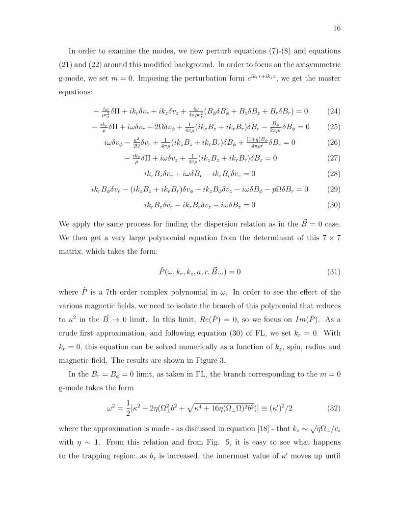
In order to examine the modes, we now perturb equations (7)-(8) and equations

(21) and (22) around this modified background. In order to focus on the axisymmetric

g-mode, we set m = 0. Imposing the perturbation form eikrr+ikzz, we get the master

equations:

− iωρc2sδΠ + ikrδvr + ikzδvz + iω

4πρc2s(BφδBφ +BzδBz +BrδBr) = 0 (24)

− ikrρδΠ + iωδvr + 2Ωδvφ + 1

4πρ(ikzBz + ikrBr)δBr − Bφ

2πρrδBφ = 0 (25)

iωδvφ − κ2

2Ωδvr + 1

4πρ(ikzBz + ikrBr)δBφ +

(1+q)Bφ4πρr

δBr = 0 (26)

− ikzρδΠ + iωδvz + 1

4πρ(ikzBz + ikrBr)δBz = 0 (27)

ikzBzδvr + iωδBr − ikzBrδvz = 0 (28)

ikrBφδvr − (ikzBz + ikrBr)δvφ + ikzBφδvz − iωδBφ − pΩδBr = 0 (29)

ikrBzδvr − ikrBrδvz − iωδBz = 0 (30)

We apply the same process for finding the dispersion relation as in the ~B = 0 case.

We then get a very large polynomial equation from the determinant of this 7 × 7

matrix, which takes the form:

P (ω, kr, kz, a, r, ~B...) = 0 (31)

where P is a 7th order complex polynomial in ω. In order to see the effect of the

various magnetic fields, we need to isolate the branch of this polynomial that reduces

to κ2 in the ~B → 0 limit. In this limit, Re(P ) = 0, so we focus on Im(P ). As a

crude first approximation, and following equation (30) of FL, we set kr = 0. With

kr = 0, this equation can be solved numerically as a function of kz, spin, radius and

magnetic field. The results are shown in Figure 3.

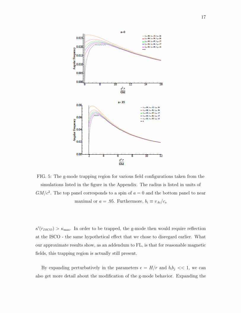
In the Br = Bφ = 0 limit, as taken in FL, the branch corresponding to the m = 0

g-mode takes the form

ω2 =1

2[κ2 + 2η(Ω2

⊥b2 +

√κ4 + 16η(Ω⊥Ω)2b2)] ≡ (κ′)2/2 (32)

where the approximation is made - as discussed in equation [18] - that kz ∼√ηΩ⊥/cs

with η ∼ 1. From this relation and from Fig. 5, it is easy to see what happens

to the trapping region: as bz is increased, the innermost value of κ′ moves up until

17

FIG. 5: The g-mode trapping region for various field configurations taken from the

simulations listed in the figure in the Appendix. The radius is listed in units of

GM/c2. The top panel corresponds to a spin of a = 0 and the bottom panel to near

maximal or a = .95. Furthermore, bi ≡ vAi/cs

κ′(rISCO) > κmax. In order to be trapped, the g-mode then would require reflection

at the ISCO - the same hypothetical effect that we chose to disregard earlier. What

our approximate results show, as an addendum to FL, is that for reasonable magnetic

fields, this trapping region is actually still present.

By expanding perturbatively in the parameters ε = H/r and bibj << 1, we can

also get more detail about the modification of the g-mode behavior. Expanding the

18

branch frequency as

ω = ω0 + Λbφbz + λbφbr + Γb2z + γb2

r + βbzbr (33)

we find order by order that each coefficient has a real and imaginary part. This

suggests some instability in this mode. Interestingly, the leading order imaginary

term comes from the bzbφ term, explaining why FL did not find it. The imaginary

contribution to this term is

Im(Λ) =kzkrc

2s[2(2 + p)Ω2 − κ2]

4Ω(k2zc

2s − κ2)

(34)

Interestingly, for Newtonian mechanics, where κ2 = 2Ωrd(r2Ω)dr

, Im(Λ) = 0 and so this

instability (or damping) is purely relativistic. The effects of it are minimal as they are

suppressed by order ε1/2, but more work investigating the potential for this imaginary

term as a mode excitation mechanism or otherwise is needed.

Finally, we note that the g-mode appears to be safe from the famous magneto-

rotational instability (MRI) of Balbus & Hawley (1998). We found perturbatively

that the timescale of the g-mode, τg, can be related to the MRI timescale, τMRI by

the relationτg

τMRI

∼ Ωb1/2z

κ(35)

This relation allows roughly 3 g-mode oscillations for typical bz values as listed in

the Appendix. This means that the g-mode will oscillate a few times before being

destroyed by MRI (cf. Ortega-Rodriguez et al. (2015)).

In summary, we find no reason to discard the g-mode based upon destruction of

the κ trapping effect, as FL suggested in their work. For the magnetic fields listed in

the Appendix, and those used to generate Fig. 5, the g-mode trapping region remains

intact. Furthermore, the magnetic field needs to only take on acceptable values for

relatively short amounts of time since QPO duty cycles are quite small (Rodriguez et

al. (2015)).

These results were focused more on QPOs observed in stellar mass black hole bina-

ries. With few new X-ray telescopes launching in the next decade, optical telescopes

may provide a new avenue to observe black hole accretion disks. Since the tempera-

ture of the disk scales inversely with the mass, as will be discussed in the next section,

19

the plausibility of observing the inner disk with optical telescopes is higher for targets

with large masses. We now explore the possibility of using super-massive black holes

that power active galactic nuclei (AGN) to continue the hunt for QPOs and other

strong-gravity phenomena.

V. PROBING THE INNER ACCRETION DISK OF AGN

We now discuss using observations of AGN to access the inner accretion disk

via lower energy spectra. This could increase the number of targets with observed

QPOs and give us more observational evidence for the scalings of basic properties of

this phenomena as a function of mass. We examine the properties of AGN spectra

in order to inform a selection of adequate targets. We have submitted a proposal

for observation of selected targets in the Kepler II mission. The advantages and

disadvantages of this particular search will be discussed below. The use of data from

LSST will also be considered.

A. Radiative Transfer in Black Hole Accretion Disks

We begin by studying the basics of accretion around black holes and how modes

will modulate observable properties of this disk. Following the treatment in Shapiro

and Teukolsky (1983), we note that the main energy generation mechanism occurs

from viscous stresses slowing down and heating up the in-falling gas. The hottest

part of the disk will occur near the inner edge of the disk. The main mechanism of

accretion will occur through angular momentum transfer to larger radii with mass

transfer inward. Quantitatively, we can see this phenomenon in the approximation

of a Keplerian disk around a black hole. For illustration purposes, we will derive the

luminosity of a black hole accretion disk in Newtonian gravity.

First, we assume as in the previous section that, H(r) << r. Thus we will integrate

out any dependence on z. In this spirit, we define

Σ =

∫ H

−Hρd z ≈ ρ2H (36)

20

is the surface density of the disk. We also assume that vφ = rΩ = (GMr

)1/2. Using the

Navier-Stokes equations in combination with force balance, we find that the azimuthal

stress due to two radially separated fluid elements (r → r + dr) is just

fφ = −trφ = −3

2η

(GM

r3

)1/2

(37)

Here η = αρHcs is the dynamic viscosity. The viscosity parameter α <∼ 1 appears in

the disk equations discussed below.

Then the angular momentum transport inward across a cylinder of radius r and

heigh 2h will just be J+ = M√GMr where

√GMr is just the specific angular

momentum of a fluid element at radius r and M is the mass accretion rate of the

central black hole. The amount of angular momentum swallowed by the black hole

is just βM√GMrISCO, with β ≤ 1, and so, by angular momentum conservation, we

find that the total angular momentum added to the section of the disk between rISCO

and r is just

trφ · 2πr · 2h = M[β√GMrISCO −

√GMr

](38)

Note, trφ < 0 indicating that angular momentum is being carried out to larger radii.

Then the basic equations of energy transport in a fluid state that the heat (or

entropy by the Second Law of Thermodynamics) are given by the square of the stress

tensor. Thus,

Q = ρT s ≈t2rφη

= −fφtrφη

(39)

Assuming this heat is totally radiated away, the flux per unit area of heat energy is

then just F (r) = 1/2× 2HQ. The 1/2 is for each side of the disk, and the 2H comes

from integrating out the z-dependence. Thus, using [37] and [38], we get

F (r) =3M

8πr2

GM

r

[1− β

(rISCOr

)1/2]

(40)

Integrating over r to get the total disk luminosity, we finally get

L =

∫ ∞rISCO

2F × 2πrd r =

(3

2− β

)GMM

rISCO(41)

This final equation is how we estimate accretion rate and mass of the central black

hole of AGN. While it is not relativistic, it provides many heuristics for the radiation

properties of black hole accretion disks.

21

In our work, we also took into account the effects of opacity and radiative transfer,

which simulations so far have not been able to do successfully. Proper radiative trans-

fer prevents disks from puffing up into their thick, radiatively inefficient counterpart.

In order to include these effects, we must discuss the overall structure of an accretion

disk.

As discussed in the introduction, there are three regions of the disk: outer, middle

and inner. In the outer region, gas pressure dominates radiation pressure. Further-

more, free-free (e− → e−) absorption contributes most significantly to the opacity.

The middle-outer transition occurs when the contribution to the total opacity from

free-free absorption is roughly that from electron scattering (e− + γ → e− + γ) or

κff ≈ κes. Finally the middle - inner transition occurs where the radiation pressure

and gas pressure are comparable or where Pgas ∼ Prad.

In order to assess the effects of opacity on the emergent disk spectrum, we first

need to clear up some terminology regarding what temperature we are actually cal-

culating. In 1973, Shakura & Sunyaev solved for the disk temperature T involved in

the radiative transport equation. They found that, for the inner region of the disk,

T = (5× 107K)(αM)−1/4(2r)−3/8 (42)

with r in units of M , M in units of M and α <∼ 1 is the viscosity parameter mentioned

above. This T corresponds to the temperature at the midplane of the disk. We can

also define a surface temperature Ts. For optically thick regions of the disk, the

surface temperature will be roughly the same as the effective blackbody temperature

Teff =(

4F (r)a

)1/4

. Using equation [40] that we derived above, we can solve for this

temperature as a function of radius.

This approximation will only hold, however, when free-free absorption dominates

the disk opacity. In the inner and middle disk, where κff <∼ κes, we have to take

into account that photons in the disk zig-zag before arriving at the surface; they

originate at larger z values than in the outer disk. Since fewer photons will arrive

at the surface, the emitted photons will have higher characteristic frequency so as to

radiate the same total energy as for a black-body spectrum. We expect then that this

modified black-body spectrum will be skewed toward higher photon energies.

22

Quantitatively the modified black-body spectrum can be modeled by the equation

Iν ∼ Bν(Ts)

(κffνκes

)1/2

(43)

A detailed derivation of this modification can be found in Shapiro & Teukolsky (1983).

Equation [43] will be essential for our results.

Using the formulae derived in Novikov & Thorne (1973) for

κffν ∼ (1.5× 1025cm2g−1)ρT−7/2gff1− e−x

x3(44)

and the well-known value of κes ∼ .40cm2g−1 from Thomson scattering calculations,

we can explicitly write down an expression for Iν using (43). Integrating over the

upper half-sphere and over frequency, we find an expression for F :

F =∫ π/2

0

∫∞0Iν cos θdΩ dν

∼ C 2.54×10−3kBh

ρ1/2T9/4s [erg/cm2/s] (45)

where C =∫∞

0x3/2e−x/2√

ex−1. This is the modified black-body analogue of the famous

relation F ∼ T 4. The use of equation (45), (40) and the relation for ρ found in

Novikov and Thorne then allows us to solve for Ts(r). For the inner region, we find

that the temperature is

Ts = 8.47× 1018 · L/(M · η · r3) · ρ−1/2 · Q(r, a)/(B(r, a) ·√C(r, a))4/9[K] (46)

where Q,B and C are given in Novikov & Thorne (1973), M is in units of M and r

is in units of GM/c2.

The temperature of the disk as a function of the radial coordinate can be seen in

Fig. 6. Equation (46) can then be plugged back into (45) and integrated over r to

find an expression for Lν and L respectively. With these equations in hand, we can

investigate how the observational properties of the g-Mode change with varying spin,

mass, luminosity and inclination angle of a target AGN. We take up this subject in

the next section.

23

5 10 15 20r @MD

5´104

1´105

2´105

5´105

Ts @KDa = .8M, L=.3 LEdd

FIG. 6: The temperature of an accretion disk with central object mass of 109M,

luminosity L ∼ .3LEdd and spin a = .8. Note that the maximum occurs near the

maximum of κ (r = blahblahblah PUT THIS IN) and so g-modes are modulating a

region of high output flux. For this reason, the g-mode should be more likely

observable.

B. Observation of the g-Mode in AGN

Since the g-mode should occupy the region near the hottest part of the disk -

as can be seen from comparison of Fig. 4 and 6 - they should be the most easily

observable candidate mode. In this section, then, we focus on what exactly should

be observed in AGN with a characteristic g-mode. We will follow and expand upon

the treatment given in Nowak & Wagoner 1993. Most of the following work was done

with the intention of using the upcoming Large Synoptic Survey Telescope (LSST)

to monitor AGN in optical bands. We will then use band widths specific to LSST,

but the results can be easily generalized to any other search.

In order to estimate the effect of the mode on the object luminosity, we need to

first find how the fractional luminosity varies with spin. Assuming that the fractional

modulation at radius r of the g-mode is given by fg(r), we can find the fractional

modulation by integrating:

δLν/Lν =

∫ ∞r=rISCO

fg(r)Fν′(r)2πr dr/

∫ ∞r=rISCO

Fν′(r)2πr dr (47)

where ν ′ is the frequency of light at observer. For our work, we were interested mostly

24

in scaling of these observational signatures and so set fg(r) to be a step function

comprising the mode region. As indicated in Fig. 4, we set boundaries of this step

function to [1.3rISCO, 1.3rISCO + 2].

The problem with trying to extract information from optical power spectra comes

from the fact that the characteristic photon frequency of the g-mode region is ν ∼

1015Hz, which lies well into the UV. In order to compensate for this, we focused on

AGN candidates whose redshift was large enough to move the Lyman limit to the low

frequency end of the LSST u-band. This corresponds to a redshift of z ∼ 3.42.

The work of Nowak & Wagoner was done non-relativistically and did not account

for the effects of gravitational redshift and doppler shifts. Per the discussion of the

previous paragraph, the gravitational redshift could actually help bring the higher

energy photons of the inner disk into the observation band. Yet, as we increase a,

the disk will be pulled in closer to the event horizon, increasing the characteristic

temperature of the disk. A priori, we do not know which effect will dominate if any.

We carried out an expanded analysis to examine this interplay. The frequency shift

of a photon originating near a Kerr black hole is

ν0

ν∞=

r3/2 + a+ b sinα cosϕ

r3/4(r3/2 − 3r1/2 + 2a)1/2(48)

where b is the impact parameter at which the photon crosses the observers image plane

at infinity, ϕ is the angular coordinate in the image plane and α is the inclination

angle of the disk. Furthermore, we accounted for the angular dependence of a rotating,

scattering dominated atmosphere given in (Perez, 1993). This gives

Iν0 =2π

c2MBF (r)

as + bsγ

2π(as2

+ bs2

)(49)

where as ≈ 0.36 and bs ≈ 0.64 as found by (Perez, 1993) through numerical fitting to

theoretical results in (Schneider & Wagoner, 1987). MBF is the modified blackbody

function as discussed above. Here also we have included the cosine, γ, of the angle of

the emergent photon with respect to the disk normal. The relativistic generalization

25

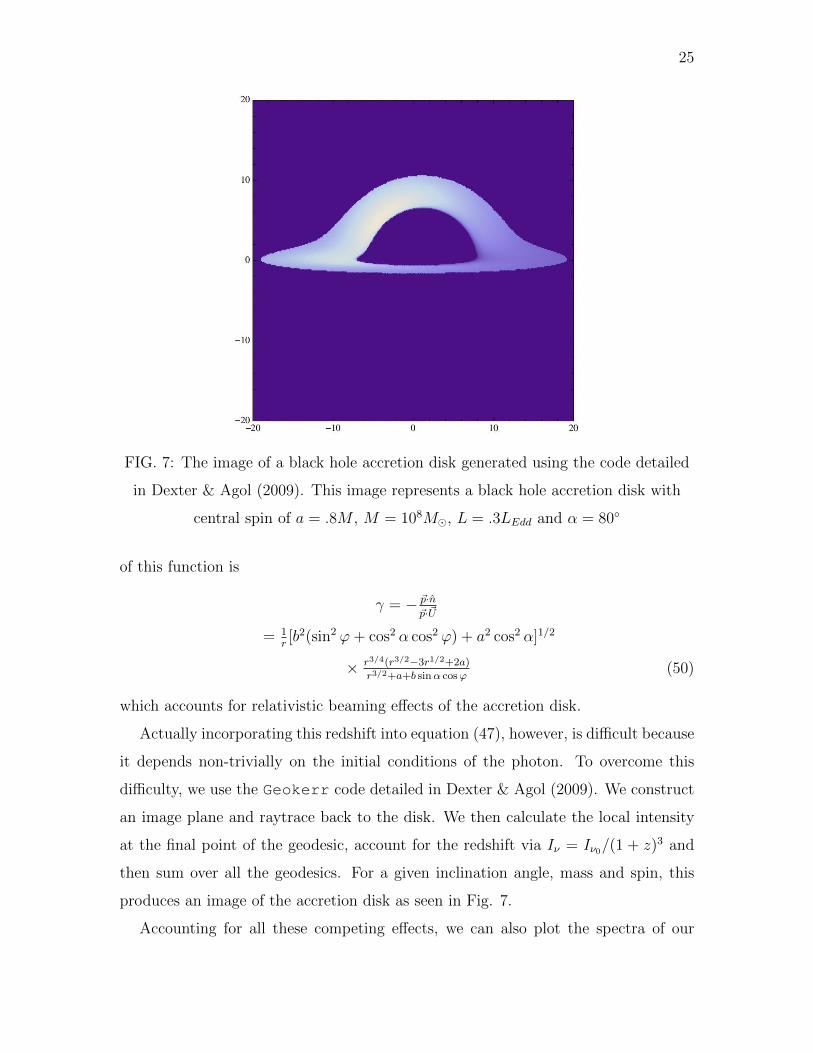
FIG. 7: The image of a black hole accretion disk generated using the code detailed

in Dexter & Agol (2009). This image represents a black hole accretion disk with

central spin of a = .8M , M = 108M, L = .3LEdd and α = 80

of this function is

γ = − ~p·n~p·~U

= 1r[b2(sin2 ϕ+ cos2 α cos2 ϕ) + a2 cos2 α]1/2

× r3/4(r3/2−3r1/2+2a)

r3/2+a+b sinα cosϕ(50)

which accounts for relativistic beaming effects of the accretion disk.

Actually incorporating this redshift into equation (47), however, is difficult because

it depends non-trivially on the initial conditions of the photon. To overcome this

difficulty, we use the Geokerr code detailed in Dexter & Agol (2009). We construct

an image plane and raytrace back to the disk. We then calculate the local intensity

at the final point of the geodesic, account for the redshift via Iν = Iν0/(1 + z)3 and

then sum over all the geodesics. For a given inclination angle, mass and spin, this

produces an image of the accretion disk as seen in Fig. 7.

Accounting for all these competing effects, we can also plot the spectra of our

26

ò

ò

ò

ò

ò

ò

òò

òò ò ò ò ò ò ò ò ò

ò

ò

ò

ò

ò

ò

à

à

à

à

à

à

à

àà à

à

à

à

à

à

Lyman

Limit

G-Band

14 15 16 17 18 19

Log10

Ν

36

38

40

42

44

Log10

HΝdLΝ

dW

L

L=.3LEdd,M=108M, i=30°

ò a=.98

à a=.20

(a) The spectrum for an M = 108M,

L = .3LEdd and α = 30 accretion disk

with two differing spins (a=.98 on top

and a=.20 on bottom). Note the

modified black body behavior where the

a = 0.98 spectrum takes the form of νp

for ν ∼ 1015.5 − 1017.5. Our estimation

puts p ≈ 1/6.

ò

ò

ò

ò

ò

ò

òò

ò ò ò ò ò òò

ò

ò

ò

ò

ò

òò

à

à

à

à

à

à

à

àà

àà

àà à à

à

à

à

à

à

Lyman Limit

G-Band

15 16 17 18

Log10

Ν

34

36

38

40

42

44

Log10

HΝdLΝ

dW

L

L=.3LEdd,M=108M, a=.8

ò i = 0°

à i = 85°

(b) The spectrum for an M = 108M,

L = .3LEdd and a = .8M accretion disk

with differing inclination angles of

α = 0 on top and α = 85 on bottom.

Note the effect of inclination angle.

Higher inclination angles will contribute

more relativistically-beamed photons to

the spectrum.

FIG. 8: Accretion disk spectra accounting for gravitatoinal redshift

accretion disk for differing inclination angles and spins as in Fig. 6. The effect of

spin is obvious; the accretion disk is pulled in closer to the horizon and so increases

in temperature. The flux thus increases overall and gets harder contributions from

emergent disk photons. Note that inclination angle appears to have a much smaller

effect on the spectrum than spin of the black hole. We are now in a tricky position.

In order to optimize flux from the g-mode region (inner disk), we should be observing

high spin AGN. Conversely, this will pull more intensity out of the optical bands and

into the UV. Thus, we need to examine more closely how the fractional modulation

looks for various disk parameters.

Indeed, we find a very interesting result, that Nowak & Wagoner (1993) did not

find in their work. As can be see from Fig. 9, the fractional modulation due to the g-

mode appears to minimize at a given mass of roughly M ∼ 107M. Interestingly, very

small mass AGN (105M) at a high inclination angle are about as good a candidate

as high mass AGN (109M).

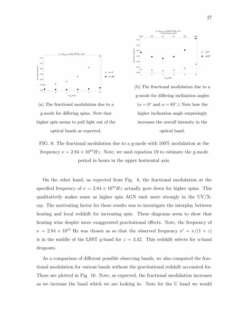
27

òò

ò

ò

ò

ò

à à à à àà

5 6 7 8 9 10

0.00

0.02

0.04

0.06

0.08

0.10

0.12

Log10

MM

Fra

cti

onalL

um

inosi

ty

L=.3LEdd, Ν=2.84*1015

Hz, i=30°

ò a=.2

à a=.98

(a) The fractional modulation due to a

g-mode for differing spins. Note that

higher spin seems to pull light out of the

optical bands as expected.

òò ò ò

ò

ò

à

à

à

à

à

à

5 6 7 8 9 10

0.00

0.02

0.04

0.06

0.08

0.10

0.12

0.085 0.85 8.5 85 850 8500

Log10

MM

Fra

cti

onalL

um

inosi

ty

G-Mode Period in Hours

L=.3LEdd, Ν=2.84*1015

Hz, a=.8

ò i=0°

à i=85°

(b) The fractional modulation due to a

g-mode for differing inclination angles

(α = 0 and α = 85.) Note how the

higher inclination angle surprisingly

increases the overall intensity in the

optical band.

FIG. 9: The fractional modulation due to a g-mode with 100% modulation at the

frequency ν = 2.84× 1015Hz. Note, we used equation 19 to estimate the g-mode

period in hours in the upper horizontal axis.

On the other hand, as expected from Fig. 8, the fractional modulation at the

specified frequency of ν = 2.84 × 1015Hz actually goes down for higher spins. This

qualitatively makes sense as higher spin AGN emit more strongly in the UV/X-

ray. The motivating factor for these results was to investigate the interplay between

heating and local redshift for increasing spin. These diagrams seem to show that

heating wins despite more exaggerated gravitational effects. Note, the frequency of

ν = 2.84 × 1015 Hz was chosen as so that the observed frequency ν ′ = ν/(1 + z)

is in the middle of the LSST g-band for z = 3.42. This redshift selects for u-band

dropouts.

As a comparison of different possible observing bands, we also computed the frac-

tional modulation for various bands without the gravitational redshift accounted for.

These are plotted in Fig. 10. Note, as expected, the fractional modulation increases

as we increase the band which we are looking in. Note for the U band we would

28

ææ

æ

æ

8.0 ´10141.0 ´1015 1.2 ´1015 1.4 ´1015 1.6 ´1015

Ν @HzD0.011

0.012

0.013

0.014

0.015

0.016

∆LΝLΝ

FIG. 10: The fractional modulation in different bands. The horizontal axis

corresponds to the middle frequency of the band; I band (leftmost), R band

(left-middle), G band (right-middle), U band (rightmost). This plot corresponds to

a black hole with spin a = .8M , L = .3LEdd and M = 108M and z = 3.42

need to look for ∼ 1.6% modulations in the light curve. Indeed, we explore the ob-

servational viability of using power spectra of AGN as a tool for studying the inner

accretion disk. This resulted in a proposal sent to NASA for their Kepler II mission

as described in the following section.

C. Observing with Kepler II

Although originally designed with the intent of finding exoplanets (planets out-

side our own solar system), the loss of a gyroscope has forced NASA to repurpose

the Kepler satellite telescope. What follows is taken from a proposal to NASA to

participate in Kepler II (K2) Campaign 6.

Campaign 6 will be optimal for extragalactic observation. The above calculations

were used to estimate the best candidates. Indeed, the QPO period for an AGN is

estimated to be

P = CP (1 + z)(M/107M)hours (51)

where z is the cosmological redshift and CP is a numerical factor that ranges from

1.1 for a = M to 4.0 for a = 0. K2 will have a maximum cadence of 30 minutes and

29

duration of 80 days. Using equation (51), we know that the AGN mass - and thus

luminosity via the Eddington relation - will range from

1.7× 1011L << (CP/CL)(1 + z)L << 7× 1014L (52)

with CL = L/LEdd < 1. We then used the redshift-magnitude relation for an FRW

universe

mi = Ai − 2.5 log(L/L)− 2.5 log(Qi(z)) + 5 log(D(z)) (53)

for a given band i. Ai here is a constant, D(z) is the luminosity distance and Qi(z) is

the luminosity emitted into the observed band divided by the total luminosity. With

our calculations above, Qi(z) was calculated for a characteristic mass of M ∼ 108M

and a = .8M . The redshifts were only allowed to be in the range 0.7 < z < 2.9

to avoid both the Lyman-α forest as well as contamination from the host galaxy.

STEM students from the high school Phillips Academy then used mi and z values

from the Million Quasar (MILLIQUAS) catalog to compute estimates on L and thus

M . Luminosities outside of the above range were rejected. A list of these targets is

presented in the Appendix.

Note that even if this search does not produce any QPOs, useful information can

be obtained from the PSDs. Break frequencies where the power-law slope changes

discontinuously at some characteristic frequency or the slope values themselves can

contribute to a deeper understanding of the dynamics around the central object.

VI. CONCLUSION

In summary, we have discussed the effect magnetic fields have on normal mode

trapping in a black hole accretion disk. We showed that, despite the claims of Fu &

Lai (2009), the g-mode trapping region is relatively stable under the magnetic field

configurations indicated by simulations. Furthermore, we showed that the vertical

and azimuthal magnetic field couple to give a purely general relativistic instability.

Although this instability arises at higher order in perturbation theory, its existence

indicates the need for further examination of basic MHD in accretion disks.

30

We have also expanded on the work of Nowak & Wagoner (1992) in including the

effects of gravitational redshift and relativistic Doppler shift. In order to provide

a full treatment, we used the code of Dexter & Agol (2009) to raytrace from the

image plane. We found interesting behavior in the fractional luminosity due to g-

mode modulation. In particular, competing effects due to decreased temperature but

increased overall luminosity seem to create a mass of minimum fractional modulation

at M ∼ 107M. We also found that the spectrum could be well approximated by

ν dLνdΩ∼ ν0.6. This calculation allowed us to compute Qi(z) and compile a target list

of AGN. We proposed this list for Kepler 2 Campaign 6.

We now await observation time with K2. If awarded guest observer status, we will

begin data analysis this Fall after data collection over the Summer. In the future, we

would like to take this work in two other directions:

• Investigate the use of the deep drilling LSST fields to obtain more optical power

spectra of AGN. The relative dearth of high cadence X-ray telescopes launching

within the next 10 years has required different techniques for finding QPOs.

LSST has a maximum cadence similar to that of K2. This requires creating a

metric to evaluate the large scale simulations of future LSST runs. Our metric

will detail the feasibility of using LSST to monitor AGN for observing QPOs.

• Explore the effect of turbulent driving of modes and the coupling between modes

and turbulence. This could include a detailed analysis of the instability discov-

ered in our investigations of magnetic disk modes.

• Finally, we hope to further characterize the various dependencies of accretion

disk spectral features on black hole mass, luminosity and spin. This would

aid observers in understanding and identifying the signatures of accretion disk

dynamics.

This work was supported through the Stanford Physics Department as well as

through an Undergraduate Advising and Research Grant.

31

[1] Alston et al., 2015, MNRAS, 449, 467.

[2] Balbus, S. and J. Hawley, 1998, Rev. Mod. Phys., 70, 1.

[3] Bardeen et al., 1972, ApJ, 178, 347.

[4] Belloni, T. and L. Stella, 2014, arXiv:1407.7373v1.

[5] Blandford, Roger. In conversation, 25, May, 2015.

[6] Dexter, J. and E. Agol, 2009, 696, 1616.

[7] Fu, W. and Dong Lai, 2009, ApJ, 690, 1386.

[8] Horak, J., 2008, A&A, 486,1.

[9] Kato, S., Fukue, J., & Mineshige, S. (1998). Black-hole accretion disks. Kyoto, Japan:

Kyoto University Press.

[10] Lehr et al., arXiv:astro-ph/0004211.

[11] Lin et al., 2013, arXiv:1309.4440v2.

[12] Mohan, P. and A. Mangalam, 2014, ApJ, 791, 74.

[13] I.D. Novikov and K.S. Thorne, ”Astrophysics of Black Holes,” in Black Holes, eds. C.

DeWitt and B. DeWitt (Gordon and Breach, Paris, 1973), pp. 343-450

[14] Nowak, M. and R. Wagoner, 1991, ApJ, 378, 656.

[15] Nowak, M. and R. Wagoner, 1993, ApJ, 418, 187.

[16] Okazaki et al., 1986, Pub. Astron. Soc. Japan, 39, 457.

[17] Ortega-Rodriguez, 2014, 440, 3011.

[18] Ortega-Rodriguez et al., 2015, submitted to ApJ.

[19] Ozel et al., 2010, ApJ, 725, 1918.

[20] Pasham et al., 2014, Nature, 74, 514.

[21] Perez, C.A., 1993, Ph.D. Thesis, Stanford University

[22] Perez et al., 1996, 476, 589.

[23] Remillard, R. and J. McClintock, 2006, Annu. Rev. Astron. Astrophys., 44, 49.

[24] Reynolds, C. and M. Miller, 2008, ApJ, 692, 869.

[25] Reynolds, C. S. 2014, Space Sci. Rev., 183, 277.

32

[26] Shapiro, S. L, & Teukolsky, S. A. (1983). Black holes, white dwarfs, and neutron stars

: the physics of compact objects. New York: Wiley.

[27] Silbergleit et al., 2000, arXiv:astro-ph/0004114.

[28] Wagoner et al., 2015, “Proposal to Kepler 2.”

[29] Wagoner, 2008, New Astron. Rev., 51, 828.

[30] Schnittman, J. and E. Bertschinger, 2003, arXiv:astro-ph/0312406.

[31] Schnittman, J. et al., 2006, ApJ, 651, 1031.

[32] Shu, F. H. (1991). The physics of astrophysics. Mill Valley, Calif.: University Science

Books.

[33] Wagoner, 2012, ApJ, 752, L18.

33

HFQPOs in Stellar Mass Black Holes

Source M/M QPO f(Hz) BH Spin

GRS1915+105

(i = 60± 5 deg)

12.5± 1.9 (KK)

41± 0.4 (Q,R)

67± 0.4(Q,R,S)

113±?

168± 5 (T,U)

0.54 <a <.58 (refl,F)

0.97 <a <0.99 (refl, F, EE)

0.98 <a <1.00 (cont, D)

XTEJ1550-564

(i = 75± 4 deg)

9.1± 0.6 (I)

92±? (V)

184± 5 (V)

276± 2 (V)

-0.11 <a <0.71 (cont, C)

0.33 <a <0.70 (refl, C)

0.75 <a <0.77 (refl, A)

GROJ1655-40 6.3± 0.5 (J)300± 9 (V,W,X)

450± 5 (V,W,X)

0.65 <a <0.75 (cont, E)

0.90 <a <1.00 (refl, B)

0.97 <a <0.99 (refl, A)

Cyg X-1 14.8± 1.0 (K) 135 (P) ?

0.60 <a <0.99 (refl, GG)

0.98 <a <1.00 (cont, G)

0.95 <a <0.98 (refl, CC)

0.77 <a <0.95 (refl, DD)

0.83 <a <1.00 (refl, FF)

XTEJ1650-500 5± 2 (L) 250± 5 (Y) 0.78 <a <0.80 (refl, A)

XTEJ1859+226 >5.4 (M) 190± 12 (Z)

H1743-322165± 6 (AA,BB)

241± 3 (AA, BB)-0.3 <a <0.7 (cont, N)

4U 1630-47

49.3± 3.0 (HH)

164.3± 9.8 (HH)

187.4± 6.5 (HH)

262.2± 45.5 (HH)

38.1± 7.3 ?

179.3± 5.7 ?

0.97 <a <0.99 (refl, II)

M82 X-1 400? (JJ)3.32± 0.06 (JJ)

5.07± 0.06 (JJ)

TABLE I: The QPOs in a 3:2 ratio are in bold

34

HFQPOs in AGN

Source M/M Period References

REJ1034+396 1.07 hours Alston, W.N. et al. 2014, MNRASL 445, L16

2XMM J12103.2 +110648 ∼ 3.8 hours Lin, D. et al. 2013, Ap. J. Lett. 776: L10

MS 2254.9-3712 ∼ 4× 106 1.9 hours Alson, W.N. et al. 2015, MNRAS 449, 467

Swift J1644 49.3+573451 0.058 hours Reis, R.C. et al. 2012, Science 337, 949.

PSO J334.20

28+01.40751010±0.5 542± 15 days Liu, T. et al. 2015, Ap. J. Lett. 803: L16

Various Magnetic Fields Produced in Simulations

Taken from Ortega-Rodriguez et al. (2015)

A) Miller, J.M. et al., 2009, Ap.J. 697, 900-912.

B) REis, R.C. et al., 2009, MNRAS, 395, 1257.

C) Steiner, J.F. et a., 2011, MNRAS, 416, 941.

D) McClintock, J.E. et al., 2006, Ap.J., 652, 518.

35

E) Shafee, R. et al., 2006, Ap.J. 626, L113.

F) Blum, J.L. et al., 2009, Ap.J., 706, 60.

G) Gou, L. et al., 2009, Ap.J. 742, 85.

H) Steeghs, J. et al., 2013, arXiv:1034.1808.

I) Orosz, J.A. et al., 2011, Ap.J. 730, 75.

J) Greene, J., Bailyn, C.D. & Orosz J.A., 2001, Ap.J., 554, 1290.

K) Orosz, J.A. et al., 2011, Ap.J., 742, 84.

L) Orosz, J.A. et al., 2004, Ap.J., 616, 376.

M) Corral-Santana, J.M. et al., 2011, MNRAS, 413, L15.

N) Steiner, J.F., McClintock, J.E. & Reid, M.J., 2012, Ap.J., 745, L7

P) Remillard, R. & McClintock, J.E., 2011, private communication with R.V.

Wagoner.

Q) Strohmayer, T.E., 2001, Ap.J., 554, L169.

R) Morgan, E.H., Remillar, R.A. & Greiner, J., 1997, Ap.J., 482, 993.

S) Belloni, T., Mendez, M. & C, Sanchez-Fernandez, 2001, A&A, 372, 551.

T) Belloni, T. et al., 2006, MNRAS, 369, 305.

U) Remillard et al., 2002 in Durouchoux Ph., Fuchs Y. & Rodriguez J., eds, New

View on Microquasars, Vol. 49 Center for Space Physics, Kolkata, India.

V) Remillard, R. et al., 2002, Ap.J., 580, 1030.

W) Remillard, R. et al., 1999, Ap.J., 522, 397.

X)Strohmayer, T.E., 2001, Ap.J., 552, L49.

Y) Homan, J. et al., 2003, Ap.J., 586, 1262.

Z) Cui, W. et al., 2000, Ap.J., 535, L123.

AA) Remillard, R. et al., 2006, Ap. J., 637, 1002.

BB) Homan, J. et al., 2005, Ap.J., 623, 383.

CC) Fabian, A.C. et al., 2012, MNRAS, 424, 217.

DD) Duro, R. et al., 2011, A&A, 533, L3.

EE) Miller, J.M. et al., 2013, Ap.J., 775, L45.

FF) Tomsick, J.A. et al., 2013, arXiv:1310:3830.

GG) Miller, J.M. et al., 2012, Ap.J. 757, 11.

36

HH) Klein-Wolt, M. et al., 2004, Nuclear Physics B-Proceedings Supplements, 132,

381.

II) King. A.L. et al., 2014, arXiv:1401.3646

JJ) Pasham et al., 2014, Nature, 74, 514.

KK) Reid, M.J. et al., 2014, arXiv:1409:2453.