AN INVESTIGATION OF RUBENS FLAME TUBE RESONANCES

by

Michael Gardner

Physics 492R Capstone Project Report submitted to the faculty of

Brigham Young University

in partial fulfillment of the requirements for the degree of

Bachelor of Science

Research Advisor: Kent L. Gee

Department of Physics and Astronomy

Brigham Young University

August 2007

ABSTRACT

The Rubens flame tube is a teaching demonstration that is over 100 years old that allows

observers to visualize acoustic standing wave behavior [H. Rubens and O. Krigar-Menzel, Ann.

Phys. (Leipzig) 17, 149 (1905)]. Flammable gas inside the tube flows through holes drilled

along the top, and flames are then lit above. The tube is closed at one end and is driven with a

loudspeaker at the other end. When the tube is driven at one of its resonance frequencies, the

flames form a visual standing wave pattern as they vary in height according to the pressure

amplitude in the tube. Although the basic performance of the tube has been explained [G. Ficken

and C. Stephenson, Phys. Teach., 17, 306-310 (1979)], this paper discusses the previously

unreported characteristic of the tube’s resonance frequency shifts. This study observed that this

phenomenon involves an upward shift of the natural frequencies of the lower modes from what

would ordinarily be expected in a closed-closed tube. Results from a numerical model suggest

that the shift is primarily due to a Helmholtz resonance effect created by the drilled holes. The

numerical model is explained and the numerical results are compared to experimental findings

and discussed.

2

I. INTRODUCTION

Imagine you are a teacher of a physics class and you decide to introduce acoustics

through a demonstration of the Rubens flame tube. You set it up, light the flames, and have the

students predict where the resonance frequencies will occur based on the tube dimensions and

the gas in the tube. A few students notice that the numbers are not coming out right; the

resonance frequencies are not even close to what they predicted. You do not have an explanation.

This scenario did happen to the author’s associates and provided the motivation for this

research. This paper will introduce the flame tube, detail the methods of the research, and

present results, pertinent discussion, and conclusions.

The introduction will discuss the history of the flame tube, its use as a classroom

demonstration, previous research, and will give more explanation of the motivation for this

research.

A. History

A German physicist named Heinrich Rubens discovered a way to demonstrate acoustic

standing waves visually, using what he referred to as a “flame tube.” He used a brass tube, 4

meters long, and 8 cm wide, that had 100 holes, 2 mm wide, drilled across the top. The holes

were spaced 3 cm apart. The tube was filled with coal gas for 2 minutes and then flames were

lit from the gas exiting through the holes on top. The tube was closed at both ends and driven at

one of the ends with a tuning fork in a box (now such a tube is driven with a loudspeaker).

Standing waves in the tube developed. At resonances of the tube, the standing wave was seen in

the flames above the tube with pressure in the tube corresponding to flame height. Rubens

published his results in 1905.1

3

B. Classroom demonstration

Because this demonstration provides a rare visual representation of sound waves, it

naturally serves well as a teaching demonstration in the classroom setting of introductory physics

or acoustics. When teaching about sound waves, it is common to talk about resonances in pipes

that are harmonically related. The Rubens flame tube is suitable for a discussion of resonances

because the resonances are easily seen: the flame height variation increases dramatically as

resonance is reached. The Rubens flame tube is a demonstration of a simple behavior.

Being given the speed of sound of the gas in the tube as well as the length of the tube,

students can, in theory, calculate the fundamental frequency of the system, as long as they know

that the fundamental wavelength is twice the length of the tube and that the speed of sound in a

medium is equal to the wavelength times the frequency. They can know where the resonances

occur because the resonances are clearly visible; the flames reach a maximum height. In theory,

the students can also calculate the speed of sound if they know the frequency input into the tube

from the speaker and if they know the wavelength by measuring flame peak distances and then

multiplying the wavelength and the frequency:

fc λ= , (1)

where c is sound speed, λ is wavelength and f is frequency.

C. Previous research

Although this demonstration is more than 100 years old, relatively few studies have been

published on the Rubens flame tube. However, the papers that have been published on the flame

tube reveal important information about the tube: Jihui and Wang published an article discussing

the relationship between flame height and pressure in the tube;2 Spagna researched the flame

behavior in depth, studying the flicker of the flame and the phase of the flicker with respect to

4

the speaker;3 Daw published an article detailing a two-dimensional flame table;4 Ficken and

Stephenson published an article explaining several interesting behaviors of the tube.5 For

example, they show that the flame maxima occur at pressure nodes in the tube and the minima

occur at pressure antinodes. The mean gas flow out of the holes is greatest at the nodes, and the

Bernoulli equation predicts this. This effect reverses for low gas pressures or high acoustic

amplitudes, such that the flame minima occur at the nodes and the flame maxima occur at the

antinodes.

D. Motivation

As previously mentioned, during operation of the tube, the authors noticed that the

resonance frequencies that occur in the tube do not match what was predicted. They are shifted

from the expected values and are not harmonically related. Others have observed this same

phenomenon. We observed a 58 percent upward shift of one of the resonance frequencies. The

cause of this resonance frequency shift is not immediately obvious to students seeing the

demonstration nor perhaps to the teacher.

The hypothesis is that the holes are creating a Helmholtz resonance which shifts the

modal resonance frequencies. [In this paper, a modal resonance is any resonance that has

pressure variation (not the constant pressure resonance) or is not the Helmholtz resonance.] In

order to test this hypothesis, we developed a numerical model of the tube with holes and

constructed two tubes to compare observed and predicted results. The results compare favorably

and confirm that the holes create the resonance frequency shift.

A Helmholtz resonator consists of a volume of gas in the bulk of a container acting as an

acoustic compliance and a mass of air in the neck of the container acting as an acoustic mass. In

the flame tube, the volume of gas or acoustic compliance is the tube interior. The acoustic

5

masses of air in each of the drilled holes create many Helmholtz resonators in parallel along the

tube. These resonators notably affect the behavior of the tube as we will show more fully later in

the paper.

II. METHODS

This section will explain the numerical model and the experiment.

A. Numerical model

In order to better understand the tube and to test the hypothesis, we need a method of

modeling the tube in order to compare it to observation. A tutorial of the equivalent circuit

theory used to model the tube follows.

For lumped-element systems (i.e. systems where all dimensions are small compared to

wavelength), equivalent circuits can be used to calculate quantities such as volume velocity,

pressure, and thus, resonance frequencies. In our case, the acoustic pressure corresponds to

voltage in the circuit, and the volume velocity corresponds to current. Because the tube’s length

is much greater than either of the other two dimensions and because the wavelengths of interest

are not greater than the length, a waveguide circuit is used to account for changing acoustic

parameters along the longer dimension. Waveguide circuits translate impedances from one end

to the other much like the impedance translation theorem. They can also account for changing

boundary conditions along the length of the waveguide, or in our case, holes along the top. In a

waveguide circuit, two terms correspond to an arbitrary source and an arbitrary termination. The

6

three other impedances make up the “T-network” in Fig. 1.

Figure 1 T-network with source and termination (ZAT).

Equating the input impedance of this circuit to the impedance translation theorem, one

finds the series impedance terms ZA1 and shunt impedance term ZA2:

⎟⎠⎞

⎜⎝⎛⎟

⎠⎞

⎜⎝⎛=

2tan0

1kL

Sc

jZ Aρ

, and

(2)

( )kLS

cjZ A csc0

2 ⎟⎠⎞

⎜⎝⎛−=ρ

,

where ρ0 is the density of the gas, c is the speed of sound, S is the cross-sectional area of the tube,

k is the acoustic wave number, and L is the length of the tube. This circuit can describe what

occurs at the source and at the termination but not in between. If desired, one can also acquire

acoustic quantities at points between the source and termination; however, a modification of the

waveguide circuit is required. By coupling two waveguide circuits together, information can be

obtained for interior points of the tube. The impedances ZA1 and ZA2 remain the same, but now

there are two more impedance quantities to solve for in the second T-network:

7

( )⎥⎦⎤

⎢⎣⎡ −

⎟⎠⎞

⎜⎝⎛=

2tan0

3xLk

Sc

jZ Aρ

, and

(3)

( )[ ]xLkS

cjZ A −⎟

⎠⎞

⎜⎝⎛−= csc0

4ρ

.

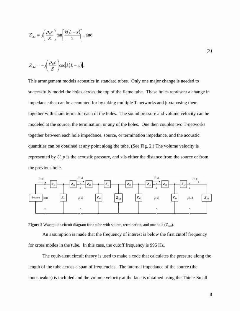
This arrangement models acoustics in standard tubes. Only one major change is needed to

successfully model the holes across the top of the flame tube. These holes represent a change in

impedance that can be accounted for by taking multiple T-networks and juxtaposing them

together with shunt terms for each of the holes. The sound pressure and volume velocity can be

modeled at the source, the termination, or any of the holes. One then couples two T-networks

together between each hole impedance, source, or termination impedance, and the acoustic

quantities can be obtained at any point along the tube. (See Fig. 2.) The volume velocity is

represented by U, p is the acoustic pressure, and x is either the distance from the source or from

the previous hole.

Figure 2 Waveguide circuit diagram for a tube with source, termination, and one hole (ZAH).

An assumption is made that the frequency of interest is below the first cutoff frequency

for cross modes in the tube. In this case, the cutoff frequency is 995 Hz.

The equivalent circuit theory is used to make a code that calculates the pressure along the

length of the tube across a span of frequencies. The internal impedance of the source (the

loudspeaker) is included and the volume velocity at the face is obtained using the Thiele-Small

8

parameters given later on in the report. The frequencies at which the pressure amplitude is a

local maximum are considered resonance frequencies. We use a computer to numerically

calculate the pressure at every point along the tube at all the frequencies of interest by

multiplying the impedance and the volume velocity together:

)()(ˆ)(ˆ xZxUxp ⋅= . (4)

B. Experiment

In order to analyze the accuracy of the hypothesis, we compare the numerical model to

experiment. The experiment required the construction of two new flame tubes to benchmark the

model.

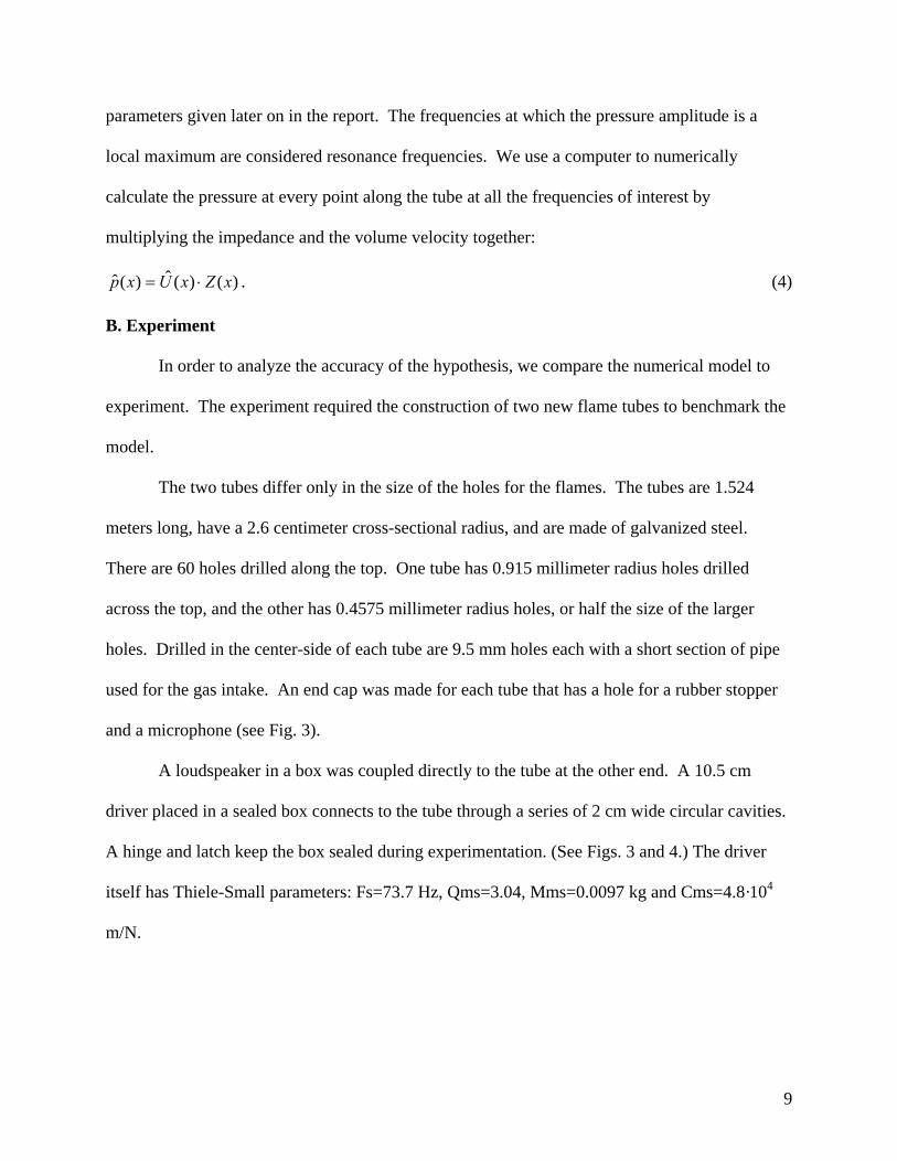
The two tubes differ only in the size of the holes for the flames. The tubes are 1.524

meters long, have a 2.6 centimeter cross-sectional radius, and are made of galvanized steel.

There are 60 holes drilled along the top. One tube has 0.915 millimeter radius holes drilled

across the top, and the other has 0.4575 millimeter radius holes, or half the size of the larger

holes. Drilled in the center-side of each tube are 9.5 mm holes each with a short section of pipe

used for the gas intake. An end cap was made for each tube that has a hole for a rubber stopper

and a microphone (see Fig. 3).

A loudspeaker in a box was coupled directly to the tube at the other end. A 10.5 cm

driver placed in a sealed box connects to the tube through a series of 2 cm wide circular cavities.

A hinge and latch keep the box sealed during experimentation. (See Figs. 3 and 4.) The driver

itself has Thiele-Small parameters: Fs=73.7 Hz, Qms=3.04, Mms=0.0097 kg and Cms=4.8·104

m/N.

9

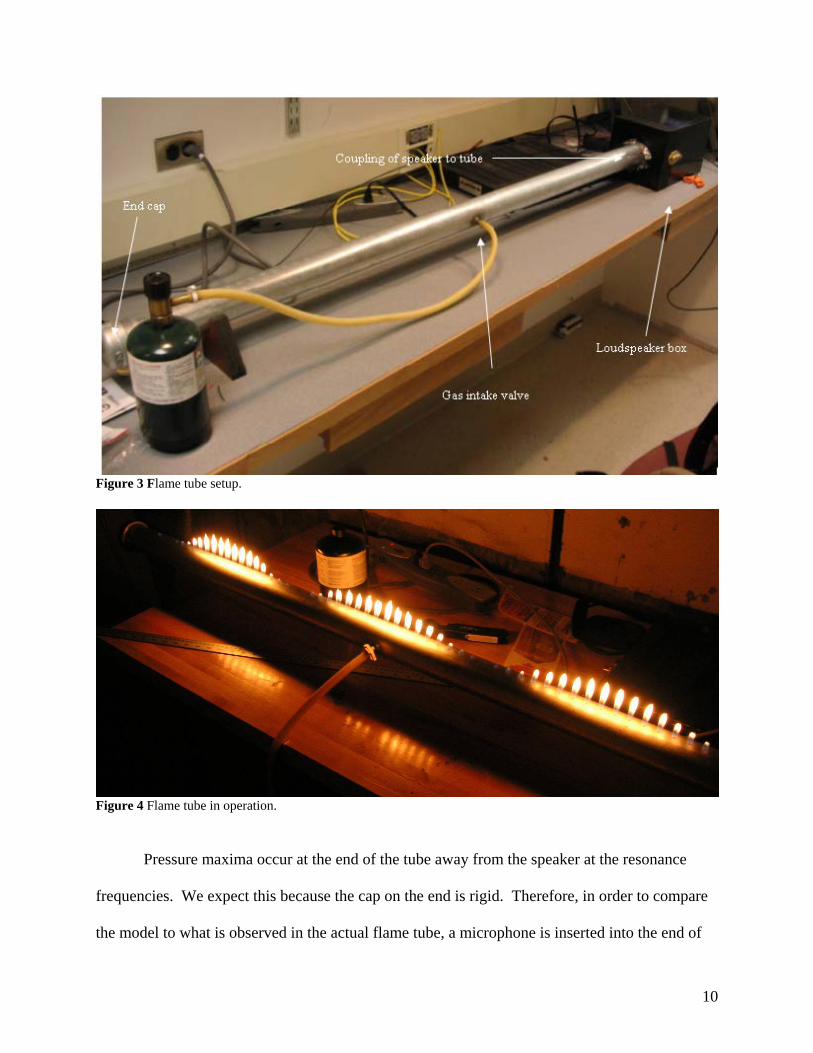
Figure 3 Flame tube setup.

Figure 4 Flame tube in operation.

Pressure maxima occur at the end of the tube away from the speaker at the resonance

frequencies. We expect this because the cap on the end is rigid. Therefore, in order to compare

the model to what is observed in the actual flame tube, a microphone is inserted into the end of

10

the tube. Random noise drives the loudspeaker, and the microphone records the frequency

response measurement of the pressure in the tube. In addition to measuring both tubes, this

experiment includes frequency response measurements of the tubes using both propane and air

inside the tube. The propane and air measurements give similar, supportive results. These

measured frequency responses become the benchmark or observed data to test the numerical

model.

Observations were also made pertaining to sound speed measurements. Knowing that

flame peaks occur at every node in the pressure during normal operation, the distance between

two peaks is one-half a wavelength. Observed data were taken by generating a flame pattern in

the tube at a certain frequency and measuring the distance between flame peaks and multiplying

the resultant wavelength by the frequency. This was done for several different modes.

III. RESULTS

This section will discuss the results of the numerical model and the comparison between the

model and the observed data.

A. Numerical model

A graphic user interface helps one to easily visualize the results of the numerical model.

The model is quite flexible. A user inputs into the model the relevant tube dimensions (tube

radius, hole spacing, number and size), the speed of sound, and density of the gas. The model

then outputs a graph of the magnitude of the pressure along the tube at whatever frequencies are

chosen. This can be seen in Figs. 5 and 6. Note that the actual magnitude in decibels is

irrelevant in all the remaining figures. The frequency is the more important quantity and the

magnitude is only used relatively as a marker for where the resonance frequencies occur.

11

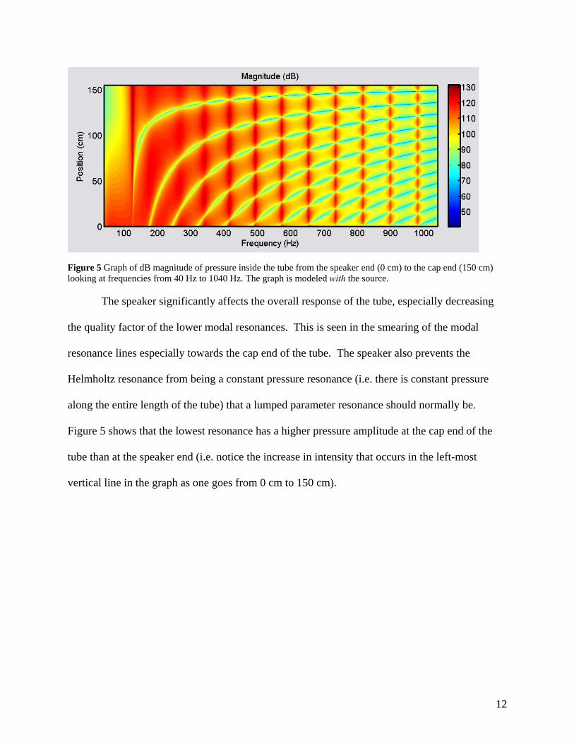
Figure 5 Graph of dB magnitude of pressure inside the tube from the speaker end (0 cm) to the cap end (150 cm) looking at frequencies from 40 Hz to 1040 Hz. The graph is modeled with the source.

The speaker significantly affects the overall response of the tube, especially decreasing

the quality factor of the lower modal resonances. This is seen in the smearing of the modal

resonance lines especially towards the cap end of the tube. The speaker also prevents the

Helmholtz resonance from being a constant pressure resonance (i.e. there is constant pressure

along the entire length of the tube) that a lumped parameter resonance should normally be.

Figure 5 shows that the lowest resonance has a higher pressure amplitude at the cap end of the

tube than at the speaker end (i.e. notice the increase in intensity that occurs in the left-most

vertical line in the graph as one goes from 0 cm to 150 cm).

12

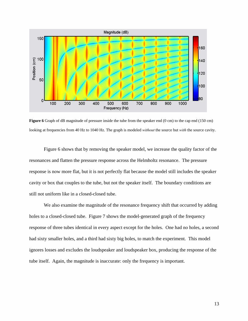
Figure 6 Graph of dB magnitude of pressure inside the tube from the speaker end (0 cm) to the cap end (150 cm)

looking at frequencies from 40 Hz to 1040 Hz. The graph is modeled without the source but with the source cavity.

Figure 6 shows that by removing the speaker model, we increase the quality factor of the

resonances and flatten the pressure response across the Helmholtz resonance. The pressure

response is now more flat, but it is not perfectly flat because the model still includes the speaker

cavity or box that couples to the tube, but not the speaker itself. The boundary conditions are

still not uniform like in a closed-closed tube.

We also examine the magnitude of the resonance frequency shift that occurred by adding

holes to a closed-closed tube. Figure 7 shows the model-generated graph of the frequency

response of three tubes identical in every aspect except for the holes. One had no holes, a second

had sixty smaller holes, and a third had sixty big holes, to match the experiment. This model

ignores losses and excludes the loudspeaker and loudspeaker box, producing the response of the

tube itself. Again, the magnitude is inaccurate: only the frequency is important.

13

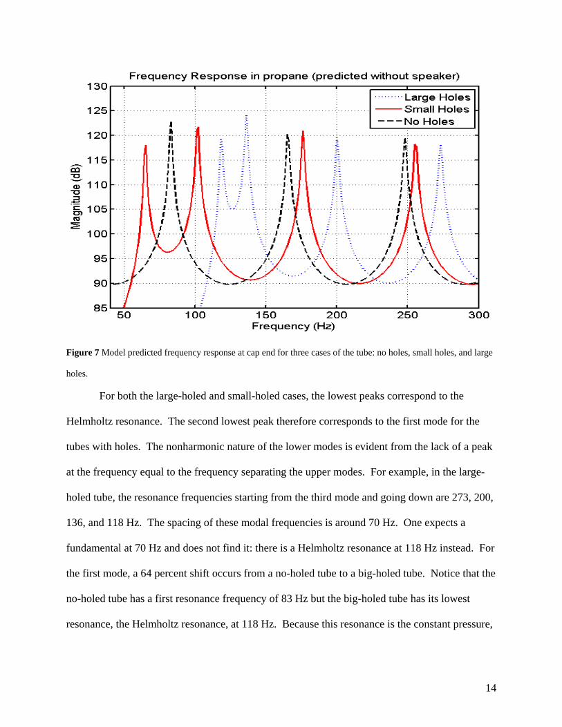
Figure 7 Model predicted frequency response at cap end for three cases of the tube: no holes, small holes, and large

holes.

For both the large-holed and small-holed cases, the lowest peaks correspond to the

Helmholtz resonance. The second lowest peak therefore corresponds to the first mode for the

tubes with holes. The nonharmonic nature of the lower modes is evident from the lack of a peak

at the frequency equal to the frequency separating the upper modes. For example, in the large-

holed tube, the resonance frequencies starting from the third mode and going down are 273, 200,

136, and 118 Hz. The spacing of these modal frequencies is around 70 Hz. One expects a

fundamental at 70 Hz and does not find it: there is a Helmholtz resonance at 118 Hz instead. For

the first mode, a 64 percent shift occurs from a no-holed tube to a big-holed tube. Notice that the

no-holed tube has a first resonance frequency of 83 Hz but the big-holed tube has its lowest

resonance, the Helmholtz resonance, at 118 Hz. Because this resonance is the constant pressure,

14

lumped parameter resonance, there can be no other resonances below it; therefore modal

resonances must shift to allow for this Helmholtz resonance.

B. Comparison of predicted and observed

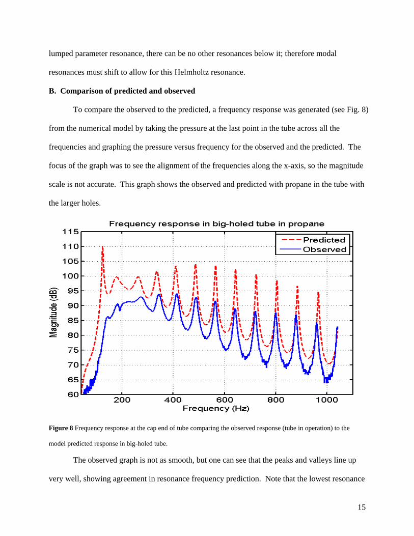
To compare the observed to the predicted, a frequency response was generated (see Fig. 8)

from the numerical model by taking the pressure at the last point in the tube across all the

frequencies and graphing the pressure versus frequency for the observed and the predicted. The

focus of the graph was to see the alignment of the frequencies along the x-axis, so the magnitude

scale is not accurate. This graph shows the observed and predicted with propane in the tube with

the larger holes.

Figure 8 Frequency response at the cap end of tube comparing the observed response (tube in operation) to the

model predicted response in big-holed tube.

The observed graph is not as smooth, but one can see that the peaks and valleys line up

very well, showing agreement in resonance frequency prediction. Note that the lowest resonance

15

peak for the observed response is quite small and does not match the quality factor of the

corresponding peak in the numerical model. This is not understood; however, the peak does

occur at the right frequency.

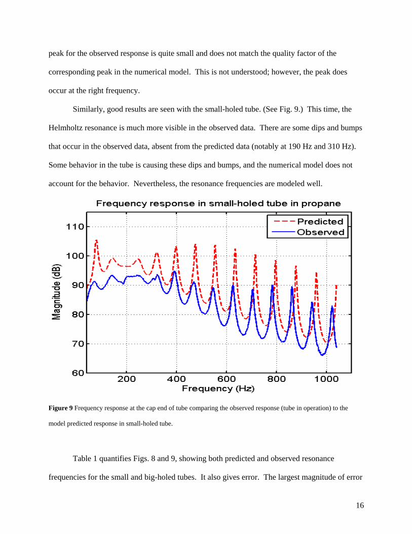
Similarly, good results are seen with the small-holed tube. (See Fig. 9.) This time, the

Helmholtz resonance is much more visible in the observed data. There are some dips and bumps

that occur in the observed data, absent from the predicted data (notably at 190 Hz and 310 Hz).

Some behavior in the tube is causing these dips and bumps, and the numerical model does not

account for the behavior. Nevertheless, the resonance frequencies are modeled well.

Figure 9 Frequency response at the cap end of tube comparing the observed response (tube in operation) to the

model predicted response in small-holed tube.

Table 1 quantifies Figs. 8 and 9, showing both predicted and observed resonance

frequencies for the small and big-holed tubes. It also gives error. The largest magnitude of error

16

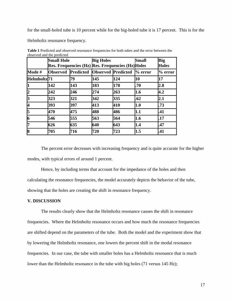
for the small-holed tube is 10 percent while for the big-holed tube it is 17 percent. This is for the

Helmholtz resonance frequency.

Table 1 Predicted and observed resonance frequencies for both tubes and the error between the observed and the predicted Small Hole

Res. Frequencies (Hz) Big Holes Res. Frequencies (Hz)

Small Holes

Big Holes

Mode # Observed Predicted Observed Predicted % error % error Helmholtz 71 79 145 124 10 17 1 142 143 183 178 .70 2.8 2 242 246 274 263 1.6 4.2 3 323 321 342 335 .62 2.1 4 393 397 413 410 1.0 .73 5 470 475 488 486 1.1 .41 6 546 555 563 564 1.6 .17 7 626 635 640 643 1.4 .47 8 705 716 720 723 1.5 .41

The percent error decreases with increasing frequency and is quite accurate for the higher

modes, with typical errors of around 1 percent.

Hence, by including terms that account for the impedance of the holes and then

calculating the resonance frequencies, the model accurately depicts the behavior of the tube,

showing that the holes are creating the shift in resonance frequency.

V. DISCUSSION

The results clearly show that the Helmholtz resonance causes the shift in resonance

frequencies. Where the Helmholtz resonance occurs and how much the resonance frequencies

are shifted depend on the parameters of the tube. Both the model and the experiment show that

by lowering the Helmholtz resonance, one lowers the percent shift in the modal resonance

frequencies. In our case, the tube with smaller holes has a Helmholtz resonance that is much

lower than the Helmholtz resonance in the tube with big holes (71 versus 145 Hz);

17

correspondingly, the resonance frequencies of the smaller-holed tube are not shifted as much.

This is useful information for those interested in building their own tube. The tube designer

controls how much the resonance frequencies are shifted.

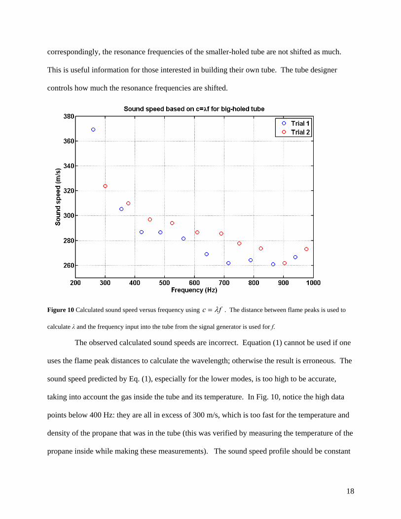
Figure 10 Calculated sound speed versus frequency using fc λ= . The distance between flame peaks is used to

calculate λ and the frequency input into the tube from the signal generator is used for f.

The observed calculated sound speeds are incorrect. Equation (1) cannot be used if one

uses the flame peak distances to calculate the wavelength; otherwise the result is erroneous. The

sound speed predicted by Eq. (1), especially for the lower modes, is too high to be accurate,

taking into account the gas inside the tube and its temperature. In Fig. 10, notice the high data

points below 400 Hz: they are all in excess of 300 m/s, which is too fast for the temperature and

density of the propane that was in the tube (this was verified by measuring the temperature of the

propane inside while making these measurements). The sound speed profile should be constant

18

across frequency because the speed of sound in a gas is dependent upon the medium and is

independent of frequency. The sound speeds for the higher frequencies are closer to the actual

sound speed. Therefore, the flame peak distance is not a reliable source for the wavelength in Eq.

(1).

In addition, the numerical model was used to generate a calculated sound speed profile

for the different resonance frequencies. As the frequency increases from the lowest resonance to

the highest, the sound speeds generated from the numerical model exhibit an exponential decay-

like trend that matches what is seen in the observed sound speeds (again, see Fig. 10): very high

sound speeds in the low frequencies converging to the actual sound speed at high frequencies.

The numerical model gives further evidence that the holes create this behavior. Consistent with

the resonance frequencies, the sound speeds calculated for the higher modes converge to the

actual sound speed in the tube based on the properties of the gas (propane, in this study). The

holes do not significantly affect the higher modes.

VI. CONCLUSIONS

The Rubens flame tube serves well as a classroom demonstration, but calculating

resonance frequencies or sound speeds is not a straightforward exercise of basic acoustics.

Depending on how the tube is built, the phenomena may or may not be strongly present. For

example, smaller and fewer holes will decrease the resonance frequency shift and will make the

sound speed measurements more accurate. The tube can be used as a demonstration of standing

waves in a closed-closed pipe or of parallel impedances and Helmholtz resonators, depending

upon the circumstance. Also, a teacher could demonstrate mainly the higher modes, which are

not affected as much, if he or she wanted to avoid the complicated behavior. Flame and gas flow

properties could be another demonstration. The flame tube has been around for over 100 years

19

but has been mostly unresearched. Professors and teachers should be aware of the complicated

nature of the flame tube when demonstrating it and at least be able to refer to explanatory articles

in order to better explain its behavior.

ACKNOWLEDGEMENTS

The author thanks Brigham Young University for the support in this research, including the

Office of Research and Creative Activities. The author also thanks Dr. Gee and Gordon Dix for

contributing significantly to the project.

1H. Rubens and O. Krigar-Menzel, "Flammenröhre für akustishe Beobachtungen (Flame tube for

acoustical observations)," Ann. Phys., Lpz. 17, 149 (1905).

2D. Jihui and C.T.P. Wang, “Demonstration of longitudinal standing waves in a pipe revisited,”

Am. J. Phys. 53, 11 (1985).

3G. Spagna, Jr., “Rubens flame tube demonstration: A closer look at the flames,” Am. J. Phys. 51,

9 (1983).

4H. Daw, “A two-dimensional flame table,” Am. J. Phys. 55, 8 (1987).

5G. Ficken and C. Stephenson “Rubens flame-tube demonstration” Phys. Teach. 17, 306 (1979).

20