an investigation of stokes' second problem for non-newtonian fluids

AN INVESTIGATION OF STOKES’ SECOND PROBLEMFOR NON-NEWTONIAN FLUIDS

L. Ai and K. VafaiDepartment of Mechanical Engineering, University of California at Riverside,Riverside, California, USA

Stokes flow produced by an oscillatory motion of a wall is analyzed in the presence of a non-

Newtonian fluid. A total of eight non-Newtonian models are considered. A mass balance

approach is introduced to solve the governing equations. The velocity and temperature pro-

files for these models are obtained and compared to those of Newtonian fluids. For the

power law model, correlations for the velocity distribution and the time required to reach

the steady periodic flow are developed and discussed. Furthermore, the effects of the dimen-

sionless parameters on the flow are studied. For the temperature distribution, an analytical

solution for Newtonian fluid is developed as a comparative source. To simulate the rheolo-

gical behavior of blood at unsteady state, three non-Newtonian constitutive relationships are

used to study the wall shear stress. It is found that in the case of unsteady stokes flow,

although the patterns of velocity and wall shear stress is consistent across all models, the

magnitude is affected by the model utilized.

1. INTRODUCTION

Stokes’ first problem refers to the shear flow of a viscous fluid near a flat platewhich is suddenly accelerated from rest and moves in its own plane with a constantvelocity. If the flat plate executes linear harmonic oscillations parallel to itself, theproblem is referred to as Stokes’ second problem [1]. It admits an analytical solution.The study of Stokes’ second problem has some applications in the fields of chemical,medical, biomedical, micro, and nanotechnology. An illustrative example is theshear-driven pump in microfluidic devices. The solution of the Stokes’ problemunder vibrating wall condition that satisfies the no-slip condition at the wall has beenstudied in depth by Erdogan [2]. Recently, exact solutions including both steady per-iodic and transient velocity profiles for Stokes’ and Couette flows subject to slip con-ditions were given in the work of Khaled and Vafai [3]. In the work of Johnston et al.[4], five non-Newtonian models for blood flow at steady state were studied.However, the literature lacks studies that take into account the presence ofnon-Newtonian fluids for Stokes’ second problem.

Among the non-Newtonian models, the second-grade model is able to predictthe normal stress differences which are characteristic of non-Newtonian fluids.However, the shear viscosity is constant in the second-grade model. As such, a

Received 15 September 2004; accepted 24 November 2004.

Address correspondence to K. Vafai, Department of Mechanical Engineering, A363 Bourns Hall,

University of California at Riverside, Riverside, CA 92521-0425, USA. E-mail: [email protected]

955

Numerical Heat Transfer, Part A, 47: 955–980, 2005

Copyright # Taylor & Francis Inc.

ISSN: 1040-7782 print=1521-0634 online

DOI: 10.1080/10407780590926390

shear-thinning or shear-thickening fluid cannot be predicted by a second-grademodel. The third-grade model exhibits shear-dependent viscosity. Examples can befound in chemical engineering, where in some industrial processes, steady andunsteady shear flows with non-Newtonian behavior are involved. In this work, thenon-Newtonian behavior for the Stokes second problem is investigated. As theshear-dependent viscosity models are introduced, the governing equations becomenonlinear. The solutions are obtained by using a mass balance argument to obtain adiscrete version of the governing equation. The mass balance approach [5] yieldsa system of difference equations that ensures the conservation of mass.

2. BASIC EQUATIONS

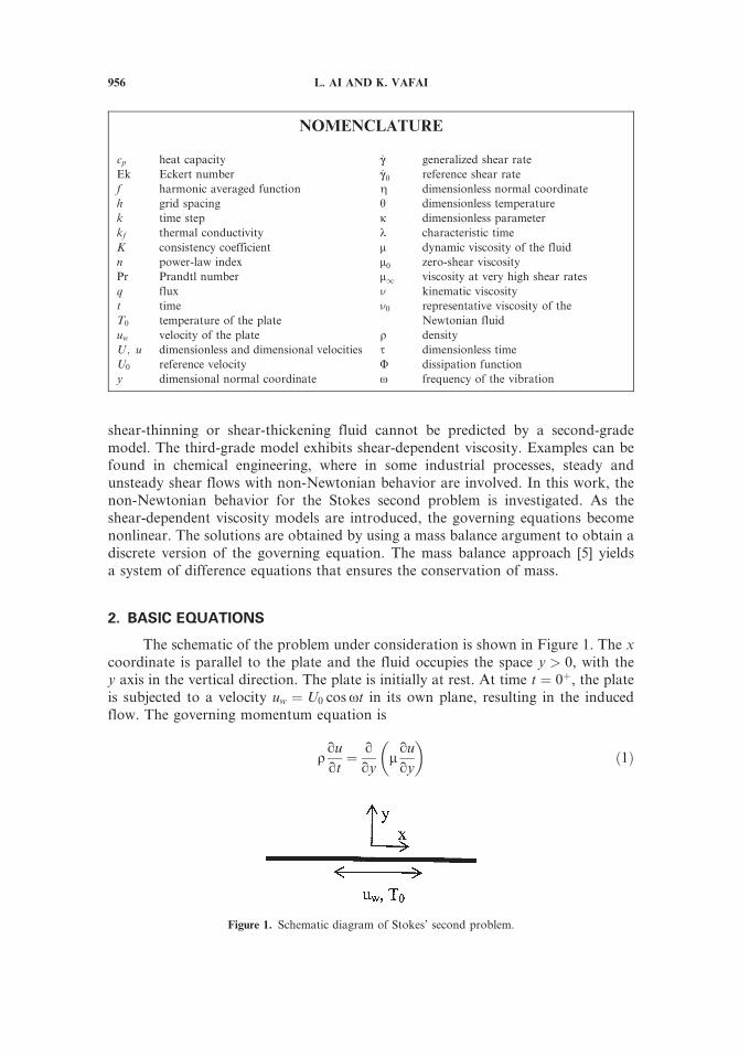
The schematic of the problem under consideration is shown in Figure 1. The xcoordinate is parallel to the plate and the fluid occupies the space y > 0, with they axis in the vertical direction. The plate is initially at rest. At time t ¼ 0þ, the plateis subjected to a velocity uw ¼ U0 cosxt in its own plane, resulting in the inducedflow. The governing momentum equation is

qquqt

¼ qqy

mquqy

� �ð1Þ

Figure 1. Schematic diagram of Stokes’ second problem.

NOMENCLATURE

cp heat capacity

Ek Eckert number

f harmonic averaged function

h grid spacing

k time step

kf thermal conductivity

K consistency coefficient

n power-law index

Pr Prandtl number

q flux

t time

T0 temperature of the plate

uw velocity of the plate

U ; u dimensionless and dimensional velocities

U0 reference velocity

y dimensional normal coordinate

_cc generalized shear rate_cc0 reference shear rate

g dimensionless normal coordinate

h dimensionless temperature

j dimensionless parameter

k characteristic time

m dynamic viscosity of the fluid

m0 zero-shear viscosity

m1 viscosity at very high shear rates

n kinematic viscosity

n0 representative viscosity of the

Newtonian fluid

q density

s dimensionless time

U dissipation function

x frequency of the vibration

956 L. AI AND K. VAFAI

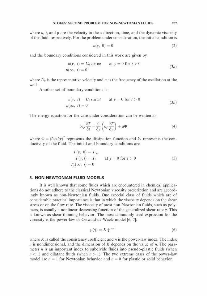
where u, t, and m are the velocity in the x direction, time, and the dynamic viscosityof the fluid, respectively. For the problem under consideration, the initial condition is

uðy; 0Þ ¼ 0 ð2Þ

and the boundary conditions considered in this work are given by

uðy; tÞ ¼ U0 cosxt at y ¼ 0 for t > 0

uð1; tÞ ¼ 0ð3aÞ

where U0 is the representative velocity and x is the frequency of the oscillation at thewall.

Another set of boundary conditions is

uðy; tÞ ¼ U0 sinxt at y ¼ 0 for t > 0

uð1; tÞ ¼ 0ð3bÞ

The energy equation for the case under consideration can be written as

qcpqTqt

¼ qqy

kfqTqy

� �þ mU ð4Þ

where U ¼ qu=qyð Þ2 represents the dissipation function and kf represents the con-ductivity of the fluid. The initial and boundary conditions are

Tðy; 0Þ ¼ T1

Tðy; tÞ ¼ T0 at y ¼ 0 for t > 0 ð5ÞTyð1; tÞ ¼ 0

3. NON-NEWTONIAN FLUID MODELS

It is well known that some fluids which are encountered in chemical applica-tions do not adhere to the classical Newtonian viscosity prescription and are accord-ingly known as non-Newtonian fluids. One especial class of fluids which are ofconsiderable practical importance is that in which the viscosity depends on the shearstress or on the flow rate. The viscosity of most non-Newtonian fluids, such as poly-mers, is usually a nonlinear decreasing function of the generalized shear rate _cc. Thisis known as shear-thinning behavior. The most commonly used expression for theviscosity is the power-law or Ostwald-de-Waele model [6, 7]:

mð _ccÞ ¼ K _ccj jn�1 ð6Þ

where K is called the consistency coefficient and n is the power-law index. The indexn is nondimensional, and the dimension of K depends on the value of n. The para-meter n is an important index to subdivide fluids into pseudo-plastic fluids (whenn < 1) and dilatant fluids (when n > 1). The two extreme cases of the power-lawmodel are n ¼ 1 for Newtonian behavior and n ¼ 0 for plastic or solid behavior.

STOKES’ SECOND PROBLEM FOR NON-NEWTONIAN FLUIDS 957

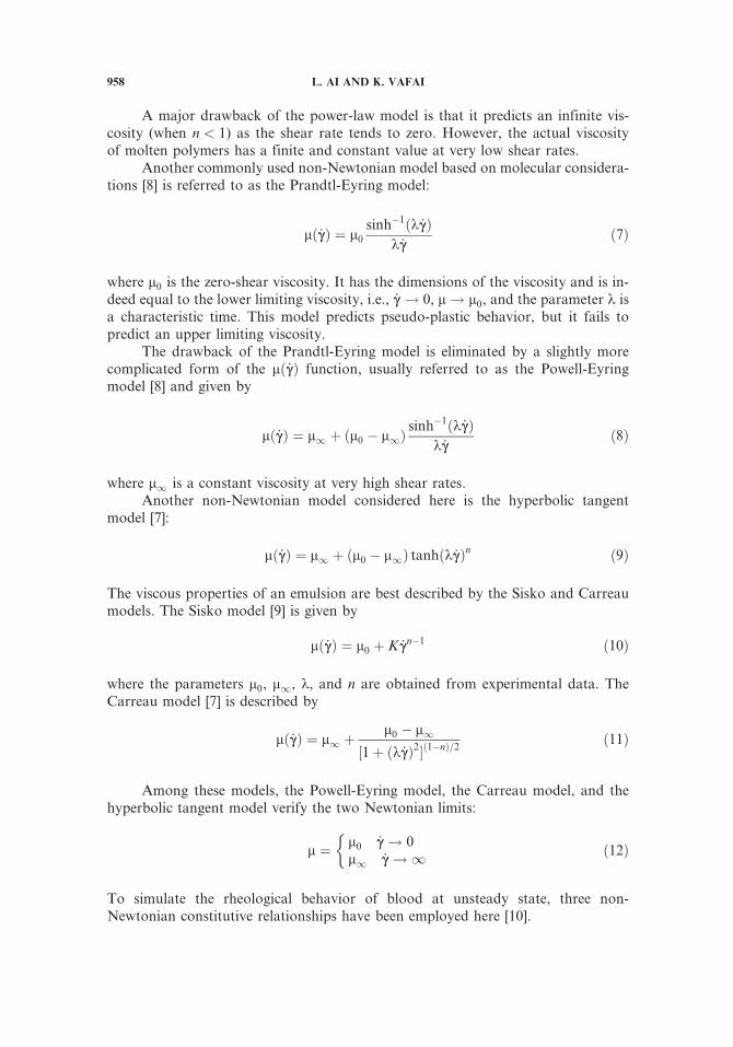
A major drawback of the power-law model is that it predicts an infinite vis-cosity (when n < 1) as the shear rate tends to zero. However, the actual viscosityof molten polymers has a finite and constant value at very low shear rates.

Another commonly used non-Newtonian model based on molecular considera-tions [8] is referred to as the Prandtl-Eyring model:

mð _ccÞ ¼ m0sinh�1ðk _ccÞ

k _ccð7Þ

where m0 is the zero-shear viscosity. It has the dimensions of the viscosity and is in-deed equal to the lower limiting viscosity, i.e., _cc ! 0, m ! m0, and the parameter k isa characteristic time. This model predicts pseudo-plastic behavior, but it fails topredict an upper limiting viscosity.

The drawback of the Prandtl-Eyring model is eliminated by a slightly morecomplicated form of the mð _ccÞ function, usually referred to as the Powell-Eyringmodel [8] and given by

mð _ccÞ ¼ m1 þ ðm0 � m1Þ sinh�1ðk _ccÞk _cc

ð8Þ

where m1 is a constant viscosity at very high shear rates.Another non-Newtonian model considered here is the hyperbolic tangent

model [7]:

mð _ccÞ ¼ m1 þ ðm0 � m1Þ tanhðk _ccÞn ð9Þ

The viscous properties of an emulsion are best described by the Sisko and Carreaumodels. The Sisko model [9] is given by

mð _ccÞ ¼ m0 þ K _ccn�1 ð10Þ

where the parameters m0, m1, k, and n are obtained from experimental data. TheCarreau model [7] is described by

mð _ccÞ ¼ m1 þ m0 � m1½1þ ðk _ccÞ2�ð1�nÞ=2 ð11Þ

Among these models, the Powell-Eyring model, the Carreau model, and thehyperbolic tangent model verify the two Newtonian limits:

m ¼ m0 _cc ! 0m1 _cc ! 1

�ð12Þ

To simulate the rheological behavior of blood at unsteady state, three non-Newtonian constitutive relationships have been employed here [10].


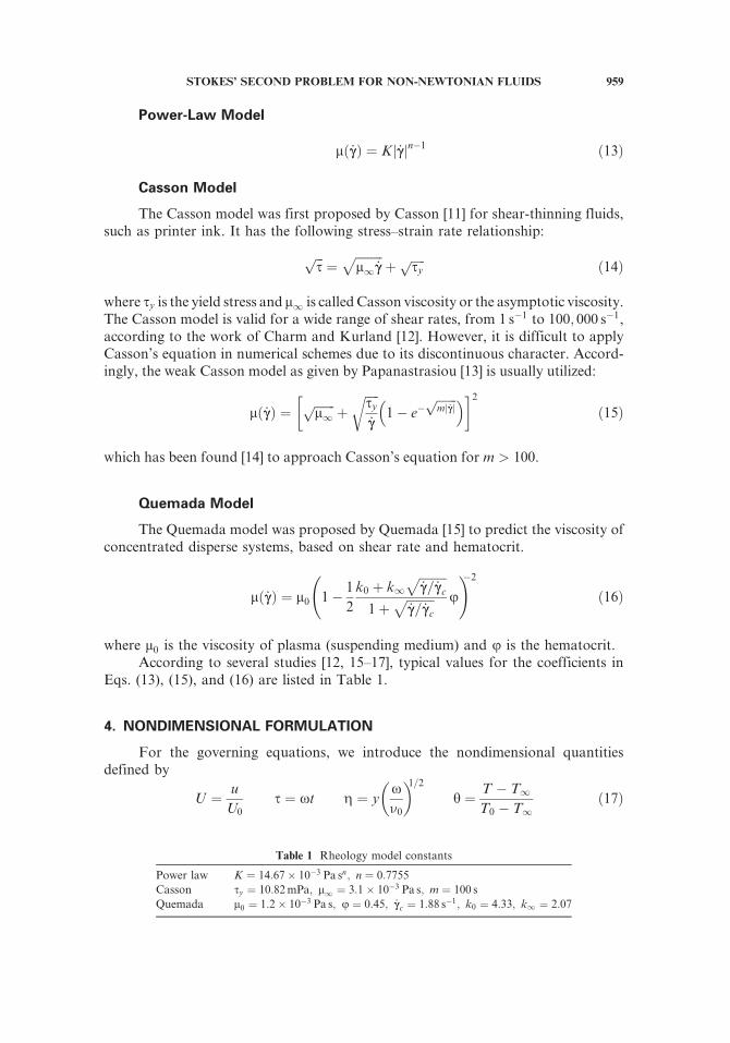
Power-Law Model

mð _ccÞ ¼ K _ccj jn�1 ð13Þ

Casson Model

The Casson model was first proposed by Casson [11] for shear-thinning fluids,such as printer ink. It has the following stress–strain rate relationship:

ffiffiffis

p¼

ffiffiffiffiffiffiffiffiffim1 _cc

pþ ffiffiffiffiffi

syp ð14Þ

where sy is the yield stress and m1 is called Casson viscosity or the asymptotic viscosity.The Casson model is valid for a wide range of shear rates, from 1 s�1 to 100; 000 s�1,according to the work of Charm and Kurland [12]. However, it is difficult to applyCasson’s equation in numerical schemes due to its discontinuous character. Accord-ingly, the weak Casson model as given by Papanastrasiou [13] is usually utilized:

mð _ccÞ ¼ ffiffiffiffiffiffiffim1

p þffiffiffiffiffisy_cc

r1� e�

ffiffiffiffiffiffiffim _ccj j

p� �� 2ð15Þ

which has been found [14] to approach Casson’s equation for m > 100.

Quemada Model

The Quemada model was proposed by Quemada [15] to predict the viscosity ofconcentrated disperse systems, based on shear rate and hematocrit.

mð _ccÞ ¼ m0 1� 1

2

k0 þ k1ffiffiffiffiffiffiffiffiffi_cc= _ccc

p1þ

ffiffiffiffiffiffiffiffiffi_cc= _ccc

p u

!�2

ð16Þ

where m0 is the viscosity of plasma (suspending medium) and u is the hematocrit.According to several studies [12, 15–17], typical values for the coefficients in

Eqs. (13), (15), and (16) are listed in Table 1.

4. NONDIMENSIONAL FORMULATION

For the governing equations, we introduce the nondimensional quantitiesdefined by

U ¼ u

U0s ¼ xt g ¼ y

xn0

� �1=2h ¼ T � T1

T0 � T1ð17Þ

Table 1 Rheology model constants

Power law K ¼ 14:67� 10�3 Pa sn; n ¼ 0:7755

Casson sy ¼ 10:82mPa; m1 ¼ 3:1� 10�3 Pa s; m ¼ 100 s

Quemada m0 ¼ 1:2� 10�3 Pa s; u ¼ 0:45; _ccc ¼ 1:88 s�1; k0 ¼ 4:33; k1 ¼ 2:07


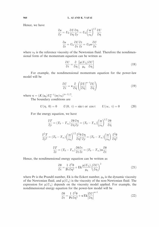
Hence, we have

quqy

¼ U0qUqg

qgqy

¼ U0xn0

� �1=2 qUqg

quqt

¼ U0qUqs

qsqt

¼ U0xqUqs

where n0 is the reference viscosity of the Newtonian fluid. Therefore the nondimen-sional form of the momentum equation can be written as

qUqs

¼ qqg

mðUgÞm0

qUqg

� �ð18Þ

For example, the nondimensional momentum equation for the power-lawmodel will be

qUqs

¼ jqqg

qUqg

n�1qU

qg

!ð19Þ

where j ¼ K=m0ð ÞUn�10 ðx=n0Þðn�1Þ=2.

The boundary conditions are

Uðg; 0Þ ¼ 0 Uð0; sÞ ¼ sin s or cos s Uð1; sÞ ¼ 0 ð20Þ

For the energy equation, we have

qTqy

¼ ðT0 � T1Þ qhqg

qgqy

¼ ðT0 � T1Þ xn0

� �1=2 qhqg

q2Tqy2


� �1=2 q2hqg2

qgqy


� �q2hqg2

qTqt

¼ ðT0 � T1Þ qhqs

qsqt

¼ ðT0 � T1Þx qhqs

Hence, the nondimensional energy equation can be written as

qhqs

¼ 1

Pr

q2hqg2

þ EkmðUgÞm0

qUqg

� �2

ð21Þ

where Pr is the Prandtl number, Ek is the Eckert number, m0 is the dynamic viscosityof the Newtonian fluid, and mðUgÞ is the viscosity of the non-Newtonian fluid. Theexpression for mðUgÞ depends on the viscosity model applied. For example, thenondimensional energy equation for the power-law model will be

qhqs

¼ 1

Pr

q2hqg2

þ jEkqUqg

nþ1

ð22Þ


where j ¼ K=m0ð ÞUn�10 ðx=n0Þðn�1Þ=2. And the temperature boundary and initial con-

ditions can be written as

hð0; sÞ ¼ 1 hgð1; sÞ ¼ 0 hðg; 0Þ ¼ 0 ð23Þ

5. NUMERICAL SIMULATION

An effective finite-difference procedure is developed to solve the nonlinearequations. A material balance argument is utilized to obtain the discrete versionof the nonlinear momentum equation. To illustrate a material balance approachin developing difference equations, we use the following notation to simplify thenondimensional version of the momentum equation:

sðuÞut � ½aðuÞux�x ¼ 0 ð24Þ

Equation (24) represents a conservation law in the sense that a density q and a flux qcan be related to u with equations of the form qt ¼ sðuÞut and q ¼ �aðuÞux, so thatthat Eq. (24) is equivalent to the balance equation

qt þ qx ¼ 0 ð25Þ

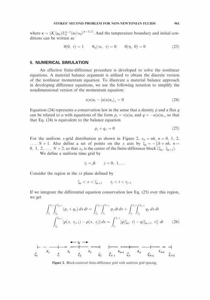
For the uniform x-grid distribution as shown in Figure 2, xn ¼ nh, n ¼ 0; 1; 2;. . . ; N þ 1. Also define a set of points on the x axis by nn ¼ � 1

2 hþ nh, n ¼0; 1; 2; . . . ; N þ 2, so that xn is the center of the finite-difference block ðnn; nnþ1Þ.

We define a uniform time grid by

tj ¼ jk j ¼ 0; 1; . . .

Consider the region in the xt plane defined by

nn < x < nnþ1 tj < t < tjþ1

If we integrate the differential equation conservation law Eq. (25) over this region,we get

Z tjþ1

tj

Z nnþ1

nn

ðqt þ qxÞ dx dt ¼Z nnþ1

nn

Z tjþ1

tj

qt dt dxþZ tjþ1

tj

Z nnþ1

nn

qx dx dt

Z nnþ1

nn

½qðx; tjþ1Þ � qðx; tjÞ� dx ¼Z tjþ1

tj

½qðnn; tÞ � qðnnþ1; tÞ� dt ð26Þ

Figure 2. Block-centered finite-difference grid with uniform grid spacing.


We will use the midpoint quadrature rule to approximate the integral of the densitiesin Eq. (26): Z nnþ1

nn

½qðx; tjþ1Þ � qðx; tjÞ� dx ffi ½qðxn; tjþ1Þ � qðxn; tjÞ�h ð27Þ

To approximate the integral of the fluxes in Eq. (26) in a manner consistentwith the implicit, backward-in-time method, we choose the right endpoint quadra-ture rule to obtainZ tjþ1

tj

½qðnn; tÞ � qðnnþ1; tÞ� dt ¼ ½qðnn; tjþ1Þ � qðnnþ1; tjþ1Þ�k ð28Þ

Here we use the trapezoidal rule to approximate Eq. (28):

½qðxn; tjþ1Þ � qðxn; tjÞ�h ¼ ½qðnn; tjþ1Þ � qðnnþ1; tjþ1Þ�k ð29Þ

From q ¼ �aðuÞux, we have

uxðx; tjþ1Þ ¼ � qðx; tjþ1Þa½uðx; tjþ1Þ�

ð30Þ

The integral of Eq. (30) from xn�1 to xn gives

u jþ1n � u jþ1

n�1 ¼ �Z xn

xn�1

qðx; tjþ1Þa½x; uðx; tjþ1�

dx ffi �qðnn; tjþ1Þhða jþ1

n þ a jþ1n�1 Þ

2a jþ1n a jþ1

n�1

( )ð31Þ

We introduce the harmonic averaged function as

f ðam; anÞ ¼2amanam þ an

ð32Þ

Also, to avoid a division by zero, we define f ð0; 0Þ ¼ 0.Hence we have

qðnn; tjþ1Þ ffi � 2a jþ1n a jþ1

n�1

ða jþ1n þ a jþ1

n�1Þu jþ1n � u jþ1

n�1

hor

qðnn; tjþ1Þ ffi �f ða jþ1n ; a jþ1

n�1Þ½ujþ1n � u jþ1

n�1 �=h ð33Þ

For the problem under consideration, we have

p ¼ U q ¼ � mðUgÞm0

qUqg

aðuÞ ¼ mðUgÞm0

ð34Þ

Introducing the notation

f jþ1n�1 ¼ f ða jþ1

n ; a jþ1n�1Þ f jþ1

nþ1 ¼ f ða jþ1n ; a jþ1

nþ1Þ ð35Þ


The nondimensionalized momentum equation can be expressed as

U jþ1n �Uj

n ¼ r f jþ1n�1 U

jþ1n�1 � f jþ1

n�1 þ f jþ1nþ1

� �U jþ1

n þ f jþ1nþ1 U

jþ1nþ1

h ið36Þ

where r ¼ k=h2.The usual first approximation to the solution of the nonlinear difference equa-

tion is obtained by ‘‘lagging the nonlinearities.’’ That is, the coefficients in the differ-ence equation are set at the t value, rather than the tþ k value. If the nonlinearitiesin Eq. (36) are lagged, the result is the linear system

U jþ1n �Uj

n ¼ r f jn�1Ujþ1n�1 � f jn�1 þ f jnþ1

� �U jþ1

n þ f jnþ1Ujþ1nþ1

h ið37Þ

Using a procedure similar to the Crank-Nicholson method, we get the finite-differenceequation as

� r

2f jn�1U

jþ1n�1 þ 1þ r

2f jn�1 þ f jnþ1

� �h iU jþ1

n

� r

2fjnþ1U

jþ1nþ1 ¼ Uj

nð1� rÞ þ r

2U

jn�1 þU

jnþ1

� �ð38Þ

Since we have already obtained the velocity gradient, namely, ðUgÞjn, in the process ofsolving themomentumequation,we introduce theCrank-Nicholsonmethod todiscretizethe energy equation given by Eq. (21).

Similarly, the finite-difference form of the energy equation can then beobtained as

h jþ1n � hjn ¼

1

Pr

k

2h2h jþ1n�1 � 2h jþ1

n þ h jþ1nþ1 þ h j

n�1 � 2h jn þ h j

nþ1

� �þ Ek

mjnm0

Ug �j

n

h i2ð39Þ

or

� 1

Pr

r

2h jþ1n�1 þ 1þ r

Pr

� �h jþ1n � 1

Pr

r

2h jþ1nþ1 ¼ 1� r

Pr

� �h jn

þ 1

Pr

r

2h jn�1 þ h j

nþ1

� �þ Ek

m jn

m0Ug � j

n

h i2ð40Þ

where r ¼ k=h2.For a Newtonian fluid, an analytical solution for the temperature distribution

is established utilizing the classical analytical velocity distribution and using thefollowing transformation:

s ¼ffiffiffiffiffiPr

pg ð41Þ

Equation (21) can then be written as

qhqs

¼ q2hqs2

þ PrEkqUqs

� �2ð42Þ


where qU=qs can be obtained from the velocity solution of Erdogan [2] or Khaledand Vafai [3] for the no-slip case.

The initial and boundary conditions will be

hð0; sÞ ¼ 1 hsð1; sÞ ¼ 0 hðs; 0Þ ¼ 0 ð43Þ

Letting gðs; sÞ ¼ Pr EkðqU=qsÞ2, the solution of Eq. (42) can be formed as [18]

hðg; sÞ ¼ s

2ffiffiffip

pZ s

t¼0

1

ðs� tÞ3=2e�½s2=4ðs�tÞ� dtþ 1

2ffiffiffip

pZ s

t¼0

1ffiffiffiffiffiffiffiffiffiffis� t

pZ 1

x¼0

gðx; tÞ

� fe�½ðs�xÞ2=4ðs�tÞ� � e�½ðsþxÞ2=4ðs�tÞ�g dx dt ð44Þ

6. NUMERICAL SIMULATION AND DISCUSSION

Numerical results for the nondimensional velocity Uðg; sÞ have been obtainedfor each boundary condition and for various viscosity models. It has been foundthat the non-Newtonian flows also achieve a steady periodic state. It should be notedthat when the power index n ¼ 1 for the power-law model or when the generalizedshear rate _cc ! 0 for other models, the numerical results obtained here agree wellwith the exact solution of Khaled and Vafai [3] for the Newtonian flow with no-slipcondition.

In Figure 3a, the velocity profile is presented when the boundary condition isuw ¼ U0 sinwt for various values of power index n for the power-law model. The valueat n ¼ 1 refers to a Newtonian fluid. The following correlation is obtained for calcu-lating the velocity distribution with the power-index range from n ¼ 0:6 to n ¼ 1:6:

U ¼ UN þ 2:4� ð�0:18g3 þ 0:55g2:5 þ g0:9Þ � expð�2:35g0:57n0:16Þ� cosðs� 2:35g0:57n0:16Þ � ½ðn� 1Þ�1:27ðn� 1Þ2 þ 0:88ðn� 1Þ3�� cosð�0:08g1:28n1:8 þ 1:5Þ ð45Þ

where UN is the classical analytical velocity distribution for a Newtonian fluid.Figure 4a illustrates the effects of the power index n on the time required to

reach steady periodic flow under the boundary condition utilized in Figure 3a. Thetime required to reach steady periodic flow was evaluated based on the dimensionlesstime for the average dimensionless transient velocity reaching a value of 0.05. Theresults show that power index strongly affects the time required for reaching steadyperiodic flow conditions. A power-index value of n ’ 0:65 is found to correspond tothe maximum time required to reach steady periodic flow conditions. Dimensionlessparameter j ¼ ðK=m0ÞUn�1

0 ðx=n0Þðn�1Þ=2 in Eq. (19) corresponds to 1 in this case. Forthe power-index range from n ¼ 0:2 to n ¼ 1:6, the following correlation is obtainedfor calculating time required for reaching steady periodic flow conditions:

s ¼ 0:2797þ 0:9229nþ 1:9433n2 � 3:5901n3

1� 3:311nþ 6:0743n2 � 4:1052n3 þ 0:1274n4ð46Þ


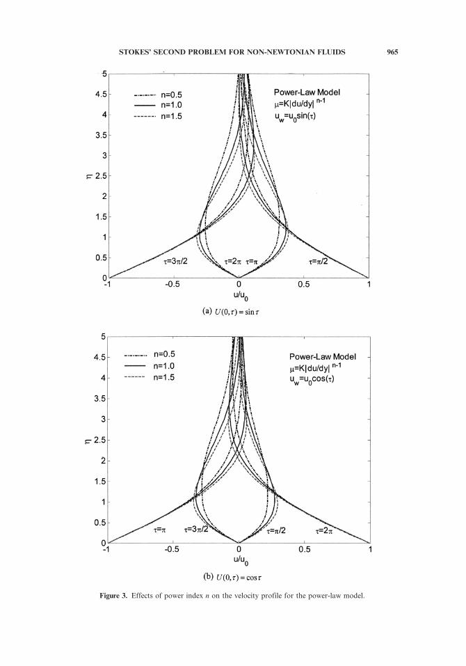
Figure 3. Effects of power index n on the velocity profile for the power-law model.


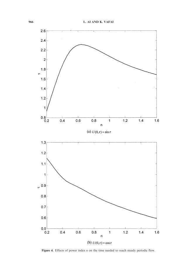
Figure 4. Effects of power index n on the time needed to reach steady periodic flow.


In Figure 3b, the velocity profile is presented when the boundary condition isuw ¼ U0 coswt for various values of the power index n in the power-law model. Fig-ure 4b illustrates the effects of the power index n on the time required to reach steadyperiodic flow under the cosine boundary condition. Comparing Figures 3a and 3b,we can see that the effect of the boundary condition is more pronounced than theeffect of the power index. For the power-index range from n ¼ 0:2 to n ¼ 1:6, thefollowing correlation is obtained for calculating the time required for reaching steadyperiodic flow conditions when the cosine boundary condition is specified at the wall:

s ¼ 1:5984� 8:1767nþ 11:9971n2 � 2:4893n3 � 1:8727n4

1� 2:8162n� 5:1123n2 þ 20:4959n3 � 12:9093n4 þ 1:0513n5ð47Þ

Our results illustrate that an increase in the power index delays the oscillatoryboundary condition effects shown in Figures 3a and 3b.

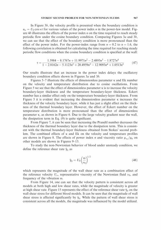
Figures 5–7 illustrate the effects of dimensionless parameter j and Ek numberon the velocity and temperature distribution due to cosine oscillations. FromFigure 5 we see that the effect of dimensionless parameter j is to increase the velocityboundary-layer thickness and the temperature boundary-layer thickness. Eckertnumber has a similar effect only on the temperature boundary-layer thickness. FromFigure 5 it is evident that increasing the dimensionless parameter j increases thethickness of the velocity boundary layer, while it has just a slight effect on the thick-ness of the thermal boundary layer. However, the effect of Eckert number on thetemperature distribution is more pronounced than the effect of dimensionlessparameter j, as shown in Figure 6. Due to the large velocity gradient near the wall,the dissipation term in Eq. (9) is quite significant.

From Figure 7, it can be seen that increasing the Prandtl number decreases thethickness of the thermal boundary layer due to the dissipation term. This is consist-ent with the thermal boundary-layer thickness obtained from Stokes’ second prob-lem. The combined effects of j and Ek on the velocity and temperature profilesare shown in Figure 8. The effects of power index n and viscosity ratio m1=m0 onother models are shown in Figures 9–13.

To study the non-Newtonian behavior of blood under unsteady condition, wedefine the reference shear rate _cc0 as

_cc0 ¼ U0xn0

� �1=2ð48Þ

which represents the magnitude of the wall shear rate as a combination effect ofthe reference velocity Uo, representative viscosity of the Newtonian fluid n0, andfrequency of the vibration x.

From Figure 14, one can see that the velocity pattern is consistent across allmodels at both high and low shear rates, while the magnitude of velocity is greaterat high shear rate. Figure 15 represents the effect of the reference shear rate _cc0 on thewall shear stress for different blood models. It can be seen that the magnitude of wallshear stress is affected significantly by _cc0. While the pattern of wall shear stress isconsistent across all the models, the magnitude was influenced by the model utilized.


Figure 5. Effects of parameter j on the velocity and temperature profiles for the power-law model.


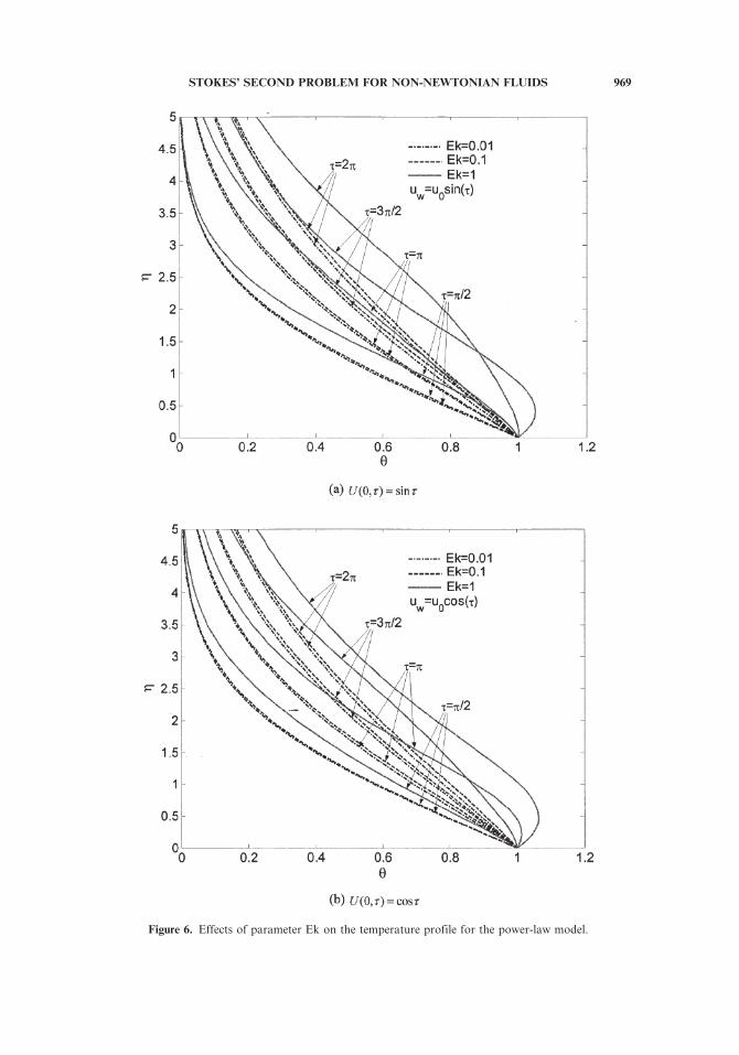
Figure 6. Effects of parameter Ek on the temperature profile for the power-law model.


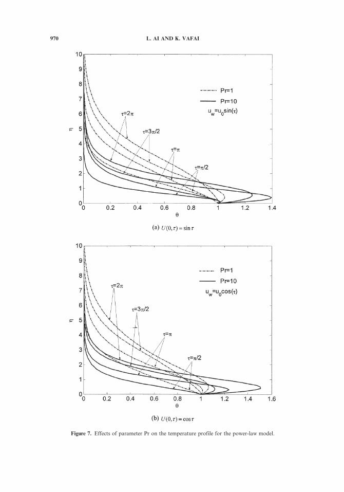
Figure 7. Effects of parameter Pr on the temperature profile for the power-law model.


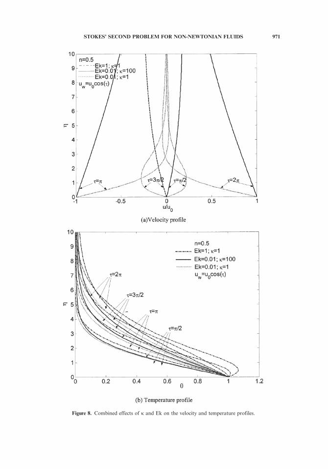
Figure 8. Combined effects of j and Ek on the velocity and temperature profiles.


Figure 9. Effects of viscosity ratio m1=m0 on the velocity profile for the Powell-Eyring model.


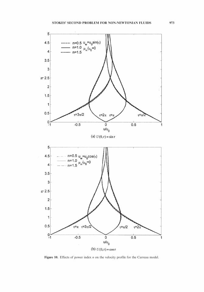
Figure 10. Effects of power index n on the velocity profile for the Carreau model.


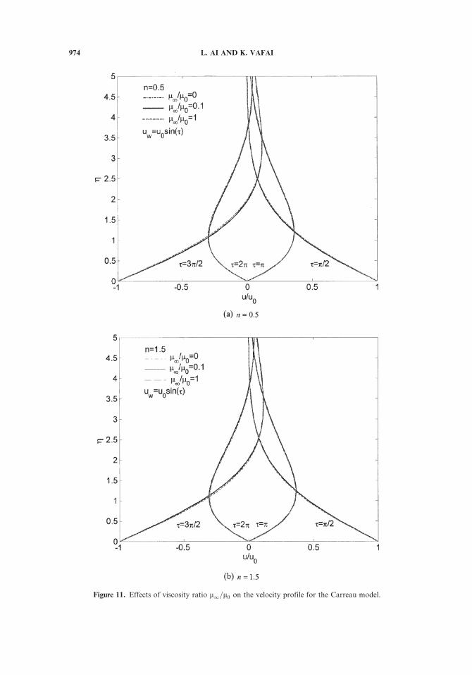
Figure 11. Effects of viscosity ratio m1=m0 on the velocity profile for the Carreau model.


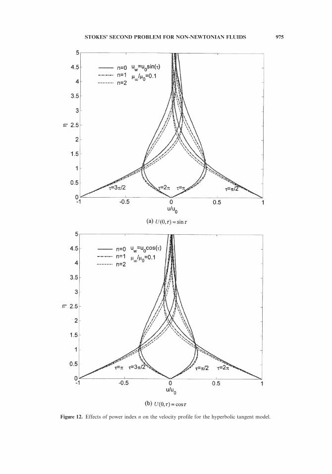
Figure 12. Effects of power index n on the velocity profile for the hyperbolic tangent model.


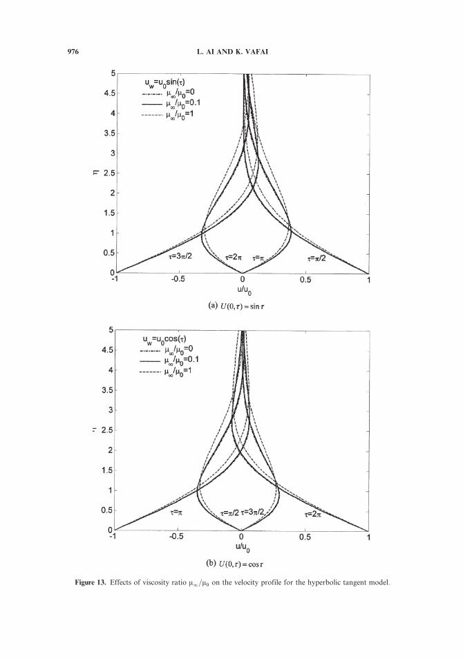
Figure 13. Effects of viscosity ratio m1=m0 on the velocity profile for the hyperbolic tangent model.


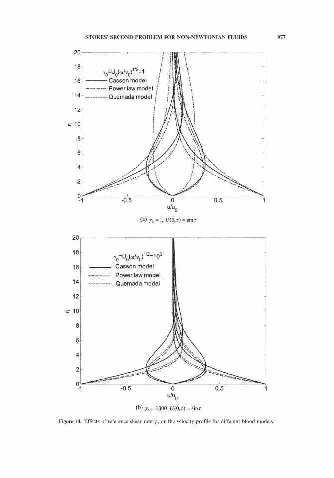
Figure 14. Effects of reference shear rate c0 on the velocity profile for different blood models.


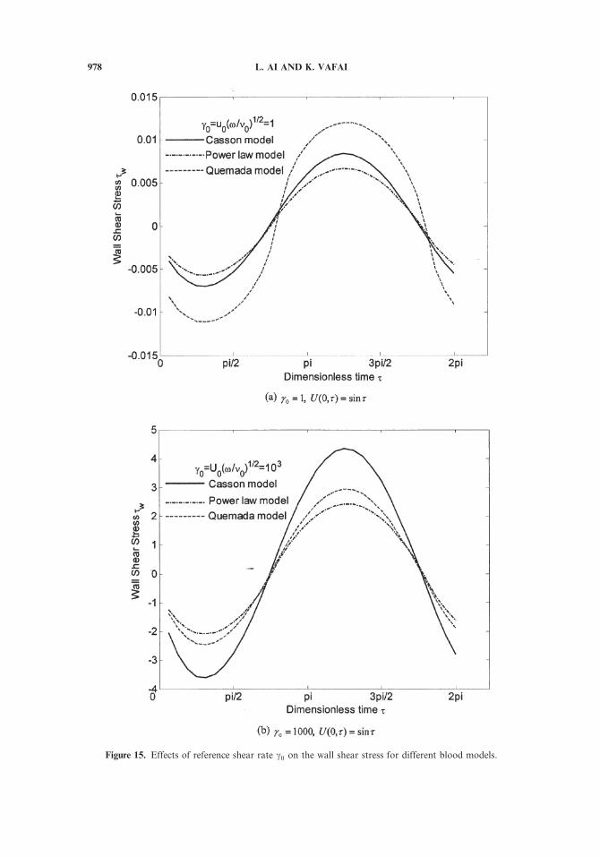
Figure 15. Effects of reference shear rate c0 on the wall shear stress for different blood models.


7. CONCLUSIONS

In this article, effects of non-Newtonian flow on Stokes’ second problem wereinvestigated. The wall was subjected to both sine and cosine oscillations. The tem-perature variation near the wall was also investigated. Several pertinent viscositymodels for non-Newtonian fluids were introduced. The governing equations werenondimensionalized and solved by introducing a mass-balance procedure. The velo-city and temperature profiles for various viscosity models were obtained and theresults were compared to those obtained for the Newtonian fluids. For the power-law model, the time required to reach steady periodic flow for various power-lawindices was established. Correlations for the velocity distribution and the time requiredto reach steady periodic flow conditions were developed. The effects of the dimen-sionless parameters, such as power index n and Ek, on the flow were analyzed, and ananalytical solution for the temperature distribution for the Newtonian case wasobtained. It was also found that in the case of unsteady Stokes flow, while the flowpatterns are consistent across all models, the magnitude was affected significantly bythe reference shear rate and the model utilized.

REFERENCES

1. H. Schilichting, Boundary Layer Theory, 6th ed., McGraw-Hill, New York, 1968.2. M. E. Erdogan, A Note on Unsteady Flow of a Viscous Fluid due to an Oscillating Plane

Wall, Int. J. Non-Linear Mech., vol. 35, pp. 1–6, 2000.3. A.-R. A. Khaled and K. Vafai, The Effect of the Slip Condition on Stokes and Couette

Flows due to an Oscillating Wall: Exact Solutions, Int. J. Non-Linear Mech., vol. 39,pp. 795–809, 2004.

4. B. M. Johnston, P. R. Johnston, S. Corney, and D. Kilpatrick, Non-Newtonian BloodFlow in Human Right Coronary Arteries: Steady State Simulations, J. Biomech.,vol. 37, pp. 709–720, 2004.

5. E. L. Allgower and K. Georg, Computational Solution of Nonlinear Systems of Equations,American Mathematical Society, Providence, RI, 1990.

6. J. F. Agassant, P. Avenas, J. Ph. Sergent, and P. J. Carreau, Polymer Processing: Princi-ples and Modeling, Hanser, New York, 1991.

7. I. Pop and D. B. Ingham, Convective Heat Transfer: Mathematical and ComputationalModelling of Viscous Fluids and Porous Media, Pergamon, Amsterdam, New York, 2001.

8. G. Astarita and G. Marrucci, Principles of Non-Newtonian Fluid Mechanics, McGraw-Hill, New York, 1974.

9. A. H. P. Skelland, Non-Newtonian Flow and Heat Transfer, Wiley, New York, 1967.10. P. Neofytou and D. Drikakis, Non-Newtonian Flow Instability in a Channel with a Sud-

den Expansion, J. Non-Newtonian Fluid Mech., vol. 111, pp. 127–150, 2003.11. N. Casson, A Flow Equation for the Pigment Oil Suspensions of the Printing Ink Type, in

Rheology of Disperse Systems, pp. 84–102, Pergamon, New York, 1959.12. S. Charm and G. Kurland, Viscometry of Human Blood for Shear Rates of 0–100,000 s�1.

Nuture (Lond.), vol. 206, pp. 617–618, 1965.13. T. C. Papanastasiou, Flows of Materials with Yield, J. Rheol., vol. 31, pp. 385–404, 1987.14. T. V. Pham and E. Mitsoulis, Entry and Exit Flows of Casson Fluids, Can. J. Chem. Eng.,

vol. 72, p. 1080, 1994.


15. D. Quemada, Rheology of Concentrated Disperse Systems. III. General Features of theProposed Non-Newtonian Model. Comparison with Experimental Data, Rheol. Acta,vol. 17, p. 643, 1977.

16. S. E. Charm, W. McComis, and G. Kurland, Rheology and Structure of Blood Suspen-sion, J. Appl. Physiol., vol. 19, p. 127, 1964.

17. F. J. Walburn and D. J. Schneck, A Constitutive Equation for Whole Human Blood,Biorheology, vol. 13, p. 201, 1976.

18. M. D. Mikhailov and M. N. Ozisik, Unified Analysis and Solutions of Heat and MassDiffusion, Wiley, New York, 1984.


Documents

an investigation of stokes' second problem for non-newtonian fluids