Embed Size (px)
Citation preview

An Investigation of the Relationship between Crime and Reported
Incidents and the Built and Natural Environment in the Region of
Waterloo, Ontario
by
Gregory James Metcalfe
A thesis
presented to the University Of Waterloo
in fulfilment of the
thesis requirement for the degree of
Master of Science
in
Geography
Waterloo, Ontario, Canada, 2017
© Gregory James Metcalfe 2017

ii
Author's declaration
I hereby declare that I am the sole author of this thesis. This is a true copy of the thesis,
including any required final revisions, as accepted by my examiners.
I understand that my thesis may be made electronically available to the public.

iii
Abstract
In the study of crime and geography, many studies have investigated the spatial
relationship between crime and the built and natural environment. However, these studies
usually focus on specific environmental characteristics, such as alcohol serving businesses or the
presence of vegetation. This study conducts a comprehensive analysis of the spatial relationship
between crime and features of the built and natural environment in the sister cities of Kitchener
and Waterloo, Ontario, taking into account many factors that may potentially affect crime and
reported incidents. This includes built environment features, such as residential buildings,
commercial buildings, drinking establishments, and bus stops. Natural environment features,
such as parks and the presence of green vegetation were also considered. The measure of crime
in this study was a geospatial record (aggregated to the nearest street intersection) of crime and
reported incidents where police were called (e.g., emergency call and response) recorded by the
Waterloo Regional Police Service (WRPS). Relationships between built and natural environment
characteristics with crime and reported incidents were studied using linear regression and logistic
regression modelling techniques based on three datasets. The first dataset involved creating a
buffer around each street intersection and deriving the proportion of each building type and count
of bus stops, streetlights, and alcohol licenses within a static or adaptive radius, which was
subsequently compared with the number or presence of crime and reported incidents at each
intersection. The second involved developing Adaptive Kernel Density Estimation (AKDE)
rasters of each environmental feature and then conducting a regression analysis by comparing the
number or presence of crime and reported incidents at each street intersection to its
corresponding pixel values. The third involved using buffers to summarize the levels of
vegetation cover detected from remote sensing imagery surrounding each street intersection,

iv
which was subsequently compared with the number of crime and reported incidents at each
intersection. The results of this study identified overall low r-squared values for tested regression
models, which suggests that important variables may be missing, such as socio-economic
variables that may have a significant role in predicting crime incidents. The model also found
that bus stops and alcohol licences were the most important urban environment factors in
predicting crime and reported incidents in Kitchener-Waterloo.

v
Acknowledgements
First and foremost, I would like to thank my master’s supervisor Dr. Su-Yin Tan whom I
could not have completed this thesis without. I must thank her for her guidance, support, and
patience throughout the writing of this thesis. I am thankful for her willingness to take me on as a
master’s student and for her direction throughout the creation of this thesis.
Second, I would like to thank my committee members Dr. Jean Andrey, Dr. Ian
McKenzie, and Dr. Weizhen Dong their willingness to take time out of their busy schedules to
participate in my thesis defense as well as for their suggestions and recommendations.
Third, I would like to thank those at the University of Waterloo Writing and
Communication Centre for their assistance in assuring that this thesis would be both readable and
grammatically sound.
Fourth, I would like to thank Mom, Dad, and my sister Stephanie for their love and
support throughout the many months it has taken to write this thesis and without which I could
not have completed this thesis. I would like to especially thank my father for his assistance in
ensure my thesis was grammatically sound.
Lastly, I would like to thank my many friends that I have had with me throughout my
master’s including Jeffery Barrett, Ian Evans, Sara Harrison, Vincent Terpstra, Shaarif Anwar,
and Sasha Graham. As well, I would like to thank the many friends I still have from my
undergraduate days including Jamie Dawson, Jonathan Rovers, Phillip Kitchen, and Dickson
Chow. I would also like to thank my many friends and colleagues in the Applied Geomatics
Research Laboratory and the Geospatial Innovation Lab. You all have made my days as a
master’s student immeasurably more enjoyable.

vi
Table of Contents
Author's declaration ........................................................................................................................ ii
Abstract .......................................................................................................................................... iii
Acknowledgements ......................................................................................................................... v
List of Figures .............................................................................................................................. viii
List of Tables ................................................................................................................................. xi
1.0 Introduction ............................................................................................................................... 1
1.1 Problem Statement ................................................................................................................ 2
1.2 Thesis Structure .................................................................................................................... 3
2.0 Literature Review...................................................................................................................... 5
2.1 Crime in Proximity to Single Characteristics of the Built Environment .............................. 8
2.2 Crime in Relation to Multiple Characteristics of the Built Environment ........................... 12
2.3 Crime and the Natural Environment ................................................................................... 15
3.0 Conceptual Framework ........................................................................................................... 19
4.0 Study Area .............................................................................................................................. 23
5.0 Data ......................................................................................................................................... 28
6.0 Method .................................................................................................................................... 36
6.1 Buffer Methodology............................................................................................................ 37
6.2 Adaptive Kernel Density Estimation Methodology ............................................................ 43
6.3 NDVI Methodology ............................................................................................................ 49
6.4 Natural and Built Environment Variables ........................................................................... 51
6.4.1 Independent Variables – Buffer Analysis ..................................................................... 51
6.4.2 Independent Variables – AKDE Analysis .................................................................... 53
6.5 Crime and Reported Incident Variables and Statistical Analysis ....................................... 54
7.0 Results ..................................................................................................................................... 58
7.1 Visual Analysis ................................................................................................................... 58
7.2 OLS Buffer Results ............................................................................................................. 59
7.2.1 OLS Buffer Results – Model Results ........................................................................... 61
7.2.2 OLS Buffer Results – Independent Variable Results ................................................... 66
7.2.3 OLS Buffer Results – Summary of Key Findings ........................................................ 69
7.3 OLS Adaptive Kernel Density Estimation (AKDE) Results .............................................. 71
7.3.1 OLS AKDE Results – Model Results........................................................................... 71
7.3.2 OLS AKDE Results – Independent Variables Results ................................................. 75
vii
7.3.3 OLS AKDE Results – Summary of Key Findings ....................................................... 78
7.4 Logistic Buffer Regression Results .................................................................................... 79
7.4.1 Logistic Buffer-based Regression – Model Results ..................................................... 80
7.4.2 Logistic Buffer-based Regression – Independent Variable Results ............................. 88
7.4.3 Logistic Buffer-based Regression Results – Summary of Key Findings ..................... 93
7.5 Logistic AKDE Regression Results .................................................................................... 94
7.5.1 Logistic AKDE Regression – Model Results ............................................................... 94
7.5.2 Logistic AKDE Regression – Independent Variable Results ..................................... 100
7.5.3 Logistic AKDE Regression Results – Summary of Key Findings ............................. 103
7.6 NDVI Analysis Results ..................................................................................................... 104
8.0 Discussion ............................................................................................................................. 109
8.1 Buffer and AKDE Methods .............................................................................................. 110
8.2 Data Constraints ................................................................................................................ 114
8.3 Comparison to Previous Research .................................................................................... 116
8.4 Significance of Research Findings.................................................................................... 118
9.0 Conclusions ........................................................................................................................... 120
Bibliography ............................................................................................................................... 122
Appendix ..................................................................................................................................... 129

viii
List of Figures
Figure 1. A Venn diagram of Cohen and Felson’s (1979) Routine Activity Theory showing
crime and delinquency as a product of the intersection of motivated offenders, lack of capable
guardians, and suitable targets. Adapted from Siegel and Worrall (2015). .................................... 6
Figure 2. A map showing alcohol services (the large dots) and crime locations (the small dots) in
Savannah, Georgia in 2000 from Kumar and Waylor (2003). ...................................................... 10
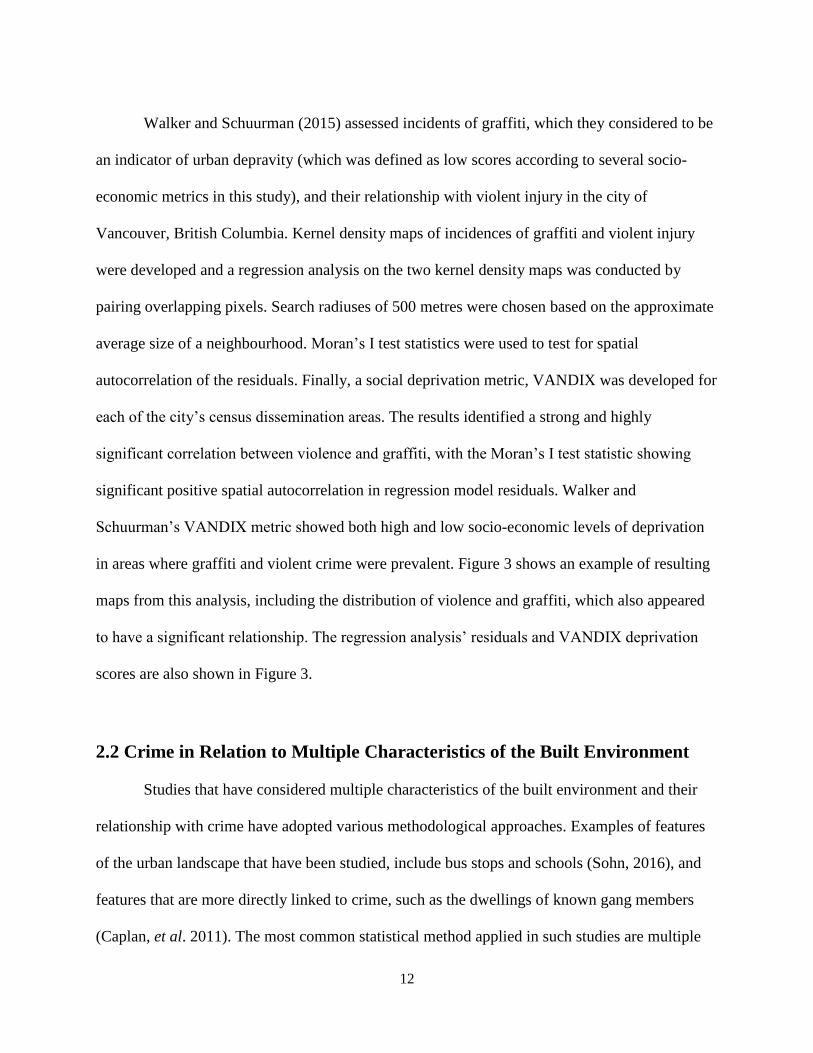
Figure 3. Kernel density maps of violent trauma and graffiti in Vancouver, British Columbia.
Residuals of a regression analysis are shown, along with urban deprivation scores by census
dissemination area (Walker & Schuurman, 2014, p. 7). ............................................................... 11
Figure 4. The kaleidoscope of urban features described by Barnum, et al., (2017). “A confluence
of certain features” altogether can “create conditions conducive to offending” (p. 205). ............ 14
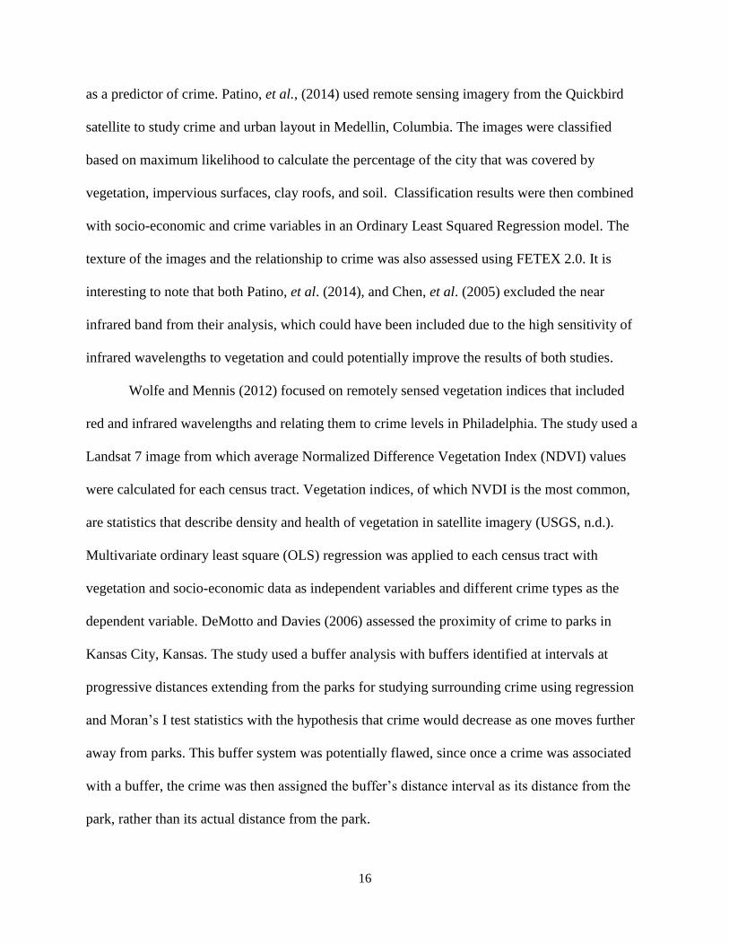
Figure 5. Maps of census tracts in Philadelphia showing mean NDVI and Aggravated Assault
per 1,000 people. Fewer aggravated assaults were observed in places with higher NDVI values
(Wolfe & Mennis, 2012, p. 116-117). .......................................................................................... 17
Figure 6. Conceptual diagram of the study’s research framework. Positive and negative effects
of built or natural environment features on crime and reported incidents are identified in this
diagram. These are hypothesised relationships within a theoretical framework and not based on
actual results of this study. ............................................................................................................ 19
Figure 7. Map of cities and townships of the Region of Waterloo, Ontario, Canada. Kitchener
and Waterloo are highlighted in yellow (Dodsworth, 2013). ....................................................... 24
Figure 8. A subset of a 2013 Landsat 8 satellite image showing the study area of the sister cities
of Kitchener and Waterloo, Ontario.............................................................................................. 25
Figure 9. A map of Waterloo and Kitchener, Ontario with important landmarks highlighted,
including each city’s downtown cores, major roads, major malls, and universities and colleges.
As previously shown in Figure 7, Waterloo is the northern city, while Kitchener is the southern
city................................................................................................................................................. 26
Figure 10. Overall crime rates (except traffic violations) reported in the Region of Waterloo,
Ontario compared to national crime rates in Canada from 2003 to 2013. Adopted from the 2013
WRPS annual report (WRPS, n.d.b). ............................................................................................ 27
Figure 11. A diagram demonstrating that for crime and reported incidents data collected by the
Waterloo Regional Police Service (WRPS), crime and reported incident points are moved from

ix
their original location (“address point” within the diagram) to the closest intersection node. Note
that in this example, the closest street intersection is chosen despite the fact that it is not actually
located on the street on which the address point is located. (Gloade, 2016; Brinon, 2016) ......... 31
Figure 12. A histogram of the distance between street intersections in Kitchener. Note that the x-
axis has been cut off at a maximum of 200 m. ............................................................................. 38
Figure 13. A diagram demonstrating the procedure of creating the 90 m and adaptive buffers. . 38
Figure 14. The buffers created using a 90 m radius (left) and adaptive method (right). Note that
buffers located partially outside the boundaries of Kitchener were not included in the study. .... 39
Figure 15. A simplified diagram showing the overall operation of the “Proportion Buffer Cutter”
....................................................................................................................................................... 40
Figure 16. The intersection of Highland Road and Patricia Avenue with its 90 m buffer (Buffer
ID 1730) and the various built environment features that comprise the independent variables
(expressed as percentages of each building type within the radius, as well as the number of
alcohol licenses, bus stops, and streetlights within the radius). .................................................... 42
Figure 17. A two dimensional demonstration of the KDE operation. The “x” marks on the x-axis
represent individual sample points, the curves above the points represent the curves applied on
top of each point, and the bolder line on top represents the surface of the KDE. Note how the
surface increases as the points get denser and as the surface gets closer to the centre of the points
in the clusters (Silverman, 2016, p. 14). ....................................................................................... 44
Figure 18. A histogram of the number of street intersections within each grid square within the
450 m by 450 m grid in Kitchener-Waterloo. Note that the x-axis does not include zero, by far
the most frequent value (328), in order to aid the interpretability of the rest of the histogram. ... 45
Figure 19. Steps involved with creating a 450m by 450m grid that assigned bandwidth values for
creating AKDE rasters. First, the number of number of intersections per zone was calculated, as
shown in the left map. Second, the number of intersections per kilometer was calculated, as
shown in the centre map. Third, the bandwidths for the zones were assigned based on the
intersections per kilometer in each, as shown in the right map. ................................................... 46
Figure 20. A diagram of the process involved in creating the AKDE rasters and extracting the
values using intersection points. ................................................................................................... 47
Figure 21. Examples of AKDE maps of GRT Bus Stops (left) and Alcohol Licensed Restaurants
(right). Major roads are indicated. ............................................................................................... 49

x
Figure 22. A diagram illustrating the process of preparing NDVI datasets from remote sensing
imagery. ........................................................................................................................................ 50
Figure 23. Maps showing street intersections in Kitchener with the percentage of building space
within 90 m buffers that is classified to be commercial (left) and residential (right). .................. 59

xi
List of Tables
Table 1. Primary study datasets and data sources for Kitchener-Waterloo ................................. 29
Table 2. A summary table of built and natural environment independent variables applied based
on buffer methodology, including how each variable was measured and areal coverage within the
City of Kitchener........................................................................................................................... 52
Table 3. A summary table of built and natural environment independent variables applied based
on buffer methodology, including how each variable was measured and the number of
occurrences within Kitchener-Waterloo. ...................................................................................... 54
Table 4. All independent variables included in OLS and logistic regression models of crime
reported incidents based on the 90 m and adaptive buffers, and the AKDE method. .................. 56
Table 5. Results of eight regression models tested in the analysis of NDVI and crime/reported
incidents. “***” represents a p-value below 0.001, “**” represents a p-value below 0.01 but
above 0.001, and “*” represents a p-value below 0.05 but above 0.01. ..................................... 105
Table A1. The results of the 90 m buffer OLS regression analysis in Kitchener. ..................... 130
Table A2. The results of the adaptive buffer OLS regression analysis in Kitchener. ................ 131
Table A3. The results of the 90 m buffer logistic regression analysis in Kitchener. ................. 132
Table A4. The results of the adaptive buffer logistic regression analysis in Kitchener. ............ 133
Table A5. The results of the AKDE OLS regression analysis in Kitchener-Waterloo. ............. 134
Table A6. The results of the AKDE logistic regression analysis in Kitchener-Waterloo. ......... 135

1
1.0 Introduction
In the study of geographical patterns of crime, the relationship between crime and the
built and natural environment has often been explored (Kumar & Waylor, 2003; Wolfe &
Mennis, 2012; Barnum et al., 2017). These studies usually focus on one specific characteristic of
the built or natural environment. Some studies examine built characteristics, such as alcohol
sales establishments or streetlights, and exploring their positive or negative effects on crime (Day
et al., 2012; Pain et al., 2006). There is also interest in studying the spatial relationship between
patterns of crime and the natural environment (Kuo & Sullivan, 2001b; Wolfe & Mennis, 2012).
There has been considerable debate about whether relationships between the natural environment
and crime rates are positive or negative. However, studies rarely take into account multiple
relationships between characteristics of the built and natural environment. This study attempts to
conduct a comprehensive assessment of the relationship between crime/reported incidents and
the built and natural environment by adopting a geospatial approach, which includes multiple
variables and datasets.
This study is conducted on the sister cities of Kitchener and Waterloo, Ontario. The focus
is on crime and reported incidents from the year 2013, with the locations of the crimes and
reported incidents aggregated to the nearest intersection due to privacy concerns. The study
examined 18 types of crime and reported incidents ranging from “assault” to “theft under
$5,000”. Built environment features taken into account include various building types (e.g.
residential buildings and commercial building), alcohol licensed establishments, and bus stops,
as well as more specific building types, such as churches and police stations. Natural
environment features were represented by parks or open space, as well as considering remote
sensing observations based on the Normalized Difference Vegetation Index (NDVI).

2
There were two main methods used to investigate the relationship between
crime/reported incidents and the built and natural environment. The first involved examining
crime and reported incidents in the city of Kitchener. Using ArcGIS and Python codes developed
for this study, circular buffers were specified around each street intersection in which built and
natural environment classes were identified. An OLS and logistic regression were conducted to
assess the strength of relationships between the built and natural environment and police
recorded crime and incidents using R programming. The second analysis involved creating
adaptive kernel density rasters (AKDE) of various built environment features in both Kitchener
and Waterloo. The intersections were then used to extract the values from the AKDE rasters that
intersected each intersection point. The relationship between the reported crime/reported
incidents and AKDE values at each intersection was then investigated, again using OLS and
logistic regression in R. An additional analysis used buffers to investigate the relationship
between NDVI values around each intersection and the crime and reported incidents at each
intersection. The goal of this study was to gain a better understanding of the relationship between
the built and natural environment and to contribute to existing literature on this topic. This study
adopted an inductive approach when exploring relationships between the built and natural
environment and crime, since some hypothesised effects were deduced from existing literature,
while other relationships between crime and environmental features were theorized based on this
study’s findings.
1.1 Problem Statement
The goal of this study is to explore the relationship between features of the built and
natural environment and crime/reported incidents in the cities of Kitchener and Waterloo,

3
Ontario. The first objective of this study is to investigate the link between the level of
crime/reported incidents and the built environment in the Kitchener-Waterloo area using GIS
datasets. The intention is to build upon the studies such as those conducted by Kumar and
Waylor (2003) and Day et al. (2012), which found a strong relationship between liquor stores
and alcohol serving establishments and crime rates, as well as studies such as those by Barnum et
al. (2017) and Sohn (2016) who investigated the built environment/crime relationship in a more
comprehensive manner. By adopting a holistic and comprehensive approach in this study, other
built features were included in the analysis and statistical methods were adopted for identifying
significant relationships with criminal activity.
The second objective of this study is to investigate the link between levels of
crime/reported incidents and the natural environment in Kitchener-Waterloo using GIS and
remote sensing data. Findings are then compared with previous studies such as those by Wolfe
and Mennis (2012) and Chen, et al., (2005), which both found a strong negative relationship
between crime and vegetation cover. Finally, the third objective of this study is to identify which
built and natural environment features have the strongest relationships with different crime and
reported incident types in the Kitchener-Waterloo region by adopting an exploratory spatial data
analysis approach.
1.2 Thesis Structure
The thesis is composed of nine sections:
Chapter 1 – Introduction: Establishes the topic of the thesis, while also explaining the basics of
the thesis’ methodological setup.

4
Chapter 2 –Literature Review: Outlines the popular theories that are commonly discussed in
previous studies of the relationship between the built and natural environment. It also discusses
the methods and conclusions of previous studies on this topic.
Chapter 3 – Conceptual Framework: Establishes the concept structure that the ideas of thesis
are based upon. It also discusses the literature contained similar concepts, many of which were
sources of inspiration for this study’s conceptual framework.
Chapter 4 – Study Area: Discusses the region in which this study was performed, including
relevant statistics and characteristics.
Chapter 5 – Data: Discusses the many datasets used in this study, while also discussing any
data processing needed to improve these dataset.
Chapter 6 – Method: Outlines in detail the methodologies implemented in this study and
outlines the statistics and datasets used with each.
Chapter 7 – Results: Analyses the results of each model estimated for the study, while also
examining the independent variables tested in each.
Chapter 8 – Discussion: Discusses overarching findings of the study, while also discussing its
weaknesses and comparing those findings to the literature reviewed earlier.
Chapter 9 – Conclusions: Concludes the findings of the study while discussing its implications
on future work.

5
2.0 Literature Review
Crime can be linked to the location at which it occurs. According to Routine Activity
Theory (Cohen & Felson, 1979), crime rates in a particular time and space can be influenced by
three factors: motivated offenders, suitable targets, and the lack of capable guardians (Figure 1).
The theory argues that the convergence of suitable targets and the lack of guardianship at a
particular time and space will increase crime rates at that particular time and space. In later
writings, Felson (1987) discussed how various “facilities”, such as shopping centres,
condominium complexes, office buildings, and schools, make up an urban framework, which he
called the “metroquilt”. Felson states that there is an imbalance in crime risk with some areas of
this “metroquilt” having a greater risk of crime than others due to such facilities. He exemplified
this by demonstrating that residential and retail facilities account for 22% and 19% of property
crime, respectively, in Chicago during 1984.
Brantingham and Brantingham’s 1995 study entitled, “Criminality of place: Crime
generators and crime attractors” is often cited in environmental criminology literature, which
puts forward the concepts of “crime generators” and “crime attractors”. “Crime generators” are
places where many people congregate, such as a shopping mall, which presents criminal
opportunities for a potential offender who might not have otherwise committed a crime. “Crime
attractors” are places that present criminal opportunities for offenders with the intent to commit a
specific crime. According to the authors, a city’s environment “urban backcloth” can have a
great influence on the quantity and types of crimes committed, as well as the time at which they
are committed.

6
Figure 1. A Venn diagram of Cohen and Felson’s (1979) Routine Activity Theory showing
crime and delinquency as a product of the intersection of motivated offenders, lack of capable
guardians, and suitable targets. Adapted from Siegel and Worrall (2015).
Previous research has also supported a relationship between crime and surrounding
vegetation cover (Wolfe & Mennis, 2012; Chen, et al., 2005; DeMotto & Davies, 2006),
although the direction of this relationship is debated. Some studies suggest that vegetation cover
increases the incidence of crime, but these studies often tend to focus on the fear of crime as
opposed to actual crime (e.g. people fearing that trees and other large plants could be used as
hiding places for people intent on committing crimes against them) or base their findings on
accounts of offenders using vegetation in hiding their criminal activities (Nasar & Fisher, 1993;
Michael, et al., 2001). The idea of unkempt and overgrown vegetation increasing the level of
Motivated offenders
•Teenage males
•Unemployed persons
•Drug abusers
•Unsupervised youths
•Gang members
Suitable targets
•Unguarded homes
•Unlocked cars
•Unprotected stores
•Unmarked items
Lack of capable guardians
•Homeowners
•Police
•Neighbourhood watch groups
•Security guards
•Parents
CRIME
&
DELINQUENCY

7
crime is consistent with the “broken window theory” proposed by Kelling and Wilson (1982),
which states that disorder in the physical environment can make a location prone to criminal
invasion. Others have suggested that vegetation decreases levels of crime or that a lack of
vegetation tends to increase crime levels (Wolfe & Mennis, 2012; Chen, et al., 2005).
Two main reasons have been put forward to explain why vegetation may have a negative
effect on criminal activity. First higher surveillance may result from more individuals using
greenspace areas (Kuo and Sullivan, 2001b), thus deterring criminal activity. Second, the
presence of vegetation may result in positive psychological effects by alleviating mental fatigue
and reducing deviant behaviour (Kaplan, 1987). Increased surveillance due to people using
greenspaces and associated reduction in crime is consistent with the ideas presented by Jacobs
(1961) in her publication, “The Death and Life of Great American Cities” where she states that
more “eyes upon the street” help to increase surveillance and therefore keep the streets safe (she
also noted, however, that greenspaces must have a “diversity of uses and users” to enliven a
neighbourhood or it might simply further depress an area) (p. 35, 111). This is further supported
by Kuo and Sullivan (2001b), who found that both property and violent crime were lower in
apartment complexes located in close proximity to open and vegetated spaces than those that
were not. The authors partially attributed this to increased surveillance (i.e. recreational uses,
passersby) due to vegetation and greenspaces. A decrease in mental fatigue due to vegetation is
supported by Kaplan (1987), who stated that mental fatigue can increase violent behaviour in
individuals. He defines mental fatigue as “a state of discomfort and reduced effectiveness that
usually follows intense mental effort” (p. 56). Kaplan (1987) suggested that parks and gardens
can help alleviate mental fatigue in an urban setting. This theory is supported by Kuo and
Sullivan (2001a), who found that residents in public housing reported fewer incidents of violence

8
and/or aggression in building complexes with higher amounts of vegetation than at building
complexes with a lower presence of vegetation.
An environmental approach is often adopted only as a partial explanation for the locality
of crime. This approach tends to explain or at least partially explain the geographic distribution
of crime according to socioeconomic factors, such as household income, employment and
demographics (Ackerman & Murray, 2004; Ceccato & Dolmen, 2011). Some studies account for
socio-economic factors in their analyses as a control variable (Wolfe & Mennis, 2012; Sohn,
2016). However, other studies do not account for socio-economic factors and instead focus on
the direct link between crime and the environment, both built and natural (Kumar & Waylor,
2003; Piza et al., 2013; Barnum et al., 2017).
2.1 Crime in Proximity to Single Characteristics of the Built Environment
The relationships between single characteristics of the built environment and crime were
often examined using similar methods (Pain et al., 2006; Kumar & Waylor, 2003; Suresh &
Vito, 2009). The most common environment features studied within the literature were the
presence of bars, liquor stores, and other sources of alcohol sale (Day et al., 2012; Kumar &
Walyor, 2003). Many other built environment features and their relationship with crime have
been an object of study, ranging from government subsidized housing to streetlights (Suresh &
Vito, 2009; Pain, et al., 2006). Common methods applied in these studies are regression
techniques (Day, et al., 2012; Kumar & Walyor, 2003; Suresh & Vito, 2009; Walker &
Schuurman, 2015) and Moran’s I test statistics for spatial autocorrelation (Suresh & Vito, 2009;
Walker & Schuurman, 2015). Results from these studies have supported strong relationships
existing between crime and various features of the built environment.

9
Day, et al. (2012) examined how crime is affected by the accessibility of alcohol outlets
in different regions of New Zealand. This study assessed the median distance to alcohol outlets
in police station areas, which involved using census mess-blocks and comparing corresponding
violent crime rates in the police station area, while controlling for demographic variables (2012).
Statistical analysis was based on a negative binomial regression. The results suggested that
geographic access to alcohol establishments can serve as a significant predictor when studying
violent crime, and the two form a negative relationship where violent crime increases as median
distance to alcohol outlets decreases. Kumar and Waylor (2003) also examined the proximity of
crime incidents to alcohol facilities in Savannah, Georgia. A logistic regression model was used
to assess the probability of crime at various intervals of proximity to places of alcohol services.
A map of Savannah showing crimes and alcohol services in 2000 is shown in Figure 2. In
contrast to Day, et al. (2012), Kumar and Waylor (2003) did not control for demographic
variables. However, both studies arrived at similar findings, identifying higher crime density in
areas in close proximity to alcohol establishments.
Similar studies include Pain, et al., (2006) who assessed streetlighting and its relation to
crime and fear of crime in several towns in Northumberland, England. This study involved a two
pronged analysis. First, a GIS approach was adopted to compare crime hotspots and streetlight
coverage to identify areas that experienced high incidents of crime and low streetlight coverage.
The second part of the study involved conducting interviews in the ten most problematic areas of
the city, as a means of qualitative rapid community appraisal. The results noted that crime
hotspots and the residents’ views of high crime locations did not necessarily match, partly due to
unreported crime. Overall, most surveyed residents did not believe that improvements in

10
streetlighting in their area would have a significant impact on levels of crime, although improved
streetlighting could potentially reduce the overall fear of crime.
Figure 2. A map showing alcohol services (the large dots) and crime locations (the small dots) in
Savannah, Georgia in 2000 from Kumar and Waylor (2003).
Suresh and Vito (2009) evaluated the relationship between public housing and homicide
in Louisville, Kentucky. This study involved creating 1,000 foot buffers around public housing
projects in the city and then using buffers to assess the distribution of crime in the city. A spatial
regression was then conducted on homicides in the city between 1989 and 2007. The results

11
showed that public housing had a significant effect on the spatial distribution of homicides in
Louisville. When new public housing arose in mixed-income communities, the homicide clusters
appeared to be displaced to other low-income areas. A spatial regression analysis determined that
both median income of residents and vacant housing were both significant predictors of
homicide.
Figure 3. Kernel density maps of violent trauma and graffiti in Vancouver, British Columbia.
Residuals of a regression analysis are shown, along with urban deprivation scores by census
dissemination area (Walker & Schuurman, 2014, p. 7).
12
Walker and Schuurman (2015) assessed incidents of graffiti, which they considered to be
an indicator of urban depravity (which was defined as low scores according to several socio-
economic metrics in this study), and their relationship with violent injury in the city of
Vancouver, British Columbia. Kernel density maps of incidences of graffiti and violent injury
were developed and a regression analysis on the two kernel density maps was conducted by
pairing overlapping pixels. Search radiuses of 500 metres were chosen based on the approximate
average size of a neighbourhood. Moran’s I test statistics were used to test for spatial
autocorrelation of the residuals. Finally, a social deprivation metric, VANDIX was developed for
each of the city’s census dissemination areas. The results identified a strong and highly
significant correlation between violence and graffiti, with the Moran’s I test statistic showing
significant positive spatial autocorrelation in regression model residuals. Walker and
Schuurman’s VANDIX metric showed both high and low socio-economic levels of deprivation
in areas where graffiti and violent crime were prevalent. Figure 3 shows an example of resulting
maps from this analysis, including the distribution of violence and graffiti, which also appeared
to have a significant relationship. The regression analysis’ residuals and VANDIX deprivation
scores are also shown in Figure 3.
2.2 Crime in Relation to Multiple Characteristics of the Built Environment
Studies that have considered multiple characteristics of the built environment and their
relationship with crime have adopted various methodological approaches. Examples of features
of the urban landscape that have been studied, include bus stops and schools (Sohn, 2016), and
features that are more directly linked to crime, such as the dwellings of known gang members
(Caplan, et al. 2011). The most common statistical method applied in such studies are multiple

13
regression modelling (Sohn, 2016; Piza, et al., 2014). Barnum et al. (2017) and Caplan et al.
(2011) and a technique called risk terrain modelling (RTM).
Caplan et al. (2011) examined crime hotspots in Irvington, New Jersey using RTM as a
place-based forecasting method. They used RTM to create raster maps that demonstrated risk
level using three variables considered to be predictors of shootings, namely dwellings of known
gang members, drug arrest locations, and retail business locations, and tested these maps against
other types of crimes. Sohn (2016) tested the practicality of ‘crime prevention through
environmental design’ in Seattle by analysing crime and various built environment features. This
study used residential crime density in neighbourhoods defined by 500 m buffers, which was
included in a regression analysis, along with population density, building height, road density,
ratio of commercial buildings to residential buildings, bus stop density, intersection density, and
ratio of park area to residential area.
Barnum et al. (2017) compared a diverse group of built environment features, ranging
from foreclosed homes to schools to bus stops to bars whose arrangement they described as a
“kaleidoscope” of urban features (see Figure 4). This study used RTM to compare effects of
various urban features on risk of robbery in Chicago, Kansas City, and Newark. Piza et al.
(2014) attempted to assess which CCTV camera locations yielded a reduction in crime, and tried
to explain the varying effects of CCTV cameras on spatial patterns of crime. These assessments
focused on how crime at locations with cameras (before and after they were installed) were
associated with, (a) environmental features such as bars and transit stops, (b) line of sight
variables such as percentage of foliage obstruction, (c) enforcement variables such as crime
detections from the CCTV cameras, and (d) a variable indicating the type of CCTV camera in
use.

14
Figure 4. The kaleidoscope of urban features described by Barnum, et al., (2017). “A confluence
of certain features” altogether can “create conditions conducive to offending” (p. 205).
Conflicting findings are often reported on the effect of built environment features (e.g.,
bus stops) on levels of crime in urban environments (Sohn, 2016; Barnum et al., 2017). Barnum
et al. (2017) also emphasized that the effect on crime by place features can vary greatly from city
to city. Caplan et al. (2011) found that RTM was more accurate in predicting future shootings
than retrospective hotspot mapping. Sohn (2016) found that the variables they considered, except
for average building high and population density, had a negative effect on crime. Notably, bus
stops were determined to have a negative relationship with crime. Barnum et al. (2017) found
that foreclosed homes, gas stations, bus stops, grocery stores, liquor stores, and drug markets
were all consistent risk factors for robbery in all three cities that were included in their study.
However, other factors, such as parks, bars, and schools were not risk factors in all of the cities.
Piza et al. (2014) found that decreases in overall crime, violent crime, and theft from autos were
significantly associated with camera enforcement. Decreases in violent crime and robbery were

15
significantly associated with viewsheds containing bars. Violent crime, robbery, and theft from
automobiles were lower where percentage coverage of camera image by immovable objects was
high.
2.3 Crime and the Natural Environment
Many studies have examined the relationship between the natural environment and crime
using different data sources and methodologies. Remote sensing has been applied, making use of
the technique’s ability to measure an entire study area, although their methods of using the
imagery varied widely (Chen, et al., 2005; Patino, et al., 2014; Wolfe & Mennis, 2012). Other
studies have focused on parkland and other vegetation covered areas (DeMotto & Davies, 2006;
Sohn, 2016; Barnum, et al., 2017). Some research has focused on comparing the relationship
between vegetated areas and crime rates versus that of non-vegetated areas (Chen, et al., 2005;
Wolfe & Mennis, 2012). Some studies have examined vegetation alone in its relationship with
crime (DeMotto & Davies, 2006; Wolfe & Mennis, 2012), while others have considered
confounding effects of other urban environment features such as bus stops and foreclosed homes
(Patino, et al., 2014; Sohn, 2016; Barnum, et al., 2017).
Chen, et al., (2005) used both remote sensing and GIS to study the relationship between
crime and vegetation in Carlsbad, California. This study obtained high resolution PAN images
taken from SPOT, and images were classified using the ISODATA clustering method and a 300
m grid, which identified two classes (vegetation and non-vegetation). The study involved three
steps of analysis, including spatial clustering of crime and assessing where those clusters
occurred, a traditional regression analysis that attempted to explain crime according to variables
of propensity and opportunity, and a spatial filtered regression analysis to study spatial clustering
16
as a predictor of crime. Patino, et al., (2014) used remote sensing imagery from the Quickbird
satellite to study crime and urban layout in Medellin, Columbia. The images were classified
based on maximum likelihood to calculate the percentage of the city that was covered by
vegetation, impervious surfaces, clay roofs, and soil. Classification results were then combined
with socio-economic and crime variables in an Ordinary Least Squared Regression model. The
texture of the images and the relationship to crime was also assessed using FETEX 2.0. It is
interesting to note that both Patino, et al. (2014), and Chen, et al. (2005) excluded the near
infrared band from their analysis, which could have been included due to the high sensitivity of
infrared wavelengths to vegetation and could potentially improve the results of both studies.
Wolfe and Mennis (2012) focused on remotely sensed vegetation indices that included
red and infrared wavelengths and relating them to crime levels in Philadelphia. The study used a
Landsat 7 image from which average Normalized Difference Vegetation Index (NDVI) values
were calculated for each census tract. Vegetation indices, of which NVDI is the most common,
are statistics that describe density and health of vegetation in satellite imagery (USGS, n.d.).
Multivariate ordinary least square (OLS) regression was applied to each census tract with
vegetation and socio-economic data as independent variables and different crime types as the
dependent variable. DeMotto and Davies (2006) assessed the proximity of crime to parks in
Kansas City, Kansas. The study used a buffer analysis with buffers identified at intervals at
progressive distances extending from the parks for studying surrounding crime using regression
and Moran’s I test statistics with the hypothesis that crime would decrease as one moves further
away from parks. This buffer system was potentially flawed, since once a crime was associated
with a buffer, the crime was then assigned the buffer’s distance interval as its distance from the
park, rather than its actual distance from the park.

17
Figure 5. Maps of census tracts in Philadelphia showing mean NDVI and Aggravated Assault
per 1,000 people. Fewer aggravated assaults were observed in places with higher NDVI values
(Wolfe & Mennis, 2012, p. 116-117).
The relationship between vegetation and crime has conflicting results in the literature.
While many studies have identified lower crime rates in the presence of vegetation (or lack of
vegetation increasing levels of crime) (e.g., Wolfe & Mennis, 2012; Chen, et al., 2005), other
research have associated higher crime levels with vegetation cover (e.g., DeMotto & Davies,
2006), while some failed to find any significant relationship between the two variables (e.g.,
Patino, et al., 2014). In particular, Chen, et al., (2005) found that areas of highest crime rates
were associated with shopping centres and commercial areas. A cluster analysis revealed that
burglaries and assault were most associated with non-vegetated grid cells. The authors concluded
that the classification of satellite imagery into a non-vegetation index was successfully applied
for predicting where burglary hotspots were geographically located. Patino, et al., (2014) found
that the best performing remotely sensed variable was percentage of other impervious surfaces

18
(i.e., impervious surfaces that are not clay roofs), where average homicide rates tended to be
higher where more impervious surfaces were present. Unlike findings from other studies, the
authors found percentage of vegetation to be an insignificant predictor. Wolfe and Mennis (2012)
found that almost all types of crime were both negatively and significantly associated with
vegetation, meaning that crime decreased as the amount of vegetation increased. This
relationship between crime and vegetation was independent of the socio-economic status of
neighbourhoods. Figure 5 shows maps of average NDVI values and aggravated assault per 1,000
persons in each Philadelphia census tract, where the relationship between both variables was
significant. In contrast, DeMotto and Davies (2006) determined that levels of crime tended to
increase as distance to parkland decreased.
Such conflicting findings between research studies on the links between crime and
features of the built and natural environment highlight that such relationships are complex and
likely differ based on their geographical, demographic, and socioeconomic context. This
suggests that further research is required, especially adopting a more holistic and comprehensive
approach exploring links between multiple characteristics of the built and natural environment
and crime, rather than single attributes at a time.

19
3.0 Conceptual Framework
Figure 6. Conceptual diagram of the study’s research framework. Positive and negative effects
of built or natural environment features on crime and reported incidents are identified in this
diagram. These are hypothesised relationships within a theoretical framework and not based on
actual results of this study.
The conceptual framework of this study is based on the hypothesis that features of the
built and natural environment affect the location of where incidents of crime may be reported. In
turn, these reports of crime affect the location of police activity. The built environment refers to
man-made physical features of the urban environment being studied, such as shopping centres,
bus stops, or houses, with the function of each building or object being important to its
classification. The natural environment consists of features within the urban environment studied
that are natural, such as occurrence of vegetation and water bodies. The natural environment can

20
also refer to natural features that are planned, such as parks and ponds. Figure 6 shows the
relationship between these features and their potential effects on crime and reported incidents.
The influences shown in the diagram can work in multiple pathways and directions depending on
the type of crime committed. In some situations, a criminal might commit a crime in a certain
area due to the characteristics of its environment. For example, a thief may target a bus stop,
since it is a place where people often congregate outdoors, thus creating an opportunity for theft,
according to Routine Activity Theory (Cohen & Felson, 1979). Other crimes may occur due to a
location influencing the actions of the criminal and may be a partial cause for committing the
crime. Examples may include public intoxication or assault near a bar. While the person likely
did not go to a bar intending to commit a crime, the environment may influence the individual to
commit a crime, namely due to intoxication from consuming alcohol at the bar.
Consequently, an environmental setting can both influence where a criminal commits a
crime and influence an individual to commit a crime. This is consistent with Brantingham and
Brantingham’s 1995 paper, which described the concept of “crime attractors” and “crime
generators”. “Crime generators” create opportunities to commit crime due to the large
concentration of people at a location that potential criminals might exploit. “Crime attractors”
tend to attract people with the intent of committing a particular crime given the opportunities
presented at that location (Brantingham and Brantingham, 1995).
In addition to creating opportunity and influencing criminals to commit crime,
environmental features also have the potential to serve as crime deterrents. For example, a
criminal may not want to commit a crime near a streetlight during night time due to the greater
likelihood of being seen. Another example from the literature is Piza, et al. (2014), who

21
concluded that a CCTV camera can have a deterrent effect when installed in a proper manner and
setting.
In the case of crime attractors, influences or deterrents to crime included in this study
comprised of three categories of the built environment, including types of buildings, bus stops,
and streetlights. Within the built environment, as previously discussed and in accordance with
Routine Activity Theory, bus stops were hypothesised to have a positive effect on crime within
their vicinity, meaning that high levels of crime within their vicinity would be expected.
Streetlights were expected to have a negative effect on crime, resulting in lower levels of crime
relative to other unlit or dark areas during night hours.
The building types considered in this study included residential, educational, religious,
commercial, recreational, institutional, agricultural, industrial, and alcohol serving or sales
establishments. Alcohol serving/selling establishments were expected to have a positive effect on
crime, since the consumption of alcohol can often promote irrational or deviant behaviour that
may result in criminal offences (Day, et al. 2012; Livingston, 2007; Kumar & Waylor, 2003).
Other buildings, such as educational and religious facilities were expected to have a negative
effect on crime due to the concentrated presence and congregation of children and the elderly,
who were expected to behave as crime deterrents. Other buildings, such as industrial buildings,
did not have a hypothesised effect on crime as they were not addressed in the reviewed literature.
In this way, this study adopts an inductive approach to the research.
All natural environmental factors, including the presence of parks and general vegetation
cover, were expected to have a negative effect on crime. As previously discussed, there is
frequent debate within the literature as to whether the presence of vegetation cover has a positive
or negative effect on crime. Some studies support the notion that increased vegetation cover

22
results in a rise in criminal activity by increasing the number of potential hiding spots for
criminals and their criminal activities (Michael, et al., 2001). Others suggest that increased
vegetation cover results in a negative effect on crime, since it causes more people to be present
outdoors, allowing for increased surveillance and also because vegetation promotes
“psychological softening” and alleviates stress (Wolfe & Mennis, 2012). This research adopts the
hypothesis of more recent studies, including Wolfe and Mennis (2012) and Chen, et al. (2005),
which suggest that less crime results in areas with higher vegetation cover and more crime
occurs in areas of scarce vegetation cover.

23
4.0 Study Area
The study area includes the cities of Kitchener and Waterloo in Ontario, Canada with a
map shown in Figure 7 and a satellite photo shown in Figure 8. The two cities are also shown in
Figure 9, which displays major landmarks and roads. The cities are located in Southwest Ontario
and are located in the larger Region of Waterloo (Region of Waterloo, 2011). The Region of
Waterloo is policed by the Waterloo Regional Police Service (WRPS). Both cities contain mostly
urban land, although there is some rural area included within each city’s boundary. The city of
Waterloo has a population of 98,780 according to the 2011 census and is the 52nd largest
municipality in Canada (Statistics Canada, 2016b). It is known as a university town, being home
to the University of Waterloo and Wilfred Laurier University, as well as a satellite campus of
Kitchener’s Conestoga College. It is also known as a high tech centre and is home to companies
such as Blackberry (English, 2011). The city of Kitchener is located directly south of the city of
Waterloo. It is the largest city in the Waterloo Region with a population of 219,153 in the 2011
census and is the 22nd largest municipality in Canada (Statistics Canada, 2016b). Kitchener’s
economy is considered to be more “blue-collar” than that of Waterloo and the city has
experienced the type of urban decline that is often associated with North American industrial
centres in the past 50 years (English, 2011). However, the city has experienced much urban
redevelopment in the past two decades and has more recently become host to a number of high-
tech companies (English, 2011). Together, along with Cambridge, Woolwich, and North
Dumfries, the two cities help form a Census Metropolitan Area (CMA) called “Kitchener -
Cambridge - Waterloo, Ontario”, which is the 4th largest in Ontario and the 10th largest in Canada
(Statistics Canada, 2016a).

24
Figure 7. Map of cities and townships of the Region of Waterloo, Ontario, Canada. Kitchener
and Waterloo are highlighted in yellow (Dodsworth, 2013).
The Region of Waterloo is a relatively safe place in terms of criminal activity and crime
rates. In a ranking of the most dangerous cities in Canada by Maclean’s magazine in 2010,
Kitchener ranked as the 65th most dangerous city in Canada with a crime score that was 15.88%
lower than the country’s overall crime score (Maclean’s, 2010). As shown in Figure 10 from the
WRPS 2013 annual report, the overall crime rate has been on a decreasing trend in the Region of
Waterloo over the decade leading up to 2013, which is the year of crime and reported incident
data used in this study. The violent crimes rate (not shown in Figure 10) had previously been on
an increasing trend from 2003 to 2010, but the rate decreased between 2010 and 2013 (WRPS,
n.d.b). The overall crime rate for the Region of Waterloo was well below Canada’s overall crime
rate from 2003 to 2013, but was somewhat higher than Ontario’s overall crime rate from 2009 to
2013 (WRPS, n.d.b).

25
Figure 8. A subset of a 2013 Landsat 8 satellite image showing the study area of the sister cities
of Kitchener and Waterloo, Ontario.
Despite Kitchener-Waterloo being classified as a relatively safe city, it was still
nevertheless chosen as the study area for this thesis for several reasons. The first reason being
that this study was conducted at the University of Waterloo, resulting in inherent interest in
studying the local region, ease of access to the study area for ground truth and data verification,
and potential contacts with the WRPS and local experts. This also allowed for greater user
familiarity with the study area and application of local knowledge during both development and
analysis phases of the study. There may also be wider relevance and potential application of
study results compared to conducting the study elsewhere on an arbitrarily selected or less
familiar locality. The second reason was that a smaller study area may allow for a more
manageable and definable study, resulting in more focus on the urban environment and crime

26
relationship with fewer confounding factors, which may be more prominent in larger
metropolitan areas. The third and perhaps most significant reason for selecting Kitchener-
Waterloo as the study area was the availability of high quality crime and reported incident data,
which was available as point dataset for the region.
Figure 9. A map of Waterloo and Kitchener, Ontario with important landmarks highlighted,
including each city’s downtown cores, major roads, major malls, and universities and colleges.
As previously shown in Figure 7, Waterloo is the northern city, while Kitchener is the southern
city.

27
Figure 10. Overall crime rates (except traffic violations) reported in the Region of Waterloo,
Ontario compared to national crime rates in Canada from 2003 to 2013. Adopted from the 2013
WRPS annual report (WRPS, n.d.b).

28
5.0 Data
Several geospatial datasets were used for this study, which were acquired from a variety
of sources, mainly from official government agencies. Formats include vector data, satellite
imagery, and simple spreadsheets, which often required significant processing prior to analysis.
For example, spreadsheet datasets were converted into vector point datasets and geocoded. A
summary of all datasets used in this study is provided in Table 1.
The principal dataset used in this study was crime and reported incident data collected by
the Waterloo Regional Police Service (WRPS). The available dataset contains points
corresponding to what the WRPS refers to as “occurrences”, which denotes a record of each time
police services were called (WRPS, 2015a). Therefore, these calls to service “do not represent
actual criminal activity”, since not all police calls involve crime (WRPS, 2015a, p. 2).
Occurrences considered to be criminal in nature are considered to be “police-reported crime” as
opposed to actual crime which requires a criminal conviction (WRPS, 2015a). Actual geographic
criminal conviction data would be difficult to obtain given the often lengthy processes of the
court system and confidentiality issues. Therefore, police-reported crimes within the dataset can
be considered to be a pseudo representation of criminal activity. Within this thesis, such
occurrences are referred to as “crime and reported incidents” or “crime/reported incidents”.

29
Table 1. Primary study datasets and data sources for Kitchener-Waterloo Subject Dataset Name Date
Created
Notes Source
Crime and
Reported
Incidents
WRPS Occurrence
Data
2013 All crime and reported incidents in the Waterloo Region in the year 2013. Also available for 2011 to 2015
Contains coordinates. Each point is located at the nearest
intersection
Contains both the purpose of the original call and what the crime (or other incident) was determined to have occurred
after the call was resolved
Waterloo Regional
Police Service
Building
Footprints
City of Kitchener
Buildings
Updated
regularly Contains the building footprints for all buildings in the city
of Kitchener
Also has a category to classify each buildings’ type
City of Kitchener
Bus Stops Transit - GRT Stops Updated regularly
Contains locations of all bus stops in the Waterloo Region used by Grand River Transit (GRT)
Region of Waterloo
Satellite
Imagery
Landsat 8 Satellite
Data
Sept. 17,
2013 Obtained from the USGS Global Visualization Viewer
website
Landsat 8 data
Covers entire Region of Waterloo
USGS
Roads Ontario Road
Network: Road Net
Element
2015 Contains all roads in Ontario
Used in this study to create street intersection data
Government of
Ontario
Police Stations Police Stations in
the Region of
Waterloo
2015 Waterloo Regional Police Service (WRPS) station
Locations obtained from police department website
Both Kitchener and Waterloo included
Waterloo Regional
Police Service
website
Liquor
Servicing
Establishments
Licensed
Restaurants
2014 A combination of information from Alcohol and Gaming Commission of Ontario and the City of Kitchener
Added to the footprint data
While City of Kitchener data only has the licensed restaurants in Kitchener, the Alcohol and Gaming
Commission of Ontario contains information for both
Kitchener and Waterloo
Alcohol and Gaming
Commission of
Ontario and City of
Kitchener
Municipal
Boundaries
City Town Village
Boundaries
Used for the boundaries of Kitchener and Waterloo for data clipping and various processes
Region of Waterloo
Streetlights Streetlight in the
City of Kitchener
Streetlights only for Kitchener City of Kitchener via
the UW Geospatial
Centre
Parks City of Kitchener
Parks
Updated
regularly Combined with golf courses to create greenspace data City of Kitchener
Golf Courses City of Kitchener
Golf Courses
Updated
regularly Combined with parks to create greenspace data City of Kitchener
Liquor Stores LCBO and Beer
Store in Kitchener and Waterloo
2015 Address of each LCBO and Beer Store in Kitchener and Waterloo were added
LCBO and Beer
Store website
Elementary
Schools
Elementary schools
in Kitchener and
Waterloo
Updated
regularly A combination of select data (only elementary schools)
from two datasets, from the City of Kitchener and the City
of Waterloo
City of Kitchener and
City of Waterloo
Secondary
Schools
Secondary Schools
in Kitchener and Waterloo
Updated
regularly A combination of select data (only secondary schools)
from two datasets, from the City of Kitchener and the City
of Waterloo
City of Kitchener and
City of Waterloo
Universities Universities and
Colleges in
Kitchener and
Waterloo
Updated
regularly A combination of select data (only post-secondary
institutions) from two datasets, from the City of Kitchener
and the City of Waterloo
Included colleges but not carrier colleges
Satellite campuses that occupied the same building were
counted as one campus
City of Kitchener and
the City of Waterloo
Hospitals Hospitals in
Kitchener and
Waterloo
Updated
regularly Since no hospitals are located in Waterloo, only the
Kitchener dataset was required
City of Kitchener
Places of Worship
Places of Worship in Kitchener and
Waterloo
Updated regularly
Combined datasets from Waterloo and Kitchener City of Waterloo and City of Kitchener
Libraries Libraries in
Kitchener and
Waterloo
Updated
regularly Combination of a shapefile dataset from City of Kitchener
and a shapefile created from address data from City of
Waterloo websites
City of Waterloo and
City of Kitchener
Community Centres
Community Centres in Kitchener and
Waterloo
Updated regularly
Combination of a shapefile dataset from City of Kitchener and a shapefile created from address data from City of
Waterloo websites
City of Waterloo and City of Kitchener
Arenas Arenas in Kitchener
Waterloo
Updated
regularly Combination of a shapefile dataset from City of Kitchener
and a shapefile created from address data from City of
Waterloo websites
City of Waterloo and
City of Kitchener

30
The dataset used for this study contains crime and reported incident records for the year
2013 (WRPS, 2015b). Each record contains several types of information, such as the reported
date and time, the priority level of the call, and the total time it took to resolve the situation
(WRPS, 2015a). The information considered to be most important for this study were the
“Geographic Location” and the “Final Call Type Description” (WRPS, 2015a). The “Geographic
Location” data column contains the x and y coordinate of the nearest intersection to each crime
and reported incident in the NAD1983 UTM Zone 17N Transverse Mercator projection
coordinate system (WRPS, 2015a). The reason for the location of each crime and reported
incident to be moved to the nearest street intersection is for protecting the privacy of callers and
victims involved (WRPS, 2015a). The diagram in Figure 11 demonstrates how crime and
reported incidents are assigned to the nearest street intersection. As shown in the diagram, the
nearest intersection is always chosen regardless of whether or not the intersection is located on
the same street as the crime or reported incident. “Final Call Type Description” denotes the
crime type attributed to each crime or reported incident after the call has been resolved (WRPS,
2015a). The data is provided in a spreadsheet format and therefore must be imported into
ArcCatalog as a Feature Class before it can be analysed spatially and statistically. All crime and
reported incidents missing geographic location or final call type information were eliminated
from the dataset. Also sourced from the WRPS website were the locations of police stations
(WRPS, n.d.a). A dataset was created using the address information of the police stations based
on Google Earth.

31
Figure 11. A diagram demonstrating that for crime and reported incidents data collected by the
Waterloo Regional Police Service (WRPS), crime and reported incident points are moved from
their original location (“address point” within the diagram) to the closest intersection node. Note
that in this example, the closest street intersection is chosen despite the fact that it is not actually
located on the street on which the address point is located. (Gloade, 2016; Brinon, 2016)
Several datasets were collected from the City of Kitchener’s open data catalogue. A key
dataset for this study was building footprints within the city, which were created using building
surveys, site plans, or aerial imagery (City of Kitchener, n.d.a). The building type in this study
was determined using the “CATEGORY” column of the dataset, which included:
“RESIDENTIAL”, “RECREATIONAL”, “INSTITUTIONAL”, “COMMERCIAL”,
“INDUSTRIAL”, “UTILITY”, “AGRICULTURAL”, and “COMMERCIAL RESIDENTIAL”
(City of Kitchener, n.d.a). All sheds, a classification within the column “SUBCATEGORY”,
were eliminated from the dataset due to inconsistencies in their classification (e.g., backyard
shed could be classified as either “RESIDENTIAL” or “RECREATIONAL”). The study also
used the geographic boundaries of all parks and golf courses in Kitchener from the city’s open
data catalogue (City of Kitchener, n.d.a). Both datasets were combined into a single dataset to

32
represent the city’s greenspace. The new greenspace dataset was then combined with the
building dataset (giving the priority to buildings when overlap occurred), creating a
building/greenspace dataset with the parks and golf courses classified as “GREENSPACE”
within the “CATEGORY” column. The hospitals dataset, containing the point locations of all
hospitals in Kitchener, was sourced from the City of Kitchener open data catalogue (City of
Kitchener, n.d.a). Since no hospitals are located in Waterloo, only the Kitchener dataset was
required. The streetlight data was only available for Kitchener and also sourced from the City of
Kitchener and obtained through the Geospatial Centre at the University of Waterloo’s Dana
Porter Library (City of Kitchener, n.d.b).
Two alcohol-related datasets, namely alcohol serving establishments and LCBOs and
Beer Stores, were created separately. Due to Ontario’s strict liquor laws, alcohol sales are not
permitted at grocery and corner stores. Although these laws have been partially relaxed in recent
years (after the crime and reported incident data was collected in 2013), alcohol sales outside of
restaurants are virtually restricted to the duopoly of the LCBO and Beer Stores. Therefore, by
creating a dataset of LCBO and Beer Store locations, virtually all alcohol sales outside of
restaurants could be encapsulated within one dataset. A dataset containing all LCBO and Beer
Store locations in Kitchener and Waterloo was created using the websites of the two respective
companies and searching for branch addresses (LCBO, n.d.; The Beer Store, n.d.).
The licensed restaurants dataset was a combination of two datasets provided by the City
of Kitchener and the Alcohol and Gaming Commission of Ontario (AGCO). The City of
Kitchener dataset was obtained after a data request was made to the City of Kitchener’s GIS staff
(Adams, 2015). The AGCO dataset was obtained through a Freedom of Information (FOI)
request for addresses of all alcohol license holders in the Region of Waterloo (AGCO, n.d.).

33
While the Kitchener dataset was geocoded (locations were adjusted if the points were not within
the boundaries of the proper buildings), the AGCO dataset only included each establishment’s
address and were therefore geo-located using Google Earth. Only “sale licences” were included
from the AGCO dataset, since the other classifications (e.g. breweries and distributors) were
considered to be irrelevant. Finally, the AGCO and City of Kitchener datasets were combined
into a single alcohol-licensed restaurant dataset. Although the vast majority of Kitchener alcohol
licensed restaurants were included in both datasets, several were not. Both the complete licensed
restaurants dataset and the LCBO and Beer Store dataset were used to create a new column in the
building/greenspace dataset, which included a count of the number of businesses that sold
alcohol within each building in the dataset.
Roads for the purpose of creating intersections were sourced from the Ontario
government (Natural Resources and Forestry, 2015). Street data were clipped to the boundaries
of Kitchener and Waterloo and the “Intersect” tool was performed on the clipped roads to create
intersections. Each intersection point was processed to ensure that it was in line with the 2013
crime and reported incident data. For example, most cul-de-sacs and private road intersections
were removed since crime and reported incidents were rarely observed there. Underpasses and
overpasses were also removed for the same reason. Another edit pertained to lanes of traffic
divided by a median. The road data considered this to be two roads, and therefore two
intersections were created for each intersection. As the crime and reported incident data very
rarely included these instances as two intersections, the two were effectively ‘merged’ into a
single intersection. Some intersections were moved to locate them closer to where the crime and
reported incident data placed the intersection.

34
The municipal boundary and bus stops data were both sourced from the Region of
Waterloo’s Open Data Catalogue (Region of Waterloo, 2013; Region of Waterloo, 2016b). The
municipal boundaries data included the boundaries of all cities, towns, and villages in the
Waterloo Region, but only the borders of Kitchener and Waterloo were used. These boundaries
were typically used for clipping datasets and other preprocessing steps. The bus stops data layer
included locations throughout the Region of Waterloo, but it was clipped to only include stops
within Kitchener and Waterloo.
NDVI was derived from satellite imagery obtained from Landsat 8. Launched in
February 2013, Landsat 8 was selected for this study due to its easy accessibility and for its
improved sensor characteristics compared to previous Landsat series satellites, including
improved data quality and radiometric resolution (12 bit vs. 8 bit) (NASA, n.d.; USGS, 2016).
The image (“LC80180302013260LGN00”) used in this study was acquired on September 17,
2013 (USGS, 2013). This scene was selected due to its same year as the WRPS crime and
reported incidents dataset, as well as timing prior to the onset of senescence and fall colours and
cloudless quality of the scene over the Waterloo Region.
Several datasets, particularly those used in the AKDE section of the study, were sourced
from both the City of Kitchener and the City of Waterloo. The dataset used in the study
pertaining to secondary schools, elementary schools, universities, and places of worship were
collected from the open data catalogues of Kitchener and Waterloo (City of Kitchener, n.d.a;
City of Waterloo, n.d.a). While both universities and colleges were included within the final
dataset, career colleges were not. While satellite campuses were included, if more than one
occupied a single building, they were considered to be a single satellite campus. For the dataset
of libraries, community centres, and arenas, the Kitchener locations were sourced from datasets

35
within the City of Kitchener’s open data portal (City of Kitchener, n.d.). The Waterloo locations
were sourced via street address from the City of Waterloo website and the Waterloo Public
Library website (City of Waterloo, n.d.b; Waterloo Public Library, n.d.). These three building
types were combined into one dataset, since they are often located within the same building (e.g.,
Albert McCormick Community Centre has all three building uses and functions combined). All
point datasets sourced from the City of Kitchener and the City of Waterloo were manually
verified and adjusted if any points were not properly or accurately located.

36
6.0 Method
A two-part methodological approach was adopted for this study. The first part involved
creating buffers around each street intersection in order to identify built and natural environment
features within their vicinity. These buffer regions of sampled features were then compared to
crime and reported incident statistics associated with each intersection. The second part of the
methodology involved using a form of Adaptive Kernel Density Estimation (AKDE) to create
rasters based on various built environment features. The AKDE values intersecting with each
street intersection were extracted and those values were compared to crime and reported
incidents at each intersection. Both methodologies were executed using Python codes that were
developed for each procedure. Ordinary Least Squares (OLS) and logistic regression modelling
were applied to test for strength of statistical association for each approach. The strength and/or
fit of all models and independent variables were assessed and compared. Finally, an additional
analysis was conducted to assess the relationship between crime/reported incidents and
vegetation cover by comparing reported crime/reported incident statistics to remotely sensed
NDVI values around each intersection based on the buffer regions created from the first part of
the analysis. The following sub-sections describe the rationale and each step of the methodology
in more detail.
The geographic scale of this study was to collect observations of crime/reported incidents
and the urban environment at each street intersection. This scale was chosen over a smaller scale,
such as the neighbourhood level, due to the belief that there could be too much variation in the
built and natural environment across a neighbourhood for it to be properly compared to
crime/reported incident levels within the same neighbourhood.

37
6.1 Buffer Methodology
The buffer analysis section of the study was based on a study conducted by Michal
Czepkiewicz entitled, “Self-rated Health and Distribution of Green Areas in Poznan, Poland:
Results of a Project and Discussion of Selected Methodology Issues” presented at the 2016
Annual Meeting of the American Association of Geographers. The study compared the
participant’s quality of life to the amount of greenspace located within 150 m of the participant’s
home (Czepkiewicz, 2016). The findings of the study suggested that quality of life improved
with greater presence of greenspace (Czepkiewicz, 2016). A similar approach based on buffer
analysis around street intersections is adopted here.
Circular buffers were used to extract or sample information about built environment
features occurring around each street intersection. Two types of buffers were employed,
including static buffers with a radius of 90 m and adaptive buffers with specified radius distances
varying between street intersections. A buffer radius of 90 m was selected, since the average
distance between street intersections within Kitchener was determined to be 88.5 m. Figure 12
shows a histogram of distances between all street intersections and their nearest neighbouring
intersection within the city of Kitchener. The histogram has a fairly normal distribution and its
frequency peaks at 90 m.
Each adaptive buffer adopted a unique radius that was identified using R. For each
intersection, the distances to the closest four intersections were calculated using the “nndist” tool
within the “spatstat” library (Baddeley, 2016), which calculated the average of the four nearest
neighbour distances and adopted a radius of this average length as the adaptive buffer radius. The
rationale for this method was to create buffers that are representative of the area between a street
intersection and its neighbouring intersections. Since intersections are normally directly

38
connected by road segments in four directions, this average distance would represent the relative
distance between the street intersection and its neighbouring intersections. Figure 13 illustrates
the process involved in creating both the 90 m and adaptive buffers. The map in Figure 14 shows
both the 90 m buffers and the adaptive buffers used in the analysis. While the 90 m buffers
always maintain the same radius, the adaptive buffers change according with the length of roads
extending out from each intersection, which naturally tend to be smaller within densely
populated urban core areas and larger in sparsely populated rural areas.
Figure 12. A histogram of the distance between street intersections in Kitchener. Note that the x-
axis has been cut off at a maximum of 200 m.
Figure 13. A diagram demonstrating the procedure of creating the 90 m and adaptive buffers.
0
20
40
60
80
0 6
12
18
24
30
36
42
48
54
60
66
72
78
84
90
96
10
21
08
11
4
12
01
26
13
21
38
14
4
15
01
56
16
21
68
17
4
18
01
86
19
21
98
Fre
qu
en
cy
Distance to Nearest Intersection (m)
Histogram of Distance between intersection in Kitchener

39
Figure 14. The buffers created using a 90 m radius (left) and adaptive method (right). Note that
buffers located partially outside the boundaries of Kitchener were not included in the study.
After the buffers were selected, data on built and natural environment features were
collected from the radius specified around each intersection. The first of these were features
associated with building/greenspace footprints, which were represented as percentages of the
total footprint space within each buffer. The percentage was preferred over total area covered by
each category, since the coefficients created for each building/greenspace variable were too
small for analysis when total area units were used. The collection of this percentage footprint
information was achieved using a Python code developed in ArcGIS for this study, which is
referred to as the “Proportion Buffer Cutter”. This code created two buffer sets based on a radius
of 90 m or radii calculated for the adaptive buffers, thus creating two buffer sets. The code then
divided the building/environment polygon feature into separate feature datasets based on the

40
attribute categories (e.g. “RESIDENTIAL”, “COMMERCIAL”, “GREENSPACE”). All buffers
located partially outside of the boundaries of the city of Kitchener were excluded from this study,
since these could be potentially influenced by built environment features located outside of the
city and external to the collected dataset. The buffers clipped each building/greenspace feature
category one by one and also calculated the area (in square metres) of each feature created by the
clipping process. Since each buffer was individually processed, the buffers factored in any
feature falling within its radius, regardless of overlap with adjacent buffers. Once all buffers
were processed, the total footprint area within the radius of each buffer was calculated within a
new column in the feature’s attribute table. New columns were then created for each category
and the percentage of the total footprint area represented by each category was calculated and
input into the attribute table. If no buildings were located within the radius of a buffer, the code
assigned each percentage column a zero value. Figure 15 shows a simplified diagram of the
operation of this code.
Figure 15. A simplified diagram showing the overall operation of the “Proportion Buffer Cutter”
The second step of the methodology involved collecting information related to alcohol
licenses within the identified buffer regions. This variable represents the number of alcohol

41
servicing establishments and liquor stores located within the buffer radius of street intersections.
As previously mentioned, the licensed restaurants and information about LCBO and Beer Store
outlets were merged with the building data, creating a metric indicating the number of licensed
restaurants and/or liquor stores per building location. Therefore, the alcohol licenses within the
radius variable represents the total number of licensed restaurants and/or liquor stores in
buildings whose footprints were fully or partially located within a buffer region. This was
developed using a Python code in ArcGIS that was created entitled the “Alcohol Counter”. This
code first created buffers based on the same approach as the “Proportion Buffer Cutter” Python
code. The number of licensed restaurants and/or liquor stores within selected buildings within a
buffer was totaled. These values were then added to a new column that would represent the
number of alcohol licenses within the radius of each buffer.
The final step for this section of the analysis was processing streetlight and bus stop
variables. The bus stop dataset represents the number of GRT bus stop points within the radius of
each street intersection buffer, while the streetlight variable represents the number of streetlight
points within the radius of each buffer. The “Spatial Join” tool in ArcGIS was used to calculate
both variables based on the streetlight and bus stop features coinciding within each buffer region.
Two columns of attribute data were created, one consisting of the number of bus stops within
each buffer radius and the second featuring the number of streetlights within the radius of each
street intersection buffer.
Figure 16 illustrates how each independent variable of the model was derived. The
diagram shows the 90 m buffer ID 1730, representing the intersection of Highland Road and
Patricia Avenue. If a building footprint was only partially within the radius of the buffer, only the
portion of the building inside the buffer was counted towards the building’s type’s percentage

42
value for that intersection. For example, in the case of two institutional buildings in Figure 16
(J.F. Carmichael Public School and Highland Baptist Church), only their footprint areas falling
within the boundaries of the buffer were included. In this example, the buildings within the
buffer are mostly residential, which is shown as percentage values (68.53% residential, 26.30%
institutional, and 5.17% commercial). Only one building with a licensed restaurant or liquor store
is located within the buffer radius (the commercial building located in the northwest) and it is
included despite the fact that the building is located only partially within the buffer radius. In
summary, Buffer ID 1730 therefore would have one alcohol license, two bus stops, and twelve
streetlights located within the radius of its buffer.
Figure 16. The intersection of Highland Road and Patricia Avenue with its 90 m buffer (Buffer
ID 1730) and the various built environment features that comprise the independent variables
(expressed as percentages of each building type within the radius, as well as the number of
alcohol licenses, bus stops, and streetlights within the radius).

43
6.2 Adaptive Kernel Density Estimation Methodology
The second method used in this study, adaptive kernel density estimation (AKDE), was
modified from a study by Walker and Schuurman (2015) entitled, “The Pen or the Sword: A
Situated Spatial Analysis of Graffiti and Violent Injury in Vancouver, British Columbia”. The
study developed kernel density maps of both violent injury and graffiti in Vancouver, paired up
pixel values that occupied the same space, and a regression analysis was conducted on those
paired pixel values in order to investigate links between the two variables (Walker &
Schuurman, 2015). The regression results showed a strong and highly significant correlation
between violent injury and graffiti (R2 = 0.53). However, this methodology was modified
significantly when adopted for this thesis due to an initial trial, where density rasters of crime
and reported incident data were applied as the dependent variable, while density rasters of the
built environment were considered as the independent variables. The results showed that nearly
all independent variables in the model tested to be highly significant. These results were
considered to be over-estimated and likely due to a large number of zero value pixels included in
both built environment feature and crime/reported incidents datasets, thus resulting in an almost
perfect model goodness of fit. As a result, an adjustment was made to the Walker and Schuurman
(2015) method, where the counts of crime/reported incidents at intersection points were
considered as the dependent variables and density rasters of the built environment features were
the independent variables. Instead of using raster pixel pairs in the multiple regression analysis,
the intersection points were paired with the density raster values of the pixels on which they were
located. The regression model was then re-estimated with crime and reported incident counts and
the corresponding built environment raster values at each street intersection.

44
This study differed from Walker and Schuurman (2015) by applying adaptive kernel
density estimation (AKDE) rasters instead of kernel density estimation (KDE) rasters. Kernel
density estimation analysis works by fitting a curved surface to each point in the inputted point
feature whose peak is directly above the inputted point (ESRI, n.d.; Silverman, 1986). The height
of these curved surfaces uniformly diminish until they reach a distance from the point equal to
the radius of the window (also called the search radius or the bandwidth), creating a shape over
each point similar to a three dimensional bell curve, all of which are the same size (ESRI, n.d.;
Silverman, 1986). At each pixel, the heights of all bell curves at the centre of the pixel are
totalled to find the value of each pixel (ESRI, n.d.; Silverman, 1986). This helps to create a
smoother density surface than compared to other methods (Silverman, 1986). A two dimensional
example of this procedure is displayed in Figure 17.
Figure 17. A two dimensional demonstration of the KDE operation. The “x” marks on the x-axis
represent individual sample points, the curves above the points represent the curves applied on
top of each point, and the bolder line on top represents the surface of the KDE. Note how the
surface increases as the points get denser and as the surface gets closer to the centre of the points
in the clusters (Silverman, 2016, p. 14).
The radius of a KDE window does not change, but it is permitted to vary with Adaptive
Kernal Density Estimation (AKDE) methodology. While KDE assumes a homogeneous

45
background, AKDE adapts to local situations (Shi, 2010). In this study, recorded street
intersections are not uniform, since the distance between intersections and their general
arrangement will differ according to the relative location within the city (e.g., downtown versus
suburb). AKDE was applied in this study to better represent the spatial distribution and
variability of street intersections within the region.
Figure 18. A histogram of the number of street intersections within each grid square within the
450 m by 450 m grid in Kitchener-Waterloo. Note that the x-axis does not include zero, by far
the most frequent value (328), in order to aid the interpretability of the rest of the histogram.
Since no built-in ArcGIS tool exists for conducting AKDE processing, a Python code
using ArcGIS functions was developed to implement this procedure. Technically, AKDE
incorporates a different bandwidth for each pixel, but this procedure would require significant
processing time for the entire dataset. As a result, a gridded zone system was developed, where
each zone has an individual bandwidth identified based on the number of intersections located
within each grid square. First, gridded squares were developed for the region with a resolution of
450 m x 450 m. This grid square size was selected due to several reasons. First, grids of various
0
20
40
60
80
100
120
1 2 3 4 5 6 7 8 9 10 11 12 13 14 15 16 17 18 19 20 21 22 23 24 25 26 27
Fre
qu
en
cy
Number of Intersections
Histogram of Number of Street Intersection within each 450 m by 450 m Grid Square

46
sizes were tested and intersection counts within each grid were graphed in a frequency histogram
shown in Figure 18, whichwas evenly distributed. Second, the number of grid squares within the
450 m grid was considered to be large enough to be processed within a reasonable amount of
time, while still being small enough to represent spatial variations across the city. The 450 m grid
also included a fairly high mean number of intersections within each grid square, again
indicating well distributed values, which allowed for more variation between the zones than a
lower mean would have. Once the 450 m grid was developed and clipped to the region, the
number of intersections per square km was calculated for each grid square (including those
partially cut off by the clipping process). Fewer intersections within a grid cell would signify
intersections and built features being located further apart, as is often the case in suburban areas
compared to the downtown core. Therefore, grids with fewer intersections per square km were
assigned higher bandwidth values than those with a higher number of intersections.
Figure 19. Steps involved with creating a 450m by 450m grid that assigned bandwidth values for
creating AKDE rasters. First, the number of number of intersections per zone was calculated, as
shown in the left map. Second, the number of intersections per kilometer was calculated, as
shown in the centre map. Third, the bandwidths for the zones were assigned based on the
intersections per kilometer in each, as shown in the right map.

47
A formula was applied to the intersections per square km values that assigned each grid
square a bandwidth between 300 m and 600 m. This adjustment was necessary in order for the
AKDE raster method to be able to “adapt” each zone’s bandwidth to different intersection
densities for the resulting AKDE rasters. Various ranges of bandwidth values were attempted and
visually inspected. However, the 300 to 600 m range provided a good compromise between
variations in bandwidth from grid box to grid box, while also allowing for a relatively smooth
visual transition between grid boundaries in the final AKDE raster. Grids with zero intersections
per km were assigned a bandwidth of 600 m. The bandwidth decreased at a constant rate as the
intersections per km value increased, until the intersection per km value reached 65, at which
point the bandwidth assigned was 300 m. Any grid square with an intersection per square km
value above 65 was also assigned a 300 m bandwidth. Upon visual inspection, it was determined
that all intersections per square km values above 65 were outliers (grid squares containing an
abnormal number of intersection per square km) and were all assigned a bandwidth of 300 m.
The procedure of developing this grid and assigning bandwidth values is summarized in Figure
19.
Figure 20. A diagram of the process involved in creating the AKDE rasters and extracting the
values using intersection points.

48
The built environment AKDE raster was created using a Python code developed for this
study called “Adaptive Kernel Density Estimation (Multiple) – Polygon Based”. The code takes
in both the geographic points representing the environment features and the 450 m by 450 m
grid, both in ArcGIS formats. The code then performed KDE within the bounds of each grid
square using the bandwidth that each of the grid squares was assigned. The code then combined
these rasters to produce the final AKDE raster. Since each preliminary raster is confined to its
own grid square, no overlap or gaps result between the preliminary rasters constructed for each
grid. The point features for elementary schools, GRT bus stops, hospitals, liquor stores (LCBO
and Beer Stores), licensed restaurants, places of worship, secondary schools, universities WRPS
police stations, and the combined point feature of libraries, community centres, and arenas were
all processed using this developed Python code along with the 450 m by 450 m grid to produce
AKDE rasters for each building type.
Figure 21 shows two examples of the AKDE maps, specifically for licensed restaurants
and bus stops. Note the change in bandwidth between different grid zones. After the AKDE
rasters were created, the values were extracted using the intersection points with the “Extract
Multi Values to Points” tool in ArcGIS. Statistical analysis was performed with these extracted
values, which are further descripted in Section 6.4. A simplified diagram of the entire AKDE
process is shown in Figure 20.

49
Figure 21. Examples of AKDE maps of GRT Bus Stops (left) and Alcohol Licensed Restaurants
(right). Major roads are indicated.
6.3 NDVI Methodology
The buffer analyses conducted in this study addressed characteristics of the natural
environment indirectly by considering a percentage greenspace variable within its landcover
categories. A follow-up analysis was conducted to specifically assess the relationship between
vegetation indices (NDVI) values and crime/reported incidents at each street intersection within
Kitchener-Waterloo.

50
A Normalized Difference Vegetation Index (NDVI) is a raster image derived from
remote sensing imagery that indicates the density and health of vegetation (USGS, n.d.). Their
pixel values range from 1 to -1, with values closer to 1 indicating healthier and/or denser
vegetation (USGS, n.d.). This analysis involved first deriving an NDVI image of the region from
a Landsat 8 image scene “LC80180302013260LGN00”, which was acquired on September 17,
2013. NDVI values were computed using the “Raster Calculator” tool in ArcGIS using the
following formula:
NDVI = (𝑁𝑒𝑎𝑟 𝐼𝑛𝑓𝑟𝑎𝑟𝑒𝑑 𝐵𝑎𝑛𝑑 − 𝑅𝑒𝑑 𝐵𝑎𝑛𝑑)/(𝑁𝑒𝑎𝑟 𝐼𝑛𝑓𝑟𝑎𝑟𝑒𝑑 𝐵𝑎𝑛𝑑 + 𝑅𝑒𝑑 𝐵𝑎𝑛𝑑)
Bands 4 and 5 from the Landsat 8 image were used, corresponding to red and near infrared
wavebands, respectively (Pirotti, et al., 2014; USGS, 2016).
Figure 22. A diagram illustrating the process of preparing NDVI datasets from remote sensing
imagery.
After the NDVI image was developed, a method was required to extract NDVI values
representative of each street intersection. The selected method involved using the buffers

51
previously created from the previous buffer analysis (from both 90 m and adaptive methods) to
detect the maximum and average NDVI values occurring at each street intersection. A Python
code entitled “Zonal Statistics as Table for Overlapping Polygons” was designed for this analysis
to collect maximum and average NDVI values for each buffer in the analysis. A diagram of this
procedure is shown in Figure 22. Like the buffer methodology, the NDVI methodology was only
performed in Kitchener.
6.4 Natural and Built Environment Variables
The regression analysis of urban environment characteristics and crime incidents
involved an inductive approach, which included 12 independent variables derived from the static
buffer method of analysis and 10 independent variables from the AKDE method of analysis.
6.4.1 Independent Variables – Buffer Analysis
All independent variables used in the buffer methodology are shown in Table 2. Each of
the nine dependent variables derived from the building/greenspace footprint dataset represented
percentage of the total building/greenspace footprint area within the radius of either a 90 m or
adaptive buffer, around each intersection that was classified as that building type or as
greenspace. The three remaining independent variables used in the buffer methodology were
those concerning alcohol licenses, bus stops and streetlights. These variables were measured as
counts within the radius of the two sets of buffers around each intersection.
The independent variables shown in Table 2 were selected for this study for a variety of
reasons. Some variables had been assessed as important factors in the spatial patterns of crime by
previous studies. Percentage greenspace was included as an independent variable in order to
address conflicting theories in the literature on whether vegetation is negatively or positively

52
related to crime (Wolfe & Mennis, 2012; Michael et al., 2001). Alcohol licensed businesses were
cited as an important variable in previous studies with the vast majority supporting a positive
spatial relationship between crime and alcohol (Livingston, 2007; Kumar & Waylor, 2003; Day
et al., 2012). Bus stops were assessed in previous studies, which found a positive relationship
with crime (Barnum et al., 2017), while other studies found a negative relationship (Sohn, 2016).
In the case of Streetlights within the radius, previous research showed that residents in other
cities often question whether lighting is useful in mitigating crime (Pain et al., 2006).
Relationships between crime and the remaining independent variables, however, were not
documented in previous literature. These urban environment features were included in the set of
independent variables tested in linear and regression models as part of an inductive approach of
comprehensively capturing characteristics of the built and natural environment.
Table 2. A summary table of built and natural environment independent variables applied based
on buffer methodology, including how each variable was measured and areal coverage within the
City of Kitchener.
Built or Natural
Environment
Independent Variable
Measure Number of
Points or
Polygons
Coverage
Area (m2)
Percentage residential Percentage (between 0% and 100%) 63,621 8,733,781
Percentage recreational Percentage (between 0% and 100%) 328 96,544
Percentage institutional Percentage (between 0% and 100%) 800 820,019
Percentages commercial Percentage (between 0% and 100%) 1176 1,205,790
Percentage industrial Percentage (between 0% and 100%) 974 1,912,635
Percentage utility Percentage (between 0% and 100%) 41 19,489
Percentage agricultural Percentage (between 0% and 100%) 76 16,788
Percentage commercial
residential
Percentage (between 0% and 100%) 323 62,817
Percentage greenspace Percentage (between 0% and 100%) 458 21,314,746
Alcohol licenses within
the radius
Count 231 N/A
GRT bus stops within
the radius
Count 1,258 N/A
Streetlights within the
radius
Count 21,341 N/A

53
6.4.2 Independent Variables – AKDE Analysis
In the regression analysis of AKDE results, built and natural environment characteristics
were represented as pixels of AKDE rasters derived for each environmental feature, specifically
pixels that were overlaid at street intersections. These independent variables are summarized in
Table 3. Each variable was measured as “magnitude-per-unit area” value representing the density
of the inputted urban feature around each pixel (ESRI, n.d.). LCBO and Beer Stores and licensed
restaurants were considered in this analysis due to positive relationships between alcohol
establishments and crime incidents reported by previous studies (Livingston, 2007; Kumar &
Waylor, 2003; Day et al., 2012). Bus stops were considered in this research similar to previous
crime studies (Barnum et al., 2017; Sohn, 2016), since they are places where large numbers of
people congregate outdoors and thus create criminal opportunities. In the case of elementary and
secondary schools, Barnum et al. (2017) found that schools in two cities increased crime risk.
Therefore, it would be interesting to examine the same relationship in Kitchener-Waterloo.
Although the relationship between universities and crime incidents was not documented in
existing literature, this association was explored in this study given the prominence of university
institutions in the City of Waterloo, where universities are an important influence on the
character of the city. Other independent variables tested in regression models were included
based on an inductive approach, where a comprehensive set of built and natural environment
characteristics were considered.

54
Table 3. A summary table of built and natural environment independent variables applied based
on buffer methodology, including how each variable was measured and the number of
occurrences within Kitchener-Waterloo.
Built and Natural Environment Independent Variable Measure Number
of Points
AKDE values of elementary schools Magnitude-per-unit area 95
AKDE values of hospitals Magnitude-per-unit area 3
AKDE values of LCBO and Beer Stores Magnitude-per-unit area 18
AKDE values for libraries, community centres and arena Magnitude-per-unit area 31
AKDE values for GRT bus stops Magnitude-per-unit area 1,844
AKDE values for licensed restaurants Magnitude-per-unit area 404
AKDE values for places of worship Magnitude-per-unit area 192
AKDE values for secondary schools Magnitude-per-unit area 14
AKDE values for universities Magnitude-per-unit area 7
AKDE values for WRPS police stations Magnitude-per-unit area 3
6.5 Crime and Reported Incident Variables and Statistical Analysis
In order to study crime and reported incident variables in this analysis, the crime and
reported incidents data was first categorized into various types of crime. As previously
mentioned, the type of crime and reported incidents was based on the “Final Call Type
Description”, which is the crime type that each crime and reported incidents is identified as once
the event has been resolved (WRPS, 2015a). Eighteen crime types were selected, which
represented the eighteen dependent variables used in the study. They were:
assault
break and enter
dispute
disturbance
domestic dispute
drugs
homicide
impaired driver
intoxicated person
motor vehicle collision (often abbreviated as “MVC”)
property damage
prostitution
robbery

55
sex offence/indecent act (a combination of crime types “sex offense” and “indecent act”)
suspicious person or vehicle (a combination of crime types “suspicious person” and
“suspicious vehicle”)
theft motor vehicle
theft under $5,000
unwanted person
New point features were created for each crime type, representing all crime and reported
incidents of the particular type of crime in 2013. Each point feature was processed with an
ArcGIS Python code developed, called “Dissolve and Stack”. The code essentially merges crime
and reported incidents points located at the same street intersection into a single point. Points
within the new dataset created by this code feature a count of how many crime and reported
incidents of the crime type occurred closest to each intersection (although only at intersections
where these crime and reported incidents were present). This information was added to the
intersection datasets which contained the independent variable data. New columns for the
binomial equivalent were added to the intersection data, which were completed using the ArcGIS
field calculator based on a Python code that assigned the new binomial column a value of one if
the corresponding crime and reported incident count value was one or above, and a value of zero
if the corresponding crime and reported incident count value was zero. This process generated
presence/absence columns for each crime and reported incident type that could be subsequently
used in logistic regression analysis.
These intersection datasets were then imported into the software R for statistical analysis.
OLS and logistic regression models were estimated based on the street intersection data for the
90 m buffer method, the adaptive buffer method, and the AKDE method. The independent
variables applied in each method are summarized in Table 4.

56
Table 4. All independent variables included in OLS and logistic regression models of crime
reported incidents based on the 90 m and adaptive buffers, and the AKDE method.
90 m and Adaptive Buffer Method AKDE Method
Independent
variables Percentage building/greenspace
footprint variables
o Percentage residential
o Percentage recreational
o Percentage institutional
o Percentage commercial
o Percentage industrial
o Percentage utility
o Percentage agricultural
o Percentage commercial residential
o Percentage greenspace
Alcohol licenses within radius
GRT bus stops within radius
Streetlights within radius
AKDE Values
o Elementary schools
o GRT bus stops
o Hospitals
o LCBO and Beer Stores
o Libraries, community
centres, and arenas
o Licensed restaurants
o Places of worship
o Secondary schools
o Universities
o WRPS police stations
Each method was applied to each of the 18 crime/reported incident variable pairs (the
crime/reported incident count and the crime/reported incident presence/absence columns) in both
OLS regression, using the “lm()” tool from the R “stats” package, and logistic regression, using
the “glm()” tool. A total of 108 regression models were tested, while Chi-square values were
produced using SPSS software. Each regression model was assessed for its overall goodness of
fit (r2) and significance value.
NDVI buffer values were used to assess which type of crime and incident reports was
most associated with high or low vegetation levels. NDVI was modelled as the dependent
variable and crime and incident reports as the independent variable (all crime types within each
model). Although this variable arrangement was unusual, since this would imply that crime is
linked to the presence or absence of vegetation, the intention was to determine which crime types
were most strongly associated with levels of vegetation cover. Eight models were tested based on
different combinations of 90 m or adaptive buffers, number of or presence/absence of crime and

57
reported incidents, and mean NDVI values or maximum NDVI values within the buffer. OLS
regression was conducted using the “lm()” function in R.

58
7.0 Results
The results are divided into several sections. The first section includes a brief summary of
the visual analysis of the data, followed by OLS and logistic regression results for the ordinary
buffer and AKDE methods. Finally, the results of the NDVI analysis are evaluated. Tables
displaying the raw data output of these methodologies can be found in the Appendix section.
Prior to the analysis of the results, the assumption tests for linearity, homoscedasticity,
normality, multicollinearity and independence of errors were performed for all OLS models, as
well as the independence of errors test for logistic regression. The tests identified no significant
violations of any of these statistical assumptions.
7.1 Visual Analysis
The variation in the spatial distribution of both crime/reported incidents and built and
natural environment variables in the Kitchener-Waterloo area was visually apparent. Some
crime/reported incident types and environmental variables were highly concentrated in
downtown areas (e.g. drugs and alcohol licenses), while others were more evenly distributed
(e.g. break and enter, percentage residential, and elementary school). An example is illustrated
in Figure 23, which shows the intersections of Kitchener with their corresponding percentage
values of commercial and residential land uses. For commercial building space, the intersection
points with high percentage values were mostly located in the downtown area with a small
number of commercial centres scattered throughout the city. For residential building space, the
intersection points with high percentage values were much more dispersed, with the exception of
the downtown area, where percentages were lower. Another notable observation is that several of

59
the variables, both dependent and independent, were less common than others (i.e. percentage
utility and homicide).
Figure 23. Maps showing street intersections in Kitchener with the percentage of building space
within 90 m buffers that is classified to be commercial (left) and residential (right).
7.2 OLS Buffer Results
The OLS buffer models, which used 90m static or adaptive buffers to sample the land use
around each intersection, were overall quite weak. The results of each OLS buffer model are
shown in Table A1 for the 90 m buffer results, and Table A2 for the adaptive buffer results in the
appendix section. Diagnostics for overall goodness of fit were all relatively low, despite the fact
that models tested to be highly significant (p < 0.001) according to reported p-values. The only

60
exception to this was models with the dependent variable homicide (p=0.425 and p=0.007 with
the adaptive and 90 m model, respectively). The strongest model for intoxicated persons as the
dependent variable resulted in an r-squared value of 0.227. However, the OLS regression models
based on both the 90 m and adaptive buffer methods tested to be stronger than the OLS results
for the AKDE method, which can be found in Table A5 of the appendix. The adaptive buffer
models had a larger r-squared value than the AKDE models when using the same dependent
variable in all but one case (homicide). The AKDE model did, however, have a larger r-squared
value than the 90 m buffer model in four cases when using the same dependent variable, namely
disturbance, domestic dispute, property damage and theft motor vehicle. However, the 90 m
buffer method resulted in higher r-squared values in the other fourteen cases. Despite this, all the
AKDE models were highly significant (p<0.001). It is believed that the buffer model’s superior
performance lies in its more comprehensive representation of the environment by the
independent variables.
When addressing the buffer methods used in this study, the adaptive buffers appeared to
out-perform the 90 m static buffers. Of the eighteen dependent variables used, only two,
homicide and prostitution, resulted in stronger r-squared values or goodness of fit using the 90 m
static buffer compared to the adaptive buffer method. Otherwise, the adaptive buffer method’s r-
squared values were larger to varying degrees. Both buffer methods, however, created highly
significant models. Each model tested using 90 m and adaptive buffer was highly significant,
with the exception of homicide for both buffer types.

61
7.2.1 OLS Buffer Results – Model Results
The dependent variable intoxicated person had the strongest models for both the 90 m
buffer and adaptive buffer methods, the results of which again, like all those of the buffer
method, can be found in Tables A1 and A2 within the appendix. Intoxicated person was the only
dependent variable in both methods to have an r-squared value above 0.2, with values of 0.206
and 0.227 for the 90 m and adaptive methods, respectively. This is likely attributable to the
strength of alcohol licenses within the radius in predicting this dependent variable. In both
models, alcohol licenses was highly significant. This variable also resulted in the largest
coefficient in both models, and one of the largest coefficients in all the 90 m and adaptive OLS
regression models (β = 0.532 and β = 0.632, respectively). More alcohol will lead to more
intoxicated people and therefore more reports of intoxicated persons to the police, making an
expected link between both dependent and independent variables. In addition to alcohol licenses,
the models’ other highly significant (p<0.001) variables were GRT bus stops (90 m: β = 0.189,
adaptive: β = 0.096) in both models and percentage commercial residential (β = 0.045) in the
adaptive model.
Other than intoxicated persons, four other dependent variables resulted in r-squared
values above 0.1 in both the 90 m and adaptive models. These were assault, disturbance, motor
vehicle collision (MVC), unwanted person, and drugs, although the latter dependent variable
resulted in an r-squared value slightly below 0.1 in the 90 m method. The models of MVC
performed the best with r-squared values of 0.169 and 0.186 for the 90 m buffers and the
adaptive buffers, respectively. These results were unexpected, since MVC was the only
dependent variable included that is not necessarily associated with an act with criminal intent.
This is perhaps due to the correlation between the location of car activity and features such as

62
bus stops (90 m: β = 0.640, adaptive: β = 0.593) and streetlights (90 m: β = 0.155, adaptive β =
0.109), which were both highly significant (p<0.001) for each buffer method.
Models with unwanted person as the dependent variable resulted in r-squared values of
0.144 and 0.146 for the 90 m static buffer method and the adaptive buffer method, respectively.
In each of the 90 m and adaptive model, the independent variables, percentage commercial
residential (β = 0.094, β = 0.146, respectively), alcohol licenses within the radius (β = 1.222, β
= 1.458, respectively), and GRT bus stops within the radius (β = 0.302, β = 0.193, respectively)
were significant (p<0.01). With both methods, alcohol licenses within the radius resulted in the
largest coefficients out of all the regression models, not including intercepts. This perhaps shows
a link between alcohol sales and unwanted persons.
OLS models with disturbance as the dependent variable resulted in r-squared values of
0.121 and 0.145 for the 90 m and adaptive buffer methods, respectively. Again, alcohol licenses
within the radius was a crucial variable, resulting in the largest coefficient with both the 90 m
and adaptive method (β = 0.380, β = 0.434, respectively) and being the only variable that was
highly significant (p<0.001) with both methods. As with unwanted person, GRT bus stops within
the radius (90 m: β = 0.076, adaptive: β = 0.099) also proved to be a significant variable
(p<0.01). The similarity between the results for the unwanted person and disturbance dependent
variables can likely be attributed to similarities between these crime types, since both involve
unwanted actions of individuals or small groups of people.
The models of assault had r-squared values of 0.110 and 0.132 for the 90 m and adaptive
buffers, respectively. Models of drugs model had r-squared values of 0.104 and 0.093 for the 90
m and adaptive buffers, respectively. In both sets of models, GRT bus stops within the radius,
percentage institutional, and alcohol licenses within the radius were significant (p<0.05)

63
independent variables for most if not all of the models. Other models of specific types of
crime/reported incidents yielded interesting results. Notably, models of break and enter were
rather weak. Only GRT bus stops within the radius (90 m: β = 0.054, adaptive: β = 0.065) was
highly significant (p<0.001), perhaps due to the well-distributed nature of both dependent and
independent variables. Dispute also resulted in a relatively weak models (90 m: r2 = 0.028,
adaptive: r2 = 0.061), as well as domestic dispute (90 m: r2 = values of 0.032, adaptive: r2 =
0.068). The r-squared values and significant independent variables for the domestic dispute
models were similar to those for the dispute models, possibly showing comparable spatial factors
in their crime types.
Homicide resulted in the weakest OLS model when both 90 m and adaptive buffer
methods were used, with r-squared values of 0.007 and 0.004, respectively. The full statistical
results can be viewed in Table A1 (90 m buffer method) and A2 (adaptive buffer method) in the
Appendix section. This may be attributed to the rare nature of homicide cases, since only seven
occurrences of this crime type were recorded in Kitchener during 2013, whereas other crime
types had hundreds or thousands of incidents recorded in the same year. Percentage commercial
residential (90 m: β = 0.001, adaptive: β = 0.001) was the only significant (p<0.05) variable in
either model. Impaired driving had r-squared values of 0.059 and 0.085 for the 90 m and
adaptive method, respectively. Interestingly, percentage commercial residential had a negative
coefficient (β = -0.003) in the impaired driving model when a 90 m static buffer was applied,
making it the only negative coefficient to be highly significant (p<0.001) in either the 90 m or
adaptive models. Property damage had an r-squared value of 0.044 with the 90 m buffer method
and 0.065 with the adaptive buffer method. Both models identified percentage institutional (90
m: β = 0.018, adaptive: β = 0.020) and GRT bus stops within the radius (90 m: β = 0.085,
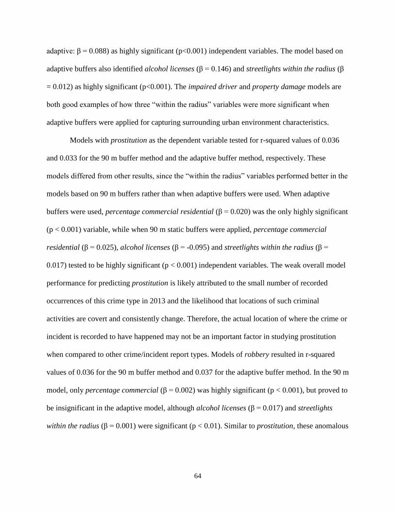
64
adaptive: β = 0.088) as highly significant (p<0.001) independent variables. The model based on
adaptive buffers also identified alcohol licenses (β = 0.146) and streetlights within the radius (β
= 0.012) as highly significant (p<0.001). The impaired driver and property damage models are
both good examples of how three “within the radius” variables were more significant when
adaptive buffers were applied for capturing surrounding urban environment characteristics.
Models with prostitution as the dependent variable tested for r-squared values of 0.036
and 0.033 for the 90 m buffer method and the adaptive buffer method, respectively. These
models differed from other results, since the “within the radius” variables performed better in the
models based on 90 m buffers rather than when adaptive buffers were used. When adaptive
buffers were used, percentage commercial residential (β = 0.020) was the only highly significant
(p < 0.001) variable, while when 90 m static buffers were applied, percentage commercial
residential (β = 0.025), alcohol licenses (β = -0.095) and streetlights within the radius (β =
0.017) tested to be highly significant (p < 0.001) independent variables. The weak overall model
performance for predicting prostitution is likely attributed to the small number of recorded
occurrences of this crime type in 2013 and the likelihood that locations of such criminal
activities are covert and consistently change. Therefore, the actual location of where the crime or
incident is recorded to have happened may not be an important factor in studying prostitution
when compared to other crime/incident report types. Models of robbery resulted in r-squared
values of 0.036 for the 90 m buffer method and 0.037 for the adaptive buffer method. In the 90 m
model, only percentage commercial (β = 0.002) was highly significant (p < 0.001), but proved to
be insignificant in the adaptive model, although alcohol licenses (β = 0.017) and streetlights
within the radius (β = 0.001) were significant (p < 0.01). Similar to prostitution, these anomalous

65
observations are likely due to the relatively low number of recorded occurrences of this crime
type (110 records in 2013).
Sex offence/indecent act resulted in weak OLS models with r-squared values of 0.021 and
0.039 for the 90 m and adaptive buffer methods, respectively. GRT bus stops within the radius
(90 m: β = 0.025, adaptive: β = 0.024) was the only independent variable that was highly
significant in both models. Percentage institution (β = 0.004) was highly significant (p < 0.001)
when 90 m buffers were applied and streetlights within the radius (β = 0.005) was highly
significant (p < 0.001) when adaptive buffers were used. This result is expected, since a diversity
of crimes and behaviours may be classified in the sex offence/indecent act category, and thus it
was not expected that this dependent variable would follow a distinct spatial pattern. Suspicious
person or vehicle had r-squared values of 0.055 and 0.088 with the 90 m and adaptive buffer
methods, respectively. While percentage institutional (β = 0.007) and GRT bus stops within the
radius (β = 0.097) tested to be highly significant variables (p < 0.001) when 90 m buffers were
used, alcohol licenses (β = 0.133), GRT bus stops (β = 0.097), and streetlights within the radius
(β = 0.012) were highly significant (p < 0.001) when adaptive buffers were applied. Regression
models of theft motor vehicle were very weak with r-squared values of 0.018 and 0.022 for the
90 m and adaptive buffer methods, respectively. The model based on 90 m static buffers resulted
in only percentage commercial (β = 0.006) and percentage industrial (β = 0.006) as significant
variables (p < 0.05). The adaptive buffer model results showed streetlights within the radius (β =
0.009) and percentage industrial (β = 0.009) as significant variables (p < 0.05). The overall
weakness of theft motor vehicle OLS models might be attributed to car thieves not wanting to
appear to be predictable to police and therefore, spatial patterns of such criminal activities may
appear randomly distributed throughout the study area.

66
Models of theft under $5,000 resulted in r-squared values of 0.089 with 90 m static
buffers and 0.094 with adaptive buffers. While only the adaptive buffer model identified alcohol
licenses (β = 0.851) and bus stops within the radius (β = 0.440) as highly significant (p < 0.001),
both models tested percentage commercial (90 m: β = 0.083, adaptive: β = 0.056) as a highly
significant variable (p < 0.001). This is notable, since this was one of only two dependent
variables for which percentage commercial tested to be significant using the adaptive buffer
method. This result is expected, since businesses such as retail stores can be desirable targets for
thieves, and would be more likely to report theft as it impacts their livelihood. Conversely, a
resident might be less likely to report theft of personal property given the time it takes to make a
report, and the low probability that it would result in their property being recovered.
7.2.2 OLS Buffer Results – Independent Variable Results
The full results of OLS Buffer regression models can be found in Table A1 (90 m) and
A2 (adaptive) in the Appendix section. Percentage residential proved to be one of the weakest
independent variables in the tested models. In the 90 m static buffer method, the variable was
only considered significant (p < 0.05) in three models (domestic dispute, as was expected,
dispute, and motor vehicle collision). It was not significant when the adaptive buffer method was
considered. It was originally hypothesised that this variable would be typically negatively related
to crime/reported incidents, since it is generally expected that most crime would happen in the
city centre away from the residential heavy suburbs. This appeared to be confirmed by initial
maps created with the data, such as Figure 23, which shows lower levels of residential buildings
occurring in downtown areas. However, in the three models where percentage residential was a
significant variable, it was a negative coefficient only once. Percentage recreation also proved to
be a weak variable in the estimated models. Like residential buildings, recreational buildings

67
were generally hypothesised to negatively affect crime report levels. Unlike residential buildings,
however, in both the 90 m and adaptive buffer methods, thirteen of the eighteen estimated
models were negative.
Percentage institutional proved to be significant in most of the estimated models. It
tested to be significant (p < 0.05) in most of the 90 m buffer models and in half of the adaptive
buffer models. The coefficient was almost always positive. The fact that percentage institutional
was typically a significant and positive variable may not be due to the institutional buildings
themselves, but rather because of the large concentration of such buildings within the downtown
core and thus matching the spatial pattern of much of the crime/incident report variables.
Percentage commercial performed better in the 90 m method than the adaptive method, as it was
significant (p < 0.05) in most 90 m models but only in two of the adaptive models. It also tested
to be a positive coefficient in all models.
Percentage industrial was rarely a significant variable, although it was significant in both
theft motor vehicle models and was significant in the break and enter and dispute models based
on 90 m static buffers (p < 0.05). It is possible that crime is an atypical occurrence in industrial
park areas. It mostly tested to be a positive variable in the OLS models (fifteen of eighteen
models) based on 90 m buffers, but it tended to be a negative variable when adaptive buffers
were used (ten of eighteen models). Percentage utility was also rarely significant (p < 0.05) and
negative in all but four of the 36 models. Percentage agricultural was also an insignificant
independent variable with crime/reported incidents and mainly negatively related when 90 m
buffers were considered, but tested to be generally positive when adaptive buffers were applied.
Percentage utility and percentage agricultural are both likely insignificant factors due to the
very few occurrences of these land uses within Kitchener.

68
Percentage commercial residential was significant (p < 0.05) in six of the eighteen
models using the 90 m buffer method and in eight of the eighteen models using the adaptive
buffer method. The full statistical are shown in Tables A1 (90 m) and A2 (adaptive) of Appendix
sections. It was mostly a positive relationship, but tested to be negative and significant (p < 0.01)
in the models of impaired driver (β = -0.003) using the 90 m buffer method and motor vehicle
collision (β = -0.083) based on the adaptive buffer method. Similar to percentage institutional, it
is possible that this variable was generally significantly related to crime/reported incidents, since
buildings of both commercial and residential land uses tend to be located in the downtown area.
Since the downtown area is more heavily developed, it is more common to find residential space
and businesses in the same buildings, which result in more multi-use and access by people
throughout different times of the day.
Percentage greenspace was only significant (p < 0.05) in one model of motor vehicle
collision based on 90 m buffers (β = -0.018). Although the independent variable tested to be
mostly positive when the 90 m buffer method was used, it was a mostly negative coefficient
when the adaptive buffer method was applied. It would seem that in Kitchener, parks do not
function as crime attractors or criminal marketplaces that some studies, such as DeMotto and
Davies (2006), have suggested them to be.
The alcohol licenses within the radius was one of the best fitting independent variables,
especially when adaptive buffers were applied. The variable was significant in most models
based on 90 m buffers and was highly significant (p < 0.001) in almost all models where
adaptive buffers were used. It tested to be a positive coefficient for most OLS models. Alcohol
licenses was originally expected to be a well-fitting variable, since previous studies have linked
alcohol sales to increases in crime (Day et al., 2012; Kumar & Walyor, 2003).

69
GRT bus stops within the radius tested to be the most significant independent variable of
crime/reported incidents when both buffer methods were applied. It was significant (p < 0.05) in
fourteen of the 90 m buffer models and sixteen of the adaptive buffer models. It was also highly
significant (p < 0.001) in eleven of the 90 m buffer models and thirteen of the adaptive buffer
models. It was positive in all but one model in both methods. Bus stops within the radius was
expected to be a crime attractor, since these are locations where people tend to congregate
outdoors, which may create opportunities for criminals.
Streetlights within the radius was also a significant predictor of crime/reported incidents.
It was significant (p < 0.05) in half of the 90 m models and in all but two of the adaptive models.
It was a positive coefficient in all but three models, all of which were 90 m models where it was
not a significant variable. These findings are interesting when considering the original
expectation that streetlights would help reduce crime, since increase lighting may potentially
deter criminal activity. It is possible that streetlights actually attract crime, because they can
make potential criminal targets more visible and highlight opportunities for criminal activity.
7.2.3 OLS Buffer Results – Summary of Key Findings
Overall the models estimated with the OLS Buffer methodology (both 90 m and
adaptive) were quite weak with the largest r-squared value as 0.227. This suggests that a weak
relationship between crime and the urban environment exists in the Waterloo Region. This result
may be due to missing predictor variables, such as socio-economic variables, which may affect
the probability of a crime incident occurring.
Of the eighteen crime/reported incident types used in the OLS buffer methodology, many
were associated with the largest r-squared values were linked to alcohol consumption, either
directly (such as intoxicated person, which resulted in the strongest model in both the 90 m and

70
adaptive models), or indirectly (such as in the case of disturbance and assault). This suggests
that alcohol licenses was a strong predictor in crime/reported incidents since this independent
variable was highly significant within these models. The strength of alcohol licenses as a
predictor is further evidenced by its large coefficient values particularly within these stronger
models whose dependent variable is directly or indirectly linked to alcohol. Bus stops tested to be
consistently significant based on OLS buffer methodology. According to Routine Activity
Theory, it is theorized that this is due to bus stops being places were people congregate outdoors
and thus creating opportunities for criminals (Cohen & Felson, 1979). Streetlights also
consistently tested to be a significant variable, but more so with adaptive models than the 90 m
buffer models. Although streetlights was hypothesised to have a negative relationship with
crime/reported incidents, its relationship was positive in all models where streetlights tested to be
significant. It is believed that the relationship was positive due to individuals wanting to stay
within lit areas at night, creating criminal opportunities for offenders. Overall, alcohol licenses,
bus stops, and streetlights were strong predictors of crime/reported incidents, which may
potentially be attributed to the fact that they are also indicators of presence of human activity,
especially in the case of bus stops and streetlights.
Percentage institutional, commercial, and commercial residential were the building
footprint variables that most frequently tested to be significant, though percentage commercial
was far less frequently significant when the adaptive buffer was used. It is likely that the
frequently significant relationship between percentage commercial residential and institutional
and crime/reported incidents is attributed to their concentrated spatial distribution in downtown
areas, rather than actual strong relationships between reported crime incidents and these
predictor variables.

71
7.3 OLS Adaptive Kernel Density Estimation (AKDE) Results
Overall, the OLS models based on AKDE data input tested to be weaker than the OLS
models using both static and adaptive buffers. Only three models, those with the dependent
variables disturbance, intoxicated person, and unwanted person, resulted in r-squared values
above 0.1. It is possible that these crime/reported incidents performed better, since these crime
types are more likely to be committed by people who are travelling on foot, playing to the
strength of the AKDE models of detecting the spatial influence around a facility. However, since
these dependent variables were among the strongest in the buffer method, it is more likely that
this is a result of similar dependent variables performing comparably with the same independent
variables. All AKDE models were highly significant with the exception of the homicide model.
The full results of the OLS AKDE models are shown in Table A5 in the Appendix.
7.3.1 OLS AKDE Results – Model Results
As previously discussed, the AKDE models (when using OLS regression) with the three
strongest r-squared values were those with the dependent variables disturbance, intoxicated
person, and unwanted person. Disturbance was the strongest of these models with an r-squared
value of 0.128. The AKDE value of licensed restaurants (β = 0.030), secondary schools (β =
0.206), and universities (β = 0.282) were all highly significant (p < 0.001) in this model. This is
particularly interesting since the AKDE values for universities were only highly significant (p <
0.001) in two of the eighteen AKDE OLS regression models. This is consistent with
expectations, since alcohol provided by licensed restaurants could result in intoxicated people,
who may cause disturbances. Also, the students of high schools and post-secondary institutions
are often associated with age groups that are typically associated with causing disturbances.
Similar to both the 90 m and adaptive buffer models, intoxicated person resulted in one of the

72
strongest tested models with an r-squared value of 0.123 when the AKDE method was applied.
This perhaps shows that the dependent variable has a strong spatial relationship with its
surrounding urban environment. The AKDE value for GRT bus stops (β = 0.009), licensed
restaurants (β = 0.027), and universities (β = 0.286) were highly significant (p < 0.001) variables
in this model. Similar to the disturbance model, it is believed that licensed restaurants played a
key role, since such restaurant establishments provide alcohol, which may in turn increase
chances of intoxication and associated behaviours. Similar to the disturbance model, it is
believed that universities were a significant independent variable in this model, since students of
post-secondary education institutions are perceived to drink more heavily. On the other hand,
unlike the model of disturbance, secondary school AKDE values were not significant in the
intoxicated person model, likely due to the minimum drinking age preventing high school
students to drink excessively or having access to alcohol. This perhaps indicates that drinking
age laws are an effective deterrent or at least deters these students from drinking near their high
school. The OLS model of unwanted person had an r-squared value of 0.113. GRT bus stops (β =
0.023), licensed restaurants (β = 0.057), and places of worship (β = 0.073) were all highly
significant (p < 0.001) independent variables based on AKDE models. The variable places of
worship unexpectedly resulted in a positive coefficient.
The assault model had an r-squared value of 0.084. The AKDE values for GRT bus stops
(β = 0.005), licensed restaurants (β = 0.012), secondary schools (β = 0.098) and WRPS police
stations (β = 0.281) were all highly significant (p < 0.001) in this model. The result of licensed
restaurants as a significant predictor of assault was expected. However, the police stations
variable was quite unexpected, especially considering that it was a positive variable. The OLS
model of drugs had an r-squared value of 0.068, identifying the same highly significant (p <

73
0.001) variables as the assault model. In this case, it is believed that some of these variables,
such as police stations (β = 0.366) and licensed restaurants (β = 0.007) were more likely
indicators of the downtown area, where drugs might be sold. Motor vehicle collision had an r-
squared value of 0.058. Similar to the OLS model of motor vehicle collision based on static and
adaptive buffers, it was not expected that this dependent variable would have a strong model,
since it is not considered to be an intentional crime. GRT bus stops (β = 0.052) and LCBO and
Beer Store locations (β = 0.797) were the only two highly significant (p < 0.001) variables in this
model. These independent variables are likely indicators of vehicle mobility. Similarly, LCBO
and Beer Store locations are generally built at locations that are convenient for drivers to access.
The model of property damage as the dependent variable had an r-squared value of 0.057.
Licensed restaurants (β = 0.010) and WRPS police stations (β = 1.217) were the only two highly
significant (p < 0.001) independent variables.
The domestic dispute model had an r-squared value of 0.034. The AKDE value for GRT
bus stops (β = 0.022) was the only highly significant (p < 0.001) variable in this model, possibly
due to the more widely distributed and residential nature of this crime/reported incident type,
which matches the distribution of bus routes and stops. Impaired driver and suspicious person or
vehicle both resulted in an r-squared value of 0.030. Whereas GRT bus stops (β = 0.010) was the
only highly significant (p < 0.001) independent variable in the models of suspicious person or
vehicle, while LCBO and Beer Stores (β = 0.048), licensed restaurants (β = 0.003) and
universities (β = -0.049) were significant (p < 0.01) in the model of impaired driver. It is
interesting to note that licensed restaurants was not significant in the 90 m buffer OLS model for
impaired driver (though it was significant in the adaptive buffer OLS model). This perhaps
reflects the AKDE raster’s ability to show the slowly dissipating influence of the licensed

74
restaurants. While the 90 m and adaptive buffer methods only detect the environment features
within an area approximately between each intersection and its neighbouring intersections, the
AKDE method is able to detect the influence of environment features between 300 and 600 m
away, depending on the assigned bandwidth. As impaired drivers will typically drive more than a
block away from the licensed restaurant where they became impaired before being caught, only
the AKDE method would be able to detect the influence of the restaurant at the intersection
where the arrest was made. The model of theft under $5,000 had an r-squared value of 0.028.
The AKDE value for GRT bus stops (β = 0.050) and LCBO and Beer Store locations (β = 0.829)
were both highly significant (p < 0.001). The significance of GRT bus stops on theft makes
sense, since thieves may target transit areas and encounter more opportunities to steal items left
unattended by bus passengers. Universities were expected to be significant for similar reasons as
bus stops, since students leaving electronics and other valuables unattended may increase the
potential for theft. It is common to see police bulletins warning students to guard their valuables
while on campus. However, this was not tested to be a significant variable in this model
estimation. The dispute model weak with an r-squared value of 0.025. GRT bus stops (β = 0.012)
was the only highly significant (p < 0.001) independent variable in this model.
The robbery model had an r-squared value of 0.023. This low r-squared value is likely
partially due to this crime/reported incident type’s rare occurrence. GRT bus stops (β = 0.001)
and secondary school (β = 0.026) tested to be highly significant (β = 0.001) independent
variables. As previously mentioned, bus stops represent locations where opportunities may exist
for robbery, especially where people may wait alone or in small numbers outdoors at various
times of day and night. Models of prostitution and theft motor vehicle had r-squared values of
0.022. Only places of worship (β = 0.020) was tested as a significant (p < 0.001) predictor of

75
prostitution, while WRPS police stations (β = 0.358) was a significant (p < 0.001) predictor of
theft of motor vehicle. Such significant relationships were puzzlingly and unexpected, which may
be more of an artifact of how the data was collected and recorded, or confounded by other factors
not considered in the model.
Sex offence/indecent act resulted in one of the weakest OLS models with an r-squared
value of 0.015. The AKDE values of secondary school and GRT bus stops were highly
significant independent variables. As noted in the previous regression analyses with buffer
methods, the low r-squared value reflects the lack of spatial patterns for such crime/reported
incident types. The model of break and enter also resulted in a weak r-squared value of 0.014.
Only GRT bus stops was highly significant within the model. This may reflect the similar spatial
distribution of this built environment feature with the spatial patterns of this type of
crime/reported incident, especially in residential areas. Homicide showed the lowest r-squared
value, likely due to the rare number of cases recorded in the WRPS dataset, making this type of
crime/report incident difficult to model. Similar to the prostitution model, the only significant
independent variable for modelling homicide was places of worship, which was again
unexpectedly a positive relationship.
7.3.2 OLS AKDE Results – Independent Variables Results
Characteristics of the built and natural environment as independent variables tested to
have varying degrees of significance within the AKDE models. Although most variable
coefficients were positive, several variables were negatively related and significant within a
small number of tested OLS regression models. Similar to previous sections, the full statistical
results of the AKDE OLS regression models are shown in Table A5.

76
Elementary schools proved to be a weak predictor of crime/reported incidents. It tested to
have a significant (p < 0.05), negative relationship with motor vehicle collision (β = -0.124),
suggesting that fewer collisions occur close to schools. Although a negative relationship between
schools and crime/reported incidents was expected in this study, since committing crimes near
schools are often considered to be taboo, the variable was only negative in half of the tested
models. This is perhaps associated with the relatively even distribution of elementary schools
throughout Kitchener-Waterloo with pre-planned locations.
GRT bus stops tended to be highly significant (p < 0.001) and positively related with
crime/reported incidents in most tested models. This is consistent with previous results from the
OLS models based on buffer analysis, which suggests that bus stops represent locations where
people wait alone or in small numbers outdoors, thus creating opportunities for someone to
commit a crime. However, bus stops may also simply be an indicator of human activity.
LCBO and Beer Store locations were significantly (p < 0.05) related to crime/reported
incidents in five tested regression models. Interestingly, this variable’s values were not
significant in the model of intoxicated person, which was expected to have a strong relationship.
This is despite the fact that licensed restaurants values were highly significant in the model of
intoxicated person. This is perhaps due to the fact that people who purchase alcohol from a store
will likely take it elsewhere before they consume it, making it more difficult to estimate the
spatial effect that stores may have on intoxication. Conversely, when people purchase alcohol at
a restaurant or bar, they would likely consume it on-site and observable effects of intoxication
would likely occur on the premises. This enables spatial effects of licensed restaurants on
crime/reported incidents to be more easily identified and modelled.

77
The AKDE values for libraries, community centres and arenas was only significant (p <
0.05) in three models and positively related to most crime/reported incidents. This was not
expected to be a significant predictor variable as it had moderately few locations recorded in the
dataset.
Licensed restaurants was the second best fitting variable and was expected to perform
well. It tested to be a significant (p < 0.05) predictor in most models, including crime/reported
incidents related to alcohol, such as intoxicated person and impaired driver, as well as
disturbance and assault, which could be associated with alcohol consumption.
Places of worship performed oddly well in tested models, being significant (p < 0.05) in
five and highly significant (p < 0.001) in three. It was also unexpectedly positive in all but four
models. These anomalies might be due to the fact that many older churches are located in the
downtown area. It should be noted that places of worship was typically significant in models
with very low r-squared values and thus, not deemed to be a significant predictor of
crime/reported incidents.
Secondary schools proved to be a well-fitting independent variables. It was significant (p
< 0.05) in half of the models, highly significant (p < 0.001) in five of the models, and positive in
all but two of the models. Some relationships were expected, such as with disturbance, while
others, such as robbery, unexpectedly performed well with secondary schools.
Hospitals, of which there were only three in the region, was the weakest of all the
independent variables. It was not significant in any of the tested models. Similar to the libraries,
community centres and arenas variable, this variable was included to add to the overall
completeness of the tested set of variables, and it was not expected to be a good predictor of
crime/reported incident locations.

78
Universities performed better than expected given the low number of such features in the
dataset, being significant (p < 0.05) in six models and highly significant (p < 0.001) in two. As
expected, it performed well with alcohol-related models, but as previously mentioned, it
performed unexpectedly poorly in theft under $5,000 as it was believed that theft, particularly of
personal electronics and bicycles, was common on university campuses. It was also negative and
significant in the models for impaired driving and robbery. This would make sense in the former
case, since universities are well connected to public transportation and university students are
less likely to own a motor vehicle and may be more conscious about the dangers of drunk
driving. It is interesting to note that only two models resulted in the university variable being
identified as highly significant and also resulted in the largest r-squared values tested among the
OLS AKDE models.
WRPS police stations also performed surprisingly well in the tested models. It was
significant (p < 0.05) in eight of the models and highly significant (p < 0.001) in four.
Unexpectedly, it was positive in almost all models. This might be due to the fact that police
stations are located in areas of high human activity where crimes are more frequently committed,
because they are evenly distributed across the region, or because crimes are easier to report and
are more easier to respond to if they are near a police station. This could also be due to elevated
monitoring around police stations as they are the locations where police officers are based,
ensuring more crime will be addressed and recorded in these areas.
7.3.3 OLS AKDE Results – Summary of Key Findings
The OLS AKDE regression models yielded weaker results than the OLS buffer
methodology (both 90 m and adaptive buffer approaches) as evidenced by weaker r-squared
values. The weak relationship observed between crime and urban environment characteristics

79
may be attributed to missing socio-economic variables or other factors that may be important to
predicting the location of crime incidents, as well as other missing built or natural environmental
characteristics that were not considered in estimated AKDE regression models.
The crime/reported incident types that were most strongly associated with urban
environmental characteristics tended to be based on OLS buffer methodology. Licensed
restaurants was a highly significant variable, although liquor stores alone were rarely significant.
Bus stops were again identified as a significant variable. This is likely due to the nature of people
gathering in or transiting through such spaces and thus creating opportunities for criminals, as
well as being an indicator of human activity.
Secondary schools, universities and police stations also proved to be significant, although
in fewer of the regression models. Universities was highly significant amongst all tested models.
Police stations resulted in an unexpectedly positive relationship with crime/reported incidents,
although this is likely due to the downtown location of most police stations. Overall, the
statistically significant relationships of hospitals, universities, and police stations with crime
incidents were questionable given the fact that there were a limited number of samples of each
type of built environment feature.
7.4 Logistic Buffer Regression Results
Theoretically, it is difficult to compare the strength of logistic regression models to each
other and to the strength of OLS regression models. Nevertheless, the results from OLS
regression and logistic regression results based on static and adaptive buffer analysis exhibited
some similarities. For example, all OLS and logistic regression models except for models of
homicide resulted in overall p-values that were highly significant (p < 0.001). When the logistic

80
regression models had a relatively high chi-squared value, the corresponding OLS regression
model typically had a relatively large r-squared value. In both the 90 m and adaptive buffer
methods, when the logistic regression models resulted in a low chi-squared value, the
corresponding OLS regression model typically had a small r-squared value. The logistic
regression models did, however, differ from the OLS regression models in many ways. In some
cases, this might suggest that different relationships exist between the individual crime/reported
incident types and environment features. The significance levels that were achieved by the
independent variables in both types of regression models would often vary, particularly in the
case of variables spatially concentrated in downtown areas. It was also noted that the models
with the largest numbers of significant variables were often those whose dependent variables
were present at the most intersections. The following sections will explore these differences. The
full statistical results are shown in Table A3 for the 90 m buffer logistic regression models and
Table A4 for the adaptive buffer logistic regression models, both in the Appendix section.
7.4.1 Logistic Buffer-based Regression – Model Results
The 90 metre buffer logistic regression model that used the dependent variable assault
was similar to the 90 metre OLS assault model that used the same dependent variable. GRT bus
stops (β = 0.151 in logistic regression) were highly significant (p < 0.001) in both models. The
adaptive logistic regression model for assault followed a similar pattern. GRT bus stops (β =
0.211 in logistic regression) and streetlights within the radius (β = 0.032 in logistic regression)
again were both highly significant (p < 0.001) in the logistic and OLS regression models.
With break and enter as the dependent variable, the model based on 90 m buffers tested
in percentage institutional (β = 0.020 in logistic regression) and industrial (β = 0.018 in logistic
regression) at the same level of significance (p < 0.01) for both the logistic and OLS regression

81
approaches, whereas bus stops (β = 0.096 in logistic regression) was less significant (p < 0.05)
and alcohol licenses (β = 0.197 in logistic regression) was more significant (p < 0.01) in logistic
regression. For the adaptive models, however, only bus stops (β = 0.211 in logistic regression)
maintained the same significance level (p < 0.001) between OLS and logistic regression, while
percentage institutional (β = 0.024) and industrial (β = 0.021), alcohol licenses (β = 0.164), and
streetlights (β = 0.032) tested to be significant (p < 0.05) in the logistic regression model.
In the regression models estimated for dispute cases, more significant independent
variables were identified in the OLS regression models, particularly in the case of the models
based on 90 m static buffers. Although bus stops was the only significant variable in the logistic
regression model based on 90 m buffers (β = 0.183, p < 0.001), percentage residential,
commercial, and industrial were also significant in the OLS model. The adaptive OLS model,
however, identified only slightly more significant independent variables than the adaptive
logistic regression model as bus stops (β = 0.220 in logistic regression) and streetlights (β =
0.036 in logistic regression) were highly significant (p < 0.001) in both models, but alcohol
licenses was only significant in the OLS model. This advantage might be due to deviant
individuals getting into multiple disputes over time in the same general area, which would be
more amenable to being estimated by the OLS regression model, which takes into account
multiple events at the same intersection. Disturbance followed a similar pattern to the dispute
models, since the OLS models’ independent variables were more significant than in the logistic
regression models, again especially in the case of the 90 m models. In the 90 m buffer models,
while only bus stops (β = 0.220 in logistic regression) and streetlights (β = 0.220 in logistic
regression) were significant (p < 0.01) in both the OLS and logistic regression models, alcohol
licenses and percentage institutional, utility, and commercial residential were also significant in
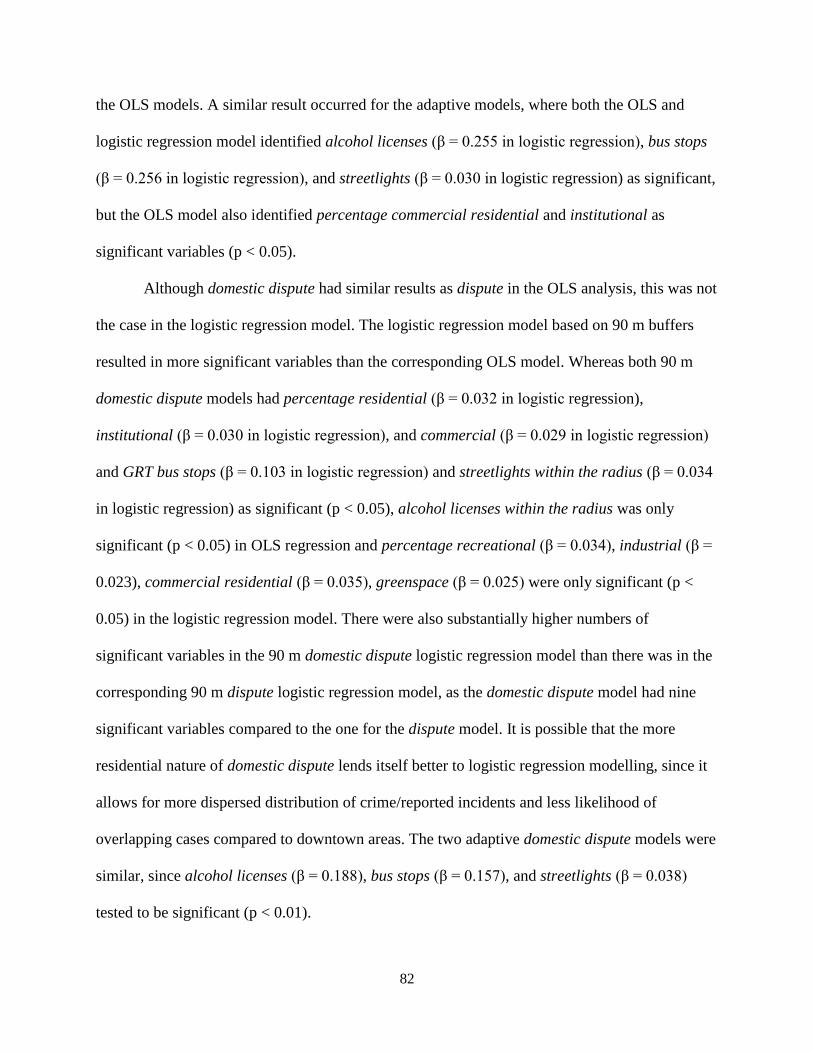
82
the OLS models. A similar result occurred for the adaptive models, where both the OLS and
logistic regression model identified alcohol licenses (β = 0.255 in logistic regression), bus stops
(β = 0.256 in logistic regression), and streetlights (β = 0.030 in logistic regression) as significant,
but the OLS model also identified percentage commercial residential and institutional as
significant variables (p < 0.05).
Although domestic dispute had similar results as dispute in the OLS analysis, this was not
the case in the logistic regression model. The logistic regression model based on 90 m buffers
resulted in more significant variables than the corresponding OLS model. Whereas both 90 m
domestic dispute models had percentage residential (β = 0.032 in logistic regression),
institutional (β = 0.030 in logistic regression), and commercial (β = 0.029 in logistic regression)
and GRT bus stops (β = 0.103 in logistic regression) and streetlights within the radius (β = 0.034
in logistic regression) as significant (p < 0.05), alcohol licenses within the radius was only
significant (p < 0.05) in OLS regression and percentage recreational (β = 0.034), industrial (β =
0.023), commercial residential (β = 0.035), greenspace (β = 0.025) were only significant (p <
0.05) in the logistic regression model. There were also substantially higher numbers of
significant variables in the 90 m domestic dispute logistic regression model than there was in the
corresponding 90 m dispute logistic regression model, as the domestic dispute model had nine
significant variables compared to the one for the dispute model. It is possible that the more
residential nature of domestic dispute lends itself better to logistic regression modelling, since it
allows for more dispersed distribution of crime/reported incidents and less likelihood of
overlapping cases compared to downtown areas. The two adaptive domestic dispute models were
similar, since alcohol licenses (β = 0.188), bus stops (β = 0.157), and streetlights (β = 0.038)
tested to be significant (p < 0.01).

83
The OLS model based on 90 m static buffers for drugs identified more significant
independent variables than the logistic regression model. This may be due to the fact that the
drugs variable has a large concentration of occurrences in downtown areas. These multiple
occurrences at the same street intersections are not present as binomial occurrences in the logistic
regression modelling technique. The adaptive model results were rather similar between OLS
and logistic regression, with logistic regression identifying one additional significant variable
(percentage commercial residential, β = 0.043, p < 0.01).
The homicide models in logistic regression had, similar to the OLS regression models, by
far the lowest overall significance values, and were the only models in the logistic regression not
considered to be significant. These models also resulted in the lowest chi-squared values (90 m:
χ2 = 13.495, adaptive: χ2 = 6.944. No logistic regression models of homicide identified
significant independent variables, while both OLS models identified percentage commercial
residential as significant.
With the impaired driver models, the performance of the independent variables was quite
different in the 90 m buffer-based logistic regression model compared to the corresponding OLS
model. Although bus stops (β = 0.178 in logistic regression) were significant (p < 0.01) in both
models, only the OLS model identified percentage commercial residential as highly significant
(p < 0.001), and only the logistic regression model identified percentage residential (β = -0.017)
and streetlights (β = 0.042) as significant (p < 0.01). The impaired driver’s adaptive buffer
logistic regression models were more similar to the corresponding OLS models than the 90 m
static buffer method. Both models identified bus stops (β = 0.180 in logistic regression) and
streetlights (β = 0.035 in logistic regression) as highly significant (p < 0.001). However, in OLS

84
regression, the alcohol licenses variable was highly significant (p < 0.001), and in the logistic
regression model, percentage residential (β = -0.019) was moderately significant (p < 0.05).
With intoxicated person, both 90 m static buffer models identified bus stops (β = 0.313 in
logistic regression) and streetlights (β = 0.069) as significant (p < 0.01), but only the OLS model
identified alcohol licenses as highly significant (p < 0.001). Although the logistic regression
models tend to be less influenced by the independent variables concentrated in the downtown
area, the lack of significance in logistic regression of alcohol licenses, a variable so directly
linked to the dependent variable, suggests weakness in the 90 m logistic models. Conversely, the
adaptive logistic regression model identified alcohol licenses (β = 0.344 in logistic regression) as
highly significant (p < 0.001), as was the case in the corresponding OLS model. Both adaptive
models also identified bus stops (β = 0.292 in logistic regression) as highly significant (p <
0.001).
The motor vehicle collision logistic regression models had in the largest chi-square values
with both the 90 m buffer (χ2 = 347.16) and the adaptive buffer (χ2 = 421.15). The full statistical
results of the logistic regression buffer models are shown in Tables A3 (90 m) and A4 (adaptive)
in the Appendix. The performance of the significant variables in the 90 m models was quite
different to how they performed in the OLS models, perhaps suggesting different relationships
exist between this type of crime/reported incidents and the environment than was identified by
OLS regression. While both models identified percentage commercial (β = 0.012 in logistic
regression), bus stops (β = 0.346 in logistic regression) and streetlights (β = 0.055 in logistic
regression) as being significant (p < 0.01), only the OLS model identified percentage greenspace
and residential as significant, and only the logistic regression model tested percentage
institutional (β = 0.016) and industrial (β = 0.012) to be significant (p < 0.01). In the case of the

85
adaptive models, both identified percentage commercial residential (β = 0.032 in logistic
regression), alcohol licenses (β = 0.170 in logistic regression), bus stops (β = 0.275 in logistic
regression) and streetlights (β = 0.036 in logistic regression) as significant (p < 0.05), whereas
only the OLS model identified percentage commercial as significant (p < 0.001). Only the
logistic regression model tested percentage institutional (β = 0.018) and recreational (β = 0.031)
to be significant (p < 0.05). This difference could be accounted for by the fact that, as mentioned
before, motor vehicle collision is not necessarily an intentional crime, and therefore might
behave quite differently than other dependent variables in OLS regression versus logistic
regression.
The property damage models exemplified the difference between the OLS and logistic
regression results. In the 90m logistic regression model, five variables were significant (p <
0.01), whereas the corresponding OLS model identified three significant variables (p < 0.01).
This is an example of how logistic regression tended to be a better fitting model for dependent
variables that were less centrally concentrated, such as property damage. The adaptive models
were similar in results with the main difference being percentage institutional identified as being
highly significant (p < 0.001) in the OLS model, but not significant in the logistic regression
model.
Prostitution resulted in weaker logistic regression models than the OLS regression
models. While the 90 m buffer-based OLS model identified four significant variables (p < 0.05),
including three of which were highly significant (p < 0.001), the 90 m buffer-based logistic
regression identified only one significant (p < 0.01) variable, streetlights (β = 0.075). Fewer
differences were observed between the two adaptive buffer-based models: the OLS model
resulted in three significant variables (p < 0.05), whereas the logistic regression model identified

86
two significant variables (p < 0.05). Both OLS and logistic regression models of prostitution
were very weak. Likewise, the OLS and logistic regression models for robbery were weak in
terms of goodness of fit. The poor regression model results for lack of fit of prostitution and
robbery is likely due to the low number of street intersections included in the dataset at which
this crime/reported incident type occurred. In the case of robbery, it is likely that a criminal
would choose different locations to commit robbery so that his or her actions do not follow an
expected pattern, thus making their crimes more difficult to model or predict. The models of sex
offence/indecent act also had weak results with few significant variables identified in both OLS
and logistic regression models. The 90 metre buffer-based OLS model for sex offence/indecent
act resulted in three significant variables, while the logistic regression model identified only one
significant variable. Similar results were observed in both adaptive buffer-based regression
results. The models for sex offence/indecent act resulted in a weak logistic regression model.
Models of suspicious person or vehicles resulted in more significant variables identified
in logistic regression models than with OLS regression for the 90 m buffer method. Whereas the
percentage intuitional (β = 0.024 in logistic regression) and commercial (β = 0.014 in logistic
regression), bus stops (β = 0.113 in logistic regression) and streetlights (β = 0.024 in logistic
regression) were significant (p < 0.05) in both models, the logistic model also identified
percentage residential (β = 0.010), percentage industrial (β = 0.012), and percentage greenspace
(β = 0.010) as significant variables (p < 0.05). These results are likely due to the high presence
count and the widely distributed nature of this crime/reported incident type. Estimated regression
models based on the adaptive buffer method resulted in similar findings.
The logistic regression for theft motor vehicle was one of the weakest models tested,
similar to the OLS regression results. Percentage industrial (β = 0.020 in logistic regression) and

87
commercial (β = 0.016 in logistic regression) were significant variables (p < 0.05) in both 90 m
OLS and logistic regression and bus stops (β = 0.116) were also significant (p < 0.01) in the
logistic regression model. However, regression models differed when the adaptive buffer method
was applied. The corresponding OLS model identified two significant variables, namely
streetlights and percentage industrial (p < 0.05). The logistic regression tested to be a stronger
model with bus stops, streetlights, and alcohol licenses being significant (p < 0.01). It is unclear
why such differences exist, however, it is notable that theft motor vehicle is one of the few cases
where the adaptive buffer-based logistic model was better fitting than the corresponding OLS
regression model. It is interesting to note that percentage industrial, an urban environmental
characteristic that rarely tested to be significant, was generally associated with cases of theft
motor vehicle, as was the case in the OLS models, suggesting a relationship between the two
variables.
Theft under $5,000 estimated models were quite different between OLS and logistic
regression methods when using 90 metre static buffer input data. In the OLS model, percentage
commercial and institutional were significant (p < 0.05) variables. The logistic regression model
yielded a better goodness of fit with more significant (p < 0.01) variables, including percentage
residential (β = 0.025), percentage recreational (β = 0.041), percentage institutional (β = 0.034),
percentage commercial (β = 0.029), percentage industrial (β = 0.029), percentage greenspace (β
= 0.021), bus stops (β = 0.099), and streetlights (β = 0.028). The fact that many variables tested
to be significant in the logistic regression analysis is likely due to the fact that theft under $5,000
likely occurs in more locations dispersed within the city. Results of the adaptive buffer-based
regression models were similar. While both regression models identified alcohol licenses (β =
0.202 in logistic regression), bus stops (β = 0.126 in logistic regression), and streetlights (β =

88
0.042 in logistic regression) as significant (p < 0.05) variables, the OLS regression model also
identified percentage commercial as highly significant (p < 0.001).
Finally, unwanted person was modelled based on both 90 m and adaptive buffer methods
of data input. Notably, many variables tested to be significant in both of the 90 m buffer-based
models (i.e., percentage institutional, percentage commercial, percentage commercial
residential, bus stops, and streetlights), although to differing levels of significance. Also,
percentage utility and alcohol licenses were only significant within the OLS regression model
and percentage industrial (β = 0.016) was only significant (p < 0.01) in the logistic regression
model. In the case of the adaptive buffers, both OLS and logistic regression models identified
alcohol licenses (β = 0.294 in logistic regression) and bus stops (β = 0.194 in logistic regression)
as significant (p < 0.01) variables, but only the OLS regression model identified percentage
institutional and percentage commercial residential as significant (p < 0.01), while streetlights
(β = 0.029) was only significant (p < 0.001) in logistic regression.
In general, the 90 m static buffer OLS models identified more variables as significant and
at higher levels of significance than their corresponding logistic regression models. The
exception were namely crime/reported incident types that were more geographically dispersed or
less concentrated in the downtown area. The adaptive buffer-based models, however, exhibited
few differences between logistic and OLS regression models, with only a few exceptions.
7.4.2 Logistic Buffer-based Regression – Independent Variable Results
In general, percentage residential tested to be more significant when logistic regression
models were applied, rather than OLS regression models. When 90 m static buffer data were
used, percentage residential was significant (p < 0.05) in only three of the OLS models, whereas
it was significant (p < 0.05) in five of the logistic regression models. Furthermore, in the 90 m

89
buffer-based models, percentage residential was highly significant (p < 0.001) in two of the
logistic regression models (impaired driver and theft under $5,000), but was not highly
significant in any OLS models. Notably, this relationship was negative and highly significant (p
< 0.001) in the 90 m buffer logistic regression model of impaired driver cases, but was positive
in all other 90 m buffer logistic regression models that were tested. This is perhaps due to the
lack of multiple occurrences of impaired driver at downtown intersections where RIDE
programs may be set up, resulting in areas outside the downtown core with more residential
buildings, which tested to be more significant.
Regression results for percentage recreation did not differ significantly between logistic
regression and OLS regression specifications, and resulted in poor overall results. In the 90 m
buffer models, the variable was significant (p < 0.05) twice in the logistic regression models and
once in the OLS models and in the adaptive models, it was significant (p < 0.05) once in the
logistic regression models and never in the OLS models. Interestingly, the variable was highly
significant (p < 0.001) in the theft under $5,000 logistic regression model with 90 m buffer data.
Percentage recreation was found to be mostly positively related to crime/reported incidents in
logistic regression models.
Percentage institutional was also quite similar between the logistic regression and OLS
regression results based on the 90 m buffer method, but not in the adaptive buffer models. In the
adaptive models, percentage institutional was significant (p < 0.05) in eight as opposed to five
models between the OLS and logistic regression results, respectively. It was also highly
significant (p < 0.001) in three of the eight adaptive buffer-based OLS models where it was
significant (p < 0.05), but not in the logistic regression models. Such differences may be due to
the OLS models allowing for multiple crime/reported incidents to be counted at street

90
intersections. Since most crime/reported incident types and percentage institutional are spatially
concentrated downtown, it allows for a spatial relationship to be more easily identified between
crime/reported incidents and this building type in an OLS regression model specification.
Percentage commercial was more significant within the OLS regression models. This
was particularly the case when 90 m buffer data were used. Differences were less pronounced in
the adaptive buffer models, where percentage commercial was only significant in two the OLS
models (highly significant (p < 0.001) both times), and it was not significant in the logistic
regression models. This may again be due to the fact that independent variables typically
representative of downtown areas, such as percentage commercial, tested to be more significant
in OLS regression models with crime/reported incident types that are more concentrated in the
downtown area.
Percentage industrial was a more significant variable in logistic regression than in OLS
regression based on 90 m buffers. It was significant (p < 0.05) in eight of the logistic regression
models tested, but only three of the OLS models. Similar to percentage residential, a possible
explanation for this is that logistic regression only examines presence/absence of the dependent
variable. Industrial parks, where this building type is most common and which are located further
away from the downtown core in Kitchener, may perform better in logistic regression models,
since this regression method does not take into account multiple crime/reported incidents at
downtown intersections. Conversely, the results for the adaptive models for this variable were
similar. Percentage industrial was significant (p < 0.05) in only one model for each of the two
regression methods, and thus it was not an important variable regardless of the regression model
used.

91
Percentage utility and percentage agriculture were not significant in the logistic
regression models. This is similar to the OLS regression models, as there were only two models
where these variables were significant (p < 0.05). It is clear that OLS and logistic regression
models performed similarly with these variables in assessing their importance in predicting
crime/reported incidents. Similar to the OLS regression, this is likely due to the low incidences
of utility and agricultural buildings in Kitchener.
The overall goodness of fit of percentage commercial residential was poorer in logistic
regression models compared to OLS regression models for both the 90 m and adaptive buffer
methods. When 90 m buffers were applied, this variable was only significant (p < 0.05) twice in
the logistic regression models despite being significant (p < 0.05) in six of the models that used
OLS regression. In the adaptive method, while this variable was significant (p < 0.05) in eight
OLS regression models, it was only significant (p < 0.05) in two of the logistic regression
models. This is consistent with the observation that many of the independent variables were
commonly found in the downtown area.
Percentage greenspace performed slightly better in the logistic regression model, but
only when the 90 m buffers were applied. Percentage greenspace was significant (p < 0.05)
three times when logistic regression models were applied, but tested significant (p < 0.05) only
once in the 90 m OLS regression models. This perhaps suggests that greenspace is a greater
factor in crime/reported incidents than the OLS model suggested. However, neither the OLS nor
logistic regression results for the adaptive method identified greenspace as a significant variable.
Interestingly, the effect of percentage greenspace when the adaptive buffer method was applied
was mostly identified to be negative in the OLS regression models, but mostly positive in the
logistic regression models.

92
The effect of alcohol licenses within the radius on crime/reported incidents differed
between logistic regression and OLS regression methods when a 90 m buffer was applied. This
variable tested to be significant (p < 0.05) in nine of the 90 metre buffer-based OLS regression
models, while it was only significant (p < 0.01) twice in the corresponding logistic regression
models. This difference was far less pronounced when adaptive buffers were applied, since
alcohol licenses within the radius was significant (p < 0.05) in twelve models using logistic
regression, compared to fourteen OLS regression models. As previously discussed, independent
variables that were considered, such as alcohol licenses within the radius, may have been less
significant in logistic regression models due to its nature to be largely concentrated downtown
and associated with commercial land uses.
The effect of two remaining independent variables, GRT bus stops and streetlights within
the radius, on crime/reported incident did not differ significantly between OLS and logistic
regression modelling methods. When 90 metre buffers were applied, GRT bus stops within the
radius was significant (p < 0.05) fourteen times in OLS regression, and fifteen times in logistic
regression. When the adaptive buffer method was applied, GRT bus stops was significant (p <
0.05) in all but two OLS regression models, and it was significant in all but one logistic
regression model. Overall, the GRT bus stops was most significantly related to crime/reported
incidents when compared to other independent variables in this study. Streetlights within the
radius was also relatively significant in predicting crime/reported incidents. When the 90 m
buffer method was applied, the variable was significant (p < 0.05) in eight and ten models, while
when the adaptive buffer method was applied, the variable was significant (p < 0.05) in sixteen
and seventeen models using OLS and logistic regression, respectively. It is possible that bus
stops unintentionally matched the pattern of many crime/reported incidents binomial variables,

93
since bus stops are widely distributed in the downtown area, but usually occur the same number
of times at each street intersection (e.g., one for each side of the street). Overall, these two
variables may be more indicative of human activity, rather than being a significant predictor or
causal factor of crime. However, this is consistent with several crime theories. For example,
Routine Activity Theory states that crime occurs where there are potential offenders, suitable
targets, and a lack of guardianship (Cohen & Felson, 1979). Since more suitable targets would be
more available at environmental features that attract human activity, such environmental features
would therefore have more crime occurring within their vicinity.
7.4.3 Logistic Buffer-based Regression Results – Summary of Key Findings
Results of the logistic regression buffer methodology showed that the independent
variables typically concentrated downtown, such as percentage institutional, percentage
commercial, alcohol licenses within the radius, and particularly percentage commercial
residential tended to perform better in OLS regression models than when the logistic regression
method was applied. As previously mentioned, this is likely due to multiple crime/reported
incident events often associated with street intersections located downtown. The importance of
such variables is not necessarily captured by logistic regression models, which only consider the
presence and absence of a particular type of crime/reported incident, and not how many times a
type of crime/reported incident was committed at that location. Alcohol licenses, however, was
significant in most models where the adaptive buffer method was applied. The adaptive buffer
logistic regression model tended to identify alcohol licenses, bus stops, and streetlights within
the radius as significant independent variables.
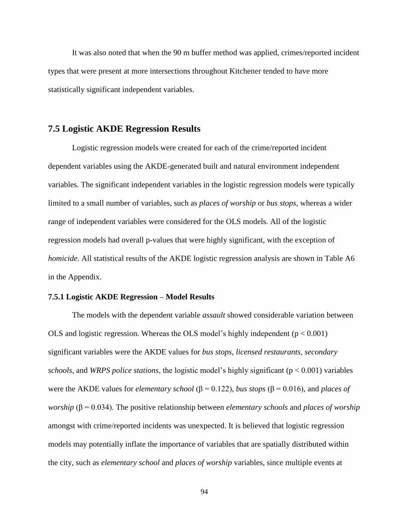
94
It was also noted that when the 90 m buffer method was applied, crimes/reported incident
types that were present at more intersections throughout Kitchener tended to have more
statistically significant independent variables.
7.5 Logistic AKDE Regression Results
Logistic regression models were created for each of the crime/reported incident
dependent variables using the AKDE-generated built and natural environment independent
variables. The significant independent variables in the logistic regression models were typically
limited to a small number of variables, such as places of worship or bus stops, whereas a wider
range of independent variables were considered for the OLS models. All of the logistic
regression models had overall p-values that were highly significant, with the exception of
homicide. All statistical results of the AKDE logistic regression analysis are shown in Table A6
in the Appendix.
7.5.1 Logistic AKDE Regression – Model Results
The models with the dependent variable assault showed considerable variation between
OLS and logistic regression. Whereas the OLS model’s highly independent (p < 0.001)
significant variables were the AKDE values for bus stops, licensed restaurants, secondary
schools, and WRPS police stations, the logistic model’s highly significant (p < 0.001) variables
were the AKDE values for elementary school (β = 0.122), bus stops (β = 0.016), and places of
worship (β = 0.034). The positive relationship between elementary schools and places of worship
amongst with crime/reported incidents was unexpected. It is believed that logistic regression
models may potentially inflate the importance of variables that are spatially distributed within
the city, such as elementary school and places of worship variables, since multiple events at

95
single intersections were not taken into account. Since logistic regression models only consider
presence or absence of assault occurrences, more spatially distributed independent variables tend
to be more significant than those that are clustered in particular areas of town.
Both the OLS and logistic regression models for break and enter identified bus stops (β =
0.011 in logistic regression) as highly significant (p < 0.001), and WRPS police stations (β =
0.206 in logistic regression) as moderately significant (p < 0.05). Places of worship (β = 0.033)
was highly significant (p < 0.001) and positively related to crime/reported incidents, but this is
likely due to lack of multiple crime/reported incident events occurring at single intersections.
This may also be due to more widespread occurrences of break and enter throughout the city
compared to other types of crime/reported incidents, which may result in a more significant
relationship with the distribution of churches. The dispute logistic regression model proved to be
quite similar to the break and enter logistic regression model results with similar chi-squared
values (87.309 for break and enter and 118.739 for dispute), and both identified only bus stops
(β = 0.016) and places of worship (β = 0.023) as significant (p < 0.01) independent variables. It
is unlikely that these two variables are highly related to each other and similar relationships are
likely due to similar spatial distributions when represented by a binomial variable in logistic
regression models.
The disturbance logistic regression model results were similar to the OLS model,
although places of worship (β = 0.037) was identified as highly significant (p < 0.001) and
positively related, while the OLS model identified universities as a highly significant (p < 0.001)
independent variable. This finding was unexpected, since one would tend to associate
universities with disturbances compared to religious institutions.

96
The logistic regression model for domestic disturbance appeared to be better fitting than
the corresponding OLS model. The OLS model identified bus stop (β = 0.014 in logistic
regression) as a highly significant independent variable. The logistic regression model, however,
also identified places of worship (β = 0.039) and the two school type variables (elementary
schools (β = 0.058) and secondary schools (β = 0.17)) as significant (p < 0.01). It is likely that
the more residential nature and broad spatial distribution of this crime/reported incident type
lends itself to logistic regression analysis.
The drugs logistic regression model was similar to its corresponding OLS model, as both
identified secondary school (β = 0.218 in logistic regression), licensed restaurants (β = 0.008 in
logistic regression), and GRT bus stops (β = 0.021 in logistic regression) as significant (p <
0.01). However, only the OLS model tested police stations to be highly significant (p < 0.001),
and only the logistic model identified places of worship (β = 0.036) as highly significant (p <
0.001). The positive and highly significant nature of these relationships was unexpected and as in
the case of many of the AKDE logistic regression models.
The logistic regression model based on AKDE buffers was the weakest for homicide. It
was the only model that was not highly significant overall, resulting in the smallest chi-squared
value (χ2 = 20.185). This is likely due to the fact that only nine homicides were recorded in
Kitchener-Waterloo during the study year. Unlike the OLS regression model of homicide, the
logistic regression model identified places of worship (β = 0.120) as a highly significant (p <
0.001) independent variable. This is an unexpected result, since one would not normally
associate homicide with places of worship, thus the statistical relationship was likely due to the
spatial distribution of a small recorded number of homicide cases.

97
The logistic regression model of impaired driver as the dependent variable was similar to
the corresponding OLS model, with both identifying licensed restaurants (β = 0.010 in logistic
regression) and LCBO and Beer Store locations (β = 0.206 in logistic regression) as highly
significant (p < 0.001) independent variables. Since both are alcohol-related independent
variables, this significant relationship was expected. The main difference between both models
was that only the OLS model tested universities as being a significant (p < 0.01) independent
variable, whereas only the logistic regression model tested bus stops (β = 0.009) as significant (p
< 0.01). The wide spatial distribution of bus stops in Kitchener-Waterloo likely contributed to the
significant logistic regression model.
Intoxicated person resulted in the largest chi-squared value of all tested logistic
regression models based on the AKDE buffer method (χ2 = 422.680). Both logistic and OLS
regression models considered bus stops (β = 0.026 in logistic regression) and licensed
restaurants (β = 0.011 in logistic regression) as highly significant (p < 0.001) independent
variables. Interestingly, LCBO and Beer Store locations (β = 0.206) was highly significant (p <
0.001) in the logistic regression model, as was expected due to the natural association between
alcohol sales and intoxication, despite not testing to be significant in the OLS model. Moreover,
unlike the OLS model, the logistic regression model did not identify universities or police
stations as significant independent variables, but places of worship tested to be significant (p <
0.01). Any crime/reported incident associated with the universities occurred at a small number of
intersections, likely accounting for the weaker relationship of this variable in logistic regression
model. The significant variables for the motor vehicle collision logistic regression model were
different than for the corresponding OLS regression model. However, bus stops (β = 0.019 in
logistic regression), licensed restaurants (β = 0.014 in logistic regression), places of worship (β

98
= 0.025 in logistic regression), and secondary schools (β = 0.157 in logistic regression) were
significant (p < 0.05) in both models.
More significant independent variables were identified in the logistic regression model of
property damage than in the OLS regression model. The OLS model tested police stations (β =
0.185 in logistic regression), licensed restaurants (β = 0.006 in logistic regression), and bus stops
(β = 0.013 in logistic regression) as significant variables (p < 0.05), but the logistic regression
model also identified elementary schools (β = 0.077), bus stops (β = 0.013), and secondary
schools (β = 0.192) as highly significant (p < 0.001) and places of worship (β = 0.018) as
moderately significant (p < 0.05) variables. It is likely that the well-distributed nature of this
crime/reported incident type contributed to the increased number of significant variables in the
logistic regression model, for reasons previously discussed.
The logistic regression model proved to be a better fit for prostitution compared to the
OLS regression model. Both identified places of worship (β = 0.124, in logistic regression) as
highly significant (p < 0.001) and the logistic regression model identified bus stops (β = 0.011)
and police stations (β = 0.352) as moderately significant (p < 0.05). Again, this dependent
variable had a low recorded number of occurrences of this crime/reported incident type, which
likely contributed to the model’s poor goodness of fit. Also, as previously discussed, prostitution
might be difficult to model, due to the fact that more than one location could potentially be
linked to an individual crime/reported incident. Robbery, a dependent variable with a similarly
low number of occurrences of this crime/reported incident type, was better fitting in the OLS
regression model compared to the logistic regression model. Both identified secondary school (β
= 0.319, in logistic regression) and bus stops (β = 0.015, in logistic regression) as highly
significant (p < 0.001), but the OLS model also identified LCBO and Beer Store locations,

99
licensed restaurants, and universities as significant (p < 0.05) variables. Since robbery is more
concentrated in downtown locations, it was expected that OLS regression would yield a superior
model in comparison to a logistic regression model specification.
Both OLS and logistic regression models of sex offence/indecent act identified bus stops
(β = 0.016, in logistic regression) and secondary school (β = 0.229, in logistic regression) as
significant (p < 0.01) independent variables. Similarly, few variables were identified as
significant in regression models of suspicious person or vehicle. Both identified places of
worship (β = 0.044, in logistic regression) and bus stops (β = 0.012, in logistic regression) as
significant (p < 0.01), although the logistic regression model also yielded elementary school (β =
0.067) as a significant (p < 0.01) independent variable. This is likely due to the wide spatial
distribution of this variable. Theft motor vehicle also resulted in weak regression models with bus
stops (β = 0.012) and police stations identified as the only highly significant (p < 0.001)
variables in the logistic and OLS regression models, respectively. The lack of fit for both models
may be due to the fact that criminals who steal cars may be distributed throughout the city or else
criminals themselves may pick random targets.
The logistic regression model for theft under $5,000 yielded more significant variables
than the corresponding OLS regression model. While the OLS model only identified three
significant (p < 0.05) variables, the logistic regression model resulted in seven significant
variables, likely due to the large number of this crime/reported incident type in Kitchener-
Waterloo. Also, theft under $5,000 occurred at many street intersections throughout the city.
Again, universities, where thefts were generally known to occur, was not a significant
independent variable.

100
The two unwanted person models yielded similar results with bus stops (β = 0.020, in
logistic regression), licensed restaurants (β = 0.013, in logistic regression), and places of
worship (β = 0.057, in logistic regression) as highly significant (p < 0.001), and secondary
school (β = 0.132, in logistic regression) and universities (β = 0.304, in logistic regression) as
moderately significant (p < 0.05). Some independent variables were moderately significant in
one model but not the other, while LCBO and Beer Store (β = 0.134) locations tested to be
significant (p < 0.01) in the logistic regression model.
7.5.2 Logistic AKDE Regression – Independent Variable Results
The results of the logistic regression ADKE models are shown in Table A6 of the
Appendix. The elementary school AKDE value was a well-fitting independent variable in the
logistic regression model. Elementary schools was also an unexpectedly positive coefficient in
all logistic regression models where it was significant (p < 0.05). As with other variables
associated with residential areas, the greater significance of elementary schools in the logistic
regression model was likely due to the use of binomial dependent variables, which eliminated
multiple events at street intersections and aggregated observations into presence and absence
indicators. As previously noted, this reduced the influence of the higher number of
crime/reported incidents at downtown intersections, which potentially inflates the importance of
independent variables that are not concentrated in the downtown core.
The bus stops AKDE value was the best fitting variable in both logistic and OLS
regression results and it was significant (p < 0.05) in all but one logistic regression model, and all
but four OLS regression models. Bus stops was also a highly significant (p < 0.001) predictor for
fifteen types of crime/reported incidents, while it tested significant for twelve crime/reported
incident types when OLS regression models were used. As previously mentioned, this was

101
expected to be a strong variable, since bus stops provide an outdoor location where individuals
wait alone or in small numbers, and could make them more susceptible to crime, in accordance
with Routine Activity Theory (Cohen & Felson, 1979). However, it is also believed that the wide
spatial distribution of bus stops could contribute to inflating the importance of this variable in
logistic regression models. A large number of bus stops are located downtown, while fewer are
located in suburban areas and throughout the rest of the city. There are also typically two bus
stop locations at each intersection when they are present (one on each side of the street). For
these reasons, it is possible that the bus stop AKDE value’s statistical correlation was inflated
due to its spatial distribution, or lack of spatial concentration of the binomial crime/reported
incident dependent variables in downtown areas.
Hospitals was one of the weakest fitting independent variables in both the logistic and
OLS regression models. It was only significant (p < 0.05) for one crime/reported incident type
(drugs) when logistic regression models were estimated and did not test to be significant in OLS
regression models. As previously mentioned, this finding was expected, since there are very few
hospitals located in the region. The LCBO and Beer Store AKDE values were similarly weak in
significance when both logistic and OLS regression models were tested. The variable was
significant (p <0.05) in six and five of the logistic and OLS regression models respectively,
although it was more significant amongst the OLS regression models tested. As previously
mentioned, this is likely due to the wider distribution of this variable, since both organizations
have stores fairly evenly distributed throughout the study area to increase accessibility to
residents and potential customers. As expected, this variable tested to be highly significant (p <
0.001) in the intoxicated person logistic regression model due to the link between alcohol and
intoxication, although interestingly, it did not test to be significant in the OLS regression model.

102
Similar to the previous two independent variables, the ADKE values of libraries,
community centre, and arenas tested to be weak in both logistic and OLS regression models. It
was only moderately significant (p < 0.05) in two logistic regression models and in three OLS
models. Similar to the hospitals variables, libraries, community centre, and arenas was not
expected to be a well-fitting variable. It demonstrated a positive relationship with crime/reported
incident types in both regression methods.
The licensed restaurants AKDE values tested to be slightly more significant in OLS
regression when compared to logistic regression results. In logistic regression, the variable was
significant (p < 0.05) in nine models and highly significant in six, whereas in OLS regression, it
was significant in eleven models and highly significant (p < 0.001) in seven. The AKDE values
were significant with many of the same dependent variables, including many of those thought to
be associated with alcohol consumption. Both regression models showed that licensed
restaurants was consistently a good predictor of crime/reported incidents.
The places of worship AKDE values tended to be more significant predictors in logistic
regression model results. Although the variable was only significant (p < 0.05) in five of the
OLS regression models, it tested to be significant (p < 0.05) in fifteen of the logistic regression
models. It was also a positive coefficient in every logistic regression model. As previously noted,
the significance of the places of worship variable is believed to be due to the broad spatial
distribution of churches throughout Kitchener-Waterloo, with a number of older churches
concentrated in the downtown core, and many other churches scattered throughout the city. This
spatial distribution is similar to the spatial pattern of the binomial data for many crime/reported
incident types, which might lead to the false notion of churches being a key factor in the
presence or absence of crime.

103
The secondary schools AKDE values had a similar significance in both logistic and OLS
regression models. The fit of the ADKE values for universities in logistic regression was poor in
comparison to the OLS regression results. The variable was only significant (p < 0.05) once in
the logistic regression models, compared to six models where it was significant (p < 0.05) in
OLS regression results. This is likely because many of the crime/reported incidents on each
university campus were relocated to a small number of intersections adjacent to the institutions,
which are represented as single events by the binomial variables. This also appears to be the case
with the AKDE values for WRPS police stations in the logistic regression model. Although the
variable was significant in five models in logistic regression analysis, it tested to be only
moderately significant (p < 0.05). Again, this is likely due to most crime/reported incidents in
and around police stations being tagged to a small number of surrounding street intersections,
which would be treated like single events in the logistic regression analysis.
7.5.3 Logistic AKDE Regression Results – Summary of Key Findings
The results of AKDE logistic regression models identified bus stops and alcohol licenses
as significant independent variables. However, places of worship unexpectedly tested to be
significant in all but three logistic regression models and always had a positive coefficient. This
was likely a misleading result caused by the spatial pattern and clustering of churches (e.g., a
concentration of older churches downtown with others scattered throughout suburban residential
areas) coincidentally matching the pattern of many presence/absence crime/reported incident
variables. While secondary schools also tested to be a significant predictor of crime incidents,
universities and police stations were rarely significant in tested logistic regression models. In the
case of universities, the lack of significance is likely due to the fact that crime/reported incidents

104
committed at universities were usually aggregated at the closest intersections, thus obscuring
potential statistical relationships.
7.6 NDVI Analysis Results
The intent of this section is to evaluate which crime types are most strongly associated
with levels of vegetation cover, while recognizing that this relationship may be directly or
indirectly linked with the presence or absence of vegetation. As noted in Section 6.3, regression
models were tested where NDVI was considered as the dependent variable, and crime/reported
incidents were the independent variables, simply to assess the strength of relationships between
the sets of variables.
Results of this analysis provided further evidence of statistical relationships between
crime and its surrounding environment. When the crime/reported incident variables were
significant, these relationships were most often negatively related to vegetation. This is
consistent with the findings of Wolfe and Mennis (2012) which indicated that abundant
vegetation was associated with decreased rates of various crime types. This likely indicates that
crime/reported incidents are more common in areas of low vegetation where concrete and asphalt
landcover and building roofs are more common, such as downtown areas. Independent variables
that tested to be highly significant include motor vehicle collision and intoxicated person. Other
variables, including break and enter and homicide were rarely or never significant within the
tested models. Results of the eight NDVI models are provided in Table 5, which shows the
significance levels and coefficients for each crime/reported incident type in each of the models
tested.

105
Table 5. Results of eight regression models tested in the analysis of NDVI and crime/reported
incidents. “***” represents a p-value below 0.001, “**” represents a p-value below 0.01 but
above 0.001, and “*” represents a p-value below 0.05 but above 0.01.
Number of Crime/Reported Incidents Crime/Reported Incidents Presence/Absence
90 m Adaptive 90 m Adaptive
Mean Maximum Mean Maximum Mean Maximum Mean Maximum
Intercept 0.232 *** 0.392 *** 0.228 *** 0.365 *** 0.237 *** 0.391 *** 0.235 *** 0.371 ***
Assault 0.000 0.000 0.000 0.001 -0.002 0.004 -0.002 -0.002
Break and
enter -0.003 * 0.001 -0.002 -0.001 0.003 0.010 * 0.003 0.004
Dispute 0.001 0.001 0.001 0.000 0.002 0.005 0.002 -0.002
Disturbance -0.002 * -0.004 ** -0.002 -0.004 ** -0.010 ** -0.016 ** -0.011 ** -0.014 **
Domestic
dispute 0.001 0.002 ** 0.000 0.000 0.003 0.004 0.002 -0.002
Drugs -0.002 -0.001 -0.001 0.000 -0.013 *** -0.014 ** -0.012 *** -0.011 *
Homicide -0.025 -0.048 -0.021 -0.041 -0.013 -0.043 -0.009 -0.034
Impaired
driver -0.001 0.009 * -0.004 0.001 -0.005 0.016 * -0.007 0.004
Intoxicated
person -0.002 * -0.006 *** -0.003 * -0.004 * -0.018 *** -0.024 *** -0.018 *** -0.018 ***
MVC -0.001 *** 0.000 -0.002 *** -0.001 ** -0.013 *** -0.001 -0.014 *** -0.007 *
Property
damage -0.001 0.001 -0.001 -0.001 0.001 0.009 * -0.002 -0.002
Prostitution -0.004 ** -0.003 -0.004 ** -0.002 -0.032 *** -0.047 *** -0.026 *** -0.011
Robbery -0.005 -0.009 -0.002 -0.005 -0.012 * -0.018 -0.010 -0.011
Sex offence
indecent act 0.003 0.010 * 0.000 0.003 0.004 0.008 0.000 0.005
Suspicious
person or
vehicle 0.003 ** 0.006 ** 0.002 0.004 * 0.008 *** 0.011 ** 0.006 * 0.006 *
Theft motor
vehicle -0.001 0.000 -0.001 -0.002 * -0.002 0.005 -0.004 0.000
Theft under
$5,000
dollars -0.001 *** -0.001 ** -0.001 *** -0.001 *** 0.003 0.006 0.003 0.001
Unwanted
person -0.001 *** -0.002 *** -0.001 *** -0.001 ** -0.017 *** -0.017 *** -0.017 *** -0.017 ***
Assault and dispute resulted in some of the smallest coefficients observed in the NDVI
models that were tested. Moreover, both crime/reported incident types had the least significant
relationships with vegetation, not testing to be significant in any of the eight models considered.

106
Homicide was also not significantly associated with NDVI. However, this is likely due to the
very low number of homicide events reported. Break and enter also tested to be not significantly
related to NDVI, being only moderately significant in two of the models tested. It is possible that
break and enter occurrences were more well distributed throughout the city and thus, randomly
associated with vegetation cover.
Disturbance tested to be significantly related with NDVI in all but one regression model
and was negatively related to vegetation. Domestic disturbance was only significant in one of the
tested models for NDVI. It is possible that domestic disturbance is similar to break and enter,
since its occurrences are well distributed geographically and therefore associating randomly with
vegetation levels.
The relationship between drugs and vegetation was quite unusual. It tested to be
significant and negative in four models where the presence/absence crime/reported incident
variables were tested, but was not significant in four models where count crime/reported incident
variables were tested. Homicide was one of the least significant independent variables tested in
the NDVI analysis. As previously mentioned, this is likely due to the low number of homicides
reported in Kitchener-Waterloo. Impaired driver was also identified as not significant. This is
likely that the locations where persons are stopped for impaired driving are well distributed,
because the offenders are in automobiles and highly mobile, which reduces the potential for a
strong spatial relationship with vegetation cover.
Intoxicated person was one of the most significant variables tested in eight models of
NDVI as the dependent variable. The relationship tested to be negative, suggesting that alcohol-
licensed establishments are usually located in low vegetation covered areas, such as downtown
or in suburban commercial centres where concrete and asphalt cover are abundant. It is also

107
interesting to note that four of the five models in which this variable tested to be highly
significant were models where presence/absence crime/reported incident variables were used.
The coefficients for intoxicated person were negative and larger when presence/absence
crime/reported incident variables were used. This might be due to the fact that presence/absence
of a crime/reported incident type correlates better with vegetation than with counts for the
crime/reported incident type, as presence/absence variables better match the limited variation of
NDVI values. Motor vehicle collision was also one of the more significant variables tested in the
eight models shown in Table 5. It was significant in six of the eight models, and highly
significant in four. Also notable is that motor vehicle collision resulted in a negative coefficient
in all models, verifying that areas where vehicle collisions occur will be on roads and high
asphalt covered areas, corresponding to low NDVI valued. Busier roads are also larger and tend
to be associated with more accidents.
Property damage was not significant in NDVI models. This is likely due to the well
distributed nature of this crime/reported incident type, resulting in its occurrence at a number of
intersections with diverse vegetation cover, being widely spread geographically. Unexpectedly,
prostitution was identified as a significant variable and negatively related to NDVI. This
indicates that if vegetation cover had been included as an additional variable in the buffer and
AKDE models predicting crime/reported incidents, model fit could have potentially improved.
Robbery and sex offence/indecent act tested to be significant in only one model likely due
to the low number of cases reported in the city. Suspicious person or vehicle tested to be
significant in seven of the eight models of NDVI and one of the only relationships that was
positive. It is possible that this positive relationship is due to a tendency for suspicious people to
hide near vegetation cover. Contrary to other results of this analysis, these results may support

108
the theory put forward by some studies that vegetation aids criminals, as it may be used to hide
their activities (Nasar & Fisher, 1993; Michael, et al., 2001).
Theft motor vehicle was not significantly related to NDVI, likely due to its moderately
small count of reported events. Results of theft under $5,000 were similar but negatively related
to NDVI. However, a significant relationship was not detected when presence/absence
crime/reported incident variables were.
Unwanted person consistently tested as being significantly related to NDVI or vegetation
cover and was identified as a significant variable in all eight models. In models tested in previous
sections and also with NDVI, the results of unwanted person were consistently similar to
reported cases of intoxicated person. In summary, all crime/reported incidents involving
undesirable people or behaviour (e.g., intoxicated person, suspicious person or vehicle, and
unwanted person) tested to be significantly related to NDVI, whether those relationships were
positive or negative. This suggests that vegetation cover may play a role in where deviant
behaviour occurs or persists spatially within Kitchener-Waterloo.

109
8.0 Discussion
The primary goal of this study was to explore the relationship between crime/reported
incidents and the built and natural environment in the cities of Kitchener and Waterloo, Ontario.
The models tested to study this relationship, using multiple methods and datasets, proved to be
weak with low r-squared values. This would suggest the relationship between the built and
natural environment is also weak. The secondary goal was to determine which built and natural
environment features had the strongest relationships with each type of crime/reported incident.
Bus stops were found to have the most significant relationship with crime/reported incidents,
being identified as significant with the majority of crime/reported incident types. Since bus stops
attract large numbers of individuals, this likely creates opportunities for potential criminal
activity. Alcohol licensed facilities also resulted in a significant relationship with crime/reported
incidents. Certain types of crime/reported incidents, such as intoxicated person or assault may be
directly or indirectly related to alcohol. Streetlighting was significant in some models but its
positive relationship with crime/reported incidents was unexpected as it was expected to be
crime deterrent. It was likely that, similar to bus stops, streetlighting attracts individuals during
night time hours who wish to travel in a lit area, thus creating criminal opportunity. Commercial
buildings, secondary schools, and universities all showed significance with several
crime/reported incident types, particularly crime types that are often associated with the three
buildings types (e.g. theft with commercial buildings, disturbances with both universities and
secondary schools). Commercial residential buildings and institutional buildings both were also
significant with several crime/reported incident types, though this was likely because of their
spatial concentration downtown rather than any relationship those building types had with crime.
The relationship between crime/reported incidents and the natural environment also appeared

110
weak from initial tests. However, a negative relationship did appear to exist between several
crime/reported incident types and NDVI values, as well as a positive relationship between
suspicious person or vehicle and NDVI values.
8.1 Buffer and AKDE Methods
Overall, neither the static and adaptive buffer nor AKDE methodologies produced very
strong OLS regression models of built/natural environmental predictors of crime/reported
incidents, with the largest r-squared value being 0.227. Several models resulted in r-squared
values above 0.1, but most models were weak with r-squared values below 0.1. These findings
imply a weak relationship of built/natural environmental features with crime/reported incidents,
which could be due to several possible reasons. A likely reason is missing variables, such as
socio-economic factors that were not considered in the regression models in this study. It was
initially believed that since Kitchener-Waterloo is a moderately-sized urban area, the relatively
consistent socio-economic status of neighbourhoods within the city would not have a significant
effect on crime. This assumption was partly due to short distances between neighbourhoods of
varying socio-economic status, allowing for easy travel and greater connectivity, unlike in larger
cities. Moreover, it was difficult to compare socio-economic data and crime/reported incidents in
this study, since socio-economic data are recorded at aggregate units of different sizes and
shapes, such as census tracts or dissemination areas, which would be challenging to compare
with street intersection points to which crime/reported incidents were assigned, without
committing an ecological fallacy (Tranmer & Steel, 1998). If socio-economic data for census
polygons were assigned to street intersections at which crime/reported incidents were identified,
it is likely that many intersections located close together would have been assigned with the

111
same socioeconomic characteristics. Nevertheless, comparison of socio-economic variables and
including them in the regression models may form an additional dimension to this work and
potentially improve the model fit by including additional variables.
Furthermore, it is possible that some statistically significant relationships between
built/natural environment variables and crime/reported incidents could have been an artifact of
the data that were collected and considered to be indicators representative of human activity,
rather than being factors in determining the locations of crime. This is particularly the case with
bus stops, which was identified as a highly significant variable in this study for predicting
crime/reported incidents. It is known that bus stops tend to be associated with areas of high
activity, transit, and gathering of people, associated with demands for public transportation. This
observation is consistent with the concept of ‘crime generators’ proposed by Brantingham and
Brantingham (1995), which states that places that attract large numbers of people can become
generators of crime. Brantingham and Brantingham (1995) specifically mention that “bus
interchanges, transit system stops, [and] massive park and ride parking lots can all become crime
generators because of the volumes of people that pass through them” (p. 7). Therefore, although
built environment features such as bus stops might be more related to human activity than crime
itself, crime in many respects is tied to human activity, and bus stops represent congregation
points for people. These observations are also consistent with Cohen and Felson’s (1979)
Routine Activity Theory. This theory states that crime occurs when motivated offenders, suitable
targets, and a lack of guardianship converge in a particular time and space. As bus stops attract
large numbers of people intent on using transit, this provides motivated offenders with numerous
suitable targets for their criminal activity.

112
Another weakness identified in this study was that building and land uses are not
randomly distributed in Kitchener-Waterloo. Certain built environment features and factors, such
as percentage institutional, had high concentration of facilities located in downtown areas and
such spatial patterns are not necessarily related to crime, but attributed to economics and other
human-related activities and processes. It is believed that although the corresponding regression
models may have been significant, such relationships are likely inflated in significance due to
spatial patterns, population, and other factors that are not related to crime. Future research may
explore how to adjust for spatial effects and spatial autocorrelation in the datasets and to isolate
urban/built environment effects on crime.
When the performance of the buffer method and the AKDE method were compared, the
buffer method was the preferred overall methodology. The buffer method resulted in higher r-
squared values with the majority of dependent crime/reported incident variables. The buffer
method’s better performance may have been due to its independent variables being generally
superior to those tested in the AKDE method. The AKDE analysis required point data for built
environment features in order to create the necessary AKDE rasters. However, available datasets
of building use types were quite limited in point form, since only specific datasets were provided
mainly by government sources and developed for specific applications. This also entailed that an
excessive number of government facilities were often represented as independent variables in the
AKDE models. Although some business registry datasets were available, these were difficult to
classify and other flaws or errors were often apparent (e.g., lack of chain stores and restaurants,
containing home businesses). Inclusion of business registry points as rasters within the AKDE
models, even if unclassified, could potentially improve overall model performance. Nevertheless,
the buffer methodology applied in this study was able to utilize the building footprint dataset,

113
which provided a classification of each building within the city. Although this classification
could be further divided into more sub classes, this methodology still enabled representation of
the built environment to be captured within the dataset of Kitchener’s building footprints.
The adaptive buffer method was determined to have superior performance to the 90 m
static buffer method in this study. Regression models based on adaptive buffers resulted in
overall higher r-squared values when considering the same set of dependent variables. Basing the
buffer radius on the distance to the four nearest intersections appeared to better represent the
individual built and natural environment at each street intersection, therefore making it the
superior methodology than a static buffer representing all street intersections of the study area
with the same radius.
When logistic and OLS regression methods were compared, the OLS regression model
was considered to be the best in terms of goodness of fit and more statistically significant
independent variables. The AKDE logistic regression analysis also indicated places of worship
as a significant variable and positively related to crime/reported incidents, which ran counter to
expectations. Such significant relationships tested from logistic regression models was likely
due to the similar spatial distribution of churches (e.g., a small cluster of churches located
downtown with other churches distributed throughout the study area) with the spatial distribution
of crime/reported incident dependent variables, which only considered presence/absence rather
than the number of incidents. This demonstrated the tendency of AKDE logistic regression
models to result in false positive conclusions by not accounting for crime/reported incident
counts and focusing only on presence/absence of cases. The OLS regression methodology was
judged to be superior for this analysis, since it resulted in identifying fewer false positives.
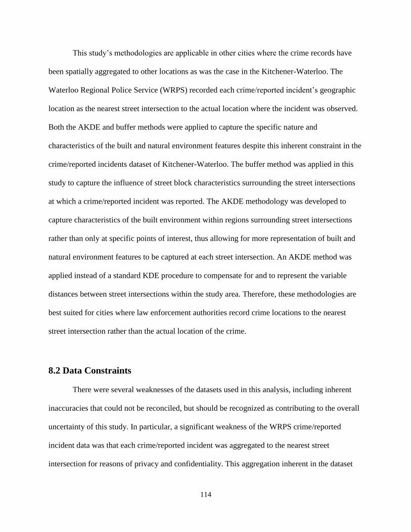
114
This study’s methodologies are applicable in other cities where the crime records have
been spatially aggregated to other locations as was the case in the Kitchener-Waterloo. The
Waterloo Regional Police Service (WRPS) recorded each crime/reported incident’s geographic
location as the nearest street intersection to the actual location where the incident was observed.
Both the AKDE and buffer methods were applied to capture the specific nature and
characteristics of the built and natural environment features despite this inherent constraint in the
crime/reported incidents dataset of Kitchener-Waterloo. The buffer method was applied in this
study to capture the influence of street block characteristics surrounding the street intersections
at which a crime/reported incident was reported. The AKDE methodology was developed to
capture characteristics of the built environment within regions surrounding street intersections
rather than only at specific points of interest, thus allowing for more representation of built and
natural environment features to be captured at each street intersection. An AKDE method was
applied instead of a standard KDE procedure to compensate for and to represent the variable
distances between street intersections within the study area. Therefore, these methodologies are
best suited for cities where law enforcement authorities record crime locations to the nearest
street intersection rather than the actual location of the crime.
8.2 Data Constraints
There were several weaknesses of the datasets used in this analysis, including inherent
inaccuracies that could not be reconciled, but should be recognized as contributing to the overall
uncertainty of this study. In particular, a significant weakness of the WRPS crime/reported
incident data was that each crime/reported incident was aggregated to the nearest street
intersection for reasons of privacy and confidentiality. This aggregation inherent in the dataset

115
results in uncertainty in the exact location of crime/reported incidents represented in this study,
especially for areas with longer street segments or wide spaced street intersections, such as rural
or suburban regions. Moreover, a substantial number of crime/reported incent records did not
have geographic location information available and were not possible to geocode in the study’s
dataset, which were ultimately eliminated from the dataset and thus excluded from the analysis.
It is possible that a number of notable, actual crimes were excluded from this study due to the
lack of spatial information attached to them. However, it was not known why locational
information was missing for certain incidents and this could very well be reflective of incidents
that the WRPS did not consider worthwhile to further investigate or did not have sufficient
information to record in the database.
Errors were also occasionally identified within the crime/reported incidents dataset.
While some built feature datasets, such as alcohol establishment data, where inspected in detail
by the author on a record-by-record basis for accuracy, the WRPS crime/reported incident
dataset was very large and it was not possible to verify whether all of the information related to
each crime/reported incident was correct. Based on the results reported from this study,
significant errors were not apparent and model analysis results could either be explained or were
within expectations. Therefore, significant errors were not immediately apparent despite the
inherent uncertainty related to the datasets used in this study.
Another weakness of this study was the temporal misalignment of datasets used in this
analysis. For example, both the crime/reported incident dataset and Landsat 8 image were from
2013, but the alcohol license dataset was obtained for 2014. The weakness of temporal
misalignment was not considered to have significantly negative effect on the results of this study,

116
since the vast majority of built environment features in Kitchener-Waterloo would not change
drastically from year to year.
There was also the potential for differences or inconsistencies between the street
intersection dataset acquired and used in this study, and the maps and approaches used by
individual WRPS police officers to register monitored crime/reported incidents to the closest
street intersections. As previously discussed, each intersection was created in this study using the
“Intersect” tool in ArcGIS on a roads layer sourced from the Ontario government. Each
intersection created by this process was individually inspected by the author and. intersections
were eliminated if they were not included in the WRPS crime/reported incident dataset.
Eliminated road segments included cul-de-sacs, underpasses, duplicate intersection on roads with
medians, and new housing developments that lacked criminal activity. Despite detailed
inspection of this dataset by the author, it is still nevertheless likely that inconsistencies may still
exist and that both datasets do not match exactly. For example, it is possible that some street
intersections in new housing developments were excluded, which the WRPS might have
considered to be active intersections.
8.3 Comparison to Previous Research
This study found that alcohol facilities were significantly and positively associated with
crime/reported incidents, with the exception of the logistic regression model based on 90 m
buffers. This finding is consistent with existing literature (e.g., Day et al., 2012; Kumar &
Walyor, 2003), which found that alcohol establishments are a significant factor in the spatial
distribution of crime within urban areas. Moreover, many of the models tested in this study
resulted in high r-squared values when linked to alcohol, including intoxicated person and

117
disturbance. However, when liquor stores were examined on their own, minor effects were
observed.
There are conflicting findings concerning the relationship between transit stops and crime
in the literature. For example, Barnum et al. (2017) identified a positive relationship between
transit stops and crime incidents in all three cities that were studied, while Sohn (2016) found a
negative relationship. The results from this study support those by Barnum et al. (2017),
suggesting that more crime tends to occur around bus transit stops within a city.
Likewise, the relationship between vegetation and crime has been debated in existing
literature, with some studies determining a negative relationship (Wolfe & Mennis, 2012; Chen,
et al., 2005), while others conclude that the relationship is positive (DeMotto & Davies, 2006).
The results from this study supports the former opinion. Although the buffer analysis results
determined that parks and golf courses were an insignificant factor, the analysis of NDVI data
values suggests that vegetation has a significant and negative relationship with several types of
crime/reported incidents, such as intoxicated person and prostitution. Therefore, this study tends
to support the theory that vegetation can act as a crime deterrence and perhaps lead to ‘mental
softening’ that subsequently decreases crime rates (Kaplan, 1987). The presence of vegetation
cover may encourage citizens to provide informal surveillance (Jacobs, 1961) and may be related
to theories of social capital and collective efficacy. Community members who tend to be active
outside tend to enjoy vegetation, greenspace, and recreation areas, and would be more likely to
report suspicious or criminal behaviour than compared to community members who stay indoors
or are less involved with their local community. Suspicious person or vehicle was the only
crime/reported incident variable that tested to have a significant and positive relationship with
NDVI values. This demonstrates that the nature of this crime type might lend itself to a positive

118
relationship with vegetation, since vegetation may provide opportunities for crime perpetrators to
hide and reduce their visibility. In the case of suspicious persons, hiding behind vegetation may
be a common reason why these individuals appear suspicious to members of public.
In analysing the finding of this study, it is important to remember the findings of Barnum
et al. (2017), who conducted Risk Terrain Modelling (RTM) analysis on three cities using the
same variables as this study and determined inconsistencies in the significant relationships of
urban environment features as predictors of crime. Using the analogy of a kaleidoscope, Barnum
et al. (2017) suggested that the arrangement of urban features within a city can affect how crime
is distributed within a city, thus making the crime risk factors associated with urban features
unique in each city. This analogy would apply to Kitchener-Waterloo, as evidenced by the results
of this study. It is likely that various factors, including the cities’ size and urban design interact
and affect relationships between various types of crime/reported incidents and feature of the built
and natural environment in urban areas.
8.4 Significance of Research Findings
There are potential real-world applications of this research, particularly in law
enforcement. Knowing where crimes are more likely to occur can be useful in planning of patrol
routes and targeting policing efforts. Patrol routes could be designed so areas with a large
numbers of urban features identified as ‘crime attractors’ and/or ‘crime generators’ (e.g., bus
stops, streetlights) in this study can be properly patrolled by police cars. Areas with substantial
concentrations of crime prone environment features could be identified as areas suited for foot
patrols. These models could further be used to assess potential crime levels at new commercial
and/or residential developments as part of their site assessment plans. This assessment essentially

119
only requires knowledge of the building development’s use and transportation and general
infrastructure information in its proximity. The models tested in this study may be applied to
assess the level of crime that could potentially be introduced into an area by new development.
This study’s results could have potential implications in zoning practices in city planning.
This is particularly important when considering alcohol selling establishments, which were
identified in this study as a potential ‘crime attractor’ and an important environmental factor in
predicting crime and reported incidents. It is important for zoning laws to ensure that ‘crime
attractor’ building types and uses, such as alcohol selling establishments, are kept separate from
residential zoned areas. This may help with managing the spatial distribution of crime
occurrences and containing crimes within certain areas of the city.
This study adopted an exploratory approach when assessing the relationship between
crime and vegetation. Many crime and incident report types were significantly and negatively
related to vegetation, suggesting that there are lower crime levels in areas with more vegetation
cover. This suggests that one way of helping to alleviate crime is through the planting of
vegetation cover. Perhaps if more vegetation were to be planted and maintained in the cities of
Kitchener and Waterloo, levels of certain crime types could be reduced.

120
9.0 Conclusions
In conclusion, the models tested to study the relationship between crime/reported
incidents and the built and natural environment were quite weak with low r-squared values.
These results suggest a weak relationship between crime and the built and natural environment.
This also perhaps stresses the importance of including socio-economic factors and other
confounding variables when studying the spatial distribution of crime. It was found that bus
stops and alcohol licensed facilities were the built environment factors that were most associated
with crime/reported incidents and their spatial distribution within Kitchener-Waterloo, Ontario.
This positive relationship with crime/reported incidents was consistent among results from both
the buffer and AKDE methods. In future studies of crime and its relationship with the
environment, bus stops and alcohol licensed facilities are critical environment features to include
in such analyses. Bus stops’ positive and significant relationship with crime/reported incidents is
like due to bus stops being classified as ‘crime generators’, which attract people who could be
potential targets for offenders. Alcohol licensed facilities’ positive and significant relationship
with crime/reported incidents is likely due to its direct and indirect link with several crime types,
such as intoxicated person and assault. Streetlights was also an important factor and positively
related with crime/reported incidents, likely for similar reasons as bus stops as they attract
individuals at night who could be potential targets.
Most types of building uses were weakly associated with crime and reported incidents,
with some of the more significant being percentage institutional, percentage commercial,
percentage commercial residential, secondary schools and universities. It is suspected, however,
that some of these significant relationships of built environment features with crime/reported
incidents are at least partially explained by their spatial concentration in the downtown core.
121
Among the crime/reported incident variables that resulted in higher r-squared values were
intoxicated person, disturbance, unwanted person, assault, and drugs. These crime types,
therefore, may be the most spatially related to surrounding urban environment characteristics.
Several types of crime/reported incidents resulted in significant and negative relationships with
NDVI values or vegetation cover, supporting the conclusion that vegetation reduces crime levels.
Conversely, suspicious person or vehicle had a positive and significant relationship with NDVI
values.
Results of this study indicated that the buffer method was superior to the AKDE method,
since resulting regression models and more independent variables were significant. Also, the
adaptive buffer method was considered to be better than the 90 m static buffer approach and
produced stronger models in the majority of cases. Therefore, when all of the methodologies
tested in this study are considered, the adaptive buffer methodology is the recommended
approach for future studies on crime and built/natural environment relationships. Furthermore,
OLS regression was preferred over logistic regression analysis, since the OLS models resulted in
less false positives and better identified the importance of spatial concentrations in crime data.
Overall, the methodologies implemented in this study were ultimately constrained by available
crime datasets and the uncertainty associated with aggregating crime occurrences to the nearest
intersection. The methodologies applied in this study will be useful for conducting similar
studies in other Canadian cities that also record crime aggregated to the closest street intersection
and for exploring the relationship between such datasets with characteristics of the built and
natural environment.

122
Bibliography
Ackerman, W. V., & Murray, A. T., 2004. Assessing spatial patterns of crime in Lima, Ohio.
Cities, 21 (5), p. 423-437.
Adams, D., 2015. RE: Addition GIS data. [email] (Personal communication, 5 August 2015).
Alcohol and Gaming Commission of Ontario (AGCO) (n.d.). Requesting Information / FOI
Requests. [online] Available at: <http://www.agco.on.ca/en/contact/request_info.aspx>
Baddeley, A., 2016, October 13. Package ‘spatstat’. [online] Available at: <https://cran.r-
project.org/web/packages/spatstat/spatstat.pdf>
Barnum, J. D., Caplan, J. M., Kennedy, L. W., & Piza E. L., 2017. The crime kaleidoscope: A
cross-jurisdictional analysis of place features and crime in three urban environments.
Applied Geography, 79, p. 203-211.
Brantingham, P., & Brantingham, P., 1995. Criminality of place: Crime generators and crime
attractors. European Journal on Criminal Policy and Research, 3(3), p. 5-26.
Brinon, V., 2016. Crime data process in Waterloo region: Production of a geodatabase and
spatial analysis. [Internship report] École Nationale des Sciences Géographiques
Caplan, J. M., Kennedy, L. W., & Miller, J., 2011. Risk Terrain Modeling: Brokering
Criminological Theory and GIS Methods for Crime Forecasting. Justice Quarterly, 28(2),
p. 360-381.
Ceccato, V., & Dolmen, L., 2011. Crime in rural Sweden. Applied Geography, 31, p. 119-135.
Chen, D., Weeks, J. V., & Kaiser Jr.., J. V., 2005. Remote Sensing and Spatial Statistics as Tools
in Crime Analysis. Geographic Information Systems and Crime Analysis.
City of Kitchener, n.d.a. Open Data - Kitchener. [online] Available at:
<http://data.kitchenergis.opendata.arcgis.com/>

123
City of Kitchener, n.d.b. STREETLIGHTS. University of Waterloo Geospatial Centre [Accessed
16 December 2015]
City of Waterloo, n.d.a. City of Waterloo {OPENDATA}. [online] Available at: < http://opendata-
city-of-waterloo.opendata.arcgis.com/>
City of Waterloo, n.d.b. Recreation Facilities. [online] Available at:
<http://www.waterloo.ca/en/gettingactive/recreationfacilities.asp>
Cohen, E., & Felson, M., 1979. Social Change and Crime Rate Trends: A Routine Activity
Approach. American Sociological Review, 44(4), p. 588-608.
Czepkiewicz, M., 2016. Self-rated Health and Distribution of Green Areas in Poznan, Poland:
Results of a Project and Discussion of Selected Methodology Issues, 2016 American
Association of Geographers Annual Meeting, March 30, San Francisico
Day, P., Breetzke, G., Kingham, S., & Campbell, M., 2012. Close proximity to alcohol outlets is
associated with increased serious violent crime in New Zealand. Australian and New
Zealand Journal of Public Health, 36(1), p. 48-54.
DeMotto, N., & Davies, C. P., 2006. A GIS Analysis of Relationship between Criminal Offenses
and Parks in Kansas City, Kansas. Cartography and Geography Information Science,
33(2), p. 141-157.
Dodsworth, E., 2013. Digital Historical Air Photos of KW and Surrounding Area – University of
Waterloo Library. [online] Available at:
<http://www.lib.uwaterloo.ca/locations/umd/project/> [Accessed May 22, 2015]
English, J., 2011. Kitchener meets its Waterloo. Maclean’s, [online] 28 July. Available at:
<http://www.macleans.ca/news/canada/kitchener-meets-its-waterloo/> [Accessed Nov.
24, 2016]

124
ESRI, n.d. An overview of the Density toolset. [online] Available at:
<http://pro.arcgis.com/en/pro-app/tool-reference/spatial-analyst/an-overview-of-the-
density-tools.htm>
Felson, M., 1987. Routine Activities and Crime Prevention in the Developing Metropolis.
Criminology, 25(4), p. 911-932.
Gloade, M., 2016. RE: Occurence Data Questions. [email] (Personal communication, 21 June
2015).
Jacobs, J., 1961. The Death and Life of Great American Cities. New York: Random House.
Kaplan, S., 1987. Mental Fatigue and the Designed Environment. In: J. Harvey & D. Henning,
ed. 1987. Public Environments. Ottawa: Environmental Design Research Association
Conference. p. 55-60.
Kelling, G. L., & Wilson, J. Q., 1982. Broken Windows, The police and neighborhood safety.
The Atlantic, (March 1982). [online] Available at:
<https://www.theatlantic.com/magazine/archive/1982/03/broken-windows/304465/>
Kuo, F. E., & Sullivan, W. C., 2001a. Aggression and Violence in the Inner City: Effects of
Environment via Mental Fatigue. Environment and Behavior, 33(4), p. 543-571.
Kuo, F. E., & Sullivan, W. C., 2001b. Environment and Crime in the Inner City: Does
Vegetation Reduce Crime?. Environment and Behavior, 33(3), 343-367.
Kumar, N., & Waylor, C. R. M., 2003. Proximity to alcohol-serving establishments and crime
probabilities in Savannah, Georgia: a statistical and GIS analysis. Southern Geographer,
43(1), p. 125-142.
LCBO, n.d.. Store Locator. [online] Available at: <http://www.lcbo.com/lcbo/store-locator>
125
Livingston, M., 2008. Alcohol outlet density and assault: a spatial analysis. Addiction, 103, 2008,
p. 619-628.
Maclean’s, 2010. Canada’s Most Dangerous Cities: The Ranking. Maclean’s, (14 October
2010). [online] Available at: <http://www.macleans.ca/canadas-most-dangerous-cities-
the-rankings/>
Michael, S. E., Hull, R. B., & Zahm, D. L., 2001. Environmental factors Influencing Auto
Burglary: A Case Study. Environment and Behavior, 33(3), p. 368-388.
NASA, n.d.. Landsat 8. [online] Available at: <http://landsat.gsfc.nasa.gov/landsat-data-
continuity-mission/> [Accessed Dec. 19, 2016]
Nasar, J. L., & Fisher, B., 1993. ‘Hot spots’ of fear and crime: A multi-method investigation.
Journal of Environmental Psychology, 13(3), p. 187-206.
Natural Resources and Forestry, 2015. Ontario Road Network: Road Net Element. [online]
Available at: <https://www.ontario.ca/data/ontario-road-network-road-net-element>
Pain, R., MacFarlane, R., Turner, K., & Gill, S.,2006. ‘When, where, if, and but’: qualifying GIS
and the effect of streetlighting on crime and fear. Environment and Planning A, 38, p.
2055-2074.
Patino, J. E., Duque, J. C., Pardo-Pascual, J. E., & Ruiz, L. A., 2014. Using remote sensing to
assess the relationship between crime and urban layout. Applied Geography, 55, p. 48-60.
Pirotti, F., et al., 2014. NDVI from Landsat 8 Vegetation Indices to Study Movement Dynamics
of Capra Ibex in Mountain Areas. The International Archives of the Photogrammetry,
Remote Sensing and Spatial Information Sciences, 40(7), p. 147-153.
Piza, E. L., Caplan, J. M., & Kennedy, L. W., 2014. Analyzing the Influence of Micro-Level
Factors on CCTV Camera Effect. Journal of Quantitative Criminology, 30, p. 237-264.

126
Region of Waterloo, 2011. Census Bulletin. [online] Available at:
<http://www.regionofwaterloo.ca/en/doingBusiness/resources/CensusBulletin-
PopDwellFINAL.pdf> [Accessed 2015].
Region of Waterloo, 2013. City Town Village Boundaries. [online] Available at:
<http://www.regionofwaterloo.ca/en/regionalGovernment/citytownvillages.asp>
Region of Waterloo, 2016a. Roads. [online] Available at: <http://rowopendata-
rmw.opendata.arcgis.com/datasets/35f120ad5ad0483db5abe082a357467a_2>
Region of Waterloo, 2016b. Transit - GRT Stops. [online] Available at:
<http://www.regionofwaterloo.ca/en/regionalGovernment/GRT_Stops.asp>
Shi, X., 2010. Selection of bandwidth type and adjustment side in kernel density estimation over
inhomogeneous backgrounds. International Journal of Geographical Information
Science, 24(5), p. 643-6600.
Siegel, L. J., & Worrall, J. L., 2015. Introduction to Criminal Justice: 14th edition. Santa Clara,
California: Chegg.
Silverman, B. W., 1986. Density Estimation for Statistics and Data Analysis. London: Chapman
and Hall.
Sohn, D.-W., 2016. Residential crime and neighbourhood built environment: Assessing the
effectiveness of crime prevention through environmental design (CPTED). Cities, 52, p.
86-93.
Statistics Canada, 2016a. Focus on Geography Series, 2011 Census. [online] Available at:
<http://www12.statcan.gc.ca/census-recensement/2011/as-sa/fogs-spg/Facts-cma-
eng.cfm?LANG=Eng&GK=CMA&GC=541> [Accessed Nov. 24, 2015].

127
Statistics Canada, 2016b. Population and dwelling counts, for Canada and census subdivisions
(municipalities), 2011 and 2006 censuses. [online] Available at:
<http://www12.statcan.gc.ca/census-recensement/2011/dp-pd/hlt-fst/pd-pl/Table-
Tableau.cfm?LANG=Eng&T=301&S=3&O=D> [Accessed Nov. 24, 2016].
Suresh, G., & Vito, G. F., 2009. Homicide Patterns and Public Housing: The Case of Louisville,
KY. Homicide Studies, 13(4), p. 411-433.
The Beer Store, n.d.. Store Locations. [online] The Beer Store. Available at:
<http://www.thebeerstore.ca/locations>
Tranmer, M., & Steel, D. G., 1998. Using census data to investigate the causes of the ecological
fallacy. Environment and Planning A, p. 1-30.
USGS, 2013. Full Display of LC80180302013260LGN00. [online] Available at:
<http://earthexplorer.usgs.gov/metadata/4923/LC80180302013260LGN00/> [Accessed
Dec. 5, 2016]
USGS, 2016. Landsat Missions - Frequently Asked Questions. [online] Available at:
<https://landsat.usgs.gov/frequently-asked>
USGS, n.d.. NDVI, the Foundation for Remote Sensing Phenology. [online] Available at:
<https://phenology.cr.usgs.gov/ndvi_foundation.php> [Accessed Apr. 24, 2017]
Walker, B. B., and Schuurman, N., 2015. The Pen or the Sword: A Situated Spatial Analysis of
Graffiti and Violent Injury in Vancouver, British Columbia. The Professional
Geographer, 67(4), p.608-619.

128
Waterloo Regional Police Service (WRPS), 2015a, March 10. Waterloo Regional Police Service:
About Our Data. [online] Available at:
<http://www.wrps.on.ca/sites/default/files/CorporatePlanning/WRPS-
About%20Our%20Data-REVISED%20April8-2015.pdf> [Accessed Nov. 24, 2016].
Waterloo Regional Police Service (WRPS), 2015b, March 11. WRPS: About Our Data. [online]
Waterloo Regional Police Service. Available at: <http://www.wrps.on.ca/inside-
wrps/corporate-planning-systems> [Accessed Dec. 5, 2016].
Waterloo Regional Police Service (WRPS), n.d.a. Locations of Divisions and Special Branches.
[online] Available at: <http://www.wrps.on.ca/contact-us/divisions-and-special-
branches>
Waterloo Regional Police Service (WRPS), n.d.b. Waterloo Regional Police Service – Annual
Report 2013. [online] Available at: <http://www.atyourservice2013.ca/home.html>
[Accessed Nov. 24, 2016].
Waterloo Public Library, n.d.. Locations and Hours. [online] Available at:
<http://www.wpl.ca/your-library/locations-and-hours>
Wolfe, M. K., & Mennis, J., 2012. Does vegetation encourage or suppress urban crime?
Evidence from Philadelphia, PA. Journal, 108, p. 112-122.

129
Appendix
The following section includes the results of the buffer and AKDE methodologies and
both the OLS and logistic regression results.
When assessing the significance of the models and independent variables, significance
level was put into four categories: “***”, representing a p-value below 0.001, “**”, representing
a p-value below 0.01 but above 0.001, and “*”, representing a p-value below 0.05 but above
0.01.

130
Table A1. The results of the 90 m buffer OLS regression analysis in Kitchener.
Dependent Variables
Ass
au
lt
Brea
k a
nd
en
ter
Dis
pu
te
Dis
turb
an
ce
Do
mest
ic d
isp
ute
Dru
gs
Ho
mic
ide
Imp
air
ed
driv
er
Into
xic
ate
d
perso
n
Mo
tor V
eh
icle
Co
llis
ion
Pro
perty
da
ma
ge
Pro
stit
uti
on
Ro
bb
ery
Sex
off
en
ce/i
nd
ecen
t
act
Su
spic
iou
s p
erso
n
or v
eh
icle
Th
eft
mo
tor
veh
icle
Th
eft
un
der
$5
,00
0
Un
wa
nte
d p
erso
n
Number of
crime/incident
reports of this
type 714 1029 1984 1151 3178 1045 7 246 931 5639 1134 173 110 300 1526 505 4457 2706
R-squared 0.110 0.021 0.028 0.121 0.032 0.093 0.007 0.059 0.206 0.169 0.044 0.036 0.036 0.021 0.055 0.018 0.089 0.144
Overall
Significance P-
value < 2.2e-16 9.177e-09 8.496e-13 < 2.2e-16 8.344e-15 < 2.2e-16 0.04247 < 2.2e-16 < 2.2e-16 < 2.2e-16 < 2.2e-16 < 2.2e-16 < 2.2e-16 1.125e-08 < 2.2e-16 2.722e-07 < 2.2e-16 < 2.2e-16
Ind
ep
en
den
t V
aria
ble
s
Intercept -0.050 0.177 -0.049 -0.113 0.060 -0.039 -0.001 0.103 -0.175 1.634 -0.030 -0.101 -0.015 -0.010 0.092 0.084 -0.066 -0.364
Bu
ild
ing/G
reen
spa
ce F
oo
tprin
t w
ith
in 9
0m
Percentage
residential
0.000 0.002 0.006 0.002 0.012 0.000 0.000 -0.001 0.000 -0.025 0.002 0.000 0.000 0.001 0.002 0.000 0.007 -0.001
* ** **
Percentage
recreational
0.002 -0.003 0.004 -0.001 0.010 -0.003 0.000 -0.002 -0.003 -0.018 0.000 -0.001 0.003 0.000 -0.001 -0.001 0.037 -0.008
**
Percentage
institutional
0.012 0.006 0.006 0.012 0.015 0.017 0.000 -0.001 0.008 0.002 0.018 0.000 0.000 0.004 0.007 0.005 0.027 0.026
*** ** *** * *** * *** *** ** * *
Percentage
commercial
0.004 0.001 0.010 0.005 0.010 0.006 0.000 0.002 0.004 0.065 0.008 0.004 0.002 0.002 0.007 0.006 0.083 0.018
** ** * ** *** ** * *** * *** ** *** *
Percentage
industrial
0.001 0.005 0.008 0.003 0.002 0.002 0.000 0.001 -0.001 -0.006 0.003 0.003 0.000 0.001 0.002 0.006 0.007 0.015
** * *
Percentage
utility
-0.015 -0.003 0.010 -0.041 -0.015 -0.011 0.000 -0.004 -0.033 -0.091 -0.007 -0.006 -0.001 0.004 -0.014 0.004 -0.053 -0.147
* **
Percentage
agricultural
-0.005 -0.004 -0.009 0.012 -0.008 -0.008 0.000 -0.004 0.013 0.030 -0.007 -0.004 -0.001 -0.001 -0.010 -0.006 -0.069 -0.023
Percentage
commercial
residential
0.005 0.003 0.012 0.028 0.010 0.005 0.001 -0.003 0.012 -0.053 -0.009 0.025 0.003 -0.001 0.010 -0.005 -0.054 0.094
** *** *** *** * **
Percentage
greenspace
0.001 0.000 0.002 0.001 0.003 0.001 0.000 0.000 0.001 -0.018 0.001 0.000 0.000 0.001 0.002 0.000 0.004 -0.003
*
Alcohol licenses
within 90m
0.149 0.056 0.040 0.380 0.206 0.086 -0.002 0.011 0.532 -0.661 0.079 -0.095 -0.004 0.005 0.024 0.006 0.226 1.222
*** * *** * * *** *** *** ***
GRT bus stops
within 90m
0.092 0.054 0.179 0.076 0.297 0.147 0.000 0.019 0.189 0.640 0.085 0.003 0.009 0.025 0.097 0.023 0.186 0.302
*** *** *** ** *** *** ** *** *** *** * *** *** ***
Streetlights
within 90m
0.009 -0.002 0.001 0.016 -0.018 0.017 0.000 0.003 0.021 0.155 0.006 0.017 0.002 0.001 0.010 -0.002 0.012 0.069
* * ** ** *** *** * **
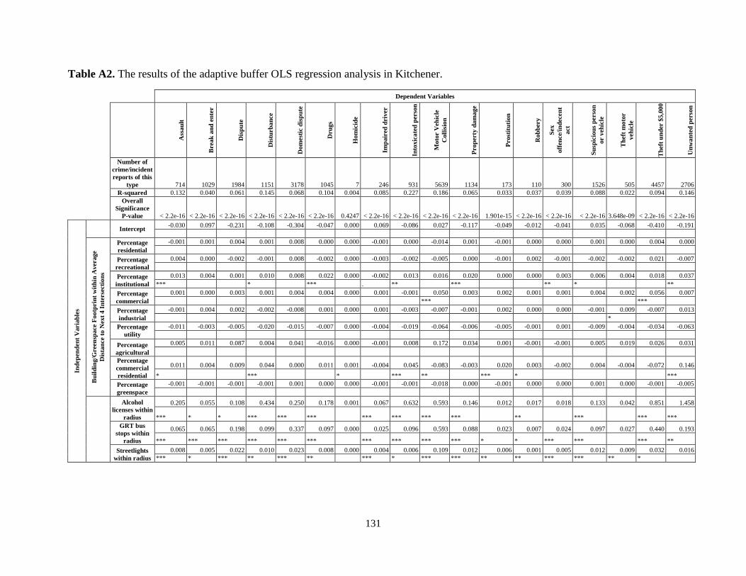
131
Table A2. The results of the adaptive buffer OLS regression analysis in Kitchener.
Dependent Variables
Ass
au
lt
Brea
k a
nd
en
ter
Dis
pu
te
Dis
turb
an
ce
Do
mest
ic d
isp
ute
Dru
gs
Ho
mic
ide
Imp
air
ed
driv
er
Into
xic
ate
d p
erso
n
Mo
tor V
eh
icle
Co
llis
ion
Pro
perty
da
ma
ge
Pro
stit
uti
on
Ro
bb
ery
Sex
off
en
ce/i
nd
ecen
t
act
Su
spic
iou
s p
erso
n
or v
eh
icle
Th
eft
mo
tor
veh
icle
Th
eft
un
der $
5,0
00
Un
wa
nte
d p
erso
n
Number of
crime/incident
reports of this
type 714 1029 1984 1151 3178 1045 7 246 931 5639 1134 173 110 300 1526 505 4457 2706
R-squared 0.132 0.040 0.061 0.145 0.068 0.104 0.004 0.085 0.227 0.186 0.065 0.033 0.037 0.039 0.088 0.022 0.094 0.146
Overall
Significance
P-value < 2.2e-16 < 2.2e-16 < 2.2e-16 < 2.2e-16 < 2.2e-16 < 2.2e-16 0.4247 < 2.2e-16 < 2.2e-16 < 2.2e-16 < 2.2e-16 1.901e-15 < 2.2e-16 < 2.2e-16 < 2.2e-16 3.648e-09 < 2.2e-16 < 2.2e-16
Ind
ep
en
den
t V
aria
ble
s
Intercept -0.030 0.097 -0.231 -0.108 -0.304 -0.047 0.000 0.069 -0.086 0.027 -0.117 -0.049 -0.012 -0.041 0.035 -0.068 -0.410 -0.191
Bu
ild
ing/G
reen
spa
ce F
oo
tprin
t w
ith
in A
vera
ge
Dis
tan
ce t
o N
ex
t 4
In
terse
cti
on
s
Percentage
residential
-0.001 0.001 0.004 0.001 0.008 0.000 0.000 -0.001 0.000 -0.014 0.001 -0.001 0.000 0.000 0.001 0.000 0.004 0.000
Percentage
recreational
0.004 0.000 -0.002 -0.001 0.008 -0.002 0.000 -0.003 -0.002 -0.005 0.000 -0.001 0.002 -0.001 -0.002 -0.002 0.021 -0.007
Percentage
institutional
0.013 0.004 0.001 0.010 0.008 0.022 0.000 -0.002 0.013 0.016 0.020 0.000 0.000 0.003 0.006 0.004 0.018 0.037
*** * *** . ** *** ** * **
Percentage
commercial
0.001 0.000 0.003 0.001 0.004 0.004 0.000 0.001 -0.001 0.050 0.003 0.002 0.001 0.001 0.004 0.002 0.056 0.007
*** ***
Percentage
industrial
-0.001 0.004 0.002 -0.002 -0.008 0.001 0.000 0.001 -0.003 -0.007 -0.001 0.002 0.000 0.000 -0.001 0.009 -0.007 0.013
*
Percentage
utility
-0.011 -0.003 -0.005 -0.020 -0.015 -0.007 0.000 -0.004 -0.019 -0.064 -0.006 -0.005 -0.001 0.001 -0.009 -0.004 -0.034 -0.063
Percentage
agricultural
0.005 0.011 0.087 0.004 0.041 -0.016 0.000 -0.001 0.008 0.172 0.034 0.001 -0.001 -0.001 0.005 0.019 0.026 0.031
Percentage
commercial
residential
0.011 0.004 0.009 0.044 0.000 0.011 0.001 -0.004 0.045 -0.083 -0.003 0.020 0.003 -0.002 0.004 -0.004 -0.072 0.146
* *** * *** ** *** * ***
Percentage
greenspace
-0.001 -0.001 -0.001 -0.001 0.001 0.000 0.000 -0.001 -0.001 -0.018 0.000 -0.001 0.000 0.000 0.001 0.000 -0.001 -0.005
Alcohol
licenses within
radius
0.205 0.055 0.108 0.434 0.250 0.178 0.001 0.067 0.632 0.593 0.146 0.012 0.017 0.018 0.133 0.042 0.851 1.458
*** * * *** *** *** *** *** *** *** ** *** *** ***
GRT bus
stops within
radius
0.065 0.065 0.198 0.099 0.337 0.097 0.000 0.025 0.096 0.593 0.088 0.023 0.007 0.024 0.097 0.027 0.440 0.193
*** *** *** *** *** *** *** *** *** *** * * *** *** *** **
Streetlights
within radius
0.008 0.005 0.022 0.010 0.023 0.008 0.000 0.004 0.006 0.109 0.012 0.006 0.001 0.005 0.012 0.009 0.032 0.016
*** * *** ** *** ** *** * *** *** ** ** *** *** ** *

132
Table A3. The results of the 90 m buffer logistic regression analysis in Kitchener.
Dependent Variables
A
ssa
ult
Brea
k a
nd
en
ter
Dis
pu
te
Dis
turb
an
ce
Do
mest
ic d
isp
ute
Dru
gs
Ho
mic
ide
Imp
air
ed
driv
er
Into
xic
ate
d
perso
n
MV
C
Pro
perty
da
ma
ge
Pro
stit
uti
on
Ro
bb
ery
Sex
off
en
ce/i
nd
ecen
t
act
Su
spic
iou
s p
erso
n
or v
eh
icle
Th
eft
mo
tor
veh
icle
Th
eft
un
der
$5,0
00
Un
wa
nte
d p
erso
n
Number of
intersections
with
crime/incident
report type
present 370 682 753 511 1049 470 7 175 398 1245 628 62 90 219 928 296 1240 641
Chi-Square 160.976 57.143 97.427 239.570 109.534 219.945 13.495 130.906 352.242 347.164 129.637 94.650 69.830 63.661 75.375 91.160 120.913 314.478
Chi-Square P-
value 0.000 0.000 0.000 0.000 0.000 0.000 0.334 0.000 0.000 0.000 0.000 0.000 0.000 0.000 0.000 0.000 0.000 0.000
Ind
ep
en
den
t V
aria
ble
s
Intercept -3.895 -2.152 -16.662 -16.914 -3.943 -2.415 -25.140 -2.300 -17.250 -1.061 -3.695 -19.279 -17.869 -16.641 -2.141 -3.087 -3.165 -2.882
*** *** *** *** *** ** *** *** *** *** ***
Bu
ild
ing/G
reen
space F
oo
tprin
t w
ith
in 9
0m
Percentage
residential
0.012 0.010 0.155 0.147 0.032 0.001 0.185 -0.017 0.140 -0.002 0.022 0.138 0.136 0.137 0.010 0.004 0.025 0.008
** *** * * ***
Percentage
recreational
0.012 -0.016 0.156 0.146 0.034 0.004 -44.230 -0.020 0.143 0.022 0.014 0.121 0.162 0.128 0.003 0.004 0.041 0.021
* ***
Percentage
institutional
0.034 0.020 0.151 0.162 0.030 0.016 0.184 -0.013 0.159 0.016 0.037 0.168 0.139 0.157 0.024 0.016 0.034 0.029
** ** ** * ** *** *** *** ***
Percentage
commercial
0.025 0.009 0.157 0.156 0.029 0.010 0.187 0.007 0.157 0.012 0.028 0.162 0.157 0.148 0.014 0.016 0.029 0.023
* ** ** ** ** * *** ***
Percentage
industrial
0.019 0.018 0.160 0.150 0.023 0.008 0.203 0.002 0.143 0.012 0.030 0.156 0.134 0.143 0.012 0.020 0.029 0.016
. ** * ** ** * * *** *
Percentage
utility
-0.083 0.011 0.183 0.089 0.031 0.009 -17.020 -0.026 0.143 -0.038 -0.011 -0.112 0.130 0.170 -0.030 0.011 0.004 -0.023
Percentage
agricultural
-1.648 -1.823 -1.898 0.233 -1.937 -1.734 -2.664 -1.668 0.240 2.031 -1.803 -1.614 -1.602 -1.622 -1.881 -1.643 -1.959 -1.778
Percentage
commercial
residential
0.029 0.004 0.166 0.175 0.035 0.022 0.242 -0.012 0.167 0.022 0.031 0.179 0.166 0.137 0.019 -0.013 0.023 0.028
* *
Percentage
greenspace
0.016 0.006 0.148 0.141 0.025 0.001 -203.000 -0.007 0.145 -0.001 0.018 0.138 0.133 0.136 0.010 0.000 0.021 0.005
* * **
Alcohol licenses
within 90m
0.069 0.197 -0.016 0.074 0.085 0.265 -0.348 -0.121 0.073 -0.095 0.088 -0.196 -0.141 0.009 -0.045 0.073 0.102 0.156
** ** .
GRT bus stops
within 90m
0.151 0.096 0.183 0.231 0.103 0.209 -0.052 0.178 0.313 0.346 0.202 0.086 0.098 0.126 0.113 0.116 0.099 0.162
*** * *** *** ** *** *** *** *** *** ** ** ** ** ***
Streetlights
within 90m
0.027 -0.012 0.010 0.039 0.034 0.023 0.093 0.042 0.069 0.055 -0.004 0.075 0.040 0.006 0.024 0.017 0.028 0.043
* ** *** ** *** *** ** * ** ***

133
Table A4. The results of the adaptive buffer logistic regression analysis in Kitchener.
Dependent Variables
Ass
au
lt
Brea
k a
nd
En
ter
Dis
pu
te
Dis
turb
an
ce
Do
mest
ic d
isp
ute
Dru
gs
Ho
mic
ide
Imp
air
ed
driv
er
Into
xic
ate
d
perso
n
MV
C
Pro
perty
da
ma
ge
Pro
stit
uti
on
Ro
bb
ery
Sex
off
en
ce/i
nd
ecen
t
act
Su
spic
iou
s p
erso
n
or v
eh
icle
Th
eft
mo
tor
veh
icle
Th
eft
un
der
$5,0
00
Un
wa
nte
d p
erso
n
Number of
intersections
with
crime/incident
report type
present 370 682 753 511 1049 470 7 175 398 1245 628 62 90 219 928 296 1240 641
Chi-Square 226.978 93.187 200.446 314.197 211.213 297.521 6.944 168.609 401.187 421.149 193.186 107.024 79.930 98.444 161.742 152.748 245.486 380.674
Chi-Square P-
value 0.000 0.000 0.000 0.000 0.000 0.000 0.861 0.000 0.000 0.000 0.000 0.000 0.000 0.000 0.000 0.000 0.000 0.000
Ind
ep
en
den
t V
aria
ble
s
Intercept
-3.269 -3.060 -15.963 -15.961 -14.917 -3.234 -26.810 -2.508 -16.016 -1.427 -15.846 -26.840 -27.010 -15.883 -1.957 -15.879 -14.917 -15.891
** ** ** *** **
Bu
ild
ing/G
reen
space F
oo
tprin
t w
ith
in A
vera
ge
Dis
tan
ce t
o N
ext
4 I
nte
rse
cti
on
s
Percentage
residential
0.001 0.015 0.142 0.134 0.137 0.005 0.205 -0.019 0.127 -0.001 0.138 0.214 0.224 0.125 0.005 0.128 0.138 0.135
*
Percentage
recreational
0.009 0.006 0.138 0.144 0.145 0.014 -161.000 -0.033 0.138 0.031 0.139 0.184 0.246 0.102 -0.007 0.132 0.158 0.152
*
Percentage
institutional
0.024 0.024 0.135 0.146 0.134 0.022 0.193 -0.017 0.149 0.018 0.152 0.245 0.224 0.144 0.016 0.135 0.148 0.156
* * * ** *
Percentage
commercial
0.010 0.012 0.140 0.141 0.133 0.012 0.196 0.002 0.138 0.010 0.139 0.235 0.242 0.130 0.005 0.131 0.139 0.149
Percentage
industrial
0.004 0.021 0.143 0.131 0.122 0.010 0.201 -0.001 0.123 0.010 0.142 0.228 0.220 0.121 0.002 0.141 0.136 0.141
*
Percentage
utility
-0.200 -0.021 0.120 0.061 0.094 0.005 -618.900 -0.096 0.122 -0.047 0.090 -0.962 0.179 0.141 -0.040 0.081 0.093 0.098
Percentage
agricultural
0.073 0.026 0.149 0.200 0.095 -3131.000 -2029.000 -1.188 0.222 0.558 0.216 -2453.000 -2808.000 0.104 0.042 0.261 0.086 0.150
Percentage
commercial
residential
0.029 0.019 0.156 0.176 0.149 0.043 0.253 -0.003 0.185 0.032 0.155 0.269 0.256 0.121 0.007 0.120 0.148 0.169
. ** *
Percentage
greenspace
0.001 0.011 0.133 0.126 0.129 0.002 0.181 -0.012 0.126 -0.002 0.133 0.205 0.218 0.121 0.004 0.122 0.132 0.131
Alcohol licenses
within 90m
0.170 0.164 0.046 0.255 0.188 0.308 0.199 0.102 0.344 0.170 0.180 0.063 0.049 0.084 0.164 0.221 0.202 0.294
** ** *** ** *** *** * ** ** ** ** ***
GRT bus stops
within 90m
0.211 0.124 0.220 0.256 0.157 0.203 -0.129 0.180 0.292 0.275 0.192 0.169 0.145 0.177 0.164 0.146 0.126 0.194
*** *** *** *** *** *** *** *** *** *** ** ** *** *** *** *** ***
Streetlights
within 90m
0.032 0.014 0.036 0.030 0.038 0.028 0.043 0.035 0.032 0.036 0.024 0.034 0.036 0.029 0.027 0.032 0.042 0.029
*** ** *** *** *** *** *** *** *** *** ** *** *** *** *** *** ***

134
Table A5. The results of the AKDE OLS regression analysis in Kitchener-Waterloo.
Dependent Variables
Ass
au
lt
Brea
k a
nd
en
ter
Dis
pu
te
Dis
turb
an
ce
Do
mest
ic d
isp
ute
Dru
gs
Ho
mic
ide
Imp
air
ed
driv
er
Into
xic
ate
d p
erso
n
MV
C
Pro
perty
da
ma
ge
Pro
stit
uti
on
Ro
bb
ery
Sex
off
en
ce i
nd
ecen
t
act
Su
spic
iou
s p
erso
n o
r
veh
icle
Th
eft
mo
tor v
eh
icle
Th
eft
un
der $
5,0
00
do
lla
rs
Un
wa
nte
d p
erso
n
Number of
crime/incident
reports of this type 982 1512 2480 1678 3865 1435 9 383 1351 8389 1818 175 144 415 2172 642 6884 3559
R-squared 0.084 0.014 0.025 0.128 0.034 0.068 0.007 0.030 0.123 0.058 0.057 0.022 0.023 0.015 0.030 0.022 0.028 0.113
Overall p-value 2.39E-10 2.39E-10 < 2.2E-16 < 2.2E-16 < 2.2E-16 < 2.2E-16 0.00024 < 2.2E-16 < 2.2E-16 < 2.2E-16 < 2.2E-16 < 2.2E-16 < 2.2E-16 2.97E-11 < 2.2E-16 < 2.2E-16 < 2.2E-16 < 2.2e-16
Intercept
0.034 0.243 0.319 0.108 0.440 0.048 0.002 0.054 0.008 0.947 0.195 -0.009 0.009 0.045 0.271 0.099 0.582 -0.027
*** *** ** *** *** *** *** *** *** *** **
Ind
ep
en
den
t V
aria
ble
s
AKDE values
Elementary schools
0.016 0.005 0.005 0.010 0.040 -0.004 -0.001 -0.002 -0.003 -0.124 0.008 -0.009 -0.002 0.002 0.020 -0.008 -0.054 0.008
*
AKDE values GRT
bus stops
0.005 0.004 0.012 0.005 0.022 0.011 0.000 0.001 0.009 0.052 0.007 0.001 0.001 0.002 0.010 0.002 0.050 0.023
*** *** *** ** *** *** *** *** * *** *** *** *** ***
AKDE values
Hospitals
0.056 0.005 -0.040 0.013 -0.086 0.069 -0.001 -0.009 0.084 -0.030 -0.005 -0.007 -0.006 0.005 -0.052 0.009 -0.061 0.121
AKDE values LCBO
and Beer Stores
0.002 0.016 0.027 -0.060 0.006 0.001 0.000 0.048 0.044 0.797 0.002 -0.019 0.010 -0.008 0.052 0.006 0.829 0.198
*** *** * *** *
AKDE values
Libraries,
community centres,
and arenas
0.022 -0.011 0.063 0.005 0.083 -0.025 0.001 0.006 -0.047 0.066 0.051 -0.020 -0.005 0.009 0.009 0.016 0.135 -0.147
*
*
*
AKDE values
Licensed restaurants
0.012 0.001 -0.001 0.030 -0.006 0.007 0.000 0.003 0.027 0.017 0.010 0.000 0.001 -0.001 0.000 0.002 0.022 0.057
*** *** * *** *** *** ** *** ** * ***
AKDE values Places
of worship
0.005 0.004 0.011 0.009 0.011 0.005 0.001 0.001 0.004 -0.048 -0.002 0.020 0.000 0.002 0.017 -0.003 -0.059 0.073
*** * *** ** ***
AKDE values
Secondary schools
0.098 0.009 0.006 0.206 0.118 0.438 -0.002 -0.010 0.015 0.334 0.046 0.019 0.026 0.037 -0.021 -0.020 0.354 0.271
*** *** * *** * *** *** *
AKDE values
Universities
-0.023 0.113 0.098 0.282 0.060 0.005 -0.002 -0.049 0.286 -0.031 -0.004 -0.045 -0.023 -0.006 0.047 0.027 0.121 0.390
** *** ** *** ** *
AKDE values WRPS
police stations
0.281 0.080 0.079 0.064 0.197 0.366 -0.001 0.001 0.193 0.561 1.217 0.017 -0.005 0.001 0.003 0.358 0.235 0.092
*** * * *** ** ** *** ***

135
Table A6. The results of the AKDE logistic regression analysis in Kitchener-Waterloo.
Dependent Variables
Ass
au
lt
Brea
k a
nd
en
ter
Dis
pu
te
Dis
turb
an
ce
Do
mest
ic d
isp
ute
Dru
gs
Ho
mic
ide
Imp
air
ed
driv
er
Into
xic
ate
d p
erso
n
MV
C
Pro
perty
da
ma
ge
Pro
stit
uti
on
Ro
bb
ery
Sex
off
en
ce i
nd
ecen
t
act
Su
spic
iou
s p
erso
n o
r
veh
icle
Th
eft
mo
tor v
eh
icle
Th
eft
un
der $
5,0
00
do
lla
rs
Un
wa
nte
d p
erso
n
Number of
intersections with
crime/incident report
type present 491 941 1003 711 1402 615 9 264 553 1819 898 64 117 302 1293 387 1816 879
Chi-squared 201.291 87.309 118.739 336.597 158.078 284.098 20.185 83.962 422.680 276.630 156.624 132.455 57.785 68.715 137.801 73.579 221.969 413.065
Chi-squared
Significant 0.000 0.000 0.000 0.000 0.000 0.000 0.028 0.000 0.000 0.000 0.000 0.000 0.000 0.000 0.000 0.000 0.000 0.000
Wald Chi-squared 1958.305 1353.782 1252.547 1710.630 639.126 1836.767 348.116 1934.623 1904.837 183.125 1423.527 1140.635 1507.475 1973.793 794.704 2001.764 185.486 1454.101
Wald Chi-squared
Significant 0.000 0.000 0.000 0.000 0.000 0.000 0.000 0.000 0.000 0.000 0.000 0.000 0.000 0.000 0.000 0.000 0.000 0.000
Intercept
-2.714 -1.637 -1.634 -2.331 -1.195 -2.499 -6.086 -3.065 -2.792 -0.870 -1.804 -5.204 -4.074 -3.071 -1.282 -2.670 -0.792 -2.087
*** *** *** *** *** *** *** *** *** *** *** *** *** *** *** *** *** ***
Ind
ep
en
den
t V
aria
ble
s
AKDE values
Elementary schools
0.122 0.027 0.024 0.042 0.058 0.047 -6093.000 -0.043 0.031 0.024 0.077 0.066 -0.053 0.039 0.067 -0.009 0.068 0.049
*** ** *** ** *** *
AKDE values GRT
bus stops
0.016 0.011 0.016 0.022 0.014 0.021 -0.012 0.009 0.026 0.019 0.013 0.011 0.015 0.016 0.012 0.012 0.009 0.020
*** *** *** *** *** *** ** *** *** *** * *** *** *** *** *** ***
AKDE values
Hospitals
0.017 0.056 -0.014 -0.017 -0.134 0.152 -26180.000 -0.341 0.059 0.005 0.033 0.230 -0.159 0.018 -0.049 0.012 0.044 0.026
*
AKDE values LCBO
and Beer Stores
0.105 0.050 0.030 0.088 0.051 0.084 0.056 0.206 0.135 0.073 0.077 -0.166 0.127 0.020 0.077 0.111 0.103 0.134
* *** ** * * **
AKDE values
Libraries, community
centres, and arenas
0.095 0.003 0.057 0.035 0.040 0.042 0.280 0.008 0.055 0.071 0.022 -0.159 0.009 0.092 0.041 0.036 0.079 0.043
* *
AKDE values
Licensed restaurants
0.007 -0.001 0.000 0.009 -0.001 0.008 -0.002 0.010 0.011 0.014 0.006 0.004 0.005 -0.004 -0.003 0.005 0.012 0.013
** *** ** *** *** *** * *** ***
AKDE values Places
of worship
0.034 0.033 0.023 0.037 0.039 0.036 0.120 0.012 0.048 0.025 0.018 0.124 0.020 0.026 0.044 0.006 0.048 0.057
*** *** ** *** *** *** *** *** ** * *** * *** *** ***
AKDE values
Secondary schools
0.160 0.083 0.073 0.232 0.171 0.218 -6396.000 -0.035 0.128 0.157 0.192 0.207 0.319 0.229 0.027 -0.067 0.142 0.132
* *** ** *** ** *** *** ** * *
AKDE values
Universities
-0.099 -0.069 -0.059 0.218214 0.029 -0.036 -3490.000 -0.228 0.218 0.051 0.091 -0.321 -0.380 -0.041 0.064 0.082 -0.077 0.304
*
AKDE values WRPS
police stations
0.086 0.206 0.084 0.144 0.000 0.060 -748.800 0.012 0.127 0.151 0.185 0.352 -0.222 -0.069 0.130 0.199 0.049 0.216
* * * * *