An Observational Estimate of Inferred Ocean Energy Divergence

An Observational Estimate of Inferred Ocean Energy Divergence

KEVIN E. TRENBERTH AND JOHN T. FASULLO

National Center for Atmospheric Research,* Boulder, Colorado

(Manuscript received 2 May 2007, in final form 25 September 2007)

ABSTRACT

Monthly net surface energy fluxes (FS) over the oceans are computed as residuals of the atmosphericenergy budget using top-of-atmosphere (TOA) net radiation (RT) and the complete atmospheric energy(AE) budget tendency (�AE/�t) and divergence (� · FA). The focus is on TOA radiation from the EarthRadiation Budget Experiment (ERBE) (February 1985–April 1989) and the Clouds and Earth’s RadiantEnergy System (CERES) (March 2000–May 2004) satellite observations combined with results from twoatmospheric reanalyses and three ocean datasets that enable a comprehensive estimate of uncertainties.Surface energy flux departures from the annual mean and the implied annual cycle in “equivalent oceanenergy content” are compared with the directly observed ocean energy content (OE) and tendency (�OE/�t)to reveal the inferred annual cycle of divergence (� · FO). In the extratropics, the surface flux dominates theocean energy tendency, although it is supplemented by ocean Ekman transports that enhance the annualcycle in ocean heat content. In contrast, in the tropics, ocean dynamics dominate OE variations throughoutthe year in association with the annual cycle in surface wind stress and the North Equatorial Current. Ananalysis of the regional characteristics of the first joint empirical orthogonal function (EOF) of FS, �OE/�t,and � · FO is presented, and the largest sources of uncertainty are attributed to variations in OE. The meanand annual cycle of zonal mean global ocean meridional heat transports are estimated. The annual cyclereveals the strongest poleward heat transports in each hemisphere in the cold season, from November toApril in the north and from May to October in the south, with a substantial across-equatorial transport,exceeding 4 PW in some months. Annual mean results do not differ greatly from some earlier estimates, butthe sources of uncertainty are exposed. Comparison of annual means with direct ocean observations givesreasonable agreement, except in the North Atlantic, where transports from the ocean transects are slightlygreater than the estimates presented here.

1. Introduction

The oceans play a major role in moderating climate.In midlatitudes, energy absorbed by the oceans in sum-mer is released to the atmosphere in winter, thus re-ducing the annual cycle in surface temperatures relativeto those over land. Moreover, the advection of energyfrom the oceans also moderates the seasonal cycle overland where maritime influences prevail. Relative to theoceans, the atmosphere’s capacity to store energy issmall and equivalent to that of about 3.5 m of the ocean

if their associated proportion of global coverage is con-sidered. Because the main movement of energy in theland and ice components is by conduction, only verylimited masses are involved in changes on annual timescales. Moreover, water has a much higher specific heatthan dry land by about a factor of 4.5 or so. Accord-ingly, it is the oceans, through their total mass, heatcapacity, and movement of energy by turbulence, con-vection, and advection, that have an enormous impacton the global energy budget, which can vary signifi-cantly on annual and longer time scales (Trenberth andStepaniak 2004).

The net radiative flux (RT) at the top of the atmo-sphere (TOA) on longer-than-annual time scales ismostly balanced by transports of energy by the atmo-sphere and ocean, and local upward surface energyfluxes (FS) are largely offset by the ocean’s divergentenergy transport (� · FO) (Trenberth and Caron 2001).In contrast, for the annual cycle in midlatitudes the

* The National Center for Atmospheric Research is sponsoredby the National Science Foundation.

Corresponding author address: Kevin E. Trenberth, NationalCenter for Atmospheric Research, P.O. Box 3000, Boulder, CO80307-3000.E-mail: [email protected]

984 J O U R N A L O F P H Y S I C A L O C E A N O G R A P H Y VOLUME 38

DOI: 10.1175/2007JPO3833.1

© 2008 American Meteorological Society

JPO3833

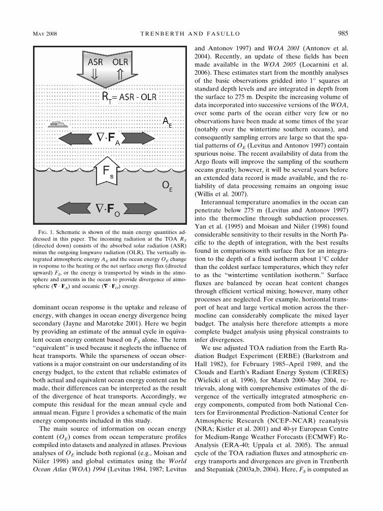
dominant ocean response is the uptake and release ofenergy, with changes in ocean energy divergence beingsecondary (Jayne and Marotzke 2001). Here we beginby providing an estimate of the annual cycle in equiva-lent ocean energy content based on FS alone. The term“equivalent” is used because it neglects the influence ofheat transports. While the sparseness of ocean obser-vations is a major constraint on our understanding of itsenergy budget, to the extent that reliable estimates ofboth actual and equivalent ocean energy content can bemade, their differences can be interpreted as the resultof the divergence of heat transports. Accordingly, wecompute this residual for the mean annual cycle andannual mean. Figure 1 provides a schematic of the mainenergy components included in this study.

The main source of information on ocean energycontent (OE) comes from ocean temperature profilescompiled into datasets and analyzed in atlases. Previousanalyses of OE include both regional (e.g., Moisan andNiiler 1998) and global estimates using the WorldOcean Atlas (WOA) 1994 (Levitus 1984, 1987; Levitus

and Antonov 1997) and WOA 2001 (Antonov et al.2004). Recently, an update of these fields has beenmade available in the WOA 2005 (Locarnini et al.2006). These estimates start from the monthly analysesof the basic observations gridded into 1° squares atstandard depth levels and are integrated in depth fromthe surface to 275 m. Despite the increasing volume ofdata incorporated into successive versions of the WOA,over some parts of the ocean either very few or noobservations have been made at some times of the year(notably over the wintertime southern oceans), andconsequently sampling errors are large so that the spa-tial patterns of OE (Levitus and Antonov 1997) containspurious noise. The recent availability of data from theArgo floats will improve the sampling of the southernoceans greatly; however, it will be several years beforean extended data record is made available, and the re-liability of data processing remains an ongoing issue(Willis et al. 2007).

Interannual temperature anomalies in the ocean canpenetrate below 275 m (Levitus and Antonov 1997)into the thermocline through subduction processes.Yan et al. (1995) and Moisan and Niiler (1998) foundconsiderable sensitivity to their results in the North Pa-cific to the depth of integration, with the best resultsfound in comparisons with surface flux for an integra-tion to the depth of a fixed isotherm about 1°C colderthan the coldest surface temperatures, which they referto as the “wintertime ventilation isotherm.” Surfacefluxes are balanced by ocean heat content changesthrough efficient vertical mixing; however, many otherprocesses are neglected. For example, horizontal trans-port of heat and large vertical motion across the ther-mocline can considerably complicate the mixed layerbudget. The analysis here therefore attempts a morecomplete budget analysis using physical constraints toinfer divergences.

We use adjusted TOA radiation from the Earth Ra-diation Budget Experiment (ERBE) (Barkstrom andHall 1982), for February 1985–April 1989, and theClouds and Earth’s Radiant Energy System (CERES)(Wielicki et al. 1996), for March 2000–May 2004, re-trievals, along with comprehensive estimates of the di-vergence of the vertically integrated atmospheric en-ergy components, computed from both National Cen-ters for Environmental Prediction–National Center forAtmospheric Research (NCEP–NCAR) reanalysis(NRA; Kistler et al. 2001) and 40-yr European Centrefor Medium-Range Weather Forecasts (ECMWF) Re-Analysis (ERA-40; Uppala et al. 2005). The annualcycle of the TOA radiation fluxes and atmospheric en-ergy transports and divergences are given in Trenberthand Stepaniak (2003a,b, 2004). Here, FS is computed as

FIG. 1. Schematic is shown of the main energy quantities ad-dressed in this paper. The incoming radiation at the TOA RT

(directed down) consists of the absorbed solar radiation (ASR)minus the outgoing longwave radiation (OLR). The vertically in-tegrated atmospheric energy AE and the ocean energy OE changein response to the heating or the net surface energy flux (directedupward) FS, or the energy is transported by winds in the atmo-sphere and currents in the ocean to provide divergence of atmo-spheric (� · FA) and oceanic (� · FO) energy.

MAY 2008 T R E N B E R T H A N D F A S U L L O 985

a residual that allows the implied annual mean � · FO tobe inferred. The transports derived from this methodhave been shown to correspond quite well with directobservations from ocean hydrographic sections (Tren-berth and Caron 2001).

Here we examine the annual cycle of FS and compareit with direct observations of OE from three sources,including WOA 2005 (Locarnini et al. 2006), the analy-sis of the Japanese Meteorological Association version6.2 (JMA; Ishii et al. 2006), and the Global Ocean DataAssimilation System (GODAS; Behringer and Xue2004; Behringer 2007). We analyze the overall oceanenergy budget and its agreement with fundamentalglobal constraints in a range of estimates. We concludethat many of the results are dominated by physicallyreal changes, thereby revealing new aspects of the an-nual cycle of ocean energy divergence. Nevertheless,residual errors are significant in instances, and theirinfluence is quantified. Section 2 describes the data andthe processing, section 3 presents the results, and sec-tion 4 discusses the results and their implications; con-clusions are drawn in section 5.

2. Data and methods

A more detailed discussion of the datasets and meth-ods is given in Fasullo and Trenberth (2008a, hereafterFT08). We use a prime to denote a departure from theannual mean. Figure 1 illustrates the relationships out-lined in the equations below.

a. Energy budgets

The dominant energy terms and balances for the ver-tically integrated atmosphere and ocean are presentedbriefly below. In the atmosphere,

FS � � · FA � �AE��t � RT, �1�

where FS and RT have been previously defined, and� · FA and �AE/�t are the vertically integrated atmo-spheric total energy divergence and tendency, respec-tively. Moreover, for the ocean, given FS and OE, thedivergence of ocean energy transport can be inferredbased on

� · FO � FS � �OE ��t � 0, �2�

and the ocean energy is approximated by the oceanheat content,

OE � �T�z��Cw dz, �3�

where z is depth, is water density, T is the oceantemperature, and Cw is the specific heat of seawater.The challenges in diagnosing the terms in (1)–(3) in-

clude obtaining high-quality analyses of global obser-vations with adequate sampling of the large temporaland spatial gradients of all terms.

b. Adjusted satellite retrievals

For terms in the TOA budget contributing to RT,adjusted satellite retrievals from ERBE (February1985–April 1989; Barkstrom and Hall 1982; FT08) andCERES (March 2000–May 2004; Wielicki et al. 1996;FT08) are used. While the ERBE retrievals offer multi-satellite sampling, the CERES data show lower noise,improved ties to ground calibration, and smaller fieldsof view than ERBE (Loeb et al. 2007). CERES instru-ment calibration stability on Terra is claimed to be typi-cally better than 0.2%, and calibration consistencyfrom ground to space is better than 0.25%. Becauseboth the ERBE and CERES estimates are known tocontain spurious imbalances, however (Trenberth 1997;Wielicki et al. 2006), adjustments are required, as de-scribed in FT08, such that estimates of the global im-balance during the ERBE and CERES periods(Hansen et al. 2005; Willis et al. 2004; Huang 2006;Levitus et al. 2005) are matched. Associated uncer-tainty estimates, equal to two sample standard devia-tions of interannual variability (2�), are reportedhere to quantify the uncertainty associated with the lim-ited ERBE and CERES time periods. For all analysishere these adjusted ERBE and CERES fields are thusused, and in no instances are the raw fields used.

c. Reanalysis datasets

To solve for FS from (2), estimates of the atmo-spheric tendency and divergence are required, exceptfor the global average where divergence is zero by defi-nition. In constructing estimates of these terms we useonly fields strongly influenced by observations, such assurface pressure and atmospheric temperature and hu-midity from NRA and ERA-40. Estimates of themonthly mean vertically integrated storage, transports,and divergence of energy within the atmosphere forERA-40 and NRA were computed and evaluated as inTrenberth et al. (2001), and for NRA these estimateshave been updated through 2006 (additional informa-tion available online at http://www.cgd.ucar.edu/cas/catalog/newbudgets; see also Trenberth and Stepaniak2003a,b; FT08). However, because ERA-40 fields arenot available beyond 2001, the ERBE period is theprimary focus of the present study.

d. Ocean surface fluxes and storage

The computation of FS as a residual is superior toboth model-based and Comprehensive Ocean Atmo-sphere Dataset (COADS) surface fluxes in terms of


biases, because the latter both suffer from systematicbiases and fail to satisfy global constraints (Trenberthet al. 2001). Grist and Josey (2003) wrestled with how tobest adjust their COADS-based estimates to satisfy en-ergy transport constraints, suggesting adjustments tothe fluxes and the need for further refinements associ-ated with clouds. Trenberth and Caron (2001) used thelong-term annual means of FS during the ERBE periodto compute the implied meridional ocean energy trans-ports. Results agreed quite well with independent esti-mates from direct ocean measurements within the errorbars of each in numerous sections. Moreover, they arereasonably compatible with estimates from state-of-the-art coupled climate models. However, the annualmean FS (Trenberth et al. 2001; Trenberth and Stepa-niak 2004) likely has various problems, especially overthe southern oceans (Trenberth and Caron 2001).

The ocean datasets used to diagnose ocean heat con-tent include the WOA 2005, JMA, and recently cor-rected (6 February 2006) GODAS. While some insightinto the likely biases of OE from these data can begained from their degree of closure with FS (FT08),uncertainty in the observations, and particularly the de-composition of error into its systematic and randomcomponents, has been hampered by a lack of observa-tions, particularly at depth. Here we also use departuresfrom this mean for the ERBE period and thus gain theadvantage of subtracting out most systematic errors orbiases. Estimates of FS over the ocean are based on (2),and their accuracy is of the order of 20 W m�2 over1000-km scales while satisfying closure among FS,� · FA, �AE/�t, and RT (Trenberth et al. 2001). A can-cellation of errors in � · FA occurs over larger scalesbecause divergence is zero globally by definition. Un-certainty in FS is governed mainly by the uncertaintiesin RT and � · FA. By exploiting the constraint that FS

and �OE/�t must balance globally, FT08 identify an ex-cessive annual cycle of OE in JMA and WOA relative tothat which can be explained by either a broad range ofFS estimates or GODAS fields.

In estimating ocean heat from (3), we essentially fol-low the calculations of Antonov et al. (2004). However,therein the density of seawater () was assumed to be1020 kg m�3 and the specific heat (Cw) was assumed tobe 4187 J kg�1 K�1, whereas for the typical salinity ofthe ocean of �35 PSU, is �1025–1028 kg m�3 and Cw

is 3985–3995 J kg�1 K�1 for temperatures from 2° to20°C. The product Cw is more nearly constant thaneither of the two components, but the Antonov et al.value is 4.4% too high, leading to an overestimate ofOE and its annual cycle. Therefore, we have adjustedthese constants and performed our own integration, us-ing ocean temperatures provided at multiple levels in

the WOA, where the depth of each layer is assumed toextend between the midpoints of each level. In the caseof the surface, the layer is assumed to begin at 0 m andat 250 m-depth the layer is assumed to terminate at 275m, half way to the next WOA layer at 300 m. We assignthe density of ocean water at 1026.5 kg m�3 and specificheat at 3990 J kg�1 K�1, although it is their product thatdetermines OE per (3).

Obvious spurious values of ocean heat content southof 20°S are edited out by accepting only the monthlydepartures from the annual mean within two standarddeviations of the zonal ocean mean to take advantageof the lack of land over the southern oceans. Globally,the data are also filtered temporally by retaining thefirst three harmonics of the annual cycle. Oceanic en-ergy tendencies are then computed by reassembling theFourier series and differencing OE between the startand end days of each month. Other small systematicdifferences may arise from methods of compiling thevertical integral and numerical aspects in computing OE

[which are not described by Antonov et al. (2004)];however, tests show that the magnitude of the annualcycle is not significantly affected by these refinements.In general, the patterns of OE derived here are quitesimilar to the actual OE of Antonov et al. (2004) outsideof the tropics, except the latter are �10%–20% larger.One source of discrepancy can be the depth of integra-tion, and Levitus and Antonov (1997) show that depthsbelow 150 m are often somewhat out of phase withnear-surface values. Deser et al. (1999) show how de-cadal changes in the Kuroshio Extension are associatedwith temperature changes exceeding 1°C in the mainthermocline from 300- to 1000-m depth, and that suchchanges can occur in association with subduction andventilation of the thermocline. However, integrating togreater depth brings in regions of fewer data and thusincreases errors and noise, and we therefore limit thedepth of integration to 275 m. This may lead to errorsin the annual cycle, although the phasing with depthaffects whether it amplifies or diminishes the annualcycle. Analysis of fields integrated to 500 m shows re-sults that are fundamentally unchanged from the resultspresented here.

e. Regridding and standard deviations

To provide a consistent delineation of land–seaboundaries among the datasets, all fields are trans-formed to a grid containing 192 evenly spaced longitu-dinal grid points and 96 Gaussian-spaced latitudinalgrid points using bilinear interpolation (i.e., to a T63grid). Spatial integrals are calculated using Gaussianweights over the T63 grid and a common land–sea maskis applied. Total energy is expressed in units of peta-


watts (PW � 1015 W) and monthly mean values areused for all calculations. In quantifying seasonality, theestimated population standard deviation of monthlyvalues is used.

f. Secondary terms

Within the ocean, the formation and melting of seaice can influence OE. An estimate of this effect from thelatent heat of fusion can be obtained from estimates ofthe annual cycle in ice volume from an ice model byKöberle and Gerdes (2003) for the Arctic, driven byNRA atmospheric fields, of about 1.5–3.2 104 km3,which is also broadly consistent with energy budget es-timates of Serreze et al. (2006, 2007). These studies thussuggest a heating amplitude of 0.5 PW for the annualcycle’s first harmonic. Moreover, the transport of watervapor to land and its storage as either snow or wateraffects the mass of the ocean and sea level (Minster etal.1999) and is associated with an energy flux estimatednear 0.1 PW (FT08). For global budgets, it is expectedthat some degree of compensation between sea ice for-mation in the Antarctic balances that in the Arctic;however, reliable estimates of the net global budgetremain unavailable. Nevertheless, this initial scale com-parison suggests that overall the global imbalance atTOA should be reflected primarily in OE (Levitus et al.2005).

3. Results

a. The annual mean FS

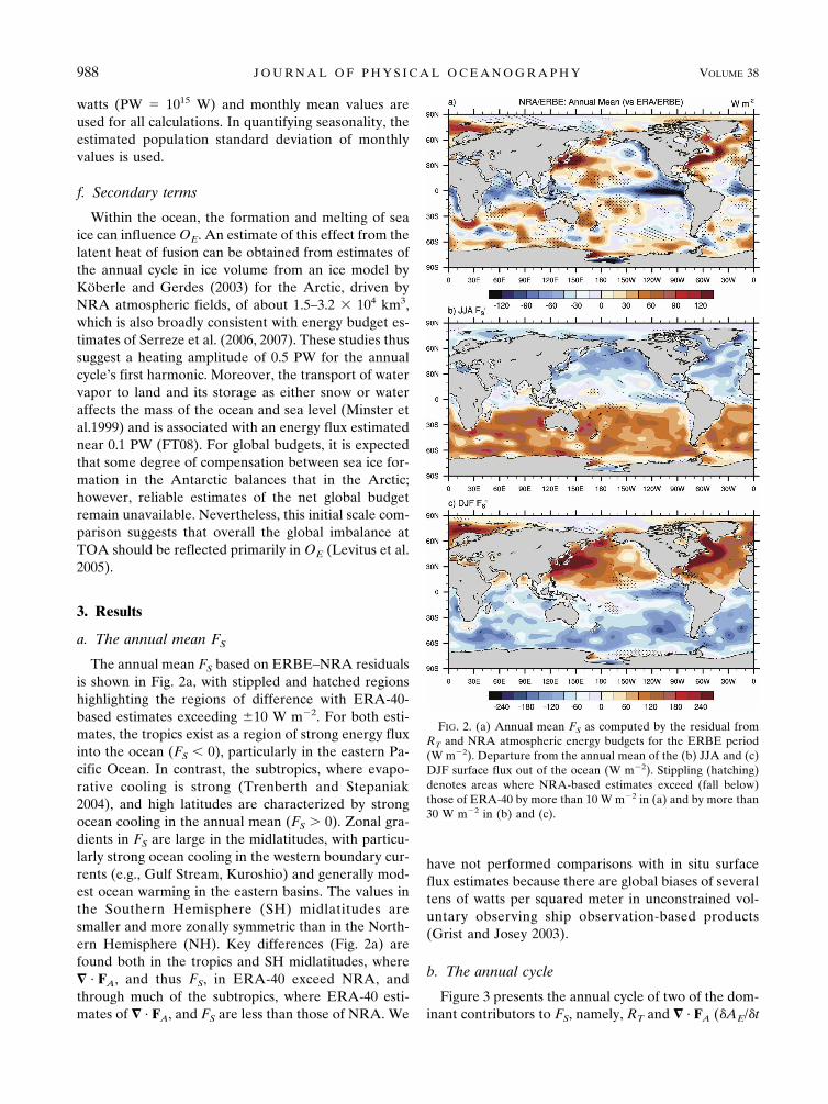
The annual mean FS based on ERBE–NRA residualsis shown in Fig. 2a, with stippled and hatched regionshighlighting the regions of difference with ERA-40-based estimates exceeding 10 W m�2. For both esti-mates, the tropics exist as a region of strong energy fluxinto the ocean (FS � 0), particularly in the eastern Pa-cific Ocean. In contrast, the subtropics, where evapo-rative cooling is strong (Trenberth and Stepaniak2004), and high latitudes are characterized by strongocean cooling in the annual mean (FS � 0). Zonal gra-dients in FS are large in the midlatitudes, with particu-larly strong ocean cooling in the western boundary cur-rents (e.g., Gulf Stream, Kuroshio) and generally mod-est ocean warming in the eastern basins. The values inthe Southern Hemisphere (SH) midlatitudes aresmaller and more zonally symmetric than in the North-ern Hemisphere (NH). Key differences (Fig. 2a) arefound both in the tropics and SH midlatitudes, where� · FA, and thus FS, in ERA-40 exceed NRA, andthrough much of the subtropics, where ERA-40 esti-mates of � · FA, and FS are less than those of NRA. We

have not performed comparisons with in situ surfaceflux estimates because there are global biases of severaltens of watts per squared meter in unconstrained vol-untary observing ship observation-based products(Grist and Josey 2003).

b. The annual cycle

Figure 3 presents the annual cycle of two of the dom-inant contributors to FS, namely, RT and � · FA (�AE/�t

FIG. 2. (a) Annual mean FS as computed by the residual fromRT and NRA atmospheric energy budgets for the ERBE period(W m�2). Departure from the annual mean of the (b) JJA and (c)DJF surface flux out of the ocean (W m�2). Stippling (hatching)denotes areas where NRA-based estimates exceed (fall below)those of ERA-40 by more than 10 W m�2 in (a) and by more than30 W m�2 in (b) and (c).


Fig 2 live 4/C

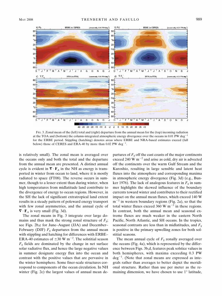
is relatively small). The zonal mean is averaged overthe oceans only and both the total and the departurefrom the annual mean are presented. A distinct annualcycle is evident in � · FA in the NH as energy is trans-ported in winter from ocean to land, where it is mostlyradiated to space (FT08). The reverse occurs in sum-mer, though to a lesser extent than during winter, whenhigh temperatures from midlatitude land contribute tothe divergence of energy to ocean regions. However, inthe SH the lack of significant extratropical land extentresults in a steady pattern of poleward energy transportwith few zonal asymmetries, and the annual cycle of� · FA is very small (Fig. 3d).

The zonal means in Fig. 3 integrate over large do-mains and thus mask the strong zonal structure of FS;see Figs. 2b,c for June–August (JJA) and December–February (DJF) FS departures from the annual meanwith stippling and hatching for differences with ERBE–ERA-40 estimates of 30 W m�2. The solstitial seasonFS fields are dominated by the change in net surfacesolar radiative flux, and hence the large negative valuesin summer designate energy flux into the ocean andcontrast with the positive values that are pervasive inthe winter hemisphere. Some finer-scale structures cor-respond to components of the ocean circulation. In NHwinter (Fig. 2c) the largest values of annual mean de-

partures of FS off the east coasts of the major continentsexceed 240 W m�2 and arise as cold, dry air is advectedoff the continents over the warm Gulf Stream and theKuroshio, resulting in large sensible and latent heatfluxes into the atmosphere and corresponding maximain atmospheric energy divergence (Fig. 3d) (e.g., Bun-ker 1976). The lack of analogous features in FS in sum-mer highlights the skewed influence of the boundarycurrents toward winter and contributes to their rectifiedimpact on the annual mean fluxes, which exceed 140 Wm�2 in western boundary regions (Fig. 2a), so that thetotal winter fluxes exceed 360 W m�2 in these regions.In contrast, both the annual mean and seasonal ex-treme fluxes are much weaker in the eastern NorthPacific, North Atlantic, and SH oceans. In the tropics,seasonal contrasts are less than in midlatitudes, and FS

is positive in the primary upwelling zones for both sol-stitial seasons.

The mean annual cycle of FS zonally averaged overthe oceans (Fig. 4a), which is represented by the differ-ence between Figs. 3b,d, features peak solstice values inboth hemispheres, with maxima exceeding 0.3 PWdeg�1. (Note that zonal means are expressed as inte-grals rather than averages to better depict the meridi-onal structure. Rather than use per meter as the re-maining dimension, we have chosen to use 1° latitude,

FIG. 3. Zonal mean of the (left) total and (right) departure from the annual mean for the (top) incoming radiationat the TOA and (bottom) the column-integrated atmospheric energy divergence over the oceans in 0.01 PW deg�1

for the ERBE period. Stippling (hatching) denotes areas where ERBE and NRA-based estimates exceed (fallbelow) those of CERES and ERA-40 by more than 0.02 PW deg�1.


Fig 3 live 4/C

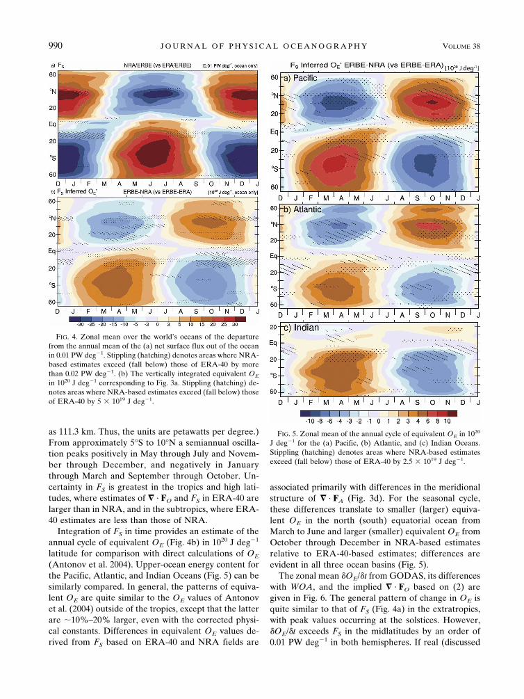
as 111.3 km. Thus, the units are petawatts per degree.)From approximately 5°S to 10°N a semiannual oscilla-tion peaks positively in May through July and Novem-ber through December, and negatively in Januarythrough March and September through October. Un-certainty in FS is greatest in the tropics and high lati-tudes, where estimates of � · FO and FS in ERA-40 arelarger than in NRA, and in the subtropics, where ERA-40 estimates are less than those of NRA.

Integration of FS in time provides an estimate of theannual cycle of equivalent OE (Fig. 4b) in 1020 J deg�1

latitude for comparison with direct calculations of OE

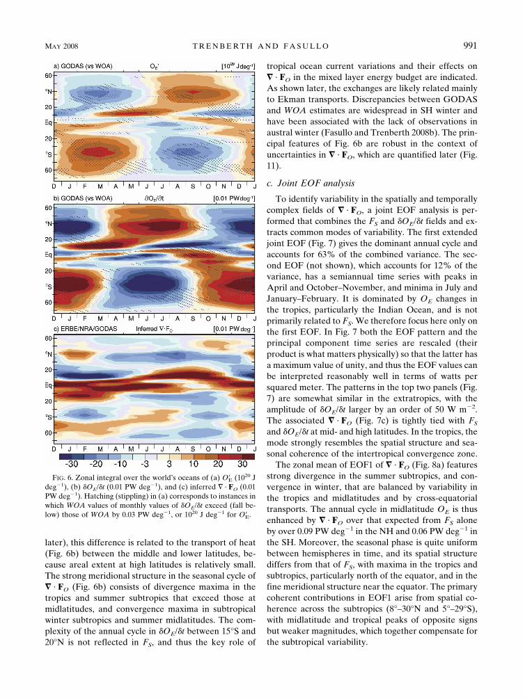
(Antonov et al. 2004). Upper-ocean energy content forthe Pacific, Atlantic, and Indian Oceans (Fig. 5) can besimilarly compared. In general, the patterns of equiva-lent OE are quite similar to the OE values of Antonovet al. (2004) outside of the tropics, except that the latterare �10%–20% larger, even with the corrected physi-cal constants. Differences in equivalent OE values de-rived from FS based on ERA-40 and NRA fields are

associated primarily with differences in the meridionalstructure of � · FA (Fig. 3d). For the seasonal cycle,these differences translate to smaller (larger) equiva-lent OE in the north (south) equatorial ocean fromMarch to June and larger (smaller) equivalent OE fromOctober through December in NRA-based estimatesrelative to ERA-40-based estimates; differences areevident in all three ocean basins (Fig. 5).

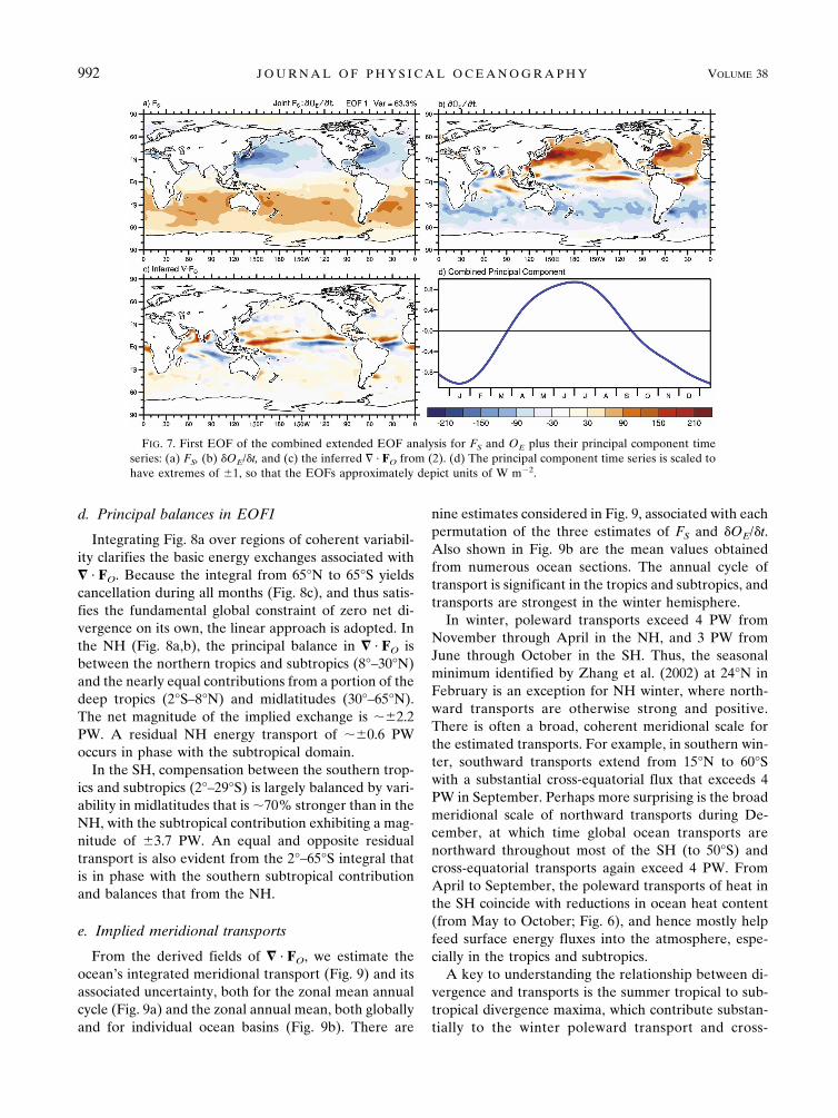
The zonal mean �OE/�t from GODAS, its differenceswith WOA, and the implied � · FO based on (2) aregiven in Fig. 6. The general pattern of change in OE isquite similar to that of FS (Fig. 4a) in the extratropics,with peak values occurring at the solstices. However,�OE/�t exceeds FS in the midlatitudes by an order of0.01 PW deg�1 in both hemispheres. If real (discussed

FIG. 4. Zonal mean over the world’s oceans of the departurefrom the annual mean of the (a) net surface flux out of the oceanin 0.01 PW deg�1. Stippling (hatching) denotes areas where NRA-based estimates exceed (fall below) those of ERA-40 by morethan 0.02 PW deg�1. (b) The vertically integrated equivalent OE

in 1020 J deg�1 corresponding to Fig. 3a. Stippling (hatching) de-notes areas where NRA-based estimates exceed (fall below) thoseof ERA-40 by 5 1019 J deg�1.

FIG. 5. Zonal mean of the annual cycle of equivalent OE in 1020

J deg�1 for the (a) Pacific, (b) Atlantic, and (c) Indian Oceans.Stippling (hatching) denotes areas where NRA-based estimatesexceed (fall below) those of ERA-40 by 2.5 1019 J deg�1.


Fig 4 5 live 4/C

later), this difference is related to the transport of heat(Fig. 6b) between the middle and lower latitudes, be-cause areal extent at high latitudes is relatively small.The strong meridional structure in the seasonal cycle of� · FO (Fig. 6b) consists of divergence maxima in thetropics and summer subtropics that exceed those atmidlatitudes, and convergence maxima in subtropicalwinter subtropics and summer midlatitudes. The com-plexity of the annual cycle in �OE/�t between 15°S and20°N is not reflected in FS, and thus the key role of

tropical ocean current variations and their effects on� · FO in the mixed layer energy budget are indicated.As shown later, the exchanges are likely related mainlyto Ekman transports. Discrepancies between GODASand WOA estimates are widespread in SH winter andhave been associated with the lack of observations inaustral winter (Fasullo and Trenberth 2008b). The prin-cipal features of Fig. 6b are robust in the context ofuncertainties in � · FO, which are quantified later (Fig.11).

c. Joint EOF analysis

To identify variability in the spatially and temporallycomplex fields of � · FO, a joint EOF analysis is per-formed that combines the FS and �OE/�t fields and ex-tracts common modes of variability. The first extendedjoint EOF (Fig. 7) gives the dominant annual cycle andaccounts for 63% of the combined variance. The sec-ond EOF (not shown), which accounts for 12% of thevariance, has a semiannual time series with peaks inApril and October–November, and minima in July andJanuary–February. It is dominated by OE changes inthe tropics, particularly the Indian Ocean, and is notprimarily related to FS. We therefore focus here only onthe first EOF. In Fig. 7 both the EOF pattern and theprincipal component time series are rescaled (theirproduct is what matters physically) so that the latter hasa maximum value of unity, and thus the EOF values canbe interpreted reasonably well in terms of watts persquared meter. The patterns in the top two panels (Fig.7) are somewhat similar in the extratropics, with theamplitude of �OE/�t larger by an order of 50 W m�2.The associated � · FO (Fig. 7c) is tightly tied with FS

and �OE/�t at mid- and high latitudes. In the tropics, themode strongly resembles the spatial structure and sea-sonal coherence of the intertropical convergence zone.

The zonal mean of EOF1 of � · FO (Fig. 8a) featuresstrong divergence in the summer subtropics, and con-vergence in winter, that are balanced by variability inthe tropics and midlatitudes and by cross-equatorialtransports. The annual cycle in midlatitude OE is thusenhanced by � · FO over that expected from FS aloneby over 0.09 PW deg�1 in the NH and 0.06 PW deg�1 inthe SH. Moreover, the seasonal phase is quite uniformbetween hemispheres in time, and its spatial structurediffers from that of FS, with maxima in the tropics andsubtropics, particularly north of the equator, and in thefine meridional structure near the equator. The primarycoherent contributions in EOF1 arise from spatial co-herence across the subtropics (8°–30°N and 5°–29°S),with midlatitude and tropical peaks of opposite signsbut weaker magnitudes, which together compensate forthe subtropical variability.

FIG. 6. Zonal integral over the world’s oceans of (a) O�E (1020 Jdeg�1), (b) �OE/�t (0.01 PW deg�1), and (c) inferred � · FO (0.01PW deg�1). Hatching (stippling) in (a) corresponds to instances inwhich WOA values of monthly values of �OE/�t exceed (fall be-low) those of WOA by 0.03 PW deg�1, or 1020 J deg�1 for O�E.


Fig 6 live 4/C

d. Principal balances in EOF1

Integrating Fig. 8a over regions of coherent variabil-ity clarifies the basic energy exchanges associated with� · FO. Because the integral from 65°N to 65°S yieldscancellation during all months (Fig. 8c), and thus satis-fies the fundamental global constraint of zero net di-vergence on its own, the linear approach is adopted. Inthe NH (Fig. 8a,b), the principal balance in � · FO isbetween the northern tropics and subtropics (8°–30°N)and the nearly equal contributions from a portion of thedeep tropics (2°S–8°N) and midlatitudes (30°–65°N).The net magnitude of the implied exchange is �2.2PW. A residual NH energy transport of �0.6 PWoccurs in phase with the subtropical domain.

In the SH, compensation between the southern trop-ics and subtropics (2°–29°S) is largely balanced by vari-ability in midlatitudes that is �70% stronger than in theNH, with the subtropical contribution exhibiting a mag-nitude of 3.7 PW. An equal and opposite residualtransport is also evident from the 2°–65°S integral thatis in phase with the southern subtropical contributionand balances that from the NH.

e. Implied meridional transports

From the derived fields of � · FO, we estimate theocean’s integrated meridional transport (Fig. 9) and itsassociated uncertainty, both for the zonal mean annualcycle (Fig. 9a) and the zonal annual mean, both globallyand for individual ocean basins (Fig. 9b). There are

nine estimates considered in Fig. 9, associated with eachpermutation of the three estimates of FS and �OE/�t.Also shown in Fig. 9b are the mean values obtainedfrom numerous ocean sections. The annual cycle oftransport is significant in the tropics and subtropics, andtransports are strongest in the winter hemisphere.

In winter, poleward transports exceed 4 PW fromNovember through April in the NH, and 3 PW fromJune through October in the SH. Thus, the seasonalminimum identified by Zhang et al. (2002) at 24°N inFebruary is an exception for NH winter, where north-ward transports are otherwise strong and positive.There is often a broad, coherent meridional scale forthe estimated transports. For example, in southern win-ter, southward transports extend from 15°N to 60°Swith a substantial cross-equatorial flux that exceeds 4PW in September. Perhaps more surprising is the broadmeridional scale of northward transports during De-cember, at which time global ocean transports arenorthward throughout most of the SH (to 50°S) andcross-equatorial transports again exceed 4 PW. FromApril to September, the poleward transports of heat inthe SH coincide with reductions in ocean heat content(from May to October; Fig. 6), and hence mostly helpfeed surface energy fluxes into the atmosphere, espe-cially in the tropics and subtropics.

A key to understanding the relationship between di-vergence and transports is the summer tropical to sub-tropical divergence maxima, which contribute substan-tially to the winter poleward transport and cross-

FIG. 7. First EOF of the combined extended EOF analysis for FS and OE plus their principal component timeseries: (a) FS, (b) �OE/�t, and (c) the inferred � · FO from (2). (d) The principal component time series is scaled tohave extremes of 1, so that the EOFs approximately depict units of W m�2.


Fig 7 live 4/C

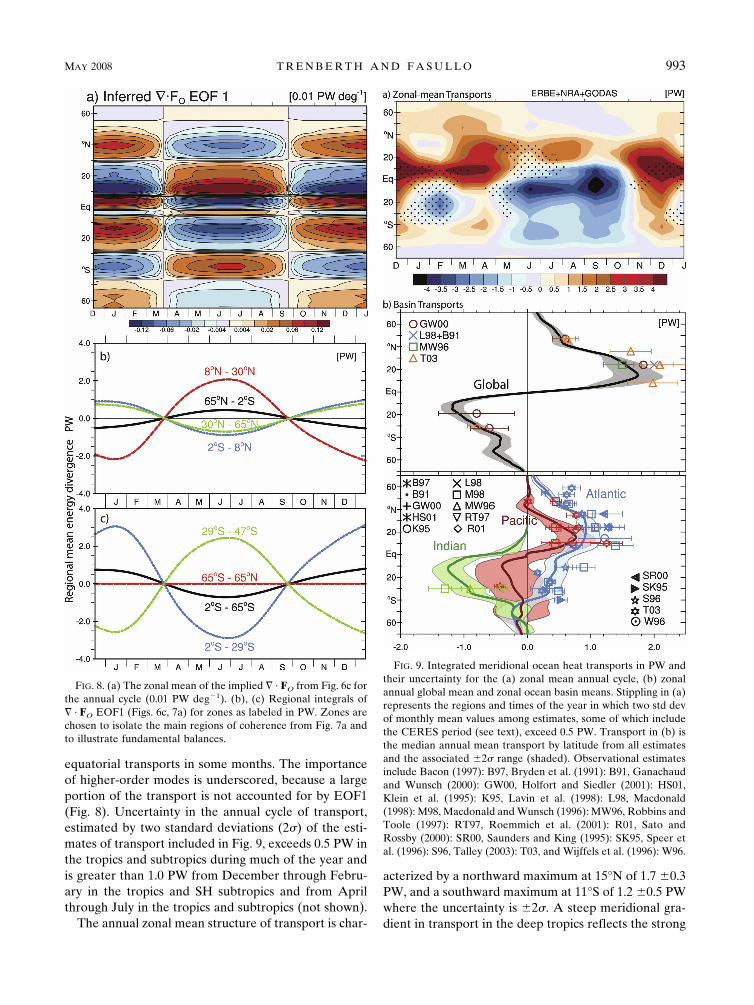
equatorial transports in some months. The importanceof higher-order modes is underscored, because a largeportion of the transport is not accounted for by EOF1(Fig. 8). Uncertainty in the annual cycle of transport,estimated by two standard deviations (2�) of the esti-mates of transport included in Fig. 9, exceeds 0.5 PW inthe tropics and subtropics during much of the year andis greater than 1.0 PW from December through Febru-ary in the tropics and SH subtropics and from Aprilthrough July in the tropics and subtropics (not shown).

The annual zonal mean structure of transport is char-

acterized by a northward maximum at 15°N of 1.7 0.3PW, and a southward maximum at 11°S of 1.2 0.5 PWwhere the uncertainty is 2�. A steep meridional gra-dient in transport in the deep tropics reflects the strong

FIG. 8. (a) The zonal mean of the implied � · FO from Fig. 6c forthe annual cycle (0.01 PW deg�1). (b), (c) Regional integrals of� · FO EOF1 (Figs. 6c, 7a) for zones as labeled in PW. Zones arechosen to isolate the main regions of coherence from Fig. 7a andto illustrate fundamental balances.

FIG. 9. Integrated meridional ocean heat transports in PW andtheir uncertainty for the (a) zonal mean annual cycle, (b) zonalannual global mean and zonal ocean basin means. Stippling in (a)represents the regions and times of the year in which two std devof monthly mean values among estimates, some of which includethe CERES period (see text), exceed 0.5 PW. Transport in (b) isthe median annual mean transport by latitude from all estimatesand the associated 2� range (shaded). Observational estimatesinclude Bacon (1997): B97, Bryden et al. (1991): B91, Ganachaudand Wunsch (2000): GW00, Holfort and Siedler (2001): HS01,Klein et al. (1995): K95, Lavin et al. (1998): L98, Macdonald(1998): M98, Macdonald and Wunsch (1996): MW96, Robbins andToole (1997): RT97, Roemmich et al. (2001): R01, Sato andRossby (2000): SR00, Saunders and King (1995): SK95, Speer etal. (1996): S96, Talley (2003): T03, and Wijffels et al. (1996): W96.


Fig 8 9 live 4/C

net energy flux into the ocean on the equator (Fig. 2).Despite the pronounced seasonal variability in cross-equatorial transports (Fig. 9a), the annual mean cross-equatorial transport is negligible (�0.1 PW), with anupper 2� bound of 0.6 PW.

The structure of global annual mean transports isgenerally supported by observed oceanographic sec-tions (Fig. 9), with close agreement at 47°N and 30°Sand agreement within the range of uncertainty at 24°N,8°N, and 20°S. At 36°N, the observed estimate of Talley(2003) exceeds the values derived here by about 0.6PW, which lies beyond the 20% (0.3 PW) error rangeprovided by Talley. Our NH northward transports aresystematically less than the ocean estimates between 0°and 40°N, and this bias occurs in the North Atlantic.

Mean transport in the Atlantic Ocean is northwardnorth of 40°S, while in the Indian Ocean, it is southwardat all latitudes. In the Pacific Ocean, transport is posi-tive in the NH and negative in the SH. As in Trenberthand Caron (2001), the magnitude of mean transports iscomparable among the basins, with a southward peakof 0.8 PW at 12°S in the Indian Ocean, a northwardpeak of 0.8 PW at 40°N in the Atlantic Ocean, andnorthward and southward peaks of 0.9 PW at 13°N and0.6 PW at 10°S, respectively, in the Pacific Ocean.

In the Atlantic, agreement with some direct oceanestimates is good, including those of Bacon (1997) at47°N, Speer et al. (1996) at 36°N, and Talley (2003) at8°N and 18°S. In other instances, disagreement betweenthe estimates is large, such as for Talley (2003) at 47°N,Macdonald (1998) at 8°N, and Speer et al. (1996) andMacdonald at 8°S, although in several of these casesthere are also disagreements among the direct oceanestimates that are outside the estimated error bars.Agreement with observed sections in the Pacific is goodfor Talley (2003) at 47°N and numerous estimates at30°N, and for both the Indian and Pacific basins at 30°S.At 10°N in the Pacific the two direct estimates of Mac-donald (1998) and Talley (2003) are at odds and ourvalue is in between. Uncertainty in transports, based onthe range of estimates derived herein, is largest in theIndian Ocean, where sampling of the upper ocean issparse (Locarnini et al. 2006), variability in FS is large,and the heat budget of the upper ocean is complex(Loschnigg and Webster 2000).

4. Discussion

While agreement between estimates of transport de-rived herein and those from ocean sections are reassur-ing, there is considerable uncertainty in both (e.g., Bry-den et al. 2005). Additionally, temporal sampling is anissue (Koltermann et al. 1999), as indicated, for in-

stance, by the variability of Florida Strait cable esti-mates of current transports (Baringer and Larsen 2001)and recent moored measurements at 26.5°N (Cunning-ham et al. 2007). Many direct ocean estimates are bi-ased toward spring and summertime. Similarly, in-stances in which disagreement between the estimatesare large does not preclude the validity of our analysis.Moreover, in some regions, such as in the tropical Pa-cific and northern Atlantic Oceans, the observationsthemselves are mutually inconsistent. In many in-stances where the observations are at odds, the trans-ports provided herein represent a reasonable compro-mise between the direct observed values. Hence, thecurrent analysis represents an important additional ba-sis for assessing ocean energy transports.

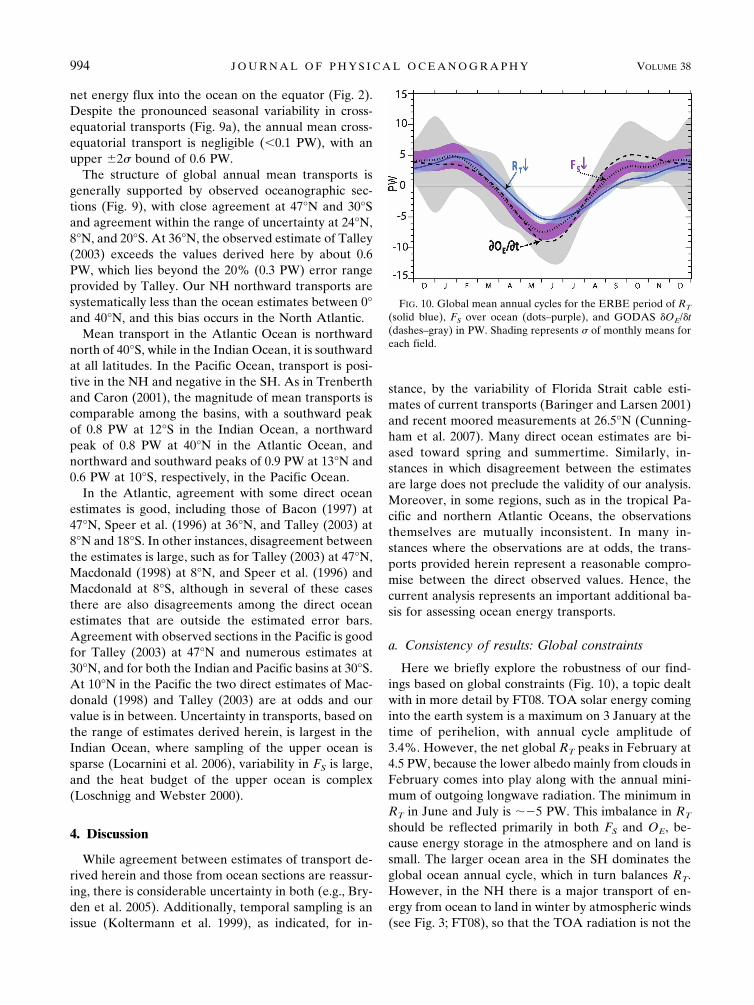
a. Consistency of results: Global constraints

Here we briefly explore the robustness of our find-ings based on global constraints (Fig. 10), a topic dealtwith in more detail by FT08. TOA solar energy cominginto the earth system is a maximum on 3 January at thetime of perihelion, with annual cycle amplitude of3.4%. However, the net global RT peaks in February at4.5 PW, because the lower albedo mainly from clouds inFebruary comes into play along with the annual mini-mum of outgoing longwave radiation. The minimum inRT in June and July is ��5 PW. This imbalance in RT

should be reflected primarily in both FS and OE, be-cause energy storage in the atmosphere and on land issmall. The larger ocean area in the SH dominates theglobal ocean annual cycle, which in turn balances RT.However, in the NH there is a major transport of en-ergy from ocean to land in winter by atmospheric winds(see Fig. 3; FT08), so that the TOA radiation is not the

FIG. 10. Global mean annual cycles for the ERBE period of RT

(solid blue), FS over ocean (dots–purple), and GODAS �OE/�t(dashes–gray) in PW. Shading represents � of monthly means foreach field.


Fig 10 live 4/C

only driver of FS over the oceans. Net evaporation overthe oceans and transport of latent energy to land areasresults in annual cycle variations in water (or snow andice) on land and sea level, as observed by altimetry(Minster et al. 1999), with amplitude equivalent to 9.5mm of sea level, peaking in September.

Globally, the difference between the TOA radiationand FS over ocean (Fig. 10) arises primarily from thesmall contributions from land storage tendency (FT08).Some energy storage also occurs in sea ice as an energydeficit in winter that is released in summer, althoughpresumably the energy tendency associated with sea icelargely cancels between the two hemispheres when in-tegrated globally. Hence, FS over ocean appears prin-cipally as a change in OE. The ocean temperaturedatasets imply a larger annual cycle of OE than FS es-timates do, and tendencies are outside the error bars insouthern winter (too low) and October–November (toohigh) (Fig. 10), and correspond to OE values that aretoo high in March–April and too low in August–Octo-ber. In FT08 and Fasullo and Trenberth (2008b) it isshown that the errors most likely arise from OE south of40°S, where WOA and JMA values are further astrayfrom GODAS, given in Fig. 10.

b. Ekman transports

The biggest differences between the results in Figs. 4and 6 and those of Antonov et al. (2004) are in thetropics, notably from �5° to 15°N, and especially in thePacific where there is strong evidence for the annualcycle being dominated by ocean dynamics. The zerowind stress curl line over the North Pacific migratesfrom 11°N in March to 20°N in September and inducesupper-layer thickness anomalies across the Pacific ba-sin, resulting in major seasonal changes in the NorthEquatorial Current (NEC) and where it bifurcatesalong the western boundary. The NEC is farthest northin October and farthest south in February (Qiu andLukas 1996). Furthermore, large seasonal changes inEkman transports lead to a substantial annual cycle innorthward energy transports throughout the tropics(Jayne and Marotzke 2001), and at 24°N (Zhang et al.2002) range from about zero in winter to maxima inJuly and November of 1 PW.

In the Atlantic, the NEC peaks in boreal summer andweakens during spring and fall (Arnault, 1987). Böningand Herrmann (1994) present results for a North At-lantic Ocean model simulation and the annual cycles ofsurface fluxes and OE show similar results to those pre-sented here. In the Atlantic at 8°N they also find a largeannual cycle in northward energy transports in whichthe strong NEC-induced changes in OE have little to dowith FS, but depend rather on changes in surface stress.

Kobayashi and Imasato (1998) determine that substan-tial annual cycles exist in meridional energy transportsin the Atlantic and Pacific, with the largest valuesaround 10°N. Seasonal variability in energy transport of100% is also suggested for the Indonesian Through-flow, and in the Indian Ocean the annual cycle justsouth of the equator is suggested to be �1.4 PW inDecember through February and �1.8 PW in Junethrough September (Loschnigg and Webster 2000). Theregional results are consistent with the inferred fieldspresented here.

For the total meridional transport at 24°N, Zhang etal. (2002) estimate that the annual cycle ranges from 1.1PW in February to 2.8 PW in August, with a mean of2.1 0.4 PW. The inference is that in both the Atlanticand Pacific transports enhance the annual cycle of OE

from what it would be based on FS alone by about 10%,as was shown for the Atlantic in a model by Böning andHerrmann (1994). While the transports at 24°N fromZhang et al. (2002) are consistent with the fields de-rived here, albeit somewhat stronger, generally the be-havior at 24°N is not representative of variability atother latitudes (Fig. 9), owing to the steep gradients intransport that exist in the subtropics seasonally andtheir complex relationship to cross-equatorial flow andmidlatitude variability, which is relatively weak. In-deed, in model simulations, Jayne and Marotzke (2001)demonstrate the dominant role of the annual cycle inEkman transports associated with broad overturningcirculations in the tropics and subtropics that contributeto strong energy transport and underlie the deducedchanges in OE. Based on the surface forcing they use,Ekman transports reverse sign sharply at about 25° lati-tude in each hemisphere through the course of the an-nual cycle. Hence, the dipole structures seen in Figs. 7and 8 near the tropics and midlatitudes in both hemi-spheres are qualitatively consistent with establishedchanges resulting from Ekman transports. Moreover,the suitability of assessing these transports near thenode of the overturning circulations, where the gradi-ent in transport is strong, is called into question.

c. Factors contributing to uncertainty

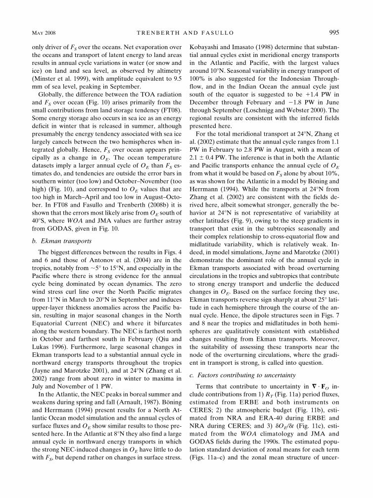
Terms that contribute to uncertainty in � · FO in-clude contributions from 1) RT (Fig. 11a) period fluxes,estimated from ERBE and both instruments onCERES; 2) the atmospheric budget (Fig. 11b), esti-mated from NRA and ERA-40 during ERBE andNRA during CERES; and 3) �OE/�t (Fig. 11c), esti-mated from the WOA climatology and JMA andGODAS fields during the 1990s. The estimated popu-lation standard deviation of zonal means for each term(Figs. 11a–c) and the zonal mean structure of uncer-


tainty in monthly means (Fig. 11d) are shown. The es-timates are independent (e.g., ERBE and CERESfluxes are not used in the compilation of the reanalysisor ocean datasets), and there is no expectation thatcancellation of uncertainty will occur when the fieldsare combined to infer � · FO. Because some of the dif-ferences between the fields in Fig. 11 represent realdifferences between the ERBE, CERES, and WOAtime periods, the estimates (Fig. 11) somewhat over-state the analysis uncertainty. At TOA, uncertainty as-sociated with RT is largest in the SH but it is still smallrelative to other terms (less than 0.01 PW deg�1). Un-certainty in � · FA, particularly in the tropics, is a sub-stantial contributor to the uncertainty in � · FO, withvalues exceeding 0.05 PW deg�1 from March throughNovember. Uncertainty associated with both the atmo-spheric budget and ocean tendencies is large in the sub-tropics, but near the node of EOF1 (Fig. 8) uncertaintyreturns to a relative minimum. In midlatitudes, largeuncertainty is associated primarily with disagreementsin estimates in the ocean tendencies; however, it de-creases toward the poles. In the extratropics, where themoisture-holding capacity of the atmosphere is greatlyreduced from that of the tropics, agreement between

ERA-40 and NRA estimates of � · FA is better anduncertainty is reduced. For the ocean, uncertainty as-sociated with �OE/�t is greatest in SH mid- to high lati-tudes and is likely to be associated with the lack ofobservations, and hence the reliance on infilling tech-niques used in constructing ocean analyses in these re-gions. Because the overall trend in ocean temperaturesis small across the 1990s, the annual zonal mean of�OE/�t is small compared to the other terms (Fasulloand Trenberth 2008b).

Together, the various contributions to uncertainty in� · FO represent a spatially complex pattern of diversecontributions with distinct underlying causes. Despiteuncertainty, the principle features of Fig. 7 are larger(order 0.2 PW deg�1) than the combined uncertainty ofterms in Fig. 11 (order 0.05 PW deg�1), and thus it islikely that its primary features are robust to data short-comings. A caveat to these conclusions would be ifthere is a substantial systematic error across all the es-timates for a particular field in Fig. 11. For instance,based on analysis of data from Argo floats, it has re-cently been suggested that WOA overstates the annualcycle in the North Atlantic Ocean (Ivchenko et al.2006) and perhaps globally (see also Willis et al. 2007).

FIG. 11. Uncertainty analysis of terms contributing to estimation of � · FO, including (a) RT, (b) � · FO � dAE/dt,(c) �OE/�t, and (d) the zonal means of the uncertainty in monthly means of each term (10�5 PW deg�1). Estimatesof uncertainty are based on the std dev among three estimates of each field, including (a) RT derived from periodsof ERBE and CERES (both instruments) fluxes, (b) estimates of � · FO and �AE/�t taken from NRA and ERA-40during ERBE, and NRA during CERES, and (c) estimates of �OE/�t from WOA fields, and from JMA andGODAS fields during the 1990s.


Fig 11 live 4/C

The potential presence of such biases is particularlylikely for ocean analyses, which share both similar ana-lytical bases and observational shortcomings. Revisionsof ocean datasets that have been suggested (Ivchenkoet al. 2006) would alter the values presented here.

5. Concluding remarks

A test of how well we understand the global energybudget of the earth system and the oceans is to examinethe annual cycle in detail and the degree to which clo-sure can be reached among a variety of independentdata. Significant advances in the observation and analy-sis of TOA, atmospheric, and ocean budgets have beenmade in recent decades such that the errors are nowrelatively modest and allow for an initial estimate ofocean energy divergence.

In midlatitudes, the seasonal ocean energy tendencyis dominated by surface fluxes, with divergence of en-ergy from ocean currents enhancing magnitudes by anorder of 50 W m�2. This finding is consistent withmodel results and is explained by Ekman transportsdriven by the annual cycle of surface winds. In contrast,in the tropics and subtropics, divergence is found toplay the dominant role in the upper-ocean energy bud-get with secondary but important contributions fromsurface fluxes.

The first mode of the annual cycle of divergence andthe dominant aspects of spatial coherence in this modeare identified and the total transports are calculated,globally and by basin. An additional important impli-cation is that the annual cycle of energy transports isprimarily a response to surface winds, rather than in-stabilities associated with temperature gradients, and itincreases seasonal energy extremes in the upper oceanand the amplitude of the annual cycle. This contrastswith the thermohaline circulation, which feeds on den-sity (and thus temperature) gradients.

Inferred annual mean ocean heat transports aresomewhat lower than direct ocean estimates in theNorth Atlantic, and thus the zonal average ocean. Al-though there are uncertainties in the atmospheric en-ergy transports, there is not much scope for the oceantransports to be increased because their sum is quitestrongly constrained. The fields used to infer ocean en-ergy divergence here are indirect and sensitive to theaccumulation of error through the depth of the atmo-sphere and oceans. While retrievals of radiative fluxesof TOA are among the most accurate fields to be ob-served globally, uncertainty in atmospheric divergenceand ocean energy tendency can be substantial, particu-larly on regional scales. With further refinements ofthese fields and more complete temporal sampling in

the ocean, a more accurate diagnosis of ocean energydivergence will be possible for comparison with model-assimilated fields from analysis of new ocean data. Withsufficient data and continued improvements, it will alsobe possible to extend these kinds of analyses to exam-ine interannual variability. This task has already beenrealized for the tropical Pacific to examine changes inenergy content with ENSO (Trenberth et al. 2002), al-though improvements in data quality continue to bedesirable. With new and improved TOA radiation datafrom the CERES and much better spatial and temporalresolution from global Argo float measurements, theprospects for doing this diagnosis routinely should be-come realistic. Accordingly, this approach has the po-tential to provide a more holistic view of the climatesystem, help validate ocean models, and better assessthe role of ocean energy uptake, release, and transportin climate variability.

Acknowledgments. This research is partially sponsoredby the NOAA CLIVAR and CCDD programs underGrants NA06OAR4310145 and NA07OAR4310051.We thank Bill Large, Frank Bryan, and Clara Deser forcomments, and Dave Stepaniak for help with compu-tations.

REFERENCES

Antonov, J. I., S. Levitus, and T. P. Boyer, 2004: Climatologicalannual cycle of ocean heat content. Geophys. Res. Lett., 31,L04304, doi:10.1029/2003GL018851.

Arnault, S., 1987: Tropical Atlantic geostrophic currents and shipdrifts. J. Geophys. Res., 92, 5076–5088.

Bacon, S., 1997: Circulation and fluxes in the North Atlantic be-tween Greenland and Ireland. J. Phys. Oceanogr., 27, 1420–1435.

Baringer, M. O., and J. C. Larsen, 2001: Sixteen years of FloridaCurrent transport at 27°N. Geophys. Res. Lett., 28, 3179–3182.

Barkstrom, B. R., and J. B. Hall, 1982: Earth Radiation BudgetExperiment (ERBE)—An overview. J. Energy, 6, 141–146.

Behringer, D. W., 2007: The Global Ocean Data Assimilation Sys-tem (GODAS) at NCEP. Proc. 11th Symp. on IntegratedObserving and Assimilation Systems for the Atmosphere,Oceans, and Land Surface (IOAS-AOLS), San Antonio, TX,Amer. Meteor. Soc., 3.3. [Available online at http://ams.confex.com/ams/pdfpapers/119541.pdf.]

——, and Y. Xue, 2004: Evaluation of the global ocean data as-similation system at NCEP: The Pacific Ocean. Proc. EighthSymp. on Integrated Observing and Assimilation Systems forAtmosphere, Oceans, and Land Surface, Seattle, WA, Amer.Meteor. Soc., 2.3. [Available online at http://ams.confex.com/ams/84Annual/techprogram/paper_70720.htm.]

Böning, C. W., and P. Herrmann, 1994: Annual cycle of polewardheat transport in the ocean: Results from high-resolutionmodeling of the North and equatorial Atlantic. J. Phys.Oceanogr., 24, 91–107.

Bryden, H. L., D. H. Roemmich, and J. A. Church, 1991: Ocean


heat-transport across 24°N in the Pacific. Deep-Sea Res., 38,297–324.

——, H. R. Longworth, and S. A. Cunningham, 2005: Slowing ofthe Atlantic meridional overturning at 25°N. Nature, 438,655–657.

Bunker, A. F., 1976: Computations of surface energy flux andannual air–sea interaction cycles of the North AtlanticOcean. Mon. Wea. Rev., 104, 1122–1140.

Cunningham, S. A., and Coauthors, 2007: Temporal variability ofthe Atlantic Meridional Overturning circulation at 26.5°N.Science, 317, 935–938.

Deser, C., M. A. Alexander, and M. S. Timlin, 1999: Evidence fora wind-driven intensification of the Kuroshio Current exten-sion from the 1970s to the 1980s. J. Climate, 12, 1697–1706.

Fasullo, J. T., and K. E. Trenberth, 2008a: The annual cycle of theenergy budget. Part I: Global mean and land–ocean ex-changes. J. Climate, 21, 2297–2313.

——, and ——, 2008b: The annual cycle of the energy budget. PartII: Meridional Structures and Poleward Transports. J. Cli-mate, 21, 2314–2326.

Ganachaud, A., and C. Wunsch, 2000: Improved estimates ofglobal ocean circulation, heat transport and mixing from hy-drographic data. Nature, 408, 453–457.

Grist, J. P., and S. A. Josey, 2003: Inverse analysis adjustment ofthe SOC air–sea flux climatology using ocean heat transportconstraints. J. Climate, 16, 3274–3295.

Hansen, J., and Coauthors, 2005: Earth’s energy imbalance: Con-firmation and implications. Science, 308, 1431–1435.

Holfort, J., and G. Siedler, 2001: The meridional oceanic trans-ports of heat and nutrients in the South Atlantic. J. Phys.Oceanogr., 31, 5–29.

Huang, S., 2006: Land warming as part of global warming. Eos,Trans. Amer. Geophys. Union, 87, 477.

Ishii, M., M. Kimoto, K. Sakamoto, and S. I. Iwasaki, 2006: Stericsea level changes estimated from historical ocean subsurfacetemperature and salinity analyses. J. Oceanogr., 62, 155–170.

Ivchenko, V. O., N. C. Wells, and D. L. Aleynik, 2006: Anomalyof heat content in the northern Atlantic in the last 7 years: Isthe ocean warming or cooling? Geophys. Res. Lett., 33,L22606, doi:10.1029/2006GL027691.

Jayne, S. R., and J. Marotzke, 2001: The dynamics of ocean heattransport variability. Rev. Geophys., 39, 385–411.

Kistler, R., and Coauthors, 2001: The NCEP–NCAR 50-Year Re-analysis: Monthly means CD-ROM and documentation. Bull.Amer. Meteor. Soc., 82, 247–267.

Klein, B., R. L. Molinari, T. J. Muller, and G. Siedler, 1995: Atransatlantic section at 14.5n—Meridional volume and heatfluxes. J. Mar. Res., 53, 929–957.

Kobayashi, T., and N. Imasato, 1998: Seasonal variability of heattransport derived from hydrographic and wind stress data. J.Geophys. Res., 103, 24 663–24 674.

Köberle, C., and R. Gerdes, 2003: Mechanisms determining thevariability of Arctic sea ice conditions and export. J. Climate,16, 2843–2858.

Koltermann, K. P., A. V. Sokov, V. P. Tereschenkov, S. A. Do-broliubov, K. Lorbacher, and A. Sy, 1999: Decadal changes inthe thermohaline circulation of the North Atlantic. Deep-SeaRes. II, 46, 109–138.

Lavin, A., H. L. Bryden, and G. Parrilla, 1998: Meridional trans-port and heat flux variations in the subtropical North Atlan-tic. Global Atmos. Ocean. Syst., 6, 269–293.

Levitus, S., 1984: Annual cycle of temperature and heat storage inthe World Ocean. J. Phys. Oceanogr., 14, 727–746.

——, 1987: Rate of change of heat storage in the World Ocean. J.Phys. Oceanogr., 17, 518–528.

——, and J. Antonov, 1997: Climatological and Interannual Vari-ability of Temperature, Heat Storage, and Rate of Heat Stor-age in the World Ocean. NOAA Atlas NESDIS 16, 6 pp.�186figs.

——, ——, and ——, 2005: Warming of the world ocean, 1955–2003. Geophys. Res. Lett., 32, L02604, doi:10.1029/2004GL021592.

Locarnini, R. A., A. V. Mishonov, J. I. Antonov, T. P. Boyer, andH. E. Garcia, 2006: Temperature. Vol. 1, World Ocean Atlas2005, NOAA Atlas NESDIS 61, 182 pp.

Loeb, N. G., and Coauthors, 2007: Multi-instrument comparisonof top-of-atmosphere reflected solar radiation. J. Climate, 20,575–591.

Loschnigg, J., and P. J. Webster, 2000: A coupled ocean–atmo-sphere system of SST modulation for the Indian Ocean. J.Climate, 13, 3342–3360.

Macdonald, A. M., 1998: The global ocean circulation: A hydro-graphic estimate and regional analysis. Prog. Oceanogr., 41,281–382.

——, and C. Wunsch, 1996: An estimate of global ocean circula-tion and heat fluxes. Nature, 382, 436–439.

Minster, J. F., A. Cazenave, Y. V. Serafini, F. Mercier, M. C. Gen-nero, and P. Rogel, 1999: Annual cycle in mean sea level fromTopex-Poseidon and ERS-1: Inference on the global hydro-logical cycle. Global Planet. Change, 20, 57–66.

Moisan, J. R., and P. P. Niiler, 1998: The seasonal heat budget ofthe North Pacific: Net heat flux and heat storage rates (1950–1990). J. Phys. Oceanogr., 28, 401–421.

Qiu, B., and R. Lukas, 1996: Seasonal and interannual variabilityof the North Equatorial Current, the Mindanao Current, andthe Kuroshio along the Pacific western boundary. J. Geophys.Res., 101, 12 315–12 330.

Robbins, P. E., and J. M. Toole, 1997: The dissolved silica budgetas a constraint on the meridional overturning circulation ofthe Indian Ocean. Deep-Sea Res., 44, 879–906.

Roemmich, D., J. Gilson, B. Cornuelle, and R. Weller, 2001:Mean and time-varying meridional transport of heat at thetropical subtropical boundary of the North Pacific Ocean. J.Geophys. Res., 106, 8957–8970.

Sato, O. T., and T. Rossby, 2000: Seasonal and low-frequencyvariability of the meridional heat flux at 36° N in the NorthAtlantic. J. Phys. Oceanogr., 30, 606–621.

Saunders, P. M., and B. A. King, 1995: Oceanic fluxes on theWOCE A11 section. J. Phys. Oceanogr., 25, 1942–1958.

Serreze, M. C., and Coauthors, 2006: The large-scale freshwatercycle of the Arctic. J. Geophys. Res., 111, C11010,doi:10.1029/2005JC003424.

——, A. P. Barrett, A. G. Slater, M. Steele, J. Zhang, and K. E.Trenberth, 2007: The large-scale energy budget of the Arctic.J. Geophys. Res., 112, D11122, doi:10.1029/2006JD008230.

Speer, K. G., J. Holfort, T. Reynard, and G. Siedler, 1996: SouthAtlantic heat transport at 11°S. The South Atlantic: Presentand Past Circulation, G. Wefer, G. Siedler, and D. J. Webb,Eds., Springer, 105–120.

Talley, L. D., 2003: Shallow, intermediate, and deep overturningcomponents of the global heat budget. J. Phys. Oceanogr., 33,530–560.

Trenberth, K. E., 1997: Using atmospheric budgets as a constrainton surface fluxes. J. Climate, 10, 2796–2809.

——, and J. M. Caron, 2001: Estimates of meridional atmosphereand ocean heat transports. J. Climate, 14, 3433–3443.


——, and D. P. Stepaniak, 2003a: Covariability of components ofpoleward atmospheric energy transports on seasonal and in-terannual timescales. J. Climate, 16, 3690–3704.

——, and ——, 2003b: Seamless poleward atmospheric energytransports and implications for the Hadley circulation. J. Cli-mate, 16, 3705–3721.

——, and ——, 2004: The flow of energy through the Earth’sclimate system. Quart. J. Roy. Meteor. Soc., 130, 2677–2701.

——, J. M. Caron, and D. P. Stepaniak, 2001: The atmosphericenergy budget and implications for surface fluxes and oceanheat transports. Climate Dyn., 17, 259–276.

——, D. P. Stepaniak, and J. M. Caron, 2002: Interannual varia-tions in the atmospheric heat budget. J. Geophys. Res., 107,4066, doi:10.1029/2000JD000297.

Uppala, S. M., and Coauthors, 2005: The ERA-40 reanalysis.Quart. J. Roy. Meteor. Soc., 131, 2961–3012.

Wielicki, B. A., B. R. Barkstrom, E. F. Harrison, R. B. Lee, G. L.Smith, and J. E. Cooper, 1996: Clouds and the Earth’s Radi-ant Energy System (CERES): An earth observing systemexperiment. Bull. Amer. Meteor. Soc., 77, 853–868.

——, K. Priestley, P. Minnis, N. Loeb, D. Kratz, T. Charlock, D.Doelling, and D. Young, 2006: CERES radiation budget ac-

curacy overview. Preprints, 12th Conf. on Atmospheric Ra-diation, Madison, WI, Amer. Meteor. Soc., 9.1. [Availableonline at http://ams.confex.com/ams/Madison2006/techprogram/paper_112371.htm.]

Wijffels, S. E., J. M. Toole, H. L. Bryden, R. A. Fine, W. J. Jen-kins, and J. L. Bullister, 1996: The water masses and circula-tion at 10°N in the Pacific. Deep-Sea Res. I, 43, 501–544.

Willis, J. K., D. Roemmich, and B. Cornuelle, 2004: Interannualvariability in upper ocean heat content, temperature, andthermosteric expansion on global scales. J. Geophys. Res.,109, C12036, doi:10.1029/2003JC002260.

——, J. M. Lyman, G. C. Johnson, and J. Gilson, 2007: Correctionto “Recent cooling of the upper ocean.” Geophys. Res. Lett.,34, L16601, doi:10.1029/2007GL030323.

Yan, X.-H., P. P. Niiler, S. K. Nadiga, R. Stewart, and D. Cayan,1995: The seasonal heat storage in the North Pacific. J. Geo-phys. Res., 100, 6899–6926.

Zhang, D., W. E. Johns, and T. N. Lee, 2002: The seasonal cycle ofmeridional heat transport at 24°N in the North Pacific and inthe global ocean. J. Geophys. Res., 107, 3083, doi:10.1029/2001JC001011.


Documents

An Observational Estimate of Inferred Ocean Energy Divergence