A

pstaofssp©

K

1

ff

F

0

Available online at www.sciencedirect.com

Mathematics and Computers in Simulation 82 (2012) 909–923

Original article

An optimal control methodology for plant growth—Case study of awater supply problem of sunflower

Lin Wu a,b,∗, Francois-Xavier Le Dimet c,d, Philippe de Reffye e,f, Bao-Gang Hu g,Paul-Henry Cournède e,h, Meng-Zhen Kang g

a Université Paris-Est, CEREA, joint laboratory Ecole des Ponts ParisTech – EDF R&D, Marne la Vallée F-77455, Franceb INRIA, Clime, Rocquencourt F-78153, France

c Université Joseph Fourier, Lab. Jean Kuntzmann (LJK), Grenoble F-38041, Franced INRIA, MOISE, Grenoble F-38041, Francee INRIA, DigiPlante, Orsay F-91893, France

f CIRAD, UMR AMAP, Montpellier F-34000, Franceg Chinese Academy of Sciences, Institute of Automation, LIAMA, Beijing 100080, China

h Ecole Centrale Paris, Laboratory of Applied Mathematics, Châtenay-Malabry F-92295, France

Received 17 December 2010; received in revised form 13 November 2011; accepted 22 December 2011Available online 18 January 2012

bstract

An optimal control methodology is proposed for plant growth. This methodology is demonstrated by solving a water supplyroblem for optimal sunflower fruit filling. The functional–structural sunflower growth is described by a dynamical system givenoil water conditions. Numerical solutions are obtained through an iterative optimization procedure, in which the gradients ofhe objective function, i.e. the sunflower fruit weight, are calculated efficiently either with adjoint modeling or by differentiationlgorithms. Further improvements in sunflower yield have been found compared to those obtained using genetic algorithms inur previous studies. The optimal water supplies adapt to the fruit filling. For instance, during the mid-season growth, the supplyrequency condenses and the supply amplitude peaks. By contrast, much less supplies are needed during the early and ending growthtages. The supply frequency is a determining factor, whereas the sunflower growth is less sensitive to the time and amount of onepecific irrigation. These optimization results agree with common qualitative agronomic practices. Moreover they provide morerecise quantitative control for sunflower growth.

2012 IMACS. Published by Elsevier B.V. All rights reserved.

eywords: Functional–structural plant model; Dynamical system; Optimal control; Adjoint model

. Introduction

Functional–structural plant models (FSPMs [33,34,28]) combine process-based models and architectural modelsor better description of plant growth. The process-based models characterize plant mechanisms like photosynthesisor agronomic applications [24,8]. By contrast, the architectural models were originally developed to analyze botanic

∗ Corresponding author at: Université Paris-Est, CEREA, joint laboratory Ecole des Ponts ParisTech – EDF R&D, Marne la Vallée F-77455,rance.

E-mail address: Lin.Wu@cerea.enpc.fr (L. Wu).

378-4754/$36.00 © 2012 IMACS. Published by Elsevier B.V. All rights reserved.doi:10.1016/j.matcom.2011.12.007

910 L. Wu et al. / Mathematics and Computers in Simulation 82 (2012) 909–923

patterns [14] or topological structures [32]. A typical FSPM can thus simulate not only plant organogenesis, but alsobiomass production and partition at organ level (leaf, internode, fruit, etc.). This leads to many FSPM applications,such as breeding and yield optimization [20,29].

Several FSPMs have been proposed, e.g. GROGRA [17], LIGNUM [27], L-systems variants [26], and GreenLab[39,7]. An interesting GreenLab characteristic is that it simulates the plant functional–structural growth by a mathe-matical recursive algorithm formulated as dynamical equations. This growth algorithm is based on a minimal set ofphysiological knowledge, such as the empirical rules of plant–environment interactions for biomass acquisition and thesource–sink relations among organs that compete for assimilates. Consequently, the plant morphological plasticity canbe described with a small set of endogenous parameters. The complexity of parameter calibrations is thus reduced [12].The usability of GreenLab for practical applications has been justified by the resulting stable calibrated parameterscross phenotypic plasticity [22]. The main challenging issue of FSPMs is the balance between mathematical clarityand physiological complexity.

The mathematical transparency of GreenLab makes it natural to be formulated as a discrete dynamicalsystem:

{x(n) = F (x(n − 1), �, u(n − 1)),

x(0) = ϒ,(1)

where n is the time index, F is a nonlinear operator, x is the state vector, ϒ is the initial state at time step n = 0, u isthe input data or control vector, and � is the set of model endogenous parameters. The solution of Eq. (1) gives thetrajectory of system state, with which different types of problems can be defined [38]. For example, the calibrationproblem is to find optimal � to minimize the discrepancy between model simulations and experimental observations.The state estimation problem is to retrieve the state status by optimizing the phenotype-specific parameters such as theexogenous input data U and the initial state ϒ. Whereas the control problem is to find U, sometimes also � and ϒ,to optimize a given objective or criterion, e.g. the yield. These formulations are still not well recognized in the FSPMcommunity.

The FSPM control problem is a difficult issue because of the nonlinearity of the plant system. In many caseseven discontinuity is involved. This nonlinearity is due to the biological thresholding or saturation effects. It pro-hibits exact analytical solutions of the control problem. Heuristic searching methods based on GreenLab have beenproposed for numerical solutions [38,29]. These methods are simulation-based; the plant system is treated as ablack-box model. As a result, the advantage of the mathematical transparency of GreenLab unfortunately fadesout. Furthermore, they scale badly with the dimension of the control parameter space and suffer from the curse ofdimensionality.

In this paper, we propose an optimal control methodology for plant functional–structural growth, in which thegradient of the objective function can be efficiently computed by adjoint modeling [21,19]. This makes it feasible tosolve the plant control problem using classic descent algorithms. Contrary to the heuristic methods, this methodologyscales well with the large-scale systems, e.g. those in atmospheric science of which the dimension of state vectorusually goes beyond a million [30,37].

This optimal control methodology is demonstrated by solving a sunflower water supply problem. This irrigationproblem has been investigated in our previous study using a genetic algorithm in which only four parameters arecontrolled [38]. In this study, much more exogenous control parameters will be optimized. Note that we are not aimingat an operational solution of a practical irrigation problem, but rather an evaluation of the performance of this optimalcontrol methodology. Yet hopefully some physiological insights could be inferred by examining the resulting optimalwater supplies.

The paper is organized as follows. In Section 2, each component in Eq. (1) is explicitly specified for ourplant–soil dynamical system. The optimal control methodology for the sunflower water supply problem is pre-

sented in Section 3, in which is derived the adjoint model of the control system, as well as the practicalcalculation of gradients using differential algorithms. The solution of the optimal watering problem is givenwith physiological interpretation in Section 4. A general discussion as well as perspectives are given in the lastsection.

L. Wu et al. / Mathematics and Computers in Simulation 82 (2012) 909–923 911

2

ca

2

uat

ect

wae

jc

wsh

w[

Fig. 1. Schematic of plant functional–structural growth [43] under soil water conditions.

. Dynamics formulation

In this section, we present how plant growth can be described by discrete dynamical equations. Detailed botaniconcepts and physiological knowledge can be found in [32,39]. The soil moisture model and its interaction with plantre treated in the same way as in [38].

.1. Functional–structural plant growth in interaction with soil water conditions

We formulate plant growth at organ level. The functional–structural growth is sketched in Fig. 1. Plant is assumed tondergo Growth Cycles (GCs) of a biological clock. During each GC the plant metabolism results in the emergence of

cohort of new organs. The GC can vary from several days (cottons) to one year (trees of temperate regions). However,he sum of the daily temperatures during the GC is assumed to be quite constant [31].

At every GC, the plant produces biomass by leaf photosynthesis. If the microclimatic environment conditions aroundach leaf are identical, then Q(n), the biomass produced by the photosynthesis of all the leaves during GC n, can bealculated by an empirical nonlinear function Ψ with respect to the environmental conditions, the number of leaves,he leaf surface areas, and some hidden parameters. In [39], the nonlinear function is chosen as

Q(n) = Ψ (S, E, r1, r2) =n∑

a=1

(Nl(a, n) · E(n)

(r1/S(a, n)) + r2

), (2)

here Nl(a, n) is the number of leaves of Chronological Age a (CA, counted by GCs) at GC n, S(a, n) is their surfacerea, r1, r2 are hidden parameters to be assessed, E(n) is the average biomass production potential depending onnvironmental conditions, such as light, temperature and soil water content.

For each organ, we define its demand as its ability to attract biomass. The organ demand do depends on organ CA and organ type o (o = l, e, c, f, m refers respectively to leaf, internode, layer, female flower and male flower), and isalculated as

do(j) = Poφo(j), (3)

here Po are the organ sink strengths, φo are normalized distribution functions characterizing the evolution of the sinktrengths from CA 1 to CA to with to being the organ lifespan. In this study, φos are chosen to be beta functions withidden function parameters. The total biomass demand of all plant organs at GC n is as

D(n) =∑ to∑

No(a, n) · do(a), (4)

o a=1

here No(a, n) is the number of o-type organs of CA a at GC n. The organ numbers can be calculated by automaton39] or botanic growth grammar [36, Ch. 2].

912 L. Wu et al. / Mathematics and Computers in Simulation 82 (2012) 909–923

The biomass produced by photosynthesis is redistributed among all organs according to the ratio between theirdemands do with respect to total plant demand D(n). This instantaneously leads to the calculation of the biomassincrement �qo(a, n) and total cumulated biomass qo(a, n) for any o-type organ of CA a at the current GC n:

�qo(a, n) = do(a)

D(n)· Q(n − 1),

qo(a, n) =a∑

j=1

�qo(j, n − (a − j)) = Po

a∑j=1

φo(j) · Q(n − (a − j) − 1)

D(n − (a − j)).

(5)

Given plant geometry configurations (organ shape and size, phyllotaxy), we can thus construct 3D plants through Eq.(5).

The biomass production potential E during GC n is supposed to be linearly proportional to the current soil watercontent. The light, temperature, and mineral conditions are assumed to be optimal and the plant suffers from no stress(for a complete formula, see [36]):

E(n) =

⎧⎪⎪⎨⎪⎪⎩0 Qw(n) ≤ Qwmn,

κ · Qw(n) − Qwmn

β(Qwmx − Qwmn)Qwmn < Qw(n) ≤ (1 − β)Qwmn + βQwmx,

κ Qw(n) > (1 − β)Qwmn + βQwmx,

(6)

where Qw(n) is the soil water content at GC n, Qwmn corresponds to the wilt point of soil water content beneathwhich the plant cannot extract water from soil, Qwmx is the water field capacity above which the water flows away,and κ is an empirical parameter. Plant suffers from water stress when (Qw(n) − Qwmn)/(Qwmx − Qwmn) < β withβ = 0.4. The thresholds here make the system strongly nonconvex. The biomass production potential formula Eq.(6) is a simplified account of the plant–soil system for the test of our optimal control methodology. More complexdescriptions are possible. For instance, precise extinction law could be employed based on adjusted leaf area index(LAI) to account for plant populational products [12], and realistic water stress model could also be introduced [23].However, mathematically it does not change much the underlying optimal control problem.

Plants participate in soil water circulation by transpiration. Water is taken from soil by roots and flows through theplant hydraulic network up to the leaves, where water is transpired to provide necessary energy fluxes for photosynthesis.The water content in the superior soil layers, named soil moisture, is important for the study of bio-geophysical processesin agricultural or forestry ecosystems. Soil water balance is achieved when we simplify this complex soil–plant systemby concentrating on plant transpiration, soil evapotranspiration, and water supply from both irrigation and precipitations.The soil water content in soil per surface unit (Qw) is calculated by the difference equation [38]:

Qw(n) − Qw(n − 1) = −c1(Qw(n − 1) − Qwmn)︸ ︷︷ ︸soil evapotranspiration

+ c2(Qwmx − Qw(n − 1))U(n − 1)︸ ︷︷ ︸water absorption

− ρ · Q(n − 1)︸ ︷︷ ︸plant transpiration

, (7)

where U(n − 1) (a scalar) is the water supply during GC n − 1, c1 is an evapotranspiration coefficient, and c2 is anabsorption coefficient. The plant transpiration is assumed to be linearly proportional to biomass production [15], andρ is the ratio between plant transpiration and plant biomass production during GC n − 1.

2.2. Dynamical system

Supposing constant mass per unit area ε, the leaf surface area S(a, n) can be calculated by dividing leaf mass ql(a,n) by ε. Substituting S(a, n) into Eq. (2), we have a recursive equation for the total biomass produced at GC n withoutexplicitly calculating the geometrical sizes of the leaves [39]:

Q(n) = E(n) ·tw∑

a=1

Nl(a, n) ·∑aj=1

φl(j) · Q(n−(a−j)−1)D(n−(a−j))

A + B ·∑aj=1

φl(j) · Q(n−(a−j)−1)D(n−(a−j))

. (8)

Ha

w

wnco

ws

3

3

lt

a

wa

L. Wu et al. / Mathematics and Computers in Simulation 82 (2012) 909–923 913

ere A = r1ε/Pl, B = r2, and tw is the leaf functioning period for photosynthesis. Let x(n − 1), x(n) be the state vectort GC n − 1 and n respectively:

x(n − 1) =

⎡⎢⎢⎢⎢⎢⎢⎢⎣

Q(n − tw)...

Q(n − 2)

Q(n − 1)

Qw(n − 1)

⎤⎥⎥⎥⎥⎥⎥⎥⎦, x(n) =

⎡⎢⎢⎢⎢⎢⎢⎢⎣

Q(n − tw + 1)...

Q(n − 1)

Q(n)

Qw(n)

⎤⎥⎥⎥⎥⎥⎥⎥⎦.

e can then rewrite the soil–plant system (6)–(8) in one difference equation:⎧⎪⎪⎪⎪⎪⎪⎪⎪⎨⎪⎪⎪⎪⎪⎪⎪⎪⎩

xj(n) = xj+1(n − 1), j = 1, . . . , tw − 1,

xtw (n) = κ · xtw+1(n) − Qwmn

β(Qwmx − Qwmn)

tw∑a=1

Nl(a, n) ·∑aj=1

φl(j) · xtw−a+j(n − 1)

D(n − (a − j))

A + B ·∑aj=1

φl(j) · xtw−a+j(n − 1)

D(n − (a − j))

,

xtw+1(n) = (1 − c1 − c2 · U(n − 1))xtw+1(n − 1) + Qwmnc1 + Qwmxc2 · U(n − 1) − ρ · xtw (n − 1),

(9)

here the superscripts of x denote the index of its components, the control vector U(n − 1) is the water supply at GC − 1. The endogenous parameter set � is composed of hidden parameters r1, r2, Po, φo and soil moisture parameters1, c2. Note that in system (9), only Pl and φl are used. However, Po and φo are also needed to compute the biomassf o-type organ. The initial condition is

x(0) = ϒ =

⎡⎢⎢⎢⎢⎢⎢⎢⎣

0...

0

Q0

Qw0

⎤⎥⎥⎥⎥⎥⎥⎥⎦, (10)

here Q0 is seed biomass, and Qw0 is the initial soil water content. This completes the detailed formulation of dynamicalystem Eq. (1) for our water supply problem.

. Optimal control methodology

.1. An optimal control problem for sunflower water supply

The sunflower water supply problem is to find optimal irrigation strategies for maximal fruit production underimited water resource conditions. We chose a 63 GC sunflower growth. The hidden parameters in � are set accordingo calibration results [40,13]. The soil moisture parameters c1, c2 are set to empirical values from previous studies.

Substituting the biomass production Q by the corresponding component of state vector x, we rewrite the fruitccumulated biomass Eq. (5) as follows:

qf (tf , N) =tf∑

�qf (j, N) = Pf

tf∑φf (j) · xtw (N − (tf − j) − 1), (11)

j=1 j=1D(N − (tf − j))

here N is the number of total sunflower growth GCs, and tf is the fruit CA. In the sunflower simulation, N = 63 GC,nd fruit appears at 38 GC thus tf = 63 − 38 = 25 GC.

914 L. Wu et al. / Mathematics and Computers in Simulation 82 (2012) 909–923

For convenience, hereafter the GC numbers are moved to subscript of the vectors, e.g. xn for x(n). If we define afunction l as{

l(xn, Un) = �qf (N − n, N), n ≥ N − tf ,

l(xn, Un) = 0, n < N − tf ,(12)

then the final fruit biomass production can be formulated as a function:

J(U) = qf (tf , N) =N−1∑n=0

l(xn, Un), (13)

where U = [U0, . . . , UN−1]T ∈ RN is the water supply vector of 63 dimension for all GCs. Here T denotes the transpose

of a vector or a matrix. The maximal fruit biomass production with respect to water supply U is the solution of thefollowing optimal control system:{

xn = F (xn−1, �, Un−1),

x0 = ϒ,

argmaxU∈RN

J(U),(14)

where F is a vector function of (tw + 1) dimension. In numerous cases, water resources are limited due to drought oreconomic reasons. We thus suppose the water supplies are under the following constraints,⎧⎪⎪⎨⎪⎪⎩

N−1∑i=0

Ui ≤ Π,

Ui ≥ 0,

i = 0, . . . , N − 1, (15)

where Π is a given total quantity of water supply during the sunflower growth.

3.2. Descent algorithms

The numerical solution of the optimal control problem Eq. (14) can be obtained by descent algorithms, in which aseries of points {Uk, k = 0, 1, 2, . . .} can be constructed by

Uk+1 = Uk + αkdk, (16)

where dk is the direction along which Uk+1 a better objective function value than Uk can be found. The iteration stepαk can be determined by the following unidimensional optimization problem,

αk = argmaxα

J(Uk + αdk) (17)

The maximization problem can be converted into a minimization problem by simply inverting the sign of J. Inthis case dk is a descent direction. A popular choice of dk is the steepest descent direction which is the negativegradient of the objective function. More complicated choices are possible, e.g. the quasi-Newton methods [3]. Mostefficient optimization methods are based on gradients [10]. In this study, a descent algorithm, the sequential quadraticprogramming (SQP) [2], in which quadratic subproblems are constructed, is used to solve our constrained optimizationproblem. The iterations stop when directional derivatives along searching direction dk tend to zero. It is importantto note that, because of the high nonconvexity of the plant model, the convergence of the descent methods is notguaranteed, and the solutions can be local optima.

3.3. Adjoint model for gradient calculations

The optimal control methodology provides efficient techniques to compute the gradients of the objective functionby introducing the adjoint model of the original dynamical model [21,19].

pp

E

Hc

t

TcdC

m

3

id

L. Wu et al. / Mathematics and Computers in Simulation 82 (2012) 909–923 915

Suppose that Un, xn are p-dimensional and m-dimensional vectors respectively. For our water supply problem, = 1 and m = tw + 1. The first-order variations in the state vector x and the objective function J resulting from aerturbation U on the control vector U, denoted as x and J, can be derived as follows⎧⎨⎩ xn+1 = ∂F

∂x(xn, Un)xn + ∂F

∂U(xn, Un)Un,

x0 = 0,(18)

J =N−1∑n=0

(∂l

∂x(xn, Un)xn + ∂l

∂U(xn, Un)Un

)=

N−1∑n=0

(∂l

∂x(xn, Un)xn

)+

N−1∑n=0

(∂l

∂U(xn, Un)Un

). (19)

q. (18) is the so-called tangent linear model. Let Mi×j denote the set of matrices with i rows and j columns, we have

∂F

∂x= [aij]m×m ∈ M

m×m, xn ∈ Mm×1;

∂F

∂U∈ M

m×p, Un ∈ Mp×1;∂l

∂x∈ M

1×m,∂l

∂U∈ M

1×p.

ere each component aij of the Jacobian matrix ∂F/∂x is a partial derivative of ith function of F with respect to jthomponent of state vector x.

If we define a vector of adjoint variables xn that are governed by the following adjoint model⎧⎪⎨⎪⎩xn =[∂F

∂x(xn, Un)

]T

xn+1 +[

∂l

∂x(xn, Un)

]T

,

xN = 0,

n = N − 1, . . . , 0, (20)

hen the gradient ∇J with respect to U can be calculated as

∇J =

⎡⎢⎢⎢⎢⎢⎢⎢⎣

[∂F

∂U(x0, U0)

]T

x1 +[

∂l

∂U(x0, U0)

]T

...[∂F

∂U(xN−1, UN−1)

]T

xN +[

∂l

∂U(xN−1, UN−1)

]T

⎤⎥⎥⎥⎥⎥⎥⎥⎦. (21)

he detailed derivation of the gradient formula (21) is presented in Appendix A. This gradient formula is for the generalase, in which the function l in system (14) depends on both xn and Un. For our specific case, the function l in Eq. (12)oes not depend on U explicitly, therefore ∂l/∂U equals zero. Note that the adjoint variable x is zero at n = N: xN = 0.onsequently the gradient formula becomes:

∇J =

⎡⎢⎢⎢⎢⎢⎢⎢⎢⎢⎣

[∂F

∂U(x0, U0)

]T

x1

...[∂F

∂U(xN−2, UN−2)

]T

xN−1

0

⎤⎥⎥⎥⎥⎥⎥⎥⎥⎥⎦. (22)

The optimality system is defined as the aggregation of the dynamical model and objective function (14), the adjointodel (20), and the gradient formula (21) (see [18] for more discussions on the optimality system).

.4. Differentiation algorithm to generate the adjoint code for gradient calculations

The main difficulty is to implement the adjoint model. In most cases, the derivation of the adjoint model and itsmplementation, as presented in the previous section, are time-consuming and error-prone especially for complexynamical models. Nowadays, almost all the complex models are implemented as computer programs. An alternative

916 L. Wu et al. / Mathematics and Computers in Simulation 82 (2012) 909–923

approach is to obtain directly the code of adjoint models based on the code of original dynamical models. This can becarried out either following some coding conventions [35] or using an automatic differentiation software [11].

Now we show how a systematic approach can be conducted to obtain the adjoint code for our water supply problem.Let

Jn =n−1∑i=0

l(xi, Ui), (23)

and let Xn = [U, xn, Jn]T be the augmented state vector of N + m + 1 dimension, we have the following dynamicalsystem:

Xn = Mn(Xn−1), n = 1, . . . , N, (24)

where Mn is the function that maps Xn−1 to Xn according to the plant dynamics Eq. (14) and the fruit accumulationEq. (23). The initial condition of this system is: X0 = [U, x0, J0]T.

Applying (24) from GC 1 to N successively, we get

XN = MN (MN−1(· · ·M1(X0)· · ·)). (25)

Perturbing U by U, the tangent linear model of direct model (24) can be obtained:

Xn = AnXn−1, n = 1, . . . , N, (26)

where An is the linearized form of Mn. Denoting P = [IN 0]T ∈ M(N+m+1)×N , where 0 is zero matrix, and IN stands

for N-by-N identity matrix, we have X0 = PU. Repeatedly applying tangent linear model (26) from GC 1 to N leadsto:

XN = ANAN−1· · ·A1PU. (27)

Denote Q = [0 1] ∈ M1×(N+m+1), and note that J = JN , we have:

J = QXN = 〈QT, XN〉RN+m+1 , (28)

where 〈〉RN+m+1 is the inner product in Euclidean space RN+m+1.

Let us define the adjoint operator A* of a linear operator A by

〈x, Ay〉E = 〈A∗x, y〉F, (29)

where x ∈ E, y ∈ F. Here E, F are Euclidean spaces equipped with inner products 〈 〉E, 〈 〉F. The linear operator in thiscase usually takes the form of a matrix, and the adjoint operator A* is simply the transpose of matrix A.

Substitute (27) into (28) and apply the definition of adjoint operator, we have

J = 〈QT, XN〉RN+m+1 = 〈QT, ANAN−1· · ·A1PU〉RN+m+1 = 〈PTAT1 · · ·AT

N−1ATNQT, U〉RN . (30)

Note that J = 〈∇J, U〉RN , one obtains

∇J = PTAT1 · · ·AT

N−1ATNQT (31)

If we define an adjoint model:{Xn−1 = AT

nXn,

XN = QT,n = N, . . . , 1, (32)

a backward integration of adjoint model (32) from GC N to 1 provides the gradient:

∇J = PTX0 = U. (33)

In practice, the linear operator Ai is implemented by lines of computer code, which are a series of elementarystatements of linear operations. Each statement can be considered as an elementary matrix imposed on intermediatevariables, that is Ai = A1

i A2i · · ·. The transpose of Ai is · · ·A2,T

i A1,Ti . The adjoint code can thus be generated systemat-

ically as follows: (i) set the control variable (in our case the water supply vector U); (ii) carry out and differentiate the

L. Wu et al. / Mathematics and Computers in Simulation 82 (2012) 909–923 917

Fϕ

s

d(nt

t

4

4

w

foewa

dcc

4

dl

ig. 2. Curve of the gradient validation function ϕ(α) with a random perturbation direction h. For α ranging from 2−19 to 2−42(≈ [10−6, 10−13]),(α) approaches to 1 with errors within 10−4. For large α values (left of the curve), we have truncation errors since the perturbation αh is notignificantly small compared with U. For extremely small α values (right of the curve), the oscillation arises due to the floating-point roundoff errors.

irect code with respect to control variables with safeguards of intermediate variables that depend on control variables;iii) associate these intermediate variables with adjoint variables; (iv) calculate these adjoint variables in a reverse man-er starting from the end of the direct code by transposing differentiated (linearized) elementary statements. Accordingo the gradient formula (33), the final value of adjoint variable U equals to the gradient of the objective function J.

We have derived the adjoint code line-by-line from the original GreenLab code (a simplified version that implementshe recursive algorithm (8)). More details can be found in [36, Ch. 4]. We also refer to [42,9] on practical adjoint coding.

. Results

.1. Validation of gradient calculations

Consider the Taylor expansion of J(U),

J(U + αh) = J(U) + α〈∇J, h〉 + o(α|h|) (34)

here h is the direction of perturbations. We can check the function

ϕ(α) = J(U + αh) − J(U)

α〈∇J, h〉 (35)

or gradient validation [5]. This function essentially compares the gradient ∇J (calculated using either adjoint modelr adjoint code) with the approximate gradient obtained using finite difference. When α → 0, according to Taylorxpansion Eq. (34), ϕ(α) tends to 1 for the correct gradient. We randomly choose h, and vary α from 20 to 2−50. Thene plot in Fig. 2 the curve of ϕ(α) with ∇J set to the gradient obtained using adjoint code. One observes that ϕ(α)

pproaches to 1 perfectly, therefore the correctness of our adjoint code for gradient calculations can be assumed.The gradient obtained using the adjoint model (20), in which the Jacobian matrices are approximated using finite

ifference, has negligible difference compared with that obtained using the adjoint code. The two approaches are alsoomputationally comparable (adjoint code is faster). Therefore, we report only the optimization results using the adjointode for gradient calculations.

.2. Optimal water supplies and physiological discussions

The optimization is performed for three random initial water supplies. The corresponding iterations of the SQPescent algorithm are shown in Fig. 3 and 4. For all the three cases, the objective function values seem to converge toocal optima, and the directional derivatives tend to be zero.

918 L. Wu et al. / Mathematics and Computers in Simulation 82 (2012) 909–923

Fig. 3. Sunflower fruit biomass with respect to iteration number during optimization for three random initial water supply strategies (a–c). Thereare very slight differences of the objective function values after 400 iterations.

The optimal water supplies resulting from the three different initial water supplies are plotted in Fig. 5. All the threeoptimal supplies demonstrate a similar irrigation pattern. For the early growth stage from beginning to approximatelyGC 15–20, the irrigation frequency and amplitude are very low but with a tendency of densification as sunflower grows.Much more water is needed for mid-season growth, especially after fruit appears at GC 38, during which presents arough irrigation frequency of two GCs. This growth period is characterized by prominent evapotranspiration, andthe corresponding optimal water supplies peak. For the end of growth after GC 58, all the optimal supply strategiesindicate that there is no need of irrigation. It seems that the irrigation frequency is the determining factor, whereas thesunflower growth is less sensitive to the time and amount of one specific irrigation. Indeed, the maximal difference infruit biomass weight under the three optimal water supplies is 9 g, which is rather small, but the irrigation amount fora given GC could differ drastically for these optimal supply strategies. The optimal water supply strategies above arecompatible with common agronomic practices [4]. Moreover, they provide precise quantitative control for sunflowergrowth.

In our previous study [38], we formulated this sunflower water supply problem as a mixed integer nonlinearprogramming problem (MINLP). A heuristic method using genetic algorithm was adapted to solve that MINLPproblem. However, there were only four controlled parameters, namely two continuous parameters on the form of

Fig. 4. Directional derivatives �k with respect to iteration number (k) during optimization for three random initial water supply strategies (a–c).Here |�k| = |∇J(Uk)Tdk|, where Uk, dk are the water supplies and the searching direction at iteration k.

L. Wu et al. / Mathematics and Computers in Simulation 82 (2012) 909–923 919

Fig. 5. Optimal water supply strategies obtained by solving the optimal control system with three random initial water supply strategies.

Fig. 6. Different water supply strategies and their resulting sunflower growths. Strategy (a) is linear. Strategy (b) follows a regular curve of betafunction. Strategy (c) is the optimal water supply obtained using the optimal control methodology (Fig. 5b). The sunflower height is denoted by H,and fruit biomass weight by I.

920 L. Wu et al. / Mathematics and Computers in Simulation 82 (2012) 909–923

supply distribution and two discrete parameters on supply frequency. The searching space was thus limited. In thispaper, thanks to the optimal control methodology, totally 63 parameters, that is, water supplies for all GCs, can beoptimized. This new searching space thus includes arbitrary form of water supply distribution. In addition, no globalfrequency is imposed for optimization. The new optimal supplies in this paper show much richer patterns adapted tothe growth stages of sunflower. A relative gain of 2% in fruit biomass weight can be obtained for the new optimal watersupplies compared to the previous optimal supplies reported in [38].

For comparison purpose, in Fig. 6 we plot a linear supply strategy, a regular supply strategy, and the best opti-mal supply strategy, as well as their resulting 3D sunflower growths. The sunflower under the regular strategyis shorter, but with a much heavier fruit, than that under the linear strategy. In the latter one, the abundance ofwater supply at the early growth stages favors the internode growth, and the absence of water supply at mid-season growth penalizes fruit biomass accumulation. The optimal strategy best adapts to the sunflower growthand outperforms others in both fruit weight and sunflower height. Its fruit is 20% heavier, and its height is 13%higher than those under the regular strategy. This crucial difference again indicates that the irrigation frequencyplays an important role, since the optimal strategy and the regular strategy are rather qualitatively comparable.Both conduct dominant irrigations during mid-season growth and light irrigations for the early and ending growthstages.

5. Conclusion

An optimal control methodology has been introduced for the plant functional–structural growth. This methodologyhas been assessed by solving a sunflower water supply problem. The adjoint model and its practical implemen-tation using differential algorithms have been developed for efficient calculation of gradients. It has been shownthat this methodology scales well to control all the water supplies (totally 63 parameters) during the sunflowergrowth.

It has been found that the irrigation frequency and total supply amount for different growth stages are importantfor fruit filling. For the resulting optimal supply strategies, the supply frequency condenses and the supply ampli-tude peaks during the mid-season growth, when fruit appears (at 38 GC) and the optimal water conditions favor thefruit biomass accumulation. By contrast, much less water is needed during the early and ending growth stages. Thesunflower growth has been found to be less sensitive to the time and amount of one specific irrigation. These find-ings are compatible with agronomic practices. Moreover they provide more precise quantitative control of sunflowergrowth.

This optimal control methodology scales well with the dimension and the complexity of underlying dynamicalsystems. This has been experienced in atmospheric science [30,37]. Theoretically speaking, this methodology can beextended for increasingly complex FSPMs without additional difficulties. The adjoint model or the adjoint code need tobe revised accordingly, but the procedure remains the same as that in this paper. Desirable developments considering thenew FSPM features are, for example, more realistic photosynthesis formula for biomass production [12], microclimateconsiderations at organ level [6], and interactions between architecture and functioning [25]. The optimization underuncertainties [16] would be a difficult issue related to stochastic optimal control. Further in-depth investigations areneeded to apply this methodology in the real practice for operational irrigation instructions.

We have demonstrated that our optimal control methodology is effective in solving the control problems for plantgrowth. This methodology can also be applied to the parameter calibration and the state estimation problems. Onemay regret that only numerical solutions are obtained for our sunflower water supply problem. Analytical solutions areabsent; rigorous analyses, e.g. the existence and uniqueness of the solution, have not been attacked. However, most of thepractical complex control systems in biology and engineering bear no analytical solutions. Indeed, further investigationsare needed when dealing with discontinuity [41,1] or if one wants to escape from local optima. Regularization methodsmay be resorted to for the latter case.

Acknowledgments

The authors would like to thank the reviewers for their thorough and detailed suggestions that helped to significantlyimprove the manuscript. This work is supported in part by LIAMA. NSFC (#61075051) is acknowledged by BG Hu.

A

h

h

TtE

T

L. Wu et al. / Mathematics and Computers in Simulation 82 (2012) 909–923 921

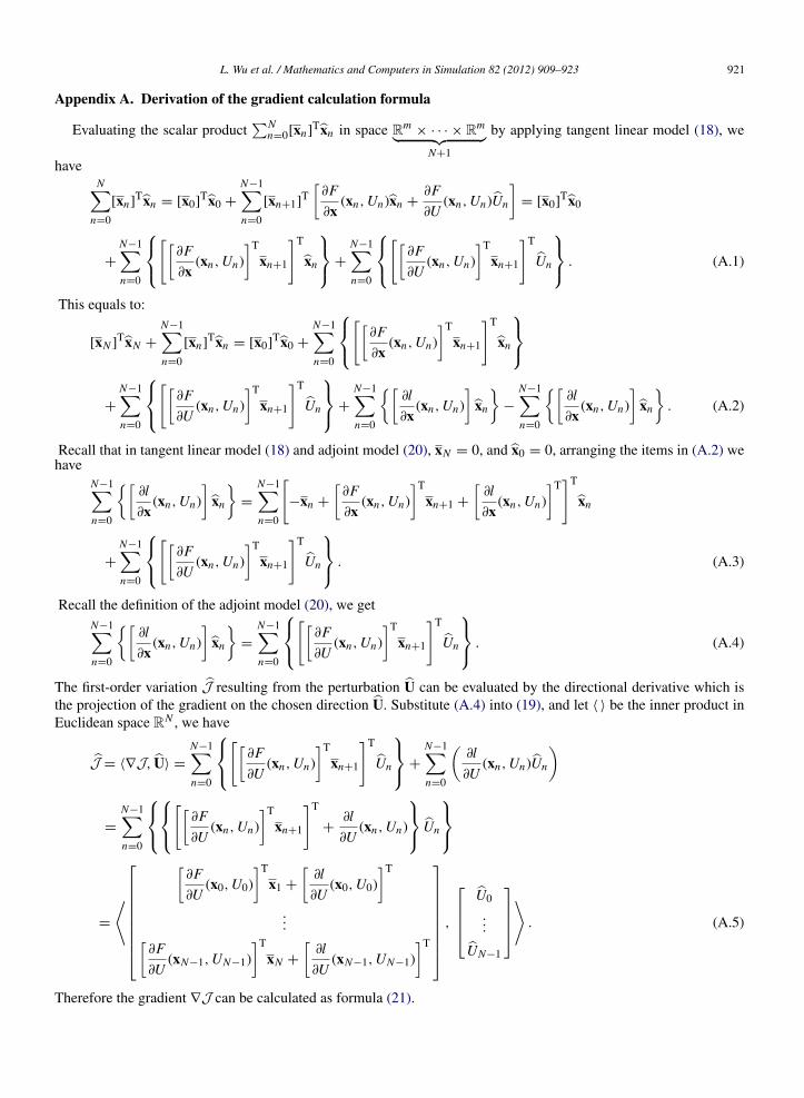
ppendix A. Derivation of the gradient calculation formula

Evaluating the scalar product∑N

n=0[xn]Txn in space Rm × · · · × R

m︸ ︷︷ ︸N+1

by applying tangent linear model (18), we

aveN∑

n=0

[xn]Txn = [x0]Tx0 +N−1∑n=0

[xn+1]T[∂F

∂x(xn, Un)xn + ∂F

∂U(xn, Un)Un

]= [x0]Tx0

+N−1∑n=0

⎧⎨⎩[[

∂F

∂x(xn, Un)

]T

xn+1

]T

xn

⎫⎬⎭+N−1∑n=0

⎧⎨⎩[[

∂F

∂U(xn, Un)

]T

xn+1

]T

Un

⎫⎬⎭ . (A.1)

This equals to:

[xN ]TxN +N−1∑n=0

[xn]Txn = [x0]Tx0 +N−1∑n=0

⎧⎨⎩[[

∂F

∂x(xn, Un)

]T

xn+1

]T

xn

⎫⎬⎭+

N−1∑n=0

⎧⎨⎩[[

∂F

∂U(xn, Un)

]T

xn+1

]T

Un

⎫⎬⎭+N−1∑n=0

{[∂l

∂x(xn, Un)

]xn

}−

N−1∑n=0

{[∂l

∂x(xn, Un)

]xn

}. (A.2)

Recall that in tangent linear model (18) and adjoint model (20), xN = 0, and x0 = 0, arranging the items in (A.2) weave

N−1∑n=0

{[∂l

∂x(xn, Un)

]xn

}=

N−1∑n=0

[−xn +

[∂F

∂x(xn, Un)

]T

xn+1 +[

∂l

∂x(xn, Un)

]T]T

xn

+N−1∑n=0

⎧⎨⎩[[

∂F

∂U(xn, Un)

]T

xn+1

]T

Un

⎫⎬⎭ . (A.3)

Recall the definition of the adjoint model (20), we getN−1∑n=0

{[∂l

∂x(xn, Un)

]xn

}=

N−1∑n=0

⎧⎨⎩[[

∂F

∂U(xn, Un)

]T

xn+1

]T

Un

⎫⎬⎭ . (A.4)

he first-order variation J resulting from the perturbation U can be evaluated by the directional derivative which ishe projection of the gradient on the chosen direction U. Substitute (A.4) into (19), and let 〈 〉 be the inner product inuclidean space R

N , we have

J = 〈∇J, U〉 =N−1∑n=0

⎧⎨⎩[[

∂F

∂U(xn, Un)

]T

xn+1

]T

Un

⎫⎬⎭+N−1∑n=0

(∂l

∂U(xn, Un)Un

)

=N−1∑n=0

⎧⎨⎩⎧⎨⎩[[

∂F

∂U(xn, Un)

]T

xn+1

]T

+ ∂l

∂U(xn, Un)

⎫⎬⎭ Un

⎫⎬⎭

=⟨⎡⎢⎢⎢⎢⎢⎢⎢

[∂F

∂U(x0, U0)

]T

x1 +[

∂l

∂U(x0, U0)

]T

...[ ]T [ ]T

⎤⎥⎥⎥⎥⎥⎥⎥ ,

⎡⎢⎢⎣U0

...

⎤⎥⎥⎦⟩

. (A.5)

⎣ ∂F

∂U(xN−1, UN−1) xN + ∂l

∂U(xN−1, UN−1)

⎦ UN−1

herefore the gradient ∇J can be calculated as formula (21).

[[[

[

[[

[

[

[[

[

[[

[

[

[

[[

[[

[

[

[

[

922 L. Wu et al. / Mathematics and Computers in Simulation 82 (2012) 909–923

References

[1] C. Bardos, O. Pironneau, Data assimilation for conservation laws, Methods Appl. Anal. 12 (2005) 103–134.[2] P. Boggs, J. Tolle, Sequential quadratic programming, Acta Numer. 4 (1995) 1–51.[3] J.F. Bonnans, J.C. Gilbert, C. Lemarechal, C.A. Sagastizábal, Numerical Optimization: Theoretical and Practical Aspects, second edition,

Springer, 2006.[4] C. Brouwer, H. Heibloem, Irrigation Water Management, Training Manuals – 3: Irrigation Water Needs, Food and Agriculture Organization

of the United Nations, 1986.[5] W. Chao, L.P. Chang, Development of a four-dimensional variational analysis system using the adjoint method at GLA. Part 1. Dynamics,

Mon. Weather Rev. 120 (1992) 1661–1673.[6] M. Chelle, Phylloclimate or the climate perceived by individual plant organs: What is it? how to model it? What for? New Phytol. 166 (2005)

781–790.[7] P.H. Cournède, M. Kang, A. Mathieu, J.F. Barczi, H. Yan, B.G. Hu, P. de Reffye, Structural factorization of plants to compute their functional

and architectural growth, Simul. Trans. Soc. Modell. Simul. Int. 82 (2006) 427–438.[8] E. Dayan, E. Presnov, M. Fuchs, Prediction and calculation of morphological characteristics and distribution of assimilates in the Rosgro model,

Math. Comput. Simul. 65 (2004) 101–116.[9] R. Giering, T. Kaminski, Recipes for adjoint code construction, ACM Trans. Math. Software 24 (1998) 437–474.10] P. Gill, W. Murray, M. Wright, Practical Optimization, Academy Press, 1981.11] A. Griewank, Evaluating Derivatives: Principles and Techniques of Algorithmic Differentiation, SIAM, Philadelphia, PA, 2000.12] Y. Guo, Y. Ma, Z. Zhan, B. Li, M. Dingkuhn, D. Luquet, P. de Reffye, Parameter optimization and field validation of the functional structural

model GREENLAB for maize, Ann. Bot. 97 (2006) 217–230.13] Y. Guo, P. de Reffye, Y.H. Song, Z.G. Zhan, M. Dingkuhn, B. Li, Modeling of biomass acquisition and partitioning in the architecture of

sunflower, in: B.G. Hu, M. Jaeger (Eds.), Plant Growth Modeling and Applications: Proceedings – PMA03, Tsinghua University Press andSpringer, Beijing, 2003, pp. 271–284.

14] F. Hallé, R. Oldeman, P. Tomlinson, Tropical Trees and Forests, Springer Verlag, Berlin, 1978.15] T.J. Howell, J.T. Musick, Relationship of dry matter production of field crops to water consumption, in: A. Perrier, C. Riou (Eds.), Proceedings

of the International Conference Les Besoins en Eau des Cultures, INRA, Paris, 1985, pp. 247–269.16] M. Kang, P.H. Cournède, P. de Reffye, D. Auclair, B.G. Hu, Analytical study of a stochastic plant growth model: application to the GreenLab

model, Math. Comput. Simul. 78 (2008) 57–75.17] W. Kurth, B. Sloboda, Growth grammars simulating trees—an extension of L-systems incorporating local variables and sensitivity, Silva Fenn.

31 (1997) 285–295.18] F.X. Le Dimet, H. Ngodock, B. Luong, J. Verron, Sensitivity analysis in variational data assimilation, J. Meteorol. Soc. Jpn. 75 (1997) 245–255.19] F.X. Le Dimet, O. Talagrand, Variational assimilation of meteorological observations: theoretical aspect, Tellus 38A (1986)

97–110.20] V. Letort, P. Mahe, P.H. Cournède, P. de Reffye, B. Courtois, Quantitative genetics and functional–structural plant growth models: sim-

ulation of quantitative trait loci detection for model parameters and application to potential yield optimization, Ann. Bot. 101 (2008)1243–1254.

21] J.L. Lions, Contrôle optimal de sysémes gouvernés par des équations aux dérivées partielles, Dunod: Gauthier-Villars, Paris, 1968.22] Y. Ma, B. Li, Z. Zhan, Y. Guo, D. Luquet, P. de Reffye, M. Dingkuhn, Parameter stability of the functional–structural plant model GREENLAB

as affected by variation within populations, among seasons and among growth stages, Ann. Bot. 99 (2007) 61–73.23] J.C. Mailhol, A.A. Olufayo, P. Ruelle, Sorghum and sunflower evapotranspiration and yield from simulated leaf area index, Agric. Water

Manage. 35 (1997) 167–182.24] L. Marcelis, E. Heuvelink, J. Goudriaan, Modelling biomass production and yield of horticultural crops: a review, Sci. Hortic. (Amsterdam)

(1998) 83–111.25] A. Mathieu, P.H. Cournède, D. Barthélémy, P. de Reffye, Rhythms and alternating patterns in plants as emergent properties of a model of

interaction between development and functioning, Ann. Bot. 101 (2008) 1233–1242.26] R. Mech, P. Prusinkiewicz, Visual models of plants interacting with their environment, Comput. Graph. 30 (1996) 397–410.27] J. Perttunen, R. Sievänen, E. Nikinmaa, H. Salminen, H. Saarenmaa, J. Väkevä, LIGNUM: a tree model based on simple structural units, Ann.

Bot. 77 (1996) 87–98.28] P. Prusinkiewicz, Modeling plant growth and development, Curr. Opin. Plant Biol. 7 (2004) 79–83.29] R. Qi, V. Letort, M. Kang, P.H. Cournède, P. de Reffye, T. Fourcaud, Application of the GreenLab model to simulate and optimize wood

production and tree stability: a theoretical study, Silva Fenn. 43 (2009) 465–487.30] F. Rabier, H. Järvinen, E. Klinker, J.F. Mahfouf, A. Simmons, The ECMWF operational implementation of four-dimensional variational

assimilation. I. Experimental results with simplified physics, Quart. J. Roy. Meteorol. Soc. 126 (2000) 1143–1170.31] P. de Reffye, F. Blaise, S. Chemouny, S. Jaffuel, T. Fourcaud, F. Houllier, Calibration of a hydraulic architecture-based growth model of cotton

plants, Agronomie 19 (1999) 265–280.32] P. de Reffye, C. Edelin, J. Francon, M. Jaeger, C. Puech, Plant models faithful to botanical structure and development, Comput. Graph. 22

(1988) 151–158.

33] P. de Reffye, T. Fourcaud, F. Blaise, D. Barthélémy, F. Houllier, A functional model of tree growth and tree architecture, Silva Fenn. 31 (1997)

297–311.

[

[

[

[

[

[

[

[

[

[

L. Wu et al. / Mathematics and Computers in Simulation 82 (2012) 909–923 923

34] R. Sievänen, E. Nikinmaa, P. Nygren, H. Ozier-Lafontaine, J. Perttunen, H. Hakula, Components of a functional–structural tree model, Ann.For. Sci. 57 (2000) 399–412.

35] O. Talagrand, The use of adjoint equations in numerical modelling of the atmospheric circulation, in: A. Griewank, G. Corliss (Eds.), AutomaticDifferentiation of Algorithms: Theory, Implementation, and Application, SIAM, 1991, pp. 169–180.

36] L. Wu, Variational methods applied to plant functional–structural dynamics: parameter identification, control, and data assimilation, Ph.D.thesis, Université Joseph Fourier, 2005.

37] L. Wu, V. Mallet, M. Bocquet, B. Sportisse, A comparison study of data assimilation algorithms for ozone forecasts, J. Geophys. Res. 113(2008) D20310.

38] L. Wu, P. de Reffye, B.G. Hu, F.X. Le Dimet, P.H. Cournède, A water supply optimization problem for plant growth based on GreenLab model,J. ARIMA (2005) 194–207.

39] H. Yan, M. Kang, P. de Reffye, M. Dingkuhn, A dynamic, architectural plant model simulating resource dependent growth, Ann. Bot. 93 (2004)591–602.

40] Z. Zhan, P. de Reffye, F. Houllier, B.G. Hu, Fitting a functional–structural growth model to plant architecture data, in: B.G. Hu, M. Jaeger(Eds.), Plant Growth Modeling and Applications: Proceedings – PMA03, Tsinghua University Press and Springer, Beijing, 2003, pp. 236–249.

41] J. Zhu, M. Kamachi, G. Zhou, Nonsmooth optimization approaches to VDA of models with on/off parameterizations: Theoretical issues, Adv.Atmos. Sci. 19 (2002) 405–424.

42] X. Zou, F. Vandenberghe, M. Pondeca, Y.H. Kuo, Introduction to adjoint techniques and the MM5 adjoint modeling system, Technical Report,

NCAR, 1997.

43] B.G. Hu, P. de Reffye, X. Zhao, H.P. Yan, M.Z. Kang, GreenLab: A new methodology towards plant functional-structual model-Structualaspect, in: B.G. Hu, M. Jaeger (Eds.), Plant Growth Modeling and Applications: Proceedings – PMA03, Tsinghua University Press andSpringer, Beijing, 2003, pp. 21–35.