An optimization-based model of theNordic power market

Caroline Tandberg

TIØ4500 - Specialization ProjectManagerial Economics and Operations ResearchSupervisor: Stein-Erik FletenDepartment of Industrial Engineering and Technology ManagementNorwegian University of Science and TechnologyDecember 14, 2011

2

Preface

This work has been done as a part of the subject TIØ4505 Managerial Economicsand Operations Research, Specialization Project at the Norwegian University ofScience and Technology (NTNU) during the autumn of 2011.

I would like thank my supervisor, Associate Professor Stein-Erik Fleten, for ad-vice and support during the report-writing. Special thanks also goes to ErlendTorgnes and Ole Lofsnes at Econ Pöyry for providing both data and guidancethroughout the semester.

i

ii

Abstract

In this paper, an optimization-based model of the Nordic power market is de-veloped. The objective of the proposed method is to minimize the total gener-ation cost, and the model is formulated as a deterministic linear program. Thedual values for the power balance constraints can be seen as the power price,and these power prices are forecasted in each of the Nordic countries for a two-year horizon. The model successfully allocates the different generating unitsand transmission lines according to the demand, minimizing the total systemcost during the planning horizon.

An important issue discussed in this paper is how to handle reservoirs in along-term perspective for a hydrothermal system. In the proposed method, thereservoirs are aggregated in the respective countries in addition to the inflowsbeing treated as deterministic parameters. This is a modeling oversimplifica-tion, and the results indicate that the power prices are very sensitive to a changein inflow-scenario. Other approaches to long-term hydrothermal schedulingwhere there is stochasticity involved are studied, and it is suggested that suchan approach will better suit reality.

iii

Contents

Preface i

Abstract iii

1 Introduction 11.1 The power system . . . . . . . . . . . . . . . . . . . . . . . . . . . . 1

1.1.1 Supply . . . . . . . . . . . . . . . . . . . . . . . . . . . . . . 11.1.2 Demand . . . . . . . . . . . . . . . . . . . . . . . . . . . . . 21.1.3 Deregulation . . . . . . . . . . . . . . . . . . . . . . . . . . 2

1.2 Generation planning . . . . . . . . . . . . . . . . . . . . . . . . . . 21.3 Hydropower as an energy source . . . . . . . . . . . . . . . . . . . 41.4 Structure of this report . . . . . . . . . . . . . . . . . . . . . . . . . 5

2 Related work 62.1 The development of stochastic solution methods . . . . . . . . . . 62.2 Dimensionality reduction approaches . . . . . . . . . . . . . . . . 62.3 Methods for the deregulated market . . . . . . . . . . . . . . . . . 7

3 Approaches to reservoir management 83.1 Dynamic programming . . . . . . . . . . . . . . . . . . . . . . . . 93.2 Stochastic dynamic programming . . . . . . . . . . . . . . . . . . . 11

3.2.1 The water value method . . . . . . . . . . . . . . . . . . . . 113.3 Approximate dynamic programming . . . . . . . . . . . . . . . . . 123.4 Stochastic dual dynamic programming . . . . . . . . . . . . . . . 13

4 Mathematical formulation 164.1 Sets and indices . . . . . . . . . . . . . . . . . . . . . . . . . . . . . 164.2 Parameters . . . . . . . . . . . . . . . . . . . . . . . . . . . . . . . . 174.3 Variables . . . . . . . . . . . . . . . . . . . . . . . . . . . . . . . . . 174.4 Data . . . . . . . . . . . . . . . . . . . . . . . . . . . . . . . . . . . . 18

4.4.1 Generation capacities . . . . . . . . . . . . . . . . . . . . . . 184.4.2 CHP generation . . . . . . . . . . . . . . . . . . . . . . . . . 184.4.3 Generation costs . . . . . . . . . . . . . . . . . . . . . . . . 194.4.4 Demand . . . . . . . . . . . . . . . . . . . . . . . . . . . . . 204.4.5 Transmission capacities . . . . . . . . . . . . . . . . . . . . 204.4.6 Reservoir data . . . . . . . . . . . . . . . . . . . . . . . . . . 214.4.7 Inflow . . . . . . . . . . . . . . . . . . . . . . . . . . . . . . 224.4.8 Outside region power prices . . . . . . . . . . . . . . . . . 22

4.5 Mathematical model . . . . . . . . . . . . . . . . . . . . . . . . . . 23

iv

4.6 Discussion of the model . . . . . . . . . . . . . . . . . . . . . . . . 244.6.1 Objective function . . . . . . . . . . . . . . . . . . . . . . . 244.6.2 Constraints . . . . . . . . . . . . . . . . . . . . . . . . . . . 24

4.7 Number of variables and constraints . . . . . . . . . . . . . . . . . 244.8 Implementation . . . . . . . . . . . . . . . . . . . . . . . . . . . . . 25

5 Results 265.1 Prices and costs . . . . . . . . . . . . . . . . . . . . . . . . . . . . . 26

5.1.1 Power balance . . . . . . . . . . . . . . . . . . . . . . . . . . 265.1.2 Water balance . . . . . . . . . . . . . . . . . . . . . . . . . . 265.1.3 Analysis . . . . . . . . . . . . . . . . . . . . . . . . . . . . . 30

5.2 Analysis of a single time period . . . . . . . . . . . . . . . . . . . . 315.3 Other inflow scenarios . . . . . . . . . . . . . . . . . . . . . . . . . 33

6 Conclusion and further work 376.1 Conclusion . . . . . . . . . . . . . . . . . . . . . . . . . . . . . . . . 376.2 Further work . . . . . . . . . . . . . . . . . . . . . . . . . . . . . . . 37

6.2.1 Improving the deterministic model . . . . . . . . . . . . . 376.2.2 Stochastic programming . . . . . . . . . . . . . . . . . . . . 38

Appendix A - Mosel code 41

v

List of Figures

1 Picture of the Nordic power market with connections to Europe(Source: Nord Pool) . . . . . . . . . . . . . . . . . . . . . . . . . . . . 3

2 Aggregated demand in the Nordics . . . . . . . . . . . . . . . . . . 203 Inflows in respective areas . . . . . . . . . . . . . . . . . . . . . . . 224 Power prices . . . . . . . . . . . . . . . . . . . . . . . . . . . . . . . 275 Water values . . . . . . . . . . . . . . . . . . . . . . . . . . . . . . . 286 Reservoir levels . . . . . . . . . . . . . . . . . . . . . . . . . . . . . 297 Power prices in case of high inflow . . . . . . . . . . . . . . . . . . 348 Power prices in case of low inflow . . . . . . . . . . . . . . . . . . 35

List of Tables

1 Generation capacities . . . . . . . . . . . . . . . . . . . . . . . . . . 182 Generator information . . . . . . . . . . . . . . . . . . . . . . . . . 193 Fuel characteristics . . . . . . . . . . . . . . . . . . . . . . . . . . . 194 Transmission capacities . . . . . . . . . . . . . . . . . . . . . . . . . 215 Reservoir data [GWh] . . . . . . . . . . . . . . . . . . . . . . . . . . 216 Generation costs . . . . . . . . . . . . . . . . . . . . . . . . . . . . . 317 Generation by type (average hourly production) . . . . . . . . . . 328 Shadow prices . . . . . . . . . . . . . . . . . . . . . . . . . . . . . . 329 Outside power prices [€/MWh] . . . . . . . . . . . . . . . . . . . . 3210 Border flow . . . . . . . . . . . . . . . . . . . . . . . . . . . . . . . 33

vi

1 Introduction

Operations research (OR) is currently used actively in power generation schedul-ing, and it is important that these tools are continuously improved. As comput-ers are getting better and power systems are expanding, there is much to gain byusing advanced optimization software to aid the decision-making process. Themain focus of this paper is long-term hydrothermal scheduling (LTHS), with anemphasis on the treatment of hydropower. The objective of the LTHS is to de-termine a generation schedule which minimizes the expected generation costsalong the planning period. Because there is a limited amount of water availablestored in reservoirs, the optimal operation is very complex. A system with agiven load and an endogenous price is considered, and the aim is to capturethe main properties of electricity prices through the model. While the Nordicpower system is the target area for investigation in this paper, the results areuniversally applicable, especially in other hydro-dominated systems.

1.1 The power system

In order to better understand the scheduling problem, it is important to grasphow a hydrothermal power system works. Electricity is generated and con-sumed continuously and simultaneously, and the role of the transmission sys-tem is to connect the location where the power is generated to substations lo-cated near consumers.

1.1.1 Supply

There are many forms of electricity generation, and they can be categorized intonuclear, thermal and renewable sources. Thermal sources run on fossil fuelssuch as coal and gas, and CO2 is released in the generation process. Renewablesources include hydro-, solar-, wind- and wave-power, and is characterized bythat the sources for it will never run out. These energy sources build the supplycurve according to their marginal costs, and in optimal system operation, thedemand is always covered with the cheapest possible combination of genera-tors.

1

1.1.2 Demand

Demand for power fluctuates during each 24-hour period and during each year.Since electricity is used for heating in most Scandinavian homes, the demandfor electricity is temperature dependent, and at its highest during the wintermonths. The demand can be predicted in the short-term with a very high ac-curacy according to daily load curves and forecasts. In the long-term however,there is a greater uncertainty about the load, and the load is usually dividedinto elastic and inelastic demand.

1.1.3 Deregulation

A trend in power markets show a move from regulated markets toward deregu-lated markets. In a deregulated market there is a separation between the poten-tially competitive functions of generation and retail from the natural monopolyfunctions of transmission and distribution. Introduction of a deregulated mar-ket in the Nordics came in the beginning of the 90s, and there is now com-petition between the different power producers. The objective of the powerproduction scheduling has therefore gone from a cost minimization to a profitmaximization objective. In a liberalized market there is no effect of these differ-ent objectives, because they result in the same production plans. A liberalizedmarket requires that a large number of buyers can buy from a large number ofsuppliers or producers. Nord Pool is the Nordic power exchange and selects thebids so that welfare is maximized (Wangensteen, 2007). Figure 1 shows a mapof the Nordic region with the physical transmission lines and the price areasused by Nord Pool.

1.2 Generation planning

The task of planning the power generation is complicated by the presence ofuncertainties. In the future very little is known for sure, and there is uncer-tainty associated with many factors, the most important being; inflows, powerprices, consumption, fuel costs and CO2 prices. In Norway most of the elec-tricity generation comes from hydropower, but because of the connections tothe continent, a hydrothermal system must be modeled. Seen from a socio-economic point of view, the objective of optimal operation of such a systemis to determine a strategy which, for each stage in the planning period, giventhe system state, produces generation targets for each plant that will minimizethe expected value of generation costs. These costs consists of fuel costs for

2

Figure 1: Picture of the Nordic power market with connections to Europe(Source: Nord Pool)

thermal units, purchase costs from neighboring systems, plus the penalties forfailure of load supply. Everything ranging from generation, transmission andreservoir levels must be decided, and the ideal solution would be one single op-timization process, taking into account everything and resulting in the optimalsolution. However, due to the span in space and time, this is impossible to dowith the required level of detail. The result is that the scheduling is divided intothree stages; long-, medium-, and short-term.

From the long-term scheduling, a price forecast for the next 1-5 years is found.Although the time horizon can be much longer, up to 20-30 years, the definitionof LTHS in this report is 1-5 years. The inputs into the model is everything fromgeneration capacities in the different areas to demand forecasts. The areas usedcan be the same as the Nord Pool areas, or they could be even more detailed

3

and based on river systems and bottlenecks. The main goal of the long-termscheduling is to find out how the water resource should be used during thewhole period, and for hydro-producers this serves as strategic management.This is important to find out since there is only a limited amount of water, andthis amount available is not known exactly due to uncertain inflows. Examplesof models used for this purpose includes ECON BID and the EMPS model. Inthese models, the Nordic system is divided into a number of areas, and thereservoirs in each area is aggregated. The uncertainty of inflow is taken intoaccount.

The seasonal scheduling serves as a link between the long-term and the short-term scheduling. The time horizon ranges from 3 - 18 months, and the modeluses a simplified representation of uncertainty, and can even be deterministic.The main goal is to optimize the use of water within the period, while the endof the modeling period values must match with the corresponding long-termvalues. These values are can be either water values or reservoir levels, depend-ing on how the models are coupled. The seasonal scheduling includes a moredetailed representation of the system, and water values for the individual reser-voirs are calculated. Water values are explained further in Section 3.2.1

In the short-term scheduling, a deterministic model is used where inflow andand prices are assumed known. A detailed description of the system is used,and a unit commitment problem is solved where the number and type of gen-erators in use are decided.

1.3 Hydropower as an energy source

The combination of very high mountains and large plains in the Nordics makeperfect conditions for reservoir-building. Collecting millions of tons of waterin huge dams provides a means for controlling both the timing and the scale ofhydro-generation. Many of the large reservoirs in Norway are situated in placeswhere precipitation falls as snow during the winter, and this means low inflowinto the reservoirs during winter. A snow reservoir builds up in the mountains,and when this starts to melt in spring, the inflow into the reservoirs is high. Themelting season can continue well into the summer months.

Reservoirs provide a means for storing energy, and from an operations researchpoint of view there are many decisions that must be made so that the reservoiris used in an optimal way depending on what goals one is pursuing. Reservoirscan be modeled mathematically and a set of assumptions, constraints, objectivesand decision variables are specified. There are many factors which complicate

4

the operational decisions of a hydro-plant owner, and the model should striveto include these factors. The most important complications are given in thissection.

For hydro plants, a discharge capacity in m3/s and an energy equivalent e inkWh/m3 is usually specified (Doorman, 2009):

e =1

3.6× 106 ·γgHη [kWh/m3] (1.1)

where

γ : water density [kg/m3]g : gravity acceleration [m/s2]H : plant head [m]η : plant efficiency

In reality, the efficiency of the plant η will depend on the discharge and theplant head. This results in a nonlinear relation between turbine discharge andpower output. In the EMPS model, this is represented by a piecewise linearcurve. In other models, a linear relationship is assumed in order to simplifythe model. When reservoirs are aggregated and one large reservoir is modeled,assumptions of constant efficiency is usually accepted. However in short-termscheduling, this nonlinearity has a larger effect due to larger variations in head,and should be taken into account for the plant efficiency η.

Reservoirs are usually hydraulically coupled with other reservoirs, and largeriver systems should be modeled. If aggregation is used in the model, disaggre-gation methods are applied in order to get a feasible solution. Heuristics can beused for this purpose, although optimality can not be guaranteed.

1.4 Structure of this report

In the next section relevant literature is presented. Section 3 gives an overviewof the approaches developed for long-term hydrothermal scheduling. The meth-ods presented are deterministic and stochastic, and the strengths and weak-nesses of each mettod is discussed. In Section 4, an example of a deterministiclinear program is described. This model and the results are then analyzed andevaluated in Section 5, and the final conclusions and future work are given inSection 6.

5

2 Related work

In this section, related work regarding reservoir handling and hydrothermalscheduling is reviewed. Yeh (1985) classified the methods available for opti-mal reservoir handling at the time into four categories; linear programming(LP), dynamic programming, nonlinear optimization and simulation. Severalof these methods can be combined in different ways, but few models deal si-multaneously with all the aspects of the scheduling problem such as multipleperiods, multiple reservoirs and stochastic inflows.

2.1 The development of stochastic solution methods

One common simplification is to use a deterministic model by replacing stochas-tic components by their expected values as in Soares and Carneiro (1991). It wasimplied early on by Massé (1946), and later argued by Gjelsvik (1982), that de-terministic models are not well suited for the planning problem as they are notflexible enough. Stochastic dynamic programming and dynamic programminghas been used in the scheduling problem for a long time, an early reference be-ing Buras (1963). Yakowitz (1982) reviews the evolution of these models, andof these papers Turgeon (1980) is of particular importance. It aims to developa method that deals with multi-reservoir systems by breaking up the originalproblem into a series of subproblems that are solved by dynamic programing.Egeland et al. (1982) is another example where decomposition methods are usedto solve the multi-reservoir problem. In Gjelsvik et al. (1992) some stochasticmethods are reviewed together with some important applications. A more re-cent review of dynamic programming applied to reservoir operation is givenin Nandalal and Bogárdi (2007). In Wolfgang et al. (2009) an application ofstochastic dynamic programming called the water value method is explainedin relation to the EMPS model. The reservoirs are aggregated and heuristicsare used in the de-aggregation procedure. Early investigations into the wa-ter value approach can be found in Stage and Larsson (1961) and in Lindqvist(1962).

2.2 Dimensionality reduction approaches

Because the dimensionality of stochastic dynamic programming can quickly getvery large due to the curse of dimensionality, it has limited use for real-worldproblems. Birge (1985) develops decomposition and partitioning methods that

6

are able to handle multidimensional problems, and these methods are furtherdeveloped and applied to the generation scheduling problem by Pereira andPinto (1985). This method is called stochastic dynamic dual programming, andwas successfully applied to a 37-reservoir system, although larger systems havebeen solved more recently. Ferrero et al. (1998) aims at reducing the dimen-sionality of dynamic programming by limiting the time period to a two-stagealgorithm that can handle multiple reservoirs.

2.3 Methods for the deregulated market

Yu et al. (1998) proposes a method that maximizes profit for hydroelectric plantsin a deregulated system. The method breaks down the long-term problem intomonthly based mid-term problems without using an exact cost function. Mar-ket power of producers in a deregulated market is discussed in Scott and Read(1996), where a multistage programming algorithm is employed called the dualdynamic programming. Their focus is in the New Zealand market where thereare relative few suppliers, and each sub-problem is solved using a Cournotduopoly model. An evaluation of the efficiency of the Nordic market is per-formed by Halseth (1999), where a special case of supply curve equilibrium isused to describe possible strategies for suppliers.

7

3 Approaches to reservoir management

Reservoirs used for power generation should be managed in such a way thatis optimal, and as discussed in the introduction, an optimal solution is one thatminimizes operational costs of generation. Each single company must decideon how much water should be stored and how much should be released forgeneration in all periods. There are many factors that makes this a very difficulttask (Soares and Carneiro, 1991):

• Long horizon of analysis (usually 2-3 years, but in reality to infinity)

• Stochastic nature of water inflows and load

• Operational inter-dependence between hydro plants in the same cascade

• Nonlinearity of thermal costs and hydro generation function.

In order to make the LTHS problem easier to solve, many simplifications canbe done. Deterministic models assume that future inflows and demands areknown along the planning period. Inflows can for example be replaced bytheir expected values. Linear Programming (LP) models linearize the nonlin-ear cost functions and hydro generation functions. In LP-models, the reservoirsare measured in MWh, and each unit of water has an energy equivalent value.Constant marginal cost is assumed for the thermal generators. Another simplifi-cation that is done in order to avoid the hydraulic coupling between reservoirs,is to aggregate the reservoirs into one large reservoir in each area. A simpledeterministic, one-area, LP-model is given here for reference:

minW = ∑t∈T

[∑

g∈GCgtxgt

]subject to:

∑g∈G

xigt = Dt ∀t ∈ T (3.1)

yt+1 − yt + xhydro,t ≤ It ∀t ∈ T (3.2)

yMin ≤ yt ≤ yMax ∀t ∈ T (3.3)

∑g∈G

xgt ≤ GCg ∀g ∈ G, ∀t ∈ T (3.4)

8

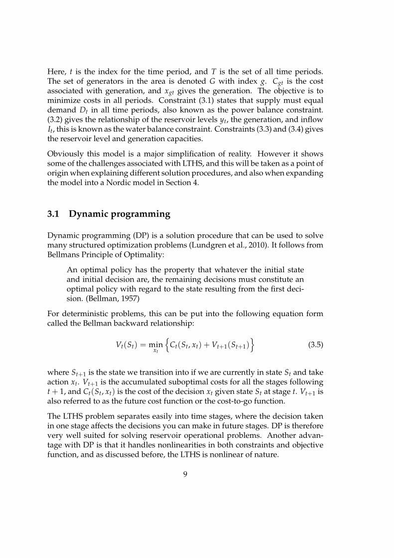
Here, t is the index for the time period, and T is the set of all time periods.The set of generators in the area is denoted G with index g. Cgt is the costassociated with generation, and xgt gives the generation. The objective is tominimize costs in all periods. Constraint (3.1) states that supply must equaldemand Dt in all time periods, also known as the power balance constraint.(3.2) gives the relationship of the reservoir levels yt, the generation, and inflowIt, this is known as the water balance constraint. Constraints (3.3) and (3.4) givesthe reservoir level and generation capacities.

Obviously this model is a major simplification of reality. However it showssome of the challenges associated with LTHS, and this will be taken as a point oforigin when explaining different solution procedures, and also when expandingthe model into a Nordic model in Section 4.

3.1 Dynamic programming

Dynamic programming (DP) is a solution procedure that can be used to solvemany structured optimization problems (Lundgren et al., 2010). It follows fromBellmans Principle of Optimality:

An optimal policy has the property that whatever the initial stateand initial decision are, the remaining decisions must constitute anoptimal policy with regard to the state resulting from the first deci-sion. (Bellman, 1957)

For deterministic problems, this can be put into the following equation formcalled the Bellman backward relationship:

Vt(St) = minxt

Ct(St, xt) + Vt+1(St+1)

(3.5)

where St+1 is the state we transition into if we are currently in state St and takeaction xt. Vt+1 is the accumulated suboptimal costs for all the stages followingt + 1, and Ct(St, xt) is the cost of the decision xt given state St at stage t. Vt+1 isalso referred to as the future cost function or the cost-to-go function.

The LTHS problem separates easily into time stages, where the decision takenin one stage affects the decisions you can make in future stages. DP is thereforevery well suited for solving reservoir operational problems. Another advan-tage with DP is that it handles nonlinearities in both constraints and objectivefunction, and as discussed before, the LTHS is nonlinear of nature.

9

The elements of dynamic programming, together with the implications for op-timal reservoir handling, are as follows (Powell, 2007):

The state variable This captures all the information we need to make adecision, as well as the information we need to describe how the systemevolves over time. In our case the state variable is the reservoir level,St = yt. In the multiple reservoir case this will be a vector containing allthe reservoir levels, St = (y1t, ..., ynt), where n is the number ofreservoirs.

The decision variable Decisions represent how we control the process. In thecase of LTHS the decision in each stage is how much water to releasefrom the reservoir for power generation, xhydro,t. It also involves decidinghow much thermal power to produce.

Exogenous information This is data that first becomes known each timeperiod, which in our case is the inflow into each reservoir, It.

The transition function This function determines how the system evolvesfrom the state St to the state St+1 given the decisions that was made attime t and the new information that arrived between t and t + 1. This isthe physical relationship between the reservoir level in t + 1 and t, whichis equation (3.2) above.

The contribution function This determines the costs incurred or the rewardsreceived during each time interval, ie. the cost of producing x amount ofenergy in period t.

The objective function Here we formally state the problem of minimizing thecost over a specified time period. The minimization is subjected toconstraints in storage volume and release.

The solution process starts at the final stage T where the cost VT(ST) is sup-posed to be known. In this way, it is possible to work backwards and find theoptimal decisions at every stage and state. Decision tables providing optimalwater discharge and operational costs for each possible discrete state of the sys-tem are given by this procedure. By using Bellman’s principle and workingbackwards in time using the fact that the optimal decisions are known in thefuture states, the number of decision variables are radically reduced.

In DP, the states must be discretized. That means that at each stage the reser-voir levels are evaluated across a range of possible levels. The problem becomesmore realistic the more reservoir levels one operates with. However the prob-lem also becomes very large, especially when the state variable is a vector (in

10

the multiple-reservoir case). This is known as the "curse of dimensionality" andprohibits large problems from being solved using DP.

3.2 Stochastic dynamic programming

Uncertainty is an important factor in reservoir management. There is uncer-tainty in all the factors discussed in Section 1.2, but our focus here will be onstochastic nature of inflow. In Stochastic dynamic programming (SDP), thepresent decision is optimized with this uncertainty taken into account. A prob-ability distribution of possible inflow scenarios is considered in each stage, anda multi-stage stochastic optimization is performed for each possible outcome.The SDP optimization process derives the optimal operating strategy from Bell-man’s backward recursive relationship (given here for a single reservoir optimaloperation) (Nandalal and Bogárdi, 2007):

Vt(St) = minxt

Ct(St, xt) + EVt+1(St+1)

(3.6)

The objective is to minimize the expected sum of costs over the whole timeperiod. The difference between SDP and DP is that SDP takes stochasticity intoaccount.

3.2.1 The water value method

The water value method is a special version of SDP, and can be used to solvethe LTHS problem (Wolfgang et al., 2009). The more water that is used for gen-eration in the present period reduces the availability of water in the future. Thevalue of using water in the present period must therefore be balanced againstthe possibility of using that water in the future. The value of the water is afunction of future development depending on load, inflow and market prices.The "water value", which is actually the expected marginal value of the energystored in the reservoir, is calculated at each decision stage. These are calculatedrecursively, starting at the end of the period. Some starting values for the lasttime period, T, must be used in order to be able to calculate the water values intime period T − 1. These are usually estimated. The more water the reservoirhas, the less the value of the water will be. The water values at stage T − 1 isthen found by finding the optimal operation of the reservoir considering theinflow probabilities and the water values in period T. One can calculate thewater values recursively, and in the end a table with water values at all stages

11

and reservoir levels has been found. These can then be used to help to find theoptimal decisions in the current stage.

Both DP and SDP have the disadvantage of having to discretize all the futurestates. The expected cost is calculated at each possible state, and this in turncauses the problem to grow exponentially in size when more variables andstates are added. Although they handle nonlinearities very well, the curse ofdimensionality limits their use. Aggregation of reservoirs is a method used tolower the number of variables needed, but the dimensionality of the problem isstill very large. The use of SDP is usually limited to handling only a handful ofreservoirs. (Gjelsvik et al., 1992)

3.3 Approximate dynamic programming

Approximate dynamic programming (ADP) is similar to DP, but instead of thebackward recursive relationship, the solution procedure steps forward throughtime. In DP, the solution requires that we loop over all possible states, exactlycomputing the value function which we then use to produce optimal decisions.In ADP, the future value function is not known, and hence it cannot use thealgorithm for DP. The value function is instead approximated in an iterativemanner for all possible states. In each iteration only some of the value functionsare updated.

Moving forward in time, the exogenous information is estimated in each stage,and a sample path is followed. In the LTHS problem this sample path representsa unique sequence of inflows, and these can be estimated by using the proba-blitity distribution together with a Monte Carlo simulation.

Once we have the approximated value functions Vt(St) and the sample path,optimal decisions can be taken moving forward through the sample path. Aftereach iteration a new sample path is made, and the approximated value func-tions in iteration n, are improved by using to the following equation:

vnt = min

xt∈χnt

Ct(Sn

t , xt) + γ ∑ω∈Ωn

t+1

pt+1(ω)Vn−1t+1 (St+1)

(3.7)

The improved approximated value function, Vnt , is then computed by using a

weighting between vnt and Vn−1

t , known as "smoothing". This equation is simi-lar to the backward recursive equation of DP, but the expected value function is

12

replaced by its approximation Vn−1t+1 (St+1) that was found in the previous itera-

tion. χnt is the feasible region for the decisions xt, Ωn

t+1 are all the possible sets ofoutcomes in the inflow, while pt+1(ω) is the probability of outcome ω ∈ Ωn

t+1.γ ≤ 1 is a discount factor.

In ADP, there is no need to loop over all possible states, and there is also no re-quirement that the inflow scenarios are independent from the previous period.However there are a few downsides with ADP that has to be dealt with; Weonly update the values of states we visit, but the states we have not visited getsthe same value as in the last iteration. This can eventually cause these states tolook uninviting even though they can produce better value functions. There isstill a need to find the set of possible inflows, and the states of the system needsto be discretized.

3.4 Stochastic dual dynamic programming

Stochastic Dual Dynamic Programming (SDDP) is a very powerful method tosolve the hydrothermal problem without the need for discretization of futurestates. It is described in Pereira and Pinto (1991), and it is able to handle multi-reservoir systems. SDDP is based on approximation of the expected cost-to-gofunction of SDP by piecewise linear functions. These piecewise functions areobtained from the dual values of the optimization problem.

We first study a two-stage, one-reservoir deterministic example. This is equiva-lent to a Benders decomposition algorithm (Benders, 1962), which can be statedas follows:

minx,y

w = f (x) + cT y (3.8)

s.t. Ay + Bx ≥ I (3.9)

This problem can be regarded as a general form of the reservoir optimizationproblem where x is the discharge decision taken here and now, and cT y is thefuture cost function at reservoir level y. The constraint (3.9) is a general formof the water balance constraint (3.2). The other constraints are left out herefor simplicity. For a given discharge decision x, the second stage problem willbe:

13

minα = cT y (3.10)s.t. Ay ≥ I − Bx (3.11)

And the first-stage optimization problem is:

min w = f (x) +α(x) (3.12)

By taking the dual of the second-stage problem we get a maximization prob-lem:

max π(I − Bx) (3.13)s.t. ATπ ≤ c (3.14)

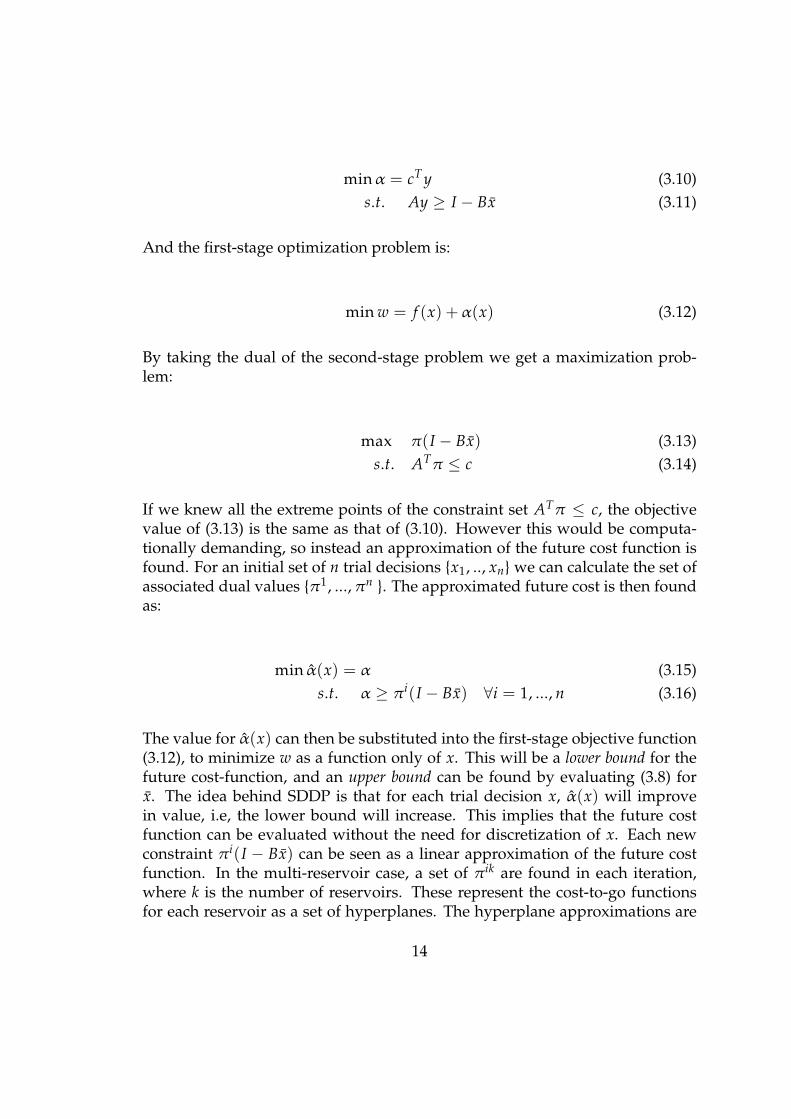
If we knew all the extreme points of the constraint set ATπ ≤ c, the objectivevalue of (3.13) is the same as that of (3.10). However this would be computa-tionally demanding, so instead an approximation of the future cost function isfound. For an initial set of n trial decisions x1, .., xn we can calculate the set ofassociated dual values π1, ..., πn . The approximated future cost is then foundas:

min α(x) = α (3.15)s.t. α ≥ π i(I − Bx) ∀i = 1, ..., n (3.16)

The value for α(x) can then be substituted into the first-stage objective function(3.12), to minimize w as a function only of x. This will be a lower bound for thefuture cost-function, and an upper bound can be found by evaluating (3.8) forx. The idea behind SDDP is that for each trial decision x, α(x) will improvein value, i.e, the lower bound will increase. This implies that the future costfunction can be evaluated without the need for discretization of x. Each newconstraint π i(I − Bx) can be seen as a linear approximation of the future costfunction. In the multi-reservoir case, a set of π ik are found in each iteration,where k is the number of reservoirs. These represent the cost-to-go functionsfor each reservoir as a set of hyperplanes. The hyperplane approximations are

14

built iteratively, to give increasing accuracy. By choosing the initial dischargedecisions with care, we can quickly get a very good representation of the futurecost-to-go function. In this way, the many-dimensional water value tables usedin SDP are avoided.

Extensions to this model are used to represent the multistage, stochastic prob-lems. For the multistage problem with T time periods, the algorithm runs it-eratively forwards and backwards through all the time periods. In the forwardrun, the optimization problem is solved with a set of trial decisions xt−1 forevery stage t. In the backward run, additional hyperplanes are constructed inthe previous stage by using multipliers found in the current stage. To extendthe problem into the stochastic one, we assume that the inflow vector It is dis-cretized into m scenarios It j, j = 1, ..., m. The idea is then to determine "good"trial decisions at each stage. Ideally the forward and backward iteration is runfor every combination of scenarios It j, but more realistically, a Monte Carlo sim-ulation is carried out.

15

4 Mathematical formulation

An outline of a deterministic LP model that can be used to solve the LTHS isgiven in this section. It is an extension of the model outlined in the start of Sec-tion 3, and the goal of the model is to forecast the spot price in each country ofthe Nordic region. The countries consists of Norway (NO), Sweden (SE), Fin-land (FI) and Denmark (DK). The outside world has been modeled according totheir power prices, and the most important countries to model is the exchangewith Germany (GE), Poland (PO) and the Netherlands (NL). The data used inthe model together with sources are given in Section 4.4, while the mathematicalmodel is given in Section 4.5.

4.1 Sets and indices

A : set of areas, indexed by i :T : set of time periods, indexed by t :L : set of transmission lines, indexed by l :F : set of fuel types, indexed by f :G : set of generator types, indexed by g :K : set of generator categories, indexed by k :J : set of outside regions, indexed by j :

16

4.2 Parameters

α : curtailment cost (constant)γ : losses in the lines in percentCgt : running cost of generator type g in time period t (€/MWh)Dit : firm demand in area i in period tTCl : transmission capacity of flow in line l (MWh/h)GCki : capacity of generator type k in area i (MW)CHPt : CHP generation in time period t (MWh/h)Iit : inflow in area i in period t (MWh/h)yMax

i : reservoir maximum in area iyMin

i : reservoir maximum in area iyStart

i : start reservoir level in area iyEnd

i : end reservoir level in area iToAl : gives the area/region that line l goes toFrAl : gives the area/region that line l goes fromPPjt : power prices in outside region j in time period tPFf t : fuel prices of fuel type f in time period tPCt : price of CO2-quota in time period tN f : carbon content in fueltype fE f : energy content in fueltype fVg : variable operating cost of generator type g tηg : efficiency of generator gGcatg : gives the generator category of generator type g

4.3 Variables

xigt : generation of generator type g in area i in time period tyit : reservoir level in area i in beginning of time period tzit : curtailment in area i in period tblt : cross border flow in transmission line l period t

17

4.4 Data

The granularity of the model is hourly, and the time horizon is two years. Datafor the model is from the years 2008 and 2009, and these are the years to beforecasted. The data that is too large to present here can be found in the file"data.xls".

4.4.1 Generation capacities

Generation capacities are assumed to be constant for the whole of the modelingperiod. Capacities are given for hydro, nuclear, thermal and gas turbines in eacharea. The category "thermal" consists of a few generator types that are groupedinto one category. The capacities can be seen in Table 1, and the data is fromNordel.

Table 1: Generation capacities

NO SE FI DKHydro 29474 16195 3097 0Nuclear 0 8938 2646 0Thermal 0 2271 2935 784Gasturbine 699 1607 840 412

Wind generation is stochastic and is left out of the model due to lack of hourlydata. The curtailment cost is constant and equal to 1000 €/MWh.

4.4.2 CHP generation

Combined heat and power (CHP) units can produce both heat and electricalpower, and is divided into Industry and District generation. The power gener-ation depends on both fuel prices and outside temperature. As a simplification,CHP is modeled as a fixed generation profile, i.e. one that is not optimized onthe basis of prices. The data is from Finnish Energy Industry, Svensk Energiand Energinet, and is the combined production from CHP Industry and CHPDistrict. The hourly production is simulated from the weekly generation.

18

4.4.3 Generation costs

The following equation was used to calculate the running cost of the generatortypes in all time periods:

Cgt =PFf t

E fηg+ Vg +

PCtN f

ηg(4.1)

The cost of generation depends on the cost of the fuel used, the variable cost ofproduction, and the CO2 quota prices. The efficiency of a generator type is alsorelevant for generation costs, and a table containing important characteristicsfor the different generator types can be found in Table 2. The fuel types used inthe model are coal and gas, and the hourly fuel prices are derived from weeklyaverage prices. While the data for the gas prices are from Nord Pool Gas, thecoal prices are from Vattenfall. Oil prices have minimal effect on the generationcosts as there are few generators running on oil in the Nordics. Therefore oilprices are not included in this model. The CO2 quota prices only change oncedaily, but in the model they are specified hourly. The quota prices are also fromVattenfall. Data for carbon and energy content for each fuel type is presented inTable 3. The data in Tables 2 and 3 are from Econ Pöyry.

Table 2: Generator information

Generator type Category Fuel type Efficiency Variable Cost[€/MWh]

CoalCondensing Thermal Coal 42 % 1.5CoalExtraction Thermal Coal 41 % 1.5GasExtraction Thermal Gas 39 % 1.5CCGT Thermal Gas 54 % 0.8GasTurbine Gasturbine Gas 38 % 0.8Hydro Hydro Water 100 % 0Nuclear Nuclear Uranium 100 % 15

Table 3: Fuel characteristics

Fuel type Carbon content Energy content[ton/MWh] [MWh/ton]

Coal 0.34 7.17Gas 0.20 13.33

19

4.4.4 Demand

The hourly demand in each area is found from the aggregated demand togetherwith the daily demand distribution between the areas. The demand distributionis assumed constant throughout the day, hence we can calculate the hourly de-mand in each area. The daily consumption data is from Nord Pool, and the totalhourly demand is from Vattenfall.

Figure 2: Aggregated demand in the Nordics

In Figure 2, it can be seen how the demand for power fluctuates during the year,and there are also major daily variations.

4.4.5 Transmission capacities

Transmission capacities between regions are found by aggregating area-capacitiesto a country level. The transmission capacities are modeled as constant through-out the entire period, and they can be seen in Table 4. The data is from EconPöyry. Losses are assumed to be 1% of the transmitted amount.

20

Table 4: Transmission capacities

From area To area Capacity [MW]NO SE 3550NO DK 950NO FI 100SE NO 3900SE DK 1980SE FI 2050DK NO 950DK SE 2440FI NO 100FI SE 1650NO NL 700SE GE 600SE PO 600DK GE 2085GE SE 600GE DK 1550NL NO 700PO SE 600

4.4.6 Reservoir data

The reservoir capacities in GWh are aggregated for each area as if there wasone large reservoir in each country. The starting level in each country is given,and the final reservoir level is not allowed to be smaller than a certain amount.The data is given in Table 5, and is from NVE, Svensk Energi and Finnish en-vironment inst. The minimum reservoir level in all periods is 1000 GWh in allcountries.

Table 5: Reservoir data [GWh]

Norway Sweden FinlandReservoir capacity 81888 33758 5530Start value 60901 23587 4113End value 55342 19636 3155

21

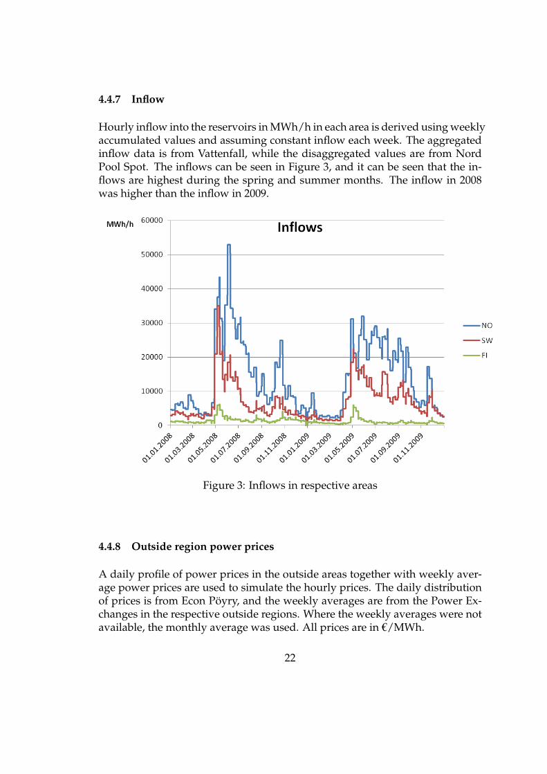
4.4.7 Inflow

Hourly inflow into the reservoirs in MWh/h in each area is derived using weeklyaccumulated values and assuming constant inflow each week. The aggregatedinflow data is from Vattenfall, while the disaggregated values are from NordPool Spot. The inflows can be seen in Figure 3, and it can be seen that the in-flows are highest during the spring and summer months. The inflow in 2008was higher than the inflow in 2009.

Figure 3: Inflows in respective areas

4.4.8 Outside region power prices

A daily profile of power prices in the outside areas together with weekly aver-age power prices are used to simulate the hourly prices. The daily distributionof prices is from Econ Pöyry, and the weekly averages are from the Power Ex-changes in the respective outside regions. Where the weekly averages were notavailable, the monthly average was used. All prices are in €/MWh.

22

4.5 Mathematical model

minW = ∑t∈T

[∑i∈A

∑g∈G

Cgtxigt (4.2a)

+ ∑i∈Aαzit (4.2b)

+ ∑j∈J

(∑

l∈L|ToAl= jPPjtblt − ∑

l∈L|FrAl= jPPjtblt

)](4.2c)

subject to

∑g∈G

xigt + zit + ∑l∈L|ToAl=i

blt − ∑l∈L|FrAl=i

blt = Dit − CHPt (4.3)

∀i ∈ A, ∀t ∈ T

yi,1 = yStarti (4.4)

∀i ∈ A

yi,t+1 − yit + xi,hydro,t ≤ Iit (4.5)∀i ∈ A, ∀t ∈ T

yMini ≤ yit ≤ yMax

i (4.6)∀i ∈ A, ∀t ∈ T

yi,nT ≥ yEndi (4.7)

∀i ∈ A

∑g∈G|Gcatg=k

xigt ≤ GCki (4.8)

∀i ∈ A, ∀k ∈ K, ∀t ∈ T

blt ≤ TCl (4.9)∀l ∈ L, t ∈ T

23

4.6 Discussion of the model

4.6.1 Objective function

The objective is to minimize total cost in all areas and time periods, and theseconsists of generation cost (4.2a) and curtailment costs (4.2b). In addition thereis the possibility to trade power with the outside regions. This is represented inthe objective function as a negative cost when selling and a positive cost whenbuying as seen in the part (4.2c).

4.6.2 Constraints

Constraint number (4.3) is the power balance constraint, making sure the de-mand is covered in all areas and time periods. The demand is either coveredby their own generation, by import/export, or by demand curtailment. The zitfunctions as a slack variable, and an alternative to having such a slack variablewith a high cost is to change the equality sign with a greater than or equalto sign. Then the problem would be infeasible if the system was unable tocover the demand, so the current formulation provides a greater flexibility. Con-straints (4.4), (4.6) and (4.7) are reservoir constraints on the minimum and max-imum level of water and the start and end values. (4.5) is the reservoir balanceconstraint giving the link between inflow, hydro generation and the reservoirlevels. A spill variable could have been used here to give equality, but it is notnecessary in this formulation as we have a maximum reservoir level. (4.8) givesthe capacity constraint of each generator category in each period and area, while(4.9) gives the transmission capacity constraint for each line in all periods.

4.7 Number of variables and constraints

If all the variables are created, the number of variables would be:

|A| × |G| × |T|+ |A| × |T|+ |A| × |T|+ |L| × |T|

And the number of constraints:

|A| × |T|+ |A|+ |A| × |T|+ |A| × |T|+ |A|+ |A| × |K| × |T|+ |L| × |T|

24

With |T| =17544 time periods, |G| =7 generator types, |A| =4 areas and |L| =18transmission lines, the number of variables is 947 373 and the number of con-straints are 807 024. However we know that some of the variables will not takeany values so we can choose not to create these variables. For example there areno reservoirs in Denmark, to the yit-variables for denmark do not need to becreated. In XpressMP, this is done by creating the variables dynamically as weneed them. By doing this, the number of variables is reduced to 877 197. This isstill a large number of variables, and the solution time is 270 seconds.

By having an hourly resolution in the model the number of variables is verylarge. In a deterministic model it is solvable, but in stochastic models the num-ber of variables created would be very large. It is therefore common to havea larger time resolution for stochastic models, for example weekly or monthly.The challenge is then to secure load capacity for peak load. This is done by us-ing a load curve that shows the distribution of power consumption during thetime period.

4.8 Implementation

The solver package used is XpressMP and the implementation is written in theMOSEL language. The optimizer solves the model with the data presented inSection 4.4 with regards to the constraints and objective presented in Section4.5. The MOSEL-code is attached in Appendix A.

25

5 Results

Results from running the model is given in this section together with someanalysis of these results. In Section 5.1, power prices, water values and reser-voir levels are discussed. In Section 5.2, a glimpse of what is happening in agiven time period is analyzed, while in Section 5.3 other inflow scenarios arediscussed.

5.1 Prices and costs

In optimization, the dual value of the constraint is called the shadow price.This is the marginal cost of strengthening the constraint, or the marginal utilityof relaxing the constraint. These are studied here in order to better understandthe results of the model.

5.1.1 Power balance

The dual value of the power balance constraint (4.3) is the marginal cost of con-suming one more unit of power, and this can be seen as the power price in€/MWh. The power prices are shown in Figure 4.

5.1.2 Water balance

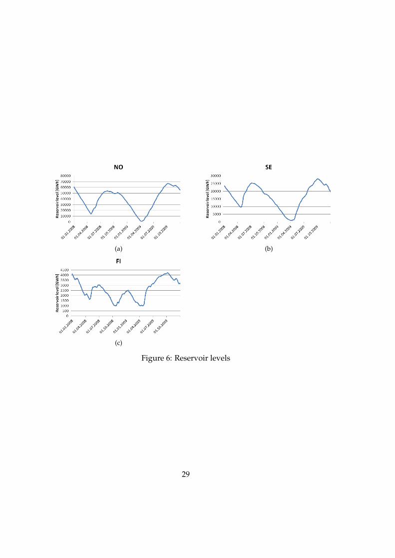
The dual values of the water balance constraint (4.5) can be seen as the marginalvalue of having one more unit of water available. According to the theory pre-sented in 3.2.1, this is known as the water value and is the marginal cost of usingwater. The water values can be seen in Figure 5. Because the objective functiondecreases as the constraint is relaxed, the sign is negative. The reservoir levelsare shown in Figure 6. Although the reservoirs never reach the maximum levelin any of the areas during the scheduling period, they all reach the minimumreservoir level around the same time. This time is around the beginning of April2009, and if we compare these results with the inflow data in Figure 3 we cansee that it is at this time in 2009 that the melting season starts.

26

(a) (b)

(c) (d)

Figure 4: Power prices

27

(a) (b)

(c)

Figure 5: Water values

28

(a) (b)

(c)

Figure 6: Reservoir levels

29

5.1.3 Analysis

The optimal generation is found by the optimizer using a merit order list. Thisincludes ranking the available generation units according to their marginal cost,and engaging them in that order until demand is covered or their capacities aremet. The power price in the outside regions can be seen as a marginal cost, andis ranked by the optimizer in the same way as a generator with the transmissioncapacity as the limit. The price of the most expensive generation unit or outsideregion price sets the dual value of the power balance constraint which can beseen as the power price. The water values are used as the marginal cost ofhydropower.

By comparing the power prices in Figure 4 and the water values in Figure 5 inthe three hydro-producing countries, we can see a strong connection. Especiallyin Norway, the power prices and the water values are exactly the same (butwith opposite sign). This means that it is always the water value that governsthe power price in Norway. By comparing this to the generation capacities inTable 1, we see that most of the generation capacity is from hydropower inNorway. In Sweden and Finland there are more fluctuations, but we can still seea strong connection. The water values are major price-drivers, but at times thereare other units in these areas determining the power price. For Denmark, theprice fluctuates during the whole scheduling period. They do not have hydro-power, but they have strong transmission capacity from Norway, Sweden andGermany. So the price in Denmark is more vulnerable to changes to the Germanpower prices than the water values in Norway and Sweden.

The minimum reservoir levels of 1000 GWh are reached in the beginning ofApril in 2009. So in the model, it is optimal to empty the reservoirs as muchas possible right before the melting season starts in 2009. At the same time thewater values in Norway and Sweden drop, and hence the power prices drop.This can be explained in relation to the model being deterministic. Becauseinflow values are perfectly predictable, the optimizer chooses to decrease thevalue of the water right at the beginning of the melting season when the wateris at the minimum level. In reality, because of the stochastic nature of inflows,the water value is inversely proportional to the reservoir level. This points to amajor flaw in using deterministic values.

It can also be noted that there is never any gap between the production andthe consumption. There is always enough power to satisfy demand, and thegap cost of 1000 €/MWh is never used. The highest power prices are seen inDenmark during December 2008, and the powe price reaches more than 300€/MWh. However because we have left out wind power completely, these

30

prices would not be reached in reality.

5.2 Analysis of a single time period

To better understand the model, we study a single time period to see what isgoing on. The period chosen is period 10 000, and this corresponds to the hour4pm-5pm on the 20th of February 2009.

The generation costs are seen in Table 6, while the actual generation is seen inTable 7. From Table 8, we see that in all the three hydro-producing countries,it is the water value that sets the power price in this particular time period.The power prices in outside areas are seen in Table 9, and from this we cansee that it is the German power price that sets the Danish power price in thishour. This price is slightly higher than in the rest of the Nordic region. Ineach area, only the units which are below the power price are set into use, andby comparing to their respective capacities from Table 1 we can see that theNuclear and CoalCondensing units are producing on max capacity. Ofcoursethe 0 €/MWh for hydro generation is misleading, as the water value is actuallythe marginal cost.

Table 6: Generation costs

Generator type Cost [€/MWh]Hydro 0.0Nuclear 15.0CoalCondensing 28.2CoalExtraction 28.8GasExtraction 47.4CCGT 34.0GasTurbine 48.0

31

Table 7: Generation by type (average hourly production)

Generator type Area Generation [MW]Hydro NO 20139Hydro SE 8735Hydro FI 2324Nuclear SE 8938Nuclear FI 2646CoalCondensing SE 2271CoalCondensing FI 2935CoalCondensing DK 784

Table 8: Shadow prices

NO SE FI DKDual costs 41.4 41.9 42.3 43.6

Water values -41.4 -41.9 -42.3

Table 9: Outside power prices [€/MWh]

GE NL PO43.6 42.7 39.3

32

From Table 10, we see which transmission lines are in use and the amount trans-ferred in these lines. We see that the power flow in the transmission lines are attheir maximum values when we compare to the capacities in Table 4 in all thetransmission lines except for in the line from Denmark to Germany. This line isshown in italic text and is not transmitting at the limit.

Table 10: Border flow

From area To area Border flow [MW]NO DK 950NO FI 100SE DK 1980NO NL 700SE GE 600DK GE 160PO SE 600

It is typical in linear programming that variables are at their limits, so it is notsurprising to see that this is the case for the border flow and generation vari-ables.

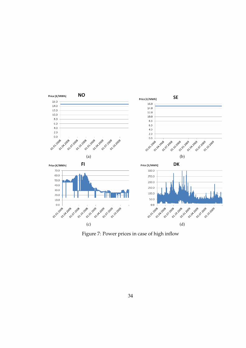
5.3 Other inflow scenarios

To investigate the effect that the inflow has on the output, two other inflowscenarios are run in the model; one where the inflow is 25% higher than in theoriginal case for all time periods, and one where the inflow is 25% lower. Theresults on the power prices are shown in Figure 7 (high inflow) and in Figure 8(low inflow).

33

(a) (b)

(c) (d)

Figure 7: Power prices in case of high inflow

34

(a) (b)

(c) (d)

Figure 8: Power prices in case of low inflow

35

From these figures we see that the power prices are very much affected by theinflow levels. The objective function value has not been discussed earlier be-cause it has little relevance in this model. The factors that we are interested inare the dual values of the constraints and the values of the variables. Howeverit was noted that the objective value (that is, the total cost of the system oper-ation) increased by more than 100 % in the low inflow scenario. In the highinflow case, the objective function value decreased by more than 100%.

36

6 Conclusion and further work

6.1 Conclusion

This paper has analyzed the optimal operation of a hydrothermal power sys-tem. The particular area of study has been the Nordic power system, and this ischaracterized by a large amount of hydropower. The handling of reservoirs istherefore of great interest, and different approaches to reservoir-handling havebeen studied and evaluated. A linear deterministic single-reservoir model wasformulated and implemented in XpressMP. The model successfully allocatedthe different generating units and transmission according to the demand in eachperiod, minimizing the total system cost during the planning horizon. Powerprices for the Nordic countries together with reservoir levels were forecasted onan hourly resolution for a two-year period. Three inflow scenarios were testedin the model, and the results from running the deterministic model on the dif-ferent inflow scenarios showed the major influence that inflow scenario has onthe power price. According to the results, reservoirs are completely emptied tothe minimum level just before the second inflow season starts.

The above conclusions address the issue that deterministic representation ofstochastic factors will not give a reliable result. Only if the expected scenarioturns out to materialize, can the model guarantee optimality. The chance forthis is minimal, and a stochastic modeling approach should be preferred.

6.2 Further work

In this section, improvements to the model are suggested.

6.2.1 Improving the deterministic model

A list of issues that should be considered for further development of the modelis given here:

• In the model, it is assumed that all generators are available at all timesduring the planning period. In reality however, this is not the case asgenerators need to be disconnected from the system due to maintenance.This can be both planned maintenance or a fault forcing them to shutdown.

37

• Shutting down and starting up generators does not come without a costas implicitly implied in the model, and the start-up costs for the differentgenerators should be included in the model.

• Windpower generation is left out completely of the model, and as seen inthe results, this has major implications on the forecasted power price inDenmark.

• Transmission losses should be proportional to the power transferred, nota constant percentage as is used in the model.

• Exchange with Estonia and Russia is left out of the model.

The improvements listed above are all possible to implement into the modelwithout much difficulties. Another weakness of the model that is not simple toimprove, is the use of aggregated reservoirs for each country. Localized spillagecan occur that is not captured by the model. Also, with the minimum reservoirlevel of 1000 GWh, many smaller reservoirs would run dry. The way to improvethis in the model would be to use smaller price areas based on river systemsinstead of countries. There is much data that must be collected if the areas usedwere to change, but the same MOSEL-code can in principle be used.

6.2.2 Stochastic programming

The results from running the model with different inflow scenarios implied thatdeterministic inflows represent a serious flaw in the model. If the proposedgeneration plan was used in reality, there would be a high risk of shortageand spillage because the risks for these are not represented in the model. Amodel that handles uncertainty should be preferred, with the most importantuncertainty being the inflow. Relevant models are presented in Section 3, and alarge task with implementing a stochastic model is to get different inflow sce-narios.

38

References

R. Bellman. Dynamic programing. Princeton, New Jersey, 1957.

J.F. Benders. Partitioning procedures for solving mixed-variables programmingproblems. Numerische Mathematik, 4(1):238–252, 1962.

J.R. Birge. Decomposition and partitioning methods for multistage stochasticlinear programs. Operations Research, 33:989–1007, 1985.

N. Buras. Conjunctive operation of dams and aquifers. American Society of CivilEngineering, 89(6):111–131, 1963.

G. Doorman. Hydro Power Scheduling. NTNU, 2009.

O. Egeland, J. Hegge, E. Kylling, and J. Nes. The extended power poolmodel—operation planning of multi-river and multi-reservoir hydrodomi-nated power production system—a hierarchial approach. In 1982 CIGREMeeting, Paris, 1982.

R.W. Ferrero, J.F. Rivera, and S.M. Shahidehpour. A dynamic programmingtwo-stage algorithm for long-term hydrothermal scheduling of multireser-voir systems. Power Systems, IEEE Transactions on, 13(4):1534–1540, 1998.

A. Gjelsvik. Stochastic seasonal planning in multireservoir hydroelectric powersystems by differential dynamic programming. Modeling, Identification andControl, 3(3):131–149, 1982.

A. Gjelsvik, TA Røtting, and J. Røynstrand. Long-term scheduling of hydro-thermal power systems. In Hydropower, volume 92, pages 539–546, 1992.

A. Halseth. Market power in the nordic electricity market. Utilities Policy, 7(4):259–268, 1999.

J. Lindqvist. Operation of a hydrothermal electric system: A multistage decisionprocess. Power Apparatus and Systems, Part III. Transactions of the AmericanInstitute of Electrical Engineers, 81(3):1–6, 1962.

J. Lundgren, M. Rönnqvist, and P. Varbrand. Optimazation. Studentlitteratur,2010.

P. Massé. Les réserves et la régulation de l’avenir dans la vie économique. Hermann& Cie., 1946.

K.D.W. Nandalal and J. Bogárdi. Dynamic programming based operation of reser-voirs: applicability and limits. Cambridge Univ Pr, 2007.

39

M.V.F. Pereira and L. Pinto. Stochastic optimization of a multireservoir hydro-electric system: A decomposition approach. Water Resources Research, 21(6):779–792, 1985.

M.V.F. Pereira and L. Pinto. Multi-stage stochastic optimization applied to en-ergy planning. Mathematical Programming, 52(1):359–375, 1991.

W.B. Powell. Approximate Dynamic Programming: Solving the curses of dimension-ality, volume 703. Wiley-Blackwell, 2007.

T.J. Scott and E.G. Read. Modelling hydro reservoir operation in a deregulatedelectricity market. International Transactions in Operational Research, 3(3-4):243–253, 1996.

S. Soares and A.A.F.M. Carneiro. Optimal operation of reservoirs for electricgeneration. Power Delivery, IEEE Transactions on, 6(3):1101–1107, 1991.

S. Stage and Y. Larsson. Incremental cost of water power. Power Apparatus andSystems, Part III. Transactions of the American Institute of Electrical Engineers, 80(3):361–364, 1961.

A. Turgeon. Optimal operation of multireservoir power systems with stochasticinflows. Water Resources Research, 16(2):275–283, 1980.

I. Wangensteen. Power system economics: the Nordic electricity market. Tapir aca-demic press, 2007.

O. Wolfgang, A. Haugstad, B. Mo, A. Gjelsvik, I. Wangensteen, and G. Door-man. Hydro reservoir handling in norway before and after deregulation. En-ergy, 34(10):1642–1651, 2009.

S. Yakowitz. Dynamic programming applications in water resources. WaterResources Research, 18(4):673–696, 1982.

W.W.G. Yeh. Reservoir management and operations models: A state-of-the-artreview. Water resources research, 21(12):1797–1818, 1985.

Z. Yu, F.T. Sparrow, and B.H. Bowen. A new long-term hydro productionscheduling method for maximizing the profit of hydroelectric systems. PowerSystems, IEEE Transactions on, 13(1):66–71, 1998.

40

Appendix A - Mosel code

41