An Orientation-space Super Sampling Technique for Six

Fundamenta Informaticae 146 (2016) 219–230 219

DOI 10.3233/FI-2016-1383

IOS Press

An Orientation-space Super Sampling Technique forSix-dimensional Diffraction Contrast Tomography

Nicola Vigano∗

MATEIS, INSA Lyon, CNRS (UMR5510), Univ. Lyon, F-69621 Lyon, France, and

ESRF, The European Synchrotron, F-38043 Grenoble, France

[email protected]

Kees Joost Batenburg∗

CWI, Amsterdam, 1098 XG Amsterdam, The Netherlands, and

University of Leiden, Mathematical Institute, 2300 RA Leiden, The Netherlands

Wolfgang LudwigMATEIS, INSA Lyon, CNRS (UMR5510), Univ. Lyon, F-69621 Lyon, France, and

ESRF, The European Synchrotron, F-38043 Grenoble, France

Abstract. Diffraction contrast tomography (DCT) is an X-ray full-field imaging technique thatallows for the non-destructive three-dimensional investigation of polycrystalline materials andthe determination of the physical and morphological properties of their crystallographic do-mains, called grains. This task is considered more and more challenging with the increasingintra-granular deformation, also known as orientation-spread. The recent introduction of a six-dimensional reconstruction framework in DCT (6D-DCT) has proven to be able to address theintra-granular crystal orientation for moderately deformed materials.The approach used in 6D-DCT, which is an extended sampling of the six-dimensional com-bined position-orientation space, has a linear scaling between the number of sampled orienta-tions, which determine the orientation-space resolution of the problem, and computer memoryusage. As a result, the reconstruction of more deformed materials is limited by their high re-source requirements from a memory and computational point of view, which can easily becometoo demanding for the currently available computer technologies.In this article we propose a super-sampling method for the orientation-space representation ofthe six-dimensional DCT framework that enables the reconstruction of more deformed cases byreducing the impact on system memory, at the expense of longer reconstruction times. The use ofsuper-sampling can further improve the quality and accuracy of the reconstructions, especially incases where memory restrictions force us to adapt to inadequate (undersampled) orientation-spacesampling.

∗Also works: University of Antwerp, iMinds-Vision Lab, B-2610 Antwerp, Belgium.Address for correspondence: MATEIS, INSA Lyon, CNRS (UMR5510), Universite de Lyon, F-69621 Lyon, France.

Received July 2016; revised July 2016.

220 N. Vigano et al. / An Orientation-space Super Sampling Technique for Six-dimensional Diffraction...

1. Introduction

X-rays, through the use of computed tomography (CT), allow for non-destructive three-dimensionalinvestigation of materials’ inner structure and properties. X-ray diffraction in particular probes thecrystallographic properties of the analysed objects.

Diffraction contrast tomography (DCT), is an extended-beam near-field technique in the domainof three-dimensional X-ray microscopy. Thanks to the illumination of extended three-dimensionalregions in the analysed objects, DCT allows for fast measurements, and so, it also allows to follow thetime evolution of crystalline materials, with high spatial resolution.

The original focus of DCT was of the reconstruction of the grain shape and orientation in unde-formed or nearly-undeformed materials. With the advent of [1], which proposes a six-dimensionalformulation of the DCT reconstruction problem (6D-DCT), and the following work based on the saidsix-dimensional model [2, 3], the focus has been shifted more and more towards the sub-grain orien-tation determination in moderately deformed materials. Especially in [2], where 6D-DCT was provento be able to retrieve the local orientation of large textured regions, also the limits of this approachwere exposed.

The six-dimensional model is based on a discrete sampling of both the real-space, and the ori-entation-space occupied by a given grain, which suffers from the so called “curse of dimensionality”,where the increased number of dimensions in a sampling problem, increases the associated memoryrequirements in an exponential way. The reconstruction of large real-space regions, exhibiting moder-ate to high orientation-spreads, implicates that large amounts of memory are needed for the computeralgorithms to reconstruct these regions.

While the real-space resolution in a DCT reconstruction is linked to the acquisition resolution, theorientation-space resolution is determined by the size of the orientation-space bounding box, where weexpect to find all the possible orientations present in the to-be-reconstructed region, and the number ofsampled points. Moderate to high deformations imply larger orientation-space bounding boxes, whereto sample orientations. As a consequence, for constant resolution, one would need considerably moreorientations, than for lower levels of deformation, but memory is limited and at some point we haveto make a compromise and increase the sampling interval (i.e. decrease the ultimate resolution).

In this article we present a super-sampling framework in the orientation-space to alleviate theshortcomings linked to these memory constrained problems, and possibly to allow for the reconstruc-tion of extreme cases which were previously considered impossible to solve with nowadays computertechnology.

2. Method

We are now going to introduce the diffraction geometry used in DCT, then we will describe howthis translates to its projection model and finally we will discuss the super-sampling extension of thismodel.

2.1. Diffraction geometry

The usual setup of diffraction contrast tomography, when using a monochromatic beam, consists ofa rotation stage where the sample is positioned, and an high resolution imaging detector positionedimmediately behind the sample.

N. Vigano et al. / An Orientation-space Super Sampling Technique for Six-dimensional Diffraction... 221

Figure 1: Diffraction geometry of a DCT experiment.

As the sample rotates by angle ω, it gives rise to diffracted beams each time the Bragg conditionis met for one of the grains. Some of those diffracted beams will intersect the detector, and giverise to diffraction spots, which, in the absence of intra-granular orientation spread, correspond to2D projections of the 3D grain volume. After diffraction spot segmentation and indexation basedon Friedel pairs (hkl and hkl reflections of the same grain observed for ω0 and ω0 + 180◦) the 3Dgrain structure can be reconstructed by means of iterative tomographic reconstruction techniques. Thereader interested in details concerning the setup, acquisition procedures and initial processing stepslike segmentation, Friedel pair matching and indexation of near-field X-ray diffraction data is referredto [4] and [5].

In the presence of non-negligible intra-granular orientation spread, the parallel projection assump-tion used in conventional (three-dimensional) DCT gets violated. Each of the sub-orientations presentin a grain is associated to a slightly different projection geometry and the diffraction signal associatedto a given Bragg reflection is observed as a distorted, three-dimensional diffraction volume, whichthen takes the name of diffraction “blob”. It is parametrized by two spatial coordinates u and v (de-tector pixel coordinates) and a rotation angle ω (image number). An alternative parametrization of theblob coordinates, instead of the triplet (ω, u, v), is given by the triplet (ω, θ, η), where the angle θ isthe aperture angle typical of an hkl-family, and η is the angle between the (u, v) position of the blobon the detector and the projection of the rotation axis on the detector, having the projected center ofthe diffracting grain as vertex (fig. 1).

2.2. Projection model in Diffraction Contrast Tomography

As previously introduced in [1], the single grain reconstruction problem can be cast as the solution ofan underdetermined linear system:

Ax = b (1)

where x is the volume to be reconstructed, b represents the images recorded on the detector, and A isthe so called projection matrix, which embodies the projection geometry of the tomographic problem.

If the reconstruction takes the local orientations in the voxels into account, it will be set in a six-dimensional space, given by the outer product of the real-space and the orientation-space defined as:


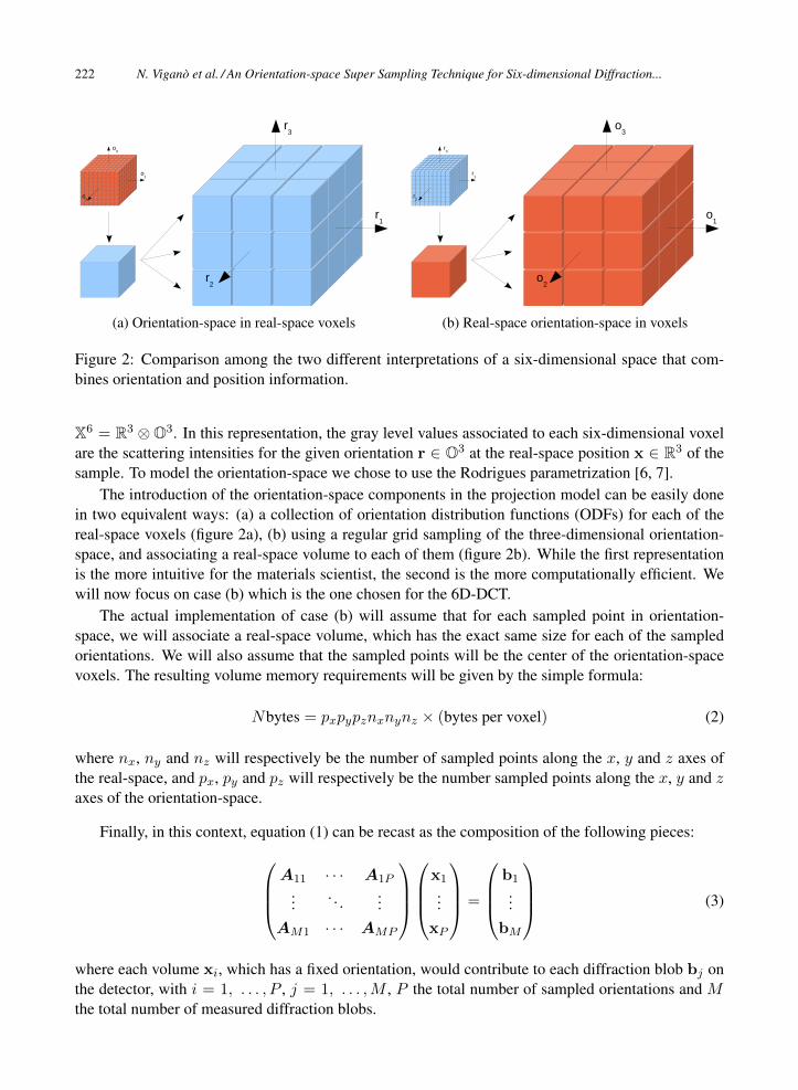
(a) Orientation-space in real-space voxels (b) Real-space orientation-space in voxels

Figure 2: Comparison among the two different interpretations of a six-dimensional space that com-bines orientation and position information.

X6 = R3 ⊗O3. In this representation, the gray level values associated to each six-dimensional voxelare the scattering intensities for the given orientation r ∈ O3 at the real-space position x ∈ R3 of thesample. To model the orientation-space we chose to use the Rodrigues parametrization [6, 7].

The introduction of the orientation-space components in the projection model can be easily donein two equivalent ways: (a) a collection of orientation distribution functions (ODFs) for each of thereal-space voxels (figure 2a), (b) using a regular grid sampling of the three-dimensional orientation-space, and associating a real-space volume to each of them (figure 2b). While the first representationis the more intuitive for the materials scientist, the second is the more computationally efficient. Wewill now focus on case (b) which is the one chosen for the 6D-DCT.

The actual implementation of case (b) will assume that for each sampled point in orientation-space, we will associate a real-space volume, which has the exact same size for each of the sampledorientations. We will also assume that the sampled points will be the center of the orientation-spacevoxels. The resulting volume memory requirements will be given by the simple formula:

Nbytes = pxpypznxnynz × (bytes per voxel) (2)

where nx, ny and nz will respectively be the number of sampled points along the x, y and z axes ofthe real-space, and px, py and pz will respectively be the number sampled points along the x, y and zaxes of the orientation-space.

Finally, in this context, equation (1) can be recast as the composition of the following pieces:A11 · · · A1P

.... . .

...AM1 · · · AMP

x1

...xP

=

b1

...bM

(3)

where each volume xi, which has a fixed orientation, would contribute to each diffraction blob bj onthe detector, with i = 1, . . . , P , j = 1, . . . ,M , P the total number of sampled orientations and Mthe total number of measured diffraction blobs.


2.3. Super-sampled projection model

As the projection matrix model is based on a discrete sampling of the six-dimensional space formedby the outer product of a three-dimensional real-space and a three-dimensional orientation space, theresolution in the sampling grid will play an important role for determining the accuracy of the tomo-graphic model itself. As mentioned earlier, the real-space sampling resolution is given by the detectorpixel size, which translates into the real-space voxel size. The orientation-space resolution insteadis not fixed by the experiment alone, but also depends on material characteristics. This means thatin memory constrained cases, where large orientation-space bounding boxes are used, in conjunctionwith having to deal with large regions in real-space, also a considerable number of orientations willbe needed.

From equation (2), it follows that for an increase of resolution of a factor 2 in orientation-space,the memory requirements would become 23 = 8 times larger. For a constant number N of elementsin x, this implies that for growing orientation-space bounding boxes, associated with large real-spacebounding boxes, a lower orientation-space resolution could be expected. As a consequence, this wouldlead to the distance among the sampled points to grow, and to the assumption of one single chosenorientation to approximate the whole associated orientation-space voxel to fail.

In real-space, a strip model of the projection rays could help with moderate inhomogeneity of thevoxel size compared to the detector pixel sizes, especially when the pixels are larger than the voxels,because the strips would intercept all the voxels having an overlap with the strip. In this case, instead,Joseph’s method wouldn’t be able to associate some voxels to the related detector pixels, but variousoversampling techniques exist to solve this problem, like the super-sampling method used in [8] fortheir super-resolution application.

Since in orientation-space each point determines a projection geometry in real-space, it is notobvious how to model a projection geometry corresponding to the integral of a three-dimensionalinterval of orientations.

It is in fact easier to start from the back-projection super-sampling technique presented in [8], thatis based on a sampling approach, and model a similar type of orientation super-sampling.

The orientation space voxels, as shown in the inset of figure (3), instead of being represented by asingle sampled point in the center of the orientation space volume forming the said voxel, they couldbe divided into S = s3 sub-voxels, that would forward and back project the same associated real-space volume, but with slightly different orientations given by the centers of the new sub-voxels andprojection coefficients of 1/S instead of 1. The new projection matrix would then look like:

Ax =P∑i

S∑j

1

SAijxi = b (4)

where for a given volume i, the sub-matrices Ai = {Ai1,Ai2, . . . ,AiS} are the associated orientation-space sub-voxel sampled orientations.

For memory constrained configurations, the use of this type of super-sampling can alleviate con-siderably artifacts due to otherwise poor sampling. In fact, it increases by a factor s the coverage of theorientation-space, resulting in S = s3 times finer sampling. On the other hand, this doesn’t translatein an effective increase in orientation-space resolution by a factor s, for which we would then need touse SP volumes, instead of the P volumes used in this configuration.


Figure 3: Orientation space super sampling, as shown by the top right front voxel of the sampled grid.While the usual sampling would pick the center of the voxels associated to the volumes like in figure2b, in this case we instead pick the centers of the sub-voxels and associate all of them with the samereal-space volume.

2.4. Reconstruction algorithm

The reconstruction algorithm is the same that was used in [2], and it is based on a recast of equation(1) into a minimization problem, where the solution of the algorithm is the vector that minimizes thefollowing functional:

x∗ = argminx||Ax− b||2 + λ|| (|∇Sx|) ||1 (5a)

subject to: x ≥ 0 (5b)

where S is the operator that sums all the components in orientation-space for each real-space voxel,and the l1-norm over the absolute value of the gradient is the total variation operator TV (·) [9, 10].More precisely, the operator S is defined as the projection S : X6 = R3 ⊗ O3 → R3 from the six-dimensional space X6 to the three-dimensional real-space R3. In fact, if we sum all the contributionsfrom the orientation-space to each position in real-space, we obtain a pure positional three-dimensionalvolume that contains the information about the shape of the reconstructed grain.

As a result, thanks to the addition of the TV (·) operator, the algorithm resolving the minimizationproblem expressed in equation (5), minimizes the projection distance from the detector images, andpromotes the grain boundary sharpness and the grey level homogeneity inside the grain at the sametime.

For the solution of the functional in equation (5) we used the same algorithmic instance proposedin [1].

2.5. Hardware and software implementation details

The reconstructions were performed on a desktop machine with two Intelr Xeonr CPUs E5-2630working at 2.30GHz, an NVIDIAr GeForce GTX 980 GPU card and 64GB of RAM. The soft-


ware was implemented in Matlab1 and C++, using the ASTRA Toolbox2 for the projection and back-projection of the volumes.

3. Results and discussion

To verify the model established in the previous section, we decided to use highly deformed three-dimensional synthetic dataset, which is based on the one used in [1]. The new dataset instance is stillbased on a 50 × 50 × 50 voxels volume, where the deformation pattern has been rescaled, from anorientation spread of 1 degree to 5 degrees across the volume.

While using the same phantom, we decided to perform two different tests at two different orientation-space sampling resolutions, to test the behaviour of the super-sampling framework in two differentscenarios: (a) poor orientation-space resolution, to see if this extension was able to mitigate the prob-lem due to a bad coverage of orientation-space, (b) decent but not optimal orientation-space resolution,to see if the proposed framework would still be able to push the reconstruction towards better results.

The 3.32× 3.10× 3.27 degrees orientation-space bounding box is sampled using 8× 7× 8 and18× 16× 17 sampling points respectively.

We then compared the shapes of the reconstructed objects and the orientation-space accuracy ofthe reconstruction with and without various parameters s of super-sampling. In all the reconstructions60 blobs were used.

3.1. Orientation-space resolution

Before entering the discussion about the results we would like to briefly discuss the maximum expectedresolution for this type of diffraction experiments in orientation-space, and how to compute the actualresolution in the reconstructed region of interest.

As it happens for the position-space, where the maximum resolution in the one determined bythe detector pixel size, for the orientation-space, the maximum achievable resolution will also bedetermined by the experimental conditions, but with a slightly higher degree of complexity.

The parallelism between the two spaces is even more obvious if we think that for a fixed position inorientation-space, a point (ω, u, v) on the detector defines a projection line in real-space, and for a fixedpoint in real-space, a position (ω, θ, η) on the detector defines a line in orientation-space [11, 12]. Thismeans that the maximum resolution on the detector for (ω, θ, η) will define the maximum resolutionin orientation-space.

Since the z-axis is aligned with the sample rotation axis, the experimental integration stepping ofthe ω angle will directly translate into the resolution along the z-axis of the orientation-space. Thismeans that:

rz,max = δω (6)

where rz,max stands for maximum resolution along the z-axis and δω is the experimental ω integrationstep.

For what concerns the x-axis and the y-axis the resolution will be related to the minimum detectableangle in η, which in turn depends on several factors, including the distance of the detector from the1Registered trademark of MathWorks2https://github.com/astra-toolbox


sample, the hkl-family of each blob, and the effective size of the detector pixels. If we define theeffective detector pixel size as:

∆pixel = | cos(η0)|∆u+ | sin(η0)|∆v (7)

where ∆u and ∆v are the pixel edge sizes in the u and v directions respectively, and η0 is the averageη of the considered blob, we can compute the maximum achievable resolution along the x-axis and they-axis as the following:

rx,y,max = δη = tan−1

(∆pixeldblob

)= tan−1

(∆pixel

Ddetector tan (2θ)

)(8)

where dblob is the distance between the centroid of the blob and the projection of the grain center onthe detector, and Ddetector is the distance between the grain and the detector (fig. 1).

So, by taking a δω = 0.1 degrees, ddetector = 6 mm, a maximum θ = 5.73 degrees, an associatedη = 42 degrees and ∆u = ∆v = 1 µm, we have that the maximum achievable resolutions inorientation-space will be:

rz,max = 0.1 degrees (9a)

rx,y,max = tan−1

(1µm

6× 103µm× tan (2× 5.73 degrees)

)= 0.067 degrees (9b)

Finally, if we compute the orientation-space sampling resolution r in one direction d as:

rd =ld

(pd − 1)(10)

where ld is the size of the bounding box and pd is number of sampling points in that specific direction,we obtain resolutions of 0.47 × 0.51 × 0.46 degrees and 0.19 × 0.20 × 0.20 degrees, respectivelyfor the two test cases, which are well above the smallest achievable precisions, from the experimentalconditions.

On the other hand, to reach the maximum allowed resolution in orientation-space, we would needa grid of 34 × 47 × 49 sampling points for the example in this article. With a real-space volumecomposed by 72 × 72 × 72 single precision floating point voxels, according to equation (2), wewould need almost 110GB of RAM to store the six-dimensional representation of the reconstructionspace. Since the algorithm needs two copies for each of those volumes, the total requirements willbe 220GB of RAM, making this relatively small test case quite challenging for the currently availableworkstations.

3.2. Low resolution reconstructions

We here analyse the results from the (a) scenario, which had a memory occupation of only 638 MBsfor the volumes used, leading to a ∼ 2 GBs total memory occupation.

The regular reconstruction took 530s ' 9min, in comparison with the super-sampled reconstruc-tion that took 2707s ' 45m with a super-sampling factor s = 2, and 7793s ' 2h10min with asuper-sampling factor s = 3.


(a) Phantom (b) Normal reconstruction (c) Super-sampling s = 2 (d) Super-sampling s = 3

Figure 4: Comparison of the shape retrieved by the reconstructions for a 8 × 7 × 8 sampling pointsgrid, in the normal and super-sampled case with super-sampling factors s = 2 and s = 3.

5040

3020

1000

10

20

30

40

10

0

50

40

30

20

50

(a) Phantom

5040

3020

1000

10

20

30

40

10

0

50

40

30

20

50

(b) Normal reconstruction

5040

3020

1000

10

20

30

40

10

0

50

40

30

20

50

(c) Super-sampling s = 2

5040

3020

1000

10

20

30

40

10

0

50

40

30

20

50

(d) Super-sampling s = 3

Figure 5: Comparison of the orientation-space morphology reconstructed with a sampling of 8×7×8grid points, in the normal and super-sampled case with super-sampling factors s = 2 and s = 3.

As it can be seen in figure (4b), the chosen resolution is not sufficient to reconstruct the shape of thecubic grain used in this synthetic test case. From figure (4c) instead we see that a small oversamplingfactor of s = 2 already improves the reconstruction of the selected slice, even if the orientation-spacecoverage is still not enough to achieve a decent result. Figure (4d) suggests that a bigger super-sampling factor of s = 3 might help to further alleviate the shortcomings of a bad orientation-spacesampling resolution, for what concerns the shape and homogeneity of the reconstructed object.

In figure (5), a different aspect is taken into account: we look at the orientation-space reconstruc-tion accuracy for the different reconstruction parameters. In this figure, we use the orientation coloringused in [1], to visualize orientation domains in an easily recognizable way for the human eye, whereeach color is associated with a region in the sample orientation-space, and where contiguous regionshave similar colors.

Again, as noted for the shape of the reconstructed object, an oversampling factor s = 2 (figure 5c),and s = 3 (figure 5d), give a visible improvement over the reconstructions without any oversampling,which is in line with the expectations from figure (4b).

3.3. Moderate resolution reconstructions

In the higher resolution case (b), which needed 6.8 GBs for the volumes, leading to a ∼ 15 GBstotal memory occupation, the regular reconstruction took 5679s ' 1h34min, in comparison with thesuper-sampled reconstruction that took 26947s ' 7h29min, with super-sampling parameter s = 2.


(a) Phantom (b) Normal reconstruction (c) Super-sampling reconstruction

Figure 6: Comparison of the shape retrieved by the reconstructions for a 18×16×17 sampling pointsgrid, in the normal and super-sampled case with a super-sampling factor s = 2.

5040

3020

1000

10

20

30

40

10

0

50

40

30

20

50

(a) Phantom

5040

3020

1000

10

20

30

40

10

0

50

40

30

20

50

(b) Normal reconstruction

5040

3020

1000

10

20

30

40

10

0

50

40

30

20

50

(c) Super-sampling reconstruction

Figure 7: Comparison of the orientation-space morphology reconstructed with a sampling of 18 ×16× 17 grid points, in the normal and super-sampled case with a super-sampling factor s = 2.

In this scenario, the higher super-sampling values like s = 3 from the previous case were nottested, due to higher needs in term of computational power and the moderate advantage in terms ofreconstruction quality.

As expected, figure (6) as compared to figure (4), shows that by increasing the orientation-spaceresolution, even without any super-sampling, the algorithm already gives a better reconstruction forthis test case. However, the quality of the reconstruction can be further enhanced by introducing theoversampling with a factor of s = 2. In fact, figure (6c) shows a clearly smoother and space fillingreconstruction than figure (6b).

We observe the same behavior in figure (7), where especially the interfaces among the differentorientation domains were resolved with higher precision in the super-sampled reconstruction.

4. Conclusions and outlook

As shown in the previous section, in both study cases, the proposed super-sampling method providedbetter results both in terms of grain shape reconstruction quality and local orientation determinationaccuracy.


The biggest improvement obtained thanks to this super-sampling technique was obviously in thelow resolution case study, where the non super-sampled reconstruction (figures 4b and 5b) showedextremely poor reconstruction quality. In fact, the super-sampled reconstruction gave visible improve-ments both in the reconstruction of the shape, and in the determination of the local orientation (figures4c and 5c), without however being able to outperform the higher resolution reconstruction of the sec-ond test case.

In spite of the fact that higher orientation-space super-sampling parameters s can significantlyimprove the orientation-space representation of the chosen sampling, it cannot actually increase theorientation-space resolution. This means that it has no influence on the formula in equation (10),and that it is not possible to achieve a better result using the coarse sampling of 8 × 7 × 8 withsuper-sampling parameter s = 2 or s = 3, instead of the non-supersampled 18 × 16 × 17 grid. Bycomparing figure (4d) with figure (6b) and figure (5d) with figure (7b), the results indeed confirmthat the orientation-space super-sampling cannot fix a bad orientation-space sampling. Moreover,the computational cost of higher super-sampling parameters s, can become prohibitive for biggerreconstruction problems.

In conclusion we see this super-sampling technique as a good tool for allowing to retrieve usefulinformation from memory limited cases, where the size of the real-space volumes, and the availablememory, do limit the quality of coverage of the orientation-space. The longer computation times arepaid off by the increased accuracy of the projector, and as a consequence, of the increased quality ofthe reconstructions.

In the future, in addition to this orientation-space super-sampling technique, also other strategiescould be incorporated to enable the analysis of more difficult and interesting scientific scenarios. Forinstance, if we allow for a small decrease in real-space resolution, we could imagine the combineduse of this orientation-space super-sampling with a real-space super-sampling acting on binned real-space volumes. The real-space super-sampling would balance the real-space voxels’ increased size,while at the same time allowing for an increased orientation-space resolution, at constant memoryconsumption.

As a final remark, since the biggest cost center in the reconstruction resides in the forward-projection and back-projection of the real-space volumes, it is reasonable to assume that in the future,when newer and more powerful graphics chipsets will be available, the computation times could begreatly reduced. In addition, the projection of each volume is independent of the projection of everyother volume, except for a small part of the calculation. This means that it is also possible to runmultiple volume projections at the same time if multiple GPUs are available. As a result, with modernmulti-GPUs solutions and the use of the ASTRA library, the reconstruction speed could already be atleast doubled, with minimal changes in the code.

Acknowledgments

NV and WL acknowledge financial support of the French National Research Agency (ANR), project:ANR 2010 BLAN 0935, and the German Research Foundation (DFG), priority programme: SPP 1466.

KJB acknowledges financial support of the Netherlands Organization for Scientific Research(NWO), project nr. 639.072.005.

The authors acknowledge COST Action MP1207 for networking support.NV would like to thank Willem Jan Palenstijn for the precious discussions.


References[1] Vigano N, Ludwig W, Batenburg KJ. Reconstruction of local orientation in grains using a discrete rep-

resentation of orientation space. Journal of Applied Crystallography. 2014 oct;47(6):1826–1840. doi:10.1107/S1600576714020147.

[2] Vigano N, Tanguy A, Hallais S, Dimanov A, Bornert M, Batenburg KJ, et al. Three-dimensional full-fieldX-ray orientation microscopy. Scientific Reports. 2016 feb;6. Available from: http://www.nature.

com/articles/srep20618. doi:10.1038/srep20618.

[3] Vigano N, Nervo L, Valzania L, Singh G, Preuss M, Batenburg KJ, et al. A feasibility study of full-fieldX-ray orientation microscopy at the onset of deformation twinning. Journal of Applied Crystallography.2016 apr;49(2). doi:10.1107/S1600576716002302.

[4] Ludwig W, Reischig P, King A, Herbig M, Lauridsen EM, Johnson G, et al. Three-dimensional grainmapping by x-ray diffraction contrast tomography and the use of Friedel pairs in diffraction data analysis.The Review of scientific instruments. 2009 mar;80(3):033905. doi:10.1063/1.3100200.

[5] Reischig P, King A, Nervo L, Vigano N, Guilhem Y, Palenstijn WJ, et al. Advances in X-ray diffractioncontrast tomography: flexibility in the setup geometry and application to multiphase materials. Journal ofApplied Crystallography. 2013 mar;46(2):297–311. doi:10.1107/S0021889813002604.

[6] Frank FC. Orientation mapping. Metallurgical Transactions A. 1988;19(3):403–408.doi:10.1007/BF02649253.

[7] Kumar A, Dawson PR. Computational modeling of f.c.c. deformation textures over Rodrigues’ space.Acta Materialia. 2000 jun;48(10):2719–2736. doi:10.1016/S1359-6454(00)00044-6.

[8] Van Aarle W, Batenburg KJ, Van Gompel G, Van de Casteele E, Sijbers J. Super-resolution for computedtomography based on discrete tomography. IEEE transactions on image processing : a publication of theIEEE Signal Processing Society. 2014;23(3):1181–93. doi:10.1109/TIP.2013.2297025.

[9] Candes E, Romberg J. l1-magic: Recovery of sparse signals via convex programming. 2005; p. 1–19.http://statwebstanfordedu/~candes/l1magic/.

[10] Sidky EY, Jørgensen JH, Pan X. Convex optimization problem prototyping for image reconstruction incomputed tomography with the Chambolle-Pock algorithm. Physics in medicine and biology. 2012 may;57(10):3065–91. doi:10.1088/0031-9155/57/10/3065.

[11] Morawiec A, Field D. Rodrigues parameterization for orientation and misorientation distributions. Philo-sophical Magazine A. 1996;73:1113–1130. doi:10.1080/01418619608243708.

[12] Poulsen HF. Three-Dimensional X-Ray Diffraction Microscopy. vol. 205 of Springer Tracts in ModernPhysics. Berlin, Heidelberg: Springer Berlin Heidelberg; 2004. doi:10.1007/b97884.

Documents

An Orientation-space Super Sampling Technique for Six