an overview Arthur Lewbel Boston College revised · PDF filean overview Arthur Lewbel Boston College revised March 2016 ... 1981). Assume Pareto e¢ cient households (rules ... (leave

Identifying Sharing Rules in Collective Household Modelsan overview

Arthur LewbelBoston College

revised March 2016

Lewbel () Collective revised March 2016 1 / 48

Identifying Sharing Rules in Collective Household Models

In addition to current research not yet in working paper form, papersdiscussed here include:

Laurens, C., B. De Rock, A. Lewbel, and F. Vermeulen, (2015) "SharingRule Identification for General Collective Consumption Models,"Econometrica, 83, 2001-2041..

Dunbar, G., A. Lewbel and K. Pendakur (2013), “Children’s Resources inCollective Households: Identification, Estimation and an Application toChild Poverty in Malawi,”American Economic Review, 103, 438-471.

Browning, M., P.-A. Chiappori and A. Lewbel (2013), “Estimatingconsumption economies of scale, adult equivalence scales, and householdbargaining power”Review of Economic Studies 80, 1267-1303.

Lewbel, A. and K. Pendakur (2008), “Estimation of collective householdmodels with Engel curves”, Journal of Econometrics, 147, 350-358.


Identifying Sharing Rules in Collective Household Models

What percentage of a married couple’s expenditures are controlled by thehusband?

How much money does a couple save on consumption goods by livingtogether versus living apart?

What share of household resources go to children?

How much income would a woman living alone require to attain the samestandard of living that she’d have if she were married?

Goals: 1. Empirically tractible. 2. Identify resource shares (bargaining),joint consumption, household member’s indifference curves andindifference scales. 3. Avoid untestable cardinalization assumptions.


Overview - What We Assume Households Do

Couples for now: f female and m male (will add children later).

1. Household buys a bundle of goods z .2. Converts z to private good equivalents x = F−1 (z).3. Divides bundle x into x = x f + xm (Pareto effi cient).4. Each member gets utility U f (x f ), Um(xm).

F is the "consumption technology function"If good j is purely private, then zj = xj = x fj + x

mj

If good j is purely public, then zj = x fj = xmj

More generally, goods are partly shared. Example: A couple rides togetherin their car 30% of the time. Then for consumption of gasoline j ,zj = xj/1.3, so x fj + x

mj = 1.3zj .

If externalities then x f also in Um and xm also in U f .


Models

Start from Becker (1965, 1981). Assume Pareto effi cient households (rulesout many noncooperative models).

Define:d = distribution factors = observables that only affect allocations betweenmembers, not utility of either.µ = Pareto weight function.U f ,Um utility functions of women and men, respectively.

Couples will maximize µU f + Um .

Pareto weight µ interpreted as relative bargaining power, but depends onhow utility is cardinalized.

Will later define resource share η that doesn’t depend on unknowablecardinalizations.


Models

Model C (Chiappori 1988, Bourguignon and Chiappori 1994, Browning,Bourguignon, Chiappori, and Lechene 1994, Browning and Chiappori1998). Every good is either purely private (private bundles z f , zm) orpurely public (public good bundle X ) z =

(z f + zm ,X

), p = (pz , px ).

maxz f ,zm ,X

µ(p, y , d)U f (z f ,X )+Um(zm ,X ) such that p′z(z f + zm

)+p′xX = y

Solve for observable household demands: X = X (p, y , d), z = z (p, y , d).Cherchye, De Rock and Vermeulen (2011) add externalities.

Model BCL (Browning Chiappori Lewbel 2002,2014). Goods are privateor partly shared (general consumption technology F ), no money illusion,

maxx f ,xm ,z

µ(p/y , d)U f (x f ) +Um(xm) such that z = F(x f + xm

), p′z = y

Solve for observable household demand functions: z = z (p, y , d).Lewbel () Collective revised March 2016 6 / 48

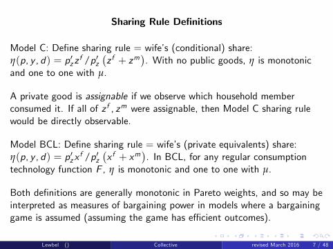
Sharing Rule Definitions

Model C: Define sharing rule = wife’s (conditional) share:η(p, y , d) = p′zz

f /p′z(z f + zm

). With no public goods, η is monotonic

and one to one with µ.

A private good is assignable if we observe which household memberconsumed it. If all of z f , zm were assignable, then Model C sharing rulewould be directly observable.

Model BCL: Define sharing rule = wife’s (private equivalents) share:η(p, y , d) = p′zx

f /p′z(x f + xm

). In BCL, for any regular consumption

technology function F , η is monotonic and one to one with µ.

Both definitions are generally monotonic in Pareto weights, and so may beinterpreted as measures of bargaining power in models where a bargaininggame is assumed (assuming the game has effi cient outcomes).


Earlier Sharing Rule Identification Results

Main identification result (early forms Chiappori 1992, Chiappori, Blundell,Meghir 2002, general form: Chiappori and Ekeland 2009): In model C withor without public goods, given just the household demand functionz = z (p, y , d), resource share levels η(p, y , d) are not identified, butderivatives of η(p, y , d) are (generically) identified

Application/variant of this result: Lechene and Attanasio (2010) see acash transfer to households that leaves food shares unchanged. Transferchanges y but could also be a d . Infer ∂η/∂d must be nonzero to offsettransfer’s effect through y on shares.

Without further assumptions, is also true for BCL that η(p, y , d) is notidentified, since not identified in the purely private goods model, which is aspecial case of both BCL and C.

Problem: many welfare/policy calculations depend on identifying η, not onjust ∂η/∂d , e.g., poverty rates, inequality measures, indifference scales.


Goal - Identify Sharing Rule Levels η, not just ∂η/∂d

Alternative methods for identifying η:

1. Collect extensive intrahousehold (assignable) consumption data:Cherchye, De Rock and Vermeulen (2010), Menon, Pendakur, Perali(2012). Can’t deal with sharing and externalities.

2. Obtain bounds on shares: Cherchye, De Rock and Vermeulen (2011),Cherchye, De Rock, Lewbel and Vermeulen (2013).

3. Restrict individual preferences across households of differentcompositions: Browning Chiappori Lewbel (BCL 2002, 2013), Couprie(2007), Lewbel and Pendakur (LP 2008), Bargain and Donni (2009,2012), Couprie, Peluso and Trannoy (2010), Lise and Seitz (2011).

4. Restrict sharing rules, assume preference similarities: Dunbar, Lewbel,and Pendakur (DLP 2013).

5. Restrict sharing rules and use distribution factors: Dunbar, Lewbel, andPendakur (DLP 2016).


Bounds

Naive bounds: a lower bound on each individual j ′s resource share is costof j ′s private, assignable consumption divided by total householdconsumption. We can do better.

Drop distribution factors d for now. Suppose we could see purchasedbundles z j1,...,z

jn of an individual j living alone in price/income regimes

p1/y1,...,pn/yn.

If j maximizes utility, then these bundles would satisfy revealed preferenceinequalities derived from Samuelson (1938), Houthakker (1950), Afriat(1967), Diewert (1973), and Varian (1982).

For a known vector valued function M j , write all these inequalities as

0 ≤ M j(z ji , pi/yii=1,...,n

)


Bounds continued

A single consumer j satisfies 0 ≤ M j(z ji , pi/yii=1,...,n

).

Assume model C (leave out public goods for now), and we observe acouple purchase bundles z1,...,zn in regimes p1/y1,...,pn/yn.Then theremust exist z f1 ,...,z

fn such that resource shares η1,...ηn satisfy inequalities

0 ≤ M f(z fi , pi/ηiyii=1,...,n

), 0 ≤ z fi ≤ zi ,

0 ≤ Mm(zi − z fi , pi/ (1− ηi ) yii=1,...,n

).

Min and max η1,...ηn over all possible zf1 ,...,z

fn that satisfy these

inequalities to get bounds on resource shares η1,...ηn.


Bounds continued

Extension 1: Include public goods and externalities. Can get informativebounds even if we do not know which goods are private and which arepublic, and which have externalities.

Extension 2: Observe/estimate couple’s demand functions z = z (p, y).Then can obtain inequalities for every possible p/y point to get tighterbounds.

Extension 3: Browning and Chiappori (1998) show SR1 (symmetry plusrank one) is the restriction on a couple’s demand system implied by Paretoeffi ciency. Can estimate z = z (p, y) imposing SR1 to further tightenbounds.

Note: We base bounds on WARP (weak axiom of revealed preference)inequalities applied to each household member. Imposing SARP may benumerically infeasible.


Bounds - Empirical Results

Some empirical results from Cherchye, De Rock, Lewbel and Vermeulen(2013). 865 childless working couples with full reporting, from 1999-2009US PSID. Goods are each spouse’s leisure (assumed private andassignable), food, housing, and other (allowed to have both public andprivate components and externalities).

Naive: Lower bound is own leisure only, upper is all expenditure exceptspouse’s leisure.

RP1: Reveled preference bounds from nonparametrically estimatedcouple’s demand system.

RP2: Bounds from parametric (QUAIDS) demand system with no utilityrestrictions imposed.

RP3: Bounds applied to parametric (QUAIDS) system with SR1restrictions imposed.


Bounds - Empirical Results

Naive: lower is leisure only, upper is all expenditure except spouse’s leisure.

RP1: nonparametrically estimated couple’s demand system.

RP2: parametric demands with no utility restrictions.

RP3: parametric demands with SR1 restrictions imposed.

Naive bounds RP1 bounds RP2 bounds RP3 boundsMean 17.52 11.33 9.72 3.44

First quartile 12.12 6.54 3.93 1.49Median 15.78 11.67 8.91 2.78

Third quartile 21.68 15.13 14.53 4.74

Table: Percentage point differences between upper and lower bounds on thefemale relative income share


BCL Model

Drop distribution factors d , not needed.

BCL demands z = h (p/y) obtained from

maxx f ,xm ,z

µ(p/y)U f (x f ) + Um(xm) such that z = F(x f + xm

), p′z = y

For j = f ,m, define x j = hj (p/y) as demands frommaxx j U j (x j ) | px j = y.

Define indirect utility functions V j (p/y) = U j[hj (p/y)

].


Working Towards Identification - Duality

BCL show duality: A shadow (Lindahl) price vector π(p/y) and a sharingrule 0 < η(p/y) < 1 exist such that

x f (py) = hf [π/ (ηy)] , xm(

py) = hm [π/ ((1− η) y)] , h(

py) = F

(hf + hm

)f maximizes her utility by buying xf = hf [π/ (ηy)] at shadow prices πwith share η of y . m does same with share 1− η. Adds up to householdbuying bundle z = F

(x f + xm

).

Pareto weight µ connected to resource share η by

µ = −[∂V f (π/ (ηy))/∂η

]/∂Vm [π/((1− η) y ]/∂η

So: given demands h, hf , hm , if π and η are identified, everything(ordinal) is identified.

Questions:1. How to identify demand functions h, hf , hm?2. Given h, hf , hm , are π, η identified? Address this first.


BCL - Generic Point Identification

Claim: If functions h, hf , hm known, then functions xm , x f , F , and η are"generically" identified (generic as in Chiappori and Ekeland 2009).

Proof sketch: let ρ = p/y . h, hf , hm known. Given any F ∈ ΩF , let

π(ρ) =DF (x)′.ρ

x ′DF (x)′.ρ, evaluated at x = F

−1[h(ρ)],

x(ρ, η) = hm [π(ρ)/(1− η)] + hf [π(ρ)/η],

η(ρ) = arg minη∗∈[0,1]

max |x(ρ, η∗)− F−1[h(ρ)]|.

and define F by F [x(ρ, η(ρ))] = h (ρ). This defines a mappingF = T

(F). True F is fixed point, and true η is η with F = F .

T might not be a contraction mapping. Loosely, existence of T showsenough demand functions are identified to generally permit recovery of Fand η; are identified as long as the demand functions are not too simple.


BCL - Linear Consumption Technology

Assume a linear consumption technology: z = F (x) = Ax + amakes shadow prices not depend on indirect utility functions:

π(p/y)y

=A′p

y − a′p

gives household demand functions the form:

z = h (p/y) = Ahf(

π(p/y)η(p/y)y

)+ Ahm

(π(p/y)

(1− η(p/y)) y

)+ a

= Ahf(

A′py − a′p

1η( py )

)+ Ahm

(A′p

y − a′p1

1− η( py )

)+ a


Linear Consumption Technology - Compare BCL to Gorman

BCL with linear consumption technology F is

z = h (p/y) = Ahf(

A′py − a′p

1η( py )

)+ Ahm

(A′p

y − a′p1

1− η( py )

)+ a

Gorman (1976) general linear technology household demand model is:

z = Ahm(

A′py − a′p

)+ a

Barten (1964) is Gorman’s model with a = 0 and A a diagonal matrix.

Gorman had similar motivation for consumption technology as a model ofsharing and jointness of consumption, but only in a unitary model.Gorman makes household demands be a scaled function of one individual’sdemands.

Gorman differs from BCL even if members all have same preferences(hf = hm) and same equivalent incomes (η = 1/2).


Nonparametric Identification With Linear Technology

Claim: Given observable demand functions, the functions xm , x f , F , and ηare generically identified if number of goods is n ≥ 3.

Take T ≥ n+ 10 price vectors p1, ..., pT . Then

z t = Ahf(

A′pt

y − a′pt1ηt

)+ Ahm

(A′pt

y − a′pt1

1− ηt

)+ a

For each t have (n− 1) independent equations, total (n− 1)T equations.The unknowns are A, a, and ηt ; total n2 + n+ T unknowns. With n ≥ 3and T ≥ n+ 10, have more equations than unknowns, so we haveidentification as long as the equations are linearly independent (not toosimple).

Examples: Identification fails for LES h, Scaling of Barten Technology Anot identified for homothetic hi .


Example: Identification In Almost Ideal Demand System

Claim: Assume hi is defined by budget sharesωi (p/y i ) = αi + Γi ln p + βi

[ln(y i)− c i (p)

]for i = m, f . Assume

βf 6= βm and elements of βf , βm , and the diagonal of A are nonzero.Then the functions xm , x f , F , and η are identified.

Actually substantially overidentifed. Most parameters are identified fromdemands on just one good. Models that nest Almost Ideal like QUAIDSare also identified.

Proof sketch: Have π = A′p/(1− a′p) and

zk = ak +∑jAkj

[η

πjωf(

π

ηy

)+1− η

πjωm

(π

(1− η)y

)]Intercepts identify a. Coeffi cients of ln y identify

∑j

[ηβfj + (1− η) βmj

]/ ∑`(A`j/Akj )p`. Variation in p and subscripts

identifies η, β coeffi cients and ratios A`j/Akj . Levels of Ajk are identified

from the quadratic price terms in ∑j Akj[

ηπjc f (π) + 1−η

πjcm (π)

].


Identifying Demand Functions

z = h (p/y) are household demand functions obtained from

maxx f ,xm ,z

µ(p/y)U f (x f ) + Um(xm) | z = F(x f + xm

), p′z = y

h (p/y) identified from data on a household’s purchases in many p/yregimes. More commonly, estimated from data on many household’spurchases, assuming preferences are identical up to observable covariatesand ignorable errors. Later we’ll introduce unobserved heterogeneity intothe model.

The diffi culty is not identifying household’s demand functionsz = h (p/y), rather, it is identifying individual household member’sdemand functions x j = hj (p/y) that come from maxx j U j (x j ) | px j = y.


Methods of Identifying Household Member’s Demand Functions

Overly strong BCL Identify hj (p/y) from data on purchases by singlesliving alone.

How to weaken this assumption?

Model how individual’s preferences change when they marry (not done).

Impose constraints on π, η to weaken data requirements on h, hm , hf .Examples: π linear or Barten, η independent of y (at some y levels).

Impose restrictions on how hm , hf vary across people (later SAP).

Impose restrictions on how hm , hf vary across households of differenttypes (later SAT).

Exploit combination of η independent of y with presence of distributionfactors.


Simplifying the Model

Assume Barten technology: a = 0, A diagonal. Letw k (y , p,A) = couple’s budget share of good k.w kj (y , p) = budget share of good k from utility function U j (x j ), j = m, f .

BCL model then becomes, in budget share form

w k (y , p,A) = ηw kf(ηy ,A′p

)+ (1− η)w km

((1− η) y ,A′p

)η = η(p, y ,A)

BCL estimate this model, with Quadratic Almost Ideal Demand SystemQUAIDS model (Banks, Blundell, and Lewbel 1997) for singles.


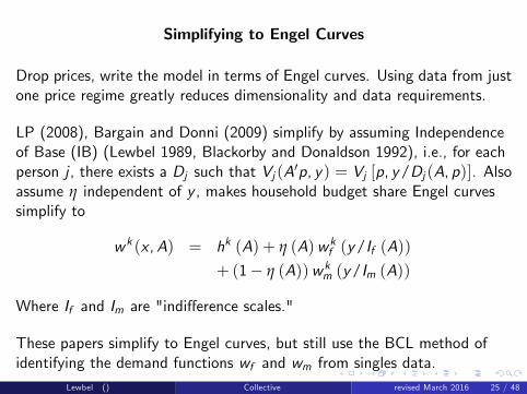
Simplifying to Engel Curves

Drop prices, write the model in terms of Engel curves. Using data from justone price regime greatly reduces dimensionality and data requirements.

LP (2008), Bargain and Donni (2009) simplify by assuming Independenceof Base (IB) (Lewbel 1989, Blackorby and Donaldson 1992), i.e., for eachperson j , there exists a Dj such that Vj (A′p, y) = Vj [p, y/Dj (A, p)]. Alsoassume η independent of y , makes household budget share Engel curvessimplify to

w k (x ,A) = hk (A) + η (A)w kf (y/If (A))+ (1− η (A))w km (y/Im (A))

Where If and Im are "indifference scales."

These papers simplify to Engel curves, but still use the BCL method ofidentifying the demand functions wf and wm from singles data.


Is η Independent of y reasonable?

Can resource shares η be independent of total expenditures y , as assumedby these "identification just from Engel curves" models? It generatestestable restrictions, see DLP (2013).

Empirical evidence Menon, Pendakur, Perali (2012); Cherchye, De Rock,Lewbel and Vermeulen (2013).

Permits η to depend on prices, incomes of each member, wealth,distribution factors, etc. Only assuming η independent of y afterconditioning on these other things.

Does not violate Samuelson (1956), who showed resource shares can’t beconstant for a large class of social welfare functions, since it permits sharesto depend on prices.

DLP (2013, online appendix) provides an example of a sensible class ofmodels of utility functions and Pareto weights that yield η independent ofy : PIGL or PIGLOG (Muellbauer 1976) utility with weighted S-Gini(Donaldson and Weymark 1980) household social welfare functions.

Some results (DLP 2013) only need independence at low levels y .Lewbel () Collective revised March 2016 26 / 48

Some Summary Empirical Results

Use the LP (2008) Engel curve simplification of BCL - singles and couplesdata. Four models (vary by demographics included and outlier handling).1990-92 Canadian Family Expenditure Survey, 12 consumption goods, 419single men, 450 single women, and 332 couples.

Estimated resource share η for median women: 0.36 to 0.46. Small ageand education effects (these affect both preferences and shares). Raisingproportion of household’s income she contributes up by .5 raises η byabout .05.

Other estimates: scale-economy measure p′z/p′x should lie between 1/2(full sharing) and 1 (completely private). Estimated range 0.70 to 0.78.Indifference scales for women If around 1.53; for men Im around 1.44. Aperson needs about two thirds, 1/1.53 or 1/1.44 of couple’s income toreach the same indifference curve living alone that one attains living with apartner.


Dropping the use of Singles data

Bounds don’t use singles data (does need prices). DLP (2013, 2016) getpoint identification without prices, without singles, and without the IBassumption. They use Engel curves, assume a private assignable good foreach household member.

Further simplify estimation (and further relax data requirements andmodeling constraints) by only using data on the one private assignablegood for each household member, and without price data.

To maintain identification, keep the assumption that resource shares η areindependent of total expenditures y (at least for low levels of y). Inaddition:

DLP (2013) Add SAP or SAT restrictions on demand functions, or,

DLP (2016) make use of distribution factors.


Focus on Assignable Goods, Bring in Children

Have s children, impose same utility function for each. Household does

maxU[U f (x f ),Um(xm),Uc (xc ), p/y , s

]| z = F

(x f + xm + sx s , s

), p′z = y

Looking only at private assignable goods (say, clothing), household’sbudget shares are given by

Wcs (y) = sηcswcs (ηcsy) , Wms (y) = ηmswms (ηmsy) ,

Wfs (y) = ηfswfs (ηfsy) .

Wfs (y) = fraction of y household spends on woman’s clothes in a singleprice regime p. These can be estimated.

wcs (y) = fraction of y spent that would be spent on woman’s clothesdetermined by maxU f (x f ) | π′sz = y, at shadow prices πs given byBarten technology for household with s children.

ηfs = woman’s resource share in house with s children.

Similar for man m and child c .Lewbel () Collective revised March 2016 29 / 48

Identification Strategies

Wcs (y) = sηcswcs (ηcsy) , Wms (y) = ηmswms (ηmsy) ,

Wfs (y) = ηfswfs (ηfsy) .

We observe W functions, want to identify resource shares η.

LP (2008), Bargain and Donni (2009), extend BCL method by learningfunctions wms (y) and wfs (y) from data on singles.

DLP (2013), place semiparametric restrictions (SAP) or (SAT) on thefunctions wms (y), wfs (y), and wcs (y). Not restrictions on shape, butrestrictions that make some feature of these functions be similar acrosspeople (SAP) or similar across household size/types (SAT).

DLP (2016), combine η not depending on y with distribution factors.


Similar Across People SAP Identification

SAP demand: wj (y , p) = hj (p) + g(

yGj (p)

, p)for y ≤ y ∗, j = m, f , c .

Functions hj , Gj , and g can be anything, but g is the same across people.

Paper gives SAP class of utility functions. SAP, which is similar to butweaker than shape invariance, need apply only to the assignable goods(clothing). Get

Wcs (y) = αcs + sηcs gs (ηcsγcsy) ,

Wms (y) = αms + ηms gs (ηmsγmsy)

Wfs (y) = αfs + ηfs gs (ηfsγfsy)

Note γjs = Gj (πs (p)), shadow prices depend on household type/size s,which makes these functions vary by s in the Engle curves. Same forαjs = hj (πs (p)) and gs (·) = g (·,πs (p)).


Similar Across People SAP Identification

SAP Identification overview: By SAP we have

Wcs (y) = αcs + sηcs gs (ηcsγcsy) ,

Wms (y) = αms + ηms gs (ηmsγmsy)

Wfs (y) = αfs + ηfs gs (ηfsγfsy)

Look at derivatives with respect to y at y = 0:

W ′fs (0) = γfsη2fs g′s (0) , W ′′fs (0) = γ2fsη

3fs g′′s (0) ,

W ′′′fs (0) = γ3fsη4fs g′′′s (0)

and same for m and c . Along with ηfs + ηms + sηcs = 1 gives 10equations in 9 unknowns ηfs , ηms , ηcs , γfs , γms ,γcs , g

′s (0), g

′′s (0), and

g ′′′s (0), for each household size s.

Identification only used derivatives at y = 0, so only needed restrictions tohold for small y .


Similar Across Types Identification

SAT demand: wj (y , p) = gj(

yGt (p)

, p)for y ≤ y ∗, j = m, f , c , where p

are prices only of private goods. Functions hj , Gj , and gj can be anything,but the g function only depends on prices through p.

Again only need to hold for clothing. Get

Wcs (y) = αcs + sηcs gc (ηcsγcsy)

Wms (y) = αms + ηms gm (ηmsγmsy)

Wfs (y) = αfs + ηfs gc (ηfsγfsy)

SAP made gs (·) = g (·,πs (p)) only have a type s subscript, while SATmakes gj (·) = gj (·, p) only have a person j subscript.

For identification, look at same derivatives as in SAP, but now combineacross a households of a few different types (difference sizes s), using thatgj (0) doesn’t vary by s, to get more equations than unknowns.


Some Estimates Using SAP or SAT - Malawi Data

The Malawi Integrated Household Survey, conducted in 2004-2005. fromthe National Statistics Offi ce of the Government of Malawi with assistancefrom the International Food Policy Research Institute and the World Bank.

High quality data: enumerators were monitored; big cash bonuses wereused as an incentive system; about 5 per cent of the original randomsample in each year had to be resampled because dwellings wereunoccupied; (only) 0.4 per cent of initial respondents refused to answerthe survey.

We use 2794 households comprised of non-urban married couples with 1-4children aged less than 15. Private assignable good is men’s, women’s andchildren’s clothing (including footwear).

Demographics: region, children age summaries, fraction of girls, adult lowand high age dummies, education levels of each spouse, distance to a roadand to a market, dry season dummy, religion (christian, muslim,animist/other).


Estimated Levels of Resource SharesSAP SAT SAP&SAT

Est Std Err Est Std Err Est StdErr1 kid man 0.443 0.048 0.378 0.076 0.400 0.045

woman 0.308 0.041 0.368 0.062 0.373 0.042kids 0.249 0.037 0.254 0.072 0.227 0.036

each kid 0.249 0.037 0.254 0.072 0.227 0.0362 kids man 0.423 0.051 0.436 0.090 0.462 0.051

woman 0.222 0.042 0.212 0.056 0.221 0.043kids 0.355 0.045 0.352 0.100 0.317 0.045

each kid 0.177 0.022 0.176 0.050 0.158 0.0233 kids man 0.427 0.057 0.437 0.099 0.466 0.053

woman 0.185 0.046 0.166 0.054 0.176 0.044kids 0.388 0.050 0.397 0.114 0.358 0.050

each kid 0.129 0.017 0.132 0.038 0.119 0.0174 kids man 0.318 0.070 0.352 0.112 0.384 0.063

woman 0.214 0.054 0.168 0.062 0.182 0.052kids 0.468 0.061 0.479 0.133 0.434 0.059

each kid 0.117 0.015 0.120 0.033 0.109 0.015Lewbel () Collective revised March 2016 35 / 48

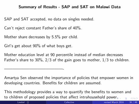
Summary of Results - SAP and SAT on Malawi Data

SAP and SAT accepted, no data on singles needed.

Can’t reject constant Father’s share of 40%.

Mother share decreases by 5.5% per child.

Girl’s get about 90% of what boys get.

Mother education level at 90 percentile instead of median decreasesFather’s share to 30%, 2/3 of the gain goes to mother, 1/3 to children.

– – – – – – – – – – – – – – -

Amartya Sen observed the importance of policies that empower women indeveloping countries. Benefits for children are assumed.

This methodology provides a way to quantify the benefits to women andto children of proposed policies that affect intrahousehold power.


Another SAP and SAT application - Missing Women in India

Anderson and Ray (2010) estimate that in India, 1.7 million woman overage 45 “missing:”died at younger than expected ages.The number missing increases with age from 45 to 70.No good theory why. Poverty kills, but household poverty rates do notcorrelate with women’s age.

Calvi, R. (2016), "Why Are Older Women Missing in India? The AgeProfile of Bargaining Power and Poverty" Boston College Working paper.


Another SAP and SAT application - Missing Women in India -continued

Calvi first looks at a an inheritence law that increases women’s bargainingpower.Changes in the law varied by state, time, and religious affi liation.Finds corresponding improvements in health outcomes where and whenthe law changed.

Calvi then uses SAP and SAT to estimate women’s resource shares. Findsthey decrease with age after 45.Use the shares and household income to calculates the ratio of women inpoverty to men in poverty by age.The correlation of estimated poverty ratio to Anderson and Ray’s estimateof missing women is amazing: .96


Point Identification by Distribution Factors

DLP (2016): No preference restrictions. η depends on distribution factorsd , not on y , we have

Wcs (y , d) = sηcs (d)wcs [ηcs (d) y ]

Wms (y , d) = ηms (d)wms [ηms (d) y ]

Wfs (y , d) = ηfs (d)wfs [ηfs (d) y ] .

We observe W functions, want to identify resource shares η.

Identification (intuition, real proof doesn’t need y = 0): Again look atderivatives wrt y at y = 0:

W ′fs (0) = [ηfs (d)]2 w ′fs (0)

and similar for m and c . For each value d takes on, this along withsηcs (d) + ηms (d) + ηcs (d) = 1 gives 4 equations. If d takes on at least3 different values then we get 12 equation in the 12 unknowns w ′cs (0),w ′ms (0), w

′fs (0), and, for each of 3 values of d , ηcs (d), ηms (d), and

ηcs (d).Lewbel () Collective revised March 2016 39 / 48

Unobserved Distribution Factors

It’s unrealistic to think we can observe all or even most of what affectshousehold’s resource distributions.

Suggests modeling resource shares as random variables.

Will also want to consider individual preferences varying across households(random utility parameters).

Chiappori and Kim (2013): have random resource shares, don’t identifylevels of shares.

DLP (2016): Assume resource shares conditionally independent of y ,distribution factors that can take on 3 values, private assignables that arenormal goods, differentiable in y . Then the entire joint distributionfunction of random resource shares ηcs , ηms , and ηcs is identified.


DLP (2016): Assume resource shares conditionally independent of y ,distribution factors that can take on 3 values, private assignables that arenormal goods, differentiable in y . Then the entire joint distributionfunction of random resource shares ηcs , ηms , and ηcs is identified.

Proof sketch: Look in expenditures form Yfs = yWfs = ψfs (ηfsy). HaveFYfs (ω | y) = Pr (Yfs ≤ ω | y) = Pr (ψfs [ηfsy ] ≤ ω | y)= Pr

(ηfs ≤

ψ−1fs (ω)y | y

)= Fηfs

(ψ−1fs (ω)y | y

)= Fηfs

(ψ−1fs (ω)y

). So

exp(∫ y ∂FYfs (ω|y )/∂ω

∂FYfs (ω|y )/∂y dω)= exp

(∫ ∂ ln ψ−1fs (ω)∂ω dω

)= ψ−1fs (ω) κfs where

unknown κfs is exponential of the constant of integration. So ψ−1fs isidentified up to κfs , similar for other household members. Sinceψ−1fs (ω) = ηfsy , this shows we can identify the joint distribution ofηfs/κfs , ηms/κms , ηcs/κcs . Apply previous identification by distributionfactors to the means of these distributions to identify κfs , κms , and κcs , sothen entire joint distribution of ηfs , ηms , ηcs is identified.Extension: Show can identify both random resource shares and a randomutility (preference) parameter.


Other Welfare Calculations - Equivalence Scales vs IndifferenceScales

An equivalence scale E f is the fraction of a household’s income anindividual woman f living alone needs to attain the same utility level asthe household. Given indirect utility functions V f for the woman, andhousehold indirect utility function V , Equivalence scale E f solves:

V f(pE f y

)= V

(py

)Problem: Traditional Equivalence scales are fundamentally not identifiable.For any monotonic G , (relabeling the woman’s indifference curves) get adifferent E f from the observationally equivalent equation

G[V f(pE f y

)]= V f

(pE f y

)= V

(py

)Also, household may use a bargaining model that does not correspond toexistence of a well defined household utility function V .


A replacement for Equivalence Scales: Indifference Scales

BCL define an Indifference scale I f as the fraction of the household’sincome that woman f living alone would need to attain the sameindifference curve over goods that she had as a member of the household.

Given indirect utility function V f for f , household shadow prices π fromsharing and woman’s resource share η, I f solves:

V f(pI f y

)= V f

(π

ηy

)Unaffected by monotonic transformations of utility. Replacing V f (·) withG[V f (·)

]leaves I f unchanged.

Indifference scale don’t require existence of a household utility function V ,avoids issues of interpersonal comparability and differences in indifferencecurves, and is identified from revealed preference data given identificationof π and η.


Constructing Indifference Scales

V f (p/y f ) is indirect utility of f . Apply Roy’s to get demands hf (p/y f ).

In the household, f consumes equivalent bundle x f = hf (π/ (ηy)), sameas if she were living alone and facing prices/income = π/ (ηy).

The indifference scale is I f (p, y) defined by

V f(

pI f (p, y)y

)= V f

(π(p/y)η(p/y)y

)So I f (p, y)y is income that would be required by f living alone to attainsame indifference curve over goods that f attains in the couple, consumingbundle x f = hf (π/η).

I f (p, y) is fully identified and ordinal, not affected by choice ofcardinalization for V f .

Construct same for m, replacing f with m and η with 1− η.Lewbel () Collective revised March 2016 44 / 48

Example Uses for Indifference Scales

If a couple has income y and husband dies, surviving f will need incomep′hf (π/ (ηy)) to buy the same bundle she consumed before, or I f y to beon the same indifference curve for goods as before (excludes loss of utilityfrom companionship). Use for wrongful death lawsuits, life insurance,alimony.

I f y = fraction of a couple’s income that a women living alone needs to beas well off as she’d be in the couple. Use for welfare comparisons.

Given singles poverty lines y f , ym , couple’s poverty line is y is theminimum value of y such that an η exist satisfying the inequalities

V f(py f

)≤ V f

(π (p/y)

ηy

),Vm

(pym

)≤ Vm

(π (p/y)(1− η) y

)


More Example Uses for Indifference Scales

Ratio I f /Im compares single’s income requirements by looking at howmuch each needs alone to be as well off as they would be in the samehousehold. I f /Im might not equal one even if f and m have samepreferences, because of bargaining η.

If we know woman’s outside option, i.e., the income y f , she would have iflived alone, we can calculate how big her share η would need to be tomake her better off, in terms of goods consumption, in the household.Could be used for threat point bargaining calculations. This η solves

V f(py f

)= V f

(π(p/y)

η(p, y , y f )y

)The model separately identifies tastes, bargaining, and sharing.


Conclusions - 1

Resource shares are a better measure of household resource allocation andpower than Pareto weights (do not depend on a cardinalization of utility).

Many household welfare calculations depend on resource share levels, notjust how they vary with distribution factors.

A variety of alternative identifying strategies are proposed to point identifyor to bound resource shares.

Most recently, these include identifying distribution of resource sharesacross households allowing for unobserved distribution factors (unobservedvariation in power) and unobserved hetereogeneity in preferences.


Conclusions - 2

Among point identification strategies, most attractive may be: assume oneprivate assignable good per individual type, resource shares independent oftotal expenditures, and an observable distribution factor. This permitscomplete identification of the joint distribution of random resource shares,with almost no restrictions on preferences, from just private goods demandfunctions, even without price variation.

An example of a welfare calculation based on resource sharing is thecalculation of indifference scales. Unlike equivalence scales, indifferencescales can be identified by revealed preference.

Other useful welfare calculations include bargaining power measures,measuring poverty rates for individuals (including children), extendingregional inequality measures to the level of individuals instead ofhouseholds, and measuring economies of scale arising from jointness ofconsumption.


Documents

an overview Arthur Lewbel Boston College revised · PDF filean overview Arthur Lewbel Boston College revised March 2016 ... 1981). Assume Pareto e¢ cient households (rules ... (leave