Embed Size (px)
Citation preview
An Overview of Automatic Differentiation and Introduction to the OpenAD/F Tool
Paul Hovland, Jean Utke
Mathematics & Computer Science DivisionArgonne National Laboratory
Argonne Automatic Differentiation Group Members
Paul HovlandAndrew Lyons (UChicago)Sri Hari Krishna Narayanan (starts 11/08)Boyana NorrisIlya SafroJaewook ShinJean Utke (joint w/ UChicago)
Alumni: J. Abate, C. Bischof, S. Bhowmick, A. Griewank, P. Khademi, J. Kim, P. Malusare, U. Naumann, L. Roh, M. Strout, B. Winnicka
Funding
Current:– DOE: Applied Mathematics Base Program– DOE: Computer Science Base Program– DOE: CSCAPES SciDAC Institute– NASA: ECCO-II Consortium– NSF: Collaborations in Math & Geoscience
Past:– DOE: Applied Math– NASA Langley– NSF: ITR
Outline
Introduction to automatic differentiation (AD)AD in nuclear systems modelingComputing derivatives efficiently under various scenariosIdeas for computing very large, very dense Jacobians efficientlySurvey of available toolsApplication examplesHandoff to Utke for discussion of OpenAD/F and its application to SCALE

Automatic Differentiation in a Nutshell
Technique for computing analytic derivatives of programs (millions of loc)Derivatives used in optimization, sensitivity analysis, inverse problems, …AD = analytic differentiation of elementary functions + propagation by chain rule– Every programming language provides a limited number of
elementary mathematical functions– Thus, every function computed by a program may be viewed as the
composition of these so-called intrinsic functions– Derivatives for the intrinsic functions are known and can be combined
using the chain rule of differential calculusAssociativity of the chain rule leads to two main modes: forward and reverse (adjoint)Can be implemented using source transformation or operator overloading
Automatic Differentiation in Nuclear System Modeling
Derivatives used for:– Local sensitivity analysis– Construction of first- and second-order Taylor models– Providing weights for adaptive sampling– Other applications??
What is feasible & practical– Jacobians of functions with small number (1—1000) of independent
variables (forward mode)– Jacobians of functions with small number (1—100) of dependent
variables (adjoint mode)– Very (extremely) large, but (very) sparse Jacobians and Hessians
(forward mode plus coloring)– Jacobian-vector products (forward mode)– Transposed-Jacobian-vector products (adjoint mode)– Hessian-vector products (forward + adjoint modes)
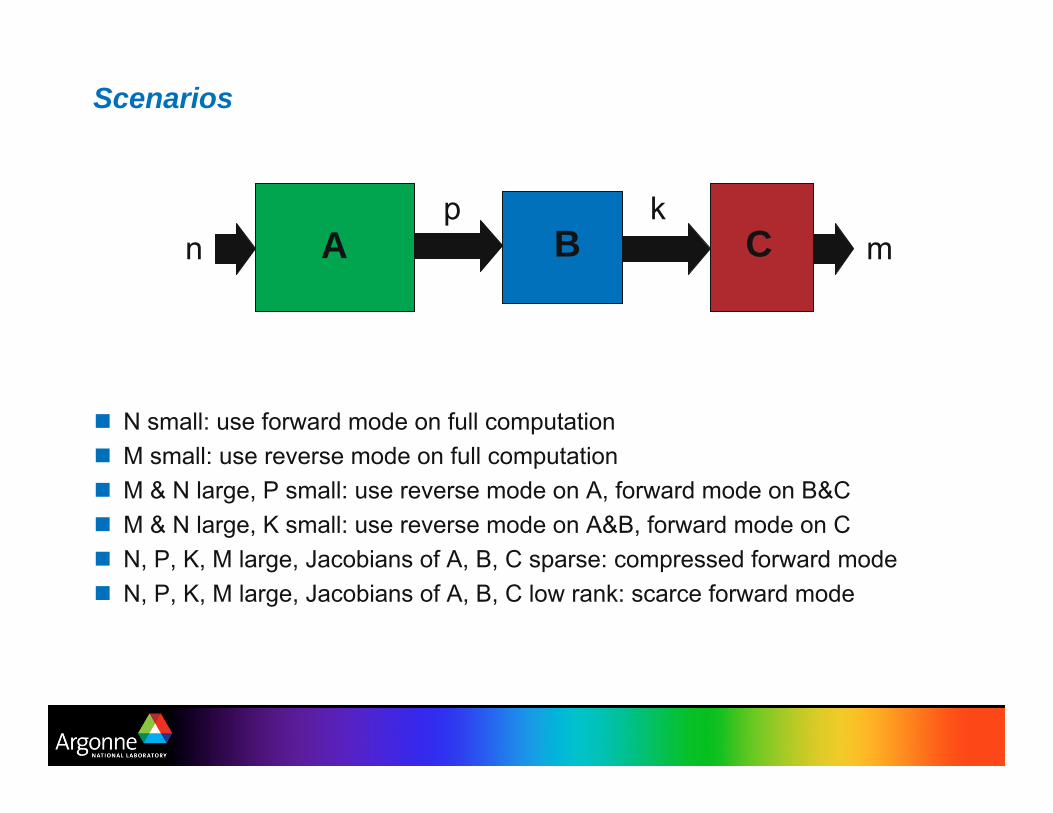
Scenarios
N small: use forward mode on full computationM small: use reverse mode on full computationM & N large, P small: use reverse mode on A, forward mode on B&CM & N large, K small: use reverse mode on A&B, forward mode on CN, P, K, M large, Jacobians of A, B, C sparse: compressed forward modeN, P, K, M large, Jacobians of A, B, C low rank: scarce forward mode
np k
mA B C
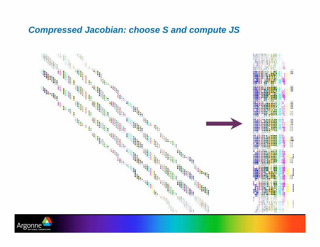
Compressed Jacobian: choose S and compute JS

Matrix Coloring (used to determine S)
1 2 0 0 50 0 3 0 00 2 3 4 01 0 0 0 00 0 0 4 5
1 2 0 0 50 0 3 0 00 2 3 4 01 0 0 0 00 0 0 4 5
1 2 0 0 50 0 3 0 00 2 3 4 01 0 0 0 00 0 0 4 5
1 2 0 53 0 0 03 2 4 01 0 0 00 0 4 5
1 2 50 0 34 2 31 0 04 0 5
1 2
3
4
5
1 2
3
4
5
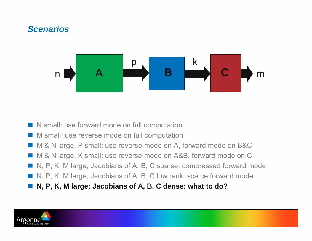
Scenarios
N small: use forward mode on full computationM small: use reverse mode on full computationM & N large, P small: use reverse mode on A, forward mode on B&CM & N large, K small: use reverse mode on A&B, forward mode on CN, P, K, M large, Jacobians of A, B, C sparse: compressed forward modeN, P, K, M large, Jacobians of A, B, C low rank: scarce forward modeN, P, K, M large: Jacobians of A, B, C dense: what to do?
np k
mA B C
What to do for very large, dense Jacobian matrices?
Jacobian matrix might be large and dense, but “effectively sparse”– Many entries below some threshold ε (“almost zero”)– Can tolerate errors up to δ in entries greater than ε– Example: advection-diffusion for finite time step: nonlocal terms fall
off exponentially– Solution: do a partial coloring to compress this dense Jacobian:
requires solving a modified graph coloring problemJacobian might be large and dense, but “effectively low rank”– Can be well approximated by a low rank matrix– Jacobian-vector products (and JTv) are cheap– Adapt techniques based on sampling of F or finite difference
approximations to Jv, [F(x+hv) – F(x)]/h– One candidate: SVD of random Jacobian-vector products (adaptation
of efficient subspace method--joint work with Abdel-Khalik)

Tools
Fortran 95C/C++Fortran 77MATLAB
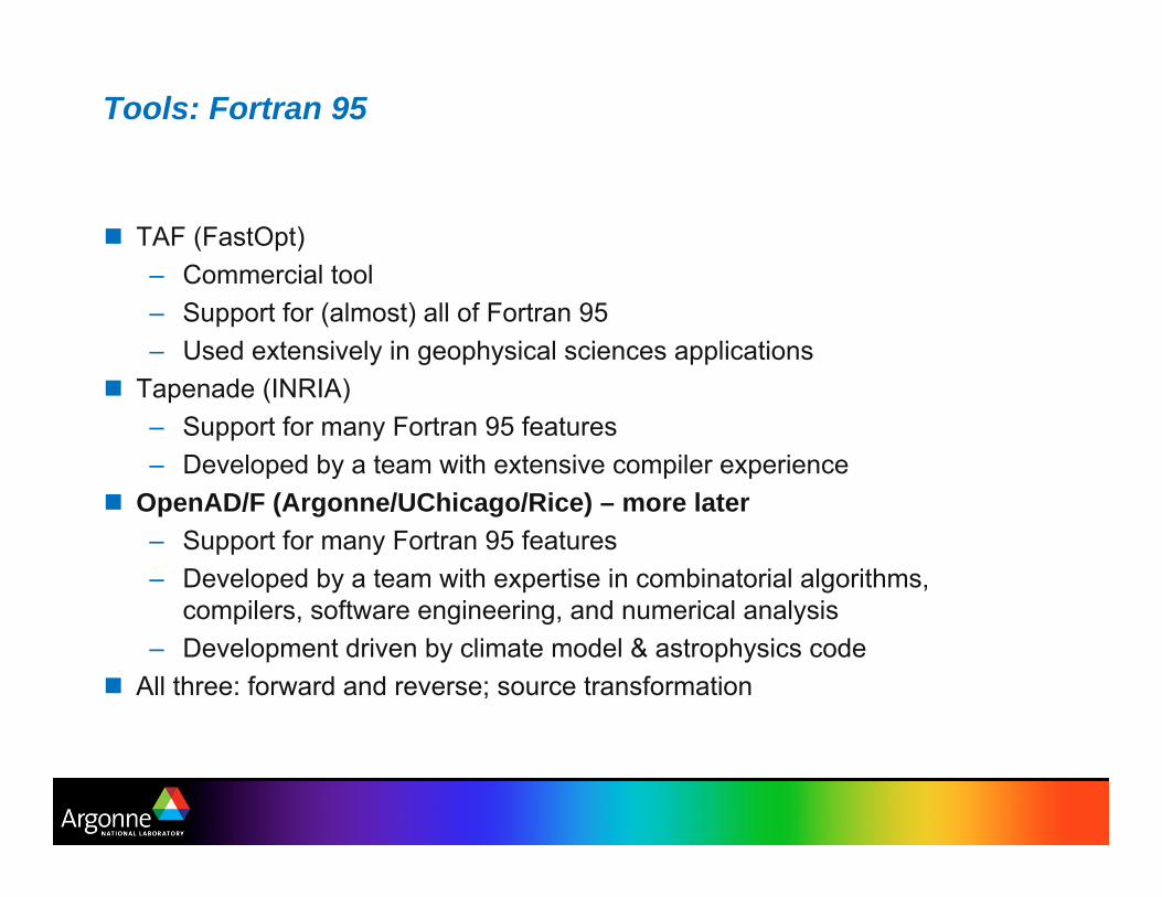
Tools: Fortran 95
TAF (FastOpt)– Commercial tool– Support for (almost) all of Fortran 95– Used extensively in geophysical sciences applications
Tapenade (INRIA)– Support for many Fortran 95 features– Developed by a team with extensive compiler experience
OpenAD/F (Argonne/UChicago/Rice) – more later– Support for many Fortran 95 features– Developed by a team with expertise in combinatorial algorithms,
compilers, software engineering, and numerical analysis– Development driven by climate model & astrophysics code
All three: forward and reverse; source transformation
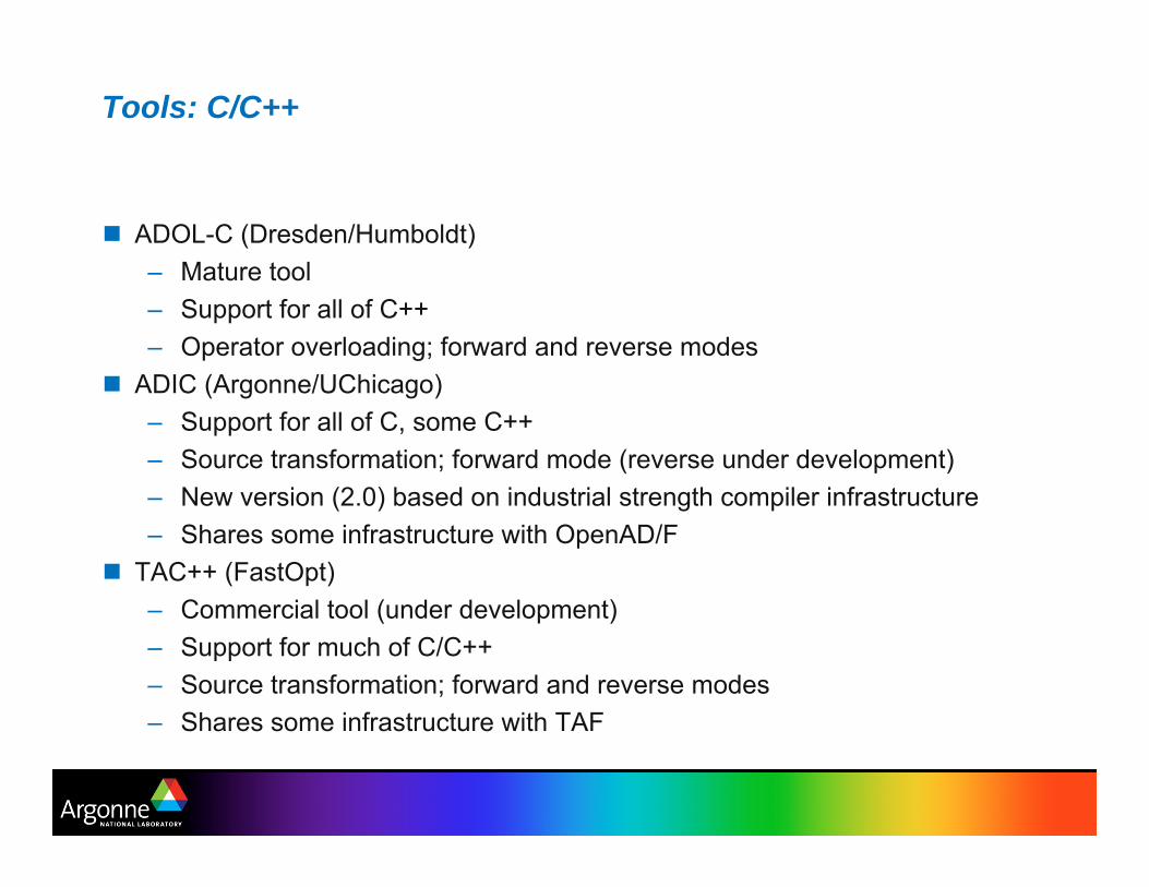
Tools: C/C++
ADOL-C (Dresden/Humboldt)– Mature tool– Support for all of C++– Operator overloading; forward and reverse modes
ADIC (Argonne/UChicago)– Support for all of C, some C++– Source transformation; forward mode (reverse under development)– New version (2.0) based on industrial strength compiler infrastructure– Shares some infrastructure with OpenAD/F
TAC++ (FastOpt)– Commercial tool (under development)– Support for much of C/C++– Source transformation; forward and reverse modes– Shares some infrastructure with TAF
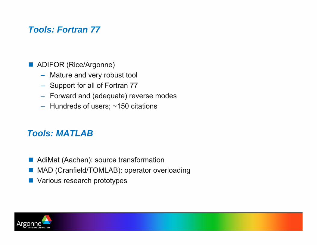
Tools: Fortran 77
ADIFOR (Rice/Argonne)– Mature and very robust tool– Support for all of Fortran 77– Forward and (adequate) reverse modes– Hundreds of users; ~150 citations
AdiMat (Aachen): source transformationMAD (Cranfield/TOMLAB): operator overloadingVarious research prototypes
Tools: MATLAB
Applications
Nonlinear solver (importance of analytic derivatives)Mesh smoothing (potential for automatic code to outperform hand coding)Simplified climate model (importance of reverse mode and compiler analysis)
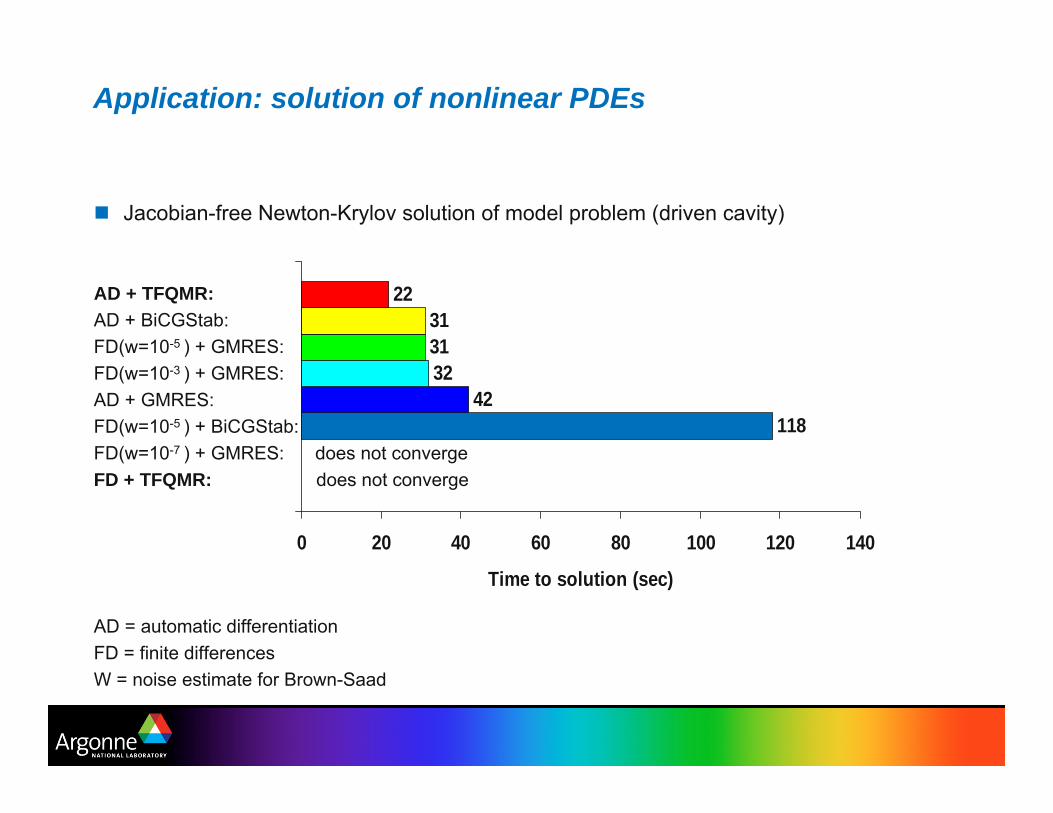
Application: solution of nonlinear PDEs
Jacobian-free Newton-Krylov solution of model problem (driven cavity)
AD + TFQMR:AD + BiCGStab:FD(w=10-5 ) + GMRES:FD(w=10-3 ) + GMRES:AD + GMRES:FD(w=10-5 ) + BiCGStab:FD(w=10-7 ) + GMRES: does not convergeFD + TFQMR: does not converge
AD = automatic differentiationFD = finite differencesW = noise estimate for Brown-Saad
11842
323131
22
0 20 40 60 80 100 120 140
Time to solution (sec)
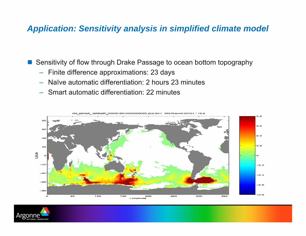
Application: Sensitivity analysis in simplified climate model
Sensitivity of flow through Drake Passage to ocean bottom topography– Finite difference approximations: 23 days– Naïve automatic differentiation: 2 hours 23 minutes– Smart automatic differentiation: 22 minutes
For More Information
Andreas Griewank, Evaluating Derivatives, SIAM, 2000.Griewank, “On Automatic Differentiation”; this and other technical reports available online at: http://www.mcs.anl.gov/autodiff/tech_reports.htmlAD in general: http://www.mcs.anl.gov/autodiff/, http://www.autodiff.org/ADIFOR: http://www.mcs.anl.gov/adifor/ADIC: http://www.mcs.anl.gov/adic/OpenAD: http://www.mcs.anl.gov/openad/Other tools: http://www.autodiff.org/E-mail: [email protected]