Embed Size (px)
Citation preview

JSS Journal of Statistical SoftwareAugust 2013, Volume 54, Issue 14. http://www.jstatsoft.org/
An R Package for Probabilistic Latent Feature
Analysis of Two-Way Two-Mode Frequencies
Michel MeuldersHUBrussel
Abstract
A common strategy for the analysis of object-attribute associations is to derive a low-dimensional spatial representation of objects and attributes which involves a compensatorymodel (e.g., principal components analysis) to explain the strength of object-attributeassociations. As an alternative, probabilistic latent feature models assume that objectsand attributes can be represented as a set of binary latent features and that the strengthof object-attribute associations can be explained as a non-compensatory (e.g., disjunctiveor conjunctive) mapping of latent features. In this paper, we describe the R package plfmwhich comprises functions for conducting both classical and Bayesian probabilistic latentfeature analysis with disjunctive or a conjunctive mapping rules. Print and summaryfunctions are included to summarize results on parameter estimation, model selectionand the goodness of fit of the models. As an example the functions of plfm are used toanalyze product-attribute data on the perception of car models, and situation-behaviorassociations on the situational determinants of anger-related behavior.
Keywords: latent feature, two-way two-mode data, disjunctive model, conjunctive model,perceptual mapping, EM algorithm, R.
1. Introduction
The analysis of a two-way frequency table is a basic task in data analysis which is of interestto researchers in various domains of applied research (Agresti 2002). Depending on the type ofdistribution which is appropriate for modelling the frequencies, one may distinguish betweenseveral types of frequency data. In particular, a multinomial distribution is appropriatefor modelling the frequencies in a two-way contingency table, and a Poisson distribution isappropriate for modelling frequencies which represent (unbounded) counts. Another type oftwo-way frequency data, which is the focus of the present paper, arises when the frequenciesare derived by aggregating three-way three-mode or two-way three-mode binary observations

2 Probabilistic Latent Feature Analysis in R
across the entities of one mode. In that case, a binomial distribution for modelling thefrequencies may be considered appropriate.
Both three-way three-mode and two-way three-mode binary data are of interest in severalsubstantive domains. First, three-way three-mode binary data occur when multiple ratersjudge for each of a set of objects and for each of a set of attributes whether or not a certainobject has a certain attribute. For instance, when investigating product perception in amarketing context, one may ask consumers to judge whether products have a certain attribute.In personality psychology, one may ask respondents to judge whether they would display aspecific behavior in a specific situation. In psychiatric diagnosis, one may ask several cliniciansto judge whether or not a certain patient has a certain symptom.
Second, two-way three-mode data occur when respondents nested in groups respond to aset of binary items. For instance, in the context of cross cultural research, respondents ofdifferent countries may respond to binary statements in a survey. In educational research,pupils nested in schools may complete an intelligence test that consists of binary items.
As fully modelling three-way three-mode or two-way three-mode binary data may be complex,researchers may start by analyzing the marginal two-way frequency table that is obtained byaggregating three-way three-mode data or two-way three-mode data across entities of onemode (i.e., raters or respondents).
More specifically, one may use a classical multivariate technique such as principal componentsanalysis (PCA) or correspondence analysis (CA) to derive a low-dimensional spatial repre-sentation of the row- and column elements, or exploratory factor analysis (EFA) to revealthe latent factor structure underlying the observed frequencies. Applying such a dimensionreduction or latent variable technique can be interesting in several applications: For instance,in a marketing context, a correspondence analysis of product-attribute frequencies can beused to derive a so-called perceptual map of products and attributes in a geometric space, thedimensions of which reflect the most important cognitive dimensions that drive product per-ception (Hoffman and Franke 1986; Torres and Bijmolt 2009). Furthermore, correspondenceanalysis and its extensions are a popular technique for ordination of species in vegetation sci-ence (Oksanen et al. 2012). Finally, in the context of document-retrieval conducting a PCA(or a two-mode factor analysis) on a term-by-document frequency matrix can help to revealthe semantic structure of a text (Deerwester, Dumais, Furnas, Landauer, and Harshman 1990;Landauer, Foltz, and Laham 1998).
PCA can be obtained by applying a singular value decomposition to the raw frequency table,or to the matrix of correlations or covariances between the columns. R functions for apply-ing PCA to the matrix of correlations or covariances are princomp() (R Core Team 2013),dudi.pca() in the package ade4 (Dray and Dufour 2007; Chessel, Dufour, and Thioulouse2004) and PCA() in the package FactoMineR (Le, Josse, and Husson 2008; Husson, Josse, Le,and Mazet 2012). R functions that apply singular value decomposition to the frequency tableare prcomp() (R Core Team 2013) and lsa() in the package lsa for latent semantic analysisof a term by document matrix of frequencies (Wild 2011).
EFA uses a latent variable approach to model the correlations between the column elementsby assuming that observed variables are a linear combination of a number of common latentfactors and a specific error term. EFA differs from applying PCA to the correlation matrixin that it only decomposes the common variance in terms of latent factors. To conduct EFAwith R one may use factanal() (R Core Team 2013).

Journal of Statistical Software 3
Correspondence analysis involves using a singular value decomposition to decompose the Chi-square statistic associated to the frequency table. R functions for applying correspondenceanalysis are corresp() in the package MASS (Venables and Ripley 2002), ca() in the packageca (Nenadic and Greenacre 2007), dudi.coa() in the package ade4 (Dray and Dufour 2007;Chessel et al. 2004), CA() in the package FactoMineR (Le et al. 2008; Husson et al. 2012) andcca() in vegan (Oksanen et al. 2012).
As the metric assumptions underlying spatial approaches may be doubtful (Tversky 1977),non-spatial categorization-based approaches may be a useful alternative to model a two-wayfrequency matrix which results from aggregating replicated binary associations. Adopting afeature-based approach, one assumes that row- and colum elements can be represented as a setof binary latent features, and that the strength of the association between row- and columnelements is a function of the pattern of latent features of these elements. Note that by repre-senting each element as a set of binary latent features, one obtains an overlapping clusteringof both the row- and column elements. More specifically, to model a two-way frequency tableon the basis of latent features one may use a compensatory model (Meeds, Ghahramani, Neal,and Roweis 2007; Miller, Griffiths, and Jordan 2009), a deterministic non-compensatory model(Schepers, Van Mechelen, and Ceulemans 2011), or a probabilistic non-compensatory model(Candel and Maris 1997; Maris, De Boeck, and Van Mechelen 1996; Meulders, De Boeck, andVan Mechelen 2001a; Meulders, De Boeck, Van Mechelen, and Gelman 2005; Meulders, DeBoeck, Van Mechelen, Gelman, and Maris 2001b). As an alternative, one may use a two-waypartitioning method to simultaneously cluster both the row- and column elements (Schepersand Hofmans 2009).
The aim of this paper is to present the R (R Core Team 2013) package plfm (Meulders 2013)for analyzing two-way frequency data with the non-compensatory probabilistic latent featuremodels (PLFMs) which were originally introduced by Maris et al. (1996). The PLFM is relatedto the above described dimension-reduction techniques (PCA, CA) and to EFA in that it aimsto explain the observed frequencies by representing row- and column elements in terms of asmall set of latent variables. However, it differs from the dimension-based approaches inthat it represents row- and column elements in terms of binary latent features (instead ofcontinuous dimensions), and in that it explains observed associations as a non-compensatory(i.e., disjunctive or conjunctive) function of feature patterns (rather than as a compensatoryfunction). In Section 2 we will first describe probabilistic latent feature models. Next, inSection 3 we describe the functions which are included in the R package plfm. In Section 4,we discuss classical probabilistic latent feature analysis: Section 4.1 describes the plfm()
function which includes an improved algorithm for locating the posterior mode(s) of PLFMs.Section 4.2 describes the stepplfm() function which can be used to fit a series of PLFMs withwith different numbers of latent features. In Section 4.3 the functions for conducting classicalprobabilistic latent feature analysis are illustrated with an application on the perception of carmodels. In Section 5 we describe Bayesian probabilistic latent feature analysis which involvescomputing a sample of the observed posterior distribution (see Section 5.1) with the functionbayesplfm() (see Section 5.2). The Bayesian approach is illustrated in Section 5.3 with anapplication on the situational determinants of anger-related behavior.
2. Probabilistic latent feature models
To describe PLFMs, we further consider the situation of I raters who make binary judgments

4 Probabilistic Latent Feature Analysis in R
on the associations of J objects and K attributes. Let Dijk denote the observed associationwhich equals 1 if object j (j = 1, . . . , J) has attribute k (k = 1, . . . ,K) according to rateri (i = 1, . . . , I) and 0 otherwise. The number of raters who indicate an association betweenobject j and attribute k is denoted as f1jk =
∑i dijk, and the number of raters who judge pair
(j, k) not to be associated is denoted as f0jk =∑
i(1− dijk). In order to explain the observedbinary observations, PLFMs assume a two-fold process:
1. When rater i judges whether object j has attribute k, it is assumed that both the objectand the attribute are described in terms of F binary latent features. In particular, thebinary latent variable Zobj
ijkf indicates whether feature f (f = 1, . . . , F ) is regarded as a
property of object j when rater i judges pair (j, k). Also, the binary latent variable Zattijkf
indicates whether feature f (f = 1, . . . , F ) is linked to attribute k when rater i judgespair (j, k). Furthermore, it is assumed that the categorization of objects and attributes
in terms of the latent features is a stochastic process, that is Zobjijkf ∼ Bernoulli(θobjjf )
and Zattijkf ∼ Bernoulli(θattkf ).
2. It is assumed that the observed judgment Dijk is obtained as a deterministic mappingC(·) of the latent categorization of objects and attributes, namely,
Dijk = C(Zobjijk1, . . . , Z
objijkF , Z
attijk1, . . . , Z
attijkF ).
Maris et al. (1996) propose two mapping rules. First, with a disjunctive communality (DC)mapping rule it is assumed that
Dijk = 1 ⇐⇒ ∃f : Zobjijkf = Zatt
ijkf = 1.
In other words, the object has the attribute if at least one of the latent features which islinked to the attribute is also assigned to the object.
Second, with a conjunctive dominance (CD) rule it is assumed that
Dijk = 1 ⇐⇒ ∀f : Zobjijkf ≥ Z
attijkf
Stated otherwise, the object has the attribute if all the latent features which are linked to theattribute are also assigned to the object. From the distribution of the latent variables and themapping rule, one can derive the probability that the object is associated to the attribute:
πjk = P (Dijk = 1|θ)
=∑zobjijk1
. . .∑zobjijkF
∑zattijk1
. . .∑zattijkF
P (Dijk = 1|zobjijk , zattijk)p(zobjijk |θ
objj )p(zattijk|θatt
k ) (1)
with p(zobjijk |θobjj ) and p(zattijk|θ
attk ) products of Bernoulli distributed variables and with P (Dijk =
1|zobjijk , zattijk) fixed 0/1 probabilities that follow from the mapping rule. In particular, for the
disjunctive communality rule, one may derive that:
πDCjk = 1−
∏f
(1− θobjjf θattkf ). (2)
Journal of Statistical Software 5
In the same way, it can be derived that with a conjunctive dominance rule it holds:
πCDjk =
∏f
[1− (1− θobjjf )θattkf ] (3)
Statistical inference for PLFMs is based on the observed posterior distribution p(θ|d) ∝p(θ)p(d|θ) with p(θ) being the prior distribution of the parameters and p(d|θ) being thelikelihood of the observed data, and with θ = (θobj ,θatt) being a vector that comprises all the
model parameters. From the statistical independence of the latent variables Zobjijkf and Zatt
ijkf
it follows that the observed variables Dijk are independent and that Dijk ∼ Bernoulli(πjk).As a result, the likelihood of the model reads:
p(d|θ) =∏i
∏j
∏k
πjkdijk(1− πjk)1−dijk
=∏j
∏k
πjkf1jk(1− πjk)f
0jk
Furthermore, it is convenient to specify a mild concave Beta(θ|2, 2) prior distribution p(θ) ∝θ(1− θ) for each parameter θ as this will guarantee the existence of a posterior mode in theinterior of the parameter space.
3. Components of the package
The R package plfm comprises the following components:
� The function plfm() can be used for classical probabilistic latent feature analysis ofdisjunctive and conjunctive PLFMs with a particular number of features. The functionuses an accelerated EM algorithm to compute the posterior mode(s) of PLFMs. Inaddition, it computes standard errors of the estimated parameters, as well as criteriafor model selection and goodness of fit.
� The function stepplfm() can be used to fit a series of disjunctive and/or conjunctiveprobabilistic latent feature models with different numbers of latent features.
� The function bayesplfm() can be used for Bayesian probabilistic latent feature analy-sis. It uses a data-augmented Gibbs sampling algorithm to compute a sample of theposterior distribution in the neighbourhood of a specific posterior mode. The functionalso computes the posterior mean, the posterior median, 95% posterior intervals, and aconvergence diagnostic for each model parameter.
� Print and summary methods are provided for each of the above functions. In addition,for the stepplfm() function, a plot method is included to visualize the fit of a seriesof models with different numbers of features with respect to a certain fit criterion (e.g.,AIC, BIC, variance accounted for by the model, etc.).
� For illustrative purposes two data sets are included: The data set car contains data onthe perception of car models, and the data set anger (Meulders, De Boeck, Kuppens,and Van Mechelen 2002; Kuppens, Van Mechelen, and Meulders 2004; Vermunt 2007)contains data on the situational determinants of anger-related behavior.

6 Probabilistic Latent Feature Analysis in R
4. Classical probabilistic latent feature analysis
4.1. The function plfm()
The function plfm() can be used to compute the posterior mode(s) of disjunctive or con-junctive PLFMs with a specific number of latent features. In addition, it yields asymptoticstandard errors for the estimated parameters as well as criteria for model selection and good-ness of fit. When calling plfm() one should specify the following arguments:
� datatype: The plfm() function can be applied to frequency data (datatype = "freq")or to a data frame (datatype = "dataframe"). When using frequency data as inputone should further specify the parameters freq1 and freqtot, and when using a dataframe as input one should further specify the parameters data, object, attribute andrating.
� freq1: An object-by-attribute matrix with in each cell the number of raters who indicatean association between an object-attribute pair.
� freqtot: An object-by-attribute matrix with in each cell the total number of raterswho judged the object-attribute pair. If each object-attribute pair has been judged bythe same number of raters, one may specify freqtot as a single number.
� data: A data frame that consists of three components: the variables object, attributeand rating. Each row of the data frame describes the outcome of a binary raterjudgement about the association between a certain object and a certain attribute.
� object: The name of the object component in the data frame data. The values of thevector data$object should be (non-missing) numeric or character values (i.e., objectlabels).
� attribute: The name of the attribute component in the data frame data. The valuesof the vector data$attribute should be (non-missing) numeric or character values (i.e.,attribute labels).
� rating: The name of the rating component in the data frame data. The elements of thevector data$rating should be the numeric values 0 (no association) or 1 (association),or should be specified as missing (NA).
� F: The number of latent features included in the model.
� maprule: Disjunctive (maprule = "disj") or conjunctive (maprule = "conj") map-ping rule of the probabilistic latent feature model.
� M: The number of runs that should be conducted using random starting points.
� emcrit1: Convergence criterion which indicates when the estimation algorithm shouldswitch from expectation-maximization (EM) steps to EM+Newton-Rhapson steps.
� emcrit2: Convergence criterion which indicates final convergence to a local maximum.

Journal of Statistical Software 7
� printrun: printrun = TRUE prints the analysis type (disjunctive or conjunctive), thenumber of features (F) and the number of the analysis (out of M runs) to the outputscreen, whereas printrun = FALSE suppresses the printing.
Accelerated EM algorithm for computation of the posterior mode(s) of PLFMs
Let z = (zobj , zatt) be a vector that comprises all the latent observations. As the augmentedposterior of PLFMs has a simple structure, namely p(θ|d, z) ∝ p(z|θ)p(θ), one can usealgorithms for parameter estimation that especially gain from this fact. In particular, Mariset al. (1996) described and EM algorithm to locate the posterior mode of PLFMs and Meulderset al. (2001b) implemented a data-augmented Gibbs sampling algorithm for computing asample of the observed posterior distribution of PLFMs. The plfm() function adds twoimprovements to the EM algorithm presented by Maris et al. (1996). First, as convergence ofthe EM algorithm may be slow in the neighbourhood of the posterior mode, we acceleratedthe convergence of the algorithm by implementing the method of Louis (1982), which extendsthe EM algorithm with a Newton Raphson-step (NR). Second, as implementing the NR-stepinvolves computing the matrix of second derivatives, asymptotic standard errors of the modelparameters can be easily computed.
To compute the posterior mode(s) of the posterior distribution for PLFMs we will use anaccelerated EM algorithm. Given initial values θ(0), in iteration (m + 1), the acceleratedalgorithm for locating the mode(s) of the observed posterior distribution p(θ|d) consists ofthe following steps (Louis 1982; Tanner 1996):
1. Expectation-step: Compute the expected value of the logarithm of the augmented poste-rior distribution p(θ|d, z) with respect to the distribution of the latent data, conditionalon the observed data and the current guess to the posterior mode, that is, compute
Q(θ,θ(m)) =
∫z
log[p(θ|d, z)]p(z|d,θ(m))dz.
2. Maximization-step: Maximize Q(θ,θ(m)) with respect to θ in order to obtain θ(m)EM .
3. Newton-Raphson-step: Compute θ(m+1) as
θ(m)+
[−∂2log p(θ|d)
∂θ2
∣∣∣∣θ(m)
]−1×[−∫∂2log p(θ|d, z)
∂θ2 p(z|d,θ(m))dz
∣∣∣∣θ(m)
][θ
(m)EM−θ
(m)].
(4)
It can be shown that the EM algorithm (i.e., iterating between expectation and maximizationsteps) increases the value of the observed posterior density at each iteration and that it alwaysconverges to a stationary point (Tanner 1996). In contrast, for the accelerated algorithm,which includes a NR-step, convergence is not always guaranteed. However, as convergence ofthe accelerated algorithm becomes more likely in the neighbourhood of the posterior mode,a good strategy is to start with a number of EM-steps and to switch to the acceleratedalgorithm when the obtained solution is close to a posterior mode. More specifically thefunction plfm() switches from EM to the accelerated algorithm when the difference betweensubsequent values of log p(θ|d) becomes smaller than a (user-specified) convergence criterion

8 Probabilistic Latent Feature Analysis in R
(i.e., emcrit1), and it stops when the final convergence criterion (emcrit2) has been reached.Appendices A.1 and A.2 provide further details on the computation of the EM-step and theNR-step, respectively.
Computation of asymptotic standard errors
The asymptotic standard error of a parameter θ can be computed as follows:
SE(θ) =
[−∂2log p(θ|d)
∂θ2
]− 12
Analytical expressions for the first and second derivatives of the log observed posterior withrespect to object- and attribute parameters are listed in Appendix A.3.
Model selection and assessment of goodness of fit
When using PLFMs to explain associations between objects and attributes on the basis oflatent features, one has to choose among models with different numbers of features, or differentmapping rules. In addition, it is important to investigate how well the model fits the observeddata. For model selection, the function plfm() computes the Akaike information criterion(AIC, Akaike 1973, 1974) and the Bayesian information criterion (BIC, Schwarz 1978). BothAIC and BIC take the form of a sum of a badness-of-fit term (minus twice the log likelihoodof the fitted model) and a penalty term, which is a measure of the complexity of the model.The model having the lowest value for AIC or BIC is selected. For AIC and BIC the penaltyterms equal 2k and log(N)k, respectively, with k being the number of free parameters inthe model and with N being the total ‘sample size’. For PLFMs the sample size equals thenumber of raters who judged object-attribute associations.
To assess the goodness of fit of PLFMs, one may investigate to what extent the observedassociation frequencies f1jk are fitted by the model. More specifically, the plfm() functioncomputes a Pearson chi-square test on the J × K table of observed frequencies. Under thenull hypothesis that the model generated the data, the Pearson chi-square statistic is (asymp-totically) chi-square distributed with degrees of freedom equal to the number of observationsminus the number of model parameters (i.e., df = JK − (J + K)F ). As with increasingsample size the Pearson chi-square statistic tends to become very sensitive to small devia-tions between observed and expected frequencies, models selected on the basis of informationcriteria will be often rejected on the basis of the Pearson chi-square test. Therefore, it isalso interesting to look at a measure of descriptive model fit. In particular, the plfm() func-tion includes two descriptive goodness-of-fit measures, namely, (1) the correlation betweenobserved and expected frequencies, and (2) the proportion of the variance in the observedfrequencies accounted for by the model (i.e., the squared correlation between observed andexpected frequencies).
4.2. The function stepplfm()
The function stepplfm() can be used to fit a series of disjunctive and/or conjunctive PLFMsthat assume minF up to maxF latent features. As stepplfm() repeatedly calls the plfm()
function it takes the same arguments except for the mapping rule and the number of features,which are specified with the following arguments:

Journal of Statistical Software 9
� minF: The minimum number of latent features.
� maxF: The maximum number of latent features.
� maprule: Fit disjunctive (maprule = "disj"), conjunctive (maprule = "conj") orboth disjunctive and conjunctive (maprule = "disj/conj") models.
4.3. Classical probabilistic feature analysis of the perception of car models
The list car contains data on the perception of car models. The elements of the car-by-attribute matrix car$freq1 describe how many of 78 respondents indicate an associationbetween each of 14 car models and each of 27 car attributes. After loading the data, weuse the stepplfm() function to estimate disjunctive PLFMs with 1 up to 7 latent features.Note that, as the posterior distribution of probabilistic feature models may be multimodal,(M = 20) runs using random starting points are conducted for each model to investigate theexistence of different local maxima.
R> data("car")
R> set.seed(5698)
R> car.lst <- stepplfm(freq1 = car$freq1, freqtot = 78, maprule = "disj",
+ minF = 1, maxF = 7, M = 20)
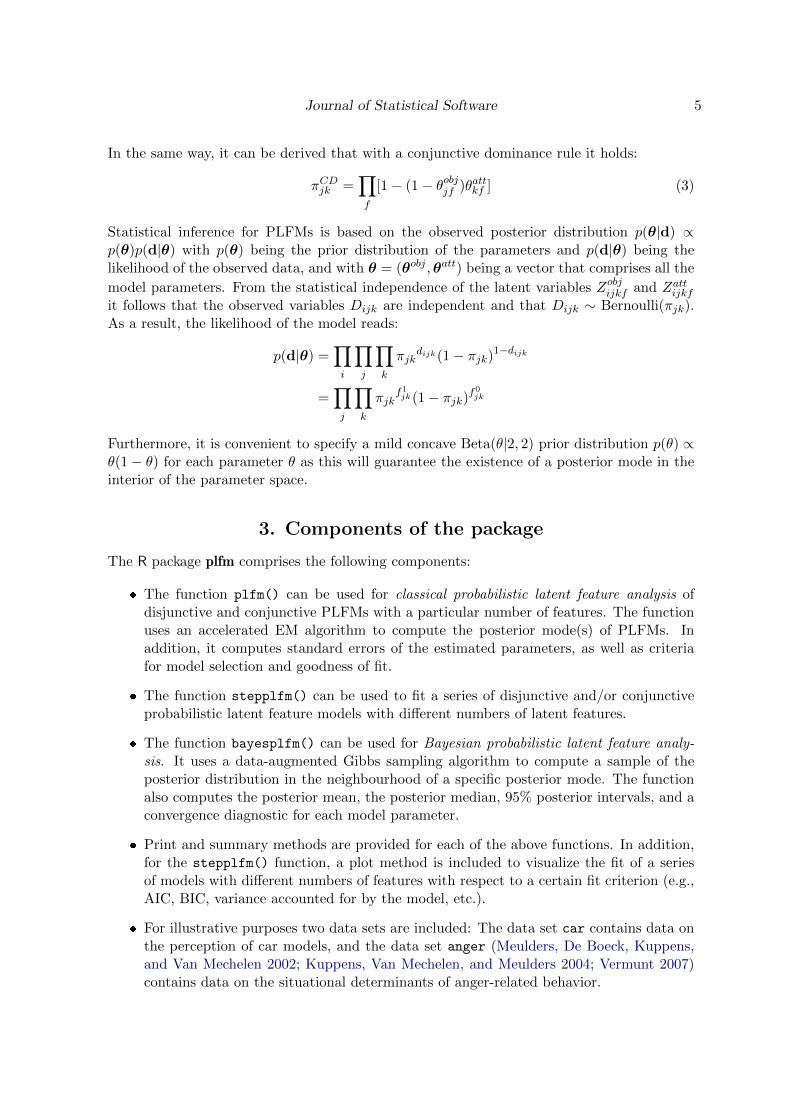
In order to choose the number of features, one may use the plot method of the stepplfm()
function to plot the BIC values of models with 1 up to 7 features:
R> plot(car.lst, which = "BIC")
As can be seen in Figure 1, a model with 6 features has the lowest BIC value, and hence itachieves the best balance between complexity and fit.
When using stepplfm() to compute a series of disjunctive (maprule = "disj") or conjunc-tive (maprule = "conj") models with minF up to maxF features, the results of subsequentplfm analyses are stored in a list with maxF-minF+1 components, each of which is a list ofclass "plfm". Using names(), a list of all attached entries can be obtained. For instance, forthe 6-feature model:
R> names(car.lst[[6]])
[1] "call" "objpar" "attpar" "fitmeasures"
[5] "logpost.runs" "objpar.runs" "attpar.runs" "bestsolution"
[9] "gradient.objpar" "gradient.attpar" "SE.objpar" "SE.attpar"
[13] "prob1"
with
� call: The parameters used to call the function.
� objpar: A J × F matrix of estimated object parameters for the best model (i.e., themodel with the highest posterior density among M runs).
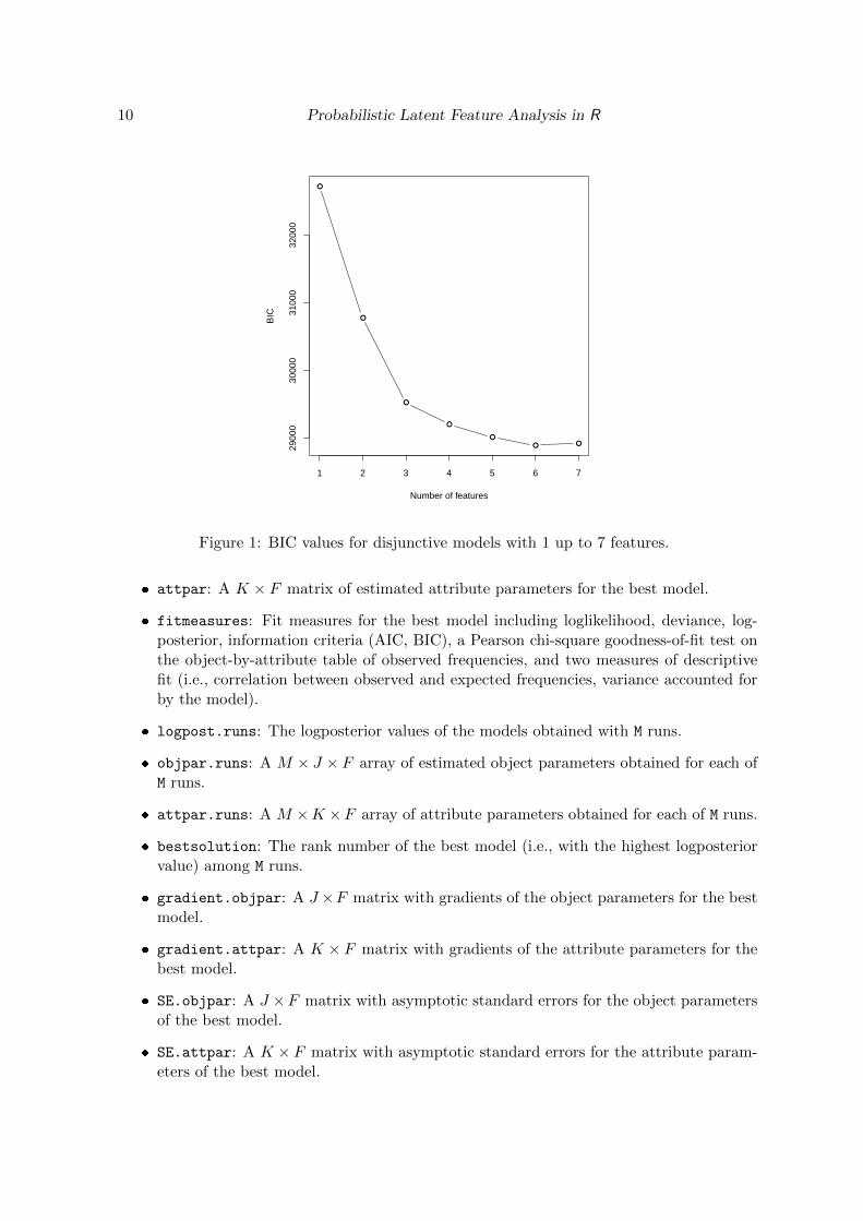
10 Probabilistic Latent Feature Analysis in R
●
●
●
●
●
● ●
1 2 3 4 5 6 7
2900
030
000
3100
032
000
Number of features
BIC
Figure 1: BIC values for disjunctive models with 1 up to 7 features.
� attpar: A K × F matrix of estimated attribute parameters for the best model.
� fitmeasures: Fit measures for the best model including loglikelihood, deviance, log-posterior, information criteria (AIC, BIC), a Pearson chi-square goodness-of-fit test onthe object-by-attribute table of observed frequencies, and two measures of descriptivefit (i.e., correlation between observed and expected frequencies, variance accounted forby the model).
� logpost.runs: The logposterior values of the models obtained with M runs.
� objpar.runs: A M × J × F array of estimated object parameters obtained for each ofM runs.
� attpar.runs: A M ×K ×F array of attribute parameters obtained for each of M runs.
� bestsolution: The rank number of the best model (i.e., with the highest logposteriorvalue) among M runs.
� gradient.objpar: A J×F matrix with gradients of the object parameters for the bestmodel.
� gradient.attpar: A K × F matrix with gradients of the attribute parameters for thebest model.
� SE.objpar: A J ×F matrix with asymptotic standard errors for the object parametersof the best model.
� SE.attpar: A K × F matrix with asymptotic standard errors for the attribute param-eters of the best model.

Journal of Statistical Software 11
● ● ● ● ● ● ● ● ● ● ● ●
●
●
●
● ● ● ● ●
5 10 15 20
−14
600
−14
590
−14
580
−14
570
run
logp
oste
rior
valu
e
Figure 2: Logarithm of the posterior density for disjunctive 6-feature models computed in M
= 20 runs.
� prob1: A J × K matrix of predicted object-attribute association probabilities for thebest model.
Using
R> plot(car.lst[[6]]$logpost.runs, xlab = "run", ylab = "logposterior value")
one may see in Figure 2 that 2 different solutions were identified with M = 20 runs, and thatthe best solution was obtained in 18 out of 20 runs.
To further inspect the fit and the estimated parameters for the best 6-feature model one mayprint the model output.
R> print(car.lst[[6]])
Call:
stepplfm(freq1 = car$freq1, freqtot = 78, maprule = "disj",
M = 20, F = 6)
DESCRIPTIVE FIT OBJECT X ATTRIBUTE TABLE:
Correlation observed and expected frequencies 0.960
VAF observed frequencies 0.922
ESTIMATE OBJECT PARAMETERS:

12 Probabilistic Latent Feature Analysis in R
F1 F2 F3 F4 F5 F6
Volkswagen Golf .67 .04 .12 .42 .02 .04
Opel Corsa .72 .01 .05 .01 .02 .03
Nissan Qashgai .04 .37 .60 .05 .04 .03
Toyota Prius .04 .03 .06 .03 .79 .05
BMW X5 .01 .64 .41 .56 .01 .01
Volvo V50 .06 .02 .77 .33 .14 .01
Renault Espace .03 .02 .95 .02 .04 .06
Citroen C4 Picasso .14 .01 .86 .01 .04 .05
Ford Focus Cmax .26 .03 .71 .02 .01 .03
Mercedes C-class .02 .15 .05 .89 .02 .07
Fiat 500 .28 .01 .01 .01 .04 .73
Audi A4 .15 .29 .28 .78 .04 .07
Mini Cooper .02 .43 .01 .18 .01 .78
Mazda MX5 .02 .84 .01 .02 .01 .11
ESTIMATE ATTRIBUTE PARAMETERS:
F1 F2 F3 F4 F5 F6
Economical .74 .01 .11 .01 .66 .24
Agile .65 .19 .06 .16 .09 .85
Environmentally friendly .31 .02 .04 .03 .81 .24
Reliable .54 .21 .25 .77 .40 .07
Practical .75 .03 .62 .15 .18 .41
Family Oriented .06 .02 .98 .14 .58 .01
Versatile .13 .08 .54 .22 .30 .04
Good price-quality ratio .67 .09 .24 .03 .31 .06
Luxurious .01 .46 .09 .87 .14 .09
Safe .29 .06 .33 .72 .28 .04
Sporty .15 .93 .01 .38 .08 .14
Attractive .17 .51 .10 .54 .10 .67
Comfortable .12 .15 .59 .72 .32 .05
Powerful .01 .58 .11 .63 .11 .02
Status symbol .03 .55 .02 .68 .20 .26
Technically advanced .01 .25 .02 .47 .69 .02
Sustainable .33 .08 .21 .52 .46 .05
Original .03 .20 .03 .02 .26 .63
Nice design .14 .47 .13 .33 .09 .60
Value for the money .43 .09 .15 .07 .15 .03
High trade-in value .06 .05 .01 .69 .05 .05
Exclusive .02 .24 .01 .09 .10 .28
Popular .71 .04 .22 .17 .09 .42
Outdoor .04 .36 .27 .03 .05 .01
Green .09 .01 .02 .02 .54 .10
City focus .69 .02 .01 .01 .32 .84
Workmanship .03 .18 .03 .45 .29 .03

Journal of Statistical Software 13
The printed output shows that the 6-feature disjunctive model fits the car-by-attribute fre-quencies very well: the model explains 92% of the variance in the observed frequencies.Furthermore, the estimated feature probabilities indicate that the extracted features have ameaningful interpretation. Feature 1 (F1) is likely to be ascribed to the small popular carmodels ‘Opel Corsa’ (0.72) and ‘Volkswagen Golf’ (0.67); and it has strong links with theattributes ‘practical’ (0.75), ‘economical’ (0.74), ‘popular’ (0.71), ‘city focus’ (0.69), ‘goodprice-quality ratio’ (0.67), ‘agile’ (0.65) and ‘reliable’ (0.54). Feature 2 (F2) has a very highprobability to be linked with the attribute ‘sporty’ (0.93), and has rather high probabilities tobe linked with powerful (0.58), ‘status symbol’ (0.55), ‘attractive’ (0.51), ‘nice design’ (0.47),and ‘luxurious’ (0.46). The feature is most likely to be perceived in the sports car ‘MazdaMX5’ (0.84) and also in the SUV ‘BMW X5’. Feature 3 (F3) is most likely to be ascribed tospatious family cars such as ‘Renault Espace’ (0.95), ‘Citroen C4 Picasso’ (0.86), ‘Volvo V50’(0.77), ‘Ford Focus Cmax’ (0.71), ‘Nissan Qashgai’ (0.60) and this feature has strong linkswith the attributes ‘family Oriented’ (0.98), ‘practical’ (0.62), ‘comfortable’ (0.59), ‘versatile’(0.54). Feature 4 (F4) has a high probability to be linked with the attributes ‘luxurious’(0.87), ‘reliable’ (0.77), ‘comfortable’ (0.72), ‘safe’ (0.72), ‘high trade-in value’(0.69), ‘statussymbol’ (0.68), ‘powerful’ (0.63) and ‘attractive’ (0.54). The feature is likely to be ascribed tothe rather expensive German car models ‘Mercedes C-class’ (0.89), ‘Audi A4’ (0.78), ‘BMWX5’ (0.56). Feature 5 (F5) is most likely perceived in the ‘Toyota Prius’ which uses hybriddrive technology to reduce CO2 emissions and to minimize gas consumption. The featurehas strong links with the attributes ‘environmentally friendly’ (0.81), ‘technically advanced’(0.69), ‘economical’ (0.66), ‘family oriented’ (0.58) and ‘green’ (0.54). Feature 6 (F6) is likelyto be linked with the attributes ‘agile’ (0.85), ‘city focus’ (0.84), ‘attractive’ (0.67), ‘original’(0.63), and ‘nice design’ (0.60). The feature is likely to be perceived in the small ‘Mini Cooper’(0.78), which has an original design and in the small ‘Fiat 500’ (0.73).
A more detailed summary of the model output including a Pearson chi-square goodness-of-fit test of the model on the car-by-attributes table, and asymptotic standard errors of theestimated object- and attribute parameters can be obtained using the summary function. Inparticular using
R> summary(car.lst[[6]])
we may see that that the model fails to fit the car-by-attribute frequencies in an absolute sense(χ2 = 571, df = 132, p < 0.01), and that the asymptotic standard errors of the estimatedparameters are acceptably low (i.e., always lower than .054 for object parameters and alwayslower than .074 for attribute parameters):
...
PEARSON CHI-SQUARE TEST OBJECT X ATTRIBUTE TABLE:
Pearson Chi-square 570.581
df 132.000
p-value 0.000
...

14 Probabilistic Latent Feature Analysis in R
STANDARD ERROR OBJECT PARAMETERS:
SE(F1) SE(F2) SE(F3) SE(F4) SE(F5) SE(F6)
Volkswagen Golf .032 .028 .039 .028 .018 .028
Opel Corsa .029 .009 .023 .006 .013 .020
Nissan Qashgai .021 .033 .035 .022 .020 .018
Toyota Prius .025 .021 .035 .018 .030 .025
BMW X5 .006 .043 .042 .033 .008 .008
Volvo V50 .028 .016 .037 .028 .030 .009
Renault Espace .021 .016 .023 .012 .019 .021
Citroen C4 Picasso .028 .008 .035 .006 .018 .022
Ford Focus Cmax .030 .018 .036 .014 .012 .019
Mercedes C-class .014 .047 .029 .024 .017 .025
Fiat 500 .034 .008 .011 .005 .020 .034
Audi A4 .031 .053 .046 .029 .024 .033
Mini Cooper .015 .044 .010 .026 .008 .034
Mazda MX5 .016 .032 .010 .015 .010 .027
...
STANDARD ERROR ATTRIBUTE PARAMETERS:
SE(F1) SE(F2) SE(F3) SE(F4) SE(F5) SE(F6)
Economical .053 .009 .026 .010 .071 .055
Agile .056 .045 .025 .041 .049 .053
Environmentally friendly .046 .018 .019 .019 .064 .048
Reliable .062 .047 .035 .042 .072 .045
Practical .058 .027 .034 .043 .062 .058
Family Oriented .032 .014 .017 .039 .074 .013
Versatile .042 .034 .032 .042 .065 .027
Good price-quality ratio .053 .030 .030 .021 .065 .036
Luxurious .013 .054 .023 .040 .052 .039
Safe .053 .033 .033 .042 .065 .029
Sporty .041 .038 .008 .049 .041 .055
Attractive .050 .056 .026 .048 .049 .061
Comfortable .042 .044 .034 .046 .068 .034
Powerful .013 .052 .024 .046 .046 .015
Status symbol .022 .055 .012 .046 .056 .057
Technically advanced .012 .043 .013 .042 .070 .019
Sustainable .054 .033 .030 .044 .071 .036
Original .020 .038 .015 .017 .059 .054
Nice design .044 .054 .026 .047 .046 .060
Value for the money .049 .028 .025 .028 .050 .023
High trade-in value .029 .027 .006 .038 .029 .028
Exclusive .015 .039 .007 .028 .041 .047
Popular .056 .030 .030 .039 .047 .056
Outdoor .021 .044 .028 .022 .031 .012

Journal of Statistical Software 15
Green .028 .010 .012 .014 .067 .030
City focus .054 .020 .010 .013 .066 .052
Workmanship .021 .038 .014 .040 .060 .024
5. Bayesian probabilistic latent feature analysis
5.1. Computation of a sample of the posterior
When using PLFMs for data analysis, it may interesting to go beyond merely locating theposterior mode(s) of the model and to compute a sample of the observed posterior distribution(Meulders et al. 2001b, 2002; Meulders, De Boeck, and Van Mechelen 2003; Meulders et al.2005). In particular, computing a sample of the posterior distribution is advantageous as itcan be used to (1) compute 100 ∗ (1−α)% posterior intervals of the model parameters whichare also valid in small samples, (2) simulate the distribution of (any function of) the modelparameters, (3) simulate the posterior predictive distribution of statistics (i.e., functions ofthe data), or of discrepancy measures (i.e., functions of the data and of the parameters) toevaluate the fit of the model.
To compute a sample of the observed posterior distribution p(θ|d) a data-augmented Gibbssampling algorithm was implemented in the package plfm. Assuming initial values θ(0), initeration m+ 1, the algorithm consists of the following steps:
1. Draw zobj(m+1)
from p(Zobj |θ(m),d).
2. Draw zatt(m+1)
from p(Zatt|θ(m), zobj(m+1)
,d).
3. Draw θ(m+1) from p(θ|zobj(m+1), zatt
(m+1),d).
It can be shown that the subsequent draws θ(1),θ(2), . . . form a Markov chain which con-verges to the true posterior distribution (Gelfand and Smith 1990; Tanner and Wong 1987).Appendix B provides further computational details about the different steps involved in the al-gorithm. Note that the proposed algorithm differs from the algorithm described by (Meulderset al. 2001b) in that latent object- and attribute classifications are sampled subsequently, andnot jointly. To evaluate the convergence of simulated chains to the true posterior distribution,we will use the approach suggested by (Gelman and Rubin 1992).
5.2. The function bayesplfm()
The function bayesplfm() can be used to compute a sample of the posterior distributionof disjunctive or conjunctive probabilistic latent feature models with a particular number offeatures using the proposed data-augmented Gibbs sampling algorithm.
The bayesplfm() function uses the same arguments as plfm() for the specification of theinput data (i.e., datatype, freq1, freqtot, data, object, attribute and rating), themapping rule (maprule) and the number of features (F). In addition, it includes the followingarguments:
� Nchains: The number of Markov-chains that are simulated using a data-augmentedGibbs sampling algorithm.

16 Probabilistic Latent Feature Analysis in R
� Nburnin: The number of burn-in iterations.
� maxNiter: The maximum number of iterations that will be computed for each chain.
� Nstep: The convergence of the chains to the true posterior will be checked for eachparameter after c*Nstep iterations with c=1,2,... The convergence will only be checkedwhen Nchains>1.
� Rhatcrit: The estimation procedure will be stopped if the R convergence diagnosticproposed by Gelman and Rubin (1992) is smaller than Rhatcrit for each object- andattribute parameter. By default Rhatcrit = 1.2.
� start.bayes: This argument can be used to define the type of starting point for theBayesian analysis. If start.bayes = "best" a preliminary plfm analysis (which in-volves M = 20 runs using random starting points) is conducted and the best solution ofthis analysis is used as the starting point for the Bayesian analysis. If start.bayes =
"fitted.plfm", the starting point is read from the plfm object assigned to the argu-ment fitted.plfm. If start.bayes = "random", a random starting point is used forthe Bayesian analysis.
� fitted.plfm: The name of the (plfm) object that contains posterior mode estimatesfor the specified model. Note that, any list object with as components a J × F ma-trix of object parameters object$objpar and a K × F matrix of attribute parametersobject$attpar can be used as an argument of fitted.plfm, and not only objects ofclass "plfm".
When applying PLFMs an important challenge is to efficiently explore the posterior distri-bution. This is complicated by the fact that the posterior distribution of PLFMs with F > 1is always multimodal: Different local maxima may exist and, in addition, for each local max-imum the posterior distribution consists of F ! identical posterior modes because one mayswitch the labels of the latent features.
In principle, both plfm() and bayesplfm() can be used to locate the mode(s) of the posteriordistribution for a specific PLFM (i.e., with a specific number of features and a certain mappingrule). However, using multiple plfm() runs with random starting points for this purposeis more efficient than simulating multiple chains with bayesplfm() from random startingpoints: First, the time to estimate a model is considerably shorter with plfm() than withbayesplfm(). Second, with the EM algorithm implemented in plfm(), each single run isensured to converge to a local maximum, whereas with bayesplfm() convergence using R isonly ensured if the simulated chains all sample from the same posterior mode. This conditionis most likely to be fulfilled if the different chains are started from one of the posterior modesdetected by plfm() (so that they will start sampling from the same mode by definition), andif different posterior modes are well-separated (so that the chains keep being stuck in the samemode and do no start visiting distinct posterior modes). Note that the latter is especiallyproblematic if the model tends the be overparameterized.
In sum, when applying PLFMs in practice, we recommend the following two-step data-analyticstrategy: First, use multiple runs of plfm() with random starting points to locate the modesof the posterior distribution. Second, use bayesplfm() with the best posterior mode as astarting point to compute a (local) sample in the neighbourhood of the posterior mode. Using

Journal of Statistical Software 17
bayesplfm() on the final model is often interesting because it provides a more accurateview on parameter uncertainty (e.g., posterior intervals which are valid in small samples),because the sample of the posterior can be used summarize the distribution of any functionof the parameters of interest, and because one may use the sample for further model checking(Gelman, Van Mechelen, Verbeke, Heitjan, and Meulders 2005; Meulders et al. 2001b, 2005).
Finally, note that using the best posterior mode as a starting point in the Bayesian analysisis fundamentally different from actually including information about the starting point in theprior distribution (e.g., by using a prior distribution which is centered at the best posteriormode): When using bayesplfm() with the best posterior mode as a starting point, theprior distribution involved in this Bayesian analysis is the same as the prior used by plfm()
(namely, a Beta(2,2) prior for each model parameter). In other words, the main goal of theBayesian analysis is to compute a sample of the posterior distribution in the neighbourhood ofa specific mode. As a (less efficient) alternative, one could also use random starting points andselect the chains that converge to the mode of interest. On the other hand, when includinginformation about the best posterior mode in the prior distribution (e.g., by using a strongprior distribution centered at the best posterior mode), one changes the prior distribution,and consequently also the posterior distribution. If the involved prior distribution is less vaguethan the Beta(2,2) prior, a Bayesian analysis using this adapted posterior will yield smallerposterior intervals than an analysis with a Beta(2,2) prior.
5.3. Bayesian probabilistic feature analysis of anger-related behavior
The list anger contains data on the situational determinants of anger-related behaviors (Meul-ders et al. 2002; Kuppens et al. 2004; Vermunt 2007). The raw data anger$data consist of asituation × behavior × person array of binary judgments of 101 first year psychology studentswho indicated whether or not they would display each of 8 anger-related behaviors when beingangry at someone in each of 6 situations. The 8 behaviors consist of 4 pairs of reactions thatreflect a particular strategy to deal with situations in which one is angry at someone, namely,(1) fighting (fly off the handle, quarrel), (2) fleeing (leave, avoid), (3) emotional sharing (pourout one’s heart, tell one’s story), and (4) making up (make up, clear up the matter). The sixsituations are constructed from two factors with three levels: (1) the extent to which one likesthe instigator of anger (like, dislike, unfamiliar), and (2) the status of the instigator of anger(higher, lower, equal). Each situation is presented as one level of a factor, without specifyinga level for the other factor. The elements of the matrix anger$freq1 contain the number ofpersons who indicated that they would display a certain behavior in a certain situation, andthe elements of the matrix anger$freqtot contain the total number of persons who made ajudgment for each situation-behavior pair.
After loading the data, we first use the plfm() function to estimate disjunctive and conjunctivemodels with 1 up to 3 features. Note that models with more than 3 features are not consideredas they do not have a positive number of degrees of freedom.
R> data("anger")
R> set.seed(78665)
R> anger.lst <- stepplfm(freq1 = anger$freq1, freqtot = anger$freqtot,
+ maprule = "disj/conj", minF = 1, maxF = 3, M = 20, emcrit1 = 1e-2,
+ emcrit2 = 1e-10)

18 Probabilistic Latent Feature Analysis in R
●
●●
1 2 3
6000
6100
6200
6300
6400
Number of features
BIC
●
●
●
Disjunctive
Conjunctive
Figure 3: BIC values for disjunctive and conjunctive models with 1 up to 3 features.
Next, to choose between the estimated models, we plot for the disjunctive and conjunctivemodels, the BIC values versus the number of features.
R> plot(anger.lst, which = "BIC")
As can be seen in Figure 3, the disjunctive 2-feature model offers the best balance betweencomplexity and goodness of fit as it has the lowest BIC value. Further inspection of the outputshows that this model deviates significantly from a perfectly fitting model (χ2 = 78.3, df =20, p < 0.01), but that it has a good descriptive fit in that it explains 92% of the variance inthe observed situation-behavior frequencies. To further study the disjunctive 2-feature model,we use the bayesplfm() function to compute a sample of the observed posterior distribution.In doing so, the (best) posterior mode which was identified with the plfm() function is usedas the starting point:
R> set.seed(34769)
R> bayesangerdisj2 <- bayesplfm(maprule = "disj", freq1 = anger$freq1,
+ freqtot = anger$freqtot, F = 2, maxNiter = 20000, Nburnin = 0,
+ Nstep = 5000, Nchains = 4, start.bayes = "fitted.plfm",
+ fitted.plfm = anger.lst$disj[[2]])
The algorithm stopped after 2000 iterations as for each parameter, the convergence diag-nostic R was smaller than the specified convergence criterion. The output generated by thebayesplfm() function is stored in a list of class "bayesplfm". Using names(), a list of allattached entries can be obtained. For instance, for the disjunctive 2-feature model:
R> names(bayesangerdisj2)

Journal of Statistical Software 19
[1] "call" "sample.objpar" "sample.attpar" "pmean.objpar"
[5] "pmean.attpar" "p95.objpar" "p95.attpar" "Rhat.objpar"
[9] "Rhat.attpar" "fitmeasures" "convstat"
with
� call: The parameters used to call the function.
� sample.objpar: A J×F ×Niter× Nchains array with parameter values for the objectparameters. The matrix sample.objpar[, , i, c] contains the draw of object parametersin iteration i of chain c. Note: when Nchains = 1 the chain length (Niter) equalsmaxNiter, and when Nchains > 1 the chain length equals the number of iterationsrequired to obtain convergence.
� sample.attpar: A K × F × Niter× Nchains array with parameter values for theattribute parameters.
� pmean.objpar: A J × F matrix with the posterior means of the object parameters.
� pmean.attpar: A K × F matrix with the posterior means of the attribute parameters.
� p95.objpar: A 3×J×F array which contains for each object parameter the percentiles2.5, 50 and 97.5.
� p95.attpar: A 3 ×K × F array which contains for each attribute parameter the per-centiles 2.5, 50 and 97.5.
� Rhat.objpar: A J × F matrix of R convergence values for the object parameters.
� Rhat.attpar: A K × F matrix of R convergence values for the attribute parameters
� fitmeasures: A list with two measures of descriptive fit on the J × K table: (1)the correlation between observed and expected frequencies, and (2) the proportion ofthe variance in the observed frequencies accounted for by the model. The associationprobabilities and corresponding expected frequencies are computed using the posteriormean of the parameters.
� convstat: The number of object- and attribute parameters that do not meet the con-vergence criterion.
To inspect the output of the model, one may print the object:
R> print(bayesangerdisj2)
CALL:
bayesplfm(freq1 = anger$freq1, freqtot = anger$freqtot, F = 2,
Nchains = 4, Nburnin = 0, maxNiter = 20000, Nstep = 5000,
maprule = "disj", start.bayes = "fitted.plfm",
fitted.plfm = anger.lst$disj[[2]])
NUMBER OF PARAMETERS THAT DO NOT MEET CONVERGENCE CRITERION:

20 Probabilistic Latent Feature Analysis in R
total number of parameters 28
number of parameters without convergence 0
DESCRIPTIVE FIT OBJECT X ATTRIBUTE TABLE:
Correlation observed and expected frequencies 0.959
VAF observed frequencies 0.920
POSTERIOR MEAN OBJECTPARAMETERS:
F1 F2
like .90 .43
dislike .16 .76
unfamiliar .06 .61
higher status .10 .85
lower status .79 .21
equal status .50 .69
POSTERIOR MEAN ATTRIBUTEPARAMETERS:
F1 F2
fly off the handle .55 .27
quarrel .58 .19
leave .09 .53
avoid .10 .64
pour out one's hart .28 .83
tell one's story .32 .92
make up .91 .10
clear up the matter .83 .11
Inspection of the estimated parameters shows that the extracted features have a meaningfulinterpretation. More specifically, the two features can be interpreted as situation-behaviorcomponents which are combined in a disjunctive manner.
The first component (F1) indicates that when being angry at a person one likes (0.90), orwhen being angry at a person of lower status (0.79), one is more likely to make up (makeup (0.91), clear up the matter (0.83)) or to fight (fly off the handle (0.55), quarrel (0.58)).The second component F2 indicates that when being angry at a person of higher status(0.85), or at a person one dislikes (0.76) or with whom one is unfamiliar (0.61), one is morelikely to react with emotional sharing (pour out one’s hart (0.83), tell one’s story (0.92)) orflighting (leave (0.53), avoid (0.64)) than with making up (make up (0.10), clear up the matter(0.11)) or fighting (fly off the handle (0.27), quarrel (0.19)). Finally, when being angry ata person of equal status both components are likely to play a role (i.e., for equal status theestimated feature probabilities for F1 and F2 equal 0.50 and 0.69, respectively), and they willbe combined in a disjunctive way.
In addition to the print function one may use the summary.bayesplfm() function to print a

Journal of Statistical Software 21
more detailed model output of the Bayesian analysis, which also shows 95% posterior intervalsand R convergence values for each of the parameters. In particular
R> summary(bayesangerdisj2)
...
95% POSTERIOR INTERVAL OBJECTPARAMETERS:
F1 F2
like [.793;.996] [.258;.595]
dislike [.054;.263] [.659;.887]
unfamiliar [.002;.136] [.52;.722]
higher status [.008;.2] [.741;.98]
lower status [.687;.921] [.032;.358]
equal status [.402;.616] [.573;.818]
RHAT CONVERGENCE OBJECTPARAMETERS:
F1 F2
like 1.168 1.084
dislike 1.106 1.037
unfamiliar 1.083 1.047
higher status 1.156 1.061
lower status 1.150 1.115
equal status 1.079 1.027
...
95% POSTERIOR INTERVAL ATTRIBUTEPARAMETERS:
F1 F2
fly off the handle [.441;.665] [.184;.364]
quarrel [.47;.699] [.094;.281]
leave [.003;.216] [.436;.629]
avoid [.004;.242] [.536;.754]
pour out one's hart [.062;.469] [.706;.963]
tell one's story [.122;.532] [.794;.996]
make up [.795;.994] [.008;.22]
clear up the matter [.712;.952] [.01;.22]
RHAT CONVERGENCE ATTRIBUTEPARAMETERS:
F1 F2
fly off the handle 1.044 1.067
quarrel 1.021 1.075
leave 1.057 1.021
avoid 1.014 1.028
pour out one's hart 1.076 1.041
tell one's story 1.093 1.081
make up 1.066 1.086
clear up the matter 1.074 1.097
22 Probabilistic Latent Feature Analysis in R
situation
prob
abili
ty
.0.2
.4.6
.81.
0
●
●
●
●
●
●
●
●
●
●
●
●
like
dislike
unfamiliar
higher status
lower status
equal status
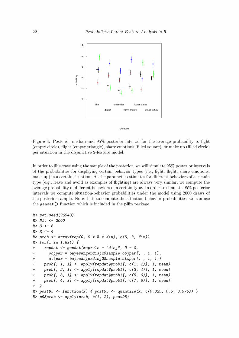
Figure 4: Posterior median and 95% posterior interval for the average probability to fight(empty circle), flight (empty triangle), share emotions (filled square), or make up (filled circle)per situation in the disjunctive 2-feature model.
In order to illustrate using the sample of the posterior, we will simulate 95% posterior intervalsof the probabilities for displaying certain behavior types (i.e., fight, flight, share emotions,make up) in a certain situation. As the parameter estimates for different behaviors of a certaintype (e.g., leave and avoid as examples of flighting) are always very similar, we compute theaverage probability of different behaviors of a certain type. In order to simulate 95% posteriorintervals we compute situation-behavior probabilities under the model using 2000 draws ofthe posterior sample. Note that, to compute the situation-behavior probabilities, we can usethe gendat() function which is included in the plfm package.
R> set.seed(96543)
R> Nit <- 2000
R> S <- 6
R> R <- 4
R> prob <- array(rep(0, S * R * Nit), c(S, R, Nit))
R> for(i in 1:Nit) {
+ repdat <- gendat(maprule = "disj", N = 0,
+ objpar = bayesangerdisj2$sample.objpar[, , i, 1],
+ attpar = bayesangerdisj2$sample.attpar[, , i, 1])
+ prob[, 1, i] <- apply(repdat$prob1[, c(1, 2)], 1, mean)
+ prob[, 2, i] <- apply(repdat$prob1[, c(3, 4)], 1, mean)
+ prob[, 3, i] <- apply(repdat$prob1[, c(5, 6)], 1, mean)
+ prob[, 4, i] <- apply(repdat$prob1[, c(7, 8)], 1, mean)
+ }
R> post95 <- function(x) { post95 <- quantile(x, c(0.025, 0.5, 0.975)) }
R> p95prob <- apply(prob, c(1, 2), post95)

Journal of Statistical Software 23
As can be seen in Figure 4, the visualization of the 95% posterior intervals is very usefulfor evaluating which type of behavior is most likely in a certain situation, and to evaluatewhether different behaviors have significantly different probabilities (i.e., non-overlapping 95%posterior intervals) to be displayed in a certain situation. For instance, Figure 4 shows thatwhen being angry at a person of equal status, it is significantly more likely to ‘share emotionswith someone’ than to ‘fight’, ‘flight’ or to ‘make up’. On the other hand, the probabilitiesfor ‘fighting’, ‘flighting’ or ‘making up’ in this situation do no significantly differ as their 95%posterior intervals overlap.
References
Agresti A (2002). Categorical Data Analysis. 2nd edition. John Wiley & Sons.
Akaike H (1973). “Information Theory and an Extension of the Maximum Likelihood Prin-ciple.” In BN Petrov, F Csaki (eds.), Second International Symposium on InformationTheory, pp. 271–283. Academiai Kiado, Budapest.
Akaike H (1974). “A New Look at the Statistical Model Identification.” IEEE Transactionson Automatic Control, 19, 716–723.
Candel MJJM, Maris E (1997). “Perceptual Analysis of Two-Way Two-Mode FrequencyData: Probability Matrix Decomposition and Two Alternatives.” International Journal ofResearch in Marketing, 14, 321–339.
Chessel D, Dufour AB, Thioulouse J (2004). “The ade4 Package I: One-Table Methods.” RNews, 4, 5–10. URL http://CRAN.R-project.org/doc/Rnews/.
Deerwester S, Dumais S, Furnas G, Landauer T, Harshman R (1990). “Indexing by LatentSemantic Analysis.” Journal of the American Society for Information Science, 41, 391–407.
Dray S, Dufour AB (2007). “The ade4 Package: Implementing the Duality Diagram forEcologists.” Journal of Statistical Software, 22(4), 1–20. URL http://www.jstatsoft.
org/v22/i04/.
Gelfand AE, Smith AFM (1990). “Sampling Based Approaches to Calculating MarginalDensities.” Journal of the American Statistical Association, 85, 398–409.
Gelman A, Rubin DB (1992). “Inference from Iterative Simulation Using Multiple Sequences.”Statistical Science, 7, 457–472.
Gelman A, Van Mechelen I, Verbeke G, Heitjan DF, Meulders M (2005). “Multiple Imputationfor Model Checking: Completed-Data Plots with Missing and Latent Data.” Biometrics,61, 74–85.
Hoffman DL, Franke GR (1986). “Correspondence Analysis: Graphical Representation ofCategorical Data in Marketing Research.” Journal of Marketing Research, 23, 213–217.
Husson F, Josse J, Le S, Mazet J (2012). FactoMineR: Multivariate Exploratory DataAnalysis and Data Mining with R. R package version 1.20, URL http://CRAN.R-project.
org/package=FactoMineR.
24 Probabilistic Latent Feature Analysis in R
Kuppens P, Van Mechelen I, Meulders M (2004). “Every Cloud Has a Silver Lining: Interper-sonal and Individual Differences Determinants of Anger-Related Behaviors.” Personalityand Social Psychology Bulletin, 30, 1550–1564.
Landauer T, Foltz P, Laham D (1998). “Introduction to Latent Semantic Analysis.” DiscourseProcesses, 25, 259–284.
Le S, Josse J, Husson F (2008). “FactoMineR: An R Package for Multivariate Analysis.”Journal of Statistical Software, 25(1), 1–18. URL http://www.jstatsoft.org/v25/i01/.
Louis TA (1982). “Finding Observed Information Using the EM Algorithm.” Journal of theRoyal Statistical Society B, 44, 98–130.
Maechler M, et al. (2013). sfsmisc: Utilities from Seminar fur Statistik ETH Zurich. R pack-age version 1.0-24, URL http://CRAN.R-project.org/package=sfsmisc.
Maris E, De Boeck P, Van Mechelen I (1996). “Probability Matrix Decomposition Models.”Psychometrika, 61, 7–29.
Meeds E, Ghahramani Z, Neal R, Roweis S (2007). “Modeling Dyadic Data with BinaryLatent Factors.” In B Scholkopf, J Platt, T Hoffman (eds.), Advances in Neural InformationProcessing Systems, volume 19. MIT Press, Cambridge.
Meulders M (2013). plfm: Probabilistic Latent Feature Analysis of Two-Way Two-ModeFrequency Data. R package version 1.1, URL http://CRAN.R-project.org/package=plfm.
Meulders M, De Boeck P, Kuppens P, Van Mechelen I (2002). “Constrained Latent ClassAnalysis of Three-Way Three-Mode Data.” Journal of Classification, 19, 277–302.
Meulders M, De Boeck P, Van Mechelen I (2001a). “Probability Matrix Decomposition Modelsand Main-Effects Generalized Linear Models for the Analysis of Replicated Binary Associ-ations.” Computational Statistics & Data Analysis, 38, 217–233.
Meulders M, De Boeck P, Van Mechelen I (2003). “A Taxonomy of Latent Structure Assump-tions for Probability Matrix Decomposition Models.” Psychometrika, 68, 61–77.
Meulders M, De Boeck P, Van Mechelen I, Gelman A (2005). “Probabilistic Feature Analysisof Facial Perception of Emotions.” Applied Statistics, 54, 781–793.
Meulders M, De Boeck P, Van Mechelen I, Gelman A, Maris E (2001b). “Bayesian Inferencewith Probability Matrix Decomposition Models.” Journal of Educational and BehavioralStatistics, 26, 153–179.
Miller K, Griffiths TL, Jordan MI (2009). “Nonparametric Latent Feature Models for LinkPrediction.” In Y Bengio, D Schuurmans, L J, CKI Williams (eds.), Advances in NeuralInformation Processing Systems, volume 22, pp. 1276–1284. MIT Press, Cambridge.
Nenadic O, Greenacre M (2007). “Correspondence Analysis in R, with Two- and Three-Dimensional Graphics: The ca Package.” Journal of Statistical Software, 20(3), 1–13. URLhttp://www.jstatsoft.org/v20/i03/.

Journal of Statistical Software 25
Oksanen J, Guillaume BF, Kindt R, Legendre P, Minchin PR, O’Hara RB, Simpson GL, Soly-mos P, Stevens MHH, Helene W (2012). vegan: Community Ecology Package. R packageversion 1.15-1, URL http://CRAN.R-project.org/package=vegan.
R Core Team (2013). R: A Language and Environment for Statistical Computing. R Founda-tion for Statistical Computing, Vienna, Austria. URL http://www.R-project.org/.
Schepers J, Hofmans J (2009). “TwoMP: A MATLAB Graphical User Interface for Two-ModePartitioning.” Behavior Research Methods, 41(2), 507–514.
Schepers J, Van Mechelen I, Ceulemans E (2011). “The Real-Valued Model of HierarchicalClasses.” Journal of Classification, 28, 363–389.
Schwarz G (1978). “Estimating the Dimensions of a Model.” The Annals of Statistics, 6,461–464.
Tanner MA (1996). Tools for Statistical Inference: Methods for the Exploration of PosteriorDistributions and Likelihood Functions. 3rd edition. Springer-Verlag.
Tanner MA, Wong WH (1987). “The Calculation of Posterior Distributions by Data Aug-mentation.” Journal of the American Statistical Association, 82, 528–540.
Torres A, Bijmolt THA (2009). “Assessing Brand Image Through Communalities and Asym-metries in Brand-to-Attribute and Attribute-to-Brand Associations.” European Journal ofOperational Research, 195, 628–640.
Tversky A (1977). “Features of Similarity.” Psychological Review, 84, 327–352.
Venables WN, Ripley BD (2002). Modern Applied Statistics with S. 4th edition. Springer-Verlag, New York.
Vermunt J (2007). “A Hierarchical Mixture Model for Clustering Three-Way Data Sets.”Computational Statistics & Data Analysis, 51, 5368–5376.
Wild F (2011). lsa: Latent Semantic Analysis. R package version 0.63-3, URL http://CRAN.
R-project.org/package=lsa.

26 Probabilistic Latent Feature Analysis in R
A. Optimization details
A.1. Expectation-maximization step
As with PLFMs the maximization step turns out to have a closed form solution (Maris et al.1996), closed form equations can be derived to update the parameter for each pair of EM-steps. In particular, using a disjunctive communality rule and a mild concave Beta(θ|2, 2)prior on each parameter θ, the following updating equations can be derived:
(θobjjf )(m)EM =
1 + Ez(∑
i
∑k Z
objijkf |d,θ
(m))
2 + IK(5)
=1 +
∑k[f1jkP (Zobj
ijkf = 1|Dijk = 1,θ(m)) + f0jkP (Zobjijkf = 1|Dijk = 0,θ(m))]
2 + IK(6)
and
(θattkf )(m)EM =
1 + Ez(∑
i
∑j Z
attijkf |d,θ
(m))
2 + IJ(7)
=1 +
∑j [f
1jkP (Zatt
ijkf = 1|Dijk = 1,θ(m)) + f0jkP (Zattijkf = 1|Dijk = 0,θ(m))]
2 + IJ(8)
Ignoring the iteration superscript, the conditional probabilities in Equation 6 and Equation 8can be computed as follows:
P (Zobjijkf = 1|Dijk = 1,θ) =
θobjjf θattkf + θobjjf (1− θattkf )[1−
∏q 6=f (1− θobjjq θ
attkq )]
1−∏
f (1− θobjjf θattkf )
P (Zobjijkf = 1|Dijk = 0,θ) =
θobjjf (1− θattkf )
1− θobjjf θattkf
P (Zattijkf = 1|Dijk = 1,θ) =
θobjjf θattkf + (1− θobjjf )θattkf [1−
∏q 6=f (1− θobjjq θ
attkq )]
1−∏
f (1− θobjjf θattkf )
P (Zattijkf = 1|Dijk = 0,θ) =
(1− θobjjf )θattkf
1− θobjjf θattkf
A.2. Newton-Raphson step
To implement the NR-step, we first note that it is straightforward to analytically derive thematrix of second derivatives in Equation 4. The results of these derivations are not listedhere. Second, the conditional expectation of the second derivative of the augmented posteriorwith respect to the object- or attribute parameters can be computed as follows:

Journal of Statistical Software 27
Ez
[−∂2log p(θ|d, z)
∂(θobjjf )2
∣∣∣∣∣d,θ(m)
]=
1 + Ez(∑
i
∑k Z
objijkf |d,θ
(m))
(θobjjf )2(9)
+1 + Ez(
∑i
∑k(1− Zobj
ijkf )|d,θ(m))
(1− θobjjf )2(10)
Ez
[−∂2log p(θ|d, z)
∂(θattkf )2
∣∣∣∣∣d,θ(m)
]=
1 + Ez(∑
i
∑j Z
attijkf |d,θ
(m))
(θattkf )2(11)
+1 + Ez(
∑i
∑j(1− Zatt
ijkf )|d,θm)
(1− θattkf )2(12)
The computation of the conditional expectations in (9), (10), (11), and (12) is similar as in(5) and (7).
A.3. First and second derivatives of log observed posterior
Assuming a disjunctive communality rule, the first derivative of the log observed posteriorwith respect to object- and attribute parameters can be computed as follows:
∂log p(θ|d)
∂θobjjf
=1
θobjjf
− 1
1− θobjjf
+∑k
[θattkf
1− θobjjf θattkf
][f1jk
(1− πjkπjk
)− f0jk
]and
∂log p(θ|d)
∂θattkf
=1
θattkf
− 1
1− θattkf
+∑j
[θobjjf
1− θobjjf θattkf
] [f1jk
(1− πjkπjk
)− f0jk
]In the same way, assuming a disjunctive communality rule, minus the second derivative of thelog observed posterior with respect to object- and attribute parameters reads as follows:
−∂2log p(θ|d)
∂(θobjjf )2=
1
(θobjjf )2+
1
(1− θobjjf )2+∑k
(θattkf
1− θobjjf θattkf
)2 [f1jk
(1− πjkπjk
)2
+ f0jk
]
and
−∂2log p(θ|d)
∂(θattkf )2=
1
(θattkf )2+
1
(1− θattkf )2+∑j
(θobjjf
1− θobjjf θattkf
)2 [f1jk
(1− πjkπjk
)2
+ f0jk
]
B. Computational details
For the disjunctive model, the steps of the data-augmented Gibbs sampling algorithm can beimplemented as follows:

28 Probabilistic Latent Feature Analysis in R
1. For each triple (i, j, k) draw zobjijk from
p(zobjijk |θ, dijk) ∝ p(dijk|zobjijk ,θatt)p(zobjijk |θ
obj)
with
p(dijk|zobjijk ,θatt) = [1−
∏f
(1− zobjijkfθattkf )]dijk [
∏f
(1− zobjijkfθattkf )]1−dijk
and
p(zobjijk |θobj) =
∏f
(θobjjf )zobjijkf (1− θobjjf )1−z
objijkf .
2. For each triple (i, j, k) draw zattijk from
p(zattijk|θatt, zobjijk , dijk) ∝ p(dijk|zobjijk , zattijk)p(zattijk|θatt)
with
p(dijk|zobjijk , zattijk) = [1−
∏f
(1− zobjijkfzattijkf )]dijk [
∏f
(1− zobjijkfzattijkf )]1−dijk
and
p(zattijk|θatt) =∏f
(θattkf )zattijkf (1− θattkf )1−z
attijkf .
3. For each pair (j, f) draw θobjjf from
Beta
(θobjjf |1 +
∑i
∑k
zobjijkf , 1 +∑i
∑k
(1− zobjijkf )
).
4. For each pair (k, f) draw θattkf from
Beta
θattkf |1 +∑i
∑j
zattijkf , 1 +∑i
∑j
(1− zattijkf )
.
Note that, to draw latent data vectors zobjijk or zattijk we use the function digitsBase() from theR package sfsmisc (Maechler et al. 2013) in order to compute a binary matrix which containsall latent data patterns.

Journal of Statistical Software 29
Affiliation:
Michel MeuldersFaculty of Economics and BusinessHUBrussel1000 Brussels, BelgiumE-mail: [email protected]: http://www.hubrussel.net/KBP/KBP-Homepage/KBP-medewerkersandDepartment of PsychologyKU LeuvenTiensestraat 102B-3000 Leuven, BelgiumURL: http://ppw.kuleuven.be/okp/home/
Journal of Statistical Software http://www.jstatsoft.org/
published by the American Statistical Association http://www.amstat.org/
Volume 54, Issue 14 Submitted: 2011-12-19August 2013 Accepted: 2013-03-29