Embed Size (px)
Citation preview
A numerical simulation of the
Jominy end{quench test
by D. H�omberg
Abstract
We present a numerical algorithm for simulating the Jominy end{quench test
and deriving continuous cooling diagrams. The underlying mathematical model for
the austenite{pearlite phase transition is based on Scheil's Additivity Rule and the
Johnson{Mehl equation. For the formation of martensite we compare the Koistinen{
Marburger formula with a rate law, which takes into account the irreversibility of
this process.
We carry out numerical simulations for the plain carbon steels C 1080 and C 100
W 1. The results suggest that the austenite{pearlite phase change may be described
decently by the Additivity Rule, except for the incubation time.
On the other hand, using a rate law to describe the martensite formation is
preferable to the Koistinen{Marburger formula, which leads to unphysical oscilla-
tions of the cooling curves in simulated CCT{diagrams.
1 Introduction
In this paper we describe a mathematical model for the phase transitions in eutectoid
carbon steel and use it to develop a numerical scheme for the simulation of the Jominy
end{quench test.
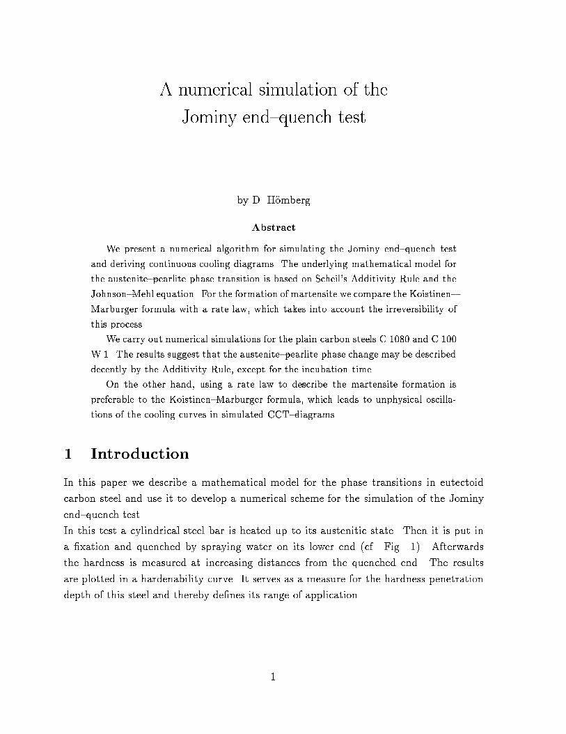
In this test a cylindrical steel bar is heated up to its austenitic state. Then it is put in
a �xation and quenched by spraying water on its lower end (cf. Fig. 1). Afterwards
the hardness is measured at increasing distances from the quenched end. The results
are plotted in a hardenability curve. It serves as a measure for the hardness penetration
depth of this steel and thereby de�nes its range of application.
1
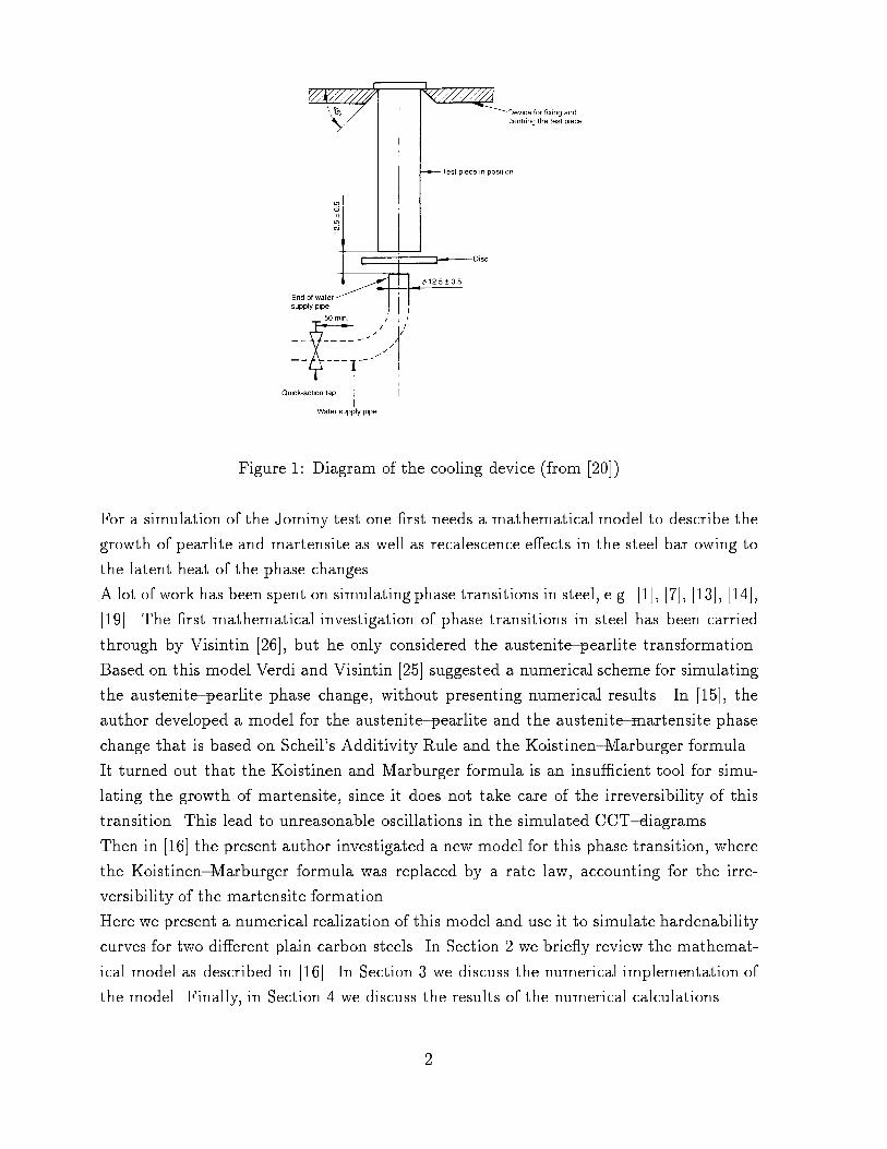
Figure 1: Diagram of the cooling device (from [20])
For a simulation of the Jominy test one �rst needs a mathematical model to describe the
growth of pearlite and martensite as well as recalescence e�ects in the steel bar owing to
the latent heat of the phase changes.
A lot of work has been spent on simulating phase transitions in steel, e.g. [1], [7], [13], [14],
[19]. The �rst mathematical investigation of phase transitions in steel has been carried
through by Visintin [26], but he only considered the austenite{pearlite transformation.
Based on this model Verdi and Visintin [25] suggested a numerical scheme for simulating
the austenite{pearlite phase change, without presenting numerical results. In [15], the
author developed a model for the austenite{pearlite and the austenite{martensite phase
change that is based on Scheil's Additivity Rule and the Koistinen{Marburger formula.
It turned out that the Koistinen and Marburger formula is an insu�cient tool for simu-
lating the growth of martensite, since it does not take care of the irreversibility of this
transition. This lead to unreasonable oscillations in the simulated CCT{diagrams.
Then in [16] the present author investigated a new model for this phase transition, where
the Koistinen{Marburger formula was replaced by a rate law, accounting for the irre-
versibility of the martensite formation.
Here we present a numerical realization of this model and use it to simulate hardenability
curves for two di�erent plain carbon steels. In Section 2 we brie y review the mathemat-
ical model as described in [16]. In Section 3 we discuss the numerical implementation of
the model. Finally, in Section 4 we discuss the results of the numerical calculations.
2
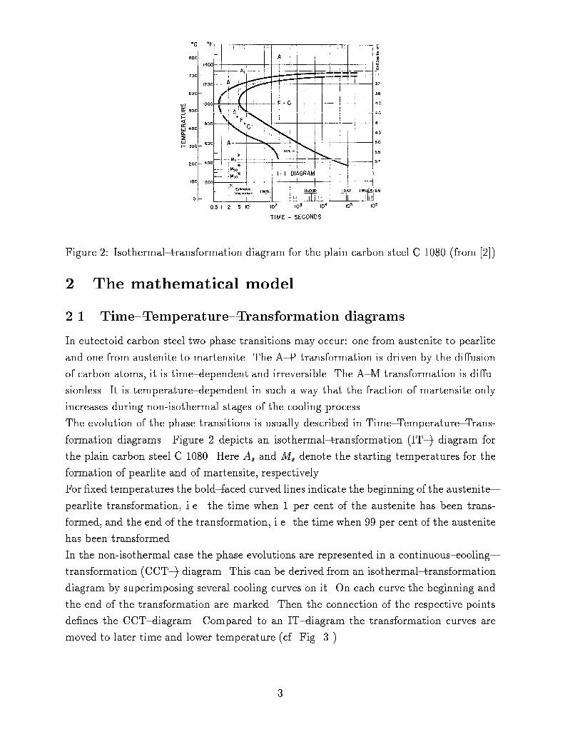
Figure 2: Isothermal{transformation diagram for the plain carbon steel C 1080 (from [2])
2 The mathematical model
2.1 Time{Temperature{Transformation diagrams
In eutectoid carbon steel two phase transitions may occur: one from austenite to pearlite
and one from austenite to martensite. The A{P transformation is driven by the di�usion
of carbon atoms, it is time{dependent and irreversible. The A{M transformation is di�u-
sionless. It is temperature{dependent in such a way that the fraction of martensite only
increases during non-isothermal stages of the cooling process.
The evolution of the phase transitions is usually described in Time{Temperature{Trans-
formation diagrams. Figure 2 depicts an isothermal{transformation (IT{) diagram for
the plain carbon steel C 1080. Here As and Ms denote the starting temperatures for the
formation of pearlite and of martensite, respectively.
For �xed temperatures the bold{faced curved lines indicate the beginning of the austenite{
pearlite transformation, i.e. the time when 1 per cent of the austenite has been trans-
formed, and the end of the transformation, i.e. the time when 99 per cent of the austenite
has been transformed.
In the non-isothermal case the phase evolutions are represented in a continuous{cooling{
transformation (CCT{) diagram. This can be derived from an isothermal{transformation
diagram by superimposing several cooling curves on it. On each curve the beginning and
the end of the transformation are marked. Then the connection of the respective points
de�nes the CCT{diagram. Compared to an IT{diagram the transformation curves are
moved to later time and lower temperature (cf. Fig. 3 ).
3
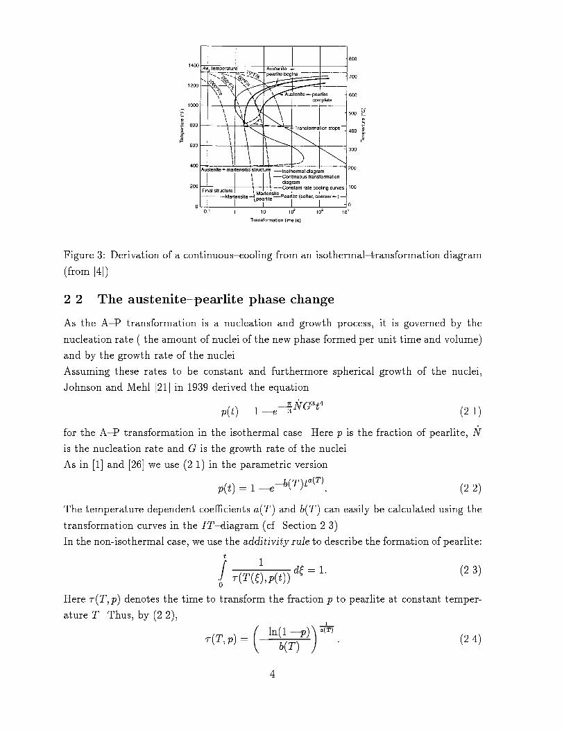
Figure 3: Derivation of a continuous{cooling from an isothermal{transformation diagram
(from [4])
2.2 The austenite{pearlite phase change
As the A{P transformation is a nucleation and growth process, it is governed by the
nucleation rate ( the amount of nuclei of the new phase formed per unit time and volume)
and by the growth rate of the nuclei.
Assuming these rates to be constant and furthermore spherical growth of the nuclei,
Johnson and Mehl [21] in 1939 derived the equation
p(t) = 1� e��
3_NG3t4 (2.1)
for the A{P transformation in the isothermal case. Here p is the fraction of pearlite, _N
is the nucleation rate and G is the growth rate of the nuclei.
As in [1] and [26] we use (2.1) in the parametric version
p(t) = 1� e�b(T )ta(T )
: (2.2)
The temperature dependent coe�cients a(T ) and b(T ) can easily be calculated using the
transformation curves in the IT{diagram (cf. Section 2.3).
In the non-isothermal case, we use the additivity rule to describe the formation of pearlite:
tZ0
1
� (T (�); p(t))d� = 1: (2.3)
Here � (T; p) denotes the time to transform the fraction p to pearlite at constant temper-
ature T . Thus, by (2.2),
� (T; p) =
�
ln(1� p)
b(T )
! 1a(T )
: (2.4)
4
Equation (2.4) was derived by Scheil [24] to predict the incubation period of the A{
P transformation. Later Avrami [5] and Cahn [8] showed that (3.4) can be applied to
characterize the kinetics of a class of phase changes which they called additive.
Although the pearlite phase change is not an additive transformation in their sense, (cf.
[9]), according to a comparative investigation by Hayes [12] the additivity rule is a better
tool for predicting the course of the phase change than a rate law. Moreover, meas-
urements by Hawbolt et al. [13] show that also in quantity the A{P transformation is
described well by the additivity rule, except for the incubation period where the pearlite
fraction predicted by the additivity rule shows only poor coincidence with the measure-
ments. It should be noticed that equations of this type are also used for modelling fatigue
e�ects, e.g. the Palmgren{Minor rule (cf. [6]).
A di�erent approach to model a nucleation and growth process was chosen by Andreucci
et al. [3]. Going back to the ideas of Johnson and Mehl they derived an integral equation
to describe the solidi�cation of polymers in the non-isothermal case.
2.3 Identifying coe�cients from IT{diagrams
Assuming that the generalized Johnson {Mehl{equation (2.2) appropriately describes the
isothermal evolution of the phase fractions we present a simple method to obtain the data
functions a(T ) and b(T ) from the IT{diagrams.
Since the bold{faced curves in these diagrams are the 'iso{fractions' p = 0:01 and p = 0:99,
we interpret these transformation curves as the respective graphs of functions
ts : [Ms; As] ! IR+; tf : [Ms; As] ! IR+;
which measure the beginning and end of the pearlitic transformation for given temper-
ature. These data functions can be drawn from the IT{diagram. Then the wanted
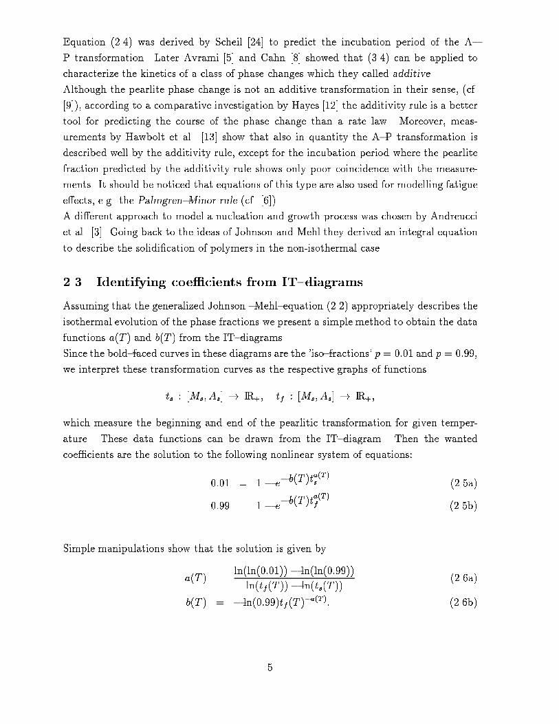
coe�cients are the solution to the following nonlinear system of equations:
0:01 = 1 � e�b(T )ta(T )s (2.5a)
0:99 = 1 � e�b(T )t
a(T )
f (2.5b)
Simple manipulations show that the solution is given by
a(T ) =ln(ln(0:01))� ln(ln(0:99))
ln(tf(T ))� ln(ts(T ))(2.6a)
b(T ) = � ln(0:99)tf (T )�a(T ): (2.6b)
5
0
0.5
1
1.5
2
2.5
3
3.5
4
0 100 200 300 400 500 600 700 800
a(T
)
T
0
0.005
0.01
0.015
0.02
0.025
0 100 200 300 400 500 600 700 800
b(T
)
T
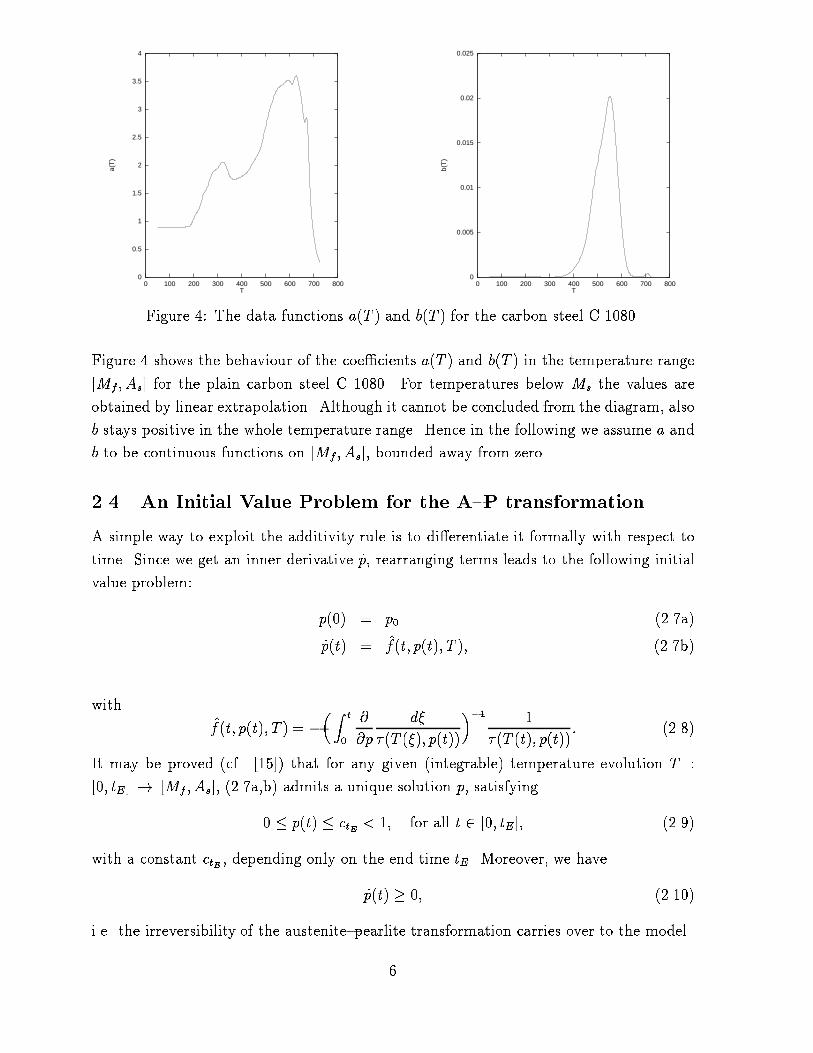
Figure 4: The data functions a(T ) and b(T ) for the carbon steel C 1080.
Figure 4 shows the behaviour of the coe�cients a(T ) and b(T ) in the temperature range
[Mf ; As] for the plain carbon steel C 1080. For temperatures below Ms the values are
obtained by linear extrapolation. Although it cannot be concluded from the diagram, also
b stays positive in the whole temperature range. Hence in the following we assume a and
b to be continuous functions on [Mf ; As], bounded away from zero.
2.4 An Initial Value Problem for the A{P transformation
A simple way to exploit the additivity rule is to di�erentiate it formally with respect to
time. Since we get an inner derivative _p, rearranging terms leads to the following initial
value problem:
p(0) = p0 (2.7a)
_p(t) = f(t; p(t); T ); (2.7b)
with
f (t; p(t); T ) = �
�Zt
0
@
@p
d�
� (T (�); p(t))
��1 1
� (T (t); p(t)): (2.8)
It may be proved (cf. [15]) that for any given (integrable) temperature evolution T :
[0; tE] ! [Mf ; As]; (2.7a,b) admits a unique solution p, satisfying
0 � p(t) � ctE< 1; for all t 2 [0; tE]; (2.9)
with a constant ctE, depending only on the end time tE. Moreover, we have
_p(t) � 0; (2.10)
i.e. the irreversibility of the austenite{pearlite transformation carries over to the model.
6
Unfortunately, as �gure 4 shows, the coe�cient a, which was equal to 4 in the original
Johnson{Mehl equation and assumed to be greater than 1 in [25] and [26], actually takes
values less then 1, if the temperature is in a range just below As. In this case, we can
prove the following
Proposition 2.1 Let T : [0; tE] ! [Mf ; As] be a continuous function, such that
a(T (t)) < 1 for all 0 � t � ~t;
then the following are valid:
limt!0(+)
p(t) = 0; (2.11a)
limt!0(+)
_p(t) = 1: (2.11b)
For the proof, we refer to [15].
In a nucleation and growth process the increase of the volume fraction of the new phase
should be 'small' during the incubation time, which is a contradiction to (2.11b). Thus,
Proposition 2.1 gives the mathematical reason, why the additivity rule does not work well
for the early stages of the transformation. As said before, this fact has also been observed
experimentally.
To overcome this di�culty, we adopt the following philosophy: We de�ne an incubation
time tI , which we keep �xed. Giving up the aim of predicting the exact evolution kinetics
during this incubation time, we just gauge the process by demanding that the additivity
rule shall hold, when the end of the incubation time is reached. This leads to the following
model:
� Let T : [0; tE]! IR be a given temperature evolution,
� tI 2 (0; tE) the �xed incubation time, then, depending on T ,
� p0 is de�ned by ZtI
0
1
� (T (�); p0)d� = 1: (2.12)
� The fraction of pearlite is determined by the following initial value problem (IVP):
p(0) = p0; (2.13a)
_p(t) =
8<: 0 ; 0 < t � tI
f(t; p(t); T )H(As � T (t)) ; tI < t < tE:(2.13b)
The heaviside function
H(x) =
8<: 1; x > 0
0; x � 0
prevents the formation of pearlite above the critical temperature As.
7
2.5 The austenite{martensite phase change
While the additivity rule is a well investigated decent tool for describing the growth of
pearlite, there seems to be no satisfactory model at hand for the martensitic transforma-
tion in steel.
Usually, exponential growth laws like the Koistinen and Marburger formula
m(t) = 1� e�c(Ms�T (t)) (2.14)
are used (cf. [15], [17], [18]).
These equations have all in common that they do not model the irreversibility of the
austenite { martensite phase transition. Thus, in numerical simulations based on these
models, owing to the release of latent heat, usually a decrease in the martensite fraction
is observed (cf. [15] and Section 4).
The formation of martensite starts below the critical temperature Ms, and the volume
fraction of martensite only grows during non-isothermal stages of a cooling process.
At this stage of the exposition, where we assume the temperature evolution to be known
a priori, one could argue that growth laws like (2.14) are still valid, if only they are
modi�ed by the logical statement that the volume fraction of martensite never decreases.
For instance, one could replace (2.14) with
m(t) = maxs2[0;t]
�1 � e�c(Ms�T (s))
�: (2.14')
But, owing to the latent heat, the phase transitions interact with the temperature
evolution. Therefore, it is important to keep track of the actual transformation kinetics.
Hence, we propose the following rate law for the growth of martensite:
m(0) = 0; (2.15a)
_m(t) = (1�m(t))G(T (t))H(�Tt(t)): (2.15b)
Here, again H is the heaviside function. G shall be bounded, positive and (Lipschitz{)
continuous, satisfying G(x) = 0 for all x �Ms. Putting m(0) = 0, we tacitly assume that
we start with a temperature T (0) > Ms.
If during some stage of a heat treatment cycle either T � Ms or T is increasing, i.e.
Tt � 0, according to (2.15b) we have _m(t) = 0, whence no martensite is produced during
this stage.
Moreover, since _m � 0, the irreversibility of the martensite transformation is now incor-
porated in the model.
8
2.6 The complete model
In (2.13b) and (2.15b), actually, not the fractions p and m occur but the volume fraction
of austenite which is 1� p or 1�m, respectively. Therefore, to combine both models one
only has to replace these terms by the volume fraction of austenite in the case when both
pearlite and martensite are present, i.e. 1� p �m.
So we end up with the following initial value problem for the phase transitions in eutectoid
carbon steel:
p(0) = p0; (2.16a)
m(0) = 0; (2.16b)
_p(t) = (1� p(t)�m(t))f(t; p(t);m(t); T )H(As � T (t)); (2.16c)
_m(t) = (1� p(t)�m(t))G(T (t))H(�Tt(t)); (2.16d)
where we de�ne
f(t; p;m; T )) := �
�Zt
0
d�
a(T (�))� (T (�); p;m)
��1 ln(1� p �m)
� (T (t); p;m))H(t� tI): (2.17)
Here, � (T; p;m) is de�ned by
� (T; p;m) =
��
ln(1 � p�m)
b(T )
� 1a(T ) : (2.18)
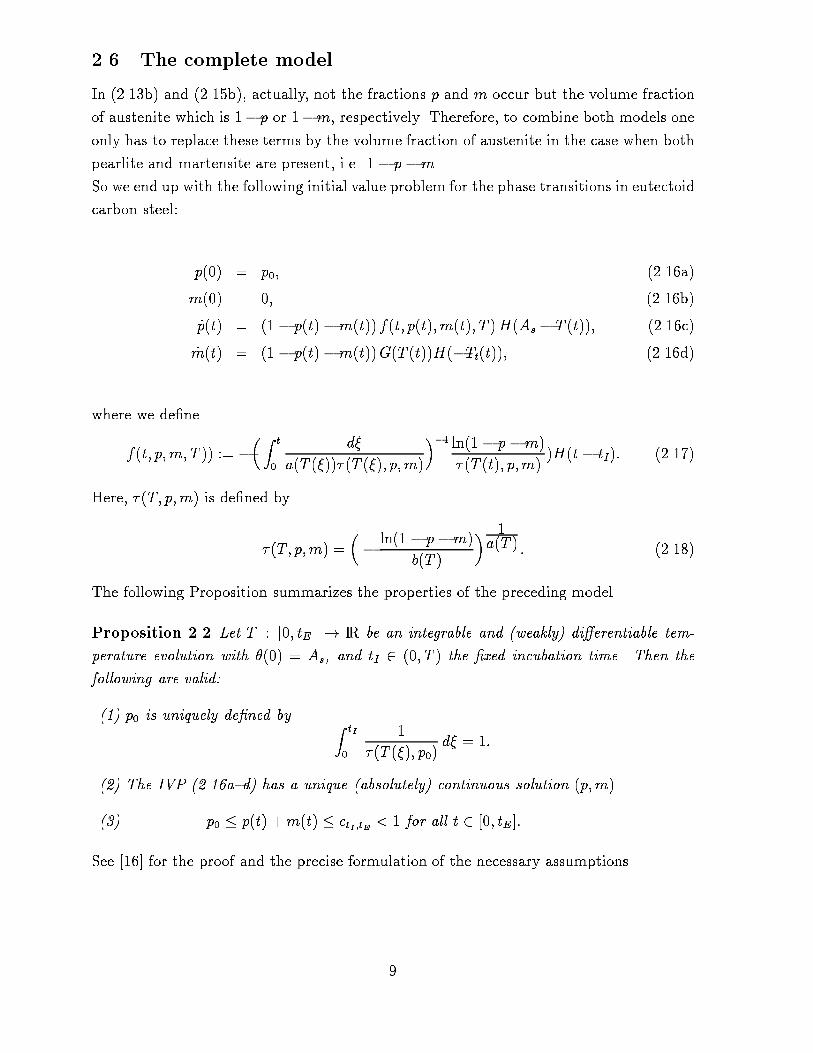
The following Proposition summarizes the properties of the preceding model.
Proposition 2.2 Let T : [0; tE] ! IR be an integrable and (weakly) di�erentiable tem-
perature evolution with �(0) = As, and tI 2 (0; T ) the �xed incubation time. Then the
following are valid:
(1) p0 is uniquely de�ned by ZtI
0
1
� (T (�); p0)d� = 1:
(2) The IVP (2.16a{d) has a unique (absolutely) continuous solution (p;m).
(3) p0 � p(t) +m(t) � ctI ;tE < 1 for all t 2 [0; tE]:
See [16] for the proof and the precise formulation of the necessary assumptions.
9
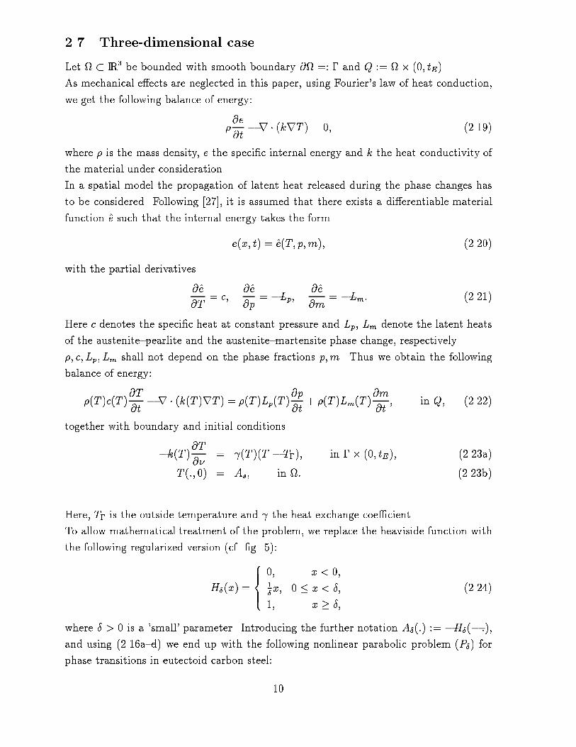
2.7 Three-dimensional case
Let � IR3 be bounded with smooth boundary @ =: � and Q := � (0; tE).
As mechanical e�ects are neglected in this paper, using Fourier's law of heat conduction,
we get the following balance of energy:
�@e
@t�r � (krT ) = 0; (2.19)
where � is the mass density, e the speci�c internal energy and k the heat conductivity of
the material under consideration.
In a spatial model the propagation of latent heat released during the phase changes has
to be considered. Following [27], it is assumed that there exists a di�erentiable material
function e such that the internal energy takes the form
e(x; t) = e(T; p;m); (2.20)
with the partial derivatives
@e
@T= c;
@e
@p= �Lp;
@e
@m= �Lm: (2.21)
Here c denotes the speci�c heat at constant pressure and Lp, Lm denote the latent heats
of the austenite{pearlite and the austenite{martensite phase change, respectively.
�; c; Lp; Lm shall not depend on the phase fractions p;m. Thus we obtain the following
balance of energy:
�(T )c(T )@T
@t�r � (k(T )rT ) = �(T )Lp(T )
@p
@t+ �(T )Lm(T )
@m
@t; in Q; (2.22)
together with boundary and initial conditions
�k(T )@T
@�= (T )(T � T�); in �� (0; tE); (2.23a)
T (:; 0) = As; in : (2.23b)
Here, T� is the outside temperature and the heat exchange coe�cient.
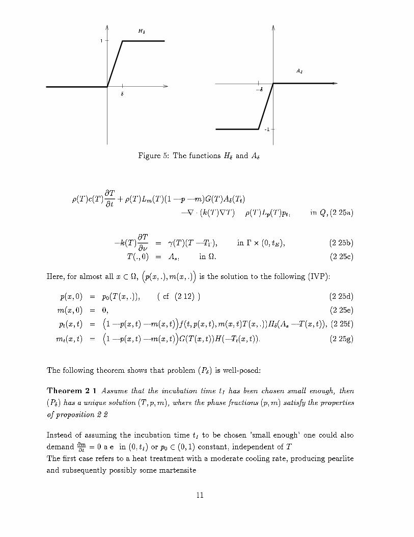
To allow mathematical treatment of the problem, we replace the heaviside function with
the following regularized version (cf. �g. 5):
H�(x) =
8>><>>:
0; x < 0;1�x; 0 � x < �;
1; x � �;
(2.24)
where � > 0 is a 'small' parameter. Introducing the further notation A�(:) := �H�(� :),
and using (2.16a{d) we end up with the following nonlinear parabolic problem (P�) for
phase transitions in eutectoid carbon steel:
10
�
H�
1
��
-1
A�
Figure 5: The functions H� and A�.
�(T )c(T )@T
@t+ �(T )Lm(T )(1� p�m)G(T )A�(Tt)
�r � (k(T )rT ) = �(T )Lp(T )pt; in Q; (2.25a)
�k(T )@T
@�= (T )(T � T�); in �� (0; tE); (2.25b)
T (:; 0) = As; in : (2.25c)
Here, for almost all x 2 ,�p(x; :);m(x; :)
�is the solution to the following (IVP):
p(x; 0) = p0(T (x; :)); ( cf. (2.12) ) (2.25d)
m(x; 0) = 0; (2.25e)
pt(x; t) =�1� p(x; t)�m(x; t)
�f(t; p(x; t);m(x; t)T (x; :))H�(As � T (x; t)); (2.25f)
mt(x; t) =�1� p(x; t)�m(x; t)
�G(T (x; t))H(�Tt(x; t)): (2.25g)
The following theorem shows that problem (P�) is well-posed:
Theorem 2.1 Assume that the incubation time tI has been chosen small enough, then
(P�) has a unique solution (T; p;m), where the phase fractions (p;m) satisfy the properties
of proposition 2.2.
Instead of assuming the incubation time tI to be chosen 'small enough' one could also
demand @m
@t= 0 a.e. in (0; tI) or p0 2 (0; 1) constant, independent of T .
The �rst case refers to a heat treatment with a moderate cooling rate, producing pearlite
and subsequently possibly some martensite.
11
The second condition applies to quench cooling, i.e. very fast cooling to achieve a nearly
pure martensitic structure. In this case it is reasonable to assume p0 to be constant,
because no more pearlite will be formed during the cooling process.
From a mathematical point of view it is interesting to see what happens if the regulariza-
tion parameter � tends to zero. This question has been investigated in [16], we only want
to remark here that one still gets a solution in this case. For the proof, we had to assume
that Lp; Lm are (Lipschitz) continuous, positive, bounded functions of temperature T ,
and that �; c; k; are positive constants.
If one is only interested in the case � > 0 �xed, which is clearly the most important case
in view of practical applications, Theorem 2.1 can be proved assuming that is continu-
ously di�erentiable and �; c; k are (Lipschitz) continuous, positive, bounded functions of
temperature T . Moreover, they may depend on x and t in a rather general way.
A dependency of � and c on the phase fractions is not covered by this theory and would
require further analysis. Probably it would be di�cult to prove uniqueness in this case.
What is more, it seems to be doubtful, whether one would be able to obtain enough
measurements to include this dependency in numerical simulations.
3 Numerical method
3.1 The algorithm
In this section we will apply our model to simulate the Jominy end{quench test. Owing
to the symmetries of the problem (cf. Fig. 1), we make use of cylindrical coordinates.
Thus, we obtain the following energy balance:
A(T )@T
@t�
@
@r
�k(T )
@T
@r
��
k(T )
r
@T
@r�
@
@z
�k(T )
@T
@z
�= B(T ); in � (0; T ); (3.1)
with = (0; R) � (0;H), where R is the radius and H the height of the steel bar.
Moreover we have used the abbreviations
A(T ) = �(T )c(T ) (3.2)
B(T ) = �(T )Lp(T )f1(p;m; T ) + �(T )Lm(T )f2(p;m; T ); (3.3)
where f1 anf f2 are the right{hand sides in (2.25f,g).
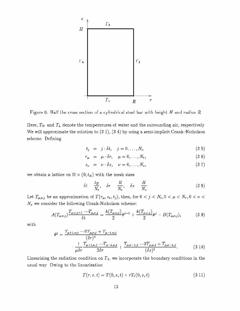
According to Figure 6, we consider the following boundary conditions:
�k(T )@T
@�=
8>>>>><>>>>>:
�(T � TW ); in �1 � (0; tE);
�(T 4� T 4
L); in �2 � (0; tE);
0; in �3 � (0; tE);
0; in �4 � (0; tE):
(3.4)
12
z
r
�4
�1
�2
R
H�3
Figure 6: Half the cross section of a cylindrical steel bar with height H and radius R.
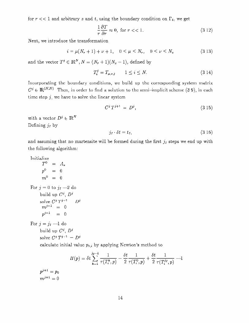
Here, TW and TL denote the temperatures of water and the surrounding air, respectively.
We will approximate the solution to (3.1), (3.4) by using a semi-implicit Crank{Nicholson
scheme. De�ning
tj = j � �t; j = 0; : : : ; Nt; (3.5)
r� = � � �r; � = 0; : : : ; Nr; (3.6)
z� = � � �z; � = 0; : : : ; Nz; (3.7)
we obtain a lattice on � (0; tE) with the mesh sizes
�t =tE
Nt
; �r =R
Nr
; �z =H
Nz
: (3.8)
Let T�;�;j be an approximation of T (r�; z�; tj), then, for 0 < j < Nt; 0 < � < Nr; 0 < � <
Nz we consider the following Crank-Nicholson scheme:
A(T�;�;j)T�;�;j+1 � T�;�;j
�t=k(T�;�;j)
2�j+1 +
k(T�;�;j)
2�j +B(T�;�;j); (3.9)
with
�j =T�+1;�;j � 2T�;�;j + T��1;�;j
(�r)2
+1
��r
T�+1;�;j � T��1;�;j
2�r+T�;�+1;j � 2T�;�;j + T�;��1;j
(�z)2: (3.10)
Linearizing the radiation condition on �2, we incorporate the boundary conditions in the
usual way. Owing to the linearization
T (r; z; t) = T (0; z; t) + rTr(0; z; t) (3.11)
13
for r << 1 and arbitrary z and t, using the boundary condition on �4, we get
1
r
@T
@r� 0; for r << 1: (3.12)
Next, we introduce the transformation
i = �(Nr + 1) + � + 1; 0 � � � Nr; 0 � � � Nz (3.13)
and the vector T j2 IRN ; N = (Nr + 1)(Nz + 1), de�ned by
T j
i= T�;�;j 1 � i � N: (3.14)
Incorporating the boundary conditions, we build up the corresponding system matrix
Cj2 IR(N;N). Then, in order to �nd a solution to the semi{implicit scheme (3.9), in each
time step j, we have to solve the linear system
Cj T j+1 = Dj ; (3.15)
with a vector Dj2 IRN .
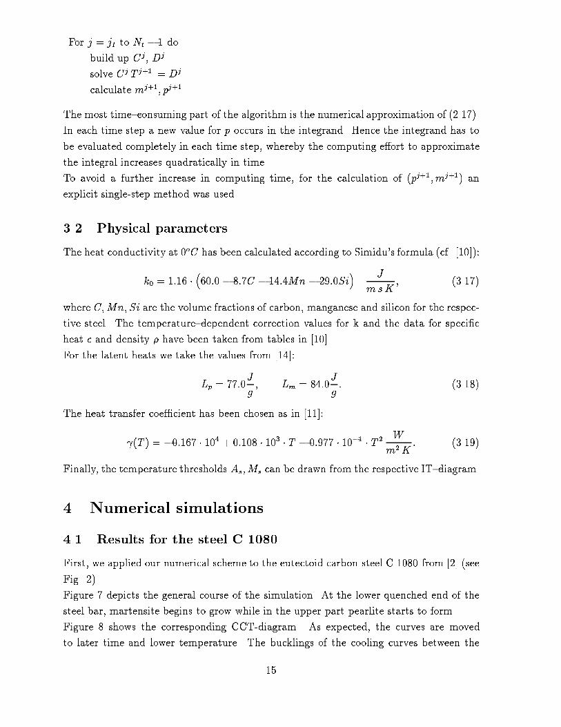
De�ning jI by
jI � �t = tI; (3.16)
and assuming that no martensite will be formed during the �rst jI steps we end up with
the following algorithm:
InitializeT 0 = As
p0 = 0
m0 = 0
For j = 0 to jI � 2 do
build up Cj, Dj
solve Cj T j+1 = Dj
mj+1 = 0
pj+1 = 0
For j = jI � 1 do
build up Cj, Dj
solve Cj T j+1 = Dj
calculate initial value p0;i by applying Newton's method to
H(p) = �tjI�1Xk=1
1
� (T k
i; p)
+�t
2
1
� (T 0i; p)
+�t
2
1
� (T jI
i; p)
� 1
pj+1 = p0
mj+1 = 0
14
For j = jI to Nt � 1 do
build up Cj, Dj
solve Cj T j+1 = Dj
calculate mj+1; pj+1.
The most time{consuming part of the algorithm is the numerical approximation of (2.17).
In each time step a new value for p occurs in the integrand. Hence the integrand has to
be evaluated completely in each time step, whereby the computing e�ort to approximate
the integral increases quadratically in time.
To avoid a further increase in computing time, for the calculation of (pj+1;mj+1) an
explicit single-step method was used.
3.2 Physical parameters
The heat conductivity at 0oC has been calculated according to Simidu's formula (cf. [10]):
k0 = 1:16 ��60:0 � 8:7C � 14:4Mn � 29:0Si
� J
msK; (3.17)
where C;Mn; Si are the volume fractions of carbon, manganese and silicon for the respec-
tive steel. The temperature{dependent correction values for k and the data for speci�c
heat c and density � have been taken from tables in [10].
For the latent heats we take the values from [14]:
Lp = 77:0J
g; Lm = 84:0
J
g: (3.18)
The heat transfer coe�cient has been chosen as in [11]:
(T ) = �0:167 � 104 + 0:108 � 103 � T � 0:977 � 10�1 � T 2 W
m2K: (3.19)
Finally, the temperature thresholds As;Ms can be drawn from the respective IT{diagram.
4 Numerical simulations
4.1 Results for the steel C 1080
First, we applied our numerical scheme to the eutectoid carbon steel C 1080 from [2] (see
Fig. 2).
Figure 7 depicts the general course of the simulation. At the lower quenched end of the
steel bar, martensite begins to grow while in the upper part pearlite starts to form.
Figure 8 shows the corresponding CCT-diagram. As expected, the curves are moved
to later time and lower temperature. The bucklings of the cooling curves between the
15
Figure 7: Numerical simulation of the Jominy test for the steel C 1080 after 25 s (top)
and after 75 s (bottom).
16
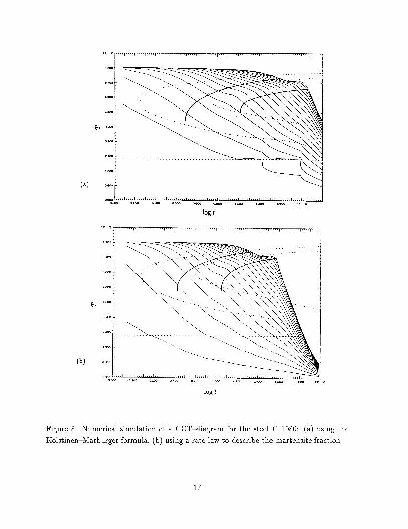
Figure 8: Numerical simulation of a CCT{diagram for the steel C 1080: (a) using the
Koistinen{Marburger formula, (b) using a rate law to describe the martensite fraction.
17
0
20
40
60
80
100
0 8 16 24 32 40
Mar
tens
ite (
%)
Distance from quenched end (1/16 in. units)(b)
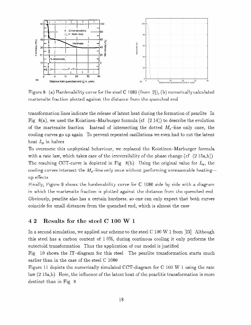
Figure 9: (a) Hardenability curve for the steel C 1080 (from [2]), (b) numerically calculated
martensite fraction plotted against the distance from the quenched end.
transformation lines indicate the release of latent heat during the formation of pearlite. In
Fig. 8(a), we used the Koistinen{Marburger formula (cf. (2.14)) to describe the evolution
of the martensite fraction. Instead of intersecting the dotted Ms{line only once, the
cooling curves go up again. To prevent repeated oszillations we even had to cut the latent
heat Lp in halves.
To overcome this unphysical behaviour, we replaced the Koistinen{Marburger formula
with a rate law, which takes care of the irreversibility of the phase change (cf. (2.15a,b)).
The resulting CCT-curve is depicted in Fig. 8(b). Using the original value for Lp, the
cooling curves intersect the Ms{line only once without performing unreasonable heating{
up e�ects.
Finally, Figure 9 shows the hardenability curve for C 1080 side by side with a diagram
in which the martensite fraction is plotted against the distance from the quenched end.
Obviously, pearlite also has a certain hardness, so one can only expect that both curves
coincide for small distances from the quenched end, which is almost the case.
4.2 Results for the steel C 100 W 1
In a second simulation, we applied our scheme to the steel C 100 W 1 from [23]. Although
this steel has a carbon content of 1.0%, during continous cooling it only performs the
eutectoid transformation. Thus the application of our model is justi�ed.
Fig. 10 shows the IT{diagram for this steel. The pearlite transformation starts much
earlier than in the case of the steel C 1080.
Figure 11 depicts the numerically simulated CCT-diagram for C 100 W 1 using the rate
law (2.15a,b). Here, the in uence of the latent heat of the pearlitic transformation is more
destinct than in Fig. 8.
18
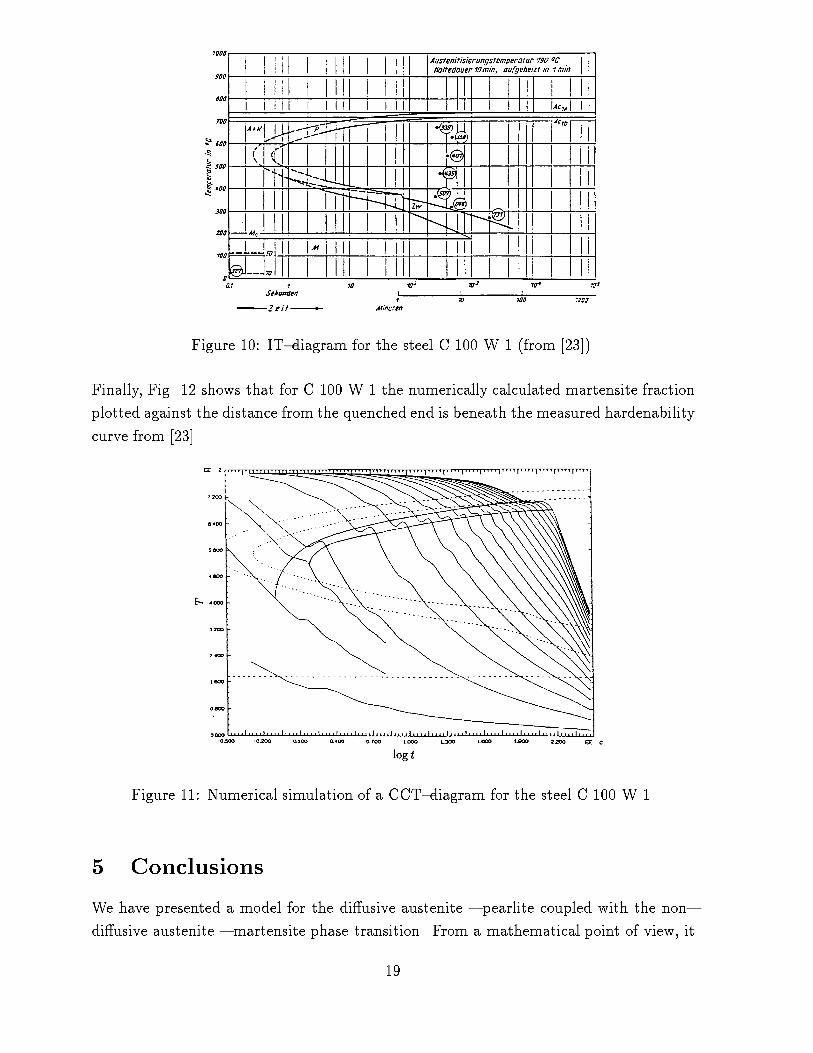
Figure 10: IT{diagram for the steel C 100 W 1 (from [23]).
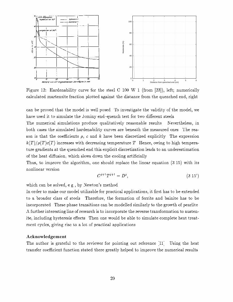
Finally, Fig. 12 shows that for C 100 W 1 the numerically calculated martensite fraction
plotted against the distance from the quenched end is beneath the measured hardenability
curve from [23].
Figure 11: Numerical simulation of a CCT{diagram for the steel C 100 W 1.
5 Conclusions
We have presented a model for the di�usive austenite { pearlite coupled with the non{
di�usive austenite { martensite phase transition. From a mathematical point of view, it
19
0
20
40
60
80
100
0 1 2 3 4 5 6
Mar
tens
ite (
%)
Distance from quenched end (cm)
Figure 12: Hardenability curve for the steel C 100 W 1 (from [23]), left; numerically
calculated martensite fraction plotted against the distance from the quenched end, right.
can be proved that the model is well posed. To investigate the validity of the model, we
have used it to simulate the Jominy end{quench test for two di�erent steels.
The numerical simulations produce qualitatively reasonable results. Nevertheless, in
both cases the simulated hardenability curves are beneath the measured ones. The rea-
son is that the coe�cients �, c and k have been discretized explicitly. The expression
k(T )=�(T )c(T ) increases with decreasing temperature T . Hence, owing to high tempera-
ture gradients at the quenched end this explicit discretization leads to an underestimation
of the heat di�usion, which slows down the cooling arti�cially.
Thus, to improve the algorithm, one should replace the linear equation (3.15) with its
nonlinear version
Cj+1T j+1 = Dj ; (3.15')
which can be solved, e.g., by Newton's method.
In order to make our model utilizable for practical applications, it �rst has to be extended
to a broader class of steels. Therefore, the formation of ferrite and bainite has to be
incorporated. These phase transitions can be modelled similarly to the growth of pearlite.
A further interesting line of research is to incorporate the reverse transformation to austen-
ite, including hysteresis e�ects. Then one would be able to simulate complete heat treat-
ment cycles, giving rise to a lot of practical applications.
Acknowledgement
The author is grateful to the reviewer for pointing out reference [11]. Using the heat
transfer coe�cient function stated there greatly helped to improve the numerical results.
20
References
[1] Agarwal, P. K., Brimacombe, J. K.,MathematicalModel of Heat Flow and Austenite-
Pearlite Transformation in Eutectoid Carbon Steel Rods for Wire, Metall. Trans. B,
12 (1981), 121-133.
[2] American Society for Metals, Atlas of Isothermal Transformation and Cooling Trans-
formation Diagrams, Ohio, 1977.
[3] Andreucci, D., Fasano, A., Primicerio, M., On a Mathematical Model for the Crystal-
lization of Polymers, in: o'Malley, R. E. (Ed..), Proc. ICIAM 1991, SIAM, Philadel-
phia, 1992, 99-118.
[4] Avner, S. H., Introduction to physical metallurgy, McGraw{Hill, Tokyo, 1974.
[5] Avrami, M., J. Chem. Phys., 8 (1940), 812-819.
[6] Bergmann, J., Seeger, T., �Uber neuere Verfahren der Anri�lebensdauervorhersage f�ur
schwingbelastete Bauteile auf der Grundlage �ortlicher Belastungen, Z. Werksto�tech.,
8 (1977), 89-100.
[7] Buza, G., Hougardy, H. P., Gergely, M., Calculation of the isothermal transformation
diagram from measurements with continuous cooling, Steel Res., 57 (1986), 650-653.
[8] Cahn, J. W., Tranformation Kinetics during Continuous Cooling, Acta Met., 4
(1956), 572-575.
[9] Christian, J. W., The Theory of Transformations in Metals and Alloys, Pergamon
Press, Oxford, 1975.
[10] Energie{ und Betriebswirtschaftsstelle des Vereins Deutscher Eisenh�uttenleute, An-
haltszahlen f�ur die W�armewirtschaft in Eisenh�uttenwerken, Verlag Stahleisen mbH,
D�usseldorf, 1968.
[11] Graja, P., M�uller, H., Macherauch, E., Eigenspannungsmessung an Stirnabschreck-
proben in Eigenspannungen, Deutsche Gesellschaft f�ur Metallkunde e.V., Oberursel,
1983.
[12] Hayes, W.J.,Mathematical Models in Materials Science, M. Sc. Thesis, Oxford, 1985.
[13] Hawbolt, E. B., Chau, B., Brimacombe, J. K., Kinetics of Austenite-Pearlite Trans-
formation in Eutectoid Carbon Steel, Metall. Trans. A, 14 (1983), 1803-1815.
21
[14] Hengerer, F., Str�assle, B., Bremi, P., Berechnung der Abk�uhlvorg�ange beim �Ol{ und
Lufth�arten zylinder- und plattenf�ormiger Werkst�ucke aus legiertem Verg�utungsstahl
mit Hilfe einer elektronischen Rechenanlage, Stahl u. Eisen 89 (1969), 641{654.
[15] H�omberg, D., A mathematical model for the phase transitions in eutectoid carbon
steel, IMA J. Appl. Math., 54 (1995), 31{57.
[16] H�omberg, D., Irreversible phase transitions in steel, WIAS Preprint No. 131, 1994.
[17] Hornbogen, E., Skrotzki, B., Fractality and reversibility of ferrous martensite, Steel
Res., 63 (1992), 348{353.
[18] Hougardy, H. P., Darstellung der Umwandlungen f�ur technische Anwendungen und
M�oglichkeiten ihrer Beein ussung in Werksto�kunde Stahl. Bd. 1. Grundlagen,
Springer Verlag, Berlin, 1984, 198-231.
[19] Hougardy, H. P., Yamazaki, K., An improved calculation of the transformation of
steels, Steel Res., 57 (1986), 466-471.
[20] International Organization for Standardization, International Standard 642, Steel {
Hardenability test by end quenching (Jominy test), 1979.
[21] Johnson, W. A., Mehl, R. F., Trans. Amer. Inst. min. metallurg. Eng., Iron Steel
Div., 135 (1939), 416-458.
[22] Koistinen, D. P., Marburger, R. E., A general equation prescribing the extent of
the austenite-martensite transformation in pure iron-carbon alloys and plain carbon
steels, Acta Met., 7 (1959), 59-60.
[23] Max{Planck{Institut f�ur Eisenforschung und der Werksto�ausschuss des Vereins
Deutscher Eisenh�uttenleute, Atlas zur W�armebehandlung der St�ahle, Teil I+II, Ver-
lag Stahleisen mbH, D�usseldorf, 1961.
[24] Scheil, E., Anlaufzeit der Austenitumwandlung, Arch. Eisenh�uttenwes., 12 (1935),
565-567.
[25] Verdi, C., Visintin, A., A mathematical model of the austenite-pearlite transforma-
tion in plain steel based on the Scheil's additivity rule, Acta Metall., 35, No.11 (1987),
2711{2717.
[26] Visintin, A., Mathematical Models of Solid-Solid Phase Transitions in Steel, IMA J.
Appl. Math., 39 (1987), 143-157.
22
[27] Visintin, A., On supercooling and superheating e�ects in phase transitions, Boll.
U.M.I. Analalisi Funzionale e Applicazioni, Serie VI, Vol. V{C, No.1 (1986), 293{
311.
23


![FSL2 - NSV€¦ · 성능그래프 전달율 Graph 동강성 Graph 1 10 10 0 1 000 1 10 D i s t u r b i n g N] Fr e quenc y [H z] Natural Frequency of the System [Hz] 5 20 30 40 50](https://img.pdfslide.net/doc/110x75/602fefeff9ec7e12672393c0/fsl2-eee-eoe-graph-ee-graph-1-10-10-0-1-000-1-10-d-i.jpg)


![FSL2 - NSV · 2020. 5. 8. · FSL2 성능그래프 전달율 Graph 동강성 Graph 10 10 10 0 1 000 1 10 D i s t u r b i n g Fr e quenc y [H z] Natural Frequency of the System [Hz]](https://img.pdfslide.net/doc/110x75/60ab64b452e9e65ca84c7dd9/fsl2-2020-5-8-fsl2-eee-eoe-graph-ee-graph-10-10.jpg)