Embed Size (px)
Citation preview
An XMM-ESAS Update
Steve SnowdenNASA/Goddard Space Flight Center
EPIC Operations and Calibration Meeting - BGWGPalermo - 11 March 2007
With plenty of help from
Kip Kuntz
NASA/Goddard Space Flight Center and Johns Hopkins University
Deterministic Modeling
• Use as many known parameters as possible rather than relying on local background determinations and blank-sky background data sets – which won’t work for cosmic background studies
• E.g., FWC Data, RASS, Soft Proton distribution, Archived Observation Data Sets
Step 1 – Filter the Data and Extract Spectra• Nearly any reasonable method will work
• It is quite likely that there will always be residual soft proton contamination so perfection is not required
• Any variations significantly above statistics will be seen in most any band
• XMM-ESAS uses the 2.5-8.5 keV band for the filtering – but the new espfilt task allows the level to be set by the user
• Create a light curve and then a light-curve histogram• Fit a Gaussian to the main peak• Exclude time periods where the count rate is greater than n
times the RMS above the mean of the Gaussian
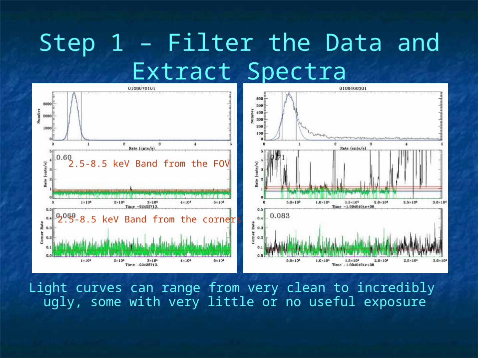
Step 1 – Filter the Data and Extract Spectra
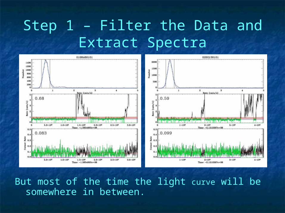
Light curves can range from very clean to incredibly ugly, some with very little or no useful exposure
2.5-8.5 keV Band from the FOV
2.5-8.5 keV Band from the corners
Step 1 – Filter the Data and Extract Spectra
But most of the time the light curve will be somewhere in between.
Step 1 – Filter the Data and Extract Spectra
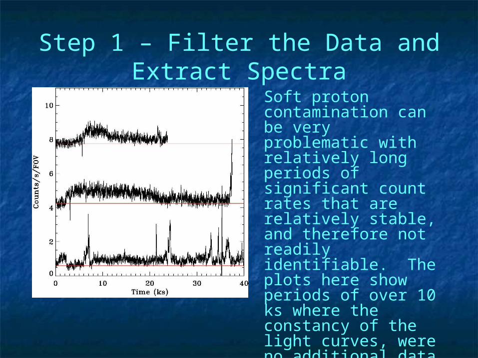
Soft proton contamination can be very problematic with relatively long periods of significant count rates that are relatively stable, and therefore not readily identifiable. The plots here show periods of over 10 ks where the constancy of the light curves, were no additional data available, would suggest that the data were clean.
Step 1 – Filter the Data and Extract Spectra
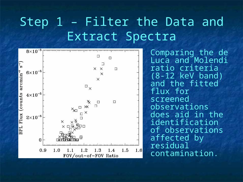
Comparing the de Luca and Molendi ratio criteria (8-12 keV band) and the fitted flux for screened observations does aid in the identification of observations affected by residual contamination.
Step 1 – Filter the Data and Extract Spectra
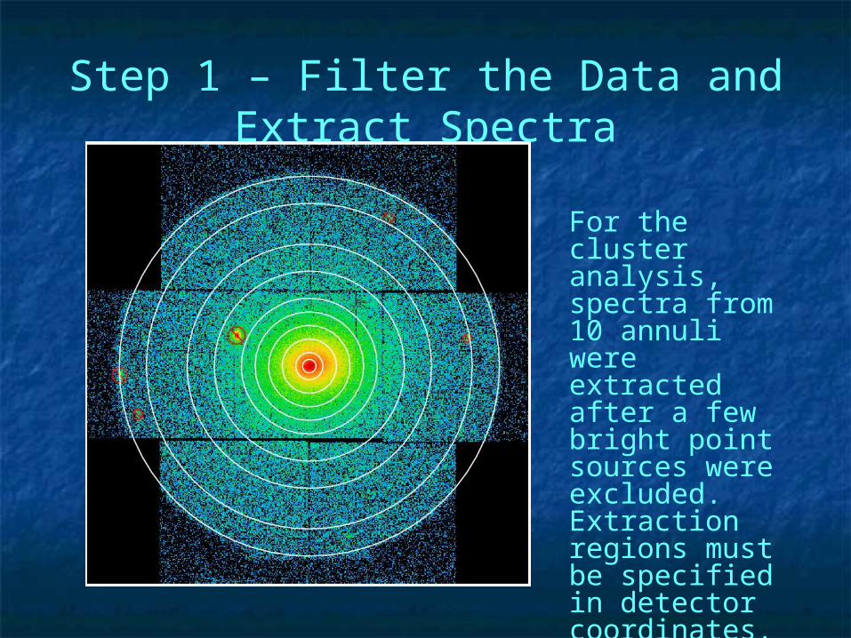
For the cluster analysis, spectra from 10 annuli were extracted after a few bright point sources were excluded. Extraction regions must be specified in detector coordinates.
Step 2 – Model the Quiescent Particle Background
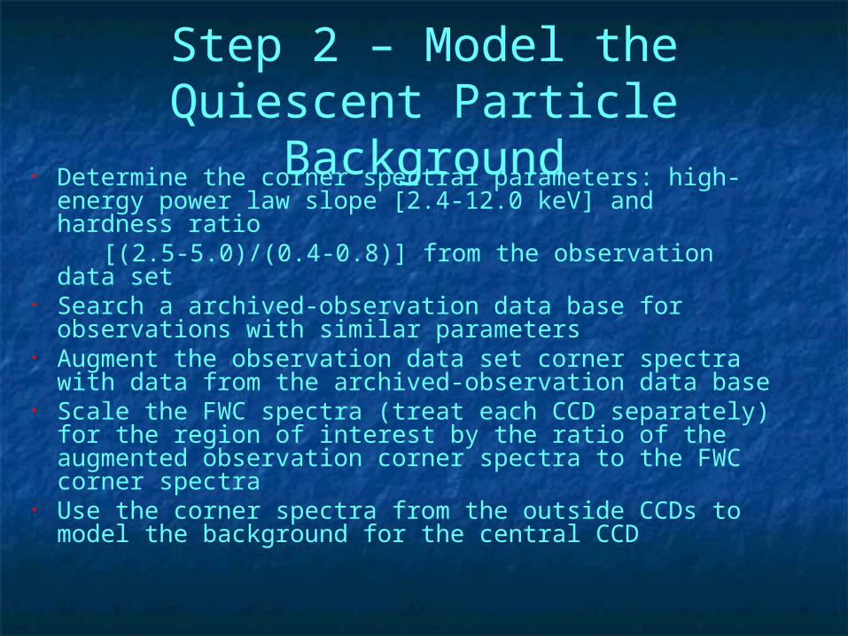
• Determine the corner spectral parameters: high-energy power law slope [2.4-12.0 keV] and hardness ratio
[(2.5-5.0)/(0.4-0.8)] from the observation data set• Search a archived-observation data base for observations with
similar parameters• Augment the observation data set corner spectra with data from
the archived-observation data base• Scale the FWC spectra (treat each CCD separately) for the
region of interest by the ratio of the augmented observation corner spectra to the FWC corner spectra
• Use the corner spectra from the outside CCDs to model the background for the central CCD

Step 2 – Model the Quiescent Particle Background
• Both continuum and line contributions are both position and temporally varying
The mean quiescent particle background spectrum derived from the corner pixel data in two spectral regions: 0.2-5.0 keV and 5-12.5 keV
Step 2 – Model the Quiescent Particle Background
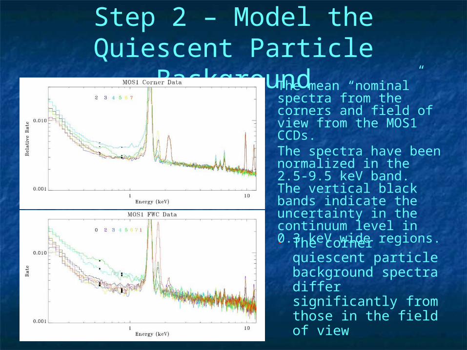
• The corner quiescent particle background spectra differ significantly from those in the field of view
The mean “nominal” spectra from the corners and field of view from the MOS1 CCDs.The spectra have been normalized in the 2.5-9.5 keV band. The vertical black bands indicate the uncertainty in the continuum level in 0.3 keV wide regions.
Step 2 – Model the Quiescent Particle Background
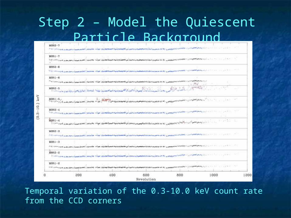
Temporal variation of the 0.3-10.0 keV count rate from the CCD corners
Step 2 – Model the Quiescent Particle Background
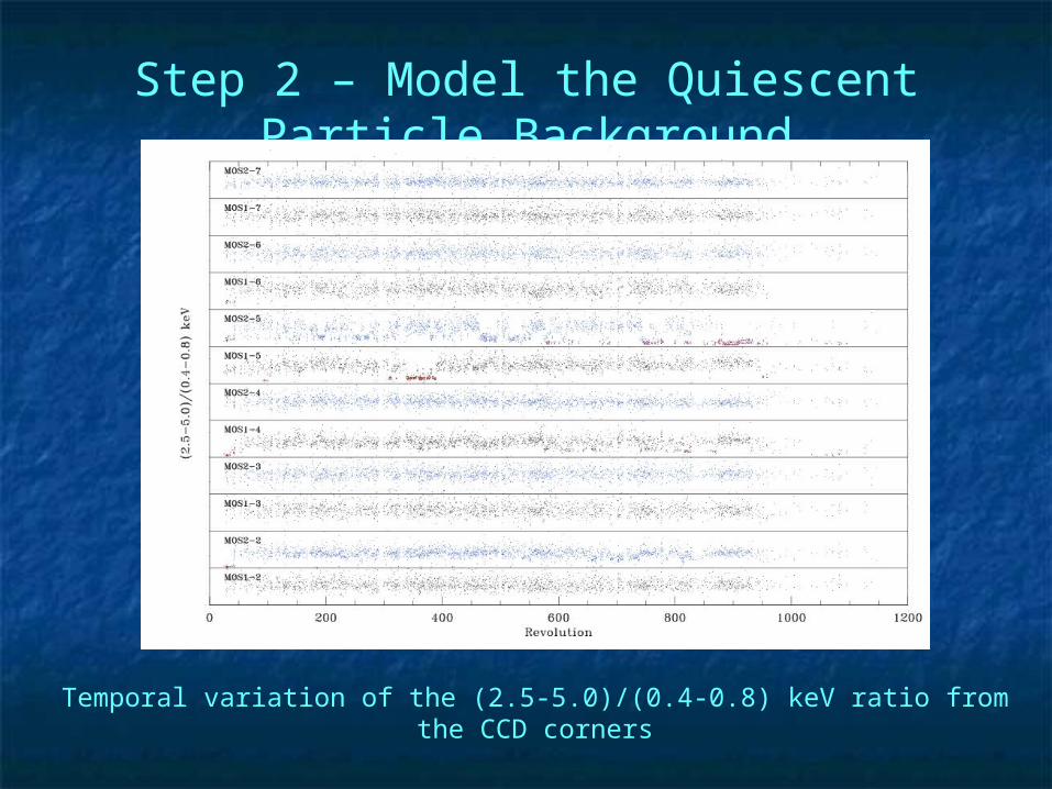
Temporal variation of the (2.5-5.0)/(0.4-0.8) keV ratio from the CCD corners
Step 2 – Model the Quiescent Particle Background
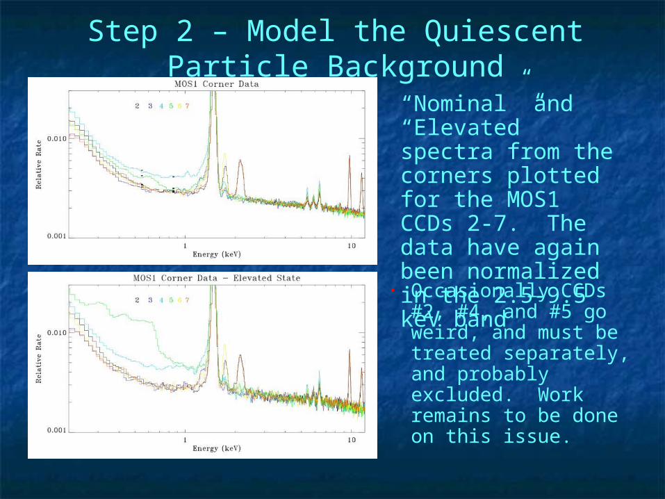
• Occasionally CCDs #2, #4, and #5 go weird, and must be treated separately, and probably excluded. Work remains to be done on this issue.
“Nominal” and “Elevated” spectra from the corners plotted for the MOS1 CCDs 2-7. The data have again been normalized in the 2.5-9.5 keV band
Step 2 – Model the Quiescent Particle Background
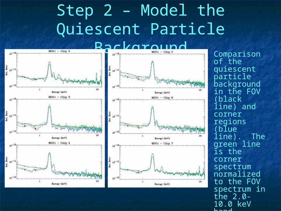
Comparison of the quiescent particle background in the FOV (black line) and corner regions (blue line). The green line is the corner spectrum normalized to the FOV spectrum in the 2.0-10.0 keV band.
Step 2 – Model the Quiescent Particle Background
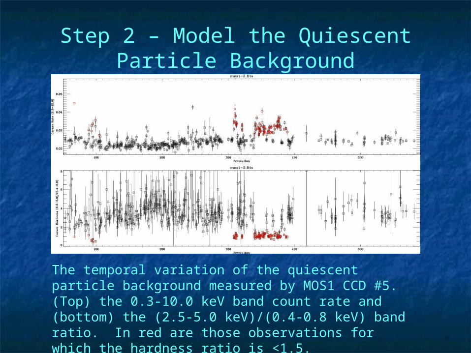
The temporal variation of the quiescent particle background measured by MOS1 CCD #5. (Top) the 0.3-10.0 keV band count rate and (bottom) the (2.5-5.0 keV)/(0.4-0.8 keV) band ratio. In red are those observations for which the hardness ratio is <1.5.
Step 3 – Get the RASS Spectrum for the Area
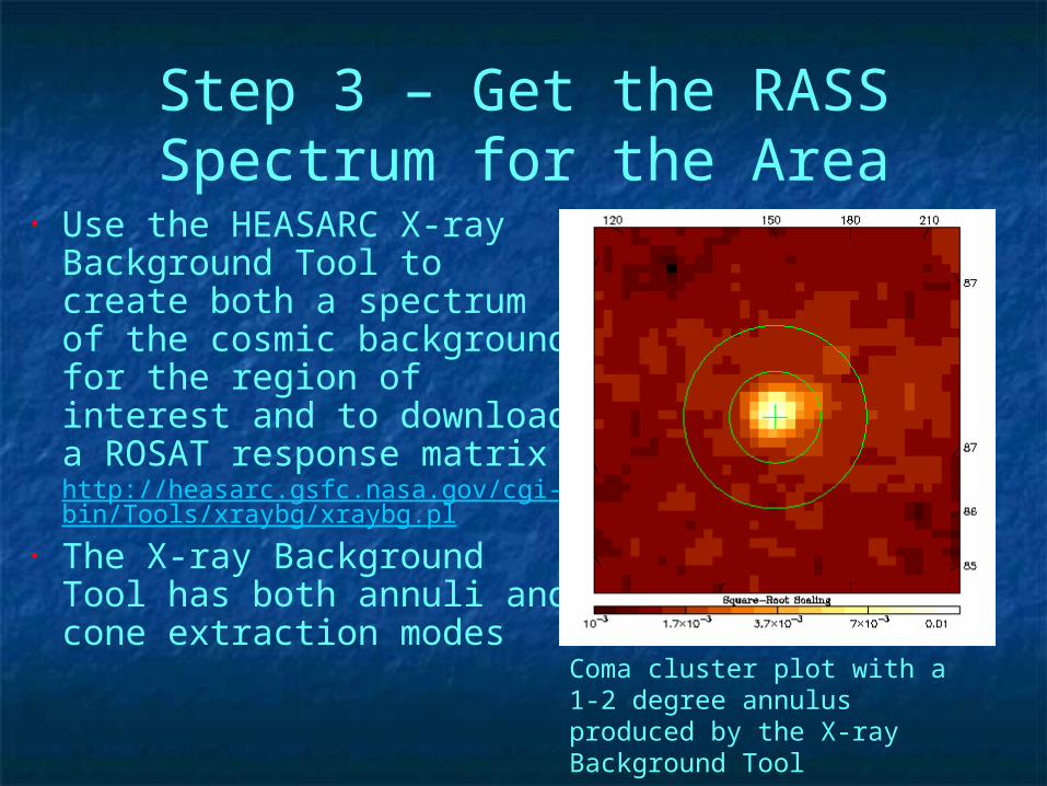
• Use the HEASARC X-ray Background Tool to create both a spectrum of the cosmic background for the region of interest and to download a ROSAT response matrix http://heasarc.gsfc.nasa.gov/cgi-bin/Tools/xraybg/xraybg.pl
• The X-ray Background Tool has both annuli and cone extraction modes
Coma cluster plot with a 1-2 degree annulus produced by the X-ray Background Tool
Step 4 – Fit the Spectrum
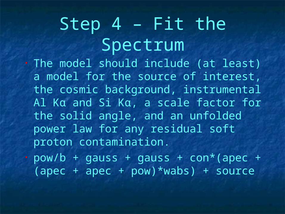
• The model should include (at least) a model for the source of interest, the cosmic background, instrumental Al Kα and Si Kα, a scale factor for the solid angle, and an unfolded power law for any residual soft proton contamination.
• pow/b + gauss + gauss + con*(apec + (apec + apec + pow)*wabs) + source
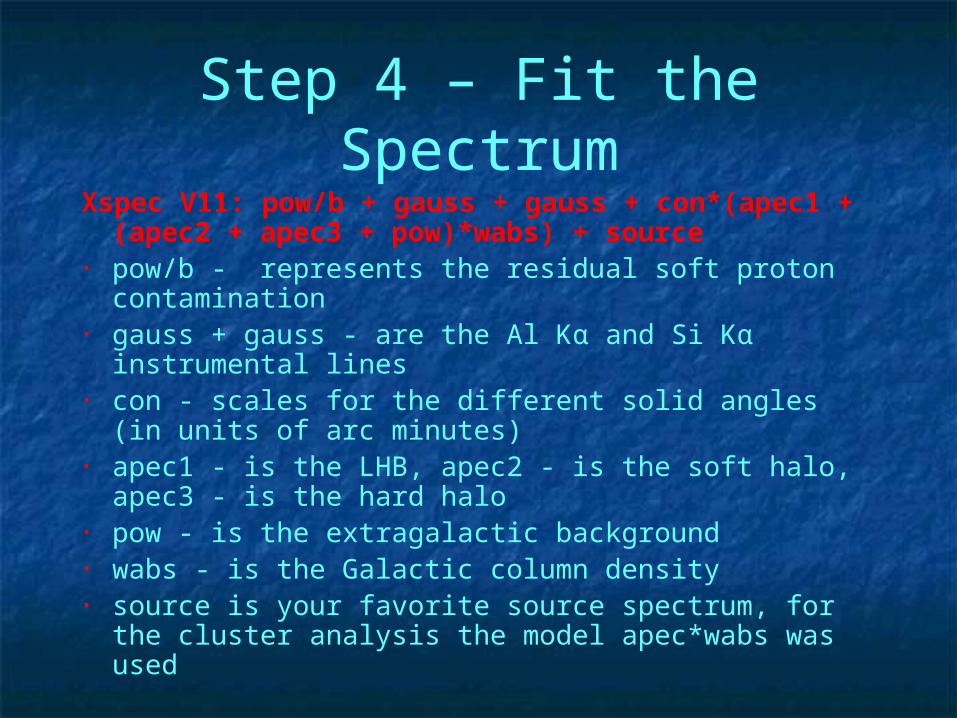
Step 4 – Fit the SpectrumXspec V11: pow/b + gauss + gauss + con*(apec1 + (apec2 +
apec3 + pow)*wabs) + source• pow/b - represents the residual soft proton contamination• gauss + gauss - are the Al Kα and Si Kα instrumental lines• con - scales for the different solid angles (in units of arc
minutes)• apec1 - is the LHB, apec2 - is the soft halo, apec3 - is the
hard halo • pow - is the extragalactic background• wabs - is the Galactic column density• source is your favorite source spectrum, for the cluster
analysis the model apec*wabs was used
Step 4 – Fit the Spectrum
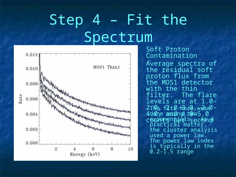
• The fits here were done using two exponentials. As a practical matter, the cluster analysis used a power law. The power law index is typically in the 0.2-1.5 range
Soft Proton ContaminationAverage spectra of the residual soft proton flux from the MOS1 detector with the thin filter. The flare levels are at 1.0-2.0, 2.0-3.0, 3.0-4.0, and 4.0-5.0 counts per second
Step 4 – Fit the Spectrum
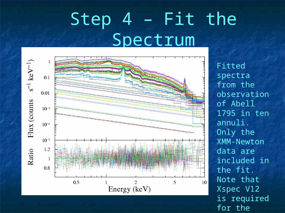
Fitted spectra from the observation of Abell 1795 in ten annuli. Only the XMM-Newton data are included in the fit. Note that Xspec V12 is required for the fitting.
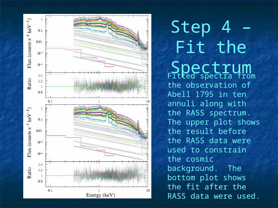
Step 4 – Fit the SpectrumFitted spectra from the observation of Abell 1795 in ten annuli along with the RASS spectrum. The upper plot shows the result before the RASS data were used to constrain the cosmic background. The bottom plot shows the fit after the RASS data were used.
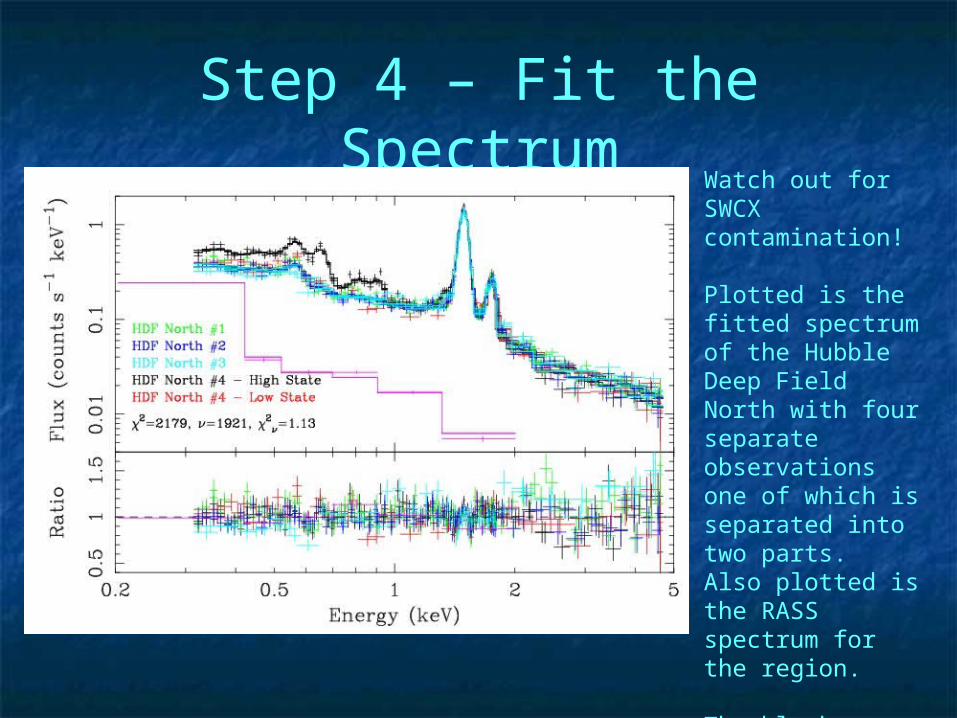
Step 4 – Fit the SpectrumWatch out for SWCX contamination!
Plotted is the fitted spectrum of the Hubble Deep Field North with four separate observations one of which is separated into two parts. Also plotted is the RASS spectrum for the region.
The black curve shows the SWCX contamination.
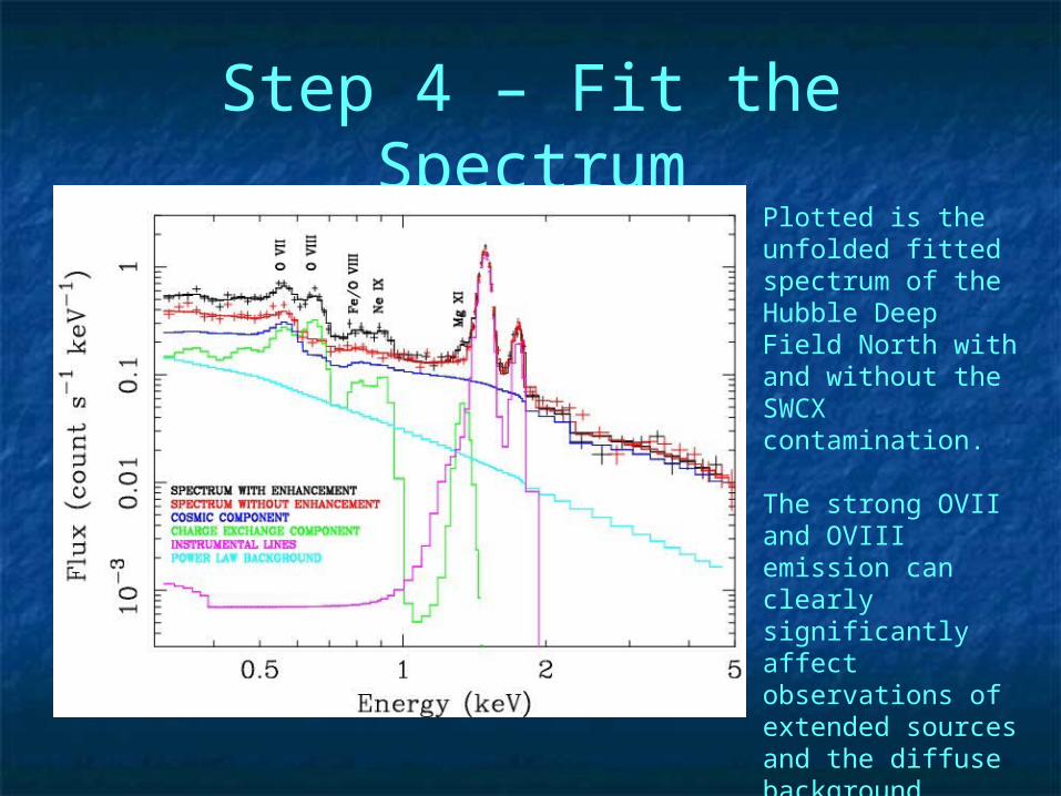
Step 4 – Fit the SpectrumPlotted is the unfolded fitted spectrum of the Hubble Deep Field North with and without the SWCX contamination.
The strong OVII and OVIII emission can clearly significantly affect observations of extended sources and the diffuse background.
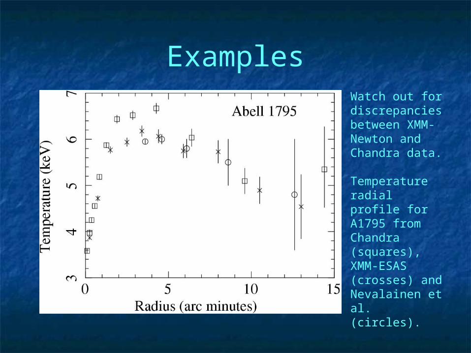
ExamplesWatch out for discrepancies between XMM-Newton and Chandra data.
Temperature radial profile for A1795 from Chandra (squares), XMM-ESAS (crosses) and Nevalainen et al. (circles).
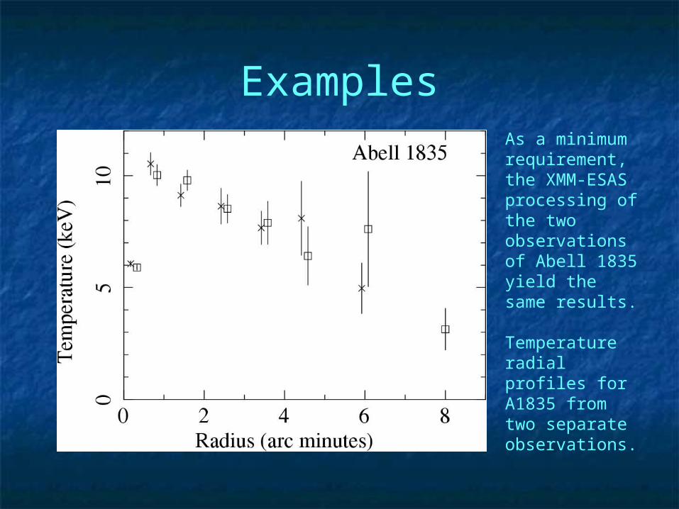
ExamplesAs a minimum requirement, the XMM-ESAS processing of the two observations of Abell 1835 yield the same results.
Temperature radial profiles for A1835 from two separate observations.
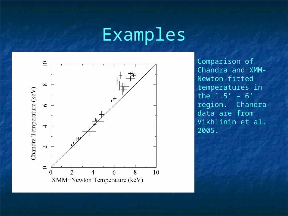
ExamplesComparison of Chandra and XMM-Newton fitted temperatures in the 1.5’ – 6’ region. Chandra data are from Vikhlinin et al. 2005.
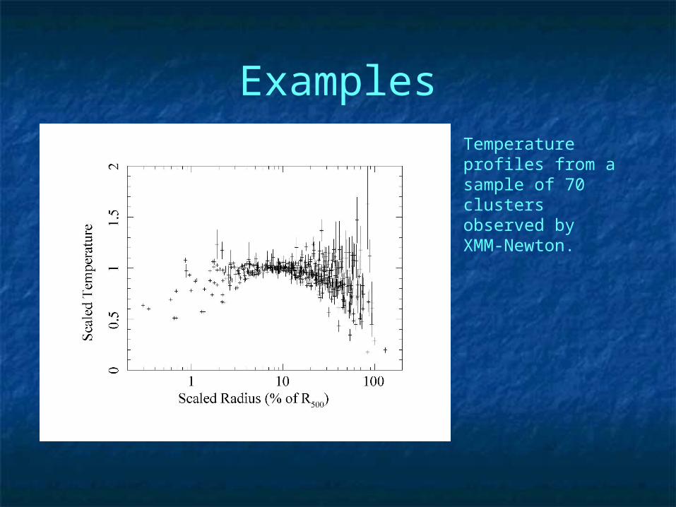
ExamplesTemperature profiles from a sample of 70 clusters observed by XMM-Newton.
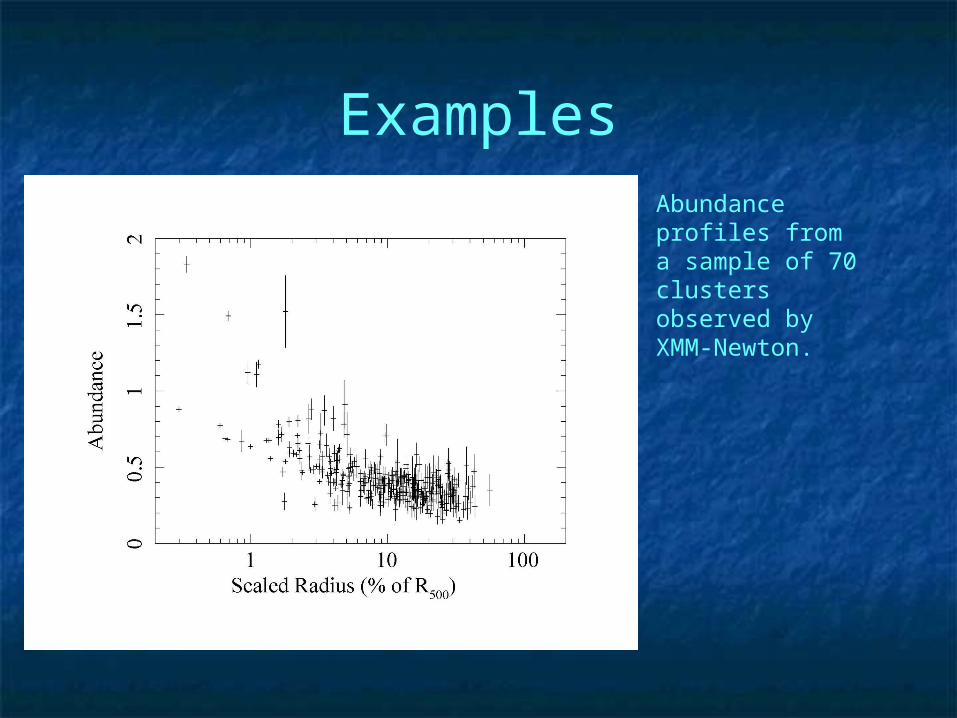
ExamplesAbundance profiles from a sample of 70 clusters observed by XMM-Newton.
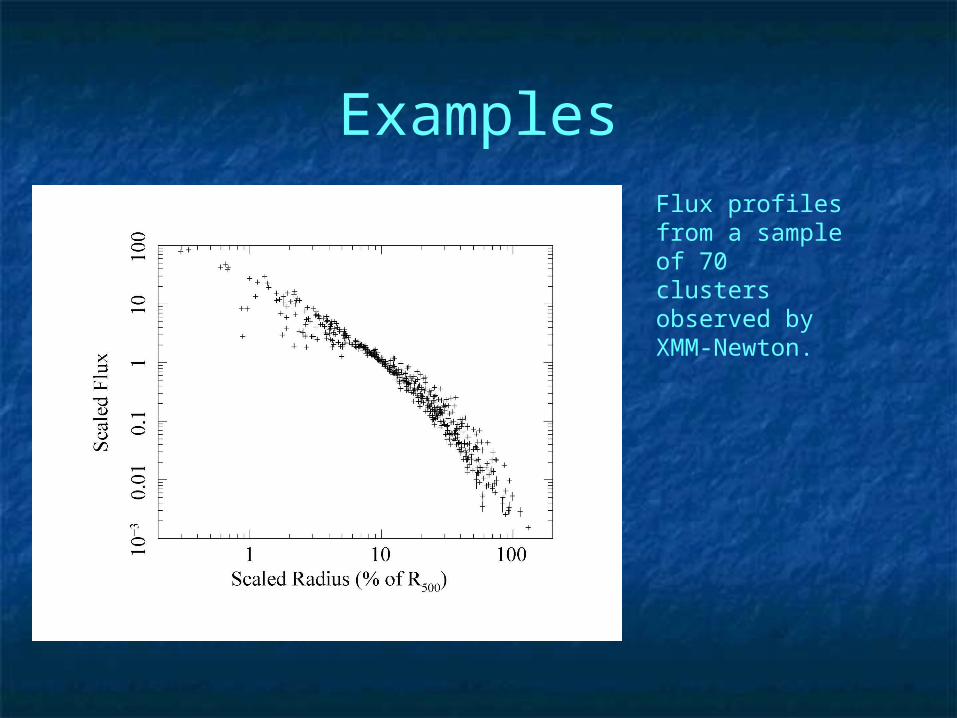
ExamplesFlux profiles from a sample of 70 clusters observed by XMM-Newton.
Images
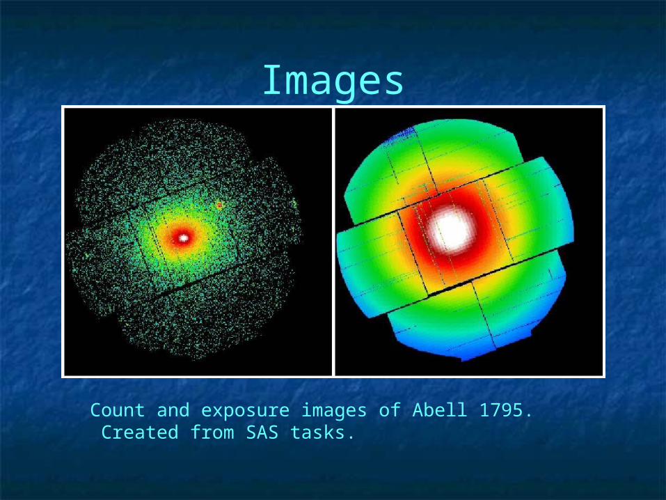
Count and exposure images of Abell 1795. Created from SAS tasks.
Images
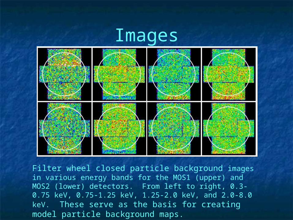
Filter wheel closed particle background images in various energy bands for the MOS1 (upper) and MOS2 (lower) detectors. From left to right, 0.3-0.75 keV, 0.75-1.25 keV, 1.25-2.0 keV, and 2.0-8.0 keV. These serve as the basis for creating model particle background maps.
Images
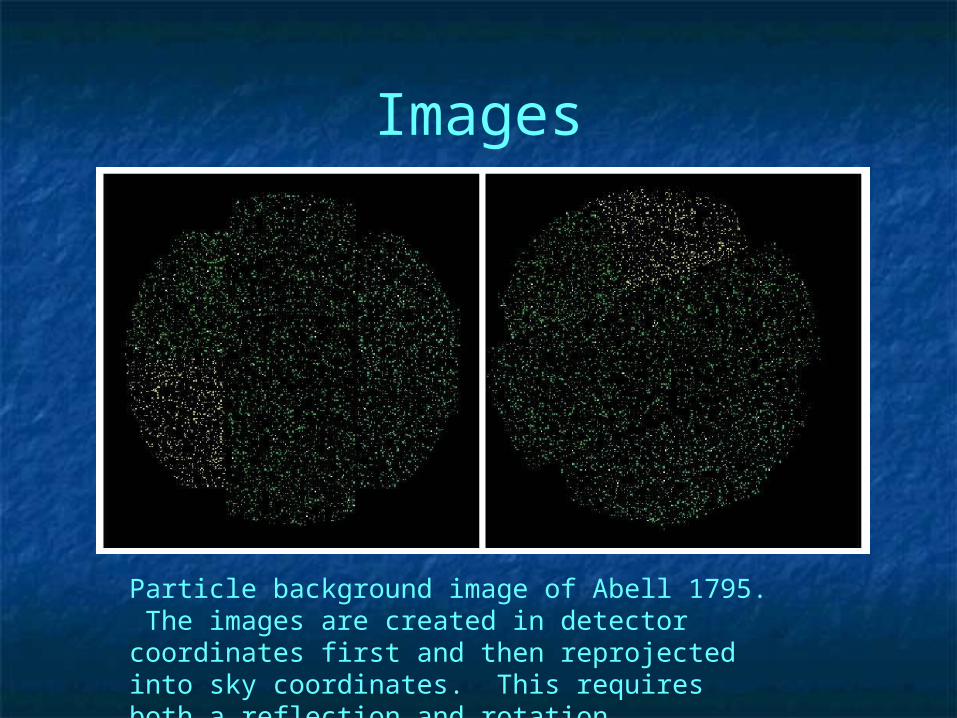
Particle background image of Abell 1795. The images are created in detector coordinates first and then reprojected into sky coordinates. This requires both a reflection and rotation.
Images
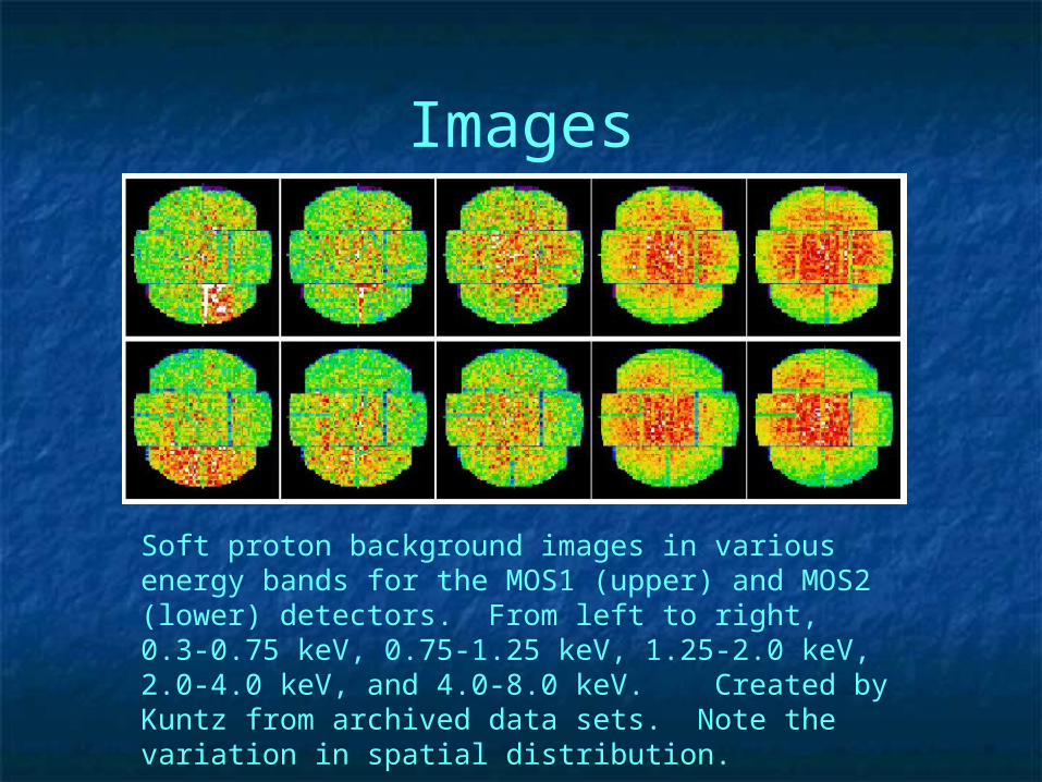
Soft proton background images in various energy bands for the MOS1 (upper) and MOS2 (lower) detectors. From left to right, 0.3-0.75 keV, 0.75-1.25 keV, 1.25-2.0 keV, 2.0-4.0 keV, and 4.0-8.0 keV. Created by Kuntz from archived data sets. Note the variation in spatial distribution.
Images
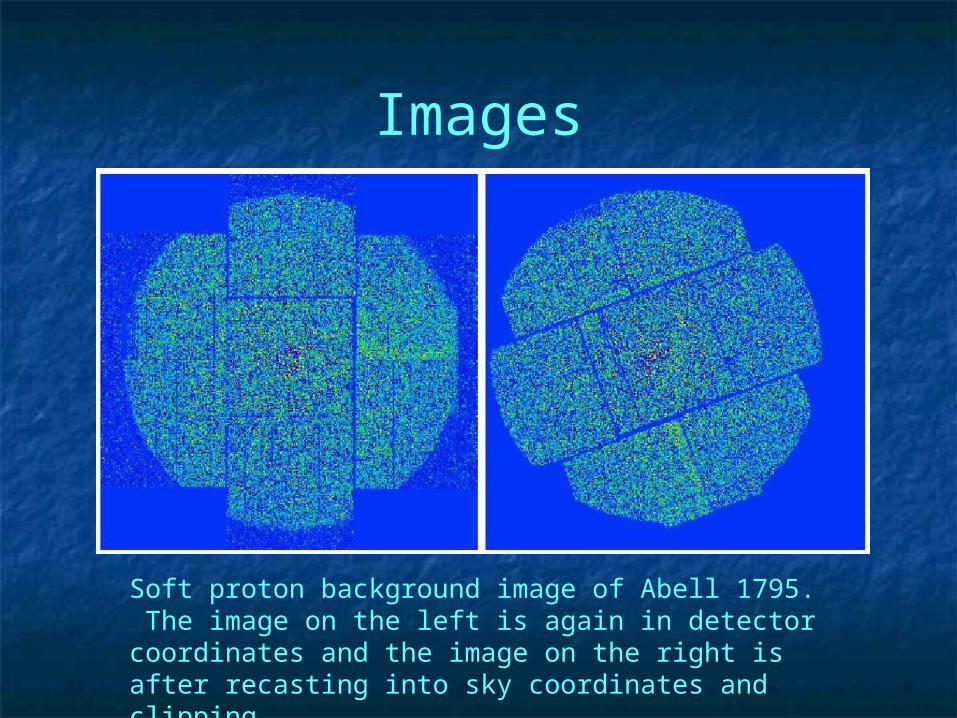
Soft proton background image of Abell 1795. The image on the left is again in detector coordinates and the image on the right is after recasting into sky coordinates and clipping.
Background Subtracted and Exposure Corrected Images
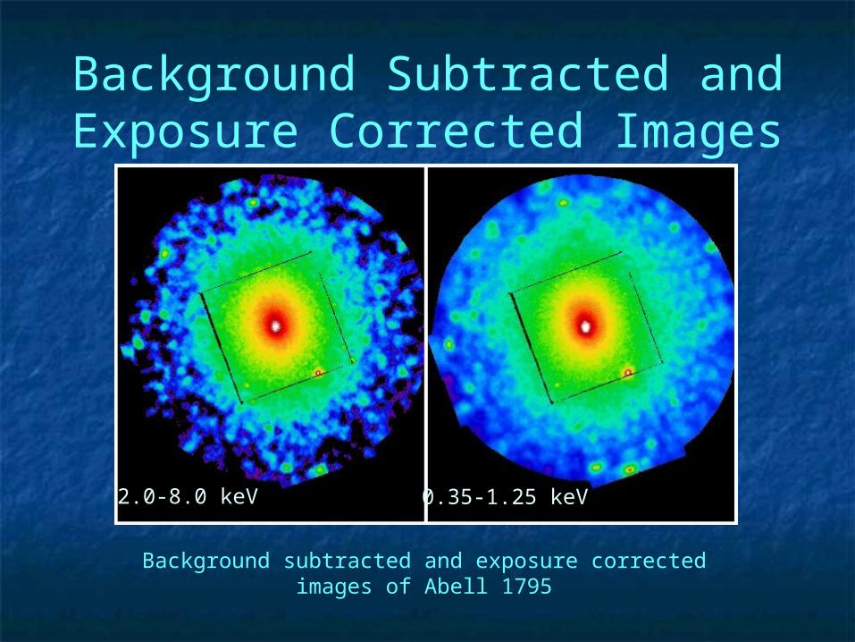
Background subtracted and exposure corrected images of Abell 1795
2.0-8.0 keV 0.35-1.25 keV
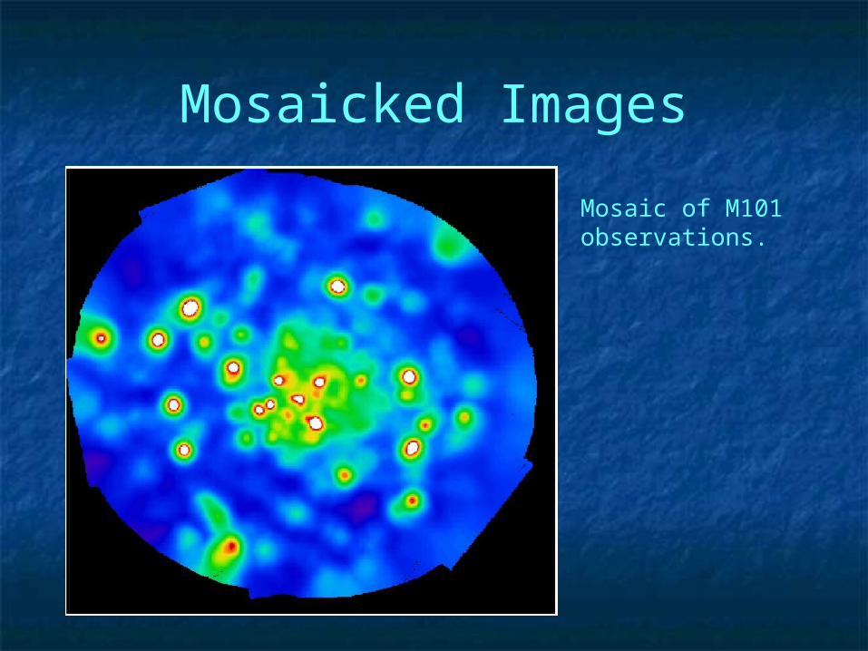
Mosaicked Images
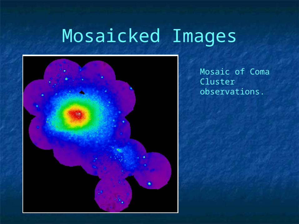
Mosaic of Coma Cluster observations.
Mosaicked Images
Mosaic of M101 observations.