Embed Size (px)
Citation preview
1
Analog and numerical experiments of double subduction systems with 1
opposite polarity in adjacent segments 2
3
Mireia Peral1,2
, Jonas Ruh1,3
, Sergio Zlotnik4, Francesca Funiciello
5, Manel Fernàndez
1, Jaume 4
Vergés1, Taras Gerya
6 5
1) Group of Dynamics of the Lithosphere, Institut de Ciències de la Terra Jaume Almera, ICTJA-6
CSIC, Barcelona, Spain. 7
2) Department of Earth and Ocean Dynamics, Universitat de Barcelona, Barcelona, Spain. 8
3) Structural Geology and Tectonics Group, Geological Institute, Department of Earth Sciences, 9
ETH Zurich, Switzerland. 10
4) Department of Civil and Environmental Engineering, Universitat Politècnica de Catalunya, 11
Barcelona, Spain. 12
5) Laboratory of Experimental Tectonics, Department of Sciences, Università degli Studi Roma 13
Tre, Rome, Italy. 14
6) Institute of Geophysics, Department of Earth Sciences, ETH Zurich, Switzerland. 15
Keypoints 16
• Numerical models of double subduction have been developed to reproduce laboratory 17
experiments and to understand the dynamics of the system. 18
• The interaction between the induced mantle flows slows down the evolution of the 19
system and generates additional deformation of plates. 20
• In the horizontal plane mantle flow forms four toroidal cells with symmetry axes that 21
rotate during trench retreat. 22

2
Keywords: mantle flow/plate interaction, numerical and analog models, trench retreat, trench 23
curvature, plate deformation. 24
3
ABSTRACT 25
In this work we study the dynamics of double subduction systems with opposite polarity in 26
adjacent segments. A combined approach of numerical and analog experiments allows us to 27
compare results and exploit the strengths of both methodologies. High-resolution numerical 28
experiments complement laboratory results by providing quantities difficult to measure in the 29
laboratory such as stress state, flow patterns and energy dissipation. Results show strong 30
asymmetries in the mantle flow that produce in turn asymmetries in the trench and in the 31
downgoing slab deformation. The mantle flow pattern varies with time; the toroidal cells 32
between the plates evolve until merging into one unique cell when the trenches align. In that 33
moment the maximum upward flow is observed close to the trenches. The interaction between 34
the mantle flow produced by each subducting plate makes the rollback processes slower than in a 35
single subduction case. This is consistent with the observed energy dissipation rate that is smaller 36
in the double subduction system than in two single subductions. Moreover, we provide a detailed 37
analysis on the setup and boundary conditions required to numerically reproduce the analog 38
experiments. Boundary conditions at the bottom of the domain are crucial to reproduce their 39
analog counterparts. Numerical results are compared to natural examples of multi-slab 40
subduction systems in terms of upper mantle seismic anisotropy, relative trench-retreat velocities 41
and composition of subduction-related magmatism. 42
43
1 INTRODUCTION 44
The study of subduction zones is of prime importance since they play an essential role as main 45
driving mechanism for plate tectonics and mantle dynamics [Coltice et al., 2019]. A large part of 46
4
the current subduction zones, where a single oceanic plate descends beneath another continental 47
or oceanic plate, are associated with nearly linear trenches that extend over distances of some 48
thousands of kilometers (e.g., Aleutians, Peru-Chile, Kermadec-Tonga, Japan–Kurile, Java–49
Sunda). Mantle dynamics in such subduction zones is dominated by poloidal cells induced by the 50
entrained flow beneath the slab and the corner flow produced by the down dip of the slab. 51
Toroidal cells around the slab edges can be developed in response to the return mantle flow 52
associated with the trench migration [Gable et al., 1991]. 53
This mantle flow pattern can be largely modified by the presence of vertical and horizontal slab 54
tears and slab fragmentation [e.g., Liu and Stegman, 2012; Long, 2016; Magni et al., 2017]. 55
Furthermore, in settings where oceanic plates are highly segmented, subduction is commonly 56
characterized by very arcuate trenches of limited extent showing different slab dip orientations. 57
Indeed, we can observe double subduction systems with parallel trenches with inward-dipping 58
polarity as in Luzon [Bautista et al., 2001], outward-dipping polarity as in Molucca Sea [Zhang 59
et al., 2017], or same-dipping polarity as in Philippine Sea [Faccenna et al., 2018]. In addition, 60
there are subduction systems characterized by two adjacent slabs retreating in opposite directions 61
as in Taiwan [Lallemand et al., 2001], New Zealand [Lamb, 2011], the Western Mediterranean 62
[Vergés and Fernàndez, 2012] and the Alps-Apennine junction in Italy [Vignaroli et al., 2008]. 63
All these complex subduction systems can modify the sub-lithospheric mantle flow generating 64
seismic anisotropy and the geochemical signature of subduction-related magmatism [e.g., 65
Faccenda and Capitanio, 2013; Ma et al., 2019; Magni, 2019]. 66
The dynamics of double subduction systems have been investigated by a wealth of numerical and 67
analog experiments involving different configurations [e.g., Di Leo et al., 2014; Holt et al., 2017; 68
Mishin et al., 2008; Pusok and Stegman, 2019]. In particular, subduction systems characterized 69
5
by two adjacent slabs retreating in opposite directions have been tested with 3D numerical 70
[Király et al., 2016] and analog experiments [Peral et al., 2018]. Whereas Király et al. [2016] 71
focused on the interactions between the return flows generated by the respective retreating slabs, 72
Peral et al. [2018] investigated plate deformation and variations in trench retreat velocities. 73
Although both models use similar geometries and share main outcomes, differences in the model 74
setup make it difficult to compare them. 75
Combining computational and laboratory models of the same geodynamic process may help 76
understanding its dynamic evolution by complementing each method’s weaknesses and strengths 77
[e.g., Mériaux et al., 2018; Panien et al., 2006]. While laboratory experiments provide the 78
physical realism and high temporal and geometrical resolution, numerical models allow for fully 79
controlling and quantifying physical parameters, as velocity and stress, which cannot be directly 80
obtained from laboratory experiments. This said, the numerical reproduction of laboratory results 81
in terms of temporal evolution of the subduction process, trench curvature, and slab geometry 82
helps identifying and understanding boundary conditions, rheological behavior and other effects 83
in analog experiments. 84
Only a couple of studies compare analog and numerical experiments of single-plate subduction 85
and elaborate differences and similarities obtained by the different methods [Mériaux et al., 86
2018; Schmeling et al., 2008]. Schmeling et al. [2008] pointed out the importance of a zero-87
density weak top layer to simulate the free surface behavior when trying to reproduce laboratory 88
experiments numerically. More recently, Mériaux et al. [2018] presented 3D numerical models 89
with the objective of reproducing single-plate subduction laboratory experiments. They proposed 90
that surface tension effects of the syrup representing the mantle material in analog experiments 91
may affect the resulting trench retreat velocity and flank stability of subducting plates. 92
6
Here, we perform numerical models aiming to reproduce analog experiments of complex double 93
subduction systems as recently published in Peral et al. [2018]. In this regard, the geometrical 94
setup and material parameters have been chosen to best represent values applied in the 95
laboratory. The main objective of our work is to better understand the evolution of small-scale 96
subduction systems with opposite polarity in adjacent segments by determining the relevant 97
physical parameters that characterize these processes. The study is divided into three main 98
objectives: 1) Testing the effects of boundary conditions, rheology and plate thickness on the 99
evolution of single- and double-plate subduction systems to evaluate how the assumed 100
simplifications in numerical models can affect the results. Furthermore, those results also help to 101
identify the nature of analog boundary conditions and rheological uncertainties. 2) 102
Establishing a reference subduction system with opposite polarity to analyze plate deformation 103
and mantle flow interaction by quantifying velocities, stresses and forces within such systems. 3) 104
Comparing numerical results to natural systems and interpreting the geological consequences 105
during the evolution of these subduction systems in terms of trench retreat velocities, plate 106
deformation, magmatism, and seismic anisotropy. 107
108
2 METHODOLOGY 109
2.1 Analog model 110
Laboratory experiments presented by Peral et al. [2018] were performed in a plexiglass tank 111
with dimensions of 150 x 150 x 50 cm3. Materials consist of both linear viscous glucose syrup 112
and silicone putty representing the upper mantle and subducting plates, respectively. Subduction 113
is driven by a density difference between the initially floating plates and the mantle material. All 114
7
material parameters and respective scaling are described in Table 1. Among the models included 115
in Peral et al. [2018] we have chosen the double subduction configuration consisting of 10 cm 116
wide plates, and the single subduction configuration with a 30 cm wide plate for comparison to 117
numerical experiments. The length of the plates (l) measures 30 cm and the distance between the 118
trailing edges (s) is 39 cm (Fig. 1). The plates are fixed at their trailing edge and the upper/lower 119
mantle boundary is simulated by placing a fixed base at 11 cm depth. Subduction is initiated by 120
manually pushing down the leading edge of the plates into the syrup to about 3 cm depth. For 121
more details about the analog experiments, we refer to Peral et al. [2018]. 122
2.2 Numerical model 123
The numerical counterparts of single plate and double plate subduction models with opposite 124
polarity have been performed by a three-dimensional code based on the finite difference method 125
with a fully-staggered Eulerian grid and freely advecting Lagrangian markers [I3ELVIS; Gerya, 126
2009; Gerya and Yuen, 2007]. Similar to the analog experiments we applied a linear (Newtonian) 127
rheology. The numerical model solves the equation for conservation of mass assuming 128
incompressibility 129
𝜕𝑣𝑖
𝜕𝑥𝑖= 0 (1) 130
and conservation of momentum (Stokes equation) 131
𝜕𝜏𝑖𝑗
𝜕𝑥𝑗−
𝜕𝑃
𝜕𝑥𝑖= 𝜌𝑔
𝑖 (2) 132
where vi are the velocities in x-, y- and z- direction, xi are the spatial coordinates, P is the 133
dynamic pressure, 𝜌 is the density, and gi is the gravitational acceleration. Deviatoric stresses are 134
defined by 135
8
𝜏𝑖𝑗 = 𝜂 (𝜕𝑣𝑖
𝜕𝑥𝑗+
𝜕𝑣𝑗
𝜕𝑥𝑖) (3) 136
where η denotes the viscosity. 137
The governing equations are solved with an OpenMP-parallelized multigrid solver running on 16 138
threads. The duration of single time steps is capped to ensure that no marker moves further than 139
1/10 of a nodal cell size, with a maximal value of one minute (average time steps defined by 140
marker movement are around four seconds). Numerical experiments needed around two weeks to 141
complete. Respectively, wall time of conducted experiments average out at around 5400 hours 142
(runtime multiplied by amount of threads). The nodal resolution of the models depends on the 143
size of the computational domain (Table 2). All experiments initially contain eight Lagrangian 144
markers per nodal cell. Marker properties are interpolated to nodes by an arithmetic averaging 145
scheme, whereas the velocity field calculated on the Eularian grid is back-interpolated onto the 146
markers by applying the fourth-order Runge-Kutta method. 147
Model setup 148
Geometrical and physical parameters of numerical models have been chosen to best reproduce 149
analog experiments from which we have selected those with narrow plates in the double 150
subduction system and wide plates for the single plate system. All experiments with only one 151
plate exhibit a vertical plane of symmetry parallel to the subduction direction in the middle of the 152
plate. Technically, these experiments could have been conducted in a half space. However, we 153
decided to apply full box sizes for all experiments for a better visual comparison to analogue and 154
asymmetric numerical experiments. To assess boundary effects acting on the subduction system, 155
three Eulerian box sizes have been considered since the smaller the size of the box, the higher the 156
numerical resolution. Large, intermediate and small boxes measure 150 x 150 cm2 (model N1), 157
9
80 x 80 cm2 (model N2) and 30 x 40 cm
2 (model N3) in horizontal directions, respectively. The 158
largest box model corresponds to the real dimensions of the tank used in the laboratory 159
experiment [Peral et al., 2018]. Due to the relatively large cell size in model N1, plates are 160
initially spaced 2 cm while in the rest of the models the initial lateral distance is of 1 cm, 161
corresponding to the separation that is observed in the laboratory experiments immediately after 162
subduction initiation. All models have a height of 12 cm. The initial distribution of markers is 163
characterized - from bottom to top - by 11 cm of mantle and 1 cm of “sticky-air”, which is a low-164
density, low-viscosity phase imposing low shear stresses along its interface with the mantle/plate 165
and allowing the system to develop a surface topography. The top boundary of the sticky-air 166
layer is no-slip. We have also tested models with free-slip top boundary conditions showing very 167
similar results though consuming a much longer computation time. 168
The density of the mantle material is 1445 kg/m3, the plates have a density of 1505 kg/m
3 and the 169
“sticky-air” layer has a density of 1 kg/m3 (Table 2). All models but one exhibit a linear viscous 170
rheology for both plates and mantle (Table 2). Plates have an initial thickness of 1 cm, 1.2 cm or 171
1.35 cm and are located at the top of the mantle, in contact with the “sticky-air” layer (Fig. 1). 172
Plate lengths are 30 cm with a width of 10 cm for double plate and a width of 10 cm or 30 cm for 173
single-plate models (Table 2). Plates are fixed at their trailing end by predefined null nodal 174
velocity in all directions at a distance of 39 cm to each other parallel to the plate extent (Fig. 1). 175
To initiate density-driven subduction, a small slab perturbation is initially imposed at their tips 176
where the slab penetrates 3 cm into the mantle at 45° dip angle. One additional model has been 177
conducted with a non-linear, strain-rate dependent viscosity for the subducting plate (model 178
N15). The non-linear viscosity is calculated by 179
10
𝜂𝑙 = 𝜂0 ∙ 𝜀�̇�𝐼(
1
𝑛−1)
(4) 180
where η0 denotes the reference viscosity, n is the power-law exponent and ͘εII the second invariant 181
of the strain-rate tensor (Table 2). 182
Subduction of the plate(s) in the numerical models is dynamically self-consistent in the sense 183
that it is driven by density contrast only and no material flux is allowed into and out of the model 184
domain. Lateral and bottom boundary conditions are variably prescribed as no-slip or free-slip 185
(zero shear stresses along boundary) to test their effect on mantle flow and subduction retreat 186
(Table 2). 187
188
3 COMPARING ANALOG - NUMERICAL EXPERIMENTS 189
Preliminary numerical models have been run reproducing the laboratory conditions to better 190
understand how the numerical/analog modeling constraints affect the final results in the natural 191
prototype rather than to the laboratory experiments itself. A 3-steps parametric study has been 192
performed allowing to design the optimum numerical experiment to study the double subduction 193
systems: First, numerical models of double subduction systems with 10 cm wide plates were 194
designed to test the effects of variable model domain size. Second, the importance of applied 195
numerical boundary conditions was investigated. Finally, numerical models with a single 30 cm 196
wide plate were conducted to reveal the effects of plate stiffness by varying plate viscosity and 197
thickness. Geometric and physical parameters of all presented models are listed in Table 2. 198
Results are described taking into account the different phases of the evolution of a subduction 199
system with opposite polarity in adjacent segments described in Király et al. [2016]: i) initial 200
11
stage corresponding to the evolution of the system until plates reach the base of the upper mantle 201
(phase 1); ii) approaching trenches, starting with the acceleration of slab rollback after the slabs 202
interact with the lower mantle and finishing when trenches intersect, i.e. are aligned to each other 203
(phase 2); and iii) diverging trenches, spanning from trench intersection until subduction 204
completes (phase 3). We define trench intersection as the transition from phase 2 to phase 3. 205
3.1 Influence of model domain size 206
Numerical models with different box sizes show similar plate geometries during the different 207
phases of subduction (Fig. 2). Phase 1 is not shown in this section as the trenches are too far 208
from each other to produce any interaction between plates. Phase 2 shows that plates tend to 209
approach each other, this effect being more intense for the medium and small box experiments. 210
In phase 3, subduction continues and the slabs show a flattened asymmetric shape lying on the 211
bottom of the model. This asymmetric deformation is less intense in model N1, where plates are 212
initially more separated. The flow pattern at 6 cm depth from the top of the model domain is 213
similar in all models (Fig. 2), though the radius of the toroidal flow is smaller as the box size 214
decreases. The maximum mantle velocities (~1.4 mm/min) at this depth are registered in front of 215
the trench and behind the slab during the entire subduction process. 216
Figure 3 illustrates the amount of trench retreat versus time for numerical experiments with 217
different box sizes in comparison to the reference analog experiment. Trenches of the analog 218
experiment retreat with a roughly linear trend (orange and black points in Fig. 3 with their linear 219
regression as black line). In contrast, curves of numerical experiments show a concave trend 220
indicating a slight acceleration during phase 3 that is most evident in model N2 (80 x 80 cm2) 221
(Fig. 3). 222
12
3.2 Influence of applied boundary conditions 223
We first analyze the role of the conditions applied to the lateral boundaries of the model domain. 224
Figure 4 illustrates the temporal evolution of trench retreat of models with free-slip (N1, N2 and 225
N3) and no-slip (N4, N5 and N6) conditions. Applying free-slip conditions allows the mantle 226
material to move along the lateral walls of the box without resistance. Contrariwise, no-slip 227
lateral boundary conditions prevent lateral flow on the surface of the walls. There are no 228
noticeable differences in the resulting trench retreat related to these two end-member boundary 229
conditions for models with box size of 150 x 150 cm2 and 80 x 80 cm
2. However, models N3 and 230
N6 (box size 40 x 30 cm2) show a measurable offset with free-slip boundaries resulting in a 231
slightly faster trench retreat (Fig. 4). 232
Secondly, we explore the effects of applying a free-slip or no-slip boundary condition at the 233
bottom of the model domain (Fig. 5). Laboratory experiments show that subducted plates when 234
reaching the basal plate, at least to a certain extent, deform and move horizontally. This 235
observation requires testing different bottom boundary conditions for the numerical counterpart 236
[Peral et al., 2018]. A double subduction model with no-slip boundary condition at the bottom 237
implies zero horizontal velocity for the mantle and the slab material at the base of the model 238
domain. Therefore, lateral movement and stretching of the plate lying on the floor of the model is 239
restricted (Fig. 5a). On the other hand, free-slip boundary conditions at the bottom allow the 240
slabs to stretch in horizontal directions and slabs can move laterally along the bottom boundary 241
depending on the resulting velocities (Fig. 5b). Trench retreat velocities are up to 15% higher for 242
free-slip than for no-slip conditions and the toroidal mantle flow produces a lateral movement of 243
both slabs that is not observed for the no-slip models. 244
13
3.3 Influence of plate rheology and plate thickness 245
Previous laboratory experiments of single and double subduction have shown that the trenches of 246
subducting plates exhibit a more intense curvature than numerical models when applying the 247
measured spatial and rheological parameters (Fig. 6a, 6b). This effect, which is more pronounced 248
for wider plates, raises the question whether the rheology of the plates and the mantle differ for 249
laboratory and numerical models. Therefore, a series of numerical models with a 30 cm wide 250
single plate was conducted to test the effects of plate rheology and thickness on the subduction 251
process and particularly on the trench curvature (see Table 2 and Fig. 6). 252
Results show that the trench curvature, defined as the ratio between the chord and the sagitta of 253
the circular segment delineated by the trench [Peral et al., 2018], decreases and the deformation 254
and stretching of the slab increases with a decreasing viscosity ratio between the lithosphere and 255
the mantle (𝛾 = 𝜂𝑙/𝜂𝑚). Reducing the viscosity ratio from a reference value γ = 195 to γ = 100 is 256
not sufficient to reproduce the slab deformation observed in the laboratory experiment (Fig. 6c). 257
However, reducing at the same time the viscosity ratio to γ = 100 and the plate thickness to 1.2 258
cm maintains the trench curvature showing a more pronounced slab deformation (Fig. 6d). A 259
similar effect has been observed for a non-Newtonian plate viscosity (Fig. 6e). The numerical 260
model that best represents the laboratory experiment in terms of plate deformation (slab 261
deformation and trench curvature) is obtained by reducing the plate thickness to 1.0 cm (Fig. 6f). 262
However, the time evolution of this model (model N11) differs notably from that performed in 263
the laboratory. 264
3.4 Reference model for the double plate numerical experiment 265
14
Reducing the computational domain allows to increase the model resolution without increasing 266
the computational cost and therefore to simulate the laboratory experiment with more spatial 267
accuracy. Regarding the size of the computational domain, negligible differences in terms of 268
plate geometry and trench retreat velocity are obtained when reducing the numerical domain 269
from 150 x 150 cm2 to 80 x 80 cm
2 and 40 x 30 cm
2 for 10 cm wide plates (Fig. 2, 3). In terms of 270
trench retreat the numerical model that best matches the laboratory experiment is model N3 (40 x 271
30 cm2), which allows the highest resolution (Table 2). However, the toroidal flow for this model 272
is narrower than for the medium and large models, due to the proximity of the lateral walls to the 273
slabs. Indeed, the effect of applied free-slip or no-slip lateral boundary conditions on trench 274
retreat velocity is only noticeable for the small-box numerical experiments, indicating undesired 275
boundary effects (Fig. 4). Furthermore, velocity magnitudes at the lateral walls of free-slip 276
experiments of the small box model N3 are significantly larger than for models N1 and N2 277
(Figure S1). 278
The bottom boundary condition strongly affects the slab geometry (Fig. 5). The slab deformation 279
and temporal evolution of the subduction system observed in the laboratory experiment is better 280
reproduced by numerical models having no-slip boundary conditions at the bottom of the model 281
domain. 282
The important effect of rheology and plate thickness on plate deformation is evident from the 283
results obtained from numerical models of single subduction with 30 cm wide plates (Fig. 6). 284
The model with non-linear viscosity plate (model N15; Fig. 6e) shows the most acceptable 285
similarity with the laboratory experiment in terms of plate deformation and time evolution, 286
indicating that the materials used in the laboratory may be not perfectly linear viscous. On the 287
15
other hand, changing the plate thickness or the linear viscosity contrast between plate and mantle 288
strongly affects the temporal evolution of the subduction system (Fig. 6). 289
Following the above discussed results, to study the evolution of subduction processes with 290
opposite polarity in adjacent segments, we choose a reference numerical setup exhibiting a 291
medium box size (80 x 80 cm2) with boundary conditions of free-slip at the lateral walls and no-292
slip at the bottom of the model domain (model N2; see Table 2). We chose this model because it 293
shows the best trade-off between numerical resolution, trench curvatures, deformation of plates 294
and trench retreat velocities. The differences observed in the trench retreat vs. time between 295
model N2 and the analog experiment (Fig.3) can be explained by the larger trench curvature and 296
the slab friction with the bottom boundary exhibit by the analog model, which consumes more 297
energy slowing down the process. 298
299
4 NUMERICAL MODEL OF SUBDUCTION WITH OPPOSITE POLARITY IN 300
ADJACENT SEGMENTS 301
In the following, we present the results obtained from the numerical model N2 consisting of two 302
10 cm wide plates with an initial separation of 1 cm (Table 2). The interaction between both 303
plates is investigated by analyzing (1) mantle flow, (2) stress and energy dissipation, (3) plate 304
deformation and (4) trench retreat velocity. Results are compared with those from a numerical 305
model of single-plate subduction (model N8) and the respective double subduction laboratory 306
experiment (model L1, Table 2). 307
4.1 Mantle flow 308
16
The mantle velocity field induced by the double plate subduction process is calculated at 309
different times and depth levels and entirely presented in the Supporting Material (Figs. S2-S5). 310
Figure 7 shows the three-component velocity field at 6 cm depth of the model domain 311
corresponding to intermediate mantle depths with the magnitude-less horizontal mantle flow 312
direction in the background. At 65 min, mantle flow exhibits a rotational symmetry of second 313
order with the rotation point at the center of the model (Fig. 7; top row). This symmetry pattern 314
is also observed through the whole evolution of the system, which is characterized by four large 315
toroidal cells with flows converging towards the front-side of the trenches and diverging 316
outwards from the backside of the trenches. The symmetry axes of the cells are roughly 317
orthogonal and rotate counterclockwise through the different phases as a result of the progressive 318
trench retreating (Fig. 7). The orientation of these axes, as well as the size of the cells and its 319
symmetry, depends on the initial geometry of the system (plate width, plate separation, and box 320
size). In our experiment, during phases 1 (from minute 0 to 53), phase 2 (from minute 53 to 102) 321
and early phase 3 (from minute 102 to 140), the induced toroidal mantle flow is asymmetrical 322
with respect to the longitudinal axis (x-direction) of each plate, particularly in the back-side of 323
the trenches (see also Fig. 9). The two toroidal cells around the adjacent lateral slab edges push 324
the plates towards each other and merge into a single cell during trench intersection. During late 325
phase 3 (>140 min), the interaction between the adjacent plates vanishes and the toroidal flow 326
cells become nearly symmetrical in the back-side of the trenches but strongly asymmetrical in 327
the front-side (Fig. 7). 328
The velocity component vz, parallel to the initial subduction trenches, is the most affected by the 329
interaction between the two plates (Fig. 7a). During phase 2, this component is stronger at the 330
external backside of the slabs because the inner toroidal cells associated with the return flow 331
17
around the slab have opposite directions in the inter-plate region. Merging of the two inner 332
toroidal cells is observed through the trench-parallel vectors in the inter-plate region during plate 333
intersection. When slabs cross each other at 6 cm depth this component becomes stronger in the 334
inter-plate region reaching its maximum absolute values (1.1 mm/min). As phase 3 progresses, 335
maximum values of vz component are observed at the outer front side of the slabs. In contrast, the 336
vx component shows roughly the same pattern during the entire evolution, being higher in front 337
of the slabs (Fig. 7b). The vertical velocity component vy at intermediate mantle depths shows 338
upwelling around the plates, compensating for the plates' descendence. An exception is the inter-339
plate region, where mantle material is dragged down locally during trench intersection (Fig. 7c). 340
Figure 8 shows the mantle flow of model N2 in three dimensions during trench intersection (Fig. 341
8a) and the evolution of the velocity field along a cross-section through one of the subducting 342
plates (Fig. 8b). The circulation in front and behind the slab is mostly poloidal incorporating the 343
mantle material displaced by both plates in a vertical plane. Maximum upward velocities occur 344
during phase 1 (time evolution <65 min) in front of the slab persisting through all the process but 345
with a lower intensity. During phase 2 (from minute 53 to 102) there is a noticeable upward 346
velocity component affecting the region behind the slab that is vanishing along phase 3. In the 347
inter-plate region, the mantle material flows upwards associated with the front side of the slabs 348
(Fig. S5). These upwelling flows approach each other as the subduction progresses changing 349
during trench intersection when upwelling is associated with the backside of the slabs. During 350
intersection, the mantle flow in the inter-plate region changes direction generating a downward 351
vertical flow that is not observed in other regions of the mantle or during other phases (Figs. 7c 352
and S2-S5). 353
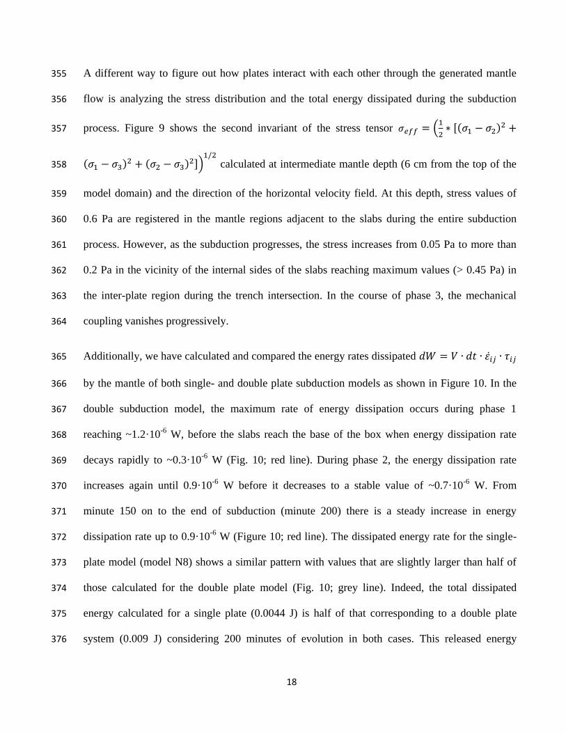
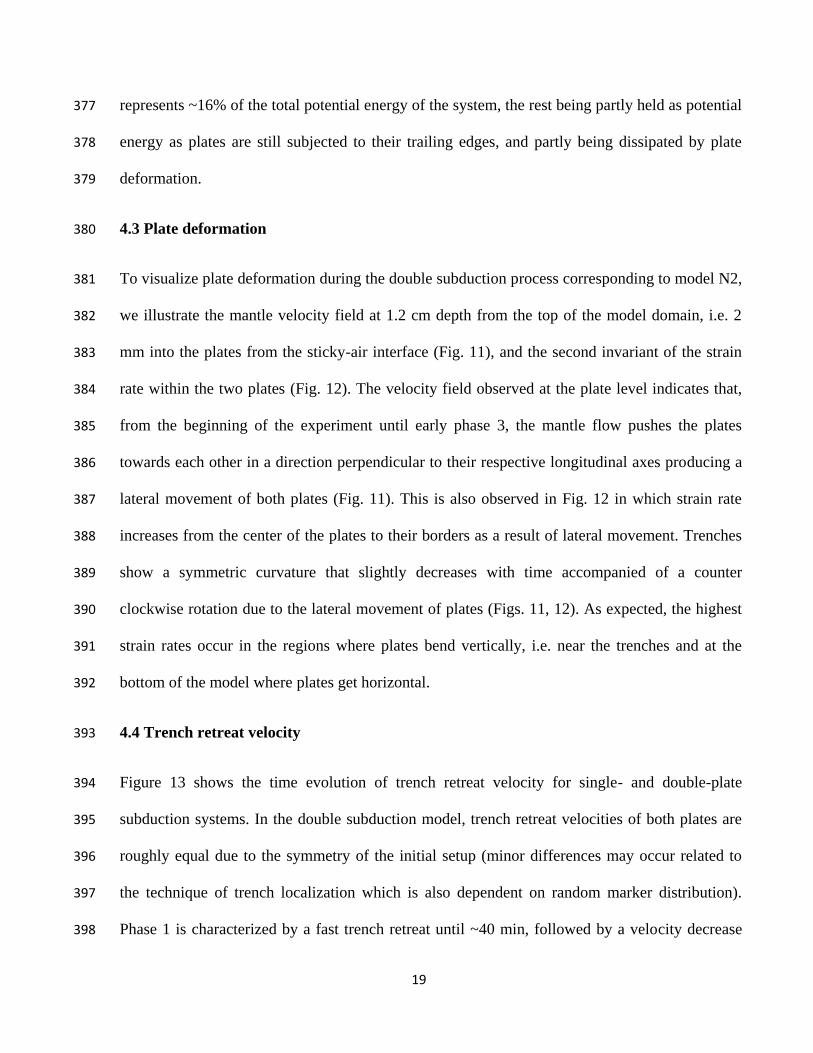
4.2 Stress and energy dissipation 354
18
A different way to figure out how plates interact with each other through the generated mantle 355
flow is analyzing the stress distribution and the total energy dissipated during the subduction 356
process. Figure 9 shows the second invariant of the stress tensor 𝜎𝑒𝑓𝑓 = (1
2∗ [(𝜎1 − 𝜎2)2 +357
(𝜎1 − 𝜎3)2 + (𝜎2 − 𝜎3)2])1/2
calculated at intermediate mantle depth (6 cm from the top of the 358
model domain) and the direction of the horizontal velocity field. At this depth, stress values of 359
0.6 Pa are registered in the mantle regions adjacent to the slabs during the entire subduction 360
process. However, as the subduction progresses, the stress increases from 0.05 Pa to more than 361
0.2 Pa in the vicinity of the internal sides of the slabs reaching maximum values (> 0.45 Pa) in 362
the inter-plate region during the trench intersection. In the course of phase 3, the mechanical 363
coupling vanishes progressively. 364
Additionally, we have calculated and compared the energy rates dissipated 𝑑𝑊 = 𝑉 ∙ 𝑑𝑡 ∙ 𝜀�̇�𝑗 ∙ 𝜏𝑖𝑗 365
by the mantle of both single- and double plate subduction models as shown in Figure 10. In the 366
double subduction model, the maximum rate of energy dissipation occurs during phase 1 367
reaching ~1.2·10-6
W, before the slabs reach the base of the box when energy dissipation rate 368
decays rapidly to ~0.3·10-6
W (Fig. 10; red line). During phase 2, the energy dissipation rate 369
increases again until 0.9·10-6
W before it decreases to a stable value of ~0.7·10-6
W. From 370
minute 150 on to the end of subduction (minute 200) there is a steady increase in energy 371
dissipation rate up to 0.9·10-6
W (Figure 10; red line). The dissipated energy rate for the single-372
plate model (model N8) shows a similar pattern with values that are slightly larger than half of 373
those calculated for the double plate model (Fig. 10; grey line). Indeed, the total dissipated 374
energy calculated for a single plate (0.0044 J) is half of that corresponding to a double plate 375
system (0.009 J) considering 200 minutes of evolution in both cases. This released energy 376
19
represents ~16% of the total potential energy of the system, the rest being partly held as potential 377
energy as plates are still subjected to their trailing edges, and partly being dissipated by plate 378
deformation. 379
4.3 Plate deformation 380
To visualize plate deformation during the double subduction process corresponding to model N2, 381
we illustrate the mantle velocity field at 1.2 cm depth from the top of the model domain, i.e. 2 382
mm into the plates from the sticky-air interface (Fig. 11), and the second invariant of the strain 383
rate within the two plates (Fig. 12). The velocity field observed at the plate level indicates that, 384
from the beginning of the experiment until early phase 3, the mantle flow pushes the plates 385
towards each other in a direction perpendicular to their respective longitudinal axes producing a 386
lateral movement of both plates (Fig. 11). This is also observed in Fig. 12 in which strain rate 387
increases from the center of the plates to their borders as a result of lateral movement. Trenches 388
show a symmetric curvature that slightly decreases with time accompanied of a counter 389
clockwise rotation due to the lateral movement of plates (Figs. 11, 12). As expected, the highest 390
strain rates occur in the regions where plates bend vertically, i.e. near the trenches and at the 391
bottom of the model where plates get horizontal. 392
4.4 Trench retreat velocity 393
Figure 13 shows the time evolution of trench retreat velocity for single- and double-plate 394
subduction systems. In the double subduction model, trench retreat velocities of both plates are 395
roughly equal due to the symmetry of the initial setup (minor differences may occur related to 396
the technique of trench localization which is also dependent on random marker distribution). 397
Phase 1 is characterized by a fast trench retreat until ~40 min, followed by a velocity decrease 398
20
until the tips of the plates reach the base of the model box at around 53 min (Fig. 13). During 399
phase 2, trench retreat velocity increases again reaching a maximum of ~1.6 mm/min followed 400
by a short period of velocity decrease before trenches intersect at around 102 min. Phase 3 is 401
characterized by a progressive increase in retreat velocity reaching maximum values of ~1.9 402
mm/min at the late stage of evolution. The single plate model (model N8) shows similar trench 403
retreat velocity variations during all phases of the subduction process although is slightly faster 404
reaching a maximum velocity of ~2.1 mm/min during phase 1 (Fig. 13). The higher speed 405
computed in the single plate model relative to the double plate model is consistent with the 406
calculated energy dissipation rate, which is slightly higher than half of that for the double plate 407
model (Fig. 10). As the total energy is exactly half, the time over which the energy rate is 408
integrated must be lower and therefore, the velocity faster. 409
410
5 DISCUSSION 411
In the following, numerical results are discussed with respect to the three main objectives 412
introduced earlier, which include 1) testing the effects of rheology and boundary conditions and 413
compare them to laboratory experiments in terms of temporal and structural evolution, 2) 414
investigating and quantifying mantle flow and plate deformation in a double subduction 415
experiment, and 3) comparing the obtained numerical data to natural cases of double subduction. 416
5.1. Comparison of numerical and laboratory experiments 417
Numerically reproducing laboratory experiments is not straightforward. Indeed, other authors 418
already found differences in the sinking and retreating rates and plate morphology when 419
attempting to numerically reproduce laboratory experiments of single-plate subduction [Mériaux 420
21
et al., 2018; Schmeling et al., 2008]. Performing both models simultaneously helps us to control 421
all the parameters affecting the evolution of the system. The agreement between results from 422
numerical and laboratory models is fairly good when considering an intermediate domain size 423
(80 x 80 cm2) with free-slip boundary conditions for the lateral sides and no-slip at the bottom of 424
the numerical model, although the effect of applying different lateral boundary conditions is 425
weak. First-order observations like temporal evolution of subduction, plate and trench 426
geometries, plate deformation and mantle flow are similar in both models (Figs. 2 and 12). 427
However, the two methodologies produce also slight differences. For example, the experimental 428
uncertainties related to the handling process of the laboratory experiments can lead to 429
asymmetries between plates in the initial stages of the evolution of the system or to slight 430
modifications in the rheology of materials. Nevertheless, we found that these factors, which are 431
complex to quantify, produce only second-order differences. 432
Aside these differences related to inaccuracies from the experimental handling, there are 433
others related to simplifications made in the numerical approach. For example, the overall slab 434
deformation as well as the temporal evolution of the subduction process is more accurately 435
reproduced when applying no-slip boundary conditions at the bottom of the model domain (Fig. 436
5). However, the laboratory experiments show that the plates stretch and extend horizontally 437
once lying on the model box floor (Fig. 12), indicating that the analog boundary condition ranges 438
in between those end members (free slip / no slip). An intermediate boundary condition is also 439
expected for the horizon separating the upper from the lower mantle, where an increase in 440
viscosity with a factor of 10 to 100 indicates resistance but does not prohibit viscous drag [e.g., 441
Király et al., 2017; Goes et al., 2017]. 442
22
Furthermore, numerical experiments cannot reproduce simultaneously the large trench curvature 443
and the retreat velocity observed in laboratory experiments, particularly for wide plates, even 444
when varying the rheological parameters (Fig. 6). This points towards potential effects that were 445
not taken into account as the formation of a thin "crystalized" layer at the surface of the syrup, 446
which might generate surface forces not considered in the numerical model [e.g., Mériaux et al., 447
2018]. 448
Concerning double subduction systems with opposite polarity, numerical and analog experiments 449
are in general agreement in terms of overall duration of the subduction process. Furthermore, 450
stresses generated in the inter-plate region in both numerical and analog models, tend to separate 451
the plates from each other (Figs. 9, 11; and Fig. 7 in Peral et al., 2018). However, some 452
discrepancies between the results of the two modeling approaches should be discussed in more 453
detail: Analog experiments show a divergent displacement of the two plates, whereas in 454
numerical experiments the resulting deformation of plates shows a lateral movement that brings 455
the central parts of the plates closer together (Figs. 11, 12). This discrepancy can be explained by 456
the different radii of the toroidal cells generated in both experiments, which seems to be larger in 457
the numerical than in the analog models independently on the size of the modeling domain (Fig. 458
2). Another discrepancy is observed related to trench retreat velocities. Laboratory experiments 459
show retreat velocities increasing until plate intersection and decreasing thereafter [Peral et al., 460
2018], whereas velocities remain roughly constant or even increase towards the end of the 461
subduction process for numerical experiments (Fig. 3, 13). A possible explanation are the 462
different mantle flow patterns and associated evolution of energy dissipation (Fig. 10) that are 463
affected by implemented boundary conditions in numerical models and experimental 464
uncertainties in the analog setup, as well as different rheological properties between analog and 465
23
numerical materials. Concerning the shapes of subducting plates, asymmetric trench curvatures 466
are observed in both numerical and laboratory experiments suggesting that these asymmetries are 467
related to the mantle flow interactions associated with double subduction systems (Fig. 12). A 468
more detailed study of the mantle flow in analog experiments is needed to better understand the 469
observed differences. 470
5.2. Dynamics of double subduction systems 471
Mantle flow in an ideal single-slab subduction system is characterized by a toroidal component 472
that is symmetric relative to the longitudinal axis of the slab. In the case of two adjacent slabs 473
with opposite polarity, the toroidal flows induced by both slabs interact with each other 474
generating different flow patterns in the inter-plate and outer mantle regions. Consequently, the 475
resulting toroidal component of the mantle flow becomes asymmetric relative to the slabs axes 476
(Figs. 7, 11). This asymmetry prevents for applying a half-space model domain as for example in 477
Kiraly et al. [2016], whose setup implies an indefinite repetition of slabs laterally by introducing 478
free-slip side boundaries cutting the opposite polarity slabs. Such boundary conditions are 479
strictly valid for plates exceeding 1000 km width or for tectonic scenarios where the opposed 480
polarity repeats several times. In any case, the resulting flow pattern has important implications 481
for subduction driven by rollback, where the toroidal flow makes up 95–100% of the entire 482
mantle flux [Schellart et al., 2007]. For example, assuming that seismic anisotropy in the upper 483
mantle is related to the lattice preferred orientation of olivine as a result of large-scale mantle 484
flow [e.g., Silver et al., 1996; Long and Becker, 2010] allows detecting complex subduction 485
scenarios and understanding related mantle dynamics [Alpert et al., 2013; Wei et al., 2016]. For 486
double subduction systems similar to the ones presented in this study, the orientation of the 487
24
symmetry axes of the toroidal cells may help interpreting inter-plate coupling and the spatial 488
framework of adjacent trenches (Fig. 7a). 489
Deformation of plates is coupled to the mantle flow and, therefore, affected by mantle flow 490
asymmetry producing lateral movement of the plates and additional deformation of the slabs in 491
double subduction systems (Fig. 12). The deformation experienced by the plates is related to the 492
mantle drag exerted by the net outward flow separating one plate from the other. The strength of 493
this drag decreases with the distance between the slabs, so its effect is maximum during the 494
intersection of the two trenches. Similar behavior has been reported by Király et al. [2016]. The 495
interaction between the flows generated by the two slabs reduces the energy dissipation rate 496
compared to two isolated plates. As a consequence, the trench retreat velocities in a double 497
subduction system are slowed down with respect to a single subduction process. An exception is 498
the end of phase 3 (t >150 min), where plates are sufficiently far from one another and trench 499
retreat is accelerating rather than keeping a constant velocity as in the case of a single plate 500
subduction (Figs. 10, 13). 501
Despite the strong interaction between plates in a double subduction system, the evolution of the 502
trench velocity through time shares some common features with the single subduction system. 503
Obviously, these similarities are stronger during the initial and final stages of the evolution, 504
when the two slabs are distant and the interaction of their induced mantle flows is weaker. For 505
example, as reported elsewhere [Funiciello et al., 2003; Funiciello et al., 2006; Schellart, 2004; 506
Strak and Schellart, 2014], trench velocity increases rapidly at the beginning of the model whilst 507
the slab is sinking and the negative buoyancy increases (Fig. 13; 0 to ~40 min). When the slab 508
reaches the bottom of the domain (40 to 55 min), the trench velocity slows down and accelerates 509
again (from 55 to 75 min) until the steady-state subduction is achieved (75 to 180 min). During 510
25
the steady-state period, the single subduction system shows some minor periodic accelerations 511
and decelerations probably due to changes in the slab angle (Fig. 13). These changes are not so 512
evident in the double subduction system as the interaction between slabs and mantle flow is 513
probably overprinting the slab dip changes. 514
5.3 Relevance for natural prototypes 515
Complex subduction systems formed by several slabs, with reduced dimensions and with 516
advancing or retreating trench migration velocities, can produce changes in the stress, strain rate, 517
and pressure and temperature conditions in the mantle modifying the lattice preferred orientation 518
of olivine crystals and seismic anisotropy as manifested by shear-wave splitting [Faccenda, 519
2014; Faccenda and Capitanio, 2013]. Similarly, the incorporation of sediments and hydrous 520
fluids into the sub-lithospheric mantle during subduction and the rise of the asthenosphere 521
through slab tears or in the backarc extensional basins can result in volcanic activity with a 522
variety of geochemical signatures [e.g., Lustrino et al., 2011; Melchiorre et al., 2017]. 523
As mentioned in the introduction, natural prototypes where double subduction systems with 524
opposite polarity in adjacent segments have been proposed to occur have been identified in 525
Taiwan, New Zealand, the Western Mediterranean and the Alps-Apennine junction, among 526
others. However, extracting conclusions applicable to these natural scenarios is not 527
straightforward as the presented study is based on oversimplified models of double subduction 528
systems. Main limitations are the lack of overriding plates, the assumption of a viscous rheology 529
for the lithosphere and upper mantle, and the dimensions of plates, which at nature scale are 600 530
km wide and 1800 km long separated by a 60-120 km wide transform zone. Despite these 531
26
limitations, we can infer some expected effects derived from the interaction between the plates 532
and the upper mantle in terms of seismic anisotropy and magmatism. 533
One of the regions where these effects are supported by observations is the Western 534
Mediterranean. There, the Alboran-Tethys and the Algerian-Tethys segments retreated in 535
opposite directions inferred from the present distribution and vergence of the metamorphic 536
complexes in the Betic-Rif and the Tell-Kabylies chains [e.g., Casciello et al., 2015; Fernàndez 537
et al., 2019; Vergés and Fernàndez, 2012]. It must be noted that the dimensions of the Ligurian-538
Tethys domain, whose closure gave rise to the present Western Mediterranean, was narrower 539
than the slabs modelled in this study, and the trench intersection occurred before the slabs 540
reached the lower mantle (i.e. during phase 1). Fast polarity directions (FPD) inferred from SKS 541
shear wave splitting onshore show a consistent anisotropy pattern oriented parallel to the Betic-542
Rif orogen [e.g., Díaz et al., 2015; Miller et al., 2013]. Despite the poor coverage of anisotropy 543
data offshore, a regional 3D azimuthally anisotropic model of Europe shows a WSW-ENE 544
alignment of FPD in the Alboran Basin changing to NW-SE in the Algerian Basin at depths of 545
70 – 200 km [Zhu and Tromp, 2013]. At shallower depths however, Pn and Sn tomography 546
shows an almost perpendicular anisotropy pattern for the uppermost mantle with NW-SE 547
oriented FPD in the southern margin of the Alboran Basin varying to NE-SW in the Algerian 548
Basin [Díaz et al., 2013]. These variations in the anisotropy pattern are related to the interaction 549
between the mantle return flows produced by the slabs retreating in opposite directions, the 550
northwest to west displacement of the Alboran-Tethys slab and its tightening, and the absolute 551
motion of the African plate [e.g., Spakman et al., 2018]. 552
The vertical component of mantle flow shows maximum velocities in the back-arc and the inter-553
plate regions being more active during phases 1 and 2 (Figs. 7 and S2-S5). This mantle 554
27
upwelling from the deeper parts of the upper mantle can produce widespread melting by 555
adiabatic decompression with variable composition depending on the water content and the 556
depletion degree of the mantle source, which changes spatially with the retreating of slabs as 557
proposed from recent 3D numerical modeling [e.g., Magni, 2019]. This variable volcanic 558
geochemical signature is observed in the Western Mediterranean magmatic manifestations 559
changing from tholeiitic in the early Oligocene Malaga dikes to calc-alkaline/HK calc-alkaline 560
and alkaline magmas during Late Miocene to Quaternary. The combination of subduction and 561
rifting events operating in the region produced recycling and depletion of mantle rocks making 562
difficult to associate the derived volcanic products with the present-day geodynamic setting [e.g., 563
Carminati et al., 2012; Lustrino and Wilson, 2007; Lustrino et al., 2011; Melchiorre et al., 564
2017]. The limited observations of anisotropy in the offshore regions of the Western 565
Mediterranean, together with the large variety of magmatic compositions, make difficult to favor 566
a unique geodynamic interpretation among those proposed for this region [e.g., Duggen et al., 567
2005; Faccenna et al., 2004; Platt et al., 2013; Spakman and Wortel, 2004; Van Hinsbergen et 568
al., 2014; Vergés and Fernàndez, 2012]. 569
Some of the regions where opposed subduction polarity in adjacent plate segments is observed 570
show a strong trench asymmetry with a tight curvature in one of the ends of the trench (e.g., 571
western Alps, western Betic-Rif, southwest Ryukyu trench). Kiràly et al. [2016] proposed that 572
the stress propagation through the mantle produced by the adjacent retreating slabs contributed to 573
the strong curvature of the Western Alps and the SW-Ryukyu trench. However, according to our 574
results, reproducing the arc tightening observed in the above-mentioned regions would require 575
additional ‘tectonic’ conditions to slow-down or even preventing the slab retreat in one of the 576
plate edges to force the trench curvature. 577
28
The case of New Zealand where the Pacific plate dips to the west beneath the North Island and 578
the Australian plate dips to the east beneath the South Island is more elusive. The interaction 579
between both slabs is doubtful as they are presently separated by the 500 – 600 km long right-580
lateral transform fault, which is the critical distance for stress propagation. The curvature of the 581
Hikurangi Trough could be caused by the fast clockwise rotation of the North Island and the 582
collision of the Chatham Rise microplate with the northern part of the South Island [Wallace et 583
al., 2009; Wallace et al., 2004]. In addition, the comparison with the presented experiments is 584
hindered because subduction of both plates is not synchronous, initiating 25 Ma in the North 585
Island and 10–12 Ma in the South Island [King, 2000; Schellart et al., 2006]. 586
Summarizing, the present work allows for identifying some distinctive features related to 587
subduction systems with opposed polarity in adjacent segments. However, its application to 588
natural prototypes requires a detailed analysis of the tectonic evolution of the study region and 589
the incorporation of a more sophisticated model set-up. 590
591
6. CONCLUDING REMARKS 592
This study presents 3D numerical experiments of subduction systems with opposite polarity of 593
adjacent segments with geometrical and rheological parameters taken from published analog 594
experiments. First, the effects of input parameters such as Eulerian domain size, boundary 595
conditions, and plate geometry and strength were tested and compared to analog results. Second, 596
numerical data was used to better quantify physical processes characterizing the evolution of 597
such double subduction systems and finally for comparison to natural examples. 598
Comparing numerical to analog experiments allows to conclude: 599
29
● The Eulerian domain size has a second-order effect on the overall geometry of plates and 600
the trench retreat velocities during the subduction process. However, elevated velocities 601
along the boundaries of the smallest box setup (30x40 cm2) indicate that there is a critical 602
small domain size beyond which mantle flow is affected. 603
● The choice of lateral boundary conditions (free- vs. no-slip) has a minor effect on the 604
subduction process for the intermediate size experiments. For the bottom boundary, a no-605
slip condition results in plate geometries better comparable to analog experiments, 606
while a free-slip condition moves the bottom-laying plates away from each other. 607
● The trench retreat evolution of subduction systems (single and double) is reproduced very 608
well with rheological and geometrical input data retrieved from analog experiments. 609
However, the trench curvature values obtained from numerical experiments are smaller 610
than the corresponding analogs. This might be due to uncertainties in the measured 611
viscosities from analog experiments or spurious deformation of the plates during 612
handling. 613
● Numerical experiments with thinner and weaker plates can reproduce the trench 614
curvature of analog experiments, but fail in reproducing the trench retreat velocity. This 615
might be due to the crystallization of a fine film on the surface of the syrup. 616
The physical characterization of double subduction systems and its comparison to natural 617
examples gives the following insights: 618
● The mantle flow induced by the subduction of adjacent plates pushes the plates against 619
each other. Simultaneously both downgoing slabs and trenches deform asymmetrically 620
30
and the subduction process evolves slower than the single plate model. During trenches 621
intersection, maximum stresses contribute to further plate deformation. 622
● In the horizontal plane mantle flow forms four toroidal cells with symmetry axes rotating 623
during trench retreat. The flow lines converge towards the front-side of the trenches and 624
diverge from the backside of the trenches. 625
● The upward component of mantle flow is maximum around the sinking slabs before the 626
intersection of trenches and decreases as the slabs retreat concentrating around the edges 627
of the slabs after trenches intersection. 628
● The energy dissipation rate of a plate in a double subduction system is smaller than that 629
of a single subduction. Accordingly, double plate systems exhibit slower trench retreat 630
velocities and a longer duration of the subduction process than a single plate. 631
● The subduction models with opposite polarity in adjacent segments predict complex 632
patterns of seismic anisotropy, magmatic composition and plate deformation associated 633
with the interaction between the sinking slabs and the surrounding mantle. However, its 634
application to natural scenarios needs of a more sophisticated model set-up in terms of 635
plates geometry, rheology and incorporation of overriding plates. 636
637
Acknowledgements 638
We are indebted to two anonymous reviewers, the Associated Editor, and the Editor T. Becker 639
for their valuable comments and suggestions that largely improved the previous version of the 640
manuscript. This work is part of the PhD Thesis of MP developed under the projects SUBTETIS-641
31
CSIC-201830E039, and AGAUR 2017-SGR-847/2017-SGR-1471. We also thank projects 642
AECT-2018-1-0007 and AECT-2018-3-0007 of the Barcelona Supercomputing Center (BSC-643
CNS). JR was supported by the Swiss National Science Foundation (grant number 2-77297-15). 644
SZ thank the funding from AGAUR 2017-SGR-1278, the Agencia Estatal de Investigación 645
project DPI2017-85139-C2-2-R and the European Union project H2020-RISE MATHROCKS 646
GA nº 777778. The grant provided to the Department of Science, Roma Tre University (MIUR‐ 647
ITALY Dipartimenti di Eccellenza, ARTICOLO 1, COMMI 314‐337 LEGGE 232/2016) is 648
gratefully acknowledged by F.F. Datasets for this article are available in 649
http://hdl.handle.net/20.500.11850/364963 (DOI: 10.3929/ethz-b-000364963). 650
651
32
References 652
Alpert, L. A., M.S. Miller, T.W. Becker, and A.A. Allam ( 2013), Structure beneath the Alboran 653
from geodynamic flow models and seismic anisotropy, J. Geophys. Res. Solid Earth, 118, 4265‐ 654
4277. https://doi.org/doi:10.1002/jgrb.50309. 655
Bautista, B. C., M. L. P. Bautista, K. Oike, F. T. Wu, and R. S. Punongbayan (2001), A new 656
insight on the geometry of subducting slabs in Northern Luzon, Philippines, Tectonophysics, 657
339(3-4), 279-310. https://doi.org/10.1016/S0040-1951(01)00120-2. 658
Carminati, E., M. Lustrino, and C. Doglioni (2012), Geodynamic evolution of the central and 659
western Mediterranean: Tectonics vs. igneous petrology constraints, Tectonophysics, 579, 173-660
192. https://doi.org/10.1016/j.tecto.2012.01.026. 661
Casciello, E., M. Fernàndez, J. Vergés, M. Cesarano, and M. Torne (2015), The Alboran domain 662
in the western Mediterranean evolution: The birth of a concept, Bulletin de la Societe 663
Geologique de France, 186(4-5), 371-384. https://doi.org/10.2113/gssgfbull.186.4-5.371. 664
Coltice, N., L. Husson, C. Faccenna, and M. Arnould (2019), What drives tectonic plates?, 665
Science Advances, 5(10). https://doi.org/10.1126/sciadv.aax4295. 666
Di Leo, J. F., A. M. Walker, Z. H. Li, J. Wookey, N. M. Ribe, J. M. Kendall, and A. Tommasi 667
(2014), Development of texture and seismic anisotropy during the onset of subduction, 668
Geochemistry, Geophysics, Geosystems, 15(1), 192-212. https://doi.org/10.1002/2013GC005032. 669
33
Díaz, J., A. Gil, and J. Gallart (2013), Uppermost mantle seismic velocity and anisotropy in the 670
euro-mediterranean region from pn and sn tomography, Geophysical Journal International, 671
192(1), 310-325. https://doi.org/10.1093/gji/ggs016. 672
Díaz, J., J. Gallart, I. Morais, G. Silveira, D. Pedreira, J. A. Pulgar, N. A. Dias, M. Ruiz, and J. 673
M. González-Cortina (2015), From the Bay of Biscay to the High Atlas: Completing the 674
anisotropic characterization of the upper mantle beneath the westernmost Mediterranean region, 675
Tectonophysics, 663. https://doi.org/10.1016/j.tecto.2015.03.007. 676
Duggen, S., K. Hoernle, P. van den Bogaard, and D. Garbe-Schönberg (2005), Post-collisional 677
transition from subduction-to intraplate-type magmatism in the westernmost Mediterranean: 678
Evidence for continental-edge delamination of subcontinental lithosphere, Journal of Petrology, 679
46(6), 1155-1201. https://doi.org/10.1093/petrology/egi013. 680
Faccenda, M. (2014), Mid mantle seismic anisotropy around subduction zones, Physics of the 681
Earth and Planetary Interiors, 227, 1-19. https://doi.org/10.1016/j.pepi.2013.11.015. 682
Faccenda, M., and F.A. Capitanio (2013). Seismic anisotropy around subduction zones: Insights 683
from three-dimensional modeling of upper mantle deformation and SKS splitting calculations. 684
Geochemistry, Geophysics, Geosystems. 14. 243-262. https://doi.org/10.1002/ggge.20055. 685
Faccenna, C., C. Piromallo, A. Crespo-Blanc, L. Jolivet, and F. Rossetti (2004), Lateral slab 686
deformation and the origin of the western Mediterranean arcs, Tectonics, 23(1), TC1012 1011-687
1021. https://doi.org/10.1029/2002TC001488. 688
34
Faccenna, C., A. F. Holt, T. W. Becker, S. Lallemand, and L. H. Royden (2018), Dynamics of 689
the Ryukyu/Izu-Bonin-Marianas double subduction system, Tectonophysics, 746, 229-238. 690
https://doi.org/10.1016/j.tecto.2017.08.011. 691
Fernàndez, M., M. Torne, J. Vergés, E. Casciello, and C. Macchiavelli (2019), Evidence of 692
segmentation in the iberia–africa plate boundary: A jurassic heritage?, Geosciences 693
(Switzerland), 9(8). https://doi.org/10.3390/geosciences9080343. 694
Funiciello, F., C. Faccenna, D. Giardini, and K. Regenauer-Lieb (2003), Dynamics of retreating 695
slabs: 2. Insights from three-dimensional laboratory experiments, Journal of Geophysical 696
Research B: Solid Earth, 108(4), ETG 12-11 - 12-16. https://doi.org/10.1029/2001JB000896. 697
Funiciello, F., M. Moroni, C. Piromallo, C. Faccenna, A. Cenedese, and H. A. Bui (2006), 698
Mapping mantle flow during retreating subduction: Laboratory models analyzed by feature 699
tracking, Journal of Geophysical Research: Solid Earth, 111(3). 700
https://doi.org/10.1029/2005JB003792. 701
Goes, S., R. Agrusta, J. van Hunen, and F. Garel, Subduction-transition zone interaction: A 702
review. Geosphere 13 (3): 644–664. https://doi.org/10.1130/GES01476.1. 703
Gable, C. W., R. J. O'Connell, and B. J. Travis (1991), Convection in three dimensions with 704
surface plates: Generation of toroidal flow, Journal of Geophysical Research: Solid Earth, 705
96(B5), 8391-8405. https://doi.org/10.1029/90JB02743. 706
Gerya (2009), Introduction to numerical geodynamic modelling, 1-345 pp. 707
https://doi.org/10.1017/CBO9780511809101. 708
35
Gerya, and Yuen (2007), Robust characteristics method for modelling multiphase visco-elasto-709
plastic thermo-mechanical problems, Physics of the Earth and Planetary Interiors, 163(1-4), 83-710
105. https://doi.org/10.1016/j.pepi.2007.04.015. 711
Holt, A. F., L. H. Royden, and T. W. Becker (2017), The dynamics of double slab subduction, 712
Geophysical Journal International, 209(1), 250-265. https://doi.org/10.1093/gji/ggw496. 713
King, P. R. (2000), Tectonic reconstructions of New Zealand: 40 Ma to the Present, New 714
Zealand Journal of Geology and Geophysics, 43(4), 611-638. 715
https://doi.org/10.1080/00288306.2000.9514913. 716
Király, Á., F. A. Capitanio, F. Funiciello, and C. Faccenna (2016), Subduction zone interaction: 717
Controls on arcuate belts, Geology, 44(9), 715-718. https://doi.org/10.1130/G37912.1. 718
Király, Á., F. A. Capitanio, F. Funiciello, and C. Faccenna (2017), Subduction induced mantle 719
flow: Length-scales and orientation of the toroidal cell, Earth and Planetary Science Letters, 720
479, 284-297. http://dx.doi.org/10.1016/j.epsl.2017.09.017. 721
Lallemand, Y. Font, H. Bijwaard, and H. Kao (2001), New insights on 3-D plates interaction 722
near Taiwan from tomography and tectonic implications, Tectonophysics, 335(3–4), 229-253. 723
https://doi.org/10.1016/S0040-1951(01)00071-3. 724
Lamb, S. (2011), Cenozoic tectonic evolution of the New Zealand plate-boundary zone: A 725
paleomagnetic perspective, Tectonophysics, 509(3-4), 135-164. 726
https://doi.org/10.1016/j.tecto.2011.06.005. 727
36
Liu, L., and D. R. Stegman (2012), Origin of Columbia River flood basalt controlled by 728
propagating rupture of the Farallon slab, Nature, 482(7385), 386-389. 729
https://doi.org/10.1038/nature10749. 730
Long, M. D. (2016), The Cascadia Paradox: Mantle flow and slab fragmentation in the Cascadia 731
subduction system, Journal of Geodynamics, 102, 151-170. 732
https://doi.org/10.1016/j.jog.2016.09.006. 733
Long, M.D. and T. Becker (2010), Mantle dynamics and seismic anisotropy. Earth and 734
Planetary Science Letters. 297. 341-354. https://doi.org/10.1016/j.epsl.2010.06.036. 735
Lustrino, M., and M. Wilson (2007), The circum-Mediterranean anorogenic Cenozoic igneous 736
province, Earth-Science Reviews, 81(1-2), 1-65. https://doi.org/10.1016/j.earscirev.2006.09.002. 737
Lustrino, M., S. Duggen, and C. L. Rosenberg (2011), The Central-Western Mediterranean: 738
Anomalous igneous activity in an anomalous collisional tectonic setting, Earth-Science Reviews, 739
104(1-3), 1-40. https://doi.org/10.1016/j.earscirev.2010.08.002. 740
Ma, C., Y. Tang, and J. Ying (2019), Magmatism in Subduction Zones and Growth of 741
Continental Crust, Diqiu Kexue - Zhongguo Dizhi Daxue Xuebao/Earth Science - Journal of 742
China University of Geosciences, 44(4), 1128-1142. https://doi.org/10.3799/dqkx.2019.026. 743
Magni, V. (2019), The effects of back-arc spreading on arc magmatism, Earth and Planetary 744
Science Letters, 519, 141-151. https://doi.org/10.1016/j.epsl.2019.05.009. 745
37
Magni, V., M. B. Allen, J. van Hunen, and P. Bouilhol (2017), Continental underplating after 746
slab break-off, Earth and Planetary Science Letters, 474, 59-67. 747
https://doi.org/10.1016/j.epsl.2017.06.017. 748
Melchiorre, M., J. Vergés, M. Fernàndez, M. Coltorti, M. Torne, and E. Casciello (2017), 749
Evidence for mantle heterogeneities in the westernmost Mediterranean from a statistical 750
approach to volcanic petrology, Lithos, 276, 62-74. https://doi.org/10.1016/j.lithos.2016.11.018. 751
Mériaux, C. A., D. A. May, J. Mansour, Z. Chen, and O. Kaluza (2018), Benchmark of three-752
dimensional numerical models of subduction against a laboratory experiment, Physics of the 753
Earth and Planetary Interiors, 283, 110-121. https://doi.org/10.1016/j.pepi.2018.07.009. 754
Miller, M.S., A.A. Allam, T.W. Becker, J. F. Di Leo and J. Wookey (2013), Constraints on the 755
tectonic evolution of the westernmost Mediterranean and northwestern Africa from shear wave 756
splitting analysis, Earth and Planetary Science Letters, Volume 375, Pages 234-243, ISSN 0012-757
821X, https://doi.org/10.1016/j.epsl.2013.05.036. 758
Mishin, Y. A., T. V. Gerya, J. P. Burg, and J. A. D. Connolly (2008), Dynamics of double 759
subduction: Numerical modeling, Physics of the Earth and Planetary Interiors, 171(1-4), 280-760
295. https://doi.org/10.1016/j.pepi.2008.06.012. 761
Panien, M., S. J. H. Buiter, G. Schreurs, and O. Pfiffner (2006), Inversion of a symmetric basin: 762
Insights from a comparison between analogue and numerical experiments, 253-270 pp. 763
https://doi.org/10.1144/GSL.SP. 2006.253.01.13. 764
38
Peral, M., Á. Király, S. Zlotnik, F. Funiciello, M. Fernàndez, C. Faccenna, and J. Vergés (2018), 765
Opposite Subduction Polarity in Adjacent Plate Segments, Tectonics, 37(9), 3285-3302. 766
https://doi.org/10.1029/2017TC004896. 767
Platt, J. P., W. M. Behr, K. Johanesen, and J. R. Williams (2013), The Betic-Rif arc and its 768
orogenic hinterland: A review, in Annual Review of Earth and Planetary Sciences, edited, pp. 769
313-357. https://doi.org/10.1146/annurev-earth-050212-123951. 770
Pusok, A. E. and D. R. Stegman (2019), Formation and stability of same-dip double subduction 771
systems, Journal of Geophysical Research: Solid Earth, 124, 7387-7412. 772
https://doi.org/10.1029/2018JB017027. 773
Schellart, W. (2004), Kinematics of subduction and subduction-induced flow in the upper 774
mantle, Journal of Geophysical Research B: Solid Earth, 109(7), B07401 07401-07419. 775
https://doi.org/10.1029/2004JB002970. 776
Schellart, W., Freeman, J., Stegman, D. et al. (2007), Evolution and diversity of subduction 777
zones controlled by slab width. Nature 446, 308–311. https://doi.org/10.1038/nature05615. 778
Schellart, G. S. Lister, and V. G. Toy (2006), A Late Cretaceous and Cenozoic reconstruction of 779
the Southwest Pacific region: Tectonics controlled by subduction and slab rollback processes, 780
Earth-Science Reviews, 76(3-4), 191-233. https://doi.org/10.1016/j.earscirev.2006.01.002. 781
Schmeling, H., et al. (2008), A benchmark comparison of spontaneous subduction models-782
Towards a free surface, Physics of the Earth and Planetary Interiors, 171(1-4), 198-223. 783
https://doi.org/10.1016/j.pepi.2008.06.028. 784
39
Silver, P. (1996), Seismic anisotropy beneath the continents: Probing the Depths of Geology. 785
Annual Review of Earth and Planetary Sciences 24:1, 385-432. 786
https://doi.org/10.1146/annurev.earth.24.1.385. 787
Spakman, W., and M. Wortel (2004), A Tomographic View on Western Mediterranean 788
Geodynamics, TRANSMED Atlas Mediterr. Reg. Crust Mantle. https://doi.org/10.1007/978-3-789
642-18919-7_2. 790
Spakman, W., M. V. Chertova, A. Van Den Berg, and D. J. J. Van Hinsbergen (2018), Puzzling 791
features of western Mediterranean tectonics explained by slab dragging, Nature Geoscience, 792
11(3), 211-216. https://doi.org/10.1038/s41561-018-0066-z. 793
Strak, V., and W. P. Schellart (2014), Evolution of 3-D subduction-induced mantle flow around 794
lateral slab edges in analogue models of free subduction analysed by stereoscopic particle image 795
velocimetry technique, Earth and Planetary Science Letters, 403, 368-379. 796
https://doi.org/10.1016/j.epsl.2014.07.007. 797
Van Hinsbergen, D. J. J., R. L. M. Vissers, and W. Spakman (2014), Origin and consequences of 798
western Mediterranean subduction, rollback, and slab segmentation, Tectonics, 33(4), 393-419. 799
https://doi.org/10.1002/2013TC003349. 800
Vergés, J., and M. Fernàndez (2012), Tethys-Atlantic interaction along the Iberia-Africa plate 801
boundary: The Betic-Rif orogenic system, Tectonophysics, 579, 144-172. 802
https://doi.org/10.1016/j.tecto.2012.08.032. 803
40
Vignaroli, G., C. Faccenna, L. Jolivet, C. Piromallo, and F. Rossetti (2008), Subduction polarity 804
reversal at the junction between the Western Alps and the Northern Apennines, Italy, 805
Tectonophysics, 450(1-4), 34-50. https://doi.org/10.1016/j.tecto.2008.10.019. 806
Wallace, L. M., S. Ellis, and P. Mann (2009), Collisional model for rapid fore-arc block 807
rotations, arc curvature, and episodic back-arc rifting in subduction settings, Geochemistry, 808
Geophysics, Geosystems, 10(5). https://doi.org/10.1029/2008GC002220. 809
Wallace, L. M., C. Stevens, E. Silver, R. McCaffrey, W. Loratung, S. Hasiata, R. Stanaway, R. 810
Curley, R. Rosa, and J. Taugaloidi (2004), GPS and seismological constraints on active tectonics 811
and arc-continent collision in Papua New Guinea: Implications for mechanics of microplate 812
rotations in a plate boundary zone, Journal of Geophysical Research: Solid Earth, 109(5), 813
B05404 05401-05416. https://doi.org/10.1029/2003JB002481. 814
Wei, W., D. Zhao, J. Xu, et al. (216), Depth variations of P-wave azimuthal anisotropy beneath 815
Mainland China. Scientific Reports 6, 29614. https://doi.org/10.1038/srep29614 816
Zhang, Q., F. Guo, L. Zhao, and Y. Wu (2017), Geodynamics of divergent double subduction: 3-817
D numerical modeling of a Cenozoic example in the Molucca Sea region, Indonesia, Journal of 818
Geophysical Research: Solid Earth, 122(5), 3977-3998. https://doi.org/10.1002/2017JB013991. 819
Zhu, H., and J. Tromp (2013), Mapping tectonic deformation in the crust and upper mantle 820
beneath Europe and the North Atlantic Ocean, Science, 341(6148), 871-875. 821
https://doi.org/10.1126/science.1241335. 822
823
41
Figure captions 824
Figure 1. Model set-up: Scheme of the basic 3D numerical model of double subduction with 825
opposite polarity in adjacent segments with similar material parameters and geometry as in 826
laboratory experiments. Plates are fixed at their trailing edge to enforce rollback. Subduction is 827
initiated by a small slab reaching 3 cm depth. Different configurations varying the size of the box 828
and boundary conditions have been tested. Dimensions shown here correspond to models N2 and 829
N5 (Table 2). 830
Figure 2. Influence of box-size on flow-field: Temporal evolution of numerical double 831
subduction models with 10 cm wide plates and different box sizes (models N1, N2 and N3). 832
Upper row displays the model box size for each column. Intersection stage corresponds to the 833
transition between phase 2 and phase 3. Color arrows indicate the velocity field in the x-z plane 834
(top view) at 6 cm depth from the top of the model domain. Blue and red colors denote the 835
subducted and the buoyant parts of the plate, respectively. Note that models N1 and N2 do not 836
show the mantle flow over the whole box. 837
Figure 3. Influence of box-size on trench retreat: Trench retreat vs time corresponding to 838
numerical models N1 (150 x 150 cm2), N2 (80 x 80 cm
2), N3 (30 x 40 cm
2) and laboratory 839
experiment L1 (150 x 150 cm2). Black and orange dots: trench retreat of plates P1 and P2 of 840
analog experiment L1. Black line: linear regression for both plates of analog experiment. 841
Figure 4. Influence of boundary conditions on trench retreat: Trench retreat vs time 842
corresponding to numerical models N1/N4 (150 x 150 cm2), N2/N5 (80 x 80 cm
2) and N3/N6 843
(30 x 40 cm2) applying different boundary conditions at the lateral walls of the box (x: free-slip; 844
o: no-slip). See Fig. 3 for laboratory results. 845
42
Figure 5. No-slip versus free-slip bottom boundary conditions: Numerical model of double 846
subduction with opposite polarity of 10 cm wide plates during phase 3 with no-slip (a) (model 847
N2) and free-slip (b) (model N7) boundary conditions at the bottom of the box. Color arrows 848
show the mantle flow at 11.9 cm depth from the top of the model domain. 849
Figure 6. Rheology and plate thickness: Single subduction model of 30 cm wide plate carried out 850
in the laboratory and by numerical modeling applying different rheology (𝛾 = 𝜂𝑙/𝜂𝑚) and plate 851
thickness (h). (a) Laboratory experiment L2; (b) Numerical model N10; (c) Numerical model 852
N12; (d) Numerical model N13; (e) Numerical model N15; (f) Numerical model N11. See 853
parameters in Table 2. ‘c’ indicates the trench curvature defined as the ratio between the chord 854
and the sagitta of the circular segment delineated by the trench [see Peral et al., 2018]. 855
Figure 7. Temporal evolution of flow-field illustrating rotation of toroidal cells: Double 856
subduction model N2 shown in top view. Black arrows show the flow direction in the x-z plane 857
at 6 cm depth from the top of the model domain. Background colors indicate the velocity 858
magnitude of the (a) vz, (b) vx and (c) vy components. Stippled straight lines mark the directions 859
of convergent and divergent flows associated with the toroidal cells, which are roughly 860
orthogonal and rotate counterclockwise through time. 861
Figure 8. Velocity field in 3D of double subduction model N2: a) view of the velocity field 862
during intersection of trenches; b) time evolution of the flow direction in a cross-section (plane 863
XY) through the subducting plate 1 (see inset). Background colors indicate the vertical 864
component of the velocity field vy where red and blue correspond to upward and downward 865
movement, respectively. 866
867
43
Figure 9. Effective stress: Top view of the temporal evolution of double subduction model N2. 868
Black arrows show the flow direction in the x-z plane at 6 cm depth from the top of the model 869
domain. White areas denote the location of the slabs. Background colors indicate the effective 870
stress calculated in the mantle at this depth. 871
Figure 10. Energy dissipation rate associated with mantle flow of numerical models N2 (double 872
subduction) and N8 (single subduction). Dashed line would correspond to the energy dissipation 873
rate of two isolated plates. The indicated phases refer to the double subduction model. 874
Figure 11. Plate deformation and flow in the uppermost mantle: Same as figure 7 except flow-875
field plotted at 1.2 cm depth. Dashed rectangles in panel (a) indicate the initial geometry of 876
plates. 877
Figure 12. Strain rate: Temporal evolution of double subduction models with 10 cm wide plates 878
carried out in the laboratory (model L1) and by numerical modeling (model N2), shown in top 879
view. Colors indicate the second invariant of the strain rate (logarithm scale). 880
Figure 13. Trench retreat comparison between single and double subduction: Trench retreat 881
velocity vs time of numerical models N2 (double subduction) and N8 (single subduction). The 882
indicated phases refer to the double subduction model where only one plate is shown due to 883
symmetry of the initial setup. 884
Figure S1. Velocity field on the side walls for models (a) N1, (b) N2 and (c) N3. Note that the 885
size of the model boxes is not on scale with respect to each other. 886
Figure S2. Double subduction model N2 at minute 65 showing the velocity field in the x-z plane 887
at different depths from the top of the model domain. Colors indicate the velocity magnitude of 888
44
the vertical component vy. Red colors indicate upward mantle flow while blue colors indicate 889
downward mantle flow. 890
Figure S3. Double subduction model N2 during intersection (minute 102) showing the velocity 891
field in the x-z plane at different depths from the top of the model domain. Colors indicate the 892
velocity magnitude of the vertical component vy. Red colors indicate upward mantle flow while 893
blue colors indicate downward mantle flow. 894
Figure S4. Double subduction model N2 at minute 168 showing the velocity field in the x-z 895
plane at different depths from the top of the model domain. Colors indicate the velocity 896
magnitude of the vertical component vy. Red colors indicate upward mantle flow while blue 897
colors indicate downward mantle flow. 898
Figure S5. Time evolution of double subduction model N2 showing the velocity field in the 899
inter-plate region. Colors indicate the velocity magnitude of the vertical component vy. Red 900
colors indicate upward mantle flow while blue colors indicate downward mantle flow. 901
902
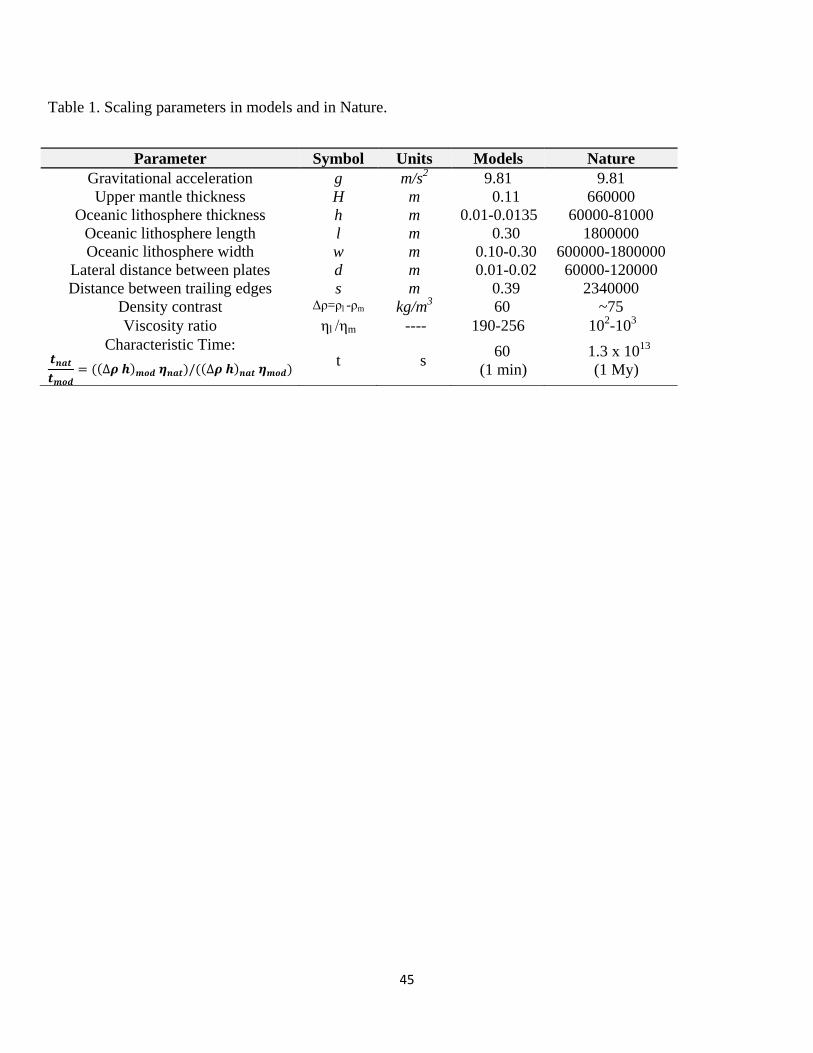
45
Table 1. Scaling parameters in models and in Nature.
Parameter Symbol Units Models Nature
Gravitational acceleration g m/s2 9.81 9.81
Upper mantle thickness H m 0.11 660000
Oceanic lithosphere thickness h m 0.01-0.0135 60000-81000
Oceanic lithosphere length l m 0.30 1800000
Oceanic lithosphere width w m 0.10-0.30 600000-1800000
Lateral distance between plates d m 0.01-0.02 60000-120000
Distance between trailing edges s m 0.39 2340000
Density contrast Δρ=ρl -ρm kg/m3 60 ~75
Viscosity ratio ηl /ηm ---- 190-256 102-10
3
Characteristic Time: 𝒕𝒏𝒂𝒕
𝒕𝒎𝒐𝒅= ((∆𝝆 𝒉)𝒎𝒐𝒅 𝜼𝒏𝒂𝒕)/((∆𝝆 𝒉)𝒏𝒂𝒕 𝜼𝒎𝒐𝒅)
t s 60
(1 min)
1.3 x 10¹³
(1 My)
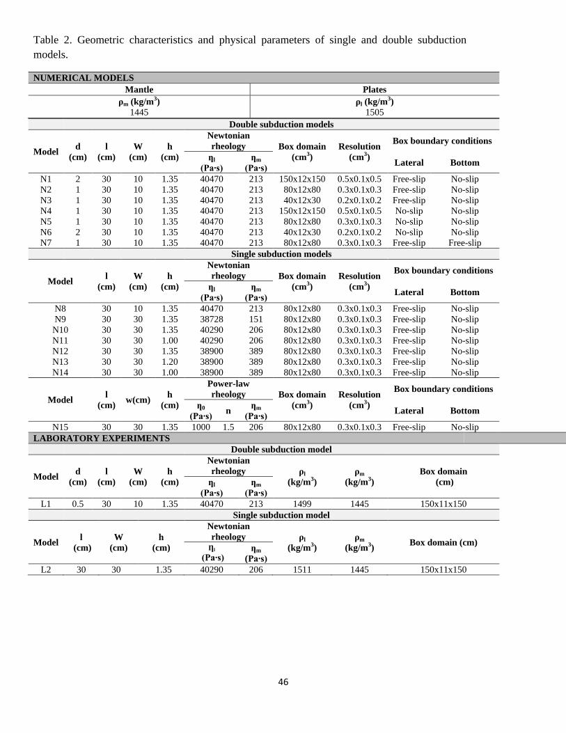
46
Table 2. Geometric characteristics and physical parameters of single and double subduction
models.
NUMERICAL MODELS
Mantle Plates
ρm (kg/m3)
1445
ρl (kg/m3)
1505
Double subduction models
Model d
(cm)
l
(cm)
W
(cm)
h
(cm)
Newtonian
rheology Box domain
(cm3)
Resolution
(cm3)
Box boundary conditions
ƞl
(Pa∙s)
ƞm
(Pa∙s) Lateral Bottom
N1 2 30 10 1.35 40470 213 150x12x150 0.5x0.1x0.5 Free-slip No-slip
N2 1 30 10 1.35 40470 213 80x12x80 0.3x0.1x0.3 Free-slip No-slip
N3 1 30 10 1.35 40470 213 40x12x30 0.2x0.1x0.2 Free-slip No-slip
N4 1 30 10 1.35 40470 213 150x12x150 0.5x0.1x0.5 No-slip No-slip
N5 1 30 10 1.35 40470 213 80x12x80 0.3x0.1x0.3 No-slip No-slip
N6 2 30 10 1.35 40470 213 40x12x30 0.2x0.1x0.2 No-slip No-slip
N7 1 30 10 1.35 40470 213 80x12x80 0.3x0.1x0.3 Free-slip Free-slip
Single subduction models
Model l
(cm)
W
(cm)
h
(cm)
Newtonian
rheology Box domain
(cm3)
Resolution
(cm3)
Box boundary conditions
ƞl
(Pa∙s)
ƞm
(Pa∙s) Lateral Bottom
N8 30 10 1.35 40470 213 80x12x80 0.3x0.1x0.3 Free-slip No-slip
N9 30 30 1.35 38728 151 80x12x80 0.3x0.1x0.3 Free-slip No-slip
N10 30 30 1.35 40290 206 80x12x80 0.3x0.1x0.3 Free-slip No-slip
N11 30 30 1.00 40290 206 80x12x80 0.3x0.1x0.3 Free-slip No-slip
N12 30 30 1.35 38900 389 80x12x80 0.3x0.1x0.3 Free-slip No-slip
N13 30 30 1.20 38900 389 80x12x80 0.3x0.1x0.3 Free-slip No-slip
N14 30 30 1.00 38900 389 80x12x80 0.3x0.1x0.3 Free-slip No-slip
Model l
(cm) w(cm)
h
(cm)
Power-law
rheology Box domain
(cm3)
Resolution
(cm3)
Box boundary conditions
ƞ0
(Pa∙s) n
ƞm
(Pa∙s) Lateral Bottom
N15 30 30 1.35 1000 1.5 206 80x12x80 0.3x0.1x0.3 Free-slip No-slip
LABORATORY EXPERIMENTS
Double subduction model
Model d
(cm)
l
(cm)
W
(cm)
h
(cm)
Newtonian
rheology ρl
(kg/m3)
ρm
(kg/m3)
Box domain
(cm) ƞl
(Pa∙s)
ƞm
(Pa∙s)
L1 0.5 30 10 1.35 40470 213 1499 1445 150x11x150
Single subduction model
Model l
(cm)
W
(cm)
h
(cm)
Newtonian
rheology ρl
(kg/m3)
ρm
(kg/m3)
Box domain (cm) Ƞl
(Pa∙s) ƞm
(Pa∙s)
L2 30 30 1.35 40290 206 1511 1445 150x11x150

Figure1.
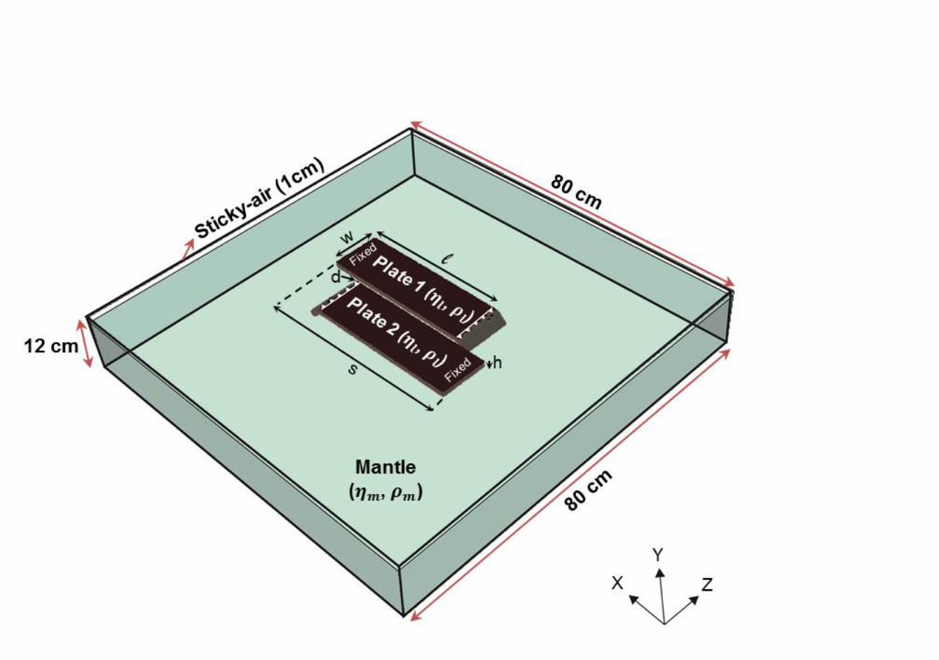

Figure2.
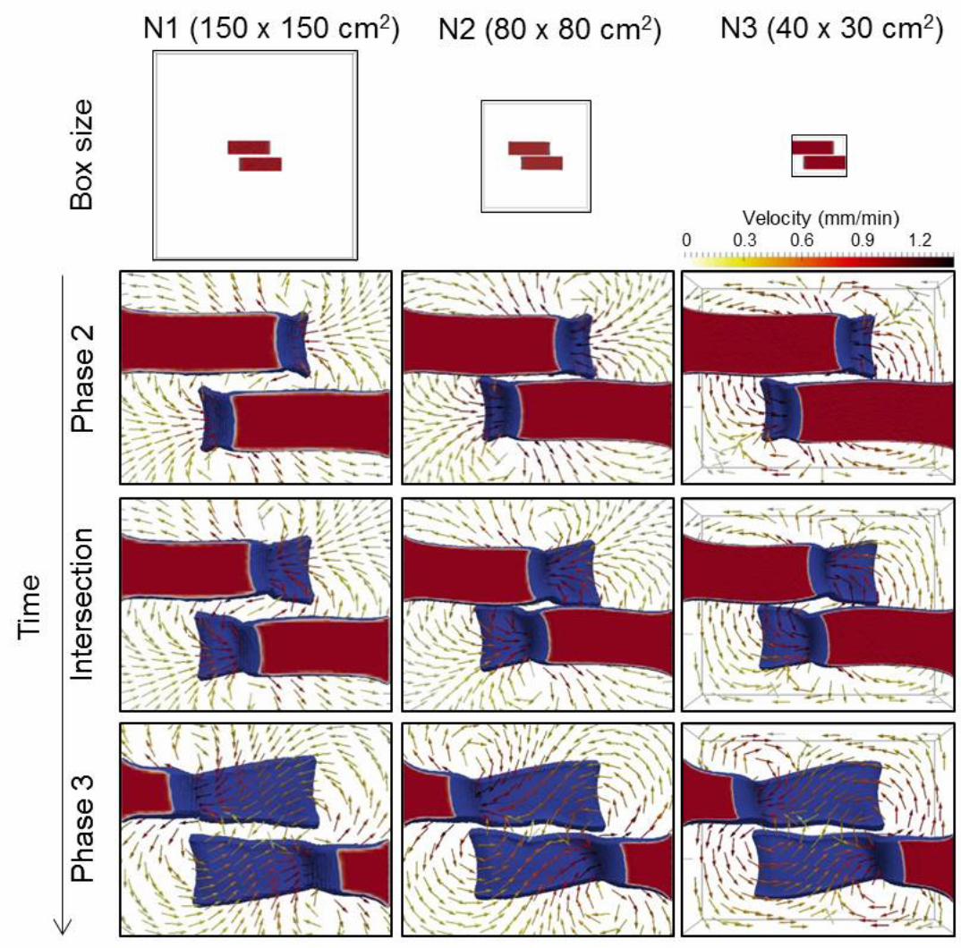

Figure3.
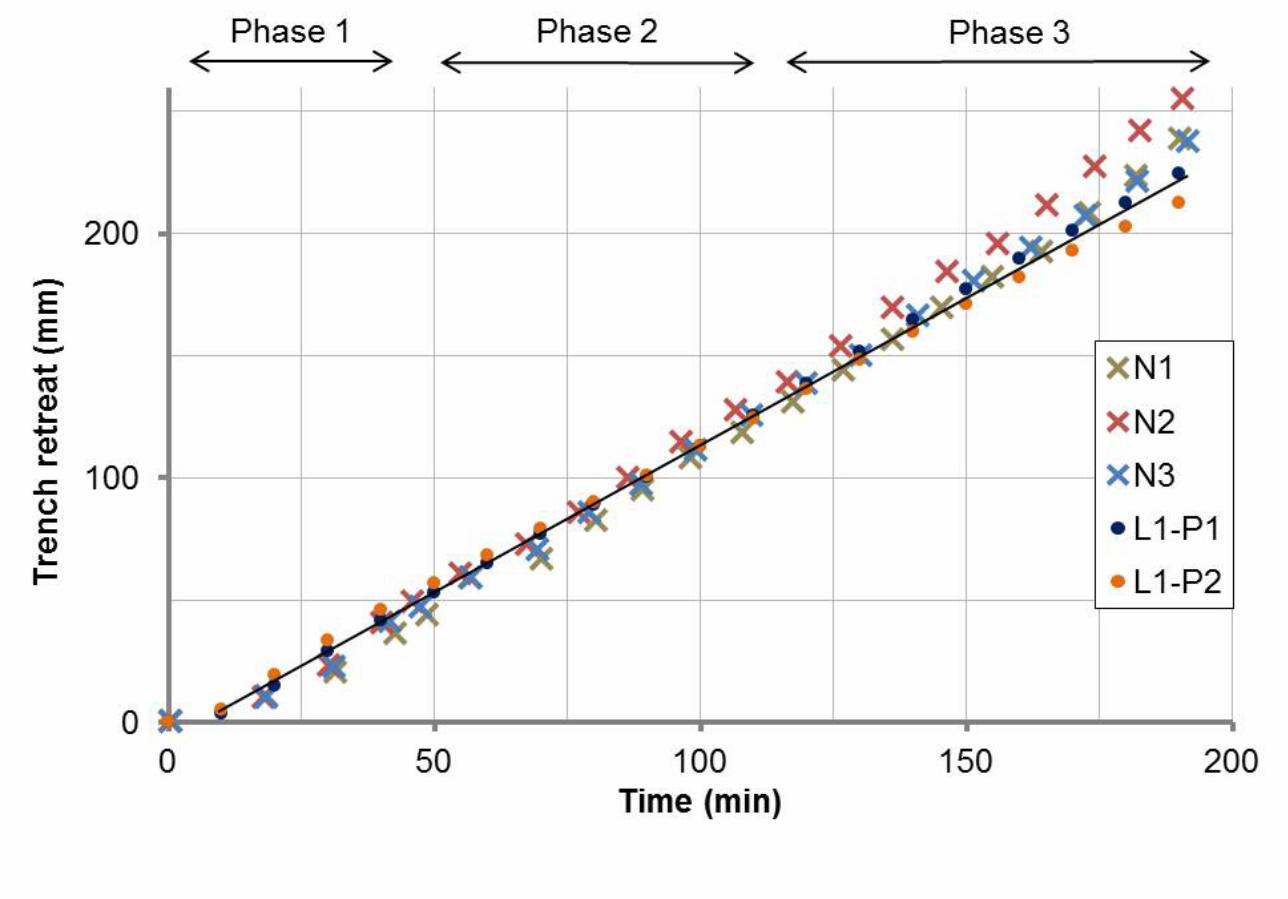

Figure4.
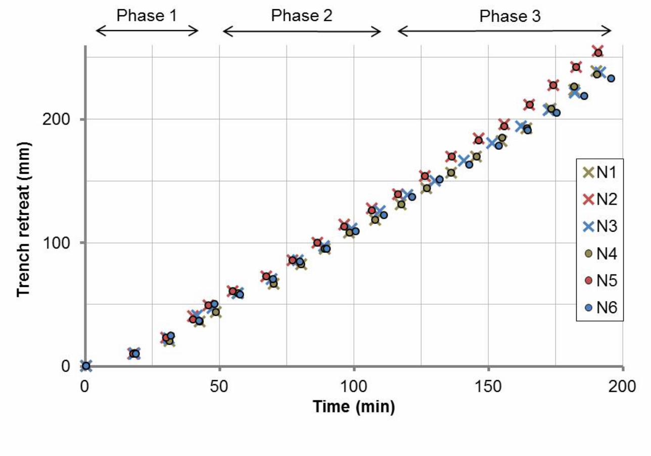

Figure5.
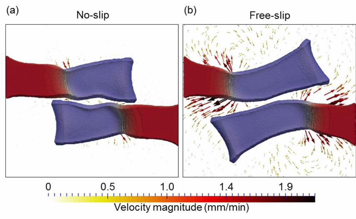

Figure6.
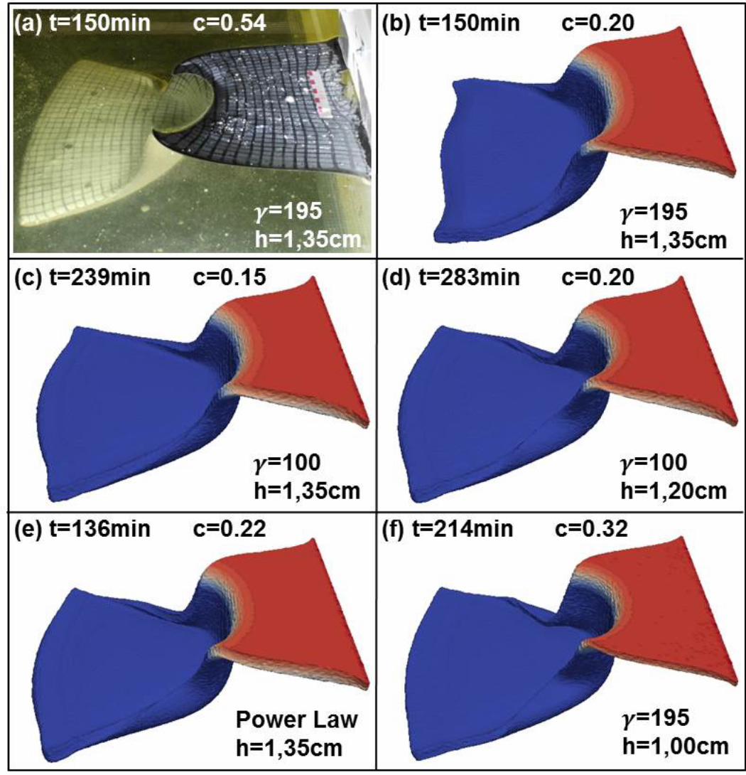

Figure7.
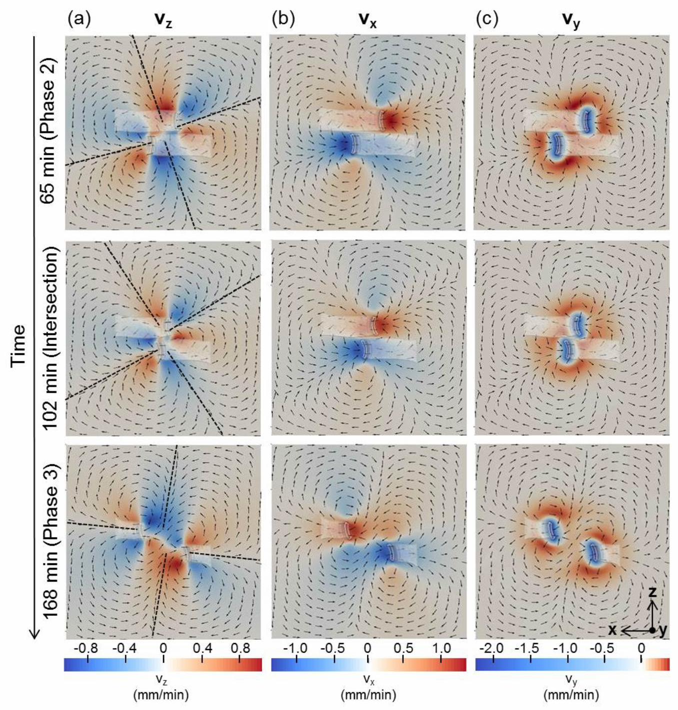

Figure8.
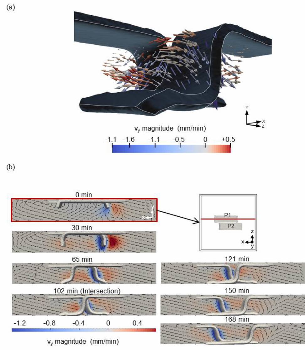

Figure9.
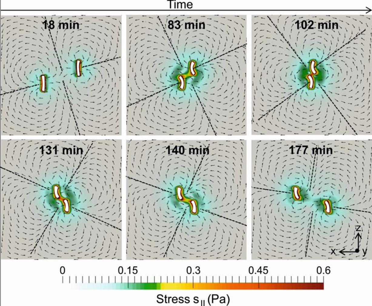

Figure10.
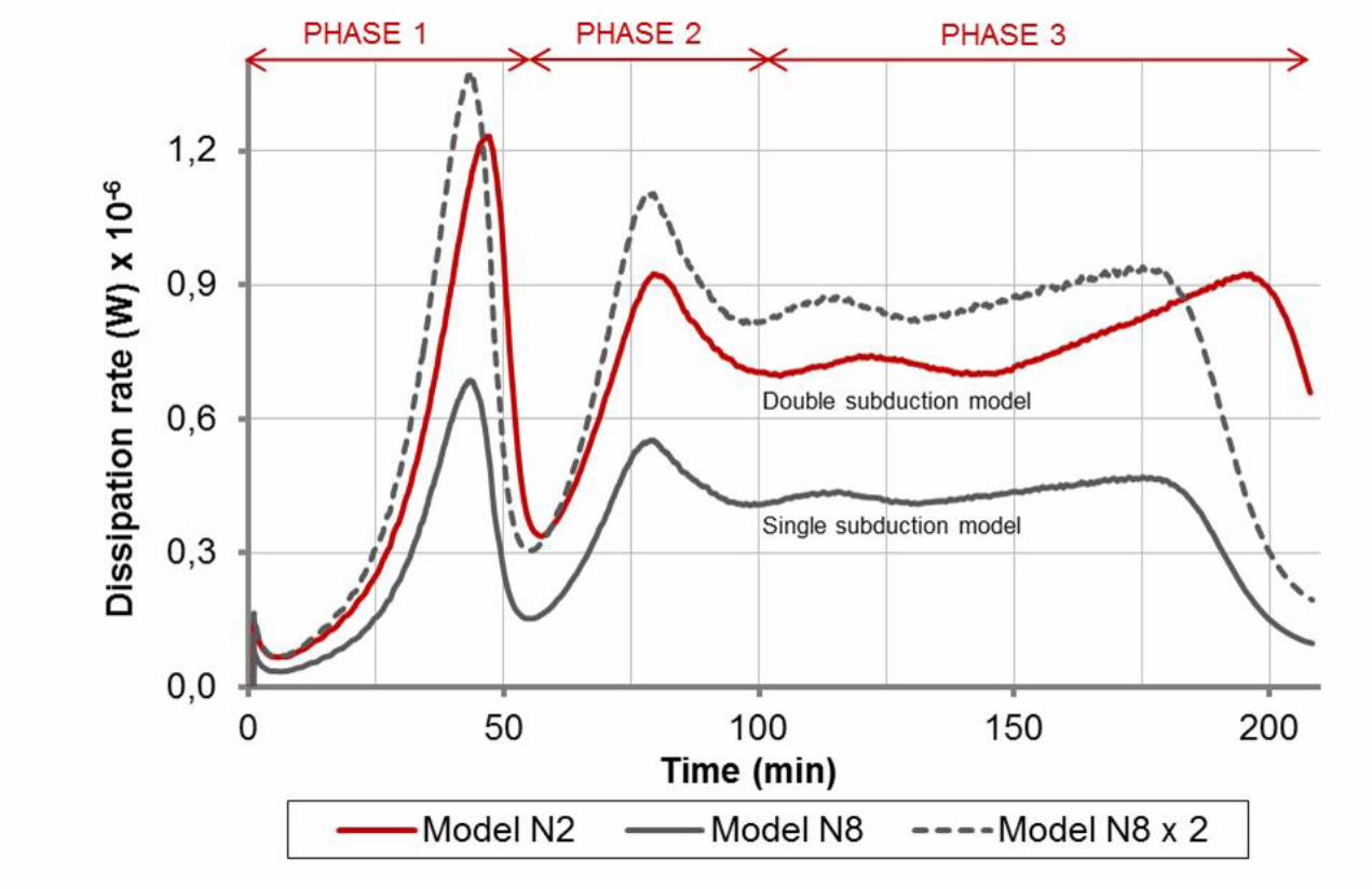

Figure11.
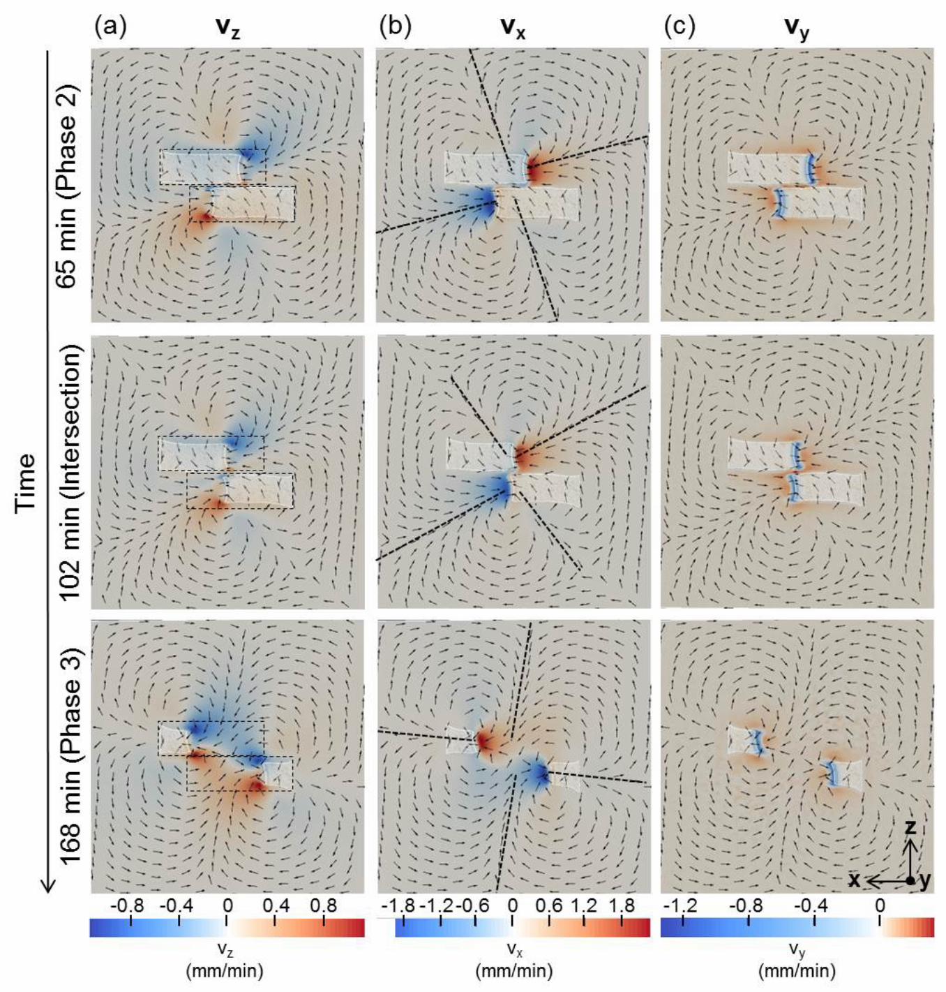

Figure12.
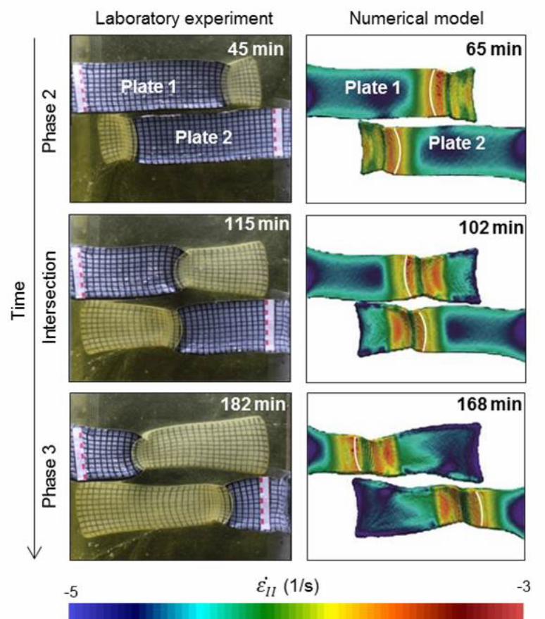

Figure13.
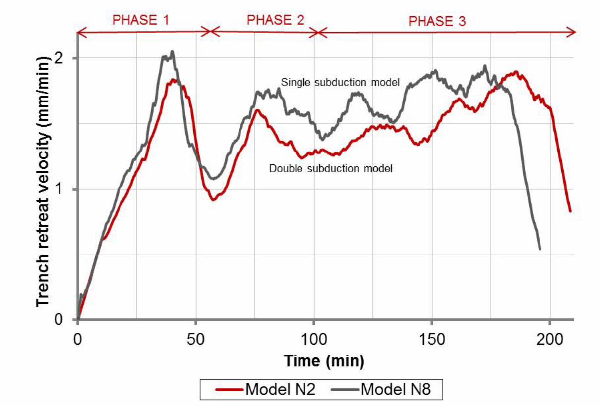

FigureS1.
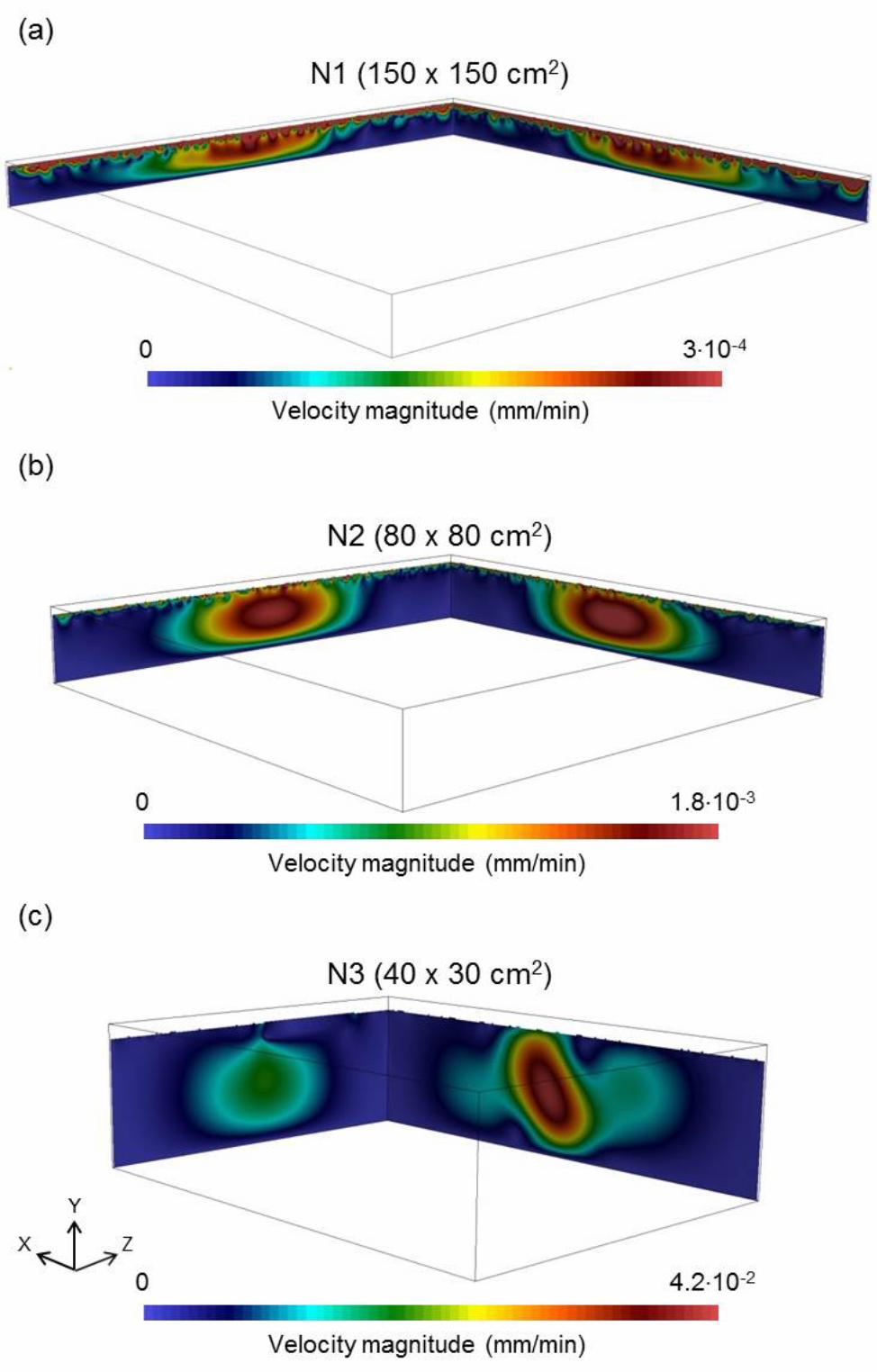

FigureS2.
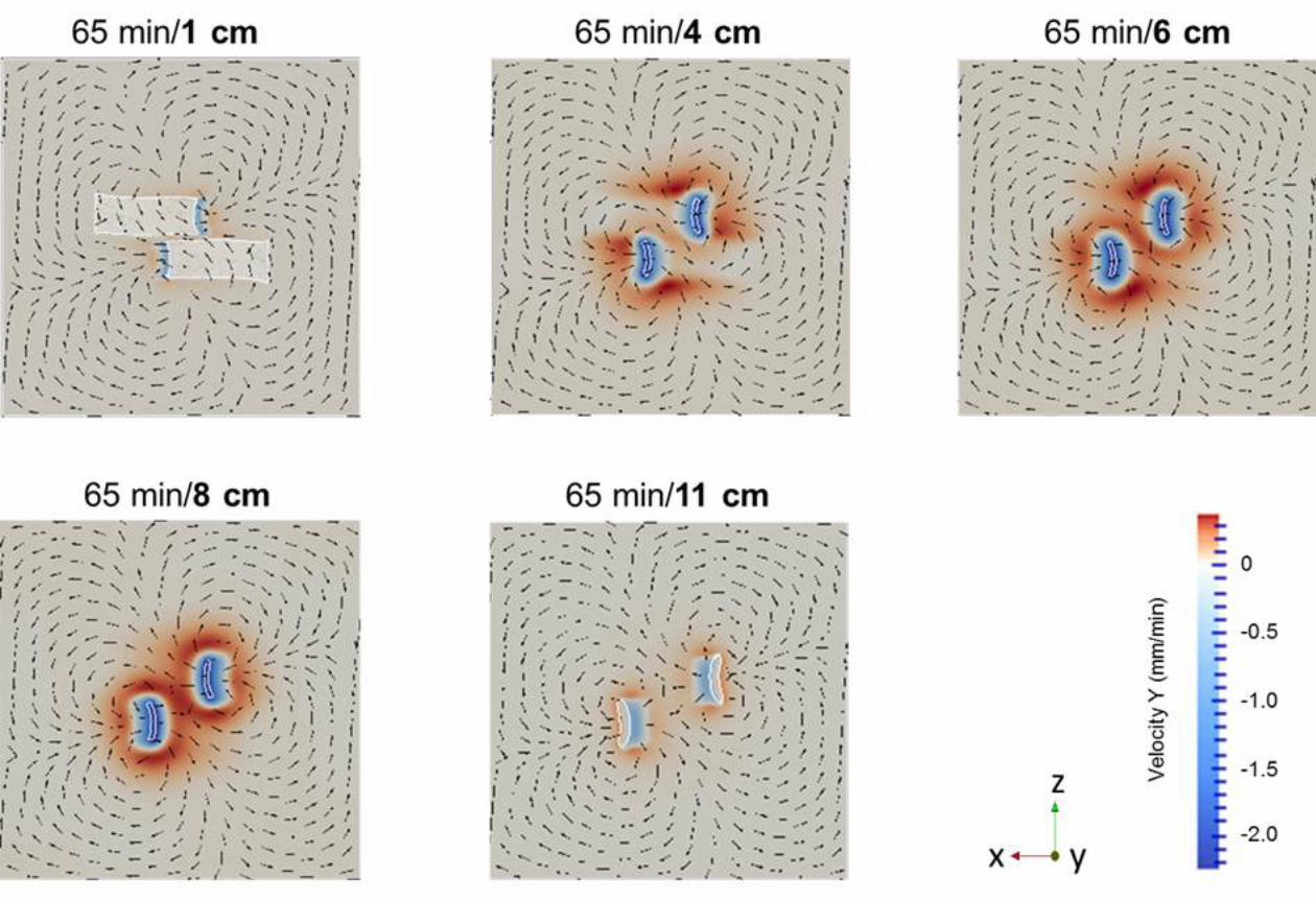

FigureS3.
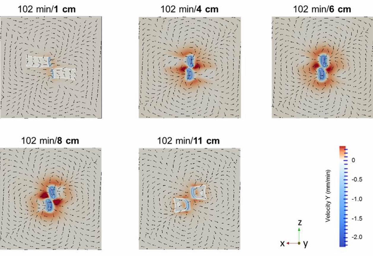

FigureS4.
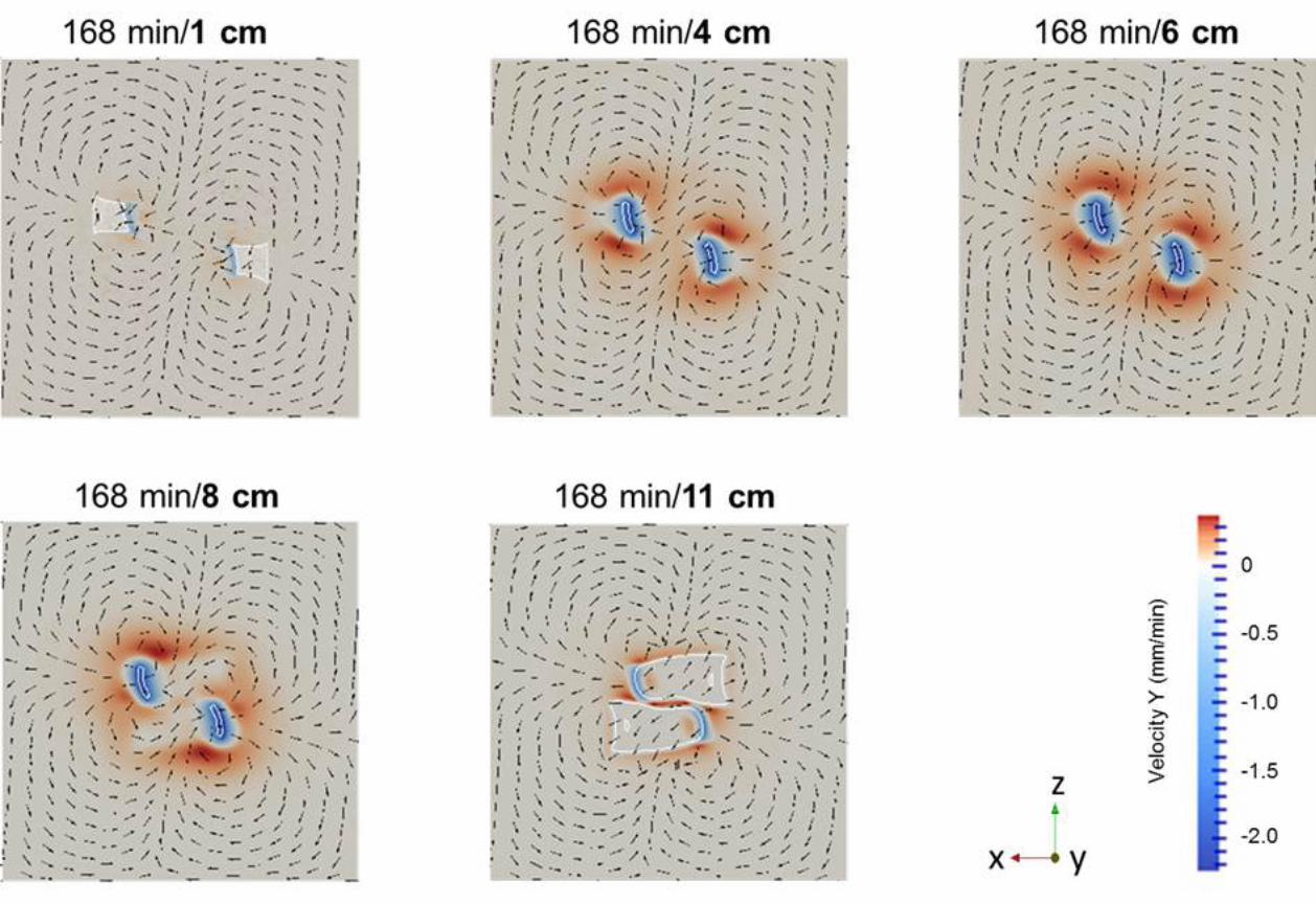

FigureS5.
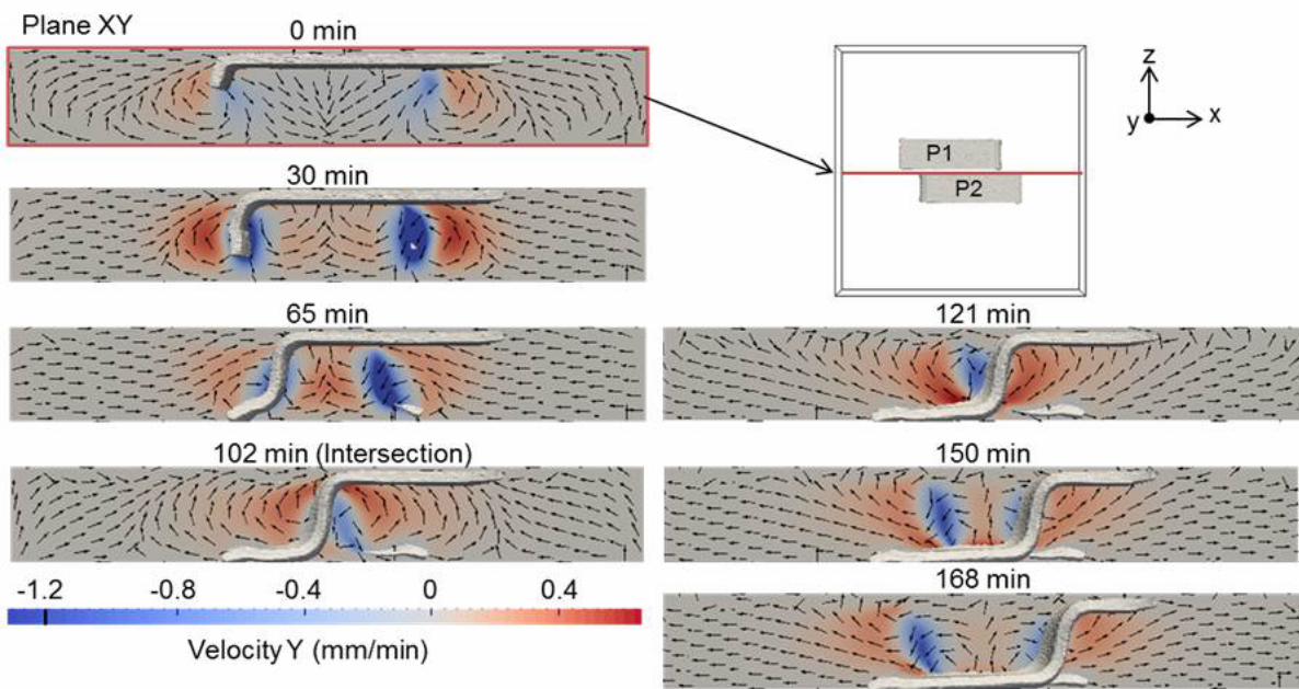


![06 subduction [Kompatibilitätsmodus]](https://img.pdfslide.net/doc/110x75/625a422ab4366065a263fddd/06-subduction-kompatibilittsmodus.jpg)