Embed Size (px)
Citation preview
Persistent link: http://hdl.handle.net/2345/2624
This work is posted on eScholarship@BC,Boston College University Libraries.
Boston College Electronic Thesis or Dissertation, 2008
Copyright is held by the author, with all rights reserved, unless otherwise noted.
The Effects of Using Likert vs. VisualAnalogue Scale Response Options onthe Outcome of a Web-based Survey of4th Through 12th Grade Students: Datafrom a Randomized Experiment
Author: Kevon R. Tucker-Seeley
BBOOSSTTOONN CCOOLL LL EEGGEE LL yynncchh SScchhooooll ooff EEdduuccaatt ii oonn
Department of Educational Research, Measurement, and Evaluation Educational Research, Measurement, and Evaluation Doctoral Program
THE EFFECTS OF USING LIKERT VS. VISUAL ANALOGUE SCALE RESPONSE OPTIONS ON THE OUTCOME OF A WEB-BASED
SURVEY OF 4TH THROUGH 12TH GRADE STUDENTS: DATA FROM A RANDOMIZED EXPERIMENT
Dissertation
by
KK EEVVOONN RR.. TTUUCCKK EERR--SSEEEELL EEYY
submitted in partial fulfillment of the requirements
for the degree of
Doctor of Philosophy
December, 2008

©Copyright by KEVON R. TUCKER-SEELEY 2008

Abstract
THE EFFECTS OF USING LIKERT VS. VISUAL ANALOGUE SCALE RESPONSE
OPTIONS ON THE OUTCOME OF A WEB-BASED SURVEY OF 4TH THROUGH
12TH GRADE STUDENTS: DATA FROM A RANDOMIZED EXPERIMENT
Dissertation by: Kevon R. Tucker-Seeley
Chair: Prof. Michael K. Russell
For more than a half century surveys and questionnaires with Likert-scaled items
have been used extensively by researchers in schools to draw inferences about students;
however, to date there has not been a single study that has examined whether alternative
item response types on a survey might lead to different results than those obtained with
Likert scales in a K-12 setting. This lack of direct comparisons leaves the best method of
framing response options in educational survey research unclear.
In this study, 4th through 12th grade public school students were administered two
versions of the same survey online: one with Likert-scaled response options and the other
with visual analogue-scaled response options. A randomized, fixed-effect, between-
subjects experimental design was implemented to investigate whether the survey with
visual analogue-scaled items yielded results comparable to the survey with Likert-scaled
items based on the following four methods and indices: 1) factor structure; 2) internal
ii
consistency and test-retest reliability; 3) survey summated scores; and 4) main,
interaction, and simple effects.
Results of the first three indices suggested that both the Likert scale and visual
analogue scale produced similar factor structures, were equally reliable, and yielded
summated scores that were not significantly different across all three school levels
(elementary, middle, and high school). Results of the factorial ANOVA suggested that
only the main effect of school level was statistically significant but that there was no
significant interaction between item response type and school level. Results of the post-
survey questionnaires suggested that students at all school levels preferred answering
questions on the survey with the VAS compared to the LS nearly three to one.

iii
Acknowledgments
I would like to thank my dissertation advisor, Dr. Michael Russell for his
thoughtful comments and advice throughout the dissertation process as well as for his
support during my time here at Boston College. I would also like to extend my sincere
gratitude to the other members of my dissertation committee, Dr. Penny Hauser-Cram
and Dr. Laura O’Dwyer, for their invaluable feedback, and expert opinions. They each
contributed in ways that helped me to become a better writer and helped my dissertation
to become something I can be proud of.
I would also like to thank my mom (who tried her best to understand what this
whole “dissertation thing” was all about). To my amazing friends (and second family),
Pam and Michelle, whose laughter, hospitality, and unwavering support has made life
that much sweeter over the years: Thank you. Merci. Gracias!
Last, but certainly not least, I want to especially thank my partner and best friend,
Dr. Reginald Tucker-Seeley, for his unwavering support and for being so patient with me
as I endeavored to stay focused and committed to finishing this dissertation. Words alone
can hardly convey the gratitude I feel for having had him by my side during this entire
process to listen when I needed to vent, to commiserate when things got tough, and to
encourage me just when I needed it most. Reggie: You are the smartest and most
thoughtful person I have ever known and I am a much better person for having known
you. Thank you.

iv
Table of Contents
ABSTRACT ............................................................................................................................ i
ACKNOWLEDGMENTS ........................................................................................................ iii
L IST OF TABLES ............................................................................................................... viii
L IST OF FIGURES ................................................................................................................ x
CHAPTER 1: DEFINING THE PROBLEM ............................................................................. 1
INTRODUCTION .......................................................................................................................................... 1 THE PROBLEM ........................................................................................................................................... 2 RESEARCH PURPOSE ................................................................................................................................. 7
Research Questions ................................................................................................................................ 9 SIGNIFICANCE OF THE STUDY ................................................................................................................. 10 SUMMARY ................................................................................................................................................ 10
CHAPTER 2: L ITERATURE REVIEW ................................................................................. 13
INTRODUCTION ........................................................................................................................................ 13 MEASUREMENT ISSUES IN EDUCATIONAL SURVEY RESEARCH ............................................................. 13
Survey Errors ....................................................................................................................................... 15 Reliability. ....................................................................................................................................... 16
ORDINAL VS . INTERVAL MEASUREMENT................................................................................................ 19 Ordinal Measurement Scale ................................................................................................................. 19 Interval Measurement Scale ................................................................................................................. 20
Treating ordinal data as interval. ................................................................................................... 20 MEASURING SURVEY RESPONSES ........................................................................................................... 22
The Likert Scale ................................................................................................................................... 22 Response issues with LS items......................................................................................................... 24
The Visual Analogue Scale .................................................................................................................. 26 Likert Scales: Ordinal or Interval? ....................................................................................................... 29 Visual Analog Scales: Ordinal or Interval? ......................................................................................... 31
CHILDREN AND SURVEYS ........................................................................................................................ 33 Cognitive Development ....................................................................................................................... 33
Piaget’s concrete operations vs. formal operations. ....................................................................... 33 Children’s Ability to Self-Report......................................................................................................... 35
CHILDREN AND L IKERT SCALES VS. VISUAL ANALOGUE SCALES ......................................................... 37 VAS and Children ................................................................................................................................ 38
VAS and children’s ability to understand measurement and scale. ................................................ 40 VAS and K-12 educational research. .............................................................................................. 42
WEB-BASED SURVEYS ............................................................................................................................. 45 VAS and Web-based research ............................................................................................................. 45
Web-based vs. paper-based VAS surveys. ....................................................................................... 47
v
Mode Effects and Sensitive Questions................................................................................................. 48 SUMMARY ................................................................................................................................................ 49
CHAPTER 3: METHODS .................................................................................................... 51
INTRODUCTION ........................................................................................................................................ 51 RESEARCH DESIGN .................................................................................................................................. 51
Justification for the Experimental Design ............................................................................................ 54 SAMPLING METHOD ................................................................................................................................ 54
Teacher Recruitment ............................................................................................................................ 54 Student Participation ............................................................................................................................ 55
PARTICIPANTS .......................................................................................................................................... 56 Inclusion Criteria ................................................................................................................................. 56 Exclusion Criteria ................................................................................................................................ 56 Random Assignment ............................................................................................................................ 58 Effect Size, Power, and Sample Size ................................................................................................... 59
INSTRUMENTATION .................................................................................................................................. 60 Identification with School Survey ....................................................................................................... 61
Reported survey reliability. ............................................................................................................. 62 Criteria for selection of instrument. ................................................................................................ 62
Survey Modifications ........................................................................................................................... 63 Survey reading level. ....................................................................................................................... 64 Web-based survey design features. ................................................................................................. 65 Supplemental post-survey questionnaire. ........................................................................................ 65 Student demographic questionnaire. ............................................................................................... 66
Scoring Criteria .................................................................................................................................... 66 Scoring the Likert scale version. ..................................................................................................... 66 Scoring the VAS version. ................................................................................................................. 67
RESEARCH QUESTIONS ............................................................................................................................ 68 STATISTICAL ANALYSES .......................................................................................................................... 68
Data Analysis ....................................................................................................................................... 68 Index 1: Factor Structure ..................................................................................................................... 69
Principal components analysis. ...................................................................................................... 69 Index 2: Reliability .............................................................................................................................. 75
Cronbach’s alpha. ........................................................................................................................... 77 Test-retest reliability. ...................................................................................................................... 77
Index 3: Summated Mean Scale Scores ............................................................................................... 78 Index 4: Simple-, Main-, and Interaction Effects ................................................................................ 78
Factorial ANOVA. ........................................................................................................................... 80 Steps taken to conduct the ANOVA. ................................................................................................ 80
Criterion for Rejecting H0 .................................................................................................................... 81 POSSIBLE THREATS TO VALIDITY ........................................................................................................... 82
Internal Validity Issues ........................................................................................................................ 82 External Validity Issues ....................................................................................................................... 83
CHAPTER 4: RESULTS ...................................................................................................... 84
INTRODUCTION ........................................................................................................................................ 84 SAMPLE .................................................................................................................................................... 84
Categorical Variables ........................................................................................................................... 86 Experimental Conditions ..................................................................................................................... 87
FACTOR STRUCTURE ............................................................................................................................... 88 Research question #1 .......................................................................................................................... 88
vi
Principal Components Analysis ........................................................................................................... 88 Scree Test............................................................................................................................................. 89 Component Loadings Assessment ....................................................................................................... 89 Parallel Analysis Procedure ................................................................................................................. 92 Conclusion ........................................................................................................................................... 96
RELIABILITY COEFFICIENT ..................................................................................................................... 97 Research question #2 .......................................................................................................................... 97 Internal Consistency Reliability ........................................................................................................... 97
Full sample...................................................................................................................................... 97 School-level samples. ...................................................................................................................... 98
Coefficient of Stability ......................................................................................................................... 99 Conclusion ........................................................................................................................................... 99
SUMMATED SCORES: LS VS. VAS ........................................................................................................ 100 Research question #3 ........................................................................................................................ 100 Paired-Samples t Test ........................................................................................................................ 101 Conclusion ......................................................................................................................................... 102
SUMMATED SCORES: SCHOOL -LEVEL COMPARISONS ........................................................................ 102 Research question #4 ........................................................................................................................ 102 School-Level Summated Score Results ............................................................................................. 102 Conclusion ......................................................................................................................................... 103
FACTORIAL ANOVA ............................................................................................................................. 104 Research question #5 ........................................................................................................................ 104 Main Effects....................................................................................................................................... 104 Interaction .......................................................................................................................................... 106 Simple Effects .................................................................................................................................... 108 Conclusion ......................................................................................................................................... 109
POST-SURVEY QUESTIONNAIRE ............................................................................................................ 110 Dichotomous Item Results ................................................................................................................. 110 Qualitative Item Results ..................................................................................................................... 112
Likert scale responses. .................................................................................................................. 113 Visual analogue scale responses. .................................................................................................. 115
Comparison of LS to VAS by School-Level ..................................................................................... 116 Upper Elementary (grades 4-6). ................................................................................................... 117 Middle (grades 7-9). ..................................................................................................................... 117 High School (grades 10-12). ......................................................................................................... 118
SUMMARY .............................................................................................................................................. 119
CHAPTER 5: DISCUSSION AND CONCLUSION ................................................................ 121
OVERVIEW OF FINDINGS ....................................................................................................................... 121 DISCUSSION ............................................................................................................................................ 122
Consistency of Findings ..................................................................................................................... 122 Explaining the Differences in Scores Between School Levels .......................................................... 123 Explaining the Differences in Item Response-Type Preference ........................................................ 124
Piaget’s stages of development. .................................................................................................... 125 The “digital generation”: Today’s media-savvy students. ............................................................ 126
Student Motivation Effects ................................................................................................................ 127 Fatigue. ......................................................................................................................................... 128 Attrition. ........................................................................................................................................ 129 Item nonresponse. ......................................................................................................................... 129
Summary ............................................................................................................................................ 130 STRENGTHS AND L IMITATIONS OF THE STUDY .................................................................................... 131
Strengths ............................................................................................................................................ 131

vii
Limitations ......................................................................................................................................... 131 IMPLICATIONS OF THE STUDY ............................................................................................................... 134 SUGGESTIONS FOR FUTURE RESEARCH ................................................................................................ 135 FINAL CONCLUSIONS ............................................................................................................................. 137
REFERENCES ................................................................................................................... 138
APPENDIX A .................................................................................................................... 150
THE “I DENTIFICATION WITH SCHOOL ” SURVEY (LIKERT SCALE VERSION) .......................................... 150
APPENDIX B .................................................................................................................... 151
THE “I DENTIFICATION WITH SCHOOL ” SURVEY (VAS VERSION) ......................................................... 151
APPENDIX C .................................................................................................................... 152
POST-SURVEY 1: “ STUDENT OPINION QUESTIONNAIRE” .................................................................... 152
APPENDIX D .................................................................................................................... 153
POST-SURVEY 2: “ STUDENT DEMOGRAPHIC QUESTIONNAIRE” .......................................................... 153
APPENDIX E .................................................................................................................... 154
STUDY ADVERTISEMENT FOR TEACHER LISTSERV .......................................................................... 154
APPENDIX F .................................................................................................................... 155
SCREEN SHOT : IDENTIFICATION WITH SCHOOL SURVEY STUDENT ASSENT FORM ............................ 155
APPENDIX G .................................................................................................................... 156
SCREEN SHOT : IDENTIFICATION WITH SCHOOL SURVEY “W ELCOME ” AND “T HANK YOU ” M ESSAGE ................................................................................................................................................................ 156
APPENDIX H .................................................................................................................... 157
SCREEN SHOTS: IDENTIFICATION WITH SCHOOL SURVEY LS “PRACTICE ITEM ” INSTRUCTIONS AND EXAMPLE ............................................................................................................................................... 157
APPENDIX I ..................................................................................................................... 158
SCREEN SHOTS: IDENTIFICATION WITH SCHOOL SURVEY VAS “PRACTICE ITEM ” INSTRUCTIONS AND EXAMPLE ............................................................................................................................................... 158
APPENDIX J ..................................................................................................................... 159
SCREEN SHOTS: IDENTIFICATION WITH SCHOOL SURVEY LS AND VAS ITEM EXAMPLES ................. 159
APPENDIX K .................................................................................................................... 160
PARALLEL ANALYSIS SPSS SYNTAX .................................................................................................... 160

viii
L IST OF TABLES
Table 3-1: Randomized Treatment Conditions ……………………………………..
53
Table 3-2: Main Effects, Interaction, and Degrees of Freedom Summary Table …..
82
Table 4-1: Sample demographic characteristics …………………………................
85
Table 4-2: Grouping Variables by Grade and Age …………………………………
87
Table 4-3: Comparison of component loadings across one vs. two extracted components for the initial solution of the LS and VAS versions of the survey ……..
90
Table 4-4: Identification with School Survey Cronbach’s Alpha Reliability and Descriptive Statistics: LS vs. VAS (full sample) …………………………………...
98
Table 4-5: Identification with School Survey Cronbach’s Alpha Reliability and Descriptive Statistics: LS vs. VAS (by School-Level) ……………………………..
98
Table 4-6: Survey Summated Score Descriptive Statistics: LS vs. VAS (full sample) ………………………………………………………………………………
100
Table 4-7: Survey Item Descriptive Statistics: LS vs. VAS (full sample) ………...
101
Table 4-8: Paired-Samples t Test of LS-VAS Summated Scores (full sample) …...
101
Table 4-9: Paired-Samples t Test of LS-VAS Summated Scores (by School-Level)
103
Table 4-10: Two-way ANOVA Summary Table …………………..………….....…
105
Table 4-11: Post Hoc Tests for Multiple Comparisons of School Level …………...
108
Table 4-12: Cell Means and t-Values for Simple Effects of Item Response Type by School Level ………………………………………………………………………...
109
Table 4-13: Post-Survey Student Opinion Questionnaire Item Response Descriptives ………………………………………………………………………….
112
Table 4-14: Post-Survey Demographic Questionnaire Supplementary Item Response Descriptives ……………………………………………………...……….
112

ix
Table 4-15: LS Post-Survey Questionnaire Open-Response Themes and Student Responses ……………………………………………………………………………
114
Table 4-16: VAS Post-Survey Questionnaire Open-Response Themes and Student Responses ...………………………………………………………………………….
116
Table 4-17: Percent of Negative and Positive Responses Toward the LS and VAS by School-Level ……………………………………………………………………..
117
x
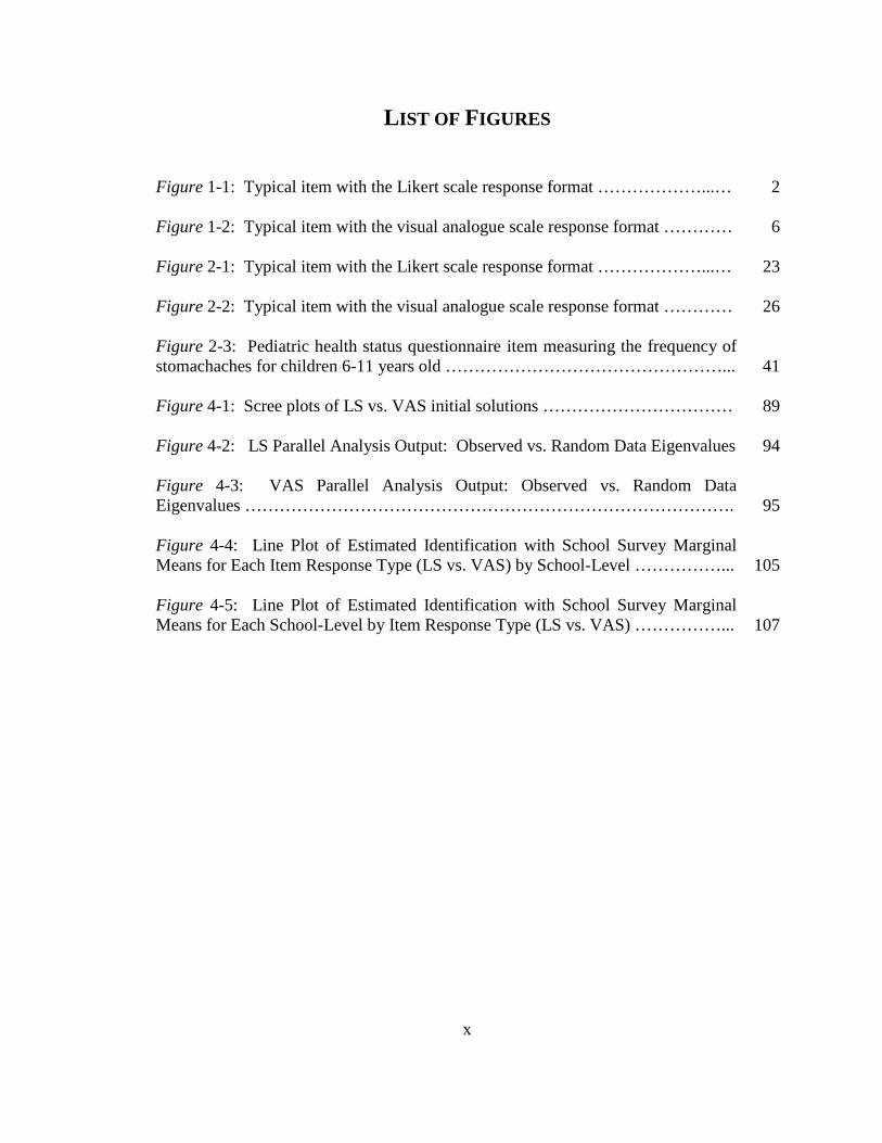
L IST OF FIGURES
Figure 1-1: Typical item with the Likert scale response format ………………...…
2
Figure 1-2: Typical item with the visual analogue scale response format …………
6
Figure 2-1: Typical item with the Likert scale response format ………………...…
23
Figure 2-2: Typical item with the visual analogue scale response format …………
26
Figure 2-3: Pediatric health status questionnaire item measuring the frequency of stomachaches for children 6-11 years old …………………………………………...
41
Figure 4-1: Scree plots of LS vs. VAS initial solutions ……………………………
89
Figure 4-2: LS Parallel Analysis Output: Observed vs. Random Data Eigenvalues
94
Figure 4-3: VAS Parallel Analysis Output: Observed vs. Random Data Eigenvalues ………………………………………………………………………….
95
Figure 4-4: Line Plot of Estimated Identification with School Survey Marginal Means for Each Item Response Type (LS vs. VAS) by School-Level ……………...
105
Figure 4-5: Line Plot of Estimated Identification with School Survey Marginal Means for Each School-Level by Item Response Type (LS vs. VAS) ……………...
107

1
Chapter 1: Defining the Problem
Introduction
For more than a half century surveys with Likert scale (LS) response options have
been used extensively in schools to draw inferences about students. To date, however,
educational researchers have not examined whether a different scale—such as a scale that
employs a continuous response format—would have a similar effect on students’
responses or lead to different results than those obtained from a LS survey in a K-12
setting. This lack of direct comparisons between the LS and other scales leaves the best
method for framing response options in K-12 educational survey research unclear.
Originally proposed by Rensis Likert (1932) as a summated scale1 for the
measurement of respondents’ attitudes, the LS format generally consists of an item
prompt or statement about the attitude being measured (e.g., I enjoy reading mystery
novels) followed by a limited or discrete set of responses designed to capture a
respondent’s personal opinion about (or attitude toward) the item prompt. Typically, the
LS has four to seven response options, each consisting of a single word or short phrase
that differs by varying degrees ranging from one negative extreme to its polar opposite
positive extreme (e.g. from strongly disagree to strongly agree or not at all likely to
highly likely). Respondents are instructed to choose only one response option from those
1 “A scale or index made up of several items measuring the same variable. The responses are given numbers in such a way that responses can be added up [or summated]” (Vogt, 1999, p. 284).
2
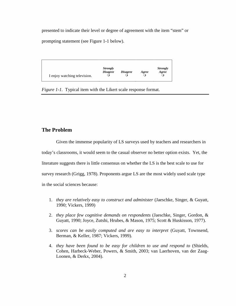
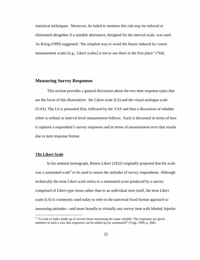
presented to indicate their level or degree of agreement with the item “stem” or
prompting statement (see Figure 1-1 below).
Strongly Disagree Disagree Agree
Strongly Agree
I enjoy watching television. � � � �
Figure 1-1. Typical item with the Likert scale response format.
The Problem
Given the immense popularity of LS surveys used by teachers and researchers in
today’s classrooms, it would seem to the casual observer no better option exists. Yet, the
literature suggests there is little consensus on whether the LS is the best scale to use for
survey research (Grigg, 1978). Proponents argue LS are the most widely used scale type
in the social sciences because:
1. they are relatively easy to construct and administer (Jaeschke, Singer, & Guyatt, 1990; Vickers, 1999)
2. they place few cognitive demands on respondents (Jaeschke, Singer, Gordon, & Guyatt, 1990; Joyce, Zutshi, Hrubes, & Mason, 1975; Scott & Huskisson, 1977).
3. scores can be easily computed and are easy to interpret (Guyatt, Townsend, Berman, & Keller, 1987; Vickers, 1999).
4. they have been found to be easy for children to use and respond to (Shields, Cohen, Harbeck-Weber, Powers, & Smith, 2003; van Laerhoven, van der Zaag-Loonen, & Derkx, 2004).

3
5. they tend to have high reliabilities (van Laerhoven, van der Zaag-Loonen, & Derkx, 2004; Cook, Heath, & Thompson, 2001).
6. they make it easier to identify and interpret a clinically significant change (Brunier & Graydon, 1996; Guyatt et al., 1987).
On the other hand, critics have argued LS surveys and/or Likert-type items can:
1. yield only a rough estimate comprising simple, discrete, ordinal-level data that lack subtlety (Krieg, 1999) and fail to adequately describe the construct being measured (Brunier & Graydon, 1996; Hain, 1997).
2. lack sensitivity or responsiveness in differentiating between dimensions or factors (Aitken, 1969; Duncan, Bushnell, & Lavigne, 1989; Joyce, Zutshi, Hrubes, & Mason, 1975; Ohnhaus & Adler, 1975).
3. limit the amount of information transmitted by responses (Osgood, Suci, & Tannenbaum, 1957; Viswanathan, Bergen, Dutta, & Childers, 1996)
4. restrict respondents’ ability to precisely convey how they feel (Aitken, 1969; Joyce et al. 1975; Viswanathan et al. 1996)
5. force respondents to choose from a limited response set (Duncan et al. 1989; Ohnhaus & Adler, 1975; Viswanathan et al. 1996) scaled on an artificially restricted response range, which can result in a “poorer match between subjective state and response” (van Schaik & Ling, 2003, p. 548)
6. encourage “habitual response behavior” (e.g., responding without careful consideration or cognitive effort) from respondents (Lange & Soderlund, 2004).
The lack of consensus in the literature provides little guidance to educational researchers
developing assessment tools or selecting surveys to administer to students. Moreover,
because there is a dearth of empirical evidence to support the selection of one scale over
another, educational researchers may be less inclined to discriminate among scales for
survey response options and more inclined to select what is most familiar (e.g., the Likert
4
scale) or easiest to create (or score or administer) rather than what is the most appropriate
measurement (e.g., based on age of sample, context of study, construct being measured)
or what will yield the most accurate results.
With its coarse measurement approach to scaling, the LS can induce statistical
biases that can be of great consequence because they can “artificially augment” (Ohnhaus
& Adler, 1975, p. 383) or attenuate reported effect sizes, correlation coefficients, and
reliability (Hasson & Arnetz, 2005; Joyce, Zutshi, Hrubes, & Mason, 1975; Krieg, 1999;
Martin, 1973; Viswanathan, Bergen, Dutta, & Childers, 1996). Given researchers’
extensive use of LS surveys to make inferences based on the assumption respondents
would not respond differently had they been presented with an alternative item-response
type, there could be serious implications for past, present, and future survey research if
this assumption proves to be empirically untenable. Further, since researchers tend to
assume the variable of interest, x is measured without error (Viswanathan et al. 1996),
there could be serious implications in terms of statistical conclusion validity for
researchers whose results hinge on the accuracy of LS surveys.
In addition to statistical biases, critics have argued LS items limit a respondent’s
ability to accurately express his or her opinions and therefore are not capable of providing
unbiased evidence about specific degrees of agreement or disagreement because they fail
to capture the more subtle nuances of personal expression (Flynn, van Schaik, &
Middlesorough, 2004; Ohnhaus & Adler, 1975). In effect, what the LS attempts to do is
to transfer a fluid, continuous construct into a digital system that is serrated and ordinal.
Consequently, by forcing respondents to choose from a set of “suggested/provided”
5
responses—which may or may not accurately reflect how they truly feel or what they
really think—the results obtained from LS items can be biased to reflect only the limited
degrees of agreement (e.g., agree, strongly disagree) provided by the person(s) who
constructed the scale rather than to reflect the perceived or intended responses of the
respondents, themselves (Bowling, 1998; Brunier & Graydon, 1996; Hasson & Arnetz,
2005; Vickers, 1999). To that end, it would seem the LS is capable of only providing
researchers with a homogenized approximation of respondents’ attitudes due to the crude
categorization of individual responses. As a result, the LS may be incapable of yielding
the most accurate reflection of the measured phenomenon because it lumps respondents
into artificially distinct groups (e.g., respondents who strongly disagree vs. those who
neither agree nor disagree) that assume lockstep categorical conformity of members to a
single unified response. In short, the LS method of categorizing responses can offer, at
best, only limited scale sensitivity, which could directly encumber a researcher’s ability
to obtain the most accurate results.
What is needed in educational survey research is an alternative to the LS response
option that can offer respondents more freedom to personalize their responses and has the
potential to achieve a more accurate estimate of the measured construct. One possible
alternative to the LS is the visual analogue scale, which gives respondents the ability to
express their personal opinions more precisely (Givon & Shapira, 1984) and is capable of
providing increased scale sensitivity so researchers can obtain more theoretically accurate
results.
6
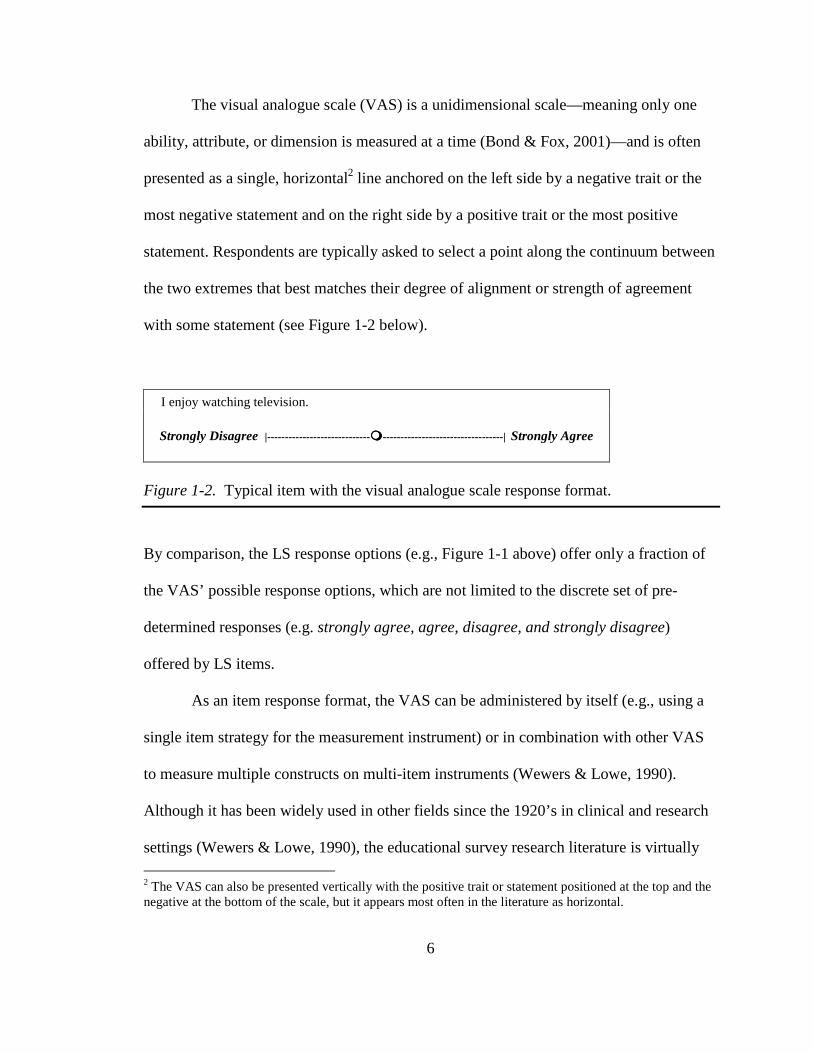
The visual analogue scale (VAS) is a unidimensional scale—meaning only one
ability, attribute, or dimension is measured at a time (Bond & Fox, 2001)—and is often
presented as a single, horizontal2 line anchored on the left side by a negative trait or the
most negative statement and on the right side by a positive trait or the most positive
statement. Respondents are typically asked to select a point along the continuum between
the two extremes that best matches their degree of alignment or strength of agreement
with some statement (see Figure 1-2 below).
I enjoy watching television.
Strongly Disagree |-----------------------------����----------------------------------| Strongly Agree
Figure 1-2. Typical item with the visual analogue scale response format.
By comparison, the LS response options (e.g., Figure 1-1 above) offer only a fraction of
the VAS’ possible response options, which are not limited to the discrete set of pre-
determined responses (e.g. strongly agree, agree, disagree, and strongly disagree)
offered by LS items.
As an item response format, the VAS can be administered by itself (e.g., using a
single item strategy for the measurement instrument) or in combination with other VAS
to measure multiple constructs on multi-item instruments (Wewers & Lowe, 1990).
Although it has been widely used in other fields since the 1920’s in clinical and research
settings (Wewers & Lowe, 1990), the educational survey research literature is virtually
2 The VAS can also be presented vertically with the positive trait or statement positioned at the top and the negative at the bottom of the scale, but it appears most often in the literature as horizontal.

7
silent on the VAS. Moreover, of the published studies that have involved VAS items or
indices, the vast majority have focused on adult populations (e.g., 18 and older) and
results can not necessarily be extrapolated to K-12 populations (e.g., younger than 18).
Moreover, it remains to be seen whether results observed in studies with adults are
constant over different measurement contexts (such as schools), respondent groups (such
as K-12 students), or traits (such as identification with school).
Research Purpose
In addition to the gap in the current K-12 educational survey research literature
about students’ reaction to the visual analogue scale, very little is known in any field of
research about how children respond to Web-based surveys with VAS response options.
Further, it remains unknown whether they will respond differently to VAS items online
than they would have had they been presented with LS items instead. The purpose of this
study was to contribute to the literature in K-12 educational survey research by
comparing a previously validated and highly reliable LS survey3 to the same survey with
VAS response options instead. Both versions of the survey administered in this study
were Web-based and both had the same number of items and same prompts but with
different response option formats. The LS version’s response options were presented as
radio buttons with choices such as “Strongly Agree” or “Disagree” and the VAS version
had slider-type response options presented with only the two extreme verbal cues of the
3 Meaning that the survey was originally comprised of items with LS response options.
8
LS (e.g., Strongly Disagree and Strongly Agree) on each end of a continuum.
Respondents used their mouse to click anywhere on the continuum and a marker
appeared that could be manipulated (slid) in either direction to indicate varying degrees
of “agreement” or “disagreement” with the item prompts.
The purpose of this study was to explore whether the VAS could be a more
suitable alternative to the Likert scale to frame response options for survey research in a
K-12 setting. The construct measured in this paper (and thus the subject for the LS vs.
VAS comparisons) was student identification with school, which has been examined in a
number of studies and measured using a number of Likert-scaled instruments.
Researchers involved in empirical studies of this construct have, to date, not explored the
possibility that the survey they administered might have yielded different results had a
continuous scale such as the VAS been used instead of the LS. Thus, this study compared
LS and VAS versions of the established scale, Identification with School Survey (Voelkl,
1996) to determine if the survey’s results (e.g., summated scale score) and psychometric
indicators (e.g., reliability and factor structure) were comparable, irrespective of the
response format. Further, because age had been shown in previous studies to be a
significant factor in children’s performance on surveys (Cremeens, Eiser, & Blades,
2007; Read & MacFarlane, 2006; Shields, Cohen, Harbeck-Weber, Powers, & Smith,
2003; van Laerhoven, van der Zaag-Loonen, & Derkx, 2004), the effects of age (using
school level as a proxy) and item response type were examined in an effort to determine
if there were any significant differences between how younger students and older
students responded when presented with VAS vs. LS response options.

9
Research Questions
Evidence has been presented that suggests Likert scale (LS) response options can
misrepresent the variability in students’ attitudes/beliefs by artificially grouping students
into a limited set of discrete categories that may not accurately reflect individual
responses. Additionally, evidence has been presented that suggests the visual analogue
scale (VAS) may be a more suitable survey response option for researchers to use due to
its continuous scaling, which offers a more sensitive measurement of attitudes/beliefs and
a much less restricted response range for students to individualize their responses.
Evidence has also been presented that suggests children’s age is an important factor to
consider when selecting an item response format because younger children’s cognitive
development is less developed than older children’s, which could impact the former’s
ability to accurately self-report. Lastly, evidence has been presented that suggests the
VAS may have an advantage over the LS on a Web-based survey due to its ability to
communicate an interval continuum to respondents that may yield greater score
variability and possibly greater score reliability.
Given that no previous studies have been conducted in educational survey
research to directly compare the LS to the VAS on a web-based survey with a K-12
student population in a school setting, the best method of framing response options in
educational survey research remains unclear. Consequently, this study seeks to
contribute to the literature by addressing the following research questions:
1. Does the response format change the factor structure of the survey?
2. Does the response format affect the reliability coefficient?
10
3. Are there significant mean differences for the summated scores overall between the LS version and the VAS version of the survey?
4. Are there significant mean differences of the summated scores on the LS and VAS versions of the survey between Elementary, Middle, and High School students?
5. Is there a significant interaction between level of schooling and item response type? If so, is it dependent on item response type?
Significance of the Study
The results of this study could provide answers to questions that have thus far
been overlooked in educational survey research. Further, the results of this study could
have implications for social scientists, particularly those whose survey research is used to
influence policy directly or indirectly affecting the lives of children. Moreover, because
results could have some bearing on children’s self-reports, in general, and for future
measures designed for students in elementary, middle, and high schools, in particular, the
results of this study could influence ways in which survey research is conducted in
tomorrow’s K-12 classrooms.
Summary
A standard tenet in research is that conclusions based on computed statistical
values are valid only insofar as the data used to calculate these values were collected in
an appropriate manner. Some critics have argued researchers run the risk of drawing
11
unwarranted conclusions when they rely exclusively on LS categorical surveys because
yielded data may not have been obtained using the most appropriate4 method (Brunier &
Graydon, 1996; Ohnhaus & Adler, 1975; Svennson, 2001; Wewers & Lowe, 1990). This
line of thinking stems from the view that LS items limit a respondent’s ability to
accurately or precisely express his or her opinions and therefore are not capable of
providing tenable evidence about varying degrees of agreement/disagreement or of
capturing the more subtle nuances of personal expression (Flynn, van Schaik, & van
Wersch, 2004). To that end, an LS survey’s validity and reliability could be called into
question. Moreover, since the quality of any research study is heavily dependent upon
the researcher’s ability to collect and interpret valid and reliable data, it could be argued
the LS may serve to restrict or implicitly limit attempts to achieve an accurate estimate of
the construct being measured, which, in turn, may also confound data interpretation or
otherwise impinge on sound decision making. This raises important questions about the
extent to which LS survey results used in educational research can be used to make
inferences about students or their schools.
The importance of accurate information is imperative in all fields of research, and
educational survey research is no exception. With the demand for data-driven decision-
making in today’s high stakes educational environment, it is imperative the instruments
used in data collection are as accurate and useful as possible. Given the limitations
mentioned above, the LS’ ability to provide researchers with the most accurate data is
4 Appropriate in this context refers to the scale’s ability to accurately measure the substantive construct or variable of interest.

12
questionable and therefore may not be the best possible or most appropriate choice for
measuring respondents’ attitudes or opinions in empirical educational research.

13
Chapter 2: Literature Review
Introduction
Today, survey research includes a broad range of methods for gathering data,
ranging from the more traditional one-on-one interview conducted in-person or on the
phone, to the more progressive, self-administered surveys such as those that capitalize on
today’s technology to collect responses via text-messaging or the Internet. Researchers
have used surveys for many years and although myriad forms have been proposed and
tested over the last century, the Likert scale is still by far the most widely used technique
for scaling item response options (Lange & Soderlund, 2004; OhnHaus & Adler, 1975;
Polit, 2004). This chapter proposes to focus specifically on measurement issues as they
relate to surveys in general, and the Likert scale (LS) and visual analogue scale (VAS), in
particular. The chapter concludes with a discussion of challenges related to surveying
children using LS and VAS response options as well as with an overview of issues
related to Web-based or online surveys.
Measurement Issues in Educational Survey Research
In the social sciences, one of the most frequently cited definitions of measurement
has been that of Stevens (1946). Stevens broadly defined measurement as the
assignment of numbers to aspects of objects or events according to one or another rule or
convention. In survey research, there is an ongoing debate about which scaling “rule or

14
convention” is most appropriate for use in the measurement procedure to ensure accurate
results and the meaningful interpretation of survey scores. Unlike most physical
scientists, social scientists tend to deal mostly with unobservable constructs that cannot
be directly measured. Survey researchers, in particular, must therefore rely on
psychometric theory to measure subjective phenomena such as attitudes. Psychometrics
is the field of study concerned with the theory and technique of measurement in
education and psychology, which includes methods such as the operationalization of
variables for the purposes of measurement and the scaling of attitudes. According to
Bowling (2005b),
Psychometric theory dictates that when a concept [or construct or variable]
cannot be measured directly…a series of questions that taps different aspects of
the same concept need to be asked. Items can then be reduced, using specific
statistical methods, to form a scale of the domain of interest, and the resulting
scale tested to ensure that it measures the phenomenon of interest consistently
(reliability), that it is measuring what it purports to measure (validity), and is
responsive to relevant changes [sensitivity] over time. (p. 344).
The primary purpose of conducting a survey is to enable the researcher to
examine some characteristic or trait as it relates to the people being surveyed and/or the
phenomena about which the people are being asked (Fink, 1995). If the researcher’s
conclusions are to have merit, they must be based on reliable scores obtained from valid
surveys. As with any research study, dependable results are contingent upon the
researcher’s ability to collect valid and reliable data that provide an accurate estimate of
15
the construct, characteristic, or attribute being measured (Litwin, 1995). In other words,
to be dependable, the survey instrument must measure what it was designed to measure
and provide a consistent estimate of what is actually being measured, intended or
otherwise (Linn & Miller, 2005; Nunnally, 1978). In survey research, the unintended or
unaccounted for measurements (or those “otherwise” measurements) are cause for
concern because they constitute measurement error.
Survey Errors
Researchers strive for, but fail to achieve, error-free measurement. Unfortunately,
perfect measurement does not exist. In many cases, “substantial mismeasurement
[remains] no matter how much care and expense is devoted to measuring the variable in
question” (Gustafson, 2004, p.3). Two types of error associated with survey research, in
general, and measurement, in particular, are random errors and systematic (or non-
random) errors. The first, random errors, are errors without qualification. Random error
(also known as random variation) represents differences in a variable due to chance rather
than to one of the other variables being studied. Although random variations tend to
cancel one another out in the long run, these types of error are not under the control of the
researcher and therefore were not examined in this dissertation. The second type of
errors, non-random errors, are those that are consistent or not random and therefore
should (or could) ostensibly be controlled or eliminated by the researcher. Controlling or
eliminating systematic errors is important because, as Blalock, Wells, and Carter (1970)
argue, "the existence of…nonrandom measurement errors becomes a serious problem for

16
inference in any study that is designed to go beyond merely locating correlates of a
particular dependent variable" (p. 76). Given that this dissertation aspires to examine
inaccuracies or errors resulting from possible design limitations or flaws in the
measurement instrument,5 in general, and errors related to response option design or
scaling technique, in particular, this study focuses exclusively on non-random errors.
In addition to random and non-random errors, there are several other types of
errors often associated with surveys including sampling error, coverage error, non-
response error, and measurement error. The first two essentially relate to errors
involving the sampling method or approach to contacting participants. These are
methodological errors not associated with the survey instrument itself; therefore, they
were not examined. The third, non-response errors, are a function of the respondent and
were not examined in this dissertation. The fourth, measurement error, is error that occurs
when the observed value is different from the true6 or actual value of the measured
variable. In terms of this study, these types of survey research errors were defined as
those associated with the measuring instrument itself—as contrasted with other sources
of measurement error—and were the only type of survey research error examined in this
dissertation.
Reliability.
Reliability refers to the extent to which a measure or score is repeatable and
consistent and free from random errors. Put another way, it is a measure of how 5 As opposed to “flaws” in the respondent. These respondent-based errors include instances such as when respondents do not understand the question or cannot remember the relevant information, or when they strategically edit responses in a misleading way before reporting (or selecting) them. 6 The true value is a hypothetical value that is yielded if a variable were perfectly measured (e.g., without error).
17
reproducible a survey’s data are (Litwin, 1995). Crocker and Algina (1986) remind us,
“reliability is a property of the scores [italics added] on a test for a particular group of
examinees” (p. 144) and not of the test or survey itself. Therefore, it is inappropriate to
refer to an instrument as either “reliable” or “unreliable.” Alwin (2007) expounds on the
importance of reliability as it relates to measurement by observing:
reliability is not a sufficient condition for validity, but it is necessary, and
without reliable measurement, there can be no hope of developing scientific
knowledge. The obverse of this logic is that if our measures are unreliable they
are of little use…[for] detecting patterns and relationships among variables of
interest. Reliability of measurement is therefore the sine qua non of any empirical
science” (p. 16).
There are several types of reliability analyses that can be conducted to estimate a
reliability coefficient for a test or survey including alternate-form, inter-observer, intra-
observer, test-retest, and internal consistency reliability. In this study, only one form was
administered, therefore alternate-form reliability does not apply because, according to
Crocker and Algina (1986), “the alternate form method requires constructing two similar
forms [e.g., with equivalent but not identical items] of a test and administering both
forms to the same group of examinees” (p.132). Inter-observer or interrater reliability is
not relevant to the study either because the study does not examine the extent of
agreement among two or more independent raters judging the same phenomena.
Similarly, intra-observer reliability is not relevant to the study because it refers to the
extent to which an individual observer is consistent in her observational codings if she
18
twice codes (rates) an object or occurrence (e.g., student essay or video of a teacher’s
response to classroom disruption).
Test-retest reliability (rxx′) is a common indicator of response consistency. Often
referred to as a co-efficient of stability, it is defined as the consistency of measurement
based on the correlation between test and retest scores for the same individual. Typically,
the same test is administered twice to the same people after a period of time and after the
retest, two scores on the same measure for each person are generated and the correlation
between the scores is obtained. Depending on the type of data being analyzed, the
researcher will either apply Pearson r or Spearman rho on the total scores of the two
administered tests or surveys.
Internal consistency estimates of reliability (ICR) are applied to groups of survey
items (as opposed to single items) thought to measure different aspects of the same
construct (Litwin, 1995). Cronbach (1951) defined a survey with high internal
consistency as one comprising positively intercorrelated items and not necessarily one
reflecting a high degree of unidimensionality. To measure ICR, Cronbach’s coefficient
alpha (α ) is generally calculated as an index of a survey’s internal consistency, which is
determined by “the ratio of the sum of the item covariances to the total observed score
variance” (Crocker & Algina, 1986, p. 153). Although there are other ways to measure
ICR besides Cronbach’s alpha, evidence suggest they all arrive at essentially the same
estimates of reliability (Pedhazur & Pedhazur Schmelkin, 1991).
19
Ordinal vs. Interval Measurement
It is important for the researcher to bear in mind that the type of measurement
scale used to take measures will affect the validity, reliability, and usefulness of the data
collected. With Likert scale (LS) surveys, there is a general lack of consensus on whether
they should be treated as ordinal- or interval-level measurement, and rightfully so. In
social science research, the distinction between the two is often blurred.
Ordinal Measurement Scale
Ordinal measures require that “…the objects of a set can be rank-ordered on an
operationally defined characteristic or property” (Kerlinger, 1992, p.399). This means, in
general, a hierarchy is in place to “rank” responses from a lesser or lower degree to a
more or higher degree of some specified characteristic. For example, strongly agree is a
“higher” degree of affirmation than agree, therefore strongly agree would be assigned a
higher numeric value than agree. Although intervals are implied by these varying
degrees of verbal categories as well as by the numeric values often assigned,
traditionalists argue an ordinal scale’s intervals are purely arbitrary and therefore no
meaning can be attached to the size or distance between measurements and no meaning
can be attached to the shape of the set of measurements’ frequency distribution (Gardner,
1975). Traditionalists further maintain only non-parametric statistics can be used with
ordinal scales because they do not require the estimation of population values and no
assumptions are made about interval equivalencies or the shape of the distribution of
population scores (Armstrong, 1981).

20
Interval Measurement Scale
To qualify as an interval measure, the scale must represent “equal distances [or
intervals] in the property being measured” (Kerlinger, 1992, p.400). As such, relative
sizes of the intervals between two different measurements along the scale can be
meaningfully interpreted and meaning can be attached to the frequency distribution’s
shape (Gardner, 1975). In addition to their capability of providing a more precise
estimate than ordinal measures, interval measures have the added benefit of enabling the
researcher to use more powerful parametric statistical techniques (Kerlinger, 1992;
Labovitz, 1970).
In attempting to decide whether to treat data as ordinal or interval, researchers
face the potential loss of information because of the limited resolution of ordinal
measurements. Kriege (1999) calls this an issue of “scale coarseness” and argued it
causes biases that “…can affect the mean, variance, covariance, correlation coefficient,
and the reliability of the scores” (p.763). Moreover, since ordinal scales offer only a
“coarse” estimate, they can potentially impact the internal consistency, test-retest
reliability, and concurrent and predictive validity of a survey (Champney & Marshall,
1939; Bowling, 1998).
Treating ordinal data as interval.
A problem survey researchers routinely face is whether the use of more powerful
statistical techniques are justified with ordinal-level scales of measurement. To directly
address the issue of whether it is acceptable to use an interval scale when an ordinal scale
is, by definition, more appropriate, Labovitz (1970) conducted an empirical investigation
21
in which he manipulated ordinal (e.g., ranked) data from a previously published study7
and substituted his own equidistant (linear), monotonic numbers and randomly generated
numbers8 according to 18 different monotonic scoring systems. His results demonstrated
negligible error in comparison to the “true” scoring systems, which led Labovitz to
conclude:
(1) certain interval statistics can be used interchangeably with ordinal statistics
and interpreted as ordinal, (2) certain interval statistics (e.g., variance) can be
computed where no ordinal equivalent exists and can be interpreted with
accuracy, (3) certain interval statistics can be given their interval interpretation
with only negligible error if the variable is “nearly” interval, and (4) certain
interval statistics can be given their interval interpretations with caution (even if
the variable is purely ordinal), because the “true” scoring system and the assigned
scoring system, especially the equidistant system, are almost always close as
measured by r and r2 (1970, p. 523).
Thus, Labovitz (1970) argued, even though some “small error” may result from treating
ordinal variables as interval, doing so is justified because it enables the researcher to use
“more powerful, more sensitive, better developed, and more clearly interpretable
statistics with known sampling error” (p.515). While this may be true, Labovitz failed to
provide the researcher with guidance on when it is “worth the risk” to ignore the error
introduced when ordinal scales are treated as interval scales in favor of using advanced
7 Labowitz (1970) examined the relationship between occupational prestige (which is based exclusively on the principle of ordinal ranking) and male suicide rates. The data comprised prestige rankings of 36 U.S. occupations obtained from a 1947 national survey and suicide rates by occupation obtained from the 1950 U.S. Census. 8 The assigned numbers were all within the range of 1 to 10,000 and their assignments were all consistent with the ordinal ranking monotonic function.
22
statistical techniques. Moreover, he failed to mention this risk may be reduced or
eliminated altogether if a suitable alternative, designed for the interval scale, was used.
As Krieg (1999) suggested, “the simplest way to avoid the biases induced by coarse
measurement scales [e.g., Likert scales] is not to use them in the first place” (764).
Measuring Survey Responses
This section provides a general discussion about the two item response types that
are the focus of this dissertation: the Likert scale (LS) and the visual analogue scale
(VAS). The LS is presented first, followed by the VAS and then a discussion of whether
either is ordinal or interval level measurement follows. Each is discussed in terms of how
it captures a respondent’s survey responses and in terms of measurement error that results
due to item response format.
The Likert Scale
In his seminal monograph, Rensis Likert (1932) originally proposed that his scale
was a summated scale9 to be used to assess the attitudes of survey respondents. Although
technically the term Likert scale refers to a summated score produced by a survey
comprised of Likert-type items rather than to an individual item itself, the term Likert
scale (LS) is commonly used today to refer to the universal fixed format approach to
measuring attitudes—and more broadly to virtually any survey item with labeled, bipolar
9 “A scale or index made up of several items measuring the same variable. The responses are given numbers in such a way that responses can be added up [or summated]” (Vogt, 1999, p. 284).
23
(e.g., agree/disagree) response options typically delineated by a discrete set of monotonic
categories.
The LS format on a survey characteristically consists of an item prompt such as a
statement about the attitude being measured (e.g., I enjoy reading mystery novels)
followed by a limited or discrete set of responses designed to capture a respondent’s
personal opinion about (or attitude toward) the item prompt. Typically, the LS has four to
seven response options, each consisting of a single word or short phrase that differs by
varying degrees ranging from one negative extreme to its polar opposite positive extreme
(e.g. from strongly disagree to strongly agree or not at all likely to highly likely). From
the range of options presented, respondents are generally instructed to choose only one to
indicate their level or degree of agreement or disagreement with the statement presented
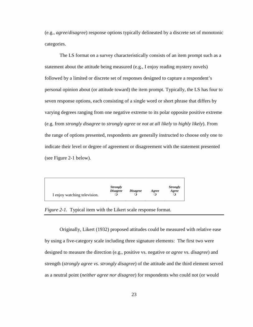
(see Figure 2-1 below).
Strongly Disagree Disagree Agree
Strongly Agree
I enjoy watching television. � � � �
Figure 2-1. Typical item with the Likert scale response format.
Originally, Likert (1932) proposed attitudes could be measured with relative ease
by using a five-category scale including three signature elements: The first two were
designed to measure the direction (e.g., positive vs. negative or agree vs. disagree) and
strength (strongly agree vs. strongly disagree) of the attitude and the third element served
as a neutral point (neither agree nor disagree) for respondents who could not (or would
24
not) choose between the options presented. He also advocated the use of including don’t
know as a response option so researchers could make distinctions between people who
had no opinion (or honestly did not know) and those who were genuinely neutral. While
there is no consensus on the optimal number of response options to use, it is fair to say
more researchers claim the ideal number is five (Lissitz & Green, 1975; Jenkins & Taber,
1977) or seven (Symonds, 1924; Grigg, 1980; Preston & Colman, 2000; Witteman &
Renooij, 2002) than any other number; and most agree an odd number is best to allow for
an “average” position on the scale (Grigg, 1980).
Response issues with LS items.
Because LS items are used so extensively in today’s surveys, respondents may go
into “auto pilot” mode when responding due to their over-familiarity with this format.
That is, respondents may be less apt to fully consider responses before selecting one of
the LS response options. This habitual response behavior might be avoided if respondents
were presented with a “cognitive speed bump” (Lange & Söderlund, 2004) such as an
alternative, less- commonplace item response format to force them to personally reflect
on what each question really means and how best to respond (see, for example, Gardner,
Cummings, Dunham & Pierce, 1998 or Shamir & Kark, 2004). Although the idea of
designing a survey incorporating a response format (e.g., the VAS) that somehow gets
respondents to pause and reflect rather than responding automatically makes sense
theoretically, I question whether the novelty or positive effect(s) would diminish over
time (or even over the course of the survey) as familiarity increases with each subsequent
encounter. Moreover, because the validity and long-term effects of this survey design

25
approach are, to date, unexamined in survey research, it remains unclear whether using
the VAS response option in place of the LS creates enough of a cognitive speed bump to
have a significant effect on a survey’s outcome or results.
Another common problem associated with LS items stems from a respondent’s
overuse of the mid-point (e.g., neither agree nor disagree or neutral response) or
apparent refusal to select one of the options presented because they do not accurately
reflect the response he/she wishes to convey (Brunier & Graydon, 1996). Holmes and
Dickerson (1987) suggested that the midpoint of an odd-numbered LS response set may
be an easy or “default” choice for respondents to make when they find it difficult to select
a response that precisely conveys how they feel or perhaps find the item prompt too
sensitive or painful to reflect upon. Under these circumstances, respondents typically opt
to: 1) skip the item, 2) write in their own response, or 3) indicate their response by
placing a mark between the options presented. As a result, data analysis can be
compromised as such responses must either be dropped or imputed. These types of
behaviors could potentially be avoided with an alternative response option that offers
respondents more freedom to personalize their responses and that has the potential to
achieve a more accurate estimate of the measured construct. One possible alternative that
gives respondents the freedom to express their personal opinions more precisely is the
visual analogue scale (Givon & Shapira, 1984).
26
The Visual Analogue Scale
The visual analogue scale (VAS) is a unidimensional scale—meaning only one
ability, attribute, or dimension is measured at a time (Bond & Fox, 2001)—and is often
presented as a single, horizontal10 line anchored on the left side by the most negative
statement or trait and on the right side by the most positive statement or trait.
Respondents are typically asked to select a point along the continuum between the two
extremes that best matches their degree of alignment or strength of agreement with some
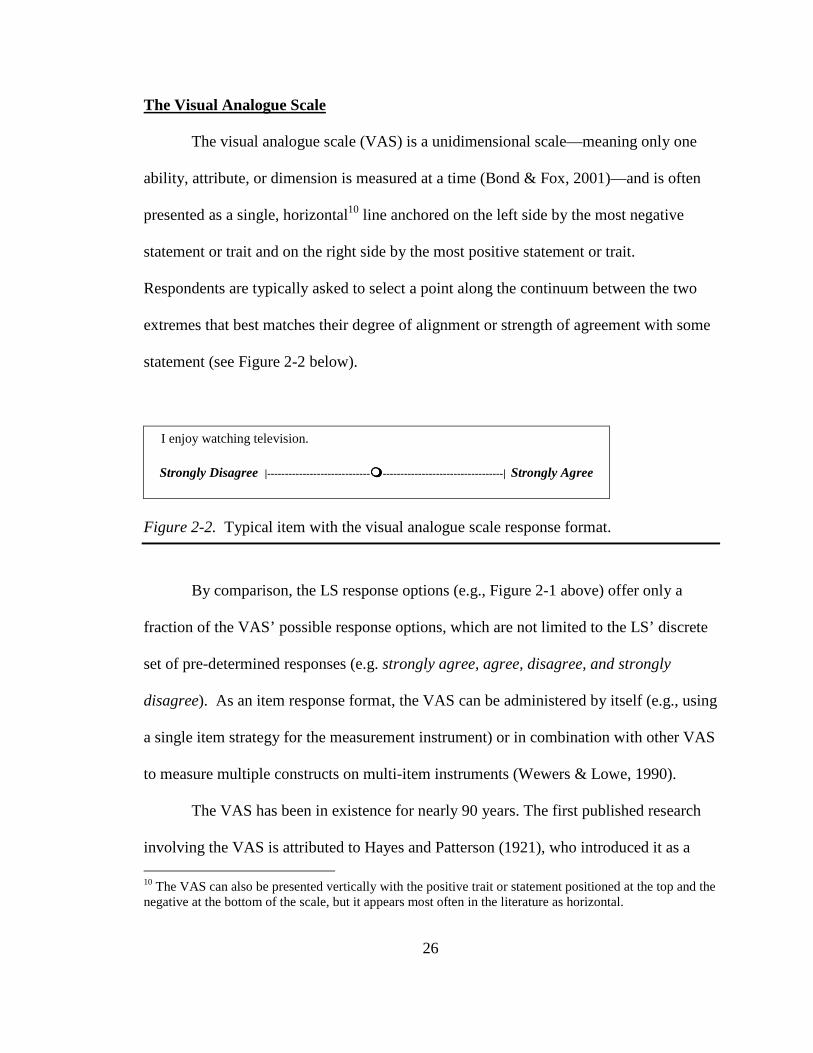
statement (see Figure 2-2 below).
I enjoy watching television.
Strongly Disagree |-----------------------------����----------------------------------| Strongly Agree
Figure 2-2. Typical item with the visual analogue scale response format.
By comparison, the LS response options (e.g., Figure 2-1 above) offer only a
fraction of the VAS’ possible response options, which are not limited to the LS’ discrete
set of pre-determined responses (e.g. strongly agree, agree, disagree, and strongly
disagree). As an item response format, the VAS can be administered by itself (e.g., using
a single item strategy for the measurement instrument) or in combination with other VAS
to measure multiple constructs on multi-item instruments (Wewers & Lowe, 1990).
The VAS has been in existence for nearly 90 years. The first published research
involving the VAS is attributed to Hayes and Patterson (1921), who introduced it as a
10 The VAS can also be presented vertically with the positive trait or statement positioned at the top and the negative at the bottom of the scale, but it appears most often in the literature as horizontal.

27
“new method for securing the judgment of superiors on subordinates” (p. 98) and extolled
the virtues of the VAS,11 which they described as “simple, self-explanatory, concrete and
definite” (p. 99). Although in the beginning, the VAS was used mostly for external-rater
or objective measurements (e.g. job evaluation or task performance), over the years, it
became increasingly associated with the measurement of subjective phenomena such as
“feelings, perceptions, or sensations [which are traditionally] difficult to measure on
scales with predetermined intervals [e.g. Likert scales]” (Lee & Kieckhefer, 1989, p.
128).
The bulk of the published research involving the VAS has been, to date, focused
on adult populations. Of this research, the most comprehensive and well-documented
studies involving the use of VAS are found in the medical or health-related field’s pain
literature, where it has been regarded as the best method or “gold standard” for the
subjective measurement of pain (Yarnitsky, Sprecher, Zaslansky, & Hemli, 1996; Scott &
Huskisson, 1976). In general, the pain literature involving adults has been mixed.
Proponents have argued that the VAS:
1. can have better responsiveness (i.e. ability to detect clinically significant change) than the Likert scale (Ohnhaus & Adler, 1975)
2. can yield a greater variation of scores and produce scores more normally distributed than LS formats (Brunier & Graydon, 1996; Grigg, 1980)
3. can be easy to understand and use—especially for non-native speakers and individuals with less-than-average reading ability (Pfennings, Cohen, & van der Ploeg, 1995; Ahearn, 1997; Kerlinger, 1992; Freyd, 1923)
4. may require little to no verbal or reading skill (Lee & Kieckhefer, 1989) 11 Hayes and Patterson (1921) referred to their scale as a “graphic rating method,” which, for all intents and purposes, is a VAS.

28
5. can be administrable in a variety of settings (Averbuch & Katzper, 2004)
6. can yield a more sensitive and accurate representation of the measured construct (Grant, Aitchison, Henderson, Christie, Zare, McMurray, et al. 1999; Sriwatanakul, Kelvie, Lasagna, Calimlim, Weis, & Mehta, 1983; Witteman & Renooij, 2002)
7. can be easy to score (Joyce, 1975)12
Conversely, critics of the VAS have presented less favorable views. Some studies have
shown respondents disliked VAS items because they are 1) “harder” than LS items; 2)
take more time to complete; and 3) require training because of their unfamiliar format
(Jaeschke, Singer, & Guyatt, 1990; van Laerhoven, et al., 2004; Williamson & Hoggart,
2004).13 Further, some researchers have presented evidence suggesting respondents may
find the VAS difficult to use because it requires them to think about responses in terms of
(or within) a “mathematical dimension” (Duncan, Bushnell, & Lavigne, 1989; Joyce,
Zutshi, Hrubes, & Mason, 1975).
Although it has been widely used in other fields since the 1920’s in clinical and
research settings (Wewers & Lowe, 1990), the educational survey research literature is
virtually silent on the VAS. Moreover, of the published studies involving VAS items or
indices, the vast majority have focused on adult populations (e.g., 18 and older) and
results can not necessarily be extrapolated to K-12 populations (e.g., younger than 18).
Moreover, it remains to be seen whether results observed in studies with adults are
12 Especially now that VAS can be administered via computer and scored electronically rather than by hand as with the paper-pencil versions. 13 It bears noting that the vast majority of these studies involved respondents that were at least 18 years old.
29
constant over different measurement contexts (such as schools), respondent groups (such
as K-12 students), or traits (such as identification with school).
Likert Scales: Ordinal or Interval?
Likert scales are a controversial “middle case.” Proponents of the use of interval
measurement of LS response options argue that
although most measures used in sociobehavioral research are not clearly on an
interval level, they are not strictly on an ordinal level either. In other words, most
of the measures used are not limited to signifying “more than,” or “less than,” as
an ordinal scale is, but also signify degrees of differences, although these may not
be expressible in equal interval units (Pedhazur & Schmelkin, 1991, p. 28).
Technically, data obtained from fully anchored LS (e,g., all response options are
labeled and arranged as fixed anchor points from Strongly Disagree to Strongly Agree)
are considered to be inherently ordinal because respondents most likely do not uniformly
perceive the specified anchors as forming equal intervals (Goldstein & Hersen, 1984).
Critics of the legitimacy of claiming the LS can be measured at an interval level maintain
that the degrees of separation between terms do not represent equal units (Williamson &
Hoggart, 2004), which would, of course, mean data obtained via mathematical averaging
would be untenable.
Since, traditionally, the numbers assigned to Likert response options are arbitrary
(e.g., 1-5) and do not have any meaningful connection to the responses they represent
(Hasson & Arnetz, 2005), one cannot assume the difference between Agree and Strongly
30
Agree is equal to or the same as the difference between Disagree and Strongly Disagree.
This is not to say the numbers associated with LS response options do not have meaning,
it is just their meaning is not very precise because they do not represent “like quantities.”
For example, with a quantity such as dollars, the difference between $1 and $2 is the
same as between $2 and $3. This is not really the case with numbers associated with LS
response options. For example, if a survey item has four response options, researchers
can be sure nearly all respondents understand a rating of two (Disagree) is between a
rating of one (Strongly Disagree) and a rating of three (Agree), but they cannot be sure
respondents interpret that Disagree lies precisely halfway between Strongly Disagree and
Agree. This is also true with an odd number of LS response options (e.g., five or seven)
where, for example, the mid-points of the scale are often presumed to be “neutral,”
meaning Neither Agree nor Disagree. Here, one cannot be sure respondents interpret that
this response option lies precisely halfway between Strongly Disagree and Strongly
Agree or that respondents do not have even a slight preference toward one or the other.
For example, if a respondent does not fully Agree with the item prompt but is forced to
choose a response, he may decide the next lower option serves as a better indicator.
Thus, this respondent’s overall or summated score will be negatively biased or lower than
it should be.
Depending on the frequency with which this biasing effect occurs over the course
of an entire LS survey, a respondent’s summated score may be significantly different
from what it would be if he were given the opportunity to respond with an interval-level
31
response option such as the VAS,14 for example. In cases such as these, the LS fails to
accurately capture respondents’ true intentions because it assumes a single interpretation
of all response options when respondents may (and most likely do) have varying degrees
of Agree-ment in mind when selecting their responses.
Visual Analog Scales: Ordinal or Interval?
VAS responses are not as constrained as LS responses because technically, the
VAS are continuous scales of measurement essentially offering an infinite number of
places along the line to indicate one’s response as opposed to the LS’s typically limited
four to seven responses (Noel & Dauvier, 2007). Although in practice, researchers tend to
divide the VAS line up into an ordered, defined number of segments to make it easier to
measure or score survey responses, respondents do not see these divisions in an effort to
promote the perception and interpretation that the VAS line is a continuous response
format. With the possibility of constructing online versions of surveys, previous
recommendations based on paper-based surveys with VAS response options no longer
apply. For example, according to several empirical studies involving paper-based VAS
surveys, researchers have used varying lengths ranging from 5cm to 10.5cm, although
100mm (or 10cm) is most often used because it can be broken into 100 equal segments of
1mm each15 (Grigg, 1980). However, when presented online for Web-based surveys, the
length of the VAS line is difficult to standardize due to differences in screen sizes, video
14 Of course, it bears noting that while the intervals in a VAS are considered equidistant, they may in fact not be equal in terms of intensity of a person’s belief or her interpretation of the scale. 15 Or 10 equal segments of 1cm each.
32
modes, settings, etc. Thus, pixels are likely to become the best unit of measurement.
Another former problem associated with paper-based VAS items was the quantification
of results, which required manual measurement (e.g., with a ruler) of each response for
every survey. As you can imagine, this could present a huge burden to researchers,
especially with large samples, not to mention problems with accuracy in measuring the
precise distance from one end of the continuum to where the respondent placed his/her
mark. This problem is all but eliminated with Web-based surveys because absolute
judgments about where respondents place their marker are made possible via computer-
programmed calculations yielding its precise location16 along the VAS line, resulting in
increased sensitivity and reliability of scores (Funke & Reips, 2007; Noel & Dauvier,
2007) in addition to faster scoring and retrieval of results for researchers.
To explore the impact on data quality and the measurement error of the VAS
response option when administered online, Funke and Reips (2007a) conducted four Web
experiments. In the first experiment, they demonstrated data from the VAS approximate
the interval scale (e.g. equidistant) level and concluded the VAS should be used to
measure continuous variables and parametric statistical tests are duly warranted. In
experiments two and three, they compared LS items to VAS items and found the LS
differs “systematically” from interval level and produces ordinal level data only. Their
fourth experiment examined test-retest reliability of the VAS and LS by repeatedly
administering a 40 item personality inventory and concluded, “although VAS facilitate a
16 The degree of precision is limited only by the number of decimal points the researcher chooses to employ in the calculations.
33
far more precise judgment, there was no negative influence on retest reliability” (Funke
& Reips, 2007a, p. 10).
Children and Surveys
The subjective and multidimensional nature of phenomena such as feelings,
attitudes, or sensations can present particularly challenging measurement difficulties
when working with children, especially younger children, because they are often limited
developmentally in their abstract and verbal abilities (Tesler, Savedra, Holzemer, Wilkie,
Ward, & Paul, 1991). According to Chambers and Johnston (2002), using and responding
to rating scales accurately is a difficult developmental task for younger students. While
the literature is inconclusive about whether it is appropriate to use chronological age as
the primary or sole determinate of a child’s ability to use scales such as the LS and VAS,
doing so appears to be the prevalent method used by the majority of researchers (Shields,
Palermo, Powers, Grewes, & Smith, 2003). A conventional alternative to using
chronological age is to use cognitive development as a predictor of children’s ability to
use various scales successfully.
Cognitive Development
Piaget’s concrete operations vs. formal operations.
Piaget conceptualized cognitive development as a series of periods or stages
characterized by qualitatively different abilities (Piaget, 1970). Although Piaget identifies
four stages of cognitive development, only his latter two stages—concrete operations and
34
formal operations—are applicable to this dissertation because the sample only included
children ages 9 through 18.17
Piaget proposed children’s thought processes gradually become organized and
integrated with one another into larger systems of thought processes. These systems—
known in Piagetian terminology as operations—allow children to pull their thoughts
together in a way that makes sense, and thus to think logically. Such integrated and
coordinated thought processes emerge at the beginning of the concrete operations stage.
Although they are capable of many forms of logical thought and can exhibit many signs
of logical thinking, their cognitive development is not yet complete and thus children in
this stage of cognitive development (generally 7 to 11 years old) may find it difficult to
grasp hypothetical scenarios that they cannot directly observe or experience or that are
not true-to-fact. They may also have difficulty understanding abstract ideas or notions
(e.g., democracy, human rights) and struggle with proportional reasoning or mathematical
concepts such as infinity or negative numbers. These cognitive “limitations” could have
an impact on a concrete operational child’s ability to grasp the concept of the VAS
response format, given that it is presented as a continuum (although no studies to date
have investigated the legitimacy of this claim). To that end, this group of students may
actually prefer the LS given its “concrete” presentation of verbal anchors or descriptors
that could serve as a guide or signpost with which they could identify. This would
support the findings of van Laerhoven, van der Zaag-Loonen, and Derkx (2004), who
17 See Chapter 3 for a description of the sample and inclusion/exclusion criteria.
35
found that when surveying children18 (ages 6-18, n=120) about their feelings19 and
opinions20 the younger children (6-12) preferred the Likert scale over the VAS because
they thought it was “easier to complete.”
As children progress to the fourth and final stage, formal operations (generally 12
years old and above), they begin to be able to think about concepts having little or no
basis in concrete reality—concepts that are abstract, hypothetical, or contrary-to-fact—
and they become more independent thinkers capable of unique self-expression.
Furthermore, children in the formal operations stage begin to recognize what is logically
valid is different from what is true in the real world. A number of abilities essential for
sophisticated mathematical reasoning also emerge in the formal operations stage that
enable these children to use and understand proportions, ratios, and continuums in their
reasoning. This would suggest students in the formal operations stage would not only
understand the VAS, but may prefer it over the LS due to the ability of the VAS to allow
them to convey precisely how they feel.
Children’s Ability to Self-Report
While there are many important factors to keep in mind besides item response
format when both designing and administering surveys for children (e.g., item phrasing,
number of items, time constraints), it has been suggested the rater’s (respondent’s)
competence to self-report is the most important of all (Guion, 1986; Cronbach, 1990). 18 This study took place in the Netherlands and the subjects were described as either” immigrants (first, second or third degree non-native children) and native Dutch children” (van Laerhoven, van der Zaag-Loonen & Derkx, 2004, p. 831). 19 These items asked the children about their feelings about dreams and their current mood. 20 These items asked the children about school, sports, and height.

36
Research suggests children as young as 8 years old are able to provide reliable reports on
their well being (Rebok et al., 2001). However, asking children using survey-style
questions may be a major challenge especially with younger children because their views
and opinions are often “black and white,” meaning no “shades of grey” exist in their
views. Thus, younger children tend to respond to scale questions by selecting extreme
values (e.g. very satisfied or very unsatisfied). Another challenge is that children’s verbal
and reading abilities have much more variability than those of adults and they often
interpret response choices literally. As a result, survey items must be reviewed with the
utmost care to ensure words used have the same meaning for all participants (Shields,
Palermo, Powers, Fernandez, & Smith, 2005). Even though there is no perfect solution to
all the problems arising from conducting surveys with children, most experts recommend
that surveys are kept short because children tend to have short attention spans and that the
survey is fun and administered in a child-friendly environment. Additional issues needing
to be taken into consideration when conducting survey research with children include:
(1) the level of literacy/reading level of respondents; (2) their tendency to want to choose
a response they think will please the researcher rather than what they, themselves, truly
feel; and (3) their responses tend not to be reliable over time (Borgers, Hox, & Sikkel,
2003).
37
Children and Likert Scales vs. Visual Analogue Scales
VAS have been used to assess the strength of perceptions of children in many
clinical and research settings. While numerous studies have used the VAS with children
(e.g., Champion, Goodenough, von Baeyer, & Thomas, 1998; Goodenough, Addicoat,
Champion, McInerney, Young, Juniper, et al., 1997; Svensson, 2000), and several have
demonstrated the ease of use, effectiveness, and sensitivity of the VAS when used with
children (Abu-Saad, 1984; Abu-Saad & Holzemer, 1981; Abu-Saad, Kroonen, &
Halfens, 1990; Berntson & Svensson, 2001), results tend to be mixed with regard to
children’s opinions about using the VAS. For example, some studies on pain experience
in children found that they preferred the VAS over a Likert-type response option because
of its specificity and accuracy (Stinson, Kavanagh, Yamada, Gill, & Stevens, 2006) and
because the VAS “felt the most free to answer” and allowed them to “put a mark
wherever [they] want” (Berntson & Svensson, 2001, p. 1134);21 whereas others found
children, regardless of age, preferred the LS response option to the VAS because it was
“easiest to complete” (van Laerhoven, van der Zaag-Loonen, & Derkx, 2004)22 or
because it provided “more choices” (Rebok et al., 2001).23 In theory, children with less
reading potential such as younger children or children with limited English (or majority 21 This study involved Swedish children 2-18 years old (n=26) suffering from juvenile chronic arthritis and examined their perception of pain using three different scales: VAS, graphic rating scale (which is like the VAS but has word descriptors at specified points beneath the line), and a 4-point verbal descriptor scale (which is essentially a Likert scale with more detailed response options). Results of this study should be interpreted with caution due to its small sample size. 22 This study involved Dutch children 6-18 years old (n=120) and examined their preference for the LS, VAS, or a 10-point numeric rating scale. It also asked the children to evaluate the level of difficulty they had with each response type. The questionnaire used in the study asked basic questions about students’ dreams, frequency of riding the bus to school, views on sports, television, and school, and about students’ general feelings. 23 Due to its small sample (n=19), conclusions from the Rebok et al. (2001) study should be interpreted with caution and perhaps considered tentative, at best.
38
language) proficiency would be more likely to prefer VAS response options because
VAS response options generally require shorter reading times and less sophisticated
reading skills than LS response options; however, as van Laerhoven, et al. (2004)
reported, these groups differed as well with younger, native Dutch children preferring the
Likert scale due to its ease of use and “non-native” immigrant children preferring the
VAS because they found it to be simple and made filling out the survey easier for them.
VAS and Children
As with studies involving the use of VAS with adults, the most comprehensive
and well-documented studies involving the use of VAS with children are found in the
medical or health-related field’s pain literature. Here the VAS is often used as a pain
scale and is presented in a number of formats including: 1) the basic, horizontal VAS line
(e.g., Figure 2-2 above), or 2) the basic VAS with verbal descriptors along the line and
sometimes scale marks dividing the line into distinct segments,24 or 3) the strictly non-
verbal VAS format, which typically presents the basic horizontal VAS line with
illustrations or faces in varying degrees of distress on each end of the continuum (as
opposed to verbal descriptors such as “strongly disagree” on one end and “strongly
agree” on the other). With the non-verbal format, which is typically used with children
too young to read, the child rates her degree of pain or discomfort, for example, by using
the facial expressions on either end as indicators of where to mark her response on the
VAS to indicate her current state, where no pain is typically indicated by a smiling face
24 Some authors refer to this type of VAS as a “graphic rating scale” or GRS

39
and pain as bad as it ever can be is typically indicated by a frowning, crying face (Lee &
Kieckhefer, 1989). In addition to measuring the intensity of pain, the VAS has been used
to measure the frequency of pain. Figure 2-3 below depicts a hybrid of the verbal and
non-verbal visual analogue scales that includes both verbal and visual cues. This item
was one of several used along with cognitive interviewing to examine school-aged
children’s self-reported health (Rebok, et al. 2001).
Figure 2-3. Pediatric health status questionnaire item measuring the frequency of stomachaches for children 6-11 years old.
Interestingly, much of the pediatric pain research literature demonstrates the same
measure or scale should not be used with all types of pain, in all types of circumstances,
or with all types of children’s populations. In their extensive review of self-report pain
measures for use in clinical trials in children and adolescents (ages 3-18), Stinson,
Kavanagh, Ymada, Gill, and Stevens (2006) sought to identify only well-established
measures that met a priori criteria of having sound empirical evidence of their reliability,
validity, responsivity, interpretability, and feasibility. Of the more than 30 pediatric self-
report pain intensity scales they identified, only six—one of which was the VAS—met all
of the inclusion criteria (see Stinson et al. 2006, p. 147 for exclusion rationale). The
results of this study led the authors to conclude that of the six measures included in their
40
review, “no single scale was found to be reliable and valid across age groups or pain
types” (p. 153). This evidence suggests children of different ages (where age is a proxy
for developmental level) can be expected to self-report effectively or accurately with
various response formats as long as the instruments used are age appropriate and
appropriate according to the children’s cognitive development and ability. This
corresponds to the findings of several other studies that suggest that age, cognitive
development, and cognitive ability are the best predictors of whether a child is capable of
using scales such as the VAS or LS (Cremeens, Eiser, & Blades, 2007; Malviya, 2006;
Shields, Palermo, Powers, Grewes, & Smith, 2003). These findings also suggest the use
of the LS may not be appropriate across all grade levels or ages or across all contexts or
constructs as it is often used presently.
VAS and children’s ability to understand measurement and scale.
Duncan, Bushnell, and Lavigne (1989) maintain that “non-verbal tests, such as the
visual analogue scale require a person to imagine his pain in terms of a mathematical
dimension, a task that may be difficult…especially for some age groups” (p. 301). Given
the typical design of the VAS, with its presentation of a continuum between two
diametrically opposed verbal or visual descriptors (e.g., strongly disagree/strongly agree,
never/always, ☺/�), children need to have at least a basic understanding of how to
convey an intrapersonal physical or emotional experience, for example, within the
parameters of a linear or mathematical format. That is, children need to be able to
connect what they are feeling with what it means to place a mark on the VAS closer to
41
one end of the line versus the other end. This skill requires the use of analogy and
proportional or spatial reasoning and the use of estimation.
Research has shown that children as young as three and four years old
demonstrated analogical reasoning and an understanding of proportional reasoning
(Goswami & Brown, 1989; Singer-Freeman and Goswami, 2001); however, in order to
use the VAS effectively, children must also be able to form an estimate of what they are
feeling, for example, and to quantify that estimate in terms of its linear magnitude or
proportion of the VAS line that best expresses their feeling.
According to Sowder (1992), in order to form an estimate, “one must have a
mental reference unit, that is, a mental ‘picture’ or ‘feel’ for the size of the unit” (p. 371).
Thus, children using the VAS need to be able to establish a “mental reference unit” of the
pain they are feeling, for example, and visually estimate its magnitude in relation to the
VAS line. This process has been facilitated by the use of verbal or visual end-point
indicators on the VAS line that children can connect with. Rebok et al. (2001)
demonstrated that children as young as five years old were able to use the VAS
effectively when illustrated characters were used with whom children could identify and
“who illustrated the health concept…used to anchor each end of the [VAS]” (p. 63). This
suggests that when children are able to connect their “mental reference unit” with the
reference unit(s) used for VAS items, whether they be visual or verbal, children can use
the VAS effectively and have a working understanding of what various points along the
continuum indicate for them personally.

42
VAS and K-12 educational research.
While little is known in K-12 educational research about how students respond to
various item response formats in general (Chambers & Johnston, 2002), virtually nothing
is known about how they respond to a survey measuring education-related outcomes in a
school setting using VAS response options (Myford, 2002). Only two studies to date have
looked at how K-12 students respond to VAS, but neither looked at education-related
issues or measured attitudes or beliefs relevant to schools. Furthermore, neither study
involved the online administration of the VAS survey.
One study involved a convenience sample of Kindergartners (n=40, ages 5-6) who
were asked to rate the size of various circles using a VAS to indicate their perception of
each circle’s size (Shields, Palermo, Powers, Grewes, & Smith, 2003). The results of this
and two follow-up studies suggested the VAS was not effective or useful with children
younger than seven because they do not fully understand the concept of a sliding scale
with a virtually unlimited continuum of response options (Shields, Cohen, Harbeck-
Weber, Powers, & Smith, 2003; Shields, Palermo, Powers, Fernandez, & Smith, 2005).
The second study involving students using a VAS in a school setting involved a
convenience sample of children (n=958, ages 8 to 17, grades 3 to 12) recruited for a study
testing the validity and developmental appropriateness of five different pain intensity
scales (Tesler, Savedra, Holzemer, Wilkie, Ward, & Paul, 1991, Study 1). The purpose of
this study was to determine which scale type the children preferred and which they
43
thought hospitalized children25 would find easiest to use (Tesler et al., 1991). The results
of this study reported that although the VAS was a valid and reliable measurement of
children’s pain, the VAS was the least liked scale (only 27 out of 896 of children or 3%
chose it as their favorite) and it was judged to be easiest to use by only 5% of the sample
(which was the lowest percentage of the five scales used in the study). Upon examining
the “ease of use” data further using chi squared tests of significance, Tesler et al.
discovered that age, ethnicity, and first language were significantly26 associated with
children’s selection of their favorite scale.
While Tesler et al. did not speculate why the VAS was not well received by the
children in their study, there are several aspects that could have contributed to this
finding. First, children were required to evaluate a set of five drawings using each of the
five item response types being assessed in the study. Each drawing was copied five times
with a different item response type on the bottom of each drawing and “randomly
assembled” into a packet given to each child who then completed 25 individual
assessments. Thus, fatigue and/or boredom could have impacted to children’s evaluations
as they went through the 26 page packet of drawings (the 26th page was used to measure
student preference for the item response type they liked best). Second, the way that item
response types were presented could have affected student response. Of the five scales
assessed in the Tesler et al. study, the VAS was the least visually appealing, appearing as
a plain black line at the bottom of the page and the words, “No Pain” and “Worst Possible
25 “Well children were selected for this [study] because the task was considered to be too taxing for children who were hospitalized and potentially in pain and a large sample was required to evaluate the effects of gender, age, and ethnicity” (Tesler et al.. 1991, p. 363). 26 Age: 2(16) 58.8, .0001pχ = < , ethnicity: 2(20) 65.5, .0001pχ = < , English proficiency: 2(4) 20.5, .001pχ = <
44
Pain” at either end of the line. The most popular scale, by far, was the “Color Scale,”
which appeared in colors that “ranged from yellow, through orange and deepening shades
of bright red” (1991, p. 364). Given that the Color Scale as it appeared in this study was
nothing more than a “colorized” VAS with a half-inch wide color bar instead of a plain
black line (the same verbal descriptors appeared at the ends of both scales), there seems
little else than visual appeal to justify children’s preference for the former.
It bears noting at this juncture that none of the above studies presented the VAS
items online or electronically but instead administered the items via the traditional paper-
pencil method. This may have negatively influenced the children’s opinions of the VAS
in the Tesler et al. (1991) study. Research has shown “preferences [for one scale type
over another] can be influenced by extraneous factors such as visual appeal” (Cremeens,
Eiser, & Blades, 2007, p.133) and stylistics elements such as color, shape, or the presence
or absence of visual elements (e.g., mid-points, verbal-, or numeric indicators) on
response options. Given that the VAS was presented as a simple line with a verbal
indicator at each end whereas the others incorporated color and/or verbal- or numeric
features, it is possible the children’s preferences were influenced by aesthetics. To that
end, results may have been different if these surveys were administered online because
the VAS would be more interactive and could include more visually appealing and/or
engaging elements.

45
Web-Based Surveys
Web surveys in general are becoming increasingly attractive to today’s
researchers because they are relatively inexpensive to create, administration can be quick
and easy, and results can be obtained in a fraction of the time it would take for traditional
paper-based surveys. However, good Web surveys (as measured by accepted indicators
of survey quality) require a little extra effort because researchers must take into
consideration not only the population they are trying to reach but also mode-specific
issues related to the format of the response options, the types of questions being asked, as
well as the data collection process.
VAS and Web-based research
As mentioned above, one noticeable gap in the current literature is that no studies
have looked at how K-12 students respond to the VAS online. To be fair, there is a
dearth of studies involving Web-based VAS surveys with any population, so the fact that
the K-12 student population has thus far been excluded from these investigations is not
unexpected. For obvious reasons, the vast majority of studies that have been published to
date involving survey research with VAS items have been conducted using the paper-
pencil format. It has only been roughly ten years since the first published study that
included a computerized VAS survey component and seven years since the first web-
based study involving the VAS. In 2000, Stubbs, Hughes, Johnstone, Rowley, Reid, Elia,
et al. used hand-held Apple Newtons27 to administer a scale measuring 20 adults’28
27 Apple Newton Message Pad (Apple Computer Inc., Cupertino, CA, USA).

46
motivation to eat. The graphical user interface and use of a stylus essentially replicated a
paper-based VAS and enabled respondents to indicate responses by marking on the
screen along the presented continuum.
In 2001, Cook, Heath, and Thompson (2001) created a web-based survey
assessing users’ perceptions of library service quality (n = 420). 29 The purpose of this
study was to compare sliders (VAS) with numeric scales with 1 to 9 radio-buttons (which
are the analogue to an LS) to determine effects on score reliability and whether
respondents were able to cognitively discriminate between the varying levels of
measurement sensitivity or fineness. The study also investigated whether sliders
improved score reliability and how scale coarseness affected reliability by administering
a 41-item survey consisting of 7 subscales and one of 2 different item response formats:
a slider format with 1-100 scale points and a 1-9 radio-button format. Interestingly, the
authors also rescored the slider data on a 1-to-5 and 1-to-9 scale to determine scale
coarseness effects on score reliability. Results suggested that for the three slider formats,
reliability increased monotonically as scale points went up although the differences
between the alpha coefficients for the 1-to-5 and 1-to-100 formats were not appreciably
different (e.g., .694 vs. .714, respectively, for one of the subscales). Surprisingly, the 1-9
radio-button format yielded the highest alpha coefficients of all four item response
formats and six of the seven sub-scales’ total scores. Once again, however, differences
were not large between the radio-button and, for example, the 1-to-100 slider format 28 Subjects were described as 10 men (ages 22-39) and 10 women (ages 22-32). 29 Total sample size was 4,407 but authors purposely over-sampled the radio-button format by collecting data from 3,987 respondents (Cook et al. 2001, p. 702). Sample consisted of undergraduate and graduate students as well as faculty and other university employees and 12 disciplines were represented. Ages ranged from “younger than 22” to “older than 45.”
47
(e.g., .965 vs. .960, respectively for one of the subscales). The authors concluded
although the sliders may have slightly increased the time,30 on average, for respondents to
complete the survey, the sliders have a “psychometric advantage of communicating to
respondents that they are responding on an interval continuum” (Cook et al. 2001, p.
705).
Web-based vs. paper-based VAS surveys.
With the advent of computerized surveys, the old reason for not using VAS (e.g.,
it is difficult to standardize the length of the line when copying, they take to long to
score, etc.) no longer applies. Photocopied or mimeographed paper or hard copies are
replaced with on-screen survey presentation, data can be quickly retrieved for analysis
automatically when data are downloaded directly into a database, and surveys can be
scored accurately and consistently by the computer rather than manually by hand. Thus,
by administering the VAS via Web surveys, surveying of large samples becomes feasible.
Computerized versions of VAS surveys are quite different from the traditional
paper-and-pencil format in terms of their construction and how data are quantified.
Whereas the paper-based VAS construction is very simple and done by virtually anyone
(e.g., just draw a line), quantification of results can take weeks due to the scoring
process31 and preparing the data for analysis can take time because data have to be
manually entered into a database. For Web-based VAS surveys, essentially the opposite
is true. Their construction can be very challenging (e.g., requiring labor-intensive 30 “On average, participants using the Web-based slider response format took 71.2 seconds longer to complete the survey” (Cook et al., 2001, p. 704). 31 Because each survey has to be hand-scored using a ruler or some other type of manual device to measure from the point of origin (left-most side of the continuum) to the place where respondents marked on the line to indicate their response to each item.
48
programming skills) and expensive (e.g., costs involving survey development and Web
site hosting), but quantification and preparation for data analysis are relatively easy.
Here, the Web-based VAS survey has a distinct advantage over the paper-based format.
Whereas on paper, the researcher has to measure each rating manually—which takes a lot
of time, energy, and resources and can be prone to errors—if the survey is online, the
calculations are automated, fast and precise, and can be downloaded directly into a
database. In an effort to make creating VAS survey easier, one site now offers freeware
that can generate the items relatively quickly and easily. See, for example, the Java-based
tool developed by Zikmund-Fisher and Johnson of the Center for Behavioral and
Decision Sciences in Medicine and described in Couper, Tourageu, and Conrad (2006) or
the freeware, “VAS Generator” provided by Funke and Reips (2007b) at
http://www.vasgenerator.net/index.php.
Mode Effects and Sensitive Questions
The literature on sensitive questions demonstrates the method of collecting data
can affect the answers obtained. According to Tourangeau and Smith (1996), “a question
is sensitive if it raises concerns about disapproval or other consequences (such as legal
sanctions) for reporting truthfully or if the question itself is seen as an invasion of
privacy” (p. 276). Several studies have demonstrated self-administration methods such
as the Computer Assisted Self-Interview (CASI) can increase the levels of the reporting
of sensitive questions relative to administration of the same questions by an interviewer
(Aquilino, 1994; London & Williams, 1990). Data suggests respondents are reluctant to
49
admit to an interviewer they have engaged in illegal or otherwise embarrassing activities
(Aquilino & LoSciuto, 1990).
By itself, computerization of the data collection process may increase the
accuracy of the responses given to sensitive questions. Comparisons of computer-assisted
self-interviews (CASI) with traditional paper-and-pencil interviews suggest computer
administration of survey items produces gains similar to those from conventional self-
administration because respondents rate the CASI survey as more private and less
embarrassing (Tourangeau & Smith, 1996; Bowling, 2005a). Researchers have obtained
30 to 35 percent gains in reported sensitive information when a computer administers
survey questions than when an interviewer conducts a face-to-face interview (Waterton &
Duffy, 1984; Lucas, Mullen, Luna, & McInroy, 1977).
One drawback to using CASI, according to Tourangeau and Smith (1996) is “by
requiring respondents to read the questions, it is subject to some of the same limitations
as other methods of self-administration. The requirement that respondents read the
questions and follow the directions may make it difficult to use CASI among populations
with poor reading skills [such as younger children, ELL/ESL/LEP students]” (p. 281).
Summary
In general, chronological age has been one of the best predictors of a child's
accurate use of a VAS (Shields et al., 2005). While studies involving children have been
conducted to determine how they respond to the VAS (e.g., Did they like it? Did they
find it easy to use? Did they understand how to use it?), the vast majority were conducted

50
in a clinical or hospital setting and none, to date, have been specifically designed for K-
12 students in a school setting to measure school-related attitudes. Moreover, none to
date have directly compared the VAS to the LS using the same survey—either online or
otherwise—to determine if there are any outcome effects for K-12 students that may
impact a survey’s accuracy and reliability.

51
Chapter 3: Methods
Introduction
The purpose of this chapter is to present the research design used in this study. In
particular, the following discussion provides a description of how the study sample was
obtained, the data collections methods following, the survey instruments used, and the
statistical analyses used in the present study. The chapter concludes with the potential
threats to the validity of this study.
Research Design
This study used a between-subjects two-by-three (2x3) experimental design with a
blocking factor (school level). A randomized two-factor fixed-effects model was used to
examine the effect of varying an online survey’s item response formats on student
outcomes using two formats with identical questions: one with only LS response options
and the other with only VAS response options. The item stems were unchanged. The
order in which the surveys were presented to students was randomly assigned to reduce
the potential of order effects.
To conduct a true experiment, “at least one of the variables has to be manipulated,
and subjects have to be randomly assigned” (Pedhazur, 1991, p. 506). For this study, the
manipulated variable (Factor A) was the response format, which had two levels: LS and
VAS. Because I wanted to maximize the chances of demonstrating an experimental

52
effect, this study focused exclusively on an homogeneous sample by including a blocking
variable (Factor B), level of schooling. The blocking variable had three levels: Upper
Elementary, Middle, and High School. These three groups were purposively selected in
an effort to examine whether differences in school level were associated with differences
between the LS and VAS response formats. Further, these groups represented three
commonly defined age groups. In the developmental psychology literature, it is generally
accepted that children must proceed through several stages in their development toward
adulthood. For most individuals, there are four or five such stages of growth: infancy
(birth to age two), early childhood (ages 3 to 8 years), later childhood (ages 9 to 12) and
adolescence (ages 13 to 18). For the purposes of this study, the adolescent stage was
divided into early and later stages to correspond with the middle and high school levels of
schooling. Thus, to match the targeted sample and blocking variable for this study, three
groups based on level of development were formed: later childhood or pre-adolescence
(ages 9-12), early adolescence (ages 13-15), and later adolescence (ages 16-18). These
three groups were organized as follows: The Upper Elementary level comprised grades 4-
6, the Middle level comprised grades 7-9, and the High School level comprised grades
10-12.
Participants were grouped or blocked by the school level (e.g., elementary,
middle, or high school) that roughly corresponded with the appropriate age group/level of
developmental stages described above and then randomly assigned to one of two
conditions: Participants in condition 1 comprised students who were administered the
survey with LS items first and then the VAS version and those in condition 2 comprised

53
students who were administered the survey with VAS items first followed by the LS
items. Simple random assignment via a computer-generated randomization program was
used to assign each participating student to one of the two conditions. Table 3-1 below
represents how the groups were defined:
Table 3-1: Randomized Treatment Conditions
Where 1 1A BX ,
1 2A BX , and 1 3A BX represent Upper Elementary, Middle, and High School
students respectively taking the survey with LS items first followed by the VAS version
and where 2 1A BX ,
2 2A BX , 2 3A BX represent Upper Elementary, Middle, and High School
students respectively taking the survey with VAS items first followed by the LS version.
School Level (Between-Subjects Blocking Factor B)
B1 B2 B3
Upper
Elementary (grades 4-6)
Middle (grades 7-9)
High School (grades 10-12)
Res
pons
e T
ype
(W
ithin
-Sub
ject
s M
anip
ula
ted
Fa
cto
r A)
A1 Likert 1 1A BX
1 2A BX 1 3A BX
A2 VAS 2 1A BX
2 2A BX 2 3A BX
54
Justification for the Experimental Design
The primary purpose of the experimental design is to observe the combined
effects of the factors, item response type and school-level, as they act together and/or
separately to influence the outcome variable (Identification with School). This design
provides: A) main effects, which refer to the effect of item response type when school
level is ignored; B) simple effects, which refer to the results of the single-factor
experiments (e.g., item response type for High School students); and potentially C)
interaction effects between the two factors (e.g., comparing simple effects of item
response type with school level to see if such effects are the same or different across
school levels).
Overall, although this type of study design can be challenging to implement
effectively in K-12 classrooms, challenges were overcome by taking proper precautions
to maintain as much control as possible over conditions. To do so, implementation
procedures were standardized, teachers were instructed on the importance of providing a
stress- and interruption-free environment for the students to take the survey, and adequate
participant instructions were provided to clearly explain each step of the process.
Sampling Method
Teacher Recruitment
Teachers of grades four through twelve were invited to contact me if they were
interested in having their class participate in the study. Posts on teacher-focused
55
LISTSERVs as well as emails to several districts and schools with details of the study
were used as the primary modes of recruiting (see Appendix E). Thirty six teachers
responded and requested additional information about the study. Of the 36 teachers who
contacted me about the study, 32 agreed to participate and confirmed that their students
fit the inclusion criteria (described below in the Participants section. Once teachers
successfully registered to participate in the study, they were sent the information
necessary for students to access the Web-based survey. Teacher participation was
incentivized by offering the chance to win a new 4GB Apple iPod Nano® or one (1) of
three new 1GB Apple iPod Shuffles®. A drawing was held after all survey data were
collected and winners were notified via the email address they initially provided to
participate in the study.
Student Participation
Once teachers received the survey access information, they were instructed to tell
students that they did not have to participate in the study if they did not wish to do so.
Teachers were further instructed to not unduly influence or otherwise exert any pressure
on any students to take the survey or participate in the study. Participation in this
minimal risk study was completely voluntary and all participants had the right to
withdraw consent or discontinue participation at any time. To access the survey, which
was active for 60 days to accommodate teachers’ and students’ schedules, teachers were
instructed to either write the Web address on the chalkboard or to create a shortcut on the
computer desktops or a bookmark that students could use to access the online survey

56
directly. Once students accessed the online survey, they were presented with a brief
description of the study and told that they did not have to participate unless they wanted
to (see Appendix F). Students were given a choice of either clicking on a button saying,
“I DO want to participate,” at which time students were hyperlinked to the survey
“Welcome” page and instructed to start the survey (see Appendix G) or “I DO NOT want
to participate,” at which time they were re-directed to a “Thank You” screen that
concluded their participation in the study (see Appendix G).
Participants
Inclusion Criteria
The reading level32 of the survey and post-survey questionnaires was 4th grade
and above; therefore, participants comprised a convenience sample of only 4th through
12th grade students. It was assumed that all participants could, at a minimum, read at a 4th
grade level.
Exclusion Criteria
Although the typical 4th grade student and 12th grade student in the second-half or
spring semester of the school year is 9 or 10 and 17 or 18 years old, respectively, there
was no way to determine if a student had been retained or promoted ahead of his/her
32 Details on how reading level was determined are discussed below.
57
peers. Participants were excluded from the study if their reported aged was younger than
nine years old or if they failed to provide their age and grade.
Another important consideration was that the survey was publicly available and
log-in information was not required to access the survey, therefore a possibility existed
that students in 2nd or 3rd grade or perhaps college-aged students, for example, could have
attempted to take the survey. To reduce the likelihood of students outside of the specified
ranges gaining access to the study site, two processes were established: First, only those
teachers who agreed to let their classes participate in the study and whose students met
the inclusion criteria were sent the Web address via email to enable student access to the
survey. Although this could not control for teachers or students who may have given the
link to colleagues or friends, for example, this process attempted to control the number of
people given direct access to the survey. Second, the demographic questionnaire—which
was given to students after they took both versions of the survey and the post-survey
questionnaire (details below)—included two items designed to “flag” students who were
not in 4th-12th grade and/or were younger than age nine. The grade-level item (“What
grade are you in?”) included responses ranging from 1st grade to 12th grade as well as an
“other” option. Those students who responded they were in any grade lower than 4th were
excluded from the study. Similarly, the age item (“How old are you?”) included
responses ranging from 5-18 as well as a “19 or older” option. Accordingly, students
who selected any age younger than nine or who failed to provide their age and grade were
excluded from the study. One additional criterion for exclusion was for those students
who responded with a single response option for an entire scale (e.g., all 1’s or all 99’s).
58
Due to the nature of the items on the Identification with School survey, a single response
for all items was inappropriate and inconsistent with the construct being measured and
therefore considered evidence that the student did not take the survey seriously or did not
understand the questions.
The specified inclusion/exclusion criteria above attempt to reduce the number of
factors that could potentially confound or bias the results. By including only students
who were age- and/or grade-appropriate and who responded appropriately to survey
items, it could be argued that a reasonable effort had been put forth to control for
extraneous variables that could possibly have confounded the results.
Random Assignment
In an effort to make the groups probabilistically equivalent random assignment
was used so every member in the sample had an equal chance of being assigned to either
treatment condition. The intent of conducting random assignment was to remove all
initial systematic differences among treatment groups. Random assignment also had the
effect of probabilistically equalizing the contribution of all other extraneous variables
across both treatment conditions. In the experiment conducted in this study, the item
response format on each version of the survey was the only systematic difference
introduced. As such, this manipulated factor would theoretically be the “cause” of any
statistically significant differences observed in the outcome of the experiment.

59
Effect Size, Power, and Sample Size
Effect size.
A meaningful effect size was considered one that was “substantively” meaningful.
In other words, one that would be the smallest effect a researcher could hope to find and
still feel confident in concluding his investigation had yielded practical and useful
information. Effect size delta (δ ) values are typically in the range of zero to three. In
social science applications, values of δ = 0.2, 0.5, and 0.8 or greater correspond to
"small", "medium", and "large" effects, respectively (Cohen, 1988) and are specified by
the difference between the largest mean and the smallest mean, in units of the within-cell
standard deviation as follows:
(largest mean) - (smallest mean)
δσ
= (3.1)
where δ is effect size delta and σ is sigma, which is equal to the (common) within-
population standard deviation or the square root of the mean squared error (MSE)
(Cohen, 1988, p. 274).
Power and sample size.
Determining the sample size for a factor or effect can be difficult for experimental
designs because of the need to specify all of the treatment means in order to calculate the
non-centrality parameter of the F-distribution, on which power depends (Tabachnik &
Fidell, 2001). The minimum power specification corresponds to the alternative
hypothesis that all means are equal to the grand mean. The computations for power and

60
sample size assumed: (a) fixed effects, and (b) equal sample sizes in all treatments. Under
these assumptions, the non-centrality parameter of the F-distribution can be calculated
as:2N( )
2
delta , where N is the sample size per treatment.
The sample size estimate for this study was based on the hypothesis that the
younger students’ summated group scores on the Web-based, Identification with School
survey would be statistically significantly different (e.g., higher or lower) than the older
students’ as a function of the item response format presented. G-Power 3.0.1 was used to
calculate the power for this study (Faul, Erdfelder, Lang, & Buchner, 2007). To achieve
the standard 80% power to detect a meaningful effect size, which was established as .2033
with an alpha of .05 (Cohen, 1988), a total sample size of at least 199 students was
determined to allow for the detection of effect sizes as small as .20 with a power of .80
[Fcritical=3.889, =.05, (6 1) 5α µ = − = ].
Instrumentation
This study sought to determine if students responded differently to the LS item
response type compared to the VAS when presented with identical item stems on back-
to-back surveys administered online. For the purposes of this study, the actual construct
being measured was deemed secondary to the importance of measuring how students
33 According to the Best Evidence Encyclopedia (2008), “an effect size of +0.20 (20% of a standard deviation) is considered by the Best Evidence Encyclopedia (and others) to be a reasonable minimum effect size worth paying attention to.”

61
respond to the two item response types; nevertheless, I wanted to choose a survey that
would be likely to yield non-neutral responses from the students. Therefore, I purposely
selected an instrument that measured a construct with which I expected (nearly) all
students could identify. That is, a construct with which my intended sample would likely
be familiar or have a personal connection. The construct chosen was the student’s
identification with school and the instrument selected for this study was the Identification
with School survey (Voelkl, 1996).
Identification with School Survey
The Identification with School survey (Voelkl, 1996) comprises 16 items designed
to measure a student’s identification with—or personal sense of belongingness in—
school and how important school and school-related outcomes are to the student (Voelkl,
1997; see Appendix A). Each of the original survey’s 16 LS items had the same four
response options: Strongly Agree, Agree, Disagree, and Strongly Disagree. These
response options were left unchanged for the online version used in this study (see
Appendix A). The reason that I decided to administer the LS version of the survey in its
original form (e.g., no modification of item wording or response options) was because the
only variable I was interested in manipulating in the current study was item response
type. Therefore, the only change to the survey itself was to change the item response
format from a bi-polar, four-point LS to a bi-polar, continuous-format VAS. To create the
VAS version, only the original LS response options, Strongly Agree and Strongly
62
Disagree were used to indicate the two polar extremes of the continuum along which
respondents placed their markers (see Appendix B).
Reported survey reliability.
Studies using the Identification with School survey in the literature have shown a
composite test coefficient alpha reliability of .80 (Ruiz, 2002) and .84 (Voelkl, 1996) and
both of these reported alphas were obtained with middle school students (e.g., grade 7
and/or 8)34. Additionally, in her initial report of the construction of this survey, Voelkl
(1996) tested a single-factor model and a two-factor model. She determined that a single-
factor model worked just as well as the two-factor model. Although Voelkl (1996) noted
that “…the separate belongingness and valuing subscales [of the two-factor model]
yielded scores reliable enough to suffice for some applications” (p. 768), she did not
elaborate on the circumstances under which this claim would hold true. Voelkl reported
individual alphas for her belonging and valuing subscales35 of .76 and .73, respectively
(1996).
Criteria for selection of instrument.
My criteria for selecting the Identification with School survey (Voelkl, 1996)
included: 1) students in the specified grade-levels would be able to read and respond to
the items; 2) students would likely feel personally motivated to respond to the items
presented; 3) the original Likert format was easily adapted to a VAS format; and 4) it had
34 Ruiz (2002) administered the survey to a sample of 173 Latino/Hispanic 7th and 8th grade public school students. Voelk (1996) administered the survey to a sample of 974 African American and 2,565 White 8th grade public school students (n=3,539). 35 The subscale that measured a student’s feelings of “belongingness” at school comprised nine items: 1, 2, 4, 5, 8, 9, 10, 12, and 13 whereas the subscale that measured his or her “valuing” of school and school-related outcomes comprised seven items: 3, 6, 7, 11, 14, 15, and 16 (see Appendices A or B)..
63
been shown to be a valid and reliable measure of student identification with school
(Voelkl, 1996).
Survey Modifications
The Identification with School survey (Voelkl, 1996) was not originally designed
to be administered online; therefore, a few adaptations were necessary. First, according
to Thomas and Couper (2004), when administering VAS items respondents should only
see one item at a time because respondents’ “judgments with [VAS] may be affected by
other judgments made on the same screen” which in turn may cause them “…to make
evaluations that are less divergent36 or…may increase their differentiation to distinguish
responses one from the other” (p. 11). This approach was also advocated in recent online
empirical studies by Torangeau, Couper, and Conrad (2007) as well as Gerich (2007). As
a result, modifications were necessary so that only one item was presented on screen at a
time rather than presenting the entire survey on a single screen (e.g., all items presented
at once) in a table with the item stems in stacked rows on the left and the response
options (e.g., Strongly Agree, Agree, etc.) listed once at the top as column headers.
Secondly, because some students might be unfamiliar with taking surveys online
and/or would likely not have encountered the VAS response option and thus not
understand how to respond appropriately, two practice items were introduced for both
versions of the survey prior to the administration of the full survey (see Appendices H
and I for examples). Specifically, the practice items were presented before students took
36 Meaning that a habitual response pattern (e.g., choosing the same or similar response for all items) may be present, which would result in a limited range of responses.
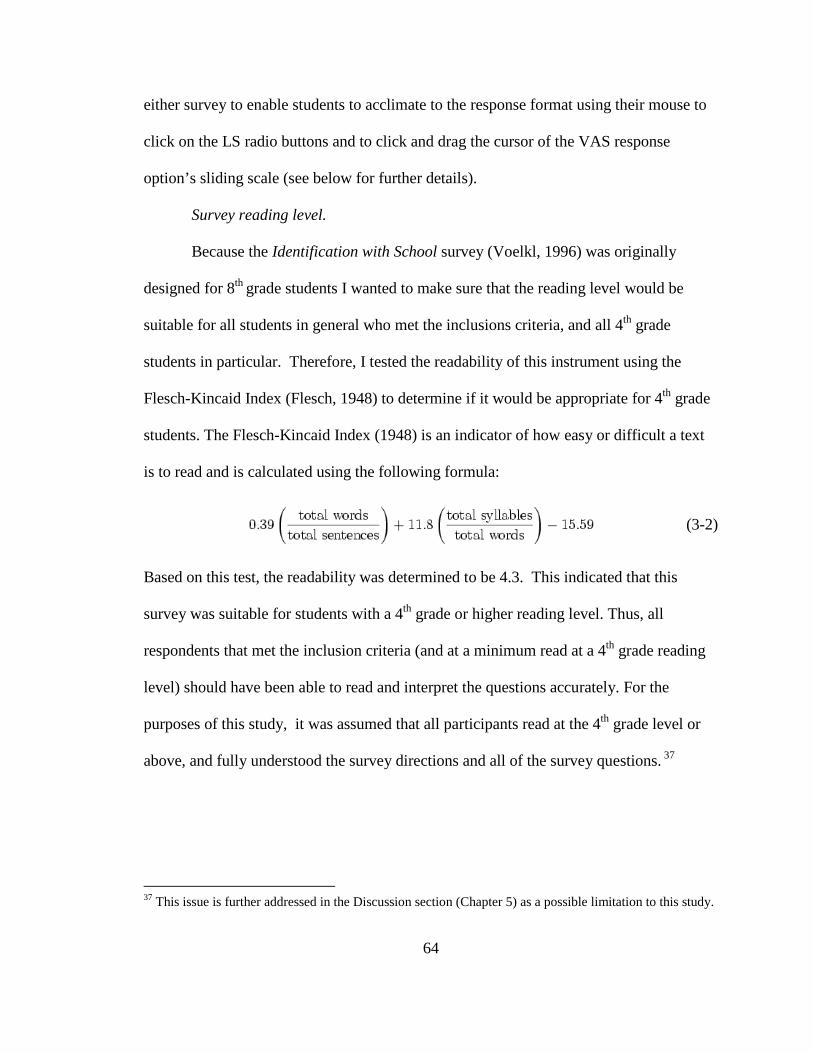
64
either survey to enable students to acclimate to the response format using their mouse to
click on the LS radio buttons and to click and drag the cursor of the VAS response
option’s sliding scale (see below for further details).
Survey reading level.
Because the Identification with School survey (Voelkl, 1996) was originally
designed for 8th grade students I wanted to make sure that the reading level would be
suitable for all students in general who met the inclusions criteria, and all 4th grade
students in particular. Therefore, I tested the readability of this instrument using the
Flesch-Kincaid Index (Flesch, 1948) to determine if it would be appropriate for 4th grade
students. The Flesch-Kincaid Index (1948) is an indicator of how easy or difficult a text
is to read and is calculated using the following formula:
(3-2)
Based on this test, the readability was determined to be 4.3. This indicated that this
survey was suitable for students with a 4th grade or higher reading level. Thus, all
respondents that met the inclusion criteria (and at a minimum read at a 4th grade reading
level) should have been able to read and interpret the questions accurately. For the
purposes of this study, it was assumed that all participants read at the 4th grade level or
above, and fully understood the survey directions and all of the survey questions. 37
37 This issue is further addressed in the Discussion section (Chapter 5) as a possible limitation to this study.
65
Web-based survey design features.
Both versions of the survey were Web-based and had the same number of items
and same prompts but with different ways for participants to respond. The LS version’s
response options were presented as radio buttons with choices ranging from Strongly
Disagree to Strongly Agree and the VAS version had a slider-type response option
presented with only the two extreme verbal cues of the LS (e.g., Strongly Disagree and
Strongly Agree) on each end of the slider (see Appendix J for an example of an LS and
VAS item). Respondents used their mouse to click anywhere on the continuum and a
marker appeared that could be manipulated (by sliding) in either direction to indicate
varying degrees of “positive” (e.g., agree) or “negative” (e.g., disagree) responses.
Given that it was not possible to control the settings in which the survey would be
administered or the type of computer monitor on which the survey would be presented to
students, pixels were used as the standard measurement for the length of the VAS line
rather than stipulating the more traditional 10cm or 100mm length established for paper-
based versions of surveys. In this way, I was able to obtain the most accurate scores
possible without having had to administer the survey with a standardized computer and
monitor across all settings and conditions.
Supplemental post-survey questionnaire.
Subsequent to completing the Identification with School survey, all respondents
were asked three additional web-based, open-response questions to assess their
immediate reaction to the survey and to the two response formats used (see Appendix C).
The readability of these post-survey questions was tested using the Flesch-Kincaid Index
66
(Flesch, 1948) to determine if they were appropriate for participants with at least a 4th
grade reading level. Upon completion of this test, the readability was determined to be
4.6, which indicated that this questionnaire was suitable for students with a 4th grade or
higher reading level. Thus, all respondents that met the inclusion criteria (and at a
minimum read at a 4th grade reading level) should have been able to read and interpret
these questions accurately.
Student demographic questionnaire.
A six-item demographic questionnaire (see Appendix D) was administered after
participants took the LS and VAS surveys and the post-survey questionnaire (see
Appendices A, B, and C). A Flesch-Kincaid (1948) analysis of the readability of this
questionnaire suggested that the reading level was 4.2. Thus, all respondents that met the
inclusion criteria (and at a minimum read at a 4th grade reading level) should have been
able to read and interpret these questions accurately as well.
Scoring Criteria
Because the LS and VAS response options were qualitatively different, it was
necessary to develop scoring criteria that would allow comparisons of the two response
formats. Below is a description of how each version was scored.
Scoring the Likert scale version.
To respond using the Likert scale, participants were required to use their mouse to
click on a radio button that corresponded with their desired response (e.g. Strongly
Disagree to Strongly Agree). The LS items were scored as follows: Strongly Disagree =
67
1, Disagree = 33, Agree = 66, and Strongly Agree = 99. The 16-items in the Identification
with School survey were summed to create an “identification with school” score for each
participant, with a possible range of summated scores of 16-1584. This scoring method
was selected in an effort to closely match that of the VAS, which is explained in further
detail in the next section. Lastly, it was assumed that low identification with school
was an undesired personal attribute. Therefore, all items that reflected a negative
identification with school (e.g., a high score indicated a low sense of belongingness or of
valuing school and school-related outcomes) were re-coded so that higher values on all
16 items indicated a higher identification with school. After examining the wording of
each item and confirming that negatively-worded items had a negative correlation with
other items in the inter-item correlation matrix, it was decided that items 3, 4, 7, 8, 9, and
14 needed to be recoded (see Appendix A). For the LS version, student responses for
these six items were recoded as follows: 99 = 1; 66 = 33; 33 = 66; and 1 = 99.
Scoring the VAS version.
To respond using the VAS, participants were asked to select a place along the
continuum between Strongly Disagree and Strongly Agree that best matched how they
felt in response to the presented item prompt. Participants indicated their perceived status
for each of the 16 items by using their mouse to click on each 99-pixel horizontal line (or
continuum) at a point that was personally “most appropriate” (Flynn, van Schaik, & van
Wersch, 2004, p.50). The positions of each respondent’s “clicks” or “marks” on the VAS
line were scaled as one of 99 distinct points, resulting in score points from a possible
range of 1-99 for each item (e.g., each of the VAS line’s 99 pixels was a score point).
68
Thus, as with the LS version, the possible range of summated scores for the 16-item VAS
survey was 16-1584—with a higher summated score indicating a higher level of a
student’s identification with school—and items 3, 4, 7, 8, 9, and 14 were recoded because
they reflected a negative identification with school (see Appendix B). To recode items 3,
4, 7, 8, 9, and 14 for the VAS, responses were subtracted from 100 and the differences
replaced the old values so that higher values indicated a higher identification with school.
Research Questions
This study attempted to address the following research questions:
1. Does the response format change the factor structure of the survey?
2. Does the response format affect the reliability coefficient?
3. Are there significant mean differences for the summated scores overall between the LS version and the VAS version of the survey?
4. Are there significant mean differences of the summated scores on the LS and VAS versions of the survey between Elementary, Middle, and High School students?
5. Is there a significant interaction between level of schooling and item response type? If so, is it dependent on item response type?
Statistical Analyses
Data Analysis
Using the SPSS statistical package (version 14.0), variables were tested for
violation of the normality distribution assumptions for the use of parametric statistics. All
69
variables were checked for skewness and kurtosis ratios to ensure they are within the
limit of three. As mentioned above, this study sought to contribute to the literature in K-
12 educational survey research by comparing a previously validated survey originally
comprising items with LS response options to an equivalent survey with visual analog-
scaled (VAS) response options. To do so, this study examined each response format’s
affect on four indices: factor structure, reliability, summated mean scale scores, and
simple-, main-, and interaction effects.
Index 1: Factor Structure
Factor structure was examined to determine whether items in the Identification
with School survey measured a “single, common phenomenon” (McIver & Carmines,
1981) and if the survey’s unidimensionality differed as a function of item response type.
In other words, each version of the survey was examined to determine if altering the
survey’s response options from the LS to the VAS resulted in equivalent factor structures.
To examine the factor structure of the Identification with School survey, correlation
matrices were factor analyzed using principal components analyses with Varimax
rotation. Multiple criteria were used to decide the optimal number of components to
retain.
Principal components analysis.
A principal components analysis (PCA) was conducted for the LS and VAS
versions of the Identification with School survey to determine if the underlying factor
structure was consistent between the two item response formats. The underlying objective
70
in PCA is to obtain orthogonal linear combinations of the original variables in a data set
that account for as much of the total variance in the original variables as possible
(Tabachnick & Fidell, 2001). Put simply, PCA groups highly correlated items together
with the assumption that they were influenced by the same underlying dimension
(component). One goal of conducting PCA in this study was to extract from the data a
reduced set of uncorrelated components that accounted for most of the variance in the
original set of variables. Although factor structure (i.e. determining the number of
components) was of primary interest, a secondary goal was to summarize the pattern of
intercorrelations among the items on the Identification with School survey.
Typically, the most critical problem a researcher faces when conducting a PCA is
determining the number of components to retain (Hayton, Allen, & Scarpello, 2004;
Velicer, Eaton, & Fava, 2000; Zwick & Velicer, 1986). Specifying too few (e.g., under-
extraction) can lead to a loss of information and/or distorted38 component loadings, and
specifying too many (e.g., over-extraction) can lead to the inclusion of minor or “false”
components in the model that can obfuscate interpretation and detract from the major or
“true” components (Fabrigar, Wegener, MacCallum, & Strahan, 1999; Zwick & Velicer,
1986). Because of these pivotal consequences, multiple criteria were employed in this
study to determine the optimal number of components to retain for each version of the
survey. Although the Kaiser rule or the “eigenvalue greater than one” rule (K1) is one of
the most popular methods (Velicer, Eaton, & Fava, 2000) for determining the number of
38 Distorted component loadings due to underextraction can result when a researcher ignores the presence of a major component or when a component is conflated with another thus resulting in a loss of important information.
71
components to retain when conducting a PCA , it was not used in this study primarily due
to the large body of literature that recommends K1 not be used because it tends to yield
inaccurate results (Cattell & Vogelmann, 1977; Cliff, 1988; Fabrigar, Wegener,
MacCallum, & Strahan, 1999; Gorsuch, 1983; Hayton, Allen, & Scarpello, 2004;
Schomemann, 1990; Velicer, Eaton, & Fava, 2000). Specifically, K1 has been shown to
consistently overestimate the number of components to retain (Horn, 1965; Linn, 1968;
Zwick & Velicer, 1986).
The first criterion employed to determine the number of components to retain in
the present study was Catell’s (1966) scree test, which is based on a visual inspection of a
graph of eigenvalues for significant breaks or discontinuities. Catell’s rationale for this
approach was that only “major” components account for a sizeable portion of variance
and thus have sizeable eigenvalues. As a result, when eigenvalues are plotted a distinct
break or “cliff” emerges such that major components’ eigenvalues appear higher in the
plot and the remaining, increasingly smaller eigenvalues of lesser or “minor” components
appear as “scree” or rubble at the bottom of a cliff. Once this break is identified, only
those components that are above the scree in the plot are retained. This method was
selected because it is easily applied and because it has been recommended as a useful
procedure when used in conjunction with other criteria to determine the number of
components to extract and retain (Fabrigar, Wegener, MacCallum, & Strahan, 1999;
Velicer, Eaton, & Fava, 2000).
The second criterion involved the interpretation of component loadings and was
used to validate the number of components yielded from the scree test and also helped to
72
ensure that only those components that would be considered “major” would be retained
(Guadagnoli & Velicer, 1988; Norusis, 2005). With PCA, component loadings
represent the correlation between each variable and the extracted component (which itself
represents a linear combination of the set of variables). According to Stevens (2002), too
often investigators blindly employ the rule-of-thumb of only interpreting |.30| or greater
components loadings without taking sample size into account, which is known to affect
statistical significance. He further noted that the use of the basic standard error formula
that has been traditionally used to determine a correlation coefficient’s significance
(1/ 1N − ) was far too likely to capitalize on chance when used with the PCA method
and thus result in component loading standard errors that were “seriously
underestimate[d]” (2002, p. 393). Thus, in accordance with the recommendations of
Stevens (2002), to account for the possibility of underestimated component loading
standard errors and to yield an acceptable estimate of whether component loadings were
statistically significant, I doubled the standard error used to calculate statistical
significance. To do this, I doubled the critical value required for an ordinary correlation
to achieve statistical significance for a sample of 269 participants (r = .163) and then
tested each component loading at r = |.33| (df = 267, / 2α = .01) to reduce the probability
of at least one false rejection (Stevens, 2002).
As an indicator of whether a component was “major” and thus retained for the
final model, it had to have at least four substantial or high factor loadings (Guadagnoli &
Velicer, 1988; MacCallum, Widaman, Zhang, & Hong, 1999; Norusis, 2005; Velicer &
Fava, 1998; Zwick & Velicer, 1986). A high factor loading was defined as one that was

73
|.60| or above. This definition is consistent with the recommendations of Hair, Anderson,
Tatham, and Black (1998), who maintained that loadings at or above |.60| can be
interpreted as "high" and therefore provide a very good basis for component
interpretation. Thus, for the purposes of this study, component loading values had to be at
least |.33| to be considered statistically significant and components had to have at least
four component loadings of |.60| or above to be considered “major” and thus be retained
for the final model.
The third and final criterion employed to verify that the optimal number of
components had been retained was Horn’s (1965) parallel analysis procedure. Parallel
analysis has been cited as one of the most effective methods for researchers to use to
empirically determine the number of factors or components to retain (Lance, Butts, &
Michels, 2006; O’Connor, 2000; Velicer, Eaton, & Fava, 2000; Zwick & Velicer, 1986).
Horn (1965) introduced this method of component selection as an alternative to Kaiser’s
“eigenvalue greater than one” (K1) rule. Zwick and Velicer (1986) referred to parallel
analysis as a “sample-based adaptation of the population-based K1 rule” (p. 434). Their
rationale was that sampling variability will produce eigenvalues greater than one even if
all eigenvalues of a correlation matrix are exactly one and no major components exist (as
would occur with independent variates) (Zwick & Velicer, 1986). Therefore, if the
eigenvalues of a correlation matrix generated from an actual study’s data set are
compared with the eigenvalues of a correlation matrix generated from a simulated data
set (of the same dimensions comprising only random numbers), then it can be assumed
that the “actual” (or observed) eigenvalues of major components should be larger than
74
their “simulated” eigenvalue counterparts. In short, parallel analysis enables an
investigator to extract only major components and to ignore “minor” components that
account for less variance than could be obtained from random data (O’Connor, 2000).
With parallel analysis, the traditional eigenvalue threshold of +1 is replaced with
mean eigenvalues generated from a simulated set of random data correlation matrices that
mirrors the observed data correlation matrices in the number of variables and
participants. For example, the present study’s data set comprised 269 observations for
each of the 16 variables on the Identification with School survey. Thus, a series of
simulated or parallel random data matrices of the same size (269 x 16) was generated and
eigenvalues were computed for both the observed data set’s correlation matrices and for
each of the parallel data set’s correlation matrices. The number of generated parallel data
sets is pre-determined by the investigator (although there is technically no limit to the
number that can be generated, the program used for this study maxed out at 9,999). With
each new simulated data set, a correlation matrix is generated, a PCA is conducted, and
eigenvalues are calculated until the specified maximum number is reached and then, as
Hayton, Allen, and Scarpello (2004) describe,
the average eigenvalues from the random [parallel] correlation matrices
are…compared to the eigenvalues from the real data correlation matrix, such that
the first observed eigenvalue is compared to the first random eigenvalue, the
second observed eigenvalue is compared to the second random eigenvalue, and so
on. Factors corresponding to actual eigenvalues that are greater than the parallel
average random eigenvalues should be retained. Actual eigenvalues less than or
equal to the parallel average random eigenvalues are considered due to sampling
error (p.194).
75
Once the investigator determines (from the generated output) that an observed eigenvalue
is smaller than its parallel counterpart, the procedure is stopped and the researcher retains
only the observed components that had eigenvalues larger than the simulated eigenvalues.
Although the parallel analysis is not currently available in SPSS or SAS, programs are
available to implement this method in both of these statistical programs (O' Connor,
2000; 2008). These programs can be downloaded for free at
http://people.ok.ubc.ca/brioconn/nfactors/nfactors.html
Index 2: Reliability
Reliability is the extent to which a score or measure is free of measurement error;
therefore, the lower the amount of measurement error, the higher the value for reliability.
Crocker and Algina (1986) caution that when interpreting this index, it is important to
keep in mind that “…this estimate implies nothing about the stability of the [survey]
scores over time or their equivalence to scores on one particular alternate form of the
[survey]” (p. 142). Norusis (2005) further cautions that “the reliability of a scale depends
on the population to which it is administered. Different populations of subjects may result
in different scale properties” (p.428).
Although the meaning of a reliability coefficient will vary as a function of the
type of characteristic measured and the method of obtaining the estimate(s) of reliability,
there are several ways of interpreting a reliability coefficient of a given value. One
method is to interpret a reliability coefficient as the proportion of observed score variance
that is “true” rather than “error” variance. For example, a reliability coefficient of .749
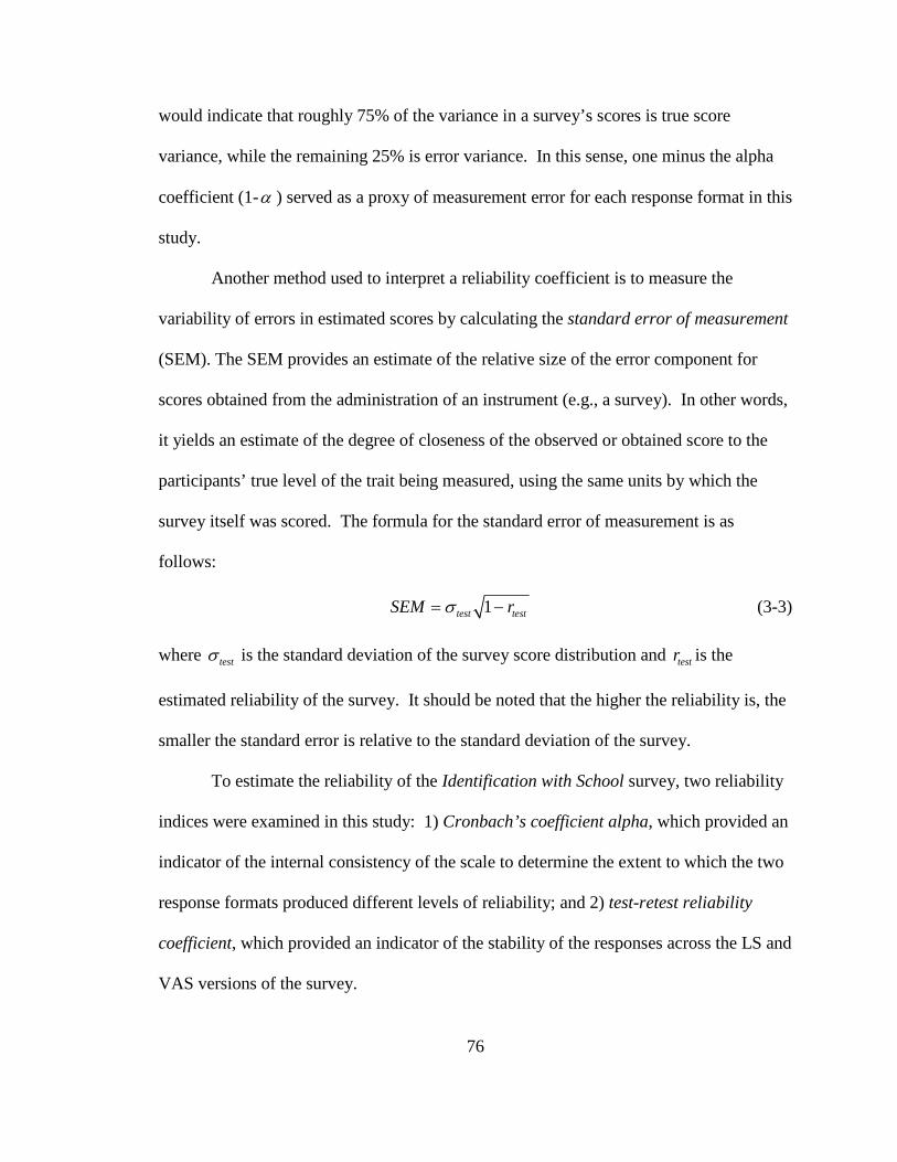
76
would indicate that roughly 75% of the variance in a survey’s scores is true score
variance, while the remaining 25% is error variance. In this sense, one minus the alpha
coefficient (1-α ) served as a proxy of measurement error for each response format in this
study.
Another method used to interpret a reliability coefficient is to measure the
variability of errors in estimated scores by calculating the standard error of measurement
(SEM). The SEM provides an estimate of the relative size of the error component for
scores obtained from the administration of an instrument (e.g., a survey). In other words,
it yields an estimate of the degree of closeness of the observed or obtained score to the
participants’ true level of the trait being measured, using the same units by which the
survey itself was scored. The formula for the standard error of measurement is as
follows:
1test testSEM rσ= − (3-3)
where testσ is the standard deviation of the survey score distribution and testr is the
estimated reliability of the survey. It should be noted that the higher the reliability is, the
smaller the standard error is relative to the standard deviation of the survey.
To estimate the reliability of the Identification with School survey, two reliability
indices were examined in this study: 1) Cronbach’s coefficient alpha, which provided an
indicator of the internal consistency of the scale to determine the extent to which the two
response formats produced different levels of reliability; and 2) test-retest reliability
coefficient, which provided an indicator of the stability of the responses across the LS and
VAS versions of the survey.

77
Cronbach’s alpha.
Cronbach’s alpha (α ) is a measure of internal consistency directly affected by
the number of items, the variability in the item responses, and the magnitude of the
intercorrelation between items. Although there are other ways to measure internal
consistency besides Cronbach’s alpha, each of which begins with different assumptions
and uses different analytic approaches in studying relationships between the items,
evidence suggests that they all arrive at virtually the same estimates of reliability
(Pedhazur & Pedhazur-Schmelkin, 1991). In view of this, Cronbach’s alpha was selected
due to its popular use and familiarity in the educational research literature.
Test-retest reliability.
Test-retest reliability (rxx′) is often referred to as a coefficient of stability and
depending on the type of data being analyzed, the researcher will either apply Pearson r
or Spearman rho to the total scores of the two tests or surveys that were administered.
For the purposes of this study, I assumed that the LS and VAS response options yielded
interval-level data. As such, I used the Pearson product-moment correlation coefficient to
examine the linear relationship or correlation between the scores on the administrations
of the two forms of the survey, with a high correlation indicating high test-retest
reliability, thus suggesting that the responses across both administrations were stable.
Lastly, to obtain an estimate of random error, I subtracted the resultant correlation from 1
(e.g., 1 - r).

78
Index 3: Summated Mean Scale Scores
Summated mean scale scores were evaluated to determine whether the LS and
VAS response formats produce significantly different summated scale score means, in
general, and different means for the students, in particular. The LS items were scored as
follows: Strongly Disagree = 1, Disagree = 33, Agree = 66, and Strongly Agree = 99.
The 16-items in the Identification with School survey were summed to create an
“identification with school” score for each participant, with a possible range of summated
scores of 16-1584. To score the VAS items, the positions of each respondent’s “clicks” or
“marks” on the VAS line were scaled as one of 99 distinct points, resulting in score
points from a possible range of 1-99 for each item (e.g., each of the VAS line’s 99 pixels
was a score point). As with the LS version, the possible range of summated scores for the
16-item VAS survey was 16-1584, with a higher summated score indicating a higher
level of a student’s identification with school.
Index 4: Simple-, Main-, and Interaction Effects
Chronological age has been shown in previous studies to be a significant factor in
children’s performance on surveys due to developmental factors that can impact
cognitive abilities involving spatial reasoning or understanding and manipulating ordinal
relations (Cremeens, Eiser, & Blades, 2007; Read & MacFarlane, 2006; Shields, Cohen,
Harbeck-Weber, Powers, & Smith, 2003; van Laerhoven, van der Zaag-Loonen, &
Derkx, 2004); therefore, in this study the effects of age and item type were examined in
an effort to determine if there were any significant differences between how younger
79
students and older students responded when presented with VAS vs. LS response options.
Consequently, simple-, main-, and interaction effects focused on the differences among
group means to determine if manipulating the response-type variable yielded significant
effects.
Simple effects are comparisons of differences between means for the levels of one
independent variable (IV) within the levels of a second IV, and main effects are
differences on the dependent variable (DV) attributed to an IV (Keppel & Wickens,
2004). Put another way, a main effect is the effect of an IV uninfluenced by other
variables. Interaction effects, are an indication that the effect of the levels of one IV is not
the same across the levels of a second IV (2004). When examining simple effects, it is
important to remember to adjust the reported significance levels in accordance with the
level of heterogeneity of variances of score deviations from group means in order to keep
the Type I error rate below the 5 percent threshold (Klockars & Sax, 1986). According to
Keppel and Wickens (2004), if there are large deviations of scores from the mean/median
within each group and heterogeneous differences in variances across groups, reducing
the level to roughly half (e.g., =.025) would be appropriate because this reduction would
“…[bring] the actual Type I error rate back to where it belongs [e.g., =.05]” (p.153).
Nonetheless, one must be careful if the variances do not differ at all or differ only a little
because reducing alpha reduces power, which could result in the rejection of a true null
(Type I error). To measure simple, main, and interaction effects, a factorial ANOVA was
conducted.
80
Factorial ANOVA.
The advantage of a randomized, 2x3 between-subjects experimental design is that
factorial ANOVA can be used to examine the joint effect of the two factors acting in
concert to influence the dependent variable (DV). Advantages of the factorial ANOVA
design include its efficiency, power, and the detection of interactions. Conducting a
factorial ANOVA offers a more efficient use of both the researcher’s and participants’
time because it allows for the study of the effects of two (or more) factors on the same
dependent variable with a single experiment as opposed to the two or more required for
separate one-way designs (Kerlinger, 1992). Additionally, power is increased when both
factors A and B are determinants of variance in the participants’ dependent variable
scores because factorial ANOVA tends to yield a smaller error term (denominator of the
F ratio) than would a one-way ANOVA on just one factor (1992). That is, the error
variance due to factor B and AxB is removed from the denominator of the F ratio
(MSError), which tends to increase the F for factor A (thereby increasing power). With
simultaneous analysis of the two factors, the researcher is in essence able to carry out two
separate research studies concurrently.
Steps taken to conduct the ANOVA.
In order to examine whether age/school level and/or item response type were
related to students’ summated scores on the Identification with School survey, a two-way
fixed-effects, between-groups factorial ANOVA was conducted and F ratios were
calculated for each of the following:
� The main effect of school level (Factor A)

81
� The main effect of the item response type (Factor B)
� The interaction between school level and item response type (AxB)
� The simple effects within school level (Factor A)
The following null hypotheses addressed the main effects for each factor and the
possible interaction between factors:
1. The means of the LS and VAS conditions (Factor A) are the same:
H01: 1 2A Aµ µ=
H11: 1 2A Aµ µ≠
2. The means of the different school levels (Factor B) are the same:
H02: 1 2 3B B Bµ µ µ= =
H12: 1 2 3B B Bµ µ µ≠ ≠
3. The differences between the means of the different levels of the interaction are the same:
H03: 11 21 21 22 13 32AB AB AB AB AB ABµ µ µ µ µ µ− = − = −
H13: 11 21 12 22 13 32AB AB AB AB AB ABµ µ µ µ µ µ− ≠ − ≠ −
Criterion for Rejecting H 0
The test statistic used for all three hypotheses was the F ratio and the sampling
distribution was the F distribution with appropriate degrees of freedom. The degrees of
freedom associated with the main effects, the interaction, and the within cell mean
squares are presented in Table 3-2 below.
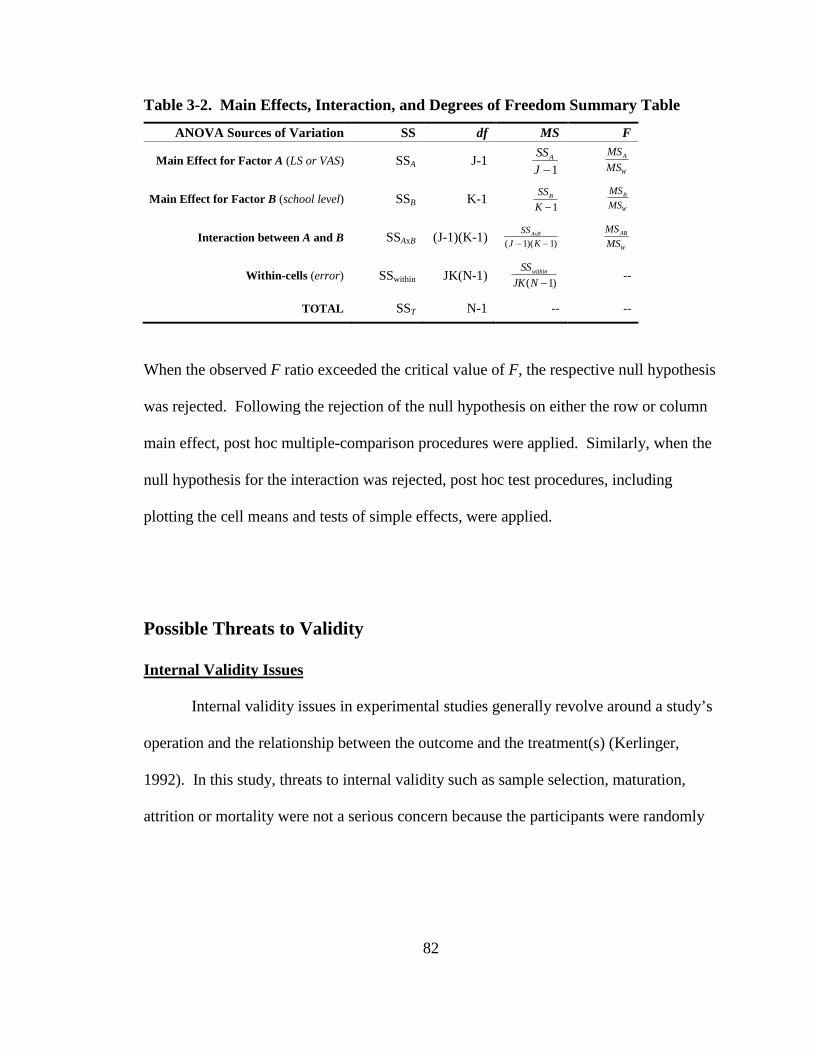
82
Table 3-2. Main Effects, Interaction, and Degrees of Freedom Summary Table
ANOVA Sources of Variation SS df MS F
Main Effect for Factor A (LS or VAS) SSA J-1 1
ASS
J − A
W
MS
MS
Main Effect for Factor B (school level) SSB K-1 1
BSS
K −
B
W
MS
MS
Interaction between A and B SSAxB (J-1)(K-1) ( 1)( 1)AxBSS
J K− −
AB
W
MS
MS
Within-cells (error) SSwithin JK(N-1) ( 1)
withinSS
JK N−
--
TOTAL SST N-1 -- --
When the observed F ratio exceeded the critical value of F, the respective null hypothesis
was rejected. Following the rejection of the null hypothesis on either the row or column
main effect, post hoc multiple-comparison procedures were applied. Similarly, when the
null hypothesis for the interaction was rejected, post hoc test procedures, including
plotting the cell means and tests of simple effects, were applied.
Possible Threats to Validity
Internal Validity Issues
Internal validity issues in experimental studies generally revolve around a study’s
operation and the relationship between the outcome and the treatment(s) (Kerlinger,
1992). In this study, threats to internal validity such as sample selection, maturation,
attrition or mortality were not a serious concern because the participants were randomly

83
assigned39 to treatment conditions and then immediately took the online survey. Further,
because the treatments were only administered during a single session rather than over
time, students neither had time to mature nor leave the study for any number of reasons.
External Validity Issues
External validity issues generally deal with populations, settings, and variables
and whether or not they can be generalized to a population. In this study, given that the
focus was on how students responded to the LS and VAS item response types rather than
on students’ responses in isolation, it is important to note that it is not the intention of the
researcher to generalize the results of the Identification with School survey beyond the
scope of this exploratory study. Therefore, the meaningfulness of the outcome of the
survey administered in this study (e.g., whether students like school or identify with
school) was not examined in detail. As such, the findings of this study as they relate to
the construct that was measured should be interpreted with caution.
39 It bears noting that even with randomization the groups could have been different due to chance.

84
Chapter 4: Results
Introduction
In this chapter, the results are organized according to the analyses performed to
answer each of the five research questions. To begin, a description of the sample is
presented. Next, results of the principal components analysis are presented, followed by
the reliability analyses of the two versions of the survey, the summated score
comparisons, and the factorial ANOVAs. Finally, the results of the post-survey
questionnaires are presented.
Sample
The online survey was accessed 455 times between May 1, 2008 and June 30,
2008. The study’s exclusion criteria—which excluded participants from the study if their
reported aged was younger than nine years old, if their reported grade was lower than
Grade 4, or if they failed to provide their age and grade—yielded 269 students for the
final analyses. Students ranged in age from 9 to 19 years (M=13.67, SD=3.07) and were
in grades 4 through 12. More than one-fourth of the participants were in Grade 12 (n=68)
and nearly one-fourth were 11-years-old (n=60). The smallest groups of students by
grade and age were grade 7 (n=3) and ages 9 and 13 (n=9 for both). There was a slightly
greater percentage of girls than boys in the sample (48.3% vs. 45.0%) and nearly 75% of
the students were native English speakers. Table 4-1 presents detailed demographic data
for the sample used for this study.
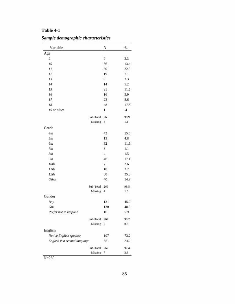
85
Table 4-1
Sample demographic characteristics
Variable N % Age 9 9 3.3
10 36 13.4 11 60 22.3 12 19 7.1 13 9 3.3
14 14 5.2 15 31 11.5 16 16 5.9 17 23 8.6
18 48 17.8 19 or older 1 .4
Sub-Total 266 98.9
Missing 3 1.1
Grade 4th 42 15.6
5th 13 4.8 6th 32 11.9 7th 3 1.1 8th 4 1.5
9th 46 17.1 10th 7 2.6 11th 10 3.7 12th 68 25.3 Other 40 14.9
Sub-Total 265 98.5
Missing 4 1.5
Gender Boy 121 45.0 Girl 130 48.3 Prefer not to respond 16 5.9
Sub-Total 267 99.2
Missing 2 0.8
English Native English speaker 197 73.2 English is a second language 65 24.2
Sub-Total 262 97.4
Missing 7 2.6
N=269
86
Of the 40 students who selected “Other” as their grade-level, 95% (n=38) were the same
age as students in the Upper Elementary (Grades 4-6) school level. The remaining 5%
(n=2) were the same age as students in the Middle school level. Because summated
scores for the students in the Other group were similar to those of their same-aged peers
on the LS and VAS versions of the surveys, these students were “re-assigned” into the
school-level group that best matched their reported age. Similarly, there were four
students who reported only age and not grade and they were subsequently merged into
their respective school-level peers’ group. Results in all subsequent tables include these
school-level reassignments.
Categorical Variables
To address the potential biasing effects of students being “misclassified” into the
incorrect age/developmental level group or grade/school level group, the age and grade
variables were dummy coded so that analyses could be conducted based solely on
reported ages or on reported grades for comparison purposes. For the Age groups
variable, participants were classified according to one of three categories: 1) Later
Childhood, 9 to 12 years-old; 2) Early Adolescence, 13 to15 years-old; or 3) Later
Adolescence, 16 to18 years-old. For the School-Level groups variable, participants were
classified according to one of three categories: 1) Upper Elementary, 4th to 6th grade; 2)
Middle, 7th to 9th grade; or 3) High School, 10th to 12th grade. Table 4-2 presents the
number and percentages of students within each group. For the remainder of this chapter,
only the results of the School-Level groups are reported because no significant

87
differences between the School-Level and Age groups were found in subsequent analyses
of reliability coefficients or summated scores on either version of the Identification with
School survey.
Table 4-2.
Grouping Variables by School-Level and Age
Variable n %
School-Level groups
Upper Elementary (grades 4-6) 126 46.8
Middle School (grades 7-9) 58 21.6
High School (grades 10-12) 85 31.6
Total: 269 100.0
Age groups
Later Childhood (ages 9-12) 124 46.1
Early Adolescence (ages 13-15) 54 20.1
Later Adolescence (ages 16-18) 87 32.3
Sub-Total: 265 98.5
Missing: 4 1.5
N = 269
Experimental Conditions
As described in Chapter 3, students in grades four through twelve were blocked or
grouped by school level as they entered the system and then randomly assigned to one of
the two different conditions. Students assigned to Condition One (n = 146, 54.3%) were
administered the LS version of the survey first followed by the VAS version and students
in Condition Two (n = 123, 45.7%) were administered the VAS version of the survey
first followed by the LS version. Although a randomization program kept participant
levels of both conditions approximately balanced overall, there were 23 more students in
88
Condition One than in Condition Two after deletions due to exclusion criteria. No
significant differences emerged between the two conditions in subsequent analyses (e.g., t
tests of summated scores and reliability coefficients) thereby demonstrating no order
effects.
Factor Structure
Research question #1
Does the response format change the factor structure of the survey?
Principal Components Analysis
To determine the appropriateness of factoring the LS and VAS correlation
matrices, the Kaiser-Meyer-Olkin (KMO) overall measure of sampling adequacy40 was
conducted, which yielded .83 and .85 for the LS and VAS versions, respectively. The
KMO measure varies between 0 and 1 and values closer to 1 are desirable. Kaiser (1974)
categorized KMO measures in the 0.80’s as “meritorious” and anything below 0.50 as
unacceptable. Norusis (2005) suggested that KMO values above .60 (“mediocre” in
Kaiser’s terms) indicate a factorable correlation matrix with linearly related items, which
in turn indicates that it is reasonable for the investigator to proceed with the principal
components analysis (PCA). As such, the results from the present study for the KMO
40 It bears noting that Bartlett’s Test of Sphericity was not conducted due to its notorious sensitivity to sample size. Tabachnick and Fidell (2001) suggest that this test only be used with smaller samples where n ≤ 5 participants per variable.

89
exceed this threshold indicating that the sample size of N=269 was sufficient for PCA
and that both the LS and VAS matrices were highly factorable.
Scree Test
A PCA with Varimax rotation was conducted to determine the underlying
variance structure for measures on the 16 items comprising both the LS and VAS
versions of the Identification with School survey. The orthogonal Varimax rotation
method was selected because it minimizes factor complexity by maximizing variance for
each factor (Tabachnick & Fidell, 2001). Following a visual inspection of scree plots (see
Figure 4-1 below), the initial PCA solutions suggested a single component for both the
LS and VAS according to Catell’s (1966) criteria for component extraction.
Figure 4-1. Scree plots of LS vs. VAS initial solutions.
Component Loadings Assessment
In her final assessment of the factor structure of the Identification with School
survey, Voelkl (1996) presented evidence that suggested her scale was unidimensional;
however, prior to coming to this conclusion she tested a two-factor solution comprising
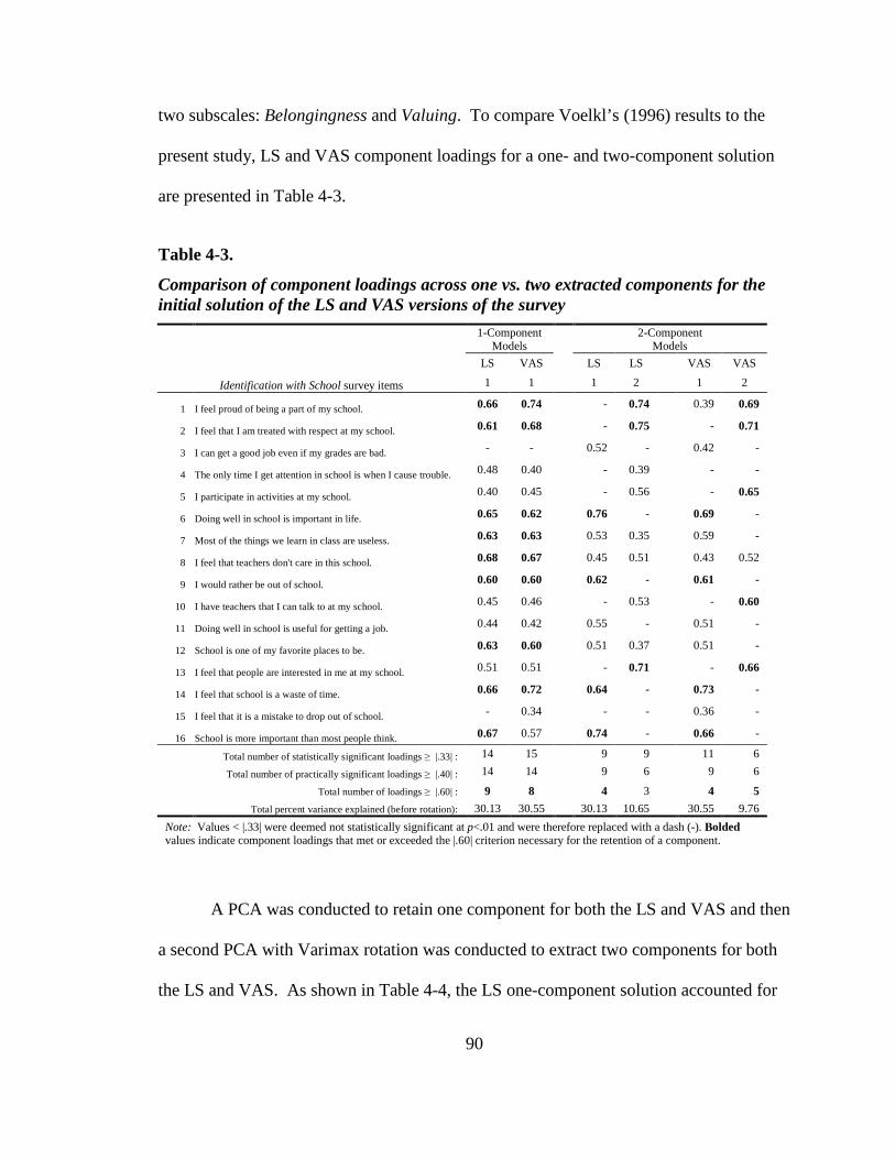
90
two subscales: Belongingness and Valuing. To compare Voelkl’s (1996) results to the
present study, LS and VAS component loadings for a one- and two-component solution
are presented in Table 4-3.
Table 4-3.
Comparison of component loadings across one vs. two extracted components for the initial solution of the LS and VAS versions of the survey
1-Component
Models 2-Component Models
LS VAS LS LS VAS VAS
Identification with School survey items 1 1 1 2 1 2
1 I feel proud of being a part of my school. 0.66 0.74 - 0.74 0.39 0.69
2 I feel that I am treated with respect at my school. 0.61 0.68 - 0.75 - 0.71
3 I can get a good job even if my grades are bad. - - 0.52 - 0.42 -
4 The only time I get attention in school is when I cause trouble. 0.48 0.40 - 0.39 - -
5 I participate in activities at my school. 0.40 0.45 - 0.56 - 0.65
6 Doing well in school is important in life. 0.65 0.62 0.76 - 0.69 -
7 Most of the things we learn in class are useless. 0.63 0.63 0.53 0.35 0.59 -
8 I feel that teachers don't care in this school. 0.68 0.67 0.45 0.51 0.43 0.52
9 I would rather be out of school. 0.60 0.60 0.62 - 0.61 -
10 I have teachers that I can talk to at my school. 0.45 0.46 - 0.53 - 0.60
11 Doing well in school is useful for getting a job. 0.44 0.42 0.55 - 0.51 -
12 School is one of my favorite places to be. 0.63 0.60 0.51 0.37 0.51 -
13 I feel that people are interested in me at my school. 0.51 0.51 - 0.71 - 0.66
14 I feel that school is a waste of time. 0.66 0.72 0.64 - 0.73 -
15 I feel that it is a mistake to drop out of school. - 0.34 - - 0.36 -
16 School is more important than most people think. 0.67 0.57 0.74 - 0.66 -
Total number of statistically significant loadings ≥ |.33| : 14 15 9 9 11 6
Total number of practically significant loadings ≥ |.40| : 14 14 9 6 9 6
Total number of loadings ≥ |.60| : 9 8 4 3 4 5
Total percent variance explained (before rotation): 30.13 30.55 30.13 10.65 30.55 9.76
Note: Values < |.33| were deemed not statistically significant at p<.01 and were therefore replaced with a dash (-). Bolded values indicate component loadings that met or exceeded the |.60| criterion necessary for the retention of a component.
A PCA was conducted to retain one component for both the LS and VAS and then
a second PCA with Varimax rotation was conducted to extract two components for both
the LS and VAS. As shown in Table 4-4, the LS one-component solution accounted for
91
30.13% of the variance and the VAS one-component solution accounted for 30.55% of
the variance. For the LS two-component solution (before rotation), the first component
accounted for 30.13% of the variance and the second component accounted for 10.65%
for a total of 40.78% of the variance accounted for by the two components. For the VAS
two-component solution (before rotation), the first component accounted for 30.55% and
the second component accounted for 9.76% for a total of 40.31% of the variance
accounted for by the two extracted components.
Using the second criterion for extraction (see Chapter 3), each component loading
from the rotated component matrices was tested for statistical significance at |.33|
(N=269; α = .01, two-tailed test) to reduce the probability of at least one false rejection
in accordance with the recommendations of Stevens (2002, p. 394). As an indicator of
whether a component was practically significant or “major” and thus retained for the
final model, it had to have at least four substantial or high factor loadings (Guadagnoli &
Velicer, 1988; MacCallum, Widaman, Zhang, & Hong, 1999; Norusis, 2005; Velicer &
Fava, 1998; Zwick & Velicer, 1986). A high factor loading was defined as one that was
|.60| or above.
The observed pattern of component loadings presented in Table 4-4 confirms the
findings of the scree tests presented above and suggests that, as Voelkl (1996) concluded,
a single-component model would work just as well as a two-component model for the
Identification with School survey. First, not much was gained by extracting the second
component for either the LS or VAS as the amount of variance accounted for was only
increased roughly 10%. Second, the LS two-component model did not satisfy the second

92
criterion for retention as the second extracted component only had three component
loadings ≥ |.60| and thus was rejected. Although the VAS two-component model met the
second criterion, the factor loadings did not increase substantially over those from the
one-component solution. Moreover, the interpretability of the two-component solution
was equivocal with notable cross-loading (significant component loadings on more than
one component) between the first and second components on survey items #1 and #8.
The one noteworthy advantage that the VAS two-component model had over the one-
component model was the practically significant .42 component loading on survey item
#3. For the VAS one-component model, the component loading for item #3 was not
statistically significant. Lastly, the total number of component loadings ≥ |.60| for the LS
one-component model was higher than for the two-component model (9 vs. 7,
respectively) and the total number for the VAS one- and two-component models were
nearly the same (8 vs. 9, respectively).
Based on the evidence presented in Table 4-4, the observed pattern of loadings
suggests that retaining a second component for either version of the survey does not
appear to be warranted. Additionally, the results presented confirm Voelkl’s (1996)
unidimensional or single factor structure for both the LS and VAS versions of the
Identification with School survey.
Parallel Analysis Procedure
The third and final criterion employed to determine the number of components to
retain was Horn’s (1965) parallel analysis procedure. The SPSS program written by
93
O’Connor (2000, 2008) for the parallel analysis procedure was used to simulate random
data correlation matrices that equaled the observed data correlation matrices in the
number of variables and participants (see Appendix K for the SPSS syntax used to
generate the output in Figures 4-2 and 4-3). The eigenvalues of the correlation matrices
generated from the simulated data set were averaged and then compared to the
eigenvalues of the correlation matrix generated using this study’s observed data. The
comparison of simulated- and observed-data correlation matrices is motivated by Horn’s
(1965) contention that if extracted components are to be considered “major,” (or of major
importance to explaining variance) the observed eigenvalues should be larger than their
simulated eigenvalue counterparts. Otherwise, the investigator risks retaining “minor”
components that account for less variance than could be obtained from random data
(O’Connor, 2000).
Figure 4-2 presents a side-by-side comparison of the observed LS data
eigenvalues vs. simulated eigenvalues. For the LS data it was necessary to generate the
maximum number of 9,999 random data sets to clearly differentiate between the observed
and simulated eigenvalues. This was done in accordance with O’Connor (2000), who
maintained that if the observed and simulated eigenvalues are similar in magnitude the
program should be run again using more simulated data sets until a clear difference
emerges to ensure more accurate and reliable results. Looking at Figure 4-2, it is apparent
that only the first two observed eigenvalues are larger than the corresponding first two
mean and 95th percentile random data eigenvalues. However, it bears noting the
substantial difference between the first observed data eigenvalue and its simulated
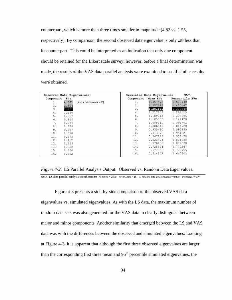
94
counterpart, which is more than three times smaller in magnitude (4.82 vs. 1.55,
respectively). By comparison, the second observed data eigenvalue is only .28 less than
its counterpart. This could be interpreted as an indication that only one component
should be retained for the Likert scale survey; however, before a final determination was
made, the results of the VAS data parallel analysis were examined to see if similar results
were obtained.
Figure 4-2. LS Parallel Analysis Output: Observed vs. Random Data Eigenvalues.
Note. LS data parallel analysis specifications: N cases = 253; N variables = 16; N random data sets generated = 9,999; Percentile = 95th
Figure 4-3 presents a side-by-side comparison of the observed VAS data
eigenvalues vs. simulated eigenvalues. As with the LS data, the maximum number of
random data sets was also generated for the VAS data to clearly distinguish between
major and minor components. Another similarity that emerged between the LS and VAS
data was with the differences between the observed and simulated eigenvalues. Looking
at Figure 4-3, it is apparent that although the first three observed eigenvalues are larger
than the corresponding first three mean and 95th percentile simulated eigenvalues, the
Simulated Data Eigenvalues: 95th Component Mean EVs Percentile EVs 1. 1.457475 1.553440 2. 1.357298 1.425147 3. 1.281681 1.337648 4. 1.217632 1.268119 5. 1.159213 1.204096 6. 1.105303 1.147428 7. 1.055311 1.096702 8. 1.006619 1.044720 9. 0.959410 0.996980 10. 0.913371 0.951821 11. 0.867883 0.907178 12. 0.822404 0.861938 13. 0.776430 0.817230 14. 0.728358 0.770267 15. 0.677066 0.722755 16. 0.614547 0.667603
Observed Data Eigenvalues: Component EVs 1. 4.821 [# of components = 2] 2. 1.704 3. 1.261 4. 1.160 5. 0.957 6. 0.918 7. 0.744 8. 0.698 9. 0.627 10. 0.610 11. 0.573 12. 0.462 13. 0.425 14. 0.390 15. 0.350 16. 0.302
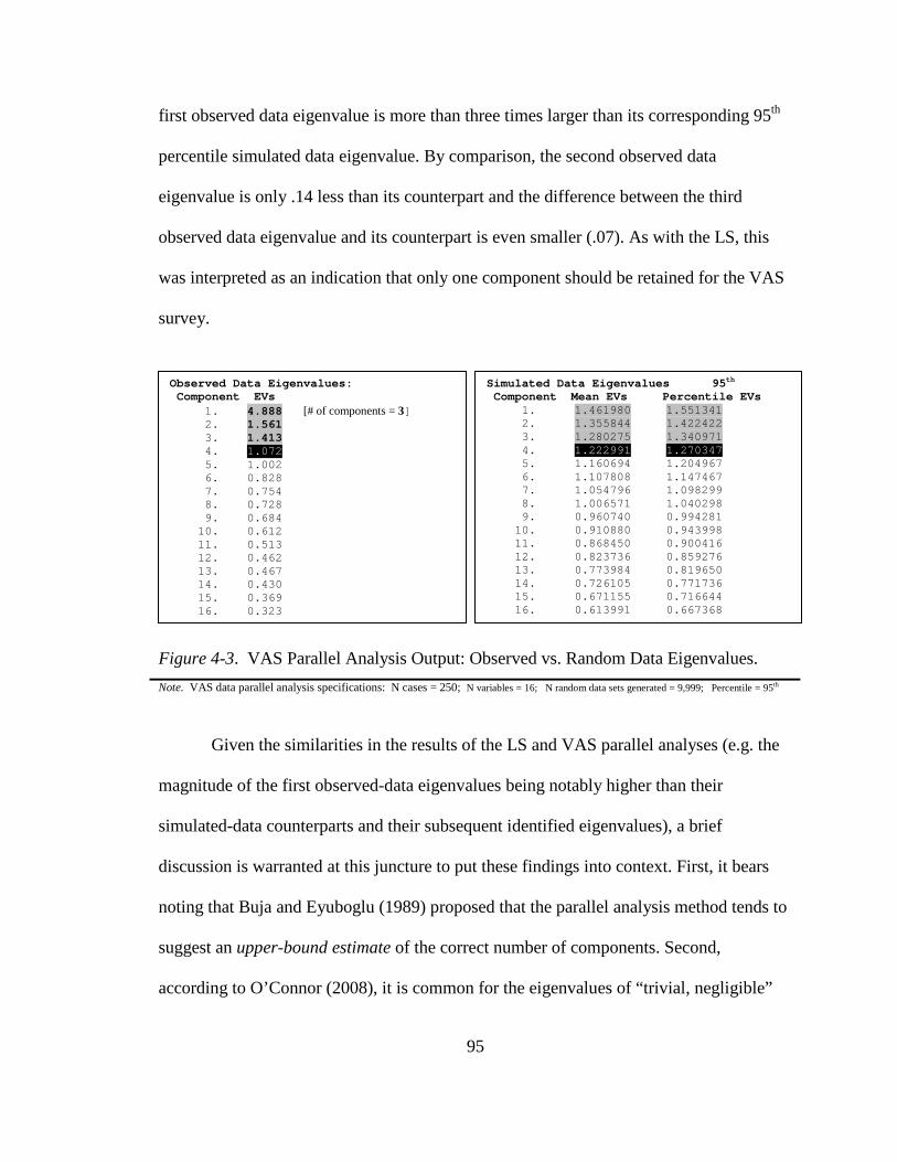
95
first observed data eigenvalue is more than three times larger than its corresponding 95th
percentile simulated data eigenvalue. By comparison, the second observed data
eigenvalue is only .14 less than its counterpart and the difference between the third
observed data eigenvalue and its counterpart is even smaller (.07). As with the LS, this
was interpreted as an indication that only one component should be retained for the VAS
survey.
Figure 4-3. VAS Parallel Analysis Output: Observed vs. Random Data Eigenvalues.
Note. VAS data parallel analysis specifications: N cases = 250; N variables = 16; N random data sets generated = 9,999; Percentile = 95th
Given the similarities in the results of the LS and VAS parallel analyses (e.g. the
magnitude of the first observed-data eigenvalues being notably higher than their
simulated-data counterparts and their subsequent identified eigenvalues), a brief
discussion is warranted at this juncture to put these findings into context. First, it bears
noting that Buja and Eyuboglu (1989) proposed that the parallel analysis method tends to
suggest an upper-bound estimate of the correct number of components. Second,
according to O’Connor (2008), it is common for the eigenvalues of “trivial, negligible”
Simulated Data Eigenvalues 95th Component Mean EVs Percentile EVs 1. 1.461980 1.551341 2. 1.355844 1.422422 3. 1.280275 1.340971 4. 1.222991 1.270347 5. 1.160694 1.204967 6. 1.107808 1.147467 7. 1.054796 1.098299 8. 1.006571 1.040298 9. 0.960740 0.994281 10. 0.910880 0.943998 11. 0.868450 0.900416 12. 0.823736 0.859276 13. 0.773984 0.819650 14. 0.726105 0.771736 15. 0.671155 0.716644 16. 0.613991 0.667368
Observed Data Eigenvalues: Component EVs 1. 4.888 [# of components = 3] 2. 1.561 3. 1.413 4. 1.072 5. 1.002 6. 0.828 7. 0.754 8. 0.728 9. 0.684 10. 0.612 11. 0.513 12. 0.462 13. 0.467 14. 0.430 15. 0.369 16. 0.323
96
components in observed data to be larger in magnitude than corresponding simulated data
eigenvalues. Third, although parallel analysis has been shown to be one of the most
accurate methods available for determining the number of components to retain (Lance,
Butts, & Michels, 2006; Zwick & Velicer, 1986), some authors have cautioned that the
parallel analysis method can sometimes overestimate the number of components and thus
include potentially minor components (Hayton, Allen, & Scarpello, 2004; Zwick &
Velicer, 1986). Finally, Zwick and Velicer (1986) concluded that while the parallel
analysis method was correct more than 97% of the time and presented evidence that it
was the most accurate of the five methods tested in their study, its performance was
improved as the number of variables per component increases and as sample size
increases. Given that only 16 variables were used for the PCA and that the sample was
not considerably large (e.g., < 300), and also given that the second and third simulated
eigenvalues were so close in magnitude to their observed-data eigenvalue counterparts, it
was possible that an over-identification of components occurred. Consequently, the
parallel analysis results obtained in this study should be interpreted with caution.
Conclusion
Although eigenvalues from parallel analyses can be used to verify that the
observed data eigenvalues are beyond chance, additional procedures should be used to
trim trivial factors (Zwick & Velicer, 1986). As such, to add robustness to my
conclusions about the number of components to retain and to facilitate interpretation of
the final LS and VAS models, multiple criteria were examined. The results of conducting
97
a visual inspection of the scree plots, of verifying that minimum criteria were met for the
magnitude and number of component loadings, and of performing the parallel analysis
procedure provided consistent results. Moreover, the concurrent use of these three
criteria strongly suggest that both the LS and the VAS versions of the survey were
unidimensional and that retaining a single component for both versions was the most
appropriate fit to the observed data for this study. Thus, using the criteria articulated
above, the results suggest that the factor structure in this study did not differ between the
LS and VAS versions of the Identification with School survey and the results did not
differ from previously published results (Voelkl, 1996).
Reliability Coefficient
Research question #2
Does the response format affect the reliability coefficient?
Internal Consistency Reliability
Full sample.
Cronbach’s alpha was used as an index of internal consistency. The LS and VAS
Cronbach’s alpha reliability coefficients were identical (a = .83) and were comparable to
previously published studies’ alpha coefficients of .80 (Ruiz, 2002) to .84 (Voelkl, 1996).
Table 4-4 presents the overall Cronbach’s alpha reliability coefficients obtained in this
study in addition to the survey statistics for both versions.

98
Table 4-4
Identification with School Survey Cronbach’s Alpha Reliability and Descriptive Statistics: LS vs. VAS (full sample)
Survey Version
Cronbach’s Alphaa M Variance SD # of Items n
LS .830 1097.12 5.330E4 230.88 16 253
VAS .833 1105.79 5.589E4 236.42 16 250
Note. N = 269. a. Cronbach's Alpha Based on Standardized Items.
School-level samples.
Table 4-5 presents the overall alphas for each version of the survey, delineated by
school level. The highest alphas obtained were for the LS version (a = .86) and VAS
version (a = .84) administered to students in grades 4-6. This suggests that younger
students’ scores were slightly more reliable than older students on the Identification with
School survey. Students in grades 7-9 yielded the lowest alphas of the three school-level
groups (a = .79 and a = .81 for the LS and VAS, respectively). These results should be
interpreted with caution, especially given the differences in the number of students in
each school level.
Table 4-5
Identification with School Survey Cronbach’s Alpha Reliability and Descriptive Statistics: LS vs. VAS (by School-Level)
School Level
Survey Version
Cronbach’s Alphaa
M SD # of Items n b
Upper Elementary (grades 4-6)
LS .86 1155.45 237.71 16 119
VAS .84 1166.42 238.61 16 118
Middle (grades 7-9)
LS .79 1057.26 215.90 16 50
VAS .81 1075.12 225.54 16 49
High School (grades 10-12)
LS .80 1038.23 211.28 16 84
VAS .82 1037.70 219.47 16 83
Note. N = 269. a. Cronbach's Alpha Based on Standardized Items. b. Includes students’ who originally selected “Other” as their grade (n=40) or did not report grade (n=4). All
were subsequently merged into the school-level that best matched their reported age.
99
Coefficient of Stability
The Identification with School survey was administered twice, back-to-back to all
participants and the only difference between the two versions was that one comprised
Likert-scaled (LS) items and the other, which presented the same item stems or prompts,
comprised Visual Analogue-Scaled (VAS) item response options instead. To examine
how consistently participants responded to the survey items administered on the LS
version and those on the VAS version, the test-retest procedure known as the coefficient
of stability was calculated. The results indicated that the two sets of scores were highly
correlated (Pearson r = .87, p < .001, estimated random error = .13), which indicated that
participants’ responses were highly consistent across the LS and VAS versions of the
survey.
Conclusion
Based on the tests conducted above, when estimates of internal consistency were
compared across the three school levels and compared using the full sample, observed
coefficients were comparable to those obtained by Voelkl (1996). When a test of the
consistency of participants’ responses across forms was conducted, observed test-retest
reliability coefficients indicated that the LS and VAS scores were highly correlated,
which is consistent with the results of Funke and Reips (2007a). Results suggest that the
reliability coefficients are not affected by item response format.

100
Summated Scores: LS vs. VAS
Research question #3
Are there significant mean differences for the summated scores overall between the LS version and the VAS version of the survey?
Tables 4-6 and 4-7 present the descriptive statistics for the LS and VAS
summated scores as well as for each item on the survey. The two summated scores were
highly correlated (r = .87, p < .001) and nearly identical with a mean of roughly 1085 for
both versions. The VAS version yielded a slightly higher standard deviation than the LS
(s = 254.9 vs. 236.6 respectively), indicating more variation in the VAS scores. The VAS
also yielded a slightly higher SEM than the LS version (15.54 vs. 14.43 respectively),
indicating greater variance in the scores when the VAS was used as the item response
type. Given the notable differences in scale between these two item response types, this is
to be expected.
Table 4-6
Survey Summated Score Descriptive Statistics: LS vs. VAS (full sample)
Survey Variable M N SD SEM
LS Summated Score 1084.46 269 236.61 14.45
VAS Summated Score 1085.28 269 254.90 15.54
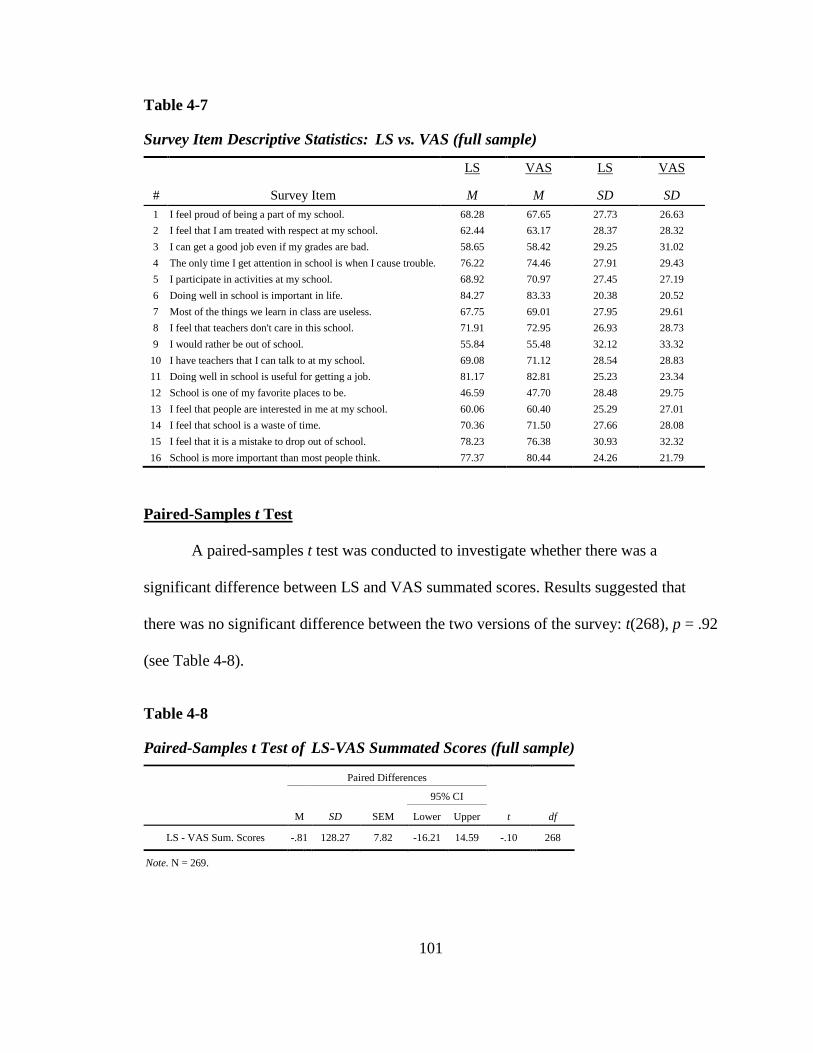
101
Table 4-7
Survey Item Descriptive Statistics: LS vs. VAS (full sample)
# Survey Item
LS
M
VAS
M
LS
SD
VAS
SD
1 I feel proud of being a part of my school. 68.28 67.65 27.73 26.63
2 I feel that I am treated with respect at my school. 62.44 63.17 28.37 28.32
3 I can get a good job even if my grades are bad. 58.65 58.42 29.25 31.02
4 The only time I get attention in school is when I cause trouble. 76.22 74.46 27.91 29.43
5 I participate in activities at my school. 68.92 70.97 27.45 27.19
6 Doing well in school is important in life. 84.27 83.33 20.38 20.52
7 Most of the things we learn in class are useless. 67.75 69.01 27.95 29.61
8 I feel that teachers don't care in this school. 71.91 72.95 26.93 28.73
9 I would rather be out of school. 55.84 55.48 32.12 33.32
10 I have teachers that I can talk to at my school. 69.08 71.12 28.54 28.83
11 Doing well in school is useful for getting a job. 81.17 82.81 25.23 23.34
12 School is one of my favorite places to be. 46.59 47.70 28.48 29.75
13 I feel that people are interested in me at my school. 60.06 60.40 25.29 27.01
14 I feel that school is a waste of time. 70.36 71.50 27.66 28.08
15 I feel that it is a mistake to drop out of school. 78.23 76.38 30.93 32.32
16 School is more important than most people think. 77.37 80.44 24.26 21.79
Paired-Samples t Test
A paired-samples t test was conducted to investigate whether there was a
significant difference between LS and VAS summated scores. Results suggested that
there was no significant difference between the two versions of the survey: t(268), p = .92
(see Table 4-8).
Table 4-8
Paired-Samples t Test of LS-VAS Summated Scores (full sample)
Paired Differences
t df
M SD SEM
95% CI
Lower Upper
LS - VAS Sum. Scores -.81 128.27 7.82 -16.21 14.59 -.10 268
Note. N = 269.
102
Conclusion
Based on the tests conducted above, when summated scores of the full sample
were compared, a paired-samples t test revealed no significant difference between the LS
and VAS item response formats (t = -.10, df = 268, p = .92). Results suggest that the
summated scores of the Identification with School survey are not affected by item
response format.
Summated Scores: School-Level Comparisons
Research question #4
Are there significant mean differences of the summated scores on the LS and VAS versions of the survey between Elementary, Middle, and High School students?
School-Level Summated Score Results
Paired-samples t tests were conducted to investigate whether there was a
significant difference between LS and VAS summated scores for each of the three
school-levels: Upper Elementary, Middle, and High School. Because multiple t tests were
conducted with a single sample, to control for Type I error, Dunnett’s correction41
(Keppel & Wickens, 2004) was used to adjust the alpha level to .016. Results suggest
that there was no significant difference (p > .60) between the two versions of the survey,
regardless of school-level (see Table 4-9).
41 The Dunnett’s correction procedure involved dividing alpha by the number of t tests performed.
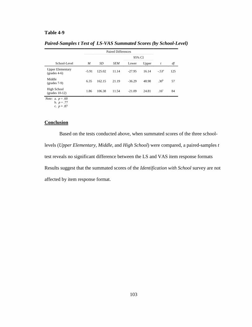
103
Table 4-9
Paired-Samples t Test of LS-VAS Summated Scores (by School-Level) Paired Differences
t df
M SD SEM
95% CI
School-Level Lower Upper
Upper Elementary (grades 4-6)
-5.91 125.02 11.14 -27.95 16.14 -.53a 125
Middle (grades 7-9)
6.35 162.15 21.19 -36.29 48.98 .30b 57
High School (grades 10-12)
1.86 106.38 11.54 -21.09 24.81 .16c 84
Note: a. p = .60 b. p = .77 c. p = .87
Conclusion
Based on the tests conducted above, when summated scores of the three school-
levels (Upper Elementary, Middle, and High School) were compared, a paired-samples t
test reveals no significant difference between the LS and VAS item response formats
Results suggest that the summated scores of the Identification with School survey are not
affected by item response format.
104
Factorial ANOVA
Research question #5
Is there a significant interaction between level of schooling and item response type? If so, was it dependent on item response type?
Main Effects
Levene’s test of equality of variances was conducted and indicated homogeneity
of variance within the school-level groups, F(5, 168) = 1.94, p=.09. A univariate
ANOVA was conducted to determine the effects of item response type on the
Identification with School summated survey scores (see Table 4-11). Main effects were
examined first to determine if differences among the means for the LS and VAS versions
of the survey were significant when averaged over the three levels of schooling. Main
effect results revealed scores were significantly different between school levels, F(2, 168)
= 13.14, p=<.001, partial 2 .135η = . The main effect of item response type yielded an F
ratio of F(1, 168) < 1.00, p=.73, partial 2 .001η = , indicating that item response type did
not have a significant impact on the overall summated scores of the survey.
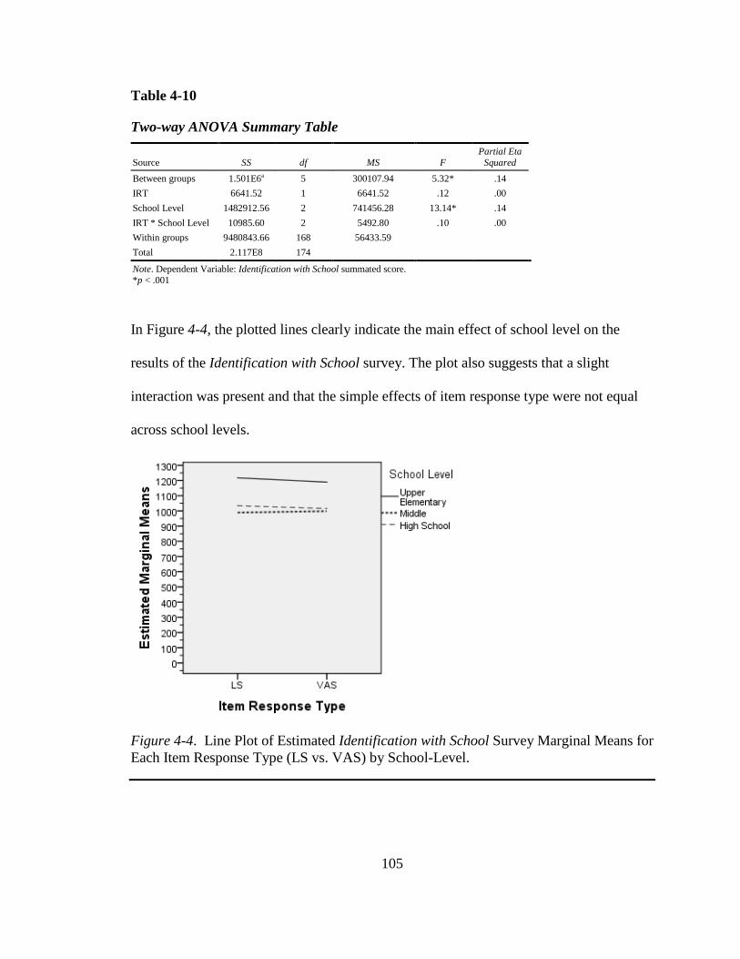
105
Table 4-10
Two-way ANOVA Summary Table
Source SS df MS F Partial Eta
Squared
Between groups 1.501E6a 5 300107.94 5.32* .14
IRT 6641.52 1 6641.52 .12 .00
School Level 1482912.56 2 741456.28 13.14* .14
IRT * School Level 10985.60 2 5492.80 .10 .00
Within groups 9480843.66 168 56433.59
Total 2.117E8 174
Note. Dependent Variable: Identification with School summated score. *p < .001
In Figure 4-4, the plotted lines clearly indicate the main effect of school level on the
results of the Identification with School survey. The plot also suggests that a slight
interaction was present and that the simple effects of item response type were not equal
across school levels.
Figure 4-4. Line Plot of Estimated Identification with School Survey Marginal Means for Each Item Response Type (LS vs. VAS) by School-Level.
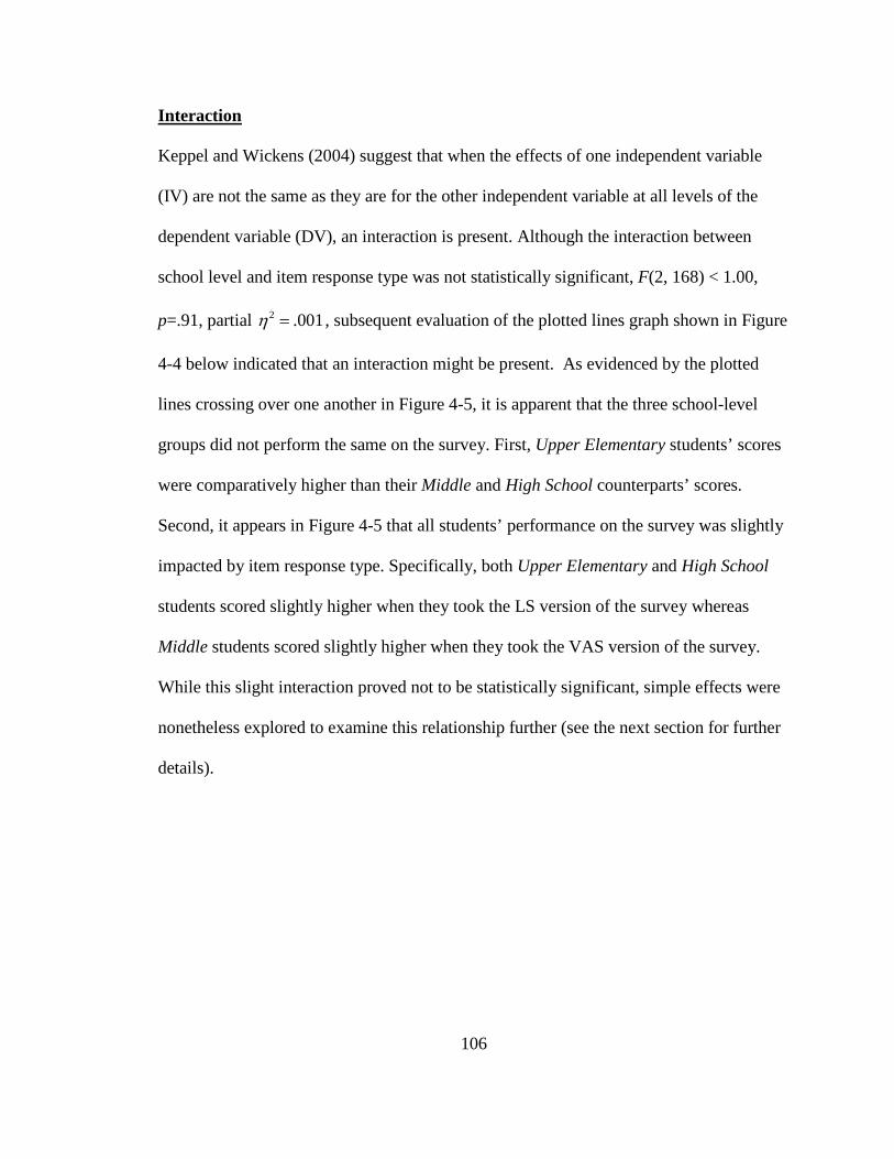
106
Interaction
Keppel and Wickens (2004) suggest that when the effects of one independent variable
(IV) are not the same as they are for the other independent variable at all levels of the
dependent variable (DV), an interaction is present. Although the interaction between
school level and item response type was not statistically significant, F(2, 168) < 1.00,
p=.91, partial 2 .001η = , subsequent evaluation of the plotted lines graph shown in Figure
4-4 below indicated that an interaction might be present. As evidenced by the plotted
lines crossing over one another in Figure 4-5, it is apparent that the three school-level
groups did not perform the same on the survey. First, Upper Elementary students’ scores
were comparatively higher than their Middle and High School counterparts’ scores.
Second, it appears in Figure 4-5 that all students’ performance on the survey was slightly
impacted by item response type. Specifically, both Upper Elementary and High School
students scored slightly higher when they took the LS version of the survey whereas
Middle students scored slightly higher when they took the VAS version of the survey.
While this slight interaction proved not to be statistically significant, simple effects were
nonetheless explored to examine this relationship further (see the next section for further
details).
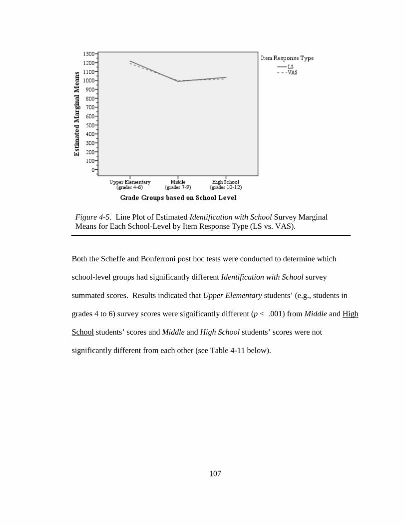
107
Figure 4-5. Line Plot of Estimated Identification with School Survey Marginal Means for Each School-Level by Item Response Type (LS vs. VAS).
Both the Scheffe and Bonferroni post hoc tests were conducted to determine which
school-level groups had significantly different Identification with School survey
summated scores. Results indicated that Upper Elementary students’ (e.g., students in
grades 4 to 6) survey scores were significantly different (p < .001) from Middle and High
School students’ scores and Middle and High School students’ scores were not
significantly different from each other (see Table 4-11 below).
108
Table 4-11
Post Hoc Tests for Multiple Comparisons of School Level
(I) School Level (J) School Level
Mean Difference
(I-J) SE p
95% CI
Lower Upper
Scheffe Upper Elementary (grades 4-6)
Middle 209.60 44.11 p<.01 100.66 318.55
High School 178.29 44.11 p<.01 69.34 287.24
Middle (grades 7-9)
Upper Elementary -209.60 44.11 p<.01 -318.55 -100.66
High School -31.31 44.11 .78 -140.26 77.64
High School (grades 10-12)
Upper Elementary -178.29 44.11 p<.01 -287.24 -69.34
Middle 31.31 44.11 .78 -77.64 140.26
Bonferroni Upper Elementary (grades 4-6)
Middle 209.60 44.11 p<.01 102.93 316.28
High School 178.29 44.11 p<.01 71.62 284.97
Middle (grades 7-9)
Upper Elementary -209.60 44.11 p<.01 -316.28 -102.93
High School -31.31 44.11 1.00 -137.98 75.36
High School (grades 10-12)
Upper Elementary -178.29 44.11 p<.01 -284.97 -71.62
Middle 31.31 44.11 1.00 -75.36 137.98
Note. Dependent Variable: Identification w/School Summated Score. The error term, Mean Square (Error) = 56433.59.
Simple Effects
A simple effect is one that expresses the difference among the means for one
independent variable at a fixed level of the other independent variable (Klockars & Sax,
1986). Simple effects analyze the interaction between variables based on the pattern of
significant and nonsignificant differences in the means. To test for simple effects, the
differences between the LS and VAS were examined for each of the three school levels.
Three separate tests of significance were conducted to determine if the differences
between LS and VAS, for a specific school level, differed significantly. Although a
significant interaction was not present, simple effects were nonetheless examined due to
the pattern observed in Figure 4-5 above, which suggested that a slight interaction was
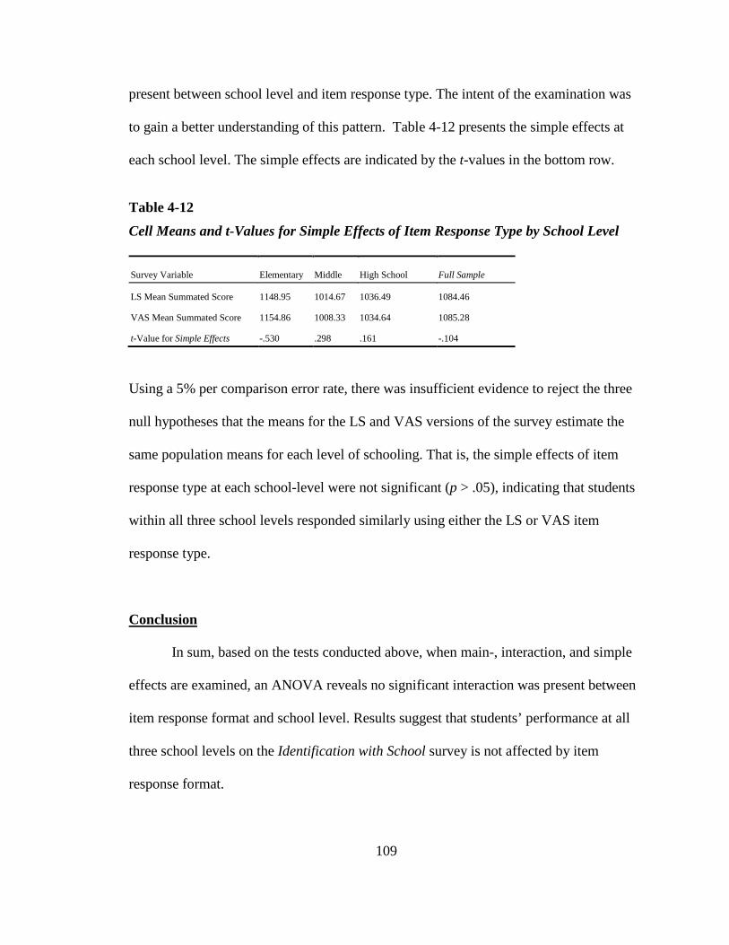
109
present between school level and item response type. The intent of the examination was
to gain a better understanding of this pattern. Table 4-12 presents the simple effects at
each school level. The simple effects are indicated by the t-values in the bottom row.
Table 4-12
Cell Means and t-Values for Simple Effects of Item Response Type by School Level
Survey Variable Elementary Middle High School Full Sample
LS Mean Summated Score 1148.95 1014.67 1036.49 1084.46
VAS Mean Summated Score 1154.86 1008.33 1034.64 1085.28
t-Value for Simple Effects -.530 .298 .161 -.104
Using a 5% per comparison error rate, there was insufficient evidence to reject the three
null hypotheses that the means for the LS and VAS versions of the survey estimate the
same population means for each level of schooling. That is, the simple effects of item
response type at each school-level were not significant (p > .05), indicating that students
within all three school levels responded similarly using either the LS or VAS item
response type.
Conclusion
In sum, based on the tests conducted above, when main-, interaction, and simple
effects are examined, an ANOVA reveals no significant interaction was present between
item response format and school level. Results suggest that students’ performance at all
three school levels on the Identification with School survey is not affected by item
response format.
110
Post-Survey Questionnaire
This section provides a broad understanding of how students typically felt about
using the LS and VAS to respond to questions on the Identification with School survey.
Dichotomous Item Results
Students in both treatment conditions were asked five post-survey questions.
Three of these questions were asked on the Student Opinion Questionnaire (see Appendix
C) and were specific to only the “LS First” condition or the “VAS First” condition. That
is, these three questions were administered immediately following the first survey that
students completed. Thus, roughly only half the sample responded to questions about the
LS and the other half responded to questions about the VAS (depending on which
condition they were assigned to first).42 The remaining two post-survey questions were
asked of all students on the Student Demographic Questionnaire (see Appendix D),
which was administered at the end of the experiment.
In general, roughly 90% of the students indicated that they did not find the items
on the Identification with School survey hard to answer. Overall, students preferred
answering questions with the VAS compared to the LS nearly 3 to 1 (71.4% vs. 27.1%).
For the students who received the LS first, when asked whether the LS enabled them to
pick an answer that closely matched how they felt, students were nearly evenly divided:
roughly half (51%) indicated that the LS did and the other half indicated that it did not.
42 It bears noting that some of the numbers and percentages presented for the Student Opinion Questionnaire are dependent upon the number assigned to a specific initial experimental condition and not of the full sample (N=269).
111
By comparison, for the students who received the VAS first, a clear preference emerged
when they were asked whether the VAS enabled them to choose a response that closely
matched how they felt: More than three-fourths of students who responded indicated that
the VAS let them pick an answer that matched exactly the way they felt.
Lastly, when asked if there were any desired changes to the response options,
60% of students indicated that the LS items did not need different (e.g., less restrictive)
response options and 66% indicated that the VAS did not need a set of provided-response
options (e.g., Likert-type) from which to choose. Table 4-13 presents the quantitative
results of the dichotomous (e.g., Yes/No) items from the Student Opinion Questionnaire
and Table 4-14 presents the quantitative results of the supplementary post-survey
questions that were administered to all students after the experiment (see Appendix D).
Qualitative results of the open-response components of these questions are presented in
the following section.
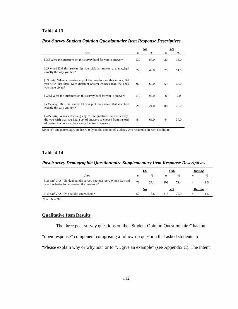
112
Table 4-13
Post-Survey Student Opinion Questionnaire Item Response Descriptives No Yes
Item n % n %
[LS] Were the questions on this survey hard for you to answer? 130 87.0 20 13.0
[LS only] Did this survey let you pick an answer that matched exactly the way you felt?
72 49.0 75 51.0
[LS only] When answering any of the questions on this survey, did you wish that there were different answer choices than the ones you were given?
90 60.0 59 40.0
[VAS] Were the questions on this survey hard for you to answer? 110 93.0 8 7.0
[VAS only] Did this survey let you pick an answer that matched exactly the way you felt?
28 24.0 88 76.0
[VAS only] When answering any of the questions on this survey, did you wish that you had a set of answers to choose from instead of having to choose a place along the line to answer?
84 66.0 44 34.0
Note: n’s and percentages are based only on the number of students who responded in each condition.
Table 4-14
Post-Survey Demographic Questionnaire Supplementary Item Response Descriptives LS VAS Missing
Item n % n % n %
[LS and VAS] Think about the survey you just took. Which way did you like better for answering the questions?
73 27.1 192 71.4 4 1.5
No Yes Missing
[LS and VAS] Do you like your school? 50 18.6 215 79.9 4 1.5
Note. N = 269.
Qualitative Item Results
The three post-survey questions on the “Student Opinion Questionnaire” had an
“open response” component comprising a follow-up question that asked students to
“Please explain why or why not” or to “…give an example” (see Appendix C). The intent

113
of this section is to provide a broad understanding of how students typically felt about
using the LS and VAS to respond to questions on the Identification with School survey.
A review of the post-survey open-response items revealed three specific themes
that captured student sentiment for each of the open-response items. The themes were: 1)
Specificity/Accuracy; 2) Freedom of Response; and 3) Ease of Use. The
Specificity/Accuracy theme comprises student responses that reflect the ability of the LS
or VAS to accurately capture students’ feelings or to specify the strength of their
responses. The Range of Response theme comprises student responses that reflect the
ability of the LS or VAS to allow students the freedom to respond in the manner in which
they wished to respond. Lastly, the Ease of Use theme comprises student responses that
reflect the level of comfort students had while using the LS or VAS to respond and/or the
level of understanding students had of how to use the LS or VAS to convey their
responses.
Likert scale responses.
In general, students who responded negatively to questions about the LS did not
like being forced to choose from a limited set of response options and did not like being
unable to modify the response options to match more precisely their actual response.
Students also expressed that they wanted a neutral mid-point for times when they neither
agreed nor disagreed with the item prompt. Students who responded positively to
questions about the LS thought that it was easier to respond when specific answer choices
were given. In addition, these students expressed that the range of the four LS response
options (Strongly Disagree to Strongly Agree) were sufficient to capture their responses.

114
In particular, some students stated that the LS captured exactly what they were feeling.
Lastly, some students appreciated the four response options because they were easy to
choose from and easy to understand. Table 4-15 below presents several examples of
positive and negative student responses and the general themes associated with these
responses for the LS.
Table 4-15
LS Post-Survey Questionnaire Open-Response Themes and Student Responses
Theme Negative Example Positive Example
Specificity/Accuracy
Because there were no variety in the answers and I was between answers.
On most the questions I found a suitable answer
I have more strong "feelings" than can go into 4 distinct categories. This seems like a male-oriented survey.
[The LS response options] are all the feelings you can have. A neutral button for if you don't know would be helpful.
I wasn't able to give my exact opinion. [The LS response options were] exactly
what I felt
No because the way I felt did not really have an answer that matched my feelings.
Yes it did, because it had the answers that I would pick.
Range of Response I had to be absolute...very frustrating since everything is not in black or white (slight black or slight white).
It had strongly disagree, disagree, strongly agree, and agree. That is perfectly enough.
I wasn't opinionated on many of the questions but was forced to agree or disagree and met some difficulty in doing so.
Yes this survey did let me answer the way I wanted to, because they were easy to answer with the answers provided.
Because some of them I felt different about it instead of agree, strongly agree, disagree, strongly disagree. I wish the answers were broader in some cases.
I think this does not have totally detailed options but it's almost completely satisfying.
Ease of Use
…for some questions it was difficult to determine if I really did disagree or agree. There should of been a 'Maybe' button.
because the choices in this survey are choices that I can understand
I sometimes wanted to make my answer be somewhere between two answers like one time I picked agree but I wanted to pick like something between agree and strongly agree.
I could express myself easily on these questions.
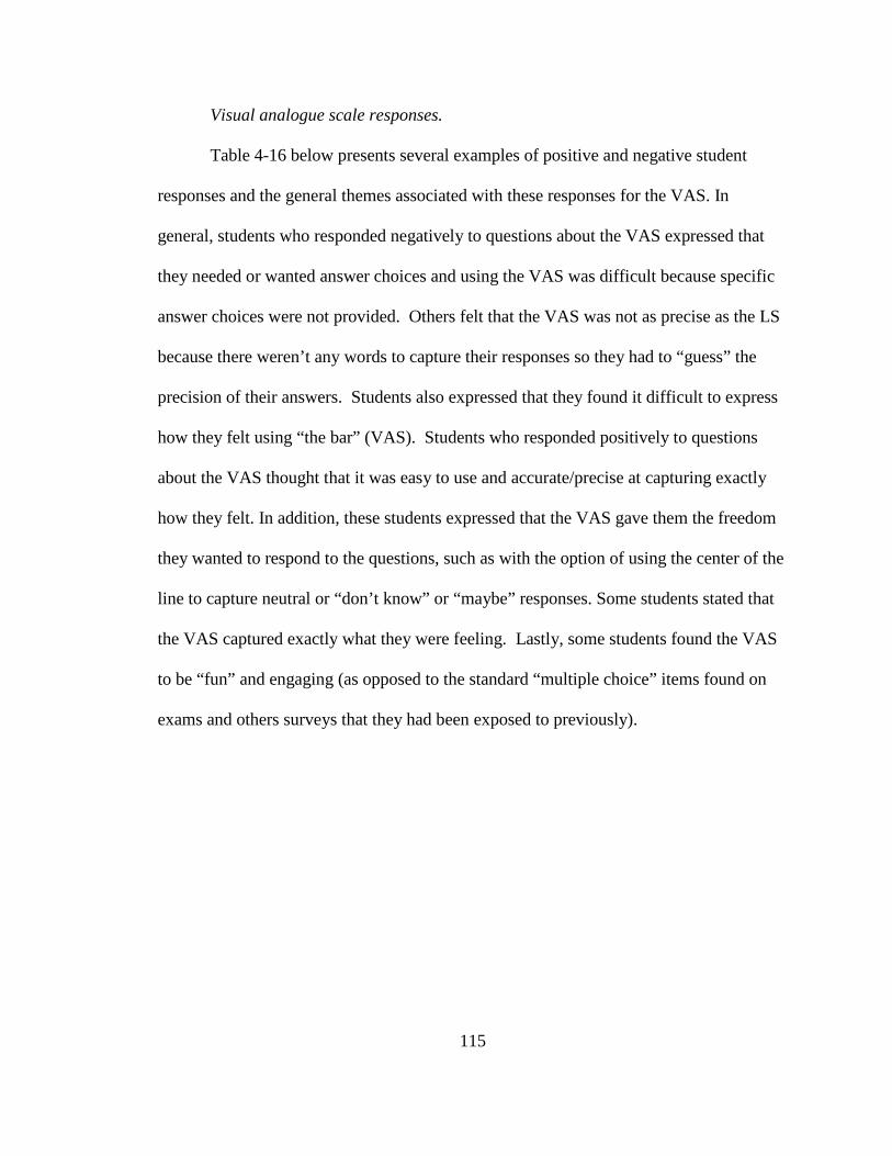
115
Visual analogue scale responses.
Table 4-16 below presents several examples of positive and negative student
responses and the general themes associated with these responses for the VAS. In
general, students who responded negatively to questions about the VAS expressed that
they needed or wanted answer choices and using the VAS was difficult because specific
answer choices were not provided. Others felt that the VAS was not as precise as the LS
because there weren’t any words to capture their responses so they had to “guess” the
precision of their answers. Students also expressed that they found it difficult to express
how they felt using “the bar” (VAS). Students who responded positively to questions
about the VAS thought that it was easy to use and accurate/precise at capturing exactly
how they felt. In addition, these students expressed that the VAS gave them the freedom
they wanted to respond to the questions, such as with the option of using the center of the
line to capture neutral or “don’t know” or “maybe” responses. Some students stated that
the VAS captured exactly what they were feeling. Lastly, some students found the VAS
to be “fun” and engaging (as opposed to the standard “multiple choice” items found on
exams and others surveys that they had been exposed to previously).
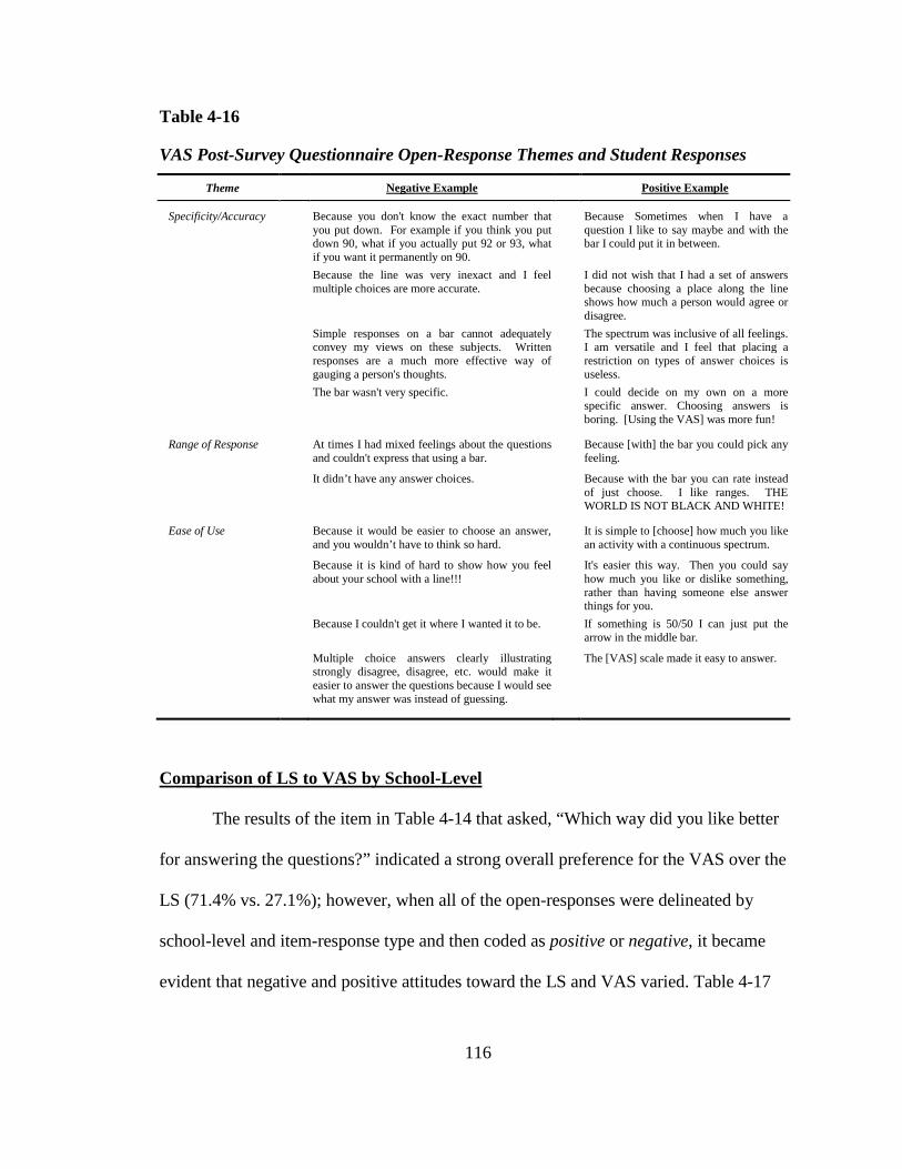
116
Table 4-16
VAS Post-Survey Questionnaire Open-Response Themes and Student Responses
Theme Negative Example Positive Example
Specificity/Accuracy Because you don't know the exact number that you put down. For example if you think you put down 90, what if you actually put 92 or 93, what if you want it permanently on 90.
Because Sometimes when I have a question I like to say maybe and with the bar I could put it in between.
Because the line was very inexact and I feel multiple choices are more accurate.
I did not wish that I had a set of answers because choosing a place along the line shows how much a person would agree or disagree.
Simple responses on a bar cannot adequately convey my views on these subjects. Written responses are a much more effective way of gauging a person's thoughts.
The spectrum was inclusive of all feelings. I am versatile and I feel that placing a restriction on types of answer choices is useless.
The bar wasn't very specific. I could decide on my own on a more specific answer. Choosing answers is boring. [Using the VAS] was more fun!
Range of Response At times I had mixed feelings about the questions and couldn't express that using a bar.
Because [with] the bar you could pick any feeling.
It didn’t have any answer choices. Because with the bar you can rate instead of just choose. I like ranges. THE WORLD IS NOT BLACK AND WHITE!
Ease of Use Because it would be easier to choose an answer, and you wouldn’t have to think so hard.
It is simple to [choose] how much you like an activity with a continuous spectrum.
Because it is kind of hard to show how you feel about your school with a line!!!
It's easier this way. Then you could say how much you like or dislike something, rather than having someone else answer things for you.
Because I couldn't get it where I wanted it to be. If something is 50/50 I can just put the arrow in the middle bar.
Multiple choice answers clearly illustrating strongly disagree, disagree, etc. would make it easier to answer the questions because I would see what my answer was instead of guessing.
The [VAS] scale made it easy to answer.
Comparison of LS to VAS by School-Level
The results of the item in Table 4-14 that asked, “Which way did you like better
for answering the questions?” indicated a strong overall preference for the VAS over the
LS (71.4% vs. 27.1%); however, when all of the open-responses were delineated by
school-level and item-response type and then coded as positive or negative, it became
evident that negative and positive attitudes toward the LS and VAS varied. Table 4-17
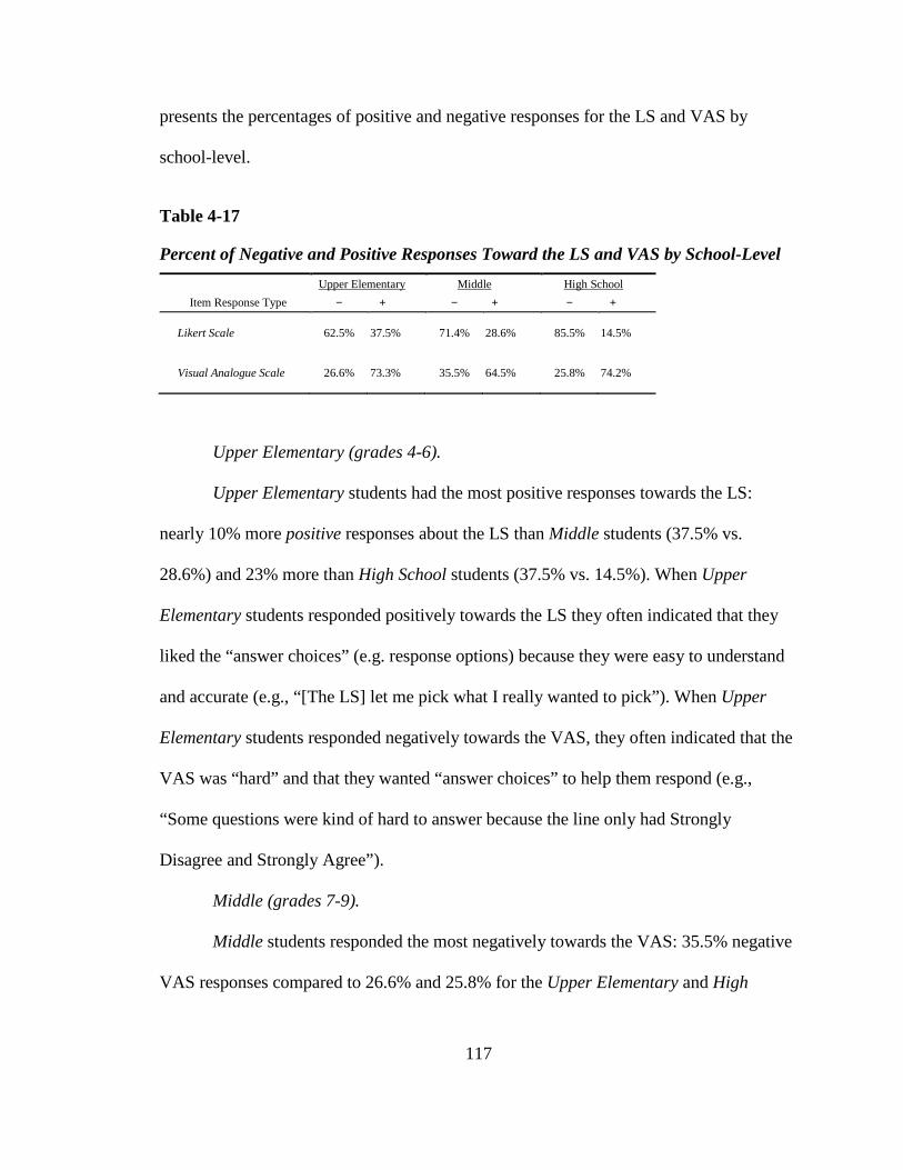
117
presents the percentages of positive and negative responses for the LS and VAS by
school-level.
Table 4-17
Percent of Negative and Positive Responses Toward the LS and VAS by School-Level Upper Elementary Middle High School
Item Response Type − + − + − +
Likert Scale 62.5% 37.5% 71.4% 28.6% 85.5% 14.5%
Visual Analogue Scale 26.6% 73.3% 35.5% 64.5% 25.8% 74.2%
Upper Elementary (grades 4-6).
Upper Elementary students had the most positive responses towards the LS:
nearly 10% more positive responses about the LS than Middle students (37.5% vs.
28.6%) and 23% more than High School students (37.5% vs. 14.5%). When Upper
Elementary students responded positively towards the LS they often indicated that they
liked the “answer choices” (e.g. response options) because they were easy to understand
and accurate (e.g., “[The LS] let me pick what I really wanted to pick”). When Upper
Elementary students responded negatively towards the VAS, they often indicated that the
VAS was “hard” and that they wanted “answer choices” to help them respond (e.g.,
“Some questions were kind of hard to answer because the line only had Strongly
Disagree and Strongly Agree”).
Middle (grades 7-9).
Middle students responded the most negatively towards the VAS: 35.5% negative
VAS responses compared to 26.6% and 25.8% for the Upper Elementary and High

118
School students, respectively. When Middle students responded negatively towards the
VAS, the responses were often related to the VAS making it “harder” to express
themselves (e.g., “At times I had mixed feelings about the questions and couldn't express
that using a bar”) and being “less specific” than the LS (e.g., [“Having LS response
options] would make my answers more specific than just being kinda random [as with the
VAS]”). Of the nearly 30% of Middle students who responded positively towards the LS,
many indicated that they prefer “multiple choice” (e.g. LS) questions because choosing
from a pre-determined or supplied set of responses was “easier” than having to determine
on one’s own a response from within the wide range of possibilities that the VAS
presents (e.g., “I think a [set of LS response options] would have been better than a line
because there are more choices than a random spot on the line….Advice for the future:
MAKE THESE QUESTIONS MULTIPLE CHOICE INSTEAD OF A STINKIN
LINE!”).
High School (grades 10-12).
Of the three school-levels, High School students responded the most negatively
towards the LS: 85.5% negative LS responses compared to 63.5% and 71.4% for Upper
Elementary and Middle, respectively. They responded most positively towards the VAS:
74.2% positive VAS responses compared to 73.3% and 64.5% for Upper Elementary and
Middle, respectively. When High School students responded negatively towards the LS,
they most often complained that LS response options failed to adequately capture the
intensity of their responses (e.g., “I felt at times that I could have marked between
choices. I did not agree with the choices [the LS provided]”). High School students, in

119
particular, resented the “limited” choices of the LS and did not like being “forced” to
choose from only one of four responses (e.g., “[The LS response options] didn't let me
pick an answer that matched exactly the way I felt because on some questions I felt like
only sometimes I agreed rather than completely disagree or agree”). Lastly, it is
interesting to note that in comparison to the other two groups of students, High School
students wanted more control over how their responses were interpreted. In responses
related to both the LS as well as the VAS, several High School students indicated a desire
to have an opportunity to “explain” their responses (e.g., “Each time [I responded with
LS response options] I think I would have liked a better chance to explain my reasoning”;
and “Simple responses on a bar [VAS] cannot adequately convey my views on these
subjects. Written responses are a much more effective way of gauging a person's
thoughts”). Such a desire to more fully explain responses was not mentioned by students
in the other two school levels.
Summary
The analyses presented in this chapter provide evidence that the Identification
with School survey is a reliable measure of students’ identification with school for grades
4-12 regardless of the item response type used. Results also suggest that the LS and VAS
versions of the survey yielded nearly identical results, thus indicating that item response
type did not affect the results of the Identification with School survey in this study. In
addition, results of the post-survey student questionnaires suggest that students preferred
120
the VAS over the LS 3 to 1 when asked which item response type they liked best. While
students were nearly evenly split when asked if they thought the LS allowed them to pick
an answer that matched exactly how they felt (49%: “No” vs. 51%: “Yes”), a clear
majority of students (76%: “Yes” vs. 24%: “No”) indicated that the VAS allowed them to
respond in a manner that captured their feeling exactly. Lastly, while all three school
levels had a greater percentage of positive responses than negative towards the VAS than
the LS, High School students had the highest percentage of positive responses.
Conversely, of the students who responded positively towards the LS, Upper Elementary
students had the greatest percentage of positive responses. These results are consistent
with Piagetian stages of child development in that the younger, Upper Elementary and
Middle students were more inclined to prefer the “concrete” response options of the LS
whereas the older, High School students were more inclined to prefer the VAS because
they are more independent thinkers and would be more likely to have an aversion to any
limitations of their unique self-expression. A more detailed discussion of this study’s
findings is presented in the following chapter.

121
Chapter 5: Discussion and Conclusion
In this chapter, results from the previous chapter are briefly summarized and
discussed. Limitations and the implications of the results of this study are also presented,
and suggestions for future research are made.
Overview of Findings
The purpose of this study was to investigate whether changing the response
format from LS to VAS on the Identification with School survey affects the underlying
factor structure, reliability, and summated scores of the survey across three levels of
schooling: Upper Elementary, Middle, and High School. Additionally, this study sought
to examine the main, interaction, and simple effects of item response type and school
level (the two predictor variables) on scores yielded by the survey (the outcome variable).
The primary findings of this study reveal that: 1) the VAS yields a factor structure similar
to the LS; 2) the VAS is equally reliable as the LS in terms of internal consistency and
test-retest reliability; 3) the VAS yields nearly identical summated scores as the LS
regardless of school level; and 4) the VAS was preferred by a majority of students across
all three school levels. Additionally, the results of an ANOVA conducted to examine
school level and response mode effects indicate that while school level had a statistically
significant main effect on summated survey scores and response mode did not, the mode
effect was invariant across school levels. In other words, while there were significant
differences in mean summated scores across school levels, these differences were

122
consistent across the LS and VAS response formats. In total, these findings suggest that
while student performance on the Identification with School survey was not affected by
item response format, student preference for the VAS format was nonetheless made
evident by their answers to items on the post-survey questionnaire.
Discussion
Consistency of Findings
The findings from this study are consistent with the work of other investigators
who have either administered the Identification with School survey (Ruiz, 2002; Voelkl,
1996) or compared the effects of using the Likert scale (LS) versus the visual analogue
scale (VAS) item response formats with children (Berntson & Svensson, 2001; van
Laerhoven et al., 2004). First, the results of Principal Components Analysis (PCA),
which revealed that the factor structure of the LS and VAS versions of the Identification
with School survey was unidimensional, support the findings originally reported by
Voelkl (1996), who conducted the first study that explores this topic. Second, the results
of the internal consistency reliability tests of the Identification with School survey, which
yielded identical LS and VAS Cronbach’s alpha reliability coefficients of a = .83,
indicate that this survey’s items are highly consistent and provide evidence that the
yielded scores are reliable. The findings on reliability are consistent with findings by
Ruiz (2002) and Voelkl (1996), who reported Cronbach’s alpha reliability coefficients of
.80 and .84, respectively for the Identification with School survey. Third, while no
123
previous study has examined the test-retest reliability of the Identification with School
survey, similar research on the test-retest reliability of the VAS has demonstrated that it
does not influence this coefficient of stability (Funke & Reips, 2007a). As such, the
findings of this study, which suggest that the scores produced by the survey were
statistically similar across both forms of the survey and within the levels of schooling, are
consistent with previous research. Moreover, given that item response type did not have
a statistically significant effect on students’ summated scores, it appears that these two
scales are, in effect, interchangeable.
Explaining the Differences in Scores Between School Levels
While there were statistically significant differences between the Upper
Elementary students' summated scores on the Identification with School survey and the
scores of the other two school levels, the findings of this study suggest that the observed
difference was not a function of item response type. The simplest explanation for why
the Upper Elementary students’ summated scores were higher is that they genuinely do
enjoy school more than their Middle and High School counterparts and therefore they
more strongly and positively identify with school and school-related outcomes. A
slightly more complex explanation for the higher summated scores achieved by the
Upper Elementary students compared to the Middle and High School students could
possibly be attributed to the survey topic and the questions that were asked on the
Identification with School survey. In particular, the research literature suggests that
younger children may be more prone to “acquiescing” than older children, meaning
124
younger children are more likely to respond in ways they view as more socially desirable
or in ways they feel would “please” adults (Ormrod, 1995). This phenomenon could
explain the Upper Elementary students’ more positive identification with school and
corresponding higher summated survey scores on the Identification with School survey
compared to their Middle and High School student counterparts.
Lastly, a possible explanation for why the students in the Middle school level
scored lowest on the survey of all three groups is provided by Eccles, Midgley, Wigfield,
Buchanan, Reuman, Flanagan, et. al, (1993), who suggest that in addition to the negative
psychological changes often associated with this age range as they develop, young
adolescents may experience a “mismatch” between their personal needs and the
opportunities provided in their school environment that can impact their motivation and
self-perceptions. As such, the younger adolescent students who participated in this study
may have experienced a greater disconnect between themselves and the schools they
attended, which could have, in turn, affected their summated scores on the Identification
with School survey.
Explaining the Differences in Item Response-Type Preference
It is interesting to note that while students’ responses were consistent across forms
and their scores within school-level were not statistically significantly different, all of the
students expressed a preference for one or the other item response type. While most
students, irrespective of school level, expressed a preference for the VAS over the LS,

125
this preference was not universal. Two possible explanations for students’ item response-
type preference are discussed below.
Piaget’s stages of development.
The present study’s findings highlight possible age effects in the use of surveys
and are consistent with Piagetian stages of child development; specifically, younger
students are more likely to prefer the concreteness of the LS responses and older students
are more likely to prefer the freedom of expression that the VAS provides. As discussed
in Chapter 2,43 although children in the concrete operational stage may be capable of
many forms of logical thought, their cognitive development is in its early stages and thus
they may have difficulty grasping hypothetical scenarios that cannot be directly observed
or experienced. They may also struggle with proportional reasoning, which is evident in
the responses of some students in this study who indicated that it was hard for them to
convey their feelings on a line (VAS). These cognitive limitations may have had an
impact on some students’ ability to grasp the concept of the VAS response format
(although no studies to date have investigated the legitimacy of this claim). Further, their
cognitive limitations could explain why more than one-third of Upper Elementary
students preferred the LS with its “concrete” set of verbal anchors and why they thought
the LS was “easier to complete” than the VAS. By comparison, children in the formal
operations stage begin to be able to think about concepts that are abstract, hypothetical, or
contrary-to-fact and become more independent thinkers capable of unique self-
expression. A number of abilities essential for sophisticated reasoning also emerge
43 In the Children and Surveys section under the Cognitive Development sub-heading.

126
during this developmental stage that enable these children to use and understand
continuums in their reasoning. This was evident among many of the High School
students in this study who not only understood how to use the VAS, but also expressed a
strong preference for it over the LS as the VAS allowed them to convey precisely how
they felt.
While Piaget's focus on qualitative child development had an important impact on
education, it is important to note that he did not specifically apply his theory to education.
Nonetheless, many educational programs are built upon the belief that children should be
taught at the level for which they are developmentally prepared. That being said, it is
generally accepted today that all children will not, as Piaget maintained, automatically
move to the next stage of development as they mature. An additional criticism of Piaget’s
work is that it failed to take into consideration social or cultural factors that likely
influence the rate in which children proceed (or not) from one developmental stage to the
next. As such, it is important to note that a child’s home environment could have an
affect on her emotional and cognitive development. To that end, the lack of uniformity in
student preferences observed across school levels for either the LS or VAS could be a
function of students at, above, or below their Piagetian-defined level of development.
The “digital generation”: Today’s media-savvy students.
While Piagetian developmental stages can be helpful with explaining student
preference for either the LS or VAS when student preference is consistent with their age,
his stages offer little insight into why some of the younger students preferred the VAS
and some older students preferred the LS. A simple explanation for why a majority of all
127
students preferred the VAS is that today’s students are part of a new “digital generation”
of computer-savvy children, some of whom spend up to 6.5 hours a day with digital
media (Rideout, Roberts, & Foehr, 2005). 44 As a result, many students today are
naturally adept with technology and used to manipulating things on a computer, whether
it be an avatar in a game, text on a page, or an image in a drawing program/photograph.
To that end, the VAS may be more similar to the way they use a computer and may also
make them feel more involved in the process of answering questions. A possible
explanation for the younger students’ preference for the VAS could be that their
preference is a function of their advanced cognitive development (in comparison to their
peers). For example, it is possible that these students were gifted or high academic
achievers and therefore have more in common with older students than their younger
peers. Similarly, for the older students who preferred the LS, they may be less
academically advanced, or developmentally behind their peers emotionally or
cognitively. Additionally, it could be possible that these students were not motivated to
complete the survey.
Student Motivation Effects
There are three related problems that investigators face when conducting survey
research. The first problem is respondent fatigue, which can potentially affect student
44 According to Rideout, Roberts, & Foehr (2005), “Young people today live media-saturated lives, spending an average of nearly 6½ (6:21) hours a day with media. Across the seven days of the week, that amount is the equivalent of a full-time job, with a few extra hours thrown in for overtime (44½ hours a week). Indeed, given that about a quarter (26%) of the time young people are using media, they’re using more than one medium at a time (reading and listening to music, for example), they are actually exposed to the equivalent of 8½ hours a day (8:33) of media content, even though they pack that into less than 6½ hours of time.”
128
motivation to complete the survey. The second problem is attrition, which may be the
effect of low student motivation. These two problems then lead to the third problem,
item non-response.
Fatigue.
According to Tourangeau (1984), responding to survey questions requires that
respondents proceed through four consecutive stages of cognitive processing: 1)
understand and interpret the question; 2) search their memory for relevant information
and retrieve it; 3) integrate the information into a judgment or cogent response; and 4)
respond or report the information in a way that clearly and concisely conveys their (the
respondent’s) intended meaning. If a respondent carefully goes through all four of these
steps each time she answers a question on a survey, then she has “optimized” her
response (Krosnick, 1991). If the respondent simply provides a superficial response that
required very little cognitive effort, then she is guilty of “satisficing" (1991), meaning her
response was not as accurate or complete as it could have been had he gone through
Tourangeau’s four optimizing steps. Of course, even for the most highly motivated
respondents who may strive to optimize every single response, there is a limit to the
considerable amount of mental effort that can be reasonably expended (and expected)
while responding to a survey.
Respondents may experience fatigue if they require extensive periods of time to
respond to a series of challenging items or to complete a lengthy survey. Given that there
were a number of students in this study who indicated that the VAS was “harder” than the
LS, it is possible that VAS items may require more cognitive resources when responding

129
than LS items. As such, VAS items may call for an increase in cognitive load (e.g,
making students think more about their responses), which may facilitate respondent
fatigue. Additionally, by requiring students to supply responses by contemplating the
magnitude of each response in terms of a continuous scale and then sliding the locator
along a continuum, more time may be required to respond to VAS items compared to LS
items. For longer surveys, this may accumulate into increased administration time and
increased respondent fatigue, which may lead to higher levels of item nonresponse or
respondent attrition.
Attrition.
When respondents leave the study prior to completing all the questions on the
survey, the possibility of error bias is introduced into the survey’s results because of
potentially systematic differences between those who remained in the study and those
who dropped out. In the present study, there were several respondents who answered
only the first few questions and then dropped out of the study. It is not clear whether
these respondents ran out of time, or became bored or frustrated, or whether the survey
was simply accessed out of curiosity (which could have happened with teachers checking
out the survey before administering it to students). Because respondent identities were
anonymous, it is not possible to determine the cause of attrition.
Item nonresponse.
Practically all surveys are accompanied by a loss of information because of item
nonresponse. There are a number of reasons respondents may not answer certain items
including their belief that the question(s) is too sensitive, embarrassing, or irrelevant.

130
Nonresponse can also occur if the respondent does not know the answer or feels that the
question is too difficult. Lastly, nonresponse can occur if the respondent feels that the
question requires too much effort to respond. In the present study, while it is not possible
to determine the reason for specific item nonresponse, post-survey questionnaire
responses provide some evidence that students may have struggled with the question
being asked or may have become frustrated with either the limited options of the LS or
the lack of specific response options for the VAS.
Summary
It is possible that while item response type may not have a statistically significant
affect on student responses, it may have a practically significant affect on student
motivation to respond and to more actively engage in taking a survey. Increasing
motivation for and engagement in the survey process by matching item response types
with the cognitive developmental stage of students (e.g., LS with lower grades and VAS
with upper grades) may be a strategy for survey researchers to attempt to decrease the
effects of issues such as respondent fatigue, attrition, and item nonresponse on study
results.

131
Strengths and Limitations of the Study
Strengths
This study had four primary strengths. First, the experimental design of the study
was particularly strong. One of the benefits of doing an experimental design is the strong
internal validity. As such, the results of this study are more likely to be attributed to the
treatments rather than to subject characteristics threats or other confounding factors, and
one can have a high level of confidence in the conclusions drawn and inferences made
about the results as they pertain to the students in this study. Second, by using random
assignment I was able to provide evidence of design control and reduce the likelihood
that any differences between treatment conditions were systematically related to the
treatments (Shadish, Cook, & Campbell, 2001). Third, by administering both the LS and
VAS versions of the survey to all students, I was able to obtain a coefficient of stability
and demonstrate a high degree of consistency in students’ responses and stability in their
summated scores on the Identification with School survey. Fourth, by utilizing multiple
analytical approaches, I was able to provide psychometric, descriptive, and applied
evidence that the VAS was essentially interchangeable with the LS in this study.
Limitations
There are several limitations to this study that may affect the generalizability of
the findings presented here, and thus the results presented should be interpreted with
caution. First, this study’s sample comprised students in Grades 4-12 who volunteered to
participate; as a result, the sample may not be representative of the population of 4th

132
through 12th grade students in the United States. Therefore, findings of this study may not
necessarily be generalizable to all US students in grades 4-12.
Second, students’ previous computer experience, level of keyboarding skills,
mouse manipulation proficiency, or degree of comfort taking computer-based surveys
was not assessed. These skills could have affected the ease with which students were able
to respond to LS and VAS items or could have affected students’ attitudes toward the LS
and/or VAS. Further, considering that students were not asked about their degree of
computer proficiency or level of comfort with online survey technology, it was not
possible to estimate whether taking the survey on a computer had any effect on student
performance or on their attitudes towards school or item response type. Nevertheless,
there is insufficient evidence to suggest that a lack of previous computer experience was
in any way systematic. Moreover, because random assignment was used both
experimental groups were probabilistically equalized; therefore, even if this characteristic
were present in the sample, it is likely to have been randomly spread across the groups
and thus not necessarily a cause for bias.
A third limitation is that a pre-assessment to determine student reading level was
not administered. Although the readability of the Identification with School survey and
post-survey questionnaires was tested using the Flesch-Kincaid Index (Flesch, 1948) and
results indicated that the reading level of the items was appropriate for 4th grade students,
it was likely that not all participants were able to read at the 4th grade reading level or
higher. Nonetheless, given the primary exclusion criterion that students had to be in 4th
through 12th grade in order to participate, I assumed for the purposes of this study that all

133
participants read at the 4th grade level or higher and fully understood the survey
directions and the items on the survey and post-survey questionnaires. It bears noting that
while it is highly probable that reading ability would have affected only a small portion
of the sample (most likely those students in lower grades who were reading below grade
level) and therefore may have affected some students’ responses, the effect across the
sample is likely to have been minimal. Moreover, given the high test-retest reliability
achieved with this sample and the numerous examples of coherent responses to the post-
survey questionnaires provided by students at all school levels, there is sufficient
evidence to suggest my assumption that students understood the questions on the survey
was warranted.
A fourth and final limitation is that there was some evidence that not all students
made a concerted effort to complete the survey or to take the survey seriously. In
particular, there were incidences of missing responses and unintelligible and profane
responses to open-response items at all school levels. Administering the survey to
students during the last few weeks of the school year and having no consequences or
rewards for performance on the Identification with School survey may have decreased
some students’ motivation for completing the online survey. Although it was not
possible to determine their motivation for skipping questions or responding
inappropriately, it was assumed that these students demonstrated a conspicuous lack of
motivation, which could have influenced their recorded or interpretable responses to the
Identification with School survey. To counteract this possible biasing affect, whenever
possible, blatant examples of student indifference—such as the use of the same response
134
throughout the survey or response to only a few items—were cause for the student’s
exclusion from analyses. This, in part, was the reason the sample was reduced initially
from more than 450 down to 269. Exclusion of less obvious examples of student
indifference—such as missing-, profane-, or unintelligible responses on only a few
items—were decided on a case-by-case basis.
Implications of the Study
The accurate and reliable assessment of students’ perceptions of their well-being
and experiences at school and in the classroom is critical for educational research and
practice. As such, the results of this study have two primary implications for educational
survey research. First, given that item response type appears not to have affected student
responses on the Identification with School survey and that this finding was invariant
across school levels, it is possible that survey designers may be able to use these item
response types interchangeably on other surveys. Second, given that most students
expressed a preference for the VAS over the LS, there may be implications for both
survey designers and educational researchers with regard to designing and/or selecting a
survey that may increase student motivation to remain engaged until completion. It bears
noting, however, that because the extent of student preference for either item response
type differed across school levels in this study (with larger percentages of students in
lower grades preferring the LS than in higher grades) and because younger students often
find the LS to be “easier” than the VAS, it may be advisable for survey designers and

135
researchers to employ LS for lower grade levels and VAS for upper grade levels if
increasing motivation is a factor when deciding item response type.
Suggestions for Future Research
In general, further research is needed to examine factors that might increase or
maximize the likelihood that students provide accurate, reliable, and valid self-reports on
surveys. Although the results of this study suggest the two item response options used
were virtually interchangeable when administered online, research should explore the
circumstances under which the VAS might be more appropriate versus the LS and vice
versa in education. This is important for three reasons outlined in detail below.
First, further research is necessary because virtually no studies have been
conducted in education to directly compare the LS and VAS with K-12 populations, it
remains unclear whether equivalent LS and VAS versions of a survey that measure
objective phenomena (e.g., with discernibly or verifiably “correct” responses) would
yield results similar to those obtain from this study, which measured subjective
phenomena (e.g., feelings or attitudes). If, for example, findings suggest objective
phenomena are best measured with LS and subjective phenomena are best measured with
VAS, then there may be implications for the types of questions asked with LS or VAS
response options on surveys of K-12 populations.
Second, further research is necessary because children’s reasoning for preferring
one item response type over the other (or for completing a survey vs. choosing not to,
136
etc.) can vary so widely. As such, it may be difficult for survey designers and
educational researchers to identify when, for example, or with whom the LS may be the
best option and when the VAS might work better. Thus, in an effort to further explore the
extent to which the LS and VAS affect children’s judgments and motivation, researchers
should consider including a qualitative component to their survey research design to ask
students what they are thinking as they respond to LS versus VAS survey items.
Third and finally, further research is necessary to compare the LS and VAS item
response types using a larger, nationally representative sample comprising the numerous
subgroups in today’s schools such as English-language learners or students receiving
special education services, etc. Research suggests that survey responses are less valid and
reliable when respondents have lower motivation, lower cognitive ability, or have
become fatigued (Krosnick, 1991). Thus, if a student whose first language is not English
or who has a learning disability struggles to read and/or interpret survey items, she is
more likely to become fatigued and/or less motivated to complete the survey and her
results will be less valid and reliable than they would have been had her special needs
been addressed in the survey design. While no studies to date in education have examined
how students receiving special education services respond to the LS or VAS, there is
some evidence in the pain literature that children for whom English is a second language
may prefer the VAS over the LS because they find it more intuitive and easier to
understand (Abu-Saad, Kroonen, & Halfens, 1990).
137
Final Conclusions
The primary goal of this study was to examine whether changing the item
response format of a survey from Likert-scale to visual analogue scale would affect factor
structure, internal consistency and test-retest reliability, or summated scores. The
analyses presented above contribute to the evidence that the Likert scale and visual
analogue scale are virtually interchangeable with the exception of student preference,
which was strongly in favor of the VAS. Since children and adolescents often report
strong preferences for what they eat, what they wear, what they watch on television or
listen to on the radio, etc. and since satisfying (or not satisfying) these preferences can
impact motivation, preference and motivation may be important factors for educational
researchers to consider when deciding on surveys to use with student populations. That
is, if students prefer the VAS over the LS, then it makes sense for educational researchers
to consider using the VAS response option instead of the LS if only to encourage students
to be more engaged in the survey and to potentially reduce survey fatigue. Given the
findings of this study in conjunction with the extent to which students preferred using the
VAS over the LS, use of the VAS in future Web-based survey research with students in
4th through 12th grade is recommended.
138
References
Abu-Saad, H. (1984). Assessing children's responses to pain. Pain, 19, 163-171. Abu-Saad, H., & Holzemer, W. (1981). Measuring children’s self-assessment of pain. Issues in Comprehensive Pediatric Nursing, 5(5), 337-349. Abu-Saad, H., Kroonen, E., & Halfens, R. (1990). On the development of a multidimensional Dutch pain assessment tool for children. Pain, 43, 249-256. Ahearn, E.P. (1997). The use of visual analog scales in mood disorders: A critical review. Journal of Psychological Research, 31(5), 569-579. Aitken, R.C. (1969). Measurement of feelings using visual analogue scales. Proceedings of the Royal Society of Medicine: Section of Measurement in Medicine, 62(10), 989-992. Alwin, D.F. (2007). Margins of error. Hoboken, NJ: John Wiley & Sons, Inc. Aquilino, W. (1994). Interview mode effects in surveys of drug and alcohol use. Public Opinion Quarterly, 58, 210-240. Aquilino, W., & LoSciuto, L. (1990). Effect of interview mode on self-reported drug use. Public Opinion Quarterly, 54, 62-395. Armstrong, G D. (1981). Parametric statistics and ordinal data: A pervasive misconception. Nursing Research, 30(1), 60-62. Averbuch, M., & Katzper, M. (2004). Assessment of visual analog versus categorical scale for measurement of osteoarthritis pain. Journal of Clinical Pharmacology, 44, 368-372. Berntson, L., & Svensson, E. (2001). Pain assessment in children with juvenile chronic arthritis: A matter of scaling and rater. Acta Paediatrica, 90, 1131-1136. Best Evidence Encyclopedia (2008). What is an effect size? Retrieved May 5, 2008 from, http://www.bestevidence.org/resources/general/faq.pdf Blalock, H.M., Wells, C.S., & Carter, L.F. (1970). Statistical estimation with random measurement error. Sociological Methodology, 2, 75-103.
139
Bond, T.G., & Fox, C.M. (2001). Applying the Rasch model: Fundamental measurement in the human sciences. Mahwah, NJ: Lawrence Erlbaum Associates, Inc. Borgers, N., Hox, J., & Sikkel, D. (2003). Response quality in survey research with children and adolescents: The effect of labeled response options and vague quantifiers. International Journal of Public Opinion Research, 15(1), 83-94. Bowling, A. (1998). Research methods in health: Investigating health and health services. Philadelphia: Open University Press. Bowling, A. (2005a). Mode of questionnaire administration can have serious effects on data quality. Journal of Public Health, 27(3), 281–291. Bowling, A. (2005b). Just one question: If one question works, why ask several? Journal of Epidemiology and Community Health, 59, 342-345. Brunier, G., & Graydon, J. (1996). A comparison of two methods of measuring fatigue in patients on chronic haemodialysis: Visual analogue versus Likert scale. International Journal of nursing Studies, 33, 338-348. Buja, A., & Eyuboglu, N. (1989). Remarks on parallel analysis. Multivariate Behavioral Research, 27, 509-540. Cattell, R.B., & Vogelmann, S. (1977). A comprehensive trial of the scree and KG criteria for determining the number of factors. Multivariate Behavioral Research, 12, 289-325. Chambers, C.T., & Johnston, C. (2002). Developmental differences in children’s use of rating scales. Journal of Pediatric Psychology, 27, 27-36. Champion, G.D., Goodenough, B., von Baeyer, C.L., Thomas, W. (1998). Measurement of pain by self-report. In G. Finley & P. McGrath (Eds.), Progress in Pain Research and Management: Vol. 10 (pp. 123-160). Seattle: IASP Press. Cliff, N. (1988). The eigenvalue greater than one rule and the reliability of components. Psychological Bulletin, 103, 276-279. Cohen, J. (1988). Statistical power analysis for the behavioral sciences. Hillsdale, NJ: Lawrence Erlbaum Associates. Cook, C., Heath, F., Thompson, R. & Thompson, B. (2001). Score reliability in Web or Internet-based surveys: Unnumbered graphic rating scales versus Likert-type scales. Educational and Psychological Measurement, 61, 697-706.
140
Couper, M.P. (2000). Web surveys: a review of issues and approaches. Public Opinion Quarterly, 64(4), 464-494. Couper, M.P., Tourangeau, R., & Conrad, F. G. (2006). Evaluating the effectiveness of visual analog scales: A web experiment. Social Science Computer Review, 24(2), 227-245. Cremeens, J., Eiser, C., & Blades, M. (2007). Brief report: Assessing the impact of rating scale type, types of items, and age on the measurement of school-age children’s self-reported quality of life. Journal of Pediatric Psychology, 32(2), 132-138. Crocker, L., & Algina, J. (1986). Introduction to classical & modern test theory. Belmont, CA: Wadsworth Group/Thompson Learning. Cronbach, L.J. (1951). Coefficient alpha and the internal structure of tests. Psychometrica, 35, 297-334. Cronbach, L.J. (1990). Essentials of psychological testing (5th ed.). New York: Harper & Row. Duncan, G.H., Bushnell, M., C., & Lavigne, G.J. (1989). Comparison of verbal and visual analogue scales for measuring the intensity and unpleasantness of experimental pain. Pain, 37, 295-303. Eccles, J., Midgley, C., Wigfield, A., Buchanan, C. M., Reuman, D., Flanagan, C., et. al (1993). Development during adolescence: The impact of stage-enviornment fit on young adolescents’ experiences in schools and in families. American Psychologist, 48(2), 90-101. Fabrigar, L. R., Wegener, D. T., MacCallum, R. C., & Strahan, E. J. (1999). Evaluating the use of exploratory factor analysis in psychological research. Psychological Methods, 4(3), 272-299. Faul, F., Erdfelder, E., Lang, A.-G., & Buchner, A. (2007). G*Power 3: A flexible statistical power analysis program for the social, behavioral, and biomedical sciences. Behavior Research Methods, 39, 175-191. Fink, A. (1995). The survey handbook. Thousand Oaks, CA: Sage Publications. Flesch, R. (1948). A new readability yardstick. Journal of Applied Psychology, 32, 221-233.
141
Flynn, D., van Schaik, P., & van Wersch, A. (2004). A comparison of multi-item Likert and visual analogue scales for the assessment of transactionally defined coping function. European Journal of Psychological Assessment, 20(1), 49-58. Freyd, M. (1923). The graphic rating scale. Journal of Educational Psychology, 14, 83-102. Funke F., & Reips, U.-D. (2007a). Improving data quality in Web surveys with visual analogue scales. Paper presented at the 2nd conference of the European Survey Research Association (ESRA), June 25-29, 2007 in Prague (CZ). Retrieved September 10, 2008, from http://www.frederikfunke.de/papers/2007_esra.php Funke F., & Reips, U.-D. (2007b). VAS generator. Retrieved September 10, 2007, from http://www.vasgenerator.net/index.php Gardner, D.G., Cummings, L.L., Dunham, R.B., & Pierce, J.L. (1998). Single-item versus multiple-item measurement scales: An empirical comparison. Educational and Psychological Measurement, 58(6), 898-915. Gardner, P.L. (Winter, 1975). Scales and statistics. Review of Educational Research, 45(1), 43-57. Retrieved May 21, 2007, from http://links.jstor.org/sici?sici=00346543%28197524%2945%3A1%3C43%3ASA S%3E2.0.CO%3B2-Y Gerich, J. (2007) Visual analogue scales for mode-independent measurement in self- administered questionnaires. Behavior Research Methods, 39(4), 985-992. Goldstein, G., & Hersen, M. (1984). Handbook of psychological assessment. New York: Pergamon Press. Goodenough, B., Addicoat, L., Champion, G., McInerney, M., Young, B., Juniper, K., et al. (1997). Pain in 4 to 6 year-old children receiving intramuscular injections: A comparison of the faces pain scale with other self-report and behavioral measures. Clinical Journal of Pain, 13(1), 60-73. Gorsuch, R.L. (1983). Factor analysis (2nd ed.). Hillsdale, NJ: Erlbaum. Goswami, U., & Brown, A.L. (1989). Melting chocolate and melting snowmen: Analogical reasoning and causal relations. Cognition, 35, 69-95. Grant, S., Aitchison, T., Henderson, E., Christie, j., Zare, S., McMurray, J., & Dargie, H. (1999). A comparison of the reproducibility and the sensitivity to change of visual analogue scales, Borg scales, and Likert scales in normal subjects during submaximal exercise. Chest, 116, 1208-1217.
142
Grigg. A.O. (1978). A review of techniques for scaling subjective judgments (Department of the Environment Department of Transport, TRRL Supplementary Rep. No. 379). Crowthorne, England: Transport and Road Research Laboratory. Grigg. A.O. (1980). Some problems concerning the use of rating scales for visual assessment. Journal of the Market Research Society, 22(1), 29-43. Guadagnoli, E., & Velicer, W. (1988). Relation of sample size to the stability of component patterns. Psychological Bulletin, 103, 265-275. Guion, R.M. (1986). Personnel evaluation. In R.A. Berk’s (Ed.), Performance assessment: Methods and applications (345-360). Baltimore: John’s Hopkins University Press. Gustafson, P. (2004). Measurement error and misclassification in statistics and epidemiology: Impacts and bayesian adjustments. Boca Raton, FL: Chapman & Hall/CRC. Guyatt, G.H., Townsend, M., Berman, L.B., & Keller, J.L. (1987). A comparison of Likert and visual analogue scales for measuring change in function. Journal of Chronic Disabilities, 40(12), 1129-1133. Hain, R.D.W. (1997). Pain scales in children: A review. Palliative Medicine, 11, 341- 350. Hair, J.F., Anderson, R.E., Tatham, R.L., & Black, W.C. (1998). Multivariate data analysis (5th ed.). Englewood Cliffs, NJ: Prentice-Hall. Hasson, D., & Arnetz, B.B. (2005). Validation and findings comparing VAS vs. Likert scales for psychosocial measurements. International Electronic Journal of Health Education, 8, 178-192. Hayes, M.H., & Patterson, D.G. (1921). Experimental development of the graphic rating method. Psychological Bulletin, 18, 98-99. Hayton, J.C., Allen, D.G., & Scarpello, V. (2004). Factor retention decisions in exploratory factor analysis: A tutorial on parallel analysis. Organizational Research Methods 7(2), 191-205. Holmes, S., & Dickerson, J. (1987). The quality of life: Design and evaluation of a self- assessment instrument for use with cancer patients. International Journal of Nursing Students, 24(1), 15-24.

143
Horn, J. (1965). A rationale and test for the number of factors in factor analysis Psychometrika, 30(2), 179-185. Jaeschke, R., Singer, J. & Guyatt, G.H. (1990). A comparison of seven-point and visual analogue scales : Data from a randomized trial. Controlled Clinical Trials, 11(1), 43-51. Jenkins, G.D., Jr., & Taber, T.D. (1977). A Monte Carlo study of factors affecting three indices of composite scale reliability. Journal of Applied Psychology, 62, 392- 398. Joyce, C.R., Zutshi, D.W., Hrubes, V. & Mason, R.M. (1975). Comparison of fixed interval and visual analogue scales for rating chronic pain. European Journal of Clinical Pharmacology, 8(6), 415-420. Kaiser, H.F. (1974). An index of factorial simplicity. Psychometrika, 39, 31-36. Keppel, G., & Wickens, T.D. (2004). Design and analysis: A researcher’s handbook. Upper Saddle River, NJ: Pearson. Kerlinger, F.N. (1992). Foundations of behavioral research (3rd ed.). New York: Harcourt Brace. Klockars, A.J., & Sax, G. (1986). Multiple comparisons. Beverly Hills, CA: Sage Publications. Krosnick, J.A. (1991). Response strategies for coping with the cognitive demands of attitude measures in surveys. Applied Cognitive Psychology, 5(3), 213-236. Krieg, Jr., E.F. (1999). Biases induced by coarse measurement scales. Educational and Psychological Measurement, 59(5), 749-766. Labovitz, S. (1970). The assignment of numbers to rank-order categories. American Sociological Review, 35(3), 515-524. Lance, Charles E, Marcus M. Butts, & Lawrence C. Michels (2006). The sources of four commonly reported cutoff criteria: What did they really say? Organizational Research Methods 9(2): 202-220. Lange, F., & Söderlund, M. (October, 2004). Response formats in questionnaires: Itemized rating scales versus continuous rating scales. SSE/EFI Working Paper Series in Business Administration, No. 2004:13.
144
Lee, K.A., & Kieckhefer, G.M. (1989). Measuring human responses using visual analogue scales. Western Journal of Nursing Research, 11(1), 128-132. Likert, R. (1932). A technique for the measurement of attitudes. Archives of Psychology, 22(140), 5-53., Linn, R.L. (1968). A Monte Carlo approach to the number of factors problem. Psychometrika, 33, 37-71. Linn, R., & Miller, D.M. (2005). Measurement & assessment in teaching (9th ed.). Saddle River, NJ: Prentice Hall. Lissitz, R.W., & Green, S.B. (1975). Effect of the number of scale points on reliability: A Monte Carlo approach. Journal of Applied Psychology, 60, 10-13. Litwin, M.S. (1995). How to measure survey reliability and validity. Thousand Oaks, CA: Sage Publications. London, K., & Williams, L. (1990). A comparison of abortion underreporting in an in- person interview and self-administered questionnaire. Paper presented at the annual meeting of the Population Association of America, Toronto. Lucas, R.W., Mullen, P.J., Luna, C.B., & McInroy, D.C. (1977). Psychiatrist and computer interrogators of patients with alcohol-related illnesses: A comparison. British Journal of Psychiatry, 131, 160-167. MacCallum, R.C., Widaman, K.F., Zhang, S., & Hong, S. (1999). Sample size in factor analysis. Psychological Methods, 4, 84-89. Malviya, S. (October 13th, 2006). Assessment of pain in children. Paper presented at the Society for Pediatric Anesthesia 20th Annual Meeting, Chicago, IL. Martin, W.S. (1973). The effects of scaling on the correlation coefficient: A test of validity. Journal of Marketing Research, 10, 316-318. McIver, J.P., & Carmines, E.G. (1981). Unidimensional scaling. Newbury Park, CA: Sage Publications, Inc. Myford, C.M. (2002). Investigating design features of descriptive graphic rating scales. Applied Measurement in Education, 15(2), 187-215. Noel, Y., & Dauvier, B. (2007). A beta item response model for continuous bounded responses. Applied Psychological Measurement, 31(47), 47-73.
145
Norusis, M.J. (2005). SPSS 14.0 Statistical procedures companion. Upper Saddle River, NJ: Prentice Hall. Nunnally, J. (1978). Psychometric theory. New York: McGraw Hill. O’Connor, B.P (2000). SPSS and SAS programs for determining the number of components using parallel analysis and Velicer’s MAP test. Behavior Research Methods, Instruments, & Computers, 32(3), 396-402. Retrieved August 25, 2008, from http://people.hofstra.edu/Jeffrey_J_Froh/files/map%20and%20parallel %20analysis,%20o'connor.pdf O’Connor, B.P. (2008). SPSS Parallel Analysis Program for Determining the Number of Components [SPSS syntax data file]. Retrieved August 25, 2008, from http://people.ok.ubc.ca/brioconn/nfactors/nfactors.html Ohnhaus, E.E., & Adler, R. (1975). Methodological problems in the measurement of pain: A comparison between the verbal rating scale and the visual analogue scale. Pain, 1, 379-384. Ormrod, J.E. (1995). Educational psychology: Principles and applications. Englewood Cliffs, NJ: Prentice-Hall, Inc. Osgood, C.E., Suci, G.J., & Tannenbaum, P.H. (1957). The measurement of meaning. Urbana, IL: University of Illinois Press. Pedhazur, E.J. (1997). Multiple regression in behavioral research. Ontario, Canada: Wadsworth. Pedhazur, E.J., & Pedhazur-Schmelkin, L. (1991). Measurement, design, and analysis: An integrated approach. Hillsdale, NJ: Lawrence Erlbaum Associates. Pfennings, L., Cohen, L. & van der Ploeg, H. (1995). Preconditions for sensitivity in measuring change: Visual analogue scales compared to rating scales in a Likert format. Psychological Reports, 77, 475-480. Piaget, J. (1970). Piaget’s theory. In P.H. Mussen (Ed.), Carmichael’s manual of psychology. New York: Wiley. Polit, D.F. & Beck, C.T. (2004). Nursing research: principles and methods (7th ed.). Philadelphia: Lippincott Williams & Wilkins. Preston, C.C., & Colman, A.M. (2000). Optimal number of response categories in rating scales: Reliability, validity, discriminating power, and respondent preferences. Acta Psychologica, 104, 1-15.

146
Read, J. C., & MacFarlane, S. (2006). Using the fun toolkit and other survey methods to gather opinions in child computer interaction. In Proceeding of the 2006 Conference on interaction Design and Children (Tampere, Finland, June 07 - 09, 2006, 81-88). ACM Press: New York, NY. Retrieved April 20, 2007, from http://doi.acm.org/10.1145/1139073.1139096 Rebok, G., Riley, A., Forrest, C., Starfield, B., Green, B. Robertson, J., & Tambor, E. (2001, January). Elementary school-aged children’s reports of their health: A cognitive interviewing study. Quality of Life Research, 10(1), 59-70. Rideout, V., Roberts, D., & Foehr, U. (2005). Generation M: Media in the Lives of 8-18 Year-olds. Retrieved November 10, 2008, from, http://www.kff.org/entmedia/entmedia030905pkg.cfm Ruiz, Y. (2002). Predictors of academic resiliency for Latino middle school students. Unpublished Dissertation. Retrieved September 3, 2007, from, http://proxy.bc.edu/login?url=http://proquest.umi.com/pqdweb?did=726391921&sid=1&Fmt=6& clientId=7750&RQT=309&VName=PQ Schonemann, P.H. (1990). Facts, fictions, and common sense about factors and components. Multivariate Behavioral Research, 25, 47-51. Scott, P.J., & Huskisson, E.C. (1976). Graphic representation of pain. Pain, 2, 175- 184. Scott, P.J., & Huskisson, E.C. (1977). Measurement of functional capacity with visual analogue scales. Rheumatology and Rehabilitation, 16(4), 257-259. Shadish, W.R., Cook, T.D., & Campbell, D.T. (2002). Experimental and quasi- experimental designs for generalized causal inference. New York: Houghton Mifflin. Shamir, B., & Kark, R. (2004). A single-item graphic scale for the measurement of organizational identification. Journal of Occupational Psychology, 17, 115- 124. Shields, B.J., Cohen, D.M., Harbeck-Weber, C., Powers, J.D., & Smith, G.A. (2003). Pediatric pain measurement using a visual analogue scale: A comparison of two teaching methods. Clinical Pediatrics, 42, 227-236. Retrieved April 05, 2007, from http://cpj.sagepub.com/cgi/content/abstract/42/3/227 Shields, B.J., Palermo, T.M., Powers, J.D., Grewes, S.A., & Smith, G.A. (2003). Predictors of a child’s ability to use a visual analogue scale. Child: Care, Health, & Development, 29(4), 281-290.
147
Shields, B.J., Palermo, T.M., Powers, J.D., Fernandez, S.A., & Smith, G.A. (2005). The role of developmental and contextual factors in predicting children’s use of a visual analogue scale. Children’s Health Care, 34(4), 273-287. Singer-Freeman, K.E. & Goswami, U. (2001). Does half a pizza equal half a box of chocolates? Proportional matching in an analogy task. Cognitive Development, 16, 811-829. Sowder, J. (1992). Estimation and number sense. In D.A. Grouws (Ed.), Handbook of research on mathematics teaching and learning (pp. 371-389). New York: Macmillan Publishing Company. Sriwatanakul, K., Kelvie, W., Lasagna, L. Calimlim, J.F., Weis, O.F., & Mehta, G. (1983). Studies with different types of visual analogue scales for measurement of pain. Clinical Pharmacology and Therapeutics, 34(2), 234-239. Stevens, J.P. (2002). Applied multivariate statistics for the social sciences (4th ed.). Mahwah, NJ: Lawrence Erlbaum Associates. Stevens, S.S. (1946). On the theory of scales of measurement. Science,103, 677-680. Stubbs, R. J., Hughes, D. A., Johnstone, A. M., Rowley, E., Reid, C., Elia, M., et al. (2000). The use of visual analogue scales to assess motivation to eat in human subjects: a review of their reliability and validity with an evaluation of new hand- held computerized systems for temporal tracking of appetite ratings. British Journal of Nutrition, 84, 405-415. Svensson, E. (2000). Concordance between ratings using different scales for the same variable. Statistics in Medicine, 19, 3483-3496. Svensson, E. (2001). Construction of a single global scale for multi-item assessments of the same variable. Statistics in Medicine, 20(24), 3831-3846. Symonds, P.M. (1924). On the loss of reliability in ratings due to coarseness of the scale. Journal of Experimental Psychology, 7, 456-461. Tabachnik, B.G., & Fidell, L.S. (2001). Using multivariate statistics (4th ed.). Needham Heights, MA: Allyn & Bacon. Tesler, M.D, Savedra, M.C., Holzemer, W.L., Wilkie, D.J., Ward, J.A., & Paul, S.M. (1991). The word-graphic rating scale as a measure of children’s and adolescents’ pain intensity. Research in Nursing & Health, 14, 361-371.

148
Thomas, R.K., & Couper, M.P. (2004). A comparison of visual analogue and graphic rating scales. Harris Interactive, Market Research presentation. Retrieved May 7, 2007, from http://www.harrisinteractive.com Tourangeau, R. (1984). Cognitive sciences and survey methods. In T. Jabine, M. Straf, J. Tanur, and R. Tourangeau (Eds.), Cognitive aspects of survey methodology: Building a bridge between disciplines (pp. 73-100). Washington, DC: National Academy Press. Tourangeau, R., Couper, M. P., & Conrad, F. G. (2004). Spacing, position, and order: Interpretive heuristics for visual features of survey questions. Public Opinion Quarterly, 68, 368-393. Tourangeau, R., Couper, M. P., & Conrad, F. G. (2007). Color, labels, and interpretive heuristics for response scales.. Public Opinion Quarterly, 71, 91-112. Tourangeau R., & Smith, T.W. (1996). Asking sensitive questions: The impact of data collection mode, question format, and question context. Public Opinion Quarterly, 60, 275–304. van Laerhoven, H., van der Zaag-Loonen, H.J., & Derkx, B.H. (2004). A comparison of Likert scale and visual analogue scales as response options in children’s questionnaires. Acta Paediatrica, 93, 830-835. van Schaik, P., & Ling, J. (2003). Using on-line surveys to measure three key constructs of the quality of human-computer interaction in web sites: Psychometric properties and implications. International Journal of Human-Computer Studies, 59, 545-567. Velicer, W.F., Eaton, C.A., & Fava, J.L. (2000). Construct explication through factor or component analysis: A review and evaluation of alternative procedures for determining the number of factors or components. In R. D. Goffin and E. Helmes (Eds.), Problems and solutions in human assessment: Honoring Douglas N. Jackson at seventy (pp. 41-71). Boston: Kluwer Academic Publishers. Velicer, W.F., & Fava, J.L. (1998). Effects of variable and subject sampling on factor pattern recovery. Psychological Methods, 3, 231-251. Vickers, A.J. (1999). Comparison of an ordinal and a continuous outcome measure of muscle soreness. International Journal of Technology Assessment in Health Care, 15(4), 709-716.
149
Viswanathan, M., Bergen, M., Dutta, S., & Childers, T. (1996). Does a single response category in a scale completely capture a response? Psychology & Marketing, 13(5), 457-479. Voelkl, K.E. (1996). Measuring students’ identification with school. Educational and Psychological Measurement, 56(5), 760-770. Voelkl, K.E. (1997). Identification with school. American Journal of Education, 105(3), 294-318. Vogt, W.P., (1999). Dictionary of statistics & methodology: A nontechnical guide for the social sciences (2nd ed.). Thousand Oaks, CA: Sage Publications, Inc. Waterton, J., & Duffy, J. (1984). A comparison of computer interviewing techniques and traditional methods for the collection of self-report alcohol consumption data in a field survey. International Statistical Review, 52, 173-182. Wewers, M.E., & Lowe, N.K. (1990). A critical review of visual analogue scales in the
measurement of clinical phenomena. Research in Nursing & Health, 13(4), 227-236.
Williamson, A., & Hoggart, B. (2004). Pain: A review of three commonly used pain rating scales. Journal of Clinical Nursing, 14, 798-804. Witteman, C., & Renooij, S. (2002). Evaluation of a verbal-numerical probability scale.
International Journal of Approximate Reasoning 33, 117-131.
Yarnitsky, D., Sprecher, E., Zaslansky, R., & Hemli, J.A. (1996). Multiple session experimental pain measurement. Pain, 67, 327-333. Zwick, W.R., & Velicer, W.F. (1986, May). Comparison of five rules for determining the number of components to retain. Psychological Bulletin, 99(3), 432-442.
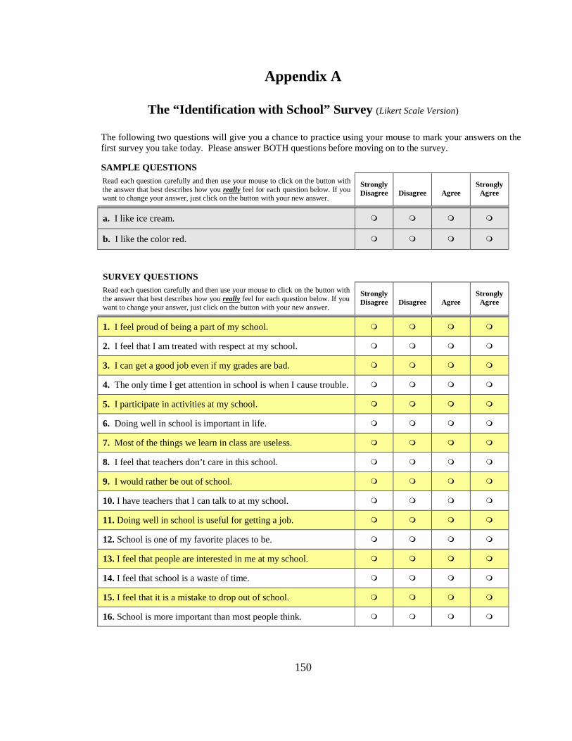
150
Appendix A
The “Identification with School” Survey (Likert Scale Version)
The following two questions will give you a chance to practice using your mouse to mark your answers on the first survey you take today. Please answer BOTH questions before moving on to the survey.
SAMPLE QUESTIONS Read each question carefully and then use your mouse to click on the button with the answer that best describes how you really feel for each question below. If you want to change your answer, just click on the button with your new answer.
Strongly Disagree
Disagree
Agree
Strongly Agree
a. I like ice cream. � � � �
b. I like the color red. � � � �
SURVEY QUESTIONS
Read each question carefully and then use your mouse to click on the button with the answer that best describes how you really feel for each question below. If you want to change your answer, just click on the button with your new answer.
Strongly Disagree
Disagree
Agree
Strongly Agree
1. I feel proud of being a part of my school. � � � �
2. I feel that I am treated with respect at my school. � � � �
3. I can get a good job even if my grades are bad. � � � �
4. The only time I get attention in school is when I cause trouble. � � � �
5. I participate in activities at my school. � � � �
6. Doing well in school is important in life. � � � �
7. Most of the things we learn in class are useless. � � � �
8. I feel that teachers don’t care in this school. � � � �
9. I would rather be out of school. � � � �
10. I have teachers that I can talk to at my school. � � � �
11. Doing well in school is useful for getting a job. � � � �
12. School is one of my favorite places to be. � � � �
13. I feel that people are interested in me at my school. � � � �
14. I feel that school is a waste of time. � � � �
15. I feel that it is a mistake to drop out of school. � � � �
16. School is more important than most people think. � � � �
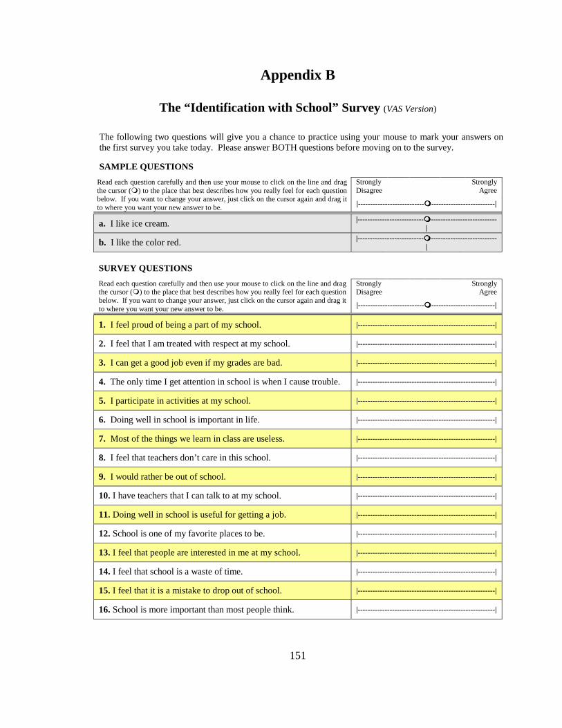
151
Appendix B
The “Identification with School” Survey (VAS Version)
The following two questions will give you a chance to practice using your mouse to mark your answers on the first survey you take today. Please answer BOTH questions before moving on to the survey.
SAMPLE QUESTIONS
Read each question carefully and then use your mouse to click on the line and drag the cursor (�) to the place that best describes how you really feel for each question below. If you want to change your answer, just click on the cursor again and drag it to where you want your new answer to be.
Strongly Disagree
Strongly Agree
|---------------------------����--------------------------|
a. I like ice cream. |---------------------------����---------------------------|
b. I like the color red. |---------------------------����---------------------------|
SURVEY QUESTIONS
Read each question carefully and then use your mouse to click on the line and drag the cursor (�) to the place that best describes how you really feel for each question below. If you want to change your answer, just click on the cursor again and drag it to where you want your new answer to be.
Strongly Disagree
Strongly Agree
|---------------------------����--------------------------|
1. I feel proud of being a part of my school. |--------------------------------------------------------|
2. I feel that I am treated with respect at my school. |--------------------------------------------------------|
3. I can get a good job even if my grades are bad. |--------------------------------------------------------|
4. The only time I get attention in school is when I cause trouble. |--------------------------------------------------------|
5. I participate in activities at my school. |--------------------------------------------------------|
6. Doing well in school is important in life. |--------------------------------------------------------|
7. Most of the things we learn in class are useless. |--------------------------------------------------------|
8. I feel that teachers don’t care in this school. |--------------------------------------------------------|
9. I would rather be out of school. |--------------------------------------------------------|
10. I have teachers that I can talk to at my school. |--------------------------------------------------------|
11. Doing well in school is useful for getting a job. |--------------------------------------------------------|
12. School is one of my favorite places to be. |--------------------------------------------------------|
13. I feel that people are interested in me at my school. |--------------------------------------------------------|
14. I feel that school is a waste of time. |--------------------------------------------------------|
15. I feel that it is a mistake to drop out of school. |--------------------------------------------------------|
16. School is more important than most people think. |--------------------------------------------------------|
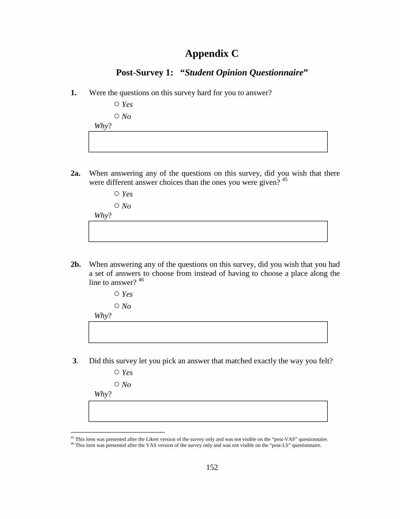
152
Appendix C
Post-Survey 1: “Student Opinion Questionnaire”
1. Were the questions on this survey hard for you to answer?
○ Yes
○ No Why?
2a. When answering any of the questions on this survey, did you wish that there were different answer choices than the ones you were given? 45
○ Yes
○ No Why?
2b. When answering any of the questions on this survey, did you wish that you had a set of answers to choose from instead of having to choose a place along the line to answer? 46
○ Yes
○ No Why? 3. Did this survey let you pick an answer that matched exactly the way you felt?
○ Yes
○ No Why?
45 This item was presented after the Likert version of the survey only and was not visible on the “post-VAS” questionnaire. 46 This item was presented after the VAS version of the survey only and was not visible on the “post-LS” questionnaire.

153
Appendix D
Post-Survey 2: “Student Demographic Questionnaire”
1. Think about the survey you just took. Which way did you like better for answering the questions?
○ I liked answering questions better when I had the four answers to choose from (like the example below).
[EXAMPLE] Strongly Disagree Disagree Agree
Strongly Agree
� � � �
○ I liked answering questions better when I had the line to click on to choose my answer (like the example below).
[EXAMPLE] Strongly Disagree
Strongly Agree
|---------------------------����----------------------------|
2. Are you a boy or a girl?
○ Boy
○ Girl
○ I prefer not to respond
3. What grade are you in? [drop-down menu] [1st, 2nd, 3rd, 4th, 5th, 6th, 7th, 8th, 9th, 10th, 11th, 12th, Other]
4. How old are you? [drop-down menu] [5, 6, 7, 8, 9, 10, 11, 12, 13, 14, 15, 16, 17, 18, 19 or Older]
5. Is English your first language?
○ Yes
○ No
6. Do you like your school?
○ Yes
○ No
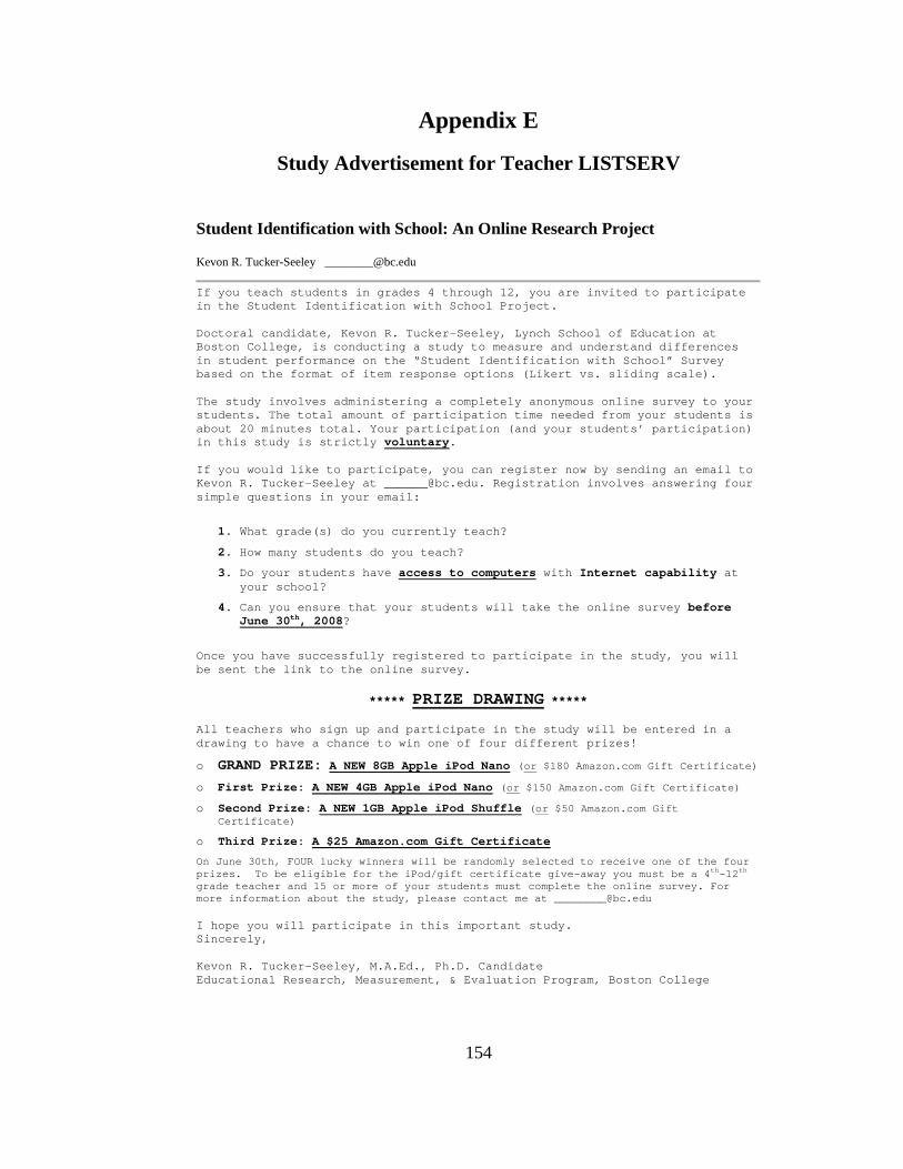
154
Appendix E
Study Advertisement for Teacher LISTSERV
Student Identification with School: An Online Research Project
Kevon R. Tucker-Seeley [email protected]
If you teach students in grades 4 through 12, you a re invited to participate in the Student Identification with School Project. Doctoral candidate, Kevon R. Tucker-Seeley, Lynch S chool of Education at Boston College, is conducting a study to measure an d understand differences in student performance on the “Student Identificati on with School” Survey based on the format of item response options (Liker t vs. sliding scale). The study involves administering a completely anony mous online survey to your students. The total amount of participation time ne eded from your students is about 20 minutes total. Your participation (and you r students’ participation) in this study is strictly voluntary. If you would like to participate, you can register now by sending an email to Kevon R. Tucker-Seeley at [email protected]. Registrati on involves answering four simple questions in your email:
1. What grade(s) do you currently teach?
2. How many students do you teach?
3. Do your students have access to computers with Internet capability at your school?
4. Can you ensure that your students will take the onl ine survey before June 30th, 2008?
Once you have successfully registered to participat e in the study, you will be sent the link to the online survey.
***** PRIZE DRAWING *****
All teachers who sign up and participate in the stu dy will be entered in a drawing to have a chance to win one of four differe nt prizes!
o GRAND PRIZE: A NEW 8GB Apple iPod Nano (or $180 Amazon.com Gift Certificate)
o First Prize: A NEW 4GB Apple iPod Nano (or $150 Amazon.com Gift Certificate)
o Second Prize: A NEW 1GB Apple iPod Shuffle (or $50 Amazon.com Gift Certificate)
o Third Prize: A $25 Amazon.com Gift Certificate
On June 30th, FOUR lucky winners will be randomly s elected to receive one of the four prizes. To be eligible for the iPod/gift certifica te give-away you must be a 4 th -12 th grade teacher and 15 or more of your students must complete the online survey. For more information about the study, please contact me at [email protected] I hope you will participate in this important study . Sincerely, Kevon R. Tucker-Seeley, M.A.Ed., Ph.D. Candidate Educational Research, Measurement, & Evaluation Pro gram, Boston College

155
Appendix F
Screen Shot: Identification with School Survey Student Assent Form
You are invited to take an online survey that will ask you questions about being a student at your school. Before you begin, you will be
asked to answer a few brief questions that will help you learn how to
respond to the survey. After you answer those, you will be able to take
today’s survey.
Statement of Consent:
YesI will participant in the study.
NoI do not w ish to participate in the study.
156
Appendix G
Screen Shot: Identification with School Survey “Welcome” and “Thank you” Message
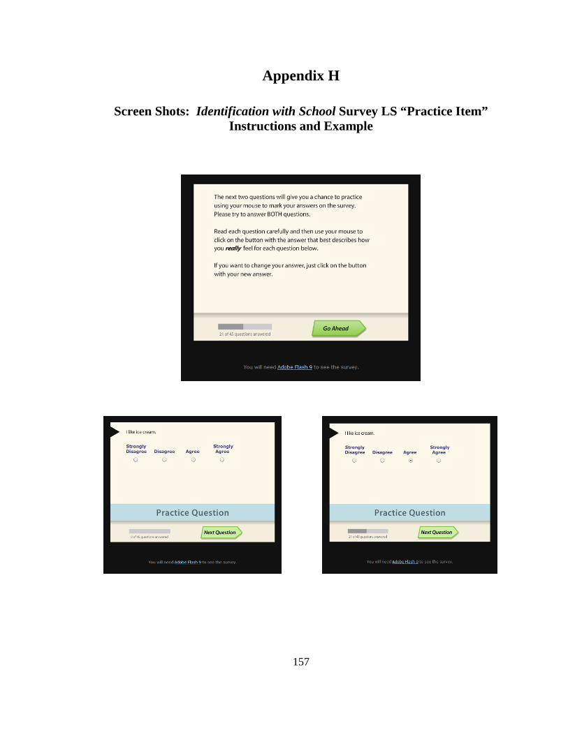
157
Appendix H
Screen Shots: Identification with School Survey LS “Practice Item” Instructions and Example

158
Appendix I
Screen Shots: Identification with School Survey VAS “Practice Item” Instructions and Example

159
Appendix J
Screen Shots: Identification with School Survey LS and VAS Item Examples
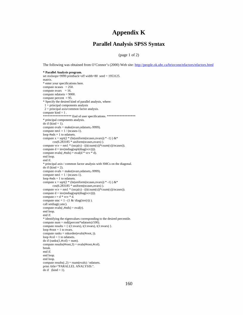
160
Appendix K
Parallel Analysis SPSS Syntax
(page 1 of 2) The following was obtained from O’Connor’s (2000) Web site: http://people.ok.ubc.ca/brioconn/nfactors/nfactors.html * Parallel Analysis program. set mxloops=9999 printback=off width=80 seed = 1953125. matrix. * enter your specifications here. compute ncases = 250. compute nvars = 16. compute ndatsets = 9000. compute percent = 95. * Specify the desired kind of parallel analysis, where: 1 = principal components analysis 2 = principal axis/common factor analysis. compute kind = 1 . ****************** End of user specifications. **** ************** * principal components analysis. do if (kind = 1). compute evals = make(nvars,ndatsets,-9999). compute nm1 = 1 / (ncases-1). loop #nds = 1 to ndatsets. compute x = sqrt(2 * (ln(uniform(ncases,nvars)) * -1) ) &* cos(6.283185 * uniform(ncases,nvars) ). compute vcv = nm1 * (sscp(x) - ((t(csum(x))*csum(x))/ncases)). compute d = inv(mdiag(sqrt(diag(vcv)))). compute evals(:,#nds) = eval(d * vcv * d). end loop. end if. * principal axis / common factor analysis with SMCs on the diagonal. do if (kind = 2). compute evals = make(nvars,ndatsets,-9999). compute nm1 = 1 / (ncases-1). loop #nds = 1 to ndatsets. compute x = sqrt(2 * (ln(uniform(ncases,nvars)) * -1) ) &* cos(6.283185 * uniform(ncases,nvars) ). compute vcv = nm1 * (sscp(x) - ((t(csum(x))*csum(x))/ncases)). compute d = inv(mdiag(sqrt(diag(vcv)))). compute r = d * vcv * d. compute smc = 1 - (1 &/ diag(inv(r)) ). call setdiag(r,smc). compute evals(:,#nds) = eval(r). end loop. end if. * identifying the eigenvalues corresponding to the desired percentile. compute num = rnd((percent*ndatsets)/100). compute results = { t(1:nvars), t(1:nvars), t(1:nvars) }. loop #root = 1 to nvars. compute ranks = rnkorder(evals(#root,:)). loop #col = 1 to ndatsets. do if (ranks(1,#col) = num). compute results(#root,3) = evals(#root,#col). break. end if. end loop. end loop. compute results(:,2) = rsum(evals) / ndatsets. print /title="PARALLEL ANALYSIS:". do if (kind = 1).

161
(page 2 of 2) print /title="Principal Components". else if (kind = 2). print /title="Principal Axis / Common Factor Analysis". end if. compute specifs = {ncases; nvars; ndatsets; percent}. print specifs /title="Specifications for this Run:" /rlabels="Ncases" "Nvars" "Ndatsets" "Percent". print results /title="Random Data Eigenvalues" /clabels="Root" "Means" "Prcntyle" /format "f12.6". do if (kind = 2). print / space = 1. print /title="Compare the random data eigenvalues to the". print /title="real-data eigenvalues that are obtained from a". print /title="Common Factor Analysis in which the # of factors". print /title="extracted equals the # of variables/items, and the". print /title="number of iterations is fixed at zero;". print /title="To obtain these real-data values using SPSS, see the". print /title="sample commands at the end of the parallel.sps program,". print /title="or use the rawpar.sps program.". print / space = 1. print /title="Warning: Parallel analyses of adjusted correlation matrices". print /title="eg, with SMCs on the diagonal, tend to indicate more factors". print /title="than warranted (Buja, A., & Eyuboglu, N., 1992, Remarks on parallel". print /title="analysis. Multivariate Behavioral Research, 27, 509-540.).". print /title="The eigenvalues for trivial, negligible factors in the real". print /title="data commonly surpass corresponding random data eigenvalues". print /title="for the same roots. The eigenvalues from parallel analyses". print /title="can be used to determine the real data eigenvalues that are". print /title="beyond chance, but additional procedures should then be used". print /title="to trim trivial factors.". print / space = 1. print /title="Principal components eigenvalues are often used to determine". print /title="the number of common factors. This is the default in most". print /title="statistical software packages, and it is the primary practice". print /title="in the literature. It is also the method used by many factor". print /title="analysis experts, including Cattell, who often examined". print /title="principal components eigenvalues in his scree plots to determine". print /title="the number of common factors. But others believe this common". print /title="practice is wrong. Principal components eigenvalues are based". print /title="on all of the variance in correlation matrices, including both". print /title="the variance that is shared among variables and the variances". print /title="that are unique to the variables. In contrast, principal". print /title="axis eigenvalues are based solely on the shared variance". print /title="among the variables. The two procedures are qualitatively". print /title="different. Some therefore claim that the eigenvalues from one". print /title="extraction method should not be used to determine". print /title="the number of factors for the other extraction method.". print /title="The issue remains neglected and unsettled.". end if. end matrix. * Commands for obtaining the necessary real-data eigenvalues for principal axis / common factor analysis using SPSS; make sure to insert valid filenames/locations, and remove the '*' from the first columns. * corr var1 to var20 / matrix out ('filename') / missing = listwise. * matrix. * MGET /type= corr /file='filename' . * compute smc = 1 - (1 &/ diag(inv(cr)) ). * call setdiag(cr,smc). * compute evals = eval(cr). * print { t(1:nrow(cr)) , evals } /title="Raw Data Eigenvalues" /clabels="Root" "Eigen." /format "f12.6". * end matrix.