Analysing Ewald’s Method for the Evaluation of Green’s ...schmitt/media/ewald-periodic.pdf · Analysing Ewald’s Method for the Evaluation of Green’s Functions for Periodic

IMA Journal of Numerical Analysis(2010) Page 1 of 25doi:10.1093/imanum/drn000

Analysing Ewald’s Method for the Evaluation of Green’s Functions forPeriodic Media

TILO ARENS†, KAI SANDFORT‡, SUSANNE SCHMITT§

Karlsruhe Institute of Technology (KIT), 76128 Karlsruhe,Germany

andARMIN LECHLEITER¶

INRIA Saclay, Ecole Polytechnique, Route de Saclay, 91128 Palaiseau, France

[Received on : manuscript submitted for publication]

Expressions for periodic Green’s functions for the Helmholtz equation in two and three dimensions arederived via Ewald’s method. The decay rate of the series occurring in these expressions is analysedand rigorous estimates for the remainder are derived when the series are truncated and replaced by finitesums. The effect of choosing a control parameter occurring in Ewald’s expressions is discussed and somerecommendations for its choice are given based on the aforementioned estimates. We present variousnumerical examples for the resulting method for evaluatingthe Green’s functions. The results can alsobe carried over to evaluating the partial derivatives.

Keywords: keywords

1. Introduction

In this article, we carry out a theoretical and numerical analysis of the so-called Ewald’s representationof the periodic and biperiodic Green’s functions for the Helmholtz equation in two and three spatialdimensions. There are applications for these functions from which integral equation formulations forscattering problems are of particular interest to the authors (Arens, 2010; Sandfort, 2010). The needto evaluate the Green’s function and its derivatives is often a limiting factor in these approaches. Forthe Helmholtz operator and the free-space or half-space geometry, there are simple expressions for theGreen’s functions which can easily be evaluated. For more complicated geometries, including periodicmedia, the Green’s functions are usually given formally by series expansions which might be onlyslowly convergent or even divergent depending on the valuesof the problem parameters. However, toimplement efficient numerical schemes for solving the boundary integral equations, it is essential tohave representations of the Green’s functions available which allow the fast and accurate evaluation forall admissible problem parameters.

In the review article (Linton, 1998), a number of analyticaltechniques to derive such convenientexpressions for the Green’s function for the two-dimensional Helmholtz equation in periodic domainsare discussed and compared in-depth. One of the best-performing methods presented is Ewald’s trans-formation. This transformation was originally derived in (Ewald, 1921) for the computation of three-dimensional lattice potentials. It splits the series representation of the lattice potential, and likewise that

†Corresponding author. Email: [email protected]‡Email: [email protected]§Email: [email protected]¶Email: [email protected]

c© The author 2010. Published by Oxford University Press on behalf of the Institute of Mathematics and its Applications. All rights reserved.

2 of 25 ARENSET AL.

of the periodic Green’s function, into a sum of two series, oftypes different from that of the originalseries, which are both exponentially convergent. From the big amount of alternative methods, besidesthe references given in (Linton, 1998), we also mention (Sadov, 1997) and (Kurkcu & Reitich, 2009).

Ewald’s method became commonly used in the physics community and is covered predominantlyin the engineering and physics literature, though it is attractive not only from the numerical, but alsothe theoretical point of view. In addition to the two-dimensional quasi-periodic Green’s function asdiscussed in (Linton, 1998) and references given therein, expressions for the three-dimensional quasi-biperiodic Green’s function were also derived (Kambe, 1967). However, this function has not been dis-cussed much further in the literature. For the two-dimensional quasi-periodic Green’s function, Ewald’sapproach has been discussed in a number of articles, e.g. (Jordanet al., 1986) and (Capolinoet al.,2005). In all cases known to the authors, asymptotical behaviour of the terms in the series is discussedand conclusions are backed by some numerical examples.

The present paper contributes to this subject firstly by giving, in Section 3, a detailed and rigorousderivation of the Ewald representation for the two-dimensional quasi-periodic Green’s function for theHelmholtz equation, clearly separating technicalities from core arguments. A companion analysis alongsimilar lines for the three-dimensional bi-quasi-periodic Green’s function is contained in (Arens, 2010).

Secondly, and this is the main novel contribution, we give inSections 4 and 5 rigorous and com-putable error bounds for truncated versions of the series both for the two- and the three-dimensionalcases. Provided that cancellation effects do not play a dominant role, these estimates allow the evalua-tion of the Green’s functions to a prescribed error.

A further aspect of Ewald’s method is that it involves a parameter that can be used to influence thespeed of convergence of all series. Various authors give recommendations for choosing this parameter(Jordanet al., 1986; Mathis & Peterson, 1996; Kustepeli & Martin, 2000; Capolino et al., 2005). Therule of thumb appears to be to choose a constant parameter that gives good numerical accuracy reliably.However, an optimal choice should minimise the total effortfor the evaluation for a prescribed accuracy.We propose an algorithm that chooses this parameter automatically while guaranteeing optimality insome sense. As a bad choice of the control parameter will alsolead to cancellation and instability,conditions are formulated that prevent this case. For the two-dimensional case, the only similar workin this respect appears to be (Capolinoet al., 2005) and our results for the 2D case in this respect onlydiffer in details. For the three-dimensional case, our results appear to be completely new. A number ofnumerical examples illustrate the performance of the proposed methods. The computations were carriedout using the program librarylibewald written by the authors in the programming languageC. Thesource code of this library, which contains programs to produce all results presented in this paper, isavailable athttp://libewald.sourceforge.net.

In many applications, including boundary integral equation methods, not only the Green’s function,but also its gradient is required. Therefore, in Section 7 westudy the gradient of the Ewald’s represen-tation and corresponding error estimates. Some numerical results are also given.

2. Periodic Green’s Functions

The propagation of time-harmonic acoustic waves with wave numberk> 0 is modelled by the Helmholtzequation

∆u+k2u = 0. (2.1)

ANALYSING EWALD’S METHOD 3 of 25

Absorption in the medium can be taken into account by allowing wave numbers with arg(k) ∈ [0,π/2).The fundamental solution, or Green’s function in free-fieldconditions, of (2.1) is given by

Φ(x,y) =i4

H(1)0 (k|x−y|), x,y∈ R

2, x 6= y, (2.2)

in two spatial dimensions, whereH(1)ν is the Hankel function of the first kind and of orderν, and by

Φ(x,y) =1

4πeik|x−y|

|x−y| , x,y∈ R3, x 6= y, (2.3)

in three spatial dimensions. Note that through

eikr

r=

√

kπ2r

H(1)−1/2(kr), r > 0, (2.4)

both fundamental solutions can be expressed via a Hankel function of the first kind.Consider now a domainΩ ⊆ R2 which isL-periodic,L > 0, in thex1-direction, i.e. forx∈ Ω there

holds(x1 + µL,x2)⊤ ∈ Ω for all µ ∈ Z. If (2.1) is considered in such a domain, it is usual to consider

α-quasi-periodic fields for someα ∈ R. Such fields areL-periodic up to a phase shift,

u(x1 +L,x2) = eiLα u(x1,x2), x∈ Ω .

A typical example of such a field is a plane waveu(x) = exp(ikd · x) with d a unit vector, which iskd1-quasi-periodic.

In scattering problems for suchL-periodic media, one considers theα-quasi-periodic Green’s func-tion for the Helmholtz equationGq2. One possible expression for this function is a series of translatedpoint sources,

Gq2(x−y) =i4 ∑

µ∈Z

eiµαL H(1)0

(

k

∣

∣

∣

∣

x−y− µ(

L0

)∣

∣

∣

∣

)

, (2.5)

wherex, y ∈ R2 such thatx− y 6= µ (L,0)⊤ for all µ ∈ Z. Convergence of the series in (2.5) can beestablished from asymptotic decay rates of Hankel functions in the cases where

Im(k) > 0 or

[

k > 0 and α +2πL

µ 6= k for all µ ∈ Z

]

(2.6)

is satisfied (see e.g. (Arens, 1999) for explicit calculations). For realk, the terms in (2.5) decay as|µ |−1/2 so that convergence is rather slow and the series certainly does not converge absolutely. A fasterconverging representation of this Green’s function is desirable for numerical purposes.

A further expression can be obtained by computing the expansion of Gq2 in trigonometric polyno-mials. We set

αµ =α +2πµ/L

kand βµ =

√

1−α2µ , µ ∈ Z,

where the square root function is analytically continued tothe complex plane except for a branch cutalong the negative imaginary axis. Then the Fourier series expansion ofGq2 is given by

Gq2(x−y) =i

2kL ∑µ∈Z

1βµ

eik[αµ (x1−y1)+βµ |x2−y2|], (2.7)

4 of 25 ARENSET AL.

again forx, y∈ R2 such thatx−y 6= µ (L,0)⊤ for anyµ ∈ Z. Expression (2.7) is exponentially conver-gent wheneverx2 6= y2. However, for realk andx2 = y2 we observe a decay of|µ |−1 of the terms inthe series so convergence is again slow. Also, if 2π/(kL) is small,βµ will be real for a large range ofµ and the growth of its absolute value relatively slow outsidethis range so that many terms in (2.7) arerequired for an accurate numerical evaluation ofGq2.

The second Green’s function under consideration is the three-dimensional analogue ofGq2. Weconsider a domainΩ ⊆R3 which is assumed to beL1-periodic in thex1-direction andL2-periodic in thex2-direction. For ease of notation, we define the lattice translation vectorsp(µ) and the reciprocal latticevectorsq(µ) by

p(µ) =

µ1L1

µ2L2

0

and q(µ) =

µ12π/L1

µ22π/L2

0

, µ ∈ Z2,

respectively. Similarly as for the two-dimensional case, we call a fieldu α-quasi-biperiodic for someα ∈ R3, α3 = 0, if

u(x+ p(µ)) = eiα ·p(µ)u(x), x∈ Ω , µ ∈ Z

2.

Theα-quasi-biperiodic Green’s function can be expressed formally as (Arens, 2010; Kambe, 1967)

Gq3(x−y) =1

4π ∑µ∈Z2

eiα ·p(µ) eik|x−y−p(µ)|

|x−y− p(µ)| (2.8)

for x, y∈ Ω such thatx−y 6= p(µ) for anyµ ∈ Z2. Setting

α(µ) =α +q(µ)

kand ρµ =

√

1−|α(µ)|2, µ ∈ Z2,

an expansion in trigonometric polynomials with respect to bothx1 andx2 gives

Gq3(x−y) =i

2kL1L2∑

µ∈Z2

1ρµ

eik[α(µ)·(x−y)+ρµ |x3−y3|]. (2.9)

Here, and in all further arguments, we denote forx∈ R3 by x the projection onto thex1,x2)-plane, i.e.x = (x1,x2,0)⊤.

For such two-dimensional lattice sums, absolute convergence is required to make the expressionwell-defined. In (2.8), this is the case for Im(k) > 0, but not for a real wave number. The expression (2.9)is absolutely convergent even for realk, butx3 6= y3 is required. Hence, in the case of a biperiodic grating,an alternative exponentially convergent representation of the Green’s function is not only desirable fornumerical but also for analytical purposes.

3. Ewald’s Method

The principle of Ewald’s method for the derivation of quickly convergent representations of periodicGreen’s functions is rather simple. We heuristically present the idea for a function periodic in onedirection. Consider a functionf : Ω → C which has a singularity at 0 and which is slowly decaying forlarge arguments. Next, we define theL-periodic function

F(x) = ∑µ∈Z

f (x+ µLe1), x∈ Ω ,


wheree1 is the first coordinate unit vector. Of course,Ω is assumed to be a domain such thatx+µLe1 ∈Ω for all x∈ Ω and allµ ∈ Z.

For both the Green’s functions considered in Section 2, a respective f will somehow involve aHankel function. As will be shown below, we may split a Hankelfunction into a singular but quicklydecaying and a smooth but slowly decaying function. In otherwords, we writef = g+( f −g), whereg has the same singularity at 0 asf and is exponentially decaying for large arguments, to obtain

F(x) = ∑µ∈Z

g(x+ µLe1)+ ∑µ∈Z

( f (x+ µLe1)−g(x+ µLe1)) , x∈ Ω .

The second sum in this expression may be rewritten by means ofthe so-calledPoisson summationformula,which yields

F(x) = ∑µ∈Z

g(x+ µLe1)+1L ∑

µ∈Z

[

f

(

2πµL

,Px

)

− g

(

2πµL

,Px

)]

ei(2πµ/L)x1, (3.1)

for x∈ Ω , wherePx denotes the orthogonal projection ofx onto the orthogonal complement ofe1 andf denotes the one-dimensional Fourier transform in the direction of p,

f (ξ ,z) =

∫ ∞

−∞f (z+ ηe1)e−iξ η dη , ξ ∈ R, z∈ (spane1)⊥.

Now, both series appearing in (3.1) are quickly convergent:the functiong is exponentially decreasingitself while f −g is smooth and hence its Fourier transform is quickly decaying for large argument.

Let us first work out the necessary expressions forGq2 in detail. For the derivation, we will assumethatarg(k) ∈ (0,π/2). In the final result, it is then possible to carry out the limitIm(k) → 0, so that therepresentation of the Green’s function we obtain is valid for realk as well.

As shown in detail in (Arens, 2010), though the result can be found in various places in the litera-ture, from standard expressions for Bessel function one mayderive the following representation for theHankel function of the first kind and of orderν ∈ R,

H(1)ν (kx) =

2i π

e−iπν(

k2x

)ν ∫

γ1

t−2ν−1 exp

(

−x2t2 +k2

4t2

)

dt ,

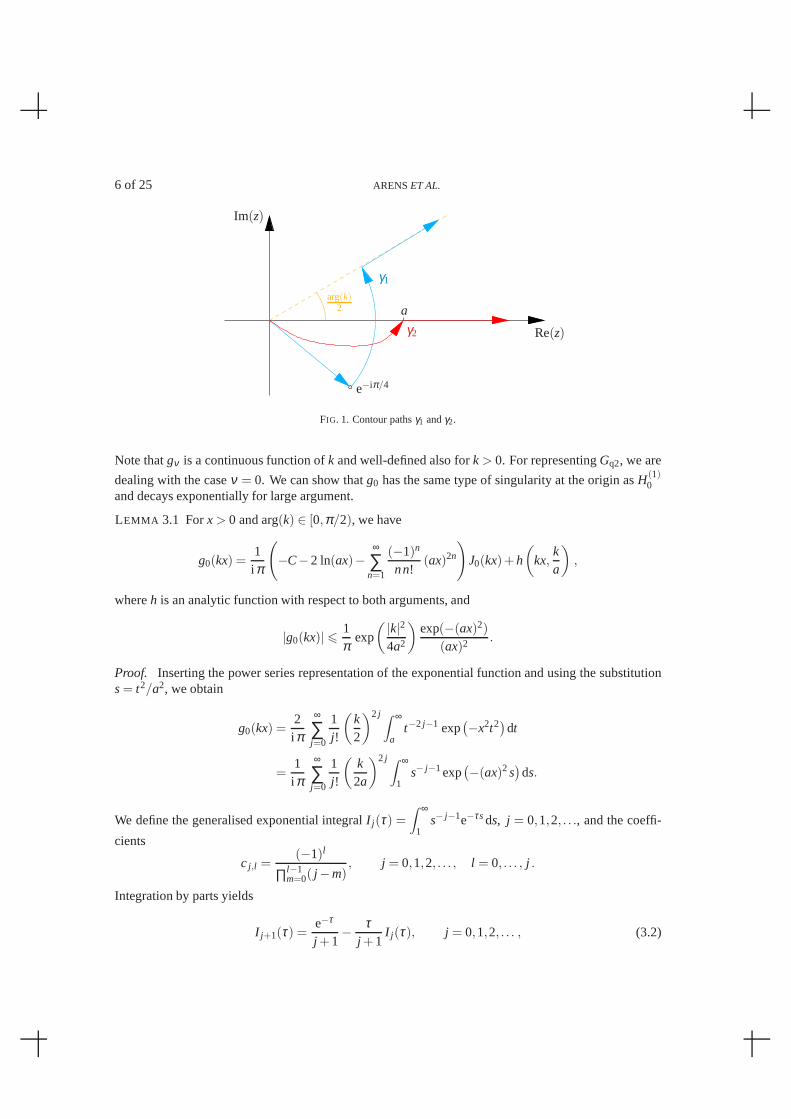
wherex> 0 and arg(k)∈ (0,π/2). Furthermore,γ1 denotes an integration path in the complex plane thatstarts at the origin in the direction e−iπ/4 and approaches infinity in the direction ei arg(k)/2, see Figure 1.

The path of integration may deviate fromγ1 as long as two conditions are met: The direction atwhich the path leaves the origin must not change and the path must go to infinity at a direction eiϕ with−π/4 < ϕ < π/4. This ensures Re(t2) > 0 so that the integrand decays exponentially for|t| → ∞. Forν > −1/2, we may even pass to the limitϕ →−π/4, in which case the integral exists as an improperintegral.

For the application of Ewald’s method, we use a path that connects the origin with a pointa > 0 andthen continues to infinity along the positive real axis. Thisintegration contour is shown in Figure 1 asγ2.

Let us define the function obtained by an integration along that section ofγ2 which coincides withthe real axis,

gν(kx) =2i π

e−iπν(

k2x

)ν ∫ ∞

at−2ν−1 exp

(

−x2t2 +k2

4t2

)

dt.

6 of 25 ARENSET AL.

e−iπ/4

γ1

γ2

arg(k)2 a

Im(z)

Re(z)

FIG. 1. Contour pathsγ1 andγ2.

Note thatgν is a continuous function ofk and well-defined also fork > 0. For representingGq2, we are

dealing with the caseν = 0. We can show thatg0 has the same type of singularity at the origin asH(1)0

and decays exponentially for large argument.

LEMMA 3.1 Forx > 0 and arg(k) ∈ [0,π/2), we have

g0(kx) =1i π

(

−C−2 ln(ax)−∞

∑n=1

(−1)n

nn!(ax)2n

)

J0(kx)+h

(

kx,ka

)

,

whereh is an analytic function with respect to both arguments, and

|g0(kx)| 6 1π

exp

( |k|24a2

)

exp(−(ax)2)

(ax)2 .

Proof. Inserting the power series representation of the exponential function and using the substitutions= t2/a2, we obtain

g0(kx) =2i π

∞

∑j=0

1j!

(

k2

)2 j ∫ ∞

at−2 j−1 exp

(

−x2t2)dt

=1i π

∞

∑j=0

1j!

(

k2a

)2 j ∫ ∞

1s− j−1exp

(

−(ax)2s)

ds.

We define the generalised exponential integralI j(τ) =

∫ ∞

1s− j−1e−τsds, j = 0,1,2, . . ., and the coeffi-

cients

c j ,l =(−1)l

∏l−1m=0( j −m)

, j = 0,1,2, . . . , l = 0, . . . , j .

Integration by parts yields

I j+1(τ) =e−τ

j +1− τ

j +1I j(τ), j = 0,1,2, . . . , (3.2)


and a simple induction argument leads to the explicit formula

I j(τ) = c j , j τ j I0(τ)−(

j

∑l=1

c j ,l τ l−1

)

e−τ , j = 0,1,2, . . .

Hence

g0(kx) =1i π

[

I0((ax)2)∞

∑j=0

c j , j

j!

(

kx2

)2 j

−e−(ax)2∞

∑j=0

j

∑l=1

c j ,l

j!

(

k2a

)2 j

(ax)2(l−1)

]

,

which we rewrite slightly as

g0(kx) =1i π

[

I0((ax)2)∞

∑j=0

c j , j

j!

(

kx2

)2 j

−e−(ax)2∞

∑l=0

(

kx2

)2l ∞

∑j=1

c j+l ,l+1

( j + l)!

(

k2a

)2 j]

.

Note thatc j , j = (−1) j/ j!, j = 0,1,2, . . ., so that we can substitute

∞

∑j=0

c j , j

j!

(

kx2

)2 j

=∞

∑j=0

(−1) j

( j!)2

(

kx2

)2 j

= J0(kx),

whereJ0 denotes the Bessel function of order 0 (see (Abramowitz & Stegun, 1965, formula 9.1.10)).For I0, we obtain from (Abramowitz & Stegun, 1965, formulae 5.1.1 and 5.1.12)

I0(τ) = E1(τ) = −C− lnτ −∞

∑n=1

(−1)n

nn!τn,

whereC is Euler’s constant andE1 denotes the exponential integral function. Hence

g0(kx) =1i π

[(

−C−2 ln(ax)−∞

∑n=1

(−1)n

nn!(ax)2n

)

J0(kx)

−e−(ax)2∞

∑l=0

(

kx2

)2l ∞

∑j=1

c j+l ,l+1

( j + l)!

(

k2a

)2 j]

,

which is the first part of the assertion.For j = 0,1,2, . . ., we can further estimate

∫ ∞

1s− j−1exp(−(ax)2s)ds6

∫ ∞

1exp(−(ax)2s)ds=

exp(−(ax)2)

(ax)2 .

Thus,

|g0(kx)| 6 1π

∞

∑j=0

1j!

∣

∣

∣

∣

k2a

∣

∣

∣

∣

2 j exp(−(ax)2)

(ax)2 =1π

exp

( |k|24a2

)

exp(−(ax)2)

(ax)2

and the proof is complete.

8 of 25 ARENSET AL.

We now start from (2.5) replacing the Hankel function byg0 and define forz∈ R2, z 6= 0,

F(1)q2 (z) =

i4 ∑

µ∈Z

eiµαL g0(k|z− µLe1|)),

= ∑µ∈Z

eiµαL

4π

∞

∑j=0

1j!

(

k2a

)2 j ∫ ∞

1s− j−1e−(a|z−µLe1|)2 sds. (3.3)

The heuristic arguments show a possibility to obtain a quickly convergent representation of

F (2)q2 (z) := Gq2(z)−F(1)

q2 (z). (3.4)

We set

h0(kx) = H(1)0 (kx)−g0(kx) =

2i π

∫

γ2

t−1 exp

(

−x2t2 +k2

4t2

)

dt,

whereγ2 denotes that part ofγ2 which is not the interval(a,∞). From the Fourier transform

∫ ∞

−∞exp(

−η2t2)exp(−iξ η)dη = e−ξ 2/(4t2)∫ ∞

−∞exp

(

−(

ηt +iξ2t

)2)

dη = e−ξ 2/(4t2)√

πt

,

where the last equality follows from an application of Cauchy’s integral theorem, we obtain∫ ∞

−∞h0(k|x|)e−ix1sdx1 =

2

i√

π

∫

γ4

t−2e−x22t2 exp

(

k2−s2

4t2

)

dt.

After compensating for the factor eiµαL, we can now apply Poisson’s summation formula to conclude

F (2)q2 (z) =

2i√

π L ∑µ∈Z

ei kαµ z1

∫

γ2

t−2e−(z2)2t2 exp

(

k2β 2µ

4t2

)

dt.

A further simplification of this expression can be achieved,starting from the substitutionu= 1/t. Settingγ3 = z∈ C : u = 1/t, t ∈ γ2 gives

F (2)q2 (z) =

2i√

π L ∑µ∈Z

ei kαµ z1

∫

γ3

exp

(

− z22

u2 +u2k2β 2

µ

4

)

du.

We have to distinguish cases depending on the sign of Re(k2β 2µ). Suppose first that Re(k2β 2

µ) < 0. Inthis case, the path of integration can be shifted to the interval (1/a,∞) and (Abramowitz & Stegun,1965, equation 7.4.33) yields

∫

γ3

e−z22u2 +

u2k2β2µ4 du =

i√

π2kβµ

(

e−i kβµ z2 erfc

(

az2− ikβµ

2a

)

+ei kβµ z2 erfc

(

−az2− ikβµ

2a

))

.

In the case Re(k2β 2µ) > 0 we perform another substitutions = −iu and then apply (Abramowitz &

Stegun, 1965, equation 7.4.33) to end up with the same result. The case Re(k2β 2µ) = 0 is obtained from

the other two by continuity. Concluding, we have obtained the expression

F (2)q2 (z) =

i4L ∑

µ∈Z

1kβµ

ei kαµ z1

(

e−i kβµ z2 erfc

(

az2− ikβµ

2a

)

+ei kβµ z2 erfc

(

−az2− ikβµ

2a

))


for the function defined in (3.4). It will be beneficial for subsequent arguments to write this function astwo separate series which differ only in the sign of some arguments,

F (2,±)q2 (z) =

i4L ∑

µ∈Z

1kβµ

ei kαµ z1 e∓i kβµ z2 erfc

(

±az2− ikβµ

2a

)

.

From Lemma 3.1, we see that the terms in the representation ofF(1)q2 are exponentially decaying. We

prove the same forF(2)q2 .

LEMMA 3.2 Chooseµ0 ∈ Z such that|kαµ0|6 |kαµ | for all µ ∈ Z. Then there existsM ∈ N dependentonk, α andz2 such that for allµ ∈ Z with |µ | > M,

∣

∣

∣

∣

e∓i kβµ0+µ z2 erfc

(

±az2− ikβµ0+µ

2a

)∣

∣

∣

∣

6 exp

( |k|24a2 −a2z2

2−π2

(aL)2 (|µ |−1)2)

.

Proof. The complementary error function can be expressed using theFaddeeva functionw (see

(Abramowitz & Stegun, 1965, Formula 7.1.3)). Thus, the terms in the expression forF (2)q2 can be written

as

e∓i kβµ z2 erfc

(

±az2− ikβµ

2a

)

= e−a2z2

2+(

kβµ2a

)2

w

(

±iaz2 +kβµ

2a

)

. (3.5)

If the absolute value ofµ is large enough, we have arg(±iaz2 + kβµ/(2a)) ∈ [0,π/2). For such argu-ments, the absolute value of the Faddeeva function is bounded by 1. Indeed, forx∈ R, y∈ R>0,

|w(x+ iy)|2 =4π

e−2x2+2y2∣

∣

∣

∣

2√π

∫ ∞

y−ixe−t2 dt

∣

∣

∣

∣

2

=4π

e−2x2+2y2∣

∣

∣

∣

∫ ∞

0e−(s+y−ix)2

ds

∣

∣

∣

∣

2

=4π

∣

∣

∣

∣

∫ ∞

0e−2s(y−ix)−s2

ds

∣

∣

∣

∣

2

=4π

∣

∣

∣

∣

∫ ∞

0

∫ ∞

0e−2(s+t)y+2i(s−t)x−s2−t2 dsdt

∣

∣

∣

∣

64π

∫ ∞

0

∫ ∞

0e−s2−t2 dsdt = 1.

We further have forµ ∈ Z\ 0 ands∈ −1,0,1(

α +2πL

(µ0 + µ)

)2

>4πL

(

α +2πL

(µ0 +s)

)

(µ −s)+4π2

L2 (µ −s)2

and hence(

α +2πL

(µ0 + µ)

)2

>4π2

L2 (|µ |−1)2 .

As

k2β 2µ+µ0

= k2−(

α +2πL

(µ0 + µ)

)2

,

combining the above estimate with (3.5) and the bound for theFaddeeva function yields the assertion.

The statements made in Lemmas 3.1 and 3.2 have been observed frequently in the literature, mostoften expressed using asymptotic formulae. Although theseestimates give the qualitative behaviourof the series obtained by Ewald’s method, they are not enough, however, to guarantee a given errortolerance in the numerical evaluation.

10 of 25 ARENSET AL.

4. Numerical Evaluation of the Ewald Representation

It is the pupose of this section to analyse the difference between the partial sums

F (1)q2,M(z) =

µ0+M

∑µ=µ0−M

eiµαL

4π

∞

∑j=0

1j!

(

k2a

)2 j ∫ ∞

1s− j−1e−(a|z−µLe1|)2 sds, (4.1)

F (2,±)q2,M (z) =

i4L

µ0+M

∑µ=µ0−M

1kβµ

ei kαµ z1 e∓i kβµ z2 erfc

(

±az2− ikβµ

2a

)

, (4.2)

and the full series, respectively, and to discuss the computation of numeric values for these series. Theparameterµ0 should be chosen to center the corresponding partial sum on the dominating terms in theseries. Our results below will include reasonable choices.

We first address the series remaining in (4.1). Defining

F(1)aux(R,κ ,ν) =

∞

∑j=0

1j!

κ j∫ ∞

1s− j−νe−Rsds.

the first function can be rewritten as

F (1)q2,M(z) =

M

∑µ=−M

eiµαL

4πF (1)

aux

(

a2|z− µLe1|2,(

k2a

)2

,1

)

.

For most of the remaining discussion we will assume that we can evaluateF (1)aux exactly, just as any other

standard or special function used in our expressions. However, the following lemma gives us someessential properties of this function.

LEMMA 4.1 ForR> 0, arg(κ) ∈ [0,π/2) andν > 0 we have∣

∣

∣F(1)aux(R,κ ,ν)

∣

∣

∣6exp(|κ |−R)

R,

and additionally for allM ∈ N, ν > 0,∣

∣

∣

∣

∣

F (1)aux(R,κ ,ν)−

M

∑j=0

1j!

κ j∫ ∞

1s− j−νe−Rsds

∣

∣

∣

∣

∣

6e|κ |−R

M + ν

( |κ |M +1

)M+1

.

Proof. The first estimate is elementary. The estimate for the remainder can be obtained from the

observation that the integral in the expression forF (1)aux is equal to a generalised exponential integral.

From (Hopf, 1934, page 26) we obtain

e−R

R+ p<

∫ ∞

1s−pe−Rsds6

e−R

R+ p−1, R, p > 0.

Hence∣

∣

∣

∣

∣

∞

∑j=M+1

1j!

κ j∫ ∞


∣

∣

∣

∣

∣

6e−R

R+M + ν

∞

∑j=M+1

1j!|κ | j 6

e|κ |−R

M + ν

( |κ |M +1

)M+1

.

It is now fairly simple to estimate the remainder forF (1)q2 .


THEOREM 4.1 Defineµ0 ∈ Z by z1− µ0L ∈ (−L/2,L/2] and letM ∈ N. Then

∣

∣

∣F (1)

q2 (z)−F(1)q2,M(z)

∣

∣

∣6

exp(

|k|2/(4a2)−a2z22

)

2π a2(

z22 +(ML)2

)

(1−exp(−2a2ML2))e−(aML)2

.

Proof. From the first estimate in Lemma 4.1 we have

∣

∣

∣F(1)q2 (z)−F(1)

q2,M(z)∣

∣

∣61

4π ∑|µ−µ0|>M+1

∣

∣

∣

∣

∣

F(1)aux

(

a2((z1− µL)2 +z22

)

,

(

k2a

)2

,1

)∣

∣

∣

∣

∣

6exp(

|k2|/(4a2)−a2z22

)

4π ∑|µ−µ0|>M+1

exp(

−a2(z1− µL)2)

a2(

(z1− µL)2 +z22

) .

For |µ − µ0| > M +1, we find

(z1− µL)2 > (z1− µ0L± (M +1)L)2+2L(z1− µ0± (M +1)L)(µ0− µ ∓ (M +1)),

from which we conclude

(z1− µL)2> M2L2 +2ML2 (|µ0− µ |− (M +1)) > M2L2 .

Thus

∑|µ−µ0|>M+1

exp(

−a2(z1− µL)2)

a2((z1− µL)2 +z22)

62 exp(−(aML)2)

a2(

(ML)2 +z22

)

∞

∑µ=M+1

e−2ML2a2(µ−(M+1)) .

The assertion now follows using the geometric series.

The analysis of the two functions representingF(2)q2 is slightly more complicated. One way to eval-

uate the complementary error function is through (3.5) using the Faddeeva function. However, in thecase±az2+ Im(kβµ/(2a)) < 0 a numerical evaluation of the right-hand side of (3.5) may not be stable.In this case, we use the elementary formula

w(z) = w(−z) = 2e−z2 −w(z)

to obtain

e−i kβµ z2 erfc

(

az2− ikβµ

2a

)

= 2e−i kβµ z2 −e−a2z2

2+(

kβµ2a

)2

w

(

−iaz2 +kβµ

2a

)

. (4.3)

The representations (3.5) and (4.3) also lead to separate error estimates valid for different ranges ofcut-off indices.

THEOREM 4.2 Chooseµ0 as in Lemma 3.2 and setM0 = |kLαµ0/(2π)|. Then, forM > M0 satisfyingalso minIm(kβµ0±M) > 0 and±az2+ Im(kβµ0+M/(2a)) > 0,

∣

∣

∣F(2,±)q2 (z)−F(2,±)

q2,M (z)∣

∣

∣6

exp(

∣

∣

k2a

∣

∣

2−a2z22−

2π2 (M−M0)

a2L2

)

2L minIm(kβµ0±M)(

1−exp(

− 2π2 (M−M0)a2L2

)) e−π2

a2L2 (M−M0)2.


Proof. Recall that

(kβµ)2 = k2−(

α +2πµ

L

)2

.

With arguments similar to those at the end of the proof of Lemma 3.2, we obtain for any integerM > M0

and anyµ > 0,

(

α +2π (µ0± (M + µ))

L

)2

>4π2

L2 [M−M0+ µ ]2 >4π2

L2

[

(M−M0)2 +2(M−M0)µ

]

.

Hence, from (3.5) and the bound on the Faddeeva function,

∣

∣

∣F(2,±)q2 (z)−F(2,±)

q2,M (z)∣

∣

∣=1

4L

∣

∣

∣

∣

∣

∑|µ−µ0|>M

1kβµ

ei kαµ z1e∓i kβµ z2 erfc

(

±az2− ikβµ

2a

)

∣

∣

∣

∣

∣

6

exp(

∣

∣

k2a

∣

∣

2−a2z22

)

4L ∑|µ−µ0|>M

1|kβµ |

exp

(

− (α +2πµ/L)2

4a2

)

6

exp(

∣

∣

k2a

∣

∣

2−a2z22−

π2 (M−M0)2

a2L2

)

2L minIm(kβµ0±M)

∞

∑µ=1

exp

(

−2π2(M−M0)

a2L2 µ)

=exp(

∣

∣

k2a

∣

∣

2−a2z22−

π2 (M−M0)2

a2L2

)

2L minIm(kβµ0±M)

exp(

− 2π2 (M−M0)a2L2

)

1−exp(

− 2π2(M−M0)

a2L2

) .

In the case±az2+ Im(kβµ0+M/(2a)) < 0, we require some additional estimates. For anyµ ∈Z suchthatk2α2

µ > Re(k2) we have

|kβµ |2 = |k2β 2µ | > |Re(k2β 2

µ)| = |Re(k2)−k2α2µ | = k2α2

µ −Re(k2) . (4.4)

Chooseµ0 andM0 as in Lemma 3.2 and Theorem 4.2 and set

M1 = M0 +

L2π

√

Re(k2), Re(k2) > 0,

0, otherwise.

Then for|µ − µ0| > M1 and if alsok2α2µ > Re(k2), using (4.4),

|kβµ |2 >

(

2πL

(|µ − µ0|−M1)+2πL

M1−∣

∣

∣

∣

α +2πL

µ0

∣

∣

∣

∣

)2

−Re(k2)

>4π2

L2 (|µ − µ0|−M1)2 +

4π2

L2 (M1−M0)2−Re(k2) >

4π2

L2 (|µ − µ0|−M1)2 . (4.5)

Note furthermore thatk2α2µ > Re(k2) if and only if Re(kβµ) 6 Im(kβµ).


THEOREM 4.3 Chooseµ0, M0 andM1 as above. Then, forM > M1 satisfying also Im(kβµ0±M) >

Re(kβµ0±M),

∣

∣

∣F(2,±)q2 (z)−F(2,±)

q2,M (z)∣

∣

∣6

exp(

∣

∣

k2a

∣

∣

2−a2z22−

2π2 (M−M0)a2L2

)

2L minIm(kβµ0±M)(

1−exp(

− 2π2 (M−M0)

a2L2

)) e−π2

a2L2 (M−M0)2

+1

L minIm(kβµ0±M)

e− 2π |z2|√

2L

1−e− 2π |z2|√

2L

e− 2π√

2L(M−M1) |z2| .

Proof. From (4.5) and the assumptions onM, we have forµ > 0,

(

Im(kβµ0±(M+µ)))2

>12|kβµ0±(M+µ)|2 >

2π2

L2 (M + µ −M1)2 .

Denote byM the set of thoseµ ∈ Z for which±az2+ Im(kβµ/(2a)) < 0. Then, using (3.5) and (4.3),∣

∣

∣

∣

∣

∑|µ−µ0|>M

1kβµ

ei kαµ z1ei kβµ z2 erfc

(

−az2− ikβµ

2a

)

∣

∣

∣

∣

∣

6 ∑|µ−µ0|>M

µ∈M

2|kβµ |

e− Im(kβµ ) |z2| +e| k2a |2−a2z2

2 ∑|µ−µ0|>M

1|kβµ |

e−(α+2πµ/L)2

4a2

64e

− 2π√2L

(M−M1) |z2|

minIm(kβµ0±M)

e− 2π |z2|√

2L

1−e− 2π |z2|√

2L

+2e|

k2a |2−a2z2

2− π2

a2L2 (M−M0)2

minIm(kβµ0±M)

e−2π2

a2L2 (M−M0)

1−e−2π2

a2L2 (M−M0).

By Theorem 4.2, the final estimate holds for±az2 + Im(kβµ/(2a)) > 0 as well.

The estimate in Theorem 4.2 corresponds to the asymptotic decay rate of the terms in the series. Thebound in Theorem 4.3 contains an additional term which decays at a slower rate. However, particularlyin cases whereaz2 is negative and has small absolute value, only using Theorem4.2 for deciding howmany terms in the series to use for the approximation may leadto an unnecessarily large number ofterms being used.

5. The Three-Dimensional Setting

Similarly as for the case of the quasi-periodic Green’s function in two dimensions, Ewald’s methodmay be applied to derive expressions for the quasi-biperiodic Green’s function in three dimensions. Thederivation, starting from (2.8), is similar to that in the two-dimensional case and it is carried out in(Arens, 2010) in detail. We obtain

Gq3(z) = F(1)q3 (z)+F(2)

q3 (z), z∈ R3\ 0 , (5.1)

where

F(1)q3 (z) =

a

4π3/2 ∑µ∈Z2

ei α ·p(µ)∞

∑j=0

1j!

(

k2a

)2 j ∫ ∞

1s− j−1/2e−a2|z−p(µ)|2sds,

F (2,±)q3 (z) =

i4L1L2

∑µ∈Z2

1kρµ

eikα(µ)·ze∓i kρµ z3 erfc

(

±az3− ikρµ

2a

)

.


The equivalent of Lemma 3.1 is also shown in (Arens, 2010). The partial sums used for the evaluationwill be written in the form

F (1)q3,M(z) =

a

4π3/2

M

∑m=0

∑|µ−µ0|∞=m

ei α ·p(µ)

4πF (1)

aux

(

a2|z− p(µ)|2,(

k2a

)2

,12

)

, (5.2)

F (2,±)q3,M (z) =

i4L1L2

M

∑m=0

∑|µ−µ0|∞=m

1kρµ


(

±az3− ikρµ

2a

)

. (5.3)

Estimates for the remainders in the series can be obtained ina similar way to that used for the two-dimensional case. For their formulation, we will abbreviateL = minj=1,2L j .

THEOREM 5.1 Defineµ0 ∈ Z2 by z− p(µ0) ∈ (−L1/2,L1/2]× (−L2/2,L2/2]×R and letM ∈ N. Then

∣

∣

∣F(1)q3 (z)−F(1)

q3,M(z)∣

∣

∣68 exp

(

|k|2/(4a2)−a2z23

)

π3/2aML2 (1−exp(−2a2ML2))e−(aML)2

.

Proof. From Lemma 4.1 we have

∣

∣

∣F(1)q3 (z)−F(1)

q3,M(z)∣

∣

∣6a exp

(

|k2|/(4a2)−a2z23

)

4π3/2

∞

∑m=M+1

∑|µ|∞=m

exp(

−a2 |z− p(µ)|2)

a2 |z− p(µ)|2 .

For µ ∈ Z2 such that|µ − µ0|∞ = m we choosej0 ∈ 1,2 such that|µ j0 − µ0, j0| = m. As in the proofof Theorem 4.1, we can then estimate for|µ − µ0|∞ = m> M +1,

|z− p(µ)|2 > (zj0 − µ j0L j0)2 > M2L2 +2ML2(m− (M +1)) > M2L2 .

We also have

|z− p(µ)|2 > (zj0 − µ j0L j0)2 > (µ j0 − µ0, j0)

2(

L j0 −zj0 − µ0, j0L j0

µ j0 − µ0, j0

)2

> m2 L2

4> M m

L2

4.

Note further that form∈ N there are 8 differentµ ∈ Z2 such that|µ |∞ = m. Hence

∣

∣

∣F(1)q3 (z)−F(1)

q3,M(z)∣

∣

∣6

8a exp(

|k2|4a2 −a2z2

3−M2L2)

π3/2a2M L2

∞

∑m=M+1

exp(

−2ML2a2 (m− (M +1)))

.

The assertion now follows using the geometric series.

ForF (2,±)q3,M , we defineµ0 ∈ Z2 by |α(µ0)|∞ 6 |α(µ)|∞ for all µ ∈ Z2 and set

M0 = max

∣

∣

∣

∣

L1α1

2π+ µ0,1

∣

∣

∣

∣

,

∣

∣

∣

∣

L2α2

2π+ µ0,2

∣

∣

∣

∣

.

We also set

M1 = M0 +

L2π

√

Re(k2), Re(k2) > 0,

0, otherwise.


THEOREM 5.2 Let µ0, M0 and M1 be defined as above and letM > M1 such that also Im(kρµ) >

Re(kρµ) for all µ ∈ Z2 with |µ − µ0|∞ > M. Then

∣

∣

∣F(2,±)q3 (z)−F(2,±)

q3,M (z)∣

∣

∣6

exp(

∣

∣

k2a

∣

∣

2−a2z23−

2π2 (M−M0)a2L2

)

π maxj=1,2L j

(

1−exp(

− 2π2 (M−M0)

a2L2

)) e−π2

a2L2 (M−M0)2

+exp(

−√

2π |z3|L

)

π maxj=1,2L j

(

1−exp(

−√

2π |z3|L

)) e−√

2πL |z3|(M−M1) .

If additionally±az3 + Im(kρµ/(2a)) > 0 for all µ ∈ Z2 with |µ − µ0|∞ > M, then

∣

∣

∣F(2,±)q3 (z)−F(2,±)

q3,M (z)∣

∣

∣6

exp(

∣

∣

k2a

∣

∣

2−a2z23−

2π2 (M−M0)a2L2

)

π maxj=1,2L j

(

1−exp(

− 2π2 (M−M0)

a2L2

)) e−π2

a2L2 (M−M0)2.

Proof. In the case±az3 + Im(kρµ/(2a)) > 0 for |µ − µ0|∞ = m> M, we use (3.5) to estimate∣

∣

∣F (2,±)

q3 (z)−F(2,±)q3,M (z)

∣

∣

∣

=1

4L1L2

∣

∣

∣

∣

∣

∞

∑m=M+1

∑|µ−µ0|∞=m

1kρµ


(

±az3− ikρµ

2a

)

∣

∣

∣

∣

∣

6

exp(

∣

∣

k2a

∣

∣

2−a2z23

)

4L1L2

∞

∑m=M+1

∑|µ−µ0|=m

1|kρµ |

exp

(

−|α +q(µ)|24a2

)

.

As in the proof of Theorem 4.2, we obtain

|α +q(µ)|2 >4π2

maxj=1,2L j

[

(M−M0)2 +2(M−M0)(m−M)

]

and for Im(kρµ) > Re(kρµ) as in (4.4) and (4.5) that

|kρµ |2 >4π2

maxj=1,2L j(m−M1)

2>

4π2

maxj=1,2L j(m−M)2 .

Hence∣

∣

∣F(2,±)q3 (z)−F(2,±)

q3,M (z)∣

∣

∣

6

L exp(

∣

∣

k2a

∣

∣

2−a2z23−

π2 (M−M0)2

a2L2

)

π L1L2

∞

∑m=M+1

exp

(

− 2π2

a2L2 (M−M0)(m−M)

)

6

exp(

∣

∣

k2a

∣

∣

2−a2z23−

π2 (M−M0)2

a2L2

)

π maxj=1,2L j

exp(

− 2π2 (M−M0)

a2L2

)

1−exp(

− 2π2(M−M0)a2L2

) .


To treat the general case we derive as in (4.4) and (4.5) that for |µ − µ0|∞ = m> M,

Im(kρµ) >

√2π

maxj=1,2L j(m−M1) .

As in the proof of Theorem 4.3, we obtain an additional series, which we estimate by

∞

∑m=M+1

∑|µ−µ0|∞=m

exp(− Im(kρµ) |z3|)4L1L2 |kρµ |

6maxj=1,2L j

π L1L2

∞

∑m=M+1

exp

(

−√

2πL

(m−M1) |z3|)

61

π Lexp

(

−√

2πL

(M−M1) |z3|)

exp(

−√

2π |z3|L

)

1−exp(

−√

2π |z3|L

) .

6. Choosing a

To evaluate the periodic Green’s function for a given set of parameters using Ewald’s method, somevalue for the free parametera needs to be chosen. Such a choice should minimise the cost fortheevaluation of the function up to a required accuracy. This goal amounts to an a-priori balancing in thenumber of terms evaluated in the two truncated series.

To be able to judge the costs for the evaluation of the series fairly, as a prerequisite for choosinga,

the time for an accurate evaluation of each term in should be bounded. For the case ofF(1)∗ , this means

bounding the time for an efficient evaluation ofF(1)aux. To this end, we fix a value ofM and prescribe that

given anε > 0, a should be chosen such that

( |k|24a2(M +1)

)M+1

6 ε ,

which amounts to the lower bound fora,

a >|k|

√M +1ε

2M+1

. (6.1)

For anya satisfying this lower bound, we have by Lemma 4.1 that∣

∣

∣

∣

∣

F(1)aux

(

R,k2

4a2 ,ν)

−M

∑j=0

1j!

(

k2

4a2

) j ∫ ∞


∣

∣

∣

∣

∣

6e(M+1)ε1/(M+1) ε

M + ν. (6.2)

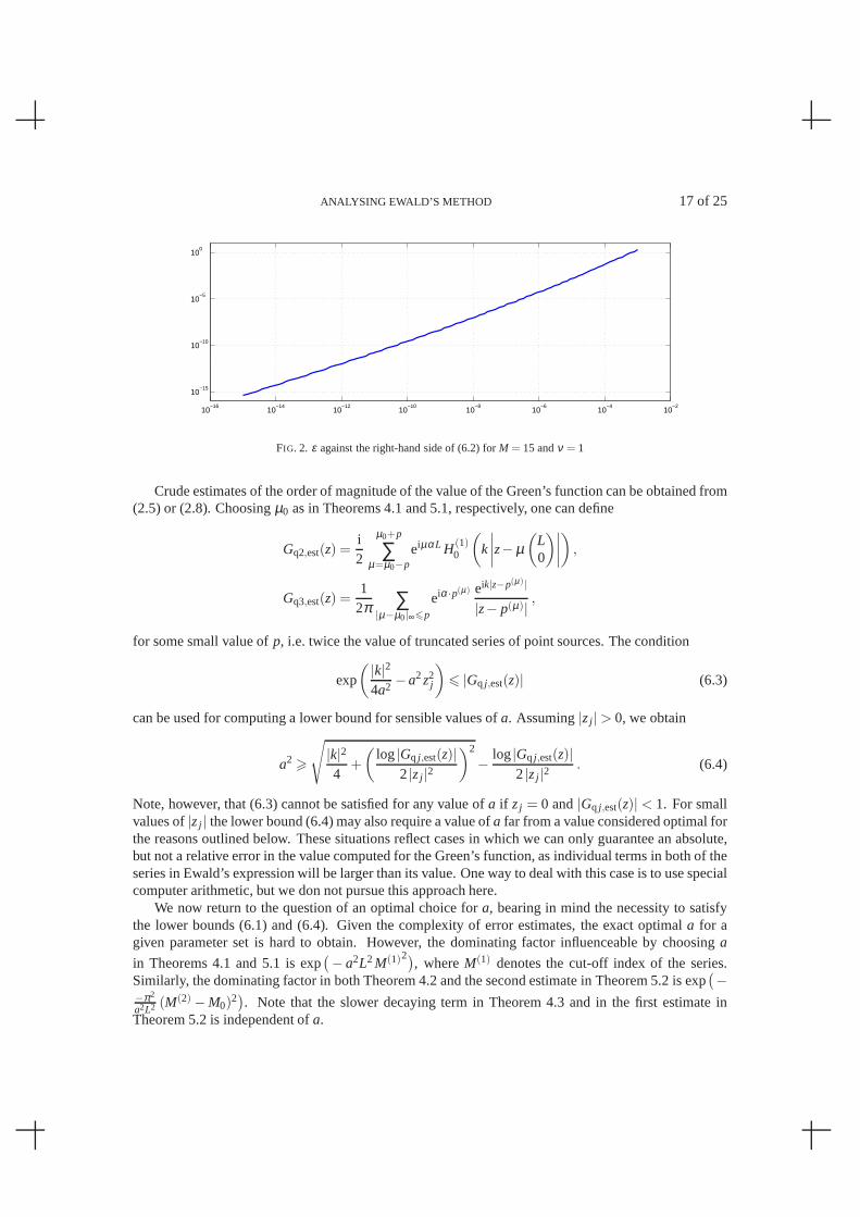
Figure 2 shows a plot ofε against the right-hand side of (6.2), demonstrating a good correspondence.

A second issue in choosinga is that care has to be taken to avoid instability and cancellation effects.The bounds on the terms in the series derived in Sections 3–5 all contain a factor exp

(

|k|2/(4a2)−a2z2j

)

,j = 2 or j = 3. The control parametera has to be chosen so that this expression is of the same order ofmagnitude as the expected value of the Green’s function to avoid cancellation effects.


10−16

10−14

10−12

10−10

10−8

10−6

10−4

10−2

10−15

10−10

10−5

100

FIG. 2. ε against the right-hand side of (6.2) forM = 15 andν = 1

Crude estimates of the order of magnitude of the value of the Green’s function can be obtained from(2.5) or (2.8). Choosingµ0 as in Theorems 4.1 and 5.1, respectively, one can define

Gq2,est(z) =i2

µ0+p

∑µ=µ0−p

eiµαL H(1)0

(

k

∣

∣

∣

∣

z− µ(

L0

)∣

∣

∣

∣

)

,

Gq3,est(z) =1

2π ∑|µ−µ0|∞6p

eiα ·p(µ) eik|z−p(µ)|

|z− p(µ)| ,

for some small value ofp, i.e. twice the value of truncated series of point sources. The condition

exp

( |k|24a2 −a2z2

j

)

6 |Gq j ,est(z)| (6.3)

can be used for computing a lower bound for sensible values ofa. Assuming|zj | > 0, we obtain

a2 >

√

|k|24

+

(

log|Gq j ,est(z)|2|zj |2

)2

− log|Gq j ,est(z)|2|zj |2

. (6.4)

Note, however, that (6.3) cannot be satisfied for any value ofa if zj = 0 and|Gq j ,est(z)| < 1. For smallvalues of|zj | the lower bound (6.4) may also require a value ofa far from a value considered optimal forthe reasons outlined below. These situations reflect cases in which we can only guarantee an absolute,but not a relative error in the value computed for the Green’sfunction, as individual terms in both of theseries in Ewald’s expression will be larger than its value. One way to deal with this case is to use specialcomputer arithmetic, but we don not pursue this approach here.

We now return to the question of an optimal choice fora, bearing in mind the necessity to satisfythe lower bounds (6.1) and (6.4). Given the complexity of error estimates, the exact optimala for agiven parameter set is hard to obtain. However, the dominating factor influenceable by choosinga

in Theorems 4.1 and 5.1 is exp(

− a2L2M(1)2), whereM(1) denotes the cut-off index of the series.

Similarly, the dominating factor in both Theorem 4.2 and thesecond estimate in Theorem 5.2 is exp(

−−π2

a2L2 (M(2) −M0)2)

. Note that the slower decaying term in Theorem 4.3 and in the first estimate inTheorem 5.2 is independent ofa.


0.2 0.4 0.6 0.8 1 1.2 1.4 1.610

−14

10−6

102

0.2 0.4 0.6 0.8 1 1.2 1.4 1.6

10−5

10−3

10−1

(a)z2 = 0.5

0.2 0.4 0.6 0.8 1 1.2 1.4 1.610

−14

10−6

102

0.2 0.4 0.6 0.8 1 1.2 1.4 1.6

10−5

10−3

10−1

(b) z2 = 0.125

0.2 0.4 0.6 0.8 1 1.2 1.4 1.610

−14

10−6

102

0.2 0.4 0.6 0.8 1 1.2 1.4 1.6

10−5

10−3

10−1

(c) z2 = 0

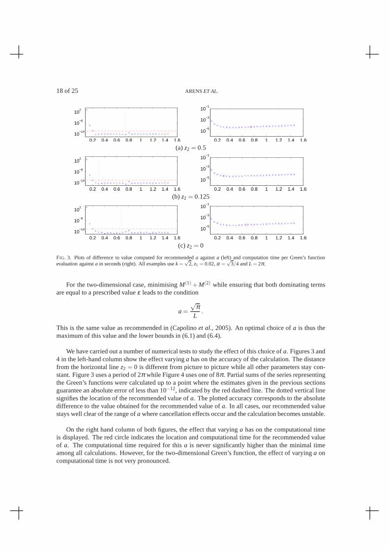
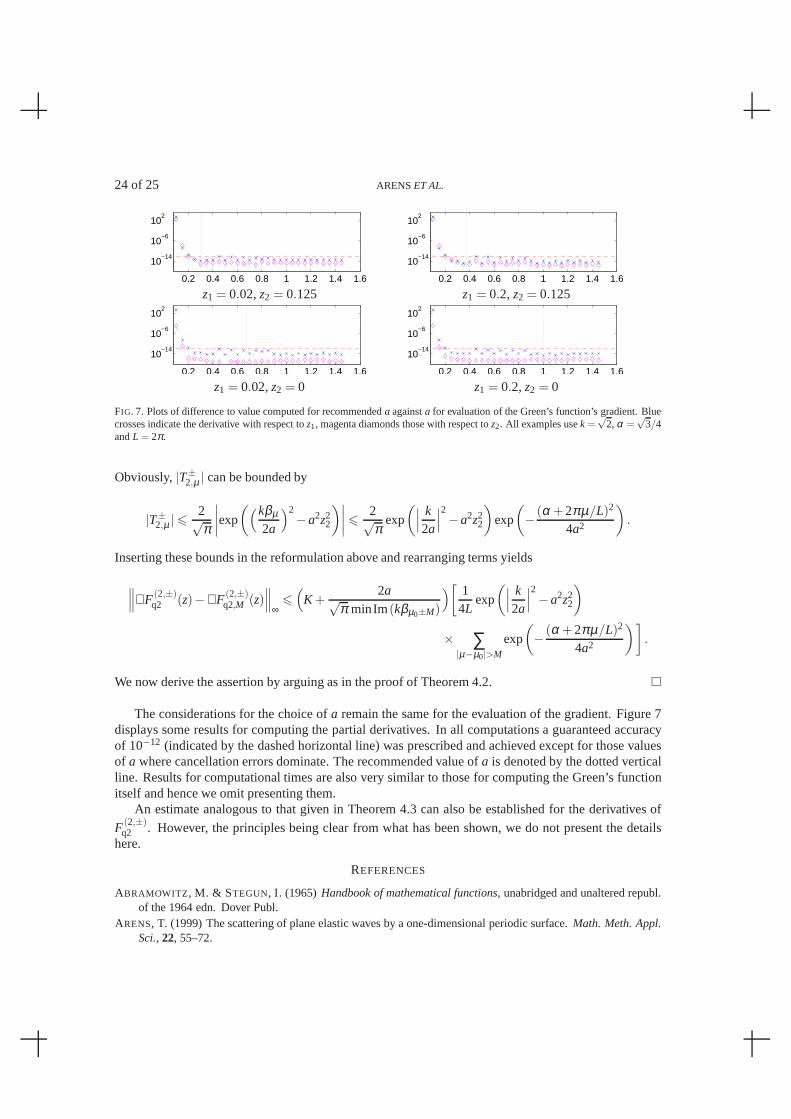
FIG. 3. Plots of difference to value computed for recommendeda againsta (left) and computation time per Green’s functionevaluation againsta in seconds (right). All examples usek =

√2, z1 = 0.02,α =

√3/4 andL = 2π.

For the two-dimensional case, minimisingM(1) + M(2) while ensuring that both dominating termsare equal to a prescribed valueε leads to the condition

a =

√π

L.

This is the same value as recommended in (Capolinoet al., 2005). An optimal choice ofa is thus themaximum of this value and the lower bounds in (6.1) and (6.4).

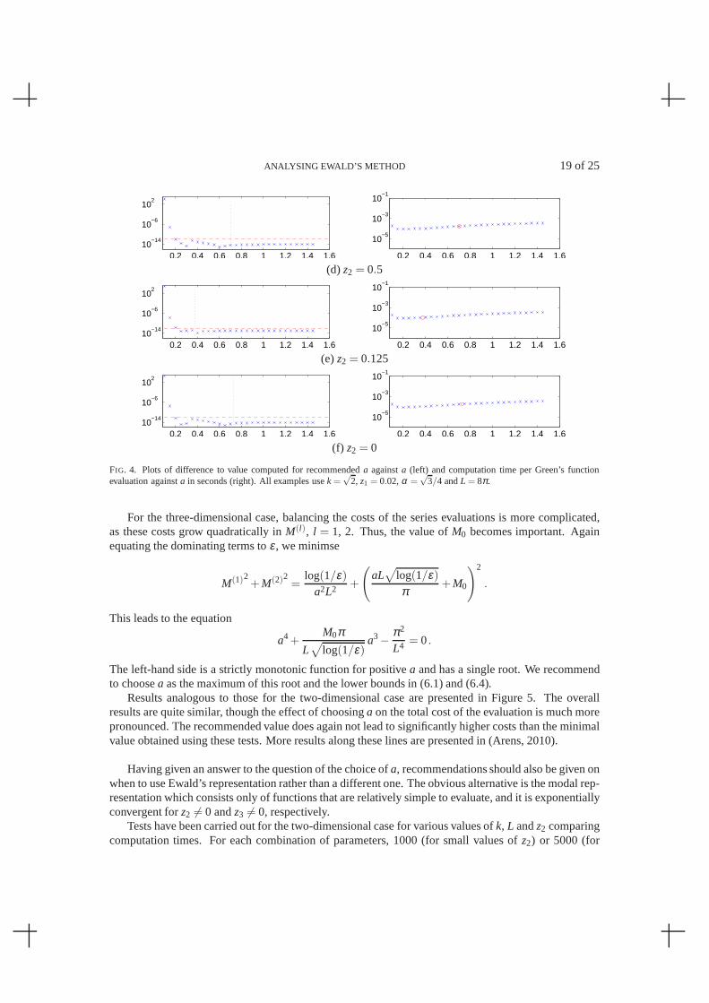
We have carried out a number of numerical tests to study the effect of this choice ofa. Figures 3 and4 in the left-hand column show the effect varyinga has on the accuracy of the calculation. The distancefrom the horizontal linez2 = 0 is different from picture to picture while all other parameters stay con-stant. Figure 3 uses a period of 2π while Figure 4 uses one of 8π . Partial sums of the series representingthe Green’s functions were calculated up to a point where theestimates given in the previous sectionsguarantee an absolute error of less than 10−12, indicated by the red dashed line. The dotted vertical linesignifies the location of the recommended value ofa. The plotted accuracy corresponds to the absolutedifference to the value obtained for the recommended value of a. In all cases, our recommended valuestays well clear of the range ofa where cancellation effects occur and the calculation becomes unstable.

On the right hand column of both figures, the effect that varying a has on the computational timeis displayed. The red circle indicates the location and computational time for the recommended valueof a. The computational time required for thisa is never significantly higher than the minimal timeamong all calculations. However, for the two-dimensional Green’s function, the effect of varyinga oncomputational time is not very pronounced.


0.2 0.4 0.6 0.8 1 1.2 1.4 1.610

−14

10−6

102

0.2 0.4 0.6 0.8 1 1.2 1.4 1.6

10−5

10−3

10−1

(d) z2 = 0.5

0.2 0.4 0.6 0.8 1 1.2 1.4 1.610

−14

10−6

102

0.2 0.4 0.6 0.8 1 1.2 1.4 1.6

10−5

10−3

10−1

(e)z2 = 0.125

0.2 0.4 0.6 0.8 1 1.2 1.4 1.610

−14

10−6

102

0.2 0.4 0.6 0.8 1 1.2 1.4 1.6

10−5

10−3

10−1

(f) z2 = 0


√2, z1 = 0.02,α =

√3/4 andL = 8π.

For the three-dimensional case, balancing the costs of the series evaluations is more complicated,as these costs grow quadratically inM(l), l = 1, 2. Thus, the value ofM0 becomes important. Againequating the dominating terms toε, we minimse

M(1)2+M(2)2

=log(1/ε)

a2L2 +

(

aL√

log(1/ε)

π+M0

)2

.

This leads to the equation

a4+M0π

L√

log(1/ε)a3− π2

L4 = 0.

The left-hand side is a strictly monotonic function for positive a and has a single root. We recommendto choosea as the maximum of this root and the lower bounds in (6.1) and (6.4).

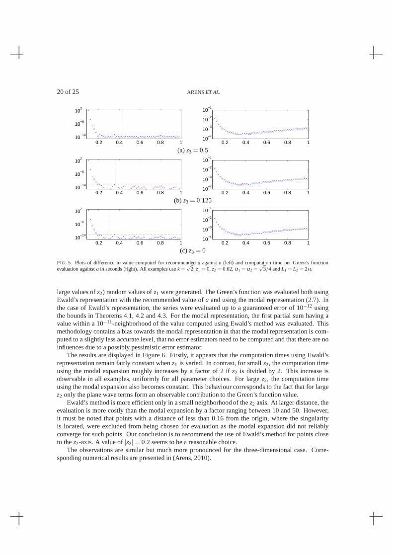
Results analogous to those for the two-dimensional case arepresented in Figure 5. The overallresults are quite similar, though the effect of choosinga on the total cost of the evaluation is much morepronounced. The recommended value does again not lead to significantly higher costs than the minimalvalue obtained using these tests. More results along these lines are presented in (Arens, 2010).

Having given an answer to the question of the choice ofa, recommendations should also be given onwhen to use Ewald’s representation rather than a different one. The obvious alternative is the modal rep-resentation which consists only of functions that are relatively simple to evaluate, and it is exponentiallyconvergent forz2 6= 0 andz3 6= 0, respectively.

Tests have been carried out for the two-dimensional case forvarious values ofk, L andz2 comparingcomputation times. For each combination of parameters, 1000 (for small values ofz2) or 5000 (for


0.2 0.4 0.6 0.8 110

−14

10−6

102

0.2 0.4 0.6 0.8 110

−4

10−3

10−2

10−1

(a)z3 = 0.5

0.2 0.4 0.6 0.8 110

−14

10−6

102

0.2 0.4 0.6 0.8 110

−4

10−3

10−2

10−1

(b) z3 = 0.125

0.2 0.4 0.6 0.8 110

−14

10−6

102

0.2 0.4 0.6 0.8 110

−4

10−3

10−2

10−1

(c) z3 = 0


√2, z1 = 0, z2 = 0.02, α1 = α2 =

√3/4 andL1 = L2 = 2π.

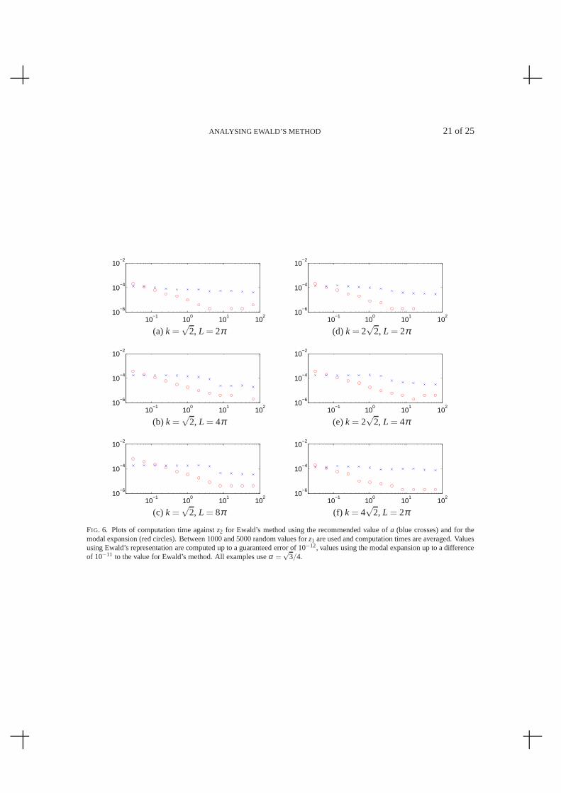
large values ofz2) random values ofz1 were generated. The Green’s function was evaluated both usingEwald’s representation with the recommended value ofa and using the modal representation (2.7). Inthe case of Ewald’s representation, the series were evaluated up to a guaranteed error of 10−12 usingthe bounds in Theorems 4.1, 4.2 and 4.3. For the modal representation, the first partial sum having avalue within a 10−11-neighborhood of the value computed using Ewald’s method was evaluated. Thismethodology contains a bias towards the modal representation in that the modal representation is com-puted to a slightly less accurate level, that no error estimators need to be computed and that there are noinfluences due to a possibly pessimistic error estimator.

The results are displayed in Figure 6. Firstly, it appears that the computation times using Ewald’srepresentation remain fairly constant whenz1 is varied. In contrast, for smallz2, the computation timeusing the modal expansion roughly increases by a factor of 2 if z2 is divided by 2. This increase isobservable in all examples, uniformly for all parameter choices. For largez2, the computation timeusing the modal expansion also becomes constant. This behaviour corresponds to the fact that for largez2 only the plane wave terms form an observable contribution tothe Green’s function value.

Ewald’s method is more efficient only in a small neighborhoodof thez2 axis. At larger distance, theevaluation is more costly than the modal expansion by a factor ranging between 10 and 50. However,it must be noted that points with a distance of less than 0.16 from the origin, where the singularityis located, were excluded from being chosen for evaluation as the modal expansion did not reliablyconverge for such points. Our conclusion is to recommend theuse of Ewald’s method for points closeto thez2-axis. A value of|z2| = 0.2 seems to be a reasonable choice.

The observations are similar but much more pronounced for the three-dimensional case. Corre-sponding numerical results are presented in (Arens, 2010).


10−1

100

101

102

10−6

10−4

10−2

10−1

100

101

102

10−6

10−4

10−2

(a)k =√

2, L = 2π (d) k = 2√

2, L = 2π

10−1

100

101

102

10−6

10−4

10−2

10−1

100

101

102

10−6

10−4

10−2

(b) k =√

2, L = 4π (e)k = 2√

2, L = 4π

10−1

100

101

102

10−6

10−4

10−2

10−1

100

101

102

10−6

10−4

10−2

(c) k =√

2, L = 8π (f) k = 4√

2, L = 2π

FIG. 6. Plots of computation time againstz2 for Ewald’s method using the recommended value ofa (blue crosses) and for themodal expansion (red circles). Between 1000 and 5000 randomvalues forz1 are used and computation times are averaged. Valuesusing Ewald’s representation are computed up to a guaranteed error of 10−12, values using the modal expansion up to a differenceof 10−11 to the value for Ewald’s method. All examples useα =

√3/4.


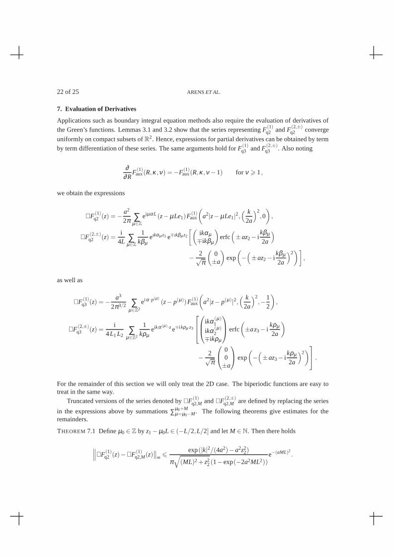
7. Evaluation of Derivatives

Applications such as boundary integral equation methods also require the evaluation of derivatives of

the Green’s functions. Lemmas 3.1 and 3.2 show that the series representingF (1)q2 andF(2,±)

q2 converge

uniformly on compact subsets ofR2. Hence, expressions for partial derivatives can be obtained by term

by term differentiation of these series. The same argumentshold forF(1)q3 andF (2,±)

q3 . Also noting

∂∂R

F (1)aux(R,κ ,ν) = −F(1)

aux(R,κ ,ν −1) for ν > 1,

we obtain the expressions

∇F (1)q2 (z) = − a2

2π ∑µ∈Z

eiµαL (z− µLe1)F (1)aux

(

a2|z− µLe1|2,( k

2a

)2,0

)

,

∇F (2,±)q2 (z) =

i4L ∑

µ∈Z

1kβµ

eıkαµ z1 e∓ıkβµ z2

[(

ikαµ∓ikβµ

)

erfc(

±az2− ikβµ

2a

)

− 2√π

(

0±a

)

exp

(

−(

±az2− ikβµ

2a

)2)]

,

as well as

∇F (1)q3 (z) = − a3

2π3/2 ∑µ∈Z2

ei α ·p(µ)(z− p(µ))F (1)

aux

(

a2|z− p(µ)|2,( k

2a

)2,−1

2

)

,

∇F (2,±)q3 (z) =

i4L1L2

∑µ∈Z2

1kρµ

eikα(µ)·ze∓i kρµ z3

ikα(µ)1

ikα(µ)2

∓ikρµ

erfc

(

±az3− ikρµ

2a

)

− 2√π

00±a

exp

(

−(

±az3− ikρµ

2a

)2)

.

For the remainder of this section we will only treat the 2D case. The biperiodic functions are easy totreat in the same way.

Truncated versions of the series denoted by∇F (1)q2,M and∇F(2,±)

q2,M are defined by replacing the series

in the expressions above by summations∑µ0+Mµ=µ0−M. The following theorems give estimates for the

remainders.

THEOREM 7.1 Defineµ0 ∈ Z by z1− µ0L ∈ (−L/2,L/2] and letM ∈ N. Then there holds

∥

∥

∥∇F(1)q2 (z)−∇F(1)

q2,M(z)∥

∥

∞ 6exp(|k|2/(4a2)−a2z2

2)

π√

(ML)2 +z22 (1−exp(−2a2ML2))

e−(aML)2.


Proof. Exactly as in the proof of Theorem 4.1, we estimate

∥

∥

∥∇F (1)q2 (z)−∇F(1)

q2,M(z)∥

∥

∥

∞6

a2exp(|k|2/(2a)2−a2z22)

2π ∑|µ−µ0|>M+1

exp(−a2(z1− µL)2)

a2√

(z1− µL)2 +z22

6exp(|k|2/(2a)2−a2z2

2)

πexp(−a2(ML)2)√

(ML)2 +z22

∞

∑µ=M+1

e−2ML2a2(µ−(M+1)) .

A geometric series argument then gives the assertion.

THEOREM 7.2 Let the assumptions of Theorem 4.3 hold and, in addition,let K be defined by

K =

maxµ∈Z

|1−1/α2µ|−1/2, if Re(k2) > Im(k2),

1, otherwise.

Then∥

∥

∥∇F (2,±)q2 (z)−∇F(2,±)

q2,M (z)∥

∥

∥

∞

6

(

K +2a√

π minIm(kβµ0±M)

) exp

(

∣

∣

k2a

∣

∣

2−a2z22−

2π2 (M−M0)

a2L2

)

2L

(

1−exp(

− 2π2 (M−M0)a2L2

)

) e−π2

a2L2 (M−M0)2.

Proof. We start with the reformulation

∥

∥

∥∇F (2,±)q2 (z)−∇F(2,±)

q2,M (z)∥

∥

∥

∞=

14L

∥

∥

∥

∥

∥

∑|µ−µ0|>M

1kβµ

eikαµ z1

[(

ikαµ∓ikβµ

)

T±1,µ +

(

0±a

)

T±2,µ

]

∥

∥

∥

∥

∥

∞

where

T±1,µ = e∓ikβµ z2 erfc

(

±az2− ikβµ

2a

)

, T±2,µ =

2√π

e∓ikβµ z2 exp

(

−(

±az2− ikβµ

2a

)2)

.

Observing that∣

∣

∣

∣

αµ

βµ

∣

∣

∣

∣

=

∣

∣

∣

∣

∣

∣

1

1− 1α2

µ

∣

∣

∣

∣

∣

∣

1/2

6 K , µ ∈ Z ,

we conclude∥

∥

∥∇F (2,±)

q2 −∇F(2,±)q2,M

∥

∥

∥

∞6

14L ∑

|µ−µ0|>M

(

K |T±1,µ |+

a|kβµ |

|T±2,µ |)

.

Similar to the argument in the proof of Theorem 4.2, we estimate |T±1,µ | by

|T±1,µ | 6 exp

(

∣

∣

∣

k2a

∣

∣

∣

2−a2z2

2

)

exp

(

− (α +2πµ/L)2

4a2

)

.


0.2 0.4 0.6 0.8 1 1.2 1.4 1.6

10−14

10−6

102

0.2 0.4 0.6 0.8 1 1.2 1.4 1.6

10−14

10−6

102

z1 = 0.02,z2 = 0.125 z1 = 0.2, z2 = 0.125

0.2 0.4 0.6 0.8 1 1.2 1.4 1.6

10−14

10−6

102

0.2 0.4 0.6 0.8 1 1.2 1.4 1.6

10−14

10−6

102

z1 = 0.02,z2 = 0 z1 = 0.2, z2 = 0

FIG. 7. Plots of difference to value computed for recommendeda againsta for evaluation of the Green’s function’s gradient. Bluecrosses indicate the derivative with respect toz1, magenta diamonds those with respect toz2. All examples usek =

√2, α =

√3/4

andL = 2π.

Obviously,|T±2,µ | can be bounded by

|T±2,µ | 6

2√π

∣

∣

∣

∣

exp

(

(kβµ

2a

)2−a2z2

2

)∣

∣

∣

∣

62√π

exp

(

∣

∣

∣

k2a

∣

∣

∣

2−a2z2

2

)

exp

(

− (α +2πµ/L)2

4a2

)

.

Inserting these bounds in the reformulation above and rearranging terms yields

∥

∥

∥∇F (2,±)q2 (z)−∇F (2,±)

q2,M (z)∥

∥

∥

∞6

(

K +2a√

π minIm(kβµ0±M)

)

[

14L

exp

(

∣

∣

∣

k2a

∣

∣

∣

2−a2z2

2

)

× ∑|µ−µ0|>M

exp

(

− (α +2πµ/L)2

4a2

)]

.

We now derive the assertion by arguing as in the proof of Theorem 4.2.

The considerations for the choice ofa remain the same for the evaluation of the gradient. Figure 7displays some results for computing the partial derivatives. In all computations a guaranteed accuracyof 10−12 (indicated by the dashed horizontal line) was prescribed and achieved except for those valuesof a where cancellation errors dominate. The recommended valueof a is denoted by the dotted verticalline. Results for computational times are also very similarto those for computing the Green’s functionitself and hence we omit presenting them.

An estimate analogous to that given in Theorem 4.3 can also beestablished for the derivatives of

F (2,±)q2 . However, the principles being clear from what has been shown, we do not present the details

here.

REFERENCES

ABRAMOWITZ , M. & STEGUN, I. (1965) Handbook of mathematical functions, unabridged and unaltered republ.of the 1964 edn. Dover Publ.

ARENS, T. (1999) The scattering of plane elastic waves by a one-dimensional periodic surface.Math. Meth. Appl.Sci., 22, 55–72.


ARENS, T. (2010) Scattering by biperiodic layered media: The integral equation approach. Habilitation Thesis,Karlsruhe Institute of Technology.

CAPOLINO, F., WILTON , D. R. & JOHNSON, W. A. (2005) Efficient computation of the 2-D Green’s function for1-D periodic structures using the Ewald method.IEEE Trans. Ant. Prop., 53, 2977–2984.

EWALD , P. P. (1921) Die Berechnung optischer und elektrostatischer Gitterpotentiale.Ann. Phys., 64, 253–287.HOPF, E. (1934)Mathematical Problems of Radiative Equilibrium. Cambridge Tracts in Mathematics and Math-

ematical Physics. Cambridge University Press.JORDAN, K. E., RICHTER, G. R. & SHENG, P. (1986) An efficient numerical evaluation of the Green’s function

for the Helmholtz operator on periodic structures.J. Comput. Phys., 63, 222–235.KAMBE , K. (1967) Theory of electron diffraction by crystals. Green’s function and integral equation.Z. Natur-

forschg., 22a, 422–431.KURKCU, H. & REITICH, F. (2009) Stable and efficient evaluation of periodized Green’s functions for the

Helmholtz equation at high frequencies.Journal of Computational Physics, 228(1), 75–95.KUSTEPELI, A. & M ARTIN , A. Q. (2000) On the Splitting Parameter in the Ewald Method.IEEE Transactions

on Microwave and Guided Wave Letters, 10(5), 168–170.L INTON, C. M. (1998) The Green’s function for the two-dimensional Helmholtz equation in periodic domains.J.

Eng. Math., 33, 377–402.MATHIS, A. W. & PETERSON, A. F. (1996) A comparison of acceleration procedures for the two-dimensional

periodic green’s function.IEEE Trans. Ant. Prop., 44, 567–571.SADOV, S. Y. (1997) Computation of quasiperiodic fundamental solution of Helmholtz equation.Advances in Dif-

ference Equations: Proceedings of the Second International Conference on Difference Equations (Veszprem,1995). CRC Press, pp. 551–558.

SANDFORT, K. (2010) The Factorization Method for inverse scatteringfrom periodic inhomogeneous media.Ph.D.thesis, Karlsruhe Institute of Technology (KIT).

Documents

Analysing Ewald’s Method for the Evaluation of Green’s ...schmitt/media/ewald-periodic.pdf · Analysing Ewald’s Method for the Evaluation of Green’s Functions for Periodic