Embed Size (px)
Citation preview

MASTER THESIS – MIKE LAMERS – MORPHOLOGY IN THE VECHT – I
Analysing the morphological consequences of the preferred design of the Overijsselse Vecht with SOBEK 3.
Mike Lamers 19-01-2017

MASTER THESIS – MIKE LAMERS – MORPHOLOGY IN THE VECHT – II
Analysing the morphological consequences of the preferred design
of the Overijsselse Vecht with SOBEK 3.
MSc Thesis Final version
Author:
Name Ing. M.J.M. Lamers
Student number s1589415
Contact [email protected]
Under supervision of:
Dr. Ir. D.C.M. Augustijn Graduation supervisor of University of Twente
Dr. J.J. Warmink Daily supervisor of University of Twente
Ir. J. van der Scheer Supervisor Water board Vechtstromen
Date 19-01-2017
University of Twente, Enschede
Faculty of Engineering Technology
Water engineering and Management (WEM)
Water board Vechtstromen, Almelo

MASTER THESIS – MIKE LAMERS – MORPHOLOGY IN THE VECHT – I
Preface
For my graduation project I was looking for a bit more technical project, in which I could link the
theoretical background of the master Water Engineering and Management (WEM) at the University
of Twente with a realistic case. About 6 months ago I started my graduation research at water board
Vechtstromen in Almelo about the morphological processes in the redeveloped Overijsselse Vecht.
During this research I clearly noticed that a realistic situation also involves realistic problems you
have to deal with. This study mainly consists of simulations of models in the software programme
SOBEK 3 which induced several modelling issues. I want to thank K.D. Berends for his help and
guidance in finding bugs and thinking about solutions during construction of the models.
This research could not be produced without the opportunity of water board Vechtstromen to
research this subject. During this process, I am greatly supported by my supervisors Ir. J. van der
Scheer (water board Vechtstromen), Dr. Ir. D.C.M. Augustijn and Dr. J.J. Warmink from the
University of Twente for who I want to express my gratitude! I also want to thank my family and
girlfriend Sandra for listening and supporting during times of modelling struggles.
Mike Lamers
Enschede, 19th of January 2017

MASTER THESIS – MIKE LAMERS – MORPHOLOGY IN THE VECHT – II

MASTER THESIS – MIKE LAMERS – MORPHOLOGY IN THE VECHT – III
Summary In 2005 the water boards Velt and Vecht (now Vechtstromen) and Groot Salland (now Drents
Overijsselse Delta) took over the management and maintenance of the Overijsselse Vecht from
Rijkswaterstaat (Ministry of Infrastructure and the Environment). Since that moment the water
boards have obligated themselves to meet the guidelines for the Vecht according to inter alia the
Water Framework Directive WFD and Natura 2000. This obligation was proposed in 2009 in the
‘Vechtvisie 2009’, which is about the redevelopment of the canalised Vecht into a living half-natural
lowland river. This includes meandering, sedimentation and erosion processes. After
implementation of several measures more dynamics will be created. Based on several different
alternatives (Wolfert et al., 2009a) and hydraulic simulations, a preferred alternative was
accomplished. Water board Vechtstromen wanted an indication of the amount of sedimentation
and erosion, where these processes would take place in the preferred situation over a period of 35
years and what the effect is on the prerequisites for safety and recreational navigability.
The main objective of this research is:
Analysing and understanding the morphological processes in the Overijsselse Vecht and quantifying
the morphological consequences for bed and water level changes for the preferred alternative by
using a SOBEK 3 model.
The SOBEK 3 models of the current situation and preferred alternative are based on existing SOBEK
2 models previously developed by water board Vechtstromen. The model schematisations are
simplified by removing small fish ladders and insignificant lateral flows. The studied reach has a
length of approximately 45 and 56 kilometres for respectively the current and preferred situation.
The morphological behaviour is investigated between Emlichheim (upstream boundary) and
Vilsteren (downstream boundary) which is divided in 5 reach segments. The main differences in
current and preferred situation are the target (water) levels of the reach segments, the amount of
meandering (increasing length), widths and depths of the Vecht. The available discharge data,
which are the boundary conditions of the model, turned out to be incorrect and incomplete and
therefore not directly usable. These discharges are corrected and used for calibration and validation
of the hydraulic and morphological SOBEK 3 models of the current situation.
The calibrated roughness values of the main channel (Chézy) and the floodplains (Strickler kn) are
used in the morphological calibration of the current situation. Based on 3 bed level observations (in
2008, 2010 and 2013) the sediment inflow at Emlichheim and the transport parameter are
calibrated using the sediment transport formulas of Engelund and Hansen (1967).
After modelling the current situation and the preferred alternative over 35 years, simulation results
show that the Vecht is a quite morphological active river, which yearly transports on average
between 1200 and 15000 m3/s, depending on the location. In the current situation and in the
preferred alternative, sediment inflow starts depositing upstream between Emlichheim and De
Haandrik. Peak discharges seem to stimulate more sediment transport in downstream direction.
Bed levels during low discharges show hardly effects of peak discharges. This is often related to the
main channel widths. In the current situation there are more locations with stronger erosion,
caused by smaller main channel widths compared to the preferred alternative. A fluctuating width
causes also fluctuating bed levels. The preferred alternative is more stable, due to wider main
channels, causing smaller sediment transport capacities.
During peak discharges, morphological behaviour is not dependent on the main channel width but
on the width of the floodplains. Decreasing floodplain widths (in flow direction) induce an increase

MASTER THESIS – MIKE LAMERS – MORPHOLOGY IN THE VECHT – IV
in flow velocity causing larger sediment transport capacities. Large fluctuations in floodplain widths
cause large variability in bed levels with often large erosion pits. When these peak discharges
decrease, the erosion pits fill up due to less fluctuating main channels.
For both the current situation as the preferred alternative, the bed level development between
Emlichheim and De Haandrik seemed to go towards a dynamic equilibrium when comparing an
additional run of 68 years with the run of 35 years. The difference in bed levels between Emlichheim
and De Haandrik are quite small and sediment deposition is propagating in downstream direction.
It is expected that when no maintenance is applied, all bed levels of the Vecht will be increased
with approximately 1 till 2 meters after a couple of hundred years.
The prerequisites for safety and recreational navigation are checked. The minimal water depth of
0.5 meter is met at all locations in the area of water board Vechtstromen. After 35 years of bed
level development, without dredging activities, bed levels increase between Emlichheim and
approximately 18 km downstream (of which 10 km belongs to Vechtstromen), resulting in an
exceedance of the maximum water levels up to 30 cm. The exceedance already starts after one year
and increases over time. To keep the maximum water level at the normative level it is required to
dredge on a regular basis, which has been done almost each year (Vogelsang, 2016). This prevents
further deposition of sediment more downstream. The dredged materials can be put back into the
river more downstream in erosion pits or other locations. This sediment will again be transported
downstream without causing problems.
The two studied measures, flood channels and floodplain forest, induce only effect during higher
discharges. During peak discharges, the 15 flood channels cause differences in bed level at the
bifurcation and confluence of the flood channel, which will disappear after the peak discharge. The
floodplain forests have hardly effect on the bed levels. Both measures have no effect on the
maximum water levels or water depths, caused by changing bed levels, and therefore need no
additional maintenance.

MASTER THESIS – MIKE LAMERS – MORPHOLOGY IN THE VECHT – V
Table of contents Preface ................................................................................................................................................ 1
Summary ............................................................................................................................................ 3
1. Introduction ................................................................................................................................ 1
1.1. History and plans of the Vecht ........................................................................................... 1
1.2. Problem definition .............................................................................................................. 2
1.3. Research objective ............................................................................................................. 2
1.4. Research questions............................................................................................................. 2
1.5. Methodology and report outline ........................................................................................ 3
2. Set-up and calibration of the hydraulic SOBEK 3 model ............................................................ 5
2.1. Outline of study area .......................................................................................................... 5
2.2. SOBEK 3 schematisation ..................................................................................................... 5
2.3. Boundary conditions .......................................................................................................... 8
2.4. Calibration and validation of roughness coefficients ....................................................... 10
3. Set-up and calibration of the morphological SOBEK 3 model .................................................. 15
3.1. Model set-up .................................................................................................................... 15
3.2. Morphological model settings in SOBEK 3 ....................................................................... 16
3.3. Method of calibration sediment inflow and transport parameter .................................. 18
3.4. Results calibration ............................................................................................................ 19
3.5. Validation of total reach ................................................................................................... 22
4. Morphology of the new Vecht ................................................................................................. 23
4.1. Model set-up of preferred alternative ............................................................................. 23
4.2. Methodology .................................................................................................................... 24
4.3. Short-term results – morphological consequences of different discharges .................... 25
4.4. Intermediate-term – Bed level development over 35 years ............................................ 29
4.5. Long-term behaviour – Towards a dynamic equilibrium bed level .................................. 32
4.6. Check of prerequisites ...................................................................................................... 33
5. Influence of measures .............................................................................................................. 36
5.1. Methodology .................................................................................................................... 36
5.2. Results .............................................................................................................................. 36
6. Discussion ................................................................................................................................. 39
7. Conclusion and recommendations ........................................................................................... 40
7.1. Conclusion ........................................................................................................................ 40
7.2. Recommendations............................................................................................................ 41
References ........................................................................................................................................ 43
Appendix 1 - Determination of corrected 35-years discharge series ............................................... 44
Appendix 2 – Calibration results main channel ................................................................................ 49

MASTER THESIS – MIKE LAMERS – MORPHOLOGY IN THE VECHT – VI
Appendix 3 – Calibration of the floodplain ...................................................................................... 50
Appendix 4 – Validation results ........................................................................................................ 51
Appendix 5 – Calculations for check suitability of Engelund and Hansen ........................................ 52
Appendix 6 – Measures of the preferred alternative ....................................................................... 53
Appendix 7 – Different locations for each type ............................................................................... 54
Appendix 8 – T=200 discharge waves .............................................................................................. 55
Appendix 9 – Analysis of behaviour in front of weir Hardenberg .................................................... 56
Appendix 10 – Total sediment transport and accretion on 6 moments .......................................... 57

MASTER THESIS – MIKE LAMERS – MORPHOLOGY IN THE VECHT – 1
1. Introduction This chapter contains the historical evolvements of the Vecht and the problem definition. Based on
the problem definition, a research objective is formulated followed by subsequent research
questions. This thesis often refers to the current situation (2016) and preferred alternative. The
current situation is the shape of the river at this moment and the preferred alternative is the
redeveloped situation of the river after implementing the measures of the preferred alternative.
1.1. History and plans of the Vecht In former times, the Vecht was a strong meandering river with (mainly in Germany) a large drop in
altitude. At the moment, the Vecht has a length of 167 kilometres and a total drop of 105 meters
of which 10 meters in the Netherlands. The river originates from Rosendahl, a community in
Noordrijn-Westfalen (Germany), crosses the border at Emlichheim and ends in the river Zwarte
Water at Zwolle (Netherlands), see Figure 1. The Vecht is a rainfed river, which gives a strong varying
discharges over time. The large drop in elevation and a changing function of the area near the Vecht
initiated several interventions at certain moments, which made the Vecht a controlled and
canalised river. This includes cutting off 69 meanders and therefore reducing the length with 30
kilometres and increasing the slope which gave increased vertical erosion. Several weirs were
placed in the Vecht to prevent this process. At the moment these weirs make it possible to control
the dynamics of the river. The current level regulation of the weirs is designed to counteract bed
erosion, but also to optimise the agricultural conditions, located on the floodplains. These
interventions also have impact on the vegetation, fish migration and morphology within the Vecht
(Wolfert et al.,2009a).
Since 1997, a preliminary policy or plan
about the Vecht was proposed as the
‘Vechtvisie 1997’. However, in 2005 the
water boards Velt and Vecht (now
Vechtstromen) and Groot Salland (now
Drents Overijsselse Delta) took over the
management and maintenance of the
river from Rijkswaterstaat (Ministry of
infrastructure and the environment). At
that moment the water boards have
also obliged themselves to actualise the
Dutch part of the Vechtvisie 1997
according to, inter alia, the Water
Framework Directive WFD and Natura
2000. The province Overijssel
stimulates and coordinates actively in
the context of the program ‘Room for
the Vecht’, to ensure water safety,
economical and socio-economic
development of the Vecht valley, but
also to realise ecological objectives
(Province Overijssel, 2009). This
obligation was established in 2009 in
the ‘Vechtvisie 2009’ (DHV & NWP,
2009).
Figure 1 - Total length of the Vecht from source (Rosendahl) to mouth (Zwarte Water near Zwolle)

MASTER THESIS – MIKE LAMERS – MORPHOLOGY IN THE VECHT – 2
This vision is about the redevelopment of the canalised Vecht into a living half-natural lowland river,
which will have meandering, sedimentation and erosion processes. After redevelopment, (old)
isolated meanders will be connected again, inundation areas are created or floodplains lowered.
The main channel of the Vecht itself will be shoaled and widened. More dynamics are created by
adapting more natural water levels, creation of pools in the floodplains, creation of bypasses at
weirs, removal of bank revetment (where possible) and creation of environmentally-friendly banks,
buffer strips and afforestation. From several different alternatives (Wolfert et al., 2009a), a
preferred alternative was composed (Toorn, 2016) which consists of some of the above mentioned
measures.
1.2. Problem definition The preferred alternative has been simulated in a SOBEK 2 Rural model of water board
Vechtstromen and evaluated according the prerequisites (Toorn, 2016). This simulation is based on
hydraulic calculations without taking morphology into account. At the moment, the bed of the
Vecht seems quite stable. However, the Vecht in the preferred condition has a different shape (i.e.
length, width, depth and slope) and water levels are regulated differently which gives different
hydraulic conditions. This change in hydraulic behaviour could influence morphological processes
in the Vecht as there is continuous interaction between the hydraulic and morphology
characteristics (Ribberink, 2011). Despite the importance of morphological processes, there is
within Vechtstromen a lack of knowledge about what the morphological processes in the Vecht are
and how these change for the preferred alternative. Water board Vechtstromen wants to get an
indication of the amount of sedimentation and erosion, where these processes are likely to take
place for the preferred alternative over 35 years from 2015 and what the effects are on the safety
and navigability. Also the effects of two major measurements, which are flood channels and
floodplain forests in the preferred alternative have been studied.
1.3. Research objective The main objective of this research is:
Analysing and understanding the morphological processes in the Overijsselse Vecht and quantifying
the morphological consequences for bed and water level changes for the preferred alternative by
using a SOBEK 3 model.
This objective is achieved by setting-up a morphological SOBEK 3 model and simulating 35 years of
morphological processes. These processes can induce different water levels and depths in the
preferred alternative which will be translated to certain maintenance recommendations.
1.4. Research questions The main research question of this research is:
Where and in what order of magnitude will morphological processes as sedimentation and erosion
change due to implementing the preferred alternative of the Vecht and what consequences does it
have on maintenance?
The research question is split up into two parts. The first part is developing a SOBEK 3 model, with
the following questions and sub questions:
Question 1: In what way can the hydraulic SOBEK 2 Rural model be migrated to the hydraulic
SOBEK 3 model for the current situation?
o Sub question 1.1: What is the study area and how can it be schematised in SOBEK 3?

MASTER THESIS – MIKE LAMERS – MORPHOLOGY IN THE VECHT – 3
o Sub question 1.2: What boundary conditions (BC) does the model need and how are
these determined?
o Sub question 1.3: What are the calibrated roughness values for the main channel and
floodplain for the current situation?
Question 2: What are the most appropriate morphological parameter values for the SOBEK 3
model of the current situation?
o Sub question 2.1: What is the best sediment transport formula to be used for
morphological calculations?
o Sub question 2.2: What are the most optimal values for the parameters sediment inflow
at Emlichheim and transport parameter α of the transport formula?
o Sub question 2.3: How well does the model describe the morphological behaviour?
Part 2 of the research is the application of the morphological SOBEK 3 model of the preferred
alternative, to be able to answer the following questions:
Question 3: What is the morphological behaviour during 35 years of discharge events in the
current situation and preferred alternative and what consequences does this behaviour have?
o Sub question 3.1: What are the morphological consequences of different discharge
events in the preferred alternative?
o Sub question 3.2 What is the morphological behaviour in the current and preferred
situation over 35 years (2015-2050) of modelling and does it reach an equilibrium level?
o Sub question 3.3: Does the preferred alternative meet the prerequisites until 2050?
Question 4: What are the effects of the floodplain forest and flood channels in the preferred
alternative on the morphological processes and what recommendations can be given based on
that?
1.5. Methodology and report outline This thesis describes the development of a SOBEK 3 model of the Vecht capable of simulating the
morphological processes. Chapter 2 starts with framing the study area which continues in the
development of the hydraulic SOBEK 3 model of the current situation. The roughness coefficients
are calibrated and validated in this chapter. Chapter 3 describes the choice of sediment transport
formula, required model adaptations and the calibration of the sediment inflow at the upstream
boundary and the transport parameter.
Chapter 4 analyses the morphological
behaviour of the current and preferred
situation. It contains the effect of discharge
events in the long and short term and
evaluates the prerequisites. Chapter 5
describes the sensitivity of the applied
measures in the preferred alternative on
the morphological processes. The
discussion about assumptions and results
is included in chapter 6. Chapter 7 contains
the conclusion, answering the questions of
this research and the recommendations
according morphological modelling,
science and for practice. Figure 2 - Report outline

MASTER THESIS – MIKE LAMERS – MORPHOLOGY IN THE VECHT – 4

MASTER THESIS – MIKE LAMERS – MORPHOLOGY IN THE VECHT – 5
2. Set-up and calibration of the hydraulic SOBEK 3 model
This chapter describes the study area and set-up of the hydraulic SOBEK 3 model of the current
Vecht. Morphological predictions are based on hydraulic characteristics (i.e. flow velocities)
(Ribberink, 2011). The hydraulic characteristics are reproduced by schematising the model as
accurate as needed and calibration of the main channel and floodplain roughness. The next sections
describe the components of the SOBEK 3 schematisation and the calibration of the hydraulic model.
2.1. Outline of study area The study area of this research is the Vecht reach from Emlichheim (Germany) until the weir at
Vilsteren (Netherlands), consisting of a total length of 44.5 km in the current situation. 7.7 km is
located in Germany (Emlichheim – Laar) and 3.2 km is located in water board Drents Overijsselse
Delta (wDOD, from Vilsteren – Varsen (Ommen)). Between these parts, the Vecht is managed by
water board Vechtstromen (Laar – Varsen (Ommen)). The choice of this study area is based on the
following aspects:
This reach corresponds with the existing SOBEK 2 models of the current situation and
preferred alternative modelled by water board Vechtstromen;
Between Emlichheim and the border, no lateral flows enter or sediment traps are present
which makes it the most useful location to calibrate the inflow of sediment and sediment
transport, based on performed bottom level measurements in 2008 and 2013.
Weir Vilsteren is located outside water board Vechtstromen but has a large influence on
the water levels inside water board Vechtstromen. This boundary can function
conveniently as a Q(H) boundary in the SOBEK 3 model.
Mentioned reaches, borders, weirs in the Vecht and lateral flows merging with the Vecht are shown
in Figure 3.
Figure 3 - Study area for this research
2.2. SOBEK 3 schematisation SOBEK 3 is a one dimensional modelling package for modelling open channel flow and rainfall-
runoff processes. Steady and non-steady flow, salt intrusion, sediment transport, morphology and

MASTER THESIS – MIKE LAMERS – MORPHOLOGY IN THE VECHT – 6
water quality can be simulated. SOBEK 3 is developed by Deltares as a successor to both SOBEK-RE
(River Estuary) and SOBEK-RU (Rural/Urban, also known as SOBEK 2). The choice for using SOBEK 3
is due to the improved computational capacities for morphological calculations compared to SOBEK
2. The schematisation of the SOBEK 3 model is based on the existing SOBEK 2 RU model of water
board Vechtstromen and consists of a network, cross-sections with roughness coefficients and
structures (e.g. bridges, culverts, and weirs), described below.
2.2.1. Network The network of the SOBEK 3 model is simplified compared to the original SOBEK 2 model. Small fish
ladders or bypasses around weirs of the main Vecht and the bypasses at the Vechtpark in
Hardenberg are ignored due to large required computation time and small to no effects on the
sediment transport or hydraulics of the main channel. The amount of discharge stays equal due to
the regulation of a constant water level. During low discharges, little to none sediment transport
occurs and during large discharges the weirs in the main channel are lowered and water flows on
top of the floodplains in which these bypasses and fish ladders are located and therefore have no
effect on sediment transport. Field exploration also shown that almost no sedimentation took place
at the fish ladders due to the constant presence of high flow velocities. The larger bypasses at
Mariënberg and Junne are taken into account. The secondary channels Loozensche Linie and
Uilenkamp are also included in the SOBEK 3 models of the current and preferred situation. In this
research the lateral flows Regge (1), Ommerkanaal (2), Junne-Ommenbrug (3), Mariënberg-
Vechtkanaal (4), Radewijkerbeek (5), Afwateringskanaal (6) and the Coevordenkanaal (7) (visible in
Figure 3) are taken into account. This means that each reach segment between two weirs has a
lateral inflow. The contribution in discharge of these laterals is shown in Table 2.
2.2.2. Cross-sections The SOBEK 2 models (current and preferred situation) contains symmetric YZ cross-sections of the
Vecht and asymmetric YZ cross-sections of the secondary channels and lateral flows. One of the
restrictions for morphological calculations in SOBEK 3 is that ZW cross-sections should be used.
These cross-sections have for a certain water level Z a certain width W. SOBEK 3 calculates with the
hydraulic radius which should be equal for the YZ and ZW profiles. It is easy to transform the
symmetric YZ cross-sections into ZW cross-sections. The asymmetric cross-sections on the other
hand are more difficult to transform. This is done by interpolating between the YZ points of the
cross-section and determine for each Y the width W of the cross-section. In this case the same wet
area A and wet perimeter P are obtained which gives the same hydraulic radius R (R=A/P). For the
preferred alternative the same method is applied to determine the new ZW cross-sections for the
SOBEK 3 model.
Figure 4 - Example transformation asymmetric YZ cross-section to symmetric ZW cross-section, with equal R and A.

MASTER THESIS – MIKE LAMERS – MORPHOLOGY IN THE VECHT – 7
The bed levels of the SOBEK 2 cross-sections are checked with the bed level measurements of June
2008. This is done for the bed levels of the cross-sections in the Vecht and its secondary channels
Loozensche Linie and Uilenkamp as for those channels measurements are available. For hydraulic
calibration this is less important, but for morphological calibration this gives a better starting
position. The monitoring results show asymmetric cross-sections in bends and more symmetric
cross-sections in straight branches. The bed levels are taken in the middle of the river to obtain an
average in bed level. SOBEK 3 is one-dimensional and also computes bed level changes over the
complete width of the channel. It shown that there were significant differences between the bed
levels of the available cross-sections and observed bed levels. Due to the large variation of width of
the Vecht valley (between 100 and 3200 meter), there are approximately 360 different cross-
sections in the model. Within these cross-sections also different flow and storage widths are applied
due to the variance in vegetation. The flow and storage widths of the SOBEK 2 model are copied.
2.2.3. Roughness coefficients In the SOBEK 2 models the symmetric YZ cross-sections are divided into the main channel with a
Chézy roughness C [m1/2/s] and the floodplains with a Strickler roughness kn [-]. The main Chézy
values for the main channel are 35 m1/2/s (most of the bed width) and 4.99 m1/2/s (banks of main
channel). The Strickler roughness at the floodplains depends on the type of vegetation and location
at the floodplain. The main values for the Strickler roughness coefficient kn are 0.20, 0.21 and 0.31,
resulting in Chezy values C according to Eq. ( 1 ) with R as the hydraulic radius [m].
Chézy coefficient C [m/s1/2] 𝐶 = 25 (𝑅
𝑘𝑛)
16
Eq. ( 1 )
The roughness coefficients for the complete widths of the secondary channels and laterals in SOBEK
2 are determined with the Bos & Bijkerk parameter 𝛾 [1/s]. This parameter indicates the
(maintenance) condition of the channel and is set on 33.8 1/s. This parameter 𝛾 and the water
depth d [m] are used in Eq. ( 2 ) to determine the Manning coefficient n [s/m1/3] (Deltares, 2013).
Manning roughness coefficient [s/m1/3] 𝑛 = 𝛾𝑑13 Eq. ( 2 )
This can be rewritten as a Chézy coefficient as a function of the hydraulic radius R [m]:
Chézy coefficient [m/s1/2]: 𝐶 = 𝑛𝑅16 Eq. ( 3 )
In the SOBEK 3 models of the current and preferred situation the roughness of the main channel
and flood channels are set to a Chézy roughness and the floodplains are set to a Strickler kn
roughness. Secondary channels consist of the Bos & Bijkerk roughness coefficient of 33.8 [1/s] as in
the SOBEK 2 models. Only the main channel is morphological active in SOBEK 3 of which the
sediment transport is determined with the average flow velocity of the main channel and the
floodplains.
2.2.4. Structures and their regulation Within the schematisation of the SOBEK 3 models for the current situation, constructions as
bridges, culverts and simple weirs are taken into account. The characteristics (type, size, levels and
roughness) of these structures are exactly copied from the SOBEK 2 model. SOBEK 2 and 3 are one-
dimensional, which makes it impossible for water to flow over the floodplain passing the weir
sideways during high water (like in reality). This requires the construction of a second weir in the
schematisation. The width of the second weir corresponds to the width of the floodplain (at the
weir). The fixed height of this weir is the average height of the floodplain at the location of that
weir. In SOBEK 3 these two weirs are implemented as composite structures. The levels of the weirs

MASTER THESIS – MIKE LAMERS – MORPHOLOGY IN THE VECHT – 8
in the floodplain are based on the levels of the Rijkswaterstaat SOBEK 3 model of the Vecht (Van
der Mheen, 2015). This model is not used as it is less detailed compared to the SOBEK 2 model of
water board Vechtstromen. The characteristics of the four weirs are given in Table 1 and the
locations are shown in Figure 3.
Table 1 - Characteristics of weirs in the Vecht
Units De Haandrik Hardenberg Mariënberg Junne
Weir in main channel Summer level m +NAP 9.15 7.10 5.60 4.50 Winter level m +NAP 9.10 6.80 5.20 4.15 Width m 21.00 27.00 27.00 27.00 Minimum level m +NAP 6.96 5.18 3.88 2.67 Maximum level m +NAP 9.17 7.09 5.97 4.81 Weir in floodplain Fixed weir level m +NAP 9.58 7.63 6.30 5.50 Width weir m 21.00 45.00 27.00 30.00
The weirs in the main channel of the Vecht are regulated with a PID controller, implemented in the
real time control (RTC) module. A proportional–integral–derivative controller (PID controller) is a
control-loop feedback mechanism, which continuously calculates an error value as the difference
between a desired setpoint (target level) and a measured process variable (simulated water level
at observation point) and applies a correction based on proportional P, integral I, and/or derivative
D terms (Deltares, 2013b). In these models only the P term is used and set on 1. During high
discharges, the weir can drop with a speed of 0.001 m/s until its minimum level.
Figure 5 - Schematisation of the network in SOBEK 3
2.3. Boundary conditions
2.3.1. Type of conditions The inflow at Emlichheim and lateral inflows are boundaries of the system which are based on
discharge series Q(t). The downstream boundary condition at Vilsteren is based on water levels
related to a certain discharge, Q(H). The simplified system is shown in by Figure 5. The input for the
time dependent discharge boundaries are based on observations of measurement stations. These
measurement stations determine discharges with a Q(H) relation or an acoustic device which

MASTER THESIS – MIKE LAMERS – MORPHOLOGY IN THE VECHT – 9
measures flow velocities and water levels. The Q(H) relation is indicated by ST and the acoustic
device by DM in Table 2 and Figure 5. Next section describes the computation of the discharge
series.
2.3.2. Required discharge series To compute all simulations, the following different discharge series of Emlichheim and all laterals
are required to predict the futuristic morphological behaviour.
Hydraulic calibration of roughness: January 2008 – March 2008
Hydraulic validation of roughness: January 2009 – April 2009
Morphological calibration: June 2008 – May 2013
Futuristic morphological behaviour: 2015 – 2050
Table 2 shows two problems according the availability of discharge series. First, the series are too
small to compute a 35-years series. The second are the inconsistent results of the discharges for
equal return periods. This is not only for the return periods, but also for daily discharge
measurements (see Appendix 1). This needs the following aspects:
Construction of a 35-years discharge series
Correction of this series to make a closed water balance
The construction of the 35-years discharge series is based on the 35-years water level series of
1980-2015 at Emlichheim and the corresponding Q(H) relation (for more details, see Appendix 1).
The correction of this discharge series is performed by making use of the work of Jeroen van der
Scheer, hydrologist of water board Vechtstromen, who investigated the data in 2015 and
determined corrected discharges for 8 different return periods at each measurement station in the
Vecht (Van der Scheer, 2015). Each moment of the 35-years observed discharge series has a certain
exceedance frequency (based on the corresponding discharge). Each return period of Table 2 has a
certain exceedance frequency. When interpolating the discharges of these return periods, the
discharges corresponding to the exceedance frequencies of the 35-years series can be determined
(see Appendix 1). The exceedance frequencies are linked to a date, which makes it possible to sort
it again. This is done for each station.
The new series are used for the calibration of the hydraulic and morphological model of the current
situation but also for the prediction of morphological activities in the preferred alternative. The
reasons and more detailed methods are explained in Appendix 1.
Table 2 - Observed (Obs.) and Corrected (Corr.) discharges [m3/s] at the measurement stations for different return periods with 1/2 Q is 20 days a year, 1/4 Q is 80 days a year and 1/100 Q is 347 days a year.
Type: Station ST Lateral Station DM Station ST Lateral Station ST Lateral
Return period
Emlichheim Emlichheim-Haandrik
De Haandrik De Haandrik Afwaterings-kanaal
Hardenberg Radewijker-beek Obs. Corr. Obs. Corr. Obs. Corr. Obs. Corr.
T=200 247 2 249 249 66 315 21
T=100 236 2 238 238 62 300 20
T=25 214 1 215 215 51 266 16
T=10 199 1 200 168 200 48 150 248 16
T=1 112 115 1 116 116 89 116 34 144 150 10
1/2Q 53 55 1 62 56 58 56 16 83 74 5
1/4Q 22 23 0 28 23 24 23 7 33 30 2
1/100Q 4.7 0.5 0 0.5 0.5 0.5 0.5 0.1 0.5 0.6 0

MASTER THESIS – MIKE LAMERS – MORPHOLOGY IN THE VECHT – 10
Type: Station ST Lateral Station ST Lateral Station DM Lateral Station ST
Return period
Mariënberg Mariënberg-Vechtkanaal
Junne Junne- Ommenbrug
Ommenbrug Ommerkanaal and Regge
Vilsteren
Obs. Corr. Obs. Corr. Obs. Corr. Corr.
T=200 336 11 347 8 355 145 500
T=100 320 10 330 8 338 140 478
T=25 284 9 293 7 300 120 420
T=10 186 264 8 532 272 7 194 279 105 384
T=1 156 160 5 287 165 4 167 169 70 239
1/2Q 72 79 3 81 82 2 84 84 37 121
1/4Q 31 32 2 32 34 1 35 35 18 53
1/100Q 0.2 0.6 0 0.2 0.6 0.1 1.7 0.7 1.7 2.4
2.4. Calibration and validation of roughness coefficients The goal is to find a roughness for which the simulated water levels are as close as possible to the
observed water levels by using the corrected discharge. A validation is done to indicate the
performance of the model for a different time period.
2.4.1. Calibration method The calibration is based on water levels and discharges from June 2008 as the SOBEK model is set-
up with measured bed levels available from that year. This gives the best representation of reality.
The total reach is divided into 5 reach segments (between two weirs) as these reach segments are
independent of each other during lower discharges due to sufficiently large head differences at the
weirs. Table 3 shows the measurement stations present both up- and downstream of a reach
segment.
Table 3 – Measurement stations of reach segments
Reach number Upstream of reach Downstream of reach
Reach segment 1 Emlichheim De Haandrik Up Reach segment 2 De Haandrik Down Hardenberg Up Reach segment 3 Hardenberg Down Mariënberg Up Reach segment 4 Mariënberg Down Junne Up Reach segment 5 Junne Down Vilsteren
The performance of the calibration is expressed by the root mean square error (RMSE) at each
measurement station for every time step n with a step size of one hour. RMSE is used as it does not
cancel out the negative with the positive deviations and is a common used measure to determine
prediction errors (the deviation between simulated and observed values).
𝑅𝑀𝑆𝐸 = √1
𝑛∑ (ℎ𝑠𝑖𝑚,𝑘 − ℎ𝑜𝑏𝑠,𝑘)
2𝑛
𝑘=1 Eq. ( 4 )
The PID controller of a weirs ensure a target water level and therefore the measured and simulated
water levels will agree well and results therefore in small RMSE scores. These scores do not
contribute to the calibration of the roughness value and therefore the calibration is based on the
RMSE scores of the upstream water levels of the reach segments (downstream of a weir). The
calibration is executed in two steps. The first step is calibrating the Chézy roughness of the main
channel for the 5 reach segments and the second step is calibrating one Strickler roughness for the
floodplains of the complete reach. Subsequently, a validation is executed to look at the

MASTER THESIS – MIKE LAMERS – MORPHOLOGY IN THE VECHT – 11
performance of the calibrated roughness. For the calibration of the floodplain, a large discharge is
required. Bed levels were available and a large discharge peak occurs in 2008, visible in Figure 6,
and therefore this period is used for calibration.
Figure 6 - Discharge series of 2008 at Emlichheim; Red and green circles are discharge series for calibration of main channel and floodplain respectively.
Main channel calibration
For the calibration of the main channel the
discharge is not allowed to exceed the
bankfull discharge. Hence, a period is chosen
with the maximum discharge between 23
and 55 m3/s. At this Q there is no flow
through the floodplains. This is checked at
several locations and shown that the
floodplain does not inundate at these
discharges. Figure 7 shows two discharge
waves of which the first is used as spin-up time of the model and the second for calibration, starting
and ending at 16-03 and 20-03 00:00 hour respectively.
A first indication of the roughness is performed by taking a range around the initial roughness value
of 35 m1/2/s, based on the calibrated Chézy coefficient of the SOBEK 2 model. The calibration is
performed with steps of 1 m1/2/s, varying in minus 5 and plus 5 around the best performing
roughness value of the indication. Each reach segment is calibrated over a different range that
consists of 11 different Chézy (C) values. As the reach segments have minimal influence on each
other, these ranges are simulated in 11 runs. The roughness with the smallest RMSE score is
implemented in the model.
Floodplain calibration
The calibration of the roughness coefficients
for the floodplain continues with the
calibrated Chézy coefficients of the main
channel. There is chosen to use the same
roughness coefficients as in the SOBEK 2
models. This is the Strickler roughness
formulation, based on the Nikuradse
roughness coefficient. The Strickler
relationship is applicable for channels with an
arbitrary cross-section by using the hydraulic radius R instead of the water depth h. This roughness
formulation is discharge dependent (Ribberink, 2012) and results in a Chézy value according to Eq.
( 1 ). For calibration of the roughness coefficients, the largest discharge wave of 2008 is used. The
Figure 7 - Discharge series for calibration of the main channel
Figure 8 - Discharge wave at Emlichheim

MASTER THESIS – MIKE LAMERS – MORPHOLOGY IN THE VECHT – 12
used wave, measured at Emlichheim is visible in Figure 8. The spin-up time is set on 5 days and
starts at 15-01 and ends at 20-01 00:00 hour. From that moment the calibration starts and ends 26-
01 at 00:00 hour. There is chosen for a single roughness height kn as the reach segments influence
eachother during high discharges. For calibration, the roughness heights 0.2, 0.3, 1.0, 1.5 and 2.0
m are used. The heights 0.2 and 0.3 are based on values used in the SOBEK 2 models. These values
correspond with meadow-land and other crops. The large roughness heights 1.00, 1.50 and 2.00
correspond with respectively forest/bush, swamp and not grazed overgrown grassland (Graaff et
al., 2008). This variety of realistic roughness heights indicates a certain sensitivity and necessity of
detailed calibration.
2.4.2. Calibration results The results of the calibration of the main channel and floodplain are described in this section.
Main channel
The best roughness value for each reach segment and its RMSE score (based on 217 moments (n))
are shown in Table 4. The Chézy coefficient for reach segment 4 is estimated at 41, which is in-
between the Chézy coefficients of reach segment 3 and 5. The redevelopment research of the Vecht
(Wolfert et. al, 2009) states that reach segment 3, 4 and 5 belong to the same sub-basin as the
reach from Hardenberg till the confluence with the Regge has the same characteristics.
Table 4 – Best fitting Chézy roughness per reach segment
Reach 1 Reach 2 Reach 3 Reach 4 Reach 5
Chézy value [m1/2/s] 31 36 37 41 46 RMSE-score [m] 0.049 0.120 0.093 - 0.094
The figures in Appendix 2 show that the shape of the observed and simulated water levels agree
quite well. However, there is a delay of circa 10 hours between the observed and simulated water
levels. An explanation of this phenomenon could be that the water levels are real measurements,
while the discharge input at Emlichheim and the lateral flows are determined based on the
corrected discharges (Appendix 1 and Table 2). During the determination of the lateral discharges,
it is assumed that the peaks at for example Emlichheim and De Haandrik are present at the same
moment. In reality there would be some delay due the propagation speed of a certain wave. For
morphological calculations these delays have very little influence.
However, there are no larger discharge peaks to use for calibration or validation, which makes the
choice for the realistic Strickler height of 0.2 m the best option.
Floodplain The RMSE-scores between the observed and simulated water levels are quite large, varying
between 0.139 and 0.341 m. Table 5 shows the RMSE score corresponding to a kn of 0.20 meter
which is almost similar to the four other kn heights (0.3, 1, 1.5 and 2 m). The figures in Appendix 3
show that the model is quite insensitive to the varying roughness heights as the water levels are
almost identical for grassland and forests. This means that the large RMSE-scores and insensitivity
are not caused by the floodplain roughness but are probably caused by the large variance in
floodplain widths (from 100 m till 1000 m, see Figure 21) and relative small (0.4 – 1.5 meters) water
depths on the floodplains during the peak discharge. Due to these relative large roughness heights
the water flow over the floodplains is influenced approximately equally. To make a better
calibration, a larger discharge peak should be used to calibrate the floodplain roughness. However,

MASTER THESIS – MIKE LAMERS – MORPHOLOGY IN THE VECHT – 13
a larger discharge peak is not available around 2008 as the used discharge peak in 2008 is the largest
and therefore the most appropriate to calibrate with.
Table 5 - RMSE [m] results at measurement stations for roughness height 0.2 m
Roughness kn [m] Reach 1 Reach 2 Reach 3 Reach 4 Reach 5
RMSE-score [m] 0.247 0.130 0.139 0.341 0.322
Due to the insensitivity of the roughness coefficient of the floodplains, the calibration will not be
further expanded and a realistic and logical roughness value of 0.2 [m] is chosen. This is based on
the overall present vegetation and used roughness heights in the SOBEK 2 models.
2.4.3. Validation Due to the fact that the calibration of the roughness is performed on one single discharge wave
from the corrected discharge series, uncertainty about the correctness of the calibration may arise.
To test the quality of the calibrated roughness, a validation is executed. This validation is done over
a period close to the calibration period (to have as little as possible bed level changes) with
discharges between 23 and 55 m3/s, which is between January 2009 and April 2009 (Figure 37,
Appendix 1) which is used for the validation. This figure shows both the corrected and observed
discharges at Emlichheim. Most of the lateral inflows of the Vecht are measured which makes it
possible to compare the simulations with the corrected with the observed discharges. Furthermore,
the estimated roughness of reach segment 4 can be checked with this validation. Appendix 4 shows
the simulated and observed water levels for each reach segment. As example the results of reach
4 are shown in the figure below.
Figure 9 - Validation of reach 4
Figure 9 shows that the water levels simulated with the corrected discharges (red line) corresponds
quite well with the observed water levels (blue line). During lower discharges, water levels are
slightly underestimated compared to the simulation with observed water levels. These findings also
hold for the other 4 reach segments. The performance of the validation is also done by using the
RMSE. Table 6 shows the performance of RMSE score [m] of the 5 reach segments. It can be stated
that the estimated roughness for reach segment 4 is sufficient as almost each peak is simulated
similar and the RMSE of this reach is the lowest.
Table 6 - RMSE score [m] of validation
Simulation Reach 1 Reach 2 Reach 3 Reach 4 Reach 5
Corrected discharges 0.098 0.097 0.063 0.051 0.087 Observed discharges 0.084 0.109 0.073 0.063 0.097

MASTER THESIS – MIKE LAMERS – MORPHOLOGY IN THE VECHT – 14
2.4.4. Conclusion Despite the correction of the observed discharges, the model performs generally well (with an
average RMSE-score of 0.08 m) for the discharges series through the main channel. These Chézy
values are good enough to use for morphological calculations. The calibration of the floodplain
roughness showed that the water levels are insensitive for the kn height. The insensitivity also
indicates that flow velocities are approximately equal for different roughness heights and therefore
this calibration is not very important for morphological calculations. When the discharges are
higher, the sensitivity could increase, causing different velocities and therefore different
morphological behaviour. However, peaks larger than 140 m3/s do not often occur.
MASTER THESIS – MIKE LAMERS – MORPHOLOGY IN THE VECHT – 15
3. Set-up and calibration of the morphological SOBEK 3 model This chapter contains the set-up of the morphological model and the calibration of the sediment
inflow from upstream and the transport parameter α. Sediment inflow at the upstream boundary
at Emlichheim is unknown and only some average sediment transport is estimated with the
Engelund and Hansen transport formula (Vogelsang, 2016). The empirical formula of Engelund and
Hansen is not directly suitable and has to be calibrated when implementing for the Vecht. This is
done by changing the transport parameter α.
3.1. Model set-up The model set-up for the calibration of the morphological SOBEK 3 model of the current situation
is based on a calibration reach. For this reach, bel level observations are performed which are
used to compare the simulated bed levels with.
3.1.1. Calibration reach and observed bed levels The amount of sediment inflow, upstream from Emlichheim is estimated by looking at the
simulated bed levels between Emlichheim and the crossing point of the Vecht with the
Coevordenkanaal (see Figure 10). The calibration reach has a length of approximately 10 km and
contains no lateral inflows and therefore no additional sediment inflow. The SOBEK 3 model is
modified for calibration and simplified to this reach. The new downstream boundary condition is a
water level series H(t) just downstream of the weir De Haandrik, which is determined with a
hydraulic simulation of the complete model. The SOBEK 3 model has computational grid every 100
meter and around structures, both 10 meter upstream and 10 meter downstream of the structure.
Figure 10 - Schematisation for calibration
At approximately the 1st of June 2008, May 2010 and May 2013, bed levels of the main channel
were monitored with a multi beam sonar by the company Deep bv. These bed level measurements
are transformed from a raster in GIS (ArcMap) into longitudinal transects representing the bed
levels at corresponding grid points of the model (see Figure 11). The calibration will be based on
the observations of 2010 and 2013 and evaluated with the RMSE. The bed levels of 2008 are used
for the initial situation and therefore the simulation period will start at 01-06-2008 and end at 01-
05-2013.

MASTER THESIS – MIKE LAMERS – MORPHOLOGY IN THE VECHT – 16
The three bed level observations do not give information about the processes between the
observation moments, only the direction of the behaviour (erosion, sedimentation or none).
Between 2008 and 2010, there is mainly accretion until 4500 meters from Emlichheim. The bed
levels between 2010 and 2013 are quite similar except for some peaks in bed level in 2010 that do
not occur in 2013, possibly caused by large discharge peaks in 08-2010 and 02-2011 (see Figure 12).
Despite the discharge peaks (08-2010 and 02-2011), several locations do not further erode between
2010 and 2013 which could indicate bog iron or another hard ground layer. Unfortunately, the
presence of these soil types is not known (oral comm. Mr. Laarman, 2016).
Figure 11 –Longitudinal transects of recorded bed level of the calibration area
3.2. Morphological model settings in SOBEK 3 When modelling morphology in SOBEK 3, the morphology application is activated. Furthermore,
the sediment input (.sed file) and morphological input (.mor file) are required to specify the
characteristics of the morphological runs. The morphological input file contains the morphological
boundary condition (.bcm file) of the boundaries of the model. At the upstream boundary
(Emlichheim), sediment inflow is assumed (see section 3.3) and is set as a bedload transport rate
excl. pores in m3/s. The downstream boundary is set on a free bed level condition. The sediment
input from upstream is unknown and is therefore calibrated. The sediment input file contains
sediment characteristics as size, densities, initial situations, sediment distribution at bifurcations
and the used sediment transport formula.
3.2.1. Sediment distribution The sediment distribution at bifurcations is described with a nodal point relation. This relation
indicates how the transported sediment at the bifurcation is divided over the two branches. The
division of sediment at bifurcations in the Vecht is determined with the default setting of SOBEK 3.
This default setting contains the distribution according to Wang (1995), who posed that within a
simple river network with a main channel and 2 branches, like the Vecht, it is reasonable to assume
the nodal-point relation is a function of the channel widths W, water depths a, water discharges Q
and roughness coefficients (Chézy) C of the two branches (1 and 2). This function is transformed
into a sediment transport formula, applicable for both branches.
𝑞𝑠𝑗 = 𝑊𝑗 ∗ 𝑚 ∗ (𝑄𝑗
𝑊𝑗 ∗ 𝑎𝑗)
𝑛
𝑤𝑖𝑡ℎ 𝑗 = # 𝑜𝑓 𝑏𝑟𝑎𝑛𝑐ℎ𝑒 Eq. ( 5 )
In this formula, m is a constant and n is equal to 5 when using Engelund and Hansen (Ribberink,
2011).

MASTER THESIS – MIKE LAMERS – MORPHOLOGY IN THE VECHT – 17
3.2.2. Sediment transport formula The sediment transport formula is described in a sediment transport file (.tra file) which also
contains a transport parameter α for calibrating the sediment transport capacity. This parameter is
implemented as most sediment transport formulas are empirical, which means that they are based
on laboratory observations, and therefore not always immediately appropriate to use for a specific
situation. It is likely that the formula does not describe the sediment transport capacity of the river
Vecht precisely. This transport parameter indicates how sensitive the Vecht is for erosion or
sedimentation and is calibrated as well. First the type of sediment transport formula is determined.
The chosen sediment transport formula to implement in SOBEK is Engelund and Hansen, empirically
derived by Engelund and Hansen (1967). The choice is based on the range of application (Ribberink,
2011):
Grain diameter between 0.19 and 0.93 mm;
Shields-parameter between 0.07 and 6;
Transport by total load (bed load, in suspension, excluding wash load);
The Vecht is checked for these conditions and proved to be in the range of application. Below the
conditions of the Vecht are written, detailed calculations are included in Appendix 5.
Grain diameter
The average grain size D50 [mm] of the sediment in the Vecht is 0.325 mm, classified as medium
sand, and is within the validity range.
Shields-parameter
The Shields-parameter [-] is a measure for the mobility of sediment. The minimum 0.07 and
maximum 6 are both related to a minimum and maximum flow velocity [m/s], which are
respectively 0.19 and 1.76 m/s. The flow velocities of the Vecht are within this range except for low
discharges. This is caused by the fact that the Vecht is a dammed river, however this principle will
be valid for all transport formulas.
Total load
Beside bed transport, sediment can be brought in suspension which means that the bed shear
velocity 𝑢∗ [m/s] is larger than the fall velocity ws [m/s] of a sediment particle. These are calculated
in Appendix 5 and transformed to a depth-averaged flow velocity. To bring sediment into
suspension, the required depth-averaged flow velocity is 0.43 m/s. This velocity definitely occurs in
the Vecht, which means suspended load is present in the Vecht.
The Engelund and Hansen sediment transport capacity qs [m3/s/m] formula is composed with 3
different formulas, which are:
General transport capacity [m3/s/m]: 𝑞𝑠 = 𝜙 ∗ √𝑔 ∗ ∆ ∗ 𝐷50
3 Eq. ( 6 )
Transport parameter of Engelund and Hansen [-]
𝜙 = 0.05 ∗ 𝛹52
Eq. ( 7 )
Flow parameter [-]: 𝛹 =𝜇 ∗ 𝜏𝑏
𝜌 ∗ 𝑔 ∗ ∆ ∗ 𝐷50= 𝜇 ∗ 𝜃 Eq. ( 8 )

MASTER THESIS – MIKE LAMERS – MORPHOLOGY IN THE VECHT – 18
Combining Eq. ( 6 ), Eq. ( 7 ) and Eq. ( 8 ), gives the following sediment transport capacity per meter
width [m3/s/m]:
Transport capacity qs: 𝑞𝑠 = 0.05 ∗ (𝜇 ∗ 𝜏𝑏
𝜌 ∗ 𝑔 ∗ ∆ ∗ 𝐷50)
52
∗ √𝑔 ∗ ∆ ∗ 𝐷503 Eq. ( 9 )
Including the ripple factor 𝜇 = (𝐶2
𝑔)
2
5 [-], the bed shear stress 𝜏𝑏 = 𝜌 ∗ 𝑔 ∗
𝑢2
𝐶2 [N/m2] and the
transport parameter α for calibration, the sediment transport capacity 𝑞𝑠 becomes:
Transport capacity qs: 𝑞𝑠 = 𝛼 ∗
0.05 ∗ 𝑢5
√𝑔 ∗ 𝐶3 ∗ 𝐷50 ∗ ∆32
Eq. ( 10 )
The total sediment transport Qs [m3/s] is calculated by multiplying this transport formula qs with
the main channel width W shown in Eq. ( 11 ):
Total sediment transport: 𝑄𝑠 = 𝑞𝑠 ∗ 𝑊 = 𝛼 ∗
0.05 ∗ 𝑢5 ∗ 𝑊
√𝑔 ∗ 𝐶3 ∗ 𝐷50 ∗ ∆32
Eq. ( 11 )
3.3. Method of calibration sediment inflow and transport parameter For the morphological calibration, two different parameters are used. The inflow from upstream
and the transport parameter α. The choice for two parameters is based on the differences in
geometry of the area. The sediment inflow at Emlichheim is based on the location upstram for
which it is unknown what processes in reality occur. The cross-section at that location is different
with other cross-sections and therefore the transport parameter α is used to calibrate the simulated
bed levels. The morphological calibration is finding the best (realistic) combination of sediment
inflow and transport parameter. This is done manually in an iterative process based on the results
of the simulations by changing the two parameter and looking at the reaction of the model. The
calibration is performed with the corrected discharges of Emlichheim between June 2008 and May
2013, see Figure 12.
Figure 12 – Discharge series at Emlichheim
This discharge series is also used for calculating the sediment inflow. First a hydraulic simulation is
performed to determine the velocities at Emlichheim. These velocities are used in the formula of
Engelund and Hansen (Eq. ( 10 )) to calculate the sediment transport capacities at Emlichheim (see
Figure 13). When using these capacities as sediment inflow, the sediment inflow is called 100 % of
the sediment transport capacity just upstream of Emlichheim. When varying the sediment inflow
during calibration, the 100% is changed into a different percentage, resulting in different sediment
transport capacities. When velocities are below the minimal velocity of 0.19 m/s for sediment

MASTER THESIS – MIKE LAMERS – MORPHOLOGY IN THE VECHT – 19
transport (see section 3.2.2), there is no sediment transport giving values of 0 m3/s/m which is also
visisble in Figure 13.
Figure 13 - 100% of sediment transport capacity just upstream of Emlichheim
The sediment inflow starts with 100 % of the transport capacity at Emlichheim and will only
decrease during the iterative process. This is based on input from field experts of the water board
indicating that a lot of sediment upstream of Emlichheim is deposited in sediment traps and do not
reach Emlichheim, which gives a smaller sediment inflow. Then the transport parameter α is varied
(0.5, 1 and 1.5) for this sediment inflow. These three values for the transport parameter α for the
total reach are based on a maximum overestimation and underestimation is 50 % of the transport
capacity. Based on the results with sediment inflow of 100 % the capacity, a next percentage is used
and varied with the three values for the transport parameter. This is repeated until the best
combination of parameters is found.
3.4. Results calibration The first 3 simulations started with the 100 % sediment inflow and the 3 different transport
parameters, as shown in at Table 7. This turned out to strongly overestimate the bed levels for all
transport parameters (red lines in Figure 14). In the next step the sediment inflow was set at 50 %
of the transport capacity at Emlichheim, giving run 4,5 and 6. The transport parameters 0.5 and 1
resulted in still some overestimation of the bed levels, while α = 1.5 gave quite good agreement
with the observations more upstream (green lines in Figure 14). However, there is a too large
accretion more downstream (see red ellipse) which indicates a too large transport. There is chosen
to simulate a third sediment inflow of 30 % of the transport capacity. These are runs 7, 8 and 9.
These runs show the best agreements for the parameters 0.5 and 1, while the parameter 1.5 slightly
underestimates the bed levels (black lines in Figure 14).
Table 7 – Simulation runs for calibration
Sed inflow = 100% Sed inflow = 50% Sed inflow = 30%
α = 0.5 Run 1 Run 4 Run 7 α = 1.0 Run 2 Run 5 Run 8 α = 1.5 Run 3 Run 6 Run 9
The 9 different simulated bed levels, visible in Figure 14, have a similar shape. Clear behaviour
according sediment inflow and transport parameter is visible. In each situation (except run 9) the
inflowing sediment is deposited upstream. Depending on the amount of sediment inflow the bed
levels will rise. The transport parameter determines the speed and therefore the length over which
the inflowing sediment is deposited. A smaller α results in more deposition upstream and less
transportation in downstream.

MASTER THESIS – MIKE LAMERS – MORPHOLOGY IN THE VECHT – 20
Figure 14 - Bed levels in 2013 for different transport parameters α and varying sediment inflow
Between 9100 and 9600 meters, just before the crossing point of the Coevordenkanaal with the
Vecht (at 10 km) large sedimentation occurs compared to the observations. These locations are
known as a sort of sand trap. Almost every year it is required to dredge at this location to maintain
navigation in the canals (Vogelsang, 2016). These dredging activities are not included in the
simulations as little information about exact location, amount and moment of dredging is available
and have little influence on the result upstream of that location. Just before the crossing point, the
main channel width increases from 35 to 74 meters, which results in lower flow velocities and more
sedimentation or less erosion. The contrary occurs at the crossing point where there is a small main
channel width at the crossing point, while in reality the width is quite large. This crossing point is
difficult to schematise in SOBEK 3 and explains the large deviation from reality.
The local under- or overestimation of bed levels of the complete calibration reach between reality
(observations) and modelling (simulations) can also be explained by over- or underestimation of
flow velocities. Looking at the observations there are some ‘erosion pits’. The simulation does not
always completely follow these pits which may be caused by an underestimation of the velocity in
the model. In the model, cross-sections contain flow and storage widths. When these flow widths
are wider than in reality the velocity could be underestimated. SOBEK 3 calculates one average
velocity over the floodplain and main channel. When there is a wide floodplain, the velocity in the
main channel may also be underestimated. A second option is that in reality a range of sediment
sizes is present which leads to deviating behaviour. The calibration reach is 10 km long, which
means variation in sediment diameter and type (iron bog) is possible in reality.

MASTER THESIS – MIKE LAMERS – MORPHOLOGY IN THE VECHT – 21
When evaluating the performance of the 9 runs visually, based on Figure 14, it is clear that runs 6,
7 and 8 and 9 perform best. The performance is also evaluated with the RMSE scores [m] and show
agreement with the visual evaluation (see Table 8). Run 6 performs best for the RMSE score of 2013,
but is not used as there is too much accretion downstream (see red ellipse in Figure 14). Run 8
shows a stable, similar score for both 2010 and 2013. To optimise the calibration, one additional
run (run 10) is performed (see Figure 15). There is chosen to use a sediment inflow of 30% of the
transport capacity as the observed bed levels are located between run 7 and run 8. This run has an
intermediate transport parameter α = 0.75 which results in a similar RMSE score for 2010 and 2013.
Table 8 - RMSE scores [m] of morphological calibration
Runs RMSE 2010 RMSE 2013 α % Sediment inflow
Run 1 1.129 0.528 0.5 100 Run 2 1.039 0.468 1.0 100 Run 3 0.972 0.417 1.5 100 Run 4 0.605 0.395 0.5 50 Run 5 0.537 0.349 1.0 50 Run 6 0.488 0.346 1.5 50 Run 7 0.392 0.714 0.5 30 Run 8 0.400 0.376 1.0 30 Run 9 0.481 0.412 1.5 30
Run 10 0.391 0.376 0.75 30
Despite relative large differences between sediment inflow or transport parameter for different
runs, the differences in RMSE remains quite small. This indicates that several combinations of
sediment inflow and transport parameter could be optimised, resulting in a similar RMSE for this
calibration reach. The best simulation was for 30 % of the transport capacity with a transport
parameter of 0.75 which will be used in further simulations.
Figure 15 – Additional run 10

MASTER THESIS – MIKE LAMERS – MORPHOLOGY IN THE VECHT – 22
3.5. Validation of total reach Using the transport parameter α of 0.75 and the sediment inflow of 30% of the transport capacity
at Emlichheim, the complete system is simulated. When just implementing these aspects, the
model failed. This was caused by instability at weirs of a fish ladder in the secondary channel at
Junne. This was solved by removing the secondary channel at Junne. Figure 16 shows the observed
bed levels at 2008 and 2013 and the simulated bed level for the total reach from Emlichheim till
Vilsteren. From Vilsteren till weir Junne, no bed level observations of 2008 are available.
Figure 16 – Length profiles of observed and simulated bed levels
The observed bed levels of 2008 and 2013 show at several locations a similar bed level, indicating
that only minor changes occurred or that the system has a certain equilibrium bed level. However,
this is not possible to prove as no more information is available.
The bed levels between De Haandrik and Hardenberg agree quite well. Just downstream of De
Haandrik, erosion is overestimated causing lower bed levels. This overestimated sediment
transport is probably deposited downstream of the erosion pit causing an overestimation of the
bed level. The reason for this overestimated erosion can be due to the presence of different soil
conditions which do not erode so easy.
The figure shows that the larger peaks and troughs of the simulated bed levels agree with those of
the observations. The overestimated erosion pits of the simulation at approximately 15.5 km and
24.5 corresponds with the confluences of respectively secondary channel Loozensche Linie and
Uilenkamp where cross-sectional submerged dams (thresholds) are constructed in the Vecht to
divide the water and sediment over the two branches. This is not taken into account in the SOBEK
model and could explain the differences.
The simulated bed levels between Mariënberg and Vilsteren agree quite well with the observed
bed levels except for the large differences between 41.5 and 45 km, which are caused by ignoring
sediment inflow from the Regge. This indicates that the Regge transports sediment into the Vecht.
There are some differences in simulated and observed bed levels (in 2013), but overall it is possible
to say that the simulation follows the observations quite well. The calibrated parameters seem to
be suitable to use for further morphological calculations.

MASTER THESIS – MIKE LAMERS – MORPHOLOGY IN THE VECHT – 23
4. Morphology of the new Vecht Chapters 2 and 3 contain the set-up and calibration of the hydraulic and morphological SOBEK 3
models of the current situation. With these calibration results, the morphological calculations of
the preferred alternative are performed and described in this chapter. In Appendix 6, the measures
and schematisation of the preferred alternative are shown together including the current situation.
4.1. Model set-up of preferred alternative Based on the building blocks of ‘The redevelopment research of the Vecht’ (Wolfert et al., 2009a)
and other modifications by the water board Vechtstromen, the preferred alternative was finalized
in April 2016 (Toorn, 2016). Since then, this alternative is used as basis for the redevelopment of
the Vecht. In Appendix 6, the measures of the preferred alternative are shown, including the
current situation. The measures involve changes and therefore uncertainties, for which
assumptions are made. These measures lead to adaptations of the SOBEK 3 model schematisation.
4.1.1. Network Additional meanders in the main channel of the Vecht lead to adaptation of the network
schematisation. Other branches are present and existing branches have a different function, like
the 15 additional flood channels, which will inundate during discharges higher than T = 1, are
created from old channels of the current Vecht. Sediment inflow from laterals is not taken into
account and are therefore schematised as lateral sources. This is because the laterals
Coevordenkanaal, Afwateringskanaal, Radewijkerbeek, Mariënberg-Vechtkanaal and Junne-
Ommen have no/minimal sediment transport towards the Vecht (oral comm. Mr. Laarman, 2016).
The laterals Regge and Ommerkanaal could have sediment transport towards the Vecht, however
this is ignored.
The secondary channels at the weirs Junne and Mariënberg are not used in the morphological
simulations. The reason for this exclusion is that during morphological calculations the fish ladders
in these channels give numerical problems and these channels are less important as most of the
discharge and sediment flows over the weirs.
4.1.2. Cross-sections New cross-sections with different bed levels and channel widths are designed. This gives shallower
water depths and wider widths of the main channel. For the SOBEK 3 model of the preferred
alternative, the designed cross-sections from SOBEK 2 are used, again transformed to symmetric
ZW cross-sections. The minimal flow widths of these cross-sections are the widths of the main
channel. The total flow widths, including the floodplains, are based on the flow widths of the
current situation schematised in SOBEK 2, because no large-scale changes in the floodplains occur.
4.1.3. Structures The structures in the preferred model remain the same dimensions, but have a new water level
regulation. There is a constant target level in summer and winter for the reach segments 1, 2, 3 and
4 of 9.10, 7.10, 6.00 and 4.90 m +NAP respectively. These are implemented as a constant set point
in the PID controller of the Real Time Control model. Reach 5 is regulated by the Q(H) relation of
the downstream boundary and is set on 2.35 m +NAP. The old levels are visible in Table 1 in section
2.2.4.
4.1.4. Roughness Between the weirs Mariënberg and Junne, a floodplain forest is implemented on one side of the
main channel. This floodplain forest has the Strickler kn roughness height of 1.3 meter, equal to the

MASTER THESIS – MIKE LAMERS – MORPHOLOGY IN THE VECHT – 24
SOBEK 2 models. Despite the possibility of different vegetation growth in the main channel due to
different water depths, the Chézy roughness coefficients of the current situation will be applied.
4.1.5. Soil conditions As the position of the channel will change (new meanders), different soil conditions could be
present at the new locations. At the moment no research has been done to the soil conditions at
the new locations of the main channel. It is assumed that the new locations have the same soil
conditions (grain diameter and type of sediment) as the present location. No changes in the German
policy related to the sediment traps are assumed.
4.1.6. Morphological model settings The calibrated sediment inflow of 30% of the sediment transport capacity upstream of Emlichheim
and the transport parameter α of 0.75 are used. For the 35-years morphological calculations it is
assumed that these parameters remain constant. The sediment inflow (upstream morphological
boundary condition) is determined by simulating velocities at Emlichheim during a 35-years
hydraulic run (see section 2.3). The simulated velocities could differ from reality because the bed
level just downstream of Emlichheim adapts over time. However, a starting condition is required
and therefore the best approximation are the velocities of the hydraulic run.
In the preferred alternative the sediment division at bifurcations is set on the default setting in
SOBEK 3, similar to the settings of the morphological calibration (see section 3.2). This is necessary
for the 15 flood channels which are only used during discharges larger than a return period of once
a year.
Another measure of the preferred alternative is removal of bank revetment. This could induce bank
erosion and therefore an additional sediment input. This input is assumed to be minimal and is not
taken into account in the SOBEK 3 model. Deltares (Mosselman et al., 2009) investigated bank
erosion in the Vecht due to removal of bank protection in a similar situation and concluded that
little erosion (horizontal displacement) took place and probably also will not take place in future.
4.2. Methodology The methodology is divided in two parts. First the method to research the morphological
behaviour of the Vecht is explained. Next the method to check the prerequisites, which are
influenced by the morphological behaviour, is described.
4.2.1. Morphological behaviour Modelling with 35 years of varying discharges (2015-2050, see Figure 17) through the Vecht results
in new bed levels. The bed levels indicate where sedimentation or erosion have taken place.
However, this does not describe how the bed levels evolved towards the new situation. It could be
possible that after 35 years (2050) the bed level at a certain location hardly changed, while during
the period both severe erosion and sedimentation occurred. After 35 years of modelling, the bed
levels could have reached a dynamic equilibrium, however this is not sure. The development of the
bed levels are influenced by the discharges which are impossible to predict. Both the current
situation as the preferred alternative are simulated with the same discharge series of the last 35
years (1980-2015, see Appendix 1) followed by the T = 200 discharge wave. This series is chosen as
it is a realistic series and contains varying discharges, which makes it possible to approach the
morphological behaviour of the Vecht on three different terms to clarify the above aspects.

MASTER THESIS – MIKE LAMERS – MORPHOLOGY IN THE VECHT – 25
Figure 17 - Discharge series 2015-2050 based on discharge series of 1980-2035
Short-term: Morphological consequences of different discharges
To get an idea of the importance of a certain discharge the original 35-years discharge series, visible
in Figure 17 is used. The initial bed levels (in 2015), the bed levels in October 2033 (during a peak
discharge) and the bed levels in August 2050 (during a low discharge) are compared with each
other. Based on the differences in bed levels at these moments, different types of locations are
selected and studied. This short-term behaviour is only performed for the preferred alternative.
Intermediate-term: Morphological behaviour over 35 years
For the long term, the bed levels of the main channel of the Vecht are checked at moments when
there is no sediment transport present. This moment is set on the first of August each year. In this
way, the bed level development of the total Vecht without short-term processes is studied. These
bed level changes are displayed into a figure with a deviation from the initial bed level to indicate
the magnitude and location of the changes.
Long-term: Towards a dynamic equilibrium bed level of the Vecht
Normally, the bed levels of a river try to reach a dynamic equilibrium. After 35 years, the bed levels
of the Vecht are settled at a certain height. These heights do not have to be the equilibrium
situation. This is checked by additional simulations with a 68-years varying discharge series. This
length is set by a simulation limit of SOBEK 3 (68 years). An additional simulation is performed to
avoid this limit by using a morphological factor of 3 instead of 1 and a synthetic.
4.2.2. Check of prerequisites Morphological changes can result in failure of the prerequisites for the safety and recreational
navigability. For the safety, the maximum water levels in the preferred situation should not exceed
the normative high water levels of the Vecht during a representative high water discharge with a
return period of 200 years (T=200, Appendix 8) (Wolfert et al., 2009a). The minimal water depth in
the main channel is set on 0.5 meters to make navigation of recreational boats possible (Wolfert et
al., 2009a). This minimal depth is checked during low discharges because at that moment the water
depth is the smallest.
4.3. Short-term results – morphological consequences of different discharges
4.3.1. Effects at different location The effects of different discharges are checked on 3 locations with an increased (1), a decreased (2)
and an approximately equal (3) bed level after both 17 and 35 years. A fourth location is taken
where the bed level after 17 years is much lower (also below initial bed level) compared to the bed
level after 35 years (4). These 4 locations are shown in Figure 18.

MASTER THESIS – MIKE LAMERS – MORPHOLOGY IN THE VECHT – 26
Figure 18 - Bed levels at different moments
The bed levels of these 4 locations changes over time and are visualised in Figure 19. These 4
locations show different behaviour during peak discharges (see red circles in Figure 17). The peak
discharges (larger than 100 m3/s) are also visible in Figure 19). Line (1) shows a quite stable increase
in bed level. This location turns out to increase in bed level during the occurrence of peak discharges
as the peaks of the discharges coincide with sudden increase in bed level. After the bed level
increase often bed level decrease is visible. In Figure 18 it is visible that most of the time, more
upstream of locations like location (1), the bed level after 17 years is quite lower compared with
the bed levels after 35 years (like location (4)). An explanation for the stable increase of line (1)
could be that during peak discharges the sediment inflow, eroded upstream, is larger than the
transport capacity at that location. The influence of wider floodplains on the flow velocity could
cause the smaller transport capacity. Looking at similar locations (see Appendix 7), similar
behaviour is noticed. However, not every location reacts equally sensitive.
Figure 19 - Bed level evolution for 4 selected locations
MASTER THESIS – MIKE LAMERS – MORPHOLOGY IN THE VECHT – 27
Location (2) seems to erode quite gradually. At the moments of extreme discharges (2016, 2022,
2029, 2033 and 2043) it is visible that there are small quick decreases in bed level. Looking at line
(2), it can also be stated that the rate of bed level decrease is becoming smaller over time. This
could indicate that the bed level moves towards an equilibrium as it becomes less sensitive for
peaks. There are also periods where some sedimentation occurs. The decrease is caused due to a
smaller inflow of sediment compared to the actual sediment transport capacity of this location. The
behaviour of this location is checked for other locations where the bed level is eroded after 35 years
(see Appendix 7). Similar behaviour seems to occur at most type (2) locations.
Location (3) with hardly any bed level change compared to the initial situation, in 2033 and in 2050,
seems not to react on discharge peaks. The bed level oscillates a bit around the initial bed level.
Appendix 7 shows that this behaviour is similar to other locations like location (3). These locations
are stable in this situation and are expected not to change much more after 2050 either.
Figure 20 - Detailed analysis of location (4)
The bed levels of location (4) also increase over time, but are more influenced by peak discharges.
This is visible by the quick bed level decreases which occur during the moments of peak discharge.
Also for this type, several similar locations are shown in Appendix 7 which give similar behaviour.
Beside the large erosion rates during the peak, there are also large deposition rates as the bed level
increase again (see Figure 19). This means that with lower discharges sediment is transported into
these erosion pits, which leads to bed level increase over time. This occurs quite fast despite the
difference in discharges. Figure 20 gives a detailed representation of the variables during the peak
discharge in 2033. Within approximately 15 days, an erosion pit of 2 meters deep appears and
disappears. The peak discharge (200 m3/s) transports more sediment than the smaller discharge
(100 m3/s), but the smaller discharge results in a larger net sediment inflow at the erosion pit. Most
important is that the location upstream of (4) has a larger transport capacity than location (4),
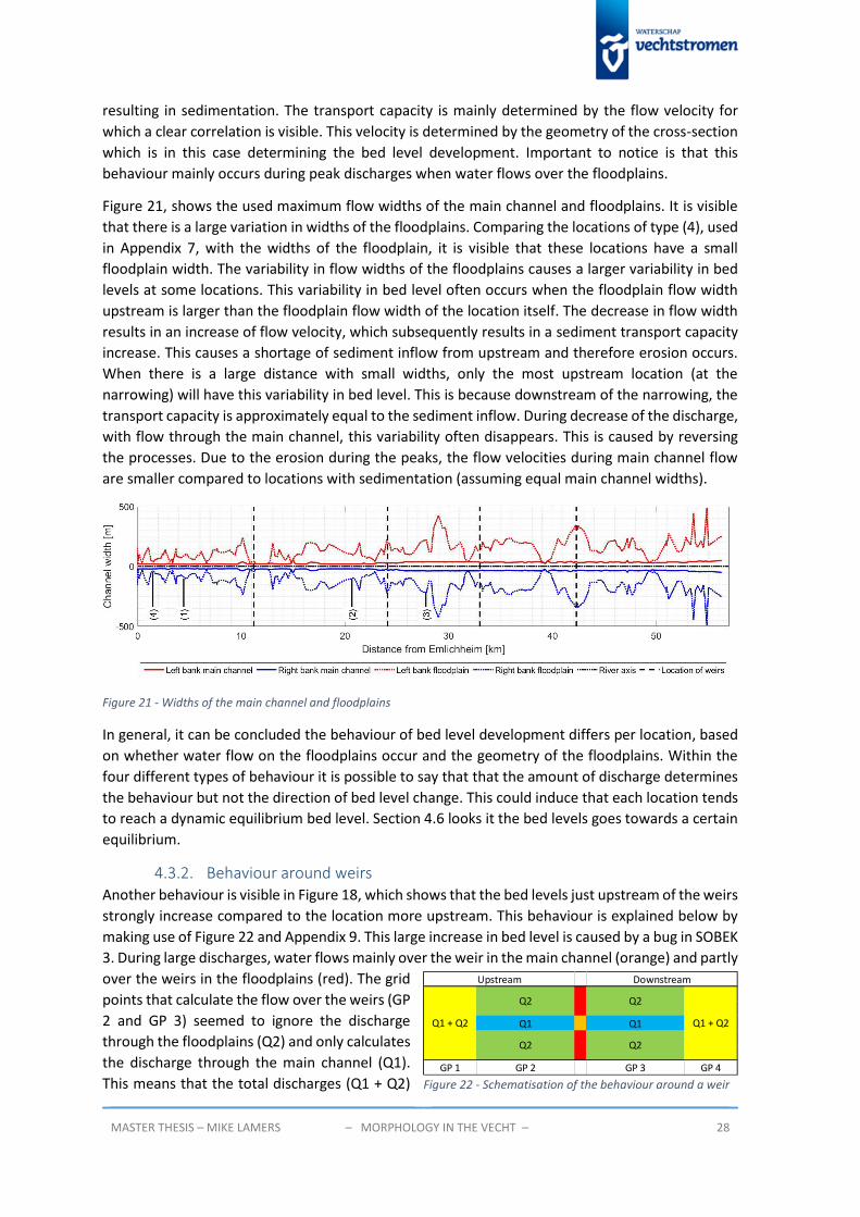
MASTER THESIS – MIKE LAMERS – MORPHOLOGY IN THE VECHT – 28
resulting in sedimentation. The transport capacity is mainly determined by the flow velocity for
which a clear correlation is visible. This velocity is determined by the geometry of the cross-section
which is in this case determining the bed level development. Important to notice is that this
behaviour mainly occurs during peak discharges when water flows over the floodplains.
Figure 21, shows the used maximum flow widths of the main channel and floodplains. It is visible
that there is a large variation in widths of the floodplains. Comparing the locations of type (4), used
in Appendix 7, with the widths of the floodplain, it is visible that these locations have a small
floodplain width. The variability in flow widths of the floodplains causes a larger variability in bed
levels at some locations. This variability in bed level often occurs when the floodplain flow width
upstream is larger than the floodplain flow width of the location itself. The decrease in flow width
results in an increase of flow velocity, which subsequently results in a sediment transport capacity
increase. This causes a shortage of sediment inflow from upstream and therefore erosion occurs.
When there is a large distance with small widths, only the most upstream location (at the
narrowing) will have this variability in bed level. This is because downstream of the narrowing, the
transport capacity is approximately equal to the sediment inflow. During decrease of the discharge,
with flow through the main channel, this variability often disappears. This is caused by reversing
the processes. Due to the erosion during the peaks, the flow velocities during main channel flow
are smaller compared to locations with sedimentation (assuming equal main channel widths).
Figure 21 - Widths of the main channel and floodplains
In general, it can be concluded the behaviour of bed level development differs per location, based
on whether water flow on the floodplains occur and the geometry of the floodplains. Within the
four different types of behaviour it is possible to say that that the amount of discharge determines
the behaviour but not the direction of bed level change. This could induce that each location tends
to reach a dynamic equilibrium bed level. Section 4.6 looks it the bed levels goes towards a certain
equilibrium.
4.3.2. Behaviour around weirs Another behaviour is visible in Figure 18, which shows that the bed levels just upstream of the weirs
strongly increase compared to the location more upstream. This behaviour is explained below by
making use of Figure 22 and Appendix 9. This large increase in bed level is caused by a bug in SOBEK
3. During large discharges, water flows mainly over the weir in the main channel (orange) and partly
over the weirs in the floodplains (red). The grid
points that calculate the flow over the weirs (GP
2 and GP 3) seemed to ignore the discharge
through the floodplains (Q2) and only calculates
the discharge through the main channel (Q1).
This means that the total discharges (Q1 + Q2) GP 1 GP 4
Q1 + Q2 Q1 + Q2
GP 2 GP 3
Upstream Downstream
Q2 Q2
Q2 Q2
Q1 Q1
Figure 22 - Schematisation of the behaviour around a weir

MASTER THESIS – MIKE LAMERS – MORPHOLOGY IN THE VECHT – 29
at GP 1 and GP 4 are larger than those of GP 2 and GP 3. Due to the decrease in discharge, the flow
velocity decreases causing sedimentation at GP 2. In Appendix 9, figures are shown containing the
water levels, bed levels, flow velocities, discharges, sediment transport capacities, flow areas and
flow widths of 1 and 2 locations upstream of the weir Hardenberg (corresponding with GP1 and
GP2 of Figure 22). The figures of Appendix 9 show the differences between the two locations during
the high discharge wave of 2033. When comparing the water levels and discharges, it is visible that
the moment of different discharges corresponds with a water level larger than the weir levels of
the floodplain which confirms the bug. This bug is present at each weir but has only (temporary)
small effects just downstream of the weirs (GP 3 and GP 4) where more erosion occurs.
4.4. Intermediate-term – Bed level development over 35 years This section contains the description of the long term morphological behaviour in the main channel
of the Vecht in the current and preferred situation after a simulation period of 35-years (2015-
2050). The bed level development until 2050 is compared with the initial situation (2015) for both
situations. The deviation from the initial bed levels of the current situation are shown in Figure 23
and of the preferred situation in Figure 25. These figures are matrices consisting of grid point
locations (on the y-axis) and the moments of the simulation period. The moment at which the
deviations are determined is the first of August each year. At that moment, bed levels are in rest
and no short term effects occur. The black dashed lines indicate the weirs in the Vecht. The
segments between these lines are the reach segments. Upstream and downstream of the Vecht
correspond with top and bottom of the figures.
4.4.1. Current situation The results of the current situation (Figure 23) show that sedimentation mainly occurs in the reach
segment Emlichheim – Haandrik. Between 0 and 3 km, erosion spots are visible after moments of
peak discharges (see Figure 18). In the beginning just downstream of De Haandrik, a large erosion
pattern is visible. This is caused by a smaller sediment inflow compared to the transport capacity of
these locations. This erosion pattern continues and grows in downstream direction and can be seen
as morphological propagation.
Figure 23 - Bed level deviations of the Vecht in current situation

MASTER THESIS – MIKE LAMERS – MORPHOLOGY IN THE VECHT – 30
However, this erosion is expected not to be caused by peak discharges as it develops over multiple
years without large peaks. Figure 24 shows that the main channel width downstream of weir De
Haandrik is much smaller than upstream, which explains the erosion pit. From 2027, bed levels start
increasing just downstream of De Haandrik. Upstream of weir De Haandrik, bed levels remain more
constant (from approximately 2030) which could indicate a dynamic equilibrium (see section 4.6)
and therefore result in more sediment transport in downstream direction. Due to this, the erosion
pits (between 10 and 13 km) are filled up slowly and grow towards its initial bed level. This
behaviour or pattern is also visible at approximately 16 till 20 km and 24 till 32 km. Several location
The larger peak discharges (2016, 2022, 2029 and 2033, see Figure 17) seems to cause more
sediment transport in downstream direction as local erosion pits occur, causing sedimentation
more downstream (large erosion pit downstream of De Haandrik). Reach segment 3, 4 and 5 are
quite stable during peak discharges except for some locations (e.g. at 22, 33 and 35 km) where
erosion pits appear and fill up over time. These pits occur due to peak discharges and small
floodplain flow widths.
Just downstream of the inflow of the Regge (at 41.2 km), the bed levels start to erode and turns to
a new constant bed level. This new bed level is probably unrealistic and underestimated because
the sediment inflow from the Regge is ignored. By comparing this with the morphological validation,
with an observation of 2013 (see Figure 16), it is assumed that the bed levels downstream of the
Regge remain approximately equal to the initial bed levels.
In general, it is clear that in the first 8 years erosion occurs mainly downstream of weirs and
continues in downstream direction which can be seen as morphological propagation of sediment
erosion. At the begin, bed levels erode quick, caused by small sediment inflow (due to large
sedimentation rates upstream) or large transport capacities (due to narrowing of the main channel)
or increase fast (due to widening of the main channel). This behaviour makes it possible to say that
the main channel width is an important parameter for the development of the bed level. Despite
the minimal sediment inflow into reach segments 3, 4 and 5, these segments are quite stable during
peaks. This could mean that the initial bed level is already in a dynamic equilibrium. This theory is
supported by comparing with reality. The (almost yearly) dredging activities that occur at de
Haandrik (at 9 km), prevent (partly) sediment transport in downstream direction resulting in
minimal inflow downstream which leads to a dynamic equilibrium bed level. If larger sediment
transport capacities would occur upstream, more incoming sediment would be transported
downstream, resulting in less erosion downstream.
Figure 24 - Main channel width of the current situation

MASTER THESIS – MIKE LAMERS – MORPHOLOGY IN THE VECHT – 31
4.4.2. Preferred alternative The bed level development of the preferred alternative is shown in Figure 25. Compared to the
current situation, reach segment 3, 4 and 5 of the preferred situation evolves in a more gradual way
and is less sensitive for peak discharges. The sediment inflow upstream is equal to those of the
current situation, which is in the preferred alternative also deposited in the upstream reach
segments. This indicates that the transport capacity at the stable, more downstream locations has
decreased. The more gradual bed deviations over the distance indicate a smaller fluctuation in
sediment transport capacity at the successive locations. Section 4.3 showed that the flow in the
main channel flattened the bed levels, therefore it is expected that the adapted cross-sections of
the preferred alternative cause the smaller deviations and a more gradual bed level compared to
the current situation. This is checked and confirmed by comparing the main channel width of the
current situation (Figure 26) with the main channel width of the preferred alternative (Figure 26).
Figure 25 - Bed level deviations of the Vecht in preferred situation
Over time, a clear propagation of sedimentation from upstream in downstream direction is visible
in reach segment 1 and 2. At the locations where mainly sedimentation take place, it is visible that
the bed levels increase quick after peak moments (2016, 2022, 2029 and 2033) and seem to reach
a certain dynamic equilibrium. The bed level increase downstream of De Haandrik is caused by small
erosion at approximately 9 km. The small sediment deposition downstream of Hardenberg (circa
23 – 26 km) is probably nourished by eroded sediment from just upstream of Hardenberg (circa 18
– 21 km and 22 – 23 km). This erosion is probably because of a decreasing main channel width,
compared to the previous width (see Figure 26. In reach segment 4 and 5, mainly downstream of
the weirs, bed level decrease occurs, which becomes larger over time and propagates in
downstream direction. The increase of bed levels at more upstream locations and the decrease of
bed levels more downstream is checked by looking at the accretion (or deposited sediment). These
figures are shown in Appendix 10. These figures also show that sedimentation more upstream
becomes less over time and that erosion stops after a certain (negative) accretion but further
propagates in downstream direction.
Downstream of the inflow of the Regge at circa 52 km, hardly any erosion occurs despite the
ignorance of sediment inflow from the Regge. It is assumed that sediment inflow from upstream is
not increased significantly with respect to the current situation, which means that the adaptation

MASTER THESIS – MIKE LAMERS – MORPHOLOGY IN THE VECHT – 32
of the main channel width is the reason for this behaviour. When sediment is transported by the
Regge, the bed level will probably increase as it is in equilibrium at this moment.
After 2050, the propagation of sediment deposition is expected to continue in downstream
direction as most bed levels upstream reach a certain dynamic equilibrium which means more
sediment will be transported to downstream locations. This is also indicated by the yellow stripe at
approximately 20 km, which is checked in the next section.
Figure 26 - Main channel width of the preferred alternative
4.5. Long-term behaviour – Towards a dynamic equilibrium bed level In previous sections it is assumed that the bed levels increase further in downstream direction over
time and that the increased bed levels are expected to reach a certain dynamic equilibrium. This is
checked below
4.5.1. Current situation and preferred alternative after 68 years This section checks these assumptions after 68 years of modelling (repeating the 35-years discharge
series) for both the current and the preferred alternative. Figure 27 shows that the initial bed levels
between Mariënberg and Junne have reached a dynamic equilibrium with the occurring amounts
of sediment inflow. However, it is visible that upstream of Mariënberg sediment is deposited and
is expected to occur between Mariënberg and Junne as well in future.
Figure 27 - Long-term development of the current situation with varying discharges
After 68 years in the preferred situation, still some sediment is deposited upstream, however this
is much less than the first 33 years. It is visible in Figure 28 that there is more sedimentation at
locations in downstream direction (between 20 and 24 km). The bed levels keep rising upstream so

MASTER THESIS – MIKE LAMERS – MORPHOLOGY IN THE VECHT – 33
after 35 years an equilibrium is not reached. Further downstream of weir Junne, still some erosion
takes place which is probably caused by too less sediment from upstream. Just downstream of
Junne, the bed level has not changed (between 35 and 68 years), which could indicate an
equilibrium in this situation. Comparing the reach segment Junne – Vilsteren of the current
situation with the preferred situation it seems that the bed level of the preferred situation tends to
reach the bed level of the current situation (which is around 0 m +NAP). This means that in the
future, when the same amount of sediment inflow upstream and discharge occurs, the bed levels
stay approximately the same. However, when no maintenance (dredging activities upstream) will
occur, bed levels will increase as well (over hundreds of years). This is because of more sediment
inflow than sediment transport capacity. This is comparable with the location at approximately 20.5
km.
Figure 28 - Long-term development of the preferred alternative with varying discharges
4.5.2. Conclusion When floodplain flow widths of floodplains suddenly decrease (in flow direction), the location with
a small width has a large variability in bed level due to an increase in flow velocity. This increase
could cause a large erosion pit, however this erosion pit is filled up during smaller discharges. Due
to the large fluctuation of floodplain flow widths in the total reach of the Vecht, the longitudinal
transect of the bed levels also fluctuates during a peak discharge. When looking only at the bed
levels during low discharges the effects of the peak discharges are disappeared often. The
behaviour of bed levels over a longer period are often related to the main channel widths. A
fluctuating width causes fluctuating bed levels. Wider main channels seem to be less sensitive for
erosion in the initial situation and therefore the bed level development of the preferred alternative
is more gradual.
Looking at the development over 35 years for both situations, the sediment is first deposited
upstream before being transported in downstream direction. The first locations with sedimentation
will move towards a dynamic equilibrium and then transport more sediment in downstream
direction. Without any maintenance, the bed level of the complete Vecht will rise between 1 and 2
meters.
4.6. Check of prerequisites The prerequisites are evaluated and should be met at each moment at each location. The
representative high water discharge T=200 (see Appendix 8) is implemented after the 35-years
discharge series. During simulation of the T=200 also bed level changes are calculated and taken
into account. The maximum water levels during the T=200 after 35 years of morphological
development are compared with the normative high water levels. These normative high water
levels are the maximum water levels during a T=200 with the initial designed bed levels (without

MASTER THESIS – MIKE LAMERS – MORPHOLOGY IN THE VECHT – 34
morphological changes). In the SOBEK 3 model, each lateral inflow has a different T=200 wave of
which the peaks occur at the same moment. Appendix 8 contains additional information about the
T = 200 discharge waves.
Figure 29 - Maximum water levels during a T = 200 with initial (2015) and evolved bed levels (2050)
Figure 29 shows the maximum water levels during a T=200 with and without bed level changes. The
increase in water levels are smaller than the increase in bed levels. This can be explained by the fact
that the lost wet area in the main channel is substituted by wet area over the total width (including
floodplains). Downstream of the weirs Mariënberg and Junne erosion took place which induced a
small water level decrease. At the most upstream reach segment, a clear increase in water level is
visible. This is caused by the large amount of sedimentation that took place. Due to bed level
changes the safety prerequisite is not met from Emlichheim until 17.5 km downstream, visible in
Figure 29. The moment when the T=200 wave takes place has influence on the simulated maximum
water levels upstream. The bed levels at that reach mainly increase over the years (seen in section
4.2.). If the T = 200 wave occurs earlier and bed levels are lower than after 35 years of development,
lower maximum water levels are expected. This is checked by comparing the maximum water levels
when implementing the T=200 wave after 1 year and 35 years. The differences are shown in Figure
30 relative to the reference maximum levels (T=200 with initial bed levels). The time of occurrence
of the T = 200 wave determines the amount of exceedance of the safe situation. The normative
water level is exceeded, which means additional measures or dredging would be required to keep
the water level below the normative level.
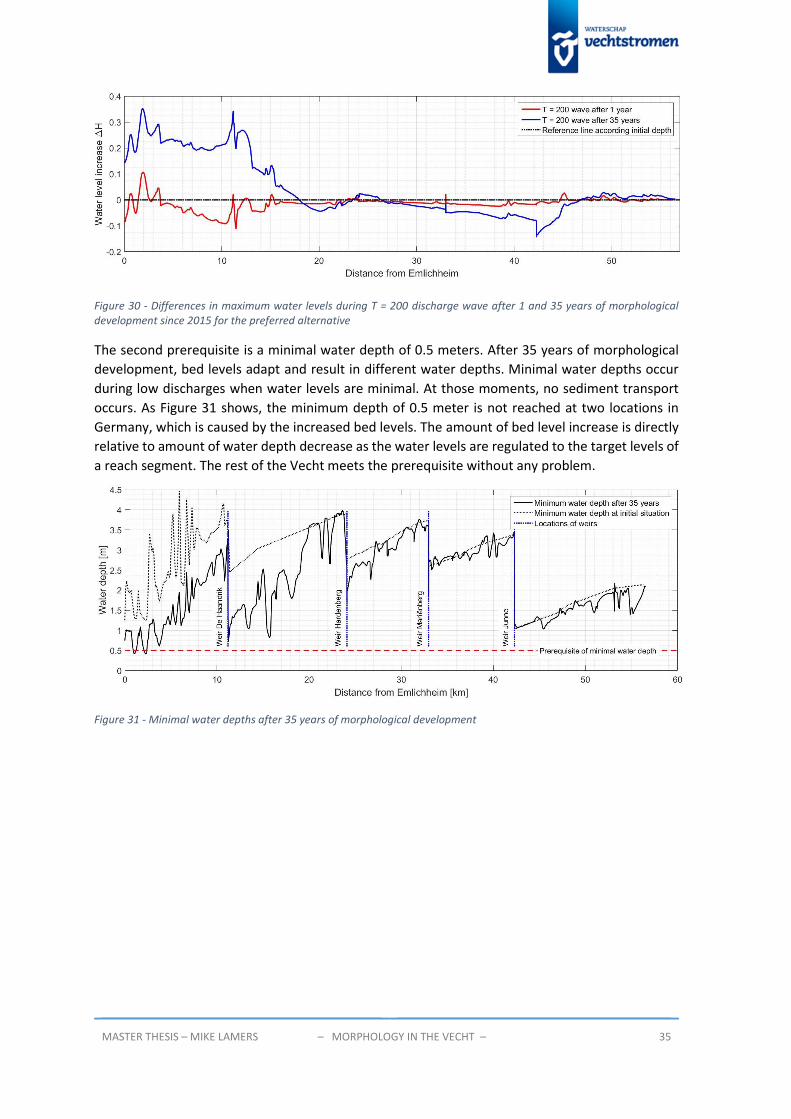
MASTER THESIS – MIKE LAMERS – MORPHOLOGY IN THE VECHT – 35
Figure 30 - Differences in maximum water levels during T = 200 discharge wave after 1 and 35 years of morphological development since 2015 for the preferred alternative
The second prerequisite is a minimal water depth of 0.5 meters. After 35 years of morphological
development, bed levels adapt and result in different water depths. Minimal water depths occur
during low discharges when water levels are minimal. At those moments, no sediment transport
occurs. As Figure 31 shows, the minimum depth of 0.5 meter is not reached at two locations in
Germany, which is caused by the increased bed levels. The amount of bed level increase is directly
relative to amount of water depth decrease as the water levels are regulated to the target levels of
a reach segment. The rest of the Vecht meets the prerequisite without any problem.
Figure 31 - Minimal water depths after 35 years of morphological development

MASTER THESIS – MIKE LAMERS – MORPHOLOGY IN THE VECHT – 36
5. Influence of measures The preferred alternative of the Vecht consist of several measures of which 2 types are evaluated
in this chapter. One type is the application of a floodplain forest on one side of the floodplains
between Mariënberg and Junne, between approximately 36.8 and 39.5 km (see Appendix 6). The
other type of measure are the 15 flood channels constructed from the old main channel of the
Vecht. The reach segments Hardenberg – Mariënberg (24.1 – 33 km) and Mariënberg – Junne (33 –
42.3 km) both contain 7 flood channels. The reach segment Junne – Vilsteren (42.3 – 56.5 km)
contains only 1 flood channel (see Appendix 6).
5.1. Methodology The influence of these two types of measures is determined by comparing the two types of
measures separately with the preferred alternative. For the simulations, the same 35-years
discharge series (2015-2050) with subsequent the T=200 discharge wave (Januari 2051) and
morphological settings (sediment inflow and transport parameter) of chapter 4 are used.
Simulation 1 – Preferred alternative, including floodplain forest and flood channels
Simulation 2 – Removal of flood channels: Preferred alternative with floodplain forest
Simulation 3 – Removal of floodplain forest: Preferred alternative with flood channels
Removing the floodplain forests means implementing a different floodplain roughness in the model
of the preferred alternative, set on a Strickler kn height of 0.2 m. Removal of the flood channels
simply means deleting these branches from the model.
The results of simulations 2 and 3 are compared with the results of the preferred alternative
(simulation 1). The following 3 aspects are compared:
Bed levels during low discharges (August 2050) and T=200 discharges (January 2051);
Minimum water depth of 0.5 meters during low discharges (August 2050);
Maximum water levels at peak of T = 200 discharge wave.
5.2. Results For the low discharges, very small differences are visible (Figure 32). The decrease of the bed levels
when removing the floodplain forests are caused during a high water event. Removing the flood
channels (indicated with numbered dashed lines in the figures) gives small differences in bed levels
during a calm situation. The deviations in bed levels at weir Mariënberg are results of bed level
changes during peak discharges.
Figure 32 - Differences in bed levels during low discharge (2050) compared to the preferred alternative

MASTER THESIS – MIKE LAMERS – MORPHOLOGY IN THE VECHT – 37
During peak discharges, differences in bed levels occur with removal of the floodplain forests. The
decrease in bed level at approximatly 19 km is not expected. When removing the flood channels, a
decrease in bed level is noticed upstream from the former flood channel. Downstream of the
former flood channel an increase of the bed level is visible. This occurs at each flood channel
(visualised by the dashed lines in Figure 33), except if flood channels are located close after each
other. The presence of a flood channel causes at the bifurcation a local increase of flow area
(transverse) and therefore a flow decceleration. This results in less sediment transport capacity and
therefore sedimentation. At the confluence a decrease of flow area is present causing a flow
acceleration and therefore erosion at that location. Without the flood channels these decellerations
and accelerations do not take place and therefore no sedimentation and erosion at the start and
end of the floodplain occur like in the preferred alternative with flood channels. After the discharge
peak, the erosion pits fill up and the peaks in bed level will be flatt again as
Figure 33 - Differences during peak discharge (2051) compared to the preferred alternative
The prerequisite of the minimum water depth is checked. Removing the floodplain forest or flood
channels induce very small differences with the preferred alternative. Like for the preferred
alternative, all locations meet the requirement of 0.5 meters except for the same two locations in
Germany (see Figure 31). This result was expected as bed levels of simulation 2 and 3 slightly differs
with simulation 1.
The last check is the impact on the maximum water levels. When removing the floodplain forests,
a decrease in maximum water level compared to the preferred alternative is obtained. This
decrease in water level starts from the most downstream part of the floodplain forest (at 36.8 km).
This means the preferred situation creates a backwater curve extending up to the weir Hardenberg
at 24.1 km. However, the effect of this measure on the increase of the water level is negligible as
the maximum difference between the preferred alternative and removal of floodplain forest is
about 1 centimetre, as shown in Figure 34.
The removal of the flood channels induces a larger increase in the maximum water levels compared
to the preferred alternative. The effect of the flood channels in the preferred alternative is a lower
water level. The absence of one flood channel between Junne – Vilsteren has minor effect.
However, excluding 14 sequent flood channels results in higher water levels because more water
will flow on the floodplains, noticing more friction. This water level increase induces a backwater
curve which reaches up till until De Haandrik (at 11.2 km). Compared to the preferred alternative,
the largest increase in maximum water level occurs at Hardenberg and is 6 centimetres.
Considering the safety prerequisite, it is possible to say that the presence or absence of the
floodplain forests in the preferred alternative has no significant effect. The number of locations that
do not meet this prerequisite does not change. The absence of flood channels creates more unsafe

MASTER THESIS – MIKE LAMERS – MORPHOLOGY IN THE VECHT – 38
situations as the maximum water levels of the reference situation are exceeded between 21.8 and
31.4 km instead of 23.5 and 26.3 km for the preferred alternative. The increase in water level ΔH is
with respect to the reference T=200 and indicates that none of the 3 simulations completely meet
the prerequisite.
Figure 34 - Effects of measures on maximum water levels during a T = 200 discharge wave, compared to the reference situation
With respect to the prerequisites, the implementation of the measures does not lead to additional
bed maintenance. Flood channels are advised because of the positive effect on lowering the
maximum water levels during a T=200 discharge wave.

MASTER THESIS – MIKE LAMERS – MORPHOLOGY IN THE VECHT – 39
6. Discussion The used flow widths of the cross-sections of the preferred alternative are taken from the hydraulic
SOBEK 2 models of the current situation. Without checking with reality, the assumption was made
that these are correct. The total flow width is however an important aspect for morphological
calculations as it has a large influence on the average flow velocities during peak discharges. The
main channel widths determine the amount of total sediment transport Qs (see Eq. ( 11 )) and are
important for bed level development (see section 4.4). The main channel width is set on the width
during bankfull discharge which could result in an over- or underestimation of the sediment
transport. Using different main channel widths could give small differences in bed level prediction.
The available discharge series are corrected and used for calibration of the hydraulic and
morphological model. The method of correction seems appropriate as the validation shows good
agreements in both shape and amounts and therefore this correction was useful for calibration.
The sediment inflow from laterals is not taken into account as it is assumed to be minimal. Section
3.5 shows that mainly the Regge is expected to transport sediments into the system as the bed level
is underestimated. This underestimation has hardly effects on bed level development of upstream
locations and is therefore not further corrected.
Close to weirs severe sedimentation and erosion is noticed during peak discharges. This behaviour
is caused by a bug in SOBEK 3 (see section 4.3.2) and is ignored as it has only little impact on bed
levels downstream during the peak discharge. After the peak, the deposited sediment is
transported over the weir and do not affect long term bed level development.
The calibration results of the sediment inflow and transport parameter are slightly uncertain, as the
calibration took place over only 5 years (2008-2013). These results are the best approximation.
Assuming the sediment inflow is overestimated, this would also result in sedimentation upstream,
but slower as before. The sedimentation continues until the same dynamic equilibrium level is
reached. The propagation speed of sedimentation in downstream direction will decrease which
means that the erosion processes downstream will also continue longer. This means that erosion
spots will reach an equilibrium depth and meanwhile propagate in downstream direction until there
is more sediment inflow. When the sediment inflow would be underestimated, the sedimentation
processes upstream will occur quicker, and therefore also an earlier propagation of deposited
sediment in downstream direction and less erosion downstream. A different transport parameter
will induce a different dynamic equilibrium level but also different propagation of deposited
sediment in downstream direction.

MASTER THESIS – MIKE LAMERS – MORPHOLOGY IN THE VECHT – 40
7. Conclusion and recommendations
7.1. Conclusion Migrating the original SOBEK 2 models into SOBEK 3 models, adapting cross-sections and correcting
discharges, resulted in a calibrated hydraulic model of the main channel with an average RMSE of
0.08, which makes it useful for calibration of the morphological parameters. The calibration of the
floodplain roughness showed that the water levels insensitive for the roughness height. This
indicates that average flow velocities are approximately equal for different roughness heights and
therefore this calibration is not very important for morphological calculations. The roughness
heights of the SOBEK 2 model are used.
The morphological calculations are performed with the formula of Engelund and Hansen (1967).
This choice is based on the characteristics of the Vecht that proved to be within the range of
application for the type of load, sediment diameter and a Shields parameter.
The morphological calibration resulted in a sediment inflow at the upstream boundary of 30 % of
the sediment transport capacity and a transport parameter α of 0.75. With the uncertain 35-years
discharge series the long term behaviour can be predicted. Short term behaviour is more
dependent on the occurring discharges and therefore less certain to predict.
Obtaining all calibration parameters and a 35-years discharge series the main research question can
be answered:
Where and in what order of magnitude will morphological processes as sedimentation and erosion
change due to implementing the preferred alternative of the Vecht and what consequences does it
have on maintenance?
After modelling the current situation and the preferred alternative over 35 years, it is visible that
the Vecht is a quite morphological active river, which yearly average transport between 1200 and
15000 m3/s, depending on the location. In the current situation and in the preferred alternative,
inflowing sediment starts depositing upstream between Emlichheim and De Haandrik. Peak
discharges seem to stimulate more sediment transport in downstream direction. Bed levels during
low discharges show hardly the effects of peak discharges. The bed levels during low discharges are
related to the main channel widths. In the current situation there are more locations with stronger
erosion (2 meters), caused by smaller main channel widths compared to the preferred alternative
(maximum 1 meter). A large erosion pit downstream of De Haandrik of about 2 meters deep and 2-
3 km long is a good example. The preferred alternative is more stable, due to wider main channels,
causing smaller sediment transport capacities.
During peak discharges, short-term morphological behaviour arise which is not depending on the
main channel width but by the flow width of the floodplains. Decreasing floodplain widths (in flow
direction) induce an increase in flow velocity causing larger sediment transport capacities. Large
fluctuations in floodplain widths cause large variability in bed levels with often large erosion pits.
When these peak discharges decreases, the erosion pits fill up due to less fluctuating main channels.
As the floodplain widths do not change, the short-term behaviour of the current situation is
comparable to the behaviour of the preferred alternative.
For both the current situation as the preferred alternative, the bed level development between
Emlichheim and De Haandrik seemed to go towards a dynamic equilibrium when comparing an
additional run of 68 years with the run of 35 years. The difference in bed levels between 35 and 68
years are quite small and sediment deposition is propagating more in downstream direction. Based

MASTER THESIS – MIKE LAMERS – MORPHOLOGY IN THE VECHT – 41
on the bed level development after 68 years, it is expected that when no maintenance is applied,
all bed levels of the Vecht will be increased with approximately 1 till 2 meters after a couple of
hundred years. Between Mariënberg and Vilsteren, the bed levels of the current situation are more
stable due to earlier erosion. The new designed bed levels of the preferred alternative erode
towards the bed heights of the current situation.
The prerequisites for safety and recreational navigation are checked. The minimal water depth of
0.5 meter is met at all locations in the area of water board Vechtstromen. After 35 years of bed
level development, without dredging activities, bed levels increase between Emlichheim and
approximately 18 km downstream (of which 10 km belongs to Vechtstromen), resulting in an
exceedance of the maximum water levels up to 30 cm. The exceedance already starts after one year
and increase over time. To keep the maximum water level at the normative level it is required to
dredge on a regular basis, which is done already almost each year (Vogelsang, 2016). This prevents
further deposition of sediment more downstream. The dredged materials can be put back into the
river more downstream in erosion pits or other locations. This sediment will again be transported
downstream without causing problems.
The two studied measures, flood channels and floodplain forest, have only impact during higher
discharges. During peak discharges, the 15 flood channels cause differences in bed level at the
bifurcation and confluence of the flood channel, which will disappear after the peak discharge. The
floodplain forests have hardly effect on the bed levels. Both measures have no effect on the
maximum water levels or water depths, caused by changing bed levels, and therefore need no
additional maintenance.
7.2. Recommendations For morphological modelling in SOBEK 3
During simulations one very important aspect in the SOBEK 3 model was discovered. To calculate
morphological, it is required to have a grid point between a structure and the begin or end node of
a branch. In the initial network of the SOBEK 3 model of the preferred alternative this was not the
case and the model was not able to update the bed level and resulted in simulation failure.
SOBEK 3 automatically calculates time steps to obtain a stable numerical model by having a Courant
number smaller than 1. However, sometimes this results into too small time steps leading to failure
of the model. This is solved by examining the grid points and adapting them into a stable situation.
The model contains 4 weirs, regulated with the PID controller. When the target level suddenly
changes from winter to summer level or the other way around, the model has some hydraulic
disturbance which resulted in a major morphological disturbance with some unrealistic bed level
changes. These problems occurred due to sudden changes in crest levels of the weirs. This effect is
dealt with by imposing a gradual change in crest level with one centimetre per time step instead of
the complete difference in one time step. These strong disturbances were mainly encountered at
Junne.
Successive branches in the model need a specific order number (not equal to the default value), to
prevent large bed level differences at nodes (up to 1.5 meters). SOBEK 3 normally interpolates
between the cross-sections, however when successive branches do not have a specific order
number, the sediment transport is calculated between a cross-section and the end or start node of
the branch causing a jump in bed level at the nodes connecting successive branches.

MASTER THESIS – MIKE LAMERS – MORPHOLOGY IN THE VECHT – 42
For Water board Vechtstromen
Recommendations with respect to future policy are regarding monitoring the bed levels to validate
and possibly improve the morphological model. Only 3 bed level measurements were available to
calibrate the sediment inflow and transport parameter with. Upcoming years bed levels should also
be monitored just after peak discharges at locations that are sensitive to peak discharges, to check
the implemented transport parameter. On a yearly basis, during low discharges, bed levels should
be monitored and compared with results of morphological simulations. If possible, it would be very
useful to monitor sediment inflow which could be compared with the calibrated infow,
corresponding to the same discharge.
It is highly recommended to check all measurement stations and their Q-H relations. Based on the
checks, the relations or stations should be adapted resulting in a better water balance for the Vecht.

MASTER THESIS – MIKE LAMERS – MORPHOLOGY IN THE VECHT – 43
References Deltares, 2013a. 1D/2D modelling suite for integral water solutions; Hydrodynamics; Technical
Reference Manual. Version: 3.0.1.29298, 30 July 2013.
Deltares, 2013b. Software tools for modelling real-time control; RTC-Tools; Technical Reference
Manual. Version: 0.7.28889, 30 July 2013.
DHV, NWP Planungsgesellschaft mbH (2009). DE VECHT een grenzeloze, halfnatuurlijke rivier -
grensoverschrijdende vechtvisie. Retrieved from: www.devecht.eu.
Engelund, F. & Hansen, E. (1967). A monograph on sediment transport in alluvial streams. Tenisk
Forlag, Kopenhagen
Graaff, B., Groot, S., Termes, P. (2008). Concrete uitwerking van de Reggevisie, van verzamelleiding
tot meanderende rivier. HKV Lijn in water
Mosselman E., van der Mark R. (2009). Tussenevaluatie ontstening Vechterweerd, 1201579-000.
Delft: Deltares
Province Overijssel, 2009. Masterplan Ruimte voor de Vecht.
http://www.overijssel.nl/thema's/water/waterprojecten/ruimte-vecht/
Ribberink, J.S., Hulscher, S.J.M.H., (2012). Lecture Notes River Dynamics – I: Shallow-water flows,
course id: 195400400. Univerisity of Twente, p. 2.26-2.32
Ribberink, J.S., (2011). Lecture Notes River Dynamics – II: Transport processes and Morphology,
course id: 195400400. Univerisity of Twente, p. 2.16-2.20, 4.36, 7.71,
Rijn, L.C. van, (1993). Principles of sediment transport in rivers, estuaries and coastal areas.
Oldemarkt: Aqua publications. -I11, ISBN 90-6562-146-6
Scheer, J. van der (2015). Oppervlaktewatermodellering Vecht – Achtergrondrapport bij
Ruralmodel. Last modification: 29-07-2015. Waterschap Vechtstromen
Toorn, L. van der (2016). Scenariobeschrijving Plan op hoofdlijnen Vecht. Water board
Vechtstromen. Last modified on: 14-12-2016;
Van der Mheen, M., Keizer, A., & de Jong, J. (2015). SOBEK 3-model van de Overijsselse Vecht,
1220072-006. Delft: Deltares.
Vogelsang, L. G., (2016). River governance as a major component of the riverine sediment regime -
A case study on the transboundary Vecht River. Vechtstromen and Wageningen University. Master
thesis.
Wang, Z., R. Fokkink, M. D. Vries, and A. Langerak (1995). Stability of river bifurcations in 1D
morphodynamic models, J. Hydraul. Res., 33(6), 739– 750
Wolfert, H., Corporaal, A., Maas, G., Maas, K., Makaske, B. & Termes, P. (2009a). Herstelonderzoek
Vecht. Alterra Wageningen.
Wolfert, H., Corporaal, A., Maas, G., Maas, K., Makaske, B. & Termes, P. (2009b). Toekomst van de
Vecht als een halfnatuurlijke laaglandrivier; Bouwstenen bij de grensoverschrijdende Vechtvisie.
Wageningen
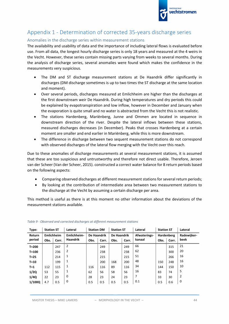
MASTER THESIS – MIKE LAMERS – MORPHOLOGY IN THE VECHT – 44
Appendix 1 - Determination of corrected 35-years discharge series Anomalies in the discharge series within measurement stations The availability and usability of data and the importance of including lateral flows is evaluated before
use. From all data, the longest hourly discharge series is only 18 years and measured at the 4 weirs in
the Vecht. However, these series contain missing parts varying from weeks to several months. During
the analysis of discharge series, several anomalies were found which makes the confidence in the
measurements very suspicious.
The DM and ST discharge measurement stations at De Haandrik differ significantly in
discharges (DM discharge sometimes is up to two times the ST discharge at the same location
and moment).
Over several periods, discharges measured at Emlichheim are higher than the discharges at
the first downstream weir De Haandrik. During high temperatures and dry periods this could
be explained by evapotranspiration and low inflow, however in December and January when
the evaporation is quite small and no water is abstracted from the Vecht this is not realistic.
The stations Hardenberg, Mariënberg, Junne and Ommen are located in sequence in
downstream direction of the river. Despite the lateral inflows between these stations,
measured discharges decreases (in December). Peaks that crosses Hardenberg at a certain
moment are smaller and end earlier in Mariënberg, while this is more downstream.
The difference in discharge between two sequent measurement stations do not correspond
with observed discharges of the lateral flow merging with the Vecht over this reach.
Due to these anomalies of discharge measurements at several measurement stations, it is assumed
that these are too suspicious and untrustworthy and therefore not direct usable. Therefore, Jeroen
van der Scheer (Van der Scheer, 2015). constructed a correct water balance for 8 return periods based
on the following aspects:
Comparing observed discharges at different measurement stations for several return periods;
By looking at the contribution of intermediate area between two measurement stations to
the discharge at the Vecht by assuming a certain discharge per area.
This method is useful as there is at this moment no other information about the deviations of the
measurement stations available.
Table 9 - Observed and corrected discharges at different measurement stations
Type: Station ST Lateral Station DM Station ST Lateral Station ST Lateral
Return period
Emlichheim Emlichheim-Haandrik
De Haandrik De Haandrik Afwaterings-kanaal
Hardenberg Radewijker-beek Obs. Corr. Obs. Corr. Obs. Corr. Obs. Corr.
T=200 247 2 249 249 66 315 21
T=100 236 2 238 238 62 300 20
T=25 214 1 215 215 51 266 16
T=10 199 1 200 168 200 48 150 248 16
T=1 112 115 1 116 116 89 116 34 144 150 10
1/2Q 53 55 1 62 56 58 56 16 83 74 5
1/4Q 22 23 0 28 23 24 23 7 33 30 2
1/100Q 4.7 0.5 0 0.5 0.5 0.5 0.5 0.1 0.5 0.6 0

MASTER THESIS – MIKE LAMERS – MORPHOLOGY IN THE VECHT – 45
Type: Station ST Lateral Station ST Lateral Station DM Lateral Station ST
Return period
Mariënberg Mariënberg-Vechtkanaal
Junne Junne- Ommenbrug
Ommenbrug Ommerkanaal and Regge
Vilsteren
Obs. Corr. Obs. Corr. Obs. Corr. Corr.
T=200 336 11 347 8 355 145 500
T=100 320 10 330 8 338 140 478
T=25 284 9 293 7 300 120 420
T=10 186 264 8 532 272 7 194 279 105 384
T=1 156 160 5 287 165 4 167 169 70 239
1/2Q 72 79 3 81 82 2 84 84 37 121
1/4Q 31 32 2 32 34 1 35 35 18 53
1/100Q 0.2 0.6 0 0.2 0.6 0.1 1.7 0.7 1.7 2.4
The results of this approach are shown in Table 2 which contains the observed (Obs.) and corrected
(Corr.) discharges [m3/s] for the measurement stations located in the Overijsselse Vecht. The columns
left to right are the sequence in downstream direction. Based on the available observed data, the
corresponding discharges for several return periods T are determined. As the available data is limited
to maximal 10 years, the very high corrected discharges (T=25, T=100 and T=200) are determined by a
theoretical ratio executed by Jeroen van der Scheer (Scheer, 2015). This way of extrapolating should
be done with a Gumbel, Weibull or Gringorten formula instead of a theoretical ratio.
Table 2 shows several aspects that agree with the earlier mentioned anomalies. Emlichheim has very
high observed discharges during lower discharges compared with all other measurement stations. It is
assumed these discharges are estimated too high and are corrected. The other return periods show
good agreement between observed and corrected discharges. At De Haandrik DM higher discharges
are observed than at De Haandrik ST. The low discharges agree well, but high discharges (at T=1 and
T=10) are underestimated by De Haandrik ST. Hardenberg observes to low discharges during very high
(T=10) discharges, which are almost equal to the discharge at T=1. The next measurement station at
Junne observes too high discharges during the larger return periods T=1 and T=10. On the other hand,
the observed very high discharges at Ommenbrug are way too low. The incorrectness of the observed
data makes it necessary to correct it for the total measurement length.
Beside the incorrectness of the observations, also the measurement period of the discharges at the
weirs and lateral inflows are too short (18 years) to obtain a discharge series of 35 years. This length is
required as the goal is to simulate morphological behaviour with realistic discharges over 35 years. As
only Emlichheim has this length of measurements, the new discharge series for the inflow upstream is
based on the correction of the 35-year long observed discharges at Emlichheim. The lateral inflow
between each weir is determined by the difference between the corrected discharges of the weirs up-
and downstream of that lateral. Only Emlichheim has measurements from 1980 until 2015, to obtain
35 years of data. These measurements consist of:
Water levels, measured daily from 1980 till 2009 and hourly from 2009-2015.
Discharges, derived from Q(H) relation, daily from 1990 till 2009 and hourly from 2009 till 2015.
Before correcting the discharge series, the missing discharges (1980-1990) have to be derived similar
as the available discharge series is too small. This is done in the next section.

MASTER THESIS – MIKE LAMERS – MORPHOLOGY IN THE VECHT – 46
Determination of 35-years discharge series The missing discharges at Emlichheim between
1980 and 1990 are computed similar like the
computed discharge series for the period 1990-
2005. These are computed with a Q(H) relation
The Q(H) relation of 2009-2015 is shown by the
trend line (red line) through the Q-H graph
which is visible in Figure 35. To have the same
estimation precision as used for the period
1990-2015, a polynomial function of the third
power for the trend line is used, generalised by
Eq. ( 12 ).
General function: 𝑌 = 𝑎 ∙ 𝑋3 + 𝑏 ∙ 𝑋2 + 𝑐 ∙ 𝑋 + 𝑑 Eq. ( 12 )
The daily discharges between 2009 and 2015 are determined with a Q(H) relation, which explains the
nice reproduced Q(H) relation of Figure 35. As the discharges are missing and water levels are known,
the Q(H) relation is determined. The values for the parameters a,b,c and d are shown in Table 10.
Table 10 - Parameter values Q-H and H-Q relation
Relation Y X a b c d
Q(H) relation Q H 0.1902 -0.6114 -13.7020 34.2443
To complete the 35-years hourly discharge series, the daily water levels (1980 – 1990) are filled in Eq.
( 12 ) with the parameters from Table 10 and the daily discharges (1980-2009) are interpolated with
the cubic interpolation method which gives a smooth interpolation with only positive values.
Correction of discharges As mentioned before, the measured discharges at Emlichheim are quite high compared to
measurements from other measurement stations downstream of Emlichheim. Deltares also noticed
during the calibration of their SOBEK 3 model of the Vecht (part of a larger system) that the discharges
at Emlichheim are quite high which corresponds to these findings (Van der Mheen et al., 2015). Jeroen
van der Scheer (water board Vechtstromen) already derived corrected discharges at the different weirs
and measurement stations located in the Vecht. Table 2 contains the corrected discharges for each
station for several return periods.
Figure 36 – Exceedance frequencies
Figure 35 - Q-H relation 2009 – 2015 at Emlichheim

MASTER THESIS – MIKE LAMERS – MORPHOLOGY IN THE VECHT – 47
These corrected discharges with a certain return period can be transformed into an exceedance
frequency line, which shows the discharge corresponding to a certain frequency of occurrence. This is
visible in Figure 36 by the red dashed line.
To make a best guess of the true discharges at Emlichheim it is assumed that the observed discharges
should follow the exceedance frequency line of the corrected discharges at Emlichheim. The
exceedance frequency line of the observed discharges at Emlichheim can also be made and scaled
towards the exceedance frequency line of the corrected discharges. This can be done as follows:
1. The discharges from the series 1980-2015 with the corresponding dates, can be sorted from
large to small.
2. The smallest discharge is always exceeded and has therefore a frequency F0 of 8760 hours a
year (the whole year). The frequencies for the other discharges are determined with the
following formula:
Smallest discharge 𝐹0 = 𝑁 = # of hours per year = 8760
Arbitrary discharge 𝐹𝑛 = 𝐹0 − 𝑛 ∗𝑁
𝑀
Highest discharge 𝐹𝑁 = 𝐹0 − (𝑀 − 1) ∗𝑁
𝑀
M is the total amount of observed moments of the series; for 35-years hourly observations it gives 315574 discharge values.
3. For these frequencies, the corresponding corrected discharges are determined by
interpolating between the corrected discharges of Table 2.
4. As each frequency corresponds to a certain date, the determined discharges are sorted on
ascending dates.
In this way real discharges are scaled to the corrected discharges. This is done with the same
frequencies for all measurement stations of Table 2. The correction of the inflow at Emlichheim is
shown in Figure 37. When comparing the corrected with the observed discharges for the period June
2008 until June 2009, it is visible that the corrected discharge follows the shape of the observed
discharges. The corrected discharges are slightly smaller at the peaks and significantly smaller for small
observed discharges which corresponds with Table 2.
Figure 37 - Corrected vs observed discharges
As there are corrected discharges for each measurement station, discharges from lateral flows
(between the weirs) can be determined by subtracting the corrected discharge of the downstream
weir from the corrected discharge of the upstream weir. For each river segment it is possible to link

MASTER THESIS – MIKE LAMERS – MORPHOLOGY IN THE VECHT – 48
this difference with a lateral flow except between Junne and Vilsteren as there are two significant
lateral flows, namely the Regge and the Ommerkanaal. To determine the contribution of these two
lateral flows to the Vecht, the fraction R of the total inflow between Junne and Vilsteren that is
contributed to the Regge is calculated. This is done by looking at measured discharges at the Regge
and Ommerkanaal over the years 2005 and 2006 (Figure 38) and taking the fraction R:
Fraction of the Regge: 𝑅 =1
𝑛∗ ∑
𝑄𝑅𝑒𝑔𝑔𝑒
𝑄𝑅𝑒𝑔𝑔𝑒 + 𝑄𝑂𝑚𝑚𝑒𝑟𝑘𝑎𝑛𝑎𝑎𝑙= 0.8665
𝑛
𝑖=0
Eq. ( 13 )
The inflow contributed to the Ommerkanaal is the total inflow minus the contribution of the Regge.
Figure 38 - Discharges of the Regge and the Ommerkanaal

MASTER THESIS – MIKE LAMERS – MORPHOLOGY IN THE VECHT – 49
Appendix 2 – Calibration results main channel

MASTER THESIS – MIKE LAMERS – MORPHOLOGY IN THE VECHT – 50
Appendix 3 – Calibration of the floodplain

MASTER THESIS – MIKE LAMERS – MORPHOLOGY IN THE VECHT – 51
Appendix 4 – Validation results

MASTER THESIS – MIKE LAMERS – MORPHOLOGY IN THE VECHT – 52
Appendix 5 – Calculations for check suitability of Engelund and Hansen Grain diameter
The range of grain diameter of the Vecht is between 0.3 and 0.35 mm (Wolfert et al., 2009a), resulting
in an average grain diameter of 0.325 mm. This is within the validity range of 0.19 and 0.93 mm.
Shields parameter
The Shields-parameter is a measure of the mobility of sediment. This mobility is related to a minimum
and maximum bed shear velocity, which can be transformed into a flow velocity. This is done by using
the formula of the Shields-parameter 𝜃 [−], Eq. ( 14 ) and the formula of the bed shear velocity [m/s]
Eq. ( 15 ):
Shields-parameter 𝜃 [-] 𝜃 =𝑢∗
2
𝑔 ∗ ∆ ∗ 𝐷50 𝑤𝑖𝑡ℎ ∆ =
𝜌𝑠 − 𝜌
𝜌 Eq. ( 14 )
Bed shear velocity [m/s] 𝑢∗ = 𝑢 ∗√𝑔
𝐶 Eq. ( 15 )
Transforming the bed shear velocity 𝑢∗ [m/s] into the flow velocity u [m/s], the Shields formula is
transformed as follows:
𝜃 =
(𝑢 ∗√𝑔𝐶 )
2
𝑔 ∗ ∆ ∗ 𝐷50=
𝑢2 ∗ 𝑔
𝑔 ∗ ∆ ∗ 𝐷50 ∗ 𝐶2 𝑟𝑒𝑤𝑟𝑖𝑡𝑡𝑒𝑛 𝑎𝑠: 𝑢 = √𝜃 ∗ (
𝜌𝑠 − 𝜌
𝜌) ∗ 𝐷50 ∗ 𝐶2
Parameter Symbol Value Unit Gravitational acceleration g 9.81 m/s2 Grain density ρs 2650 kg/m3 Water density ρ 1000 kg/m3 Grain diameter D50 0.000325 m Chézy coefficient C 31 m1/2/s Minimum shields 𝜃 0.07 - Maximum shields 𝜃 6 - viscosity (at 10 °C) ν 1.307 * 10-6 m2/s
When filling in the above parameters, a minimal and maximal flow velocities of 0.19 and 1.76 m/s
respectively are obtained. The maximum velocity will never be exceeded. The minimum velocity will
exceed during low discharges as the Vecht is a dammed river.
Total load
Sediment is brought into suspension if the driving force (bed shear velocity 𝑢∗ [m/s]) is larger than
the resisting force (fall velocity of a grain 𝑤𝑠 [m/s]) (Ribberink, 2011). The fall velocity 𝑤𝑠 is
determined by Eq. ( 16 ), a formula of Van Rijn (1993), and the above parameters:
Fall velocity [m/s] (100 < D50 < 1000 μm)
𝑤𝑠 =10𝑣
𝐷50(√1 +
0.01∆𝑔𝐷503
𝑣2− 1) Eq. ( 16 )
This gives a fall velocity ws of 0.043 m/s. The grains will be brought into suspension if 𝑢∗ > 𝑤𝑠 which
requires a minimum depth-averaged flow velocity u of 0.426 m/s. This depth averaged flow velocity
certainly occurs in reality.

MASTER THESIS – MIKE LAMERS – MORPHOLOGY IN THE VECHT – 53
Appendix 6 – Measures of the preferred alternative
Reach segment 1
Reach segment 2
Reach segment 3
Reach segment 4
Reach segment 5
Legend
") Boundary
&3 Lateral inflow
Weirs
Flood channels
Main channel preferred alternative
Main channel current situation
Floodplain forest
Ü

MASTER THESIS – MIKE LAMERS – MORPHOLOGY IN THE VECHT – 54
Appendix 7 – Different locations for each type

MASTER THESIS – MIKE LAMERS – MORPHOLOGY IN THE VECHT – 55
Appendix 8 – T = 200 discharge waves The normative high water discharges at the different measurement stations are determined with a
uniform wave. These waves have a minimum and maximum discharge corresponding respectively with
the discharges of a ¼ Q and T = 200 return period (Table 9 in Appendix 1). The discharges of the lateral
inflows are determined by subtracting the upstream discharge wave from the downstream discharge
wave. The discharge waves at the measurement stations and later inflows are visible in respectively
Figure 39 and Figure 40.
Figure 39 - Design Wave T = 200 at measurement stations
Figure 40 - Discharge waves of lateral sources
0.00
100.00
200.00
300.00
400.00
500.00
600.00
Dis
char
ge Q
[m
3/s
]
Date
Design discharges T = 200
Emlichheim
De Haandrik
Hardenberg
Marienberg
Junne
Ommenbrug
Vilsteren
0.00
20.00
40.00
60.00
80.00
100.00
120.00
140.00
Dis
char
ge Q
[m
3/s
]
Date
Lateral inflows
Emlichheim_Haandrik
Afwateringskanaal
Radewijkerbeek
Marienberg-Vechtkanaal
Junne_Ommenbrug
Regge
Ommerkanaal

MASTER THESIS – MIKE LAMERS – MORPHOLOGY IN THE VECHT – 56
Appendix 9 – Analysis of behaviour in front of weir Hardenberg

MASTER THESIS – MIKE LAMERS – MORPHOLOGY IN THE VECHT – 57
Appendix 10 – Total sediment transport and accretion on 6 moments