Embed Size (px)
Citation preview
i
Analysing the Requirements for Monitoring and Switching: A Problem-Oriented Approach
Mohammed Salifu BSc (Hons), MSc
A thesis submitted in partial fulfilment of the requirements for the degree of Doctor of Philosophy in Computing
Department of Computing Faculty of Maths, Computing and Technology
The Open University
2008

ii
iii
Abstract
Context-aware applications monitor changes in their environment and switch their behaviour
in order to continue satisfying requirements. Specifying monitoring and switching in such
applications can be difficult due to their dependence on varying environmental properties. Two
problems require analysis: the detection of changes in the operating environment to assess their
impact on requirements satisfaction, and the adaptation of application behaviour to ensure
requirements satisfaction.
This thesis borrows from the world of problem-oriented software system development and
product-lines to analyse monitoring and switching problems on one hand and contextual
changes on the other. It proposes a shift of focus from treating monitoring and switching as
activities to be analysed as part of the design, to treating them as part of the problem whose
requirements are analysed. We claim three novel contributions: (1) we provide concepts and
mechanisms for analysing monitoring and switching problems in context; (2) we formulate and
prove two theorems for monitoring and switching, which define the necessary and sufficient
conditions for monitoring a contextual variable and for switching application behaviour to
restore requirements satisfaction when they are violated; and (3) we provide a tool for
automated derivation of the conditions for monitoring and switching.
Our approach is evaluated using two case studies of a proof of concept mobile phone product-
line and a logistics company that delivers and monitors products across the UK. We found the
applications of the approach to be effective in analysing unforeseen requirements violations
caused by changes in the systems operating environments. Furthermore, the monitoring and
switching mechanisms derived from the analysis enabled the software to become, to some
extent, context-aware.

iv

v
Acknowledgements
The work presented in thesis was made possible by the invaluable support and guidance my
supervisors Bashar Nuseibeh and Yijun Yu provided to me. I will forever be very grateful for
the role they played in ensuring that I finish this thesis. I wish to thank Lucia Rapanotti for the
guidance and encouragement during the early stages of my studies; and Michael Jackson for his
support and feedback that contributed in shaping the direction of this research.
To my family, a special thanks to: my beloved wife Jola Salifu for her love, patience,
understanding and continous support during this difficult process; my unborn son for keeping
his mother occupied and accompanied when my studies took me away from her and for giving
me the greatest motivation to get on with the work; and to my dad and mum for recognising the
value of education and for offering me an opportunity they never had themselves.
Finally, I acknowledge the support of other members of The Computing Department of The
Open University without which my experiance with the university would have been less
fulfilling.

6
7
Table of Contents
Chapter 1. Introduction .................................................................................................................13
1.1 Research Questions ............................................................................................................14
1.2 Objectives and Contributions ..............................................................................................16
1.3 Research Methodology .......................................................................................................17
1.4 Structure of the Thesis ........................................................................................................18
Chapter 2. Related Work ...............................................................................................................19
2.1 Basic Concepts and Definitions...........................................................................................19
2.1.1 Operating Environment as Application Context ............................................................. 19
2.1.2 Self-Managing and Context-Awareness ......................................................................... 23
2.1.3 Requirement and Specification ...................................................................................... 23
2.1.4 Problem-Oriented and Solution-Oriented Approaches ................................................... 24
2.1.5 On the Notion of Variability .......................................................................................... 26
2.1.6 Software Monitoring and System Monitoring................................................................. 26
2.1.7 Software Switching and System Switching...................................................................... 27
2.1.8 Deployment-Time Switching and Run-Time Switching ................................................... 27
2.1.9 Dependency and Context............................................................................................... 28
2.2 Problem Description for Requirements Analysis .................................................................28
2.3 Variability Analysis............................................................................................................30
2.3.1 Eliciting Variability....................................................................................................... 31
2.3.2 Modelling Variability and Selecting Variants................................................................. 33
2.4 Monitoring and Switching Requirements ............................................................................38
2.4.1 Requirements Inconsistency........................................................................................... 38
2.4.2 Failure Diagnostics....................................................................................................... 39
2.4.3 Testing and Maintenance .............................................................................................. 40
2.4.4 Performance Tuning ..................................................................................................... 40
2.4.5 Ubiquitous Computing .................................................................................................. 41
2.4.6 Self-Managing .............................................................................................................. 41
2.4.7 Other Works ................................................................................................................. 42
2.5 Automated Analysis Support ..............................................................................................43
8
2.5.1 Support for Variability Analysis .................................................................................... 43
2.5.2 Support for Monitoring and Switching Analysis ............................................................. 44
2.6 Chapter Summary...............................................................................................................47
Chapter 3. Analysing Problems for Different Contexts.................................................................49
3.1 Facilitating Example...........................................................................................................50
3.2 Variability in Application Contexts .....................................................................................50
3.3 Variability in Problem Descriptions ....................................................................................53
3.4 Problem Descriptions for Different Contexts .......................................................................54
3.5 Dependency in Problem Descriptions..................................................................................58
3.6 A Comparative Study .........................................................................................................60
3.7 Chapter Summary...............................................................................................................66
Chapter 4. Analysing Monitoring and Switching Problems..........................................................67
4.1 Monitoring Problems ..........................................................................................................67
4.1.1 Direct Monitorable Variables........................................................................................ 69
4.1.2 Indirect Monitorable Variables ..................................................................................... 70
4.2 Switching Problems............................................................................................................72
4.3 Theorems for Monitoring and Switching Conditions ...........................................................74
4.3.1 Requirements Satisfaction and Constraints Satisfiability................................................ 75
4.3.2 Proofs for our Monitoring and Switching Theorems....................................................... 77
4.4 A Comparative Study .........................................................................................................79
4.5 Chapter Summary...............................................................................................................81
Chapter 5. Automated Analysis Using Constraint Satisfiability ...................................................83
5.1 Monitored Variables ...........................................................................................................88
5.1.1 Alogrithm for Eliciting Monitored Variables.................................................................. 88
5.1.2 Algorithms for Ranking Monitored Variables................................................................. 90
5.2 Monitoring Conditions........................................................................................................91
5.2.1 Implementing the Necessary Monitoring Condition as Defined by our Theorem1 ........... 91
5.2.2 Algorithm for Deriving Necessary Monitoring Conditions ............................................. 92
5.3 Switching Conditions..........................................................................................................93
5.3.1 Implementing the Necessary Switching Condition as Defined by our Theorem 2............. 93
9
5.3.2 Algorithm for Deriving Necessary Switching Conditions................................................ 93
5.4 Monitoring and Switching Behaviours Simulation...............................................................94
5.4.1 Algorithm for Simulating Monitoring Behaviour............................................................ 94
5.4.2 Algorithm for Simulating Switching Behaviour .............................................................. 95
5.5 Chapter Summary...............................................................................................................98
Chapter 6. Evaluation Case Studies...............................................................................................99
6.1 Approach Application (Mobile Device Problem)...............................................................100
6.1.1 The Context-Awareness Requirements Analysis ............................................................107
6.1.1.1 Analyse Problems for Different Contexts.......................................................................... 109
6.1.1.2 Monitoring and Switching Problems Descriptions............................................................. 112
6.1.1.3 Analyse Monitoring and Switching Conditions ................................................................. 116
6.1.2 Statechart -based Description of Context-Awareness ....................................................121
6.1.3 Impact of Our Monitoring and Switching Theorems on Context-Awareness...................123
6.1.3.1 Impact of Monitoring Theory on Monitoring Behaviour.................................................... 123
6.1.3.2 Impact of Switching Theory on Switching Behaviour........................................................ 124
6.1.3.3 Impact of Trade-off Changes on Context-Sensitive Requirements Satisfaction................... 125
6.1.4 Comparing the Execution-Times of Online and Offline SAT-Solver Use..............................129
6.1.5 Summary......................................................................................................................132
6.2 Assessing Industrial Relevance (Logistics Problem) ..........................................................133
6.2.1 The Context-Awareness Requirements Analysis ............................................................133
6.2.1.1 Analyse Problems for Different Contexts.......................................................................... 137
6.2.1.2 Monitoring and Switching Problem Descriptions .............................................................. 139
6.2.1.3 Analyse Monitoring and Switching Conditions ................................................................. 142
6.2.2 Process-based Description of Context-Awareness.........................................................143
6.2.3 Context-Aware Concepts Validation.............................................................................148
6.2.4 Context-Awareness Approach Validation......................................................................149
6.3 Threats to Validity............................................................................................................149
6.4 Discussion of Lessons Learned .........................................................................................152
6.5 Chapter Summary.............................................................................................................154
Chapter 7. Conclusions and Future Work...................................................................................155
7.1 Rationale for Problem-Oriented Analysis ..........................................................................156
10
7.2 Changes in both Context and Requirements.......................................................................157
7.3 Transforming Validation Problems into Monitoring Problems ...........................................158
7.4 Problem Analysis using Constraints Satisfiability..............................................................159
7.5 Application Requirements Failure Diagnostics ..................................................................160
7.6 Eliciting Monitoring and Switching Behavioural Patterns..................................................160
7.7 Support for Automated Problem Analysis .........................................................................161
Appendixes........................................................................................................................................162
Glossary ............................................................................................................................................174
Thesis Concepts and Usage...............................................................................................................176
Naming Conventions and Font Style used in this Thesis..................................................................177
References .........................................................................................................................................178
11
Table of Figures
Figure 1 Three Layer Architecture Model for Self-Management (Kramer and Magee, 2007) ...............................................25
Figure 2 A Simple Problem Diagram. .................................................................................................................................30
Figure 3 Context-Awareness Problem Scope Addressed in this Thesis ................................................................................46
Figure 4 Non-Context-Awareness Problem Diagram for Mobile Image Transmission..........................................................51
Figure 5 Context-Awareness Problem Diagram for Mobile Image Transmission..................................................................51
Figure 6 Cause - Effect Relation between Contextual Variability and Variant Problem........................................................54
Figure 7 Encryption Variant Problem Diagram for the Mobile Image Transmission.............................................................55
Figure 8 Credit Transfer Problem Description - £500 ..........................................................................................................57
Figure 9 Credit Transfer Problem Description - £1000 ........................................................................................................57
Figure 10 Refined Credit Transfer Problem Diagrams.........................................................................................................58
Figure 11 Perspectives Mobile Device Image Transmission Problem Diagram ....................................................................59
Figure 12 Refinement of Achieve[ParticipantConstraintsKnown] (Feather et al., 1998) .......................................................61
Figure 13 Use of Problem Structuring to Select Design between Design Trees and Parameterisation....................................62
Figure 14 Reminder Sender Problem Description for when # of Remainders >=U ...............................................................63
Figure 15 Reminder Sender Problem Description for when # of Remainders >V (V>U) ......................................................63
Figure 16 Refined Remainder Sender Problem Descriptions for all variation in Participants Response .................................64
Figure 17 Perspectives Obtain Meeting Participants Agenda Problem Description...............................................................65
Figure 18 Obtain Participant Constraint Agenda Problem Description for when it must be Requested ..................................65
Figure 19 Obtain Participants Constraint Agenda Problem Description for when it can be Accessed ....................................65
Figure 20 Concepts for Analysing Individual Monitoring Problems.....................................................................................68
Figure 21 Image Size Monitoring Problem Description .......................................................................................................70
Figure 22 Listener Status Monitoring Problem Description .................................................................................................70
Figure 23 Location Monitoring Problem Description ..........................................................................................................71
Figure 24 Switching from a Non-encryption Variant Problem to an Encryption One............................................................73
Figure 25 Switching from an Encryption Variant Problem to a Non-encryption One............................................................74
Figure 26 The Architecture of our Automated Analysis Tool...............................................................................................83
Figure 27 the Role of Standard Tools in our Automated Analysis Support ...........................................................................99
Figure 28 Nokia Mobile Application Software Platforms .................................................................................................. 104
Figure 29 Requirement Vs. Design Variability Dependency Relations of the Nokia Product-Family .................................. 105
Figure 30 Nokia Mobile Application Software Platform Versioning.................................................................................. 107
Figure 31 Initial Image Transmission Problem Context ..................................................................................................... 109
Figure 32 Image Transmission Context for When Listeners are Authorised ....................................................................... 110
Figure 33 Image Transmission Context for When Listeners are Not Authorised................................................................. 111
Figure 34 Non-Encryption Image Transmission Problem Description................................................................................ 111
Figure 35 Encryption Image Transmission Problem Description........................................................................................ 112
Figure 36 Non-Encryption Image Transmission Statechart Problem Description................................................................ 112
12
Figure 37 Transmission Listener Monitoring Problem Description .................................................................................... 113
Figure 38 Location Monitoring Problem Description ........................................................................................................ 113
Figure 39 Transmission Data Status Monitoring Problem Description ............................................................................... 114
Figure 40 Switching from Secured to Unsecured Location Controller Problem Description ............................................... 114
Figure 41 Switching from Unsecured to Secured Location Controller Problem Description ............................................... 115
Figure 42 The Output from Our Automated Analysis Tool ................................................................................................ 120
Figure 43 A Simulated Mobile Context-Aware Statechart Problem Description................................................................. 122
Figure 44 Compares - Monitoring Behaviour vs. Cost ....................................................................................................... 126
Figure 45 Compares - Switching Behaviour vs. Context Sensitive Requirements Satisfaction ............................................ 127
Figure 46 Context Sensitive Requirements Satisfaction Levels Following Trade-off Changes ............................................ 128
Figure 47 Compares Execution-Time Growth for Online and Offline use of SAT4j Solver ................................................ 131
Figure 48 Compares Online use of SAT4j Solver Execution-Time Growth to a Linear Trendline....................................... 132
Figure 49 Compares Offline use of SAT4j Solver Execution-Time Growth to a Linear Trendline ...................................... 132
Figure 50 An Outline for the Logistics Problem ................................................................................................................ 133
Figure 51 A Stock Order Receiving Schedule ................................................................................................................... 134
Figure 52 A Stock Schedule Delivery to Client Showing 'Break Days'............................................................................... 135
Figure 53 Item Order into Storage Location Procedure...................................................................................................... 136
Figure 54 Guidelines for Item Trunking between Storage Locations.................................................................................. 136
Figure 55 Possible Assumptions about Item Movement Likely to Cause Problems ............................................................ 137
Figure 56 Variant for when Stock is Available Problem Description.................................................................................. 137
Figure 57 Variant when Stock is Trunked from Holding DC Problem Description ............................................................. 138
Figure 58 Variant When Stock is Ordered from Supplier DC Problem Description ............................................................ 138
Figure 59 Variant When Stock is Trunked from Distribution DC Problem Description ...................................................... 139
Figure 60 Stock Item Monitoring Problem Description ..................................................................................................... 140
Figure 62 Switching from Logistics Machine 2 to Machine 1 Problem Description............................................................ 141
Figure 63 A Simulated Run for the Logistics Context-Aware Process Model Problem Description .................................... 145
Figure 64 A Detailed Description for the Home DC Stock Available Process Model Problem............................................ 146
Figure 65 A Detailed Monitoring Problem Process Model for Context-Awareness ............................................................ 147
Figure 66 A Detailed Switching Problem Process Model for Context-Awareness .............................................................. 147
Figure 67 A Summary of the Logistics Evaluation Questionnaires..................................................................................... 148
Figure 68 Appendix A: Algorithms of our automated analysis tool .................................................................................... 162
Figure 69 Appendix B: Self-Managing Software Evaluation Questionnaire ....................................................................... 168
Figure 70 Appendix C – A Conceptual Model for our Context-Awareness Analysis .......................................................... 173
13
Chapter 1. Introduction
Context-aware devices are expected to change their behaviour in response to changes in their operating
environments. Reasons for changes in the operating environment are many, from fluctuating resources upon
which device relies (e.g., reduced bandwidth for a mobile phone) to different operating locations (e.g., a mobile
user travelling long distances) or the presence of other devices (e.g., Bluetooth-enabled phones). Changes may
also be caused by users’ preferences; for example, users of a mobile phone may require a particular set of features
to be available to them while at work, and a different set of features while at home. There is an increasing
expectation for software intensive devices to be context-aware, and many consumer devices such as mobile
phones are expected to follow this trend (Maccari and Heie, 2005). Context-aware software applications monitor
changes in their operating environment and switch their behaviour in order to continue to satisfy requirements
(Oreizy et al., 1999, Mckinley et al., 2004a). Therefore, such applications must be equipped with the capability to
monitor environmental changes and to adapt (switch) their behaviour. Monitoring requirements define the
activities needed to detect changes in operating environments that lead to requirements violations, while switching
requirements define activities needed to adapt application behaviour to restore the satisfaction of such
requirements.
Specifying monitoring and switching in such applications can be difficult due to their dependence on varying
environmental properties. Three problems require analysis: (a) the classification of different application
behaviours for different contexts, (b) the monitoring of environmental properties to assess their impact on
continual requirements satisfaction; and (c) the selection of appropriate different behaviours that ensure
requirements satisfaction in all contexts. This thesis borrows from the world of problem-oriented software system
development and product-lines to analyse monitoring (and switching) problems and contextual changes,
respectively. Our approach shifts focus from treating monitoring and switching as activities to be analysed as part
of the design, to treating them as part of the problem whose requirements are analysed. This way, we ensure the
systematic analysis of the requirements for context-aware applications through the separation of concerns for
14
monitoring, switching and contextual changes. This separation of concerns is necessary to both the development
and validation of context-aware applications (Kramer and Magee, 2007). Similarly, the explicit analysis of
applications’ operating environment is fundamental in assessing the continual satisfaction of requirements (Cheng
and Atlee, 2007).
Although monitoring and switching have been recognised in research on Monitoring-Analyzing-Planning-
Executing (MAPE) adaptive mechanisms of autonomic and ubiquitous computing (Kephart and Chess, 2003,
Abowd, 1999), the impact of varying environmental properties on the satisfaction of the same requirement has not
been investigated. Similarly, even though monitoring and switching behaviours are often considered in research
on self-managing software systems (Zhang and Cheng, 2006b, Georgiadis et al., 2002, Abowd, 1999, Grimm et
al., 2004), analysing the impact of varying contextual properties within the problem space remains unaddressed.
This is significant because of the need for the continual validation of requirements at run-time and their impact on
monitoring and switching activities.
Despite the growing body of research into context-aware applications, there is little empirical evidence
supporting the industrial need for such applications (Grimm et al., 2004). Therefore, to assess such a need, we
carried out a study with an industrial logistics company in which we assessed the impact of contextual changes on
item movements between distribution centres and retails stores. The study confirmed a need for context-aware
applications in the logistics domain; it uncovered a hidden assumption in the forecasting model used in an
application for automated ordering of items, which had caused problems of under- or over-ordering of items.
1.1 Research Questions
We derive the following research question from the motivation above, which addresses the problem of varying
contextual properties on continual requirement satisfaction:
How does one systematically analyse the effect of varying context on requirement satisfaction and use
monitoring and switching to detect violations and restore satisfactions, respectively?

15
From this question, we obtain the following sub-questions:
1. What are the activities requiring systematic analysis in different problems caused by contextual changes?
The difficulty here is the partitioning of the context in ways that are amenable to derivation of different
application behaviours. In addition, the problem of identifying activities in the different problems that
ensure the satisfaction of the requirements in each significant context must be addressed. We refer to the
challenges discussed here as the problem of analysing different behaviours for changing operating
environment.
2. What are the activities requiring systematic analysis in monitoring problems? Having identified different
problems appropriate to different contexts, a consequent problem is detecting contextual changes during
run-time (i.e., monitoring). The difficulty here is the problem of monitoring an informal environment and
the fidelity of the information obtained. Therefore, there is a need to verify and validate the adequacy of
the output of monitoring activities in assessing the satisfaction of the underlying requirements in all
contexts. When contextual properties may not be directly observable, a transformation may be required in
identifying more observable properties that provide equivalent contextual information. We refer to these
problems as monitoring issues, which is address in this thesis.
3. What are the activities requiring systematic analysis in switching problems? As in monitoring problems,
different problems appropriate for different contexts are fundamental in deriving switching problems. The
difficulty here is the problem of identifying appropriate operating environments at which switching can be
carried out in ways that ensure the continual requirement satisfaction. Conflicts between the need for
continual requirement satisfaction and constraints of the context that inhibit switching must be analysed
and resolved. Again, we refer to these problems as switching issues, which we address in this thesis.
4. How do we precisely analyse the impact of changing operating environment on monitoring and switching
behaviours? To manage the challenges of context-awareness problems requires some tool support.
However, the development of tools requires precise definition of concepts and their relations. These are
the issues we address in our tool support in this thesis.

16
1.2 Objectives and Contributions
Prior to summarising the main contributions of this thesis, we first outline its main objectives using the MOST
(Mission, Objective, Strategy, and Tactics) (Campbell and Alexander, 1997) approach as follows:
Mission: To support the development of software applications that are capable of ensuring the continual
satisfaction of requirements in varying operating environments (i.e., context-aware applications).
Objective: To provide an approach for analysing monitoring and switching problems to support the
development of context-aware applications.
Strategy: To adapt approaches from problem-oriented software system development and product-line to
analyse monitoring/switching and contextual changes, respectively.
Tactics: (1) To analyse contextual changes using the notion of variability from product-lines; and
(2) To treat monitoring and switching problems as part of the problem whose requirements are
analysed.
Consequently, we claim the following novel contributions:
a. We provide concepts and mechanisms for analysing monitoring and switching problems in
context.
b. We formulate and prove two theorems for monitoring and switching. These theorems define the
necessary and sufficient conditions for monitoring a contextual variable and for switching
application behaviour to restore requirements satisfaction when they are violated.
c. We provide a tool for automated derivation of the conditions for monitoring and switching.
Our main assumption in this thesis is that, the underlying requirement remains the same in all
operating contexts. Therefore, monitoring and switching are used to ensure continual requirement
satisfaction in the different contexts.
17
1.3 Research Methodology
The research methodology taken in this thesis is largely qualitative, driven by case studies. The decision to
take a qualitative approach was justified given the nature of our research questions: seeking answers to the
questions about how environmental changes affect continual requirements satisfaction and the use of monitoring
and switching as mitigation activities. Also, the properties of our research problem meet the criteria identified by
Easterbrook and Sim (2006) for assessing whether or not a theory applies to a particular real world setting. Most
context-awareness approaches have been motivated by the mobile application domain, therefore, it is important to
know if context-awareness is intrinsically unique to this domain or whether our approach is relevant in other
applications domains.
Even though the research methodology we adopted is largely qualitative, we did carry out some quantitative
analysis using experimental data captured during the simulations of context-aware specifications (Further details
to be provided in Section 6.1.3). This was used to carry out quantitative assessment of the usefulness of our
approach in analysing context-awareness behaviour. This combination of qualitative and quantitative
methodologies in software research is also a common place, as noted by Easterbrook and Sim (2006).
We made use of two case studies in this thesis. We used one case study to prove our proposed concepts and the
other to assess their industrial relevance, in support of the validation of our claimed contributions. We next outline
how each case study was used.
Our proof of concepts case study is a problem of data transmission between two mobile devices, which we
obtained from a real world context. This case study was extracted from published documents by a major mobile
phone manufacturer. Details of this proof of concept case study are presented in Chapter 3, which we
subsequently used throughout the rest of this thesis. To assess the industrial relevance of our approach, we offered
to play a consulting role analysing a number of documents presented to us by our industrial partner in the logistics
industry. This case study is a problem of item movements between distribution and retail centres. The analysis of
this item movement case study represents a major part of our validation activities in Chapter 6. Using
questionnaires and simulations, we were both able to verify and validate the derived context-awareness
specification.

18
1.4 Structure of the Thesis
Chapter 1 is this introduction which motivates the research, derives the research question from the motivation,
outlines the research assumptions and contributions, and concludes with a discussion of the research
methodology. Chapter 2 introduces fundamental concepts underlying the theme of this thesis which are
subsequently used to review related work on problem classification; monitoring; switching and the use of
constraint-based reasoning mechanisms in tool support. Chapter 3 presents our approach for classifying and
analysing problems for different operating environments. Chapter 4 presents our approach for analysing
monitoring and switching problems for context change detection and requirements restoration respectively.
Chapter 5 presents our approach for both the classification of concepts for modelling the interaction among
contextual changes, monitoring and switching problems as a satisfiability Problem; and for the automated analysis
of the resultant satisfiability problem. Chapter 6 presents the validation of our approach using a mobile device and
industrial logistics application problems. We conclude and present future work in Chapter 7.
19
Chapter 2. Related Work
The review of related work is preceded by a discussion of basic concepts and definitions upon which the review
is based. We review four categories of related work: (1) variability analysis: - we focus on the strengths and
limitations of current approaches and their ability to analyse contextual changes affecting continual requirements
satisfaction; (2) problem description: - we take a closer look at current problem description approaches and assess
their ability to capture contexts of problems; (3) context monitoring and software behaviour switching: - we
assess their ability to (a) explicitly capture the context of monitoring or switching; (b) transform requirements
validation problems into monitoring problems; and (c) analyse the impact of contextual properties on monitoring
and switching behaviours; and (4) tool support for automated analysis: - we focus on the use of satisfiability
(SAT) solvers in the development of tools for the analysis of variability, monitoring and switching.
2.1 Basic Concepts and Definitions
Prior to the detailed review of the literature, we first present a discussion of some fundamental concepts upon
which the review is based. Emerging from the discussion of each concept will be a chosen definition which is
subsequently used in later chapters.
2.1.1 Operating Environment as Application Context
The role of context in analysing nearly all software applications is widely recognised. Given the pivotal role of
context in context-sensitive applications, an unambiguous notion of context is needed in analysing such
applications. However, the notion of context in relation to the operating environment of software applications are
as varied as there are different strands of research related to computing. For example, the notion of context differs
in areas such as human-computer interaction (Card et al., 1983), ubiquitous computing (Abowd and Mynatt,
2000), artificial intelligence (Benerecetti, 2000), social science (Jessor and Shweder, 1996) and software problem
analysis (Zave and Jackson, 1997, Hall et al., 2008). Even though the focus of our research is on problem
20
analysis, a critical assessment of the notion of context in these other fields and its impact on that of problem
analysis of context-sensitive applications is imperative in understanding both the nature of problem classification
and the activities of monitoring and switching.
The notion of context in the field of human-computer interaction (HCI) focuses on either human information
cognition (Hollan et al., 2000) or the interface design (Mayhew, 1991) of application software serving as the
interaction points between computers and humans (Shneiderman, 1992). Other approaches that cuts across this
divide, which is not disjoint, such as the work of Card et al, (1983) focus on analysing the interaction between
user interfaces and cognition of humans. Therefore, the notion of context covers both physical phenomena such as
background noise in the environment that might impede cognition as well as the inherent ability of the individual
human in addition to the interface representation on the computing device (Grimm et al., 2004). The closest
attempting at developing context-sensitive devices aiming for this notion of context is the work on personalised
computing (Sutcliffe et al., 2005). However, the work is based on the use of historic data captured from past user
behaviour aiming to identify patterns representing routine user behaviour; thereby enabling the context-sensitive
device to tailor its behaviour according to the observed routines. The key limitation is the assumption that human
behaviour falls into routines recognisable from historic data. Given that it is in the very nature of humans to adapt
and modify their behaviour in response to environmental factors, unconsciously on occasions, makes the
assumption of Sutcliffe et al’s approach weak. Hence, it is therefore not surprising that current focus on context-
sensitive device development, such as the work of Oreizy et al, (1999), are focused on closed-systems for which
the interaction between computers and humans is minimal. Given the state of current understanding of context-
sensitive devices and technologies for closed-systems, it is our view that more work is needed before we can take
the big-leap to address context-sensitive devices aimed at operating in the personalised computing context.
Ubiquitous computing shares the notion of context in HCI. However, in addition to analysing the context in
relation to its impact on cognition; interface design and interaction; ubiquitous computing requires that the
human-computer interaction be non-intrusive. That is, the computing device must take charge of observing the
context and in taking actions to adapt to it without the explicit intervention of the human user. This is an
ambitious goal that is difficult to achieve due to the difficulties outlined in the preceding paragraph. Hence,
various approaches under the umbrella of ubiquitous computing tend to focus on single contextual items such as
location (Chen and Kotz, 2000) thereby setting aside the need to observe human cognition state and capacity as
implied in the ubiquitous computing goal. In considering the reduced scope of context, the emphasis is on

21
physical context observable by both the user of the computing device as well as others who share the context. In
essence, instead of providing contextual information to address questions such as who is this individual; what is
their current state; where the individual or device is; when or how long is the individual is where he or she is; and
most difficult is why they are where they are, the focus has been more on the where and less on the others. As a
consequence, Abowd and Mynatt, (2000) observed that the activities of ubiquitous computing consist of three
components: the analysis of the HCI problem; the identification of the part of context amenable for context-
awareness analysis; and the capture of live data for later replays during application execution. Taking the issues
outlined in the preceding paragraph, our focus is on the second activity – the identification of context amenable to
context-awareness and the activities of context-awareness itself. Even though Abowd and Mynatt have identified
these three activity groups, they have provided no systematic approach for analysing the context aiming to
identify the context-awareness amenable ones.
The notion of context in the world of artificial intelligence (AI) is analogous to the notion of context in
ubiquitous computing as defined by Abowd and Mynatt, (2000) especially in the design of intelligent devices.
However, while the focus in ubiquitous computing is on the elicitation of the physical observable phenomena, in
addition to this, AI also focuses on the interpretation of the observed phenomena known as contextual reasoning
(Benerecetti, 2000). To this end, Benerecetti has identified three types of contextual reasoning: parts that facilitate
the partitioning of contextual properties for local reasoning; approximation that facilitates the varying of the
abstraction levels of contextual reasoning of observed phenomena; and perspectives that allows for different
interpretation of observed phenomena at the same level of abstraction. We have adapted parts and perspectives in
this thesis in support of automated analysis support. While we maintain the term perspectives we found it more
useful to replace parts with partitions in analysing contextual changes in this thesis. Also, we found the use of
approximation to represent different abstractions of requirements problems less useful. This is largely due to the
possible ambiguity in the use of abstraction as indicated in the use of approximation. Therefore, approximation is
not used in this thesis. Further details of this are provided in Chapter 5.
The notion of context in the social sciences is analogous to the broader notion of context in HCI. However,
unlike in HCI where the focus is on cognition overload, interaction, and interface design, the focus in the social
sciences is on the impact of past and present socio-cultural issues. For example, issues such as the impact of the
belief systems and location have on their behaviour and attitudes as they interact with their environment. Hence,
context is seen as a representation problem on one hand and as an interaction problem on another (Dourish, 2004).

22
In the case of context as a representational problem, the context is assumed available and what is needed is that of
its extraction and representation. For context as an interaction problem, context cannot be talked about unless
within the confined activities. These distinctions are analogous to the activities of constructing context and
problem diagrams in the problem frames approach (Jackson, 2001). However, while the requirements of problems
are explicitly shown in problem diagrams and not in context diagrams, it is intuitive for the analyst to have drawn
on past knowledge or vague and fuzzy requirements while constructing the context diagrams. This is because, the
context diagrams, while devoid of requirements (explicitly), bounds the scope of the problem and thereby restricts
the scope of the requirements arising from it. These distinctions are of interest to problem analysis due to timing
and budgetary constraints. Given that the problem frames approach appears to accommodate both notions of
contexts within the social science domain, though limited in its scope of context (along the lines of the reduced
context in HCI), this makes it a candidate approach for the analysis of context-sensitive applications. Further
discussion of the appropriateness of the Problem Frames approach in analysing context-sensitive applications is
provided in Section 2.1.4.
From the foregoing discussion, it can be seen that the different notions of context are partly due to the
differences in the research motivations of the various research groups. For instance, while the ease of cognition
and interactions are what motivate HCI, the impacts of socio-cultural and political issues on the attitudes of users
are what motivate the social scientists. Therefore, the context in a software problem description is dictated by the
nature of the underlying real world problem that is being addressed. Besides this however, the methodology used
also confines the scope and content of the problem contexts. As an example, while goal-oriented methodologies
provide one with the concepts to capture the intentions of stakeholders and their relations to agents (both software
and humans), problem frames based approaches provide concepts to capture the innate properties of physical
phenomena and their effect in characterising the problem to be solved. The same observation can be made of
other methodologies such as scenarios (Cockburn, 2001) that focus on collections of use cases defined by
scenarios encompassing them. The notion of context used in this thesis fits that of the problem frames, the reasons
of which will become apparent in Sections 2.1.3 and 2.1.4.
23
2.1.2 Self-Managing and Context-Awareness
Having reviewed the various notions of context, we are now equipped to critically examine the notions of self-
managing and context-awareness. The review is important given the thesis’s research motivation (the impact of
contextual variation on continual requirements satisfaction) and the role of context-awareness (Weiser, 1993a,
Abowd, 1999) and self-managing (Kramer and Magee, 2007, Hinchey and Sterritt, 2006, Kephart and Chess,
2003) in our approach. While context-awareness and self-managing are sometimes used interchangeable in the
literature, there are some distinctions worth noting as they affect the subsequent use of these two terms in the rest
of this thesis. The emphasis on problem analysis of self-managing software is in the self and therefore the problem
of building in the capacity for such systems to carry out tasks on their own behalf without the need for human
intervention during operation. Example tasks often cited are self-configuring, self-healing, self-protecting; etc
(Hinchey and Sterritt, 2006). While any of these tasks could be carried out in response to physical environmental
changes, it is not an innate requirement in self-managing system as such tasks could be carried out in response to
internal system state. While internal system state may be considered as the system context (Georgiadis et al.,
2002), this on its own does not fit our notion of physical context as perceived by the software user. In the case of
context-awareness, self-managing tasks are carried out in response to environmental changes. Therefore, while it
is accurate to say that all context-aware applications are self-managing, it will be inaccurate to say that all self-
managing systems are context-aware. Taking this into consideration and given the numerous self-* (Self-healing,
self-optimising, self-protecting, self-configuring, self-organising, etc) we found context-awareness more
appropriate in discussing the issues raised in this thesis. More specifically, the attributes of self-managing, as
defined by Hinchey and Sterritt, that are relevant to context-awareness are self-monitoring and self-adapting
(switching). Therefore, we define context-awareness as the problem of equipping software to use monitoring and
switching as mitigating activities to ensure continual requirements satisfaction in varying operating environment.
In essence, the problems of monitoring and switching together represent a context-awareness problem (Salifu et
al., 2007b).
2.1.3 Requirement and Specification
It is not uncommon in everyday informal conversations to hear the words requirement and specification used
interchangeably. However, when these words are used in formal exchanges, effort is spent in distinguishing them.

24
For example, in the physical engineering disciplines and indeed most disciplines where activities are organised
into projects producing products, services, and results such as reports; requirement is said to capture what is
desired by the stakeholders (i.e., product, service, results) while specification states or identifies how the product
is to be produced Mike and Keller, (1998). To requirements engineers, the problem to be solved is that of
ensuring that given the context of expected usage, both the requirements and specification that guarantees them
are well formed while recognising the constraints of the context of usage. Therefore, a requirements engineer
should be able to present well structured arguments showing why in the given context the specification will ensure
that the requirements are satisfied. This is the problem scope of the requirement engineer (Zave and Jackson,
1997). Jackson and Zave have formally expressed the relationship between context W, requirement R, and
specification S as W, S R. Despite the limitations of this formulation such as its abstraction and therefore its
practical relevance; and the presumption of the existence of ability to correctly and completely satisfy R using S in
W, the formulation has over a decade become the ontology for requirements engineers (Ivan Jureta et al., 2008).
Even though not all requirements analysis approaches explicitly acknowledge Zave and Jackson’s formulation
such as scenarios (Cockburn, 2001) and goals (Dardenne et al., 1993), their underlying meta (conceptual) models
can agreeably be traced to it. It is not surprising that Jackson’s problem frames notations (Jackson, 2001) is
explicitly link to this formulation. Given that the theme of this thesis is on the analysis of the requirements for
monitoring and switching activities, our notion of a problem fits that of the requirements engineer. Therefore a
problem is defined as a ‘requirement problem’ consisting of context, specification and the requirement (Jackson,
2001).
2.1.4 Problem-Oriented and Solution-Oriented Approaches
From the preceding discussion, we observed that the notion of a problem is dependent upon the context in
which it is used. To clarify this statement, we make use of concepts from business process engineering (Scheer,
1994). We can think of a process as representing a package of inputs, tools, techniques, outputs, and possible a
methodology (Phalp et al., 1998, Henderson, 2000) which must be co-ordinated to produce a product, service, or
result (e.g., report of some kind). In this scenario, combining the content of the package in a way that produces the
product represents a problem while the product itself is the solution. Considering a requirement problem as an
example, the requirement engineer uses the desires of stakeholders and the context as inputs; making use of tools
and methodologies (problem analysis), a specification is produced as the output representing a product (solution).
25
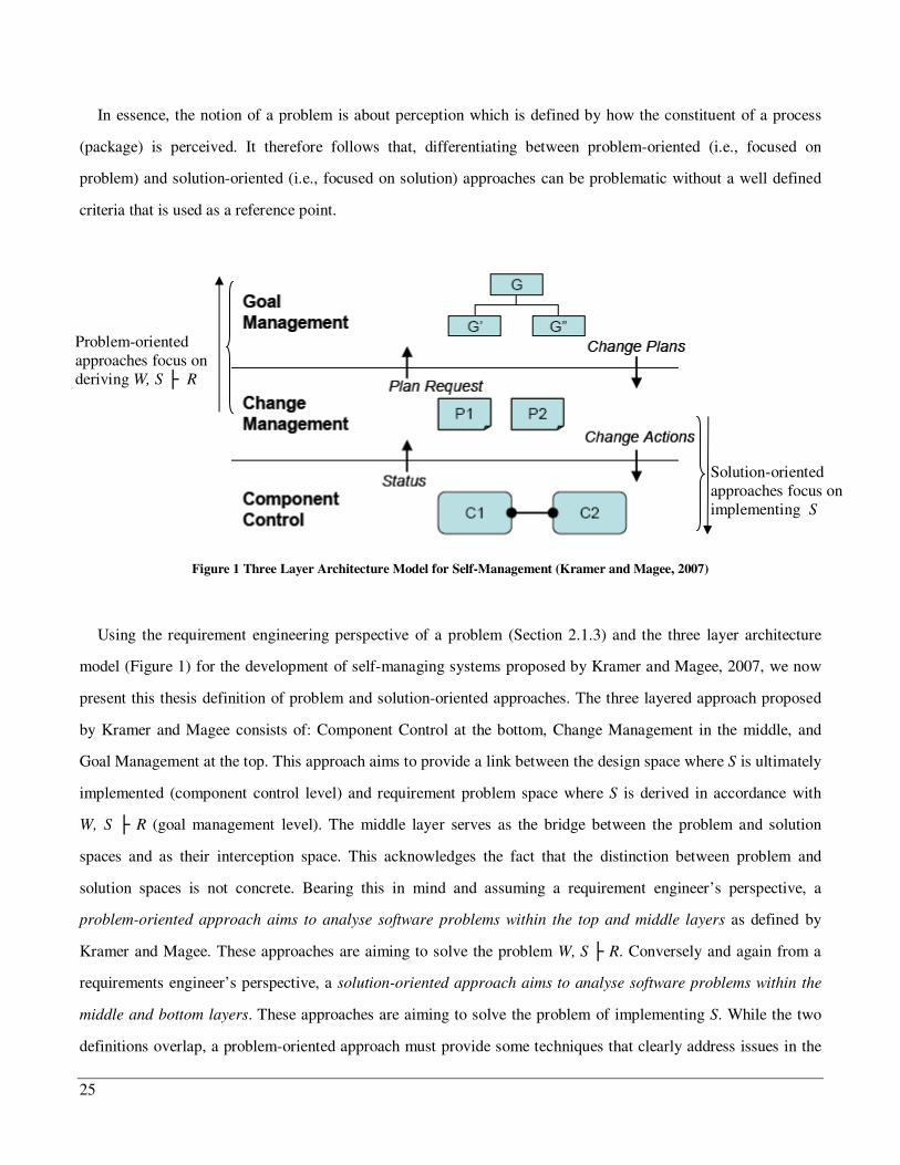
In essence, the notion of a problem is about perception which is defined by how the constituent of a process
(package) is perceived. It therefore follows that, differentiating between problem-oriented (i.e., focused on
problem) and solution-oriented (i.e., focused on solution) approaches can be problematic without a well defined
criteria that is used as a reference point.
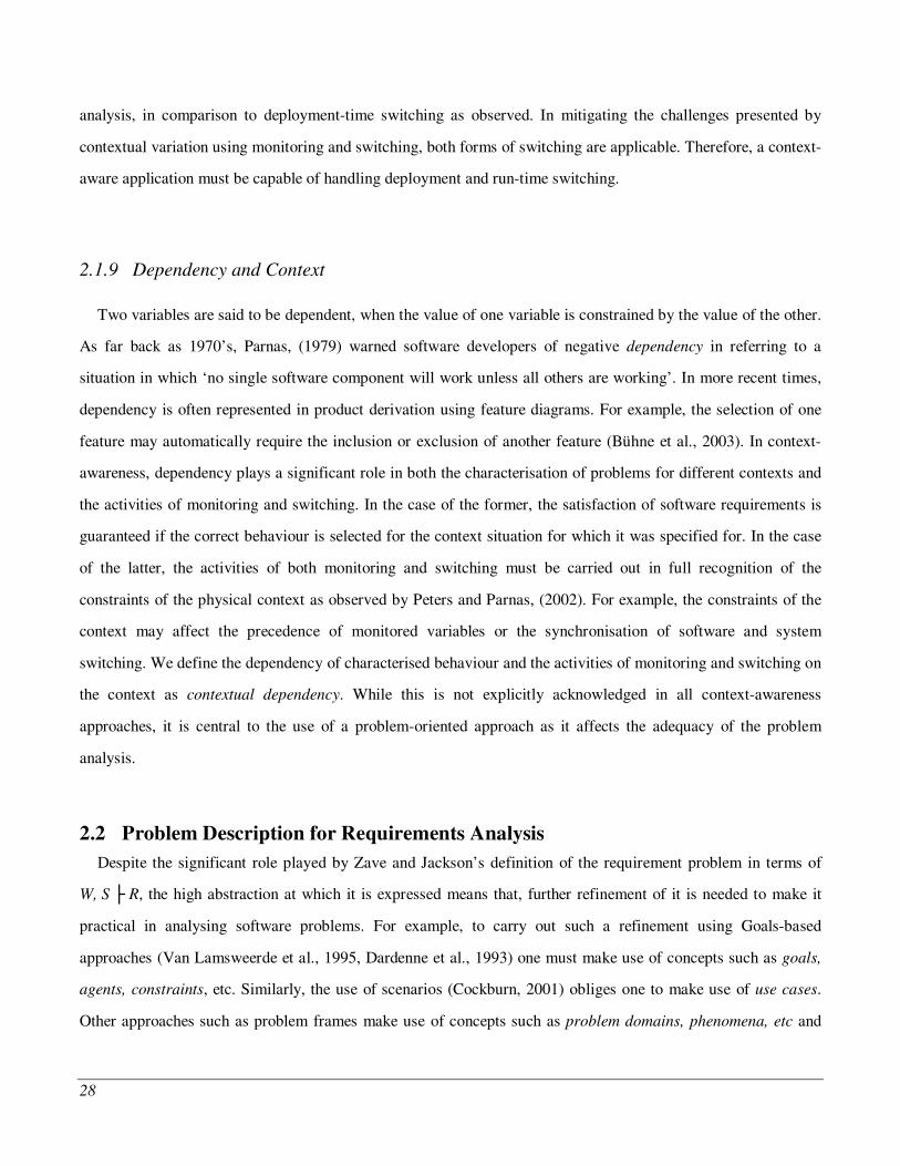
Figure 1 Three Layer Architecture Model for Self-Management (Kramer and Magee, 2007)
Using the requirement engineering perspective of a problem (Section 2.1.3) and the three layer architecture
model (Figure 1) for the development of self-managing systems proposed by Kramer and Magee, 2007, we now
present this thesis definition of problem and solution-oriented approaches. The three layered approach proposed
by Kramer and Magee consists of: Component Control at the bottom, Change Management in the middle, and
Goal Management at the top. This approach aims to provide a link between the design space where S is ultimately
implemented (component control level) and requirement problem space where S is derived in accordance with
W, S R (goal management level). The middle layer serves as the bridge between the problem and solution
spaces and as their interception space. This acknowledges the fact that the distinction between problem and
solution spaces is not concrete. Bearing this in mind and assuming a requirement engineer’s perspective, a
problem-oriented approach aims to analyse software problems within the top and middle layers as defined by
Kramer and Magee. These approaches are aiming to solve the problem W, S R. Conversely and again from a
requirements engineer’s perspective, a solution-oriented approach aims to analyse software problems within the
middle and bottom layers. These approaches are aiming to solve the problem of implementing S. While the two
definitions overlap, a problem-oriented approach must provide some techniques that clearly address issues in the
Problem-oriented approaches focus on deriving W, S R
Solution-oriented approaches focus on implementing S
26
upwards directions (shown on the top left of Figure 1) while solution-oriented approach must have some
techniques for addressing issues in the downwards direction ((shown on the lower right of Figure 1)). Our
definition of a problem-oriented approach is consistent with that of Hall et al, 2007, where the emphasis is on
refinement of W, S R using explicitly formed justifications. The focus of this thesis is on the use of our
problem-oriented approach in analysing the requirements for monitoring and switching activities.
2.1.5 On the Notion of Variability
Variation is an intrinsic property in any software development (van-Gurp et al., 2000). Variation is manifested
in requirements (Faulk, 2001), architecture (Bachmann and Bass, 2001), implementation and even at run-time
(Svahnberg et al., 2005). The notion of variability is often used to describe and analyse the variation in software
applications. In terms of the requirements relation W, S R, variability may occur in all three dimensions
(W, S, and R). While requirements R variation is commonly considered and represents an intrinsic part of the
goal-based requirements approaches (Dardenne et al., 1993, Van Lamsweerde, 2002), specifications S variation is
largely considered in the product-family based approaches aiming for solution reuse in multiple products. There
have been some attempts such as the works of (Liaskos et al., 2006) to consider variations in context W with
limited success which we will elaborate in the follow up Sections in this Chapter. Recall from the research
assumption of this thesis that focuses the attention on variations in W inducing variation in S. Hence, the review of
the related research on variability (in Section 2.3) is based on their ability to analyse variation arising from W.
2.1.6 Software Monitoring and System Monitoring
Monitoring is a recognised technique that is commonly used in both the development (Robinson and
Pawlowski, 1999, Peters and Parnas, 1998) and in the testing and maintenance of software (Fickas and Feather,
1995). Despite this recognition, there is no standard agreed definition for what constitutes the activities of
monitoring. For instance, while some approaches (Mansouri-Samani and Sloman, 1993), focus on the collection
and interpretation of information about ‘objects and software processes’ in the management of distributed
systems, others (Fickas and Feather, 1995) focus on the collection of information about ‘the assumptions made of
the software operating environment and resources needs’ in the assessment of the satisfaction of software
27
requirements. In essence, while the former focuses on the internal state changes of the software, the latter focuses
on the external states changes of the operating environment. In presenting their 4-variable model (inputs/outputs
interfaces to the physical world; and inputs/outputs interfaces to the software) to software description and its
relation to monitoring, Peters and Parnas, 2002, refer to monitoring activities that focus on internal state changes
as software monitors and those focusing on the external environmental states changes as system monitors (Peters
and Parnas, 2002). Of these two, context-awareness requires system monitors as the changes requiring variation in
software behaviour are caused by environmental changes. Therefore, the use of the word monitor or monitoring,
in this thesis, should largely be seen in the context of system monitoring. This view of system is also consistent
with the three descriptions of problems, including those of monitoring, in the problem frames notation.
2.1.7 Software Switching and System Switching
Comparable to software and system monitoring is software and system switching. As in the case of software
monitoring, software switching refers to internal software behavioural adaptations which may involve parameter
adjustment (Feather et al., 1998) or component re-configuration (Georgiadis et al., 2002). System switching refers
to adaptations in the physical environment such as taking an alternative driving route following a request made
through the software. In the case of context-awareness, the difficulty lies in the identification of operating
environments at which software switching such as component reconfiguration is synchronised with system
switching; thereby ensuring that the software adaptations reflects the reality. Therefore, we define switching as
the synchronisation of software and system switching at execution time.
2.1.8 Deployment-Time Switching and Run-Time Switching
Besides system and software switching, another relevant distinction worth considering is that of deployment-
time and run-time (Svahnberg et al., 2005) switching. Deployment-time switching adapts application behaviour
prior to execution and does not interrupt the application while it is being executed. This form of switching is
commonly used in configuration management (Coatta and Neufeld, 1994) but has been explored by Feather et al,
1998, in their approach to reconciling application behaviour during execution. Run-time switching does allow for
the application to be interrupted while it is being executed and thus presents more difficulties in the problem
28
analysis, in comparison to deployment-time switching as observed. In mitigating the challenges presented by
contextual variation using monitoring and switching, both forms of switching are applicable. Therefore, a context-
aware application must be capable of handling deployment and run-time switching.
2.1.9 Dependency and Context
Two variables are said to be dependent, when the value of one variable is constrained by the value of the other.
As far back as 1970’s, Parnas, (1979) warned software developers of negative dependency in referring to a
situation in which ‘no single software component will work unless all others are working’. In more recent times,
dependency is often represented in product derivation using feature diagrams. For example, the selection of one
feature may automatically require the inclusion or exclusion of another feature (Bühne et al., 2003). In context-
awareness, dependency plays a significant role in both the characterisation of problems for different contexts and
the activities of monitoring and switching. In the case of the former, the satisfaction of software requirements is
guaranteed if the correct behaviour is selected for the context situation for which it was specified for. In the case
of the latter, the activities of both monitoring and switching must be carried out in full recognition of the
constraints of the physical context as observed by Peters and Parnas, (2002). For example, the constraints of the
context may affect the precedence of monitored variables or the synchronisation of software and system
switching. We define the dependency of characterised behaviour and the activities of monitoring and switching on
the context as contextual dependency. While this is not explicitly acknowledged in all context-awareness
approaches, it is central to the use of a problem-oriented approach as it affects the adequacy of the problem
analysis.
2.2 Problem Description for Requirements Analysis
Despite the significant role played by Zave and Jackson’s definition of the requirement problem in terms of
W, S R, the high abstraction at which it is expressed means that, further refinement of it is needed to make it
practical in analysing software problems. For example, to carry out such a refinement using Goals-based
approaches (Van Lamsweerde et al., 1995, Dardenne et al., 1993) one must make use of concepts such as goals,
agents, constraints, etc. Similarly, the use of scenarios (Cockburn, 2001) obliges one to make use of use cases.
Other approaches such as problem frames make use of concepts such as problem domains, phenomena, etc and

29
the use of domain theory (Sutcliffe, 1998) requires one to use concepts such as meta-domains, problem domains,
tasks, etc. While all these approaches have concepts for capturing the context of software applications,
distinguishing between physical context and other types of contexts (Sutcliffe, 1998) is not possible in all
approaches. Also, the differentiation between context, specification, and requirements can be difficult in some
approaches. As an example, it has been observed by (Hall et al., 2007) that while goal-based approaches
emphasise the refinement of R, they are rather weak in the refinement of W and S. This is because, the
development of goal-trees is driven by goals and leaf level goals and agents that represent S and W are terminal
which make their refinement implausible. Similar but different limitations are observed in other approaches. To
illustrate this, unlike the goal-based approaches, problem frames approach strongly distinguishes between
W, S, and R. However, while Problem Frames emphasise the refinement of W and S, it is rather weak in the
refinement of R. This is evident in Problem Frames distinguishing between indicative and optative properties in W
thereby, focusing on the refinement of W. While the former captures contextual facts that hold true even in the
absence of S and R, the latter captures the desires of R in W brought about by S. Given that the focus of our
research is on analysing the impact of physical contextual properties W on requirements satisfaction and context-
awareness, we have found the Problem Frames approach to problem description appropriate. It enables us to
capture physical contextual properties and to separate requirements from specifications and context.
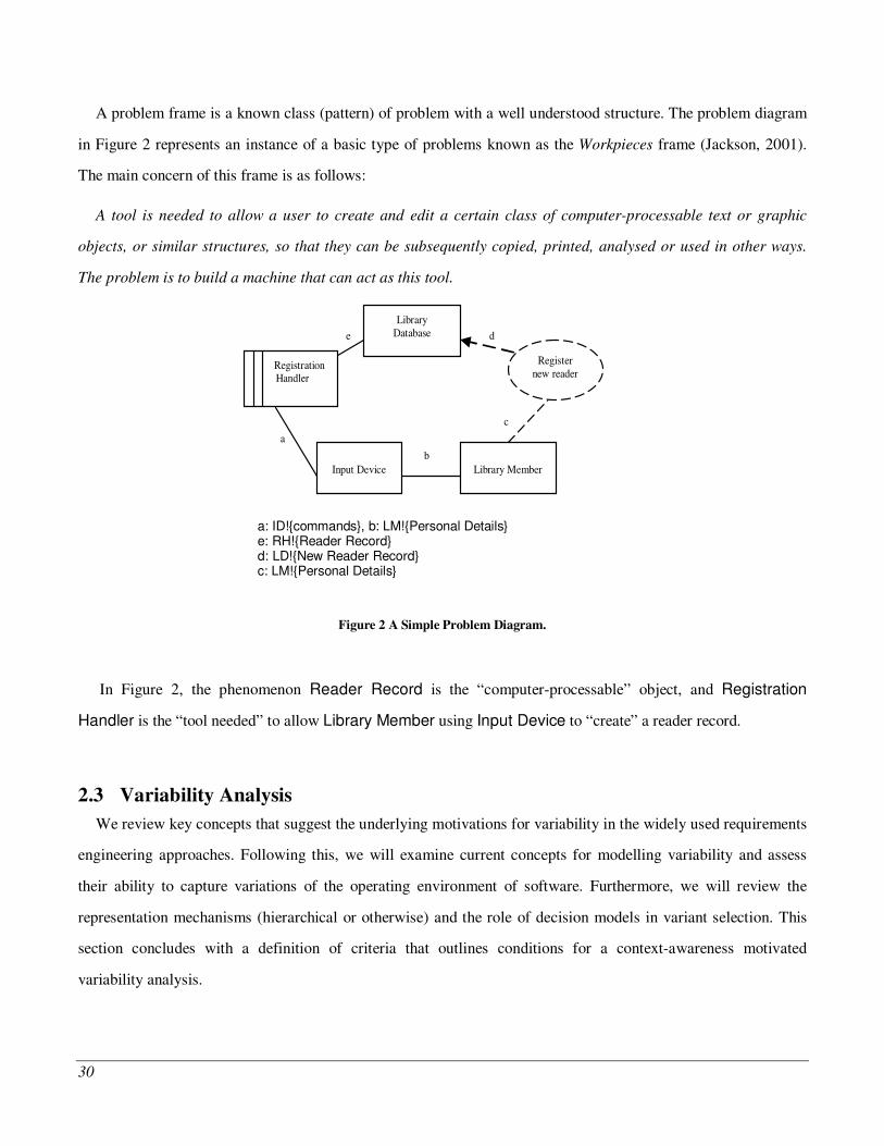
Even though all the approaches reviewed here provide graphical notations for problem descriptions, we only
present that of Problem Frames given that it is the chosen notation for analysing contexts of context-aware
applications in this thesis. This is done with the aid of a simple problem diagram in Figure 2. The rectangles with
no stripes (Library Database, Input Device and Library Member) represent physical domains of the problem
world whose properties are relevant to the problem. The dashed oval represents the requirement, and the rectangle
with a double stripe is the machine domain whose specification is required. Thick lines between the domains
represent sets of shared properties of the domains involved and are referred to as shared phenomena. For example,
the shared phenomenon e indicates that details of reader records are shared between the two domains
Registration Handler (RH) and Library Database (LD). The prefix RH! suggests that RH can manipulate or
control the reader records, whilst LD can only observe them. The dashed line between the requirement and
Library Member (LM) denotes that the requirement references the property of LM, and the dashed line with an
arrow head between the requirement and LD denotes that the requirement constrains the property of LD. It means
that when the library member provides personal details, a new reader record is expected to be added to the Library
Database.
30
A problem frame is a known class (pattern) of problem with a well understood structure. The problem diagram
in Figure 2 represents an instance of a basic type of problems known as the Workpieces frame (Jackson, 2001).
The main concern of this frame is as follows:
A tool is needed to allow a user to create and edit a certain class of computer-processable text or graphic
objects, or similar structures, so that they can be subsequently copied, printed, analysed or used in other ways.
The problem is to build a machine that can act as this tool.
Figure 2 A Simple Problem Diagram.
In Figure 2, the phenomenon Reader Record is the “computer-processable” object, and Registration
Handler is the “tool needed” to allow Library Member using Input Device to “create” a reader record.
2.3 Variability Analysis
We review key concepts that suggest the underlying motivations for variability in the widely used requirements
engineering approaches. Following this, we will examine current concepts for modelling variability and assess
their ability to capture variations of the operating environment of software. Furthermore, we will review the
representation mechanisms (hierarchical or otherwise) and the role of decision models in variant selection. This
section concludes with a definition of criteria that outlines conditions for a context-awareness motivated
variability analysis.
e
d
c
b
Registration Handler
a
Input Device
Register new reader
Library Database
Library Member
a: ID!{commands}, b: LM!{Personal Details} e: RH!{Reader Record} d: LD!{New Reader Record} c: LM!{Personal Details}
31
2.3.1 Eliciting Variability
Despite the ubiquity of variability in system development, its treatment in analysing software applications is
not always explicit. For example, Jackson, (2001) uses the notion of frame flavour and variant frames to
implicitly capture variations in W in the W, S R relation. Implicit in the sense that, both frame flavours and
variant frames were meant for analysing systems with differing contexts at different times, not at the same time as
necessary in the case of context-aware systems. Frame flavours are used to capture variations at a lower level of
abstraction, focusing on issues such as differences in data structures. On the other hand, variant frames are used to
capture variations at a much higher abstraction, focusing on issues of variation in control and in problem domains.
In contrast to the implicit treatment of variability in problem-frames, the product-family approaches based
paradigm (Bosch et al., 2002, Bosch, 2000, Sinnema et al., 2006, Jaring et al., 2004, Sochos et al., 2004, Parnas,
1976) have overwhelmingly considered variability as the central issue in developing families of software. To
understand the disparity in the treatment of variability, we need to examine, critically, the underlying motivations
for analysing variability.
Even though the notion of software product-family became popular in the mid-1990s culminating in the
establishment of the Software Product-Line Conference (SPLC) series1, the idea has long been championed as far
back as the 1970s (Parnas, 1979, Parnas, 1976). The underlying motivation then and now is reuse in an identified
group of software aiming to satisfy different market segments (Moorthy, 1984, Dickson and Ginter, 1987,
Claycamp and Massy, 1968). This is acknowledged to contribute to the reduction in both the cost and
management effort (Northrop, 2002, Ommering, 2002). Parnas argued that if one was to develop a group of
related software over a given time period, then one could save cost and effort by explicitly analysing the
commonality in all the software upfront. Following this, one will be in a position to determine the sequence of
refinements needed to cope with the additional individual functionality inducing the variability among the
product-family. However, in order to analyse a group of related software for both present and future use, a
detailed understanding of the application domain2 is needed. Therefore, domain analysis (Fowler, 1997, Sutcliffe,
1998, Frakes et al., 1998) is seen as a fundamental part in analysing a product-family aiming to identify both the
commonality and variability. Contrasting the product-family’s motivation with that of context-awareness which is
focused on the classification of problems for different contexts, although reuse may be possible in the
1 http://www.splc.net/
2 Application domain as used here is analogous to meta-domains as defined by Sutcliffe, 1998. E.g., telecommunication and banking sectors.
32
characterised problems, it is not the overriding objective as the presence of related group of software is not a pre-
requisite in the analysis of context-awareness.
Unlike product-family, the motivation for variability analysis in goal-based approaches (Dardenne et al., 1993,
Castro et al., 2002, Yu, 1997, Hui et al., 2003), until recently (Liaskos et al., 2006), has been on refining
stakeholder intentions. In other words, abstract stakeholder goals are refined to concrete ones assignable to agents
that ensure their satisfaction. It has long been the accepted wisdom that stakeholders often cannot give sufficient
clear description of their goals or likely to change their mind given new developments (Nuseibeh, 2001, Van
Lamsweerde, 2002). Therefore, it falls on the requirement engineer to investigate alternative ways of achieving
the more abstract goal during the refinement process, in the hope that changes made by the stakeholder, during the
development process, will be accommodated. Hence, the underlying motivation in this case is the adequacy of the
refinement in uncovering all relevant alternatives ways of satisfying the abstract goals. Knowledge about shared
intentions captured in non-leaf (abstract) goals have been used as the basis for selecting alternative behaviours in
the event of leaf-goals failures (Lapouchnian et al., 2006). Again, contrasting the motivation of refining the
stakeholder’s intentions with that of context-awareness, while the refinement of intentions is certainly relevant in
the characterisation of problems for different contexts when there are observed dependency between stakeholders’
intentions and contexts, the motivations for problem classification may be unintentional (Liaskos et al., 2007). It
is the latter form of context-awareness that we choose to focus on in this thesis.
The motivation behind the use of frame flavours and variant frames by Jackson is problem matching. By this
we mean, the matching of a given problem at hand to a known problem class such as the commanded behaviour
frame (Jackson, 2001). This motivation is shared by other approaches such as domain theory (Sutcliffe, 1998) and
pattern-oriented approaches (Rajasree et al., 2003, Chandra and Bhattaram, 2003, Fowler, 1997, Hallsteinsen et
al., 2004, Meister et al., 2004, Keepence and Mannion, 1999). Unlike the product-family paradigm where a group
of related software must be analysed together upfront in the quest for commonality and variability, problem
frames and pattern-oriented approaches do not require the presence of such a group. Instead, they are focused on
providing a starting base for analysing similar problems aiming to facilitate knowledge reuse. Hence, the
emphasis is on the commonality in the problem rather than the variability. Again, the motivation of problem
matching is relevant to that of context-awareness, especially where the underlying causes of behavioural
variations are unintentional, in the characterisation of problems. This may take the form of using a problem class
when it can be tailored to a given context. Alternatively, given that several problems are needed for different
33
contexts, an already characterised problem which may not be based on a known problem class could still be
tailored and used in a different context. Hence, while the use of problem frames is useful in problem
classification, their availability is not a prerequisite in analysing context-aware applications.
Another commonly used software development approach is use cases (Cockburn, 2001). Use cases are often
used to capture the usage scenarios (Sutcliffe et al., 1998) of the software-to-be. The underlying motivation for
use cases is the refinement of scenarios so as to consider possible extensions to the ‘normal’ usage of the
software. While use cases capture the details of the sequence of activities encountered when the software is used,
they are rather limited in their ability to capture details of the physical context surrounding the activities.
Nevertheless, scenarios have been used in analysing the requirements for context-aware applications (Sutcliffe et
al., 1998, Sutcliffe et al., 2005). Given their limitations in capturing the physical context, it is our view that they
are insufficient in analysing context-awareness where the motivations for problem classification are unintentional
and contextual.
2.3.2 Modelling Variability and Selecting Variants
Having reviewed some key motivations for the implicit or explicit analysis of variability, we now take a
detailed look at how these differing motivations influence the modelling of variability. Variability modelling
refers to the visual display of variants highlighting their dependency. The subject of reuse comes from multitude
of sources including knowledge, intention and solution. For example, (Bachmann and Bass, 2001) have identified
six sources of software variability. These are variations in function or features, such a word-processor with a
voice-recognition system (high-end) or one without (low-end); variation in the data used by components for
communication, such as using a stack or queue, a variation in control flow such as two components
communicating using a publish-subscribe communication pattern (Rozanski and Woods, 2005) or a dedicated
communication channel. Other sources of variability are variations in technology, variations in quality
requirements (Chung et al., 2000) and variations in the target operating platforms.
Motivated by the need to reuse solutions in a related group of software, variability is modelled using the notion
of variation points represented in a feature tree (Metzger et al., 2007, Schobbens et al., 2006). A variation point
represents a non-leaf level node where alternatives are represented for selection. Therefore, a variation point
consists of more than one alternative. A feature as used in the product-family represents a solution to a piece of
34
software functionality. Variants available at variation points have been largely classified into three main types
(Bachmann and Bass, 2001, Svahnberg et al., 2005, Mannion et al., 2000): optional, single and multiple variants.
An optional variant is included in some product members but not in others, for instance including a camera in a
mobile phone. In the case of single variant, exactly one variant is chosen from a candidate set and all others
discarded. In the case of multiple variants, more than one variant must be selected from a candidate list, for
example dual communication protocols for a mobile phone, thereby giving it a wider area of operational access.
There are various combinations of these basic types reported in (Bachmann and Bass, 2001). This rigid
classification is unsatisfactory in the presence of contextual changes as functionalities in a given set and for a
single device may be classified as single variant (i.e. mutually exclusive) in one context and multiple variant (i.e.
to be selected together) in another context. Also, while feature diagrams enable one to view and to analyse several
features together at the same time, in term of the three-category-classification, they are rather weak at providing
details of the underlying problems, which the feature solution fragment represent. This is largely due to the
practical limitations of showing detailed information in the nodes of (graphical) feature-trees which are
hierarchically structured. This has led to approaches (Classen et al., 2007, Bühne et al., 2003, Bachmann and
Bass, 2001) aiming to complement feature-models with detailed problem descriptions thereby enabling one to
have both the detailed problem description and higher abstraction, which are represented in feature-models. The
proposed use of augmented feature diagrams is analogous to the use of Work Breakdown Structures (i.e., feature
models) and Work Breakdown Structures Dictionary (i.e., Detailed Problem Description) (PMI, 2004). In
essence, feature models define the scope from which individual products are derived. However, the derivation of
individual products requires some form of selection criteria that clearly defines the conditions for doing so. The
collection of criteria relevant to a feature model is captured in decision models. Decision models may be rule-
based (Buchanan, 1984, McDermott, 1980), policy-based (Badr et al., 2004), task-based (Cousin and Collofello,
1992) or constraints-based (Borning and Duisberg, 1986). The application of decision models in individual
product derivation may be supported by tools. The use of a decision model to select a variant at a variation point
(i.e., variation point binding), may be done at design time prior to the loading of the software onto hardware
devices such as mobile phones (Maccari and Heie, 2005), or at run-time as commonly used in the customisation
of desktop applications (Poladian et al., 2004), or even during the operation of the software as used in dynamic
reconfigurable systems (Georgiadis et al., 2002). Svahnberg et al, 2005 have done a detailed review of variability
realisation techniques across the software development process. Similar to the derivation of individual products
for different market-segments using decision models, context-aware applications must derive behaviours for
35
different contexts which also require the use of decision models. However, while detailed problem descriptions
are needed in the characterisation of problems for different contexts for context-awareness analysis, a hierarchical
display of the characterised problems as in feature models is not a prerequisite. This is because the solutions of
the characterised problems may ultimately be loaded into a single device as opposed to multiple devices as
practiced in product-family.
In the case of Goal-based Modelling, where higher (more abstract) goals are recursively refined until lower
(more concrete) goals are obtained, the concept of OR-decomposition is used to capture variability in goals
(Dardenne et al., 1993, Van Lamsweerde, 2002). Recall that the motivation for this form of refinement is the
clarification of user requirements and the identification of alternatives aiming to provide the stakeholder adequate
information to make a choice they otherwise might not be able to do so using the more abstract goal. In striving
for adequacy , some goal-based approaches such as KAOS (Dardenne et al., 1993) turn to formalism that enable
them to define and verify some notion of completeness. Other approaches such as Yu, 1997 (I*), turn to factors
such as variation in the quality requirements (Chung et al., 2000) as the basis for eliciting alternative goals in OR-
decompositions. In recent times, others (Liaskos et al., 2006, Liaskos et al., 2007) have broaden the factors to
include environmental properties such as variation in location and time which they define as background
variability. They argued that feature diagrams do not take background variability into consideration and are
therefore unsuitable for representing and reasoning about variability of systems where environmental changes are
common place. As we argued in the preceding sections, the limitation of feature models is not about the type of
information they represent but more to do with the depth at which information is represented. This fact is
illustrated in using feature models to capture both functional and operating platform variability (Svahnberg et al.,
2005, van-Gurp et al., 2000). Irrespective of the underlying cause of the variability, as in the case of feature
models, a decision must be made at some stage in the software development process as to which alternative to
take. In goal-based approaches, the notion of rationale (Chung et al., 2000) and preference model (Liaskos et al.,
2006) have been used for variant selection. Also as in the case of product-family, decision models are needed for
selecting alternatives irrespective of whether the motivation is intentional or unintentional in context-aware
applications. However, the focus of goal-based approaches on refining stakeholder intentions (less on context and
specification) and despite the explicit consideration of unintentional sources in refining goals (Liaskos et al.,
2006), the limitations of goals in the refinements of context (Hall et al., 2007) makes it difficult to use in
analysing the problems of context-awareness.

36
Problem frames is broadly considered a type of pattern oriented software development approach (Rajasree et
al., 2003). Variability modelling and variant selection have not been considered in the problem frames approach
and the pattern-oriented software development as a whole, in the sense of problem classification for context-
awareness. This is not surprising considering that the underlying motivation is problem matching in support of
knowledge reuse. In essence, the primary focus has always been on the tailoring of the problem class generic
structure to a given problem at hand. In doing so, the focus has always been on detailed problem description of
the given (single) problem and not about how variations in different problems considered together (Parnas, 1976)
are represented. It therefore follows that, since there is only one problem at hand, there is no role for decision
models in this case. Instead, what is needed is some form of guidance (i.e., heuristics) in tailoring the generic
problem structure to fit the individual case at hand. In problem frames, Jackson’s proposed use of the frame
flavours and variant frame (Jackson, 2001) aim to provide such a guidance. Similarly, Sutcliffe proposed the use
of catalogues in analysing his proposed classes of problems (Sutcliffe, 1998). While the level of details captured
in problem classes makes them suitable for problem classifications, the implicit assumption of a single problem
analysis means that, such an approach must be adapted when used to analyse context-awareness problems as
multiple problems are being considered for different contexts which requires the use of decision models at run-
time. The approach presented in this thesis makes such an adaptation to enable the use of problem frames in the
analysis of context-aware applications.
In summary, following the detailed review of the concepts outlining the underlying motivations and modelling
of variability in the various software development approaches, we can now summarise their strengths and
limitations as shown in Table 1 and Table 2.
Approach Key
Motivations Modelling Concept
Representation Context
Description Variability
Type Variant
Selection
Features Configuration of
Multiple Products.
Variation Point Hierarchical Low
Intentional, Unintentional,
Explicit
Decision Models
Goals Intention
Refinement OR-Goal
Decomposition Hierarchical Medium
Intentional, Explicit
Rationale
Problem Patterns
Matching to known problems
Problem Customisation Non-Hierarchical High
Unintentional, Implicit Heuristics
Use Cases Scenario
refinement Use Case
Extensions Hierarchical Medium
Intentional, Unintentional,
Explicit
Decision Models
Table 1: Comparison Matrix for Variability Analysis Mechanisms in Requirements Engineering
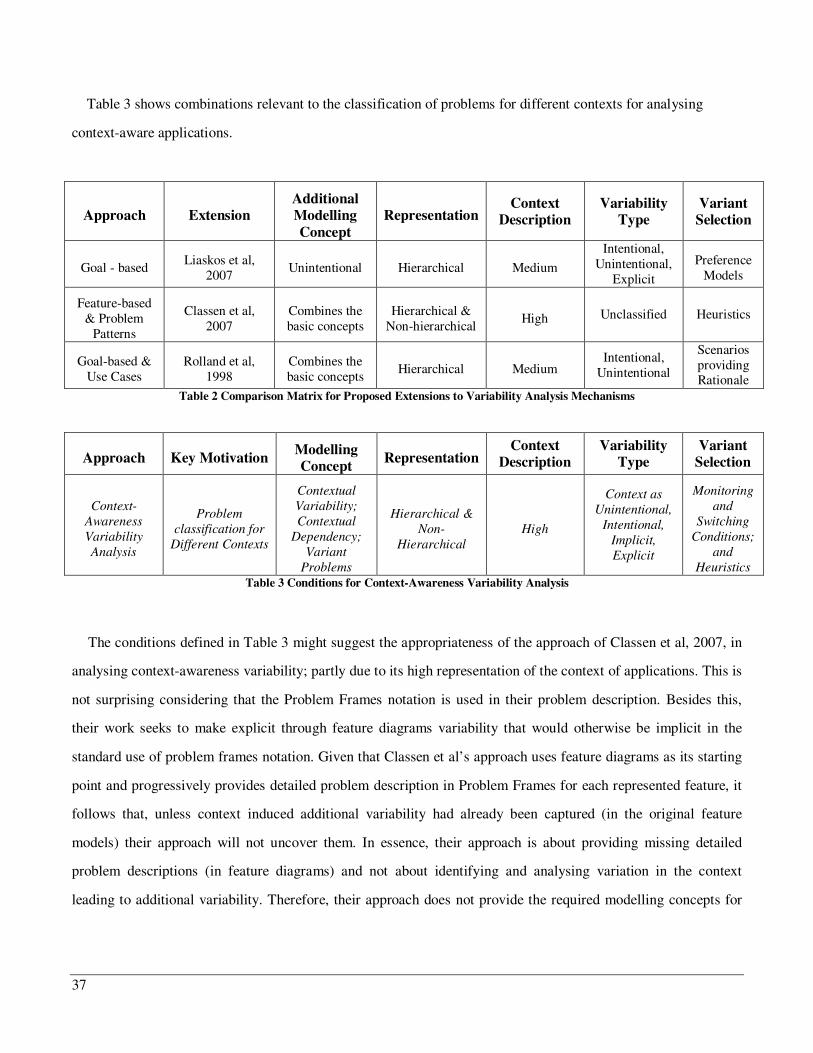
37
Table 3 shows combinations relevant to the classification of problems for different contexts for analysing
context-aware applications.
Approach Extension Additional Modelling Concept
Representation Context
Description Variability
Type Variant Selection
Goal - based Liaskos et al,
2007 Unintentional Hierarchical Medium
Intentional, Unintentional,
Explicit
Preference Models
Feature-based & Problem
Patterns
Classen et al, 2007
Combines the basic concepts
Hierarchical & Non-hierarchical
High Unclassified Heuristics
Goal-based & Use Cases
Rolland et al, 1998
Combines the basic concepts
Hierarchical Medium Intentional,
Unintentional
Scenarios providing Rationale
Table 2 Comparison Matrix for Proposed Extensions to Variability Analysis Mechanisms
Approach Key Motivation Modelling Concept
Representation Context
Description Variability
Type Variant
Selection
Context-Awareness Variability Analysis
Problem classification for
Different Contexts
Contextual Variability; Contextual
Dependency; Variant
Problems
Hierarchical & Non-
Hierarchical High
Context as Unintentional,
Intentional, Implicit, Explicit
Monitoring and
Switching Conditions;
and Heuristics
Table 3 Conditions for Context-Awareness Variability Analysis
The conditions defined in Table 3 might suggest the appropriateness of the approach of Classen et al, 2007, in
analysing context-awareness variability; partly due to its high representation of the context of applications. This is
not surprising considering that the Problem Frames notation is used in their problem description. Besides this,
their work seeks to make explicit through feature diagrams variability that would otherwise be implicit in the
standard use of problem frames notation. Given that Classen et al’s approach uses feature diagrams as its starting
point and progressively provides detailed problem description in Problem Frames for each represented feature, it
follows that, unless context induced additional variability had already been captured (in the original feature
models) their approach will not uncover them. In essence, their approach is about providing missing detailed
problem descriptions (in feature diagrams) and not about identifying and analysing variation in the context
leading to additional variability. Therefore, their approach does not provide the required modelling concepts for
38
analysing contextual variation. In Chapter 3, we present our approach for classifying problems for different
context aiming to satisfy all but one of the conditions identify in the bottom row of Table 3.
2.4 Monitoring and Switching Requirements
We review current approaches to monitoring and switching activities focusing on their overall Concepts
outlining their underlying objectives. By underlying objectives we mean, the dominant motivations as highlighted
in the related publications. Given the numerous publications on monitoring and to a lesser extent on switching, we
have classified the works into five categories: checking for requirements inconsistency, execution failure
diagnostics, software compliance testing, performance tuning, ubiquitous computing, and self-managing. Where
necessary, the work is further discussion in terms of development-time and run-time approaches. We acknowledge
that these categories do not represent disjoint groups and that most of them might cover more than one of these
categories. Nevertheless, we find this categorisation useful in reviewing the strengths and limitations of the works
in relation to the problems outlined in this thesis. In this regard, we assess the ability of the approaches to capture
external contextual properties and to analyse the impact of such properties on monitoring and switching. Also
asses are their ability to analyse contextual dependency and requirements trade-off and their impact on monitoring
and switching respectively. This section concludes with the definition of a criterion for a problem-oriented
approach for analysing monitoring and switching problems.
2.4.1 Requirements Inconsistency
Monitoring has been found to be useful in the discovery and analysis of inconsistency in software development
(Robinson and Pawlowski, 1999, Peters, 2000). Enabling software developers to set development requirements
goals, the approach developed by Robions and Pawlowski provides the mechanism for detecting inconsistencies
arising due to variances in what is produced by developers and what was expected. In essence, it is the
development goals that are monitored and not the original stakeholder goals. This is based on the assumption that
inconsistency in the development goals will lead to problems in the satisfaction of the original stakeholder goals.
Similarly to the approach taken by Robinson and Pawlowski, the approach taken by Peters provides a mechanism
for checking derived specifications for the existence or absence of prior defined properties. Again, this approach
does not check the specifications for the satisfaction of the original stakeholder goals and requirements; instead, it
39
focuses on checking the quality of the derived specifications from which it infers the possible state of the original
stakeholder requirements. While these two approaches may be relevant for the analysis of context-awareness, it is
more paramount to be able to discover inconsistency at run-time and in those arising in the stakeholder
requirements itself. Furthermore, their prior detection and analysis during problem classification is what is crucial.
Also, given the focus of these approaches on the development-time, the activities of switching are not considered.
Instead, the focus is on the presentation of the detected inconsistency to the developers who will subsequently
take corrective actions to ensure the ultimate satisfaction of the stakeholders’ requirements. Given that context-
aware applications must rely on themselves for behaviour adaptation, the activities of switching are fundamental
in their analysis.
2.4.2 Failure Diagnostics
Current monitoring approaches (Robinson, 2002, Robinson, 2005, Wang; et al., 2007, Winbladh et al., 2006)
on requirements failure diagnostics focus on execution failures. While the use of the ReqMon approach
(Robinson, 2002, Robinson, 2005) makes no assumption of points of failure and therefore claims to exhaustively
investigate all failure sources, the approach taken by Wang et al identifies and defines possible failure points
thereby restricting their diagnostic analysis space at run-time. The primary distinction between the approaches of
Wang et al and Winbladh et al is that, while the former allows for variation in the abstraction level of monitored
event, depending on the level on a goal-tree, the latter assumed a fixed abstraction level that might make it
inefficient in some contexts. What all these approaches have in common is their focus on the execution failure as
the triggering event for diagnostics. This is insufficient in the case of context-awareness (Feather et al., 1998,
Fickas and Feather, 1995). This is because, although the software execution may be successful, if it takes place in
an environment in which the assumptions made of it are invalid, the requirements will not be satisfied. Also, the
absence of automated switching activities in Wang et al’s and Windbladh et al’s approaches make them
incomplete in the analysis of the entire scope of context-awareness. Even though the approach taken by Robinson
does provide some automated switching activities, the approach is still limited by both the reliance of only
internal system execution states and software switching without assessing the impact of such activities on the
external operating environment (e.g., system switching).
40
2.4.3 Testing and Maintenance
Monitoring approaches on software requirements compliance testing (Feather et al., 1998, Fickas and Feather,
1995, Cohen et al., 1997, Peters and Parnas, 2002, Robinson, 2006) do consider both internal and external
environmental factors. For example, while some approaches focus on monitoring changes in the assumptions
made of the physical environment and its impact on continual requirements satisfaction (Feather et al., 1998,
Fickas and Feather, 1995), others focus on the reliability of the interfacing between the software and the physical
world and its impact on monitoring activities (Peters and Parnas, 2002). While we acknowledge the relevance of
the latter in the analysis of context-aware applications, it is the former that is considered most relevant to the
approach taken in this thesis given its closeness to the requirement analysis space. However, while Feather et al
consider the activities of monitoring in the problem-space, the activities of switching is deferred till the solution
space. Therefore, the analysis of possible constraints in the synchronisation of software and system switching is
missing. This is crucial for context-aware applications due to the need to explicitly consider the environment in
assessing their requirements satisfaction. Robinson proposed an approach that builds on the one taken by Feather
et al, 1998 (Robinson, 2006). The proposed approach focuses on the testing of enterprise software in distributed
service-oriented (Harrison, 2005) environment. Given the dependency of Robinson’s approach on the Feather et
al’s, the limitations observed in Feather et al’s approach are inherited as well.
2.4.4 Performance Tuning
Software quality requirements (Chung et al., 2000) such as performance and usability are used to assess how
well software is meeting its functional requirements. Quality requirements may be the subject of monitoring and
switching activities. For example, there are several approaches (Hofmann et al., 1994, Haban and Wybranietz,
1990, Mansouri-Samani and Sloman, 1993) that focus on software performance tuning, aiming to determine how
well the software is meeting its requirements. While they may assess the satisfaction of the requirements as in the
case of diagnostics and testing, they are primarily focused on the efficiency of the software. Where the computing
resources being used is the subject of the performance assessment (Mansouri-Samani and Sloman, 1993), then the
overhead of the monitoring activities is a primary concern and must be analysed. While such an overhead may be
relevant in context-awareness when its affect the satisfaction of the requirements, the primary focus is on the
41
satisfaction of the original stakeholder requirements underlying the fact that efficiency may be compromised in
ensuring their overall satisfaction.
2.4.5 Ubiquitous Computing
Prior to the renew focus of research activities on self-managing (Kramer and Magee, 2007), research into the
development of context-aware software was largely driven by the ubiquitous computing research community
(Abowd, 1999, Abowd and Mynatt, 2000, Kindberg and Fox, 2002, Grimm et al., 2001, Harter et al., 2002). It is
worth noting that the scope of problem analysis require by ubiquitous computing is broader than what is required
for context-aware applications. For example, a critical look at the discussion of Abowd and Mynatt reveals at least
three problem areas: the analysis of the human-computer interaction interface (HCI); the analysis of context-
awareness (as defined in this thesis); and the recording of live events for lessons learned or replays. Therefore,
the role of context-aware techniques aiming to achieve self-managed status were employed to meet the non-
intrusiveness challenge (Weiser, 1993a, Weiser, 1993b). Also, most of the focus of these approaches were either
skewed towards the HCI part of the problem (Salvador et al., 2004) or towards the development of middleware
infrastructure for the implementation of context-aware application (Grimm et al., 2004, Kindberg and Fox, 2002).
Given the focus of these approaches, problem classification for different contexts and the analysis of the impact of
context on monitoring and switching activities are missing. In essence, the systematic separation of concerns in
the analysis of context-aware problems is absent.
2.4.6 Self-Managing
Current research into self-managing applications, which is also known as autonomic computing (Kramer and
Magee, 2007), is predominantly focused on the architecture for such systems (Kephart and Chess, 2003,
McKinley et al., 2004b, Kramer and Magee, 2007). However, there are exceptions such as the work of
Lapouchnian et al, 2006 which proposed the use of a goal-based approach to analyse the requirements for
autonomic application. Also, there have been attempts (Gomaa and Hussein, 2004a, Gomaa and Hussein, 2004b,
Apel and Böhm, 2005, Kim et al., 2005) at using variability in the design of reconfigurable architectures, each of
which will be discussed next. The configuration of an architecture refers to its set of components, their
42
interconnections and the constraints defining the behaviour of this architecture (van der Hoek, 1999). The
replacement of such a configuration with a new (or different) one after it has been released or during the operation
of the applications based on it, is referred to as reconfiguration (Oreizy et al., 1999, Kramer and Magee, 1990).
Architectural styles or patterns (Abowd et al., 1993), such as the client-server architectural style, have been used
to construct reconfiguration patterns that are based on the styles of the generic architectures (Gomaa and Hussein,
2004a, Gomaa and Hussein, 2004b). A reconfiguration pattern is used to guide the process of automatically
deriving one architectural configuration from a different one. This can be argued to be a generalised form of
parameterisation (Perry, 1998) as all instances of this product-family must conform to the style and different
members are instantiated by changing the values of parameters. The focus of Gomaa and Hussein is on managing
transitions from one configuration to another during reconfiguration, which is assumed to take place at
deployment-time. Hence, there is no explicit discussion of the impact of dynamically changing the operating
context on defining and reasoning about problem classification, monitoring and switching activities. The
assumption that architecture reconfiguration takes place at deployment-time, which implies that applications do
not undergo any dynamic adaptation of their structure during operation makes this unsuitable for “truly” context-
aware applications. The work of Kim et al, 2005 is similar to that of Gomaa and Hussein, hence exhibits the same
limitations. The key difference is that Kim et al. provide an architectural description language for describing
architectures and modifications to be applied to them during reconfiguration. Again, as with Gomaa and Hussein,
the focus of this approach is on managing the transition from one configuration to another during reconfiguration.
Also, the assumption that architecture reconfiguration takes place at application launch by this approach appears
to make it unsuitable for context-aware applications.
In summary, the focus of the approaches reviewed in this section is on reconfiguration at deployment, which
results in the difficult problems of switching application behaviour during execution and that of physical context
monitoring remaining unaddressed. Where dynamic reconfiguration is considered (Apel and Böhm, 2005, Want et
al., 1995, Poladian et al., 2004, Grimm et al., 2004, Kramer and Magee, 2007), a detailed analysis of the contexts
of applications and its relation to problem classification and the activities of monitoring and switching are
missing.
2.4.7 Other Works
Unlike the approaches reviewed thus far, other approaches (Zhang and Cheng, 2006b, Zhang and Cheng,
2006a) have focused their research on the activities of switching. These are primarily focused on the collaboration
43
of multiple threads during software execution which make them amenable to analysing self-managing
implementation related issues (Brown et al., 2006, Janik and Zielinski, 2006, Magee and Maibaum, 2006, Cheng
et al., 2006). Zhang and Cheng have proposed general switching semantics without giving details on how such
semantics relate to physical contextual changes. In an attempt to address this limitation, others (Brown et al.,
2006) proposed augmenting Zhang and Cheng’s approach with goal-based models, that capture the higher level
requirements of the underlying switching semantics. However, while goals are suitable for the capture and
refinement of R, they are not intended for the analysis of W and S (Hall et al., 2007). The detailed analysis of the
problem context (W) is imperative in specifying the behaviour of context-aware applications.
In summary, having reviewed concepts outlining the motivations for monitoring and switching in current
approaches, we can conclude that what all these approaches have in common is the lack of detail analysis of
application environment and the constraints it places on the characterisation of problems and the activities of
monitoring and switching. These are the issues addressed in this thesis.
2.5 Automated Analysis Support
The role of tool support in the analysis of software requirements in general is recognised to be imperative for
the adoption of new techniques and approaches due to the overhead of carrying out detailed problem analysis
(Cheng and Atlee, 2007, Nuseibeh and Easterbrook, 2000). This applies to the analysis of self-managing
applications which is relevant to context-aware applications (Kramer and Magee, 2007). We review the use of
tools in variability analysis and that of monitoring and switching activities next.
2.5.1 Support for Variability Analysis
The role of tools in the analysis of variability can largely be categorised into two categories: support for
variant elicitation and analysis on one hand and variant selection on the other. In the case of the former, Liaskos
et al, 2006, suggest the use of linguistics theory (Fillmore, 1967) to analyse stakeholder requirements which
formalises variability sources and makes them amenable to tool supported analysis. While this may be useful in
analysing variations arising in R, it will be problematic in the analysis of those arising from W as stakeholders are
not always in the position to express the operating environment of software applications. The use of tool support
44
in variant selection during individual product derivation in product-family development (Metzger et al., 2007) or
in the reconfiguration of application in configuration management (van der Hoek, 1999) is widely researched. In
the case of Metzger et al, the problem of variant selection is first transformed into constraint satisfiability
formulae which they solve using an off-the-shelf standard SAT-Solver. Given the fact that the derivation is done
offline, the overhead of using the SAT-Solver does not affect the subsequent performance of the derived
individual product. In the case of Hoek, to support the dynamic reconfiguration of application behaviour at runt-
time, policy-based decision models are pre-computed at design time. Hoek’s approach is analogous to the use
preference models generally (Liaskos et al., 2006). However, unlike Hoek, Liaskos et al used situation calculus
(Pinto, 1993) in formulating their preference models and not policies. The use of decision models is relevant to
context-aware applications in two folds: primarily in the selection of characterised behaviours for different
contexts during application execution; and in the control of monitoring activities such as the initialisation and
termination of individual monitors in different contexts. The limitation of decision models (Liaskos et al., 2006,
van der Hoek, 1999, Metzger et al., 2007) is the absence of detailed analysis of the application context and
explicit consideration of the constraints of the context in the derivation of the decision models.
2.5.2 Support for Monitoring and Switching Analysis
The use of tools in the analysis of monitoring can largely be grouped into two categories: those focused at
deriving the requirements for monitoring from stakeholder requirements (Peters and Parnas, 1998, Feather et al.,
1998, Wang et al., 2007, Winbladh et al., 2006) and those focused on the automatic generation of monitoring
activities implementation code (Robinson, 2002). Approaches that focus on the former require the formalisation
of the stakeholder requirements in order to make the automatic derivation of monitoring requirements possible.
Also, while such approaches generally assume a fixed abstraction level that must always be monitored, the
approach taken by Wang et al allows for variation in abstraction. Similarly to the use of SAT-Solvers in (Metzger
et al., 2007) but focusing on monitoring and not product derivation, Wang et al, have used SAT-Solvers for the
automated analysis of monitoring activities of internal system state for fault detection and diagnostics. However,
this is limited by its inability to detect requirements violations caused by contextual changes. Also, switching is
not addressed in their approach. In the case of the use of tool in the automatic generation of monitoring code
(Robinson, 2002), the generated code is not merged with the original program code but runs along side it. Given
that current effort at analysing switching activities is focused in the implementation, tool support for this is largely
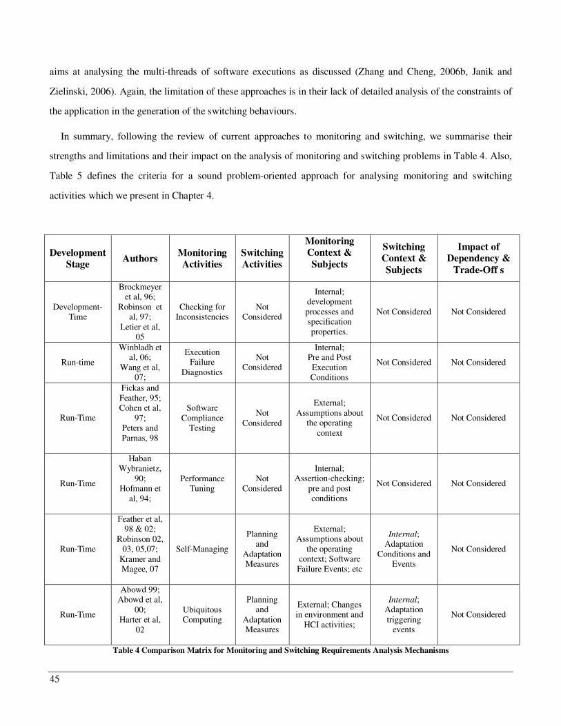
45
aims at analysing the multi-threads of software executions as discussed (Zhang and Cheng, 2006b, Janik and
Zielinski, 2006). Again, the limitation of these approaches is in their lack of detailed analysis of the constraints of
the application in the generation of the switching behaviours.
In summary, following the review of current approaches to monitoring and switching, we summarise their
strengths and limitations and their impact on the analysis of monitoring and switching problems in Table 4. Also,
Table 5 defines the criteria for a sound problem-oriented approach for analysing monitoring and switching
activities which we present in Chapter 4.
Development Stage
Authors Monitoring Activities
Switching Activities
Monitoring Context & Subjects
Switching Context & Subjects
Impact of Dependency &
Trade-Off s
Development-Time
Brockmeyer et al, 96;
Robinson et al, 97;
Letier et al, 05
Checking for Inconsistencies
Not Considered
Internal; development processes and specification properties.
Not Considered Not Considered
Run-time
Winbladh et al, 06;
Wang et al, 07;
Execution Failure
Diagnostics
Not Considered
Internal; Pre and Post Execution Conditions
Not Considered Not Considered
Run-Time
Fickas and Feather, 95; Cohen et al,
97; Peters and Parnas, 98
Software Compliance
Testing
Not Considered
External; Assumptions about
the operating context
Not Considered Not Considered
Run-Time
Haban Wybranietz,
90; Hofmann et
al, 94;
Performance Tuning
Not Considered
Internal; Assertion-checking;
pre and post conditions
Not Considered Not Considered
Run-Time
Feather et al, 98 & 02;
Robinson 02, 03, 05,07;
Kramer and Magee, 07
Self-Managing
Planning and
Adaptation Measures
External; Assumptions about
the operating context; Software Failure Events; etc
Internal; Adaptation
Conditions and Events
Not Considered
Run-Time
Abowd 99; Abowd et al,
00; Harter et al,
02
Ubiquitous Computing
Planning and
Adaptation Measures
External; Changes in environment and
HCI activities;
Internal; Adaptation triggering
events
Not Considered
Table 4 Comparison Matrix for Monitoring and Switching Requirements Analysis Mechanisms
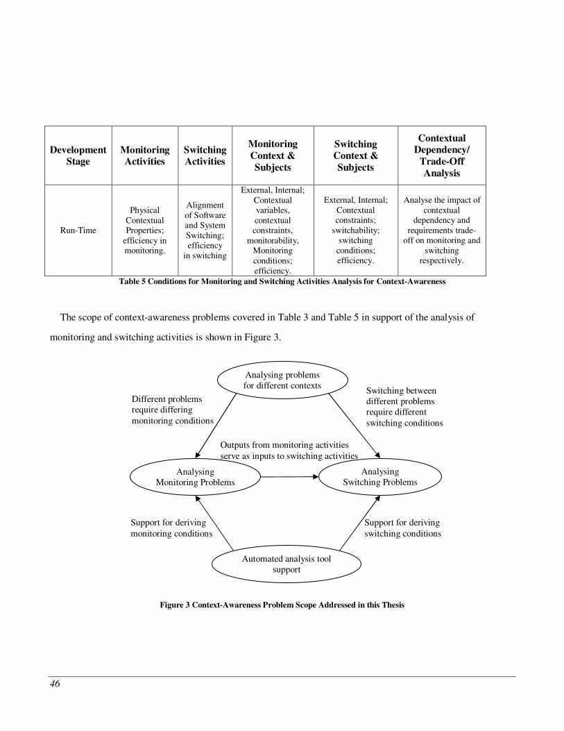
46
Development Stage
Monitoring Activities
Switching Activities
Monitoring Context & Subjects
Switching Context & Subjects
Contextual Dependency/
Trade-Off Analysis
Run-Time
Physical Contextual Properties;
efficiency in monitoring.
Alignment of Software and System Switching; efficiency
in switching
External, Internal; Contextual variables, contextual constraints,
monitorability, Monitoring conditions; efficiency.
External, Internal; Contextual constraints;
switchability; switching conditions; efficiency.
Analyse the impact of contextual
dependency and requirements trade-
off on monitoring and switching
respectively.
Table 5 Conditions for Monitoring and Switching Activities Analysis for Context-Awareness
The scope of context-awareness problems covered in Table 3 and Table 5 in support of the analysis of
monitoring and switching activities is shown in Figure 3.
Figure 3 Context-Awareness Problem Scope Addressed in this Thesis
Analysing problems for different contexts
Analysing Monitoring Problems
Analysing Switching Problems
Different problems require differing monitoring conditions
Switching between different problems require different switching conditions
Outputs from monitoring activities serve as inputs to switching activities
Automated analysis tool support
Support for deriving monitoring conditions
Support for deriving switching conditions
47
2.6 Chapter Summary
We have discussed fundamental concepts and basic definitions and used them to review related work in the
following four main areas: (1) variability analysis: - for the review on this, we focused on key motivations for
analysing variability in the widely used requirements engineering approaches. In addition, we also reviewed their
concepts for modelling and representing variability; (2) monitoring and switching analysis: - the review here was
focused on the use of monitoring and switching in checking for requirements inconsistency, execution failure
diagnostics, software compliance testing, performance tuning, ubiquitous computing, and self-managing. In line
with other researchers, we argued that the focus of current approaches is on monitoring requirements satisfaction
based on the outcome of application execution, and in switching application behaviour to satisfy different
requirements. Therefore, unforeseen requirements violations caused by changes in the physical context may
remain unnoticed. For approaches aiming to analyse self-managing systems, we argue that current focus is on
architectural reconfiguration at deployment-time, which results in the difficult problems of switching application
behaviour during run-time and that of physical context monitoring remaining unaddressed; (3) problem
description: - we reviewed current approaches for analysing requirements’ problems, focusing on their ability to
capture problems in three descriptions: requirements, specifications, contexts. This is significant for problem
classification for different contexts and in analysing monitoring and switching problems for context-awareness;
and (4) tool support for automated analysis: - we reviewed current approaches that make use of SAT-Solvers to
develop automated analysis tools for variability, monitoring and switching problems. In concluding each
discussion, we provided comparison tables which highlighted the limitations of current approaches and conditions
for the analysis of context-awareness problems.

48
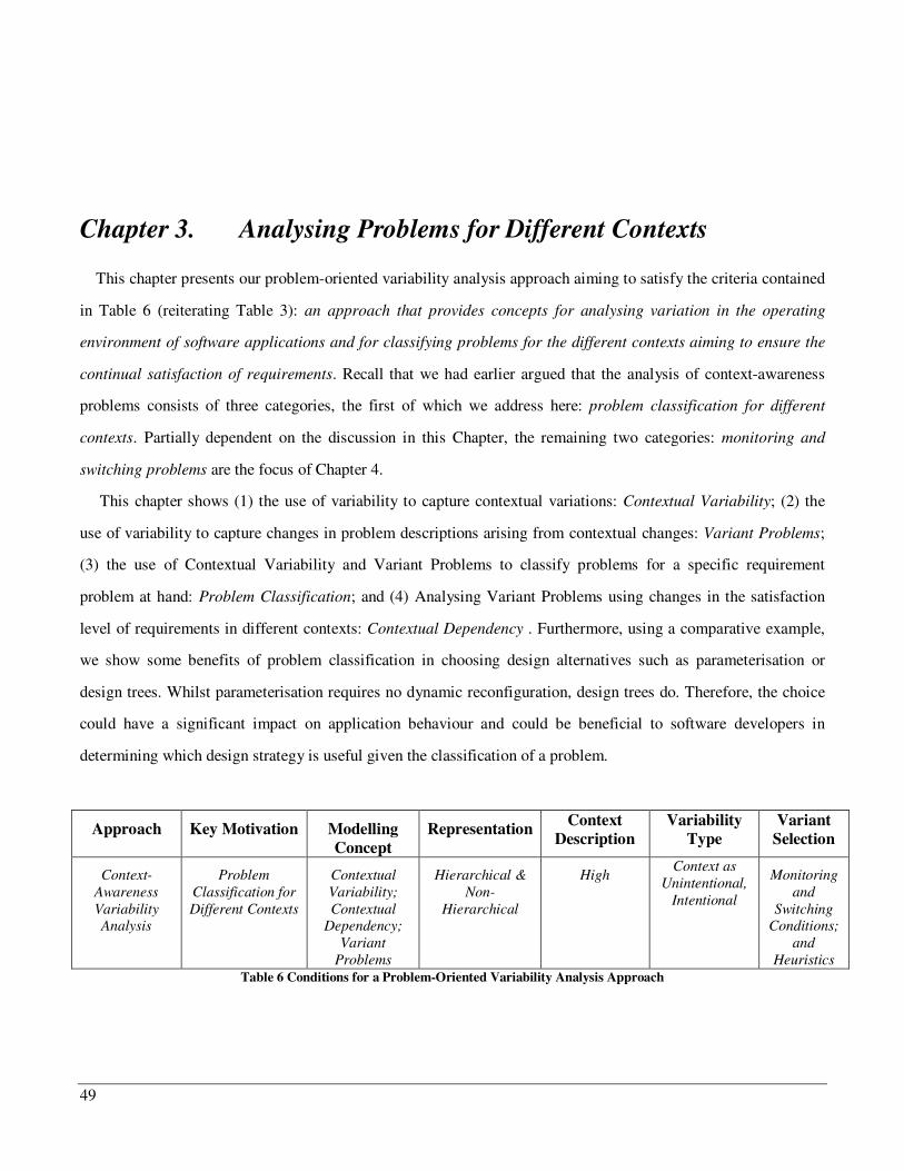
49
Chapter 3. Analysing Problems for Different Contexts
This chapter presents our problem-oriented variability analysis approach aiming to satisfy the criteria contained
in Table 6 (reiterating Table 3): an approach that provides concepts for analysing variation in the operating
environment of software applications and for classifying problems for the different contexts aiming to ensure the
continual satisfaction of requirements. Recall that we had earlier argued that the analysis of context-awareness
problems consists of three categories, the first of which we address here: problem classification for different
contexts. Partially dependent on the discussion in this Chapter, the remaining two categories: monitoring and
switching problems are the focus of Chapter 4.
This chapter shows (1) the use of variability to capture contextual variations: Contextual Variability; (2) the
use of variability to capture changes in problem descriptions arising from contextual changes: Variant Problems;
(3) the use of Contextual Variability and Variant Problems to classify problems for a specific requirement
problem at hand: Problem Classification; and (4) Analysing Variant Problems using changes in the satisfaction
level of requirements in different contexts: Contextual Dependency . Furthermore, using a comparative example,
we show some benefits of problem classification in choosing design alternatives such as parameterisation or
design trees. Whilst parameterisation requires no dynamic reconfiguration, design trees do. Therefore, the choice
could have a significant impact on application behaviour and could be beneficial to software developers in
determining which design strategy is useful given the classification of a problem.
Approach Key Motivation Modelling Concept
Representation Context
Description Variability
Type Variant
Selection
Context-Awareness Variability Analysis
Problem Classification for Different Contexts
Contextual Variability; Contextual
Dependency; Variant
Problems
Hierarchical & Non-
Hierarchical
High Context as
Unintentional, Intentional
Monitoring and
Switching Conditions;
and Heuristics
Table 6 Conditions for a Problem-Oriented Variability Analysis Approach
50
3.1 Facilitating Example
To facilitate the introduction of concepts and the illustration of their usefulness in analysing context-awareness
problems, we make use of a mobile device image transmission problem. The requirement R is stated as follows:
Software is to be specified to control the transmission of pictures from an external digital camera into a mobile
phone’s storage under the commands of a phone user. The overall requirements are stated as: a secure and
efficient transfer of pictures from a digital camera to the mobile phone’s storage.
Besides the functionality of transmitting pictures from the digital camera to the mobile phone, other issues to
be considered are security and performance of transmissions.
3.2 Variability in Application Contexts
Variability is a space of alternatives confined by possible values of a set of variables. In goal-based
requirements analysis approaches, the variables are stakeholder goals that can be OR-decomposed in a goal
model; in product-family development approaches, the variables are features that can be organised as optional or
alternative features in a feature tree. Extending this notion of variability, we define context variability as follows:
the subspace of variability that may result in different application behaviour in order to maintain the satisfaction
of requirements.
The obvious question arising from this definition is: how does one elicit the relevant contextual variables
whose changes can cause contextual variability? The remainder of this section aims to answer this question.
Figure 4 shows a problem description of the facilitating example which represents a typical problem frames
approach. By typical problem frames approach we mean, it assumes a fixed context of operation. Problem frames
approach focuses on how one can tell if the requirements are satisfied given the properties of the context that may
include the assumptions made of the context as well. By assuming that all potential listeners are authorised
(assumptions are usually not shown directly in problem frames descriptions), the focus is placed on assessing
whether the image is received and saved on the phone’s Internal Storage as shown by the requirements
constraining reference (indicated by an arrow from the requirement node to the domain node in the figure).
Alternatively, the context-awareness problem descriptions subjects contextual properties to further scrutiny by
asking if the assumptions could fail during application execution (which requires the assumptions to be made

51
explicit in the problem descriptions as shown in Figure 5) and if so the likely impact of such failures on the
satisfaction of R.
Figure 4 Non-Context-Awareness (Typical) Problem Diagram for Mobile Image Transmission
Figure 5 Context-Awareness Problem Diagram for Mobile Image Transmission3
3 Where R’ R and R’ R
Digital Camera
Controller
Internal Storage
User
R
C!{RequestTransmission, TerminateTransmission, RequestImageSize, ReceiveImageSizeInfo}
U!{Start, Stop}
IS!{Receive, Save} DC!{RequestTransmission, TerminateTransmission}
DC!{ConfirmStart, ConfirmStop}
IS!{Receive, Save}
U!{RequestTransmission, TerminateTransmission}
Digital Camera
Controller
Internal Storage
User
R’
C!{RequestTransmission, TerminateTransmission, RequestImageSize, ReceiveImageSizeInfo}
U!{Start, Stop}
IS!{Receive, Save}
Authorised Listener
DC!{RequestTransmission, TerminateTransmission}
DC!{ConfirmStart, ConfirmStop}
IS!{Receive, Save}
U!{RequestTransmission, TerminateTransmission}
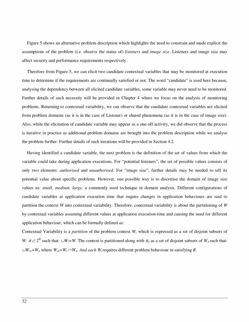
52
Figure 5 shows an alternative problem description which highlights the need to constrain and made explicit the
assumptions of the problem (i.e. observe the status of) listeners and image size. Listeners and image size may
affect security and performance requirements respectively.
Therefore from Figure 5, we can elicit two candidate contextual variables that may be monitored at execution
time to determine if the requirements are continually satisfied or not. The word “candidate” is used here because,
analysing the dependency between all elicited candidate variables, some variable may never need to be monitored.
Further details of such necessity will be provided in Chapter 4 where we focus on the analysis of monitoring
problems. Returning to contextual variability, we can observe that the candidate contextual variables are elicited
from problem domains (as it is in the case of Listener) or shared phenomena (as it is in the case of image size).
Also, while the elicitation of candidate variable may appear as a one-off activity, we did observe that the process
is iterative in practice as additional problem domains are brought into the problem description while we analyse
the problem further. Further details of such iterations will be provided in Section 4.2.
Having identified a candidate variable, the next problem is the definition of the set of values from which the
variable could take during application executions. For “potential listeners”, the set of possible values consists of
only two elements: authorised and unauthorised. For “image size”, further details may be needed to tell its
potential value about specific problems. However, one possible way is to discretise the domain of image size
values as: small, medium, large, a commonly used technique in domain analysis. Different configurations of
candidate variables at application execution time that require changes in application behaviours are said to
partition the context W into contextual variability. Therefore, contextual variability is about the partitioning of W
by contextual variables assuming different values at application execution-time and causing the need for different
application behaviour, which can be formally defined as:
Contextual Variability is a partition of the problem context W, which is expressed as a set of disjoint subsets of
W: ! " 2W such that: #Wi=W. The context is partitioned along with ! as a set of disjoint subsets of W such that:
#Wi=W where Wi=Wi $ W. And each Wi requires different problem behaviour in satisfying R.
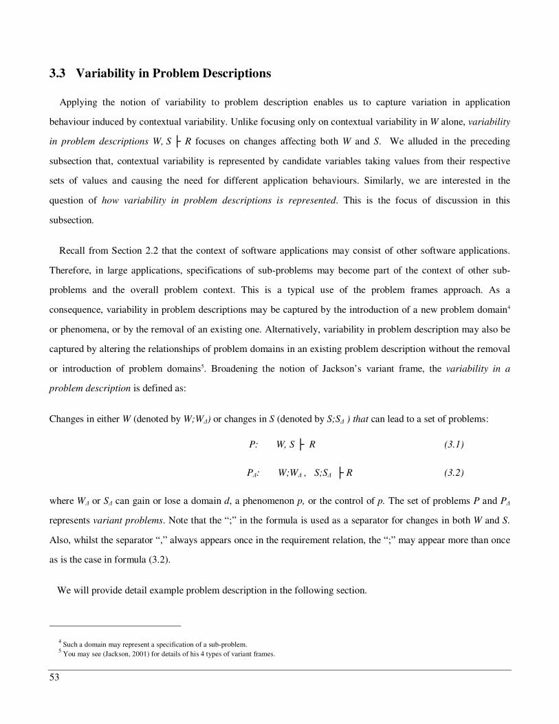
53
3.3 Variability in Problem Descriptions
Applying the notion of variability to problem description enables us to capture variation in application
behaviour induced by contextual variability. Unlike focusing only on contextual variability in W alone, variability
in problem descriptions W, S R focuses on changes affecting both W and S. We alluded in the preceding
subsection that, contextual variability is represented by candidate variables taking values from their respective
sets of values and causing the need for different application behaviours. Similarly, we are interested in the
question of how variability in problem descriptions is represented. This is the focus of discussion in this
subsection.
Recall from Section 2.2 that the context of software applications may consist of other software applications.
Therefore, in large applications, specifications of sub-problems may become part of the context of other sub-
problems and the overall problem context. This is a typical use of the problem frames approach. As a
consequence, variability in problem descriptions may be captured by the introduction of a new problem domain4
or phenomena, or by the removal of an existing one. Alternatively, variability in problem description may also be
captured by altering the relationships of problem domains in an existing problem description without the removal
or introduction of problem domains5. Broadening the notion of Jackson’s variant frame, the variability in a
problem description is defined as:
Changes in either W (denoted by W;W) or changes in S (denoted by S;S ) that can lead to a set of problems:
P: W, S R (3.1)
P: W;W , S;S R (3.2)
where W or S can gain or lose a domain d, a phenomenon p, or the control of p. The set of problems P and P
represents variant problems. Note that the “;” in the formula is used as a separator for changes in both W and S.
Also, whilst the separator “,” always appears once in the requirement relation, the “;” may appear more than once
as is the case in formula (3.2).
We will provide detail example problem description in the following section.
4 Such a domain may represent a specification of a sub-problem.
5 You may see (Jackson, 2001) for details of his 4 types of variant frames.
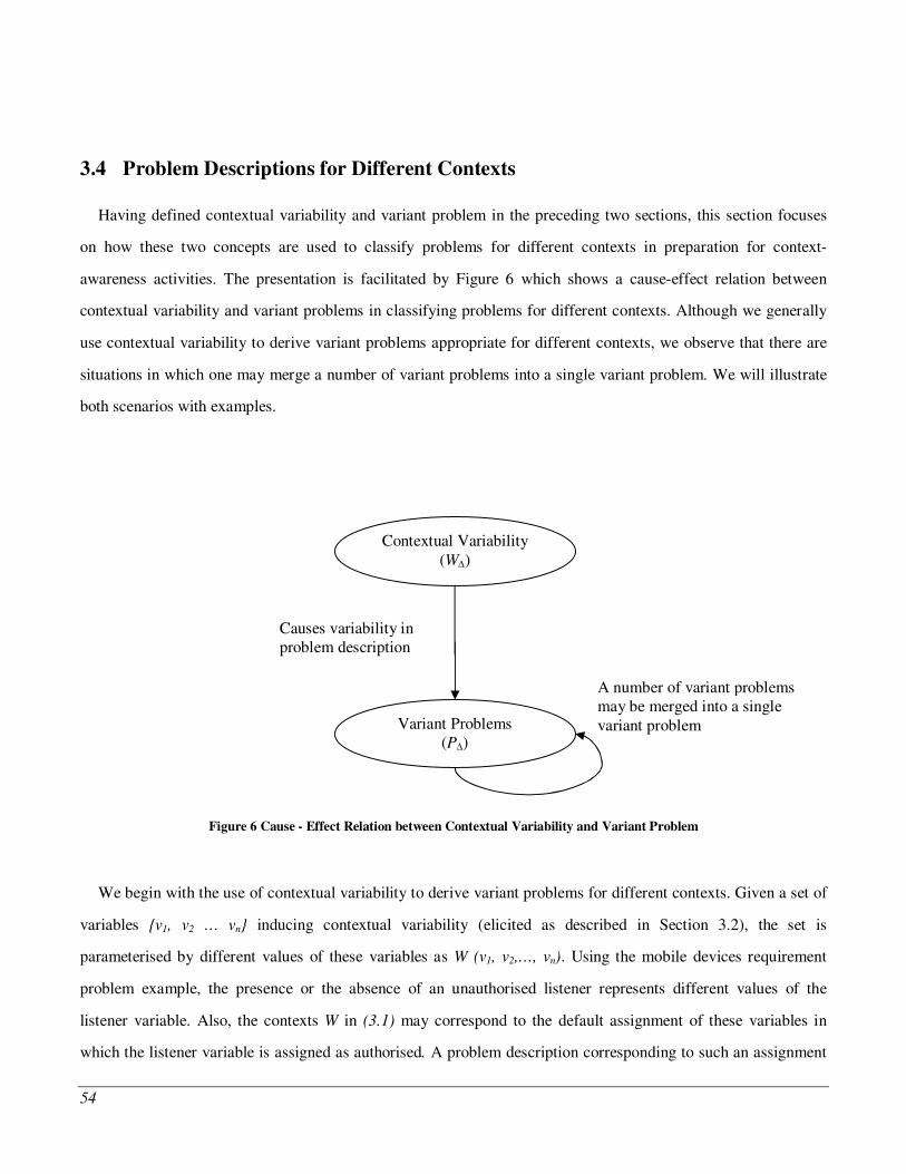
54
3.4 Problem Descriptions for Different Contexts
Having defined contextual variability and variant problem in the preceding two sections, this section focuses
on how these two concepts are used to classify problems for different contexts in preparation for context-
awareness activities. The presentation is facilitated by Figure 6 which shows a cause-effect relation between
contextual variability and variant problems in classifying problems for different contexts. Although we generally
use contextual variability to derive variant problems appropriate for different contexts, we observe that there are
situations in which one may merge a number of variant problems into a single variant problem. We will illustrate
both scenarios with examples.
Figure 6 Cause - Effect Relation between Contextual Variability and Variant Problem
We begin with the use of contextual variability to derive variant problems for different contexts. Given a set of
variables {v1, v2 … vn} inducing contextual variability (elicited as described in Section 3.2), the set is
parameterised by different values of these variables as W (v1, v2,…, vn). Using the mobile devices requirement
problem example, the presence or the absence of an unauthorised listener represents different values of the
listener variable. Also, the contexts W in (3.1) may correspond to the default assignment of these variables in
which the listener variable is assigned as authorised. A problem description corresponding to such an assignment
Contextual Variability (W)
Variant Problems (P)
Causes variability in problem description
A number of variant problems may be merged into a single variant problem
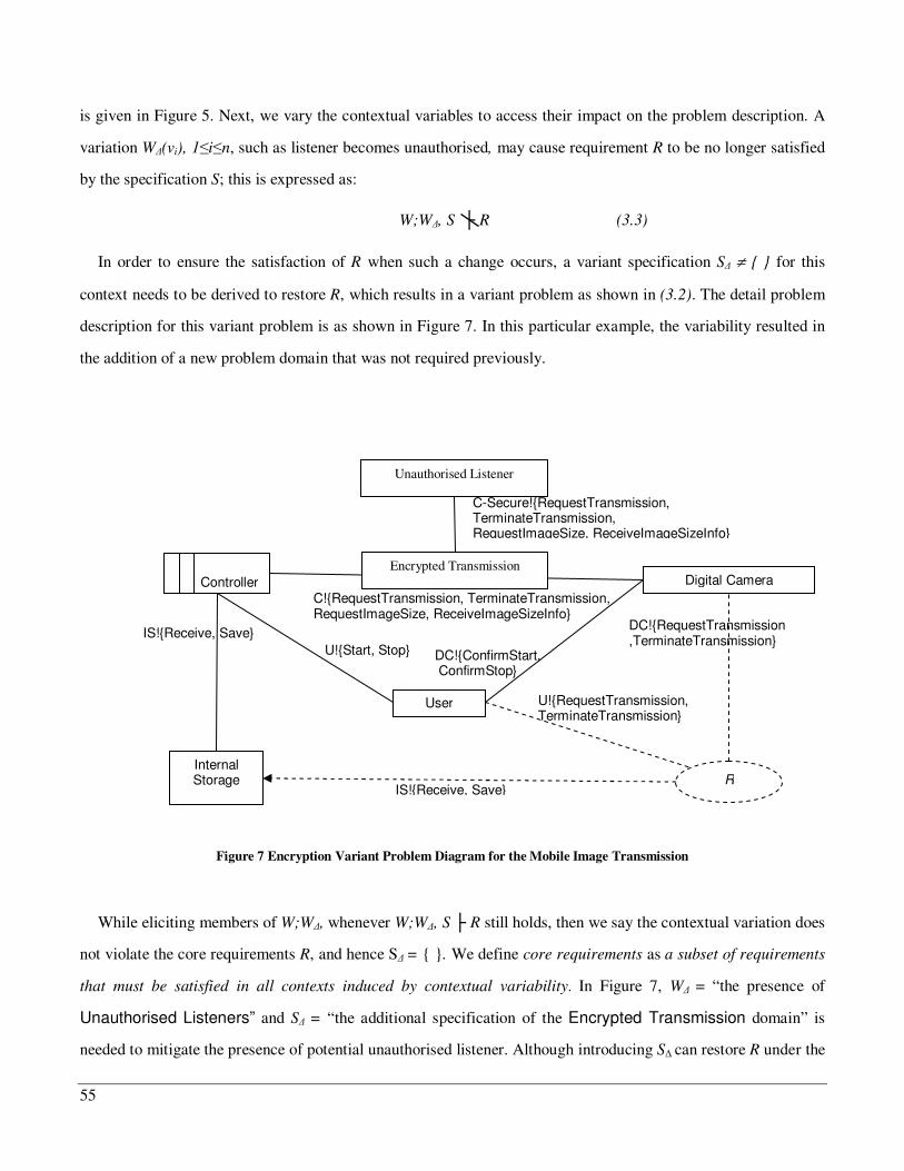
55
is given in Figure 5. Next, we vary the contextual variables to access their impact on the problem description. A
variation W(vi), 1in, such as listener becomes unauthorised, may cause requirement R to be no longer satisfied
by the specification S; this is expressed as:
W;W, S R (3.3)
In order to ensure the satisfaction of R when such a change occurs, a variant specification S % { } for this
context needs to be derived to restore R, which results in a variant problem as shown in (3.2). The detail problem
description for this variant problem is as shown in Figure 7. In this particular example, the variability resulted in
the addition of a new problem domain that was not required previously.
Figure 7 Encryption Variant Problem Diagram for the Mobile Image Transmission
While eliciting members of W;W, whenever W;W, S R still holds, then we say the contextual variation does
not violate the core requirements R, and hence S = { }. We define core requirements as a subset of requirements
that must be satisfied in all contexts induced by contextual variability. In Figure 7, W = “the presence of
Unauthorised Listeners” and S = “the additional specification of the Encrypted Transmission domain” is
needed to mitigate the presence of potential unauthorised listener. Although introducing S can restore R under the
Digital Camera
Controller
Internal Storage
User
R
C!{RequestTransmission, TerminateTransmission, RequestImageSize, ReceiveImageSizeInfo}
U!{Start, Stop} IS!{Receive, Save}
Unauthorised Listener
DC!{RequestTransmission,TerminateTransmission} DC!{ConfirmStart,
ConfirmStop}
IS!{Receive, Save}
U!{RequestTransmission, TerminateTransmission}
Encrypted Transmission
C-Secure!{RequestTransmission, TerminateTransmission, RequestImageSize, ReceiveImageSizeInfo}
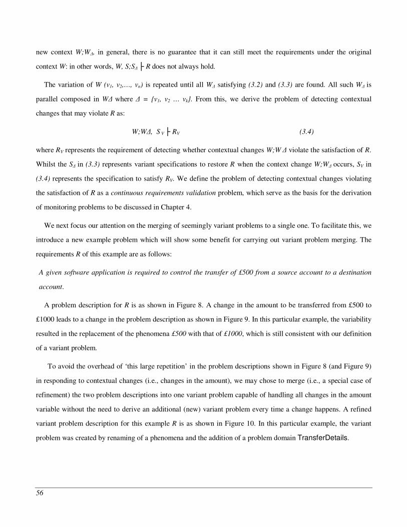
56
new context W;W, in general, there is no guarantee that it can still meet the requirements under the original
context W: in other words, W, S;S R does not always hold.
The variation of W (v1, v2,…, vn) is repeated until all W satisfying (3.2) and (3.3) are found. All such W is
parallel composed in W where = {v1, v2 … vk}. From this, we derive the problem of detecting contextual
changes that may violate R as:
W;W, S V RV (3.4)
where RV represents the requirement of detecting whether contextual changes W;W violate the satisfaction of R.
Whilst the S in (3.3) represents variant specifications to restore R when the context change W;W occurs, SV in
(3.4) represents the specification to satisfy RV. We define the problem of detecting contextual changes violating
the satisfaction of R as a continuous requirements validation problem, which serve as the basis for the derivation
of monitoring problems to be discussed in Chapter 4.
We next focus our attention on the merging of seemingly variant problems to a single one. To facilitate this, we
introduce a new example problem which will show some benefit for carrying out variant problem merging. The
requirements R of this example are as follows:
A given software application is required to control the transfer of £500 from a source account to a destination
account.
A problem description for R is as shown in Figure 8. A change in the amount to be transferred from £500 to
£1000 leads to a change in the problem description as shown in Figure 9. In this particular example, the variability
resulted in the replacement of the phenomena £500 with that of £1000, which is still consistent with our definition
of a variant problem.
To avoid the overhead of ‘this large repetition’ in the problem descriptions shown in Figure 8 (and Figure 9)
in responding to contextual changes (i.e., changes in the amount), we may chose to merge (i.e., a special case of
refinement) the two problem descriptions into one variant problem capable of handling all changes in the amount
variable without the need to derive an additional (new) variant problem every time a change happens. A refined
variant problem description for this example R is as shown in Figure 10. In this particular example, the variant
problem was created by renaming of a phenomena and the addition of a problem domain TransferDetails.
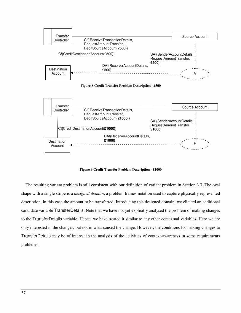
57
Figure 8 Credit Transfer Problem Description - £500
Figure 9 Credit Transfer Problem Description - £1000
The resulting variant problem is still consistent with our definition of variant problem in Section 3.3. The oval
shape with a single stripe is a designed domain, a problem frames notation used to capture physically represented
description, in this case the amount to be transferred. Introducing this designed domain, we elicited an additional
candidate variable TransferDetails. Note that we have not yet explicitly analysed the problem of making changes
to the TransferDetails variable. Hence, we have treated it similar to any other contextual variables. Here we are
only interested in the changes, but not in what caused the change. However, the conditions for making changes to
TransferDetails may be of interest in the analysis of the activities of context-awareness in some requirements
problems.
Source Account
Transfer
Controller
Destination Account
R
C!{ ReceiveTransactionDetails, RequestAmountTransfer, DebitSourceAccount(£1000)}
C!{CreditDestinationAccount(£1000)}
SA!{SenderAccountDetails, RequestAmountTransfer £1000}
DA!{ReceiverAccountDetails, £1000}
Source Account
Transfer
Controller
Destination Account R
C!{ ReceiveTransactionDetails, RequestAmountTransfer, DebitSourceAccount(£500)}
C!{CreditDestinationAccount(£500)} SA!{SenderAccountDetails, RequestAmountTransfer, £500} DA!{ReceiverAccountDetails,
£500}
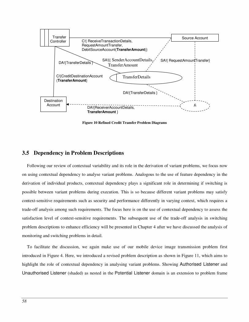
58
Figure 10 Refined Credit Transfer Problem Diagrams
3.5 Dependency in Problem Descriptions
Following our review of contextual variability and its role in the derivation of variant problems, we focus now
on using contextual dependency to analyse variant problems. Analogous to the use of feature dependency in the
derivation of individual products, contextual dependency plays a significant role in determining if switching is
possible between variant problems during execution. This is so because different variant problems may satisfy
context-sensitive requirements such as security and performance differently in varying context, which requires a
trade-off analysis among such requirements. The focus here is on the use of contextual dependency to assess the
satisfaction level of context-sensitive requirements. The subsequent use of the trade-off analysis in switching
problem descriptions to enhance efficiency will be presented in Chapter 4 after we have discussed the analysis of
monitoring and switching problems in detail.
To facilitate the discussion, we again make use of our mobile device image transmission problem first
introduced in Figure 4. Here, we introduced a revised problem description as shown in Figure 11, which aims to
highlight the role of contextual dependency in analysing variant problems. Showing Authorised Listener and
Unauthorised Listener (shaded) as nested in the Potential Listener domain is an extension to problem frame
Source Account
Transfer
Controller
Destination Account R
C!{ ReceiveTransactionDetails, RequestAmountTransfer, DebitSourceAccount(TransferAmount)}
C!{CreditDestinationAccount (TransferAmount}
SA!{ RequestAmountTransfer}
DA!{ReceiverAccountDetails, TransferAmount }
TransferDetails
SA!{( SenderAccountDetails, TransferAmount }
DA!{TransferDetails }
DA!{TransferDetails }
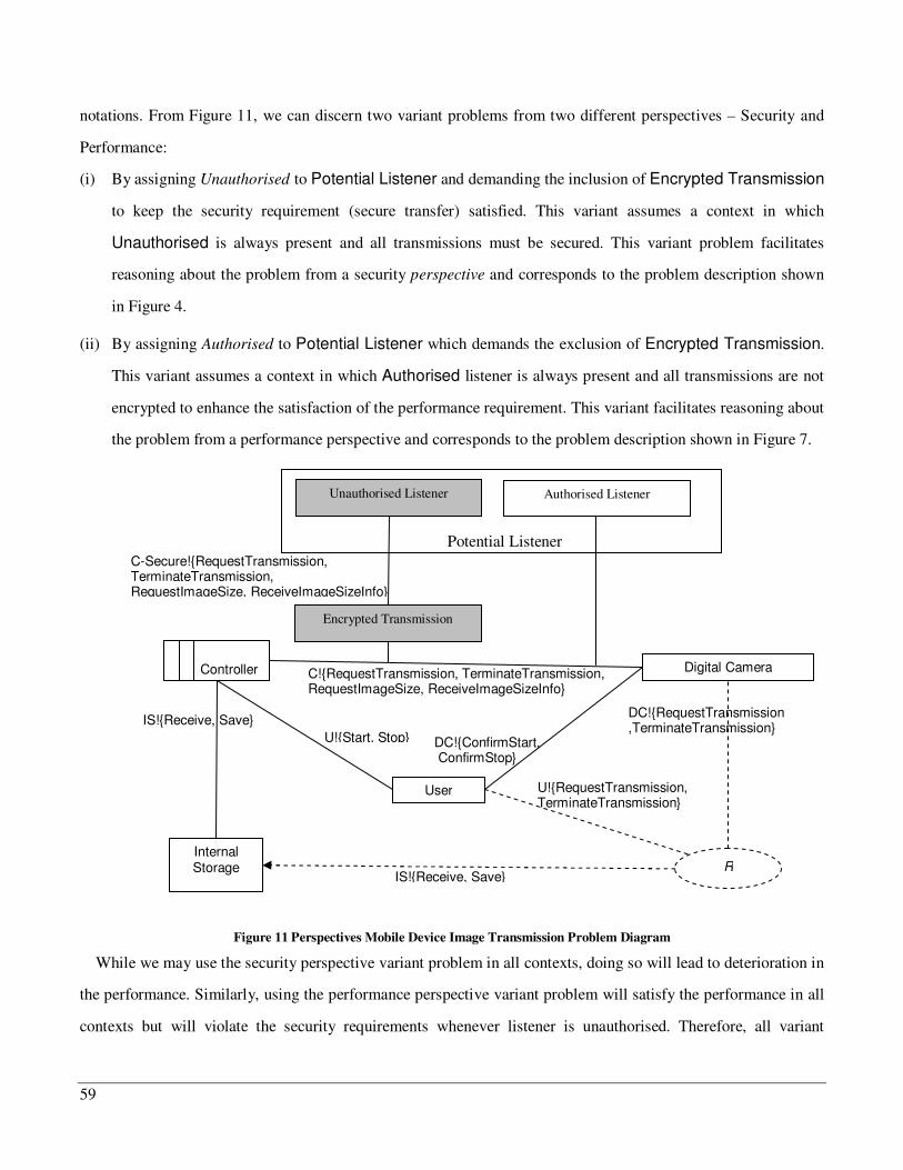
59
notations. From Figure 11, we can discern two variant problems from two different perspectives – Security and
Performance:
(i) By assigning Unauthorised to Potential Listener and demanding the inclusion of Encrypted Transmission
to keep the security requirement (secure transfer) satisfied. This variant assumes a context in which
Unauthorised is always present and all transmissions must be secured. This variant problem facilitates
reasoning about the problem from a security perspective and corresponds to the problem description shown
in Figure 4.
(ii) By assigning Authorised to Potential Listener which demands the exclusion of Encrypted Transmission.
This variant assumes a context in which Authorised listener is always present and all transmissions are not
encrypted to enhance the satisfaction of the performance requirement. This variant facilitates reasoning about
the problem from a performance perspective and corresponds to the problem description shown in Figure 7.
Figure 11 Perspectives Mobile Device Image Transmission Problem Diagram
While we may use the security perspective variant problem in all contexts, doing so will lead to deterioration in
the performance. Similarly, using the performance perspective variant problem will satisfy the performance in all
contexts but will violate the security requirements whenever listener is unauthorised. Therefore, all variant
Potential Listener
Digital Camera
Controller
Internal Storage
User
R
C!{RequestTransmission, TerminateTransmission, RequestImageSize, ReceiveImageSizeInfo}
U!{Start, Stop}
IS!{Receive, Save}
Unauthorised Listener
DC!{RequestTransmission,TerminateTransmission} DC!{ConfirmStart,
ConfirmStop}
IS!{Receive, Save}
U!{RequestTransmission, TerminateTransmission}
Encrypted Transmission
C-Secure!{RequestTransmission, TerminateTransmission, RequestImageSize, ReceiveImageSizeInfo}
Authorised Listener
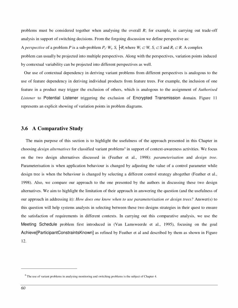
60
problems must be considered together when analysing the overall R; for example, in carrying out trade-off
analysis in support of switching decisions. From the forgoing discussion we define perspective as:
A perspective of a problem P is a sub-problem Pi: Wi, Si Ri where Wi " W, Si " S and Ri " R. A complex
problem can usually be projected into multiple perspectives. Along with the perspectives, variation points induced
by contextual variability can be projected into different perspectives as well.
Our use of contextual dependency in deriving variant problems from different perspectives is analogous to the
use of feature dependency in deriving individual products from feature trees. For example, the inclusion of one
feature in a product may trigger the exclusion of others, which is analogous to the assignment of Authorised
Listener to Potential Listener triggering the exclusion of Encrypted Transmission domain. Figure 11
represents an explicit showing of variation points in problem diagrams.
3.6 A Comparative Study
The main purpose of this section is to highlight the usefulness of the approach presented in this Chapter in
choosing design alternatives for classified variant problems6 in support of context-awareness activities. We focus
on the two design alternatives discussed in (Feather et al., 1998): parameterisation and design tree.
Parameterisation is when application behaviour is changed by adjusting the value of a control parameter while
design tree is when the behaviour is changed by selecting a different control strategy altogether (Feather et al.,
1998). Also, we compare our approach to the one presented by the authors in discussing these two design
alternatives. We aim to highlight the limitation of their approach in answering the question (and the usefulness of
our approach in addressing it): How does one know when to use parameterisation or design trees? Answer(s) to
this question will help systems analysts in selecting between these two designs strategies in their quest to ensure
the satisfaction of requirements in different contexts. In carrying out this comparative analysis, we use the
Meeting Schedule problem first introduced in (Van Lamsweerde et al., 1995), focusing on the goal
Achieve[ParticipantConstraintsKnown] as refined by Feather et al and described by them as shown in Figure
12.
6 The use of variant problems in analysing monitoring and switching problems is the subject of Chapter 4.
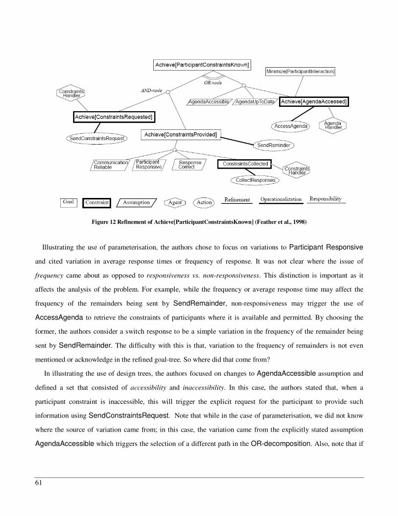
61
Figure 12 Refinement of Achieve[ParticipantConstraintsKnown] (Feather et al., 1998)
Illustrating the use of parameterisation, the authors chose to focus on variations to Participant Responsive
and cited variation in average response times or frequency of response. It was not clear where the issue of
frequency came about as opposed to responsiveness vs. non-responsiveness. This distinction is important as it
affects the analysis of the problem. For example, while the frequency or average response time may affect the
frequency of the remainders being sent by SendRemainder, non-responsiveness may trigger the use of
AccessAgenda to retrieve the constraints of participants where it is available and permitted. By choosing the
former, the authors consider a switch response to be a simple variation in the frequency of the remainder being
sent by SendRemainder. The difficulty with this is that, variation to the frequency of remainders is not even
mentioned or acknowledge in the refined goal-tree. So where did that come from?
In illustrating the use of design trees, the authors focused on changes to AgendaAccessible assumption and
defined a set that consisted of accessibility and inaccessibility. In this case, the authors stated that, when a
participant constraint is inaccessible, this will trigger the explicit request for the participant to provide such
information using SendConstraintsRequest. Note that while in the case of parameterisation, we did not know
where the source of variation came from; in this case, the variation came from the explicitly stated assumption
AgendaAccessible which triggers the selection of a different path in the OR-decomposition. Also, note that if
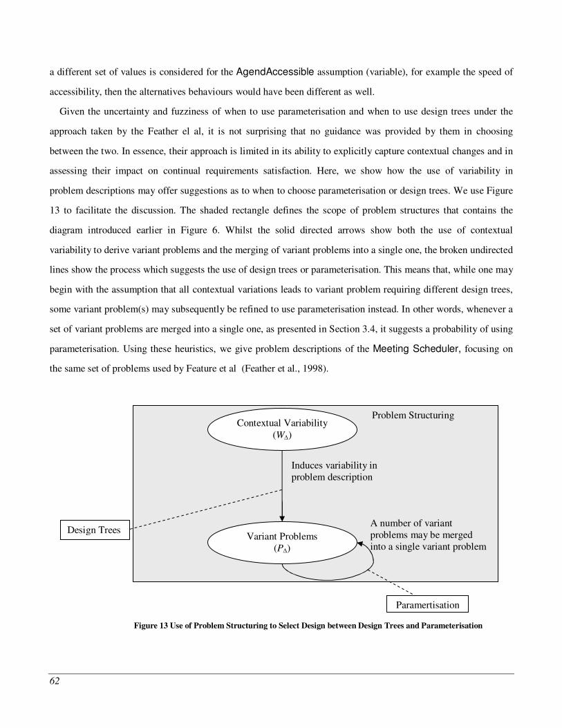
62
a different set of values is considered for the AgendAccessible assumption (variable), for example the speed of
accessibility, then the alternatives behaviours would have been different as well.
Given the uncertainty and fuzziness of when to use parameterisation and when to use design trees under the
approach taken by the Feather el al, it is not surprising that no guidance was provided by them in choosing
between the two. In essence, their approach is limited in its ability to explicitly capture contextual changes and in
assessing their impact on continual requirements satisfaction. Here, we show how the use of variability in
problem descriptions may offer suggestions as to when to choose parameterisation or design trees. We use Figure
13 to facilitate the discussion. The shaded rectangle defines the scope of problem structures that contains the
diagram introduced earlier in Figure 6. Whilst the solid directed arrows show both the use of contextual
variability to derive variant problems and the merging of variant problems into a single one, the broken undirected
lines show the process which suggests the use of design trees or parameterisation. This means that, while one may
begin with the assumption that all contextual variations leads to variant problem requiring different design trees,
some variant problem(s) may subsequently be refined to use parameterisation instead. In other words, whenever a
set of variant problems are merged into a single one, as presented in Section 3.4, it suggests a probability of using
parameterisation. Using these heuristics, we give problem descriptions of the Meeting Scheduler, focusing on
the same set of problems used by Feature et al (Feather et al., 1998).
Figure 13 Use of Problem Structuring to Select Design between Design Trees and Parameterisation
Problem Structuring Contextual Variability
(W)
Variant Problems (P)
Induces variability in problem description
A number of variant problems may be merged into a single variant problem
Design Trees
Paramertisation
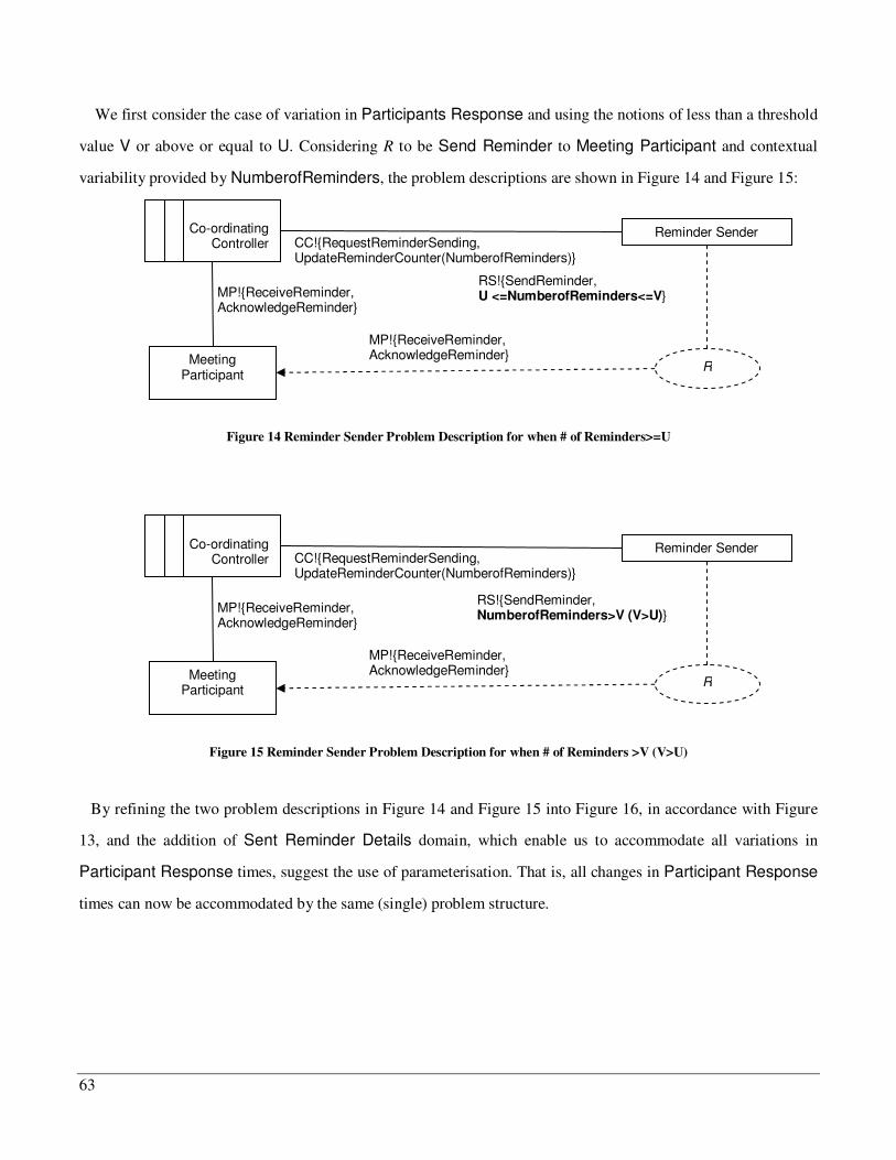
63
We first consider the case of variation in Participants Response and using the notions of less than a threshold
value V or above or equal to U. Considering R to be Send Reminder to Meeting Participant and contextual
variability provided by NumberofReminders, the problem descriptions are shown in Figure 14 and Figure 15:
Figure 14 Reminder Sender Problem Description for when # of Reminders>=U
Figure 15 Reminder Sender Problem Description for when # of Reminders >V (V>U)
By refining the two problem descriptions in Figure 14 and Figure 15 into Figure 16, in accordance with Figure
13, and the addition of Sent Reminder Details domain, which enable us to accommodate all variations in
Participant Response times, suggest the use of parameterisation. That is, all changes in Participant Response
times can now be accommodated by the same (single) problem structure.
Reminder Sender
Co-ordinating
Controller
Meeting Participant
R
CC!{RequestReminderSending, UpdateReminderCounter(NumberofReminders)}
MP!{ReceiveReminder, AcknowledgeReminder}
RS!{SendReminder, NumberofReminders>V (V>U)}
MP!{ReceiveReminder, AcknowledgeReminder}
Reminder Sender
Co-ordinating
Controller
Meeting Participant
R
CC!{RequestReminderSending, UpdateReminderCounter(NumberofReminders)}
MP!{ReceiveReminder, AcknowledgeReminder}
RS!{SendReminder, U <=NumberofReminders<=V}
MP!{ReceiveReminder, AcknowledgeReminder}
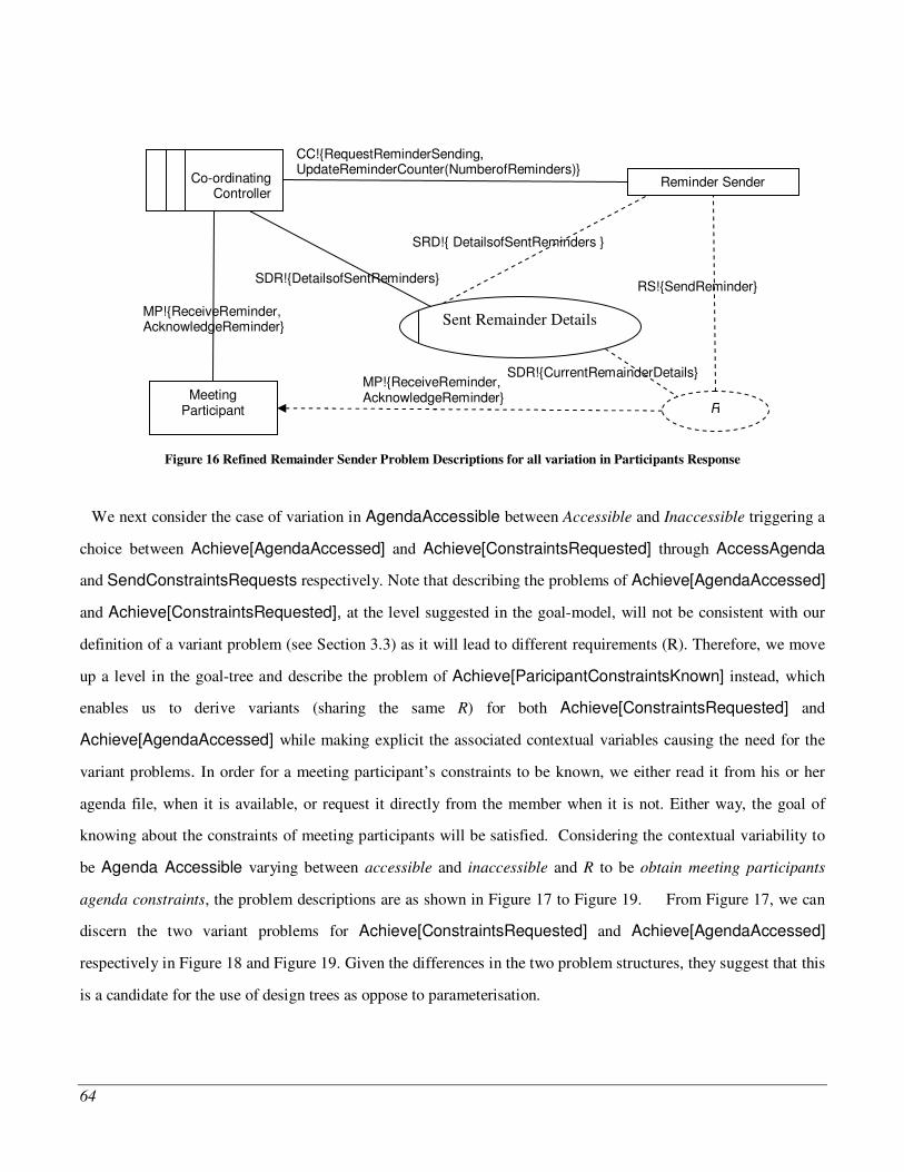
64
Figure 16 Refined Remainder Sender Problem Descriptions for all variation in Participants Response
We next consider the case of variation in AgendaAccessible between Accessible and Inaccessible triggering a
choice between Achieve[AgendaAccessed] and Achieve[ConstraintsRequested] through AccessAgenda
and SendConstraintsRequests respectively. Note that describing the problems of Achieve[AgendaAccessed]
and Achieve[ConstraintsRequested], at the level suggested in the goal-model, will not be consistent with our
definition of a variant problem (see Section 3.3) as it will lead to different requirements (R). Therefore, we move
up a level in the goal-tree and describe the problem of Achieve[ParicipantConstraintsKnown] instead, which
enables us to derive variants (sharing the same R) for both Achieve[ConstraintsRequested] and
Achieve[AgendaAccessed] while making explicit the associated contextual variables causing the need for the
variant problems. In order for a meeting participant’s constraints to be known, we either read it from his or her
agenda file, when it is available, or request it directly from the member when it is not. Either way, the goal of
knowing about the constraints of meeting participants will be satisfied. Considering the contextual variability to
be Agenda Accessible varying between accessible and inaccessible and R to be obtain meeting participants
agenda constraints, the problem descriptions are as shown in Figure 17 to Figure 19. From Figure 17, we can
discern the two variant problems for Achieve[ConstraintsRequested] and Achieve[AgendaAccessed]
respectively in Figure 18 and Figure 19. Given the differences in the two problem structures, they suggest that this
is a candidate for the use of design trees as oppose to parameterisation.
Reminder Sender
Co-ordinating
Controller
Meeting Participant R
CC!{RequestReminderSending, UpdateReminderCounter(NumberofReminders)}
MP!{ReceiveReminder, AcknowledgeReminder}
RS!{SendReminder}
MP!{ReceiveReminder, AcknowledgeReminder}
Sent Remainder Details
SRD!{ DetailsofSentReminders }
SDR!{DetailsofSentReminders}
SDR!{CurrentRemainderDetails}
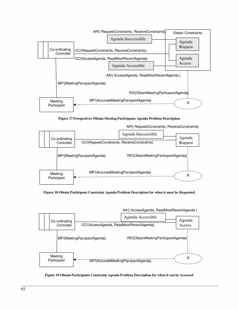
65
Figure 17 Perspectives Obtain Meeting Participants Agenda Problem Description
Figure 18 Obtain Participant Constraint Agenda Problem Description for when it must be Requested
Figure 19 Obtain Participants Constraint Agenda Problem Description for when it can be Accessed
Meeting Participant
R
CC!{AccessAgenda, ReadMostRecentAgenda}
MP!{MeetingParcipantAgenda} RS!{ObtainMeetingParticipantAgenda}
Agenda Access
Co-ordinating
Controller
MP!{AccurateMeetingParcipantAgenda}
Agenda Accessible
AA!{ AccessAgenda, ReadMostRecentAgenda }
Meeting Participant
R
CC!{RequestConstraints, ReceiveConstraints}
MP!{MeetingParcipantAgenda} RS!{ObtainMeetingParticipantAgenda}
Co-ordinating
Controller
MP!{AccurateMeetingParcipantAgenda}
Agenda Request
Agenda Inaccessible
AR!{ RequestConstraints, ReceiveConstraints}
Obtain Constraints
Meeting Participant
R
CC!{RequestConstraints, ReceiveConstraints}, CC!{AccessAgenda, ReadMostRecentAgenda}
MP!{MeetingParcipantAgenda}
RS!{ObtainMeetingParticipantAgenda}
Co-ordinating
Controller
MP!{AccurateMeetingParcipantAgenda}
Agenda Inaccessible
Agenda Accessible
Agenda Request
Agenda Access
AR!{ RequestConstraints, ReceiveConstraints}
AA!{ AccessAgenda, ReadMostRecentAgenda }
66
The ability to know when to choose between design trees and parameterisation is useful in the sense that, while
design trees require dynamic reconfiguration, parameterisation does not. Hence, both the complexity and
computational overhead in the latter are less in comparison to the former, as noted by Kramer et al (Kramer and
Magee, 2007).
3.7 Chapter Summary
In this chapter, we have presented our approach aiming to meet the criteria defined in Table 6: an approach that
provides concepts for analysing variation in the operating environment of software applications and for
classifying problems for the different contexts aiming to ensure the continual satisfaction of requirements. The
key motivation is problem classification (Section 3.4) in support of context-awareness analysis. We have
provided mechanisms for: (1) the use of variability to capture contextual variations which we defined as
Contextual Variability (Section 3.2); (2) the use of variability to capture changes in problem descriptions arising
from contextual changes which we defined as Variant Problems (Section 3.3); (3) the use of Contextual
Variability and Variant Problems to classify problems for a specific requirement problem at hand, in support of
context-awareness; and (4) Analyse Variant Problems using changes in the satisfaction levels of requirements in
different contexts which we defined as Contextual Dependency (Section 3.5). Furthermore, we have used a
comparative example (See Section 3.6) to show some benefits of problem classification in choosing design
alternatives such as parameterisation or design trees. Parameterisation is when application behaviour is changed
by adjusting the value of a control parameter while design tree is when the behaviour is changed by selecting a
different control strategy altogether. Also, whilst parameterisation requires no dynamic reconfiguration, design
trees do. Therefore, the choice could have a significant impact on application behaviour and could be beneficial to
software developers in determining which design strategy is useful given the characteristics of a problem. In terms
of the modelling hierarchy, we have illustrated how non-hierarchical problem descriptions is carried out (e.g., as
shown in Figure 14 and Figure 15), and that of hierarchical (e.g., as shown in Figure 11 and Figure 17). Finally,
we have also shown how contextual variability and variant problems are used to analyse contextual changes as
unintentional variability and that of the refinement of variant problems into other variants to manage intentional
variability by transforming seemingly changes in R to W (see Figure 8 to Figure 10).
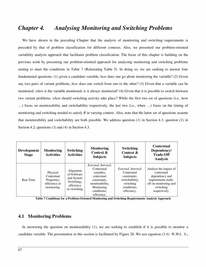
67
Chapter 4. Analysing Monitoring and Switching Problems
We have shown in the preceding Chapter that the analysis of monitoring and switching requirements is
preceded by that of problem classification for different contexts. Also, we presented our problem-oriented
variability analysis approach that facilitates problem classification. The focus of this chapter is building on the
previous work by presenting our problem-oriented approach for analysing monitoring and switching problems
aiming to meet the conditions in Table 7 (Reiterating Table 5). In doing so, we are seeking to answer four
fundamental questions: (1) given a candidate variable, how does one go about monitoring the variable? (2) Given
any two pairs of variant problems, how does one switch from one to the other? (3) Given that a variable can be
monitored, when is the variable monitored; is it always monitored? (4) Given that it is possible to switch between
two variant problems, when should switching activity take place? While the first two set of questions (i.e., how
…) focus on monitorability and switchability respectively, the last two (i.e., when …) focus on the timing of
monitoring and switching needed to satisfy R in varying context. Also, note that the latter set of questions assume
that monitorability and switchability are both possible. We address question (1) in Section 4.1; question (2) in
Section 4.2; questions (3) and (4) in Section 4.3.
Development Stage
Monitoring Activities
Switching Activities
Monitoring Context & Subjects
Switching Context & Subjects
Contextual Dependency/
Trade-Off Analysis
Run-Time
Physical Contextual Properties;
efficiency in monitoring.
Alignment of Software and System Switching; efficiency
in switching
External, Internal; Contextual variables, contextual constraints,
monitorability, Monitoring conditions; efficiency.
External, Internal; Contextual constraints;
switchability; switching conditions; efficiency.
Analyse the impact of contextual
dependency and requirements trade-
off on monitoring and switching
respectively.
Table 7 Conditions for a Problem-Oriented Monitoring and Switching Requirements Analysis Approach
4.1 Monitoring Problems
In answering the question on monitorability (1), we are seeking to establish if it is possible to monitor a
candidate variable. The presentation in this section is facilitated by Figure 20. We use equation (3.4): W;W, S V
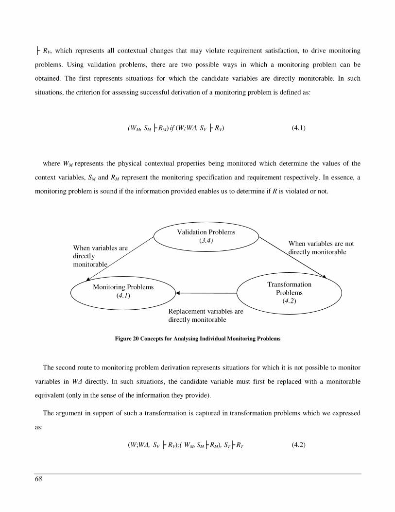
68
RV, which represents all contextual changes that may violate requirement satisfaction, to drive monitoring
problems. Using validation problems, there are two possible ways in which a monitoring problem can be
obtained. The first represents situations for which the candidate variables are directly monitorable. In such
situations, the criterion for assessing successful derivation of a monitoring problem is defined as:
(WM, SM RM) if (W;W, SV RV) (4.1)
where WM represents the physical contextual properties being monitored which determine the values of the
context variables, SM and RM represent the monitoring specification and requirement respectively. In essence, a
monitoring problem is sound if the information provided enables us to determine if R is violated or not.
Figure 20 Concepts for Analysing Individual Monitoring Problems
The second route to monitoring problem derivation represents situations for which it is not possible to monitor
variables in W directly. In such situations, the candidate variable must first be replaced with a monitorable
equivalent (only in the sense of the information they provide).
The argument in support of such a transformation is captured in transformation problems which we expressed
as:
(W;W, SV RV);( WM, SM RM), ST RT (4.2)
Validation Problems (3.4)
Monitoring Problems (4.1)
When variables are not directly monitorable
When variables are directly monitorable
Transformation Problems
(4.2)
Replacement variables are directly monitorable
69
where RT = (WM, SM RM) if (W;W, SV RV) and WM is monitorable and W not.
For the transformation of W in (3.4) to WM in (4.1) to be valid, we need to show that by observing WM one can
assess the satisfaction of R in the real world. A possible way of achieving this is to use structured argumentation
about trust assumptions (Haley et al., 2006) in the physical world with regards to the observed phenomena. For
example, given that all transmission listeners at secured locations are authorised, one can justifiably monitor
location (WM) and not potential listeners (W). If a change in trust assumption breaks (4.2), similarly to (3.3),
one needs to detect the change and restore the satisfaction of (4.2). In this sense, the transformation problem (4.2)
should be handled recursively as a context-awareness problem. Considering our example mobile device image
transmission problem (see Figure 4), the first path of monitoring problem derivation will be monitoring the
Image Size variable, which we can observe directly. The monitoring of Location instead of Potential Listener
represents the second path.
4.1.1 Directly Monitorable Variables
Having reviewed the two possible ways of deriving monitoring problems, we next take a detailed look at how a
monitoring problem is described using these paths. We first consider the case in which the candidate variable is
directly observable using the example problem of monitoring Image Size in our running mobile application
example. The image monitoring requirement Rm is defined as the reporting of the status of images size as either
being small, medium or large using the predefined lower band (L) and upper band (U). The image transmission
monitoring problem description is as shown in Figure 21. Given that the digital camera file system is a ‘formal’
physical domain (i.e., bits for the image file are physically stored on the magnetic disk) and reliability of the
magnetic disk technology is ‘good’, we choose not to investigate the reliability of the storage medium further.
This may not always be the case in other monitoring problem descriptions where the domains being monitored are
‘informal’.

70
Figure 21 Image Size Monitoring Problem Description
4.1.2 Indirectly Monitorable Variables
We next consider the situation in which the candidate variable is not directly observable or more ‘expensive’ to
do so. Making use of the mobile application example again, the other candidate variable is Potential Listener. A
possible monitoring problem description for potential listener is as shown in Figure 22. As highlighted in the
figure, the reliability of human observers raises serious concerns. In other words, it is not conceivable to have
human observers accompanying the mobile devices users everywhere. Therefore, a more plausible variable,
capable of providing equivalent information, is needed to replace Potential Listener.
Figure 22 Listener Status Monitoring Problem Description
Rm
PL!{ReportCurrentListenerStatus}
LM{UpdateStatusRecord(Authorised), UpdateStatusRecord(Unauthorised)}
Listener Monitor
Potential Listener
Listener Status
HPLO!{ReportAuthorisedListener, ReportUnauthorisedListener} LM!{ReceiveListenerStatusUpdate}
LS!{ListenerStatusReport}
Human Potential Listener Observer
HPLO!{ObserveListener, ReportStatus}
How reliable are human observers?
Rm
DCFS!{SendActiveImageFileSizeInfo}
ISM{UpdateImageRecord(Size >U) ,UpdateImageRecord( L< Size <U), UpdateImageRecord(Size < L)}
Image Size Monitor
Digital Camera File System
Image Size Status
ISM!{RequestActiveFileRecord, ReceiveActiveFileRecord} DCFS!{SendActiveFileRecord}
ISS!{CurrentImageFileReport}
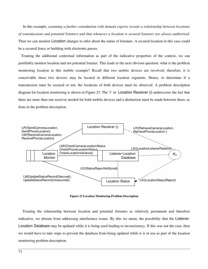
71
In this example, assuming a further consultation with domain experts reveals a relationship between locations
of transmissions and potential listeners and that whenever a location is secured listeners are always authorised.
Then we can monitor Location changes to infer about the status of listeners. A secured location in this case could
be a secured fence or building with electronic passes.
Treating the additional contextual information as part of the indicative properties of the context, we can
justifiably monitor location and not potential listener. This leads to the next obvious question: what is the problem
monitoring location in this mobile example? Recall that two mobile devices are involved; therefore, it is
conceivable these two devices may be located in different location segments. Hence, to determine if a
transmission must be secured or not, the locations of both devices must be observed. A problem description
diagram for location monitoring is shown in Figure 23. The ‘i’ in Location Receiver (i) underscores the fact that
there are more than one receiver needed for both mobile devices and a distinction must be made between these, as
done in the problem description.
Figure 23 Location Monitoring Problem Description
Treating the relationship between location and potential listeners as relatively permanent and therefore
indicative, we abstain from addressing interference issues. By this we mean, the possibility that the Listener-
Location Database may be updated while it is being used leading to inconsistency. If this was not the case, then
we would have to take steps to prevent the database from being updated while it is in use as part of the location
monitoring problem description.
Rm
LR!{RetrieveCameraLocation, RetrievePhoneLocation }
LM{UpdateStatusRecord(Secured), UpdateStatusRecord(Unsecured)}
Location Monitor
Location Status
LR!{SendCameraLocation, SendPhoneLocation} LM!{ReceiveCameraLocation, ReceivePhoneLocation}
LS!{LocationStatusReport}
Location Receiver (i)
LS!{StatusReportAsStored}
Listener-Location Database
LS!{LocationListenerRelation} LM!{CheckCameraLocationStatus CheckPhoneLocationStatus, CheckLocationVariance}
72
In summary, the aggregation of all information provided by all monitoring problems satisfy (4.1) or (4.1 and
4.2) when transformation problems are used to find replacement variables. The reliance of the indicative property
that there is a relationship between location and listeners and that all listeners at secured locations are authorised,
we meet the criteria defined in (4.2) in using Listener-Location Database to assist in monitoring location. This
is because, whenever location is secured, then the security requirement will always be satisfied. Conversely, when
location is not secured, then listeners may be unauthorised and transmissions must be secured through the use of
the problem description in Figure 7. Using Listener-Location Database makes explicit the use of a
transformation problem and shows that location is being monitored in place of potential listener. Contrasting the
image and potential listener/location problem descriptions, we have shown why the question of how does one
monitor a candidate variable is important and the need for detail problem description in answering such a
question.
4.2 Switching Problems
This section focuses on the question of switchability (2) that ensures the continual satisfaction of R. Taking the
properties of the context into consideration, we seek to synchronise both the software and system switching.
Given two variant problems, the individual switching problem between them is defined as:
W;W;S;S, Ss Rs (4.3)
Where W, S R and W;W, S;S R and Rs R.
We again make use of the mobile application example in illustrating the nature of such switching problems.
Considering the two variant problems for the mobile application problem shown in Figure 4 (Controller1) and
Figure 7 (Controller2), the single distinguishing activity between them is encryption. Therefore, the nature of the
encryption activity becomes the focal point in analysing the switching problem between the two variant problems
as it significantly affects Ss. The switching problem description for switching from Controller1 to Controller2 is
shown in Figure 24, while that of switching from Controller2 to Controller1 is shown in Figure 25. Making use
of the phenomena {Pause, Resume, Stop, Start} in both controllers, the switching machine can switch control
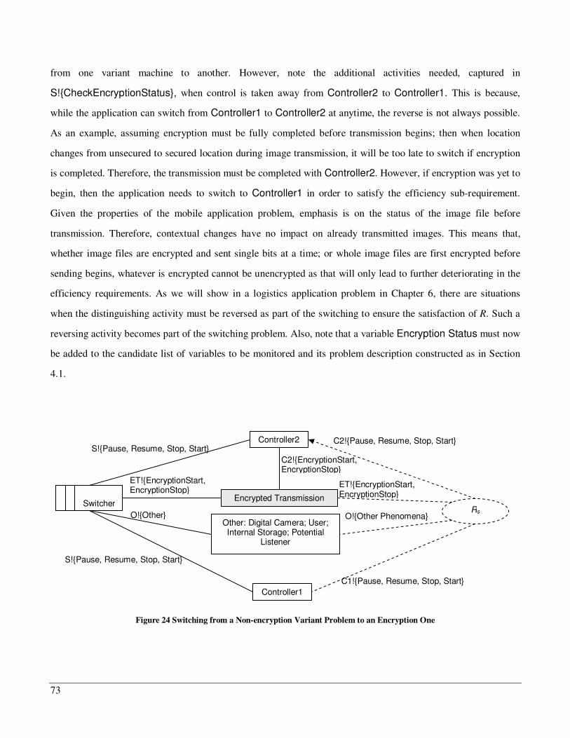
73
from one variant machine to another. However, note the additional activities needed, captured in
S!{CheckEncryptionStatus}, when control is taken away from Controller2 to Controller1. This is because,
while the application can switch from Controller1 to Controller2 at anytime, the reverse is not always possible.
As an example, assuming encryption must be fully completed before transmission begins; then when location
changes from unsecured to secured location during image transmission, it will be too late to switch if encryption
is completed. Therefore, the transmission must be completed with Controller2. However, if encryption was yet to
begin, then the application needs to switch to Controller1 in order to satisfy the efficiency sub-requirement.
Given the properties of the mobile application problem, emphasis is on the status of the image file before
transmission. Therefore, contextual changes have no impact on already transmitted images. This means that,
whether image files are encrypted and sent single bits at a time; or whole image files are first encrypted before
sending begins, whatever is encrypted cannot be unencrypted as that will only lead to further deteriorating in the
efficiency requirements. As we will show in a logistics application problem in Chapter 6, there are situations
when the distinguishing activity must be reversed as part of the switching to ensure the satisfaction of R. Such a
reversing activity becomes part of the switching problem. Also, note that a variable Encryption Status must now
be added to the candidate list of variables to be monitored and its problem description constructed as in Section
4.1.
Figure 24 Switching from a Non-encryption Variant Problem to an Encryption One
Switcher
Encrypted Transmission
Rs
Controller2
Controller1
Other: Digital Camera; User; Internal Storage; Potential
Listener
C1!{Pause, Resume, Stop, Start}
O!{Other Phenomena}
ET!{EncryptionStart, EncryptionStop}
C2!{Pause, Resume, Stop, Start}
O!{Other}
C2!{EncryptionStart, EncryptionStop}
ET!{EncryptionStart, EncryptionStop}
S!{Pause, Resume, Stop, Start}
S!{Pause, Resume, Stop, Start}
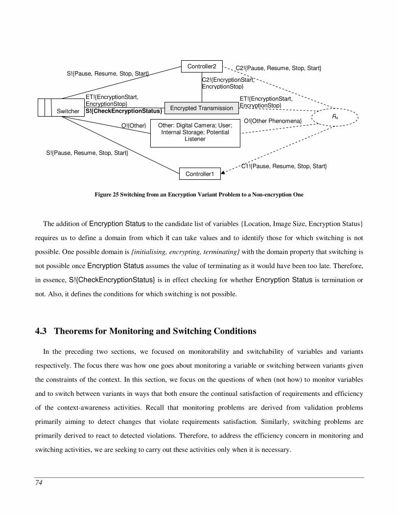
74
Figure 25 Switching from an Encryption Variant Problem to a Non-encryption One
The addition of Encryption Status to the candidate list of variables {Location, Image Size, Encryption Status}
requires us to define a domain from which it can take values and to identify those for which switching is not
possible. One possible domain is {initialising, encrypting, terminating} with the domain property that switching is
not possible once Encryption Status assumes the value of terminating as it would have been too late. Therefore,
in essence, S!{CheckEncryptionStatus} is in effect checking for whether Encryption Status is termination or
not. Also, it defines the conditions for which switching is not possible.
4.3 Theorems for Monitoring and Switching Conditions
In the preceding two sections, we focused on monitorability and switchability of variables and variants
respectively. The focus there was how one goes about monitoring a variable or switching between variants given
the constraints of the context. In this section, we focus on the questions of when (not how) to monitor variables
and to switch between variants in ways that both ensure the continual satisfaction of requirements and efficiency
of the context-awareness activities. Recall that monitoring problems are derived from validation problems
primarily aiming to detect changes that violate requirements satisfaction. Similarly, switching problems are
primarily derived to react to detected violations. Therefore, to address the efficiency concern in monitoring and
switching activities, we are seeking to carry out these activities only when it is necessary.
Switcher
Encrypted Transmission
Rs
Controller2
Controller1
Other: Digital Camera; User; Internal Storage; Potential
Listener
C1!{Pause, Resume, Stop, Start}
O!{Other Phenomena}
ET!{EncryptionStart, EncryptionStop}
C2!{Pause, Resume, Stop, Start}
O!{Other}
C2!{EncryptionStart, EncryptionStop}
ET!{EncryptionStart, EncryptionStop} S!{CheckEncryptionStatus}
S!{Pause, Resume, Stop, Start}
S!{Pause, Resume, Stop, Start}

75
Recall from Section 3.5 that variant problems can be analysed from different perspectives such as security and
performance which induce different satisfaction levels in R. We defined the relationship between requirements’
satisfaction levels and variant problems when viewed from different perspectives as a form of contextual
dependency. Using such a dependency, we can specify trade-off between different context-sensitive requirements
such as security and performance, which allows for requirements variations without the need for switching
reaction. A different form of contextual dependency is redundancy in monitored variables. By this we mean,
when the value of one variable constrains the value of another variable, the value of the latter can be inferred
given the former. As an example using the mobile application problem, we rely on the dependency between
Location and Potential Listener: whenever location is secured, the listener is always authorised. Using
dependency analysis in monitored variables, we avoid monitoring all variables all of the time. Therefore, using
dependency and trade-off analysis, we constrain the activities of both monitoring and switching to necessary and
sufficient which we formulate in the following two theorems:
Theorem 1 (Monitoring condition): If the trade-off between requirements is satisfiable by any value of a
variable, then the variable need not be monitored. Alternatively, an observable variable needs to be monitored if
and only if its value satisfies the requirements’ trade-off under certain contexts and not in others.
Theorem 2 (Switching condition): Following a contextual change, a switching of specifications is valid if and
only if the current specification does not satisfy the requirements’ trade-off and the replacement does.
The proofs for these theorems are provided in the next section.
4.3.1 Requirements Satisfaction and Constraints Satisfiability
Before we present the proofs for these two theorems, we briefly revisit the notion of satisfiable requirements
first introduced in Section 3.4. Recall that in order to be prepared for application behaviour switching during
execution, we needed to classify problems into variant problems as:
P: W, S R
P: W;W , S;S R
Using trade-off analysis we are able to refine R by analysing it from different perspectives. Given a trade-off
between context-sensitive requirements in R, P represents a satisfiable configuration if and only if the contextual
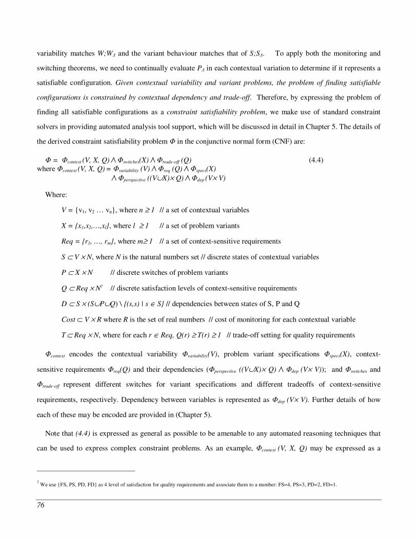
76
variability matches W;W and the variant behaviour matches that of S;S. To apply both the monitoring and
switching theorems, we need to continually evaluate P in each contextual variation to determine if it represents a
satisfiable configuration. Given contextual variability and variant problems, the problem of finding satisfiable
configurations is constrained by contextual dependency and trade-off. Therefore, by expressing the problem of
finding all satisfiable configurations as a constraint satisfiability problem, we make use of standard constraint
solvers in providing automated analysis tool support, which will be discussed in detail in Chapter 5. The details of
the derived constraint satisfiability problem in the conjunctive normal form (CNF) are:
= context (V, X, Q) /\ switches(X) /\ trade-off (Q) (4.4) where context (V, X, Q) = variability (V) /\ req (Q) /\ specs(X)
/\ perspective ((V#X)& Q) /\ dep (V& V)
Where:
V = {v1, v2 … vn}, where n ' 1 // a set of contextual variables
X = {x1,x2,…,xl}, where l ' 1 // a set of problem variants
Req = {r1, …, rm}, where m' 1 // a set of context-sensitive requirements
S " V & N, where N is the natural numbers set // discrete states of contextual variables
P " X & N // discrete switches of problem variants
Q " Req & N7 // discrete satisfaction levels of context-sensitive requirements
D " S & (S#P#Q) \ {(s,s) | s ( S} // dependencies between states of S, P and Q
Cost " V & R where R is the set of real numbers // cost of monitoring for each contextual variable
T " Req & N, where for each r ( Req, Q(r) ' T(r) ' 1 // trade-off setting for quality requirements
context encodes the contextual variability variability(V), problem variant specifications specs(X), context-
sensitive requirements req(Q) and their dependencies (perspective ((V#X)& Q) /\ dep (V& V)); and switches and
trade-off represent different switches for variant specifications and different tradeoffs of context-sensitive
requirements, respectively. Dependency between variables is represented as dep (V& V). Further details of how
each of these may be encoded are provided in (Chapter 5).
Note that (4.4) is expressed as general as possible to be amenable to any automated reasoning techniques that
can be used to express complex constraint problems. As an example, context (V, X, Q) may be expressed as a
7 We use {FS, PS, PD, FD} as 4 level of satisfaction for quality requirements and associate them to a number: FS=4, PS=3, PD=2, FD=1.
77
general constraint programming problem, which provides mechanisms for expressing inequalities. Alternatively,
it may be expressed using propositional satisfiability (SAT) problem, which is limited to Boolean expressions. It
is the latter that we have adopted in this thesis in our initialisation of (4.4). This decision is partly dictated by the
‘natural’ evolution of the research in the sense that, having selected the statechart notation for describing context-
aware specifications (the benefits of which will be discussed in Chapter 5), a constraints based modelling that
allows for the (finite) discrete state descriptions to be encoded into a constraint satisfiability problem appears
appropriate. This allows us to derive the components of (4.4) from both problem frames and statechart problem
descriptions. However, by choosing to use Boolean expression, we loose the power of inequality. This appears not
to be a problem in both the mobile and logistics problems, which we used to both validate our approach and to
assess it industrial relevance (in Chapter 6), as the primary physical variable (location) is finitely partitioned in
both application domains. In differentiating between general constraint problem solving and propositional
constraint solving, we follow the distinction made by (Bordeaux et al., 2005).
4.3.2 Proofs for our Monitoring and Switching Theorems
Considering (4.4) as a Boolean Constraint Satisfiability problem which provides us with a means to derive
satisfiable configurations given a trade-off value, we now express and prove the two theorems as:
Theorem 1’ (Monitoring condition) Given a trade-off tradeoff constrained by context in (4.4), a contextual variable
VAR needs to be monitored if and only if there is a value VAL such that (VAR==VAL) ^ context is satisfiable and
(VAR==VAL) ^ context ^ tradeoff is unsatisfiable.
Proof. (If) Suppose VAR==VAL ^ context ^ tradeoff_ is unsatisfiable and VAR==VAL ^ context is satisfiable, then
VAR=VAL is one possible context under which !tradeoff holds. Therefore one must monitor VAR to avoid
invalidation of context-sensitive requirements.
(Only if) Suppose one has monitored the value of VAR. Then if VAR==VAL is monitored, one knows by the
domain knowledge, VAR==VAL satisfies the context constraints, therefore (VAR==VAL) ^ context. Furthermore,
if VAR==VAL is found invalidating the trade-offs, then (VAR==VAL) ^ context ^ tradeoff is not satisfiable.
Q.E.D.
For brevity, we use VariableValue to represent a proposition that binds a variable to a value: Variable =
=Value. A bound variable is a variable with an assumed or assigned value in a given context.
78
Corollary 1. (Invariant variables) Under all possible contexts, if the binding proposition VAR==VAL always
holds, we do not need to monitor VAR.
Corollary 2. (Invariant context-sensitive requirements) Under all possible contexts, if no matter what value the
variable VAR is bound, the trade-offs of context-sensitive requirements are always satisfied at the same level, we
do not need to monitor VAR.
These corollaries give heuristics that help us avoid monitoring certain variables. Note the second heuristic is
dependent on the trade-offs setting of context-sensitive requirements. The corollaries are sufficient for assessing
the satisfaction of the equivalency criteria defined in theorem 1’. In the case of the first corollary, if the domain
of VAR only consist of VAL, then either both (VAR==VAL) ^ context and (VAR==VAL) ^ context ^ tradeoff are
satisfiable in all contexts or (VAR==VAL) ^ context is satisfiable and but (VAR==VAL) ^ context ^ tradeoff is not
satisfiable. In the latter’s case, this suggest that VAL be monitored. However, since the value of VAR is known to
always be VAL, then no additional information could be provided by further monitoring. Similarly, if for every
VAL taken from the domain of VAR is such that (VAR==VAL) ^ context ^ tradeoff is always satisfied, then the
condition that (VAR==VAL) ^ context be satisfiable and (VAR==VAL) ^ context ^ tradeoff not satisfiable defined
by theorem 1’ can never be met. Hence, VAR would never be monitored accordingly.
Theorem 2’ (Switching condition) Let monitored be the bindings of currently monitored variables. A binding of a
variant specification ’switches is a valid switch from the original binding if switches if switches ^ context ^
monitored ^ tradeoff is unsatisfiable and ’switches ^ context ^ monitored ^ tradeoff is satisfiable.
Proof. If switches ^ context ^ monitored ^ tradeoff is unsatisfiable and ’switches ^ context ^ monitored ^ tradeoff is
satisfiable, and monitored holds, then one has to switch according to trade-offs. Q.E.D.
The consequences of these two theorems are that, given variant specifications (from variant problems) and
knowledge about the contextual dependency on monitoring and switching (Section 4.2), we are able to encode a
constraint satisfiability formula, which enables us to employ the services of a standard SAT-Solver in deriving
satisfiable configurations.
It is important to note that, the use of SAT-Solvers in generating the satisfiable configurations does not in itself
guarantee that the conditions of the monitoring and switching theorems will be met. However, wrapping the
SAT-Solver in our own tool, which we have supported with several algorithms, compliance with the two

79
theorems is enforced at execution time. The development of our tool and its supporting algorithms is the focus of
Chapter 5.
4.4 A Comparative Study
The focus in this section is to highlight the usefulness of problem-oriented analysis of monitoring and
switching activities for context-awareness using the meeting scheduler example problem. In doing so, we again
compare our approach, presented in this section, to that of (Feather et al., 1998), building on the similar
comparison carried out in Section 3.6 on problem classification.
While both Feather et al’s approach and ours explicitly consider the issue of monitorability, their approach
provides no mechanism for replacing variables that cannot be monitored with monitorable ones and for
establishing traceability between the two variables involved. Our use of validation and transformation problems
enables us to provide such a mechanism as illustrated in Section 4.1. Also, while their approach recognises the
need to consider efficiency in switching as evident in:
“In general, systems adaptation should not take place after a single assertion violation by some specific agent
instance; a deviation can be accidental and / or occasional. Moreover, too prompt adaptations could encourage
human agents to deviate too easily”.
Feather et al’s approach does not make a similar recognition in their monitoring problems. Therefore, efficiency
in monitoring is not addressed.
In comparing the treatment of switchability by Feather et al and our approach, recall the distinction made
between deployment-time and run-time switching in Section 2.1.8. In the case of the former, switching is possible
during application start-time and the application cannot be interrupted while execution is underway. In the case of
the latter, switching is possible both during start and execution times. A truly context-aware application must be
capable of carrying out both form of switching. Feather et al’s treatment of application switching only addresses
switching at start-time. Hence, the analysis of the difficult problem of switching during execution is missing. In
illustrating the usefulness of addressing this form of switching, consider the meeting scheduler problem shown in
Figure 12. Consider further a switching problem between Achieve[ConstraintsRequested] and
Achieve[AgendaAccess] in meeting the higher level goal Achieve[ParcipantConstraintsKnown]. To achieve
the higher goal using Achieve[ConstraintsRequested], the requirements is achieved only when the participants

80
have responded by providing the details of their availability. Similarly, the goal is achieved using
Achieve[AgendaAccess] only when an agenda is available and provide the required participant’s availability
details. An execution time switching in this scenario will be a situation in which the application sends a requests
using SendConstraintsRequest but while waiting for a response, the agenda of the participants becomes available
for access. In such a situation, two actions could be taken: (a) recall the message if the participants has not yet
read the message and use Achieve[AgendaAccess] to retrieve the participant’s agenda; (b) ignore the message
or send a message informing the participants not to respond if the message has been read but a response has not
been received and use Achieve[AgendaAccess] to obtain the agenda. In analysing the problem of switching
during execution explicitly, we address the residual effect of the previously used variant behaviour by bringing to
light the need to make a decision about possible alternative actions. Recall that, addressing this form of switching
also refines the set of candidate variables to be monitored by the addition of the need to monitor the status of the
send message to know if it is read or not. This is analogous to the addition of the encryption status variable in the
mobile application problem in Section 4.2.
Although Feather et al recognise the need to address efficiency in switching their recommendation to use
thresholds to determine the number of assertion violations before triggering adaptation response is problematic in
many ways. For instance, it is difficulty to carry out the diagnostics needed to determine violations that are
accidental apart from those that are deliberate. Our use of trade-off analysis to allow for variation in the
satisfaction level of requirements without triggering switching in all cases is relatively more practical in our
opinion. Furthermore, in using constraints satisfiability problems which captures not only the trade-off but
contextual dependencies constraining when switching is permissible is more holistic as it takes into account
contextual constraints in deriving the satisfiable configurations. This will not be possible using thresholds as
recommended by Feather et al.

81
4.5 Chapter Summary
In this chapter, we have presented our problem-oriented approach for analysing the requirements for
monitoring and switching activities aiming to meet the conditions in Table 7. We have provided a means for
analysing the monitorability of elicited candidate variables and for replacing those for which direct monitoring is
not possible using transformation problems (Section 4.1). Similarly, we have provided a means for analysing the
switchability between given pair of variant problems and in analysing the difficult problem of Run-time switching
(Section 4.2). In addressing the question of when to carry out monitoring and switching, to both ensure continual
requirements satisfaction and efficiency in monitoring and switching activities, we have presented a
characterisation of concepts for refining context, which we used to formulate and proved two theorems for
monitoring and switching. This enabled us to carry tool assisted analysis of monitoring and switching activities,
which is the focus of Chapter 5. The benefits of formal and tool assisted analysis includes: (a) automatic
identification of variables, from the candidate variable set, that must be monitored in each context; (b) the
avoidance of monitoring all variables all the time; and (c) a mechanism to initialise the monitored variables
according to their assigned weights (Section 5.1). In the case of switching, the benefits include: (a) ability to
explicitly consider the constraints of the context in specifying the overall switching behaviour, which is taken into
consideration in setting the requirements’ trade-off; and (b) the use of tradeoffs between context-sensitive
requirements to minimise the overall switching behaviour while ensuring that the requirements are continually
being satisfied.

82
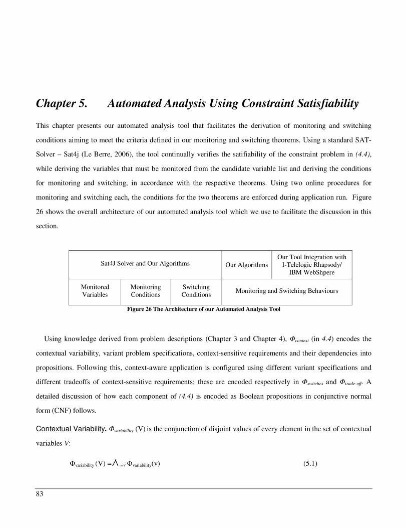
83
Chapter 5. Automated Analysis Using Constraint Satisfiability
This chapter presents our automated analysis tool that facilitates the derivation of monitoring and switching
conditions aiming to meet the criteria defined in our monitoring and switching theorems. Using a standard SAT-
Solver – Sat4j (Le Berre, 2006), the tool continually verifies the satifiability of the constraint problem in (4.4),
while deriving the variables that must be monitored from the candidate variable list and deriving the conditions
for monitoring and switching, in accordance with the respective theorems. Using two online procedures for
monitoring and switching each, the conditions for the two theorems are enforced during application run. Figure
26 shows the overall architecture of our automated analysis tool which we use to facilitate the discussion in this
section.
Sat4J Solver and Our Algorithms
Our Algorithms Our Tool Integration with
I-Telelogic Rhapsody/ IBM WebShpere
Monitored Variables
Monitoring Conditions
Switching Conditions
Monitoring and Switching Behaviours
Figure 26 The Architecture of our Automated Analysis Tool
Using knowledge derived from problem descriptions (Chapter 3 and Chapter 4), context (in 4.4) encodes the
contextual variability, variant problem specifications, context-sensitive requirements and their dependencies into
propositions. Following this, context-aware application is configured using different variant specifications and
different tradeoffs of context-sensitive requirements; these are encoded respectively in switches and trade-off. A
detailed discussion of how each component of (4.4) is encoded as Boolean propositions in conjunctive normal
form (CNF) follows.
Contextual Variability. variability (V) is the conjunction of disjoint values of every element in the set of contextual
variables V:
variability (V) = /\ v(V variability(v) (5.1)
84
We can encode variability for individual contextual variable v using domain properties. This corresponds to the
definition of the domain set from which a variable can take values as discussed in Section 3.2 (i.e., discretisation).
Using our running example, a variable listener can be either authorised or unauthorised but not both, written in
CNF as follows:
variability(Listener) =
(ListenerAuthorised ) ListenerUnauthorised) /\
(!ListenerAuthorised ) !ListenerUnauthorised)
Other variables can be encoded similarly.
Context Sensitive requirements. reqs(Q) is the conjunction of rules that express different satisfaction levels of
each element in the set of context-sensitive requirements Q:
req (Q) = /\ q(Q req(q) (5.2)
In our running example, Q = {security, performance}, both elements have four disjoint levels of satisfaction8
and can only take one value at a time. We can encode reqs (performance) in CNF as follows:
performance = (PerfFS ) PerfPS ) PerfPD ) PerfFD) /\ (!PerfFS ) !PerfPS) /\ (!PerfFS ) !PerfPD) /\
(!PerfFS) !PerfFD) /\ (!PerfPD) !PerfFD)/\ (!PerfPD ) !PerfPS) /\ (!PerfPS )!PerfFD)
One can similarly encode different level of satisfaction for security requirement.
Variant specifications. specs (X) represents disjoint set of variant problems X. Each variant in X addresses a
different perspective.
specs (X) = /\ x(X specs(x) (5.3)
In our running example, specs = z, we can discern two disjoint variants: one with encryption (ON) and the other
without (OFF). Thus, specs(encryption) can be expressed in terms of ON/OFF.
specs (encryption) = (EncryptionON ) EncryptionOFF) /\
(!EncryptionON ) !EncryptionOFF)
8 This is a common approach used in the goal-oriented literature which we have borrowed in illustrating this example
85
Variant specification switches. switches (X) indicates the values of problem variants X that are currently used
in the specifications.
switches (X) = /\ (x,y) ( X switches (x) (5.4)
For example, if encryption is currently ON (i.e., encrypted transmission variant being used), then:
swtiches(encryption) = EncryptionON
Perspectives. perspective ( (V#X)& Q) is the conjunction of rules that express the implications of contextual
variables V and/or variant problems X to the satisfaction of context-sensitive requirements in Q.
Perspective((V#X)& Q) = /\ d((V#X)& Q Perspective(d) (5.5)
As an example for perspective, consider the relationships between different values for the listener and
transmission variables in a security perspective, expressed in CNF as:
Listener_security1 = ! ListenerUnauthorised ) !TransmissionUnsecured ) SecurityFD
Listener_security2 = ! ListenerUnauthorised ) ! TransmissionSecured ) SecurityFS
Listener_security3 = Listener_security2 ^ Listener_security2
This simply states that, when a listener is unauthorised and the transmission is unsecured, the security
requirement is fully denied. It is however fully satisfied when listener is unauthorised and the transmission is
secured.
Trade-off relations. trade-off (Q) encodes the trade-off relations between context-sensitive requirements Q
represented in perspective.
tradeoff (Q) = /\ q(Q tradeoff(q) (5.6)
Each quality requirement trade-off is specified by a certain threshold level of satisfaction. As an example of
Trade-off, consider the trade-off conditions “Security must always be fully satisfied but performance cannot be fully
denied”, expressed as:
trade-off (Security) = SecurityFS trade-off (Performance) = !PerfFD
86
Contextual Dependencies. dep (V& (V#X)) indicates dependencies of values between a contextual variable in V
and a problem variant in V# X.
dep (V& (V#X)) = /\ (x,y) ( V& (V#X) dep (x, y) (5.7)
Here we use implication operator to capture dependency dep (x, y) explicitly as “x implies y” or equivalently “!
x or y” in CNF.
As an example, consider the following dependency: “All listeners are authorised in a secured location”,
expressed as:
dep(LocationSecured, ListenerAuthorised) = LocationSecured implies ListenerAuthorised
This is transformed to its CNF equivalent as:
! LocationSecured ) ListenerAuthorised
Following the discussion of how each component of (4.4) may be encoded into propositions using Boolean
expressions, we are now able to present the details of the underlying algorithms. We begin with a discussion of
how the encoded inputs are fed into the SAT-Solver and how the returned results from it are interpreted. Each
algorithm is discussed under the appropriate section header, focusing on the role it plays in addressing the issues
being considered. However, the full version of the algorithms and the control flow through them can be found in
Appendix A.
Satisfiable contexts (SATcontext): A solution from the SAT-Solver is a list of every atomic proposition (literals
L) of the form either positive L or negative !L. Similarly, input to SAT-Solver is also a list of atomic propositions.
According to our encoding, all these positive literals are in the form of VariableValue. Therefore, to present input
and to receive output from SAT-Solvers, we have implemented an encoder to transform the in (4.4) into an
input to a SAT-Solver, and a decoder to extract context from a solution µ of the SAT-Solver into value
combination of contextual variables.
There are generally two types of SAT-Solvers. The first kind returns any first satisfiable combination of literals
while the second kind exhaustively returns all satisfiable combinations of literals. The latter kind is referred to as
an enumerator. In this thesis, we use a freeware SAT-Solver (Sat4J) which can be used as an enumerator as well.

87
Therefore, in order to find all contexts, we negate the positive literals for every contextual variable and
conjunctively join these negative propositions with to invoke SAT-Solver again. By excluding the solutions
generated one at a time, we can exhaustively find all context solutions satisfying . This repeated call to the SAT-
Solver will not be necessary if an enumerator is used, whenever available. These solutions are stored in a map
SATcontext that contains the bindings of variables to the propositional satisfiability problem.
SATcontextGeneration(V’m, X, S, P, )
1 INPUT
2 V’m" V // an ordered list of subset of V (list of monitorable variables) to be monitored,
3 // same as defined in (4).
4 X = {x1,x2,…,xl}, where l ' 1 // a set of problem variants
5 S " V & N, where N is the natural numbers set // discrete states of contextual variables
6 P " X & N // discrete switches of problem variants
7 OUTPUT: SATcontext
8 BEGIN
9 S() = { } // initialise as an empty set of context variant bindings
10 R8 =
11 WHILE satisfiable (R8) DO
12 S =* v(V’m, 1+ s+ S(v) (v=s) ^ * x(X, 1+ p+ P(x) (x=p) such that S entails
// decode satisfiable result as previously explained
13 S() = S() # { S }
14 R8= R8 $ ! S // remove the current satisfiable result µ from possible future resutls
15 ENDDO
16 SATcontext = S()
17 RETURN SATcontext
18 END
Storing all satisfiable bindings to contextual changes in SATcontext, we avoid calling the SAT-Solver at
execution-time to evaluate contextual changes by simply searching for the existence of a given context’s state in
SATcontext.
88
In the following sections, we continue to extract the relevant portions of our tool and algorithms pertaining to
the discussion of each section. The above algorithm corresponds to Algorithm 7 in Appendix A.
5.1 Monitored Variables
This section presents the algorithms for eliciting monitored variables. Also, presented here are the algorithms
for ranking monitored variable in support of initialisation.
5.1.1 Algorithm for Eliciting Monitored Variables
Given an initial candidate contextual variables, W (v1, v2,…, vn), we select contextual variables that must be
monitored during run-time to assess the satisfaction of by testing for the satisfaction of (4.4) using the condition
defined in the monitoring theorem: (i.e., ( $ v = i) $ (not $ v = j) where i and j represent different values of a
variable v). Therefore, not all contextual variables may be monitored. During problem classification (Chapter 3),
the focus is on the relevance of the variable in determining the satisfaction of the requirement. Therefore, it may
not be apparent to the analyst that this variable need not be monitored as the information it provides can be
derived from other monitored variables (i.e., the impact of contextual dependency is not considered). However,
once the dependency between variables and or context sensitive requirements are encoded in dep, the automated
tool automatically identifies and removes variables that must never be monitored and those that are conditionally
monitored. In the latter’s case, the variables are temporarily removed only when the sufficiency condition dictates
it. The high level pseudo code view of the implementation is presented in ElicitMonitoredVariables, which
corresponds to Algorithm 2 in Appendix A. While invoking the SAT-Solver to check for Monitor_Check = ( $
v = i) $ (not $ v = j) (line 14 in ElicitMonitoredVariables), we elicit a list of monitored variables as Vm which
is returned to the calling algorithm.

89
ElicitMonitoredVariables (V, X, Req, S, P, Q, D, T)
1 INPUT: V, X, Req, S, P, Q, D, T. Where,
2 V = {v1, v2 … vn}, where n ' 1 // a set of contextual variables
3 Req = {r1, …, rm}, where m' 1 // a set of context-sensitive requirements
4 Q " Req & N // discrete satisfaction levels of context-sensitive requirements9
5 D " S & (S#P#Q) \ {(s,s) | s ( S} // dependencies between states of S, P and Q
6 T " Req & N, where for each r ( Req, Q(r) ' T(r) ' 1 // trade-off setting for
//context-sensitive core requirements
7 S, X, P // as previously defined
8 OUTPUT: Vm // list of variables that may be monitored
9 BEGIN
10 Vm = { } // Initialise the set of monitored contextual variables to the empty set
11 = EncodeVariabilityAndDependency (V, X, Req, S, P, Q, D, T) //Algorithm 8
12 FOR EACH v (V DO
13 FOR EACH i, j ([1 .. S(v)] | i % j DO
// construct validation condition using the Monitoring theorem
14 Monitor_Check = ( $ v = i) $ (not $ v = j) // invoke SAT-Solver
15 IF satisfiable(Monitor_Check) THEN
16 Vm = Vm # {v} // add the contextual variable to be monitored:
17 BREAK
18 ENDIF
19 ENDDO
20 ENDDO
21 RETURN Vm
22 END
9 We use {FS, PS, PD, FD} as 4 level of satisfaction for quality requirements and associate them to a number: FS=4, PS=3, PD=2, FD=1.
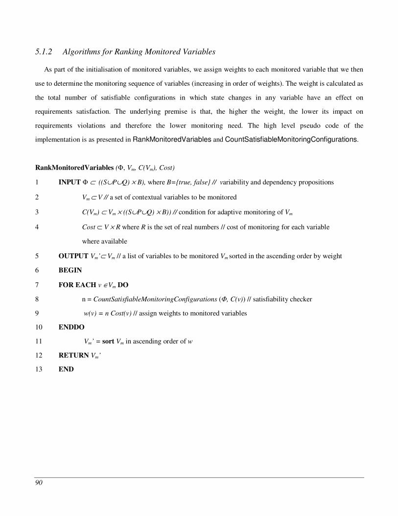
90
5.1.2 Algorithms for Ranking Monitored Variables
As part of the initialisation of monitored variables, we assign weights to each monitored variable that we then
use to determine the monitoring sequence of variables (increasing in order of weights). The weight is calculated as
the total number of satisfiable configurations in which state changes in any variable have an effect on
requirements satisfaction. The underlying premise is that, the higher the weight, the lower its impact on
requirements violations and therefore the lower monitoring need. The high level pseudo code of the
implementation is as presented in RankMonitoredVariables and CountSatisfiableMonitoringConfigurations.
RankMonitoredVariables (, Vm, C(Vm), Cost)
1 INPUT " ((S#P#Q) & B), where B={true, false} // variability and dependency propositions
2 Vm " V // a set of contextual variables to be monitored
3 C(Vm) " Vm & ((S#P#Q) & B)) // condition for adaptive monitoring of Vm
4 Cost " V & R where R is the set of real numbers // cost of monitoring for each variable
where available
5 OUTPUT Vm’" Vm // a list of variables to be monitored Vm sorted in the ascending order by weight
6 BEGIN
7 FOR EACH v (Vm DO
8 n = CountSatisfiableMonitoringConfigurations (, C(v)) // satisfiability checker
9 w(v) = n Cost(v) // assign weights to monitored variables
10 ENDDO
11 Vm’ = sort Vm in ascending order of w
12 RETURN Vm’
13 END
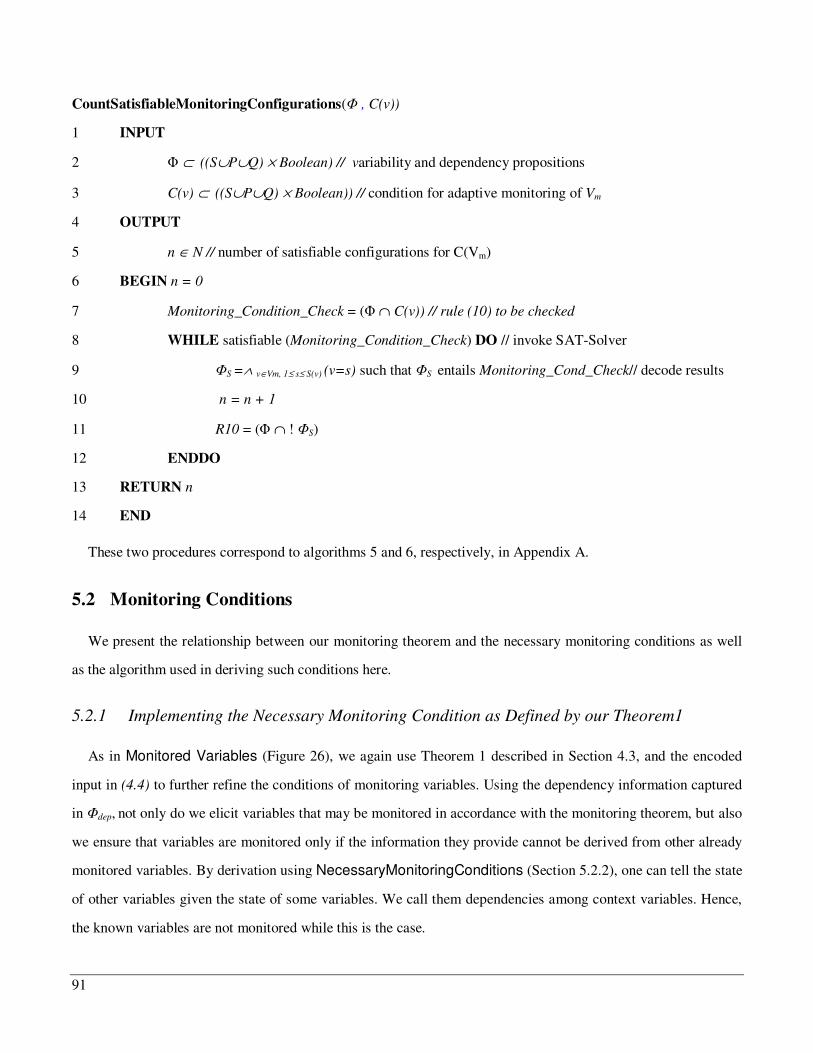
91
CountSatisfiableMonitoringConfigurations( , C(v))
1 INPUT
2 " ((S#P#Q) & Boolean) // variability and dependency propositions
3 C(v) " ((S#P#Q) & Boolean)) // condition for adaptive monitoring of Vm
4 OUTPUT
5 n ( N // number of satisfiable configurations for C(Vm)
6 BEGIN n = 0
7 Monitoring_Condition_Check = ( $ C(v)) // rule (10) to be checked
8 WHILE satisfiable (Monitoring_Condition_Check) DO // invoke SAT-Solver
9 S =* v(Vm, 1+ s+ S(v) (v=s) such that S entails Monitoring_Cond_Check// decode results
10 n = n + 1
11 R10 = ( $ ! S)
12 ENDDO
13 RETURN n
14 END
These two procedures correspond to algorithms 5 and 6, respectively, in Appendix A.
5.2 Monitoring Conditions
We present the relationship between our monitoring theorem and the necessary monitoring conditions as well
as the algorithm used in deriving such conditions here.
5.2.1 Implementing the Necessary Monitoring Condition as Defined by our Theorem1
As in Monitored Variables (Figure 26), we again use Theorem 1 described in Section 4.3, and the encoded
input in (4.4) to further refine the conditions of monitoring variables. Using the dependency information captured
in dep, not only do we elicit variables that may be monitored in accordance with the monitoring theorem, but also
we ensure that variables are monitored only if the information they provide cannot be derived from other already
monitored variables. By derivation using NecessaryMonitoringConditions (Section 5.2.2), one can tell the state
of other variables given the state of some variables. We call them dependencies among context variables. Hence,
the known variables are not monitored while this is the case.

92
5.2.2 Algorithm for Deriving Necessary Monitoring Conditions
In deriving the necessary monitoring conditions, we check for C(vj) = C(vj) * (vi%k)(line 9) in
NecessaryMonitoringConditions below. This effectively ensures that variable vj would be monitored as long as
vi is not currently bound to k. Similarly, given the state of some variables, one can tell that changes in other
variables have no impact in the satisfaction of a requirement being considered. We call them redundancies among
context variables. All redundant variables are not monitored. Again, this condition is checked in C(vj) = C(vj) *
(vi%k ) r %q). In this case, the monitoring condition for vj states that it should be monitored only either vi is not
currently bound to k or the currently assessed requirement r is not bound to q.
NecessaryMonitoringConditions (Vm, DC , D, Req, Q , S)
1 INPUT Vm " V // a set of contextual variables to be monitored
2 DC " S & (S \ {(s,s) | s ( S}) // Dependency among contextual variables
3 D, Req, Q, S // same as previously defined
4 OUTPUT C(Vm) " Vm & ((S#P#Q) & B)) // conditions for necessary monitoring of Vm
5 BEGIN C(vi) = true for every vi ( Vm // Initialise
6 FOR EACH i, j ([1 .. |Vm|] | i % j DO
7 FOR EACH k ( S(vi) DO
8 IF | { m | m ( S(vj) * (k, m) ( DC } | = 1 THEN
// Condition set by the Theorem 1’ and (4)
9 C(vj) = C(vj) * (vi%k)
10 ELSE IF (k, q) ( D where r ( Req * (r , q ) ( Q THEN
// Condition set by the Theorem 1’ and (4)
11 C(vj) = C(vj) * (vi%k ) r %q )
12 ENDIF
13 ENDDO
14 ENDDO
15 RETURN C(Vm)
16 END
This procedure corresponds to algorithm 4 in Appendix A.
93
5.3 Switching Conditions
We present the relationship between our switching theorem and the necessary switching conditions as well as
the algorithm used in deriving such conditions here.
5.3.1 Implementing the Necessary Switching Condition as Defined by our Theorem 2
As in Derive Monitoring Behaviour, we use theorem 2 described in Section 4.3, and the encoded input in
(4.4) to derive the conditions for switching variant specifications. Using the dependency information captured in
dep and the trade-off specification in trade-off, we only switch behaviour when a change in context results in the
violation of requirements as specified in trade-off while acknowledging the constraints of the context in dep. This
means that not all changes in reqs results in switching behaviour as such changes may fall within the bounds of
trade-off. In DeriveMonitoringSwitchingConditionsAndSimulatingProcedures, C(x=p) = { (s1, ..., st) | (*i=1..t vi=si) *
* (x=p)} (line 12) elicits satisfiable bindings between variants and context, where represents equation (4.4).
Algorithms 2, 4, 5, 7 and 10 (See appendix A) as used in
DeriveMonitoringSwitchingConditionsAndSimulatingProcedures matches those in Appendix A.
5.3.2 Algorithm for Deriving Necessary Switching Conditions
DeriveMonitoringSwitchingConditionsAndSimulatingProcedures (V, X, Req, S, P, Q, D, Cost, T)
1 INPUT
2 V, X, Req, S, P, Q, D, Cost, T // as previously defined
3 BEGIN
4 S(Vm) = { S(v) | v ( Vm } // aggregate all states of monitored contextual variables
5 DC = { (s1, s2) |
(s1, s2) ( D * s1, s2 ( S(Vm) } // dependency among contextual variables
6 Vm = ElicitMonitoredVariables (V, X, Req, S, P, Q, D, T) // Algorithm 2
7 = RemoveRedundantRules(, C(Vm)) // Algorithm 3
8 C(Vm) = NecessaryMonitoringConditions(Vm, DC, D, Req, Q, S) // Algorithm 4
9 V’m = RankMonitoredVariables(, Vm, C(Vm), Cost) // Algorithm 5
10 t = | V’m | // the number of monitored context variables
94
// starts the implementation of the conditions in Theorem 2’:
11 FOR EACH x ( X and p([1.. P(x)] DO //deriving switching conditions
12 C(x=p) = { (s1, ..., st) | (*i=1..t vi=si) * * (x=p)}
13 ENDDO
//ends the implementation of the conditions in Theorem2’
14 SATcontext = SATcontextGeneration(V’m, X, S, P, ) // SATcontextGeneration
15 SimulateMonitoringSwitchingProcedure(Vm’, X, SATcontext) // Algorithm 10
16 END
5.4 Monitoring and Switching Behaviours Simulation
The presentation here is focused on how Simulate Monitoring and Switching Behaviours is implemented
using two procedures, which we use to simulate monitoring and switching activities in support of verification of
our two theorems.
In order to avoid re-computing the satisfiability of context ^ monitored ^ tradeoff which is more restricted than
context ^ tradeoff in (4.4), we can filter out the already monitored ones, where monitored holds from the satisfied
solutions to (4.4). As a result, we create a look up table SATcontext for each monitored context monitored^ context to
tell which contextual variables in Vm need to be continually monitored.
5.4.1 Algorithm for Simulating Monitoring Behaviour
A high level description of the monitoring behaviour simulation procedures is as given below:
SimulateMonitoringSwitchingProcedure (Vm, X, SATcontext)
1 INPUT
2 Vm // a list of all monitored contextual variables
3 X // a list of all variant problems
4 SATcontext // same as previously defined
95
5 BEGIN
6 switches = /\ x(X x=1
7 WHILE (true) DO
8 currentSATContext = SATcontext [random(|SATcontext|)] // a random context is selected
9 // monitored is values of currently monitored part of the context
10 // context is values of contextual variables and contextual dependency information
11 // switches is the current values of switches
12 // tradeoff is the current values of the trade-off setting
13 Extract monitored, context, switches and tradeoff from currentSATContext
14 FOR EACH VAR IN Vm DO
15 IF there is a VAL such that:
16 currentSATContext [VAR==VAL ^ context ^ monitored ^ switches] AND
17 ! currentSATContext [VAR==VAL ^context ^ monitored ^ switches ^ tradeoff] THEN
// Let VAR=VAL be monitored for changes in VAR
18 monitored = monitored /\ VAR==VAL
19 ENDIF
20 END FOR
21 SwitchingProcedure (monitored, context, switches, tradeoff, SATcontext) // Algorithm 11
22 END WHILE
23 END
5.4.2 Algorithm for Simulating Switching Behaviour
A high level description of the switching behaviour simulation procedures is as given below:
SwitchingProcedure (monitored, context, switches, tradeoff, SATcontext)
1 INPUT monitored, context, switches, tradeoff //same as defined in Algorithm10
2 SATcontext // same as defined in Algorithm 8
3 OUTPUT switches // satisfable set of switches

96
4 BEGIN
5 NeedSwitch = SATcontext [monitored ^ context ^ switches^ tradeoffs]
6 IF ! NeedSwitch THEN
7 RETURN switches // no need to switch
8 ELSE
9 BestTradeoff = tradeoff
10 BestSwitches = switches
11 END IF
12 FOR EACH binding of switches ’switches DO
13 IF (’tradeoff implies BestTradeoff AND
14 ! SATcontext[switches ^ monitored ^ context ^ ’tradeoff] AND
15 SATcontext[’switches ^ monitored ^ context ^ ’tradeoff]) THEN
16 BestTradeoff = ’tradeoff
17 BestSwitches = ’switches
18 BREAK // Any new satisfying switches is fine
19 END IF
20 END FOR
21 RETURN BestSwitches
22 END
Using the two procedures above, we simulate monitoring and switching behaviours corresponding to Our
Algorithms (only) component in Figure 26 the output of which is saved in a file. Subsequently, we use the saved
output to control context-aware problem descriptions in statechart and process model descriptions. The latter
activity corresponds to Telelogic Rhapsody/IBM WebSphere Integration with our Tool component. The use
of the derived monitoring and switching conditions to construct dynamic problem descriptions in statechart or
process models enables us to further analyse temporal concerns such as the reactions of monitors to contextual
changes. Rhapsody provides a mechanism to link statechart models to standard Java applications, a facility we
have used to integrate our tool into Rhapsody. We simulate contextual changes in the Java applications, but show
its effect in terms of the monitor and switcher behaviours and their effect on variant behaviours, which we
97
modelled as parallel state machines. This allows us to manage scalability. The alternative would have been to
model the variant behaviours sequentially, which is subsequently (parallel) composed with the monitoring and
switching behaviours. This is the approached used in our publication in (Salifu et al., 2007b, Salifu et al., 2007a).
The problem with this (latter) alternative is that, it does not scale well as the number of transitional connections
quickly explodes as the number of variants increases. By modelling variant specifications as XOR sub-states
embedded in parallel state machines, among which only one represents the current variant where the other
represent flags of the other mutually exclusive variants, we eliminate the transitions explosion problem. In
essence, by controlling each variant through a corresponding event that transits from flag states to the state of the
variant, we can stack up any number of variant specifications. Therefore, the number of variables and their states
has no impact on the statechart model where they are hidden. Also, by explicitly showing the validation
specification as a state machine, we can continually validate the model even when new variants are being added
by executing a recompiled simulation model. Similarly, IBM WebSphere provides a mechanism for linking
process models to data repositories (i.e., data files).
Having reviewed our tool assisted approach to deriving monitoring and switching conditions, we now have all
the components needed to construct context-aware specifications. From the equations presented in this thesis thus
far, we can express context-awareness as:
W;WM;Ws;S;S;SM;Ss, Sca Rca (5.8)
where W;WM;Ws;S;S;SM;Ss in (5.8) together represent Wca and Rca entails R, RM and RS.
Therefore, using the derived monitoring and switching conditions, which form part of Rca, we parallel compose
variants, monitoring and switching specifications to produce the required context-aware behaviour. We describe
context aware problems in accordance with (5.8) using statechart or process models. For an example see the
problem description in Figure 43, in which the two online procedures are implemented in I-Telelogic Rhapsody to
enforce the criteria defined in the monitoring and switching theorems.
A detailed conceptual model relating all the key concepts used in this thesis can be found in Appendix C.
98
5.5 Chapter Summary
We have presented our automated analysis tool that facilitates the derivation of monitoring and switching
conditions aiming to meet the criteria defined in our monitoring and switching theorems. Using a standard SAT-
Solver (Sat4j), which we wrapped in our several algorithms, the tool continually verifies the satisfiability of the
constraint problem in (4.4), while deriving the variables that must be monitored from the candidate variable list
and in deriving the conditions for monitoring and switching. We have also presented details of our underlying
algorithms of our analysis tool, the output of which is the required conditions for monitoring and switching
activities in support of context-awareness.
Using the derived monitoring and switching conditions, which effectively form part of the context-aware
specification, we parallel compose variants, monitoring and switching specifications to produce the required
context-aware behaviour. By parallel compose we mean, variant specifications are modelled as XOR sub-states
embedded in parallel state machines, among which only one represents the current variant. The benefit is that, the
number of variables and their states has no impact on the statechart, which enables our context-aware
specifications to scale well in the statechart descriptions.
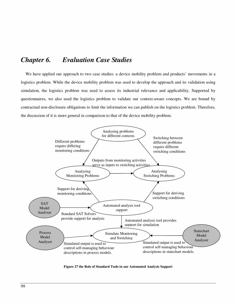
99
Chapter 6. Evaluation Case Studies
We have applied our approach to two case studies: a device mobility problem and products’ movements in a
logistics problem. While the device mobility problem was used to develop the approach and its validation using
simulation, the logistics problem was used to assess its industrial relevance and applicability. Supported by
questionnaires, we also used the logistics problem to validate our context-aware concepts. We are bound by
contractual non-disclosure obligations to limit the information we can publish on the logistics problem. Therefore,
the discussion of it is more general in comparison to that of the device mobility problem.
Figure 27 the Role of Standard Tools in our Automated Analysis Support
Analysing problems for different contexts
Analysing Monitoring Problems
Analysing Switching Problems
Different problems require differing monitoring conditions
Switching between different problems require different switching conditions
Outputs from monitoring activities serve as inputs to switching activities
Automated analysis tool support
Support for deriving monitoring conditions Support for deriving
switching conditions
SAT Model
Analyser
Process Model
Analyser
Statechart Model
Analyser
Simulate Monitoring and Switching
Automated analysis tool provides support for simulation
Standard SAT Solvers provide support for analysis
Simulated output is used to control self-managing behaviour descriptions in process models.
Simulated output is used to control self-managing behaviour descriptions in statechart models.
100
Recall that we first introduced the mobile device problem in Chapter 3, which we subsequently used
throughout the thesis, thus far, to facilitate the introduction of concepts and in illustrating their usefulness in
analysing context-awareness problems. We now consolidate the various scattered illustrations of the mobile
device problem in Section 6.1 and show the use of standard tools as part of our automated analysis support (see
Figure 27). The logistics problem is similarly analysed in Section 6.1.4 to show the industrial relevance of our
approach. The use of these two case studies supports the adopted research methodology: a hybrid of qualitative
and quantitative research methodologies. In Figure 27, the highlighted oval shapes represent the standard tools
which we have found useful in analysing context-awareness problems and in-cooperated into our automated
analysis tool.
It is worth noting that, the primary changeable property in the two case studies is physical location. In the
mobile application, it is the location in which the device is used. This physical property is commonly partitioned
using latitude and longitude coordinates. Fixed landmarks such as historic building could also be used as the basis
for partitioning location. Various location detection technologies such as Geographical Positioning System (GPS)
and Assisted Geographical Positioning System (A-GPS) are commonly used to monitor location changes when
mobile devices are being used.
6.1 Approach Application (Mobile Device Problem)
The mobile device application problem came to light during an exploratory investigation into the use of
variability techniques to design product-families (Salifu et al., 2006). We studied eight models of Nokia mobile
phones (1100, 3310, 6610, 7250, 6800, 6600, 3650 and 9500). The Nokia phone product-family was chosen for
the pilot study due its wide range of phones; between 500-600 million Nokia phones were estimated to be used
globally (Bosch, 2005). This provides a rich source of varied data covering a range of variability sources suitable
for the areas we investigated.
We found, mainly five sources of variability in the study, ranging from physical handset categories to operating
platforms. They are largely grouped into two categories based on the operating platform (solution-oriented) and

101
applications (problem-oriented), which is requirements/problem-oriented10. We now briefly discuss each of the
categories, starting with the problem-oriented categorisation followed by the solution-oriented one.
Nokia classifies applications domains into four types of problem areas. These are, Mobile, Enterprise, Home
and Internet domains11, each of which is briefly discussed next.
Mobile Domain: The Mobile domain provides person-to-person communication (i.e., voice) and data transport
services such as picture transmission. The main concerns are: mobility management, authentication, charging, and
other value adding functionalities that are supported by the cellular network infrastructure. Its primary
requirement is to provide richer communications through various media; voice, text images, streaming video and
combinations thereof.
Enterprise domain: In the Enterprise domain, the primary user – usually an employee - connects to IT services,
business applications, other employees, and customers. Employees need various types of enterprise applications,
like corporate Personal Information Management (PIM) and communication services (such as instant messaging
and email), databases, business services, and collaboration tools, as well as Internet services. Access to these
services can take place in various environments - e.g. at home, at the office, or at the airport - using various
devices and access channels, such as wireless networks, Wireless Local Area Networks (WLANs), and fixed
broadband access.
Home domain: The Home domain includes communications, collaboration such as groups of persons working on
a shared project, and content sharing within the physical boundaries of the home as well as within the “extended
home” (e.g., using intranet or the Internet). Family- or home-related activities happening outside the home are
considered part of the extended home. The extended home environment is becoming more significant as
consumers want to access information and entertainment, view and share self-created content, and exchange
messages with family members regardless of time or place.
Internet Domain: In the Internet domain, all the services are provided by a multitude of companies,
organizations and even individual users. The evident driving force in the Internet domain is the increasing
consumption of media in addition to traditional e-mail, WWW services and instant messaging. One is able to
10 http://europe.nokia.com/nokia/0,62626,00.html 11
The term ‘domain’ used here refers to Nokia’s classification of application areas.

102
publish his/her own content and interact with friends and communities regardless of time, place or connection
type.
Considering the above classification, Nokia observed that it was inadequate at capturing the variability of the
problem space. This is because, within a given application domain such as the Home domain, different users have
different purchasing capability and needs. To address this, Nokia proposed a market-oriented classification that
cuts across the four application domains. That is, different segments could co-exist within an application domain.
For example, Nokia 7250 was classified as ‘Fashion’ while 6800 was classified as ‘Enterprise’ segments but both
phones provide functions associated with the ‘enterprise domain’. Five segments have been proposed, which we
briefly discuss next.
Entry level: This refers to phone with basic features such as the ability to make a phone call and to send a text
message. This category of phones also has limited gaming and basic user interface features. Examples of Nokia
entry phones are 3310 and 1100.
High End: This category is made up of phones of advanced features such as the ability to run third party
application such as Microsoft Office applications and advanced user interface features such as voice messaging.
Examples of phones of this category are 6600 and 6610.
Enterprise: This is primarily targeted at the corporate world aimed at providing continual business process while
on the move. Therefore, in addition to having the ability to run third party application such as MS Office
applications, they are also equipped to secure their communication channels with facilities such as the use of
virtual private networks (VPN). Examples of phones in this category are 6800 and 9500.
Fashion: The features that uniquely identify this category are largely user interface driven designed to appeal to
users who pay special attention to the external observable features of a phone such as cover case colour and
keypad layout. Examples of phone in this category are Nokia 3650 and 7250.
Rough: This is designed for people who are mostly outdoors or put phones under physical strain. Most of the
specialised features are hardware based and cover areas such as shock and water-resistant covers and scratch-
proof display. However software also plays some part in allowing the phone to be used for other services such as
stopwatch and as a camera. An example of this is 5410.
103
Obviously, not all the identified segments such as Fashion present software challenges. Nevertheless, Nokia
needed a design (classification) platform that supports the derivation of products (i.e., phones) by both application
domains and market segmentation. To meet this challenge, Nokia and its partners developed a four platform
classification of its architectures, each of which is discussed next. The four classification corresponds to operating
system platforms S30, S40, S60, and S80 (Nokia, 2005), as shown in Figure 28. Each platform may have several
versions with each version offering different application libraries for system developers (Nokia, 2006), as shown
in Figure 30. Also, different platform versions have additional capability which is achieved using the Javatm 2
platform (the Micro Edition that is specialised for the mobile application environment). Furthermore, the FTP
API row for the S60 platform shows that platform versioning may include the removal of functions not only the
addition of new ones. Each of the four platforms is briefly discussed next.
Series 30: Series 30 is based on Nokia's proprietary Operating System, designed for entry-level Nokia phones.
The platform is optimised for easy-to-use products that target first time users in, for example, new growth
markets. This platform is claimed by Nokia to have a significant memory cost benefit compared to fully featured
platforms, which makes it is highly cost-effective and caters for customers seeking lower price points. Due to
being both affordable and easy-to-use, Series 30 is said to be the ideal platform for enabling millions of first time
users to go mobile and to gain the socio-economic benefits of mobility. Technically,
Series 30 serves best for voice-centric products with simple text and picture messaging functionality - both in
GSM and CDMA markets. Also, this platform is claimed by Nokia to have an intuitive, visually attractive user
interface, with graphics enhancements and selected value-adding features like built-in games.
Series 40: Series 40 is based on Nokia's proprietary Operating System developed by a third party - Symbian. It is
claimed by Nokia to be highly configurable and flexible software platform that enables a wide variety of different
user interface styles and displays, product concepts and feature configurations. This enables the provision of
distinctive, innovative products for different product categories, target users, and markets. For example, the Series
40 platform allows for the customization of devices for Nokia’s different operator customers with distinctive
operator branded soft-keys, operator logos and ring tones, colour schemes and wallpapers, wake up graphics,
bookmark & link delegates, and data settings. Technically, Java, XHTML Browser, and Multimedia Messaging
Service (MMS) are used as the mechanism to open the platform to the developers' community, i.e., third party
developers such as game developers.
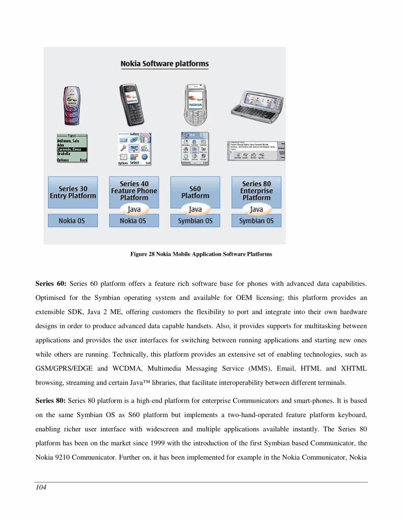
104
Figure 28 Nokia Mobile Application Software Platforms
Series 60: Series 60 platform offers a feature rich software base for phones with advanced data capabilities.
Optimised for the Symbian operating system and available for OEM licensing; this platform provides an
extensible SDK, Java 2 ME, offering customers the flexibility to port and integrate into their own hardware
designs in order to produce advanced data capable handsets. Also, it provides supports for multitasking between
applications and provides the user interfaces for switching between running applications and starting new ones
while others are running. Technically, this platform provides an extensive set of enabling technologies, such as
GSM/GPRS/EDGE and WCDMA, Multimedia Messaging Service (MMS), Email, HTML and XHTML
browsing, streaming and certain Java™ libraries, that facilitate interoperability between different terminals.
Series 80: Series 80 platform is a high-end platform for enterprise Communicators and smart-phones. It is based
on the same Symbian OS as S60 platform but implements a two-hand-operated feature platform keyboard,
enabling richer user interface with widescreen and multiple applications available instantly. The Series 80
platform has been on the market since 1999 with the introduction of the first Symbian based Communicator, the
Nokia 9210 Communicator. Further on, it has been implemented for example in the Nokia Communicator, Nokia

105
9290 Communicator, Nokia 9500 Communicator and Nokia 9300 smart-phone. This platform has been optimized
for enterprise productivity applications like email, calendar, contacts/phonebook, printing and Microsoft Office™
compatible applications for Word document, spreadsheet, and presentation creation and editing.
From the foregoing discussion, we represent the variability dependency between the classifications using the
FODA (Schobbens et al., 2006) notation as shown in Figure 29. The upper part shows the relation between
platforms and individual phones, which represents a solution-oriented classification. Conversely, the lower part
shows the relation between, the same set of, phones and market segments on one hand and Nokia usage domains
on the other. Notice the apparent use of the mobile usage domain as a base or foundation upon which other usage
domains are built. In other words, every mobile phone must have the capability to meet the functional
requirements of the mobile usage domain, but may additionally be equipped other functionalities.
Figure 29 Requirement Vs. Design Variability Dependency Relations of the Nokia Product-Family

106
Besides having different physical features such as the presence or absence of a digital camera or FM radio, we
observed that similar function across different domains was treated differently. For example, while transmission
between enterprise domain phones could be secured using the SSL/TLS encryption standard, transmission
between home domain phones could not. This brought our attention to the assumptions being made about the
different application domains. In this case, they assume that home domain phone users do not care about the
security or privacy of their data being transmitted. This may not always be the case.
Considering these application domains and segments as partitions of contextual variability, we argue that what
is needed is the ability to meet the same requirements using different techniques in different contexts. Also, as
hardware variability is increasingly moved into software variability as observed in (Maccari and Heie, 2005), it is
our view that this problem will need to be addressed in order to make mobile devices more context-sensitive.
Given that our approach is problem-oriented aiming at achieving adequate problem analysis; we focused on
the Nokia application domain based categorisation in deriving the example mobile application. From the
foregoing discussion in this section, it can be seen that irrespective of the application domain type, the
fundamental problem is that of mobility management of person-to-person voice or data transmission between
locations. For instance, in the case of the (general) mobile domain, the aim is to provide richer communications
through various media; voice, text images, streaming video and combinations thereof. Similarly, the enterprise
domain is aiming at business employees whose main functionalities include connecting to IT services, business
applications, other employees, and customers. In deriving a proof of concept mobile application problem, we limit
the mobility management problem to that of managing the efficiency and security concerns of data transmissions
between mobile devices in varying usage context.
A reduction in the general problem of mobility management was necessary in building our understanding of
this unfamiliar application domain and in solving a manageable size problem given the time constraints of PhD
studies. Nevertheless, the analysis of context-awareness for the device mobility domain has enhanced our
understanding of the dynamic relations between requirements and products variability, which we discussed next.
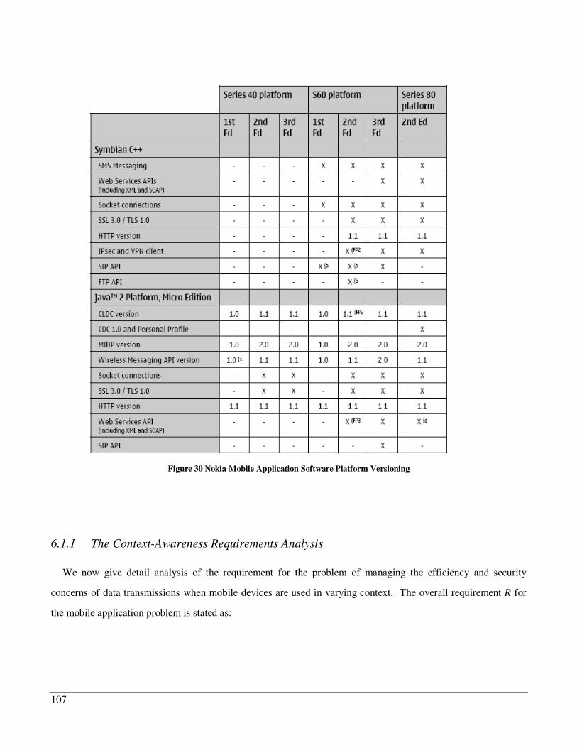
107
Figure 30 Nokia Mobile Application Software Platform Versioning
6.1.1 The Context-Awareness Requirements Analysis
We now give detail analysis of the requirement for the problem of managing the efficiency and security
concerns of data transmissions when mobile devices are used in varying context. The overall requirement R for
the mobile application problem is stated as:
108
A secured and efficient wireless transfer of images from a digital camera to a mobile phone’s storage is
required. All transmissions must be secured while remaining as efficient as possible, in all operating contexts.
Secured transmission refers to the prevention of transmitted data falling into the hands of malicious or
unauthorised persons; while efficiency refers to the minimisation of securing transmission data overheads.
From the foregoing review of the pilot study, we claim that R meets the general requirement of both the Mobile
and Home domains. In the former case, it falls under data transport services, while in the latter it falls under
collaboration and content sharing. Also, while the transmissions between the two mobile devices may involve the
cellular network infrastructure, it need not be the case in all transmissions as other wireless technologies such as
Bluetooth and Wi-Fi may also be used. We argue that while there may be differences in the solution space due to
the differing technologies, the fundamental requirement within the problem space remains the same: Changing the
mechanism of data transmission between the two mobile devices to meet the same requirement under different
contexts. Therefore, we use the term ‘wireless transfer’ generically in analysing the mobile problem.
In order to identify and elicit variables that may be monitored, we begin with a sketch of the context in which
data transmissions take place. Using the above requirement statement, together with the domain knowledge
gained from the pilot study, we elicit the following problem contextual domains:
Wireless transmission medium
External Digital Camera
Mobile Phone Storage
Potential Transmission Listener
We define secured transmission as the prevention of transmitted data falling into the hands of a malicious or
unauthorised transmission listener. Therefore, in contexts where everyone is assumed to be authorised, a secured
transmission is achieved using an unsecured data transmission. Also, the efficiency requirement may suffer in
contexts where data transmissions are secured when everyone is authorised to have access to the data being
transmitted. Hence, the status of Potential Transmission Listeners may be monitored. Therefore, we must
consider it as a problem domain to be analysed for monitorability. Also, note the statement: in all operating
contexts hints there is a need for context-awareness.
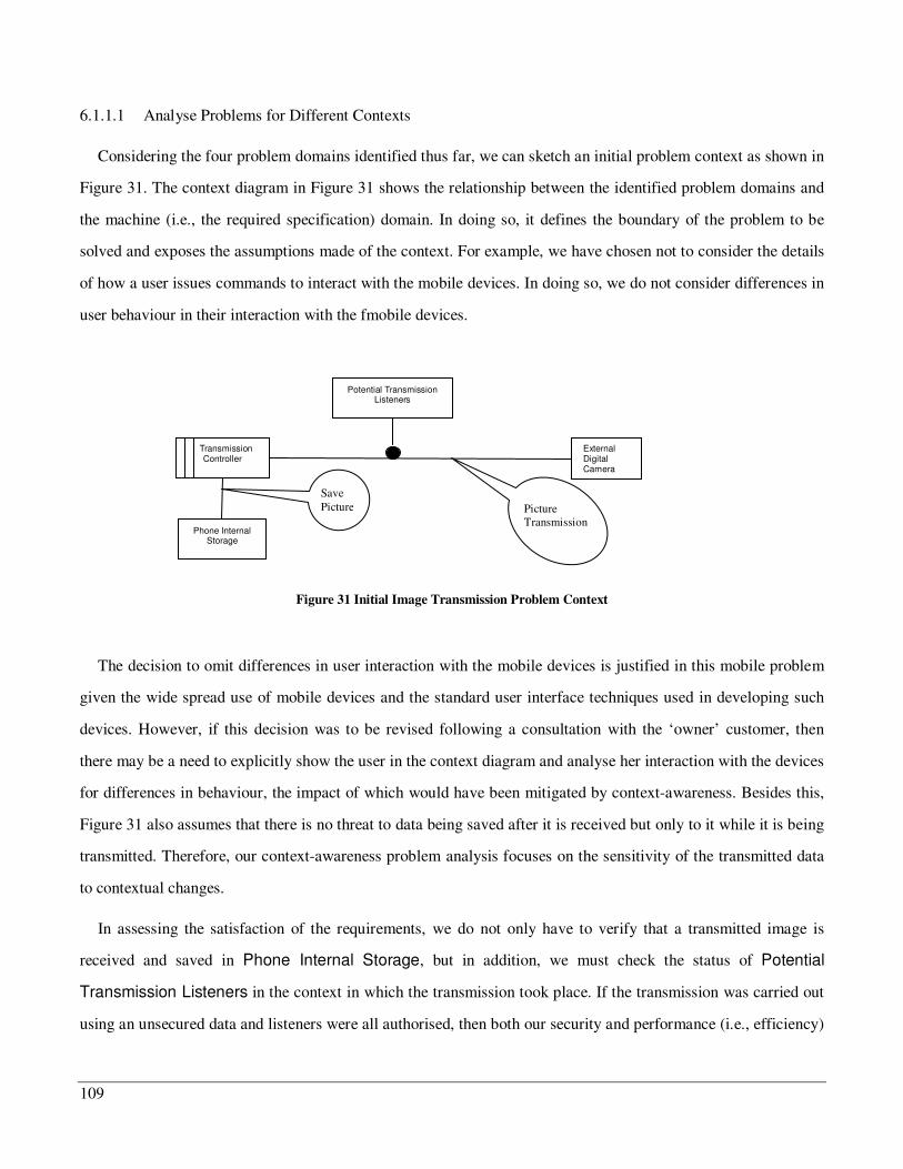
109
6.1.1.1 Analyse Problems for Different Contexts
Considering the four problem domains identified thus far, we can sketch an initial problem context as shown in
Figure 31. The context diagram in Figure 31 shows the relationship between the identified problem domains and
the machine (i.e., the required specification) domain. In doing so, it defines the boundary of the problem to be
solved and exposes the assumptions made of the context. For example, we have chosen not to consider the details
of how a user issues commands to interact with the mobile devices. In doing so, we do not consider differences in
user behaviour in their interaction with the fmobile devices.
Figure 31 Initial Image Transmission Problem Context
The decision to omit differences in user interaction with the mobile devices is justified in this mobile problem
given the wide spread use of mobile devices and the standard user interface techniques used in developing such
devices. However, if this decision was to be revised following a consultation with the ‘owner’ customer, then
there may be a need to explicitly show the user in the context diagram and analyse her interaction with the devices
for differences in behaviour, the impact of which would have been mitigated by context-awareness. Besides this,
Figure 31 also assumes that there is no threat to data being saved after it is received but only to it while it is being
transmitted. Therefore, our context-awareness problem analysis focuses on the sensitivity of the transmitted data
to contextual changes.
In assessing the satisfaction of the requirements, we do not only have to verify that a transmitted image is
received and saved in Phone Internal Storage, but in addition, we must check the status of Potential
Transmission Listeners in the context in which the transmission took place. If the transmission was carried out
using an unsecured data and listeners were all authorised, then both our security and performance (i.e., efficiency)
Phone Internal Storage
External Digital Camera
Transmission Controller
Potential Transmission Listeners
Picture Transmission
Save Picture
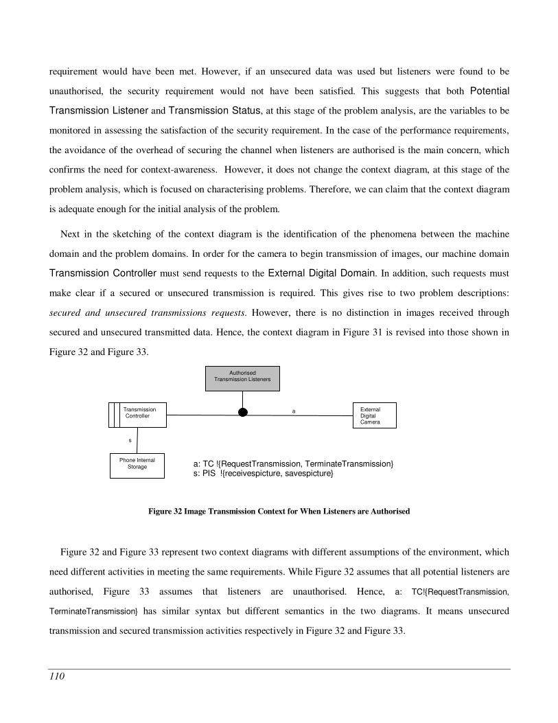
110
requirement would have been met. However, if an unsecured data was used but listeners were found to be
unauthorised, the security requirement would not have been satisfied. This suggests that both Potential
Transmission Listener and Transmission Status, at this stage of the problem analysis, are the variables to be
monitored in assessing the satisfaction of the security requirement. In the case of the performance requirements,
the avoidance of the overhead of securing the channel when listeners are authorised is the main concern, which
confirms the need for context-awareness. However, it does not change the context diagram, at this stage of the
problem analysis, which is focused on characterising problems. Therefore, we can claim that the context diagram
is adequate enough for the initial analysis of the problem.
Next in the sketching of the context diagram is the identification of the phenomena between the machine
domain and the problem domains. In order for the camera to begin transmission of images, our machine domain
Transmission Controller must send requests to the External Digital Domain. In addition, such requests must
make clear if a secured or unsecured transmission is required. This gives rise to two problem descriptions:
secured and unsecured transmissions requests. However, there is no distinction in images received through
secured and unsecured transmitted data. Hence, the context diagram in Figure 31 is revised into those shown in
Figure 32 and Figure 33.
Figure 32 Image Transmission Context for When Listeners are Authorised
Figure 32 and Figure 33 represent two context diagrams with different assumptions of the environment, which
need different activities in meeting the same requirements. While Figure 32 assumes that all potential listeners are
authorised, Figure 33 assumes that listeners are unauthorised. Hence, a: TC!{RequestTransmission,
TerminateTransmission} has similar syntax but different semantics in the two diagrams. It means unsecured
transmission and secured transmission activities respectively in Figure 32 and Figure 33.
Phone Internal Storage
External Digital Camera
Transmission Controller
Authorised Transmission Listeners
a
a: TC !{RequestTransmission, TerminateTransmission} s: PIS !{receivespicture, savespicture}
s
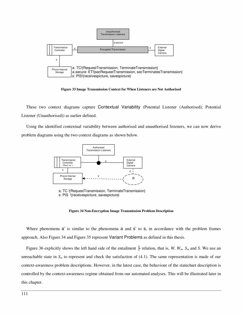
111
Figure 33 Image Transmission Context for When Listeners are Not Authorised
These two context diagrams capture Contextual Variability (Potential Listener (Authorised); Potential
Listener (Unauthorised)) as earlier defined.
Using the identified contextual variability between authorised and unauthorised listeners, we can now derive
problem diagrams using the two context diagrams as shown below.
Figure 34 Non-Encryption Image Transmission Problem Description
Where phenomena a’ is similar to the phenomena a and s’ to s, in accordance with the problem frames
approach. Also Figure 34 and Figure 35 represent Variant Problems as defined in this thesis.
Figure 36 explicitly shows the left hand side of the entailment relation, that is, W, Wm, Sm and S. We use an
unreachable state in Sm to represent and check the satisfaction of (4.1). The same representation is made of our
context-awareness problem descriptions. However, in the latest case, the behaviour of the statechart description is
controlled by the context-awareness regime obtained from our automated analyses. This will be illustrated later in
this chapter.
Phone Internal Storage
External Digital Camera
Transmission Controller
Unauthorised Transmission Listeners
Encrypted Transmission a
a: TC!{RequestTransmission, TerminateTransmission} a-secure: ET!{secRequestTransmission, secTerminatesTransmission} s: PIS!{receivespicture, savespicture}
a-secure
s
a
Phone Internal Storage
External Digital Camera
R
Transmission Controller (SecLoc )
Authorised Transmission Listeners
a: TC !{RequestTransmission, TerminateTransmission} s: PIS !{receivespicture, savespicture}
a
a’ s
s’
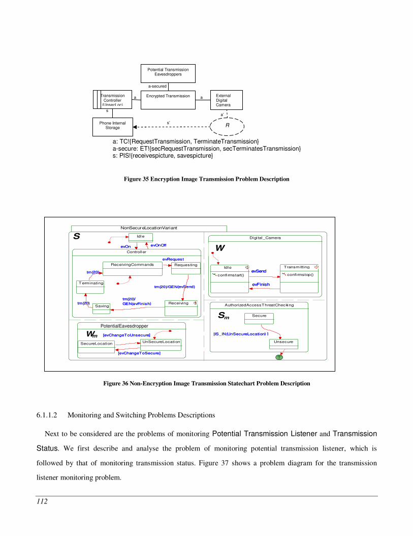
112
Figure 35 Encryption Image Transmission Problem Description
Figure 36 Non-Encryption Image Transmission Statechart Problem Description
6.1.1.2 Monitoring and Switching Problems Descriptions
Next to be considered are the problems of monitoring Potential Transmission Listener and Transmission
Status. We first describe and analyse the problem of monitoring potential transmission listener, which is
followed by that of monitoring transmission status. Figure 37 shows a problem diagram for the transmission
listener monitoring problem.
Phone Internal Storage
External Digital Camera
R
Transmission Controller
(UnsecLoc)
Potential Transmission Eavesdroppers
a
a’ s
s’
Encrypted Transmission
a
a-secured
a: TC!{RequestTransmission, TerminateTransmission} a-secure: ET!{secRequestTransmission, secTerminatesTransmission} s: PIS!{receivespicture, savespicture}
NonSecureLocationVariant
Digi tal_Camera
W
Idle
confi rmstart()
Transmitting
confi rmstop()
evFinish
evSend
AuthorizedAccessThreatChecking
Secure
Unsecure
[IS_IN(UnSecureLocation) ]
Sm
PotentialEarDropper
WUnSecureLocation
m
SecureLocation
[evChangeToUnsecure]
[evChangeToSecure]
Idle
Controller
Saving
Requesting
Terminating
tm(20) Receiving
tm(20)/GEN(evSend)
tm(20)/
GEN(evFinish)
ReceivingCommands
evRequest
tm(20)
evOn evOnOff
evFinish
evSend
[IS_IN(UnSecureLocation) ][evChangeToUnsecure]
[evChangeToSecure]
evOn
tm(20)
tm(20)/GEN(evSend)
tm(20)/
GEN(evFinish)
evRequest
tm(20)
evOnOff
S
PotentialEavesdropper
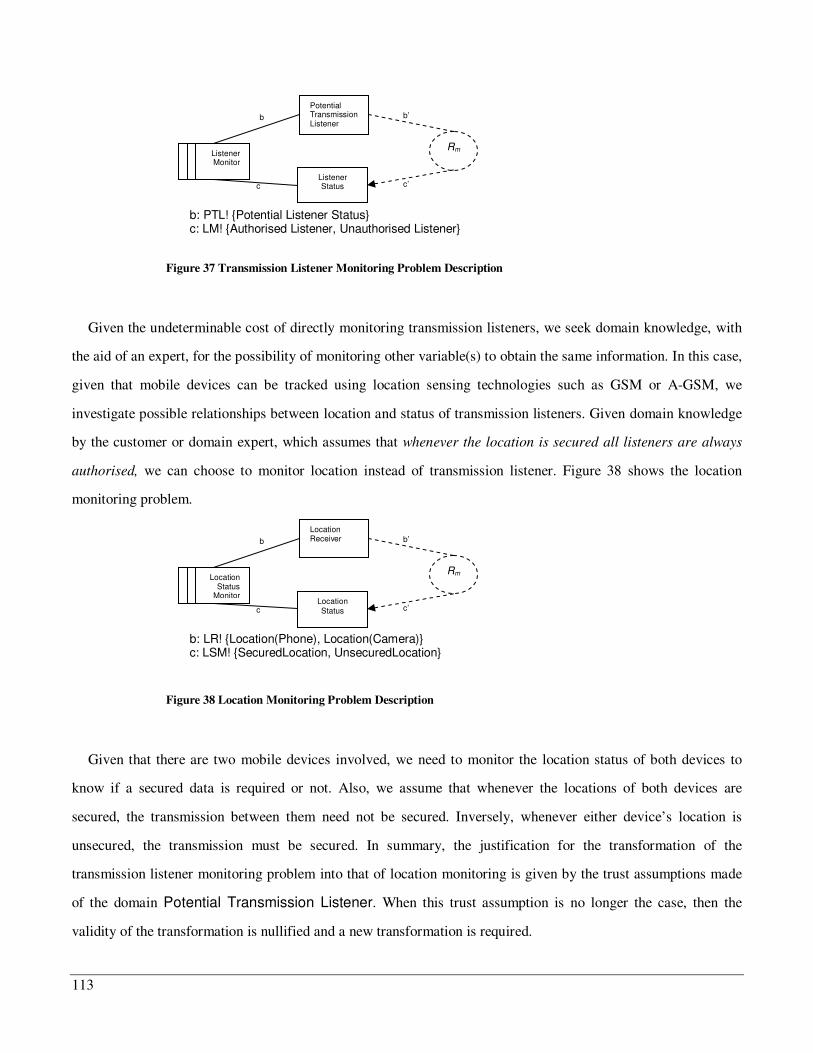
113
Figure 37 Transmission Listener Monitoring Problem Description
Given the undeterminable cost of directly monitoring transmission listeners, we seek domain knowledge, with
the aid of an expert, for the possibility of monitoring other variable(s) to obtain the same information. In this case,
given that mobile devices can be tracked using location sensing technologies such as GSM or A-GSM, we
investigate possible relationships between location and status of transmission listeners. Given domain knowledge
by the customer or domain expert, which assumes that whenever the location is secured all listeners are always
authorised, we can choose to monitor location instead of transmission listener. Figure 38 shows the location
monitoring problem.
Figure 38 Location Monitoring Problem Description
Given that there are two mobile devices involved, we need to monitor the location status of both devices to
know if a secured data is required or not. Also, we assume that whenever the locations of both devices are
secured, the transmission between them need not be secured. Inversely, whenever either device’s location is
unsecured, the transmission must be secured. In summary, the justification for the transformation of the
transmission listener monitoring problem into that of location monitoring is given by the trust assumptions made
of the domain Potential Transmission Listener. When this trust assumption is no longer the case, then the
validity of the transformation is nullified and a new transformation is required.
Rm
b’
c
Listener Monitor
Potential Transmission Listener
Listener Status
b
c’
b: PTL! {Potential Listener Status} c: LM! {Authorised Listener, Unauthorised Listener}
Rm
b’
c
Location Status
Monitor
Location Receiver
Location Status
b
c’
b: LR! {Location(Phone), Location(Camera)} c: LSM! {SecuredLocation, UnsecuredLocation}
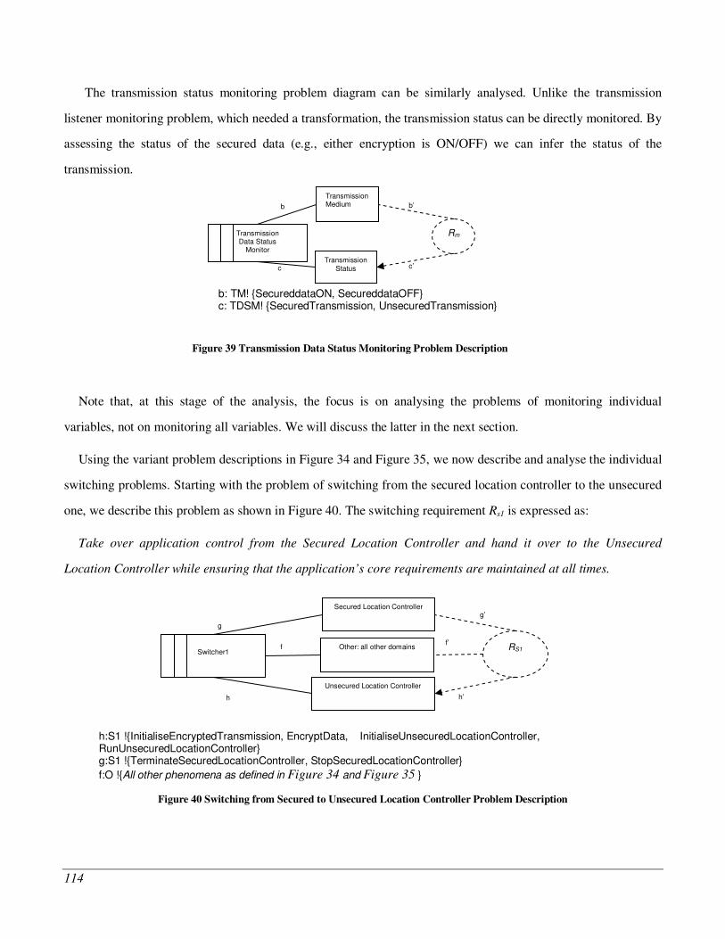
114
The transmission status monitoring problem diagram can be similarly analysed. Unlike the transmission
listener monitoring problem, which needed a transformation, the transmission status can be directly monitored. By
assessing the status of the secured data (e.g., either encryption is ON/OFF) we can infer the status of the
transmission.
Figure 39 Transmission Data Status Monitoring Problem Description
Note that, at this stage of the analysis, the focus is on analysing the problems of monitoring individual
variables, not on monitoring all variables. We will discuss the latter in the next section.
Using the variant problem descriptions in Figure 34 and Figure 35, we now describe and analyse the individual
switching problems. Starting with the problem of switching from the secured location controller to the unsecured
one, we describe this problem as shown in Figure 40. The switching requirement Rs1 is expressed as:
Take over application control from the Secured Location Controller and hand it over to the Unsecured
Location Controller while ensuring that the application’s core requirements are maintained at all times.
Figure 40 Switching from Secured to Unsecured Location Controller Problem Description
Rm
b’
c
Transmission Data Status
Monitor
Transmission Medium
Transmission Status
b
c’
b: TM! {SecureddataON, SecureddataOFF} c: TDSM! {SecuredTransmission, UnsecuredTransmission}
g
h
g’
RS1
Switcher1
Secured Location Controller
Unsecured Location Controller
h’
Other: all other domains f’
f
h:S1 !{InitialiseEncryptedTransmission, EncryptData, InitialiseUnsecuredLocationController, RunUnsecuredLocationController} g:S1 !{TerminateSecuredLocationController, StopSecuredLocationController}
f:O !{All other phenomena as defined in Figure 34 and Figure 35 }

115
From the switching requirement Rs1 above, we deduce that Rs1 R, where R is the mobile application’s core
requirements. Since the Secured Location Controller only transmits data and does no encryption of the transmitted
data, we assume that control can be taken away from it at anytime. This gives rise to the phenomena g:S1
!{TerminateSecuredLocationController, StopSecuredLocationController}. On the other hand, the Unsecured
Location Controller must first encrypt the data before transmission, which gives rise to the phenomena h:S1
!{InitialiseEncryptedTransmission, EncryptData, InitialiseUnsecuredLocationController,
RunUnsecuredLocationController}.
Figure 41 Switching from Unsecured to Secured Location Controller Problem Description
We now consider the switching problem of taking control from the Unsecured Location Controller and handing
it over to the Secured Location Controller. The problem description for this is shown in Figure 41. The switching
requirement Rs2 is expressed as:
Take over application control from the Unsecured Location Controller and hand it over to the Secured Location
Controller while ensuring that the application’s core requirements are maintained at all times.
Again, Rs2 R, where R is the mobile application’s core requirements. Even though the satisfaction of each of
the switching requirements must ensure that of the core requirements, Rs1 R and Rs2 R, the two switching
requirements are not always equivalent Rs1 Rs2 as each presents different problem description. For instance, it is
relatively easier to take control from the Secured Location Controller in comparison to that from the
Unsecured Location Controller. In the latter case, the conditions for switching is not dictated by Rs2 alone as the
g
h
g’
RS2 Switcher2
Secured Location Controller
Unsecured Location Controller
e
Encrypted Transmission
Other: all other domains
e’
h’
f’ f
h:S2 !{CheckEncryptionTransmissionStatus, TerminateEncryptionTransmission, TerminateUnsecuredLocationController, StopUnsecuredLocationController} g:S2 !{InitialiseSecuredLocationController, RunSecuredLocationController} f:ET!{EncryptionStart, EncryptionStop}
e:O !{All other phenomena as defined in Figure 34and Figure 35}
116
state of the data securing activity also has an impact on the switching decision. This explains the differences in
phenomena g:S1 !{TerminateSecuredLocationController, StopSecuredLocationController} and h:S2
!{CheckDataSecuringStatus, TerminateDataSecuring, TerminateUnsecuredLocationController,
StopUnsecuredLocationController}.
In order to check the status of data securing activity, the data securing domain (i.e., its associated variable)
must be added to the list of variables to be monitored as discussed in Section 4.2. In this case, we have added a
variable Encryption Transmission Status to the list which assumes one of three possible states: Initialising, In-
Progress, Terminating. Monitoring this newly added variable, we are able to determine contextual conditions
under which switching is possible in addition to the trade-off setting. In this case, we may switch from the
Unsecured Location Controller to the Secured Location Controller, if location changes from unsecured to
secured, providing the Encrypted Transmission is still being initialised. While the encryption status is being
monitored, we can monitor the size of the image data being transmitted to determine if data securing should be
aborted and the file retransmitted without encryption. Alternatively, transmission may be allowed to continue,
however, given the extra information obtained from the image size monitoring, we are not able to categorise the
performance requirement satisfaction level. As an example, if securing is unnecessarily performed with a small
image file, then the performance satisfaction level is partially satisfied. It would be partially denied if the image
file was large and unnecessary data securing took place.
From the analysis for problem classification and for both monitoring and switching, we have so far elicited the
following variables: Transmission Listener Status; Location Status; Encryption Transmission Status; and
Image Size Status.
6.1.1.3 Analyse Monitoring and Switching Conditions
Using the elicited variables in the previous section, we illustrate how Contextual dependency is captured as
constraints in propositions, how they are used to analyse monitoring and switching conditions and to simulate
context-aware (behaviour) specifications.
Altogether, we encoded 31 propositions into 479 cnf rules as input to SAT4J. We now present the encoding of
(4.4) into propositional formula in our automated analysis tool, illustrating how some of the 31 propositions are
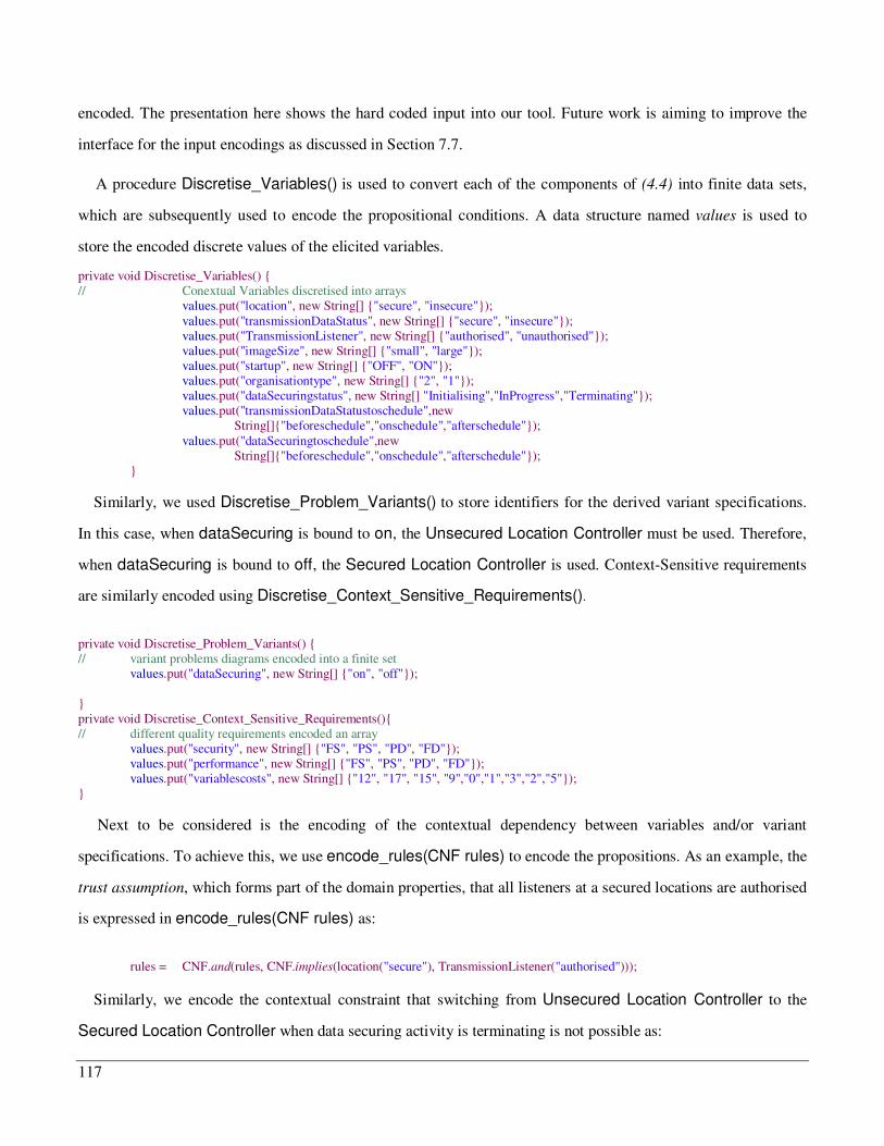
117
encoded. The presentation here shows the hard coded input into our tool. Future work is aiming to improve the
interface for the input encodings as discussed in Section 7.7.
A procedure Discretise_Variables() is used to convert each of the components of (4.4) into finite data sets,
which are subsequently used to encode the propositional conditions. A data structure named values is used to
store the encoded discrete values of the elicited variables.
private void Discretise_Variables() { // Conextual Variables discretised into arrays values.put("location", new String[] {"secure", "insecure"}); values.put("transmissionDataStatus", new String[] {"secure", "insecure"}); values.put("TransmissionListener", new String[] {"authorised", "unauthorised"}); values.put("imageSize", new String[] {"small", "large"}); values.put("startup", new String[] {"OFF", "ON"}); values.put("organisationtype", new String[] {"2", "1"}); values.put("dataSecuringstatus", new String[] "Initialising","InProgress","Terminating"}); values.put("transmissionDataStatustoschedule",new
String[]{"beforeschedule","onschedule","afterschedule"}); values.put("dataSecuringtoschedule",new
String[]{"beforeschedule","onschedule","afterschedule"}); }
Similarly, we used Discretise_Problem_Variants() to store identifiers for the derived variant specifications.
In this case, when dataSecuring is bound to on, the Unsecured Location Controller must be used. Therefore,
when dataSecuring is bound to off, the Secured Location Controller is used. Context-Sensitive requirements
are similarly encoded using Discretise_Context_Sensitive_Requirements().
private void Discretise_Problem_Variants() { // variant problems diagrams encoded into a finite set values.put("dataSecuring", new String[] {"on", "off"}); } private void Discretise_Context_Sensitive_Requirements(){ // different quality requirements encoded an array values.put("security", new String[] {"FS", "PS", "PD", "FD"}); values.put("performance", new String[] {"FS", "PS", "PD", "FD"}); values.put("variablescosts", new String[] {"12", "17", "15", "9","0","1","3","2","5"}); }
Next to be considered is the encoding of the contextual dependency between variables and/or variant
specifications. To achieve this, we use encode_rules(CNF rules) to encode the propositions. As an example, the
trust assumption, which forms part of the domain properties, that all listeners at a secured locations are authorised
is expressed in encode_rules(CNF rules) as:
rules = CNF.and(rules, CNF.implies(location("secure"), TransmissionListener("authorised")));
Similarly, we encode the contextual constraint that switching from Unsecured Location Controller to the
Secured Location Controller when data securing activity is terminating is not possible as:
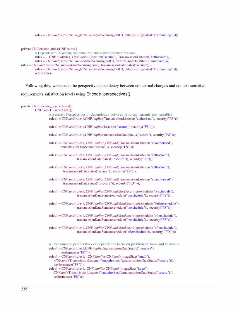
118
rules = CNF.and(rules,CNF.neg(CNF.and(dataSecuring("off"), dataSecuringstatus("Terminating"))));
private CNF encode_rules(CNF rules) { // Dependenc rules among contextual variables and/or problem variants rules = CNF.and(rules, CNF.implies(location("secure"), TransmissionListener("authorised"))); rules = CNF.and(rules,CNF.implies(dataSecuring("off"), transmissionDataStatus("insecure"))); rules = CNF.and(rules,CNF.implies(dataSecuring("on"), transmissionDataStatus("secure"))); rules = CNF.and(rules,CNF.neg(CNF.and(dataSecuring("off"), dataSecuringstatus("Terminating")))); return rules; }
Following this, we encode the perspective dependency between contextual changes and context-sensitive
requirements satisfaction levels using Encode_perspectives().
private CNF Encode_perspectives(){ CNF rules1 = new CNF(); // Security Perspectives of dependency between problem variants and variables rules1 = CNF.and(rules1,CNF.implies(TransmissionListener("authorised"), security("FS"))); rules1 = CNF.and(rules1,CNF.implies(location("secure"), security("FS"))); rules1 = CNF.and(rules1,CNF.implies(transmissionDataStatus("secure"), security("FS"))); rules1 = CNF.and(rules1, CNF.implies(CNF.and(TransmissionListener("unauthorised"),
transmissionDataStatus("secure")), security("FS")));
rules1 = CNF.and(rules1, CNF.implies(CNF.and(TransmissionListener("authorised"), transmissionDataStatus("insecure")), security("FS")));
rules1 = CNF.and(rules1, CNF.implies(CNF.and(TransmissionListener("authorised"), transmissionDataStatus("secure")), security("FS")));
rules1 = CNF.and(rules1, CNF.implies(CNF.and(TransmissionListener("unauthorised"), transmissionDataStatus("insecure")), security("FD")));
rules1 = CNF.and(rules1, CNF.implies(CNF.and(dataSecuringtoschedule("onschedule"), transmissionDataStatustoschedule("onschedule")), security("FS")));
rules1 = CNF.and(rules1, CNF.implies(CNF.and(dataSecuringtoschedule("beforeschedule"), transmissionDataStatustoschedule("onschedule")), security("FS")));
rules1 = CNF.and(rules1, CNF.implies(CNF.and(dataSecuringtoschedule("afterschedule"), transmissionDataStatustoschedule("onschedule")), security("FS")));
rules1 = CNF.and(rules1, CNF.implies(CNF.and(dataSecuringtoschedule("afterschedule"), transmissionDataStatustoschedule("afterschedule")), security("FD")));
// Performance perspectives of dependency between problem variants and variables rules1 = CNF.and(rules1,CNF.implies(transmissionDataStatus("insecure"), performance("FS"))); rules1 = CNF.and(rules1, CNF.implies(CNF.and (imageSize("small"), CNF.and (TransmissionListener("unauthorised"),transmissionDataStatus("secure"))), performance("PS"))); rules1 = CNF.and(rules1, CNF.implies(CNF.and (imageSize("large"), CNF.and (TransmissionListener("unauthorised"),transmissionDataStatus("secure"))), performance("PD")));
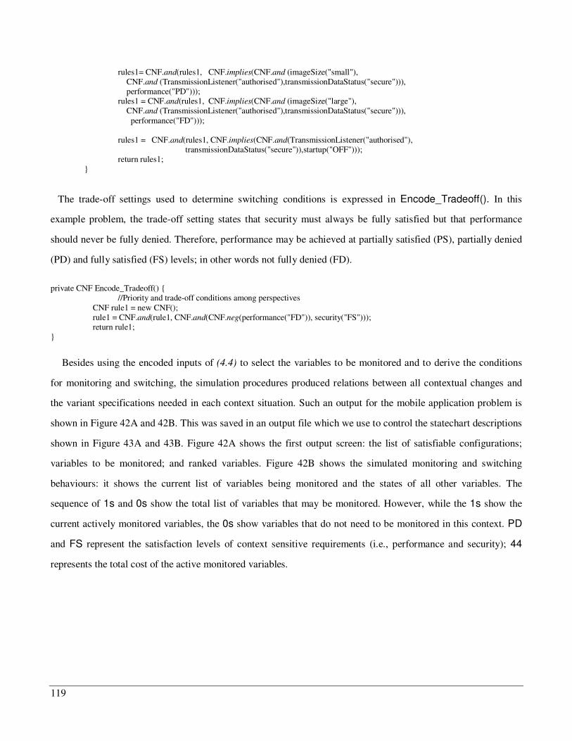
119
rules1= CNF.and(rules1, CNF.implies(CNF.and (imageSize("small"), CNF.and (TransmissionListener("authorised"),transmissionDataStatus("secure"))), performance("PD"))); rules1 = CNF.and(rules1, CNF.implies(CNF.and (imageSize("large"), CNF.and (TransmissionListener("authorised"),transmissionDataStatus("secure"))), performance("FD"))); rules1 = CNF.and(rules1, CNF.implies(CNF.and(TransmissionListener("authorised"), transmissionDataStatus("secure")),startup("OFF"))); return rules1; }
The trade-off settings used to determine switching conditions is expressed in Encode_Tradeoff(). In this
example problem, the trade-off setting states that security must always be fully satisfied but that performance
should never be fully denied. Therefore, performance may be achieved at partially satisfied (PS), partially denied
(PD) and fully satisfied (FS) levels; in other words not fully denied (FD).
private CNF Encode_Tradeoff() { //Priority and trade-off conditions among perspectives CNF rule1 = new CNF(); rule1 = CNF.and(rule1, CNF.and(CNF.neg(performance("FD")), security("FS"))); return rule1; }
Besides using the encoded inputs of (4.4) to select the variables to be monitored and to derive the conditions
for monitoring and switching, the simulation procedures produced relations between all contextual changes and
the variant specifications needed in each context situation. Such an output for the mobile application problem is
shown in Figure 42A and 42B. This was saved in an output file which we use to control the statechart descriptions
shown in Figure 43A and 43B. Figure 42A shows the first output screen: the list of satisfiable configurations;
variables to be monitored; and ranked variables. Figure 42B shows the simulated monitoring and switching
behaviours: it shows the current list of variables being monitored and the states of all other variables. The
sequence of 1s and 0s show the total list of variables that may be monitored. However, while the 1s show the
current actively monitored variables, the 0s show variables that do not need to be monitored in this context. PD
and FS represent the satisfaction levels of context sensitive requirements (i.e., performance and security); 44
represents the total cost of the active monitored variables.
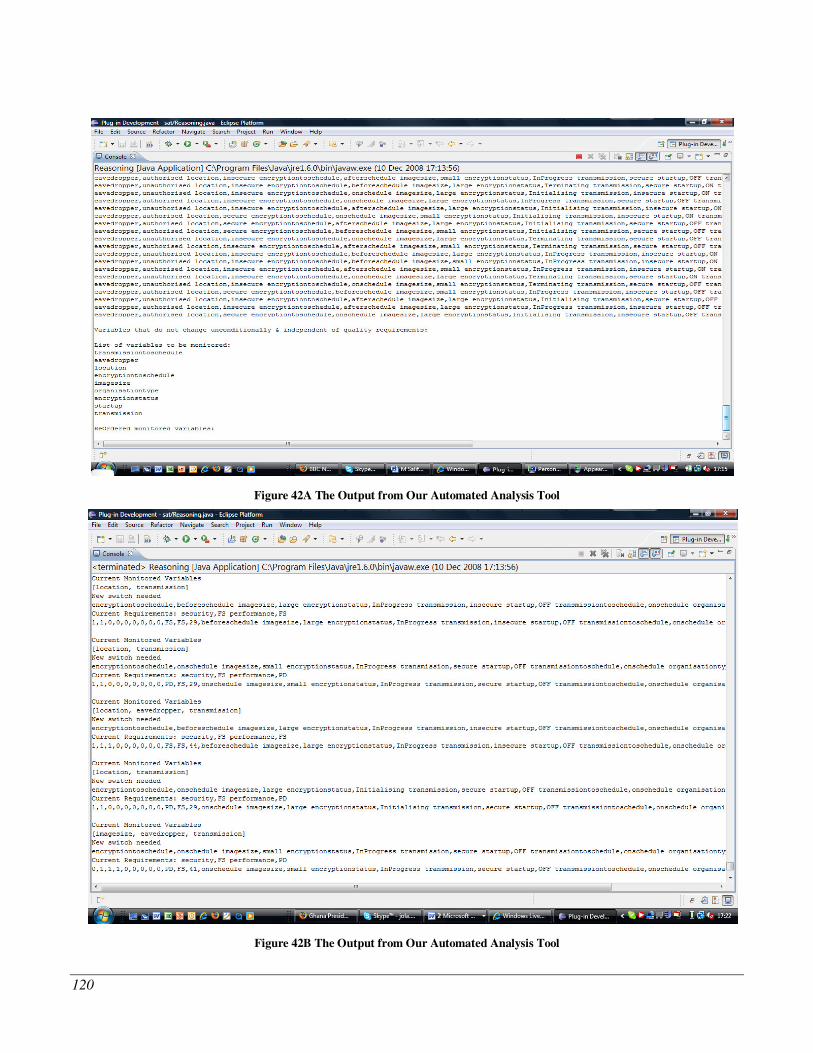
120
Figure 42A The Output from Our Automated Analysis Tool
Figure 42B The Output from Our Automated Analysis Tool
121
As a summary, in this section, we have shown how contextual variables are partitioned; contextual
dependency between variables and variant specifications encoded into propositions; perspective contextual
dependency between contextual variables and context-sensitive requirements encoded into SAT rules; and trade-
offs values between context-sensitive requirements encoded into SAT rules. Also, we have shown how the inputs
are encoded as discrete values internal to the SAT-Solver (SAT4J). Propositions are given either positive or
negative numbers and used as input to the SAT4J Solver. In addition, we have shown how the encoded inputs are
used by our automated tool to derive monitoring and switching conditions which are used to simulate context-
awareness behaviour specification.
In the next section, we discuss how the output from the tool is used as the underlying control ‘engine’ for the
context-aware problem description in statechart models.
6.1.2 Statechart -based Description of Context-Awareness
The statechart description for the context-aware problem and its simulations are shown in Figure 43A and
43B, which take into account the output from the tool. In Figure 43A and 43B, domains such as sub-problem
specifications S, S;S, Sm and their contexts; and the specification for the context switcher Ss, are treated as state
machines. Note that the Encrypting state could have been described in detailed state description in terms of its
sub-states Initialising, In-progress and Terminating. Such information is useful to analyse initialisation and
termination concerns during variant switching. Using this level of detail, we are able to specify that switching is
possible from UnsecLocVariant to SecLocVariant during transmission, providing that encryption has not
entered the Terminating state.
Using the IS_IN(x) function, we now briefly discuss how temporal information in statechart is encoded into
SAT proposition. Although not visible in Figure 43A and 43B but considered in the constraint problem analysis,
Encrypting can be exited if it is in either the Initialising or In-progress states but not when it is in the
Terminating state. Such temporal constraints can be expressed as SAT input as:
dep(EncryptionInitialising ^ EavesdropperAuthorised, SwitcherUnSecuredMode) = (EncryptionInitialising ^ EavesdropperAuthorised) implies
SwitcherUnSecuredMode dep(EncryptionInProgress^EavesdropperAuthorised, SwitcherUnSecuredMode) = (EncryptionInProgres ^ EavesdropperAuthorised) implies
SwitcherUnSecuredMode
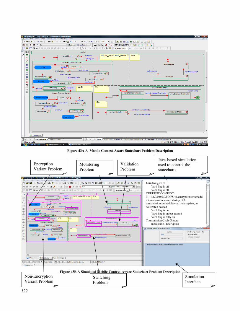
122
Figure 43A A Mobile Context-Aware Statechart Problem Description
Figure 43B A Simulated Mobile Context-Aware Statechart Problem Description
Monitoring Problem
Validation Problem
Java-based simulation used to control the statecharts
Switching Problem
Encryption Variant Problem
Initialising GUI … Var1 flag is off Var0 flag is off CURRENT CONTEXT: 0,1,1,1,0,0,0,0,0,PD,FS,41,encryption,onschedule transmission,secure startup,OFF transmissiontoscheduletype,1 encryption,on No switch needed Var1 flag is on Var1 flag is on but paused Var1 flag is fully on Transmission Cycle Started Initialising, Encrypting
Simulation Interface
Non-Encryption Variant Problem
123
Similarly: dep(EncryptionTerminating ^EavesdropperAuthorised, SwitcherSecuredMode) = (EncryptionTerminating ^ EavesdropperAuthorised) implies
SwitcherSecuredMode
dep(Encryption ^EavesdropperUnAuthorised, SwitcherSecuredMode) = (Encryption ^ EavesdropperUnAuthorised) implies SwitcherSecuredMode
Each of these is transformed into a CNF equivalent. As an example:
dep(EncryptionInitilising^EavesdropperAuthorised, SwitcherUnSecuredMode) is transformed into CNF equivalent as:
!(EncryptionInitilising ^ EavesdropperAuthorised) ) SwitcherUnSecuredMode
This is how we encode information extracted from statechart description as part of our constraint problem in (4).
Figure 43A shows a statechart problem description of the mobile application. This is the view in Telelogic
Rhapsody before simulation. All states and state machines are shown in green. Figure 43B shows the simulated
statechart. The highlighted states and state machines in purple show active states. The upper right screen shows
the current context change that is simulated in a Java API which links the statechart description to the output from
our tool (shown in Figure 42B). The caption CURRENT CONTEXT lists the current variables partition and the
required variant specification needed in such a partition, which corresponds to the output from our tool. The lower
right screen shows a GUI interface which one can use to control contextual changes while one can observe its
effect on the statechart model, which must reflect changes in the upper right screen.
Besides simulating the required context-awareness behaviour using the statechart description, we are able to
capture a sequence of executions which are saved into a standard text file. Using the saved data, we can compare
monitoring and switching behaviour to assess the impact of using contextual dependency to refine context-
awareness behaviour. We next discuss the results of such comparisons.
6.1.3 Impact of Our Monitoring and Switching Theorems on Context-Awareness
6.1.3.1 Impact of Monitoring Theory on Monitoring Behaviour
In the mobile application problem, we elicited a total of six variables, each taking one of two possible values.
These are Location, Listener-status, Transmission-status, Image-size, Startup and Organisation-type.
Organisation-type was added to test that the tool accurately identifies it as a variable that must never be
124
monitored. The startup variable was used to express variable combinations that are not permissible at application
start time, which offers us some temporal capability. Our tool detects that it is not necessary to monitor the
organisation-type and startup variables. Organisation-type has no impact on requirements. Although the startup
variable has impact on requirements, the tool identified that its status can already be established while monitoring
transmission-type. Of the remaining four variables, transmission-type is unconditionally monitored; location,
listener-status and image-size are conditionally monitored using the derived dependencies. Each variable is
assigned a monitoring cost by domain experts. Even though we recognised that the cost of monitoring is not a
direct function of the number of variables monitored, we nevertheless find it useful in analysing the impact of
using our monitoring theory to control monitoring behaviour. Using the assigned cost, we are able to compare the
cost of monitoring which is controlled by our monitoring theorem (Monitoring2) and those that are not controlled
by it (Monitoring1). Figure 44 compares the varying number and cost of monitored variables induced by
Monitoring2 and the constant number and cost of monitored variables induced by Monitoring1. More importantly,
the Monitoring2 and Cost2 show the number of variables monitored and the cost of monitoring reduced.
Considering the variable curves, Monitoring2 and Cost2, Figure 44 shows, in intervals 0 to 10 and 50 to 60,
situations where you have a fixed number of variables being monitored but not a fixed (i.e. the same) set of
variables. Hence, an apparent constant in the number of monitored variables with non-constant cost of monitoring
aligned in the same time intervals. This phenomenon is caused by the differences in the cost of monitoring each
contextual variable. When monitoring different variables provides the same information, the tool monitors the
variable of the least cost.
6.1.3.2 Impact of Switching Theory on Switching Behaviour
The output from the tool also enables us to compare switching which is controlled by our switching theorem
(Switching2) and those not controlled by it (Switching1). Using our theory, switching must always be essential.
Essential change occurs when and only when the current context changes and variant problem do not satisfy the
given trade-off values. Over the number of analysed contextual changes, the frequency of switching in Switching2
is lower than that of Switching1. This is reflected by 18 switches in the Switching2 curve and 24 in the
Switching1 curve, out of over 60 changes.
Figure 45 also compares the impact on context-sensitive requirements of carrying out our theory controlled
switching. Given that the security requirement is fully satisfied in all contexts, Figure 45 compares only

125
performance requirement satisfaction levels (i.e., performance satisfaction1 and satisfaction2). Performance1
curve produced FS=23, PS=22 and PD=18 against that of the performance2 switching induced curve producing
FS=23, PS = 14 and PD = 26. As can be seen, the efficiency is analysed in terms of switching behaviour not in the
satisfaction level of performance. The underlying constraint is that the trade-of value must never be satisfied.
6.1.3.3 Impact of Trade-off Changes on Context-Sensitive Requirements Satisfaction
Given the dependency of our two theories on the trade-off of context-sensitive requirements, changes to the
values of the trade-off will induce different monitoring and switching behaviours. The security requirement in our
mobile application problem has been set to Fully Satisfied in the analysis so far. As an example, we revised the
trade-off values such that the security requirement may be Fully Denied and the performance requirement must
never by fully denied, which results in the modified satisfaction levels both security and performance as shown in
Figure 46.
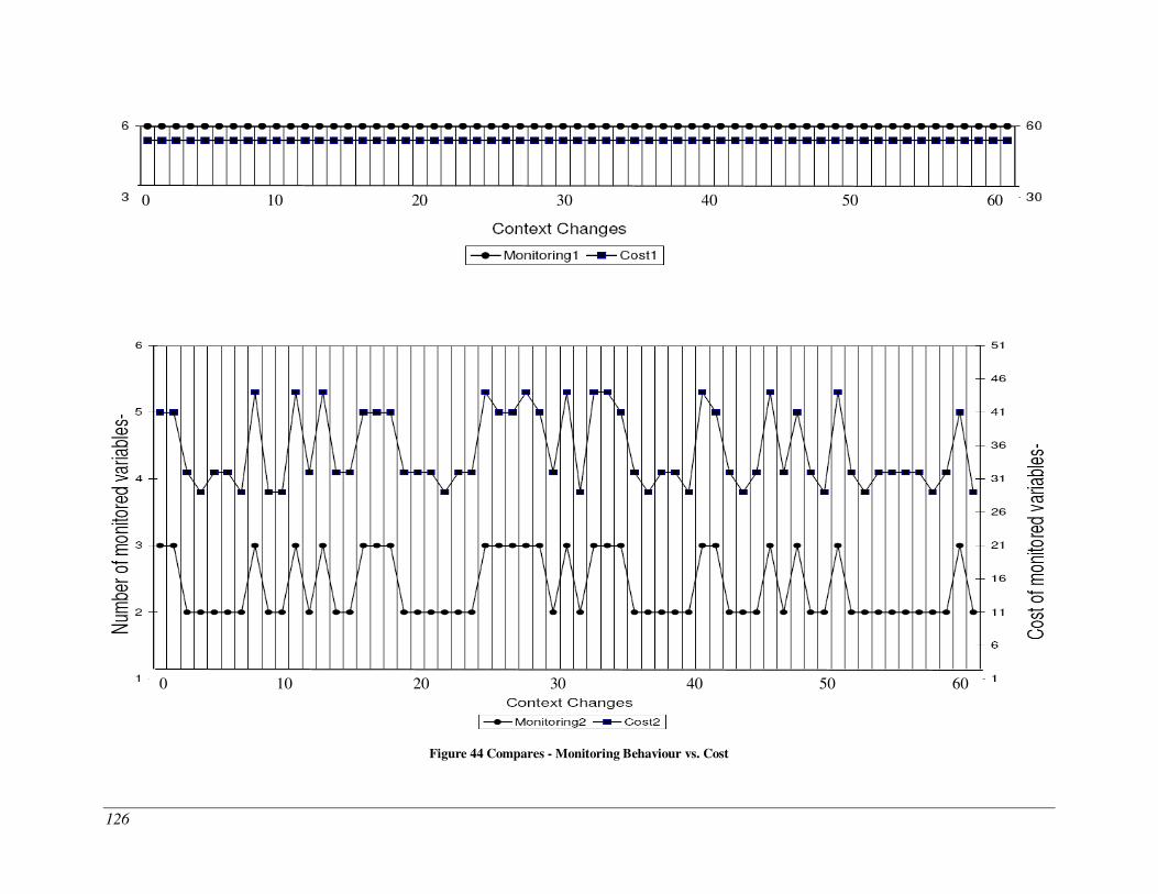
126
Figure 44 Compares - Monitoring Behaviour vs. Cost
0 10 20 30 40 50 60
0 10 20 30 40 50 60
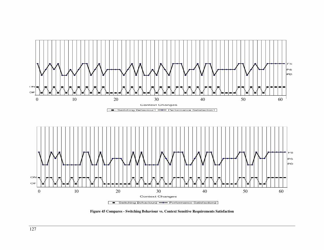
127
Figure 45 Compares - Switching Behaviour vs. Context Sensitive Requirements Satisfaction
0 10 20 30 40 50 60
0 10 20 30 40 50 60
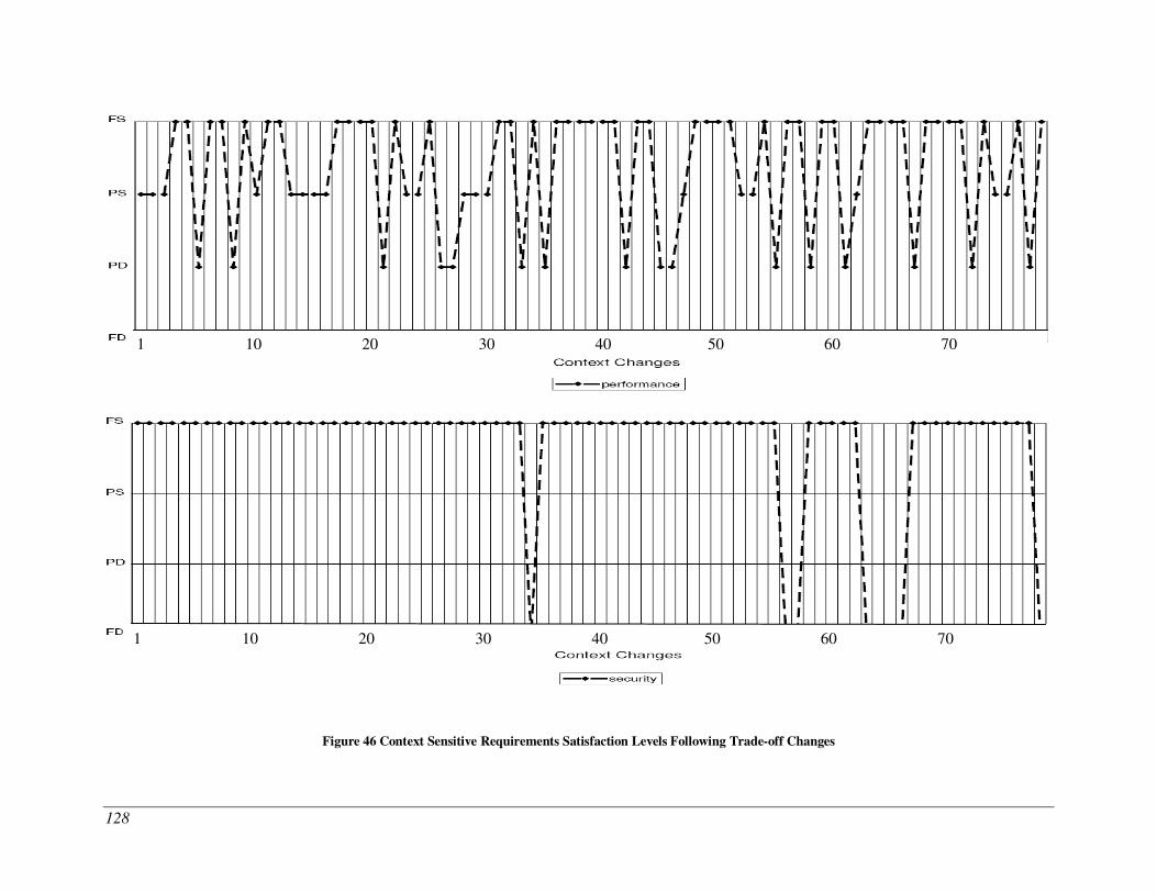
128
Figure 46 Context Sensitive Requirements Satisfaction Levels Following Trade-off Changes
1 10 20 30 40 50 60 70
1 10 20 30 40 50 60 70
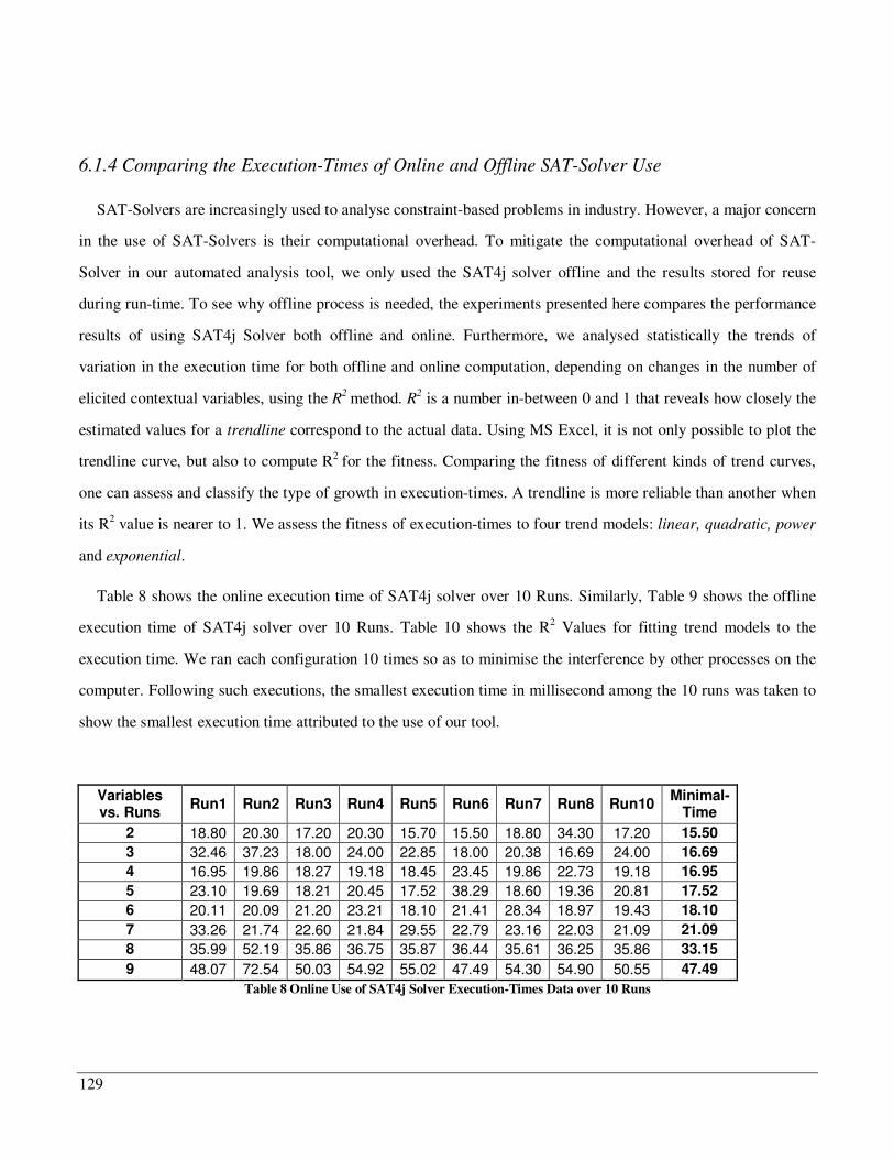
129
6.1.4 Comparing the Execution-Times of Online and Offline SAT-Solver Use
SAT-Solvers are increasingly used to analyse constraint-based problems in industry. However, a major concern
in the use of SAT-Solvers is their computational overhead. To mitigate the computational overhead of SAT-
Solver in our automated analysis tool, we only used the SAT4j solver offline and the results stored for reuse
during run-time. To see why offline process is needed, the experiments presented here compares the performance
results of using SAT4j Solver both offline and online. Furthermore, we analysed statistically the trends of
variation in the execution time for both offline and online computation, depending on changes in the number of
elicited contextual variables, using the R2 method. R2 is a number in-between 0 and 1 that reveals how closely the
estimated values for a trendline correspond to the actual data. Using MS Excel, it is not only possible to plot the
trendline curve, but also to compute R2 for the fitness. Comparing the fitness of different kinds of trend curves,
one can assess and classify the type of growth in execution-times. A trendline is more reliable than another when
its R2 value is nearer to 1. We assess the fitness of execution-times to four trend models: linear, quadratic, power
and exponential.
Table 8 shows the online execution time of SAT4j solver over 10 Runs. Similarly, Table 9 shows the offline
execution time of SAT4j solver over 10 Runs. Table 10 shows the R2 Values for fitting trend models to the
execution time. We ran each configuration 10 times so as to minimise the interference by other processes on the
computer. Following such executions, the smallest execution time in millisecond among the 10 runs was taken to
show the smallest execution time attributed to the use of our tool.
Variables vs. Runs
Run1 Run2 Run3 Run4 Run5 Run6 Run7 Run8 Run10 Minimal-
Time
2 18.80 20.30 17.20 20.30 15.70 15.50 18.80 34.30 17.20 15.50
3 32.46 37.23 18.00 24.00 22.85 18.00 20.38 16.69 24.00 16.69
4 16.95 19.86 18.27 19.18 18.45 23.45 19.86 22.73 19.18 16.95
5 23.10 19.69 18.21 20.45 17.52 38.29 18.60 19.36 20.81 17.52
6 20.11 20.09 21.20 23.21 18.10 21.41 28.34 18.97 19.43 18.10
7 33.26 21.74 22.60 21.84 29.55 22.79 23.16 22.03 21.09 21.09
8 35.99 52.19 35.86 36.75 35.87 36.44 35.61 36.25 35.86 33.15
9 48.07 72.54 50.03 54.92 55.02 47.49 54.30 54.90 50.55 47.49
Table 8 Online Use of SAT4j Solver Execution-Times Data over 10 Runs
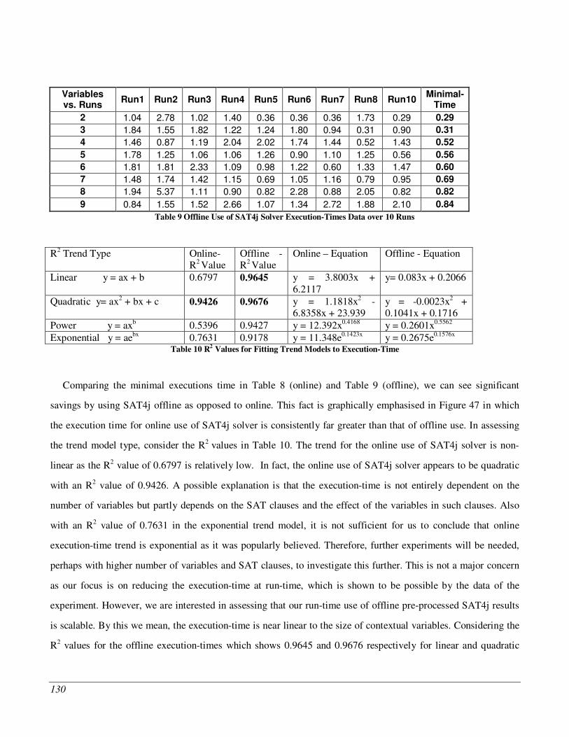
130
Variables vs. Runs
Run1 Run2 Run3 Run4 Run5 Run6 Run7 Run8 Run10 Minimal-
Time
2 1.04 2.78 1.02 1.40 0.36 0.36 0.36 1.73 0.29 0.29
3 1.84 1.55 1.82 1.22 1.24 1.80 0.94 0.31 0.90 0.31
4 1.46 0.87 1.19 2.04 2.02 1.74 1.44 0.52 1.43 0.52
5 1.78 1.25 1.06 1.06 1.26 0.90 1.10 1.25 0.56 0.56
6 1.81 1.81 2.33 1.09 0.98 1.22 0.60 1.33 1.47 0.60
7 1.48 1.74 1.42 1.15 0.69 1.05 1.16 0.79 0.95 0.69
8 1.94 5.37 1.11 0.90 0.82 2.28 0.88 2.05 0.82 0.82
9 0.84 1.55 1.52 2.66 1.07 1.34 2.72 1.88 2.10 0.84
Table 9 Offline Use of SAT4j Solver Execution-Times Data over 10 Runs
R2 Trend Type Online-R2 Value
Offline - R2 Value
Online – Equation Offline - Equation
Linear y = ax + b 0.6797 0.9645 y = 3.8003x + 6.2117
y= 0.083x + 0.2066
Quadratic y= ax2 + bx + c 0.9426 0.9676 y = 1.1818x2 - 6.8358x + 23.939
y = -0.0023x2 + 0.1041x + 0.1716
Power y = axb 0.5396 0.9427 y = 12.392x0.4168 y = 0.2601x0.5562 Exponential y = aebx 0.7631 0.9178 y = 11.348e0.1423x y = 0.2675e0.1576x
Table 10 R2 Values for Fitting Trend Models to Execution-Time
Comparing the minimal executions time in Table 8 (online) and Table 9 (offline), we can see significant
savings by using SAT4j offline as opposed to online. This fact is graphically emphasised in Figure 47 in which
the execution time for online use of SAT4j solver is consistently far greater than that of offline use. In assessing
the trend model type, consider the R2 values in Table 10. The trend for the online use of SAT4j solver is non-
linear as the R2 value of 0.6797 is relatively low. In fact, the online use of SAT4j solver appears to be quadratic
with an R2 value of 0.9426. A possible explanation is that the execution-time is not entirely dependent on the
number of variables but partly depends on the SAT clauses and the effect of the variables in such clauses. Also
with an R2 value of 0.7631 in the exponential trend model, it is not sufficient for us to conclude that online
execution-time trend is exponential as it was popularly believed. Therefore, further experiments will be needed,
perhaps with higher number of variables and SAT clauses, to investigate this further. This is not a major concern
as our focus is on reducing the execution-time at run-time, which is shown to be possible by the data of the
experiment. However, we are interested in assessing that our run-time use of offline pre-processed SAT4j results
is scalable. By this we mean, the execution-time is near linear to the size of contextual variables. Considering the
R2 values for the offline execution-times which shows 0.9645 and 0.9676 respectively for linear and quadratic
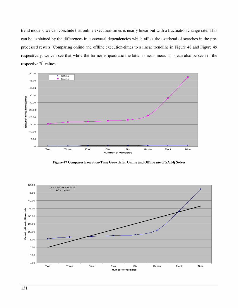
131
trend models, we can conclude that online execution-times is nearly linear but with a fluctuation change rate. This
can be explained by the differences in contextual dependencies which affect the overhead of searches in the pre-
processed results. Comparing online and offline execution-times to a linear trendline in Figure 48 and Figure 49
respectively, we can see that while the former is quadratic the latter is near-linear. This can also be seen in the
respective R2 values.
0.00
5.00
10.00
15.00
20.00
25.00
30.00
35.00
40.00
45.00
50.00
Two Three Four Five Six Seven Eight Nine
Number of Variables
Execution-T
imes in M
ilis
econds
Offline
Online
Figure 47 Compares Execution-Time Growth for Online and Offline use of SAT4j Solver
y = 3.8003x + 6.2117
R2 = 0.6797
0.00
5.00
10.00
15.00
20.00
25.00
30.00
35.00
40.00
45.00
50.00
Two Three Four Five Six Seven Eight Nine
Number of Variables
Execution-T
imes in M
ilis
econds
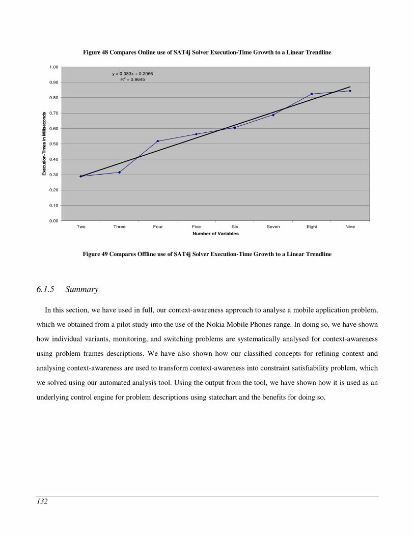
132
Figure 48 Compares Online use of SAT4j Solver Execution-Time Growth to a Linear Trendline
y = 0.083x + 0.2066
R2 = 0.9645
0.00
0.10
0.20
0.30
0.40
0.50
0.60
0.70
0.80
0.90
1.00
Two Three Four Five Six Seven Eight Nine
Number of Variables
Execution-T
imes in M
ilis
econds
Figure 49 Compares Offline use of SAT4j Solver Execution-Time Growth to a Linear Trendline
6.1.5 Summary
In this section, we have used in full, our context-awareness approach to analyse a mobile application problem,
which we obtained from a pilot study into the use of the Nokia Mobile Phones range. In doing so, we have shown
how individual variants, monitoring, and switching problems are systematically analysed for context-awareness
using problem frames descriptions. We have also shown how our classified concepts for refining context and
analysing context-awareness are used to transform context-awareness into constraint satisfiability problem, which
we solved using our automated analysis tool. Using the output from the tool, we have shown how it is used as an
underlying control engine for problem descriptions using statechart and the benefits for doing so.
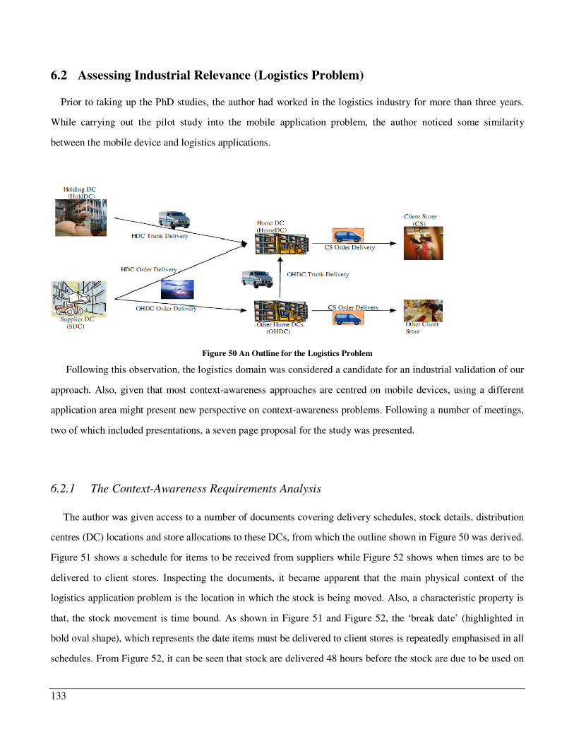
133
6.2 Assessing Industrial Relevance (Logistics Problem)
Prior to taking up the PhD studies, the author had worked in the logistics industry for more than three years.
While carrying out the pilot study into the mobile application problem, the author noticed some similarity
between the mobile device and logistics applications.
Figure 50 An Outline for the Logistics Problem
Following this observation, the logistics domain was considered a candidate for an industrial validation of our
approach. Also, given that most context-awareness approaches are centred on mobile devices, using a different
application area might present new perspective on context-awareness problems. Following a number of meetings,
two of which included presentations, a seven page proposal for the study was presented.
6.2.1 The Context-Awareness Requirements Analysis
The author was given access to a number of documents covering delivery schedules, stock details, distribution
centres (DC) locations and store allocations to these DCs, from which the outline shown in Figure 50 was derived.
Figure 51 shows a schedule for items to be received from suppliers while Figure 52 shows when times are to be
delivered to client stores. Inspecting the documents, it became apparent that the main physical context of the
logistics application problem is the location in which the stock is being moved. Also, a characteristic property is
that, the stock movement is time bound. As shown in Figure 51 and Figure 52, the ‘break date’ (highlighted in
bold oval shape), which represents the date items must be delivered to client stores is repeatedly emphasised in all
schedules. From Figure 52, it can be seen that stock are delivered 48 hours before the stock are due to be used on
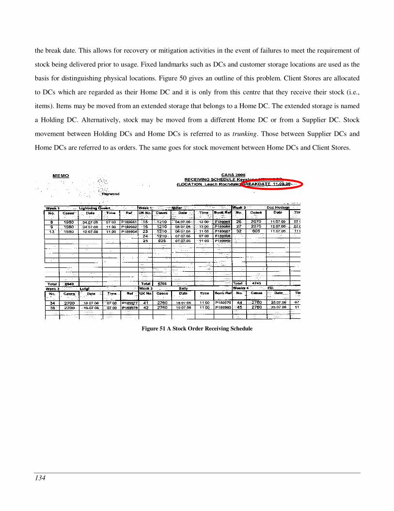
134
the break date. This allows for recovery or mitigation activities in the event of failures to meet the requirement of
stock being delivered prior to usage. Fixed landmarks such as DCs and customer storage locations are used as the
basis for distinguishing physical locations. Figure 50 gives an outline of this problem. Client Stores are allocated
to DCs which are regarded as their Home DC and it is only from this centre that they receive their stock (i.e.,
items). Items may be moved from an extended storage that belongs to a Home DC. The extended storage is named
a Holding DC. Alternatively, stock may be moved from a different Home DC or from a Supplier DC. Stock
movement between Holding DCs and Home DCs is referred to as trunking. Those between Supplier DCs and
Home DCs are referred to as orders. The same goes for stock movement between Home DCs and Client Stores.
Figure 51 A Stock Order Receiving Schedule
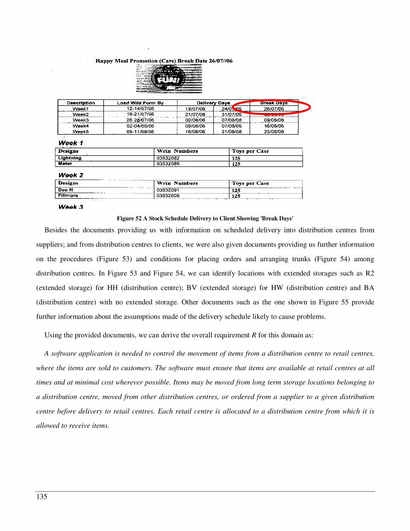
135
Figure 52 A Stock Schedule Delivery to Client Showing 'Break Days'
Besides the documents providing us with information on scheduled delivery into distribution centres from
suppliers; and from distribution centres to clients, we were also given documents providing us further information
on the procedures (Figure 53) and conditions for placing orders and arranging trunks (Figure 54) among
distribution centres. In Figure 53 and Figure 54, we can identify locations with extended storages such as R2
(extended storage) for HH (distribution centre); BV (extended storage) for HW (distribution centre) and BA
(distribution centre) with no extended storage. Other documents such as the one shown in Figure 55 provide
further information about the assumptions made of the delivery schedule likely to cause problems.
Using the provided documents, we can derive the overall requirement R for this domain as:
A software application is needed to control the movement of items from a distribution centre to retail centres,
where the items are sold to customers. The software must ensure that items are available at retail centres at all
times and at minimal cost wherever possible. Items may be moved from long term storage locations belonging to
a distribution centre, moved from other distribution centres, or ordered from a supplier to a given distribution
centre before delivery to retail centres. Each retail centre is allocated to a distribution centre from which it is
allowed to receive items.

136
Figure 53 Item Order into Storage Location Procedure
Figure 54 Guidelines for Item Trunking between Storage Locations

137
Figure 55 Possible Assumptions about Item Movement Likely to Cause Problems
6.2.1.1 Analyse Problems for Different Contexts
In analysing the derived requirements, we start with the assumption that there is always sufficient stock in the
Home DC to be delivered to the customer; Figure 56 shows the variant problem descriptions suitable for this
context.
Figure 56 Variant for when Stock is Available Problem Description
R
C5
CM1!C1
Control Machine1
Customer Store
Distribution DC
CS!C2
C3
DDC!C4
CM1!C1{PrepareStockForCustomer, SendStockToCustomer,StopStockToCustomer, ScheduledArrivalTime} CS!C2{ReceiveStockFromDC}, CS!C3 {ReceiveOrderFromDC} DDC!C3 {PrepareOrderForCustomer, SendOrderToCustomer,StopOrderToCustomer, ScheduledArrivalTime} DDC!C4!{TransportStocktoCustomer, ActualArrivalTime} CS!C5!{CustomerReceivesDelivery, CustomerConfirmsReceiptOfDelivery}
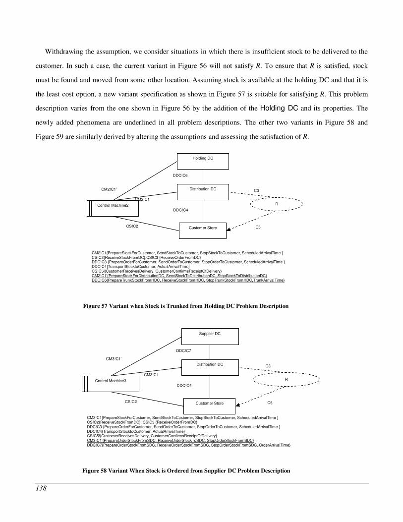
138
Withdrawing the assumption, we consider situations in which there is insufficient stock to be delivered to the
customer. In such a case, the current variant in Figure 56 will not satisfy R. To ensure that R is satisfied, stock
must be found and moved from some other location. Assuming stock is available at the holding DC and that it is
the least cost option, a new variant specification as shown in Figure 57 is suitable for satisfying R. This problem
description varies from the one shown in Figure 56 by the addition of the Holding DC and its properties. The
newly added phenomena are underlined in all problem descriptions. The other two variants in Figure 58 and
Figure 59 are similarly derived by altering the assumptions and assessing the satisfaction of R.
Figure 57 Variant when Stock is Trunked from Holding DC Problem Description
Figure 58 Variant When Stock is Ordered from Supplier DC Problem Description
R
C5
CM3!C1
Control Machine3
Distribution DC
CS!C2
C3
DDC!C4
Supplier DC
DDC!C7
CM3!C1{PrepareStockForCustomer, SendStockToCustomer, StopStockToCustomer, ScheduledArrivalTime } CS!C2{ReceiveStockFromDC}, CS!C3 {ReceiveOrderFromDC} DDC!C3 {PrepareOrderForCustomer, SendOrderToCustomer, StopOrderToCustomer, ScheduledArrivalTime } DDC!C4{TransportStocktoCustomer, ActualArrivalTime} CS!C5!{CustomerReceivesDelivery, CustomerConfirmsReceiptOfDelivery} CM3!C1’{PrepareOrderStockFromSDC, ReceiveOrderStockToSDC, StopOrderStockFromSDC} DDC!C7{PrepareOrderStockFromSDC, ReceiveOrderStockFromSDC, StopOrderStockFromSDC, OrderArrivalTime}
CM3!C1’
Customer Store
R
C5
CM2!C1
Control Machine2
Customer Store
Distribution DC
CS!C2
C3
DDC!C4
Holding DC
DDC!C6
CM2!C1{PrepareStockForCustomer, SendStockToCustomer, StopStockToCustomer, ScheduledArrivalTime } CS!C2{ReceiveStockFromDC},CS!C3 {ReceiveOrderFromDC} DDC!C3 {PrepareOrderForCustomer, SendOrderToCustomer, StopOrderToCustomer, ScheduledArrivalTime } DDC!C4{TransportStocktoCustomer, ActualArrivalTime} CS!C5!{CustomerReceivesDelivery, CustomerConfirmsReceiptOfDelivery} CM2!C1’{PrepareStockForDistributionDC, SendStockToDistributionDC, StopStockToDistributionDC} DDC!C6{PrepareTrunkStockFromHDC, ReceiveStockFromHDC, StopTrunkStockFromHDC,TrunkArrivalTime}
CM2!C1’
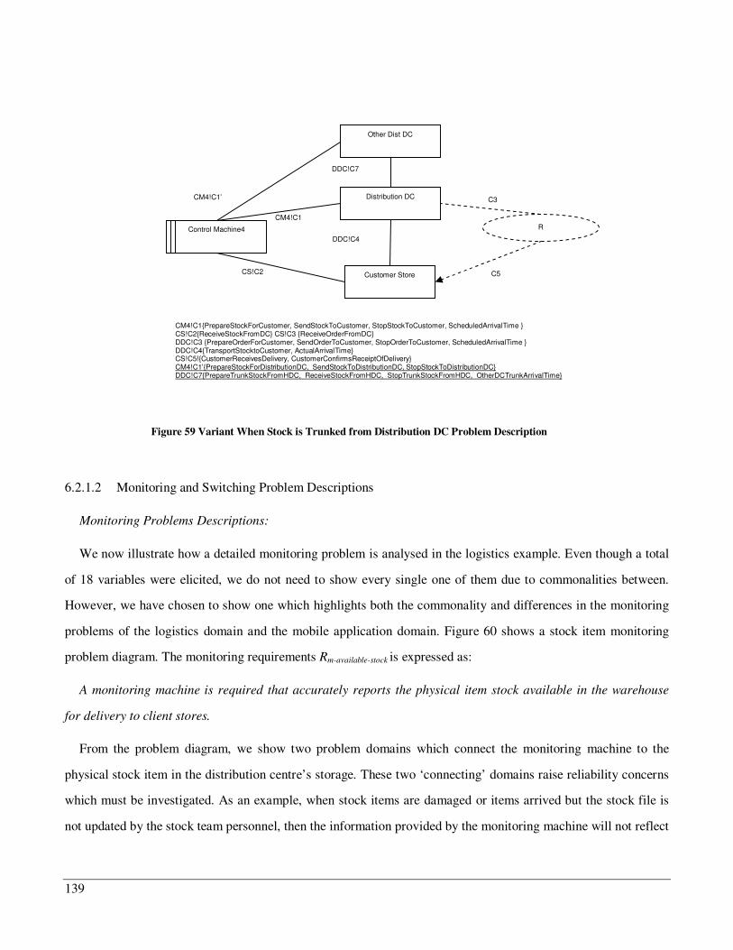
139
Figure 59 Variant When Stock is Trunked from Distribution DC Problem Description
6.2.1.2 Monitoring and Switching Problem Descriptions
Monitoring Problems Descriptions:
We now illustrate how a detailed monitoring problem is analysed in the logistics example. Even though a total
of 18 variables were elicited, we do not need to show every single one of them due to commonalities between.
However, we have chosen to show one which highlights both the commonality and differences in the monitoring
problems of the logistics domain and the mobile application domain. Figure 60 shows a stock item monitoring
problem diagram. The monitoring requirements Rm-available-stock is expressed as:
A monitoring machine is required that accurately reports the physical item stock available in the warehouse
for delivery to client stores.
From the problem diagram, we show two problem domains which connect the monitoring machine to the
physical stock item in the distribution centre’s storage. These two ‘connecting’ domains raise reliability concerns
which must be investigated. As an example, when stock items are damaged or items arrived but the stock file is
not updated by the stock team personnel, then the information provided by the monitoring machine will not reflect
R
C5
CM4!C1
Control Machine4
Customer Store
Distribution DC
CS!C2
C3
DDC!C4
Other Dist DC
DDC!C7
CM4!C1{PrepareStockForCustomer, SendStockToCustomer, StopStockToCustomer, ScheduledArrivalTime } CS!C2{ReceiveStockFromDC} CS!C3 {ReceiveOrderFromDC} DDC!C3 {PrepareOrderForCustomer, SendOrderToCustomer, StopOrderToCustomer, ScheduledArrivalTime } DDC!C4{TransportStocktoCustomer, ActualArrivalTime} CS!C5!{CustomerReceivesDelivery, CustomerConfirmsReceiptOfDelivery} CM4!C1’{PrepareStockForDistributionDC, SendStockToDistributionDC, StopStockToDistributionDC} DDC!C7{PrepareTrunkStockFromHDC, ReceiveStockFromHDC, StopTrunkStockFromHDC, OtherDCTrunkArrivalTime}
CM4!C1’
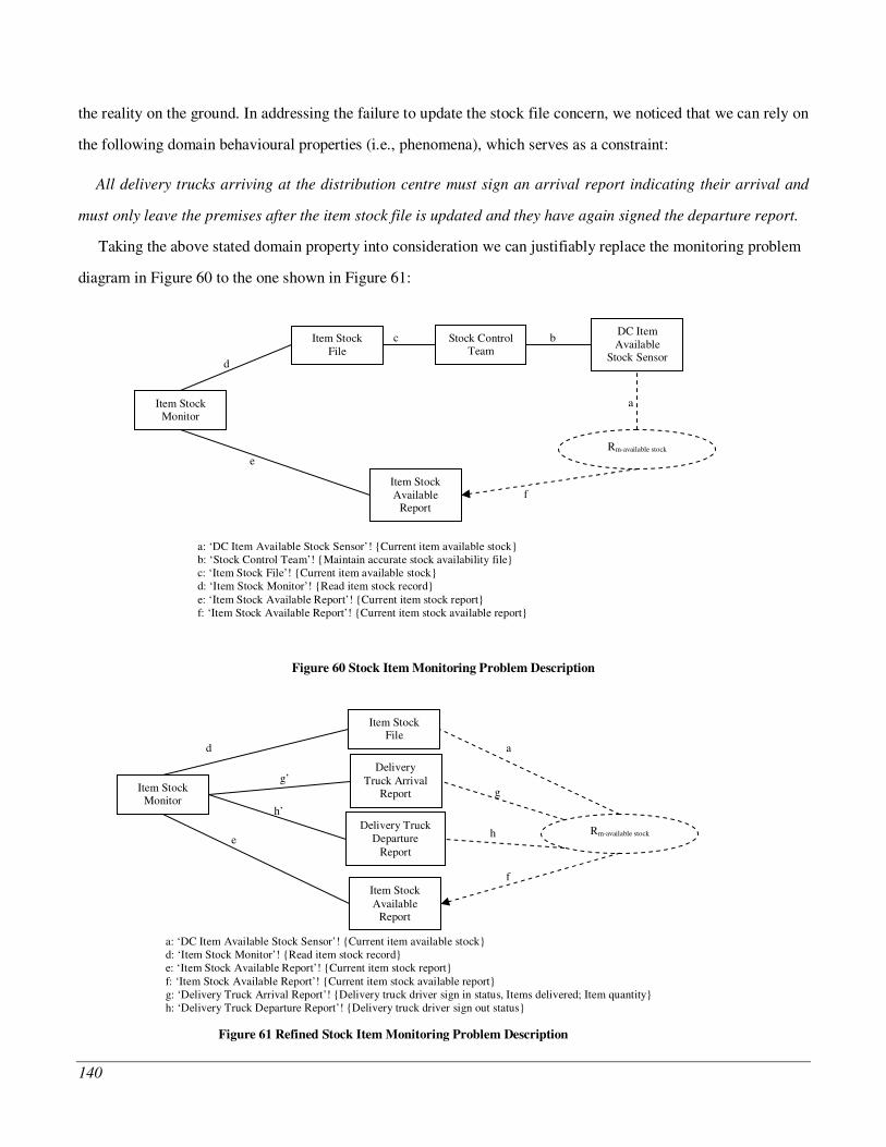
140
the reality on the ground. In addressing the failure to update the stock file concern, we noticed that we can rely on
the following domain behavioural properties (i.e., phenomena), which serves as a constraint:
All delivery trucks arriving at the distribution centre must sign an arrival report indicating their arrival and
must only leave the premises after the item stock file is updated and they have again signed the departure report.
Taking the above stated domain property into consideration we can justifiably replace the monitoring problem
diagram in Figure 60 to the one shown in Figure 61:
Figure 60 Stock Item Monitoring Problem Description
DC Item Available
Stock Sensor
Stock Control Team
Item Stock Monitor
Item Stock Available
Report
Item Stock File
Rm-available stock
d
a
b
e
c
f
a: ‘DC Item Available Stock Sensor’! {Current item available stock} b: ‘Stock Control Team’! {Maintain accurate stock availability file} c: ‘Item Stock File’! {Current item available stock} d: ‘Item Stock Monitor’! {Read item stock record} e: ‘Item Stock Available Report’! {Current item stock report} f: ‘Item Stock Available Report’! {Current item stock available report}
Item Stock Monitor
Item Stock Available
Report
Item Stock File
Rm-available stock
d a
e
f
a: ‘DC Item Available Stock Sensor’! {Current item available stock} d: ‘Item Stock Monitor’! {Read item stock record} e: ‘Item Stock Available Report’! {Current item stock report} f: ‘Item Stock Available Report’! {Current item stock available report} g: ‘Delivery Truck Arrival Report’! {Delivery truck driver sign in status, Items delivered; Item quantity} h: ‘Delivery Truck Departure Report’! {Delivery truck driver sign out status}
Delivery Truck Arrival
Report
Delivery Truck Departure
Report
g
h
g’
h’
Figure 61 Refined Stock Item Monitoring Problem Description
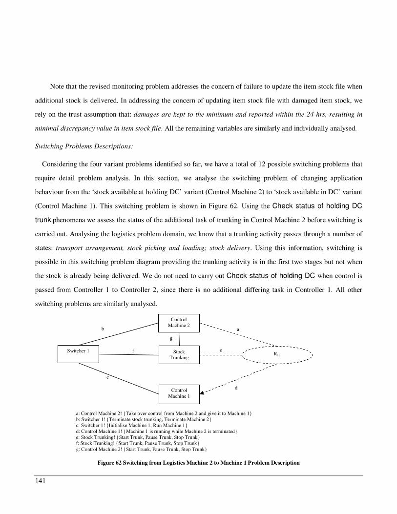
141
Note that the revised monitoring problem addresses the concern of failure to update the item stock file when
additional stock is delivered. In addressing the concern of updating item stock file with damaged item stock, we
rely on the trust assumption that: damages are kept to the minimum and reported within the 24 hrs, resulting in
minimal discrepancy value in item stock file. All the remaining variables are similarly and individually analysed.
Switching Problems Descriptions:
Considering the four variant problems identified so far, we have a total of 12 possible switching problems that
require detail problem analysis. In this section, we analyse the switching problem of changing application
behaviour from the ‘stock available at holding DC’ variant (Control Machine 2) to ‘stock available in DC’ variant
(Control Machine 1). This switching problem is shown in Figure 62. Using the Check status of holding DC
trunk phenomena we assess the status of the additional task of trunking in Control Machine 2 before switching is
carried out. Analysing the logistics problem domain, we know that a trunking activity passes through a number of
states: transport arrangement, stock picking and loading; stock delivery. Using this information, switching is
possible in this switching problem diagram providing the trunking activity is in the first two stages but not when
the stock is already being delivered. We do not need to carry out Check status of holding DC when control is
passed from Controller 1 to Controller 2, since there is no additional differing task in Controller 1. All other
switching problems are similarly analysed.
Figure 62 Switching from Logistics Machine 2 to Machine 1 Problem Description
Switcher 1
Control Machine 1
Control Machine 2
Rs1
b a
c
d
Stock Trunking
e f
g
a: Control Machine 2! {Take over control from Machine 2 and give it to Machine 1} b: Switcher 1! {Terminate stock trunking, Terminate Machine 2} c: Switcher 1! {Initialise Machine 1, Run Machine 1} d: Control Machine 1! {Machine 1 is running while Machine 2 is terminated} e: Stock Trunking! {Start Trunk, Pause Trunk, Stop Trunk} f: Stock Trunking! {Start Trunk, Pause Trunk, Stop Trunk} g: Control Machine 2! {Start Trunk, Pause Trunk, Stop Trunk}
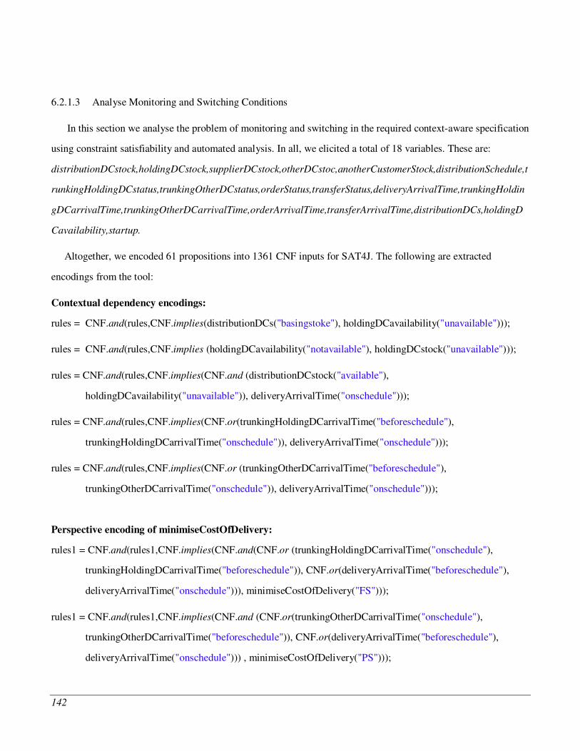
142
6.2.1.3 Analyse Monitoring and Switching Conditions
In this section we analyse the problem of monitoring and switching in the required context-aware specification
using constraint satisfiability and automated analysis. In all, we elicited a total of 18 variables. These are:
distributionDCstock,holdingDCstock,supplierDCstock,otherDCstoc,anotherCustomerStock,distributionSchedule,t
runkingHoldingDCstatus,trunkingOtherDCstatus,orderStatus,transferStatus,deliveryArrivalTime,trunkingHoldin
gDCarrivalTime,trunkingOtherDCarrivalTime,orderArrivalTime,transferArrivalTime,distributionDCs,holdingD
Cavailability,startup.
Altogether, we encoded 61 propositions into 1361 CNF inputs for SAT4J. The following are extracted
encodings from the tool:
Contextual dependency encodings:
rules = CNF.and(rules,CNF.implies(distributionDCs("basingstoke"), holdingDCavailability("unavailable")));
rules = CNF.and(rules,CNF.implies (holdingDCavailability("notavailable"), holdingDCstock("unavailable")));
rules = CNF.and(rules,CNF.implies(CNF.and (distributionDCstock("available"),
holdingDCavailability("unavailable")), deliveryArrivalTime("onschedule")));
rules = CNF.and(rules,CNF.implies(CNF.or(trunkingHoldingDCarrivalTime("beforeschedule"),
trunkingHoldingDCarrivalTime("onschedule")), deliveryArrivalTime("onschedule")));
rules = CNF.and(rules,CNF.implies(CNF.or (trunkingOtherDCarrivalTime("beforeschedule"),
trunkingOtherDCarrivalTime("onschedule")), deliveryArrivalTime("onschedule")));
Perspective encoding of minimiseCostOfDelivery:
rules1 = CNF.and(rules1,CNF.implies(CNF.and(CNF.or (trunkingHoldingDCarrivalTime("onschedule"),
trunkingHoldingDCarrivalTime("beforeschedule")), CNF.or(deliveryArrivalTime("beforeschedule"),
deliveryArrivalTime("onschedule"))), minimiseCostOfDelivery("FS")));
rules1 = CNF.and(rules1,CNF.implies(CNF.and (CNF.or(trunkingOtherDCarrivalTime("onschedule"),
trunkingOtherDCarrivalTime("beforeschedule")), CNF.or(deliveryArrivalTime("beforeschedule"),
deliveryArrivalTime("onschedule"))) , minimiseCostOfDelivery("PS")));
143
Tradeoff encoding :
rule1 = CNF.and(rule1, CNF.neg(stockAvailability("FD")));
This effectively, states that stockAvailability must not be fully denied (FD).
6.2.2 Process-based Description of Context-Awareness
Using the output from our automated analysis tool, we describe the required context-awareness specification
using Figure 63 to Figure 66. While Figure 63 shows a simulated run of the context-awareness specification,
Figure 64 to Figure 66 give the detailed process models for the Home DC stock available variant, the
monitoring, and the switching specifications respectively. Problem domain phenomena are represented as tasks in
process models; and the problem domains for which they belong to attached to them as resources. In Figure 63,
(lower) the curved rectangles without the plus sign represent atomic tasks while those with the sign represent sub-
processes which we detail in Figure 64 to Figure 66. Therefore, Composed Monitoring and Switching represent
the sub-processes for monitoring and switching respectively, while Running Distribution DC Variant represents
a local task within the context-awareness process.
Control dependencies are elicited by considering the input and output connections. As an example, in Figure
66, we elicit that Deriving Target Variant must precede Switching Variants. More general dependency
information is extracted from inputs and outputs constraints which are represented using the logical operators
AND, OR, IS EQUAL TO, IS LESS THAN, IS GREATER THAN. These are WebSphere tool specific. In order
to achieve the effect of the IS_IN(x) function in Rhapsody, which allows one to detect state changes in other state
machines parallel to the state in which it is used, WebSphere uses data repositories. This allows a sub-process to
exchange data with its parent process. A data repository may be atomic, which shows direct connections to inputs
and outputs ports or global, which maintains only virtual connections without explicit links to input and outputs
(as shown in the Composed Monitoring in Figure 63). Given that data is either written to a repository using an
output, or read from one using an input, constraints on inputs and outputs can include data elements in
repositories. Therefore, outputs from the simulated procedures in our tool are imported into global repositories
144
which are used by the monitoring and switching procedure in Figure 63. For an example of how dependency
information in process models are encoded into SAT propositions, consider the following:
(Switching.Switcher.Input Criterion.Input.monitoring_report. allocated_quantity
IS GREATER THAN
Switching.Switcher.Input Criterion.Input.monitoring_report.localDC_stock _quantity)
AND
( Switching.Switcher.Input Criterion.Input.monitoring_report.allocated_quantity
IS LESS THAN
Switching.Switcher.Input Criterion.Input.monitoring _ report.holdingDC-stock_quantity)
From the above expression: Switching is the name of the process model; Switcher the name of the decision
point (task); Input Criterion confirms that it constraints the input; the specific input is Input1; the data element
associated with this input is monitoring_report; and the specific attribute of the element is the
allocated_quantity. All other sub-expressions are similarly related.
These process model constraints can be encoded into SAT as:
dep(DistributionDCStockInSufficient ^ HoldingDCStockSufficient, HoldingDCVariantRunningOn)
= (DistributionDCStockInSufficient ^ HoldingDCStockSufficient) implies HoldingDCVariantRunningON
We have shown only two variants in the process model problem description so as to enhance legibility due to
the static printout out medium. This does not affect the technical argument and presentation of our context-
awareness problem description using process modelling.
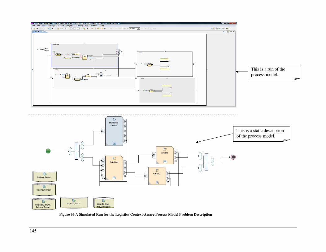
145
Figure 63 A Simulated Run for the Logistics Context-Aware Process Model Problem Description
This is a run of the process model.
This is a static description of the process model.
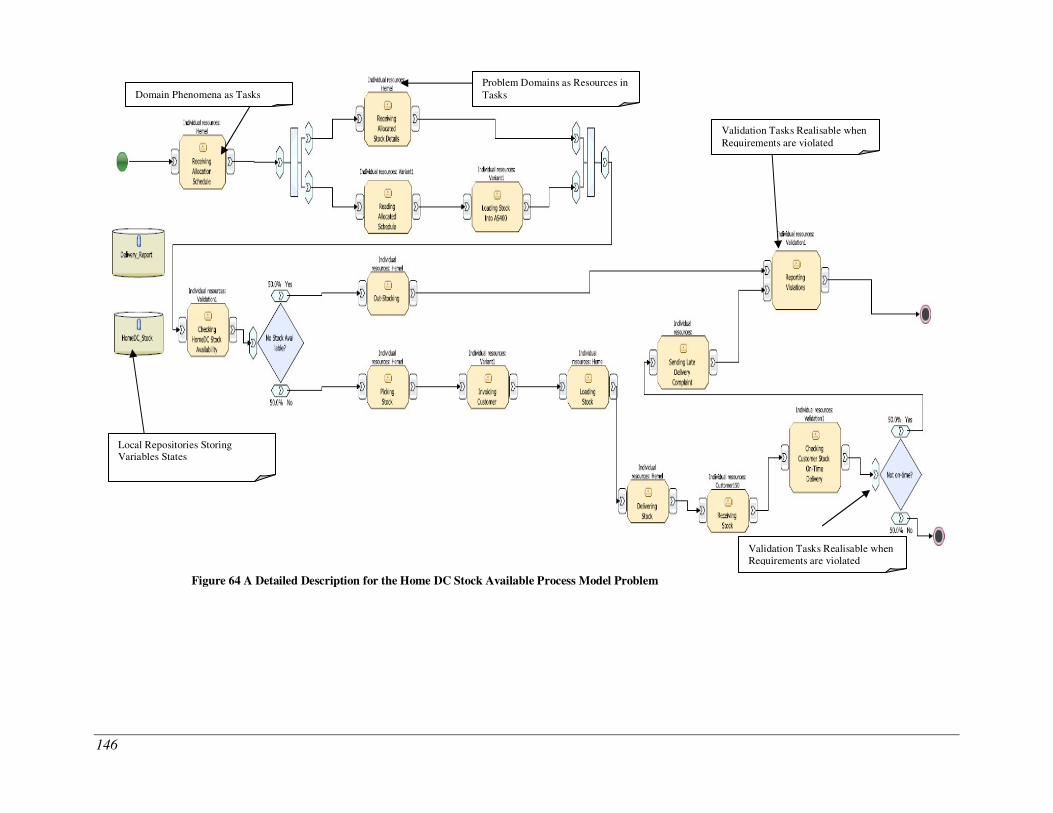
146
Figure 64 A Detailed Description for the Home DC Stock Available Process Model Problem
Validation Tasks Realisable when Requirements are violated
Problem Domains as Resources in Tasks
Validation Tasks Realisable when Requirements are violated
Domain Phenomena as Tasks
Local Repositories Storing Variables States
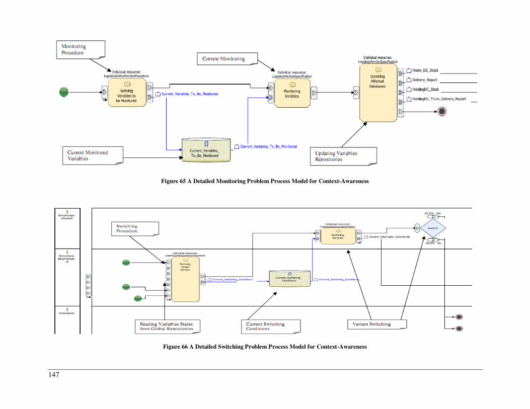
147
Figure 65 A Detailed Monitoring Problem Process Model for Context-Awareness
Figure 66 A Detailed Switching Problem Process Model for Context-Awareness
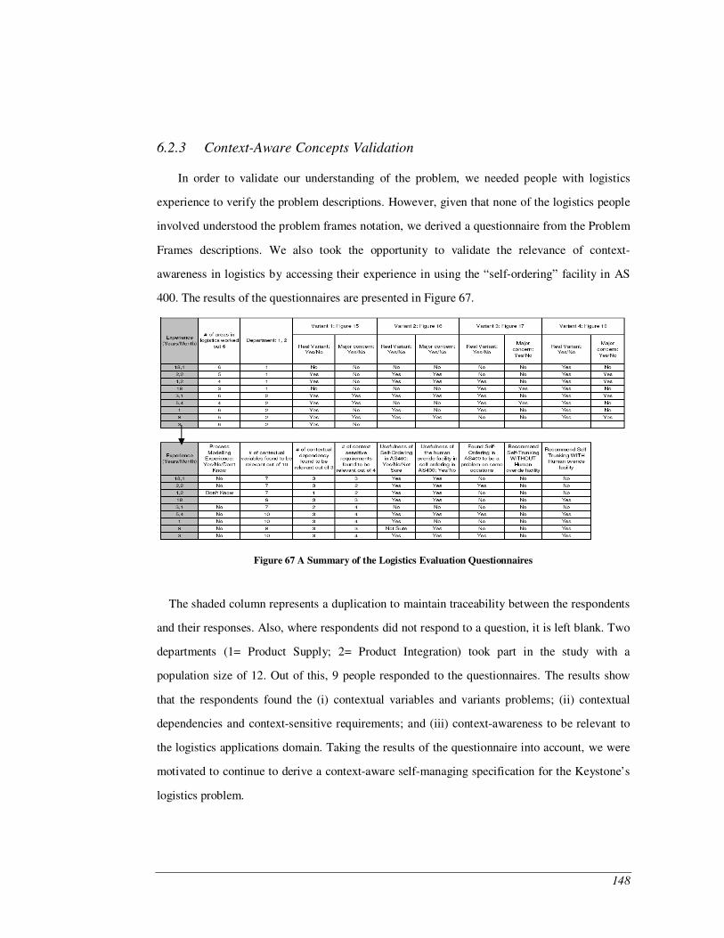
148
6.2.3 Context-Aware Concepts Validation
In order to validate our understanding of the problem, we needed people with logistics
experience to verify the problem descriptions. However, given that none of the logistics people
involved understood the problem frames notation, we derived a questionnaire from the Problem
Frames descriptions. We also took the opportunity to validate the relevance of context-
awareness in logistics by accessing their experience in using the “self-ordering” facility in AS
400. The results of the questionnaires are presented in Figure 67.
Figure 67 A Summary of the Logistics Evaluation Questionnaires
The shaded column represents a duplication to maintain traceability between the respondents
and their responses. Also, where respondents did not respond to a question, it is left blank. Two
departments (1= Product Supply; 2= Product Integration) took part in the study with a
population size of 12. Out of this, 9 people responded to the questionnaires. The results show
that the respondents found the (i) contextual variables and variants problems; (ii) contextual
dependencies and context-sensitive requirements; and (iii) context-awareness to be relevant to
the logistics applications domain. Taking the results of the questionnaire into account, we were
motivated to continue to derive a context-aware self-managing specification for the Keystone’s
logistics problem.
149
The behaviour of this specification was demonstrated to the customer using simulated
process models which we produced using IBM WebSphere Business Process Modeller.
6.2.4 Context-Awareness Approach Validation
Though problem-oriented, the use of simulation in process models, statechart, and in our tool,
provides us with the opportunity to validate context-awareness specifications through
demonstrations to clients without requiring full implementation. Also, the incorporation of
Rhapsody and WebSphere in our problem analysis, and the ability to integrate the output from
our tool into them, moves the specification closer to the solution space. This is useful as
solution architectures can be derived directly in Rhapsody and subsequently filled with detail
program codes.
6.3 Threats to Validity
This section discusses potential threats to the validity of our approach and the steps taken to
mitigate them. The types of threats discussed here are those to: construct, internal, external, and
empirical as defined by (Easterbrook and Sim, 2006). Prior to this, we briefly discuss the
rationale for the choice of the research approach used.
As detailed in this chapter, the development of our approach was supported by the two case
studies (mobile and logistics applications), which suggests that the approach taken is qualitative.
The decision to take this research approach is justified given the nature of our research
questions: seeking answers to the questions of ‘how’ environmental changes affect continual
requirements satisfaction and the use of monitoring and switching as mitigation activities. The
case study based methodology offers us an opportunity to iteratively refine our approach while
we apply it to different case studies from different usage domains, increasing our understanding
of the problem in the process. Besides this, the properties of the problem being considered meet
the criteria for using this approach as identified by (Easterbrook and Sim, 2006):

150
• When you cannot control the variables: contextual variability is directly derived from
the physical problem context as long as they are identified to be causing requirements
violations in some contexts. Given the physical characteristics of the context of context-
aware problems, the context is informal and therefore less controllable in comparison to
internal system variables.
• When the context is important: Again, this is certainly the case in analysing context-
awareness problem. A detailed analysis of the operating context is a perquisite to the
derivation of variant, monitoring and switching problems.
• When you cannot separate phenomena from context: This is also true in the case of
context-awareness problem analysis. In assessing the satisfaction of S, W R, it is the
properties of the physical contextual domains (i.e., phenomena) that serve as the
building blocks in constructing the satisfaction arguments. While we show problem
domains in problem frames based problem descriptions, it is the explicit associated
properties that define the context.
• When you need to know whether your theory applies to a specific real world setting:
Most context-awareness approaches have been motivated by the mobile application
domain, therefore, it was important to know if context-awareness is intrinsically unique
to this domain or whether our approach is relevant in other applications domains.
Even though the adopted research methodology is largely qualitative, we did carry out some
quantitative analysis using experimental data captured during the simulations of context-aware
specifications. This was used to compare the context-awareness behaviour control by our
derived two theories and those for which the theories were not used. The combination of
qualitative and quantitative methodologies in software research is a common place as noted by
(Easterbrook and Sim, 2006) due to the nature of the discipline.
We now discuss each of the areas in which the validity of the research could have been
threatened:
151
Construct Validity: This refers to the operationalisation of concepts and their subsequent
measurements. The definition and use of concepts such as contextual variability, contextual
dependency and variants were motivated by our earlier pilot study into the Nokia mobile phone
product family and their intended usage domains. The subsequent application of our approach to
the logistics application problem is to confirm their practical relevance in analysing context-
awareness. To mitigate the threats to their operationalisation, we used questionnaires, selecting
participants from two different departments, to assess whether the use of the concepts are
appropriate and relevant to the logistics domain.
Internal Validity: This refers to the establishment of causal relations and outliers between and
among concepts. Eliciting contextual variability and dependency from domain knowledge has to
be an iterative process, because initially analysts may not have precise knowledge of the
context-awareness problem. Hence, the one-off elicitation of such contextual information
presented in the running example is an idealised picture. Newly discovered contextual
dependency rules may change the constraint satisfiability problem such that earlier satisfiable
contexts become unsatisfiable. Our computation of SATcontext can be updated once the domain
knowledge is updated, providing earlier feedback to analysts. To mitigate possible threats
induced by researcher bias, we have formalised the relations between variants, monitoring, and
switching problems. This allows for local flexibility within a variant problem but constraints the
relationship between the different problems in deriving the specification for the context-aware
application.
External Validity: This refers to the establishment of the domains for which our approach
could be applied. The mobile device case study which we have considered in our earlier
publications was chosen to evaluate the usefulness of the approach. The subsequent application
of our approach was to confirm the observed benefit and to assess industrial relevance and
generalisability. For instance, we found a counterpart of contextual variability in the logistics
domain which we earlier observed in the mobile problem: a coordinating software application
152
for stock inventory management may include the sub-coordination of the stock to be moved from
one warehouse to another in some contexts (i.e., trunking) before being delivered to the
customer; thus, producing at least two variant coordination problems. Likewise, dependencies
between domain properties are also context-sensitive. The logistics company has two kinds of
distribution centres (DC’s) which depends on whether they have external storage spaces; each
follows a different delivery routine. Hence, when the stock values of items in the DCs with
external storages are given, managers need to enquire further to know which kind of DC has the
stock. The above simple analysis already provides us with two possible monitoring variables:
stock value in external storage and DC type.
Even though we successfully applied our approach to the logistics domain, the nature of the
temporal concerns, currently addressable, are limited to those for which we can analyse using
statechart or process models, which are amenable to be represented using discrete quantities.
Empirical Validity: This is concerned with the repeatability of the study and experiments. All
the data associated with the mobile study are available for download. In the case of the logistics
application, the extent of disclosure is limited by confidentiality agreement. Also, using our tool
with third party tools (IBM/Telelogic Rhapsody and IBM Business Modeller) to simulate
contextual behaviour and context-awareness responses, we attempt to demonstrate its flexibility
by way of its integration with other tools. Our colleagues at Trento University, Italy, are looking
into extending our characterised conceptual models for analysing context-awareness into
location analysis ontology for location-sensitive applications. This work is ongoing and there
are currently no published works.
6.4 Discussion of Lessons Learned
The application of the approach to analyse context-awareness problems for these two
domains has revealed similar contextual variability and dependencies. However, while activities
in logistics domain are generally time bound, those in the mobile device domain are not. The
experience of working with the industrial partner has shown that eliciting contextual variability
153
and dependency from domain knowledge has to be an iterative process. Initially, the client did
not have sufficient knowledge about context-awareness problems and thus they require some
learning period. Hence, the one-off elicitation of such contextual information presented is an
idealised picture. Our use of questionnaires to validate elicited contextual information provided
the client’s team an opportunity to review the information and filled in gaps. Newly discovered
contextual dependency was then used to update the problem descriptions.
The validation case studies presented us with one main core requirement: image transmission
in the mobile application; and stock movement in the logistics application. Therefore, the
analysis of context-awareness in both cases was focused on considering each as a single unit.
However, there may be cases where the main function must be refined into sub-functions; each
presenting different context-awareness problems of its own. By allowing local validation of
requirements in variant problems and reporting conditions for violations to the switcher, such
refinements can be handled in our approach. This is made possible because, each variant
problem focuses on its own requirements and its context without the need to consider the overall
problem. By considering the analysis of the overall problem as constraint satisfiability problem
and with the tool support, the numbers of variant problems and their contextual properties have
no overall effect beyond the initial encoding stage. The algorithm in the tool that removes
duplicates takes away the burden for the encoder to be optimal. Besides this, standard SAT-
Solvers are known to employ their own inbuilt optimising strategies.
In terms of computational complexity, our constraint solver is invoked as many times as the
number of satisfiable combinations of the monitored contextual variables, variants and context-
sensitive requirements. In the worst cases, the number of combinations is exponential to the
number of variables. In a naïve computation using a SAT-Solver, checking all possible
satisfactions of every formula requires exponential invocations. In order to save computing
overhead, we only compute, off-line, all possible satisfiable combinations of the variables in (4)
once, and save them in a reusable lookup table, SATcontext. Our subsequent monitoring and
switching procedures use the SATcontext table, rather than invoking the SAT-Solver.
154
6.5 Chapter Summary
We have applied our approach to two case studies: a device mobility problem and products’
movements in a logistics problem. The application of the approach to these two case studies has
highlighted some commonalities and differences in monitoring and switching problems in these
two domains. As an example: we relied on trust assumptions about the relationship between
transmission location and potential eavesdroppers to justify monitoring location instead of
eavesdropper; similarly, we relied on trust assumption about the promptness of updating the
item stock file when stocks are damaged in considering the stock file’s value as representing the
physical stock item. However, in addressing the concern of updating item stock file when new
stock is delivered, we had to additionally monitor the driver sign in and sign out reports.
Similarities and differences were also observed with regards to the switching problems in both
application domains. Supported by questionnaires, we also used the logistics problem to
validate the context-aware concepts we introduced.
We have demonstrated how we transform properties in problem frames-based problem
descriptions into statechart and process models using the logical relation S, W R and its
resulting benefits. As an example, the use of simulation in process models, statechart, and in our
tool, provides us with the opportunity to validate context-awareness specifications through
demonstrations to clients without requiring full implementation. Also, by explicitly showing the
validation specification as a state machine or process model, we can continually verify the
model even when new variants are being added by executing a recompiled simulation model.
Finally, in simulating contextual changes in Java applications and assessing its effect in terms of
the monitor and switcher behaviours and their effect on varying behaviours in statechart and
process models, we are able to manage scalability. The number of variables and their states has
no impact on the statechart models and process models where they are hidden.
155
Chapter 7. Conclusions and Future Work
We presented three novel contributions in this thesis. The first is a context-awareness
analysis approach, incorporating a systematic separation of concerns and providing a practical
classification of concepts for refining contextual properties. Our approach analyses the
relationships between environmental properties and both the satisfaction of requirements, which
leads to the specification of the activities of monitoring and switching.
The second contribution is two theorems for monitoring and switching. These theorems
define the necessary and sufficient criteria for monitoring a contextual variable, and for
switching application behaviour to address a variant problem, respectively.
The third contribution is the use of the two theorems and our classified concepts to transform
context-awareness into constraints satisfiability formulae which facilitate the formal and
automated analysis of the impact of contextual changes on monitoring and switching
behaviours.
These three contributions support context-awareness software development in (a) identifying
the relevant contextual properties to context-awareness from initial requirements documents; (b)
analysing the problems of deriving different behaviours for changing context, monitoring an
individual environmental property, and switching from one behaviour to another; (c) analysing
the problems of (composed) monitoring of selected variables and appropriate behaviour
selection for a given context at run-time. In addition, we provide tool supported analysis and
verification of context-awareness specifications. The approach was applied to a smart device
mobility and industrial item mobility in the logistics domain, which suggested its usefulness in
bringing to light hidden assumptions about applications’ operating environment that may lead to
156
unforeseen requirements violations. Also, the application of the approach to these two usage
domains also show it usefulness and in identifying possible mitigation activities using
monitoring and switching problems.
Despite these contributions and usefulness of our approach, there remain some challenges
and questions that have arisen during the research, which require further clarification and
investigation. We discuss these challenges and future work aiming to address them next.
7.1 Rationale for Problem-Oriented Analysis
Our context-awareness approach is seen as a ‘problem analysis’ step between the ‘goal
management’ and ‘change management’ layers of (Kramer and Magee, 2007) approach. This is
because while goals capture the intentions of stakeholders, they do not necessarily bring to light
the underlying contextual constraints that must be addressed in determining whether the
solution will satisfy the goal. Therefore, adequate analysis of the problem context, beyond the
intentions of stakeholders, is imperative in context-aware applications due to the need for self
reliance and the impact of the context on continual requirements satisfaction. Our argument in
support of adequate context-awareness requirements analysis is consistent with similar calls by
(McKinley et al., 2004b). However, detailed problem analysis creates additional developmental
steps and artefacts which induce traceability concerns. In other words, there is a need to
maintain links between problem and solution structures. Also, variations in problems do not
necessarily lead to variation in solution structures as observed by (Bachmann and Bass, 2001).
In other words, the mapping between problem and solution structures may not be one-to-one.
Therefore, the traceability between problem and solution structures may be complex.
Nevertheless, there is a need to maintain traceability in support of verification and for selecting
alternative problem and or solution structures (Kramer and Magee, 2007).
Our first attempt in dealing with these concerns is the use of standard and formal notation
such as the statechart and business processes notations, which allow for the automatic
generation of architecture level codes, to capture dynamic problem descriptions. This is seen as
157
narrowing the gap between the traditional problems frames based problem description and
solution structures, as the statechart or process model-based problem descriptions have explicit
link to architectures that are directly generated from them. Also, in relating context-aware
problems to solution structures, where the body of research in self-managing systems is growing
(ICSE, 2006), we are aiming to explore how our approach may be integrated into Kramer and
Magee’s three layer architecture as an additional ‘problem analysis’ step. This will provide us
with a mechanism to narrow, if not bridge, the requirement and the design worlds using problem
analysis. Besides this, we are investigating possible relations between patterns of context-
awareness problems and solution structures.
7.2 Changes in both Context and Requirements
One reasonable criticism of our approach is the focus on contextual changes on continual
requirements satisfaction, while assuming that the core functionality of the requirements
remains stable. This corresponds to the assumption that changes in W trigger corresponding
changes in S to ensure that the same R is satisfy in all contexts. In response, while we recognise
that there may well be additional concerns when we consider simultaneous change in W and R,
these are likely to be based on analysing the relation between the intention of the stakeholder
and the context of usage. The analysis of the relationship between stakeholder intention and
usage context is not considered in our approach. This will be needed in deriving changes in S
that satisfies ‘new’ R in varying context. While addressing this additional concern will require
changes to the variant derivation stage, the subsequent use of variants and contextual properties
in deriving monitoring and switching behaviours will not need changing. This is because these
context-awareness activities are focused on monitoring changes in W and switching between
different specifications in S. While the concerns of termination and initialisation are relevant
when changes in both R and W are considered, the need for continual validation of R is absent
when different R is addressed in each different context. Hence, in terms of monitoring and
switching, our approach addresses the wider problem scope, which makes it possible to be used,
158
providing the variant derivation analysis stage is modified, to analyse context-awareness for
which changes occur in both R and W.
In extending our approach to deal with simultaneous changes in W and R that trigger changes
in S, we are exploring the use of goal-based approaches in support of refining requirements
before detailed problem analysis. The usefulness of such an approach was illustrated in (Section
3.6) when we used a goal-tree to convert an apparent changes in R into W. The use of Goals to
analyse both intentional and unintentional changes in stakeholder goals have been widely
investigated. A possible adaptation of goal-based approaches such as the work of (Liaskos et al.,
2006) and its subsequent integration into our approach may enable us to provide a richer
monitoring and switching conditions in support of context-sensitive requirements trade-off in
context-aware applications.
7.3 Transforming Validation Problems into Monitoring Problems
In software engineering, a distinction is usually made between validation and verification
(Nuseibeh and Easterbrook, 2000) to emphasise a need for ensuring that the verified model by
the software represents the real world. Therefore, validation problems capture the arguments in
support of the realness of the verified model. In context-awareness, the obligation of validation
problems is showing that the requirements are continually being satisfied. Therefore, this
creates a need for such applications to be capable of validating themselves. As a consequence,
the requirements for monitoring problems are derived from the need to validate continual
requirements satisfaction. The explicit capture of validation problems and their subsequent
transformation into monitoring problems is consistent with our call for ‘horizontal’ separation
of concerns within the problem analysis step. In general, the process of transforming validation
problems into monitoring problems is recursive that is terminated when sufficient trust about the
contextual property is identified. The challenge is the identification of the sufficient trust and
the associated contextual changes likely to render it invalid, thereby triggering the need for
further transformation. Currently, we make use of trust assumptions about the properties of the
159
operating context as detailed in (Haley et al., 2006). However, the issue of contextual changes
likely to violate trust assumptions remained unresolved.
In addressing the issue of contextual changes likely to violate trust assumptions, we are
exploring the use of context-awareness as mitigation activities. This will require the expansion
of the problem-space of both monitoring and switching activities to observe the relevant
contextual variables and in transforming the associated trust assumption in response.
7.4 Problem Analysis using Constraints Satisfiability
Our decision to transform context-awareness into constraint satisfiability formulae, is
motivated by: (a) the need for vigorous and tool supported analysis of context-awareness
problem due to the complexity of the problem space; and (b) the increasing maturity of black
box technologies such as satisfiability solvers and general constraint solvers which have seen an
increasing use in industry and in solving product-family variability (Metzger et al., 2007) and
monitoring problems(Wang et al., 2007). The possible use of constraint solvers in analysing
self-managing software has also been recognised by others such as (Kramer and Magee, 2007).
Our automated analysis tool is currently based on Sat4j which requires us to express contextual
dependencies using discrete quantities. This increases the overhead in using the tool in
situations where the original domain properties are captured as continuous quantities such as the
use of inequalities. Therefore, we are exploring the use of constrain solvers which permit the
use of inequalities in expressing contextual dependency.
In addressing the problem of analysing continuous quantities in constraints, we are
currently exploring candidate constraint solvers which includes (Sannella, 1992, Bouma et al.,
1995, Carlsson et al., 1997).
160
7.5 Application Requirements Failure Diagnostics
In deriving validation problems from contextual analysis that are subsequently transformed into
monitoring problems, our approach focuses on changes in the environment likely to violate
requirements satisfaction. However, non-context induced failure in the core functionality are not
currently considered. We are exploring the extension of our monitoring problems to address this
kind of failure too. Managing different sources of failure creates a need for a diagnostic
mechanism. This will provides us with the mechanism to address both context change induced
failures and those induced by internal application state using the diagnostic facility in
determining the source of the failure.
In addressing the problem of application requirements failure diagnostics, which considers
both context and non-context induced failure, we are exploring the extension of our monitoring
problems based on the work of (Wang et al., 2007). The choice of this particular work is due to
the similarity in the use of constraint solvers by both their approach and ours.
7.6 Eliciting Monitoring and Switching Behavioural Patterns
Given the increasing recognition of the role of ‘knowledge reuse’ in developing quality
software (Sutcliffe, 1998, Jackson, 2001), it is our view that, one possible way to support good
quality context-awareness problem analysis is the use of patterns. However, the identification of
monitoring and switching patterns requires extensive problem analysis of a wide range of
industrial size application domains, which are not easily accessible to academics due to
intellectual privacy rights.
We are exploring the possible relations between classes of monitoring problems and other
exiting problem patterns such as the Information Display frame (Jackson, 2001) or Object
Sensing Problem (Sutcliffe, 1998) pattern. In terms of switching, we are exploring the use of
switching semantics (Zhang and Cheng, 2006b) within our approach to classify and characterise
switching concerns.
161
7.7 Support for Automated Problem Analysis
Due to the scope and complexity of the context-awareness problem space, the identification
of problem variants and the subsequent derivation of monitoring and switching behaviours are
iterative. One possible way to manage the complexity and improve quality of the context-
awareness problem analysis is the use of automated analysis tools, which reduced overall
human involvement. Currently, our tool support for automated analysis is limited to the
derivation of the required context-awareness control regime. Future work is aimed at extending
this to variant problems analysis, which will enable us to cover the whole spectrum of the
context-awareness problem-space.
Even though the use of statechart and process models to describe context-awareness
problems enables us to dynamically verify specifications when new variants are added, it is
limited in the need to describe the overall context-awareness problem. To provide tool support
earlier on in the use of our approach, we are seeking to extend tool support for the derivation of
individual (variant) problems, which we currently perform manually, prior to their subsequent
use in analysing monitoring and switching behaviours.
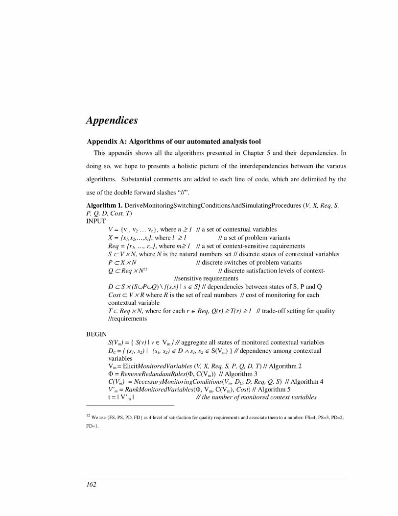
162
Appendices
68 Appendix A: Algorithms of our automated analysis tool
This appendix shows all the algorithms presented in Chapter 5 and their dependencies. In
doing so, we hope to presents a holistic picture of the interdependencies between the various
algorithms. Substantial comments are added to each line of code, which are delimited by the
use of the double forward slashes “//”.
Algorithm 1. DeriveMonitoringSwitchingConditionsAndSimulatingProcedures (V, X, Req, S, P, Q, D, Cost, T) INPUT
V = {v1, v2 … vn}, where n ' 1 // a set of contextual variables
X = {x1,x2,…,xl}, where l ' 1 // a set of problem variants
Req = {r1, …, rm}, where m' 1 // a set of context-sensitive requirements S " V & N, where N is the natural numbers set // discrete states of contextual variables
P " X & N // discrete switches of problem variants
Q " Req & N12 // discrete satisfaction levels of context-//sensitive requirements
D " S & (S#P#Q) \ {(s,s) | s ( S} // dependencies between states of S, P and Q
Cost " V & R where R is the set of real numbers // cost of monitoring for each contextual variable
T " Req & N, where for each r ( Req, Q(r) ' T(r) ' 1 // trade-off setting for quality //requirements
BEGIN
S(Vm) = { S(v) | v ( Vm } // aggregate all states of monitored contextual variables
DC = { (s1, s2) |
(s1, s2) ( D * s1, s2 ( S(Vm) } // dependency among contextual variables Vm = ElicitMonitoredVariables (V, X, Req, S, P, Q, D, T) // Algorithm 2 = RemoveRedundantRules(, C(Vm)) // Algorithm 3
C(Vm) = NecessaryMonitoringConditions(Vm, DC, D, Req, Q, S) // Algorithm 4 V’m = RankMonitoredVariables(, Vm, C(Vm), Cost) // Algorithm 5 t = | V’m | // the number of monitored context variables
12 We use {FS, PS, PD, FD} as 4 level of satisfaction for quality requirements and associate them to a number: FS=4, PS=3, PD=2,
FD=1.
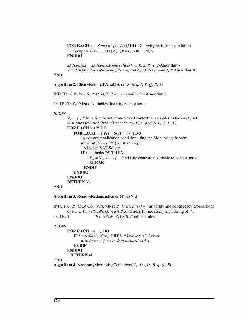
163
FOR EACH x ( X and p([1.. P(x)] DO //deriving switching conditions
C(x=p) = { (s1, ..., st) | (*i=1..t vi=si) * * (x=p)} ENDDO SATcontext = SATcontextGeneration(V’m, X, S, P, ) //Algorithm 7
SimulateMonitoringSwitchingProcedure(Vm’, X, SATcontext) // Algorithm 10 END Algorithm 2. ElicitMonitoredVariables (V, X, Req, S, P, Q, D, T) INPUT: V, X, Req, S, P, Q, D, T // same as defined in Algorithm 1 OUTPUT: Vm // list of variables that may be monitored
BEGIN
Vm = { } // Initialise the set of monitored contextual variables to the empty set = EncodeVariabilityAndDependency (V, X, Req, S, P, Q, D, T)
FOR EACH v (V DO
FOR EACH i, j ([1 .. S(v)] | i % j DO // construct validation condition using the Monitoring theorem
R9 = ( $ v = i) $ (not $ v = j) // invoke SAT-Solver IF satisfiable(R9) THEN
Vm = Vm # {v} // add the contextual variable to be monitored: BREAK
ENDIF ENDDO ENDDO RETURN Vm
END Algorithm 3. RemoveRedundantRules (, C(Vm)) INPUT " ((S#P#Q) & B), where B={true, false} // variability and dependency propositions
C(Vm) " Vm & ((S#P#Q) & B)) // conditions for necessary monitoring of Vm
OUTPUT " ((S#P#Q) & B) // refined rules BEGIN
FOR EACH v ( Vm DO IF ! satisfiable (C(v)) THEN // invoke SAT-Solver = Remove facts in associated with v ENDIF ENDDO
RETURN END Algorithm 4. NecessaryMonitoringConditions(Vm, DC , D, Req, Q , S)
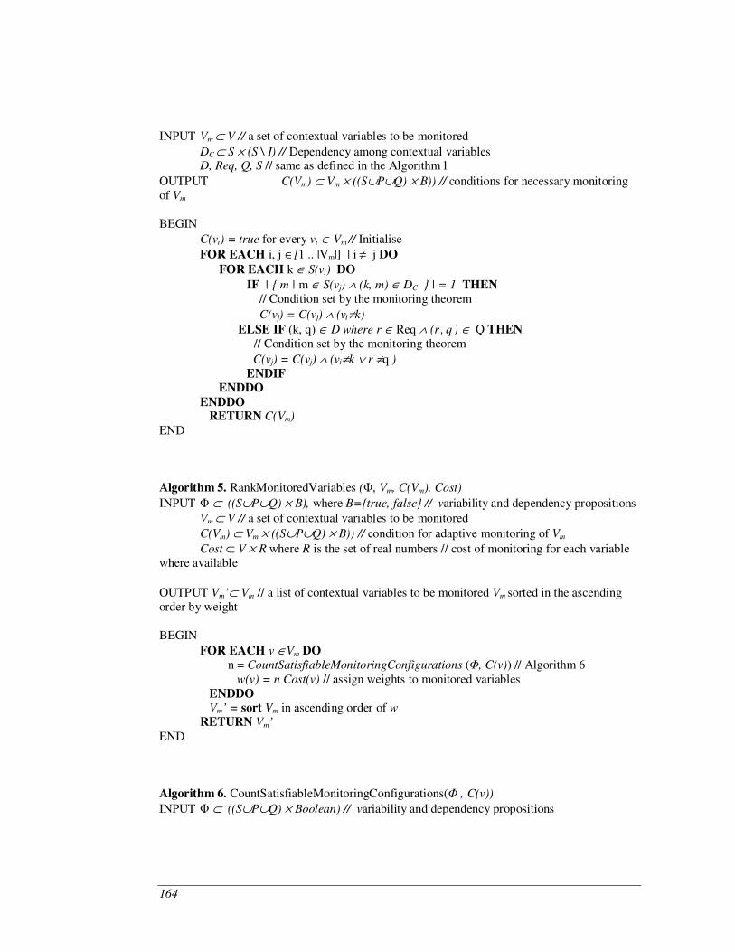
164
INPUT Vm " V // a set of contextual variables to be monitored
DC " S & (S \ I) // Dependency among contextual variables
D, Req, Q, S // same as defined in the Algorithm 1
OUTPUT C(Vm) " Vm & ((S#P#Q) & B)) // conditions for necessary monitoring of Vm
BEGIN
C(vi) = true for every vi ( Vm // Initialise
FOR EACH i, j ([1 .. |Vm|] | i % j DO FOR EACH k ( S(vi) DO
IF | { m | m ( S(vj) * (k, m) ( DC } | = 1 THEN // Condition set by the monitoring theorem
C(vj) = C(vj) * (vi%k)
ELSE IF (k, q) ( D where r ( Req * (r , q ) ( Q THEN // Condition set by the monitoring theorem
C(vj) = C(vj) * (vi%k ) r %q ) ENDIF ENDDO ENDDO
RETURN C(Vm) END Algorithm 5. RankMonitoredVariables (, Vm, C(Vm), Cost)
INPUT " ((S#P#Q) & B), where B={true, false} // variability and dependency propositions Vm " V // a set of contextual variables to be monitored
C(Vm) " Vm & ((S#P#Q) & B)) // condition for adaptive monitoring of Vm
Cost " V & R where R is the set of real numbers // cost of monitoring for each variable where available
OUTPUT Vm’" Vm // a list of contextual variables to be monitored Vm sorted in the ascending order by weight BEGIN
FOR EACH v (Vm DO n = CountSatisfiableMonitoringConfigurations (, C(v)) // Algorithm 6 w(v) = n Cost(v) // assign weights to monitored variables ENDDO Vm’ = sort Vm in ascending order of w RETURN Vm’ END Algorithm 6. CountSatisfiableMonitoringConfigurations( , C(v))
INPUT " ((S#P#Q) & Boolean) // variability and dependency propositions
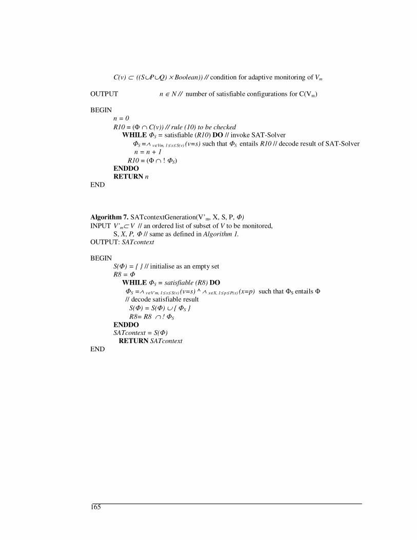
165
C(v) " ((S#P#Q) & Boolean)) // condition for adaptive monitoring of Vm
OUTPUT n ( N // number of satisfiable configurations for C(Vm) BEGIN n = 0
R10 = ( $ C(v)) // rule (10) to be checked WHILE S = satisfiable (R10) DO // invoke SAT-Solver
S =* v(Vm, 1+ s+ S(v) (v=s) such that S entails R10 // decode result of SAT-Solver n = n + 1
R10 = ( $ ! S) ENDDO RETURN n
END Algorithm 7. SATcontextGeneration(V’m, X, S, P, )
INPUT V’m" V // an ordered list of subset of V to be monitored, S, X, P, // same as defined in Algorithm 1. OUTPUT: SATcontext BEGIN
S() = { } // initialise as an empty set R8 =
WHILE S = satisfiable (R8) DO
S =* v(V’m, 1+ s+ S(v) (v=s) ^ * x(X, 1+ p+ P(x) (x=p) such that S entails // decode satisfiable result
S() = S() # { S }
R8= R8 $ ! S ENDDO SATcontext = S() RETURN SATcontext END
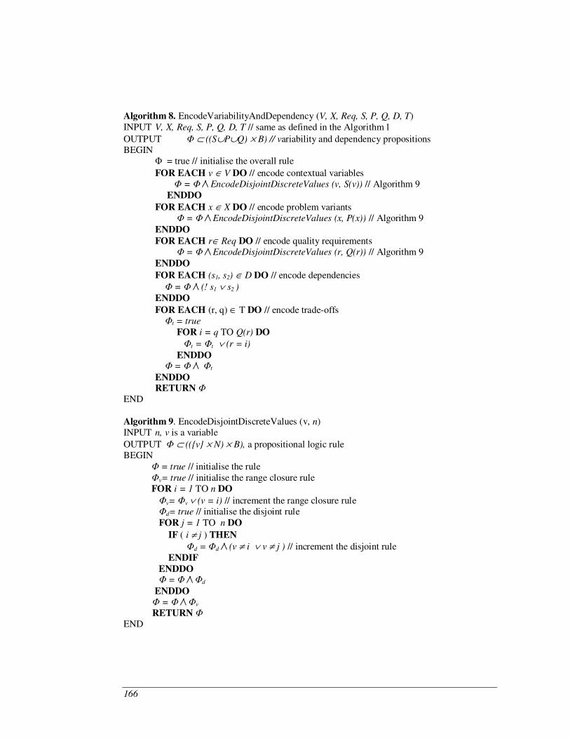
166
Algorithm 8. EncodeVariabilityAndDependency (V, X, Req, S, P, Q, D, T) INPUT V, X, Req, S, P, Q, D, T // same as defined in the Algorithm 1
OUTPUT " ((S#P#Q) & B) // variability and dependency propositions BEGIN = true // initialise the overall rule
FOR EACH v ( V DO // encode contextual variables = /\ EncodeDisjointDiscreteValues (v, S(v)) // Algorithm 9 ENDDO
FOR EACH x ( X DO // encode problem variants = /\ EncodeDisjointDiscreteValues (x, P(x)) // Algorithm 9 ENDDO FOR EACH r( Req DO // encode quality requirements = /\ EncodeDisjointDiscreteValues (r, Q(r)) // Algorithm 9 ENDDO
FOR EACH (s1, s2) ( D DO // encode dependencies = /\ (! s1 ) s2 ) ENDDO
FOR EACH (r, q) ( T DO // encode trade-offs t = true FOR i = q TO Q(r) DO t = t ) (r = i) ENDDO = /\ t ENDDO RETURN END Algorithm 9. EncodeDisjointDiscreteValues (v, n) INPUT n, v is a variable
OUTPUT " (({v} & N) & B), a propositional logic rule BEGIN
= true // initialise the rule v= true // initialise the range closure rule FOR i = 1 TO n DO
v= v ) (v = i) // increment the range closure rule d= true // initialise the disjoint rule FOR j = 1 TO n DO
IF ( i % j ) THEN d = d /\ (v % i ) v % j ) // increment the disjoint rule ENDIF ENDDO = /\ d
ENDDO = /\ v RETURN
END
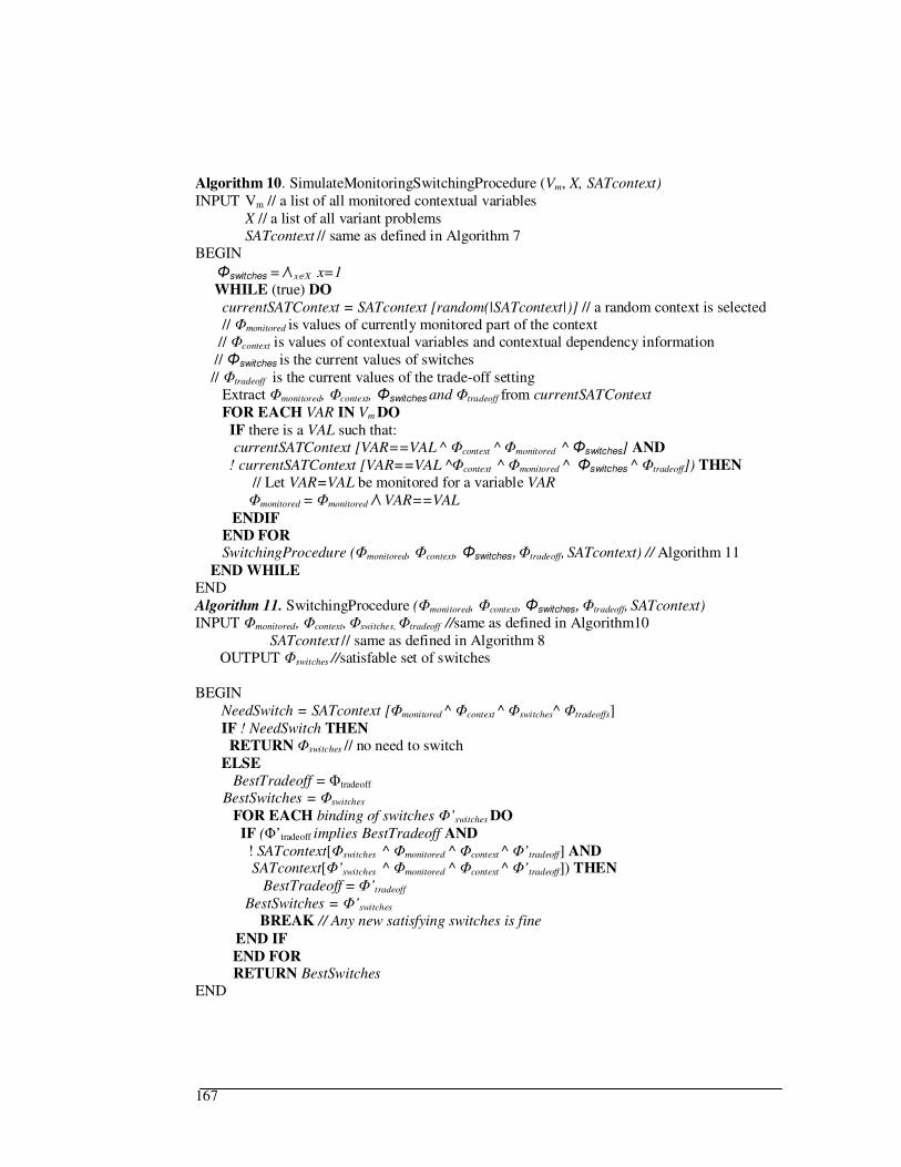
167
Algorithm 10. SimulateMonitoringSwitchingProcedure (Vm, X, SATcontext) INPUT Vm // a list of all monitored contextual variables
X // a list of all variant problems SATcontext // same as defined in Algorithm 7
BEGIN
switches = /\ x(X x=1 WHILE (true) DO currentSATContext = SATcontext [random(|SATcontext|)] // a random context is selected // monitored is values of currently monitored part of the context // context is values of contextual variables and contextual dependency information // switches is the current values of switches // tradeoff is the current values of the trade-off setting Extract monitored, context, switches and tradeoff from currentSATContext FOR EACH VAR IN Vm DO IF there is a VAL such that: currentSATContext [VAR==VAL ^ context ^ monitored ^ switches] AND ! currentSATContext [VAR==VAL ^context ^ monitored ^ switches ^ tradeoff]) THEN // Let VAR=VAL be monitored for a variable VAR monitored = monitored /\ VAR==VAL
ENDIF END FOR SwitchingProcedure (monitored, context, switches, tradeoff, SATcontext) // Algorithm 11 END WHILE END Algorithm 11. SwitchingProcedure (monitored, context, switches, tradeoff, SATcontext) INPUT monitored, context, switches, tradeoff //same as defined in Algorithm10
SATcontext // same as defined in Algorithm 8 OUTPUT switches //satisfable set of switches
BEGIN NeedSwitch = SATcontext [monitored ^ context ^ switches^ tradeoffs] IF ! NeedSwitch THEN RETURN switches // no need to switch ELSE BestTradeoff = tradeoff
BestSwitches = switches FOR EACH binding of switches ’switches DO IF (’tradeoff implies BestTradeoff AND ! SATcontext[switches ^ monitored ^ context ^ ’tradeoff] AND SATcontext[’switches ^ monitored ^ context ^ ’tradeoff]) THEN BestTradeoff = ’tradeoff
BestSwitches = ’switches
BREAK // Any new satisfying switches is fine
END IF END FOR RETURN BestSwitches
END
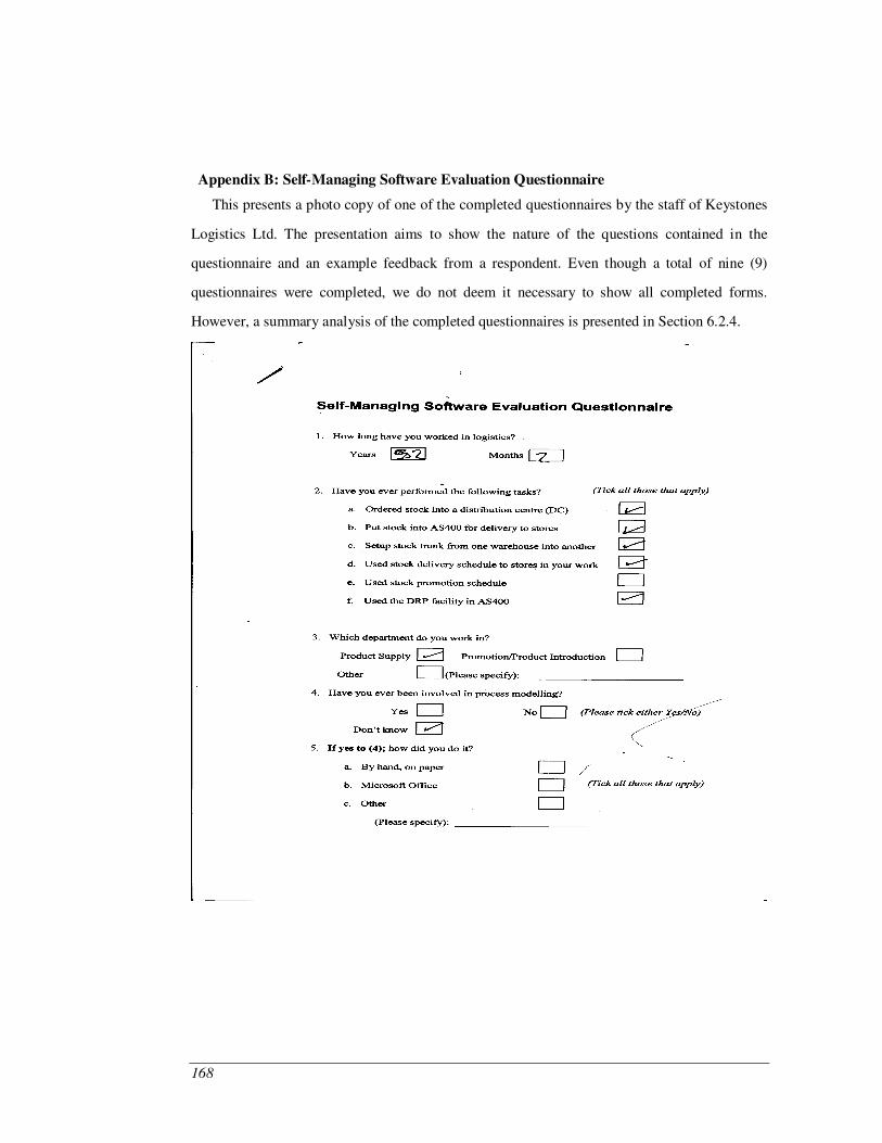
168
Figure 69 Appendix B: Self-Managing Software Evaluation Questionnaire
This presents a photo copy of one of the completed questionnaires by the staff of Keystones
Logistics Ltd. The presentation aims to show the nature of the questions contained in the
questionnaire and an example feedback from a respondent. Even though a total of nine (9)
questionnaires were completed, we do not deem it necessary to show all completed forms.
However, a summary analysis of the completed questionnaires is presented in Section 6.2.4.
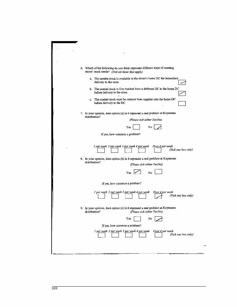
169
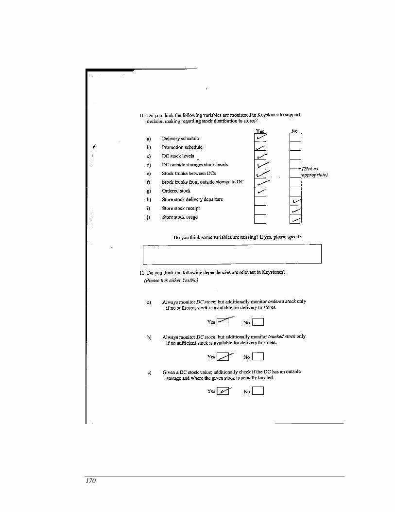
170
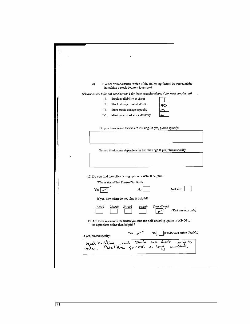
171
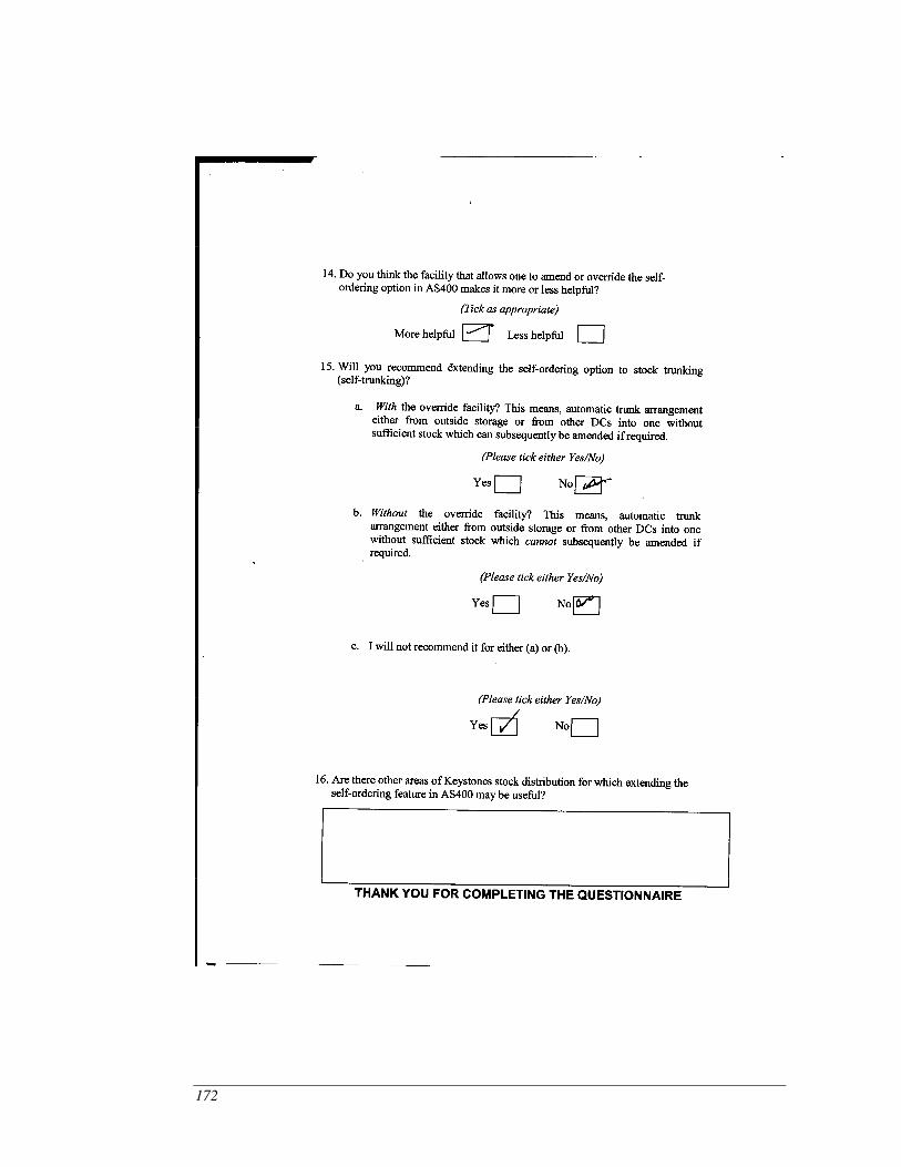
172
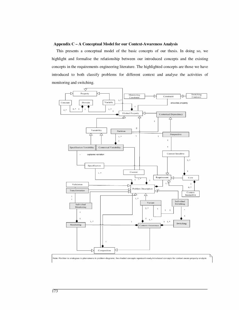
173
Figure 70 Appendix C – A Conceptual Model for our Context-Awareness Analysis
This presents a conceptual model of the basic concepts of our thesis. In doing so, we
highlight and formalise the relationship between our introduced concepts and the existing
concepts in the requirements engineering literature. The highlighted concepts are those we have
introduced to both classify problems for different context and analyse the activities of
monitoring and switching.
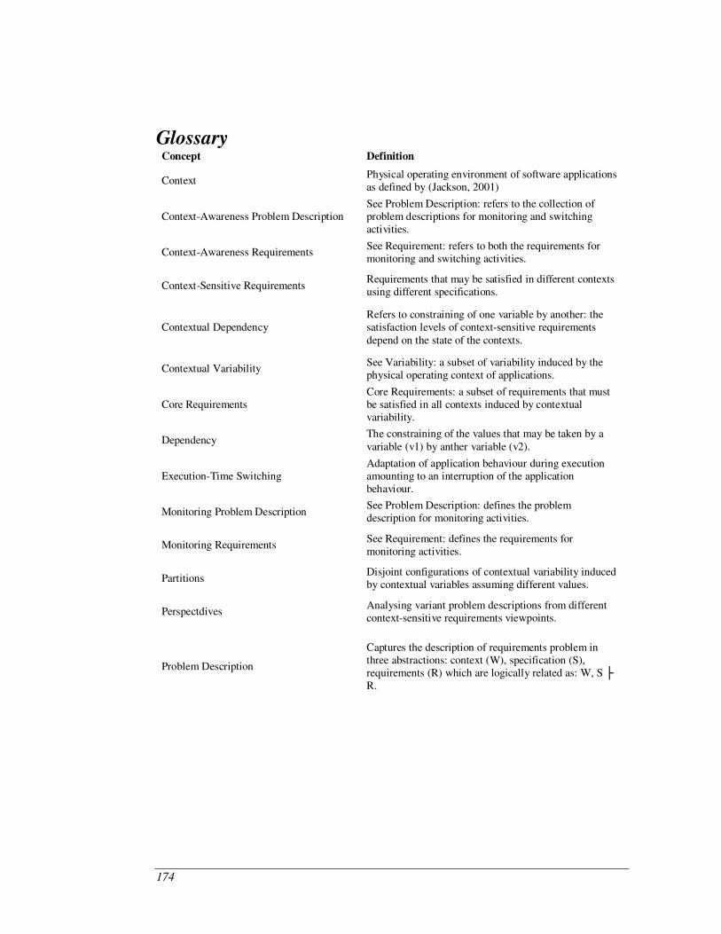
174
Glossary Concept Definition
Context Physical operating environment of software applications as defined by (Jackson, 2001)
Context-Awareness Problem Description See Problem Description: refers to the collection of problem descriptions for monitoring and switching activities.
Context-Awareness Requirements See Requirement: refers to both the requirements for monitoring and switching activities.
Context-Sensitive Requirements Requirements that may be satisfied in different contexts using different specifications.
Contextual Dependency Refers to constraining of one variable by another: the satisfaction levels of context-sensitive requirements depend on the state of the contexts.
Contextual Variability See Variability: a subset of variability induced by the physical operating context of applications.
Core Requirements Core Requirements: a subset of requirements that must be satisfied in all contexts induced by contextual variability.
Dependency The constraining of the values that may be taken by a variable (v1) by anther variable (v2).
Execution-Time Switching Adaptation of application behaviour during execution amounting to an interruption of the application behaviour.
Monitoring Problem Description See Problem Description: defines the problem description for monitoring activities.
Monitoring Requirements See Requirement: defines the requirements for monitoring activities.
Partitions Disjoint configurations of contextual variability induced by contextual variables assuming different values.
Perspectdives Analysing variant problem descriptions from different context-sensitive requirements viewpoints.
Problem Description
Captures the description of requirements problem in three abstractions: context (W), specification (S), requirements (R) which are logically related as: W, S R.
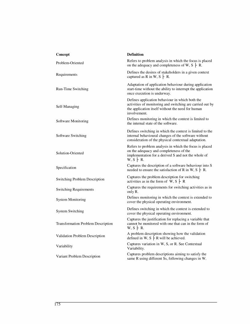
175
Concept Definition
Problem-Oriented Refers to problem analysis in which the focus is placed on the adequacy and completeness of W, S R.
Requirements Defines the desires of stakeholders in a given context captured as R in W, S R.
Run-Time Switching Adaptation of application behaviour during application start-time without the ability to interrupt the application once execution is underway.
Self-Managing
Defines application behaviour in which both the activities of monitoring and switching are carried out by the application itself without the need for human involvement.
Software Monitoring Defines monitoring in which the context is limited to the internal state of the software.
Software Switching Defines switching in which the context is limited to the internal behavioural changes of the software without consideration of the physical contextual adaptation.
Solution-Oriented
Refers to problem analysis in which the focus is placed on the adequacy and completeness of the implementation for a derived S and not the whole of W, S R.
Specification Captures the description of a software behaviour into S needed to ensure the satisfaction of R in W, S R.
Switching Problem Description Captures the problem description for switching activities as in the form of W, S R
Switching Requirements Captures the requirements for switching activities as in only R.
System Monitoring Defines monitoring in which the context is extended to cover the physical operating environment.
System Switching Defines switching in which the context is extended to cover the physical operating environment.
Transformation Problem Description Captures the justification for replacing a variable that cannot be monitored with one that can in the form of W, S R.
Validation Problem Description A problem description showing how the validation defined in W, S R will be achieved.
Variability Captures variation in W, S, or R. See Contextual Variability.
Variant Problem Description Captures problem descriptions aiming to satisfy the same R using different Ss, following changes in W.
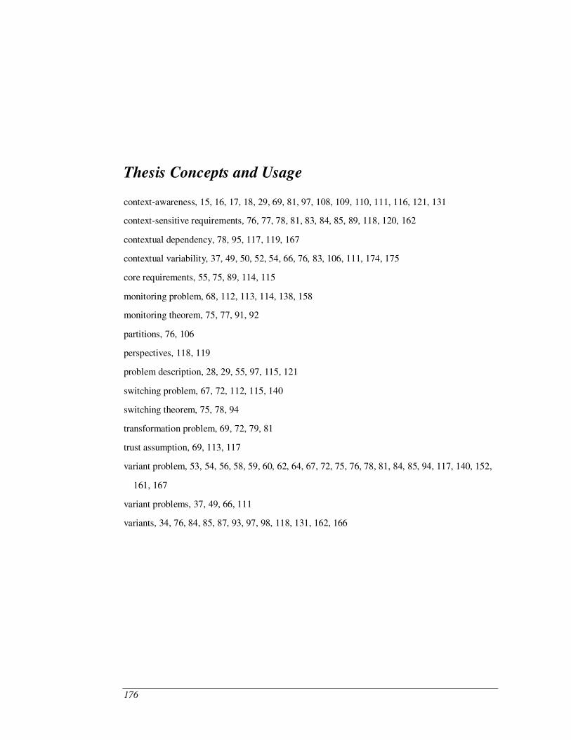
176
Thesis Concepts and Usage
context-awareness, 15, 16, 17, 18, 29, 69, 81, 97, 108, 109, 110, 111, 116, 121, 131
context-sensitive requirements, 76, 77, 78, 81, 83, 84, 85, 89, 118, 120, 162
contextual dependency, 78, 95, 117, 119, 167
contextual variability, 37, 49, 50, 52, 54, 66, 76, 83, 106, 111, 174, 175
core requirements, 55, 75, 89, 114, 115
monitoring problem, 68, 112, 113, 114, 138, 158
monitoring theorem, 75, 77, 91, 92
partitions, 76, 106
perspectives, 118, 119
problem description, 28, 29, 55, 97, 115, 121
switching problem, 67, 72, 112, 115, 140
switching theorem, 75, 78, 94
transformation problem, 69, 72, 79, 81
trust assumption, 69, 113, 117
variant problem, 53, 54, 56, 58, 59, 60, 62, 64, 67, 72, 75, 76, 78, 81, 84, 85, 94, 117, 140, 152,
161, 167
variant problems, 37, 49, 66, 111
variants, 34, 76, 84, 85, 87, 93, 97, 98, 118, 131, 162, 166
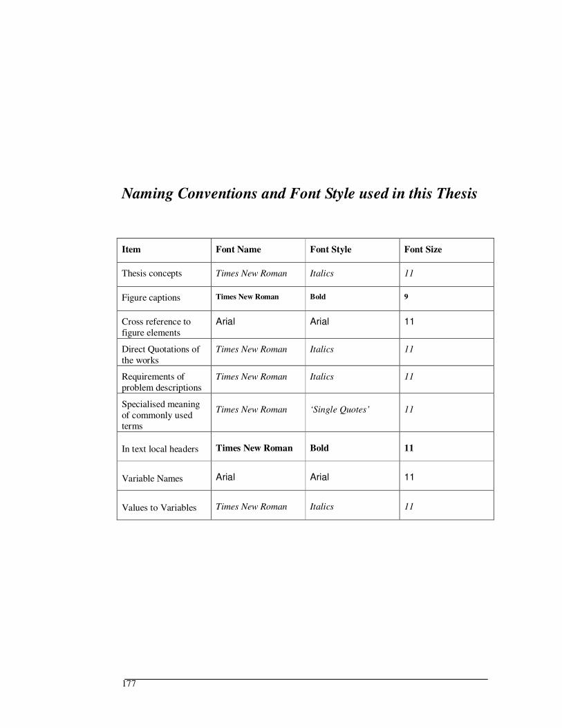
177
Naming Conventions and Font Style used in this Thesis
Item Font Name Font Style Font Size
Thesis concepts Times New Roman Italics 11
Figure captions Times New Roman Bold 9
Cross reference to figure elements
Arial Arial 11
Direct Quotations of the works
Times New Roman Italics 11
Requirements of problem descriptions
Times New Roman Italics 11
Specialised meaning of commonly used terms
Times New Roman ‘Single Quotes’ 11
In text local headers Times New Roman Bold 11
Variable Names Arial Arial 11
Values to Variables Times New Roman Italics 11
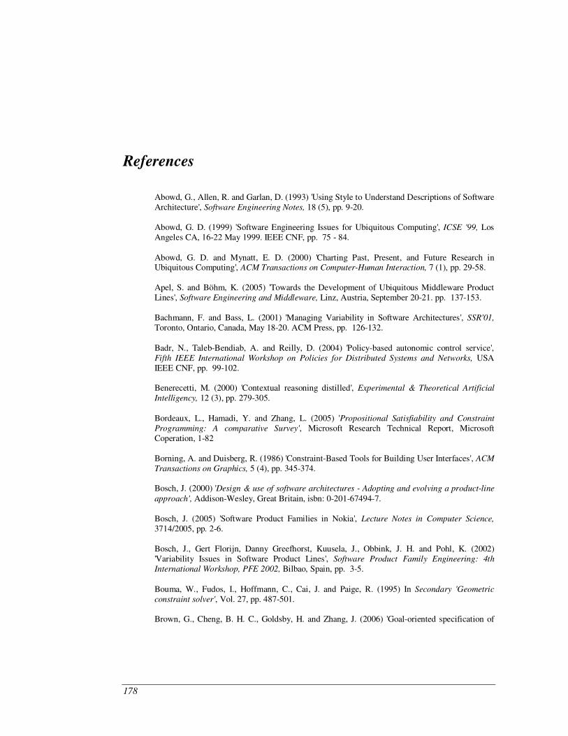
178
References
Abowd, G., Allen, R. and Garlan, D. (1993) 'Using Style to Understand Descriptions of Software Architecture', Software Engineering Notes, 18 (5), pp. 9-20.
Abowd, G. D. (1999) 'Software Engineering Issues for Ubiquitous Computing', ICSE '99, Los Angeles CA, 16-22 May 1999. IEEE CNF, pp. 75 - 84.
Abowd, G. D. and Mynatt, E. D. (2000) 'Charting Past, Present, and Future Research in Ubiquitous Computing', ACM Transactions on Computer-Human Interaction, 7 (1), pp. 29-58.
Apel, S. and Böhm, K. (2005) 'Towards the Development of Ubiquitous Middleware Product Lines', Software Engineering and Middleware, Linz, Austria, September 20-21. pp. 137-153.
Bachmann, F. and Bass, L. (2001) 'Managing Variability in Software Architectures', SSR'01, Toronto, Ontario, Canada, May 18-20. ACM Press, pp. 126-132.
Badr, N., Taleb-Bendiab, A. and Reilly, D. (2004) 'Policy-based autonomic control service', Fifth IEEE International Workshop on Policies for Distributed Systems and Networks, USA IEEE CNF, pp. 99-102.
Benerecetti, M. (2000) 'Contextual reasoning distilled', Experimental & Theoretical Artificial Intelligency, 12 (3), pp. 279-305.
Bordeaux, L., Hamadi, Y. and Zhang, L. (2005) 'Propositional Satisfiability and Constraint Programming: A comparative Survey', Microsoft Research Technical Report, Microsoft Coperation, 1-82
Borning, A. and Duisberg, R. (1986) 'Constraint-Based Tools for Building User Interfaces', ACM Transactions on Graphics, 5 (4), pp. 345-374.
Bosch, J. (2000) 'Design & use of software architectures - Adopting and evolving a product-line approach', Addison-Wesley, Great Britain, isbn: 0-201-67494-7.
Bosch, J. (2005) 'Software Product Families in Nokia', Lecture Notes in Computer Science, 3714/2005, pp. 2-6.
Bosch, J., Gert Florijn, Danny Greefhorst, Kuusela, J., Obbink, J. H. and Pohl, K. (2002) 'Variability Issues in Software Product Lines', Software Product Family Engineering: 4th International Workshop, PFE 2002, Bilbao, Spain, pp. 3-5.
Bouma, W., Fudos, I., Hoffmann, C., Cai, J. and Paige, R. (1995) In Secondary 'Geometric constraint solver', Vol. 27, pp. 487-501.
Brown, G., Cheng, B. H. C., Goldsby, H. and Zhang, J. (2006) 'Goal-oriented specification of

References
179
adaptation requirements engineering in adaptive systems', SEAMS at ICSE, US ACM Press New York, NY, USA, pp. 23-29.
Buchanan, B. G. (1984) 'Rule-based expert systems', Addison-Wesley Longman Publishing Co., Inc, Boston, MA, USA, isbn: 0201101726.
Bühne, S., Halmans, G. and Pohl, K. (2003) 'Modelling Dependencies between Variation Points in Use Case Diagrams', Proceedings of the 9th International Workshop on Requirements Engineering Foundation for Software Quality (REFSQ), Klagenfurt, Austria, pp. 1-12.
Campbell, A. and Alexander, M. (1997) 'What’s wrong with strategy', Harvard Business Review, 75 (6), pp. 42-51.
Card, S. K., Moran, T. P. and Newell, A. (1983) 'The Psychology of Human-computer Interaction', Lawrence Erlbaum Associates, isbn: 9780898598699.
Carlsson, M., Ottosson, G. and Carlson, B. (1997) In Secondary 'An open-ended finite domain constraint solver', Vol. 1292 Springer, pp. 191–206.
Castro, J., Kolp, M. and Mylopoulos, J. (2002) 'Towards requirements-driven information systems engineering: the Tropos project', Information Systems, 27 (6), pp. 365-389.
Chandra, S. and Bhattaram, S. (2003) 'Patterns Approach to Building Software Systems', International Conference on Software Engineering 2003 (ICSE'03), Portland, Oregon, USA, May 9. pp. 1-3.
Chen, G. and Kotz, D. (2000) 'A Survey of Context-Aware Mobile Computing Research', Technical Report, Dartmouth Computer Science, 1-16
Cheng, B. H. C. and Atlee, J. M. (2007) 'Research Directions in Requirements Engineering', IEEE International Conference on Software Engineering IEEE Computer Society Washington, DC, USA, pp. 285-303.
Cheng, S. W., Garlan, D. and Schmerl, B. (2006) 'Architecture-based self-adaptation in the presence of multiple objectives', SEAMS at ICSE ACM Press New York, NY, USA, pp. 2-8.
Chung, L., Nixon, B. A., Yu, E. and Mylopoulos, J. (2000) 'Non-Functional Requirements in software engineering', (2000 Edn), Kluwer Academic Publishers, Norwell, Massachusetts, London, Boston, Dorderecht, isbn: 0-7923-8666-3.
Classen, A., Heymans, P., Laney, R., Nuseibeh, B. and Tun, T. (2007) 'On the Structure of Problem Variability:From Feature Diagrams to Problem Frames', 1st -VaMoS, Limerick, Ireland, January 16–18, 2007. Lero, Limerick, pp. 110-117.
Claycamp, H. J. and Massy, W. F. (1968) 'A Theory of Market Segmentation', Journal of Marketing Research, 5 (4), pp. 388-394.
Coatta, T. and Neufeld, G. (1994) 'Distributed Configuration Management Using Composite Objects and Constraints', Distributed Systems Engineering, Distrib. Systems Engineering. (1), pp. 294-303.
Cockburn, A. (2001) 'Writing effective use cases', (1st Edn), Addison-Wesley, Longman, Upper Saddle River, NJ, isbn: 0201702258.
References
180
Cohen, D., Feather, M. S., Narayanaswamy, K. and Fickas, S. S. (1997) 'Automatic Monitoring of Software Requirements', Software Engineering IEEE CNF, pp. 602-603.
Cousin, L. and Collofello, J. S. (1992) 'A task-based approach to improving the software maintenance process', Software Maintenance, pp. 118-126.
Dardenne, A., van Lamsweerde, A. and Fickas, S. (1993) 'Goal-directed requirements acquisition', Selected Papers of the Sixth International Workshop on Software Specification and Design table of contents, 20, pp. 3-50.
Dickson, P. R. and Ginter, J. L. (1987) 'Market Segmentation, Product Differentiation, and Marketing Strategy', Journal of Marketing, 51 (2), pp. 1-10.
Dourish, P. (2004) 'What we talk about when we talk about context', Ubiquitous Computing Springer, pp. 19-30.
Easterbrook, S. and Sim, S. E. (2006) 'Case Studies for Software Engineers: Tutorial F2', ICSE, pp. 1-82.
Faulk, S. R. (2001) 'Product-line requirements specification (PRS): an approach and case study', 5th IEEE International Symposium on Requirements Engineering IEEE CNF, pp. 48-55.
Feather, M., Fickas, S., Van Lamsweerde, A. and Ponsard, C. (1998) 'Reconciling System Requirements and Runtime Behavior', Proceedings of the 9th International Workshop on Software Specification and Design, DC, USA IEEE CNF, pp. 50-59.
Fickas, S. and Feather, M. (1995) 'Requirements Monitoring in Dynamic Environments', Proceedings of the Second IEEE International Symposium on Requirements Engineering, pp. 140-147.
Fillmore, C. J. (1967) In Secondary 'The Case for Case'(Eds) Bach and Harms) New York: Holt, Rinehart, and Winston, pp. 1-88,.
Fowler, M. (1997) 'Analysis Patterns: Reusable Object Models', Addison-Wesley Publishing Company, United States of America, isbn: 0-101-89542-0.
Frakes, W., Prieto, Diaz, R. and Fox, C. (1998) 'DARE: Domain analysis and reuse environment', Annals of Software Engineering, 5, pp. 125-141.
Georgiadis, I., Magee, J. and Kramer, J. (2002) 'Self-Organising Software Architectures for Distributed Systems', ACM SIGSOFT Workshop on Self-Healing Systems (WOSS ‘02), Charleston, South Carolina, November 18, 2002. ACM, pp. 33-38.
Gomaa, H. and Hussein, M. (2004a) 'Dynamic Software Reconfiguration in Software Product Families', Lecture Notes in Computer Science, 3014/2004, pp. 435 - 444.
Gomaa, H. and Hussein, M. (2004b) 'Software Reconfiguration Patterns for Dynamic Evolution of Software Architectures', Proceedings of the Fourth Working IEEE/IFIP Conference on Software Architecture (WICSA’04) IEEE CNF, pp. 1-10.
Grimm, R., Davis, J., Hendrickson, B., Lemar, E., MacBeth, A., Swanson, S., Anderson, T., Bershad, B. and Borriello, G. (2001) 'Systems Directions for Pervasive Computing', Proceedings
References
181
of the 8th Workshop on Hot Topics in Operating Systems (HotOS-VIII), Elmau, Germany, May 2001, pp. 147-151.
Grimm, R., Davis, J., Lemar, E., Macbeth, A., Swanson, S., Anderson, T., Bershad, B., Borriello, G., Gribble, S. and Wetherall, D. (2004) 'System Support for Pervasive Applications', ACM Transactions on Computer Systems., 22 (4), pp. 421–486.
Haban, D. and Wybranietz, D. (1990) 'A hybrid monitor for behavior and performance analysis ofdistributed systems', Transactions on Software Enginnering, 16 (2), pp. 197-211.
Haley, C. B., Laney, R. C., Moffett, J. D. and Nuseibeh, B. (2006) 'Using trust assumptions with security requirements', Requirements Engineering, 11 (2), pp. 138-151.
Hall, J. G., Rapanotti, L. and Jackson, M. (2007) 'Problem Oriented Software Engineering: A design-theoretic framework for software engineering', 5th International Conference on Software Engineering and Formal Methods, pp. 15-24.
Hall, J. G., Rapanotti, L. and Jackson, M. A. (2008) 'Problem Oriented Software Engineering: Solving the Package Router Control Problem', IEEE Transactions on Software Engineering, 34 (2), pp. 226-241.
Hallsteinsen, S., Fægri, T. E. and Syrstad, M. (2004) 'Patterns in Product Family Architecture Design', Lecture Notes in Computer Science, 3014/2004, pp. 261 - 268.
Harrison, B. (2005) 'Service-oriented architectures and AOSD', AOSD-Europe Workshop, Glasgow, UK, 24 July 2005. pp.
Harter, A., Hopper, A., Steggles, P., Ward, A. and Webster, P. (2002) 'The Anatomy of a Context-Aware Application', Wireless Networks, 8 (2-3), pp. 187 - 197.
Henderson, P. (2000) 'Systems Engineering for Business Process Change: Collected Papers from the Epsrc Research Programme', Springer, isbn: 1852332220.
Hinchey, M. G. and Sterritt, R. (2006) 'Self-Managed Systems', IEEE Software, 39 (2), pp. 107 - 109
Hofmann, R., Klar, R., Mohr, B., Quick, A. and Siegle, M. (1994) 'Distributed performance monitoring: methods, tools, andapplications', Transactions on Software Enginnering, 5 (6), pp. 585-598.
Hollan, J., Hutchins, E. and Kirsh, D. (2000) In Secondary 'Distributed cognition: toward a new foundation for human-computer interaction research', Vol. 7 ACM Press New York, NY, USA, pp. 174-196.
Hui, B., Liaskos, S. and Mylopoulos, J. (2003) 'Requirements analysis for customizable software: a goals-skills-preferences framework', 11th Internation Conference on Software Requirements Enginnering IEEE CNF, pp. 117-126.
ICSE, S. c.-l. w. (2006) In Secondary 'ICSE Workshop on Software Engineering for Adaptive and Self-Managing Systems (SEAMS)'url: http://www.cse.msu.edu/SEAMS/cfpSEAMS2006.html.
References
182
Ivan Jureta, John Mylopoulos and Faulkner, S. (2008) In Secondary 'Revisiting the Core Ontology and Problems in Requirements Enginnering' IEEE CNF, Barcelona, Spain.
Jackson, M. (2001) 'Problem Frames: Analyzing and structuring software development problems', (1st Edn), Addison-Wesley, New York, Oxford, isbn: 0-201-59267-X.
Janik, A. and Zielinski, K. (2006) 'Transparent resource management and self-adaptability using multitasking virtual machine RM API', SEAMS at ICSE ACM Press New York, NY, USA, pp. 51-57.
Jaring, M., Krikharr, R. L. and Bosch, J. (2004) 'Representing variabilities in a family of MRI scanners', Software-Practice And Experiance, 34, pp. 69-100.
Jessor, R. and Shweder, R. A. (1996) 'Ethnography and Human Development: Context and Meaning in Social Inquiry', University Of Chicago Press, isbn: 0226399036.
Keepence, B. and Mannion, M. (1999) 'Using Patterns to Model Variabilities in Product Families', IEEE Software, July-August. IEEE Press, pp. 102-107.
Kephart, J. O. and Chess, D. M. (2003) 'The vision of autonomic computing', Computer, 36 (1), pp. 41-50.
Kim, M., Jeong, J. and Park, S. (2005) 'From Product Lines to Self-Managed Systems: An Architecture-Based Runtime Reconfiguration Framework', Workshop on the Design and Evolution of Autonomic Application Software (DEAS 2005 ACM Press, pp. 1-7.
Kindberg, T. and Fox, A. (2002) 'System Software for Ubiquitous Computing', Pervasive Computing, pp. 70-80.
Kramer, J. and Magee, J. (1990) 'The evolving philosophers problem: dynamic change management', IEEE Transactions on Software Engineering, 16 (11).
Kramer, J. and Magee, J. (2007) 'Self-Managed Systems: an Architectural Challenge', International Conference on Software Engineering, May. pp. 259-268.
Lapouchnian, A., Yu, Y., Liaskos, S. and Mylopoulos, J. (2006) 'Requirements-Driven Design of Autonomic Application Software', CASCON2006, Canada, pp. 1-14.
Le Berre, D. (2006) In Secondary 'SAT4J: A satisfiability library for Java'URL http://www. sat4j. org/, Jan, 2006.
Liaskos, S., Jiang, L., Lapouchnian, A., Wang, Y., Yu, Y., Leite, J. C. S. d. P. and Mylopouls, J. (2007) 'Exploring the Dimensions of Variability: a Requirements Engineering Perspective', VaMoS' 07, Limerick, Ireland, pp. 18-26.
Liaskos, S., Lapouchnian, A., Yu, Y., Yu, E. and Mylopoulos, J. (2006) 'On Goal-based Variability Acquisition and Analysis', 14th IEEE International Requirements Engineering Conference (RE'06), Minneapolis/St. Paul, Minnesota, USA,, 11-15 Sept. IEEE CNF, pp. 76 - 85.
Maccari, A. and Heie, A. (2005) 'Managing infinite variability in mobile terminal software', Software - Practice and Experiance, 35 (6), pp. 513–53.
References
183
Magee, J. and Maibaum, T. (2006) 'Towards specification, modelling and analysis of fault tolerance in self managed systems', SEAMS at ICSE ACM Press New York, NY, USA, pp. 30-36.
Mannion, M., Lewis, O., Kaindl, H., Montroni, G. and Wheadon, J. (2000) 'Representing Requirements on Generic Software in an Application Family Model', ICSR Springer-Verlag, pp. 153-169.
Mansouri-Samani, M. and Sloman, M. (1993) 'Monitoring distributed systems', Monitoring Distributed Systems, 7 (6), pp. 20-30.
Mayhew, D. J. (1991) 'Principles and guidelines in software user interface design', Prentice-Hall, Inc. Upper Saddle River, NJ, USA, isbn: 0-13-721929-6.
McDermott, J. (1980) 'R1: A Rule-Based Configurer of Computer Systems', DTIC Research Report ADA223957,
Mckinley, P. K., Sadjadi, S. M., Kasten, E. P. and Cheng, B. H. C. (2004a) 'Composing Adaptive Software', IEEE Computer, 37 (7), pp. 56-64.
McKinley, P. K., Sadjadi, S. M., P.Kasten, E. and Cheng, B. H. C. (2004b) 'Composing Adaptive Software', Computer, pp. 56-64.
Meister, ü., Information, C., Reussner, R., Information, C. and Rohde, M. (2004) 'Managing Product Line Variability by Patterns', Lecture Notes in Computer Science, Erfurt, Germany, September 27-30, 2004. Springer Berlin / Heidelberg, pp. 153.
Metzger, A., Pohl, K., Heymans, P., Schobbens, P. Y. and Saval, G. (2007) 'Disambiguating the Documentation of Variability in Software Product Lines: A Separation of Concerns, Formalization and Automated Analysis', 15th IEEE International Conference on Requirement Engineering, pp. 243-253.
Moorthy, K. S. (1984) 'Market Segmentation, Self-Selection, and Product Line Design', Marketing Science, 3 (4), pp. 288-307.
Nokia (2005) In Secondary 'Nokia Architecture - Platform Architectures'Nokia - http://europe.nokia.com/nokia/0,,62611,00.html, Online, pp. 1-2.
Nokia, F. (2006) In Secondary 'Enterprise: Developing End-To-End Systems', Vol. 1 Nokia Forum, Online, pp. 1-54.
Northrop, L. (2002) 'SEI's software product line tenets', Software IEEE, 19 (4), pp. 32-40.
Nuseibeh, B. (2001) 'Weaving Together Requirements and Architectures', Software Management, 34 (3), pp. 115-117.
Nuseibeh, B. and Easterbrook, S. (2000) 'Requirements engineering: a roadmap', Proceedings of the Conference on The Future of Software Engineering, pp. 35-46.
Ommering, R. V. (2002) 'Building Product Families with Software Components', ICSE 2002, Orlando Florida, USA, pp. 255-265.
References
184
Oreizy, P., Gorlick, M. M., Taylor, R. N., Heimbigner, D., Johnson, G., Nenad Medvidovic, Quilici, A., Rosenblum, D. S. and Wol, A. L. (1999) 'An architecture-based approach to self-adaptive software', Intelligent Systems and Their Applications, 14 (3).
Parnas, D. L. (1976) 'On the Design and Development of Program Families', IEEE Transactions on Software Engineering, 2 (1), pp. 1-9.
Parnas, D. L. (1979) 'Designing software for ease of extension and contraction', IEEE Transactions on Software Engineering, 5 (2), pp. 128 - 138.
Perry, D. E. (1998) 'Generic Architecture Descriptions for Product Lines', Lecture Notes in Computer Science Springer Berlin / Heidelberg, pp. 51 - 56
Peters, D. K. (2000) 'Deriving Real-Time Monitors from System Requirements Documentation', McMaster University, isbn: 0-612-66288-8.
Peters, D. K. and Parnas, D. L. (1998) 'Using test oracles generated from program documentation', Transactions on Software Enginnering, 24 (3), pp. 161-173.
Peters, D. K. and Parnas, D. L. (2002) 'Requirements-based monitors for real-time systems', Software Engineering, IEEE Transactions on, 28 (2), pp. 146-158.
Phalp, K. T., Henderson, P., Walters, R. J. and Abeysinghe, G. (1998) 'RolEnact: role-based enactable models of business processes', Information And Software Technology, 40 (3), pp. 123-133.
Pinto, J. A. (1993) Temporal Reasoning in the Situation Calculus - PhD Thesis, University of Toronto, Toronto
PMI (2004) 'A Guide to the Project Management Body of Knowledge', (3 Edn), isbn: 99-001-2004.
Poladian, V., Sousa, J. P., Garlan, D. and Shaw, M. (2004) 'Dynamic Configuration of Resource-Aware Services', Proceedings of the 26th International Conference on Software Engineering ICSE '04 IEEE Computer Society, pp. 604- 613.
Rajasree, M. S., Reddy, P. J. K. and Janakiram, D. (2003) 'Pattern Oriented Software Development: Moving Seamlessly from Requirements to Architecture', Straw03: International Conference on Software Engineering 2003 (ICSE'03), Portland, Oregon, USA., pp. 1-7.
Robinson, W. (2002) 'Monitoring Software Requirements using Instrumented Code', Proc. of the Hawaii Int. Conf. on Systems Sciences, pp. 3967- 3976.
Robinson, W. (2005) 'Implementing Rule-based Monitors within a Framework for Continuous Requirements Monitoring, best paper nominee', Hawaii International Conference On System Sciences (HICSS'05), Big Island, Hawaii, USA IEEE, pp. 1-8.
Robinson, W. (2006) 'A requirements monitoring framework for enterprise systems', Requirements Engineering, 11 (1), pp. 17-41.
Robinson, W. and Pawlowski, S. (1999) 'Managing requirements inconsistency with development goal monitors', Software Engineering, IEEE Transactions on, 25 (6), pp. 816-835.
References
185
Rozanski, N. and Woods, E. (2005) 'Software Systems Architecture', Addison-Wesley Profession, London, isbn: 0321112296.
Salifu, M., Nuseibeh, B. and Rapanotti, L. (2006) 'Mobile Device Application Pilot Study - Probation Report - Part II', Department of Computing, The Open University, Walton Hall, Milton Keynes, 1-33
Salifu, M., Nuseibeh, B., Rapanotti, L. and Tun, T. T. (2007a) 'Using Problem Descriptions to Represent Variability for Context-Aware Application', First International Workshop on Variability Modelling of Software-Intensive Systems, Limerick, Ireland, January 16th - 18th. Lero, pp. 149-156.
Salifu, M., Nuseibeh, B. and Yu, Y. (2007b) 'Specifying Monitoring and Switching Problems in Context', 15th IEEE International Requirements Engineering Conference, Delhi, India., October 15-19th. pp. 211-220.
Salvador, T., Barile, S. and Sherry, J. (2004) 'Ubiquitous Computing Design Principles: Supporting Human-Human and Human-Computer Transactions', CHI 2004- Late Breaking Results Paper, Vienna, Austria, pp. 24-29.
Sannella, M. (1992) 'The SkyBlue constraint solver', Techi~ ical Report, pp. 92-07.
Scheer, A. W. (1994) 'Business Process Engineering: Reference Models for Industrial Enterprises', Springer-Verlag New York, Inc. Secaucus, NJ, USA, isbn: 3540582347.
Schobbens, P. Y., Heymans, P. and Trigaux, J. C. (2006) 'Feature Diagrams: A Survey and a Formal Semantics', Requirements Engineering Conference IEEE Computer Society Washington, DC, USA, pp. 136-145.
Shneiderman, B. (1992) 'Designing the user interface: strategies for effective human-computer interaction', Addison-Wesley Longman Publishing Co., Inc. Boston, MA, USA, isbn: 0321197860.
Sinnema, M., Deelstra, S., Nijhuis, J. and Bosch, J. (2006) 'Modeling Dependencies in Product Families with COVAMOF', Proceedings of the 13th Annual IEEE International Symposium and Workshop on Engineering of Computer Based Systems (ECBS’06) IEEE CNF, pp. 197-213.
Sochos, P., Ilka Philippow and Riebisch, M. (2004) 'Feature-Oriented Development of Software Product Lines: Mapping Feature Models to the Architecture"', 5th Annual International Conference on Object-Oriented and Internet-based Technologies, Concepts, and Applications for a Networked World (Net.ObjectDays'2004). pp. 138-152.
Sutcliffe, A. (1998) 'The Domain Theory for Requirements Engineering', IEEE Transactions on Software Engineering, 24 (3), pp. 174-196.
Sutcliffe, A., Fickas, S. and M., S. M. (2005) 'Personal and Contextual Requirements Engineering', Requirements Engineering Conference, pp. 19-30.
Sutcliffe, A. G., Maiden, N. A. M., Minocha, S. and Manuel, D. (1998) 'Supporting Scenario-Based Requirements Engineering', IEEE Transactions on Software Engineering, 24 (12).
References
186
Svahnberg, M., Gurp, J. v. and Bosch, J. (2005) 'A taxonomy of variability realization techniques', Software: Practice and Experience, 35 (8), pp. 705-754.
van-Gurp, J., Bosch, J. and Svahnberg, M. (2000) 'Managing Variability in Software Product Lines', Proceedings of IEEE/IFIP Conference on Software Architecture, pp. 45-54.
van der Hoek, A. (1999) 'Configurable Software Architecture in Support of Configuration Management and Software Deployment', International Conference on Software Engineering, pp. 732 - 733.
Van Lamsweerde, A. (2002) 'Goal-oriented requirements engineering: a guided tour', Requirements Engineering Conference, 27-31 Aug. 2001. pp. 249 - 262.
Van Lamsweerde, A., Darimont, R. and Massonet, P. (1995) 'Goal-directed elaboration of requirements for a meeting scheduler: problems and lessons learnt', Proceedings of the Second IEEE International Symposium on, 27-29 Mar 1995. pp. 194-203.
Wang, Y., McIlraith, S. A., Yu, Y. and Mylopoulos, J. (2007) 'An automated approach to monitoring and diagnosing requirements', ACM New York, NY, USA, pp. 293-302.
Wang;, Y., Sheila A. Mcllraith, Yijun Yu and Mylopoulos, J. (2007) 'An Automated Approach to Monitoring and Diagnosing Requirements', IEEE Automated Software Engineering, pp. 293-302.
Want, R., Schilit, B. N., Adams, N. I., Gold, R., Petersen, K., Goldberg, D., Ellis, J. R. and Weiser, M. (1995) 'An Overview of the ParcTab Ubiquitous Computing Experiment', IEEE Personal Communications, pp. 28--43.
Weiser, M. (1993a) 'Some Computer Science Issues in Ubiquitous Computing', Communications of the ACM, pp. 75 - 84.
Weiser, M. (1993b) 'Ubiquitous Computing', Variation of the article below appeared in IEEE Computer "Hot Topics", October 1993., pp. August 16, 1993.
Winbladh, K., Alspaugh, T. A., Ziv, H. and Richardson, D. J. (2006) 'An Automated Approach for Goal-driven, Specification-based Testing', IEEE Automated Software Engineering IEEE CNF, pp. 289-292.
Yu, E. S. K. (1997) 'Towards modelling and reasoning support for early-phaserequirements engineering', Third International Symposium on Requirements Engineering, Washington DC, US, pp. 226-235.
Zave, P. and Jackson, M. (1997) 'Four Dark Corners of Requirements Engineering', ACM Transactions on Software Engineering and Methodology, 6 (1), pp. 1-30.
Zhang, J. and Cheng, B. H. C. (2006a) In Secondary 'Model-based development of dynamically adaptive software'ACM Press New York, NY, USA, pp. 371-380.
Zhang, J. and Cheng, B. H. C. (2006b) 'Using Temporal Logic to Specify Adaptive Program Semantics', Architecting Dependable Systems-Journal of Systems and Software (JSS), 79 (10), pp. 1361-1369.