Embed Size (px)
Citation preview

Faculty of Civil Engineering Institute of Construction Informatics
Analysing trajectories and moments of a one-arm robot to
pick up sheet metals and assemble a shell structure
Analyse von Trajektorien und Lastzuständen eines Ein-Arm-
Roboters zur Montage von dünnwandigen Fassadenstrukturen
By
Khashayar Samiee Moghaddam
from
Islamic Republic of Iran
A Master thesis submitted to the Institute of Construction Informatics, Faculty of Civil Engineer-
ing, Dresden University of Technology in partial fulfilment of the requirements for the
degree of
Master of Science
Responsible Professor: Prof. Dr.-Ing. habil. Karsten Menzel
Second Examiner: Prof. Dr.-Ing. Raimar Scherer
Advisor: Dipl.-Ing. Adrian Schubert
Dresden, 15th June 2020

Analysing trajectories and moments of a one arm robot to Pick up sheet metals and assemble a shell structure Page II
Task Sheet

Analysing trajectories and moments of a one arm robot to Pick up sheet metals and assemble a shell structure Page III
Original Task sheet

Analysing trajectories and moments of a one arm robot to Pick up sheet metals and assemble a shell structure Page IV
Declaration
I confirm that this assignment is my own work and that I have not sought or used the inad-
missible help of third parties to produce this work. I have fully referenced and used inverted
commas for all text directly quoted from a source. Any indirect quotations have been duly
marked as such.
This work has not yet been submitted to another examination institution – neither in Germany
nor outside Germany – neither in the same nor in a similar way and has not yet been pub-
lished.
Dresden,15.06.2020
Place, Date
Signature

Analysing trajectories and moments of a one arm robot to Pick up sheet metals and assemble a shell structure Page V
Acknowledgment
Foremost, I would like to express my sincere gratitude to Prof.Dr.-Ing.habil. Karsten Menzel
for the continuous support of my master thesis, for his patience, motivation, enthusiasm.The
door to Prof. Menzel office was always open whenever I ran into a trouble spot or had a
question about my research or writing.
I would particularly like to single out Dipl.-Ing. Adrian Schubert. I want to thank him for his
excellent cooperation and all the opportunities. The guidance and hints provided by him
served as an invaluable part in the completion of my thesis.
Finally, I must express my very profound gratitude to my parents and to my spouse, whose
love and guidance are with me in whatever I pursue. They support and encourage me
throughout my years of study and through the process of researching and writing this thesis.
This accomplishment would not have been possible without them. Thank you.
Khashayar Samiee Moghaddam
Analysing trajectories and moments of a one arm robot to Pick up sheet metals and assemble a shell structure Page VI
Abstract
The trends in the architecture and construction industry are going forward in the direction of
complex-shaped freeform buildings. The design process of freeform buildings is one chal-
lenge. At the same time, due to lack of flexible construction methods, customized methods
shall be used for the fabrication and construction of those buildings. This may lead to material
loss, high cost, and complex manufacturing and assembly processes.
Shell structures are one of the examples for freeform buildings, which are mostly self-sup-
ported structure. In the design process of shell structures, it is necessary to consider that the
designed elements should be manufacturable. In this case, parametric design is one of the
critical tools for architectures to create geometry and verify it for the manufacturing process.
In addition, the number of unique elements for penalized shell structure is too high and con-
ventional fabrication and construction methods are not efficient for this purpose.
Robotic technology is introduced as one solution for fabricating unique and complex archi-
tectural geometries. The main focus of this research thesis is to design and develop the
mechanism for a robotic arm for lifting shell structure elements. The robotic arm kinematic is
investigated and analyzed to accomplish accurately light material lifting and assembly tasks
to assist the construction industry and improve automation.
Analysing trajectories and moments of a one arm robot to Pick up sheet metals and assemble a shell structure Page VII
Table of Contents
Task Sheet ..................................................................................................................... II
Declaration ................................................................................................................... IV
Acknowledgment .......................................................................................................... V
Abstract ........................................................................................................................ VI
List of Figures .............................................................................................................. IX
List of tables .............................................................................................................. XIV
Introduction ............................................................................................................ 1
Motivation ............................................................................................................ 1
Background ......................................................................................................... 2
1.2.1 Parametric architecture and freeform constructions .................................... 2
1.2.2 Automated fabrication and construction ....................................................... 5
Problem definition ............................................................................................. 10
Fundamentals of Robotics and application of robots in architecture and
construction ................................................................................................................ 12
Robots for Fabrication of architectural and structural elements ........................ 12
2.1.1 Robodome: Robotically Fabrication of Complex Curved Geometries ........ 12
Robotic for assembly of structural elements ..................................................... 16
2.2.1 Mobile Robotic Brickwork ........................................................................... 16
2.2.2 Compression arch assembly with robot arm .............................................. 19
Robot Kinematics .............................................................................................. 22
2.3.1 Forward kinematic: Denavit Hartenberg method ........................................ 23
2.3.2 Inverse kinematic ....................................................................................... 29
Analysis of robotic arm ....................................................................................... 31
Line diagram for kinematic analysis of robotic arm ........................................... 37
3.1.1 Forward kinematic of robot arm line diagram ............................................. 39
3.1.2 Modeling of line diagram based on Inverse kinematic ............................... 46
Structural analysis of robot arm ........................................................................ 61

Analysing trajectories and moments of a one arm robot to Pick up sheet metals and assemble a shell structure Page VIII
3.2.1 Minimizing the moment and assign weight to elements ............................. 62
3.2.2 Check the robot stability ............................................................................. 65
Tracking trajectory of installation of critical elements of shell structure panels
67
The geometry of the critical cross-section shell structure model ...................... 67
Simulation and analysis of assembly process using KUKA|PRC...................... 72
4.2.1 Tracking trajectory of assembly of critical elements ................................... 74
4.2.2 Discuss obstacles and clash detection ...................................................... 81
Conclusions and Future Work ........................................................................... 84
Conclusions ...................................................................................................... 84
Future Work ...................................................................................................... 86
Bibliography ................................................................................................................ 87
Appendix ..................................................................................................................... 90

Analysing trajectories and moments of a one arm robot to Pick up sheet metals and assemble a shell structure Page IX
List of Figures
Figure 1.1 Conventional method and integrated method for using robots(Braumann and Brell-
Cokcan 2011). ............................................................................................ 1
Figure 1.2 NURBs curve and surface(Yang et al. 2017) ....................................................... 3
Figure 1.3 Double-curved glass panels with neoprene seal ( one of a series by Zaha Hadid,
built for the Innsbruck in 2004) (Hadid 2007) .............................................. 4
Figure 1.4 Robotic-arm market leaders ................................................................................. 5
Figure 1.5 Degree of autonomy and complexity from industrial to robots to service robots .. 7
Figure 1.6 Large scale robotic mobile robotic units (Sousa et al. 2016) ................................ 8
Figure 1.7 Design to assembly model using manual machines (Wu and Kilian 2020) .......... 9
Figure 1.8 Robotic for on-site construction (Sullivan 2014) ................................................. 10
Figure 2.1 a. from the skin to rib: robotic dome, b ribs in intersecting spheres, c. module
(Jung et al. 2016) ...................................................................................... 12
Figure 2.2 Geodesic dome: a generic icosahedron, b triangulated tessellation, c. geometry
for spheres, d. 2 domes intersected, e. rib relative to 2 centers (Jung et al.
2016) ......................................................................................................... 13
Figure 2.3 Comparison of the robotic fabrication system (Jung et al. 2016) ....................... 14
Figure 2.4 Robotic milling for one rib segment (Jung et al. 2016) ....................................... 15
Figure 2.5 in dimRob the ABB IRB 4600 was selected for the experiment and it was mounted
on a compact mobile track system(Helm et al. 2012) ............................... 16
Figure 2.6 Workspace geometry matching functionality of in situ fabrication (Dörfler et al.
2016) ......................................................................................................... 17
Figure 2.7 Communication process between different parts (Dörfler et al. 2016) ............... 18
Figure 2.8 Assembly plan of the brick wall (Dörfler et al. 2016) .......................................... 18
Figure 2.9 Different scenario for the number of necessary robotic arms required to maintain
the structural end (Wu and Kilian 2020).................................................... 19
Figure 2.10 fabrication process of element for the connections of branches (Wu and Kilian
2020) ......................................................................................................... 20
Figure 2.11 Sequencing planning of robots(Wu and Kilian 2020) ....................................... 21
Figure 2.12 Relationship between forward and inverse kinematics(El-Sherbiny, Elhosseini,
and Haikal 2018) ....................................................................................... 22

Analysing trajectories and moments of a one arm robot to Pick up sheet metals and assemble a shell structure Page X
Figure 2.13 KUKA titan 1000 L750 (KUKA Roboter GmbH 2016) ....................................... 23
Figure 2.14 Visualization of DH parameters (Mark W. Spong, Seth Hutchinson 2008) ...... 26
Figure 2.15 Positive values for DH parameters (Mark W. Spong, Seth Hutchinson 2008) . 26
Figure 2.16 Robot dimension (KUKA Roboter GmbH 2016) ............................................... 27
Figure 2.17 Assumed the position of the robot for calculation(Gupta, Chittawadigi, and Saha
2017) ......................................................................................................... 28
Figure 2.18 Solution of inverse kinematic(Kucuk and Bingul 2007). ................................... 29
Figure 2.19 Simple example of inverse kinematic .............................................................. 30
Figure 3.1 Diagram of the co-simulation system(Aktas et al. 2017) .................................... 31
Figure 3.2 Plugins for robot modeling in Grasshopper ........................................................ 32
Figure 3.3 Payload diagram for KR 1000 titan(KUKA Roboter GmbH 2016) ...................... 33
Figure 3.4 Gripper working loop .......................................................................................... 33
Figure 3.5 Requirements for selecting gripper (Monkman et al. 2007) ................................ 34
Figure 3.6 Methodology of calculating the moment of the robot element ............................ 34
Figure 3.7 Workflow for assign weight to panels and minimize the moment at joints .......... 35
Figure 3.8 Overview of modeling of forward kinematic ........................................................ 35
Figure 3.9 Overview of modeling of Inverse kinematic ........................................................ 36
Figure 3.10 KUKA Titan 1000 (KUKA Roboter GmbH 2016) .............................................. 37
Figure 3.11 Working envelope, KR 1000 L750 titan (KUKA Roboter GmbH 2016) ............. 37
Figure 3.12 Line diagram of KUKA TITAN 1000 .................................................................. 38
Figure 3.13 Axis and degree of freedom of KUKA 1000 titan (KUKA Roboter GmbH 2016)
.................................................................................................................. 38
Figure 3.14 Overview of the Forward kinematic algorithm .................................................. 39
Figure 3.15 Defining joint's planes ....................................................................................... 40
Figure 3.16 Modelling of axis1 ............................................................................................. 41
Figure 3.17 Rotated position of axis 1 ................................................................................. 41
Figure 3.18 Modelling of axis 2 ............................................................................................ 42
Figure 3.19 Rotated position of axis 2 ................................................................................. 43
Figure 3.20 Summary of modeling axis 3 to 6 ..................................................................... 44

Analysing trajectories and moments of a one arm robot to Pick up sheet metals and assemble a shell structure Page XI
Figure 3.21 Result of forward kinematic analysis of the line diagram .................................. 45
Figure 3.22 Overview of the inverse kinematic algorithm .................................................... 46
Figure 3.23 Import joint center to Grasshopper ................................................................... 46
Figure 3.24 Defining base plane position ............................................................................ 47
Figure 3.25 Visualization the output of step 2 ...................................................................... 47
Figure 3.26 Defining target plane ........................................................................................ 47
Figure 3.27 Visualization the output of step 3 ...................................................................... 47
Figure 3.28 visual output of step 4 ....................................................................................... 48
Figure 3.29 Algorithm for finding the rotation of axis 1 ........................................................ 48
Figure 3.30 Algorithm for applying the working envelope .................................................... 49
Figure 3.31 Working envelope for axis 1 ............................................................................. 50
Figure 3.32 algorithm to find the final position of axis 1 ....................................................... 50
Figure 3.33 Initial and final position of element 1 ................................................................ 51
Figure 3.34 algorithm to find axis two according to the rotation of axis 1 ............................ 51
Figure 3.35 New position of axis two according to the rotation of axis 1 ............................. 51
Figure 3.36 algorithm for finding the possible position of wrist 1 ......................................... 52
Figure 3.37 Algorithm for applying the working envelope .................................................... 52
Figure 3.38 Calculation of angle between position vector and z-axis .................................. 53
Figure 3.39 Algorithm for applying the working envelope .................................................... 53
Figure 3.40 Working envelope for axis 2 (KUKA Roboter GmbH 2016) .............................. 53
Figure 3.41 Algorithm for orienting the element to the final position .................................... 54
Figure 3.42 Orient the robot element to the final position .................................................... 54
Figure 3.43 Algorithm for finding the plane related to axis 3 ............................................... 54
Figure 3.44 Orient the plane of axis 3 .................................................................................. 55
Figure 3.45 Algorithm for applying the working envelope .................................................... 55
Figure 3.46 Working envelope for axis 3 (KUKA Roboter GmbH 2016) .............................. 55
Figure 3.47 Algorithm for Orienting the element to new position ......................................... 56
Figure 3.48 Orient the element to new position ................................................................... 56

Analysing trajectories and moments of a one arm robot to Pick up sheet metals and assemble a shell structure Page XII
Figure 3.49 Algorithm for finding rotation angle of axis 4 .................................................... 56
Figure 3.50 creating the plane of axis 4 relatively to axis 3 ................................................. 56
Figure 3.51 Algorithm for Orienting the element to new position ......................................... 57
Figure 3.52 Orient the element related to axis 4 .................................................................. 57
Figure 3.53 Algorithm for finding the rotation angle of axis 5 .............................................. 57
Figure 3.54 Defining the plane related to axis 5 .................................................................. 58
Figure 3.55 Apply the working envelope to axis 5 ............................................................... 58
Figure 3.56 Orient the element related to axis 5 to final position ......................................... 58
Figure 3.57 Final position of axis 5 ...................................................................................... 58
Figure 3.58 Algorithm for finding the rotation angle of axis 6 .............................................. 59
Figure 3.59 Visual description of the method for finding the angle of axis 6 ....................... 59
Figure 3.60 Orient the related element to the final position ................................................. 59
Figure 3.61 Orient the element related to axis 6 to the final position ................................... 59
Figure 3.62 Output of Inverse kinematic algorithm .............................................................. 60
Figure 3.63 Output of inverse kinematic algorithm .............................................................. 60
Figure 3.64 Maximum stress at the base in critical position (Bugday and Karali 2019) ...... 61
Figure 3.65 Overview of the algorithm for structural analysis of robot ................................. 62
Figure 3.66 Geometry of sample panel ............................................................................... 62
Figure 3.67 algorithm for assigning weight to panel and calculation of moments ............... 63
Figure 3.68 Algorithm for finding the possible pick up points .............................................. 63
Figure 3.69 Algorithm to compare the new pick point and center of gravity ........................ 63
Figure 3.70 Algorithm for checking the stability of the robot ................................................ 65
Figure 3.71 Gripper classification (Monkman and Hesse 2009) ......................................... 66
Figure 4.1 Algorithm for assembly panels by the robot ....................................................... 67
Figure 4.2 Creating the geometry of the dome .................................................................... 68
Figure 4.3 General form of the dome ................................................................................... 68
Figure 4.4 Dome general geometry ..................................................................................... 69
Figure 4.5 create rough borderline of panels ....................................................................... 69

Analysing trajectories and moments of a one arm robot to Pick up sheet metals and assemble a shell structure Page XIII
Figure 4.6 borderlines of panels are created ....................................................................... 69
Figure 4.7 projecting the curve from facet dome on the curved surface of the dome .......... 70
Figure 4.8 projected curve on the dome surface ................................................................. 70
Figure 4.9 Create panels as surface .................................................................................... 70
Figure 4.10 Output of form-finding algorithm ....................................................................... 71
Figure 4.11 KUKA Linear unit KL3000 ................................................................................. 72
Figure 4.12 Locating robot between two parts of the dome for assembly ........................... 73
Figure 4.13 Locating robot outside of the structure for assembly ........................................ 73
Figure 4.14 five critical panels for the assembly process is selected .................................. 74
Figure 4.15 robot path for assembly cycle ........................................................................... 74
Figure 4.16 Assembly site setting ........................................................................................ 75
Figure 4.17 Finding safety plane ......................................................................................... 76
Figure 4.18 Points of each step's position ........................................................................... 77
Figure 4.19 PTP movement and merging and sequencing the command ........................... 79
Figure 4.20 KUKA PRC Output ........................................................................................... 80
Figure 4.21 Output of KUKA PRC ....................................................................................... 80
Figure 4.22 Robot during the assembly process ................................................................. 81
Figure 4.23 Analysis result .................................................................................................. 81
Figure 4.24 Robot picks the first panel ................................................................................ 82
Figure 4.25 Robot assembles the first panel ....................................................................... 82
Figure 4.26 Robot picks the second panel .......................................................................... 82
Figure 4.27 Robot assembles the second panel ................................................................. 82
Figure 4.28 Robot picks the third panel ............................................................................... 82
Figure 4.29 Robot assembles the third panel ...................................................................... 82
Figure 4.30 Robot picks the fourth panel ............................................................................. 83
Figure 4.31 Robot assembles the fourth panel .................................................................... 83
Figure 4.32 Robot picks the fifth panel ................................................................................ 83
Figure 4.33 Robot assembles the fifth panel ....................................................................... 83
Figure 4.34 Assembly process finished ............................................................................... 83

Analysing trajectories and moments of a one arm robot to Pick up sheet metals and assemble a shell structure Page XIV
List of tables
Table 2.1 Denavit-Hartenberg parameters (Mark W. Spong, Seth Hutchinson 2008) ........ 26
Table 2.2 Calculated DH parameters .................................................................................. 27
Table 3.1 Input for Plane component in Figure 3.15 ............................................................ 40
Table 3.2 Output from Plane component in Figure 3.15 ...................................................... 40
Table 3.3 Joints coordinate plane ........................................................................................ 40
Table 3.4 Input for “Rotate Plane” component in Figure 3.16 perform plane rotation around
z-axis ........................................................................................................ 41
Table 3.5 Output of Rotate Plane component ..................................................................... 41
Table 3.6 Input of “Rotate Plane” component in Figure 3.18 ............................................... 42
Table 3.7 Output of “Rotate Plane” component in Figure 3.18 ............................................ 42
Table 3.8 Input of “Orient component” in Figure 3.18 .......................................................... 43
Table 3.9 Output of “Orient component” in Figure 3.18 ....................................................... 43
Table 3.10 Input for “Vector 2pt” component in Figure 3.29 ................................................ 49
Table 3.11 Output of “Vector 2pt” component in Figure 3.29 .............................................. 49
Table 3.12 Input for “Angle” component in Figure 3.29 ....................................................... 49
Table 3.13 Output of “Angle” component in Figure 3.29 ...................................................... 49
Table 3.14 Input of Orient component ................................................................................. 50
Table 3.15 Output of Orient component .............................................................................. 50
Table 4.1 Input for Arc 3Pt component ................................................................................ 68
Table 4.2 Output for Arc 3Pt component ............................................................................. 68
Table 4.3 Input for Revolution component ........................................................................... 68
Table 4.4 Output for Revolution component ........................................................................ 69
Table 4.5 Input for Explode component ............................................................................... 71
Table 4.6 Output for Explode component ............................................................................ 71
Table 4.7 Input for Patch component ................................................................................... 71
Table 4.8 Output for Patch component ................................................................................ 71
Table 4.9 Final position of elements .................................................................................... 76

Analysing trajectories and moments of a one arm robot to Pick up sheet metals and assemble a shell structure Page XV
Table 4.10 KUKA PRC CORE ............................................................................................. 78
Table 4.11 Movement commands ....................................................................................... 79

Analysing trajectories and moments of a one arm robot to Pick up sheet metals and assemble a shell structure Page 1
Introduction
Motivation
Modern architecture is focusing on free forms. It became one of the important interests
in the field of architecture which define new geometric problems (Wu and Kilian 2016).
Therefore, new methods and solutions need to be investigated, like the digital model with
respect to fabrication matters, which generates a buildable model automatically. Com-
puter-aided architectural design has been developed in recent years. It allows architec-
tural forms to be parametrically controlled, resulting in an automatic generation of design
variants or overall design management. Besides, realizing parametric designs requires
flexible processes that can fabricate high volumes at a reasonable cost, referred to as
mass customization (Braumann and Brell-Cokcan 2011).
Recently, robotic assembly and fabrication are getting more attention from researchers.
Experts in robotic fabrication and computational geometry have brought new possibilities
for including robotic assembly and material selection into the process. Robotic provides
potentials for finding solutions in this research area. It has been used to demonstrate the
advances in performing custom robotic assembly(Wu and Kilian 2016). A method for
computing and constructing architectural geometry through the negotiation between the
design intention and the constraints of assembly and materials is highly valuable.
The main idea to facilitate working with robots is to integrate design, fabrication, and
assembly of the construction, considering the robot constraints and abilities. Figure 1.1
demonstrates and compares the integrated method and the conventional method.
Grasshopper could be an excellent option to implement the method for the case of shell
structures because of its modular, open structure, and real-time preview(Braumann and
Brell-Cokcan 2011).
Figure 1.1 Conventional method and integrated method for using robots(Braumann and
Brell-Cokcan 2011).

Analysing trajectories and moments of a one arm robot to Pick up sheet metals and assemble a shell structure Page 2
Background
1.2.1 Parametric architecture and freeform constructions
As the free form has got more attention in the field of modern architecture. The problem
of modeling is probably solved with current tools, such as e.g., Grasshopper. However,
the challenge is the actual fabrication on the architectural scale. The main challenges
are: (1) decomposing the skins into manufacturable panels and (2) providing structural
support concerning structure constraints and cost optimization. Most of these challenges
are significant problems that are related to geometric nature, and thus the architectural
application attracted the attention of the geometric modeling and geometry processing
community(Pottmann 2013). Also, according to Sroka-Bizoń (2016), the challenge of ge-
ometry processing and modeling insisting of realization of freeform shapes and the whole
process involves many points, including:
• form-finding,
• feasible segmentation into panels,
• functionality,
• materials,
• Statics and costs.
It is mentioned in Sroka-Bizoń (2016) that one way to solve issues of the design and
construction of the freeform structures is the close cooperation of architects, engineers.
This cooperation leads to solid geometric understanding, which can help to go forward
to have the complete realization of different projects.
Considering the other aspects, the interest of architects to control the construction and
fabrication process of their own designs is undeniable. In contrast, the parametric de-
signs need to be materialized, and there is no efficient software to control the very end
of the overall design process. There is a significant gap between computer-aided archi-
tectural design software and linking them to manufacturing. Therefore, involving the con-
struction industry in freeform architecture has helped to bring new solutions for this short-
age, and high-end geometry and fabrication consulting in architecture is rapidly becom-
ing a new specialized core business run by computer scientists and mathemati-
cians(Braumann and Brell-Cokcan 2011).
Based on the influence of mathematics, computer-aided design has been developed the
formulation of spline theory, which provides a well-designed interface for interactive
freeform design through efficient algorithms. NURBS based modeling systems are one
of the best examples of applying splines, which help to be able to approximate any shape

Analysing trajectories and moments of a one arm robot to Pick up sheet metals and assemble a shell structure Page 3
with the desired accuracy by curves and surfaces with controlled continuity of derivatives
up to a selected order. Architectural Geometry provides essential knowledge for fabrica-
tion-aware design; however, one may not want to bother the designer or architect with
too many mathematical details, but instead, incorporate them in a user-friendly way into
next-generation smart architectural design systems (Pottmann 2013).
Figure 1.2 NURBs curve and surface(Yang et al. 2017)
In Naboni (2015), it is mentioned that the main focus of digital fabrication in architecture
is the fundamental aspect of customization, characterized by the use of advanced digi-
tally controlled machinery. This process is contextualized within a revolutionary industrial
shift driven by a novel approach in the production of architecture, in which design and
construction are gradually bridging the gap. The first prototype, developed by MIT, intro-
duced the evolution of digital design and Computer Numerical Controlled (CNC) ma-
chines to the market in 1952. Later in the 1990s, architects started using diffused com-
puter-aided design software as a visualization tool to improve accuracy and increase the
boundaries of their creations.
This research is investigating the characteristic of panels of a shell structure. Thus, fun-
damental knowledge of paneling is necessary. According to Pottmann (2010), manufac-
turing technology for double-curved metal panels of large-scale free-form metal facades
is not sufficient and will be reachable in individual cases in some years. This technology
will simplify the rationalization of a paneled metal surface, but splitting the surface into
panels of maximum manufacturable size is still required. Previous researches show that
design tools are not supporting the design of such panel layouts for complex free-form
surfaces. In the context of parametric modeling, this often leads to free-form surfaces
being replaced by simple parametric surfaces. Therefore, recent research tries to close
these gaps, treating arbitrary free-form surfaces as parameters, and fully parametrizing
their panel layouts. Based on the research of Pottmann (2013). One of the challenges in

Analysing trajectories and moments of a one arm robot to Pick up sheet metals and assemble a shell structure Page 4
producing panels is about the differences between real and model dimensions. The other
challenge is in producing panels is about the differences between real and model dimen-
sions. The paneling of a freeform architectural surface refers to an approximation of the
design surface by a set of panels that can be manufactured using a selected technology
at an economical cost while respecting the design intent and achieving the desired aes-
thetic quality of panel layout and surface smoothness. This part is an overview of the
story of recent problems in architecture, and this research is going to investigate new
methods and solutions.
Figure 1.3 Double-curved glass panels with neoprene seal ( one of a series by Zaha
Hadid, built for the Innsbruck in 2004) (Hadid 2007)

Analysing trajectories and moments of a one arm robot to Pick up sheet metals and assemble a shell structure Page 5
1.2.2 Automated fabrication and construction
Robotics is a comparatively young field of modern technology that introduced as solution
for conventional engineering limits. Application of robots needs knowledge of electrical
engineering, mechanical engineering, systems and industrial engineering, computer sci-
ence, economics, and mathematics to understand the complexity of robots. New fields
of engineering, such as manufacturing engineering, and applications engineering have
developed to deal with the complexity in the field of robotics and factory automation.
(Mark W. Spong, Seth Hutchinson 2008).
According to Mark W. Spong, Seth Hutchinson (2008), the word 'robot' was introduced
by the Czech playwright Karel Capek, the word 'robota' being the Czech word for work.
Robot Institute of America has officially defined a robot as "A robot is a reprogrammable
multifunctional manipulator designed to move material, parts, tools, or specialized de-
vices through variable programmed motions for the performance of a variety of tasks.".
The critical point of this definition is that robots can be programmed, and in other defini-
tion, the revolution in computers brings many utility and ability to robots.
Figure 1.4 Robotic-arm market leaders
According to what shows the evaluation of the latest trends in architecture, it shows that
customization in architectural design is necessary, which causes complexity; therefore,
unique components are necessary. There is a lack of creativity, flexible construction and
manufacturing methods. Conventional construction methods are not compatible with the
freeform building; accordingly, unique methods need to be used, which are costly and
consume more material. In this context, research about the possibilities to increase the
use of robotic arms in construction is presented. This concept integrates different cases
of using robots for customized manufacturing and construction (Bailly et al. 2014). It
brings an algorithm to increase the capacity of the KUKA robotic arm using Grasshopper
and later tracking the trajectory of assembling elements of the free form shell structure.
Analysing trajectories and moments of a one arm robot to Pick up sheet metals and assemble a shell structure Page 6
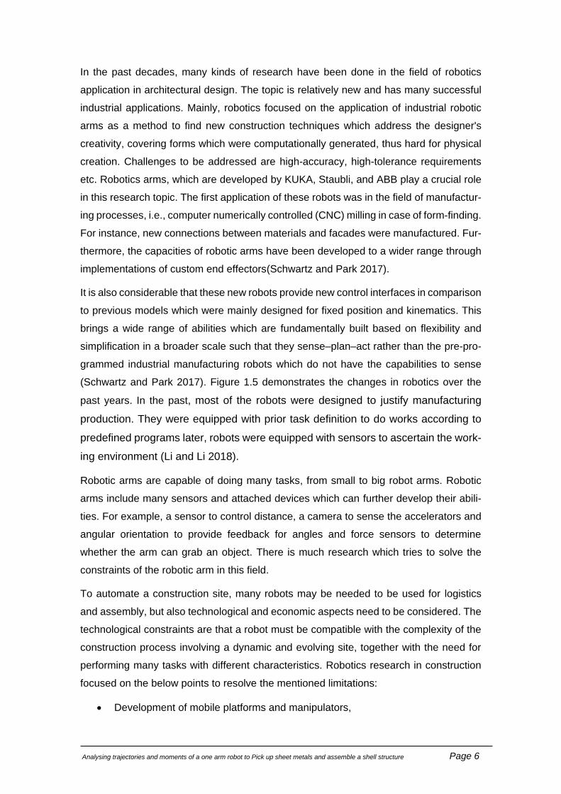
In the past decades, many kinds of research have been done in the field of robotics
application in architectural design. The topic is relatively new and has many successful
industrial applications. Mainly, robotics focused on the application of industrial robotic
arms as a method to find new construction techniques which address the designer's
creativity, covering forms which were computationally generated, thus hard for physical
creation. Challenges to be addressed are high-accuracy, high-tolerance requirements
etc. Robotics arms, which are developed by KUKA, Staubli, and ABB play a crucial role
in this research topic. The first application of these robots was in the field of manufactur-
ing processes, i.e., computer numerically controlled (CNC) milling in case of form-finding.
For instance, new connections between materials and facades were manufactured. Fur-
thermore, the capacities of robotic arms have been developed to a wider range through
implementations of custom end effectors(Schwartz and Park 2017).
It is also considerable that these new robots provide new control interfaces in comparison
to previous models which were mainly designed for fixed position and kinematics. This
brings a wide range of abilities which are fundamentally built based on flexibility and
simplification in a broader scale such that they sense–plan–act rather than the pre-pro-
grammed industrial manufacturing robots which do not have the capabilities to sense
(Schwartz and Park 2017). Figure 1.5 demonstrates the changes in robotics over the
past years. In the past, most of the robots were designed to justify manufacturing
production. They were equipped with prior task definition to do works according to
predefined programs later, robots were equipped with sensors to ascertain the work-
ing environment (Li and Li 2018).
Robotic arms are capable of doing many tasks, from small to big robot arms. Robotic
arms include many sensors and attached devices which can further develop their abili-
ties. For example, a sensor to control distance, a camera to sense the accelerators and
angular orientation to provide feedback for angles and force sensors to determine
whether the arm can grab an object. There is much research which tries to solve the
constraints of the robotic arm in this field.
To automate a construction site, many robots may be needed to be used for logistics
and assembly, but also technological and economic aspects need to be considered. The
technological constraints are that a robot must be compatible with the complexity of the
construction process involving a dynamic and evolving site, together with the need for
performing many tasks with different characteristics. Robotics research in construction
focused on the below points to resolve the mentioned limitations:
• Development of mobile platforms and manipulators,

Analysing trajectories and moments of a one arm robot to Pick up sheet metals and assemble a shell structure Page 7
• Development of control systems and sensory systems integration,
• Re-engineering of processes to suit robotic systems,
• Software development related to supporting the above,
• Use of advanced IT systems to enhance the whole system performance.
Furthermore, for economic concerns which affect the application of a robotic system in
construction, such as:
• Cost vs. benefits
• Changes required for implementing the new system,
• Effect of the new system on the entire organization, which includes health and
safety, and labor unions concerns.
Figure 1.5 Degree of autonomy and complexity from industrial to robots to service robots
In Figure 1.6, different types of on-site robotic construction from large scale robotic
structures, mobile robotic units; or flying robots have been demonstrated. The robotic
construction initiatives in the 1980s and 1990s in Japan were similar to a large scaf-
folding structure, integrating robotic systems to perform different operations. The

Analysing trajectories and moments of a one arm robot to Pick up sheet metals and assemble a shell structure Page 8
WASCOR (WASeda COnstruction Robot) group and the Shimizu Corporation were
among the first initiatives to promote this trend.
Figure 1.6 Large scale robotic mobile robotic units (Sousa et al. 2016)
All in all, the application of robotics is limited to two models, one site and pre-fabrication.
Components of buildings are assembled as per defined rules. The prefabricated building
construction is similar to the assembly of a manufactured product. However, the assem-
bly of components is dependent not only on geometric properties but also on the assem-
bly relationship and spatial restriction information of the components. In Figure 1.7, the
design-to-production approach a shell structure similar to the goal of this research
demonstrates. The Design-to-production models may cause problems and make the pro-
cess complex because manual assembly methods require the use of many manual ma-
chines. Therefore, it causes more loss in resources, including materials, machines, labor,
and computing power. In contrast, combining architectural robotics with the applications
of robotic assembly may lead to improvements. This research is continued to build a
technical and optimal solution considering different aspects (Wu and Kilian 2020).

Analysing trajectories and moments of a one arm robot to Pick up sheet metals and assemble a shell structure Page 9
Figure 1.7 Design to assembly model using manual machines (Wu and Kilian 2020)

Analysing trajectories and moments of a one arm robot to Pick up sheet metals and assemble a shell structure Page 10
Figure 1.8 Robotic for on-site construction (Sullivan 2014)
Problem definition
Until some years ago, the construction industry was far from automation. The construc-
tion industry is one of the less sophisticated sectors of the economy. In recent years, the
construction industry was getting more attention and raised as one of the critical research
areas in the field of robotics. The construction industry is developing new and irregular
shaped structures. With traditional issues in the construction industry, there is required
research aiming to improve the situation. Robotics engineering plays an essential role in
it. Robotics is a solid discipline of study that incorporates the background, knowledge,
and creativity of mechanical, electrical, computer, industrial, and manufacturing engi-
neering.
The main focus of this master thesis is to design and develop the mechanism for a robotic
arm for lifting shell structure elements. The robotic arm kinematic is investigated and
analyzed to accomplish accurately light material lifting and assembling tasks to assist
the construction industry and improve automation. The main intention of designing the
"pick and place machine" is that there will be no need for manual operation for picking
the sheets from the stack and assembling them.
This work focuses on research about the kinematic of one-arm robots by modeling line
diagrams and developing an algorithm for structural analysis of a one-arm robot. The
installation of critical panels of a shell structure is investigated to demonstrate the method
for using the robotic arm on construction sites. The thesis is divided into five chapters; in
the first chapter background of the whole topic is explained. In the second chapter, an
in-depth research is presented to understand better the kinematic of robots and how a
line diagram can be verified for the Grasshopper model. Different applications of robots
are investigated. In the 3rd chapter, the kinematic of the line diagram of the robotic arm
is analyzed, and the result is combined with structural analysis of the robot arm to mini-
mize the moment on the arm.

Analysing trajectories and moments of a one arm robot to Pick up sheet metals and assemble a shell structure Page 11
In the 4th chapter, tracking trajectories of the element assembly are investigated, and the
process of assembling shell structure panels is visualized using Grasshopper. The last
chapter refers to conclusions drawn from this research work and future work that can be
done for improvement of the algorithm and the whole process for further applications.
Analysing trajectories and moments of a one arm robot to Pick up sheet metals and assemble a shell structure Page 12
Fundamentals of Robotics and application of robots in architecture and
construction
Robots for Fabrication of architectural and structural elements
In this part, the application of robots is investigated to evaluate the previous work and
recent research interests. After searching many cases and research projects, it is under-
stood that the best way to compare the case of using robots in civil engineering and
architecture is to divide them into the fabrication of architectural elements and the use of
robots in the construction and assembly processes. One hand is the projects which used
robotic arms for the fabrication of structural elements of the shell structure. On the other
hand, they use the robotic arm to assemble some parts of some structural elements of
different structures, not only shell structures. Accordingly, cases are evaluated to inves-
tigate the workflow of design and computation for geometrical conditions, structural re-
quirements, toolpath development, and fabrication processes using robotic arms.
2.1.1 Robodome: Robotically Fabrication of Complex Curved Geometries
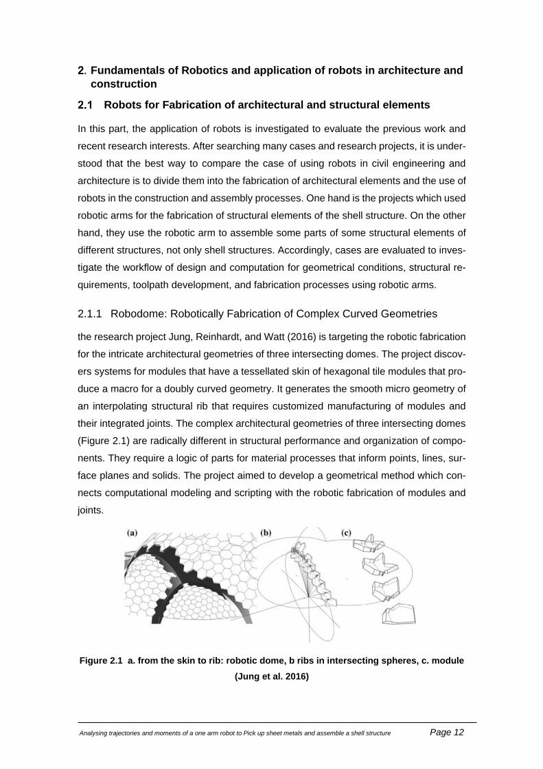
the research project Jung, Reinhardt, and Watt (2016) is targeting the robotic fabrication
for the intricate architectural geometries of three intersecting domes. The project discov-
ers systems for modules that have a tessellated skin of hexagonal tile modules that pro-
duce a macro for a doubly curved geometry. It generates the smooth micro geometry of
an interpolating structural rib that requires customized manufacturing of modules and
their integrated joints. The complex architectural geometries of three intersecting domes
(Figure 2.1) are radically different in structural performance and organization of compo-
nents. They require a logic of parts for material processes that inform points, lines, sur-
face planes and solids. The project aimed to develop a geometrical method which con-
nects computational modeling and scripting with the robotic fabrication of modules and
joints.
Figure 2.1 a. from the skin to rib: robotic dome, b ribs in intersecting spheres, c. module
(Jung et al. 2016)

Analysing trajectories and moments of a one arm robot to Pick up sheet metals and assemble a shell structure Page 13
The other challenge which is discussed in this research is about the application of tes-
sellation into producible segments. The geometry of the model, including an icosahe-
dron, is constructed using three planes in a golden section, where the diagonal length of
the planes equals the diameter of a dome. The vertices of the planes define the points
for the triangles that will hit the sphere with their four corners, thereby creating twelve
equally sized triangles. A recursive projection of the midpoints of each triangle side to-
wards the surface of the sphere creates the next frequency, resulting in the smaller tiling
of the generic hexagon module that constitutes the overall surface when repeated. This
tiling system is excluded from the rib section of the structure, as shown in Figure 2.2. All
the explanations mentioned in these parts are demonstrated in Figure 2.2. For creating
structural ribs, which are the intersecting geometry of two spheres results in an inclined
circle with a center point that anchors the geometry of the rib, which cause an increase
in complexity of geometry, and change in robotic fabrication method from sheet logic to
the subtractive process. Consequently, several different scripts were modeled in McNeil
Rhino and Grasshopper.
Figure 2.2 Geodesic dome: a generic icosahedron, b triangulated tessellation, c. geome-
try for spheres, d. 2 domes intersected, e. rib relative to 2 centers (Jung et al. 2016)
After creating panels and solving the complexity of geometry another challenge raised
with differentiation of the base geometry into the skin and ribs for the practical use of
geometry for robot fabrication which was tested in two methods (Figure 2.3), one method
is regarding the creation of panels based on the desired size and relative to the dimen-
sions and curvature of spheres in the form of a sheet which is efficiently formed by a
milled plaster mold with varying radius (Figure 2.3a–c). Method two is working for the
fabrication of intersecting ribs that follow an intersecting curve between spheres and
connect two tiles arriving from each side. The focus is on the segmentation of the rib into
modules that can be robotically milled from a volume (Figure 2.3d–f).

Analysing trajectories and moments of a one arm robot to Pick up sheet metals and assemble a shell structure Page 14
Figure 2.3 Comparison of the robotic fabrication system (Jung et al. 2016)
The next step of the project is relating to the robotic fabrication of elements which is
including structural ribs and joints using a six-axis robot arm. KUKA|P plugin is used to
adjust the size of the intersecting tiles by rotation in order to make sure that enough
thickness of the material has remained for further processes. The experimental part of
the research is demonstrated in Figure 2.4. (Figure 2.4 a, b) shows the data output of
simulation software and the test for the softness and smoothness of the surface. In (Fig-
ure 2.4, c), the robotic milling followed industry customs for volume milling with support
of added feet that allow steady positioning on the routing bed and precise turnover of the
material sample. Then, modules were robotically milled with a KUKA KR 60-3, using a
standard flat-headed 4KW milling spindle with a 10 mm tool bit and 3 mm stepover, in a
series of robotic protocols that require multiple manual turnovers. A canal is drilled
through each module at the center of the joint to allow for the insertion of a tension cable
(Fig. 6d).
All in all, this project is an excellent example of the process of the design and fabrication
of the complex geometry whit no unique elements. The main challenge is regarding the
manufacturing of panels and penalizing complex curved surfaces. Fabrication of those
complex geometries is the next challenge, while the material is equipped with a high level
of detail. A good understanding of the geometry, material and fabrication tool on the robot
arm conduct to fill the gap between design process and fabrication. Additionally, incor-
porating construction and structural performance which leads to a reconsideration of en-
gineering precedents, and to reformulate this into a novel architectural system. The men-
tioned research is the start point of this thesis. Complex elements of the double-curved

Analysing trajectories and moments of a one arm robot to Pick up sheet metals and assemble a shell structure Page 15
dome are generated and ready for the assembly to construct the dome, which is the main
topic of this thesis.
Figure 2.4 Robotic milling for one rib segment (Jung et al. 2016)

Analysing trajectories and moments of a one arm robot to Pick up sheet metals and assemble a shell structure Page 16
Robotic for assembly of structural elements
2.2.1 Mobile Robotic Brickwork
The research project Dörfler et al. (2016) is a research project which is conducted in ETH
Zurich, Chair of Architecture and Digital Fabrication with the cooperation of Agile & Dex-
terous Robotics Lab. The research starts with evaluating the difference of using robotic
for off- and on-site construction. It is highlighted that the features of construction sites
significantly differ from a factory environment, which makes the fabrication process more
difficult. The environment of building sites is not organized and structured because dur-
ing each phase of construction, shapes of environment change and vary; additionally,
floors maybe not flat, and there are no fixed structures in the surroundings, like the ones
in the manufacturing environment of industrial products. The research considered the
mentioned condition on-site and inspired by the project of the mobile platform dimRob,
which consists of ABB robot arm mounted on a tracked mobile base with a diesel engine.
The dimRob has some limitations, such as lack of sensing and required sensors to allow
the robot to build with high accuracy without being anchored to the ground using fold-out
legs. The improvement of their previous works is the primary motivation of this project.
Figure 2.5 in dimRob the ABB IRB 4600 was selected for the experiment and it was
mounted on a compact mobile track system(Helm et al. 2012)
In the next step of the project, the in-situ fabricator system is designed, which can au-
tonomously complete building tasks directly on a construction site. To decrease the in-
teraction with humans, the robot contains all required sensors which are needed to exe-
cute construction tasks, including sensing, control hardware, and computing systems. In
addition, the necessity for the additional setup of the construction site for the buildings is
avoided by solving the dependency of the robot to external referencing systems. Figure

Analysing trajectories and moments of a one arm robot to Pick up sheet metals and assemble a shell structure Page 17
2.6 demonstrates and explains how this process works; blue pillars and brown floor
shows the geometric description of existing structures within the building space is fit to a
point cloud, captured by the robot when moved to the construction site and notice how
the brown plane, signifying the floor, initially lies above the scan points on the ground but
fits into the points after matching. In the below part of Figure 2.6, a brick wall's geometric
description is adjusted to the real-world sensor measurements of the robot. A mesh re-
laxation algorithm is used to align the individual building blocks' orientation and position
with respect to the true location of the pillar, as well as to level the spacing between the
single bricks.
Figure 2.6 Workspace geometry matching functionality of in situ fabrication (Dörfler et al.
2016)
The next challenge in this project is about the high-level planning of fabrication tasks.
For example, the sequencing of the robot's positions and bricklaying procedures and
computing of the arm and gripper commands. This is implemented using the architectural
planning tool Grasshopper and Rhinoceros. Figure 2.7 shows the communication pro-
cess between design and mobile base and the robot arm movements. Defining coordi-
nates is done in Grasshopper according to the data received from the mobile base and
arm.

Analysing trajectories and moments of a one arm robot to Pick up sheet metals and assemble a shell structure Page 18
The experimental part of the project is a major point of the project. The experiment was
conducted with a dry-stacked double-leaf brick wall which is constructed between two
pillars. For this wall, it is considered that the wall material is separated from the building
structure, and the assembly procedure is designed to solving fundamental problems of
adaptive control strategies, construction sequencing and repositioning operations of in-
situ fabricator (Figure 2.8).
The study shows that it is essential to design a robot for on-site construction independent
to the construction site, while every week, the construction environment faces many
changes. Therefore, to reduce the interaction between the robot, humans and construc-
tion environment, many equipment and methods shall be used for robots on-site to exe-
cute their assigned task with high accuracy.
Figure 2.7 Communication process between different parts (Dörfler et al. 2016)
Figure 2.8 Assembly plan of the brick wall (Dörfler et al. 2016)

Analysing trajectories and moments of a one arm robot to Pick up sheet metals and assemble a shell structure Page 19
2.2.2 Compression arch assembly with robot arm
The Wu and Kilian (2020) research program is based on previous research which is
about the assembly of simple wooden stick elements using robots in order to avoid the
deployment of scaffold. In this study, a compression-only arch is designed using form-
finding principles. It aims to establish a method using a two-arm robotic setup to take
turns to hold up the end of the arch. These studies have demonstrated the possibility of
using robotic assembly as temporary scaffolds for reducing the trouble required to posi-
tion structural members. Using a robot arm for this purpose causes an increase in the
number of required robots which is costly and makes the process more complicated.
Therefore, it is necessary to restrain the quantity of necessary robotic arms. A possible
solution for these limitations is providing axial forces to keep the equilibrium of end of the
arc with the help of an end-effector providing counter axial forces, grasping forces, and
angle adjustments.
Figure 2.9 Different scenario for the number of necessary robotic arms required to main-
tain the structural end (Wu and Kilian 2020)
As shown in Figure 2.9, a five-branch compression-only arch structure generated using
form-finding principles by the "Kangaroo" add-on of Grasshopper. After finding the arc
geometry, each element of the arc which is made from foam is fabricated using hot wire,
a foam was attached to a robotic arm and passed through a hot-wire cutter and for the

Analysing trajectories and moments of a one arm robot to Pick up sheet metals and assemble a shell structure Page 20
element which connected the branches a keystone is designed which is fabricating using
two robotic arms in case that the first robot reaches the maximum reachable radius, the
second robot grabs it and continues the process.
Regarding the assembly process, the results show that the number of required robot
arms increases with the complexity of the structure based on the highest joint valence
(n). Accordingly, the number of robotic arms is n+1. Therefore, two robotic arms can build
a single arch branch.
Figure 2.10 fabrication process of element for the connections of branches (Wu and
Kilian 2020)
Therefore, the assembly sequence plays a key role. An assembly plan is needed to en-
sure that each new block can be maintained in its place by the end effects during robot
repositioning so that they become the new arch ends. In this assembly scenario, new
blocks should be loaded by humans, then the caterpillar tracks find the right angle and
start to move in the right direction and provide enough force to retain the other blocks in
their position. This method has limitations for the assembly of elements with keystone
shape because of the irregular shape. Therefore, some elements on branch intersections
are needed to be assembled manually.
The other challenge is regarding overcome the payload limitation while the robot and the
end effector should provide the axial force to maintain the unfinished arch end. This may
exceed what the caterpillar tracks and could cause problems during the repositioning of
the robotic arms. In Figure 2.11, it is demonstrated that assembling the arc from two
sides leads to a smaller maximum axial force in comparison to starting from one side.

Analysing trajectories and moments of a one arm robot to Pick up sheet metals and assemble a shell structure Page 21
The assembly process is redesigned accordingly to assemble from the supports to the
top to solve that limit.
Figure 2.11 Sequencing planning of robots(Wu and Kilian 2020)
The research project of Wu and Kilian (2020) is an excellent sample of using robots in
construction which starts from designing and form-finding the compression-only arc us-
ing free form methods. It continues with the fabrication of elements using the hot-wire
method. Interaction of robots is one of the critical aspects of this project which opens
many possibilities to design and more efficient assembly plans. It also reduces the waste
of resources (scaffolding). It also gives the ability to the engineer to have a more flexible
design during the construction.

Analysing trajectories and moments of a one arm robot to Pick up sheet metals and assemble a shell structure Page 22
Robot Kinematics
These days, automatic solutions are of interest in achieving most cases, different robot
scenarios. They are very complex and integrate many sensors and effectors, have many
degrees-of-freedoms and require operator interfaces and different programming tools.
The kinematic of robot arms is the one topic which integrates with many complex as-
pects, and it is essential to analyze the kinematics and to plan the trajectory of the robot
from its design to experiment. The kinematic problems, however, are very complex with
complicated computing due to the multi-degree-of-freedom and multilink space mecha-
nisms of the robot. The modern industrial robotic systems, on the other hand, should
implement the task-level control that simplifies the manufacturing task definition for end-
users, because science is more interdisciplinary, and all information should be under-
standable for engineers in different fields (Tatarnikov 2019). The present research inves-
tigates to achieve the mentioned goal by defining the basics in this part. It continues with
the application of them in algorithms in chapter three.
There are two different approaches to control robots. Two very different methods were
recognized; kinematic control and dynamic control. There is also a method which inte-
grates both approaches. These two approaches achieve robot control based on mathe-
matical calculation. This research focuses on the kinematic approach is focused
(Schwartz and Park 2017).
Figure 2.12 Relationship between forward and inverse kinematics(El-Sherbiny,
Elhosseini, and Haikal 2018)
In the kinematic method, the robot is programmed by finding the joint angles. There are
two methods for finding the joint angles which are forward kinematics and inverse kine-
matics. In forward kinematics, a set of joint angles is used to determine the final position
and orientation of the end effector. On the other hand, the inverse kinematic method
determines the joint angles from a given position and orientation of the end effector (Fig-
ure 2.12).

Analysing trajectories and moments of a one arm robot to Pick up sheet metals and assemble a shell structure Page 23
This research investigates, how a robot visualization of a six degree of freedom robot
arm (KUKA titan 1000 L750) by Grasshopper can be useful for engineers working in the
field of robotics. Additionally, it shows, how it can be used effectively to improve the
capacity of the robot arm in construction works.
Figure 2.13 KUKA titan 1000 L750 (KUKA Roboter GmbH 2016)
2.3.1 Forward kinematic: Denavit Hartenberg method
In this case, the robot is assumed as a rigid robot. Forward kinematics provides a method
to find the relation between the robot's joints variables and the position and orientation
of the end effector. Joints variables include the angles between links and rotation or
revolution (Mark W. Spong, Seth Hutchinson 2008).
Robotic arms consist of links and joints. In this research, all joints assumed as single-
degree-of-freedom. Therefore, the action of each joint can be defined by a single real
number, and in this case, the type of joints is revolute joint, and the angle of rotation is
defined by a number. The primary purpose of forward kinematic is to calculate the effect
of the entire set of joint variables.
The Denavit-Hartenberg notation is a method which assigns reference coordinates to
each degree of freedom. In this system, Ai is a homogenous transformation which con-
sists of four basic transformations. Below, the transformation matrix is shown that trans-
forms from frame Ki-1 to frame Ki within a robot kinematic link chain. The below calculation
is done with the help of (Tatarnikov 2019).

Analysing trajectories and moments of a one arm robot to Pick up sheet metals and assemble a shell structure Page 24
𝑻𝒊𝒊−𝟏 = 𝑹𝒐𝒕(𝒛, 𝜽𝒊)𝑻𝒓𝒂𝒏𝒔(𝟎, 𝟎, 𝒅𝒊)𝑻𝒓𝒂𝒏𝒔(𝒂𝒊, 𝟎, 𝟎)𝑹𝒐𝒕(𝒙, 𝜶𝒊) =
[
𝐜𝐨𝐬 𝜽𝒊 − 𝐬𝐢𝐧 𝜽𝒊 𝐜𝐨𝐬 𝜶𝒊 𝐬𝐢𝐧 𝜽𝒊 𝐬𝐢𝐧 𝜶𝒊 𝒂𝒊 𝐜𝐨𝐬 𝜽𝒊
𝐬𝐢𝐧 𝜽𝒊 𝐜𝐨𝐬 𝜽𝒊 𝐜𝐨𝐬 𝜶𝒊 − 𝐜𝐨𝐬 𝜽𝒊 𝐬𝐢𝐧 𝜶𝒊 𝒂𝒊 𝐬𝐢𝐧 𝜽𝒊
𝟎 𝐬𝐢𝐧 𝜶𝒊 𝐜𝐨𝐬 𝜶𝒊 𝒅𝒊
𝟎 𝟎 𝟎 𝟏
] [Eq. 2.1]
Accordingly, in case of a robot with N degree of freedom, the total transformation be-
tween the first frames K0, the base of the first kinematic link, and the last KN, the end-
effector, is the output of multiplication of matrix of all the D-H transformation matrices:
𝑻𝑵𝟎 = 𝑻𝟏
𝟎 𝑻𝟐𝟏 ⋯ 𝑻𝑵
𝑵−𝟏 = [
𝒍𝒙 𝒎𝒙 𝒏𝒙 𝒑𝒙
𝒍𝒚 𝒎𝒚 𝒏𝒚 𝒑𝒚
𝒍𝒛 𝒎𝒛 𝒏𝒛 𝒑𝒛
𝟎 𝟎 𝟎 𝟏
] = [ 𝒍 �⃗⃗⃗⃗� �⃗⃗⃗� �⃗⃗⃗�𝟎 𝟎 𝟎 𝟏
] = [𝑹 �⃗⃗⃗�
�⃗⃗⃗�𝑻 𝟏] [Eq. 2.2]
Where R - corresponds to a 3x3 matrix, representing rotation; �⃗⃗⃗� - corresponds to a 3x1
matrix (vector) that represents a translation.
Then, the robot transforms for 6 degrees of freedom robot as KUKA 1000 titan is:
𝑻𝟔𝟎 = 𝑻𝟏
𝟎 𝑻𝟐𝟏 𝑻 𝑻𝟒
𝟑 𝑻𝟓𝟒 𝑻 = [
𝒍𝒙 𝒎𝒙 𝒏𝒙 𝒑𝒙
𝒍𝒚 𝒎𝒚 𝒏𝒚 𝒑𝒚
𝒍𝒛 𝒎𝒛 𝒏𝒛 𝒑𝒛
𝟎 𝟎 𝟎 𝟏
]𝟔𝟓
𝟑𝟐 [Eq. 2.3]
This overall transformation describes the position of a robot tool flange in Cartesian rel-
ative coordinates to a world coordinate frame, which generally is located at the robot root
(base). If the robot has a tool or different base, world coordinate does not match the robot
root, and it will require multiplying the transformation matrix 𝑇60 to the tool matrix or base
matrix.
Transformation matrices for the robot are the following:
𝑻 = [
𝐜𝐨𝐬 𝜽𝟏 𝟎 −𝐬𝐢𝐧 𝜽𝟏 𝒂𝟏 𝐜𝐨𝐬 𝜽𝟏
𝐬𝐢𝐧 𝜽𝟏 𝟎 𝐜𝐨𝐬 𝜽𝒊 𝒂𝟏 𝐬𝐢𝐧 𝜽𝟏
𝟎 −𝟏 𝟎 𝒅𝟏
𝟎 𝟎 𝟎 𝟏
]𝟏𝟎 [Eq. 2.4]
𝑻 = [
𝐜𝐨𝐬 𝜽𝟐 − 𝐬𝐢𝐧 𝜽𝟐 𝟎 𝒂𝟐 𝐜𝐨𝐬 𝜽𝟐
𝐬𝐢𝐧 𝜽𝟐 𝐜𝐨𝐬 𝜽𝟐 𝟎 𝒂𝟐 𝐬𝐢𝐧 𝜽𝟐
𝟎 𝟎 𝟏 𝟎𝟎 𝟎 𝟎 𝟏
]𝟐𝟏 [Eq. 2.5]
𝑻 = [
𝐜𝐨𝐬 𝜽𝟑 𝟎 − 𝐬𝐢𝐧 𝜽𝟑 𝒂𝟑 𝐜𝐨𝐬 𝜽𝟑
𝐬𝐢𝐧 𝜽𝟑 𝟎 𝐜𝐨𝐬 𝜽𝟑 𝒂𝟑 𝐬𝐢𝐧 𝜽𝟑
𝟎 −𝟏 𝟎 𝟎𝟎 𝟎 𝟎 𝟏
]𝟑𝟐 [Eq. 2.6]

Analysing trajectories and moments of a one arm robot to Pick up sheet metals and assemble a shell structure Page 25
𝑻 = [
𝐜𝐨𝐬 𝜽𝟒 𝟎 𝐬𝐢𝐧 𝜽𝟒 𝟎𝐬𝐢𝐧 𝜽𝟒 𝟎 − 𝐜𝐨𝐬 𝜽𝒊 𝟎
𝟎 𝟏 𝟎 𝒅𝟒
𝟎 𝟎 𝟎 𝟏
]𝟒𝟑 [Eq. 2.7]
𝑻 = [
𝐜𝐨𝐬 𝜽𝟓 𝟎 − 𝐬𝐢𝐧 𝜽𝟓 𝟎𝐬𝐢𝐧 𝜽𝟓 𝟎 𝐜𝐨𝐬 𝜽𝟓 𝟎
𝟎 −𝟏 𝟎 𝟎𝟎 𝟎 𝟎 𝟏
]𝟓𝟒 [Eq. 2.8]
𝑻 = [
𝐜𝐨𝐬 𝜽𝟔 − 𝐬𝐢𝐧 𝜽𝟔 𝟎 𝟎𝐬𝐢𝐧 𝜽𝟔 𝐜𝐨𝐬 𝜽𝟔 𝟎 𝟎
𝟎 𝟎 𝟏 𝒅𝟔
𝟎 𝟎 𝟎 𝟏
]𝟔𝟓 [Eq. 2.9]
Therefore, after the formation of each matrix and multiplication of them. The overall trans-
formation matrix is calculated, and the results are as below:
𝒍𝒙 = 𝐬𝟏(𝐬𝟒𝐜𝟓𝐜𝟔 + 𝐜𝟒𝐬𝟔) + 𝐜𝟏(−𝐬𝟐𝟑𝐬𝟓𝐜𝟔 + 𝐜𝟐𝟑(𝐜𝟒𝐜𝟓𝐜𝟔 − 𝐬𝟒𝐬𝟔)) [Eq. 2.10]
𝒍𝒚 = −𝐜𝟏(𝐬𝟒𝐜𝟓𝐜𝟔 + 𝐜𝟒𝐬𝟔) + 𝐬𝟏(−𝐬𝟐𝟑𝐬𝟓𝐜𝟔 + 𝐜𝟐𝟑(𝐜𝟒𝐜𝟓𝐜𝟔 − 𝐬𝟒𝐬𝟔)) [Eq. 2.11]
𝒍𝒛 = −𝐜𝟔(𝐬𝟐𝟑𝐜𝟒𝐜𝟓 + 𝐜𝟐𝟑𝐬𝟓) + 𝐬𝟐𝟑𝐬𝟓𝐬𝟔 [Eq. 2.12]
𝒎𝒙 = 𝐜𝟔(𝐬𝟏𝐜𝟒 − 𝐜𝟏𝐜𝟐𝟑𝐬𝟒) − 𝐬𝟔(𝐬𝟏𝐬𝟒𝐜𝟓 + 𝐜𝟏(𝐜𝟐𝟑𝐜𝟒𝐜𝟓 − 𝐬𝟐𝟑𝐬𝟓)) [Eq. 2.13]
𝒎𝒚 = 𝐜𝟏(−𝐜𝟒𝐜𝟔 + 𝐜𝟓𝐬𝟒𝐬𝟔) − 𝐬𝟏(−𝐬𝟐𝟑𝐬𝟓𝐬𝟔 + 𝐜𝟐𝟑(𝐬𝟒𝐜𝟔 + 𝐜𝟒𝐜𝟓𝐬𝟔)) [Eq. 2.14]
𝒎𝒛 = 𝐬𝟐𝟑𝐬𝟒𝐜𝟔 + 𝐬𝟔(𝐬𝟐𝟑𝐜𝟒𝐜𝟓 + 𝐜𝟐𝟑𝐬𝟓) [Eq. 2.15]
𝒏𝒙 = −𝐬𝟏𝐬𝟒𝐬𝟓 − 𝐜𝟏(𝐬𝟐𝟑𝐜𝟓 + 𝐜𝟐𝟑𝐜𝟒𝐬𝟓) [Eq. 2.16]
𝒏𝒚 = −𝐬𝟏𝐬𝟐𝟑𝐜𝟓 + 𝐬𝟓(−𝐬𝟏𝐜𝟐𝟑𝐜𝟒 + 𝐜𝟏𝐬𝟒) [Eq. 2.17]
𝒏𝒛 = −𝐜𝟐𝟑𝐜𝟓 + 𝐜𝟒𝐬𝟐𝟑𝐬𝟓 [Eq. 2.18]
𝒑𝒙 = −𝐝𝟔𝐬𝟏𝐬𝟒𝐬𝟓 + 𝐜𝟏(𝐚𝟏 + 𝐚𝟐𝐜𝟐 − 𝐬𝟐𝟑(𝐝𝟒 + 𝐝𝟔𝐜𝟓) + 𝐜𝟐𝟑(𝐚𝟑 − 𝐝𝟔𝐜𝟒𝐬𝟓)) [Eq. 2.19]
𝒑𝒚 = 𝐝𝟔𝐜𝟏𝐬𝟒𝐬𝟓 + 𝐬𝟏(𝐚𝟏 + 𝐚𝟐𝐜𝟐 − 𝐬𝟐𝟑(𝐝𝟒 + 𝐝𝟔𝐜𝟓) + 𝐜𝟐𝟑(𝐚𝟑 − 𝐝𝟔𝐜𝟒𝐬𝟓)) [Eq. 2.20]
𝒑𝒛 = 𝐝𝟏 − 𝐜𝟐𝟑(𝐝𝟒 + 𝐝𝟔𝐜𝟓) − 𝐚𝟐𝐬𝟐 + 𝐬𝟐𝟑(−𝐚𝟑 + 𝐝𝟔𝐜𝟒𝐬𝟓) [Eq. 2.21]
Where 𝒔𝒊 = 𝐬𝐢𝐧 𝜽𝒊, 𝒄𝒊 = 𝐜𝐨𝐬 𝜽𝒊, 𝒔𝟐𝟑 = 𝐬𝐢𝐧(𝜽𝟐 + 𝜽𝟑), 𝒄𝟐𝟑 = 𝐜𝐨𝐬(𝜽𝟐 + 𝜽𝟑) [Eq. 2.22]
Now it is necessary to find the values of parameters of the Denavit-Hartenberg notation.
According to Denavit-Hartenberg notation, any robot manipulator can be described kin-
ematically by giving the values of four quantities for each link of robot joint:
Twist angle – α,

Analysing trajectories and moments of a one arm robot to Pick up sheet metals and assemble a shell structure Page 26
Joint angle – θ,
Link length – a,
Joint offset – d.
Table 2.1 Denavit-Hartenberg parameters (Mark W. Spong, Seth Hutchinson 2008)
A robot arm with n joints will have n + 1 links because each joint connects two links. Two
of the mentioned parameters describe the link itself, and two describe the link's connec-
tion to a neighboring link. Figure 2.14 and Figure 2.15 represent Denavit-Hartenberg
parameters and positive values.
Figure 2.14 Visualization of DH parameters (Mark W. Spong, Seth Hutchinson 2008)
Figure 2.15 Positive values for DH parameters (Mark W. Spong, Seth Hutchinson 2008)

Analysing trajectories and moments of a one arm robot to Pick up sheet metals and assemble a shell structure Page 27
Figure 2.16 Robot dimension (KUKA Roboter GmbH 2016)
D-H parameters for KUKA titan 1000 are measured after assigning the frames according
to basics which were shown before. The measured values are shown in Table 2.2. All
the ai and di values can be found in the robot datasheet.
Table 2.2 Calculated DH parameters
Link θi(degree) αi(degree) ai(m) di (m)
1 0 90 0.6 1.1
2 90 0 or 180 1.4 0
3 0 90 or -90 0.065 0
4 0 -90 0 1.6
5 0 90 or -90 0 0
6 0 0 0 0.372
According to the found values and related calculation, the frame coordinate of the end
effector of the robot (standing in the shown position in Figure 2.17) can be found by
below Homogenous Transformation Matrix
𝑇60 = 𝑇1
0 𝑇21 ⋯ 𝑇6
5 = [
0 0 1 0.9150 −1 0 01 0 0 1.120 0 0 1
]

Analysing trajectories and moments of a one arm robot to Pick up sheet metals and assemble a shell structure Page 28
The result of this part of the research is used in chapter three, and the results are used
to develop the algorithm which simplifies all the calculation and have an online visuali-
zation of the kinematic to prevent long calculations and time.
Figure 2.17 Assumed the position of the robot for calculation(Gupta, Chittawadigi, and
Saha 2017)

Analysing trajectories and moments of a one arm robot to Pick up sheet metals and assemble a shell structure Page 29
2.3.2 Inverse kinematic
One other method which is used mostly for path planning and trajectory definition of
robotic arms is the inverse kinematic method. The inverse kinematic problem of manip-
ulators is an essential issue, needed for controlling the end effector. The inverse kine-
matic solution is time intensive with respect to computations. An end effector performs
its task in the cartesian space, but actuators work in joint space. Cartesian space in-
cludes an orientation matrix and position vector. However, joint space is represented by
joint angles. The conversion of the position and orientation of a manipulator end-effector
from Cartesian space to joint space is called an inverse kinematics problem. There are
two solution approaches, namely, geometric and algebraic, used for deriving the inverse
kinematics solution analytically (Kucuk and Bingul 2007).
Figure 2.18 Solution of inverse kinematic(Kucuk and Bingul 2007).
To find the geometric solution, we divide the spatial geometry of the manipulators into
several plane geometry. It applies to simple structures like 2-DOF planar manipulator
whose joints are both revolute, and link lengths are l1 and l2 (see Figure 2.18). In order
to derive the kinematic equations for the planar manipulator. The components of the
point P (px and py) are determined as follows (Kucuk and Bingul 2007).
To find the function of teta and find the relation between values in the below figure, we
need to solve inverse kinematic. Although the end effector in 2D has simple kinematics,
its inverse kinematics solution (based on a geometric approach) is very cumbersome.
The algebraic solution is similar to what was explained for forward kinematic.
Inverse kinematics change the motion plan to axes actuator trajectories for the robot.
Figure 2.19 shows the simple example of inverse kinematics using a robotic arm which
has upper and lowers arm and angles. It is determined to reach the target point.
All in all, mathematical based calculation of inverse kinematic for the robots for a high
degree of freedom is time-consuming and the calculation is costly. Therefore, in this re-
search, a model is developed in Grasshopper based on the geometrical solution for the
6 degrees of freedom robot.

Analysing trajectories and moments of a one arm robot to Pick up sheet metals and assemble a shell structure Page 30
The next chapter goes through the technical and simulation aspects of the recent re-
search by modeling and discussing the solution using Grasshopper and Rhino.
Figure 2.19 Simple example of inverse kinematic

Analysing trajectories and moments of a one arm robot to Pick up sheet metals and assemble a shell structure Page 31
Analysis of robotic arm
In all applications of robotic arms, it is necessary to model and simulate the robot in
different ways, including motion analysis, control analysis, mechanical analysis and dy-
namic analysis. For example, mechanical engineers concern about the performance of
the robot body and the efficiency of the robot. For this, they are mostly using Solid work
and Ansys for design and analysis of the robot body. In addition, each robot shall be
analyzed for each specific task according to the environmental situation. Especially, mo-
tion analysis of the end effector based on environmental constraints leads to inputs for
the control system, which provides the commands for joint actuators of the manipulator.
Therefore, the control needs an accurate analysis of the characteristics of the mechani-
cal structure, actuators, and sensors. The main purpose of all these analyses is to intro-
duce and calculate mathematical models to find motion control strategies of robot ele-
ments.
By using MATLAB, a lot of research is done to verify the theory and at the same time to
develop a tool for simplifying the analysis that simulates the movements of the robotic
arm. In addition, in MATLAB, it is possible to use co-simulators with other software to
have a complete mechanical system. This is done, for example, in Aktas, Pehlivan, and
Esen (2017), In this case, MATLAB and ADAMS are used to improve design efficiency,
shorten the design process, reduce costs and allow the system to operate at optimum
conditions. Figure 3.1 shows the workflow of the co-simulation process.
Figure 3.1 Diagram of the co-simulation system(Aktas et al. 2017)

Analysing trajectories and moments of a one arm robot to Pick up sheet metals and assemble a shell structure Page 32
The mentioned method of simulation and analysis of robotic arms is integrated with many
codes and complex mathematical formulas. This is out of interest for engineers who want
to use robots as a tool to make their job easier. Therefore, a combination of Rhino and
Grasshopper can bring a friendlier user interface and a more interactive environment.
This can be archived by integrating the geometry of robots and running the analysis
within one software. The robot arm's kinematic model is useful for determining the cor-
relation between forces and torques applied to the joints as well as the forces and mo-
ments applied to the end effector in static equilibrium (Sciavicco and Siciliano 2000).
In order to model a robot arm kinematic in Grasshopper, there are many plugins and
component which can be installed on the Grasshopper core additionally. RoboDK, HAL
Robotics, KUKA PRC are examples of famous plugins in Grasshopper which mostly fo-
cus on path planning for milling, 3D printing and winding. There are many robot models
from many manufacturers like KUKA and ABB robots, as well as many different tools
which simplify the modeling and simulation and can be counted as an advantage of these
plugins. Another positive point is that the mentioned plugins are also efficient for collision
checking and detecting axes clashes during the process. On the other hand, these
plugins have limitations in modeling the payloads and the effect of payload and effector
on the robot.
Figure 3.2 Plugins for robot modeling in Grasshopper
For example, it is not possible to check the stability of a robot under a certain load on the
end effector. The stability of a robotic arm depends on many parameters. These need to
be analyzed and investigated during the design and manufacturing process of the robot
arms. Examples for such parameters, including dynamic parameters, are the motor
power, stabilizers, material strength and the weight of the robot. By considering all pa-
rameters, manufactures can analyze the robot and provide diagrams in the datasheet of
their products, as shown in Figure 3.3. These help the users to check if the robot is able
to handle a specific task. As you can see, the diagram shows that the payload capacity
is based on the distance between the center of gravity of the payload and the end flange
of the robot. The capacity of the robot decreases when the mentioned distance in-
creases.

Analysing trajectories and moments of a one arm robot to Pick up sheet metals and assemble a shell structure Page 33
Figure 3.3 Payload diagram for KR 1000 titan(KUKA Roboter GmbH 2016)
The purpose of this research is to handle and assemble panels to construct a shell struc-
ture. Therefore, grippers play a crucial role. Grippers are systems which provide tempo-
rary contact with the object to be handled. The main task of grippers is to ensure the
positioning and orientation of the payload when moving and carrying. The main concern
is about the produced forces. The holding force can act on a point, line or surface
(Monkman et al. 2006).
The pick and place processes are acting as a loop, as shown in Figure 3.4demonstrates
the flowchart of these maneuvers. There are many different types of grippers which can
be used in different applications. The choice of a gripper depends mainly on the work it
has to perform. According to Monkman et al. (2007), each gripper should be analyzed
from a different aspect, as explained in Figure 3.5.
Figure 3.4 Gripper working loop

Analysing trajectories and moments of a one arm robot to Pick up sheet metals and assemble a shell structure Page 34
Taking into account the impact of the gripper and the payload on the stability of the robot
arm, a method is developed to reduce the moment in the robot base from the weight of
the payload in a static configuration. The idea of the method for reducing the momentum
comes from Figure 3.6. In the next part, an algorithm is developed to calculate the ap-
plied moment caused by the payload and then to select the pick point in a way to reduce
the leverage arm. This will lead to a lower moment and increase the working radius of
the robot arm according to the payload diagram.
Figure 3.5 Requirements for selecting gripper (Monkman et al. 2007)
Figure 3.6 Methodology of calculating the moment of the robot element
Requierments for selecting gripper
Technological
prehension time
gripping path
grabbing force
Effects from the object
mass
design
dimenssions
Factors related to environmental
parameters
axial accelerations
positional accuracy
connection specifications
Factors related to handling
equipment
feeding conditions
vibration
storage conditions

Analysing trajectories and moments of a one arm robot to Pick up sheet metals and assemble a shell structure Page 35
The algorithm process, shown in Figure 3.7, is implemented. It determines the weight of
each panel and assigns it to calculate the moments in the base of the robot.
Figure 3.7 Workflow for assign weight to panels and minimize the moment at joints
Based on the explanations of the restrictions of current plugins, the line diagram of the
robot arm is modeled in order to simulate and analyses the kinematic of the robot and to
evaluate how it is possible to investigate the possible solution for the restrictions of the
plugins. Therefore, an algorithm is developed in this chapter which imitates a one-arm
robot as a line diagram and minimizes the moment by selecting the best grabbing point
according to the panel's weight. Modeling and analyzing the robot kinematic in Grass-
hopper has many benefits. The parametric control of the robot kinematics avoids many
mathematical calculations for every state of the robot. In addition, Grasshopper and
Rhino provide an excellent opportunity to visualize theoretical meanings. The research
continued in the next chapter. An algorithm is developed by using the KUKA PRC plugin
to simulate the installation of a critical section of shell structure, to track the trajectories
and to break down the trajectory motions of one arm.
For modeling, the line diagram of the following process is applied to each degree of
freedom to model the robot according to Forward and Inverse kinematic formulation.
Figure 3.8 shows the overview of the algorithm for modeling the Forward kinematic.
Figure 3.8 Overview of modeling of forward kinematic
Calculate Volume of
Panels
Calcualte weight of
panels acc. to density
Find the Center of Gravity
Calculate distance to joint
center
Calculate Momenet
Find the best pick up point

Analysing trajectories and moments of a one arm robot to Pick up sheet metals and assemble a shell structure Page 36
Figure 3.9 shows an overview of the algorithm for modeling the Inverse kinematic.
Figure 3.9 Overview of modeling of Inverse kinematic
The research continued in the next part with the explanation of the line diagram element
and the detailed explanation of the development of algorithms in Grasshopper.

Analysing trajectories and moments of a one arm robot to Pick up sheet metals and assemble a shell structure Page 37
Line diagram for kinematic analysis of robotic arm
The solid model of the robotic arm was created within Rhino. Based on case studies and
evaluations of various projects with robots, KUKA robot KR 1000 L750 titan (Figure 3.10)
with 6 degrees of freedom was chosen. This is due to its long reach arm, the wide work-
ing area with a maximum reach of 3601 mm and the maximum payload of 750 kg, which
gives engineers many advantages for the use of robots on the construction site.
Figure 3.10 KUKA Titan 1000 (KUKA Roboter GmbH 2016)
According to the manufacturer’s datasheet, the required joint and arm' length data are
exported from the datasheet. An excerpt from this data sheet is given in Figure 3.11.
Figure 3.11 Working envelope, KR 1000 L750 titan (KUKA Roboter GmbH 2016)
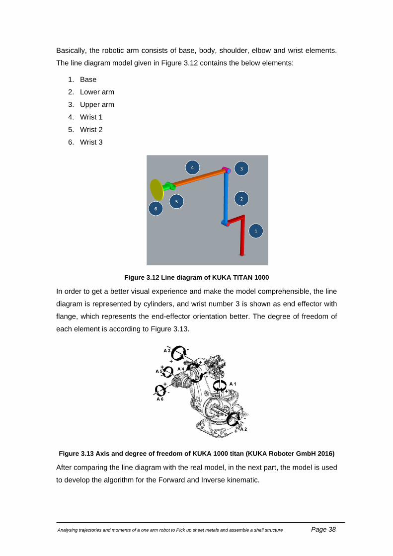
Analysing trajectories and moments of a one arm robot to Pick up sheet metals and assemble a shell structure Page 38
Basically, the robotic arm consists of base, body, shoulder, elbow and wrist elements.
The line diagram model given in Figure 3.12 contains the below elements:
1. Base
2. Lower arm
3. Upper arm
4. Wrist 1
5. Wrist 2
6. Wrist 3
Figure 3.12 Line diagram of KUKA TITAN 1000
In order to get a better visual experience and make the model comprehensible, the line
diagram is represented by cylinders, and wrist number 3 is shown as end effector with
flange, which represents the end-effector orientation better. The degree of freedom of
each element is according to Figure 3.13.
Figure 3.13 Axis and degree of freedom of KUKA 1000 titan (KUKA Roboter GmbH 2016)
After comparing the line diagram with the real model, in the next part, the model is used
to develop the algorithm for the Forward and Inverse kinematic.

Analysing trajectories and moments of a one arm robot to Pick up sheet metals and assemble a shell structure Page 39
3.1.1 Forward kinematic of robot arm line diagram
According to the previous section, the line diagram of the robot is now prepared for the
implementation of the forward kinematic based on the theory of Denavit Hartenberg
(DH).
According to the investigations in the previous chapter, the DH method is used to assign
the coordinate frame for each joint according to the method for measuring the DH pa-
rameters discussed and calculated in chapter 2.
Figure 3.14 demonstrates an overview of the algorithm.
Figure 3.14 Overview of the Forward kinematic algorithm
The process is explained step by step below.
Step 0: Finding the joint center and plane
At first, it is necessary to find the joint center for each axis and define a plane
according to its degree of freedom. There are six axes in this robot. Joint centers
and planes are determined accordingly (Figure 3.13). A detailed description re-
garding the type of inputs and the outputs obtained from each component is men-
tioned in the following steps.

Analysing trajectories and moments of a one arm robot to Pick up sheet metals and assemble a shell structure Page 40
Figure 3.15 Defining joint's planes
Table 3.1 Input for Plane component in Figure 3.15
Required Input Given input Description
Origin Point The point on the center of each joint
Table 3.2 Output from Plane component in Figure 3.15
Type of output Output Description
Plane XYZ local frame Coordinate plane for each joint
The following output can be visualized in Rhino:
Table 3.3 Joints coordinate plane
Step 1: Model axis 1
First, the location of the base of the robot shall be determined using a single point
to create a XY plane by the “XY Plane” command which produces a plane in the
given point, as shown in Figure 3.16. Then the degree of freedom is defined by
the “Rotate Plane” command and the “Geometry” of the element related to axis

Analysing trajectories and moments of a one arm robot to Pick up sheet metals and assemble a shell structure Page 41
one is oriented by the “Orient” command in the desired direction, as explained in
Table 3.4 and Table 3.5.
Figure 3.16 Modelling of axis1
Table 3.4 Input for “Rotate Plane” component in Figure 3.16 perform plane rotation
around z-axis
Required Input Given input Description
Plane Plane at the base location Plane to rotate
Angle Number slider as joint
value
Rotation around plane z-axis in ra-
dians
Table 3.5 Output of Rotate Plane component
Type of output Output Description
Plane Axis 1 rotated plane Rotated plane
The following output can be visualized in Rhino:
Figure 3.17 Rotated position of axis 1
Base point
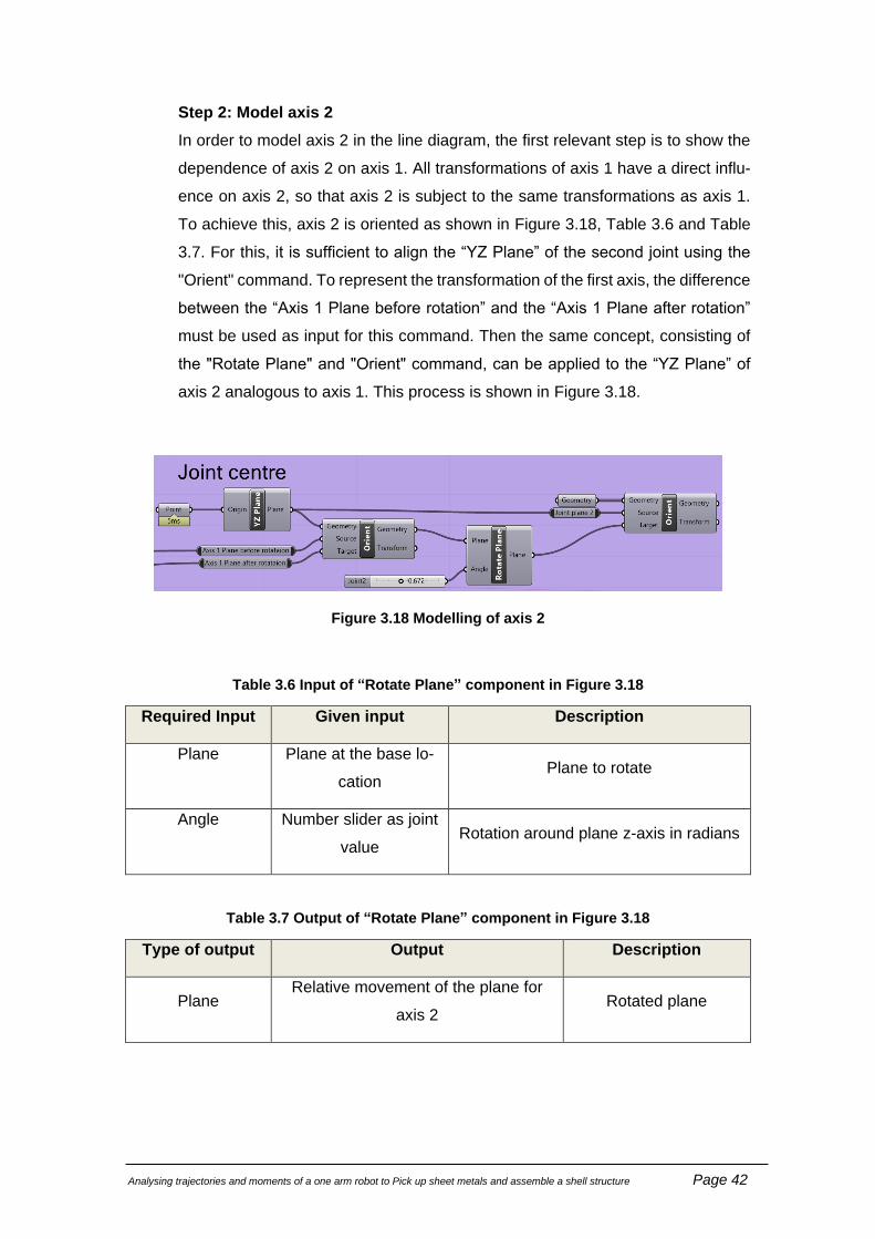
Analysing trajectories and moments of a one arm robot to Pick up sheet metals and assemble a shell structure Page 42
Step 2: Model axis 2
In order to model axis 2 in the line diagram, the first relevant step is to show the
dependence of axis 2 on axis 1. All transformations of axis 1 have a direct influ-
ence on axis 2, so that axis 2 is subject to the same transformations as axis 1.
To achieve this, axis 2 is oriented as shown in Figure 3.18, Table 3.6 and Table
3.7. For this, it is sufficient to align the “YZ Plane” of the second joint using the
"Orient" command. To represent the transformation of the first axis, the difference
between the “Axis 1 Plane before rotation” and the “Axis 1 Plane after rotation”
must be used as input for this command. Then the same concept, consisting of
the "Rotate Plane" and "Orient" command, can be applied to the “YZ Plane” of
axis 2 analogous to axis 1. This process is shown in Figure 3.18.
Figure 3.18 Modelling of axis 2
Table 3.6 Input of “Rotate Plane” component in Figure 3.18
Required Input Given input Description
Plane Plane at the base lo-
cation Plane to rotate
Angle Number slider as joint
value Rotation around plane z-axis in radians
Table 3.7 Output of “Rotate Plane” component in Figure 3.18
Type of output Output Description
Plane Relative movement of the plane for
axis 2 Rotated plane

Analysing trajectories and moments of a one arm robot to Pick up sheet metals and assemble a shell structure Page 43
Table 3.8 Input of “Orient component” in Figure 3.18
Required Input Given input Description
Geometry YZ plane related to axis two at the joint
point Geometry
Source Axis 1 Plane before rotation Plane
Target Axis 1 Plane after rotation Plane
Table 3.9 Output of “Orient component” in Figure 3.18
Type of output Output Description
Geometry Reoriented geometry Transformation data
The following output can be visualized in Rhino:
Figure 3.19 Rotated position of axis 2
Step 3 to 6: Model axis 3 to 6
For modeling axis 3 to 6, the same procedure as step 2 is applied for all other
axes. The first relative frame is defined as described in the previous section to
get to the position of axis 3 to 6 influenced by the transformation of the previous
related axes. Then, it is oriented once, as explained in Figure 3.20, Table 3.6 and
Table 3.7. Then to define the degree of freedom and choosing the rotation of axis
3 to 6, “Rotate Plane” and “Orient” component are used analogously to step 1.
The following outputs can be visualized in Rhino:

Analysing trajectories and moments of a one arm robot to Pick up sheet metals and assemble a shell structure Page 44
Algorithm related to axis 3 Oriented element of axis 3
Algorithm related to axis 4 Oriented element of axis 4
Algorithm related to axis 5 Oriented element of axis 5
Algorithm related to axis 6 Oriented element of axis 6
Figure 3.20 Summary of modeling axis 3 to 6

Analysing trajectories and moments of a one arm robot to Pick up sheet metals and assemble a shell structure Page 45
The output of all these steps are the lists in Figure 3.21, which shows the position and
orientation of the end effector for given joint angles.
Figure 3.21 Result of forward kinematic analysis of the line diagram

Analysing trajectories and moments of a one arm robot to Pick up sheet metals and assemble a shell structure Page 46
3.1.2 Modeling of line diagram based on Inverse kinematic
This part examines an alternative to forward kinematics. The Visualization of robot kine-
matics in Rhino and Grasshopper enables engineers to understand robot kinematics to
use in multidisciplinary projects.
Figure 3.22 shows the overview of the algorithm, and a different part of the algorithm is
named on the picture.
Figure 3.22 Overview of the inverse kinematic algorithm
Step 1: In the first step, modeling starts with assigning the joint center of the
base, wrist one wrist 2 to point A, B and C (Figure 3.23).
Figure 3.23 Import joint center to Grasshopper
Step 2: Defining the location of the robot by using a single point as the origin of
the “XY Plane” to demonstrate the location of the robot’s base (Figure 3.24). The
visualization of this step is shown in Figure 3.25.

Analysing trajectories and moments of a one arm robot to Pick up sheet metals and assemble a shell structure Page 47
Figure 3.24 Defining base plane position
Figure 3.25 Visualization the output of step 2
Step 3: Based on the theory of inverse kinematics, the input of the algorithm is
the target position of the end effector. Therefore, the final position of the end
effector is defined by a plane which consists of 3 points, as you can see in Figure
3.26. The plane is located on a surface of the cube to have a better demonstration
of the purpose of the study, as shown in Figure 3.27.
Figure 3.26 Defining target plane
Figure 3.27 Visualization the output of step 3

Analysing trajectories and moments of a one arm robot to Pick up sheet metals and assemble a shell structure Page 48
Step 4: Find the rotation angle of axis 1
As shown in Figure 3.28, a vector from the base point to the origin of the target
point is demonstrated. The rotation of axis 1 is calculated by comparing the x-
axis of the base plane with the given vector to get the direction of the target plane.
There are two positions for the related element to axis 1 to reach the target plane.
One possibility is to rotate clockwise and the other is rotate counterclockwise to
reach the target plane. “Reverse” component, shown in Figure 3.28, is used to
model that theory by changing the direction of axis x of the related plane to axis
1. A detailed explanation of all components is described in Table 3.10 to Table
3.13. A visualization of the output can be found in Figure 3.28.
Figure 3.28 visual output of step 4
Figure 3.29 Algorithm for finding the rotation of axis 1
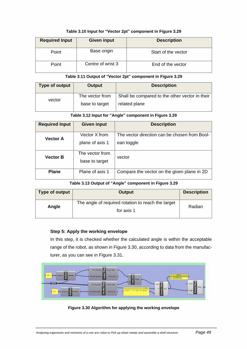
Analysing trajectories and moments of a one arm robot to Pick up sheet metals and assemble a shell structure Page 49
Table 3.10 Input for “Vector 2pt” component in Figure 3.29
Required Input Given input Description
Point Base origin Start of the vector
Point Centre of wrist 3 End of the vector
Table 3.11 Output of “Vector 2pt” component in Figure 3.29
Type of output Output Description
vector The vector from
base to target
Shall be compared to the other vector in their
related plane
Table 3.12 Input for “Angle” component in Figure 3.29
Required Input Given input Description
Vector A Vector X from
plane of axis 1
The vector direction can be chosen from Bool-
ean toggle
Vector B The vector from
base to target vector
Plane Plane of axis 1 Compare the vector on the given plane in 2D
Table 3.13 Output of “Angle” component in Figure 3.29
Type of output Output Description
Angle The angle of required rotation to reach the target
for axis 1 Radian
Step 5: Apply the working envelope
In this step, it is checked whether the calculated angle is within the acceptable
range of the robot, as shown in Figure 3.30, according to data from the manufac-
turer, as you can see in Figure 3.31.
Figure 3.30 Algorithm for applying the working envelope

Analysing trajectories and moments of a one arm robot to Pick up sheet metals and assemble a shell structure Page 50
Figure 3.31 Working envelope for axis 1
Step 6: Orient the related element of axis 1
According to the rotation angle, which was found in the previous step, the element
related to axis 1 is oriented to the identified direction. The critical component in
this step is the “Orient” component which is explained in Table 3.14 and Table
3.15. The implementation in Grasshopper can be found in Figure 3.32 and a vis-
ualization of the output in Figure 3.33.
Figure 3.32 algorithm to find the final position of axis 1
Table 3.14 Input of Orient component
Required Input Given input Description
Geometry YZ plane related to axis two at the joint point Geometry
Source Axis 1 Plane before rotation Plane
Target Axis 1 Plane after rotation Plane
Table 3.15 Output of Orient component
Type of output Output Description
Geometry Reoriented geometry Transformation data

Analysing trajectories and moments of a one arm robot to Pick up sheet metals and assemble a shell structure Page 51
Figure 3.33 Initial and final position of element 1
Step 7: Define the plane for axis 2
As shown in Figure 3.35, the plane for axis 2 consists of x and z-axis of axis 1 to
get to the position of axis 2 influenced by the transformation the axis 1.
Figure 3.34 algorithm to find axis two according to the rotation of axis 1
Figure 3.35 New position of axis two according to the rotation of axis 1

Analysing trajectories and moments of a one arm robot to Pick up sheet metals and assemble a shell structure Page 52
Step 8: Find the position of wrist 1
Figure 3.36 shows how to find possible wrist positions by creating two circles in
the plane of axis 2. To determine the possible wrist positions, two circles are
created to show the working envelope of wrist 1 and wrist 3 and to identify the
possible position of the end of the arm.
Figure 3.36 algorithm for finding the possible position of wrist 1
Step 9: Find the rotation angle of axis 2
The purpose of this step is to create a vector from the joint center to the intersec-
tion point which are found in step 8 and to calculate the angle between those
vectors and the z-axis of axis 2. There are two points resulting from the intersec-
tion of working radius of wrist 1 and wrist 3. Therefore, two vectors can be gen-
erated and there are two possible positions of wrist 1. As shown in Figure 3.37,
a Boolean toggle is used to select between two positions by changing the value
of Boolean from false to true. A visualization of the output is given in Figure 3.38.
Figure 3.37 Algorithm for applying the working envelope

Analysing trajectories and moments of a one arm robot to Pick up sheet metals and assemble a shell structure Page 53
Figure 3.38 Calculation of angle between position vector and z-axis
Step 10: Apply the working envelope
In this step, the found angle is checked, whether it is in the acceptable range of
the robot, as shown in Figure 3.39. The acceptable range is given by the manu-
facturer. Figure 3.40 gives a short overview about the range of the chosen robot.
Figure 3.39 Algorithm for applying the working envelope
Figure 3.40 Working envelope for axis 2 (KUKA Roboter GmbH 2016)

Analysing trajectories and moments of a one arm robot to Pick up sheet metals and assemble a shell structure Page 54
Step 11: Orient the related element to axis 2
According to the rotation angle which is found in the previous step, the element
related to axis 2 is oriented to the found direction. As shown in Figure 3.41, the
“Orient” component is applied the same way as it is explained in Table 3.14 and
Table 3.15. Figure 3.42 visualizes the output within Rhino.
Figure 3.41 Algorithm for orienting the element to the final position
Figure 3.42 Orient the robot element to the final position
Step12: Find the rotation angle of axis 3
In this part, the x-axis of the base plane needs to be compared with the vector
from the base plane to origin of the target plane. This is necessary to determine
the rotation angle of the base plane in order to reach the direction of the target
plane. The implementation in Grasshopper is shown in Figure 3.43 and the result
of this step within Rhino in Figure 3.44.
Figure 3.43 Algorithm for finding the plane related to axis 3

Analysing trajectories and moments of a one arm robot to Pick up sheet metals and assemble a shell structure Page 55
Figure 3.44 Orient the plane of axis 3
Step 13: Apply the working envelope
In the algorithm shown in Figure 3.45, the calculated angle is checked, whether
it is in the acceptable range of the robot according to data from the manufacturer.
Figure 3.46 gives an overview of the specifications of the manufacturer.
Figure 3.45 Algorithm for applying the working envelope
Figure 3.46 Working envelope for axis 3 (KUKA Roboter GmbH 2016)
Step 14: Orient the robot element according to the found in the last step
According to the calculated rotation angle, the element related to axis 1 is ori-
ented to the determined direction. As shown in Figure 3.41, the “Orient” compo-
nent is applied the same way as it is explained in Table 3.14 and Table 3.15.
Figure 3.42 visualizes the output in Rhino.

Analysing trajectories and moments of a one arm robot to Pick up sheet metals and assemble a shell structure Page 56
Figure 3.47 Algorithm for Orienting the element to new position
Figure 3.48 Orient the element to new position
Step 15: Find the rotation angle of axis 4
The purpose of step 15 is to find the rotation angle of axis 4. The plane for axis 4
can be created by utilizing the y- and z-axis of the plane used for axis 3 . the
rotation angle is found by comparing to the z-axis of the target plane. Figure 3.49
shows the implementation in Grasshopper and Figure 3.50 the result in Rhino.
Figure 3.49 Algorithm for finding rotation angle of axis 4
Figure 3.50 creating the plane of axis 4 relatively to axis 3

Analysing trajectories and moments of a one arm robot to Pick up sheet metals and assemble a shell structure Page 57
Step 16: Orient the robot element according to the found in the last step
To orient, the related element of axis 4 , the same procedure as explained in step
14 shall be repeated. As shown in Figure 3.51, the “Orient” component is applied
the same way as it is explained in Table 3.14 and Table 3.15.
Figure 3.51 Algorithm for Orienting the element to new position
Figure 3.52 Orient the element related to axis 4
Step 17: Find the rotation angle of axis 5
The creation of the plane for axis 5 follows the same procedure as in step 14.
Therefore, the angle between the x-axis of the plane for axis 5 and the z-axis of
the target plane is calculated(Figure 3.53).
Figure 3.53 Algorithm for finding the rotation angle of axis 5

Analysing trajectories and moments of a one arm robot to Pick up sheet metals and assemble a shell structure Page 58
Figure 3.54 Defining the plane related to axis 5
Step 18: Apply the working envelope
In step shown in Figure 3.55, the calculated angle is checked, whether it is in the
acceptable range of the robot according to data from the manufacturer. Figure
3.40 gives an overview of the specifications of the manufacturer.
Figure 3.55 Apply the working envelope to axis 5
Related element to axis 5 is oriented as same as step 15.
Figure 3.56 Orient the element related to axis 5 to final position
Figure 3.57 Final position of axis 5

Analysing trajectories and moments of a one arm robot to Pick up sheet metals and assemble a shell structure Page 59
Step 19: Find the rotation angle of axis 6
To find the angle of rotation of axis 6, the y-axis of the target plane is compared
with the x-axis vector of target plane, as shown in Figure 3.59 and the related
element is oriented as shown in Figure 3.61.
Figure 3.58 Algorithm for finding the rotation angle of axis 6
Figure 3.59 Visual description of the method for finding the angle of axis 6
Figure 3.60 Orient the related element to the final position
Figure 3.61 Orient the element related to axis 6 to the final position

Analysing trajectories and moments of a one arm robot to Pick up sheet metals and assemble a shell structure Page 60
Step 20: Analyzing the output
The output of the algorithm is the angle value for each joint. The algorithm finds
all possible positions for the Boolean toggles which is explained in previous steps.
If the selected position is not reachable by the robot, the algorithm will show which
axis is not in the reachable domain, as shown in yellow boxes in Figure 3.62.
Figure 3.62 Output of Inverse kinematic algorithm
Figure 3.63 Output of inverse kinematic algorithm
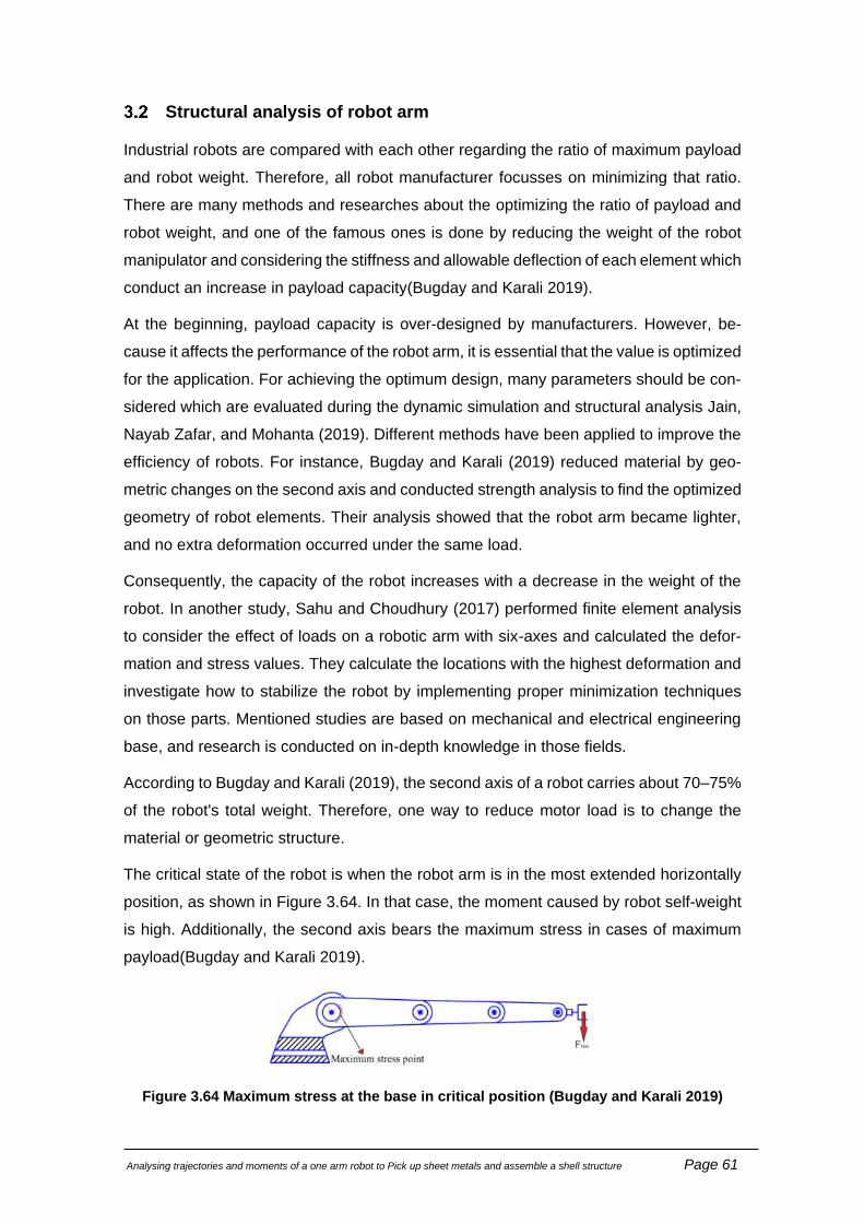
Analysing trajectories and moments of a one arm robot to Pick up sheet metals and assemble a shell structure Page 61
Structural analysis of robot arm
Industrial robots are compared with each other regarding the ratio of maximum payload
and robot weight. Therefore, all robot manufacturer focusses on minimizing that ratio.
There are many methods and researches about the optimizing the ratio of payload and
robot weight, and one of the famous ones is done by reducing the weight of the robot
manipulator and considering the stiffness and allowable deflection of each element which
conduct an increase in payload capacity(Bugday and Karali 2019).
At the beginning, payload capacity is over-designed by manufacturers. However, be-
cause it affects the performance of the robot arm, it is essential that the value is optimized
for the application. For achieving the optimum design, many parameters should be con-
sidered which are evaluated during the dynamic simulation and structural analysis Jain,
Nayab Zafar, and Mohanta (2019). Different methods have been applied to improve the
efficiency of robots. For instance, Bugday and Karali (2019) reduced material by geo-
metric changes on the second axis and conducted strength analysis to find the optimized
geometry of robot elements. Their analysis showed that the robot arm became lighter,
and no extra deformation occurred under the same load.
Consequently, the capacity of the robot increases with a decrease in the weight of the
robot. In another study, Sahu and Choudhury (2017) performed finite element analysis
to consider the effect of loads on a robotic arm with six-axes and calculated the defor-
mation and stress values. They calculate the locations with the highest deformation and
investigate how to stabilize the robot by implementing proper minimization techniques
on those parts. Mentioned studies are based on mechanical and electrical engineering
base, and research is conducted on in-depth knowledge in those fields.
According to Bugday and Karali (2019), the second axis of a robot carries about 70–75%
of the robot's total weight. Therefore, one way to reduce motor load is to change the
material or geometric structure.
The critical state of the robot is when the robot arm is in the most extended horizontally
position, as shown in Figure 3.64. In that case, the moment caused by robot self-weight
is high. Additionally, the second axis bears the maximum stress in cases of maximum
payload(Bugday and Karali 2019).
Figure 3.64 Maximum stress at the base in critical position (Bugday and Karali 2019)

Analysing trajectories and moments of a one arm robot to Pick up sheet metals and assemble a shell structure Page 62
Considering all these conditions, research focuses on increasing the capacity, the work-
ing radius of the robot. The first aspect can be achieved by redefining the pick point of
the payload. Figure 3.65 shows an overview of the workflow for the structural analysis of
the robot.
Figure 3.65 Overview of the algorithm for structural analysis of robot
3.2.1 Minimizing the moment and assign weight to elements
In this part, an algorithm that is developed to assign weight to elements and minimize
the moment in each joint of the robot arm is demonstrated. The primary purpose of the
algorithm is to integrate robotic movement for automated picking point selection of pan-
els. In summary, the geometrical data of the selected panel is imported to the algorithm
and is evaluated for possible picking points. On top, the best point that leads to lower
moments in joints is selected.
Figure 3.66 shows the geometry of a sample panel which is used as input for the target
plane in the inverse kinematic algorithm. The purpose of this algorithm is to find the best
picking point and use it as the origin point of the target plane. The target plane is utilized
as input for the inverse kinematic algorithm.
Figure 3.66 Geometry of sample panel
The algorithm for assigning weight to the panel is shown in Figure 3.67. Calculating the
weight of the panel is done by using the “Volume” component and using the definition of
density. The weight of the panel is calculated and shown in the yellow box in the algo-
rithm which is shown in Figure 3.67.
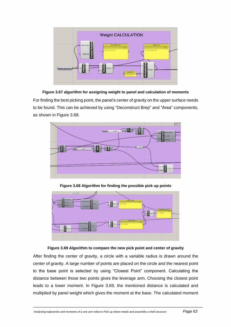
Analysing trajectories and moments of a one arm robot to Pick up sheet metals and assemble a shell structure Page 63
Figure 3.67 algorithm for assigning weight to panel and calculation of moments
For finding the best picking point, the panel’s center of gravity on the upper surface needs
to be found. This can be achieved by using “Deconstruct Brep” and “Area” components,
as shown in Figure 3.68.
Figure 3.68 Algorithm for finding the possible pick up points
Figure 3.69 Algorithm to compare the new pick point and center of gravity
After finding the center of gravity, a circle with a variable radius is drawn around the
center of gravity. A large number of points are placed on the circle and the nearest point
to the base point is selected by using “Closest Point” component. Calculating the
distance between those two points gives the leverage arm. Choosing the closest point
leads to a lower moment. In Figure 3.69, the mentioned distance is calculated and
multiplied by panel weight which gives the moment at the base. The calculated moment

Analysing trajectories and moments of a one arm robot to Pick up sheet metals and assemble a shell structure Page 64
value is compared with the moment of the normal position of the picking point. The result
shows that changing the pick point leads to 15 % lower moment. Now, it is necessary to
check the stability of the robot for the selected pick point and load, which is explained in
the next part.

Analysing trajectories and moments of a one arm robot to Pick up sheet metals and assemble a shell structure Page 65
3.2.2 Check the robot stability
Many parameters shall be considered to check the stability of the robot, as explained in
part 3.2. According to Figure 3.3, the robot datasheet and working instruction of the robot
which is prepared during the design process, the stability of robot is related to the dis-
tance of the center of forces to end effector flange. Therefore, it is necessary to know
the approximate shape of the gripper to calculate the mentioned distance.
According to Monkman and Hesse (2009), a good gripper shall be designed as below:
• Optimum adjustment of the gripper structure to the operations performed.
• Large adjustment range and options to grabbed parts of different shape and size.
• Reliability with respect to dislocations of the object (stability of the object position
and orientation).
• Optimum gripping force path characteristics.
• A low number of links and joints (where applicable).
• Small installation space and mass, robustness.
• High reliability combined with secure service.
• Avoidance of damage and deformation to the object during prehension.
According to the classification of the gripper in Figure 3.71, a magnetic gripper is a good
option for assembling sheet metal panels of a shell structure. After evaluating a lot of
magnetic gripper manufacturers, the average extended dimension which needs to be
considered in addition to the end effector flange is around 20 cm which is considered in
the algorithm in Figure 3.70.
Figure 3.70 Algorithm for checking the stability of the robot

Analysing trajectories and moments of a one arm robot to Pick up sheet metals and assemble a shell structure Page 66
The algorithm in Figure 3.70 is calculating the distance between the center of forces in
the z-direction and XY plane according to the payload diagram (see Figure 3.3 ). Also, it
is necessary to check if the momentum produced by the payload exceeds the maximum
allowed moment at the base point. The result of the analysis appears in the green box
in the algorithm(see Figure 3.70).
Figure 3.71 Gripper classification (Monkman and Hesse 2009)

Analysing trajectories and moments of a one arm robot to Pick up sheet metals and assemble a shell structure Page 67
Tracking trajectory of installation of critical elements of shell structure
panels
After evaluating different cases and principles of robotics as well as recent research in-
terest in the industry and academia, a holistic approach to Robotic Assembly Prototyping
in Grasshopper is developed. This methodology is used for a project with an assembly
orientated robotic setup using sheet metals with a pre-assigned assembly sequence in
Grasshopper. The core challenge is to achieve the integration of picking, placing, and
fitting the components of a structure. In this research, the KUKA KR1000 industrial robot
arm is used to run the assembly process. The components are cut by laser and brought
to the assembly site.
The algorithm for this chapter contains three important parts as shown in Figure 4.1.
Figure 4.1 Algorithm for assembly panels by the robot
The geometry of the critical cross-section shell structure model
A dome structure is selected as an example of a shell structure which is composed of
sheet metal panels. In order to create panels to shape a dome, the basics of tessellations
are used through grasshopper plugins. Tessellations subdivide a surface into a mesh of
simple elements such as triangles or Voronoi (Bailly et al. 2014). For this purpose, the
dimension of the structure is 2.8*3 meters with a height of 3 meters at the peak point of
the dome. In this research, some part of the whole structure is only studied for critical
elements and can be applied to the rest of the structure. After determining the general
dimensions of the structure, the boundaries of the structure are defined as explained in
Table 4.1 and Table 4.2:

Analysing trajectories and moments of a one arm robot to Pick up sheet metals and assemble a shell structure Page 68
Figure 4.2 Creating the geometry of the dome
Table 4.1 Input for Arc 3Pt component
Required Input Given input Description
3 Points 3 points from base to the highest point of the dome point
Table 4.2 Output for Arc 3Pt component
Type of output Output Description
Polyline Half cross-section of the structure polyline
Moreover, the shape of the dome is identified by rotating the mentioned line in Figure
4.2 by 360 °. The details of the algorithm are shown in Figure 4.3 and explained in Ta-
ble 4.3 and Table 4.4. The visualization of the output is shown in Figure 4.4.
Figure 4.3 General form of the dome
Table 4.3 Input for Revolution component
Required Input Given input Description
Curve Created polyline from Arc 3Pt component Profile curve
Axis The vector from 0 positions and in the di-
rection of Z-axis Revolution axis
Domain 0 to 2Pi Angle domain (in ra-dians)
Rotation axis
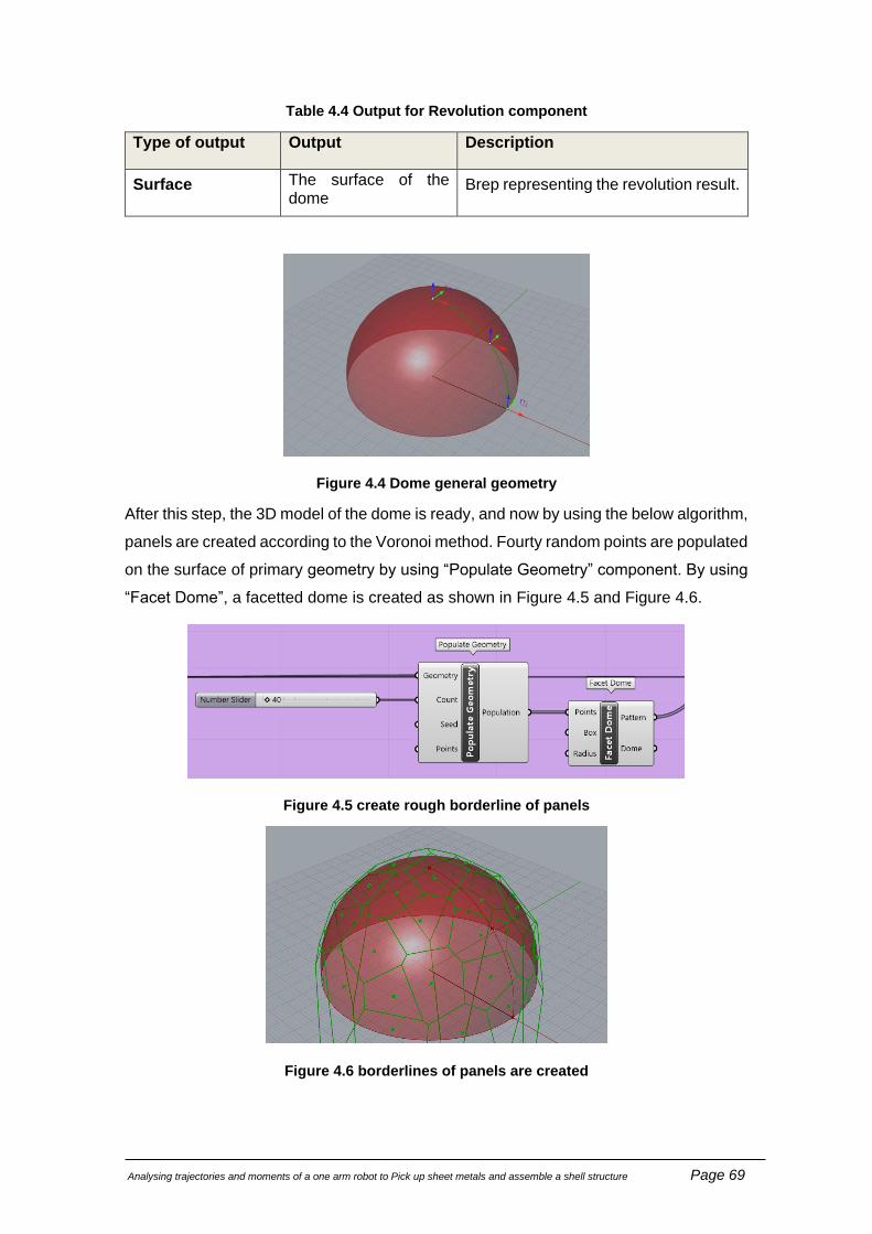
Analysing trajectories and moments of a one arm robot to Pick up sheet metals and assemble a shell structure Page 69
Table 4.4 Output for Revolution component
Type of output Output Description
Surface The surface of the dome
Brep representing the revolution result.
Figure 4.4 Dome general geometry
After this step, the 3D model of the dome is ready, and now by using the below algorithm,
panels are created according to the Voronoi method. Fourty random points are populated
on the surface of primary geometry by using “Populate Geometry” component. By using
“Facet Dome”, a facetted dome is created as shown in Figure 4.5 and Figure 4.6.
Figure 4.5 create rough borderline of panels
Figure 4.6 borderlines of panels are created

Analysing trajectories and moments of a one arm robot to Pick up sheet metals and assemble a shell structure Page 70
To make the panels smoother and create a better visual view of the dome “Pull Curve”
component is used to pull the curve from Facet dome onto the dome surface. The result
in Rhino is shown in Figure 4.8.
Figure 4.7 projecting the curve from facet dome on the curved surface of the dome
Figure 4.8 projected curve on the dome surface
Now, the borders of each panel are created. In the next step, the curves should be
changed to panels using components which are explained in Table 4.5 to Table 4.8:
Figure 4.9 Create panels as surface

Analysing trajectories and moments of a one arm robot to Pick up sheet metals and assemble a shell structure Page 71
Table 4.5 Input for Explode component
Required Input Given input Description
Curve Curve from Pull curve component Curve to explode
Table 4.6 Output for Explode component
Type of output Output Description
Vertices Start and endpoint of each edge
of panels
Vertices of the exploded seg-
ments
Table 4.7 Input for Patch component
Required Input Given input Description
Crvs Curves from polyline component Edge curves defining the patch
Table 4.8 Output for Patch component
Type of output Output Description
Patch Panel geometry A patch surface (Generic data)
The output of this step gives the geometry and size of each panel, including each edge
of the panel and area as below:
Figure 4.10 Output of form-finding algorithm

Analysing trajectories and moments of a one arm robot to Pick up sheet metals and assemble a shell structure Page 72
Simulation and analysis of assembly process using KUKA|PRC
In this part, possible scenarios for the position of the robot and assembly process are
investigated. The construction phase of the shell structure starts with the preparation of
a final surface which is necessary to be able to use the robot on site. The second step is
the transport of the robots to the site. Setting up the robot and disassembly processes of
heavy load industrial robots are time-consuming processes. The calibration of the robot
makes the process even more complex. Therefore, using mobile robots in order to work
on site is necessary. However, based on what is discussed in chapter 1 and chapter 2,
in order to use mobile robots on site more development and technical improvement are
required. An alternative for a mobile robot is to use rails so that the robot can move on
an additional axis. On the market, this is known as a linear unit. There are many types
and models of these tracks available on the market which has a wide range of length
and payload. In this study, because a KUKA robot is chosen, the KUKA linear unit
KR3000 is suggested for the on-site assembly process. The length of KUKA KL 3000
can be extended to 30 m. A general view of this track line is shown in Figure 4.11.
Figure 4.11 KUKA Linear unit KL3000
One possible plan for assembling the panels is to divide the dome into two parts and to
place the linear unit in the middle (Figure 4.12). In this case, linear units shall be disas-
sembled once to change the position of robot for assembling the other half of dome. The

Analysing trajectories and moments of a one arm robot to Pick up sheet metals and assemble a shell structure Page 73
middle rib is the connection between both of the “half domes” should be installed manu-
ally after disassembling the linear unit.
Figure 4.12 Locating robot between two parts of the dome for assembly
The second possible solution is to assemble the panels from outside of the dome. Eval-
uation of robot’s movement shows that the curved dome structure makes it a complex
task to reach all placing points for assembly. Therefore, to assemble all panels, the linear
unit shall be moved three times according to Figure 4.13. Changing the position of the
linear unit is the most suitable option in comparison to using multiple robots because
using multiple robots is more expensive and transporting more than one robot restrict
the flexibility on the construction site.
Figure 4.13 Locating robot outside of the structure for assembly

Analysing trajectories and moments of a one arm robot to Pick up sheet metals and assemble a shell structure Page 74
4.2.1 Tracking trajectory of assembly of critical elements
After the structure’s form has been found and the creation of all panels, the structure is
ready for construction. The purpose of this part is to investigate the assembly process of
critical panels of the shell structure. Five panels are selected, as shown in Figure 4.14.
The panels which are close to the ground make the assembly process more complex
because the slope of the panels is steeper and the robot's movement is limited for those
areas.
Figure 4.14 five critical panels for the assembly process is selected
The diagram in Figure 4.15 shows the general overview of the assembly process as a
cycle for one element. This task will be repeated for all elements.
Figure 4.15 robot path for assembly cycle
START
MOVE TO SAFETY
DISTANCE pick up position
Grab the panel
move the element to safety distance
moving and orienting the endeffector
Move to the safety distance of
prepositioing point
the panel mounted on its position
the end effector goes to safety
distance
Go to Next Element pick
position

Analysing trajectories and moments of a one arm robot to Pick up sheet metals and assemble a shell structure Page 75
In this section, the programming process of each stage will be discussed to explain the
grasshopper algorithm. According to the assembly process, shown in Figure 4.15, the
coordinates of each point needs to be determined as the point placed in a specified
plane. This will be used as robot input in the next steps. Therefore, in the following steps,
we are looking for the proper point and plane orientation which robot uses as origin and
destination for each movement.
The algorithm shown in Figure 4.16 is the section for defining the trajectory to simulate
the assembly process of the five mentioned panels by KUKA robots using KUKA PRC
plugin in Grasshopper. The algorithm consists of four main parts, defining pick up point,
final position and safety planes for each position.
Figure 4. An overview of the algorithm for assembly
To set up the site for better performance of the robot, panels are placed on a table which
is shown in Figure 4.17. Because the robot’s performance improves when the payload
is picked up above ground level.
Figure 4.16 Assembly site setting
Define pickup plane
Define safety plane
Define final position plane
Define safety plane

Analysing trajectories and moments of a one arm robot to Pick up sheet metals and assemble a shell structure Page 76
In the first step, the panels are oriented on the delivery table by using the “Orient” com-
ponent shown in Table 4.9. The robot's end-effector should be moved to a picking point,
which is calculated according to the algorithm in chapter three. The pickup points are
selected for each panel on the delivery table.
Table 4.9 Final position of elements
Input Orient Output
Geometry
(Geometry)
Base ge-
ometry
Geometry (Geometry)
Reoriented geometry Source
(Plane)
Initial plane
Target
(Plane)
Final plane
Transform (Transform)
Transformation data
Compo-
nent's fea-
ture:
Orient an object. Orientation is sometimes called a 'Change Basis
transformation'. It allows for remapping of geometry from one axis-sys-
tem to another.
After defining the picking point, we move the point 60 cm upwards in a vertical
direction to provide safety, as shown in Figure 4.17.
Figure 4.17 Finding safety plane
After finding the final position of the whole element it is necessary to find the placing
points. The placing point is the location of the robot where the element can be placed.

Analysing trajectories and moments of a one arm robot to Pick up sheet metals and assemble a shell structure Page 77
Because the picking point and the final position of the panels are found in a way that
they are related to each other, this ensures that the final position of the element matches
the position specified in the 3D-model. The same procedure of finding a safety plane is
performed to find the safety plane 60 cm perpendicular to the panels and in the opposite
direction of the panels.
As shown in Figure 4.19, all relevant points and planes are found. Afterward, the assem-
bly process can be defined by using the KUKA PRC plugin and by using correctly ori-
ented planes on each position.
Figure 4.18 Points of each step's position
KUKA PRC plugin is a tool which helps to simulate the movement of the robot's end-
effector in Rhino. For starting the simulation, we need to use the “KUKA|prc CORE” com-
ponent shown in Table 4.10. This component contains all core functionality such as sim-
ulation and code generation.
As a first step, we need to define movement commands as an input for the “KUKA|prc
CORE” component. The plugin provides different types of movement which are demon-
strated in Table 4.10.

Analysing trajectories and moments of a one arm robot to Pick up sheet metals and assemble a shell structure Page 78
Table 4.10 KUKA PRC CORE
Input KUKA PRC CORE Output
Simulation Slider (Number)
Number slider ranging from 0.0
to 1.0 for controlling the simula-
tion position. The values are
normalised in that range, taking
the movement speed and calcu-
lated total time into account.
Robot Geometry
(Geometry)
A series of meshes
showing the current
position of the robot.
Bake it, e.g. for visu-
alisation and render-
ing.
Commands (KUKA|prc Com-
mand)
A series of KUKA|prc Com-
mands (e.g. LINear, PTP, AXIS
movements) that define the ro-
bot's toolpath.
Tool (KUKA|prc Tool Data)
Optional. Tool definition provid-
ing the properties and geometry
of the attached tool. If no tool is
connected, the simulation will
assume a tool number of 0 and
0,0,0,0,0,0 as XYZABC values. Analysis Output
(KUKA|prc Analysis
Data)
In-depth access to
the simulation values
is provided through
the separate
KUKA|prc Analysis
component.
Robot (KUKA|prc Robot Data)
Robot definition providing the
kinematic properties and geom-
etry of the robot.
KUKA|prc Collision Geometry
(Mesh)
Optional. A series of meshes
that define collision geometry.
Enable collision checking in the
KUKA|prc settings. Note that
collision checking has got a
large, negative impact on
KUKA|prc performance.
Component's feature: KUKA|prc core component containing all core functionality
such as simulation and code generation.
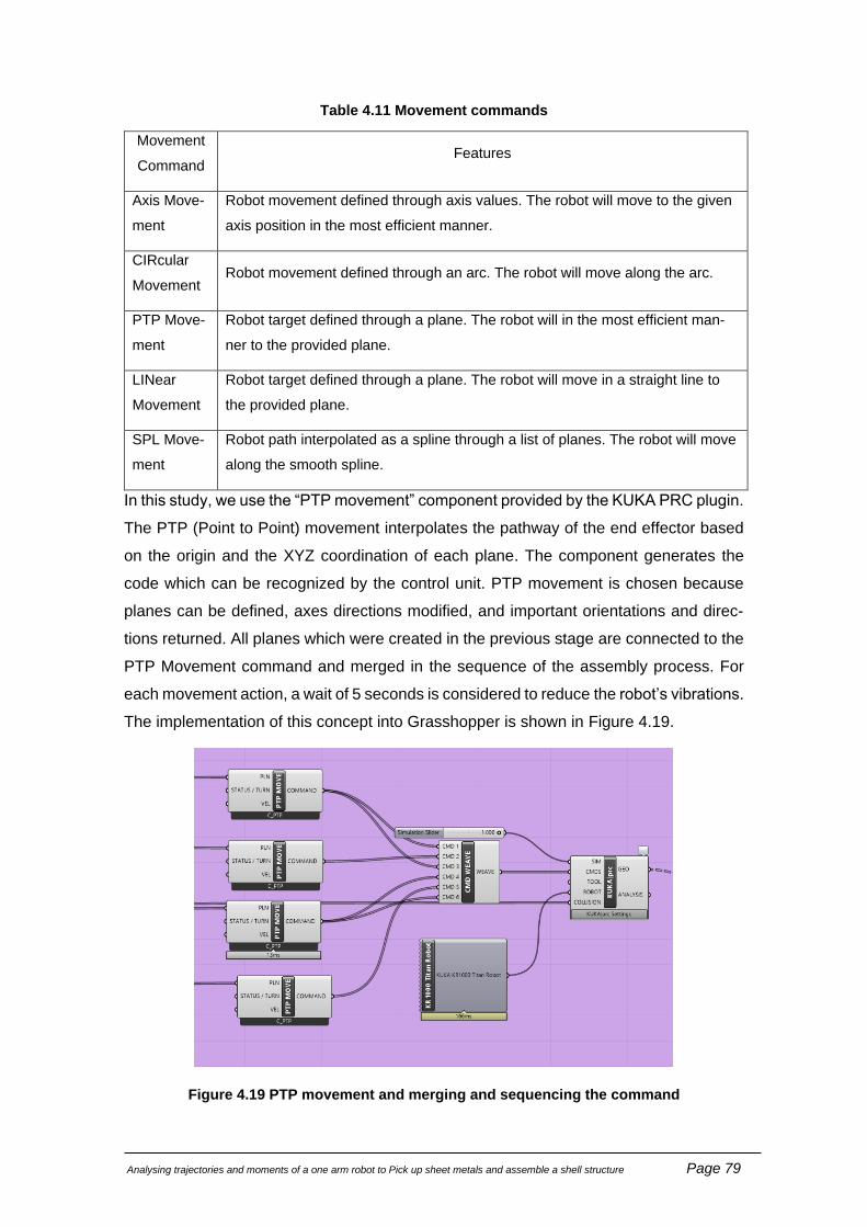
Analysing trajectories and moments of a one arm robot to Pick up sheet metals and assemble a shell structure Page 79
Table 4.11 Movement commands
Movement
Command Features
Axis Move-
ment
Robot movement defined through axis values. The robot will move to the given
axis position in the most efficient manner.
CIRcular
Movement Robot movement defined through an arc. The robot will move along the arc.
PTP Move-
ment
Robot target defined through a plane. The robot will in the most efficient man-
ner to the provided plane.
LINear
Movement
Robot target defined through a plane. The robot will move in a straight line to
the provided plane.
SPL Move-
ment
Robot path interpolated as a spline through a list of planes. The robot will move
along the smooth spline.
In this study, we use the “PTP movement” component provided by the KUKA PRC plugin.
The PTP (Point to Point) movement interpolates the pathway of the end effector based
on the origin and the XYZ coordination of each plane. The component generates the
code which can be recognized by the control unit. PTP movement is chosen because
planes can be defined, axes directions modified, and important orientations and direc-
tions returned. All planes which were created in the previous stage are connected to the
PTP Movement command and merged in the sequence of the assembly process. For
each movement action, a wait of 5 seconds is considered to reduce the robot’s vibrations.
The implementation of this concept into Grasshopper is shown in Figure 4.19.
Figure 4.19 PTP movement and merging and sequencing the command

Analysing trajectories and moments of a one arm robot to Pick up sheet metals and assemble a shell structure Page 80
KUKA PRC plugin prepares the Programmable logic controller (PLC) code according to
the type of robot. This code can be exported as.txt format and can be imported to a KUKA
controller on-site to control the robot. Alternatively, the user can choose the desired
platform provided by this plugin, e. g. KUKA SUNRISE, KUKA KRL and KUKA CAMROB
are choosable. Figure 4.21 shows the graphical user interface of the KUKA|prc plugin,
Figure 4.22 gives an example code and Figure 4.23 shows the robot during the assembly
process.
Figure 4.20 KUKA PRC Output
Figure 4.21 Output of KUKA PRC

Analysing trajectories and moments of a one arm robot to Pick up sheet metals and assemble a shell structure Page 81
Figure 4.22 Robot during the assembly process
4.2.2 Discuss obstacles and clash detection
This part discusses the assembly process of the most critical elements. A crucial stage
in each robot orientated project is the collision checking. For example, robots arms pro-
vide exact sensors to avoid accidents with the environment. Aside from the environmen-
tal collision checking, collision between the element carried by the robot and other ele-
ments should be checked. In this research, the assembly process of the most extended
element is analyzed. The collision check is done manually by frame by frame analyses
of the simulation. Wherever a collision happens, the orientation of the plane or the coor-
dination of its origin is changed.
The diagram in Figure 4.23 is generated by KUKA PRC and shows a robot with six axes.
It shows the axes value during the simulation period. If there is any wrist collision, the
yellow color will be shown on the diagram. In case the position is out of reach, the dia-
gram shows a red area. A simulation is accurate when there is no red area. In this case,
all results are trustable, and no collision happened.
Figure 4.23 Analysis result
Safety plane
Safety plane
Pick up plane
Final position
plane

Analysing trajectories and moments of a one arm robot to Pick up sheet metals and assemble a shell structure Page 82
After making sure that all axes of robot are able to perform the required maneuvers dur-
ing the assembly process step by step visual analysis of the collision checking is done.
Figure 4.24 to Figure 4.34demonstrate this process. The critical point is when the robot
approaches the final position of each panel, therefore those points are investigated, and
special protection and supervision is needed during assembly on site. Each step was
evaluated precisely and when a collision happened, the defined angle of joints has been
modified to get the collision-free workflow. The result of this part shows that planning of
assembly process needs much attention and the process shall be monitored by sensors
to avoid any collision because robot should execute many maneuvers to find the right
orient and final position of panels.
Figure 4.24 Robot picks the first panel
Figure 4.25 Robot assembles the first panel
Figure 4.26 Robot picks the second panel
Figure 4.27 Robot assembles the second panel
Figure 4.28 Robot picks the third panel
Figure 4.29 Robot assembles the third panel

Analysing trajectories and moments of a one arm robot to Pick up sheet metals and assemble a shell structure Page 83
Figure 4.30 Robot picks the fourth panel
Figure 4.31 Robot assembles the fourth panel
Figure 4.32 Robot picks the fifth panel
Figure 4.33 Robot assembles the fifth panel
Figure 4.34 Assembly process finished

Analysing trajectories and moments of a one arm robot to Pick up sheet metals and assemble a shell structure Page 84
Conclusions and Future Work
Conclusions
Modern architecture is focusing on free forms. It conducts customization in architectural
design which causes complex and unique components. Computer-aided architectural
design has been developed as a digital model to fabricate high volumes at a reasonable
cost, referred to as mass customization. It allows architectural forms to be parametrically
controlled, resulting in an automatic generation of design variants or overall design man-
agement. This research work uses Rhino and Grasshopper to show the concept of par-
ametric design of free forms.
Conventional construction methods are not compatible with the freeform building; ac-
cordingly, unique methods need to be used, which are uneconomical and consume a
high volume of material. Recently, robotic assembly and fabrication are receiving more
attention from researchers. Experts in robotic fabrication and computational geometry
have explored new possibilities for including robotic assembly and material selection into
the process. The main idea to facilitate working with robots is to integrate design, fabri-
cation, and building assembly is by considering the robot constraints and abilities. The
case studies show that the use of robots for the fabrication of architectural element has
incredibly developed when compared to the use of robots in construction. In this context,
research about the possibilities to increase the use of robotic arms in construction is
presented. This concept integrates different cases of using robots for customized man-
ufacturing and construction.
One of the objectives of this research work is to model line diagrams of the robotic arm
(KUKA titan 1000). Analysis and simulation tools are one of the important tools to con-
ceptualize the use of robots in construction. There are many plug-ins and components
in Grasshopper mostly focusing on path planning and collision detection for milling, 3D
printing and winding. These plug-ins have limitations in modelling the payloads and an-
alyzing the effect of payload and end effector on the robot.
The model of the robot is developed according to control methods. The forward kinematic
model is capable to find the final position of the end effector based on the given values
of joints, but it is not efficient for path planning. Therefore, the second model is developed
based on inverse kinematic. This model finds the joints value according to the target
plane. The results show that the inverse kinematic model is suitable for path planning
and tracking the trajectories.

Analysing trajectories and moments of a one arm robot to Pick up sheet metals and assemble a shell structure Page 85
The environmental situation of construction sites is different from fabrication plants. In
fabrication plants, robots are planned to execute repetitive tasks with almost similar pay-
loads but on construction sites, the robot’s task is unique with different payloads. There-
fore, integrating the path planning and defining the trajectories with structural analysis
may lead to improved robotic performance on construction sites. Grasshopper and Rhino
do not support finite element analysis for given geometries. In addition, most of the plug-
ins are developed for the analysis of structural elements and limited for analyzing of
robots. Therefore, the second objective of the thesis is to develop an algorithm for struc-
tural analysis of the robot. An algorithm is developed to define the weight of the payload
according to the input data and it is integrated with the inverse kinematic model. In in-
dustry, robots are planned to pick the elements from the center of gravity. In this case,
the size of the panels is wide. Therefore, the center of gravity of panels may be far from
the end effector and picking the panels from the center of gravity results in limitations.
Therefore, the algorithm finds the best pick point which leads to minimizing the moment
at the base. The comparison of different pick points shows a 15 percent decrease in the
moment. In addition , the research shows that the gripper plays a key role in handling of
the payload and it is assumed that the proper gripper for panels is selected.
In the next part of the thesis, a dome is designed and panelized according to Voronoi
method. Panels have different shape and size. Thus, this model contains many unique
elements which can be a good prototype for simulating and analyzing the assembly pro-
cesses of a shell structure using a robotic arm. Evaluating different scenarios of assem-
bly processes shows that using a mobile robot is necessary due to limited working range
of fixed robots. On the other hand, construction sites are not stable and they change day
by day and it is hard for mobile robots to integrate with the environment. Therefore, the
use of mobile robots on construction site is limited due to lack of technology hence mobile
robots are underdeveloped. This research suggests using linear tracks which gives the
robots the ability of linear movement. The results show that dividing the dome into two
parts and place the linear track in between is the most efficient approach.
The research continues with breaking down the trajectory of the robot arm for assembling
the critical panels of the dome. Robot movement is restricted for moving panels which
should be placed at a low level. Therefore. five panels are selected and the assembly
plan is designed which is applicable for other panels. In this process, safety distance is
considered to get more accuracy and also between each step of the assembly process,
wait command is used to help robot being stabilized. The developed model can be used
as a reference workflow for all panels. The trajectory and end-effector pathway are mod-
elled in Grasshopper and analyzed and modified to avoid any collision.

Analysing trajectories and moments of a one arm robot to Pick up sheet metals and assemble a shell structure Page 86
Thus, it can be concluded that constructing a panelized shell structure using a robot arm
is successful. However, improving the assembly processes needs the contribution of
engineers from different fields, i.e., mechanic and electronic. Moreover, it is understood
that automation can be applied from the very first steps of the project. Manufacturable
panels can be generated during the architectural design process. Robots can execute
the manufacturing process of the panels and also assembling those on construction site.
Future Work
This research work illustrates that using a robot on construction sites needs more devel-
opment for various applications, as it is a multidisciplinary approach and needs cooper-
ation between engineers of different fields such as electronics, mechanics, construction,
and architecture. This research work can be extended in various aspects as mentioned
below:
• For structural analysis of robots, the most accurate method is finite element anal-
ysis. The mentioned analysis in this study for the design process is time-consum-
ing. To address this challenge, a study on the implementation of plugins for par-
ametric finite element analysis shall be considered.
• The role of gripper in handling of panels with different shape is very important.
There are many types of gripper in market to help humans in moving and handling
of large and heavy elements. Study on utilizing industrial magnetic gripper on
robotic arms can be done as extend of this research work.
• Since mobile robots need a considerable number of sensors to carry out activities
on the construction site, a study shall be carried out on methods to increase the
interaction of robot adapting to different activities and construction sites.
• To make the simulation and analysis more practical and realistic, an interactive
algorithm is beneficial by extending and developing the algorithm for receiving
data from force sensors of the robot and use as input for analysis.
• Exploration of more shell structure designs to get the most compatible geometry
with robotic construction.

Analysing trajectories and moments of a one arm robot to Pick up sheet metals and assemble a shell structure Page 87
Bibliography
Aktas, Kerim Gökhan, Fatih Pehlivan, and İsmail Esen. 2017. “Kinematic Analysis of 4
Degrees of Freedom Robotic Arm and Simultaneous Trajectory Tracking Using
ADAMS®-MATLAB® Software.”
Bailly, D., M. Bambach, G. Hirt, T. Pofahl, R. Herkrath, H. Heyden, and M. Trautz. 2014.
“Manufacturing of Innovative Self-Supporting Sheet-Metal Structures Representing
Freeform Surfaces.” Procedia CIRP 18:51–56.
Braumann, Johannes, and Sigrid Brell-Cokcan. 2011. “Parametric Robot Control:
Integrated CAD/CAM for Architectural Design.” Integration Through Computation -
Proceedings of the 31st Annual Conference of the Association for Computer Aided
Design in Architecture, ACADIA 2011 242–51.
Bugday, Mustafa, and Mehmet Karali. 2019. “Design Optimization of Industrial Robot
Arm to Minimize Redundant Weight.” Engineering Science and Technology, an
International Journal 22(1):346–52.
Dörfler, Kathrin, Timothy Sandy, Markus Giftthaler, Fabio Gramazio, Matthias Kohler,
and Jonas Buchli. 2016. “Mobile Robotic Brickwork.” Pp. 204–17 in Robotic
Fabrication in Architecture, Art and Design 2016. Cham: Springer International
Publishing.
El-Sherbiny, Ahmed, Mostafa A. Elhosseini, and Amira Y. Haikal. 2018. “A Comparative
Study of Soft Computing Methods to Solve Inverse Kinematics Problem.” Ain
Shams Engineering Journal 9(4):2535–48.
Gupta, Vaibhav, Rajeevlochana G. Chittawadigi, and Subir Kumar Saha. 2017. “Robo
Analyzer: Robot Visualization Software for Robot Technicians.” ACM International
Conference Proceeding Series Part F1320.
Hadid, Zaha. 2007. “Innsbruck Hungerburgbahn.” Retrieved June 1, 2020
(https://cz.pinterest.com/pin/349732727305361587/).
Helm, Volker, Selen Ercan, Fabio Gramazio, and Matthias Kohler. 2012. “Mobile Robotic
Fabrication on Construction Sites: DimRob.” Pp. 4335–41 in 2012 IEEE/RSJ
International Conference on Intelligent Robots and Systems. IEEE.
Jain, Rishabh, Mohd Nayab Zafar, and J. C. Mohanta. 2019. “Modeling and Analysis of
Articulated Robotic Arm for Material Handling Applications.” IOP Conference
Series: Materials Science and Engineering 691(1).
Jung, Alexander, Dagmar Reinhardt, and Rod Watt. 2016. “RBDM_Robodome: Complex

Analysing trajectories and moments of a one arm robot to Pick up sheet metals and assemble a shell structure Page 88
Curved Geometries with Robotically Fabricated Joints.” Pp. 178–89 in Robotic
Fabrication in Architecture, Art and Design 2016. Cham: Springer International
Publishing.
KUKA Roboter GmbH. 2016. “Spez KR 1000 Titan V8.” Pub Spez KR 1000 Titan En.
Retrieved April 13, 2020 (https://www.kuka.com/-/media/kuka-
downloads/imported/48ec812b1b2947898ac2598aff70abc0/spez_kr_1000_titan_e
n.pdf?modified=-1156406340).
Li, Rita Yi Man, and Rita Yi Man Li. 2018. “Robots for Construction Industry.” An
Economic Analysis on Automated Construction Safety 32–33.
Mark W. Spong, Seth Hutchinson, and M. Vidyasagar. 2008. Robot Dynamics And
Control. second. Wiley.
Monkman, Gareth J., and Stefan Hesse. 2009. Robot Grippers. Vol. 29.
Monkman, Gareth J., Stefan Hesse, Ralf Steinmann, and Henrik Schunk. 2006. Robot
Grippers. Wiley.
Monkman, Gareth J., Stefan Hesse, Ralf Steinmann, and Henrik Schunk. 2007.
“Introduction to Prehension Technology.” Robot Grippers 1–17.
Naboni, Roberto. 2015. SPRINGER BRIEFS IN APPLIED SCIENCES AND Advanced
Customization in Architectural Design and Construction.
Pottmann, Helmut. 2010. “Architectural Geometry as Design Knowledge.” Architectural
Design 80(4):72–77.
Pottmann, Helmut. 2013. “Architectural Geometry and Fabrication-Aware Design.”
Nexus Network Journal 15(2):195–208.
Sahu, Supriya, and B. B. Choudhury. 2017. “STATIC ANALYSIS OF A 6-AXIS
INDUSTRIAL ROBOT USING FINITE ELEMENT ANALYSIS.” International Journal
of Mechanical Engineering and Technology (IJMET) 8(3):49–55.
Schwartz, Mathew, and Jaeheung Park. 2017. “Robotic Control Strategies Applicable to
Architectural Design.” Technology Architecture and Design 1(1):73–82.
Sciavicco, Lorenzo, and Bruno Siciliano. 2000. Modelling and Control of Robot
Manipulators. London: Springer London.
Sousa, Pedro, Cristina Gass, Eduardo Moreira, Andry Maykol Pinto, Jos Lima, Paulo
Costa, Pedro Costa, Germano Veiga, and A. Paulo Moreira. 2016. “Robotic
Fabrication in Architecture, Art and Design 2016.” Robotic Fabrication in
Architecture, Art and Design 2016 231–39.

Analysing trajectories and moments of a one arm robot to Pick up sheet metals and assemble a shell structure Page 89
Sroka-Bizoń, Monika. 2016. “Architectural Geometry.”
Sullivan, Adam. 2014. “Robots, Drones, and Printed Buildings: The Promise of
Automated Construction.” Retrieved May 20, 2020
(https://www.bdcnetwork.com/robots-drones-and-printed-buildings-promise-
automated-construction).
Tatarnikov, Denis A. 2019. “Forward Kinematics.”
Wu, Kaicong, and Axel Kilian. 2016. “Robotic Fabrication in Architecture, Art and Design
2016.” Robotic Fabrication in Architecture, Art and Design 2016 241–49.
Wu, Kaicong, and Axel Kilian. 2020. “Designing Compression-Only Arch Structures
Using Robotic Equilibrium Assembly.” Pp. 608–22 in Impact: Design With All
Senses. Cham: Springer International Publishing.
Yang, Nian, Leilei Chen, Kheirollah Sepahvand, Hong Yi, and Steffen Marburg. 2017.
“Structural-Acoustic Optimization Based on Fast Multipole Boundary Element
Method Sensitivity Analysis of a Coupled Acoustic Fluid-Structure System.” The
Journal of the Acoustical Society of America 141(5):3513–3513.

Analysing trajectories and moments of a one arm robot to Pick up sheet metals and assemble a shell structure Page 90
Appendix
This is a digital appendix and following files are copied on the CD is attached :
A1: Line diagrams of robot according to forward and inverse kinematic in Rhino and
Grasshopper
A2: Algorithm for structural analysis of the robot
A3: Algorithm for tracking trajectories of assembly process