Embed Size (px)
Citation preview

ANALYSING UNCERTAINTY AND DELAYS
IN AIRCRAFT HEAVY MAINTENANCE
A thesis submitted to The University of Manchester
for the degree of Doctor of Philosophy
in the Faculty of Humanities
2015
Leandro Julian Salazar Rosales
Alliance Manchester Business School
Volume I of II

2
List of contents
Volume I of I I .................................................................................................. 1
List of contents .................................................................................................... 2
List of tables ........................................................................................................ 7
List of figures..................................................................................................... 13
Abstract ............................................................................................................. 18
Declaration ........................................................................................................ 19
Copyright Statement ......................................................................................... 19
Acknowledgments ............................................................................................. 20
List of abbreviations .......................................................................................... 21
Chapter 1: Introduction ..................................................................................... 23
1.1 Research motivation ................................................................................................... 27
1.2 Research questions .................................................................................................... 28
1.3 Research objectives .................................................................................................... 29
1.4 Empirical data .............................................................................................................. 30
1.5 Thesis structure ........................................................................................................... 30
Chapter 2: Context and description of the problem ........................................... 32
2.1 Influence and challenges of the airline industry. ......................................................... 32
2.2 Aircraft maintenance ................................................................................................... 34
2.2.1 The aim of aircraft maintenance ............................................................................... 35
2.2.2 Relevance of aircraft maintenance ........................................................................... 35
2.2.3 Structure of aircraft maintenance ............................................................................. 37
2.3 Aircraft heavy maintenance process ........................................................................... 41
2.3.1 Managing resources in heavy maintenance ............................................................. 42
2.3.2 Scheduling and planning heavy maintenance checks ............................................. 44
2.3.3 Heavy maintenance challenges ............................................................................... 46
2.4 Summary ..................................................................................................................... 47

3
Chapter 3: Literature review .............................................................................. 49
3.1 Aircraft maintenance planning, scheduling and management .................................... 49
3.1.1 Maintenance planning and scheduling ..................................................................... 49
3.1.2 Workforce planning and scheduling ......................................................................... 53
3.1.3 Management and supply of parts ............................................................................. 55
3.1.4 Process improvement ............................................................................................... 55
3.2 Project management ................................................................................................... 59
3.2.1 Project ....................................................................................................................... 60
3.2.2 Complex project ........................................................................................................ 60
3.2.3 Risk ........................................................................................................................... 62
3.2.4 Risk management ..................................................................................................... 63
3.2.5 Relevant approaches in project management .......................................................... 64
3.3 Uncertainty .................................................................................................................. 66
3.3.1 Classification of uncertainty ...................................................................................... 67
3.4 Alternative uncertainty theories ................................................................................... 69
3.4.1 Fuzzy set theory ....................................................................................................... 69
3.4.2 Evidence theory ........................................................................................................ 69
3.4.3 Possibility theory ....................................................................................................... 71
3.5 Simulation .................................................................................................................... 71
3.5.1 System ...................................................................................................................... 73
3.5.2 Model ........................................................................................................................ 74
3.6 System Dynamics (SD) ............................................................................................... 75
3.6.1 System dynamics in project management ................................................................ 77
3.7 Discrete Event Simulation (DES) ................................................................................ 80
3.8 Comparison of system dynamics and discrete event simulation ................................ 82
3.9 Summary ..................................................................................................................... 84
Chapter 4: Methodology and research design .................................................. 87
4.1 Ontological and epistemological basis of the research ............................................... 87
4.2 Research design ......................................................................................................... 90
4.3 System dynamics modelling ........................................................................................ 92
4.3.1 Causal loop diagrams ............................................................................................... 93

4
4.3.2 Stock and flow diagrams .......................................................................................... 94
4.3.3 System dynamics equations ..................................................................................... 96
4.3.4 Validation .................................................................................................................. 97
4.4 Evidential Reasoning rule ........................................................................................... 99
4.4.1 Dependency between the pieces of evidence ........................................................ 101
4.5 Operationalisation of the research questions ............................................................ 102
4.6 Summary ................................................................................................................... 103
Chapter 5: Analysing delays and disruptions in aircraft heavy maintenance
using System Dynamics ...................................................................... 105
5.1 Model articulation ...................................................................................................... 106
5.1.1 Model boundaries ................................................................................................... 106
5.1.2 Simulation software ................................................................................................ 106
5.1.3 Data collection ........................................................................................................ 107
5.2 Conceptual model development ................................................................................ 109
5.2.1 Understanding delays and disruptions in aircraft heavy maintenance process ..... 109
5.2.2 Integrating workforce, parts and materials, and tools and equipment ................... 115
5.3 Quantitative models .................................................................................................. 118
5.3.1 Analysing scheduled and unscheduled maintenance tasks ................................... 118
5.3.2 Managing maintenance scheduled tasks ............................................................... 127
5.4 Model validation ........................................................................................................ 141
5.5 Summary ................................................................................................................... 142
Chapter 6: Estimation of unscheduled maintenance tasks using the
Evidential Reasoning rule ................................................................... 144
6.1 Data and variables description .................................................................................. 145
6.2 Data statistical analysis ............................................................................................. 147
6.3 Data discretisation ..................................................................................................... 149
6.3.1 Determining the number of intervals and their width .............................................. 150
6.3.2 Intervals meaningfulness ........................................................................................ 153
6.3.3 Data distribution ...................................................................................................... 154
6.4 ER rule model ............................................................................................................ 155
6.4.1 Impact of limits and size of interval on model performance ................................... 165

5
6.4.2 Impact of different number of variables combined ................................................. 169
6.5 ER rule scenarios ...................................................................................................... 173
6.5.1 All pieces of evidence are independent, fully reliable and highly important ........... 173
6.5.2 All pieces of evidence are fully reliable, highly important and their dependency
is adjusted............................................................................................................... 174
6.5.3 All pieces of evidence are highly important, their dependency is adjusted and
they are not fully reliable ......................................................................................... 175
6.5.4 All pieces of evidence are not fully reliable and their importance and
dependency are adjusted ....................................................................................... 177
6.6 Sensitivity analysis of reliability ................................................................................. 179
6.6.1 Alpha index has been optimised, weight is one and the reliability of one piece
of evidence changes. .............................................................................................. 179
6.6.2 Alpha index has been optimised, weight is one and reliability is the same for all
pieces of evidence. ................................................................................................. 180
6.6.3 Reliability is the same for all pieces of evidence, weight and Alpha index are
equal to one and then optimised. ........................................................................... 181
6.7 Validation ................................................................................................................... 185
6.8 Summary ................................................................................................................... 187
Chapter 7: Discussion and conclusions .......................................................... 189
7.1 Empirical and theoretical grounding .......................................................................... 189
7.2 Models summary ....................................................................................................... 192
7.3 Research findings...................................................................................................... 194
7.3.1 Additional findings .................................................................................................. 197
7.4 Research limitations .................................................................................................. 198
7.5 Suggestions for future research ................................................................................ 200
7.6 Conclusions ............................................................................................................... 201
References...................................................................................................... 203
Volume II of I I : Appendixes ................................................................... 219
List of contents of Volume II ............................................................................ 220
Appendix A: SD models ............................................................................... 221
A.1 Conceptual model ..................................................................................................... 221

6
Appendix B: ER rule results ......................................................................... 229
B.1 Main data-set ............................................................................................................. 229
B.2 Variables frequency distribution ................................................................................ 232
B.3 Results of the ER rule model example ...................................................................... 237
B.4 Bin size and interval limits analysis ........................................................................... 242
B.5 Bin size layouts ......................................................................................................... 258
B.6 Number of predictor variables analysis ..................................................................... 258
B.7 ER rule model scenarios adjusting alpha index, reliability and weight ..................... 261
B.7.1 Optimised alpha-index results ................................................................................ 262
B.7.2 Optimised weights results ....................................................................................... 298
B.8 Sensitivity analysis results ........................................................................................ 302
B.8.1 Sensitivity analysis when the reliability of one variable is modified at a time ......... 302
B.8.2 Sensitivity analysis when the reliability of all variables is modified equally at the
same time ............................................................................................................... 312
B.8.3 Sensitivity analysis modifying alpha-index, weight and reliability........................... 315
B.9 Validation results ....................................................................................................... 325
Total word count excluding appendixes: 85,120
Total word count from introduction to conclusions: 71,760

7
List of tables
Table 5-1 Experts profile ........................................................................................................... 107
Table 6-1 Descriptive statistics of the main variables ............................................................... 148
Table 6-2 Relative frequency of heavy maintenance checks ................................................... 148
Table 6-3 Correlation between the variables ............................................................................ 149
Table 6-4 Number of intervals “k” and bin-widths “h” according to different rules. ................... 153
Table 6-5 Proposed number of intervals and bin-widths .......................................................... 154
Table 6-6 Non-routine rate frequency distribution of each piece of evidence .......................... 156
Table 6-7 Prior probabilities and likelihoods of each piece of evidence ................................... 157
Table 6-8 Non-routine rate belief distribution of each piece of evidence .................................. 158
Table 6-9 ER Rule for an aeroplane aged 6-8, with 3,250-3,500 fh/y, 1500-1750 cy/y and
a 4C service. ................................................................................................................... 160
Table 6-10 Expected non-routine rate belief distribution for the real combinations.................. 162
Table 6-11 Bin-width and intervals options for each variable ................................................... 165
Table 6-12 Model performance using different numbers of variables ...................................... 170
Table 6-13 Model performance when the variables are independent, fully reliable and highly
important. ........................................................................................................................ 174
Table 6-14 Model performance when the variables are not completely independent, but are
fully reliable and highly important. .................................................................................. 175
Table 6-15 Model performance when the variables are not completely independent and
reliable, but are highly important. .................................................................................... 177
Table 6-16 Model performance when the variables are not completely independent, reliable
and important. ................................................................................................................. 178
Table B-1 Main variables for building the ER rule model .......................................................... 229
Table B-2 Aircraft’s age frequency distributions considering different bin-widths and interval
limits ................................................................................................................................ 232
Table B-3 Flight hours per year frequency distributions considering different bin-widths and
interval limits ................................................................................................................... 234
Table B-4 Cycles per year frequency distributions considering different bin-widths and
interval limits ................................................................................................................... 235

8
Table B-5 Non-routine rate frequency distributions considering different bin-widths and
interval limits ................................................................................................................... 236
Table B-6 Comparison between Non-routine rate real distribution and Estimated Non-
routine rate belief distribution .......................................................................................... 237
Table B-7 Comparison between Real Non-routine rate and Estimated average Non-routine
rate .................................................................................................................................. 239
Table B-8 Model performance comparison for different bin-widths of flight and cycles per
year; considering interval-widths of 0.05 for non-routine rate and 0.5 for aircraft’s
age, with 4.5 and 13.0 years as lower and upper limits. ................................................. 242
Table B-9 Model performance comparison for different bin-widths of flight and cycles per
year; considering interval-widths of 0.05 for non-routine rate and 1.0 for aircraft’s
age, with 4.0 and 13.0 years as lower and upper limits. ................................................. 243
Table B-10 Model performance comparison for different bin-widths of flight and cycles per
year; considering interval-widths of 0.05 for non-routine rate and 1.0 for aircraft’s
age, with 4.5 and 13.5 years as lower and upper limits. ................................................. 244
Table B-11 Model performance comparison for different bin-widths of flight and cycles per
year; considering interval-widths of 0.05 for non-routine rate and 1.5 for aircraft’s
age, with 4.0 and 13.0 years as lower and upper limits. ................................................. 245
Table B-12 Model performance comparison for different bin-widths of flight and cycles per
year; considering interval-widths of 0.05 for non-routine rate and 1.5 for aircraft’s
age, with 4.5 and 13.5 years as lower and upper limits. ................................................. 246
Table B-13 Model performance comparison for different bin-widths of flight and cycles per
year; considering interval-widths of 0.05 for non-routine rate and 2.0 for aircraft’s
age, with 3.0 and 13.0 years as lower and upper limits. ................................................. 247
Table B-14 Model performance comparison for different bin-widths of flight and cycles per
year; considering interval-widths of 0.05 for non-routine rate and 2.0 for aircraft’s
age, with 4.0 and 14.0 years as lower and upper limits. ................................................. 248
Table B-15 Model performance comparison for different bin-widths of flight and cycles per
year; considering interval-widths of 0.05 for non-routine rate and 2.5 for aircraft’s
age, with 2.5 and 15.0 years as lower and upper limits. ................................................. 249
Table B-16 Model performance comparison for different bin-widths of flight and cycles per
year; considering interval-widths of 0.10 for non-routine rate and 0.5 for aircraft’s
age, with 4.5 and 13.0 years as lower and upper limits. ................................................. 250
Table B-17 Model performance comparison for different bin-widths of flight and cycles per
year; considering interval-widths of 0.10 for non-routine rate and 1.0 for aircraft’s
age, with 4.0 and 13.0 years as lower and upper limits. ................................................. 251

9
Table B-18 Model performance comparison for different bin-widths of flight and cycles per
year; considering interval-widths of 0.10 for non-routine rate and 1.0 for aircraft’s
age, with 4.5 and 13.5 years as lower and upper limits. ................................................. 252
Table B-19 Model performance comparison for different bin-widths of flight and cycles per
year; considering interval-widths of 0.10 for non-routine rate and 1.5 for aircraft’s
age, with 4.0 and 13.0 years as lower and upper limits. ................................................. 253
Table B-20 Model performance comparison for different bin-widths of flight and cycles per
year; considering interval-widths of 0.10 for non-routine rate and 1.5 for aircraft’s
age, with 4.5 and 13.5 years as lower and upper limits. ................................................. 254
Table B-21 Model performance comparison for different bin-widths of flight and cycles per
year; considering interval-widths of 0.10 for non-routine rate and 2.0 for aircraft’s
age, with 3.0 and 13.0 years as lower and upper limits. ................................................. 255
Table B-22 Model performance comparison for different bin-widths of flight and cycles per
year; considering interval-widths of 0.10 for non-routine rate and 2.0 for aircraft’s
age, with 4.0 and 14.0 years as lower and upper limits. ................................................. 256
Table B-23 Model performance comparison for different bin-widths of flight and cycles per
year; considering interval-widths of 0.10 for non-routine rate and 2.5 for aircraft’s
age, with 2.5 and 15.0 years as lower and upper limits. ................................................. 257
Table B-24 Layout A interval array ........................................................................................... 258
Table B-25 Layout B interval array ........................................................................................... 258
Table B-26 Layout A: Model performance comparison excluding one predictor variable ........ 258
Table B-27 Layout B: Model performance comparison excluding one predictor variable ........ 258
Table B-28 Layout A: Model performance comparison excluding two predictor variables ....... 259
Table B-29 Layout B: Model performance comparison excluding two predictor variables ....... 259
Table B-30 Layout A: Model performance comparison excluding three predictor variables .... 260
Table B-31 Layout B: Model performance comparison excluding three predictor variables .... 260
Table B-32 Layout A (Four samples): Model performance comparison adjusting Alpha
index, Reliability and Weight ........................................................................................... 261
Table B-33 Layout B (Four samples): Model performance comparison adjusting Alpha
index, Reliability and Weight ........................................................................................... 261
Table B-34 Layout A, Sample A: Optimised alpha-index per non-routine rate for combining
aeroplane age and flight hours per year ......................................................................... 262
Table B-35 Layout A, Sample A: Optimised alpha-index per non-routine rate for combining
aeroplane age and flight hours per year with cycles per year ........................................ 263

10
Table B-36 Layout A, Sample A: Optimised alpha-index per non-routine rate for combining
aeroplane age, flight hours and cycles per year with service type ................................. 265
Table B-37 Layout A, Sample B: Optimised alpha-index per non-routine rate for combining
aeroplane age and flight hours per year ......................................................................... 268
Table B-38 Layout A, Sample B: Optimised alpha-index per non-routine rate for combining
aeroplane age and flight hours per year with cycles per year ........................................ 269
Table B-39 Layout A, Sample B: Optimised alpha-index per non-routine rate for combining
aeroplane age, flight hours and cycles per year with service type ................................. 271
Table B-40 Layout A, Sample C: Optimised alpha-index per non-routine rate for combining
aeroplane age and flight hours per year ......................................................................... 274
Table B-41 Layout A, Sample C: Optimised alpha-index per non-routine rate for combining
aeroplane age and flight hours per year with cycles per year ........................................ 275
Table B-42 Layout A, Sample C: Optimised alpha-index per non-routine rate for combining
aeroplane age, flight hours and cycles per year with service type ................................. 277
Table B-43 Layout A, Sample D: Optimised alpha-index per non-routine rate for combining
aeroplane age and flight hours per year ......................................................................... 280
Table B-44 Layout A, Sample D: Optimised alpha-index per non-routine rate for combining
aeroplane age and flight hours per year with cycles per year ........................................ 281
Table B-45 Layout A, Sample D: Optimised alpha-index per non-routine rate for combining
aeroplane age, flight hours and cycles per year with service type ................................. 283
Table B-46 Layout B, Sample A: Optimised alpha-index per non-routine rate for combining
aeroplane age and flight hours per year ......................................................................... 286
Table B-47 Layout B, Sample A: Optimised alpha-index per non-routine rate for combining
aeroplane age and flight hours per year with cycles per year ........................................ 286
Table B-48 Layout B, Sample A: Optimised alpha-index per non-routine rate for combining
aeroplane age, flight hours and cycles per year with service type ................................. 287
Table B-49 Layout B, Sample B: Optimised alpha-index per non-routine rate for combining
aeroplane age and flight hours per year ......................................................................... 289
Table B-50 Layout B, Sample B: Optimised alpha-index per non-routine rate for combining
aeroplane age and flight hours per year with cycles per year ........................................ 289
Table B-51 Layout B, Sample B: Optimised alpha-index per non-routine rate for combining
aeroplane age, flight hours and cycles per year with service type ................................. 290
Table B-52 Layout B, Sample C: Optimised alpha-index per non-routine rate for combining
aeroplane age and flight hours per year ......................................................................... 292

11
Table B-53 Layout B, Sample C: Optimised alpha-index per non-routine rate for combining
aeroplane age and flight hours per year with cycles per year ........................................ 292
Table B-54 Layout B, Sample C: Optimised alpha-index per non-routine rate for combining
aeroplane age, flight hours and cycles per year with service type ................................. 293
Table B-55 Layout B, Sample D: Optimised alpha-index per non-routine rate for combining
aeroplane age and flight hours per year ......................................................................... 295
Table B-56 Layout B, Sample D: Optimised alpha-index per non-routine rate for combining
aeroplane age and flight hours per year with cycles per year ........................................ 295
Table B-57 Layout B, Sample D: Optimised alpha-index per non-routine rate for combining
aeroplane age, flight hours and cycles per year with service type ................................. 296
Table B-58 Layout A (Four samples): Optimised weights for each piece of evidence ............. 298
Table B-59 Layout B (Four samples): Optimised weights for each piece of evidence ............. 300
Table B-60 Layout A, Sample A: Sensibility analysis when alpha index has been optimised,
weight is one and the reliability of one variable is modified at a time ............................. 302
Table B-61 Layout A, Sample B: Sensibility analysis when alpha index has been optimised,
weight is one and the reliability of one variable is modified at a time ............................. 303
Table B-62 Layout A, Sample C: Sensibility analysis when alpha index has been optimised,
weight is one and the reliability of one variable is modified at a time ............................. 304
Table B-63 Layout A, Sample D: Sensibility analysis when alpha index has been optimised,
weight is one and the reliability of one variable is modified at a time ............................. 305
Table B-64 Layout A (Four samples): MAI when alpha index has been optimised, weight is
one and the reliability of one variable is modified at a time ............................................ 306
Table B-65 Layout B, Sample A: Sensibility analysis when alpha index has been optimised,
weight is one and the reliability of one variable is modified at a time ............................. 307
Table B-66 Layout B, Sample B: Sensibility analysis when alpha index has been optimised,
weight is one and the reliability of one variable is modified at a time ............................. 308
Table B-67 Layout B, Sample C: Sensibility analysis when alpha index has been optimised,
weight is one and the reliability of one variable is modified at a time ............................. 309
Table B-68 Layout B, Sample D: Sensibility analysis when alpha index has been optimised,
weight is one and the reliability of one variable is modified at a time ............................. 310
Table B-69 Layout B (Four samples): MAI when alpha index has been optimised, weight is
one and the reliability of one variable is modified at a time ............................................ 311
Table B-70 Layout A (Four samples): Sensibility analysis when alpha index has been
optimised, weight is one and the reliability of all variables is modified equally at the
same time ....................................................................................................................... 312

12
Table B-71 Layout B (Four samples): Sensibility analysis when alpha index has been
optimised, weight is one and the reliability of all variables is modified equally at the
same time ....................................................................................................................... 313
Table B-72 Layout A and B (Four samples): MAI when alpha index has been optimised,
weight is one and the reliability of all variables is modified equally at the same time .... 314
Table B-73 Layout A (Four samples): Sensibility analysis when alpha index is one, weight
is one and the reliability of all variables is modified equally at the same time................ 315
Table B-74 Layout A (Four samples): Sensibility analysis when alpha index is one, weight
is optimised and the reliability of all variables is modified equally at the same time ...... 316
Table B-75 Layout A (Four samples): Sensibility analysis when alpha index is optimised,
weight is one and the reliability of all variables is modified equally at the same time .... 317
Table B-76 Layout A (Four samples): Sensibility analysis when alpha index is optimised,
weight is optimised and the reliability of all variables is modified equally at the same
time ................................................................................................................................. 318
Table B-77 Layout A (Four samples): MAI comparison when alpha index and weight are
one and then optimised, and the reliability of all variables is modified equally at the
same time ....................................................................................................................... 319
Table B-78 Layout B (Four samples): Sensibility analysis when alpha index is one, weight
is one and the reliability of all variables is modified equally at the same ....................... 320
Table B-79 Layout B (Four samples): Sensibility analysis when alpha index is one, weight
is optimised and the reliability of all variables is modified equally at the same time ...... 321
Table B-80 Layout B (Four samples): Sensibility analysis when alpha index is optimised,
weight is one and the reliability of all variables is modified equally at the same time .... 322
Table B-81 Layout B (Four samples): Sensibility analysis when alpha index is optimised,
weight is optimised and the reliability of all variables is modified equally at the same
time ................................................................................................................................. 323
Table B-82 Layout B (Four samples): MAI comparison when alpha index and weight are
one and then optimised, and the reliability of all variables is modified equally at the
same time ....................................................................................................................... 324
Table B-83 Layout A: Model performance comparison of the training and validation groups
and all the dataset ........................................................................................................... 325
Table B-84 Layout B: Model performance comparison of the training and validation groups
and all the dataset ........................................................................................................... 326

13
List of figures
Figure 1-1 Causal loop diagrams, SD simulation model and ER rule model interaction ............ 25
Figure 2-1 2008 vs 2014 Comparison of Average Revenues and Net Profits per Passenger
(Source: IATA (2015b)). .................................................................................................... 33
Figure 2-2 Yearly Airline Industry Net Profit Margin (Sources: IATA (2009, 2015a, 2015b)).
.......................................................................................................................................... 34
Figure 2-3 Typical Direct Operating Costs Distribution - scheduled airlines ICAO member
states 2007 (Source: Doganis (2009)). ............................................................................. 37
Figure 2-4 Aircraft maintenance programme development ........................................................ 39
Figure 2-5 Line and heavy maintenance, and the elements required for an effective
maintenance process. Based on Aubin (2004, p.11). ....................................................... 41
Figure 2-6 Significance of Heavy maintenance for airlines and MROs ...................................... 42
Figure 2-7 Interrelationship between heavy maintenance resources. ........................................ 42
Figure 2-8 Delays and disruptions in the heavy maintenance process ...................................... 46
Figure 3-1 Basic uncertainty types (Klir and Wierman, 1999, p.103) ......................................... 68
Figure 4-1 Causal loop diagrams notation .................................................................................. 94
Figure 4-2 Causal loop diagram example: the dynamics of population. Based on (Sterman,
2000, p.138) ...................................................................................................................... 94
Figure 4-3 Stock and flow diagram notation ............................................................................... 95
Figure 4-4 Stock-flow diagram example: the dynamics of population. Based on (Sterman,
2000, p.285) ...................................................................................................................... 96
Figure 5-1 Qualitative data collection ........................................................................................ 108
Figure 5-2 Delays and disruptions in aircraft heavy maintenance process .............................. 110
Figure 5-3 Scheduled tasks and resources allocation .............................................................. 111
Figure 5-4 Occurrence and discovery of discrepancies ............................................................ 112
Figure 5-5 Unscheduled tasks and the fight for resources ....................................................... 113
Figure 5-6 Increase of available resources ............................................................................... 113
Figure 5-7 Extend the project deadline ..................................................................................... 115
Figure 5-8 Interrelationship between workforce, parts and materials, and tools and
equipment ....................................................................................................................... 116

14
Figure 5-9 Ways to increase workforce .................................................................................... 117
Figure 5-10 Ripple and knock-on effects of increasing workforce ............................................ 118
Figure 5-11 Occurrence and discovery of discrepancies .......................................................... 119
Figure 5-12 Workforce allocation .............................................................................................. 119
Figure 5-13 Discrepancies discovery distribution 1 .................................................................. 125
Figure 5-14 Discrepancies discovery distribution 2 .................................................................. 125
Figure 5-15 Routine and non-routine tasks (80% workforce allocated to routine) ................... 126
Figure 5-16 Routine and non-routine tasks (50% workforce allocated to routine).................... 126
Figure 5-17 Remaining tasks and project duration (different workforce allocation) .................. 127
Figure 5-18 Variable workforce allocation for routine tasks ...................................................... 127
Figure 5-19 Managing maintenance scheduled tasks .............................................................. 128
Figure 5-20 Remaining number of tasks per day (ideal conditions) ......................................... 138
Figure 5-21 Remaining number of tasks per day (with delays) ................................................ 138
Figure 5-22 Workforce allocation per day (ideal conditions) ..................................................... 139
Figure 5-23 Workforce allocation per day (with delays) ............................................................ 139
Figure 5-24 Project backlog (ideal conditions) .......................................................................... 140
Figure 5-25 Project backlog (with delays) ................................................................................. 140
Figure 5-26 Additional workforce required (ideal conditions) .................................................... 140
Figure 5-27 Additional workforce required (with delays) ........................................................... 141
Figure 6-1 Main variables for estimating the non-routine rate .................................................. 147
Figure 6-2 Scatterplot of non-routine rate by type of maintenance service .............................. 149
Figure 6-3 Aircraft's age frequency distribution with a bin-width of 0.5 years........................... 154
Figure 6-4 Aircraft's age frequency distribution with a bin-width of 2.0 years........................... 154
Figure 6-5 Aircraft's age frequency distribution with a bin-width of 1.5 year, lower limit 2.5 .... 155
Figure 6-6 Aircraft's age frequency distribution with a bin-width of 1.5 year, lower limit 3.0 .... 155
Figure 6-7 ER Rule for an aeroplane aged 6-8, with 3,250-3,500 fh/y, 1500-1750 cy/y and
a 4C service. ................................................................................................................... 161
Figure 6-8 MAE and MAPE comparison across scenarios using different bin size .................. 166
Figure 6-9 MAI for the 400 different combinations of interval arrays ........................................ 167
Figure 6-10 MAE and MAPE comparison across scenarios using different interval limits ....... 167

15
Figure 6-11 MAE and MAPE comparing two different arrays of intervals ................................ 168
Figure 6-12 Mean Accuracy Indicator considering different numbers of variables ................... 170
Figure 6-13 Mean Accuracy Indicator using four predictor variables ....................................... 171
Figure 6-14 Mean Accuracy Indicator using three predictor variables ..................................... 171
Figure 6-15 Mean Accuracy Indicator using two predictor variables ........................................ 172
Figure 6-16 Importance degree (weight value) for each piece of evidence .............................. 178
Figure 6-17 Model sensitivity when the reliability of one variable is modified, for layouts A
and B ............................................................................................................................... 180
Figure 6-18 Model sensitivity when the reliability of all variables is modified, for layouts A
and B ............................................................................................................................... 181
Figure 6-19 Model sensitivity when α=1, the reliability of all variables is modified and weight
is optimised, for layouts A and B .................................................................................... 182
Figure 6-20 Model sensitivity when α has been adjusted, the reliability of all variables is
modified and weight is optimised, for layouts A and B ................................................... 183
Figure 6-21 Model sensitivity comparison when α=1 and then is adjusted, and when
weight=1 and then is optimised, for layouts A and B ...................................................... 184
Figure 6-22 Importance degree (optimised weight values) for each piece of evidence for
different reliability values, for layouts A and B ................................................................ 185
Figure 6-23 MAI comparison for training and validation groups and for the whole sample ...... 186
Figure A-1 Scheduled tasks and resources allocation .............................................................. 221
Figure A-2 Occurrence and discovery of discrepancies ........................................................... 222
Figure A-3 Unscheduled tasks and the fight for resources ....................................................... 223
Figure A-4 Increase of available resources .............................................................................. 224
Figure A-5 Extend the project deadline ..................................................................................... 225
Figure A-6 Delays and disruptions in aircraft heavy maintenance process .............................. 226
Figure A-7 Ways to increase workforce .................................................................................... 227
Figure A-8 Ripple and knock-on effects of increasing workforce.............................................. 228
Figure B-9 Aircraft's age frequency distribution with a bin-width of 0.5 years and limits from
4 to 13.5 .......................................................................................................................... 232
Figure B-10 Aircraft's age frequency distribution with a bin-width of 1 year and limits from
3 to 14 ............................................................................................................................. 232

16
Figure B-11 Aircraft's age frequency distribution with a bin-width of 1 year and limits from
3.5 to 14.5 ....................................................................................................................... 232
Figure B-12 Aircraft's age frequency distribution with a bin-width of 1.5 years and limits
from 2.5 to 14.5 ............................................................................................................... 232
Figure B-13 Aircraft's age frequency distribution with a bin-width of 1.5 years and limits
from 3 to 15 ..................................................................................................................... 232
Figure B-14 Aircraft's age frequency distribution with a bin-width of 2 years and limits from
1 to 15 ............................................................................................................................. 233
Figure B-15 Aircraft's age frequency distribution with a bin-width of 2 years and limits from
2 to 16 ............................................................................................................................. 233
Figure B-16 Aircraft's age frequency distribution with a bin-width of 2.5 years and limits
from 0 to 17.5 .................................................................................................................. 233
Figure B-17 Flight hours/year frequency distribution: bin-width of 100FH and limits from
2,300 to 4,600 ................................................................................................................. 234
Figure B-18 Flight hours/year frequency distribution: bin-width of 150FH and limits from
2,150 to 4,700 ................................................................................................................. 234
Figure B-19 Flight hours/year frequency distribution: bin-width of 200FH and limits from
2,200 to 4,800 ................................................................................................................. 234
Figure B-20 Flight hours/year frequency distribution: bin-width of 250FH and limits from
2,000 to 4,750 ................................................................................................................. 234
Figure B-21 Flight hours/year frequency distribution: bin-width of 300FH and limits from
2,000 to 5,000 ................................................................................................................. 234
Figure B-22 Cycles/year frequency distribution: bin-width of 100Cy and limits from 800 to
2,700 ............................................................................................................................... 235
Figure B-23 Cycles/year frequency distribution: bin-width of 150Cy and limits from 750 to
2,700 ............................................................................................................................... 235
Figure B-24 Cycles/year frequency distribution: bin-width of 200Cy and limits from 600 to
3,000 ............................................................................................................................... 235
Figure B-25 Cycles/year frequency distribution: bin-width of 250Cy and limits from 500 to
3,000 ............................................................................................................................... 235
Figure B-26 Cycles/year frequency distribution: bin-width of 300Cy and limits from 600 to
3,000 ............................................................................................................................... 235
Figure B-27 Non-routine rate frequency distribution: bin-width of 0.025 and limits from 0.05
to 0.475 ........................................................................................................................... 236

17
Figure B-28 Non-routine rate frequency distribution: bin-width of 0.05 and limits from 0.0 to
0.55 ................................................................................................................................. 236
Figure B-29 Non-routine rate frequency distribution: bin-width of 0.10 and limits from 0.0 to
0.60 ................................................................................................................................. 236
Figure B-30 Layout A: Optimised weights for each piece of evidence ..................................... 299
Figure B-31 Layout B: Optimised weights for each piece of evidence ..................................... 301
Figure B-32 Layout A: MAI comparison for training and validation groups and for the whole
sample ............................................................................................................................ 325
Figure B-33 Layout B: MAI comparison for training and validation groups and for the whole
sample ............................................................................................................................ 326

18
Abstract
Analysing Uncertainty and Delays in Aircraft Heavy Maintenance
The University of Manchester
Leandro Julian Salazar Rosales
Doctor of Philosophy
December, 2015
This study investigates the influence of unscheduled maintenance activities on delays and disruptions during the execution of aircraft heavy maintenance services by developing a simulation model based on Systems Dynamics (SD) and supported by an Evidential Reasoning (ER) rule model.
The SD model studies the complex interrelationship between scheduled and unscheduled tasks and its impact on delays during a maintenance service execution. It was found that the uncertain nature of the unscheduled maintenance tasks hinders the planning, control and allocation of resources, increasing the chances to miss deadlines and incur in cost overruns. Utilising causal loop diagrams and SD simulation the research explored the relevance that the resource allocation management, the precise estimation of the unscheduled tasks and their prompt identification have on the maintenance check duration. The influence that delays and attitudes in the decision-making process have on project performance was also investigated.
The ER rule model investigates the uncertainty present during the execution of a maintenance check by providing a belief distribution of the expected unscheduled maintenance tasks. Through a non-parametric discretisation process, it was found that the size and array of distribution intervals play a key role in the model estimation accuracy. Additionally, a sensitivity analysis allowed the examination of the significance that the weight, reliability and dependence of the different pieces of evidence have on model performance. By analysing and combining historical data, the ER rule model provides a more realistic and accurate prediction to analyse variability and ambiguity.
This research extends SD capabilities by incorporating the ER rule for analysing system uncertainty. By using the belief distributions provided by the ER model, the SD model can simulate the variability of the process given certain pieces of evidence.
This study contributes to the existing knowledge in aircraft maintenance management by analysing, from a different perspective, the impact of uncertain unscheduled maintenance activities on delays and disruptions through an integrated approach using SD and the ER rule. Despite the fact that this research focuses on studying a particular problem in the airline industry, the findings and conclusions obtained could be used to understand and address problems embodying similar characteristics. Therefore, it can be argued that, due to the close similarities between the heavy maintenance process and complex projects, these contributions can be extended to the Project Management field.

19
Declaration
No portion of the work referred to in this thesis has been submitted in support of an application
for another degree or qualification of this or any other university or other institute of learning.
Copyright Statement
The following four notes on copyright and the ownership of intellectual property rights must be
included as written below:
1. The author of this thesis (including any appendices and/or schedules to this thesis) owns
certain copyright or related rights in it (the “Copyright”) and he has given The University of
Manchester certain rights to use such Copyright, including for administrative purposes.
2. Copies of this thesis, either in full or in extracts and whether in hard or electronic copy, may
be made only in accordance with the Copyright, Designs and Patents Act 1988 (as amended)
and regulations issued under it or, where appropriate, in accordance with licensing
agreements which the University has from time to time. This page must form part of any such
copies made.
3. The ownership of certain Copyright, patents, designs, trademarks and other intellectual
property (the “Intellectual Property”) and any reproductions of copyright works in the thesis,
for example graphs and tables (“Reproductions”), which may be described in this thesis, may
not be owned by the author and may be owned by third parties. Such Intellectual Property
and Reproductions cannot and must not be made available for use without the prior written
permission of the owner(s) of the relevant Intellectual Property and/or Reproductions.
4. Further information on the conditions under which disclosure, publication and
commercialisation of this thesis, the Copyright and any Intellectual Property and/or
Reproductions described in it may take place is available in the University IP Policy (see
http://documents.manchester.ac.uk/DocuInfo.aspx?DocID=487), in any relevant Thesis
restriction declarations deposited in the University Library, The University Library’s
regulations (see http://www.manchester.ac.uk/library/aboutus/regulations) and in The
University’s policy on Presentation of Theses.

20
Acknowledgments
First and foremost, I would like to thank my supervisor, Professor Jian-Bo Yang, whose vast
knowledge and experience, along with his invaluable and constant support, helped me throughout
the development of this research. His advice inspired me to develop the skills of a researcher and
encouraged me to pursue critical thinking. In particular, I also thank him for accepting me as part
of his recognised research team. I also want to express my gratitude to Dr Yu-Wang Chen, part
of this great research team and my co-supervisor, who has always been willing to help and guide
me whenever needed.
I would also like to thank the members of the Decision and Cognitive Sciences Research Group
(DCSRG) for the discussions and suggestions that helped me improve my research. I especially
appreciate the support of Dr Julia Handl and Professor Dong-Ling Xu for trusting me as Seminar
Leader of their courses.
I must also acknowledge the National Council of Science and Technology of Mexico (CONACYT)
for granting me a scholarship to pursue a PhD. Without its financial support, this project would
not have materialised.
It is also important to recognise the key role that my colleagues in the airline industry played in
the development of this work. Without their expertise and knowledge, it would not have been
possible to conduct this research.
During my PhD, I had the opportunity to meet extraordinary people who became my friends. Their
support and advice made the completion of this project possible. Thanks to Carlos Ramos,
Emanuel-Emil Savan and Raza Khan for always listening to my concerns with patience and
understanding. I also want to thank Tom Jenks for his proofreading work but particularly for his
continuous and priceless help.
I especially want to thank my wife, Marisol, for encouraging me during this adventure and for her
limitless help and patience. Without her, I would have not been able to complete this endeavour.
I also want to thank my little girl, Silvana, who inadvertently motivated me to keep on going in the
final stages of this research. Finally, I want to thank all my family, particularly my parents, for all
the support and love that I have received, and my family in-law who have always been there for
me as true parents and siblings.

21
List of abbreviations
AHP Analytical Hierarchy Process
APM Association for Project Management
ARP Aircraft Routing Problem
AWL Airworthiness Limitations
BD Belief Distribution
BS British Standard
CAA Civil Aviation Authority, UK
CCM Critical Chain Method
CLD Causal Loop Diagram
CMR Certification Maintenance Requirements
CPM Critical Path Method
CY Flight Cycles per Year
DEA Data Envelopment Analysis
DES Discrete Event Simulation
DOT Direct Operating Costs
EASA European Aviation Safety Agency
ENRR Expected Non-Routine Rate
ER Evidential Reasoning
ERP Enterprise Resource Planning
FAA Federal Aviation Association
FHY Flight Hours per Year
GA Genetic Algorithms
IATA International Air Transport Association
ICAO International Civil Aviation Organization
ILP Integer Linear Problem
MAE Mean Absolute Error
MAI Mean Accuracy Indicator

22
MAPE Mean Absolute Percentage Error
MCDA Multi Criteria Decision Analysis
MILP Mixed Integer Linear Problem
MOP Multi Objective Problem
MPD Maintenance Planning Document
MRBR Maintenance Review Board Report
MRO Maintenance, Repair and Overhaul Organisation
MRP Material Requirement Planning
MSE Mean Square Error
MSEDIST Mean Square Error of the Distribution of Maintenance Services
MSESERV Mean Square Error for Each Maintenance Service
NRR Non-Routine Rate
NRT Non-Routine Tasks
OAMP Operator Approved Maintenance Program
PERT Program Evaluation Review Technique
PMI Project Management Institute
R Reliability
RAMP Risk Analysis and Management of Projects
RT Routine Tasks
SD System Dynamics
SE Maintenance Service Type
TC Type Certificate
US DOT U.S. Department of Transportation
W Weight
WBDR Weighted Belief Distribution with Reliability
α Alpha-Index

23
Chapter 1: Introduction
The airline industry plays a key role in globalisation. It promotes economic growth and social
development worldwide by improving the connection between people and goods, reducing
transportation times, stimulating tourism and facilitating trade. However, in the last few decades
this industry has undergone a severe crisis caused by a remarkably competitive and dynamic
market which is extremely sensitive to external social, economic and political factors, affecting
the ability of airlines to produce revenues and increasing their operating costs. To stay in
business, airlines have been forced to enhance their operative and financial conditions by
implementing different business strategies. Part of this pressure for improvement has been
transmitted to the aircraft maintenance division due to its significant impact on safety, service
quality and profits. In particular, these efforts have focused on improving turnaround times and
reducing costs.
The maintenance of an aircraft and its components is a mandatory and strictly regulated duty to
ensure the safety of an aircraft and its operations. Furthermore, it represents one of the main
direct operating costs for an airline and is essential for providing high service quality.
Maintenance, therefore, must be carried out at the lowest possible cost, provide the highest level
of service and offer competitive delivery times, but without compromising quality and safety. To
accomplish these objectives, commercial aviation maintenance is organised in a systematic and
well-structured maintenance programme of scheduled tasks.
This thesis is based on an exploratory case study approach, where the initial empirical
assumptions are explored and supported by an extensive literature review, considering the
studies and opinions of experts and researchers in the field, and by using real airline operational
and maintenance records.
This study investigates a significant and recurrent problem in the airline industry: the delays and
disruptions that occur during the execution of aircraft maintenance services. Delays and cost
overruns are mainly caused by the difficulty in managing a large number of maintenance activities
and the considerable amount of limited resources required to accomplish them. Moreover, during
the execution of the maintenance scheduled tasks, unexpected damage and failures are
commonly discovered, which must be corrected by programming additional unplanned
maintenance activities. As a result, the uncertainty of these unexpected maintenance activities
triggers a complex interaction between scheduled and unscheduled maintenance tasks.
Diverse and valuable approaches have been utilised for studying the most common problems in
aircraft maintenance from different perspectives. Due to its direct impact on daily operations,
several researchers have focused on investigating the line maintenance process, in particular
workforce allocation and the problem of disruption recovery. Regarding heavy maintenance,
various studies have been made to address long-term planning of maintenance services and the

Chapter 1: Introduction
24
short-term detailed scheduling of the maintenance tasks within this service. However, little
attention has been paid to analysis of the uncertainty caused by unscheduled maintenance tasks
and its effects on maintenance service completion, with most studies assuming a predetermined,
provisional number of unplanned maintenance tasks.
In this research, it has been shown that delays and disruptions are not limited to heavy aircraft
maintenance but are also frequently found in almost every complex project. A project is
considered to be complex when it is in constant change during its execution and uncertainty is
present throughout the process. To be considered complex, a project must also be carried out in
a very constrained time frame and involve a large number of limited resources with several and
sophisticated interrelationships, shared within the process and externally.
It has been argued that conventional project management tools alone fail to properly deal with
highly dynamic, unstable and uncertain projects. Mathematical optimisation models and
simulation modelling have been used as alternative-supportive approaches to address these
types of problem in project management and in aircraft maintenance management. Optimisation
models have been utilised for minimising delays and cost overruns, maximising resource
utilisation and improving resource allocation, aiming to produce more accurate and robust project
plans and schedules. Simulation has been extensively utilised to represent and study the
operation and evolution of a project over time, to experiment and analyse how the project
responds to certain changes or unexpected events and to design and assess scenarios that
improve project performance. In particular, system dynamics (SD), which is a flexible simulation
approach, has demonstrated its usefulness for analysing the structure and operation of complex
and dynamic projects characterised by sophisticated interactions between elements. It has been
especially used at strategic level for policy design and evaluation by providing a holistic
perspective on system behaviour.
Given the main characteristics and challenges of the heavy maintenance process, SD is
suggested as a suitable approach for analysing the interrelationship of scheduled and
unscheduled tasks and its impact on delays and disruptions during aircraft heavy maintenance
checks. SD was chosen for its holistic perspective of a system, as it is believed that it would be
more relevant to focus on understanding the behaviour and the dynamic feedback structure rather
than exhaustively describing the system and its elements. However, SD also has significant
drawbacks, particularly its limitations when dealing with randomness and uncertainty within the
system, which are core features in complex projects and consequently, are also present in heavy
maintenance services. Therefore, it is necessary to support SD with other methodologies to
overcome this limitation.
It is proposed to utilise the evidential reasoning (ER) rule as a complementary method to handle
the uncertainty of the process, principally for its ability to analyse variability and ambiguity. The
ER rule is used as a conjunctive probabilistic reasoning process for combining independent
pieces of evidence, taking into account their weights and reliabilities, and is capable of working
under highly or completely conflicting conditions. The ER rule is applied for building an inference

Chapter 1: Introduction
25
model to estimate the expected number of unscheduled maintenance activities considering their
relationship with several operational and maintenance variables.
Figure 1-1 illustrates the integration of SD and the ER rule. Once the problem and its main
features have been defined and explained, several causal loop diagrams are built aiming to
determine the main factors that can cause delays and disruption during the maintenance project,
and to investigate the prevalent feedback structure within the system. The causal loop diagrams
help to examine the complex interaction between the scheduled and unscheduled tasks that
hinders the resource allocation, which in turn, causes disruption throughout the project. These
diagrams assisted in building the SD simulation models by showing the main elements and the
feedback structure of the system and also guided the development of the ER model by
determining the main factors involved in the occurrence of damage and failures.
Figure 1-1 Causal loop diagrams, SD simulation model and ER rule model interaction
The SD simulation model describes and explores the impact of the occurrence and discovery of
discrepancies on maintenance service duration and the effect of resource allocation on project
performance. It illustrates how the management of workforce allocation becomes more difficult
when unscheduled tasks begin to appear and accumulate. The model also allows the effect of
different workforce allocation structures on project duration to be investigated. It shows how a
large number of unscheduled tasks and the late discovery of discrepancies might cause a
maintenance check to be longer than originally planned. In this way, the SD model helps to
confirm the importance of defining a better estimation of the expected number of unscheduled
maintenance tasks in order to improve resource allocation and accelerate the discovery of
damage and failures. In addition, the SD model is used to demonstrate the influence that delays
and attitudes in the decision-making process have on maintenance service duration.
Problem structuring
SD simulation model
ER rule model
+
Resources
Available
ResourcesAssigned to
NRTs
Resources
Assigned to
RTs
+
-
+
-
-
-
Routine tasks
(RTs) Backlog
Routine tasks
Completed
Progress of
Routine tasks+
Reported Remaining
Routine tasks to Do
-
+
Discovery rate
of Damages &
Discrepancies
Non-routine
tasks to Do
Resources
Required for
NRTs
Progress of
Non-routine tasks
(NRTs)
NRTs
Completed
+
++
+
+
+
-
Damage
Occurrence
Airplane's
Age
Flight Hours
Cycles Environmental
Conditions
Aircraft Utilisation
+
+
+
+
+
B1
B5
B3
B7
B4
B8Real Work Scope
+
Reported Remaining
NRTs to Do
+
Resources
Deficiency for
NRTs
ResourcesDeficiency for
RTs
+
+
+
-
B2
+
-
B6
Pressure to
increase available
resources
-
+
B11
B9
B10
Schedule Pressure+ +
Time remainingTotal
programmed time
Elapsed Time
+ -
+
Request for delay
the delivery
+
+
B14
B12
B13
Remaining Routine
tasks to Do
+ Remaining NRTs
to Do
+
Perception of
resources required
for RTs
Perception of
resources required
for NRTs
+
Bias towards
resources required
+
+
+ +
<Bias towards
resources required>
+
Perception of
Time remaining
-
+Bias towards
project time+
Bias towards keep
available resources-
Request an
extension
The fight for
resources
Maintenance
Scheduled tasks
(Routines)
Maintenance
Unscheduled Tasks
(Non-routines)
More work to
Do
Claimingresources for
RTs
Claimingresources for
NRTs
RTs resources
allocation NRTs resources
allocation
We need more
resources for RTs
We need more
resources for NRTs
To much RTs
to Do
To much NRTs
to Do
Resources
Expansion
- -
Planned Work
Scope
Planned
Progress
Planned tasks
Completed
Remaining
Planned tasks
+
-
+-
Planned Project
time+
Inspection Skills
+
Evaluated Non-routine
tasks to Do
+
Workforce assigned
to Inspecction
++
TrainingExperience
+ +
Ability
+
ResourcesRequired for
RTs +
Causal loop diagrams

Chapter 1: Introduction
26
The ER rule model is used to estimate the number of unscheduled maintenance tasks by
combining different but complementary pieces of evidence related to the utilisation and
maintenance of an airplane. The ER rule model provides a belief distribution of the expected
number of unplanned maintenance tasks, given an aeroplane with a specific usage that will
undergo a particular maintenance service. Instead of assuming an expected number of
unscheduled activities, this belief distribution is then used in the SD model to characterise the
uncertainty of the process, thus providing a more realistic perspective. The integrated SD-ER
model could, therefore, be utilised as a supporting tool to experiment with and assess strategies
for planning and controlling aircraft maintenance services.
This research contributes to the existing knowledge in aircraft maintenance management by
examining the impact of unscheduled maintenance activities on delays and disruptions through
the application of SD (utilising causal loop diagrams and SD simulation) in combination with the
ER rule. SD provides a system-wide viewpoint to investigate the effect that unscheduled
maintenance tasks have on maintenance check duration. The causal loop diagrams help
elucidate the complex interaction between the main factors involved in delays during project
execution. The SD simulation model provides a platform for exploring and analysing the impact
of the occurrence and discovery of discrepancies during a maintenance check and for testing
different maintenance strategies. The ER rule is used as a rigorous approach for estimating the
expected number of unscheduled maintenance tasks during the execution of a maintenance
check. Compared with the reviewed studies, which assume a rough estimate of the unscheduled
tasks, the proposed ER model provides a more realistic prediction, producing a belief distribution
of the unscheduled tasks given certain operational and maintenance conditions. It can be argued
that, due to the close similarities between the heavy maintenance process and complex projects,
these contributions can be extended to the Project Management field.
In addition to these contributions, it can be argued that this thesis extends capabilities of SD by
incorporating the ER rule for analysing system uncertainty. By using the belief distributions
provided by the ER model, the SD model can simulate the variability of the process given certain
pieces of evidence. Moreover, through the several analyses carried out using the ER rule model,
this research makes significant contributions to the application of the ER rule by analysing the
influence that bin size, interval limits and interval arrays have on model estimation accuracy and
by investigating the role that dependency, reliability and weight have on model performance.
Although this research focuses on studying a problem specific to the airline industry, its
characteristics are common and occur in other complex projects across different industries. The
learning and findings obtained by this research could be applied to study and explore problems
with similar features, helping to understand and examine their causes and consequences. The
models can be adjusted and improved to expand their applicability to the management of complex
projects.

Chapter 1: Introduction
27
1.1 Research motivation
This research has an empirical inspiration. It was conceived during the time I worked for one of
the major airlines in Mexico. Whilst I was working in the Productivity and Continuous Improvement
Department in the aircraft maintenance division, I noticed that delays and disruptions during the
execution of aircraft maintenance services, particularly in major maintenance checks and
overhauls, were a recurrent problem with serious operational and financial implications for the
airlines and maintenance shops.
Delays and cost overruns during the heavy maintenance services were not exclusive to the
company I worked for. During the monitoring and analysis of maintenance checks outsourced to
external companies, the problem was also observed in several airlines and maintenance shops
in America, Asia and Europe, leading me to think that it was a common issue across the aviation
industry.
A heavy maintenance check encompasses an exhaustive inspection and repair of the aircraft. It
is generally carried out every one to two years. To perform this type of check, it is necessary to
keep the aeroplane out of service for around 7 to 30 days, resulting in loss of income for the
airline. During its execution, a considerable amount of maintenance tasks are performed,
requiring a great number of different and limited resources. In particular, it places high demands
on the workforce, which is highly skilled and costly.
Before an aircraft enters into a heavy check, a detailed plan is defined specifying all the scheduled
maintenance tasks to perform and determining the required resources for accomplishing them.
However, during the execution of the maintenance check, particularly during the inspection stage,
damage and failures are found that need to be corrected by programming additional maintenance
activities that are not considered in the initial plan. These unscheduled tasks hinder the planning
and control of the whole maintenance service as they require additional resources and force
adjustments to the initial plan, causing disruptions throughout the execution of the service, which
in most cases results in delays at the end of the maintenance check.
A rough estimation of the expected number of unplanned tasks is incorporated in the initial plan,
but most of the time this figure is based on guesses or "rules of thumb" without a valid foundation.
In the best case, it is predefined by a group of experts according to their experience of the
aeroplane and the maintenance check, or by considering the average behaviour of the fleet.
It was observed that despite the use of information systems for managing resources and
controlling the process, once the number of unscheduled maintenance tasks starts rising beyond
the point originally estimated, managing the service becomes very difficult, as one change may
affect the execution of other tasks or the availability of resources for other activities. The entire
maintenance process enters into a firefighting mode, focused on solving immediate issues,
worsening the problem further.
A common solution that airlines and maintenance shops adopt to avoid delays is to overestimate
maintenance service duration, leading to overextension of required resources. This practice

Chapter 1: Introduction
28
causes maintenance costs to drastically increase and reduces significantly aircraft utilisation. If,
however, the estimation of unscheduled maintenance tasks is very tight, this can also cause
problems. It is very likely that delays and disruptions will occur during the aircraft maintenance
check. This can then have a significant impact on airlines' performance by increasing inventory
levels, causing a surge in overtime, increasing the incidence of errors and reworks, reducing
aircraft utilisation, curtailing maintenance capacity, altering the airline itinerary and affecting
service quality. This ultimately translates into increased operating costs and reduced revenues.
Therefore, defining a precise number of unscheduled maintenance tasks becomes crucial in order
to avoid delays and cost overruns.
Experience suggested that the problem is caused by the unpredictable nature of unscheduled
tasks and the complicated planning and estimation of resources required to execute them. The
problem is exacerbated during the execution of maintenance checks by the large amount of
activities (scheduled and non-scheduled) to manage, the continuous changes in the plan and the
large amount of resources involved in the process.
From personal experience, this seemed to be an interesting topic that was worth analysing and
that it would be fruitful to explore the findings of other researchers and experts in the airline
industry regarding this issue. Therefore, in chapter two the problem is contextualised and
discussed further based on the evidence provided by other authors.
1.2 Research questions
Motivated by the empirical knowledge about the problem, borne out by the evidence provided by
other researchers and experts, and supported by the findings in the literature review, a core
exploratory research question is proposed as an alternative approach to analyse the delays and
disruptions that commonly occur during aircraft heavy maintenance checks:
How can system dynamics in combination with the evidential reasoning rule be used
to analyse the impact of uncertain unscheduled tasks on delays and disruptions
during the execution of aircraft heavy maintenance services?
The main research question is subdivided into four sub-questions that seek to investigate
particular aspects of the research problem:
1) How does the interaction between scheduled and unscheduled tasks influence
resource allocation throughout the maintenance process?
2) How does the occurrence and discovery of damage and discrepancies affect the
execution of the maintenance service?
3) What are the most relevant variables for estimating unscheduled maintenance
tasks?
4) How can operational and maintenance variables be used as different pieces of
evidence for estimating the expected number of unscheduled maintenance tasks?
Attempting these questions will help to investigate the complex relationship between scheduled
and unscheduled maintenance tasks, considering the large amount of resources involved during

Chapter 1: Introduction
29
the maintenance process. It will also allow the uncertain nature of unscheduled activities to be
analysed. These questions are answered by developing and integrating two different models: the
system dynamics (SD) model and the evidential reasoning (ER) rule model. In general terms, the
SD model analyses the complex interaction between scheduled and unscheduled tasks that
hinders resource allocation during the execution of maintenance checks which might lead to
delays and disruptions. The ER model aims to estimate unscheduled maintenance activities
based on historical data regarding the utilisation and maintenance of an aircraft.
1.3 Research objectives
As stated in the main research question, the major objective of this study is to investigate the
influence of unscheduled activities on delays and disruptions during the execution of aircraft
heavy maintenance services by developing a simulation model based on SD and supported by
an ER rule model. To achieve this core objective, a series of intermediate objectives are defined
which are addressed throughout this thesis:
1. Investigate the relevance of the proposed problem and determine if the perceived
problem is real and significant.
2. Explain the problem and its context based on the evidence provided by other
researchers and experts.
3. Discuss relevant theory related to the research problem.
4. Determine different approaches employed to analyse problems with high complexity
and uncertainty.
5. Identify potential areas of opportunity by determining the strengths and limitations of
previous works.
6. Formalise and justify the process that will be used to undertake this research.
7. Analyse the interrelationship between scheduled and unscheduled tasks and the
resources required to accomplish them.
8. Estimate the expected number of unscheduled maintenance tasks for a particular
maintenance service.
The first two objectives are addressed in chapter 2, where the aim is to support the initial empirical
assumptions about the problem, justify the practical significance of the research and describe the
bases and main features of the problem. Objectives three to five are addressed by an extensive
and systematic literature review, presented in chapter 3, aiming to support the theoretical
significance of this study, discuss relevant works and identify potential gaps in the literature.
Objective six, discussed in chapter 4, is focused on describing the methodology and research
design used throughout the research. Objective seven, described in chapter 5, consists of
developing a qualitative and a quantitative SD model to analyse the sophisticated interaction and
dynamic complexity between the scheduled and unscheduled maintenance tasks. The last
objective, presented in chapter 6, refers to the development of the ER rule model to build an
inference tool to estimate the number of unscheduled maintenance tasks.

Chapter 1: Introduction
30
1.4 Empirical data
For building the SD and the ER rule models, both qualitative and quantitative data were used.
The causal loop diagrams and the SD simulation are mainly based on qualitative information
obtained through interviews and discussion sessions with experts, whereas the ER model is build
using real historical operational and maintenance records of an airline.
Regarding the qualitative information, and aiming to obtain a wider point of view of the problem,
nine experts in the aviation industry were consulted, all with expertise in different parts of the
process, such as planning and scheduling, production control, inspection, maintenance,
engineering, and supply chain. They have worked either in a strategic or tactical level, and have
more than fifteen years of experience in the industry. They provided valuable comments and ideas
during the interviews and the discussion meetings, which helped to develop the causal loop
diagrams.
To gather the qualitative information, first, two introductory meetings were organised to approach
and invite the experts to participate into the project, then a kick-off session was done to present
the project and its objective. Thereafter, five interviews with some of the experts were conducted
to obtain more information about the problem and its features. Later, eight feedback discussion
meetings and two approval sessions were performed aiming to develop and enhance the causal
loop diagrams. Finally, the SD model was evaluated through two validation sessions to compare
the model behaviour with the expert’s experience about the problem.
Concerning the quantitative data, real operation and maintenance records of a commercial airline
were used and a sample of ninety-one heavy maintenance services was collected, corresponding
to one specific type of aeroplane from one company. The information included different key
process variables, such as the aircraft age, total flight hours and total cycles, type of maintenance
service, aeroplane days out of service, number of routine and non-routine tasks, and the number
of man-hours required for scheduled and non-scheduled activities.
Due to the sensitivity of the information, the details of the interviews and meetings and the full
values of the operational and maintenance records are not disclosed. For confidentiality reasons
all sensitive data was disguised or not presented.
1.5 Thesis structure
The thesis has been organised into seven main chapters, including this introductory section,
where the conception of the problem along with the motivation of the research have been
explained. In this chapter, the problem and its scope were also briefly described and defined. In
addition, the main objectives, the research questions and main contributions were presented and
summarised.
Chapter two describes the research problem based on personal experience in the industry,
supported by relevant literature. It begins by setting the background of the problem, describing
the context of the airline industry, along with its relevance and main difficulties. Additionally, as
the topic is highly technical, this section explains the aim, characteristics and structure of aircraft

Chapter 1: Introduction
31
maintenance. Once the bases have been established, the problem is defined by describing the
heavy maintenance process and explaining its main challenges and significant implications.
In chapter three, a literature review is performed aiming to explore relevant theory related to the
topic and to discover the approaches used for studying common problems in aircraft maintenance
or problems with similar characteristics of complexity and uncertainty. In this chapter, relevant
topics for research are discussed, including aircraft maintenance planning and scheduling, project
management, uncertainty and simulation. A consideration of potential areas of opportunity arising
from gaps in the literature helps to justify and support the proposed problem and research
questions.
Chapter four sets out the methodology and research design. Different ontological and
epistemological paradigms are discussed, research work is positioned according to some of those
paradigms and the methodological approach adopted is justified. The proposed research design
is described and the two main methods utilised for analysing the problem are explained: system
dynamics and the evidential reasoning rule. Based on the empirical problem and the literature,
the research questions and their operationalisation are presented.
In chapter five, the SD model is developed to understand and analyse the influence that
scheduled and unscheduled tasks have on maintenance service completion. The research
problem is depicted in a conceptual model using several causal loop diagrams. This model is
developed to describe the complex interrelationship between scheduled and unscheduled tasks
that hinders the allocation of resources during the execution of a maintenance service. The
conceptual model is then transformed into a quantitative SD simulation model to analyse the
dynamic complexity of the system. The impact of the occurrence and discovery of damage and
failures on the project completion is explored, along with different strategies of resource allocation
and maintenance management attitudes. Finally, the general model behaviour is assessed based
on experts' experience regarding the problem.
Chapter six comprises the development of a model based on the ER rule to estimate unscheduled
maintenance activities by analysing historical data related to the usage and maintenance of an
aircraft. The importance, quality and dependence of the variables used in the model are also
examined. The chapter includes a sensitivity analysis to explore the influence of some features
of the variables on prediction accuracy.
Finally, in chapter seven the discussions and conclusions of the research are presented. The
empirical and theoretical bases of the research and its main results are summarised. The
research findings and contributions are discussed and linked to the research questions. The main
assumptions of the models are restated and the limitations of the research are explained. Some
future research lines are suggested and closing conclusions are presented.

32
Chapter 2: Context and description of
the problem
As was noted in the introduction chapter, considering the experience gathered during the years I
worked in the airline industry, delays and disruptions were a recurrent issue during the execution
of heavy maintenance checks, having a significant economic and operational effect on the airline
performance. It was also observed that this problem was mainly caused by the complexity of
managing the resources and the occurrence of unplanned maintenance tasks. It was also
perceived that the attempted approaches were not as fruitful as expected. Hence, it is suggested
to address the problem from a different and more efficient standpoint than those currently used.
Before going any further, it is necessary to determine if the observations and hypothesis are true
or just based on personal perceptions, in order to justify whether the problem is real, current and
relevant. For this reason, this chapter presents and describes the problem and its context from
an empirical perspective and is supported by what has been discussed in literature.
In order to better understand the aircraft heavy maintenance process and to clarify the impact and
the significance of this study, this chapter is structured as follows: Firstly, the problem is
contextualised, describing the economic and social role of the airline industry and the challenges
it has been facing since the beginning of the century. Secondly, the aim and relevance of aircraft
maintenance for airlines is explained and also, due to the technical nature of the topic, some
pertinent concepts are defined along with the general structure of aircraft maintenance. Finally,
the heavy maintenance process and its main issues are described, presenting the research
problem, its nature, relevance and implications.
2.1 Influence and challenges of the airline industry.
The aviation industry plays a key role in regional, national and international economic growth. It
offers a fast, efficient and reliable method of transport for goods, workers and tourists worldwide,
stimulating growth by increasing investment opportunities, enhancing economic trade by linking
sellers and producers with potential markets, and providing greater alternatives for travel and
tourism by reducing traveling times and improving the travel experience (International Air
Transport Association (IATA), 2007; Oxford Economics, 2008).
Air transport has been a fundamental pillar of globalisation. Daily, thousands of passengers and
tonnes of goods worldwide are moved by an immense and complex air communication network,
positioning it as one of the most important methods of transport. The benefits of the industry,
however, go far beyond transporting passengers and goods. Aviation has a close interaction with
other sectors, such as commercial, industrial, tourism, energy, technology and communications,
placing it as a strategic element for social development and long-term economic growth.

Chapter 2: Context and description of the problem
33
According to Oxford Economics (2008), in 2007 aviation generated globally US$425 billion of
Gross Domestic Product (GDP), which was larger than the GDP of some G20 countries. The
aviation industry contributed £52 billion towards UK GDP in 2012, 3.4% of the whole UK economy.
Furthermore around 960,000 jobs, 3.3% of the UK workforce were supported by this sector,
generating each employee an average of £84,000 in Gross Value Added (GVA), over 60% higher
than the whole economic average across the UK (Oxford Economics, 2014). IATA (2015b) states
that in 2014 over 3 billion passengers and 50 million tonnes of freight were flown worldwide across
a network of almost 50,000 routes, representing a revenue of US$616 billion (passengers and
cargo only, excluding ancillary). IATA (2014c) remarks on the immense economic impact of the
commercial aviation, generating 58 million jobs and US$2.4 trillion on business activity.
In the same way as the aviation industry influences the global economy, air transport is also very
susceptible to social, economic and political factors. Due to this sensitivity, commercial aviation
worldwide has faced very difficult times, full of challenges, uncertainties and great changes. Since
the beginning of the century, the industry has been severely affected by factors such as terrorism,
war in the Middle East, the outbreak of contagious diseases (e.g. Severe Acute Respiratory
Syndrome (SARS)), oil price fluctuations and the international economic crisis.
Despite the clear and remarkable benefits created for users and customers, the airline industry
has struggled to make an adequate level of profits and therefore has failed to generate sufficient
value for its equity investors. As shown in Figure 2-1, in 2008, during the global economic crisis,
the revenues per passenger were almost US$220 but after expenses, taxes and debt interest,
net loss per passenger was US$10.06. In 2014 airlines generated average revenues of US$220
per passenger, but net profits per passenger were only US$4.93. This figure shows the financial
fragility of the industry, where a small alteration in the market or economy can erode profits (IATA
(2013), figures updated based on IATA (2015b)).
Figure 2-1 2008 vs 2014 Comparison of Average Revenues and Net Profits per Passenger
(Source: IATA (2015b)).
In recent years, commercial aviation has operated in a fiercely competitive market, causing fare
wars that impact upon incomes. Moreover, aviation is subject to highly variable demand, which is
sensitive to economic cycles and a number of external factors. Despite having large revenue
levels, the industry operates with high fixed costs causing very low profit margins, in many cases
$219.74
-$10.06
$220.32
$4.93
Revenues
Net Profit
Revenues
Net Profit
200
82
01
4
Airline Financial Results per Passenger (USD)

Chapter 2: Context and description of the problem
34
even losses. Figure 2-2 illustrates the net profit margins of the airline industry since the beginning
of the 21st century, showing that poor profit margins and vulnerability to external factors
characterise the industry. Doganis (2006) argues that even when the airline industry appears to
be exciting, dynamic and forward-looking, it is an industry whose long-term profitability is marginal
and highly cyclical. He further points out that it is an inherently unstable industry, constantly
buffeted by new developments, constraints and external factors (e.g. open skies policies, global
alliances, low-cost airlines, electronic commerce and privatization of state airlines).
Figure 2-2 Yearly Airline Industry Net Profit Margin (Sources: IATA (2009, 2015a, 2015b)).
Developing and implementing business strategies is essential if airlines are to overcome the
challenges of the industry and achieve the required efficiency and flexibility. In the hostile and
uncertain environment of recent years, there has been constant pressure on airlines to reduce
costs, increase revenues and improve service quality. A considerable proportion of this pressure
has been transferred to the aircraft maintenance division, as this is an area of strategic importance
in improving an airline’s performance and has a significant financial impact. Aircraft maintenance
has been studied and analysed in an attempt to find new and innovative ways to improve
turnaround times and reduce costs (Thomas et al., 2008).
Aircraft maintenance is one of the cornerstones of a successful airline company. Effective, well-
structured and systematic maintenance contributes to a safer, more reliable, efficient and
profitable airline industry. Aircraft maintenance activities are an essential part of supplying safe
and airworthy aeroplanes and are important for customer service by providing rapid turnaround
times, enabling airlines to provide a continuous and reliable service that fulfils itineraries and
minimises delays (Cobb, 1995; Gupta et al., 2003).
2.2 Aircraft maintenance
One of the main objectives of air transport is to provide a fast and reliable service with high safety
standards. De Florio (2010) identifies man, environment and machine as the main factors involved
in flight safety, describing them as three interrelated chain links, emphasising that if one of them
-5.0
-4.0
-3.0
-2.0
-1.0
-
1.0
2.0
3.0
4.0
5.0
marg
in %
Airline Industry Net Profit Margin
Sep 11th 2001 attack,SARS,High oil prices
Globalfinancial
crisis

Chapter 2: Context and description of the problem
35
fails, then airworthiness as a whole is compromised. Aircraft maintenance, undoubtedly, is closely
linked to these three factors.
2.2.1 The aim of aircraft maintenance
Maintenance is necessary to ensure that a system or mechanism operates in good condition or
to restore a failed system or faulty mechanism to an operational state (Gustavsson et al., 2014).
Aubin (2004) stresses that aircraft, like almost all mechanisms invented by humans, require
surveillance and continuous maintenance to ensure they can continue performing their intended
function. He further points out that because aeroplanes generally operate in conditions that are
inhospitable to humans and sometimes extreme, it is even more necessary to develop adequate
maintenance systems that provide continuous inspection and repair.
Aircraft maintenance entails executing all the necessary activities to retain or restore the aircraft
and its components to a reliable operational state in which they can perform their required design
functions, with the aim of ensuring the airworthiness of the aircraft, which is its safety and
operational capacity (Ayeni et al., 2011; Masmoudi and Haït, 2012). The Federal Aviation
Administration (FAA) (AC-129-4A 2009) specifies that an airworthy aircraft is one that is in safe
working condition and safe to fly, and fulfils its type certificate, including applicable supplemental
type of certificates and airworthiness directives. International Civil Aviation Organization (ICAO)
defines maintenance as: “The performance of tasks required to ensure the continuing
airworthiness of an aircraft, including any one or combination of overhaul, inspection,
replacement, defect rectification, and the embodiment of a modification or repair”(ICAO, 2010,
pp.I–3).
2.2.2 Relevance of aircraft maintenance
Due to its crucial role in safety, aircraft maintenance is highly regulated and rigorously controlled
by different aeronautical authorities (e.g. CAA, EASA, FAA, and ICAO1). Aircraft maintenance is,
therefore, a mandatory activity for airlines since the regulations demand the aircraft operator to
have a maintenance schedule programme, regardless whether it is performed internally or
outsourced. This view is supported by Ward et al. (2010) who also explain that aircraft
maintenance is an extremely dynamic and regulated industry characterised by complex and
interdependent systems and technologies, detailed task procedures and documentation, and
highly regulated management systems to ensure reliability, efficiency and safety at all times.
To guarantee airworthiness, the maintenance of an aircraft and its components must be
performed under the strictest standards of quality and safety, following the requirements and
procedures specified by manufacturers and in strict compliance with regulations. Furthermore,
before an airline or a repair station is allowed to perform maintenance activities, they must have
the relevant permits, licences and certificates for each type of maintenance service and each type
1 CAA: Civil Aviation Authority, United Kingdom specialist aviation regulator.
EASA: European Aviation Safety Agency, European Union authority in aviation safety. FAA: Federal Aviation Administration, United States national aviation authority. ICAO: International Civil Aviation Organization, United Nations agency for international civil aviation.

Chapter 2: Context and description of the problem
36
of aircraft. (For example, the FAA Advisory Circular AC-129-4A (2009) indicates that each foreign
air carrier or foreign person operating a U.S.-registered aircraft within or outside the United States
must ensure that each aircraft is maintained in accordance with a program approved by the FAA).
If any of the requirements mentioned above are not accomplished, the airline (or the repair station)
is liable to incur large fines or to lose its licence temporarily or permanently.
In addition to its importance for the safety of the operations and its regulatory obligations, aircraft
maintenance makes a substantial contribution to an airline’s operating costs, representing one of
the most significant Direct Operating Costs (DOC). Several authors have remarked about the
influence of maintenance on airline finances, stressing that maintenance costs can fluctuate from
ten to twenty percent of total operating costs depending on the type of aircraft (model, role and
technology), fleet size, age and the type of operation for which the aircraft is used (short or long
flights) (Friend, 1992; Kumar, 1999; Al-Garni et al., 2009; Doganis, 2009; Papakostas et al., 2010;
IATA, 2014a). To highlight the relevance of maintenance costs, Figure 2-3 shows a typical airline's
DOC distribution. It can be seen that maintenance plays a key role in the operating cost structure.
It is essential to emphasise that the DOC distribution can differ depending on the type of airline
(traditional or low-cost) and its financial and accounting policies. Additionally, DOC can vary
significantly over time, for example, the role that fuel plays in relation to costs depends closely on
oil prices, thus, when oil price increases the impact of fuel on costs increases as well (IATA,
2015c; U.S. Department of Transportation (US DOT), 2015). The region where the airline
operates is another factor to consider, as airport charges and taxes vary between countries.
Figure 2-3 illustrates the importance and impact of maintenance for an airline's operating costs.
Maintenance costs include routine maintenance and maintenance services performed between
flights and overnight (in the industry commonly known as Line maintenance), and more extensive
scheduled overhauls and major checks (known as Heavy maintenance), and the maintenance of
every aircraft’s components, including the engines. Aircraft maintenance costs comprise three
main elements: 1) the expenses of labour and staff involved directly and indirectly in maintenance
activities (which represents around 18% of the maintenance costs); 2) the expenses related to
the utilization of materials and spare parts for the aircraft and its components (around 17% of the
maintenance costs); and 3) the cost of subcontracting maintenance to other companies (around
65% of the maintenance expenses) (Doganis, 2009; IATA, 2014b).
Wagner & Fricke (2006) remark that within the competitive market of today’s aviation industry,
reducing maintenance costs is an essential strategy for airlines as well as for Maintenance, Repair
and Overhaul companies (known as MROs). However, as pointed out by Samaranayake &
Kiridena (2012) and Wu et al. (2004), cutting maintenance costs is not an easy task, as managing
aircraft maintenance requires achieving the different, and sometimes conflicting, goals of
diminishing costs and improving turnaround times without affecting quality. Furthermore,
according to Cobb (1995), in the aircraft maintenance sector there is an increased demand for
high quality work but with low cost service, emphasising that controlling costs is fundamental,
either if the maintenance is performed in-house or outsourced.

Chapter 2: Context and description of the problem
37
Figure 2-3 Typical Direct Operating Costs Distribution - scheduled airlines ICAO member states
2007 (Source: Doganis (2009)).
It can be summarised that aircraft maintenance is an unavoidable, compulsory and strictly
regulated activity to ensure the safety of an aircraft and its operations. Moreover, it also has a
significant impact on an airline’s operating costs. Furthermore, due to its effect on turnaround
times, it requires careful planning and coordination of all resources (tools, equipment, parts,
materials, trained workforce) and the scheduling and execution of tasks in the correct sequence.
For these reasons, aircraft maintenance management is a fundamental strategy for airlines and
MROs, whose basic aim is to perform the maintenance at the lowest cost possible, providing the
highest level of service and offering competitive delivery times but without compromising quality
and safety.
2.2.3 Structure of aircraft maintenance
Aircraft maintenance needs to be planned, performed and controlled according to prescribed
procedures and standards, accomplishing very specific and strict requirements, aiming to
maximise system effectiveness at the lowest cost (Gupta et al., 2003; Candell et al., 2009).
Radnoti (2002) explains that aircraft maintenance is structured as a systematic and scheduled
programme that is jointly approved by the aeronautical authorities and manufacturers of aircraft
and components. The maintenance programme clearly specifies how, and when, each individual
scheduled maintenance task must be carried out. The execution of this programme prevents
deterioration of, and damage to, an aircraft and its systems, preserving the standard levels of
reliability and ensuring aircraft safety (FAA, 2003; Al-Garni et al., 2009).
Flight crew12%
Fuel and Oil41%
Airport and en-route charges
11%Aircraft rental, insurance, etc.
11%
Depreciation-aircraft
8%
Maintenance17%
Airline Direct Operating Costs Distribution

Chapter 2: Context and description of the problem
38
Duffuaa & Andijani (1999) point out that a maintenance programme consists of three main
elements: 1) aircraft inspections which include recurring routine inspections, minor checks and
tests; 2) scheduled maintenance that comprises systems servicing, replacement of life-limited
parts, periodic overhauls and special inspections; and 3) unscheduled maintenance, aiming to
solve unexpected failures, generally discovered by inspections, pilot reports and failure analysis.
Figure 2-4 illustrates the process of aircraft maintenance programme development. During the
certification process of a newly developed aircraft model (Type Certificate (TC)), Certification
Maintenance Requirements (CMR) and Airworthiness Limitation (AWL) documents are issued to
ensure that an aircraft maintains the approved design and meets the defined safety standards.
The Maintenance Review Board Report (MRBR), drawn up collaboratively by manufacturers and
aviation authorities and in consultation with airlines and MROs, outlines the initial minimum
scheduled maintenance requirements for the airframe, engines, and systems of a specific aircraft
type (Ahmadi et al., 2010; Ward et al., 2010). The maintenance requirements are designed to
consider the impact of operation and aging on the occurrence of damage and on the likelihood of
failures, establishing specific limits.
Subsequently, the manufacturer develops the Maintenance Planning Document (MPD) based on
all TC and MRBR requirements as a framework for each operator to design and develop its
individual maintenance programme (Ward et al., 2010; Masmoudi and Haït, 2012). The MPD
comprises all the suggested maintenance tasks for a specific aircraft design.
Following the procedures and limits established in the MPD, the operator rearranges and
customises the maintenance tasks according to its operation and maintenance policies,
environmental conditions and available facilities, meeting all legal requirements. The airline also
includes additional requirements requested by the aeronautical authorities (service letters, service
bulletins and airworthiness directives) and activities intended to improve aircraft performance or
airline service quality. This customised programme is then reviewed and approved by the
corresponding aeronautical authorities and is called Operator Approved Maintenance Program
(OAMP).
Once the OAMP is accepted, it is divided and organised into grouped individual maintenance
tasks with similar intervals and integrated scheduled work packages or checks. These checks are
programmed according to frequency, complexity and the time-on-ground required by the
aeroplane. To facilitate and simplify the maintenance management and to guarantee a continuous
execution of scheduled maintenance tasks, the scheduled work packages are ordered from the
smallest, easiest, and most frequently performed tasks, to the most in depth tasks that are
performed with less frequency, such as a major structural inspection of the aircraft (Radnoti, 2002;
Sriram and Haghani, 2003; Al-Garni et al., 2009).
The scheduled maintenance tasks, and thus maintenance packages, are commonly programmed
and controlled using three different periodicity measurements: 1) flight hours, 2) take-off and
landings cycles, and 3) calendar time. Sriram & Haghani (2003) remark on the significance of
these measurements, as they help to structure and organise the maintenance checks by

Chapter 2: Context and description of the problem
39
specifying the frequency and maximum limits in which the checks must be performed. Al-Garni et
al. (2009) explain that manufacturers generally define task limits in flight hours or cycles, but for
convenience and to facilitate scheduling, operators transform them into calendar time intervals
based on aircraft average daily usage.
Figure 2-4 Aircraft maintenance programme development

Chapter 2: Context and description of the problem
40
2.2.3.1 Aircraft maintenance services
Based on the limits described above, scheduled maintenance services are generally categorized
into four levels, termed A, B, C and D checks, ranging from visual inspections of essential aircraft
systems continuously extending to exhaustive overhauling actions. A and B are light checks, and
are commonly considered part of line maintenance; whereas C and D services are more thorough
and known as heavy maintenance (FAA, 2010; Ward et al., 2010; Ayeni et al., 2011; Reiners et
al., 2012).
Line maintenance involves light and frequent routine checks and inspections, troubleshooting,
defect rectification, minor repairs and component replacement to ensure that the aircraft is
suitable for flight. Line maintenance comprises two main groups of checks: layover or ramp
checks and short or light checks. Layover checks consist of three types of job: pre-flight checks,
transit checks, and daily checks. These are performed at short intervals (generally from 125 to
500 flight hours), usually at the airport gates in the transit times while the aeroplane is waiting for
a flight, and can take from 30 minutes up to 6 hours. Light checks encompass A and B checks
and, compared with layover checks, are executed less frequently (around 800 to 3,000 flight
hours) and need more time to be completed (from 1 to 3 days), as they require the
accomplishment of more scheduled tasks. During these checks, the aircraft needs to stay on the
parking ramp while the maintenance is carried out, typically in long turnarounds and during
overnights (Friend, 1992; FAA, 2010; Yan et al., 2004; Ayeni et al., 2011).
Heavy maintenance embraces the most sophisticated and exhaustive scheduled packages. It
involves a detailed inspection and, if required, repair of the airframe, components and accessories
that may entail the removal and disassembly of major components. Level C and D maintenance
checks are commonly classified as heavy maintenance and are usually carried out about once
every one to four years. Due to the high workload (e.g. a major check may have as many as
5,000–10,000 task cards), these types of checks require taking the aircraft out of service for large
periods of time (from seven days up to 40 days), and must be performed inside a hangar using
specialised equipment. They also require a considerable number of highly trained personnel.
Heavy maintenance checks should be scheduled to maximise not only the use of aircraft but also
maintenance facilities and resources, especially the workforce (Friend, 1992; Sriram and
Haghani, 2003; Yang et al., 2003; FAA, 2010; Ward et al., 2010; Ayeni et al., 2011).
It is noteworthy that the intervals and limits of the maintenance checks described above are not
fixed and should be considered only as examples, as they may vary from operator to operator
depending on different factors such as aeroplane type, age and usage, fleet size, type of
operations and maintenance policies. However, the concepts explained above are useful in
understanding how commercial aviation maintenance is structured and organised to ensure
safety, maximise the use of resources, reduce costs and improve service quality.
Based on Aubin (2004, p.11), Figure 2-5 clearly depicts the interaction between line maintenance
and heavy maintenance and the key elements for an effective aircraft maintenance. It can be
observed that between flights, turnarounds and overnights, visual inspections and minor routine

Chapter 2: Context and description of the problem
41
checks are constantly carried out. However, at specific periods of time, it is necessary to keep the
aeroplane-on-ground to perform thorough inspections, extensive checks and overhauls of the
aircraft and its components. It is worth noting that to support the maintenance programme and to
execute aircraft maintenance tasks, the appropriate facilities, equipment and tools, spare parts
and materials, technical documentation and manuals and a trained workforce are all required.
Figure 2-5 Line and heavy maintenance, and the elements required for an effective
maintenance process. Based on Aubin (2004, p.11).
2.3 Aircraft heavy maintenance process
Samaranayake and Kiridena (2012) stress the importance of heavy maintenance, pointing out
that these are the most challenging of maintenance tasks to undertake due to the magnitude,
complexity and sophistication of an aircraft major overhaul.
For airlines and MROs, heavy maintenance is highly significant, due to its operational and
financial influence (Figure 2-6). From the operational standpoint, it has a relevant impact on
aircraft availability and also demands extensive use of resources. From the financial perspective,
it has important repercussions for both costs and revenue generation. It can be argued that the
difficulty and complexity of managing heavy maintenance services has two main elements that
are closely interrelated, firstly the complexity and the huge amount of resources involved in the
process; and secondly, the uncertainty of unscheduled tasks during the maintenance service.

Chapter 2: Context and description of the problem
42
Figure 2-6 Significance of Heavy maintenance for airlines and MROs
2.3.1 Managing resources in heavy maintenance
During heavy maintenance, several resources are in constant interaction: aircraft, ground
facilities, tools and equipment, parts and materials, technical information and workforce. Latorella
and Drury (1992) identify operators, equipment, documentation and tasks as the main interacting
elements in aircraft maintenance systems and point out that these elements interact over time
with one another and with a number of external factors. Latorella and Prabhu (2000) further
explain that aircraft maintenance is a complex system, where personnel execute different tasks
with significant time constraints, little feedback and environmental and working conditions that are
sometimes tough. Figure 2-7 depicts the relationships and interdependence between the different
resources involved in major checks.
Figure 2-7 Interrelationship between heavy maintenance resources.
Aeroplane
Ground Facilities
Tools & Equipment
Technical Information
Workforce
Parts & Materials

Chapter 2: Context and description of the problem
43
Heavy checks require keeping the aircraft-on-ground for large periods, generally from seven to
40 days depending on the check type, the aeroplane’s age, and utilisation. During this time, the
inoperative aeroplane is not producing incomes for the airline but is still generating costs. Quan
et al. (2007) and Samaranayake & Kiridena (2012) remark that as a maintenance check is
considered as downtime, it is imperative to follow the service plan to meet the targets and optimise
aircraft turnaround time.
In addition, in heavy maintenance checks, a dedicated hangar space and all the necessary ground
facilities and equipment (scaffolding, aerial and ground platforms, power generators, electrical
and pneumatic supplies, etc.) are required. Moreover, the approved test equipment and tools
must be available to execute the maintenance activities. The planning of all these elements must
be done months or even years in advance, as their construction or supply might take a long time.
Significant investment is needed to ensure the availability of these resources.
Supporting technical information for maintenance tasks (task packages, maintenance manuals,
etc.) must be available and ready for consultation whenever required. Given its key role in safety
and quality, it is important to have rigorous control to ensure that the correct, applicable and
updated documentation is being used. In recent years, thanks to the use of technologies such as
the Internet, Wi-Fi and portable electronic devices (tablets and laptops) the utilisation and
management of the technical information has improved considerably.
A substantial amount of parts and materials is used in heavy maintenance, meaning that their
planning, replenishment and supply have to be managed cautiously. For safety purposes, the
parts and components removed, replaced and installed must be monitored, as their traceability is
required by the authority. For this reason, their planning must be carried out with enough time, as
the lead time for some components and parts could be high. The supply frame should ensure the
availability of parts and materials without affecting the costs.
Finally, the workforce is extensively used during heavy checks due to the considerable volume of
maintenance tasks to execute. For this reason, in order to reduce aircraft out of service time, it is
common practice to have two or three labour shifts. Workforce management is essential during
major maintenance. In the short-term, the scheduling of workforce is critical to avoid labour
shortages or excesses. In the long-term it is important to plan the availability of technical labour
which is licensed, highly skilled and trained, as it takes time and considerable investment to
prepare such exceptionally specialised resources. Quan et al. (2007) stress that labour costs can
be high, as aircraft maintenance involves intensive and highly skilled labour.
As a consequence of the massive amount of different resources involved in the execution of heavy
maintenance and, more importantly, because of the complex interrelationship between them, the
planning, supply and coordination of all resources must be carefully managed. A shortfall in
availability of one resource can affect the management of the others and subsequently affect the
whole maintenance service plan. Masmoudi and Haït (2012) remark that maintenance planning
is essential to minimise aircraft downtime whilst maintaining good productivity and inventory costs,
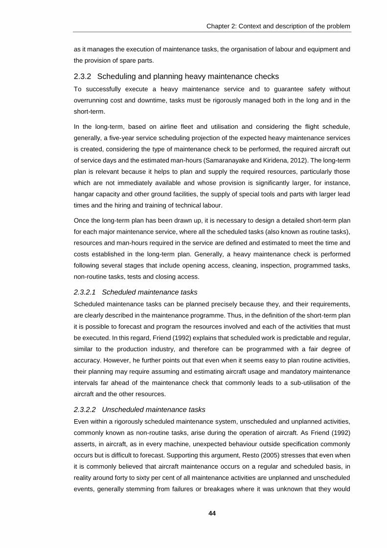
Chapter 2: Context and description of the problem
44
as it manages the execution of maintenance tasks, the organisation of labour and equipment and
the provision of spare parts.
2.3.2 Scheduling and planning heavy maintenance checks
To successfully execute a heavy maintenance service and to guarantee safety without
overrunning cost and downtime, tasks must be rigorously managed both in the long and in the
short-term.
In the long-term, based on airline fleet and utilisation and considering the flight schedule,
generally, a five-year service scheduling projection of the expected heavy maintenance services
is created, considering the type of maintenance check to be performed, the required aircraft out
of service days and the estimated man-hours (Samaranayake and Kiridena, 2012). The long-term
plan is relevant because it helps to plan and supply the required resources, particularly those
which are not immediately available and whose provision is significantly larger, for instance,
hangar capacity and other ground facilities, the supply of special tools and parts with larger lead
times and the hiring and training of technical labour.
Once the long-term plan has been drawn up, it is necessary to design a detailed short-term plan
for each major maintenance service, where all the scheduled tasks (also known as routine tasks),
resources and man-hours required in the service are defined and estimated to meet the time and
costs established in the long-term plan. Generally, a heavy maintenance check is performed
following several stages that include opening access, cleaning, inspection, programmed tasks,
non-routine tasks, tests and closing access.
2.3.2.1 Scheduled maintenance tasks
Scheduled maintenance tasks can be planned precisely because they, and their requirements,
are clearly described in the maintenance programme. Thus, in the definition of the short-term plan
it is possible to forecast and program the resources involved and each of the activities that must
be executed. In this regard, Friend (1992) explains that scheduled work is predictable and regular,
similar to the production industry, and therefore can be programmed with a fair degree of
accuracy. However, he further points out that even when it seems easy to plan routine activities,
their planning may require assuming and estimating aircraft usage and mandatory maintenance
intervals far ahead of the maintenance check that commonly leads to a sub-utilisation of the
aircraft and the other resources.
2.3.2.2 Unscheduled maintenance tasks
Even within a rigorously scheduled maintenance system, unscheduled and unplanned activities,
commonly known as non-routine tasks, arise during the operation of aircraft. As Friend (1992)
asserts, in aircraft, as in every machine, unexpected behaviour outside specification commonly
occurs but is difficult to forecast. Supporting this argument, Resto (2005) stresses that even when
it is commonly believed that aircraft maintenance occurs on a regular and scheduled basis, in
reality around forty to sixty per cent of all maintenance activities are unplanned and unscheduled
events, generally stemming from failures or breakages where it was unknown that they would

Chapter 2: Context and description of the problem
45
occur. In the same vein, Samaranayake and Kiridena (2012) remark that one half of the overall
maintenance workload within heavy maintenance originates from unplanned maintenance
activities arising out of inspections carried out during an aircraft lay-up.
Compared with routine tasks, non-routine activities can be more complex to plan, as they originate
from stochastic events, hence their requirements are not easy to foresee and, therefore, difficult
to forecast and program. Although the possible occurrence of unscheduled activities is considered
and roughly estimated in the initial plan, generally the necessary resources to accomplish them
are not immediately available. Thus, trying to prepare for all possible but uncertain non-routine
tasks would be inefficient and unaffordable.
Once an undetected failure or damage occurs, it usually increases over time and spreads,
producing more noticeable failure signs, leading to its detection and correction by programing a
non-routine task (Fard and Melachrinoudis, 1991). Non-routine activities usually originate in four
different ways. The first arises during the execution of scheduled inspections and checks after
maintenance personnel find damage and discrepancies that must be corrected. The second
source is aircraft logbooks, where pilots and cabin crew report abnormalities and malfunctions
during the flight. The third is failure analysis, where the non-routines are generated after finding
evidence of deterioration or damage during continuous monitoring and analysis of aircraft
systems. Finally, non-routine tasks are required to repair damage to aeroplanes caused by
external events such as hail damage, lightning strikes, bird strikes, hard landings, damage from
ground equipment handlers, etc. (Duffuaa and Andijani, 1999; Resto, 2005).
As illustrated in Figure 2-8, during heavy maintenance execution, mainly during the inspection
stage, unexpected damage, failures and discrepancies are discovered and need to be corrected
by programming additional unscheduled tasks. These non-routine tasks might require
programming supplementary activities and allocating additional resources, forcing adjustments
and changes to the initial maintenance plan, causing delays and disruptions within the whole
process.
Unscheduled maintenance is the most undesired event for any aircraft operator, as it tends to be
more costly than scheduled maintenance. Additionally, it has significant repercussions for the
spare parts supply chain and inventory management, resource planning and allocation, and
execution and control of maintenance. Furthermore, these unplanned activities can lead to delays
and cancellations and can have a significant impact on an aircraft's return time, cost and customer
service. Therefore, for airline operators and MROs, managing these activities becomes a crucial
aspect of the heavy maintenance process (Kumar, 1999; Resto, 2005; Al-Garni et al., 2009;
Papakostas et al., 2010; Samaranayake and Kiridena, 2012).

Chapter 2: Context and description of the problem
46
Figure 2-8 Delays and disruptions in the heavy maintenance process
Even when heavy maintenance services can be planned and scheduled by using experience and
statistical data and by taking advantage of informatics tools, there is a huge uncertainty caused
by the stochastic nature of unscheduled tasks. Nowadays, it is still common to see delays and
disruptions during major checks, so that operators and MROs are still searching for better ways
to predict non-scheduled tasks and reduce their negative effects over the scheduled plan.
Papakostas et al. (2010) and Samaranayake and Kiridena (2012) support this argument,
explaining that despite the progress accomplished in recent years through more sophisticated
Enterprise Resource Planning (ERP) software solutions and maintenance information and
decision support systems, these tools still have limitations and do not provide the necessary
support for scheduling and managing uncertain and complex unscheduled maintenance tasks.
2.3.3 Heavy maintenance challenges
Srinivasan et al. (2007) identify five main challenges that are commonly faced during the heavy
maintenance process. The first stems from the inherent complexity of aircraft major repair and
overhaul which arises from the large number of maintenance tasks to perform, especially those
due to unexpected and unpredictable damage that might require additional activities and
resources. The second challenge lies in the limited amount of resources (i.e. workforce, facilities,
tools and parts) available to perform the maintenance tasks, which may have a cascading effect
that occurs when problems in one service start affecting other aircraft checks that share
resources, similar to the problems described by Yaghootkar and Gil (2012). The third challenge
is the complexity of synchronising and managing the several resources required for each
maintenance task once the available resources are allocated. The fourth is the coordination and

Chapter 2: Context and description of the problem
47
agreement of objectives and priorities between departments in an uncertain and competitive
environment and the fifth arises from the execution, coordination and control of the myriad tasks
that must be executed according to the plan.
The complexity of heavy maintenance might cause delays and disruptions, which may lead to
serious operational, technical and economic consequences. Operationally, if the delay at the end
of the service is considerable, i.e. the duration of the heavy maintenance check is longer than
planned, it will alter flying schedules, delaying or, even worse, cancelling flights. Additionally, as
heavy maintenance services are programmed one after another, delays can affect subsequent
maintenance checks. If the problem is recurrent, it will cause a domino effect, affecting both short
and long-term maintenance plans. Delays in the heavy maintenance process may have an
economic impact for an airline by increasing costs or by reducing revenue. With regard to costs,
for example, the pressure to reduce delays forces management to increase available workforce
(hiring, boosting overtime or transferring personnel from other areas), and to purchase parts and
tools urgently (paying higher prices than regular ones). Regarding revenue, if an aircraft stays on
ground for longer than expected, it will affect the commercial itinerary and hence lower the number
of available seats, which ultimately leads to a reduction of income-earning capacity.
The main features and challenges of heavy maintenance in the aircraft industry are shared with
large and complex projects in other industries, such as construction. Both operate with high levels
of uncertainty and overrunning costs and lead times occur commonly. Both require a large
workforce and supplying and managing parts and materials is complicated. Masmoudi and Haït
(2012) argue that heavy maintenance can be understood as a multi-project with numerous
uncertainties, involving various but limited resources that must be shared either within the process
or externally (i.e. a project with high variability and high dependency). Williams (2003) describes
a complex project as a process in constant change during its execution, where several
interdependent internal and external factors interact, many different resources are involved and
uncertainty is present throughout the project.
2.4 Summary
This chapter aimed to support the empirical conception of the research by explaining and
describing the problem and its context, taking into account both personal experience in the
industry and the evidence provided by authors and experts in the field. The following paragraphs
recap the main ideas explained in this section.
The airline industry contributes significantly to globalisation. It enhances the connection of people
and goods, reduces transportation times, promotes tourism and facilitates trade and has a key
role in economic growth and social development worldwide. However, it is an industry operating
within a very competitive and dynamic market and is highly sensitive to external factors. It is
characterised by large revenues but low-profit margin levels. For this reason, airlines have been
forced to reduce costs and increase revenues without compromising service quality. Part of this
pressure has been transferred to the aircraft maintenance division due to its importance for
airlines.

Chapter 2: Context and description of the problem
48
The maintenance of an aircraft and its components is one of the main direct operating costs for
an airline. Moreover, it is a mandatory duty to ensure the safety of air operations. Maintenance,
therefore, must be carried out at the lowest possible cost but to the highest quality standards and
in compliance with a specified schedule. To accomplish these objectives, commercial aviation
maintenance is organised in a systematic and well-structured programme of scheduled tasks.
Notwithstanding the rigorous maintenance programme, during the execution of the maintenance
scheduled tasks unexpected damage and failures are commonly discovered. These must be
corrected by programming supplementary maintenance activities and allocating additional
resources to those originally planned. The changes in the original plan hinder the management
of the maintenance check, leading to interruptions during the process, delaying checks and
overrunning costs.
Aircraft heavy maintenance is a critical process, which requires the aircraft to be out of service for
a large period of time ranging from 7 to 30 or more days. Moreover, during its execution, a great
number of maintenance tasks are performed that require a considerable amount of resources in
constant interaction. Additionally, due to uncertainty related to unscheduled tasks, managing
heavy maintenance is complex and most of the time inexact.
Based on the evidence presented in this chapter, the problem can be summarised as follows:
a) There is a complex interaction between scheduled and unscheduled tasks and the large
amount of resources required to accomplish them.
b) Due to the stochastic nature of non-routine tasks, planning unscheduled activities and
forecasting their required resources represents an important challenge for maintenance
managers.
c) As a result of the previous points, adjusting an initial maintenance service plan and
managing a whole process can be tortuous and complicated and might impact upon lead
times, costs and even the quality of maintenance service.
In this chapter, the heavy maintenance process has been explained along with its relevance and
complexity, giving rise to the problem definition. Based on real facts and supported by different
studies, this chapter presented evidence to indicate that the described problem is real and
relevant in the airline industry and justifies the necessity of further research. Therefore, one of the
aims of the following chapter will be to perform a literature review to determine if the described
problem has been studied before and how this or similar problems have been approached and
analysed by other researchers.

49
Chapter 3: Literature review
Aircraft heavy maintenance has been shown to be a significant topic, not only due to the
operational, safety and financial impact for airlines and MROs, but because of the complexity and
uncertainty surrounding it. The heavy maintenance problem has been contextualised, explained
and justified in the previous chapter. However, it is necessary to explore how the stated or similar
problems have been addressed. Therefore, this chapter presents a comprehensive literature
review, firstly, to support this research by discussing the relevant theory related to the topic and,
secondly, to discover the different approaches used to study problems with high complexity and
uncertainty. This critical analysis attempts to determine the strengths and limitations of previous
studies and identify potential gaps where this study can contribute.
The chapter is structured as follows: firstly a review of the most commonly faced problems within
the aircraft maintenance field and the methodologies used to address them, secondly, a
description of the basic concepts and relevant works in project management due to the great
resemblance between heavy maintenance and complex projects and thirdly a revision of
uncertainty, one of the most important features of the problem, and some of the theories to explain
it. Finally, as an approach to understand complex systems, a review of simulation methodologies
was performed focusing on system dynamics and discrete event simulation.
3.1 Aircraft maintenance planning, scheduling and management
The main objective of this section is to review the literature of the aviation industry, mainly focused
on aircraft maintenance, serving two different purposes: firstly, to identify if the proposed research
problem has been studied or analysed before, and if so, how it was tackled, which methodologies
were used for addressing the issue, and what were the results obtained, and secondly to
determine different perspectives applied to study and tackle the most common problems in
aviation maintenance, which could be strongly related to the stated problem. As a result of this
examination, relevant and original studies were selected and analysed. In the following
paragraphs the studies are briefly described and organised into four categories: 1) researchers
interested in the planning and scheduling of maintenance, both in the long- and short-term; 2)
studies focused to tackle workforce problems; 3) works that analyse the management and supply
of materials and parts; and 4) those who propose alternatives to improve the maintenance
process.
3.1.1 Maintenance planning and scheduling
The airline scheduling process comprises four main parts: flight schedule preparation, fleet
assignment, aircraft routing, and disruption recovery. The flight schedule preparation considers
the list of flight legs along with departure and arrival times. The fleet assignment specifies which
aircraft types are going to operate a specific flight leg. In the aircraft routing, each aeroplane of
the fleet is assigned a specific route to operate. The disruption recovery reacts to all operational

Chapter 3: Literature review
50
disruptions by adjusting, updating and reassigning aircraft to new routes in order to minimise the
affectations (Stojković et al., 2002; Sarac et al., 2006; Papakostas et al., 2010; Reiners et al.,
2012).
The long-term maintenance plans are developed considering the first three categories and the
time intervals and durations defined in the aircraft maintenance programme. Short-term
maintenance scheduling considers the disruption recovery to adjust the maintenance activities
according to the daily operations, with strict compliance with the regulations (Papakostas et al.,
2010; Reiners et al., 2012).
With regard to heavy maintenance, two main elements comprise its programming: service
scheduling, and planning and scheduling of maintenance activities. Service scheduling considers
the overall scheduling of a fleet of aircraft at specific hangars taking into account the maintenance
services to accomplish, the itinerary, and the available facilities; it is also known as heavy
maintenance master plan. Meanwhile, planning and scheduling of maintenance activities refers
to the detailed plan of a specific maintenance service for a particular aeroplane, considering all
the maintenance tasks to execute, and the required materials, resources and workforce. In other
words, service scheduling refers to the long-term maintenance planning, while planning and
scheduling of maintenance activities is a short-term service based on the master plan
(Samaranayake and Kiridena, 2012).
In order to offer a quality service, the reliability and punctuality of flights are one of the main goals
of an airline, and maintenance must be aligned to this purpose. It is essential to minimize the
possibility of delays without affecting the safety and by keeping the costs in control. Therefore,
planning and scheduling of the maintenance activities, before and during the service is a widely
addressed research field.
3.1.1.1 Long-term planning
Long-term maintenance planning is used to determine and pre-allocate the resources required to
perform the maintenance activities. Long-term maintenance planning is done in conjunction with
aircraft routes and crew schedules, in order to consider operational, financial and regulatory
aspects. The analysed studies have paid attention to aircraft and components planning,
particularly components that are essential or critical.
Regarding aircraft planning, Warrington et al. (2002) designed an aircraft reliability and
maintenance model based on Discrete Event Simulation (DES), aiming to analyse the periods of
time in which the aircraft shall operate without failure or without the need of maintenance, also
known as the maintenance free operating period. The model helps to identify and differentiate the
essential, desirable and un-desirable maintenance activities. Another relevant study was
presented by Hahn and Newman (2008), which introduced a deployment and maintenance
schedule for a helicopter fleet, using mixed integer linear programming, as a proposal to reduce
scheduling times and avoid inconsistencies in the programme.

Chapter 3: Literature review
51
For critical aircraft components and parts limited by time, Fard and Melachrinoudis (1991)
developed a mathematical model to determine the best inspection schedule for aircraft critical
parts to minimize total maintenance costs. Their proposal is a stochastic optimization model with
a non-linear objective function and a single set of bounded constraints on integer decision
variables. It considers the relationship between different costs involved in the maintenance: cost
of inspections, cost of repairs and cost of catastrophic failures to determine the best balance
between them. Similarly, to determine which maintenance activities to perform and when,
Gustavsson et al. (2014) developed an integer linear programming model to schedule preventive
maintenance of the components of a system over a finite and discretized time horizon. The model
is dynamic to incorporate unexpected events, which are corrected by programming corrective
maintenance activities.
Particularly for engines and power plants, Bowman and Schmee (2001) proposed a model to
mitigate and manage financial risk for a MRO organisation. The model, based on DES, evaluates
the costs of long-term aircraft engine contracts to determine the fairest conditions for both parties
(airline and MRO). The model helps the organisation to take better decisions by analysing the
impact on costs and financial risk of operational and maintenance issues. Correspondingly,
Weckman et al. (2006) developed a decision support approach for modelling jet engine life and
estimating maintenance requirement for engine restorations. The model is based on real
statistical information, a hazard model and DES, aiming to predict the jet engine removal rate,
reducing additional spare engines and hence inventory costs.
3.1.1.2 Short-term scheduling
Sachon and Paté-Cornell (2000) suggest that for maintenance managers it is relevant to know
the impact of certain maintenance strategies both in aircraft security and flight delays to perform
an accurate decision. Therefore, they proposed a probabilistic risk analysis model, using influence
diagrams, to evaluate the effects of an airline's maintenance policy on delays, cancellations and
in-fight safety.
Some studies focus on the daily operation and maintenance of the aeroplane. For instance, Sarac
et al. (2006) explain that due to stochastic events, long-term plans are difficult to address and
hence they are often ignored by personnel in airline operations who are forced on a daily basis to
develop quick, ad hoc methods to address these eventualities. As an alternative, they proposed
an aircraft maintenance routing problem formulation considering maintenance resource
availability constraints. The proposal uses the branch-and-price algorithm to offer a short-term
planning solution (daily aircraft maintenance routing), incorporating resource availability
constraints into the model. In the same vein, Papakostas et al. (2010) explain that often during
line maintenance turn-around time (TAT) decisions regarding “go” or “no go” of the aeroplane for
the next flight must be taken, and that the time available to take that decision is limited and the
information available to analyse is considerable. They remark that currently that decision is taken
reactively resulting in high operational costs and low operational reliability. Therefore, they argue
that airlines need to create, simulate and evaluate different strategies of maintenance, reducing

Chapter 3: Literature review
52
unscheduled maintenance occurrences and some of their consequences. They introduced a
short-term planning model of aircraft line maintenance tasks during turn-around time at airports
stations, based on multi-criteria decision-making, allowing for immediate decision-making to
reduce or avoid reactive decisions. Similarly, Reiners et al. (2012) developed an algorithm
extending the traditional aircraft routing problem (ARP) by including profit and robustness, aiming
to mitigate the impact of unexpected events that hinder the management of the original flying
schedule. They used a network flow problem formulation and greedy start heuristics.
Another approach to analyse the daily operations is proposed by Tiassou et al. (2011) and
Tiassou et al. (2013). They developed a model to assess aircraft operational reliability with regard
to its missions in order to be able to cope with failures. They used a stochastic dependability
modelling approach to evaluate the capacity of the aircraft to keep operating for a specific time or
location without reaching an adverse status. If an unexpected event occurs while the aircraft is in
operation, the model assesses the ability to succeed in continuing on the remaining part of the
mission.
To cope with disruptions caused by unpredictable events, flight schedules need to be updated on
a daily basis, considering reassignment of aircraft, crew and passengers to reduce the effects as
much as possible. However, rescheduling issues can have a significant negative impact on costs
and service quality. Several works have analysed the recovery-rescheduling-rerouting problem of
flight operations.
Le et al. (2011) presented a literature review of current methodologies of airline recovery
optimization and airline disruption management of resources. They stress that in reality, the
itinerary and flights schedule does not operate as planned, as it is commonly disrupted by different
unexpected factors, such as maintenance problems or environmental conditions. They remark,
therefore, that it is necessary to find a minimal cost reassignment of aircraft and crews that
complies with all required safety rules, ensures the lowest impact on passengers and minimizes
operational difficulties for the airline. To tackle this problem, Stojković et al. (2002) developed an
optimization model to define new flight schedules based on planned crew transfers, rest periods,
passenger connections and maintenance, when minor perturbations occur. Their model is a dual
network based on PERT and CPM allowing both start times and activity durations as variables.
Similarly, Sriram and Haghani (2003) designed an optimization model for maintenance scheduling
and flight re-assignment to minimise costs. The model is formulated as a min-cost multi-
commodity network with integer constraints, using origin-destination schedule as input variables
and considering a heuristic approach. Meanwhile, Eggenberg et al. (2010) proposed a flexible
model to determine a recovery scheme, for each plane, crew member and passenger within a
certain makespan.
Another area of interest is the detailed programming of maintenance services. In this regard,
Kalton and Richards (2008) emphasise that the duration of a resource constrained project can be
two times or more larger than needed. They further argue that the approach used by most
commercial project planning software for handling resources, is a relatively inefficient

Chapter 3: Literature review
53
methodology for scheduling resource constrained projects. They performed a literature review
about the resource-constrained project scheduling problem, and compared the performance of
different scheduling engines, showing that engines can greatly impact upon the scheduling
programme results. Masmoudi and Haït (2012) designed a model for project scheduling and
planning problems, for modelling the periodic workload on a tactical level and the continuous
workload on the operational level, particularly for heavy maintenance services. They integrated
uncertainties into tactical and operational multi-resource, multi-project planning by using a fuzzy
and possibilistic approach instead of a traditional stochastic approach since limited data was
available. In their research, they identified different uncertainties during the aircraft heavy
maintenance process and classified them into different sources. By using the model, different
workload scenarios according to different time durations were proposed and assessed.
3.1.2 Workforce planning and scheduling
Workforce scheduling is a difficult task that involves personnel preferences, coverage constraints,
legal restrictions and many other constraints (Van den Bergh et al., 2013). Since the workforce in
aviation maintenance is highly skilled, specialized and costly, several studies have focused their
attention on addressing, analysing and attempting to solve workforce issues, mainly related to the
planning and scheduling of the maintenance labour. In this regard, different approaches have
been utilised to study manpower problems.
Latorella and Prabhu (2000) focused on human error in aircraft maintenance and inspection,
performing a literature review regarding relevant concepts and approaches for identifying,
reporting, and managing human error. They point out that aviation maintenance and inspection
tasks are commonly performed in an environment with time pressures, sparse feedback and
sometimes difficult ambient conditions, which, in combination with human erring tendencies,
result in varied forms of error which can impact upon safety, costs and quality.
Optimisation models have been commonly used for workforce scheduling. For example, Alfares
(1999) proposed an Integer Programming Model for scheduling workforce of an aircraft line
maintenance unit, motivated by high workload levels and by excessive overtime rates. The
objective of the model is to fulfil work requirements at minimum cost by determining the optimum
maintenance manpower schedule. Alfares’ model addresses an actual problem in aircraft
maintenance, showing real economic benefits from its implementation. However the model makes
some strong assumptions that are important to mention: for instance, the non-scheduled activities
were roughly estimated from a percentage derived from the routine task, even when this could be
inaccurate and unrealistic. Additionally, some human and organisational factors, such as unions
or performance decrease caused by fatigue, were not properly factored into the model. A similar
approach was used by Beliën et al. (2013). They proposed a model to minimize workforce costs
of aircraft line maintenance. The model uses an enumerative algorithm in a mixed integer linear
problem (MILP) to determine the number of personnel necessary to meet the maintenance
demand and to define the scheduling program that translates the availability of the staff into an
adequate shift structure. It is important to note that the model deals with scheduling and staffing

Chapter 3: Literature review
54
problems simultaneously and does not consider the possible effects of unscheduled maintenance
tasks. Meanwhile, Yang et al. (2003) and Yan et al. (2004) proposed a mathematical programming
model to offer a workforce supply plan, taking into account the technicians' maintenance
certificates and other related operational constraints. The model considers three different flexible
strategies: flexible shifts, flexible squad size and flexible working hours by applying mixed integer
programs. An important point to note in this research is that for the manpower planning, relevant
attributes of the technical personnel, such as their maintenance certificates and their technical
skills, were considered.
Another optimisation approach is proposed by Cheung et al. (2005). They suggest that it is
complicated to select and assign the most suitable person to perform skilled maintenance
activities. Moreover, they remark that scheduling and allocating personnel to ensure they can
meet the maintenance workload is a primarily a subjective process. Therefore, they developed a
decision support expert system for manpower allocation in aircraft maintenance services.
Analytical Hierarchy Process (AHP) was used for developing the model as it deals with
quantitative and qualitative criteria and sub-criteria, and combined with fuzzy logic to minimize
the weakness of AHP facing uncertainty. One of the strengths of the system is that it reduces
subjectivity on manpower and workload allocation by using quantitative and qualitative criteria.
Their results revealed that the system provides better workforce management and higher
productivity for the aircraft maintenance.
Quan et al. (2007) explain that aircraft maintenance managers face the dilemma of either
curtailing manpower to reduce idle time, or increasing it to improve maintenance productivity. To
tackle this dilemma, they developed a multiple objective problem (MOP) to optimise the heavy
maintenance process while reducing manpower costs. They applied utility theory to discover
Pareto optimal solutions and evolutionary algorithms to solve the multi-objective problem. This is
an original approach to optimise manpower, as it considers two different and opposite objectives.
However, some important variables in workforce management, as skills and certifications, are
overlooked.
Wagner and Fricke (2006) use a different method. They argue that workforce planning for both
scheduled and unscheduled maintenance is fundamental for avoiding expensive overcapacities.
They introduced a statistical model that represents the occurrence of failures as a stochastic
process to estimate the man-hour demand necessary to handle unscheduled maintenance events
on a certain fleet during line maintenance.
Another approach widely applied is the use of simulation models. Bazargan and McGrath (2003)
designed a model based on DES to analyse and improve aircraft availability and maintainability.
The research was motivated by poor maintenance planning causing higher rates of fleet
unavailability. Through building and comparing different what-if scenarios, they proposed a
workforce timetable re-schedule and the redistribution of technicians across different shifts,
reducing aircraft waiting time and increasing workforce utilisation. In a similar way, to tackle low
labour utilisation in line maintenance process, Gupta et al. (2003) developed a stochastic

Chapter 3: Literature review
55
simulation model for aircraft line maintenance to improve workforce allocation and increase labour
utilisation. Van den Bergh et al. (2013) also used simulation, combining DES and data
envelopment analysis (DEA) to design a model for managing aircraft line maintenance workforce
scheduling. The model first calculates different feasible low-cost rosters which are then evaluated
through the DES model. Finally, the most efficient alternatives are determined using DEA.
3.1.3 Management and supply of parts
In aircraft maintenance, large amounts of parts and materials are required. Additionally, they must
fulfil strict regulations to be approved and certified, hence becoming significantly expensive and
requiring large periods for supplying. For these reasons, the management and supply of parts
has been an area of great interest for several researchers.
For example, Ghobbar and Friend (2004) stress that implementing material requirement planning
(MRP) in the aviation industry could be complicated, as the aircraft maintenance process is
complex and full of uncertainties, thus the need for spare parts is unpredictable. They performed
a review in the industry using interviews to determine the most common inventory procedures
and policies used by airline operators and MROs, and to analyse the use of MRP for controlling
inventory, reducing stock and therefore costs. In the same vein, Cohen and Wille (2006)
investigated the effect that sharing part consumption data from heavy maintenance checks from
different MRO and airline operators has on the planning and procurement of parts. They found
that adopting a coordinated data-driven approach for managing parts might reduce the service
parts inventory and improve parts availability.
Kilpi and Vepsäläinen (2004) developed a statistical model to assess the effect of reducing the
inventory level through the implementation of an inventory pooling strategy, focusing on the spare
units needed to cover unscheduled removals. They concluded that inventory pooling of spare
components between airlines can significantly reduce inventory costs. Similarly, but focused on
aircraft engines, Joo and Min (2011) explain that engine modular design makes field maintenance
simple and agile, although it increases considerably the cost of the spare modules and inventory.
They remark that rigorous inventory control of spare modules is essential for cost-efficient
maintenance, and introduced a dynamic model for scheduling preventive maintenance of engine
modules. Their algorithm seeks to minimise the difference between due time for preventive
maintenance and actual time for preventive maintenance, considering that the spare modules to
support this type of maintenance are limited.
3.1.4 Process improvement
Aircraft maintenance is a complex process which requires a large amount of resources and
involves several activities. The inherent uncertainty that characterises this process makes it
challenging to manage. Moreover, due to its significant impact on costs and revenues for the
airline, there is constant pressure to improve the process. Different researchers have studied and
proposed new approaches to achieve this goal. Their proposals range from the use of
mathematical models and simulation or the application of information technologies to the adoption
of a continuous improvement philosophy.

Chapter 3: Literature review
56
Simulation has been widely used as a supporting tool for aircraft maintenance improvement.
Duffuaa and Andijani (1999) designed a framework for a simulation model that integrates
maintenance activities and operations. They advocate that in the airline industry it is essential to
treat maintenance and operations as one system, because of the high degree of dependency
between them. Meanwhile, Cobb (1995) proposed a simulation model in aircraft line maintenance
to reduce turnaround time, improve quality and reduce cost. Even though the model does not
consider the uncertainties of the maintenance process, it serves to test the effects of changes in
the maintenance process. The results are used to estimate operational capabilities.
Correspondingly, and focused on aircraft critical components, Adamides et al. (2004) used
system dynamics to analyse the long-term performance of aircraft engine maintenance, arguing
that life-cycle engine maintenance is a dynamic system influenced by engine reliability and
maintenance, operational requirements, and maintenance infrastructure. The model is used as a
decision making supporting tool to compare different maintenance scenarios, and also as a
learning tool to understand the drivers of successful and poor maintenance and operational
performance.
Another example of simulation is given by Horning et al. (2012), who developed an interesting
model based on DES to simulate flight operations of an aircraft fleet and the resulting preventive
and corrective maintenance of each aircraft, considering also its condition-based maintenance.
Through the assessment of different maintenance policies, the model helps to forecast and
evaluate the availability and flying rates for the fleet and for individual aircraft.
Mohaghegh et al. (2009) remark that despite the significant improvements to analyse and model
safety and risk assessment, there is a lack of organizational safety risk frameworks. Therefore,
they proposed a hybrid approach to model organizational safety risk, incorporating organizational
factors. The hybrid approach integrates System Dynamics (SD), Bayesian Belief Network (BBN),
Event Sequence Diagram (ESD), and Fault Tree (FT). Likewise, Ostrom and Wilhelmsen (2008)
developed a risk model in aviation maintenance to improve aeroplane reliability and safety by
using probabilistic risk assessment methodologies. They further suggest that structural damage
increases the risk of an accident, emphasising the relevance of analysing, detecting and
assessing vulnerabilities during the inspection process for risk reduction.
A different aspect worth studying is the approached by Jian and Hong-fu (2004) who stress that
determining and budgeting maintenance costs are difficult tasks, due to the uncertainty and
complexity that characterise the process. However, these are fundamental tasks for cost
efficiency improvement and consumption reduction. To overcome this problem, they designed a
maintenance cost-forecasting model based on the project-evaluating method and the cost-
estimating relationships (CERs) method.
Considering the available statistical data from operational and maintenance records, Al-Garni et
al. (2009) state that monitoring and analysing this information is a fundamental task for airlines
and MROs, to give a timely follow-up to the performance of the aircraft and its components, and
to evidence any possible failures. However, they add that this monitoring is commonly performed

Chapter 3: Literature review
57
using sophisticated and complex statistical and other analytical tools that might be difficult to
explain and understand for practitioners. Therefore, they proposed the use of graphical
techniques, using cumulative and mean cumulative function plots for extracting key management
information from field failures. In recent years the amount of information available has increased
dramatically and with it the complexity of its mining and analysis. In this regard, Wang et al. (2009)
explain that nowadays information systems are used in every aspect of maintenance support,
becoming effective tools to assist the decision making and support the execution of maintenance.
Thus, they proposed an evaluation framework to measure the effectiveness of the Aviation
Equipment Maintenance Support (AEMS) informationalization.
Ayeni et al. (2011), through a thorough and systematic review of the literature, evaluated the
perception, progress and implementation of “Lean” philosophy within the aviation maintenance
industry, particularly in MRO organisations. They concluded that it is feasible to apply “lean” in
the aviation industry; however, it is not sufficient to achieve all the objectives set by the
organization. Besides, they found that “lean” has been mainly applied as a waste reduction
methodology rather than as a process improvement philosophy. An important drawback pointed
out in this research is that some basic and common practices in “lean” are difficult to implement
in the aircraft maintenance sector due to the complexity and uncertainty to estimate accurately
the required resources. In a similar way, with a lean and continuous improvement approach, Ward
et al. (2010) proposed an integral model of the operational system to enhance efficiency and
customer satisfaction through improving aircraft maintenance processes without neglecting safety
and quality. The model is based on participatory action research and blocker resolution process
aiming to identify and eliminate those activities that hinder maintenance performance.
An additional way to improve the maintenance process is by enhancing its supporting processes.
For instance, Cheung et al. (2005) designed a model using genetic algorithms (GA) to maximize
ground support vehicles utilization and to enhance the logistics of aircraft maintenance activities
by providing a faster but reliable way of managing ground equipment.
Finally, focused on heavy maintenance, Srinivasan et al. (2007) remark that long lead times for
repairing and overhauling aircraft is a serious and common problem for MROs. Hence, they
implemented Critical Chain Method aiming to reduce turnaround time. Similarly, Samaranayake
and Kiridena (2012) argue that current approaches in aircraft heavy maintenance for planning
and scheduling have a limited capacity to deal with contingencies arising out of inspections. They
proposed a single integrated framework considering uncertainties and supported by unified data
structures.
3.1.4.1 Summary of aircraft maintenance studies
After reviewing and analysing the relevant literature concerning the common problems of the
aviation industry, some important findings emerge. Regarding the methodologies utilised to
address the planning, scheduling and management of aircraft maintenance, two main approaches
were used: mathematical optimisation models and simulation modelling. Optimisation was
principally adopted to minimise costs and turnaround time, or to maximise aircraft utilisation and
Chapter 3: Literature review
58
availability, by scheduling or managing different resources, like materials and parts, or workforce.
Meanwhile, different simulation approaches have been utilised as forecasting and scenario
building tools, to support the decision making and management thinking.
It is also worth noting the different processes analysed. The three main aircraft maintenance
areas, namely, line maintenance, heavy maintenance, and components maintenance, have been
studied to address their particular problems. The most addressed process has been line
maintenance, because of its direct impact upon and close relationship with daily operations. Many
researchers have analysed it from different perspectives and using several approaches, mainly
focused on short-term maintenance scheduling, particularly to analyse the recovery scheduling
problem. Optimisation models have been the most common approach for addressing these types
of problems.
Heavy maintenance has been studied from different angles due to the complexity and uncertainty
that characterises it. Some studies have considered heavy maintenance as a complex project
and have addressed it by using project management techniques such as CPM, PERT and CCM.
Others have proposed the use of continuous improvement tools, for instance, lean and six-sigma.
Another approach is the utilisation of MRP for supply management and production planning. The
application of simulation methodologies like discrete event simulation and system dynamics has
also been proposed. However, as stressed by Samaranayake and Kiridena (2012) most of the
studies in heavy maintenance have focused on the service scheduling problem, i.e. on the long-
term, disregarding the detailed planning and scheduling of maintenance tasks and their
corresponding resources.
The studies in component maintenance have concentrated on critical components, particularly
aircraft engines. The reason for this preference could be due to their significant impact on the
operation, their strict regulation, and their high costs. Studies have focused on optimising the
inventory, increase the "time on wing” and improving the maintenance process and supply,
amongst other factors.
Workforce is one of the most, if not the most, important resources for aircraft maintenance; it is
costly, highly skilled with a lengthy training and certification process. For this reason, workforce
planning and scheduling have attracted significant interest in the field. Nevertheless most of the
studies have focused primarily on line maintenance, aiming to reduce idle time and costs and at
the same time improve workforce productivity.
As discussed in chapter two, delays and disruptions during the heavy maintenance process are
relevant, real and actual problems in the aviation industry. However, few studies have addressed
these problems by analysing and assessing the impact of non-scheduled activities on the delays
and disruptions and how that might affect the heavy maintenance goals. Supporting this
argument, Samaranayake and Kiridena (2012) suggest that in heavy maintenance there is poor
integration between the planning of materials and resources, the scheduling and control of
maintenance tasks and the execution of maintenance activities. They also emphasise the
importance of dealing with uncertainty associated with heavy maintenance planning and

Chapter 3: Literature review
59
scheduling. Regarding uncertainties, Papakostas et al. (2010) further assert that nowadays, the
decision support process in aircraft maintenance is mainly reactive and focused on resolving
unscheduled maintenance activities.
Most of the solutions offered by the studies reviewed fail to consider a systemic understanding of
the problem and do not take into account the impact that each part has within the whole process
and the relationship between them. Some studies did not consider uncertainties, or made very
rigid assumptions about them. Due to the different fleet, a global optimisation approach is not the
best way to address heavy maintenance planning in a MRO (Masmoudi and Haït, 2012).
Moreover, traditional project management methodologies do not have the ability to unfold different
contingent scenarios to deal with the uncertainty associated with the unscheduled activities
(Samaranayake and Kiridena, 2012). Other approaches, like continuous improvement or IT
developments, require a deep cultural change in the organisation as well as in the philosophy of
thinking and its implementation requires a huge effort.
After describing the main characteristics of aircraft heavy maintenance and reviewing significant
approaches used to address the most frequent challenges of this process, a great similarity
between aircraft maintenance and complex projects management is evident. Therefore, it would
be fruitful to discuss relevant concepts in project management and learn how problems with
similar characteristics have been addressed by using this discipline.
3.2 Project management
Projects, from very ancient times, have been managed in very diverse forms. However, the
concept of project management as a discipline is relatively recent. Currently, projects are carried
out in a globalised and highly dynamic environment and in a constantly changing world,
characterised by large availability of information and extremely competitive markets. Project
managers face constant and continuous pressure to minimise costs and increase profits, whilst
also improving quality, efficiency, productivity and customer satisfaction. Project management
has evolved to support the achievement of project goals in a broad range of fields, mainly those
with high levels of complexity and uncertainty. Hence, before discussing relevant approaches for
analysing problems with similar characteristics to the research problem proposed, it is necessary
to explain the most significant concepts in the project management field.
Project management can be defined as the application of knowledge, skills, experience,
processes, methods, tools and techniques to achieve the project objectives (Project Management
Institute (PMI), 2013; Association for Project Management (APM), 2015b). In addition, according
to the British Standard BS 6079-2:2000, project management considers, the planning, monitoring
and control of a project and the motivation of the people involved, in order to achieve the project
objectives according to the specified time, cost, quality and performance (MS/2 British Standards
Institution, 2000). Furthermore, it is emphasised in the BS 6079-1:2010 that project management
is beneficial for an organization in different ways as it enables a more efficient use of resources
and has been shown to be an effective tool for managing many types of change (MS/2 British
Standards Institution, 2010).
Chapter 3: Literature review
60
3.2.1 Project
A project “is a temporary organization to which resources are assigned to do work to deliver
beneficial change” (Turner, 2009, p.2). Similarly, the PMI (2013) defines a project as a “temporary
endeavour undertaken to create a unique product, service, or result” (PMI, 2013, p.2). Projects
can also be seen as engines of change (MS/2 British Standards Institution, 2010). They have
distinct attributes that characterise and differentiate them from other routine work. The
combination of different factors, such as context, time frame and objective, make a project unique.
Additionally, they are finite, which means they have a well-defined starting and ending date. The
objective and expected results of a project are known and clearly stated at its definition. In order
to meet these objectives, different resources must be assigned. However, projects are always
subjected to several constraints, generally measured in terms of time, cost and quality.
Importantly, projects are rarely isolated as they have constant interaction with other projects and
external entities. Lastly, projects are usually carried out under risk and uncertainty conditions
(Williams, 2003; Buttrick, 2009; MS/2 British Standards Institution, 2010; PMI, 2013).
A project is not a static element: rather it is an entity in constant dynamism that evolves through
different stages to accomplish its objectives. These stages, or phases, are commonly known as
the project life-cycle and although different authors refer to them in different ways, in principle
they share a similar meaning. The PMI points out that the project phases’ names and numbers
are determined by the needs of the organisation involved in the project, the nature of the project
itself and its area of application. The PMI further adds that these steps are generally sequential
and time bound, with a specific start and ending point. Generally, a project is composed by the
following phases: 1) Appraisal, where the viability and feasibility of the project are assessed to
determine if it is possible or beneficial to carry out the project. 2) Design, where the concept of
the project is formalised by defining the plan of activities and by determining the resources, budget
and time required to perform the project. 3) Execution, where the activities are carried out and the
resource utilised. Rigorous monitoring must be performed during execution to ensure that the
project is run according to plan and to determine whether it is necessary to take corrective actions
to adjust it. Finally, 4) Close-out, which refers to the stage once the project has been completed,
where the project is formally finished, all relevant documentation is completed, the product or
service is delivered and the resources are released. Usually, a final evaluation and feedback is
performed to determine what went wrong and what went well (PMI, 2013).
It is important to highlight that in the final stage of the project life-cycle, a project is considered to
be completed when its objectives have been reached, but also it can be terminated because the
objectives cannot be met or if the project is no longer needed, or if the client asks to terminate it
(PMI, 2013).
3.2.2 Complex project
Complex project is a concept widely used in project management literature, yet it is commonly
applied as a synonym for large projects. Nevertheless, its definition is not as straightforward as it
might seem, and very few studies in the field have formally defined it.

Chapter 3: Literature review
61
Smith (2003b) explains that uncertainty is inherent in all projects, but he emphasises that the
higher the uncertainty level, the greater the complexity of the project. In the same vein, Meredith
and Mantel (2012) point out that in many complex projects, as a consequence of uncertainty, not
all activities are fully understood until some earlier activities have been completed. Complexity is
not just a question of the number of components or their relationship, but of numerous interactions
and the sophisticated connection between them. In other words, complexity represents the
interrelationship of components and how they act together within the project (Eve et al., 1997,
cited in Hetland, 2003).
According to Remington (2010), a complex project is one that shows a critical size, a very
constrained timeframe, a high level of ambiguity and a deep interconnectedness. Furthermore,
he argues that a complex project is indeed a complex adaptive system characterised by a nested
structure, a sophisticated communication network, both inside and outside, negative feedback
loops that induce stability, but also positive loops that encourage change, adaptiveness in
response to external stimulus in the environment, and extreme dependence on initial conditions.
Supporting this argument, Stacey (2011) points out the main principles of complex systems. He
suggests that due to the non-linear relationship of positive and negative feedbacks, unexpected
and counterintuitive results are normally produced by complex systems. Moreover, the sensitivity
to change is variable in complex systems, where the links between cause and effect could be
distant in time and space. A complex system can be more sensitive to some changes than to
others and uncertainty makes it difficult to determine which change will have the greater impact.
Williams (2003) argues that project complexity arises from two main dimensions: structural
complexity and uncertainty. The former is sub-divided into size, or number of elements, and
interdependence of elements, and the latter into uncertainty in goals and uncertainty in methods.
Size implies that the larger the number of elements in the project, and the larger the number of
activities to perform, the higher its complexity. Interdependence of elements suggests that the
large number of interrelations and the complicated interweaving of elements also increases the
complexity in the project. As a result of these two dimensions, structural complexity leads to a
complex system in which the whole is more than the sum of the parts. Complexity in goals arises
because there is vagueness or ambiguity in the project’s objectives, or because the objectives
are continually changing with the clients' requirements. Uncertainty in methods occurs when
methodologies or steps to perform are imprecise, unclear or unknown, causing continuous
changes in the plan and project structure. The two types of uncertainty generate perturbations in
the system, which result in complex, dynamic behaviour.
Interestingly, though using different concepts, Remington (2010) adopts a similar perspective
regarding complexity, suggesting that there are four types of complexity in projects, namely,
structural, technical, directional and temporal. Structural complexity is generally found in large
projects and it arises due to difficulty in managing and controlling the great number of
interconnected tasks and activities. Projects developing new products or services, or applying a
new technique or methodology without precedents experience Technical Complexity,

Chapter 3: Literature review
62
characterised by technical or design problems caused by the interconnection between multiple
interdependent solution options. Directional Complexity is the result of conflict or ambiguity in the
interpretation of goals and objectives, and is exhibited by projects with multiple and unshared
goals or divergent and unclear goal paths. Finally, Temporal Complexity is present in projects
carried out in highly unstable and dynamic conditions generally outside the control of the project
team. It arises from uncertainty regarding future constraints, unsteady environment or even
concerns about the survival of the system.
In summary, as already discussed, and supported by Latorella and Prabhu (2000), Ward et al.
(2010) and Masmoudi and Haït (2012), aircraft heavy maintenance is a highly dynamic and
intricate process, where uncertainty is present during execution. It involves several constrained
resources that interact both internally and externally and so fulfils the above definition of a
complex project. It can, therefore, be studied from this perspective. Moreover, the uncertainty,
complexity, and uniqueness of project activities make control more difficult and deviation from
plans more probable, because plans are formulated for a set of contingencies that cannot be
preconceived because they have no precedent (Sydow and Staber, 2002).
3.2.3 Risk
Risk is associated with project management and this association is particularly true for complex
projects. Smith (2003b) explains that “risk” comes from the Latin root “risicare”, which means “to
dare”, emphasising that from this etymological meaning, risk represents more a choice rather than
fate. According to Buttrick (2009), risk represents any potential uncertainty, threat or occurrence
that may affect the achievement, objectives and benefits of the project. Smith (2002), however,
argues that risk can bring opportunities as well as threats. It does not, therefore, necessarily have
negative consequences and can have positive ones.
Some relevant definitions of risk in the context of project management are the following:
In the BS 6079-2 2000, risk is defined as the “combination of the probability or frequency of
occurrence of a defined threat or opportunity and the magnitude of the consequences of the
occurrence” (MS/2 British Standards Institution, 2000, p.11).
According to the HM Treasury, risk is the “uncertainty of outcome, whether positive opportunity
or negative threat, of actions and events. The risk has to be assessed in respect of the
combination of the likelihood of something happening, and the impact which arises if it does
actually happen” (HM Treasury, 2004, p.9).
The Project Management Institute defines risk as “an uncertain event or condition that, if it occurs,
has a positive or negative effect on one or more project objectives such as scope, schedule, cost,
and quality” (PMI, 2009, p.310).
From these definitions, two relevant elements can be identified: uncertainty and consequences
or impact. Uncertainty refers to unexpected or unforeseen events that might happen either just
before or during the project execution. Uncertainty is generally described as a "probability",
"possibility" or "likelihood" of an unexpected event occurring. Sometimes, there is enough

Chapter 3: Literature review
63
information or knowledge to estimate the uncertainty using a probability distribution, but in others
it is based on perceptions and subjective judgments. If an unexpected event occurs, the
consequences may be positive or negative and so can be seen either as opportunities or threats.
This might influence the performance and objectives of the project.
3.2.4 Risk management
According to the Association for Project Management (2015a), risk management is the “process
that allows individual risk events and overall risk to be understood and managed proactively,
optimising success by minimising threats and maximising opportunities”. The Project
Management Institute (PMI) (2009) explains that project management addresses the uncertainty
in project estimates and assumptions by assessing and analysing the potential unexpected
events and conditions that might occur before or during the project. The PMI further indicates that
for successful project management, project risk management is neither an optional activity nor a
substitute for other project management processes and must, therefore, be considered in all
project phases.
The opinions of authors differ regarding the steps that comprise the project risk management
process. For instance, in the context of construction projects, Perry and Hayes (1985), Smith
(2003a) and Wood and Elis (2003) identify a three-step process for risk management, namely,
identification, analysis and response of risk. The Risk Analysis and Management of Projects
approach (RAMP) considers six separate stages known as opportunity identification, appraisal,
investment planning, asset creation, operation and close-down (Institution of Civil Engineers and
the Faculty and Institute of Actuaries, 2002). Meanwhile, the Project Management Institute (PMI)
(2009, 2013) defines six main steps in the risk management process: risk management plan, risk
identification, qualitative risk analysis, quantitative risk analysis, risk responses plan and risk
control. (Lester, 2014) proposes 5 stages for risk management: awareness, identification,
assessment, evaluation and management of risk.
All these classifications have remarkable similarities despite the different stages proposed.
Considering them all, it can be suggested that project risk management should consider: 1) Clear
definition of risk management objectives, process and scope. 2) Identification and categorisation
of potential risks that might influence performance and objectives, including documentation of
their main features. 3) A qualitative assessment to analyse the two elements of risk: uncertainty
and impact, in order to prioritise the different risks. 4) A quantitative analysis that involves the
application of a variety of numerical tools to assess the effect of the identified risks on project
performance. 5) Action plans to take advantage of opportunities and to minimise the effect of
threats. 6) The implementation of control and the adjustment of the proposed action plans to
ensure their effectiveness.
Smith et al. (2006) remark that risk management does not mean predicting the future: rather, it
means understanding the project to make better decisions regarding its management. Finally, it
can be summarised that risk management is a process to systematically identify, assess, analyse,

Chapter 3: Literature review
64
understand and manage uncertainties and their corresponding consequences. Therefore, it
becomes an essential part of project management to ensure the success of the project.
3.2.5 Relevant approaches in project management
Different approaches have been used to analyse a wide range of problems in project management
and this section summarises those considered as outstanding due to the close relation to the
problem subject of this research. For instance, in risk management, Chan and Kumaraswamy
(1997), Charoenngam and Yeh (1999) and Sambasivan and Soon (2007) identified and evaluated
the typical risk factors that cause delays in construction projects. (Bowers, 1994) proposed a
framework to determine, customise and combine uncertainty estimates based on quantitative and
qualitative data to determine the project uncertainty rating. Lee (2005) developed a simulation
model to determine the probability of completing a project in the specified time, considering the
randomness and stochastic nature of the activities’ duration. Schatteman et al. (2008) proposed
a heuristic methodology for determining and evaluating major risk factors, their probability of
occurrence and their impact on project duration, to define a robust project plan that can cope with
disruptions.
Regarding resource management, several methods have been applied. Dynamic programming
was used by Elmaghraby (1993) to minimise the project completion time considering the relation
between the resources allocated and the activity duration. Hapke et al. (1994) focused on
software development and developed a fuzzy project scheduling system to allocate personnel
between dependent activities under uncertain activity duration. Fatemi Ghomi and Ashjari (2002)
used a simulation approach to improve the utilisation of common resources during the execution
of concurrent projects. Genetic algorithms have been commonly used for resource planning and
allocation (Hegazy, 1999; Chang et al., 2001; Valls et al., 2009; Yannibelli and Amandi, 2011).
Other optimisation techniques have been also applied to the management of resources. Leus and
Herroelen (2004) used a branch-and- bound algorithm to develop a resource allocation model for
projects with variable activity duration. Brucker et al. (2011) suggested that workforce scheduling
problems can be formulated as integer linear programs and that the assignation of shifts to
personnel and the allocation of workforce to specific activities can be solved by applying network-
flow algorithms.
Several approaches to the planning and scheduling of activities in project management have been
utilised to support traditional techniques and mitigate their drawbacks. Herroelen and Leus (2005)
point out that the fundamental approaches for scheduling under uncertainty are reactive
scheduling, stochastic project scheduling, fuzzy project scheduling, robust (proactive) scheduling
and sensitivity analysis.
Fuzzy concepts have been widely used as a different way to represent and analyse uncertainty
in projects execution. Leu et al. (2001) used fuzzy set theory in combination with genetic
algorithms for a multi objective time-cost trade off under different risk levels. Özdamar and Alanya
(2001) used fuzzy numbers to represent the uncertainties related to activity durations and the
interrelation between them and applied them in conjunction with a generic heuristic algorithm to

Chapter 3: Literature review
65
planning software development projects. Oliveros and Fayek (2005) proposed a fuzzy logic model
for monitoring and controlling construction projects. Li and Chen (2007) and Long and Ohsato
(2008) used fuzzy sets to support a critical chain method for estimating the buffer size. Castro-
Lacouture et al. (2009) developed different fuzzy mathematical models for the multi-objective
optimisation of project schedules taking into account time, cost, and unexpected materials.
Zammori et al. (2009) used fuzzy logic and multi criteria decision analysis (MCDA) to support
critical path method (CPM) considering the critical parameters of the project.
Optimisation models have been widely used to study planning and scheduling problems.
Golenko-Ginzburg and Gonik (1997, 1998) utilised a zero-one integer programming problem for
the former and a heuristic approach for minimising the project duration for the latter. Fleszar and
Hindi (2004) used a variable neighbourhood search to reduce the solution search to address the
resource-constrained project scheduling problem. Zhu et al. (2004) developed a recovery plan to
get back on track as soon as possible at minimum cost using integer linear programming. Budai
et al. (2005) used a NP-hard mathematical formulation and a heuristic approach to minimise out
of service and maintenance costs for a preventive maintenance scheduling programme. Rabbani
et al. (2007) proposed a heuristic algorithm by combining CCM concepts and resource-
constrained project scheduling methods, aiming to minimise expected project duration and its
variance.
Simulation techniques and computer-based systems have been also used for planning and
scheduling. Lu and AbouRizk (2000) and Zhang et al. (2002) applied discrete event simulation
(DES) to improve CPM and PERT methodologies. Cho and Eppinger (2005) developed a
simulation model based on the design structure matrix (DSM) to identify leverage points for
process improvements and to evaluate alternative planning and execution strategies. Hegazy and
Menesi (2010) used the main concepts of the critical path method (CPM) to develop the critical
path segments (CPS) model that breaks down the duration of each activity into separate time
segments to avoid complex network relationships and facilitate resource allocation. Bruni et al.
(2011) designed a computer-supported system for making a robust project plan less sensitive to
unexpected events by considering the available probabilities to assess the project reliability and
minimise the impact of possible disruptions during project execution.
Other approaches use MCDA to support decision making by evaluating the importance and
criticality of certain activities (Mota et al., 2009) or to evaluate the project performance according
to different indicators considering the point of view of different stakeholders (Marques et al., 2011).
Bayesian networks have also been used to estimate delays in maintenance projects (Demelo and
Sanchez, 2008).
Several approaches have been proposed to support the traditional methodologies of project
management, e.g. CPM, PERT and CCM, especially to deal with complex projects and high levels
of uncertainty. Most of the proposals focus on mathematical optimisation models and computer-
aided simulation models. Their applications range from an operative and tactical level, to define

Chapter 3: Literature review
66
comprehensive project schedules as well as detailed resource allocation, to a strategic level as a
decision support tool for project managers to monitor the project status and test different policies.
3.3 Uncertainty
Uncertainty is an important concept for this research. In aircraft maintenance, uncertainty is
mainly caused by the potential occurrence of unexpected damage and failures that must be
corrected by programming unscheduled maintenance activities, which might require additional
resources and tasks, complicating the planning, scheduling and execution of the maintenance
service.
Uncertainty is commonly used in a variety of fields, including project management, to express
complexity and the unknown. However the concept of uncertainty might be misunderstood and is
sometimes confused with the concept of risk. Therefore, it is important to establish a formal
definition of uncertainty and discuss different arguments about it.
Chapman and Ward (2002, 2003) define uncertainty as a lack of certainty involving variability,
ambiguity and deficiency or absence of data, information, knowledge and understanding.
Meredith and Mantel (2012) explain that uncertainty refers to having partial or no information
about the situation or outcomes, often due to ambiguity or complexity. A broader definition is
offered by Klir and Wierman (1999), who specify that uncertainty represents the degree of
information deficiency, indicating how incomplete, imprecise, fragmentary, not fully reliable,
vague, contradictory or deficient the information available is.
Uncertainty is inherent to many aspects of life and Klir and Wierman (1999) suggest that
uncertainty cannot be avoided when dealing with real-world problems, being present at the
empirical, cognitive and social level, resulting in errors, misunderstandings, vagueness, ambiguity
and unavailability. Moreover, uncertainty is always present at a certain level in decision making,
and although it can be understood, managed, and even reduced, it cannot be eliminated (Belton
and Stewart, 2002). In the same vein, Smith (2003b) explains that in real world projects there is
always a certain degree of uncertainty, as it is extremely difficult to predict and control all events
relating to major projects.
Risk and uncertainty are used indistinctly as synonyms in daily life. However, it is important to
point out the differences between them. According to Knight (1921), the practical difference
between risk and uncertainty is that in the former the distribution of the outcome is known, while
in the latter it is unknown because the situation being addressed is unique. In a similar way, Pidd
(2004a) explains that risk and uncertainty are used to discriminate between options. He further
highlights that a decision concerning risk is one where, although it is not known precisely what is
going to happen, enough information exists to estimate a probability distribution of the outcomes.
In contrast, a decision concerning uncertainty relates to unique or uncommon situations where
there is no objective way to build the probability distribution and the outcome, therefore, is
unknown and must be estimated by different means. Williams (2003) uses a different terminology,
but also differentiates between these two concepts, arguing that there are aleatoric and epistemic

Chapter 3: Literature review
67
uncertainties, the first resulting from stochastic events and the second from lack of knowledge.
Importantly, he highlights that the latter increases the complexity of a project, hindering its
management.
Chapman and Ward (2002) explain the relation between uncertainty and risk from a different
perspective, stating that risk is a consequence or implication of an uncertain event or
phenomenon. They further point out that these unexpected consequences may be wanted
(positive) or unwanted (negative). Uncertain events and their implications must, therefore, be
understood properly in order to manage them successfully. Uncertainty and risk have the same
relationship in the context of project management. Smith (2003b) remarks that risk is a
consequence of uncertainty; it is generally interpreted as factors which might impact upon the
achievement of project objectives. According to the Project Management Institute (PMI) (2013),
project risk is an uncertain event that, when it occurs, has a positive or a negative influence on a
project’s objectives. From these points of view, it can be argued that risk involves the uncertainty
of an event, but also its consequences.
3.3.1 Classification of uncertainty
Uncertainty has been classified in different ways using different perspectives for particular
contexts. This gives a better understanding for analysis and management. These different
classifications, however, implicitly share some relevant concepts.
In terms of multi-criteria decision making, Belton and Stewart (2002) suggest that internal and
external uncertainty can be differentiated. They explain that internal uncertainty comprises two
aspects: the structure of the model and the judgmental inputs of the model. The first focuses on
problem structuring and model building and mainly relates to ambiguity and ignorance. The
second considers the elicitation of information and the utilisation of the model and mainly relates
to imprecision. They describe external uncertainty as a lack of knowledge about the
consequences of a particular choice, subdividing it in two groups: uncertainty about related
decision areas and uncertainty about the environment. The former refers to the influence that
some decisions can have on other interconnected decisions and the insecurity this can cause.
The latter denotes the concern about problems outside the control of the decision maker,
representing lack of knowledge or understanding and randomness.
In a project management context, Hetland (2003) identifies four different categories of uncertainty,
based on the crossed-relation between the availability of the information (how much is known)
and whether a project is closed or open. In a closed project, it is well defined what to do and how
to do it, whereas in an open project this is not the case. Therefore, the first type of uncertainty,
where there is full knowledge about the possible outcomes and the project is closed, is called
deterministic uncertainty; hence it is just a question of calculating the probability of occurrence of
each outcome. The second category is known as lack of information and also occurs in a closed
project. However, in this type of uncertainty, there are missing pieces of information that might
result in an incomplete or ambiguous understanding of the project and the challenge is how to
estimate the outcome using the incomplete available data. The third category is called variability

Chapter 3: Literature review
68
and occurs in an open project when the information is available. This approach differs from the
deterministic uncertainty because in this case the number of outcomes, their values and their
probabilities of occurrence are assigned subjectively based on the judgement or intuition of
experts supported by historical facts. The last category is known as undetermined uncertainty and
refers to an absence of information in an open project. It generally occurs in unique and highly
specialised projects where there is not enough information available. This type of uncertainty
represents the highest degree of complexity.
From the information analysis and management point of view, Klir and Wierman (1999) identify
three different types of uncertainty: fuzziness, strife or conflict and non-specificity, clarifying that
the last two are commonly grouped and recognised in a wider category known as ambiguity, as
shown in Figure 3-1. Fuzziness refers to the uncertainty that arises from the vagueness of
linguistic expressions or from a lack of clear or sharp definition. Strife is the uncertainty that results
from conflict or incongruence between different pieces of evidence regarding a set of alternatives.
Non-specificity is the type of uncertainty that occurs when some alternatives are left unspecified
or there is imprecision in characterising the different alternatives. Therefore, ambiguity expresses
the difficulty in determining or characterising a set of alternatives, either by discrepancy or
imprecision.
Figure 3-1 Basic uncertainty types (Klir and Wierman, 1999, p.103)
In aircraft maintenance, Masmoudi and Haït (2012) identify six different types of uncertainty and
classify them at the tactical and operational level. At the tactical level, they define three types of
uncertainty. Firstly, uncertainty in the release date where the days that the aircraft is going to stay
out of service are not precisely known and must be estimated. Secondly, uncertainty in the
workload where despite the scheduled tasks being known in advance, the programming of
unscheduled tasks hinders the planning of the workload. Finally, uncertainty in procurement
delays, where unplanned maintenance might require parts and material not included in the original
supply plan and affects procurement significantly. At the operational level, they also define three
Uncertainty
Fuzziness Ambiguity
Strife Non-specificity
Lack of definition or sharp distinction
Vagueness
Cloudiness
Haziness
Unclearness
Indistinctness
Sharplessness
Dissonance
Incongruence
Discrepancy
Conflict
Discord
Variety
Generality
Diversity
Equivocation
Imprecision
Disagreement in choosing amongst several alternatives
Two or more alternatives are left
unspecified
One to many relationships

Chapter 3: Literature review
69
types of uncertainty. Firstly, unexpected lack of resources (principally the absence of personnel)
which might affect planned daily progress. Secondly, task duration: in aviation maintenance it is
difficult to set a standard time for each activity, as it depends on different factors, e.g. the skill
level of the personnel, the condition of the aircraft, external conditions, etc. Finally, updates in the
maintenance program: sometimes manufacturers, authorities or operators require adjustments to
the maintenance plan by including, modifying or eliminating maintenance tasks. Masmoudi and
Haït (2012) further argue that the problem of tactical planning under uncertainty for aircraft
maintenance had never been studied until their proposed study.
3.4 Alternative uncertainty theories
Traditionally, and for more than three hundred years, uncertainty has been described and studied
using probability theory. However, uncertainty is a multidimensional concept formed from distinct
types of uncertainty and, in its simplest form, probability theory focuses on only one of these
dimensions (Klir and Wierman, 1999). During the second half of the 20th century, other notable
theories emerged that aimed to characterise the different aspects of uncertainty, namely, fuzzy
set theory, evidence theory and possibility theory (Klir and Wierman, 1999; Klir, 2003; Rogova
and Nimier, 2004; Maskell, 2008). Each particular uncertainty theory describes different forms of
uncertainty (predictive, prescriptive, diagnostic, etc.) in terms of a certain type of monotonic
measure (or a pair of measures) by using a specific formalised language system (Klir, 2003).
3.4.1 Fuzzy set theory
Fuzzy set theory was proposed by Zadeh (1965) for modelling uncertainty associated with
vagueness, imprecision and lack of information about the system, providing a “mathematical way
to represent vagueness in humanistic systems” (Özdamar and Alanya, 2001, p.159). A fuzzy set
“is a class of objects with a continuum of grades of membership. Such a set is characterized by
a membership function which assigns to each object a grade of membership ranging between
zero and one” (Zadeh, 1965, p.338). A relevant characteristic of fuzzy sets is their capability to
represent gradual transitions from membership to non-membership, which is important in
describing the vagueness and imprecision of expressions in natural language (Klir, 2001). Fuzzy
set theory is a generalisation of classical set theory, which represents a particular case when the
membership of an element can be defined unambiguously, i.e. where it is clear if the element
does or does not belong to the set.
3.4.2 Evidence theory
Evidence theory, also known as Dempster-Shafer theory, was proposed by Dempster (1967;
1968) and further formalised by Shafer (1976). It consists of two dual semi-continuous non-
additive measures called belief and plausibility measures. (Klir and Wierman, 1999). In the
Dempster-Shafer theory, an outcome of a random experiment is known as a proposition. The set
of all possible, mutually exclusive and collectively exhaustive propositions is called the frame of
discernment and the set of all subsets of the frame of discernment is known as the power set. A
basic probability mass can then be assigned to the subsets that form the power set (Yang and
Xu, 2013). Therefore, the belief measure of a particular preposition describes all basic probability

Chapter 3: Literature review
70
masses assigned exactly to that preposition and its smaller subsets, whereas the plausibility
measure of a specific preposition represents all possible basic probability masses that could be
assigned to the preposition and its smaller subsets. The belief and the plausibility measures can,
therefore, be interpreted as the lower and upper bounds of probability to which a certain
preposition is supported. The difference between the belief and plausibility measures of a given
preposition defines the degree of ignorance for that preposition (Yager, 1987; Dubois and Prade,
1991; Tonon, 2004; Yang and Xu, 2013). In contrast to classical probability theory, where
probability masses are only assigned to singleton subsets, in evidence theory probability masses
can be assigned to all subsets of the frame of discernment (Borotschnig et al., 1999).
The core of Dempster-Shafer theory is Dempster’s rule, which constitutes a conjunctive
probabilistic inference process to combine independent evidence that is fully reliable. However,
Dempster’s rule cannot be applied when two pieces of evidence support different propositions
and this lack of definition has led to a counter-intuitive problem when the rule is used to combine
evidence in high (or near complete) conflict (Zadeh, 1984; Zadeh, 1986; Haenni, 2005; Yang and
Xu, 2013).
Different evidence combination rules have been developed to overcome problems associated
with the non-definition and counter-intuitive problem associated with Dempster’s rule (Yang and
Xu, 2013). Yager’s rule (Yager, 1987) suggests allocating conflicting beliefs to the frame of
discernment. Dubois and Prade’s rule (Dubois and Prade, 1988) proposes the allocation of
conflict beliefs locally between focal propositions where the conflict occurs. Proportional Conflict
Redistribution 5 (PCR5) rule (Smarandache and Dezert, 2005) also proposes allocating conflicts
locally. However, in their attempt to deal with conflict, these rules have lost their probabilistic
nature, as they no longer constitute a conjunctive or probabilistic reasoning process (Yang and
Xu, 2013).
3.4.2.1 Evidential Reasoning (ER) rule
A new rule for evidence combination has been recently proposed by Yang and Xu (2013). This
new evidential reasoning rule allows multiple pieces of independent evidence to be combined
conjunctively and in any order. An important feature of the ER rule is that it considers the weight,
or importance, and the reliability or quality, of each piece of evidence. It constitutes a generic
conjunctive probabilistic reasoning process or a generalised Bayesian inference process (Yang
and Xu, 2014). The ER rule consists of two main elements: the bounded sum of their individual
support and the orthogonal sum of their collective support. Through a new reliability perturbation
analysis, the ER Rule overcomes the non-definition and counterintuitive problems associated with
Dempster’s Rule (Yang and Xu, 2013).
Yang and Xu (2013) demonstrated that Dempster’s rule is a special case of the ER rule when all
pieces of evidence are fully reliable. They also prove that the ER algorithm is a special case of
the ER rule, when reliability and weight are the same in all pieces of evidence and the latter is
normalised.

Chapter 3: Literature review
71
3.4.3 Possibility theory
Possibility theory was proposed by Zadeh (1978) and further investigated by Dubois and Prade
(1988, 1994) to handle certain types of uncertainty. Similarly to evidence theory, it uses two dual
semi-continuous fuzzy measures to deal with incomplete information or partial ignorance:
possibility, or lower semi-continuous, and necessity, or upper semi-continuous, both measures
are commonly understood as functions of the power set of a given possible set of prepositions
(Klir, 2003; Masmoudi and Haït, 2012; Borotschnig et al., 1999). Possibility theory is a natural
mathematical framework for describing and analysing uncertainty associated with fuzzy
propositions, where possibility and necessity are a special case of plausibility and belief measures
respectively and whose focal elements are nested. It represents a specific branch of evidence
theory (Klir and Wierman, 1999; Klir, 2003). In general terms, instead of providing a single value
like probability theory, possibility theory provides a “minimum possible value” and a “maximum
necessary value”.
3.5 Simulation
Since the development of computers, computer-based simulation has become a useful tool for
analysing complex systems and for decision support. Swain (1993) argues that simulation can be
useful for studying and analysing how a system reacts to changes in flow patterns or for obtaining
statistical estimates of important performance variables. Pidd (2004a) describes three common
approaches to analyse particular problems in management science: experiment directly on the
real system, construct and apply a mathematical model, or simulate the system. He further adds
that simulation can have significant advantages over the other two approaches. For example,
compared with direct experimentation, simulation can be cheaper, faster, safer and easier than
experimenting or practising in the real system. Compared with traditional mathematical modelling,
simulation can cope with dynamic effects. Robinson (2004) also explains the importance of
simulation, stating that it helps to deal with variability, interconnectedness and complexity, three
common characteristics of operations systems.
Due to its flexible capabilities, simulation has recently gained popularity for studying relevant
problems in the airline industry. Regarding aircraft maintenance, Cobb (1995) remarks that
simulation can support airlines and MROs for analysing and assessing long-term strategic
changes and short-term operational and tactical changes. Bazargan and McGrath (2003) argue
that simulation of maintenance activities can be a superior technique compared with traditional
analytical approaches. Supporting this argument, Gupta et al. (2003) explain that aircraft
maintenance is plagued by planning difficulties mainly caused by unpredictable failures and they
argue that stochastic simulation in particular presents relevant advantages over mathematical
modelling to study situations where randomness is present. Duffuaa and Andijani (1999) point out
three key features of maintenance that make simulation the most viable approach: complex
interactions between maintenance and other organization functions, the close interrelationship
between the elements involved in maintenance and the constant uncertainty that characterises
maintenance.

Chapter 3: Literature review
72
Simulation can be understood as the imitation of the operation of a real-world process or system
over time (commonly designing and using mathematical or logical models computer-based), to
describe, explain and predict the behaviour of the real process/system (Hoover and Perry, 1989;
Banks et al., 2000). Likewise, Madachy (2008) defines simulation as the numerical evaluation of
a model to describe and analyse a particular system, experimenting with given inputs to see how
the system performs; he further points out that simulation is used to explain system behaviour,
improve existing systems, or to design new complex systems. Law and Kelton (2000) distinguish
between static and dynamic simulation, where the former imitates a system at a point in time and
the latter imitates a system as it changes through time. Correspondingly, Robinson (2004)
describes dynamic simulation as (computer-aided) experimentation with a simplified and limited
version of an operations system as it changes through time, aiming to better understand and
improve the real system. Rotaru et al. (2014) state that the simulation of a system comprises
building a valid model to replicate the parts of interest of that system, then using the model and
experimenting within it to explore and understand the system’s functioning and performance
under certain conditions and in response to certain courses of action, with the aim of providing
scientific support for management thinking and decision support for process systems.
Pidd (2004a) explains that computer simulation is the utilisation of computer-aided models to
analyse and experiment through processing and analysing inputs to explore the effects or outputs
they might have in the real system. However, he indicates that any simulation approach is limited
and influenced by certain assumptions and considerations based on the particular perception of
reality. How the model (and the simulation) is developed and expressed depends on the specific
“worldview”.
It can be summarised that simulation is the act of using or “playing” with the models with the aim
of learning from them. Simulation allows experimentation with the model and specific input
variables in a controlled and safe environment to understand and analyse how the model, and
therefore the real system that it emulates, behaves. It also allows comparison between different
input variables to determine which perform the best.
The close relationship between real systems (or worldview) and their models and the learning
cycle are clearly explained by Sterman (2000). He remarks that through the simulation process,
models are used to learn and practice more quickly, effectively and safely how the system works
and behaves, just as pilots do in flight simulators. Knowledge acquired during the simulation stage
can then be applied to reality with more confidence. Subsequently, users of the model and the
real system can compare the behaviour of both and feed back to the designers ways to improve
the model to more closely resemble reality. In other words, knowledge acquired during simulation
is used in the real world and knowledge acquired in the real world is used to change and improve
the model.
From simulation definition, two relevant concepts arise: system and model. It is important to
explore them both in detail.
Chapter 3: Literature review
73
3.5.1 System
According to Bertalanffy (1971), a system can be understood as a combination of elements
interacting complexly with one another and with the environment. He further adds that complexity
can arise from three different factors: 1) the number of elements, 2) the “species” or types of
elements and 3) the relations between them. In the same vein, Ackoff (1971) defines a system as
a group of interrelated elements, where each system’s element is connected to every other
element, directly or indirectly, and no subset of elements is unrelated to any other subset.
Forrester (1973), Coyle (1996), and Law and Kelton (2000) describe a system as an organised
group of elements that work together and interact for a common purpose. Likewise, Roberts et al
(1983) summarise that a system is a cluster of interacting components that function in
combination for a particular objective. From these definitions, it is clear that a system is formed
by a set of elements that interact with one another to create a more complex structure with the
aim of accomplishing a specific objective. To achieve the collective objective, each element has
its own place and mission within the system.
Checkland (1981) defines four different types of systems: 1) Natural designed systems, which are
formed and maintained without human intervention (e.g. the solar system, an atom, or a cell). 2)
Designed physical systems, which are created by humans and have a physical or tangible
representation (e.g. an aircraft, a building, or an electricity distribution system). 3) Designed
abstract systems, which are non-tangible or conceptual systems designed or conceived by
humans (e.g. mathematics). 4) Human activity systems, which are systems that are created,
consciously or unconsciously, by human activity (e.g. the family, a city, political or economic
systems).
Madachy (2008) indicates that systems can be categorised as “open” or “closed”. In an open
system, outputs do not influence inputs. An open system is not aware of past performance or
behaviour. In contrast, a closed system is affected by its own behaviour over time. In other words,
it is a feedback system that changes through loops connecting past actions to control future
actions.
Pidd (2003) identifies four main characteristics that any system should have: 1) Boundaries, which
are the limits that define the environment of the system and determine the elements that are inside
and outside of it. These boundaries, however, are not necessarily a physical barrier and are often
difficult to define. 2) Components, which are the elements that constitute the system. A system
should contain at least two elements and there should be at least a bidirectional interaction
between them. 3) Internal organization, which is each element inside the system having its own
and well-defined role and working well in combination with other elements to achieve the system’s
objectives. 4) Behaviour, which is the purpose and particular properties of the system as a whole.
This is the result of complex interaction between constituent elements and not just the simple sum
of the individual roles of each element.

Chapter 3: Literature review
74
3.5.2 Model
Traditionally and in general terms, a model is a representation of reality. Madachy (2008) explains
that it can be conceived as a representation or abstraction of real or conceptual systems of reality
with the aim of assisting the study, exploration and understanding of a real system. Morecroft
(2007) defines a model as a tangible aid to imagination and learning, a temporary and dynamic
object that helps with the comprehension and exploration of a partially understood world. Bayer
et al. (2014) suggest that models are interfaces that act as representative and boundary objects.
As representative elements (i.e. as a simplified and limited version of the real world), models help
to represent, explore and understand reality. They also allow experimentation and simulation
assuming different inputs and analysing outputs. As boundary objects models, as tools for
processing and transmission of information, promote learning and understanding amongst the
stakeholders. They also encourage participation, engagement and teamwork between group
members. In the same vein, Schultz and Sullivan (1972) and Williams (2003) remark that models
have significant benefits during the building process. They enhance cohesion, participation and
commitment amongst the modelling group and stakeholders and promote continuous learning.
Pidd (2003) proposes an interesting and well-founded definition of a model as “an external and
explicit representation of part of reality as seen by the people who wish to use that model to
understand, to change, to manage and to control that part of reality” (Pidd, 2003, p.12). From
Pidd’s definition, three main components can be identified: reality, people and objective. “Reality”
is the element in which the model is based and which it tries to emulate and exemplify. However,
according to Pidd, it is difficult to describe “true reality”, as much depends on the person who
sees, explores or experiments with that reality. Additionally, to define the scope of the model, the
reality is bounded so that it only considers the elements of interest to the person designing or
utilising the model. “People” refers to who conceives, designs and utilises the model to manage
or understand reality. “Objective” denotes the purpose for which the model was designed. Pidd
concludes that from a management perspective, a model should help people to understand,
change, manage and control reality.
Pidd further defines a model as “an external and explicit representation”. However, other authors
(Forrester, 1971; Papert, 1980; Sterman, 2000; Morecroft, 2007) have pointed out the existence
and usefulness of other internal and more abstract models known as “mental models”, which are
the ideas and perceptions that people carry in their minds about the way something works
(Morecroft, 2007). Sterman (2000), Pidd (2004b) and Morecroft (2007) describe the relation and
interaction between mental and formal models. Firstly, a person or group has their own ideas and
insights about how a specific system works, i.e. a mental model. Then, with the help of this mental
model, they create a tangible and explicit model about the system being analysed, i.e. a formal
model. After designing, building, exploring and analysing the formal model and its operation, their
initial mental model changes and adapts according to the new knowledge acquired, thus creating
an evolutionary cycle between the two models.
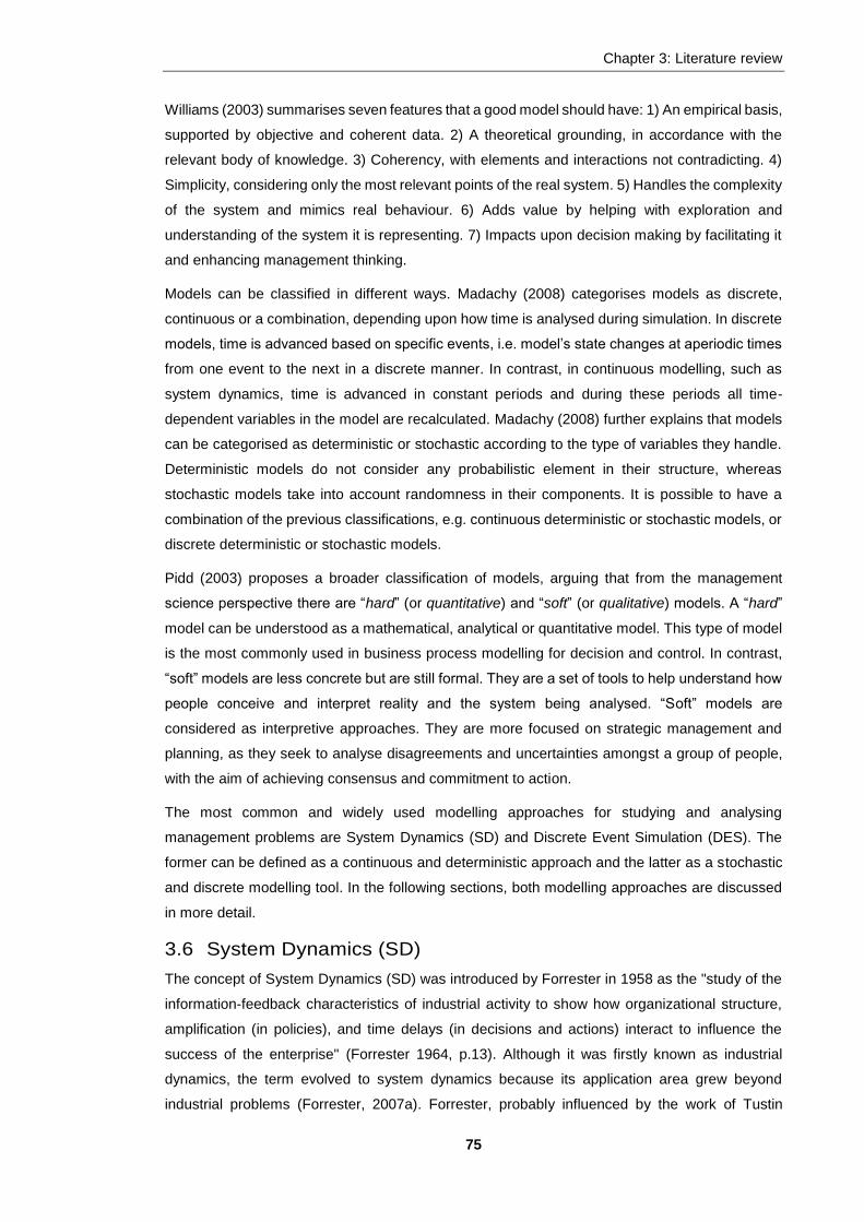
Chapter 3: Literature review
75
Williams (2003) summarises seven features that a good model should have: 1) An empirical basis,
supported by objective and coherent data. 2) A theoretical grounding, in accordance with the
relevant body of knowledge. 3) Coherency, with elements and interactions not contradicting. 4)
Simplicity, considering only the most relevant points of the real system. 5) Handles the complexity
of the system and mimics real behaviour. 6) Adds value by helping with exploration and
understanding of the system it is representing. 7) Impacts upon decision making by facilitating it
and enhancing management thinking.
Models can be classified in different ways. Madachy (2008) categorises models as discrete,
continuous or a combination, depending upon how time is analysed during simulation. In discrete
models, time is advanced based on specific events, i.e. model’s state changes at aperiodic times
from one event to the next in a discrete manner. In contrast, in continuous modelling, such as
system dynamics, time is advanced in constant periods and during these periods all time-
dependent variables in the model are recalculated. Madachy (2008) further explains that models
can be categorised as deterministic or stochastic according to the type of variables they handle.
Deterministic models do not consider any probabilistic element in their structure, whereas
stochastic models take into account randomness in their components. It is possible to have a
combination of the previous classifications, e.g. continuous deterministic or stochastic models, or
discrete deterministic or stochastic models.
Pidd (2003) proposes a broader classification of models, arguing that from the management
science perspective there are “hard” (or quantitative) and “soft” (or qualitative) models. A “hard”
model can be understood as a mathematical, analytical or quantitative model. This type of model
is the most commonly used in business process modelling for decision and control. In contrast,
“soft” models are less concrete but are still formal. They are a set of tools to help understand how
people conceive and interpret reality and the system being analysed. “Soft” models are
considered as interpretive approaches. They are more focused on strategic management and
planning, as they seek to analyse disagreements and uncertainties amongst a group of people,
with the aim of achieving consensus and commitment to action.
The most common and widely used modelling approaches for studying and analysing
management problems are System Dynamics (SD) and Discrete Event Simulation (DES). The
former can be defined as a continuous and deterministic approach and the latter as a stochastic
and discrete modelling tool. In the following sections, both modelling approaches are discussed
in more detail.
3.6 System Dynamics (SD)
The concept of System Dynamics (SD) was introduced by Forrester in 1958 as the "study of the
information-feedback characteristics of industrial activity to show how organizational structure,
amplification (in policies), and time delays (in decisions and actions) interact to influence the
success of the enterprise" (Forrester 1964, p.13). Although it was firstly known as industrial
dynamics, the term evolved to system dynamics because its application area grew beyond
industrial problems (Forrester, 2007a). Forrester, probably influenced by the work of Tustin

Chapter 3: Literature review
76
(1953), suggested the application of concepts commonly used to analyse mechanical and
electrical control systems to study human-management problems.
The concept of SD has evolved to become a methodology for designing, building and applying
simulation models to study and manage highly dynamic and complex systems (Ford et al., 2004).
Coyle (1996) states that SD deals with the time-dependent behaviour of managed systems with
the aim of describing the system and understanding, through qualitative and quantitative models,
how information feedback governs its behaviour. This allows for the design of robust information
feedback structures and control policies through simulation. Sterman (2000) explains that SD is
a method for improving learning in complex systems using “management flight simulators”
(generally computer simulation models) as a representation of reality to help understand dynamic
complexity, identify the sources of policy resistance and design more effective policies. Sterman
also stresses that, in order to be useful, SD simulation models must emulate the behaviour of the
real system so that they respond appropriately, not only in conditions already observed, but also
those not yet encountered.
According to Coyle (1977), Sterman (2000) and Forrester (2007a) SD is an interdisciplinary
methodology because it connects exact and social sciences. SD is based on control theory
developed in mathematics, physics and engineering, but deals with social, economic and
management problems, traditionally studied in the social science field. It is highly supported by
computer sciences as simulation models can be designed and built more easily using computers,
resulting in larger, more robust and complex models that can handle more variables and data.
One of the main features of SD is its ability to represent the dynamics of complex systems as
feedback processes. Forrester (1964, p. 14) establishes that "an information-feedback system
exists whenever the environment leads to a decision that results in action which affects the
environment and thereby influences future decisions". Richardson and Pugh (1981) state that
system dynamics simulation models are useful for managing processes that change significantly
over time and have feedback loops where the information is transmitted. Similarly, Sterman
(2000) argues that all systems, no matter how complex they are, consist of networks of positive
and negative feedbacks, and all dynamics arise from the interaction between these loops. He also
states that the dynamics of a system are determined by its feedback processes, along with stock
and flow structures, time delays and nonlinearities. Stocks depict stored quantities, show the state
of the system and generate the information on which decisions are based. Flows represents the
rate of increase or decrease in stocks.
Dangerfield (2014) summarises the main characteristics of system dynamics models. He argues
that they: 1) model the elements of interest as aggregates or groups, not making any distinction
between individual elements. 2) Regard the dynamics of a system as generally being caused by
endogenous factors, such as internal feedback and interaction between variables. 3) Draw a clear
distinction between resource flows and information flows, where the latter causes the former to
change. 4) Adopt a continuous simulation approach, where the model is simulated at constant
intervals of time. Flows are assumed to be continuous and represented by differential equations.

Chapter 3: Literature review
77
5) Are primarily focused on the behaviour of stocks in the system, represented by integral
equations. 6) Have the ability to handle hard and soft variables, considering the latter as being
relevant to model performance.
Pidd (2003) and Brailsford (2014) set out two different ways in which SD can be used: “soft SD”
and “hard SD”. “Soft SD” is qualitative and focuses on designing conceptual models to represent
feedback structure and complex interactions between variables. This approach is based on
understanding the problem and learning from the complexity of the system. To achieve this
objective, “soft SD” uses different mapping and graphical tools such as mental models, causal
loop diagrams (also known as influence diagrams) and sector maps. It aims to understand the
impact of policies and strategies rather than serving as an analytical tool for prediction or decision
support. “Soft SD” is a tool for learning, communication and debate. “Hard SD” focuses on
developing a computer-based simulation model of the system. Generally, “hard SD” uses the
insights obtained by “soft SD” to build a simulation model. It aims to simulate and analyse the
dynamic of the system and to act as a decision-support tool through the comparison and
assessment of scenarios. “Hard SD” centres its attention on mimicking the behaviour of the
system to compare the effects of new policies or strategies on the system performance. It is also
used as an estimation tool of “alternative futures” by experimenting on critical variables in the
model. As illustrated by Morecroft (2007), the complete quantitative model is “an inference engine
to diagnose performance problems; a virtual world to experience dynamic complexity and
stimulate imagination; and a laboratory to design and test new policies and strategies” (Morecroft,
2007, p.85). Both qualitative and quantitative aspects work together to make SD a methodology
for analysing the dynamic complexity of a particular system. As summarised by Lane (2000), SD
provides hard system models from a soft and interpretative modelling process (cited in Morecroft,
2007, p.150).
SD has been successfully applied to a wide range of areas, both in the public and private sectors,
to study and analyse social and engineering problems. For example, in the public sector it has
been applied to health-care, the military and defence, urban development, road maintenance,
environmental and energy issues, politics, population strategies, government policies, natural
disaster assessment and anti- terrorism policies. In the private sector SD has been used in the
finance sector, aerospace and aviation, construction, mining and oil extraction, energy production
and distribution, manufacturing and industrial engineering and information technology and
systems. (Wolstenholme, 1990; Sterman, 2001; Koelling and Schwandt, 2005; Forrester, 2007b;
Tako and Robinson, 2010; Thompson and Bank, 2010).
3.6.1 System dynamics in project management
SD has been widely applied to project management in different areas, such as large scale projects
in construction, shipbuilding, aerospace, and energy, software development and information
technologies, research and development projects, maintenance, aviation, health-care and the
military and defence. The application of SD models encompasses a broad range of project
management issues. Bendoly (2013) highlights the positive effects that SD and systems thinking

Chapter 3: Literature review
78
can have for project management, especially for understanding the dynamics of systems and their
features.
SD has been used to analyse cost and scheduling overrunning, one of the most common
problems in project management. Reichelt and Lyneis (1999) discuss the main causes of projects
overrunning. Ford et al. (2004) studied constructability reviews to reduce highway project
durations. Eden et al. (2005) compare the measured mile approach with SD to analyse cost
overruns. Park (2005) focuses on resource management to reduce cost and schedule overruns.
Lee et al. (2006b) analyse the impact of negative iterative cycles on construction performance.
Ford et al. (2007) investigate the impact of project controls on cost and schedule overruns. Lee
and Peña-Mora (2007) study the causes and consequences of error and changes in the project
objectives. Peña-Mora et al. (2008) propose a hybrid model SD-DES to improve project
performance. Park and Peña-Mora (2003) and Fard and Pena-Mora (2007) study the effect of
non-value adding activities caused by changes and errors in the project. Han et al. (2013) analyse
the effects of design errors in project costs and schedule.
In the context of risk management, Lyneis et al. (2001) use SD to identify risks and assess the
effects of different processes and organization changes on project performance. Rodrigues
(2001) proposes the use of SD modelling within the PMBOK to provide a framework for managing
project risk dynamics. Dulac et al. (2005) analyse organizational safety culture for safety and risk
management in complex engineering projects. Nasirzadeh et al. (2008) apply SD and fuzzy logic
to analyse and manage risk in construction projects, characterising the imprecise and uncertain
nature of risks.
To analyse the impact of labour in project management, Abdel-Hamid (1989) simulate different
policies for managing human resources in software projects to investigate their effect on project
behaviour. Chapman (1998) studies the impact of changing key project personnel on construction
project duration. Bayer and Gann (2006) examine the causes and effects of workload fluctuations
in a project-based professional service organisation. An et al. (2007) propose a “workforce supply
chain” that recruits, develop and deploy workforce in a timely manner to fulfil project objectives.
Another common application of SD in project management has been to the litigation process.
Williams et al. (1995a) analyse delays and disruptions caused by changes and delays in the
design process. Williams et al. (1995b) examine the impact of delays and in-development product
enhancements in highly parallel and time-constrained projects. Ackermann et al. (1997) evaluate
the cost of delays and disruptions during the channel tunnel project. Howick and Eden (2001)
investigate the consequences of compressing large projects due to client pressure, delays and
disruptions. Cooper et al. (2002) discuss the impact of learning lessons from project to project.
Williams et al. (2003) propose a logical, transparent, auditable and sustainable approach to make
litigation claims for delays and disruptions within the projects. Howick (2003) analyses SD as an
approach for handling delays and disruptions for litigation purpose, pointing out its strengths and
limitations.

Chapter 3: Literature review
79
Other applications of SD in project management include planning and scheduling (Abdel-Hamid,
1993; Coyle, 1996; Ceylan and Ford, 2002; Ford, 2002; Adamides et al., 2004; Han et al., 2014),
the analysis of tipping points (Taylor and Ford, 2006; Taylor and Ford, 2008), the exploration of
the impact of changes and rework during project execution (Love et al., 1999; Love et al., 2002;
Cooper and Reichelt, 2004; Love et al., 2008), the analysis of concurrent projects (Ford and
Sterman, 2003; Yaghootkar and Gil, 2012) and the management of resource allocation (Joglekar
and Ford, 2005; Laslo and Goldberg, 2008; Lee et al., 2008).
A possible explanation of the successful adoption of SD in project management is suggested by
Lyneis and Ford (2007). They argue that planning and managing projects is very challenging,
mainly because project conditions and performance constantly change over time as a result of
feedback responses, principally involving nonlinear relationships and the accumulation of project
progress and resources. Several studies note that traditional project management tools are
inadequate for dealing with the dynamism of complex systems, as these tools conceive a project
statically and focus only on part of the project, (Ford and Sterman, 1998; Reichelt and Lyneis,
1999; Lyneis et al., 2001; Lee et al., 2006a; Lee and Peña-Mora, 2007). These studies also
suggest that given this inefficient management, most projects miss budget and schedule
objectives, requiring additional resources. Rodrigues and Bowers (1996) suggest that SD, in
contrast, can be a suitable approach for analysing dynamic complexity in project management
due to its holistic vision of the project rather than a sum of individual elements, the non-linear
analysis of feedbacks and its flexibility for modelling the dynamic project structure.
Lyneis and Ford (2007) identify four general categories where SD has been applied in project
management: 1) Post-mortem assessments for disputes and learning. SD has been used as a
tool to analyse and assess the performance of a project once it has been finalised, as a post-
project evaluation to determine what went wrong and what the causes were. These kinds of SD
models are commonly used in litigation cases or to learn lessons for future projects. 2) Project
estimating and risk assessment, where SD is applied to estimate the resources and time required
to complete the project under specific circumstances. It is also used to evaluate the impact of
unpredictable but possible events that could affect project performance. Here, SD is used as a
pre-project analysis to explore possible outcomes. 3) Change management, risk management,
and project control. In this case, SD is used as a tool for monitoring, assessing and controlling
the performance of a project by comparing it with the project plan. If some changes or adjustments
are necessary, the model helps to determine the best alternatives and to evaluate possible
consequences. The model is used here as a “during the project” analysis, acting as a monitor or
dashboard. 4) Management training and education, where SD models are used as learning tools
for explaining methodology and for understanding the behaviour and complexity of the system,
acting as laboratories or flight simulators for training project managers.
Summarising, it can be argued that SD is a tool for understanding and managing highly dynamic
and complex systems that has been successfully applied to project management to analyse and
Chapter 3: Literature review
80
solve numerous problems that impact upon the development and performance of a project and
the achievement of its objectives.
3.7 Discrete Event Simulation (DES)
Discrete Event Simulation (DES) is founded on Monte Carlo simulation (Robinson, 2014) and is
a stochastic discrete simulation methodology for modelling systems as networks of queues and
activities as they evolve over time, where the stated variables change only at countable points
over time. The conditions for these activities and the order in which they may occur can be
extremely complex (Law and Kelton, 2000; Brailsford, 2014). Belton and Stewart (2002) explain
that DES models the changes of individual entities in a system of queues, and through the
utilisation of theoretical and empirical statistical distributions to represent variability, the stochastic
nature of the system is represented. To simulate a DES model, a considerable amount of
quantitative data is required, plus the input distributions for all sources of stochastic variation.
Furthermore, as DES simulation is a sampling process, it requires a large number of simulation
runs to obtain better and more accurate results that help the understanding of output distribution
(Brailsford, 2014; Robinson, 2014).
To represent a system, DES uses four elements: entities, queues, activities and resources.
Entities “are the individual elements of the system that are being simulated and whose behaviour
is being explicitly tracked” (Pidd, 2004a, p.64). Each has specific features or attributes that enable
them to be distinguished from other entities and to control their own behaviour (Pidd, 2004a).
Queues are where entities wait for available resources in order to be processed. Cassandras and
Lafortune (2008) point out that in queuing systems three elements are involved: the entities that
are waiting to be treated, the resources which are being waited for and the space where the
waiting is done. Activities are the performance of any kind of work and change entities in specific
ways. “The operations and procedures that are initiated at each event are known as activities and
these activities are what transform the state of the entities” (Pidd 2004a, p.66). Resources are the
system elements that must be available to perform activities. Like entities, they are individual
elements, but their behaviour is not modelled individually. Instead, they are treated as countable
items (Pidd, 2004a). In summary, in a DES model individual entities flow through a certain number
of activities. During the process, the entities have to wait in queues for available resources.
According to Robinson (2014) there are three main features of DES: 1) modelling of individual
entities, 2) time handling, and 3) randomness in the system.
In DES, the system is represented as individual entities that move through a network of queues
and activities (Tako and Robinson, 2014). The entities in the system are distinct objects that are
perfectly traceable, each having their own characteristics that determine what happens to them
(Brailsford, 2014).
Regarding time handling in DES, unlike continuous time simulation, a system is modelled as a
series of “events”, that is the points in the time at which the state of the system changes
(Robinson, 2004). The evolutionary state of the system depends on the occurrence of

Chapter 3: Literature review
81
asynchronous discrete events through time (Cassandras and Lafortune, 2008). In other words,
DES models are simulated in unequal time-steps only when the system state changes (Brailsford,
2014)
An event in the context of discrete-event simulation can be defined as “an instant of time at which
a significant state change occurs in the system” (Pidd, 2004a, p.65). An event can be understood
as occurring instantaneously and producing a transition from one state value to another
(Cassandras and Lafortune, 2008). There are two different types of events that might occur: firstly,
bound or booked events that are programmed to occur at a specific point in time and depend on
a particular action taken and secondly conditional events that cause changes in the system when
certain conditions in the model are met (Pidd, 2003; Robinson, 2004; Cassandras and Lafortune,
2008). According to Robinson (2014) interconnected randomness is the key factor in system
performance and is at the heart of DES modelling.
In DES, the randomness of the system occurs over the length of time an activity takes (Robinson,
2014). Randomness is modelled by sampling activity durations for each entity from probability
distributions (Brailsford, 2014). In other words, to represent the stochastic nature of the system,
DES utilises probabilistic distributions to characterise the unpredictability and complexity of that
system.
According to Brailsford (2014), DES is the most widely practically used modelling operational
research approach. She explains that DES models are often used for comparison of scenarios,
prediction or optimising specified performance criteria and are generally applied at a tactical or
operational level. DES has been widely used for understanding, analysing and improving the
design and operation of systems, but has also been used to help and support strategic decision
making (Robinson, 2014). It has been traditionally used in the manufacturing sector, but has
recently also been applied to the service sector (Tako and Robinson, 2014).
With regard to the specific context of this study, DES has also been used to study and analyse
different problems in process and project management and also to address common issues in
aircraft maintenance.
Fanti et al. (1997) used DES in process management to analyse complex resource sharing and
deadlocks in flexible production systems. They simulated resources interactions and proposed
different control policies to ban or allow specific resource allocation strategies and minimize
deadlocks. Louit and Knights (2001) developed a model using DES to analyse and evaluate
different strategies, aiming to improve the maintenance of mining equipment by identifying the
critical root-factors that impact upon a mine maintenance system and to determine the best
improvement initiatives through testing. Krause et al. (2004) proposed DES as a decision support
tool for shipbuilding to test and evaluate different scenarios in investment planning, scheduling,
and resource planning.
Lu and AbouRizk (2000) proposed a simplified CPM/PERT model for project management to
evaluate different scenarios based on computer simulation and risk analysis. The model

Chapter 3: Literature review
82
incorporates DES into traditional CPM/PERT for modelling entities, their particular attributes and
the points of time (events) where the entities are processed. The model aims to overcome the
limitations of traditional CPM/PERT approaches and to significantly reduce computation time.
Zhang et al. (2002) proposed a model combining DES and the critical path method (CPM) for
construction project scheduling and planning, aiming to enhance modelling capabilities under
complex scenarios and to assist in planning resource allocation policies. In their model, DES is
used to obtain late-time information in addition to resource utilization statistics. Cho and Eppinger
(2005) applied the design structure matrix (DSM) and parallel discrete-event simulation method
for analysing and managing the development of complex design projects. They argued that their
proposed model can be used to increase understanding of the real behaviour of design projects,
to improve project management and to assess and compare planning and execution strategies.
Kouskouras and Georgiou (2007) employed DES for managing a software project. The model
works as a decision support tool for controlling and monitoring the project and to determine the
best planning alternative. Setamanit et al. (2007) developed a hybrid model based on SD and
DES to analyse and assess different task allocation strategies to configure global software
development (GSD) projects. The model also allows for the analysis of the impact that different
factors have on the studied allocation strategies.
With respect to aircraft maintenance applications, and as already discussed in section 3.1,
Bowman and Schmee (2001) proposed a model to mitigate and manage financial risk for a
Maintenance, Repair and Overhaul organization (MRO). Warrington et al. (2002) designed an
aircraft reliability and maintenance model based on DES. Bazargan and McGrath (2003)
proposed a model to improve aircraft availability and maintainability. Weckman et al. (2006)
developed a decision support approach for modelling jet engine life and estimating maintenance
requirement for engine restorations. Allgood, Olama and Lake (2010) designed a DES model
combined with human factor analysis to study, analyse and evaluate performance improvements
for an aviation cargo flow and security inspection system. In their model, they compared different
scenarios by changing several model parameters and then assessing various indicators of the
system’s performance to assess its ability to service current needs and respond to additional
requests. The model helped them to design new inspection requirements and policies without
affecting operational cost or incurring in shipping delays. Horning et al. (2012) developed an
interesting model based on DES to simulate the flight operations of an aircraft fleet and the
resulting maintenance requirements. More recently, Van den Bergh et al. (2013) combined DES
and data envelopment analysis (DEA) to design a model for managing aircraft line maintenance
workforce scheduling.
3.8 Comparison of system dynamics and discrete event simulation
Different authors have studied from different perspectives the differences and similarities between
SD and DES (Sweetser 1999; Brailsford and Hilton 2001; Morecroft and Robinson 2005; 2014;
Greasley 2009; Tako and Robinson 2010; 2014; Brailsford 2014; Han et al. 2014). Given these
reviews, the main differences between SD and DES can be summarised as follows.

Chapter 3: Literature review
83
Modelling structure: although both approaches seek to represent the behaviour of a real system
over time in a simplified manner, their modelling structure clearly differs. In SD, the system is
represented as a set of interconnected stocks and flows modelled in continuous time-steps. The
stocks are used to describe the accumulation of elements, while flows regulate the amount of
resources that enter or leave the stocks. In DES, the system is depicted as individual entities
passing through a series of queues and activities at discrete time intervals. Queues are formed
by entities waiting to be processed, while activities perform changes on entities.
Time handling is one of the main points of difference between SD and DES. In SD, system state
changes are continuous; however, it uses a semi-continuous simulation approach, represented
by differential equations that on a computer are modelled using small constant time steps to
describe the changes in the system state. In DES, system state transitions take place at discrete
points of time that are modelled at asynchronous time steps, when a change in the system (known
as “event”) occur.
Entities perspective: in SD, the elements of a system are modelled as a conglomeration of
elements. There is no distinction between elements and they have the same features, so all that
is measured is their flow through the system, not the specific status of a particular element. SD
models the entities in a global perspective. In contrast, DES keeps track of each element. As each
entity has particular characteristics, it is possible to accurately determine its status and movement
through the system. DES models the entities in an individual perspective.
Modelling approach: SD models are deterministic, where the growth-decay of stocks is modelled
as a delay, usually following an exponential or s-shaped behaviour. DES models are stochastic,
with activity durations represented as random variables, usually based on probability distributions.
Modelling complexity is related to the previous point. SD explains the dynamic complexity of a
system by using feedback structures (deterministic complexity). DES explains it by using several
interrelated random processes (stochastic complexity).
Data requirements: SD models do not use a lot of data as they are more concerned with the
structure of the model, using hard and soft data to model and represent the feedback structure.
In contrast, DES models require a large amount of data to represent the randomness of the
system, to model each individual entity and to maintain the list of events, but can model great
complexity and detail.
Validation: In general terms, SD uses an open-box validation approach, where the structure,
consistency, coherence and meaningfulness of the conceptual and mathematical models must
be checked. However, due to its general perspective and the use of qualitative and quantitative
data, validation in SD can be very subjective, complicated and arduous. DES mainly utilises a
closed-box validation approach, where due to the large amount of data involved in the simulation
process, a plethora of statistical and analytical tools can be used to compare the final results and
behaviour these type of models against the actual results observed in the real system.

Chapter 3: Literature review
84
Application: due to their holistic perspective, SD models are more commonly used at a strategic
level as learning laboratories, providing a broad picture (quantitative and qualitative) of system
behaviour. DES, with its analytical point of view, has been widely used at operational and tactical
level as operation simulators, providing statistical estimations of system performance.
Brailsford (2014) suggests that the main philosophical difference between SD and DES lies in the
way the world is perceived, and therefore how the problem is conceptualised and modelled. She
summarises that while SD is a top-down approach, DES is bottom-up methodology, that is, SD
conceives the world as a system of dynamically interconnected elements and takes a ‘helicopter
view’ of the world, whereas DES, takes a “microscope view”, looking at the system in detail,
analysing variability between individual components.
3.9 Summary
Assessing the literature review focused on the aviation industry, it can be seen that several
approaches have been applied to analyse aircraft maintenance problems, providing different and
valuable proposals for solving them from different perspectives. Due to its direct impact on daily
operations, most of the studies were focused on the line maintenance process, particularly in
managing the workforce and for disruption recovery. Analyses of the heavy maintenance process
aim mainly to address the long-term planning and short-term scheduling of the maintenance
service. However, despite the relevance of the problem, only a few studies attempted to analyse
the uncertainty caused by unscheduled maintenance tasks.
It can be argued that aircraft heavy maintenance services have more than one of the
characteristics of a complex project: uncertainty, number of elements and interaction between
them. It can be argued that each heavy maintenance process is a complex project.
Every project has a certain degree of risk and this is greater for complex projects. Risk, as
discussed previously, is compounded by a latent uncertain event and the consequences, either
positive or negative, for project performance. In terms of heavy maintenance, risk is understood
as the occurrence of unexpected damages or failures, events, which must be corrected by
programming unscheduled maintenance activities which might require additional resources and
tasks hindering the planning and execution of the service. Overrunning costs, delays in the
delivery time and even poor service quality are potential consequences of these unexpected
events.
Uncertainty is inherent in any project and aircraft maintenance is no exception. It cannot be
avoided as it is extremely difficult to predict and control all events on major projects and to possess
all relevant information. Traditionally, uncertainty has been associated with the randomness of an
outcome and described by using probabilities. However, the concept is more sophisticated than
just variability, as it also considers ambiguity, deficiency, imprecision, conflict or absence of
information. These must all be considered to achieve a deeper understanding of uncertainty. In
aircraft maintenance, as in most complex projects, the probability of the occurrence of an

Chapter 3: Literature review
85
unexpected event is unknown in advance and generally a rough assessment is made based on
perceptions or subjective judgements, giving rise to vague and ambiguous estimates.
Similarly to aircraft maintenance studies, two main perspectives have been utilised to study the
planning, scheduling of complex projects under uncertainty: mathematical optimisation models
and computer simulation models. In general terms, the former seeks to minimize delays or budget
overruns, or to maximize resource utilisation, by designing robust and reliable project plans
capable of dealing with the effects of unexpected events. This is usually accomplished by
extending activity duration, increasing the budget or the availability of resources, a practice
commonly called buffering. However, a major drawback of the optimisation models is that they
are usually static and so not able to adapt to changes in the system. Therefore, they are generally
used to define an initial project plan. Simulation has been widely used to characterise, analyse
and predict the operation and evolution of a system over time. Its flexibility enables it to handle
dynamism, irregularity, uncertainty, interrelatedness and complexity. In project management and
aircraft maintenance, simulation has been particularly applied to optimisation and estimation and
as a decision supporting tool. Nevertheless, it has also some disadvantages. It normally requires
a considerable amount of data and computation time and so can be time-consuming.
SD is a flexible simulation approach for studying and managing dynamic and complex systems
characterised by sophisticated interrelations between elements. It has been successfully applied
to project management because of its capacity for analysing projects from a holistic perspective,
representing their dynamism and non-linear relationships, and for handling qualitative and
quantitative data. Most of the SD studies in project management have focused on studying and
analysing project resources and their influence on project performance, the assessment of project
changes and their relationship with project time and budget overruns and the causes and impact
of project delays and disruptions. These studies have used SD throughout the whole life-cycle of
the project, i.e. during the design and planning for estimation and risk assessment, in the
execution as a monitoring and controlling tool and after the close-out for evaluation and learning.
DES is one of the most widely applied simulation approaches. It is used for modelling complex
systems as they change at specific points in time and has the ability to capture in great detail the
condition and flow of each element that passes through the system. In DES, to epitomise the
stochastic nature of the system, the random duration of activities is described by utilising
probabilistic distributions. However, modelling to such a level of detail and complexity requires a
large amount of data, previous knowledge about probability distributions and the performance of
a considerable number of runs of the model. Due to its analytic and comprehensive perspective,
DES has primarily been used at operational and tactical level for estimation and optimisation.
Both simulation methodologies have shown their usefulness for analysing complex systems and
have been extensively used in project management. However, aircraft heavy maintenance is a
highly dynamic process, involving a large amount of scheduled and unscheduled maintenance
tasks and requiring a vast number of resources that are in constant interaction. Moreover,
maintenance services tend to vary significantly between them. For these reasons, it would be

Chapter 3: Literature review
86
more useful and clear to have a broader view of the problem, describing the whole behaviour and
feedback structure of the system rather than giving a detailed perspective of the status and
complex evolution of each maintenance task throughout the maintenance service.
In light of the literature review, it can be argued that little investigation has been carried out into
the effect of unexpected events on aircraft heavy maintenance. Considering the two key aspects
of the problem, the complex interrelationship between the variables involved in the process and
the uncertainty caused by the non-scheduled tasks, it can be suggested that SD provides a
suitable methodology for analysing the impact of unscheduled tasks on delays and disruptions
during the heavy maintenance process.
Despite all the advantages that SD offers to analyse dynamic and complex projects, it is not
exempt from limitations and does not provide a complete solution by itself. Many authors have
pointed out the drawbacks of SD (Jackson, 2001; Tako and Robinson, 2010; Brailsford and Hilton,
2001; Brailsford, 2014), mainly its inability to represent and describe randomness in a system. To
overcome this limitation it will be necessary to support SD by using alternative tools to strengthen
and enrich the proposed solutions. Sterman (2000) remarks that SD modelling does not stand
alone and the best results are achieved in combination with other tools.
In the case of aircraft heavy maintenance, it is particularly necessary to analyse the stochastic
nature of unscheduled tasks and to explore their relationship with different operational and
maintenance variables in order to find a suitable way to estimate them. It has been observed
through experience and in the literature review that a common practice in the airline industry is to
roughly estimate the expected number of non-routine tasks by using a “rule of thumb” based on
expert judgements or in the best case by using average values based on the behaviour of the
fleet.
It is important, therefore, to propose a realistic and rigorous way for estimating the expected
number of non-routine tasks considering not only the variability of information but also other
dimensions of uncertainty such as ambiguity and imprecision. It is proposed to analyse from a
different perspective the uncertainty of unforeseen events that can cause delays to and disruption
of complex projects by using evidential reasoning as an inference process rather than traditional
probability approaches.
It is proposed to combine the system dynamics model with the evidential reasoning model to
assess the impact of unscheduled tasks on the delays and disruptions within the heavy
maintenance. The first model will address the complexity of the process, while the second will
focus on the stochastic nature of the unscheduled tasks.
This research is focused on a particular but common problem in aviation maintenance. However,
delays and disruptions caused by unscheduled tasks are not exclusive to this field and are a
frequent and recurrent problem in other complex projects. Thus, the models, results and learning
developed during this research can be generalised and applied to analyse problems with similar
characteristics.

87
Chapter 4: Methodology and research
design
A current problem in the aircraft maintenance industry has been presented. Its existence and
relevance have been supported by other studies and, through an extensive literature review,
potential opportunity areas and promising methods have been identified. The next step is to define
a formal and systematic process in which this research will be carried out to address the proposed
problem. This chapter aims to formalise and describe the methodology and research design
adopted in this thesis and is structured as follows: firstly, the philosophical bases are discussed
by positioning the ontological and epistemological assumptions considered in this research to
further define the methodological approach adopted. Secondly, the proposed research design is
explained along with its different steps. Thirdly, the two main methods utilised in this research for
analysing the problem are discussed: system dynamics (SD) and the evidential reasoning (ER)
rule. Finally, the research questions in which this research is grounded are presented and
subsequently operationalised to explain how they are going to be addressed.
4.1 Ontological and epistemological basis of the research
Before going any further, it is important to establish the ontological and epistemological
foundations of this research to formalize the type of methodology to utilise. The root of the
dilemma between choosing quantitative or qualitative research is more philosophical than
methodological, since the researcher’s selection of the philosophical assumptions largely
influences the choice of the methodology approach (Dobson, 2002; Krauss, 2005).
According to Burrell and Morgan (1979) social theory can be usefully analysed in terms of four
broad paradigms: functionalist, interpretive, radical humanist and radical structuralist. The
functionalist paradigm considers society to be concrete, real, objective and systemic. Its essential
nature can, therefore, be known and measured to determine human behaviour. Functionalism is
a regulative, rational and pragmatic approach focused on producing useful empirical knowledge.
In contrast, the interpretative paradigm assumes that the social world does not concretely exist,
as it is the result of the subjective experience of individuals. Therefore, its meaning, regularity and
effect on human behaviour is highly variable. Knowledge is based on a set of subjectively
determined concepts and rules. The radical humanist paradigm is focused on finding ways to link
knowledge and action as a way to create change and transcend alienation. Finally, the radical
structuralist paradigm is concerned with understanding social conflicts and contradictions, using
knowledge and action as a way to transcend domination (Barley, 1980; Morgan, 1980).
Each of these paradigms can be classified according to their location within two meta-theoretical
dimensions: the nature of social science and the nature of society. Both dimensions are
characterised by opposing perspectives: objective vs. subjective in the case of the former and

Chapter 4: Methodology and research design
88
regulation vs. change in the case of the latter. The four paradigms group various schools of
thought, with diverse approaches and standpoints, but share common fundamental assumptions
about the nature of the reality that they address (Morgan, 1980). Burrell and Morgan (1979)
conceptualise the subjective and objective perspectives of social sciences in terms of four
philosophical assumptions related to ontology, epistemology, human nature and methodology.
Ontology refers to assumptions and convictions about the essence, nature and existence of the
world or a certain phenomenon (Burrell and Morgan, 1979; Mingers and Brocklesby, 1997;
Meredith, 2001; Rotaru et al., 2014). Nominalism, also known as conventionalism, conceives the
social world as a cognitive and artificial creation formed exclusively by names and labels. It does
not acknowledge any real structure and is defined by Burrell and Morgan (1979) as a subjectivist
approach. On the other hand, realism, located in the objectivist perspective, considers that reality
exists even if there is no awareness of its presence as it is created by tangible and immutable
structures external to human cognition (Burrell and Morgan, 1979).
Epistemology is the theory of knowledge. It comprises the study of the nature, bases and scope
of acquired knowledge, how it is used to understand the world or a particular phenomenon and
how it is transmitted to others (Burrell and Morgan, 1979; Mingers and Brocklesby, 1997;
Meredith, 2001; Rotaru et al., 2014). Burrell and Morgan (1979) considers anti-positivism, or
interpretivism, as part of the subjectivist approach and positivism as objectivist. Anti-positivism
assumes that the social world is relativistic and is only understood with reference to the individuals
involved in the studied phenomena. This perspective asserts that the social sciences are not able
to generate objective knowledge. Positivism, on the other hand, attempts to describe the social
world based on observed causal relationships and regularities. This epistemological approach is
characterised by the ability to verify hypothesis through experimentation and therefore it
dominates the natural sciences.
Human nature encompasses the relationship between individuals and their environment and how
the individual is perceived in a given social-scientific theory (Burrell and Morgan, 1979). Burrell
and Morgan (1979) identify two opposite approaches: voluntarism, which is subjectivist and
determinism, which is objectivist. Voluntarism regards individuals as creative and autonomous
beings, constructing and controlling their own environment. Determinism considers individuals
and their experiences and activities as products of the environment conditioned by external
situations.
These three previous philosophical assumptions shape and influence the methodological
approach that refers to the systematic way in which knowledge is pursued and acquired (Burrell
and Morgan, 1979; Smyth and Morris, 2007). The ideographic standpoint, which can be classified
as subjectivist, assumes that the social world can only be understood by considering the
relationship of the individual with their environment in order to gain insight about the subject under
investigation. The objectivist nomothetic approach considers that social sciences can be studied
using systematic and rigorous techniques focused on analysing data and testing hypotheses
(Burrell and Morgan, 1979).

Chapter 4: Methodology and research design
89
The two proposed methods for this research are quantitative approaches and as such are located
in the functionalist paradigm according to the (Burrell and Morgan, 1979) framework. However,
they are also able to consider and handle subjective information. With this in mind and given the
interpretative nature of the models (mental and formal), it may be more appropriate to place them
somewhere between the interpretative and functionalist paradigms.
Considering the philosophical essence of the problem, as per the ontological dimension, this
research assumes a realistic stance, regarding organizations and their problems, in this particular
case airlines and MROs, as real, concrete and formal structures which can be observed and
studied, where their relevant problems can be analysed and measured.
At first glance, given the conditions of the problem and considering the characteristics of the
proposed methods, it appears that this research makes a positivist epistemological assumption,
takes a deterministic approach towards human nature and adopts a nomothetic methodology.
However, assuming this position might be extreme, inflexible and unrealistic, excluding
individuals' interpretations about the problem and considering that the decision maker has no
influence on the environment and thus on the problem. Project overruns, for example, would be
presumed to depend exclusively on external factors, with managers' decisions and perceptions
not affecting project performance.
It would be more fruitful to adopt an intermediate position between the positivist and interpretivist
approaches with less radical assumptions about human nature, allowing for a more flexible
methodological approach. This view is supported by Gioia and Pitre (1990), Weaver and Gioia
(1994) and Remenyi et al. (1998) who agree that rather than assume a dichotomy between
objective-subjective, these approaches should be considered as complementary, with their
overlapping boundaries offering a transition across paradigms. In the same vein, Blatter and
Haverland (2012) propose an “epistemological middle ground” that rejects fundamentalist and
extreme epistemological positions. This suggests that social science research is based on
thorough reflection on the relationship between empirical evidence and abstract concepts and
assumes them to be commensurable.
Likewise, the structuration theory of Giddens (1984) proposes that the objective and subjective
perspectives are intertwined and it is not possible to separate them. This theory allows for the
articulation of a set of relationships amongst the competing perspectives, where reality arises
from the constant interaction between structure and meaning, rather than one or the other
(Weaver and Gioia, 1994; Mingers and Brocklesby, 1997).
Similarly, critical realism (Bhaskar, 1975, 1979, 1994) describes a coexistence of intransitive and
transitive objects of knowledge, with the former describing real entities that exist independently
to individual perspective and the latter resulting from individual experience, representations and
descriptions used to produced knowledge. Social theories, therefore, cannot be purely descriptive
or evaluative. There must be balance between them, as facts and values cannot be separated
(Mingers and Brocklesby, 1997; Mingers, 2000, 2003, 2006). Critical realism provides a “position
that would allow the combined use of the objectivist worldview that is based on the assumption

Chapter 4: Methodology and research design
90
of existence of ‘an objective reality which can be measured and described’ and a more subjectivist
position that allows ‘the mind of the decision maker’ to interpret the reality based on the available,
including value-laden, data” (Rotaru et al., 2014, p.98).
Taking a more flexible and inclusive philosophical position on the objective-subjective dichotomy
can allow for a multi-methodological position, where “methods and techniques from the original
competing paradigms may be combined without the agent having to constantly adjust their
philosophical position depending upon whichever method is being used at any time” (Mingers and
Brocklesby, 1997, p.498). This position can enrich research by using distinct methods and tools
to overcome the individual weaknesses of particular methods. Mingers (2003) highlights the
benefits of considering a multi-methodological approach. The real world is multidimensional and
material, social and personal factors should all be considered. Different ways of appreciation,
analysis, assessment, and action are required. Such a wider perspective may enhance the
richness and reliability of results.
In the light of this, it is proposed to use an exploratory perspective based on a case study rather
than a nomothetic approach. A case study seems the most suitable approach as it can help to
gain insight into the problem by describing and testing the initial hypothesis via a holistic in-depth
exploration of the dynamics, complexity and uniqueness of the organization and the project in
question, using both quantitative and qualitative data (Eisenhardt, 1989; Yin, 2003; Simons, 2009;
Farquhar, 2012). The exploratory approach is proposed as a comprehensive and systematic
method for improving the understanding of a particular phenomenon, especially when little is
known about it, by determining and examining significant issues and crucial variables and defining
the necessary questions and hypotheses (Eisenhardt, 1989; Stebbins, 2001; Yin, 2003; Streb,
2010). In this research, the initial empirical assumptions regarding the problem were further
explored and supported using a wide-ranging literature review, leading to the formulation of the
research questions and supporting the use of the proposed methods.
4.2 Research design
This research has an empirical motivation based on personal experience in the airline industry
and supported by the insights of various authors and experts in the field. From the evidence
presented thus far, it can be argued that delays and disruptions during the execution of aircraft
heavy maintenance services is a real, frequent and relevant problem with important economic
and operational consequences for both airlines and MROs. Schedule and budget overruns in
maintenance checks stem from the complexity of managing resources and the occurrence of
unplanned maintenance tasks. The literature review has shown that these features and problems
are not exclusive to the heavy maintenance process but are common in complex projects across
different industries such as construction, engineering, manufacturing and software development.
Prior studies have noted the deficiency of the traditional project management methods when
dealing with highly dynamic, unstable and uncertain projects. To overcome these limitations,
simulation has been applied as an alternative approach for studying complex projects, due to its
capability to capture the development of a project over time. System dynamics (SD) has proved

Chapter 4: Methodology and research design
91
to be a useful method for analysing the operation and behaviour of complex and dynamic projects,
especially for conceptualising projects from a holistic perspective and for capturing the dynamism
of elements and the relationships between them.
Considering the main features of the problem and the ability of SD to analyse dynamic and
complex systems, it is suggested to use SD for considering the effect of unscheduled tasks on
delays and disruptions within aircraft heavy maintenance checks. However, it has been shown
that SD has limited capabilities for dealing with randomness in the system. To cope with this
drawback, it is proposed to use the evidential reasoning rule as a complementary tool to handle
uncertainty.
The SD model helps to analyse the interrelationship of scheduled and unscheduled tasks and its
impact on delays and disruptions and also to explore the effect on project performance of the
occurrence and discovery of damage and discrepancies during unscheduled tasks. The ER rule
model complements the SD model by estimating unscheduled maintenance tasks by analysing
historical data related to the usage and maintenance of an aeroplane, taking into account its
importance and quality. The enhanced SD model can be used as a decision supporting tool by
exploring different policies and strategies for the planning and control of the maintenance service.
Research design is the coherent and logical process of merging the research elements, aiming
to successfully address the research problem. It considers the creation, collection, organisation,
measurement, analysis and interpretation of data (Vaus, 2001; Perri and Bellamy, 2012). In this
thesis, to accomplish the research objectives, an iterative research design process is proposed,
based on the research frameworks proposed by Eisenhardt (1989), Yin (2003), Hernández
Sampieri et al. (2010) and Creswell (2014), and using as a reference the modelling processes
suggested by Forrester (1994), Sterman (2000) and Pidd (2004a). The research design consists
of eight phases as described below:
(1) Problem structuring: based on experience and the literature review, the process and the
problem are explained and contextualised, the relevance of the problem is supported and
the suitability of the proposed methods is discussed. The aim of this phase is to define the
problem and its main features, delineate the research objectives and scope, and define the
research questions.
(2) Conceptual model: the SD model refers to the initial causal-loop diagram that depicts the
main components and their relationships, and the possible causes of the problem. The ER
rule model describes the basic configuration for aggregating the variables to estimate the
non-routine rate. The aim of these preliminary models is to aid the gathering of data.
(3) Data collection: where qualitative and quantitative data is collected, organised and analysed.
Continuous discussions with experts and practitioners are used to validate the dynamical
hypothesis and to improve the causal loop diagrams. Maintenance and operational records
are used as input variables for building the ER rule model to analyse the uncertainty of the
non-routine tasks, and these records are also used to build and test the SD simulation model.

Chapter 4: Methodology and research design
92
(4) Model refining: the improvement of the initial concepts by including additional information
from the previous step and taking into account experts’ modifications to describe the problem
more accurately. For the SD model, considering adjustments in the variables, relationships
and feedback loops to improve the structure of the model. For the ER rule model, considering
the inclusion of or changes in the input variables.
(5) Formulation and simulation: describing the transition from the conceptual model to a detailed
mathematical model. For the SD model, considering the development of the stock-flow
diagram and the definition of its equations to finally complete the simulation model. For the
ER rule model, referring to the application of the ER rule process to combine different pieces
of evidence to estimate the non-routine rate.
(6) Model validation: assessing if the model complies with its intended purpose. For the SD
model, a white-box validation approach is considered as this step in SD could be very difficult
and subjective. The model is tested and verified throughout the modelling process, with
reference to the opinions of experts regarding its meaningfulness. Verifying the structure of
the model and the mathematical equations and evaluating the results. For the ER model, a
black-box validation approach is carried out where the estimated non-routine rates are
compared with the observed values to assess the model performance. Additionally, a
sensitivity analysis is carried out to determine the effect of certain variables on model
efficiency.
(7) Scenario analysis: the use of the models for building and comparing scenarios to allow the
testing of different policies and for learning the behaviour of the system under certain
circumstances, for instance, to assess the impact of different resource allocation strategies
and the effect of the occurrence and discovery of discrepancies on project performance.
(8) Findings and conclusions: with the results of both models and the knowledge gained during
the investigation process, the research questions can be answered and relevant findings can
be discussed, stating also the limitations of the study and suggesting potential further
research.
4.3 System dynamics modelling
System dynamics comprises the development of qualitative and quantitative models. Causal loop
diagrams are used to describe the structure of the system and the relevant interrelation between
its elements. Stock and flow diagrams are used to build a dynamic model and simulator depicting
the evolution and performance of the system through the time.
SD models are useful for coping with dynamic complexity resulting from the sophisticated
relationship between the elements of the system, where a change in the system can have an
impact elsewhere in the short-, medium- or long- term. However, the cause-effect relation is not
always obvious and sometimes even counterintuitive (Sterman, 2001).
Moreover, SD models are not intended to predict or forecast the future. They serve to build
scenarios and explore potential futures that may unfold if the assumptions behind the scenarios

Chapter 4: Methodology and research design
93
turn out to be true. They are used to test the consequences of choosing certain strategies or
policies, to anticipate problems, reveal surprises and hidden pitfalls (Morecroft, 2007).
4.3.1 Causal loop diagrams
A causal loop or influence diagram is a graphical representation of the main system structure,
depicting the interrelation between the elements within the system. Causal loop diagrams, (CLDs)
through the abstraction and representation of mental models of individuals and teams, help to
change the problem perspective from a cause-effect relation to a complex structure formed by
feedback loops. They are particularly useful for enhancing the understanding of a problem by
capturing potential causes of dynamics and feedback, and for illustrating qualitative and
quantitative information (Sterman, 2000; Morecroft, 2007; Brailsford, 2014).
CLDs are used to describe cause and effect relationships between the variables and to represent
the feedback structure of the system. The cause-effect relation consists of two or more variables
connected by arrows, while an interconnected array of arrows and variables depicts the feedback
process. The basic elements in the CLDs are: variables, causal links, link polarity, loops, loop
identifier and delays, as shown in Figure 4-1.
Variables are the elements in the system that change due to certain stimuli outside or inside.
Causal links illustrate the direction of the causal effect between the variables and are represented
using arrows. Link polarity describes the direction of change when independent variables change
and is depicted by a positive (+) or negative (-) symbol. A positive or negative link means that
when the cause increases or decreases the effect will change accordingly. Link polarities describe
the structure of the system rather than the variable’s behaviour as they explain what would
happen if there was a change, not what actually is happening (Sterman, 2000).
A loop refers to a closed chain of cause and effect (Madachy, 2008) in which a cycle is completed
when the variable is influenced by the change initially triggered by it. According to its effect, there
are positive and negative loops also called reinforcing or balancing loops respectively. A positive
or reinforcing loop acts as an amplifier or a reinforcing mechanism of growth: for example, an
increase in one variable will eventually lead to a significant boost of that variable. In contrast, a
negative or balancing loop acts as a controller or a mechanism of equilibrium: for instance, an
increment in one variable will eventually lead to a reduction of that variable. The main reinforcing
and balancing loops in the CLD are depicted by using a loop identifier, which must have the same
direction of the loop that it is describing. It should also be numbered and include a brief textual
description (Dangerfield, 2014).
Delays are usually represented as two dashed lines crossing a causal link indicating a lag in the
cause-effect relation between two variables, i.e. if there is a delay, the cause will take longer to
have an effect (Morecroft, 2007).

Chapter 4: Methodology and research design
94
Figure 4-1 Causal loop diagrams notation
Figure 4-2 shows a simple example of a causal loop diagram representing changes in population.
The diagram is formed by two loops, one reinforcing and one balancing. For instance, if average
fertility increases, the birth rate will increase too leading to a growth in the population, which in
turn will cause a further rise in the birth rate, causing a surge in the population, closing the
reinforcing loop. If population grows, death rate will also increase. This increment in the death
rate will cause a reduction in the population, balancing this loop. However, the death rate is
affected by the average life time expectancy, where if the latter increases, there will be fewer
deaths and if it decreases, more deaths will be expected.
Figure 4-2 Causal loop diagram example: the dynamics of population. Based on (Sterman,
2000, p.138)
Different authors have suggested significant benefits of CLDs. Some even consider CLDs as a
separate method from SD, highlighting its capacity to generate insight about the system and its
feedback structure, materialise and communicate mental models, create consensus and help
problem solving, even without using quantitative models and computer simulation (Wolstenholme,
1993; Ballé, 1994; Sherwood, 2011; Merrill et al., 2013).
4.3.2 Stock and flow diagrams
Though CLDs are very useful to broaden the conceptualising of the problem and to improve the
understanding of the system and its feedback structure, they are not able to capture the stock
and flow structure of the system and fail to show the changes and performance of the system
through the time (Sterman, 2000; Morecroft, 2007). The CLDs are generally used to develop the
Variable 2 Variable 3
Variable 1
+
++
R
R
B
Reinforcing loop
(Positive loop)
Balancing loop
(Negative loop)
Birth rate Population Death rate
Average fertility
rateAverage lifetime
+ -
+ +-+
R B
Causal link
Link polarity
Variable
Delay
Loop
Loop Identifiers

Chapter 4: Methodology and research design
95
stock-flow diagrams, which are an essential step for building a quantitative SD model (Brailsford,
2014).
Stock-flow models resemble a hydraulic system formed by connections of tanks, pipes and
valves, where a homogeneous mass of elements flows through the system. A stock and flow
network consists of four main components, shown in Figure 4-3: 1) Stocks, represented by
rectangles, serve as containers to accumulate the elements that flow through the network. 2)
Flows, represented by a thick arrow, describe the movement of elements across the network.
When an arrow points towards a stock, it adds elements and is called inflow. When the arrow
emerges from the stock, it drains elements out of it, known as outflow. 3) Valves or rates are
located in the middle of a flow to regulate or control the movement of elements in the network. 4)
Clouds represent the initial and final points of the flow. Whatever is beyond these limits is out of
the scope of the model (Sterman, 2000; Morecroft, 2007; Dangerfield, 2014).
In addition to these four components, two supplementary elements are required to describe the
feedback structure of the system, causal links and auxiliary variables (also known as converters).
The former are represented by a light arrow, similar to the causal loop diagram, describing the
influence of one variable on another. The latter is an intermediate variable intended to represent
something planned or desired, a target or a management goal. Once all the components are
integrated, the stock-flow diagram has the ability to represent the two fundamental concepts of
SD theory: stocks and flows, and feedback (Sterman, 2000).
Figure 4-3 Stock and flow diagram notation
Figure 4-4 illustrates an example of a stock and flow diagram, depicting population dynamics. The
population stock represents the accumulated number of individuals at a particular point in time.
Total population increases through the number of births per unit of time and decreases by the
number of deaths in the same period. The number of births depends on two variables: the number
of population members and the fractional birth rate, which is the expected number of births per
capita. In a similar way, the number of deaths results from population size and fractional death
rate. The fractional birth and death rates depend on the relation between population size and
carrying capacity. The latter expresses the maximum capacity of the environment to support a
certain population, for instance because of availability of food or physical space.
Valve
Flow
Cloud
Stock
Causal link
Auxiliary variable

Chapter 4: Methodology and research design
96
Figure 4-4 Stock-flow diagram example: the dynamics of population. Based on (Sterman, 2000,
p.285)
4.3.3 System dynamics equations
In theory, System Dynamics is a constant time advance methodology, but in practice this can only
be achieved using a semi-continuous simulation, based on small time steps represented by
differential equations (Dangerfield, 2014). Modelling in finely sliced time steps is a technical and
computational strategy to establish the time units in which the system evolves, in other words, the
stocks are updated according to their related inflows and outflows to yield a new system state at
every time step (Morecroft, 2007). The smaller the time step (dt) the more precise the model will
be. However, it will also increase computation load and the risk of round-off and truncation error,
making it important to define an appropriate dt according to the model features. Morecroft (2007)
suggests using a dt for no longer than a quarter of the smallest time unit in the model.
The final step to complete the quantitative model is to transform the stock-flow diagrams into
equations. Stocks and flows have a precise and unambiguous mathematical meaning. Stocks
accumulate or integrate their flows, while a flow depicts the rate of increase or decrease of a
stock. The status of a stock is represented by an integral equation from an initial time t0 to the
current time t, considering the stock level at t0 and the difference of the inflow and outflow between
t0 and t, as shown in equation (4-1). Correspondingly, the net rate of change in a stock is given
by a differential equation describing the difference between the inflow and outflow at a particular
point in time, presented in equation (4-2). The flows are equations in terms of the stock and other
state variables and parameters (Sterman, 2000).
𝑆𝑡𝑜𝑐𝑘(𝑡) = ∫ [𝐼𝑛𝑓𝑙𝑜𝑤(𝑡) − 𝑂𝑢𝑡𝑓𝑙𝑜𝑤(𝑡)]𝑑𝑡𝑡
𝑡0
+ 𝑆𝑡𝑜𝑐𝑘(𝑡0) (4-1)
𝑑𝑆𝑡𝑜𝑐𝑘(𝑡)
𝑑𝑡= 𝐼𝑛𝑓𝑙𝑜𝑤(𝑡) − 𝑂𝑢𝑡𝑓𝑙𝑜𝑤(𝑡) (4-2)

Chapter 4: Methodology and research design
97
Every component in a stock-flow diagram is defined by an equation, a parameter or a graphical
function. It is worth mentioning that each component in the model is associated with its respective
units to help the representation and description of the model. Therefore, it is very important to
conduct a dimensional analysis throughout the modelling process to ensure the consistency of
units and measures.
Transforming a qualitative causal loop diagram into a complete and robust system dynamics
model and simulator that describes as closely as possible the system and its main troubles
requires experience and takes a lot of time and effort, but the result is much more than a diagram
or a static analytical solution. It is an inference engine to diagnose performance problems, a virtual
world to explore dynamic complexity and stimulate learning and a laboratory to design and
experiment new policies and strategies (Morecroft, 2007).
4.3.4 Validation
As described in the literature review, a model is a representation of a real or conceptual system
that aims to analyse and understand that system. In management science, models are used to
understand, improve and manage real systems and as a decision support tool for testing
strategies and policies in the system. A model’s definition has two main elements: the real system
and the model, where the main objective of the model is to represent in the best way the real
system. However, important questions arise. How to assess the quality and accuracy of the
model? How to be sure that model is representing the real system? How to measure if the model
is accomplishing with its objective and if it is really useful?
Pidd (2003) points out that validation is not as straightforward as it seems, and highlights the
importance of the epistemological perspectives during the model assessment. Citing Déry et al.
(1993) he presents three different standpoints. First, the philosophical, which describes that the
model should be based on objective research, rigorously tested, expressed mathematically,
shown to be useful and should pass crucial tests designed to show its adequacy. Second, the
historical perspective, which considers that validation changes in time and location and refers to
the acceptability of the model to the expert community who are operating with a dominant
paradigm. Finally, the sociological perspective, strongly related to the previous, assesses the
validity of the model according to its acceptance, understanding and usefulness for the intended
community.
Three terms are commonly used during the validation process: validity, credibility and
acceptability. Validity expresses the accuracy of the model to represent the real system.
Credibility describes the willingness of the users to take decisions based on the information
obtained from the model. Acceptability includes the model and the whole modelling process, but
also the relation between the modeller and the user and can be understood as the result of the
validity and credibility (Robinson and Pidd, 1995).
Validation is the process that ensures that a model is suitable and adequate for the purpose for
which it was built (Pidd, 2003; 2004b). Validity and testing is the process of confidence building

Chapter 4: Methodology and research design
98
amongst those who will use the model (Forrester and Senge, 1980; Sterman, 2000). However a
thorough and complete validation that ensures the model is fully correct and exactly represents
the real system is impossible. It is, therefore, important to bear in mind that the validation process
has certain limitations (Pidd, 2004a; Sterman, 2000).
It would be impractical to carry out an assessment once the model has been completed. As the
previous definitions stated, validation is a process not just a single step and therefore should be
performed at different stages during modelling. In this regard, Pidd (2003) emphasises that
assessment and validation are activities that should be performed at every stage of the simulation
project. Morecroft (2007) adds that validation includes different tests that need to be performed
throughout the modelling process with the aim of assessing the quality of both the model and the
model building process. He proposes three categories of tests that have been proved particularly
useful in practice: tests of model structure, tests of model behaviour and tests for learning.
Model structure tests help to evaluate if the feedback structure and equation formulations of the
model are consistent with the available facts and descriptive knowledge of the real system. The
model behaviour tests compare and assess the results of simulation with real system behaviour.
Tests for learning are intended to evaluate if the model users have learnt and gained insight about
the structure and behaviour of the system (Morecroft, 2007). Recalling the idea that a full
validation is impossible, Morecroft (2007) remarks that these tests do not prove whether a model
is valid in the sense of being the perfect depiction of the real system. They can, however, when
used in combination during the modelling process, demonstrate to modellers and clients that the
model is of acceptable quality to meet the intended purpose, providing a reliable basis for
understanding and analysis.
Taking into consideration the previous definitions and philosophical standpoints, it is worth noting
that during the validation process at least two points must be ensured: firstly, that the model
should represent and depict the real system as closely as possible and secondly, it has to be
meaningful, relevant and useful for the user. In order to achieve these purposes, the validation
must be performed in different steps throughout the modelling process.
Considering the validation tests suggested by Morecroft (2007), it is necessary for this particular
project to firstly verify the structure and design of conceptual models with reference to the experts
in the field, i.e. through feedback sessions to revise, discuss and improve the conceptual models
in order to capture and include the relevant missing points of the problem and ensure that the
structure and representation of the model is consistent with the knowledge and perception of the
system. Later, during the design and building of the stock and flow model and also in the
development of the ER rule model, the mathematical equations must be reviewed and verified to
ensure that they are coherent in characterising the problem and dimensionally have a proper
meaning compared with what they represent in the real world. Additionally, it is necessary to run
more tests under extreme conditions, to see if the results of the equations make sense when their
inputs take extreme values. The next set of tests consists of evaluating overall system
performance. Here, it is necessary to use real data, i.e. maintenance and operational records, to

Chapter 4: Methodology and research design
99
compare with estimated results obtained throughout the model. Finally, it is necessary to review
the results with reference to expert opinion, check if they match overall system behaviour and,
through building scenarios, evaluate the usefulness, learning and benefits to users obtained by
using the model.
4.4 Evidential Reasoning rule
The evidential reasoning (ER) rule is a general conjunctive probabilistic reasoning process for
combining independent pieces of evidence, taking into account their weights and reliabilities. The
ER rule is established as a rational and rigorous reasoning method rather than a model to explain
human judgements. The ER rule explains that the combined degree of belief in which two pieces
of independent evidence jointly support a proposition is formed by two parts: the bounded sum of
their individual support and the orthogonal sum of their collective support (Yang and Xu, 2013).
It has been demonstrated by Yang and Xu (2013) that the ER algorithm (Yang, 2001; Yang and
Xu, 2002; Yang et al., 2006) and Dempster’s rule in the theory of evidence (Dempster, 1967;
Dempster, 1968; Shafer, 1976) are special cases of the ER rule. In the case of the ER algorithm,
the reliability is equal to the weight and the weights are normalised for all pieces of evidence. In
Dempster’s rule, each piece of evidence is considered fully reliable.
One of the advantages of the ER rule is that it can be used to combine different pieces of evidence
regardless of the order of aggregation and without affecting the final results. This feature is due
to its being based on the orthogonal sum operation and therefore it acquires the basic properties
of being associative and commutative (Yang and Xu, 2013; Yang and Xu, 2014). Furthermore,
through the use of a novel reliability perturbation analysis, the ER rule can be applied to combine
multiple pieces of evidence that are fully reliable but highly or completely conflicting, overcoming
in this way the non-definition and counter-intuitive drawbacks of Dempster’s rule (Zadeh, 1986;
Murphy, 2000; Haenni, 2005; Huynh et al., 2006).
In the ER rule, three elements are necessary when combining two pieces of evidence: their belief
distributions, weight and reliability.
Firstly, a piece of evidence is represented by a belief distribution (BD) that is defined on the power
set of the frame of discernment, which is a set of hypotheses that are mutually exclusive and
collectively exhaustive, thus allowing the assignment of basic probabilities not only to singleton
hypotheses but also to any of their subsets (Yang and Xu, 2013). A belief distribution is
considered as the most natural and flexible generalisation of conventional probability distribution
as it resembles the human rational process, allowing inexact reasoning at whatever level of
abstraction (Gordon and Shortliffe, 1985). Particularly, a BD is equivalent to a conventional
probability distribution when basic probabilities are only assigned to singleton hypotheses (Yang
and Xu, 2013).
Weight represents the importance of a piece of evidence based on the decision maker’s
preferences over the evidence, whereas reliability measures the quality of a piece of evidence to
provide correct assessment of or a solution to a given problem. While weight is subjective,

Chapter 4: Methodology and research design
100
reliability aims to be an objective measurement. The former relies on who makes the judgement,
whilst the latter assesses the evidence independently of who may use it (Smarandache et al.,
2010). Yang and Xu (2014) explain that weight and reliability are the same if all the pieces of
evidence are measured in the same joint space. However, when the different pieces of evidence
are gathered from different sources and measured in different ways, the weight and reliability are
dissimilar. Additionally, Yang and Xu stress the importance of the part that the weight and
reliability of all pieces of evidence play in the inference process. Therefore, they need to be
estimated with care and rigour.
In the ER rule, these three elements are used to define what is known as a weighted belief
distribution with reliability (𝑊𝐵𝐷𝑅), where 𝑚𝑗 represents the 𝑊𝐵𝐷𝑅 of a particular piece of
evidence 𝑒𝑗, and 𝑗 is the 𝑗𝑡ℎ number of independent pieces of evidence, as expressed in equation
(4-3) (Yang and Xu, 2013):
𝑚𝑗 = {(𝜃, �̃�𝜃,𝑗), ∀𝜃 ⊆ 𝛩; (𝑃(𝛩), �̃�𝑃(𝛩),𝑗)} (4-3)
Considering that 𝛩 is a set of mutually exclusive and collectively exhaustive propositions referred
as a frame of discernment, and that 𝑃(𝛩) represents the power set of 𝛩 consisting of 2𝛩 subsets
of 𝛩; then �̃�𝜃,𝑗 measures the degree of support for a proposition 𝜃 from evidence 𝑒𝑗 with both the
weight and reliability of 𝑒𝑗 taken into account, as defined in equation (4-4) (Yang and Xu, 2013;
Yang and Xu, 2014):
�̃�𝜃,𝑗 = {
0 𝜃 = ∅𝑐𝑟𝑤,𝑗𝑚𝜃,𝑗 𝜃 ⊆ Θ, 𝜃 ≠ ∅
𝑐𝑟𝑤,𝑗(1 − 𝑟𝑗) 𝜃 = 𝑃(Θ)
(4-4)
where 𝑚𝜃,𝑗 = 𝑤𝑗𝑝𝜃,𝑗 is referred to as a basic probability mass, 𝑐𝑟𝑤,𝑗 = 1 (1 + 𝑤𝑗 − 𝑟𝑗)⁄ is a
normalisation factor, which is uniquely determined to satisfy ∑ �̃�𝜃,𝑗 + �̃�𝑃(Θ),𝑗 = 1𝜃⊆Θ given that
∑ 𝑝𝜃,𝑗 = 1𝜃⊆Θ , and 1 − 𝑟𝑗 represents the unreliability of evidence 𝑒𝑗.
Finally, the combined degree of belief in which two independent pieces of evidence 𝑒1 and 𝑒2
jointly support 𝜃, denoted by 𝑝𝜃,𝑒(2), is generated by the orthogonal sum of their weighted belief
distributions with reliability and represented by �̂�𝜃,𝑒(2), given as follows (4-5) (Yang and Xu, 2013;
Yang and Xu, 2014):
𝑝𝜃,𝑒(2) = {
0 𝜃 = ∅�̂�𝜃,𝑒(2)
∑ �̂�𝐷,𝑒(2)𝐷⊆Θ
𝜃 ⊆ Θ, 𝜃 ≠ ∅
�̂�𝜃,𝑒(2) = [(1 − 𝑟2)𝑚𝜃,1 + (1 − 𝑟1)𝑚𝜃,2] + ∑ 𝑚𝐵,1𝑚𝐶,2
𝐵∩𝐶=𝜃
∀𝜃 ⊆ Θ
�̂�𝑃(Θ),𝑒(2) = (1 − 𝑟2)(1 − 𝑟1)
(4-5)

Chapter 4: Methodology and research design
101
From equation (4-5) it can be seen that the combined degree of belief of the two pieces of
evidence is formed by two parts: the bounded sum of their individual support (the first term of the
equation in square brackets) and the orthogonal sum of their collective support (the last term of
the equation). The first term refers to the sum of the degree of individual support of the basic
probability mass (or weighted belief distribution) 𝑚𝜃,1 from the first piece of evidence 𝑒1 restricted
by the unreliability (1 − 𝑟2) from the second piece of evidence 𝑒2, with its counterpart, i.e. the
degree of individual support 𝑚𝜃,2 from 𝑒2 limited by (1 − 𝑟1). In other words, the first term of the
ER rule indicates that the higher the reliability of a piece of evidence, the less opportunity it leaves
for other evidence to provide its information. The second term of the ER rule denotes the
orthogonal sum of the collective support of the evidences, which measures the degree of
intersected or heterogeneous support for the proposition 𝜃 from both pieces of evidence 𝑒1 and
𝑒2 (Yang and Xu, 2013).
Similarly, the recursive ER rule to combine in any order 𝐿 pieces of independent evidence 𝑒𝑖 (𝑖 =
1,2, … , 𝐿) with weight 𝑤𝑖 and reliability 𝑟𝑖 is given in eq. (4-6) (Yang and Xu, 2013):
𝑝𝜃,𝑒(𝐿) = {
0 𝜃 = ∅�̂�𝜃,𝑒(𝐿)
∑ �̂�𝐷,𝑒(𝐿)𝐷⊆Θ
𝜃 ⊆ Θ, 𝜃 ≠ ∅
�̂�𝜃,𝑒(𝑖) = [(1 − 𝑟𝑖)𝑚𝜃,𝑒(𝑖−1) + 𝑚𝑃(Θ),𝑒(𝑖−1)𝑚𝜃,𝑖] + ∑ 𝑚𝐵,𝑒(𝑖−1)𝑚𝐶,𝑖
𝐵∩𝐶=𝜃
∀𝜃 ⊆ Θ
�̂�𝑃(Θ),𝑒(𝑖) = (1 − 𝑟𝑖)𝑚𝑃(Θ),𝑒(𝑖−1)
(4-6)
Yang and Xu (2013) demonstrate that when the weight of a piece of evidence is zero, the evidence
will not play any role in the aggregation process, i.e. evidence with a null importance can be
regarded as a neutral element. Nevertheless, this property is not equivalent for a piece of
evidence with zero reliability.
Yang and Xu (2014) propose the ER rule as a generalised Bayesian inference process, explaining
that whilst traditional Bayesian inference requires accurate probabilities and likelihoods to obtain
reliable results, the ER rule can be used even when evidence is ambiguous and inaccurate.
4.4.1 Dependency between the pieces of evidence
According to Yang and Xu (2013, 2014), the ER rule is appropriate only when pieces of evidence
are independent, in other words, if the information provided by a piece of evidence does not
depend on information carried by other pieces of evidence. They further suggest that other
aggregation rules should be used to aggregate multiple dependent pieces of evidence. However,
recently Yang and Xu (2015) have proposed a novel approach to deal with the dependency of
pieces of evidence by including a new variable in the ER rule (referred to in this study as alpha-
index). The alpha-index(∝) is introduced in the second term of the ER rule, as shown in Equations
(4-7) and (4-8), i.e. in the orthogonal sum of the collective support of the evidences, as shown in
eq. (4-7) for the first two pieces of evidence and in eq. (4-8) for the recursive ER rule. The aim of
alpha-index is to measure the degree of dependency between the pieces of evidence and to

Chapter 4: Methodology and research design
102
regulate their joint support towards a specific proposition, thus taking into account the overlapping
of the information provided by the pieces of evidence. Alpha can take non-negative values, where
one means that the pieces of evidence are independent from each other. However, as the value
of alpha decreases, the dependency amongst the variables gets higher, and vice versa.
�̂�𝜃,𝑒(2) = [(1 − 𝑟2)𝑚𝜃,1 + (1 − 𝑟1)𝑚𝜃,2] + ∑ ∝ 𝑚𝐵,1𝑚𝐶,2
𝐵∩𝐶=𝜃
∀𝜃 ⊆ Θ (4-7)
�̂�𝜃,𝑒(𝑖) = [(1 − 𝑟𝑖)𝑚𝜃,𝑒(𝑖−1) + 𝑚𝑃(Θ),𝑒(𝑖−1)𝑚𝜃,𝑖] + ∑ ∝ 𝑚𝐵,𝑒(𝑖−1)𝑚𝐶,𝑖
𝐵∩𝐶=𝜃
∀𝜃 ⊆ Θ (4-8)
To determine the dependency between the different pieces of evidence, the alpha-index value is
obtained based on the ideas and results proposed by Yang and Xu (2013, 2014). They prove the
equivalence between the ER rule and Bayes’ rule under certain conditions, explaining that if all
the pieces of evidence are independent and fully reliable, and if the probability is assigned only
to a singleton hypothesis, then Bayes’ rule can be considered as a special case of the ER rule.
They showed that under these special conditions the results obtained using the ER rule were the
same as those when applying Bayes’ rule.
When a combined belief distribution obtained using the ER rule is not equal to the observed joint
probability distribution and when it is assumed that all pieces of evidence are independent and
fully reliable, and only singleton hypotheses are considered, it is shown that this difference is
incurred because the pieces of evidence are not independent and there is a certain degree of
duplication of support provided by the different pieces of evidence (Yang and Xu, 2015).
Therefore, alpha-index is introduced and can be calculated by building an optimization model with
the aim of minimising the difference between the combined belief distribution obtained by the ER
rule and the observed joint distribution by adjusting the values of ∝.
4.5 Operationalisation of the research questions
Driven by an empirical motivation (chapter 1) and reinforced by the evidence provided by other
researchers (chapter 2) and the findings in the literature review (chapter 3), a core exploratory
research question is proposed as a different approach to analyse the delays and disruptions that
commonly occur during aircraft heavy maintenance checks:
How can system dynamics in combination with the evidential reasoning rule be used
to analyse the impact of uncertain unscheduled tasks on delays and disruptions
during the execution of aircraft heavy maintenance services?
This core question is then subdivided into four sub-questions that address particular aspects of
the research problem aiming to understand and analyse its different dimensions. Their
operationalisation is briefly described in the following paragraphs:

Chapter 4: Methodology and research design
103
1) How does the interaction between scheduled and unscheduled tasks influence
resource allocation throughout the maintenance process?
This question aims to investigate the complex interaction between scheduled and unscheduled
maintenance tasks and describe how it may complicate the management of resources, leading
to pressures upon the programme during the maintenance check. This question is addressed by
the development of the causal-loop diagram and is further analysed with the SD simulation model.
2) How do the occurrence and discovery of damage and discrepancies affect the
execution of the maintenance service?
Despite the fact that the relation between the number of non-routines and the duration of the
maintenance service appears to be straightforward, the impact of the stage of its discovery
remains unknown. This question explores the role of both variables on project performance by
comparing different scenarios based on the SD simulation model.
3) What are the most relevant variables for estimating unscheduled maintenance tasks?
This question is addressed by identifying the key variables that contribute most to the estimation
of unexpected maintenance activities. The quality and relevance of each of the variables is
assessed, determining also their role in the process of estimation.
4) How can operational and maintenance variables be used as different pieces evidence
for estimating the expected number of unscheduled maintenance tasks?
To answer this question, the evidential reasoning rule is proposed as a Bayesian inference
process to aggregate the key variables identified in the previous question taking into account their
weight and reliability aiming to determine the expected number of unscheduled maintenance
tasks.
Answering these questions will help understand and analyse the complex interaction of routine
and non-routine maintenance tasks with the large amount of resources required during the
process and the uncertain nature of unscheduled activities. This is mainly achieved by developing
and integrating two different models: the system dynamics model described in chapter 5 and the
evidential reasoning rule model explained in chapter 6.
4.6 Summary
In this chapter, the methodology and research design were discussed. This research adopts a
realism ontological assumption but assumes a more relaxed epistemological position, considering
an intermediate point between the subjective-objective paradigms. Based on the main findings
and knowledge acquired in the three previous chapters, an exploratory case study has been
chosen as the most appropriate approach for addressing the problem discussed in this thesis.
An iterative research design process is suggested for achieving the research objectives and
overall is as follows: first, based on the experience and supported by the literature review, the
problem is described, delimited and understood and the research questions are defined. Initial
conceptual models are then developed which are further improved and refined by collecting real

Chapter 4: Methodology and research design
104
data and considering expert opinions. The conceptual models are transformed into detailed
mathematical and simulation models. Subsequently, they must be tested and validated to then
be used for scenario analysis. Finally, the results are used for answering the research questions
and drawing conclusions.
Two different methods have been proposed to analyse this problem: Systems Dynamics as a tool
for understanding and analysing highly complex and dynamic systems, and the Evidential
Reasoning Rule as a generalised Bayesian inference process for combining independent pieces
of evidence.
One main research question is proposed for analysing the delays that commonly occur during
aircraft maintenance checks. This question is split into four sub-questions to deal with specific
aspects of the problem: the complex resource allocation when scheduled and unscheduled tasks
have to be managed, the effects on project performance of the occurrence and discovery of
unexpected events, the uncertain nature of the unscheduled tasks and the variables related to
their occurrence.
The following chapters seek to answer these research questions by developing firstly a SD model
(chapter 5) to understand and analyse the interrelationship of routine and non-routine tasks and
its impact on maintenance service duration, and then an ER rule model (chapter 6) to estimate
the non-routine tasks for a specific maintenance check by analysing historical data related to the
usage and maintenance of an aeroplane.

105
Chapter 5: Analysing delays and
disruptions in aircraft heavy
maintenance using System Dynamics
As already mentioned, managing and planning aircraft heavy maintenance services represents a
real challenge. It requires keeping an aeroplane out of service for a long period of time, ranging
from around 7 to 40 days. Additionally, during its execution, large amounts of limited, specialised
and costly resources are utilised and there is a constant and intricate interaction between them.
Heavy maintenance services are also likely to bring about eventualities with high levels of
uncertainty mainly caused by the stochastic nature of the unscheduled maintenance tasks. If
these contingencies occur they could cause delays in and disruptions to the process, which may
lead to serious operational, technical and economic consequences for airlines and MROs.
Several authors have discussed the significance of heavy maintenance, stressing its magnitude,
complexity and sophistication. For instance, Srinivasan et al. (2007) explain that the complexity
of heavy maintenance is due to five different but interrelated factors: 1) The large number of
maintenance activities to execute, especially the additional and unplanned tasks to solve
unexpected damage and failures. 2) The limited amount of resources available to perform the
maintenance tasks (both scheduled and unscheduled) which also commonly need to be shared
with other simultaneous services. 3) Managing and synchronising the two previous factors, i.e.
allocating the required resources for each maintenance task in a timely manner. 4) Coordination
of objectives and priorities between departments in an uncertain and competitive environment. 5)
Implementation of the whole service according to the plan.
From the characteristics mentioned above, it is evident that aircraft heavy maintenance shares
many aspects with complex projects. For instance: they have to accomplish well-defined targets
and are subject to specific constraints, such as deadlines, restricted budgets, limited resources,
strict regulations, etc. Complex projects have critical size comprised of a large number of activities
that need to be performed in a very constrained timeframe. They are highly dynamic, where
numerous interdependent internal and external elements interact, involve various but limited
resources that must be shared either within the process or externally, and uncertainty and
ambiguity are present throughout their execution (Williams, 2003; Remington and Pollack, 2010;
Masmoudi and Haït, 2012).
Aircraft heavy maintenance also encompasses several of the main features of complex systems.
According to Sterman (1992, 2000), Remington (2010) and Stacey (2011) a dynamic and complex
system is characterised by being highly dynamic, tightly coupled, governed by positive and
negative feedback processes, nonlinear, history-dependent (some actions are irreversible), self-
organizing, adaptive, counterintuitive, and involves "hard" and "soft" data.

Chapter 5: Analysing delays and disruptions in aircraft heavy maintenance using System Dynamics
106
Computer simulation has been shown to be a useful approach to analyse aircraft maintenance
due to its ability to characterise the system’s response to different changes capturing the
uncertainty, complexities, and interactions present throughout the maintenance process (Cobb,
1995; Duffuaa and Andijani, 1999; Gupta et al., 2003).
System Dynamics (SD) is a tool for understanding and managing highly dynamic and complex
systems, which has also been successfully applied to project management due to its capacity for
analysing a whole project as a system and representing dynamic and complex behaviour. In this
chapter it is proposed to use SD as a methodology to analyse the problem of delays and
disruptions within the heavy maintenance process and their relationship with scheduled and
unscheduled tasks.
In this chapter, both components of SD, “soft” and “hard”, have been used for analysing the
problem. Firstly, a conceptual model is developed by building several causal loop diagrams.
Through their description, the problem and the relationships between the variables become
clearer. Secondly, two quantitative models are built based on stock and flow notation and their
structure and the main results are discussed.
5.1 Model articulation
Prior to describing the qualitative and quantitative models, some premises and configurations
must be considered. The scope of the model, the software utilised for the simulation and the
general process of the data collection will be explained in the following paragraphs.
5.1.1 Model boundaries
Bearing in mind Morecroft's (2007) suggestion of not modelling the system itself but rather the
dynamic complexity of it, these models are focused on describing the main problems faced during
the execution of heavy maintenance services, which have been described previously. Neither the
long-term planning nor the initial plan scheduling processes are described in the models, as they
are beyond the scope of this research. Nor was the provision of resources considered: the
procurement and supply of parts, the selection, recruitment and training of labour, and the
provision and management of tools and parts were excluded. However, the models describe the
execution of an aircraft heavy maintenance service, emphasising the arising and discovery of
non-routine tasks, the resulting sophisticated management of both, scheduled and unscheduled
activities and the constant battle for resources between these two types of tasks.
5.1.2 Simulation software
Different SD software tools were analysed, evaluating and comparing their features, advantages
and disadvantages. Variables such as popularity, interface, cost and robustness were considered.
After a trial period, and taking into account the particular problem characteristics, two different
software packages were selected. Vensim 6.3D was chosen to develop the causal loop diagrams
for its easy and friendly interface, while for the stock and flow diagrams and mathematical models,
iThink 10.0.2 emerged as the best option for its robustness and large selection of built-in
functions.

Chapter 5: Analysing delays and disruptions in aircraft heavy maintenance using System Dynamics
107
5.1.3 Data collection
Qualitative and quantitative information was used for developing the causal loop diagrams and
the stock and flow models. Concerning the qualitative information, and aiming to obtain a holistic
perspective of the problem, nine experts in the field were consulted, all with a similar background
but with expertise in different parts of the process as summarised in Table 5-1. In average, they
have more than twenty years of experience in the industry, either as managers or tactical
personnel, having worked for different airlines in Mexico and with experience in heavy
maintenance services around the world. Some of them are currently working in academia,
studying the management of aircraft maintenance. Together, they made valuable contributions
during several feedback sessions to enhance the structure of the conceptual model.
Table 5-1 Experts profile
Level
Ex
pe
rt
Ac
ad
em
ia
En
gin
ee
rin
g
Ins
pe
cti
on
Ma
inte
na
nce
Pla
nn
ing
an
d s
ch
ed
uli
ng
Pro
du
cti
on
co
ntr
ol
Su
pp
ly c
ha
in
Ye
ars
of
ex
pe
rien
ce
(a
pp
rox
.)
Strategic
A 25
B 30
C 25
D 30
E 40
Tactic
F 15
G 10
H 15
I 10
The gathering of the qualitative information was undertaken following the process illustrated in
Figure 5-1. Firstly, two introductory meetings were carried out as an initial approach to the experts
in the industry to present the project. Then, after the project was accepted, there was a kick-off
meeting with all the experts involved aiming to describe the objective, research project and
familiarise them with the generalities of the SD methodology. Afterwards, five specific open
interviews were conducted to gain more insight about the problem and its main features. The
experts to interview were selected based on their experience and time availability.
The following step was the development of the causal loop diagrams, which comprised eight
feedback sessions and two approval meetings. Based on personal experience and considering
the main comments from the interviews an initial causal loop diagram was built. Then, throughout
the feedback meetings it was discussed and improved to finally, when most of the comments
were addressed, the causal loop diagrams were agreed in the approval sessions.

Chapter 5: Analysing delays and disruptions in aircraft heavy maintenance using System Dynamics
108
As the final stage, the SD simulation model was built grounded in the causal loop diagrams. In
this step, due to the difficulty in obtaining sensitive information regarding the performance of
maintenance services, it was necessary to evaluate the overall model performance by comparing
its general behaviour and results with the experts’ experience about the problem. For this reason,
two different experimentation and validation sessions were conducted to play with the model and
assess its results.
Figure 5-1 Qualitative data collection

Chapter 5: Analysing delays and disruptions in aircraft heavy maintenance using System Dynamics
109
Regarding the quantitative data, real maintenance records were used, corresponding to one
specific type of aeroplane from a commercial airline. The information included different key
process variables, such as the type of maintenance service, aeroplane days on ground, number
of routine and non-routine tasks, number of man-hours required for scheduled and non-scheduled
activities, and available headcount, amongst others.
For confidentiality reasons, the details of the meetings and maintenance records are not
disclosed. Some of the comments and issues discussed, as well as the particularities regarding
the data, may be very sensitive and compromising. Moreover, it can be argued that the
improvements to the model obtained throughout these meetings are of more interest to this study
than the details themselves.
5.2 Conceptual model development
One of the challenges in understanding a complex system is to represent the complicated
interrelationship between variables and their constant dynamism. One of the tools for system
thinking that can help overcome this challenge is causal loop diagrams. Sterman (2000) states
that causal loop diagrams are helpful for capturing hypotheses about the causes of dynamics,
eliciting mental models of individuals and teams, and for representing and communicating
possible feedbacks responsible for a problem. Morecroft (2007) adds that causal loop diagrams
can help to change the perspective of problems from simple cause-effect to a more complex
structure with feedback loops. Building a causal loop diagram that represents a problem, its
dynamism and the interrelationship between variables therefore becomes a necessary and useful
step in the modelling process.
In order to do so, an initial conceptual model was created using personal experience. Then, after
several feedback meetings where the model was iteratively explained and discussed, the model
was refined and enhanced based on experts’ knowledge of the problem. The final conceptual
blueprint is discussed below.
5.2.1 Understanding delays and disruptions in aircraft heavy maintenance
process
The causal loop diagram presented in Figure 5-2 is formed by fourteen feedback loops that depict
delays and disruptions in aircraft heavy maintenance process, which are mainly caused by
unscheduled tasks. It illustrates the interaction between resources and their impact on the
completion of a maintenance check. The diagram also includes perceptions, attitudes and delays
in reacting during the project, which might increase variability and hinder coordination of
maintenance services. To facilitate the explanation and understanding, it is separated into
different sections shown from Figure 5-3 to Figure 5-7.2
2 A larger version of these figures has been included in Appendix A. Please refer to this section for a detailed view of the causal loop diagrams.

Chapter 5: Analysing delays and disruptions in aircraft heavy maintenance using System Dynamics
110
Figure 5-2 Delays and disruptions in aircraft heavy maintenance process
5.2.1.1 Managing maintenance scheduled tasks
Figure 5-3 portrays one of the basic and common problems in project management: the delays
within the project. In the upper left-hand side, the project’s plan is depicted. The planned progress
leads to an increase in completed tasks, which in turn causes reduction in remaining tasks
according to the plan. Meanwhile, a rise in work-scope results in an increment in the planned
remaining tasks.
The plan is then compared against the real status of the project. For this, the remaining tasks
according to the plan are compared with the reported remaining routine tasks (RTs). If the latter
is bigger than the former there is a backlog of tasks to do. In order to reduce this backlog more
resources are required, though there is a delay in noticing this need. Additionally, there might be
a difference between the real resources needed and the perception of this additional requirement,
which is influenced by the attitude of management to the backlog of tasks.
Subsequently, the perception of required resources is compared with resources already assigned
to routine tasks. If the resources assigned are lower than needed, there is deficiency (balancing
loop B2). Therefore, it is necessary to allocate available resources to execute routine tasks,
aiming to reduce resource deficiency. However, this allocation of additional resources depletes
the availability of resources for additional tasks (balancing loop B3).
+
Resources
Available
ResourcesAssigned to
NRTs
Resources
Assigned to
RTs
+
-
+
-
-
-
Routine tasks
(RTs) Backlog
Routine tasks
Completed
Progress of
Routine tasks+
Reported Remaining
Routine tasks to Do
-
+
Discovery rate
of Damages &
Discrepancies
Non-routine
tasks to Do
Resources
Required for
NRTs
Progress of
Non-routine tasks
(NRTs)
NRTs
Completed
+
++
+
+
+
-
Damage
Occurrence
Airplane's
Age
Flight Hours
Cycles Environmental
Conditions
Aircraft Utilisation
+
+
+
+
+
B1
B5
B3
B7
B4
B8Real Work Scope
+
Reported Remaining
NRTs to Do
+
Resources
Deficiency for
NRTs
ResourcesDeficiency for
RTs
+
+
+
-
B2
+
-
B6
Pressure to
increase available
resources
-
+
B11
B9
B10
Schedule Pressure+ +
Time remainingTotal
programmed time
Elapsed Time
+ -
+
Request for delay
the delivery
+
+
B14
B12
B13
Remaining Routine
tasks to Do
+ Remaining NRTs
to Do
+
Perception of
resources required
for RTs
Perception of
resources required
for NRTs
+
Bias towards
resources required
+
+
+ +
<Bias towards
resources required>
+
Perception of
Time remaining
-
+Bias towards
project time+
Bias towards keep
available resources-
Request an
extension
The fight for
resources
Maintenance
Scheduled tasks
(Routines)
Maintenance
Unscheduled Tasks
(Non-routines)
More work to
Do
Claimingresources for
RTs
Claimingresources for
NRTs
RTs resources
allocation NRTs resources
allocation
We need more
resources for RTs
We need more
resources for NRTs
To much RTs
to Do
To much NRTs
to Do
Resources
Expansion
- -
Planned Work
Scope
Planned
Progress
Planned tasks
Completed
Remaining
Planned tasks
+
-
+-
Planned Project
time+
Inspection Skills
+
Evaluated Non-routine
tasks to Do
+
Workforce assigned
to Inspecction
++
TrainingExperience
+ +
Ability
+
ResourcesRequired for
RTs +

Chapter 5: Analysing delays and disruptions in aircraft heavy maintenance using System Dynamics
111
Figure 5-3 Scheduled tasks and resources allocation
If more resources are assigned to execute routine tasks, an increase in the progress of these
tasks is to be expected that will result in more tasks being completed. However, whilst a rise in
routine progress leads to a reduction in remaining tasks, an inclusion of additional activities into
the work-scope augments the number of remaining tasks to do. There is also a delay in reporting
the remaining tasks to perform. Finally, if the remaining tasks drop, routine backlog reduces too,
closing in this way the balancing loop B1 of maintenance scheduled tasks.
Summarising, loop B1 “Maintenance scheduled tasks” compares the plan against the real
progress of scheduled tasks. If there is a backlog of remaining tasks, more resources are
allocated in order to increase progress and the number of tasks completed, reducing remaining
tasks and also backlog. Once backlog is reduced, pressure to increase resources is eased.
5.2.1.2 The occurrence of damage and discrepancies
Figure 5-4 adds the loop B4 called “More work to do” that represents uncertainty in the problem.
During the execution of routine tasks, unexpected damage and discrepancies can be found that
must be corrected by programming non-routine tasks. Non-routines must be evaluated, their
severity assessed and the necessary resources to execute them estimated. In the diagram, it can
be seen that the discovery of additional discrepancies or failures leads to more non-routines,
which need to be evaluated. Once assessed, these will increase the number of remaining non-
routine tasks.
The origin and cause of uncertainty is a relevant question. The occurrence of damage and
discrepancies is due to several external factors such as aircraft age, utilisation or environmental
conditions. The main issue is that it is difficult to determine precisely the number of discrepancies,
their type, their severity or when they may occur. Therefore, in the industry, damage and failures
are commonly estimated by experts considering the external factors mentioned above. If the
number of discrepancies is unknown and uncertain, the discrepancy discovery rate and therefore
Resources
Available
Resources
Assigned to
RTs
+
-
Routine tasks
(RTs) Backlog
Routine tasks
Completed
Progress of
Routine tasks+
Reported Remaining
Routine tasks to Do
-
+
B1
B3
Real Work Scope
+
ResourcesDeficiency for
RTs
+
+
+
-
B2
Remaining Routine
tasks to Do
+
Perception of
resources required
for RTs
+
Maintenance
Scheduled tasks
(Routines) Claimingresources for
RTs
RTs resources
allocation
Planned Work
Scope
Planned
Progress
Planned tasks
Completed
Remaining
Planned tasks
+
-
+
-
ResourcesRequired for
RTs +

Chapter 5: Analysing delays and disruptions in aircraft heavy maintenance using System Dynamics
112
the number of unplanned tasks will also be uncertain, hindering the planning and coordination of
activities and resources.
Moreover, the discrepancy discovery rate and the evaluation of non-routine tasks are affected by
the skills of the workforce, particularly inspectors. Employees with a higher level of skills can
detect damage more easily and also evaluate it more accurately. Workforce skills depend
basically on the training, experience and ability of personnel.
Figure 5-4 Occurrence and discovery of discrepancies
5.2.1.3 Managing maintenance unscheduled tasks and the fight for resources
The main loops in Figure 5-5 are B5 "Maintenance unscheduled tasks" and B8 "The fight for
resources". The principle of loop B5 is very similar to loop B1 as it shows that the greater the
number of remaining non-routine tasks, the more resources are required to increase progress
and complete more unscheduled activities, balancing the loop by reducing the number of
remaining non-routines.
Loop B8 illustrates a constant fight for resources between scheduled and unscheduled tasks. If
more resources are assigned to execute routine tasks, we could expect an increment in progress
and, therefore, faster completion. However, this causes a decrease in available resources and
this in turn affects the allocation of resources to perform unscheduled activities. This leads to a
negative effect on the progress of non-routines, delaying their completion. In contrast, when more
resources are allocated to execute unscheduled activities, it will have a positive effect on their
progress, but a negative impact on the completion of scheduled activities. For this reason, finding
the best resource allocation policy is fundamental in order to optimise the use of resources and
to reduce maintenance check duration.
+
Resources
Available
Resources
Assigned to
RTs
+
-
Routine tasks
(RTs) Backlog
Routine tasks
Completed
Progress of
Routine tasks+
Reported Remaining
Routine tasks to Do
-
+
Discovery rate
of Damages &
Discrepancies
Non-routine
tasks to Do
+
++
Damage
Occurrence
Airplane's
Age
Flight Hours
Cycles Environmental
Conditions
Aircraft
Utilisation
+
+
+
+
+
B1
B3
B4
Real Work Scope
+
Reported Remaining
NRTs to Do
ResourcesDeficiency for
RTs
+
+
+
-
B2
Remaining Routine
tasks to Do
+
Perception of
resources required
for RTs
+
Maintenance
Scheduled tasks
(Routines)
More work to
Do
Claimingresources for
RTs
RTs resources
allocation
Planned Work
Scope
Planned
Progress
Planned tasks
Completed
Remaining
Planned tasks
+
-
+-
Inspection Skills
+
Evaluated Non-routine
tasks to Do
+
Workforce assigned
to Inspecction
++
TrainingExperience
+ +
Ability
+
ResourcesRequired for
RTs +

Chapter 5: Analysing delays and disruptions in aircraft heavy maintenance using System Dynamics
113
Figure 5-5 Unscheduled tasks and the fight for resources
5.2.1.4 Increasing resources
Loops B9, B10 and B11, illustrated in Figure 5-6, describe the process for increasing available
resources. When the resources required to perform scheduled and unscheduled tasks are greater
than the sum of available and assigned resources, the pressure to enlarge the available resources
increases. This leads to an increase in the resources available, consequently closing the
balancing loops and relaxing the pressure to expand the resources.
Figure 5-6 Increase of available resources
+
Resources
Available
ResourcesAssigned to
NRTs
Resources
Assigned to
RTs
+
-
+
-
-
-
Routine tasks
(RTs) Backlog
Routine tasks
Completed
Progress of
Routine tasks+
Reported Remaining
Routine tasks to Do
-
+
Discovery rate
of Damages &
Discrepancies
Non-routine
tasks to Do
Resources
Required for
NRTs
Progress of
Non-routine tasks
(NRTs)
NRTs
Completed
+
++
+
+
+
-
Damage
Occurrence
Airplane's
Age
Flight Hours
Cycles Environmental
Conditions
Aircraft
Utilisation
+
+
+
+
+
B1
B5
B3
B7
B4
B8Real Work Scope
+
Reported Remaining
NRTs to Do
+
Resources
Deficiency for
NRTs
ResourcesDeficiency for
RTs
+
+
+
-
B2
+
-
B6
Remaining Routine
tasks to Do
+ Remaining NRTs
to Do
+
Perception of
resources required
for RTs
Perception of
resources required
for NRTs
+
Bias towards
resources required
+
+
<Bias towards
resources required>
+
The fight for
resources
Maintenance
Scheduled tasks
(Routines)
Maintenance
Unscheduled Tasks
(Non-routines)
More work to
Do
Claimingresources for
RTs
Claimingresources for
NRTs
RTs resources
allocation NRTs resources
allocation
Planned Work
Scope
Planned
Progress
Planned tasks
Completed
Remaining
Planned tasks
+
-
+-
Inspection Skills
+
Evaluated Non-routine
tasks to Do
+
Workforce assigned
to Inspecction
++
TrainingExperience
+ +
Ability
+
ResourcesRequired for
RTs +
+
Resources
Available
ResourcesAssigned to
NRTs
Resources
Assigned to
RTs
+
-
+
-
-
-
Routine tasks
(RTs) Backlog
Routine tasks
Completed
Progress of
Routine tasks+
Reported Remaining
Routine tasks to Do
-
+
Discovery rate
of Damages &
Discrepancies
Non-routine
tasks to Do
Resources
Required for
NRTs
Progress of
Non-routine tasks
(NRTs)
NRTs
Completed
+
++
+
+
+
-
Damage
Occurrence
Airplane's
Age
Flight Hours
Cycles Environmental
Conditions
Aircraft
Utilisation
+
+
+
+
+
B1
B5
B3
B7
B4
B8Real Work Scope
+
Reported Remaining
NRTs to Do
+
Resources
Deficiency for
NRTs
ResourcesDeficiency for
RTs
+
+
+
-
B2
+
-
B6
Pressure to
increase available
resources
-
+
B11
B9
B10
Remaining Routine
tasks to Do
+ Remaining NRTs
to Do
+
Perception of
resources required
for RTs
Perception of
resources required
for NRTs
+
Bias towards
resources required
+
+
+ +
<Bias towards
resources required>
+
Bias towards keep
available resources-
The fight for
resources
Maintenance
Scheduled tasks
(Routines)
Maintenance
Unscheduled Tasks
(Non-routines)
More work to
Do
Claimingresources for
RTs
Claimingresources for
NRTs
RTs resources
allocation NRTs resources
allocation
We need more
resources for RTs
We need more
resources for NRTsResources
Expansion
- -
Planned Work
Scope
Planned
Progress
Planned tasks
Completed
Remaining
Planned tasks
+
-
+-
Inspection Skills
+
Evaluated Non-routine
tasks to Do
+
Workforce assigned
to Inspecction
++
TrainingExperience
+ +
Ability
+
ResourcesRequired for
RTs +

Chapter 5: Analysing delays and disruptions in aircraft heavy maintenance using System Dynamics
114
It is worth mentioning the delays and perceptions present in these loops. Firstly, there is a delay,
or lack of acceptance, in recognising that the resources available are not enough to overcome
the need for allocating more resources to the process. Secondly, increasing the number of
resources available requires considerable time to obtain or hire them, particularly for the
specialised resources utilised in the aviation industry. It is also important to mention the attitude
of management towards increasing available resources. In this regard, the experts pointed out
that at the beginning of the maintenance service, there is a significant reluctance from the
management to increase resources, whereas at the end of the project, if the backlog of tasks and
the accumulated delays are extensive, the tendency is to increase them even more than needed
to overcome the problem as soon as possible.
5.2.1.5 Requesting an extension
Figure 5-7 in loops B12, B13 and B14 illustrates the alternative of asking for a maintenance
service extension, thus reducing the pressure to finish the project on time. If the remaining routine
and non-routine tasks increase, the pressure to finish the maintenance service on time starts
rising. Additionally, if the time remaining is running out, the pressure to finish on time grows.
Therefore, if all other alternatives, as explained in the previous loops, fail to complete the
maintenance check on time, the last option is to ask for an extension to deliver an aeroplane after
the expected date. Once the extension is approved, the total project time increases and hence
the time remaining also increases, also diminishing time pressure.
Once all loops are reviewed and explained, the causal loop diagram presented in Figure 5-2 looks
less complicated and is easier to understand. It is important to mention that, for practical purposes
and to facilitate visualization of the main problem, this loop diagram considers the term resources
from a general perspective. However, in real life it is not that simple. In heavy maintenance,
different types of resources are generally involved, the most relevant being workforce, parts and
materials, and tools and equipment.
The workforce plays a key role in heavy maintenance, as labour is extensively used when a large
number of maintenance tasks need to be executed. In the short-term, the scheduling of workforce
is critical to avoid shortages or excesses of personnel. In the long-term, it is also important to plan
technical labour, since a considerable investment in time and money is required to hire, prepare
and train highly specialised personnel. A large quantity of parts and materials is used in heavy
maintenance and their lead time can be significant. The planning, replenishment and supply of
components and parts must be managed carefully to ensure the availability of parts and materials
without increasing costs unnecessarily. Approved test equipment and specialised tools must be
available to execute maintenance activities. The planning and procurement of these resources
should be made months in advance, as it may take a long time for them to be available.
Considerable investment may also be required to obtain these resources.

Chapter 5: Analysing delays and disruptions in aircraft heavy maintenance using System Dynamics
115
Figure 5-7 Extend the project deadline
5.2.2 Integrating workforce, parts and materials, and tools and equipment
Therefore, based on the generic model of Figure 5-2, three models are proposed that depict
workforce, parts and materials, and tools and equipment. These three models are interrelated as
they are immersed in the same system. Figure 5-8 illustrates this idea, showing each model as a
different layer but interacting all together in one main model that relies on the three different types
of resources.
Notwithstanding the close resemblance between the three models, each layer has particular
characteristics due to the different nature of each type of resource. Each also has qualities that
can either positively or negatively influence the progress of maintenance checks and the
performance of the project as a whole.
Generally, workforce has been considered as the most important resource during the
management of a project. Particularly in aircraft maintenance, workforce has been deemed to
require special attention due to its peculiarities during the process. The following sections discuss
different alternatives to increasing the availability of workforce and the negative effects triggered
by implementing this strategy.
+
Resources
Available
ResourcesAssigned to
NRTs
Resources
Assigned to
RTs
+
-
+
-
-
-
Routine tasks
(RTs) Backlog
Routine tasks
Completed
Progress of
Routine tasks+
Reported Remaining
Routine tasks to Do
-
+
Discovery rate
of Damages &
Discrepancies
Non-routine
tasks to Do
Resources
Required for
NRTs
Progress of
Non-routine tasks
(NRTs)
NRTs
Completed
+
++
+
+
+
-
Damage
Occurrence
Airplane's
Age
Flight Hours
Cycles Environmental
Conditions
Aircraft
Utilisation
+
+
+
+
+
B1
B5
B3
B7
B4
B8Real Work Scope
+
Reported Remaining
NRTs to Do
+
Resources
Deficiency for
NRTs
ResourcesDeficiency for
RTs
+
+
+
-
B2
+
-
B6
Pressure to
increase available
resources
-
+
B11
B9
B10
Schedule Pressure+ +
Time remainingTotal
programmed time
Elapsed Time+ -
+
Request for delay
the delivery
+
+
B14
B12
B13
Remaining Routine
tasks to Do
+ Remaining NRTs
to Do
+
Perception of
resources required
for RTs
Perception of
resources required
for NRTs
+
Bias towards
resources required
+
+
+ +
<Bias towards
resources required>
+
Perception of
Time remaining
-
+Bias towards
project time+
Bias towards keep
available resources-
Request an
extension
The fight for
resources
Maintenance
Scheduled tasks
(Routines)
Maintenance
Unscheduled Tasks
(Non-routines)
More work to
Do
Claimingresources for
RTs
Claimingresources for
NRTs
RTs resources
allocation NRTs resources
allocation
We need more
resources for RTs
We need more
resources for NRTs
To much RTs
to Do
To much NRTs
to Do
Resources
Expansion
- -
Planned Work
Scope
Planned
Progress
Planned tasks
Completed
Remaining
Planned tasks
+
-
+-
Planned Project
time+
Inspection Skills
+
Evaluated Non-routine
tasks to Do
+
Workforce assigned
to Inspecction
++
TrainingExperience
+ +
Ability
+
ResourcesRequired for
RTs +

Chapter 5: Analysing delays and disruptions in aircraft heavy maintenance using System Dynamics
116
Figure 5-8 Interrelationship between workforce, parts and materials, and tools and equipment

Chapter 5: Analysing delays and disruptions in aircraft heavy maintenance using System Dynamics
117
5.2.2.1 Increasing workforce availability
Figure 5-9 depicts three different ways of extending the available workforce: increasing work
intensity, increasing overtime and hiring more people. Loop Ba describes how increasing work
intensity leads to an improvement in productivity and boosts progress. Loop Bb depicts the effect
of incrementing overtime, enlarging the amount of man-hours available. Finally, loop Bc illustrates
that extending the headcount by hiring more people also results in more workforce being available
that can be allocated to perform scheduled and unscheduled tasks.
Figure 5-9 Ways to increase workforce
5.2.2.2 Ripple and knock-on effects of increasing workforce availability
However, expanding the workforce as described above also leads to negative effects. Figure 5-10
shows the ripple and knock-on effects that attempting to increment the availability of workforce
might have on process performance. Firstly, increasing work intensity increases the possibility of
errors, damage or accidents, affecting negatively the progress of the tasks (reinforcing loop Rd).
Secondly, increasing overtime causes more fatigue in the medium and long-term, reducing
productivity and also raising the error fraction (loop Rb). Finally, increasing the headcount
intensifies congestion and hinders workforce management, affecting productivity (loop Rc). Newly
hired labour is also normally less skilled and may be more prone to error, impacting negatively on
productivity and affecting progress (loop Ra).
Workforce
available Workforce assigned to
Non-routine tasks
Workforce assigned
to Routine tasks
+
-
+
-
-
-
Progress of
Routine
Progress of
Non-routine+
B3 B7
B8+
Pressure to increase
available workforce
-
+
Bb
BcBa
Perception of
workforce needed
for RT
Perception ofworkforce needed for
NRT
+ +
Bias towards keep
available workforce
-
Overtime
Hiring
+
+
Headcount
+
+
Work Intensity
+
Productivity
+
+
<Productivity>
+
Work Faster
Work more time
Add more labour
-

Chapter 5: Analysing delays and disruptions in aircraft heavy maintenance using System Dynamics
118
Figure 5-10 Ripple and knock-on effects of increasing workforce
5.3 Quantitative models
Although the conceptual model helped to enhance the awareness of the problem and to improve
the understanding of the complex feedback structure of the system, it is not capable of accurately
representing the dynamic behaviour of the system through time. Therefore, based on the acquired
knowledge from the conceptual model, two SD simulation models were developed to characterise
and analyse the dynamism of the aircraft maintenance services to then evaluate different
maintenance strategies.
Two different simulation models were developed to analyse specific aspects of the problem. The
first focuses on analysing and describing the effect of the occurrence and discovery of damage
and failures on project duration and the impact of different resource allocation policies on the
performance of the maintenance service. The second examines and explains the influence of
perceptions, attitudes and delays in decision-making on maintenance service performance. Both
models are presented in the following sections.
5.3.1 Analysing scheduled and unscheduled maintenance tasks
This section describes a simulation model that analyses the interaction between routine and non-
routine tasks and their effect on the duration of an aircraft heavy maintenance service. The model
studies two major aspects of the problem: 1) the arising of non-routine tasks, which depends
basically on two factors: the occurrence of discrepancies and the discovery of discrepancies, and
2) the impact of workforce allocation between scheduled and non-scheduled tasks on project
performance, as stressed in the causal loop diagram.
Workforce
available Workforce assigned to
Non-routine tasks
Workforce assigned
to Routine tasks
+
-
+
-
-
-
Progress of
Routine
Progress of
Non-routine+
+
Pressure to increase
available workforce
-
+
Perception of
workforce needed
for RT
Perception ofworkforce needed for
NRT
+ +
Bias towards keep
available workforce
-
Overtime
Hiring
+
+
Headcount
+
+
Work Intensity+
Productivity
+
Experience
Fatigue
Error fraction
Congestion and
Difficulties to manage
workforce
-
+
+
- + ++
+
-
-+-
<Productivity>
<Error fraction>
+
-
Ra
Rb
Rc
Too crowded
Burn-out
Fledgling labour
Rd
Haste makes
waste
Training
Skills
+
+
-
Discrepancies
Discovery rate
+
+
<Skills>
+

Chapter 5: Analysing delays and disruptions in aircraft heavy maintenance using System Dynamics
119
It is worth noting at this stage that some important assumptions have been made. These
assumptions aim to simplify the model and the simulation, but they also restrict the scope of the
model. Productivity is assumed to be constant and the task progress is assumed to follow a linear
pattern. In reality, these variables may have a more complex behaviour.
Figure 5-11 and Figure 5-12 illustrate the two sectors of the stock and flow model. The first
describes the interaction between routine and non-routine tasks and the occurrence and
discovery of discrepancies, while the second represents workforce allocation.
Figure 5-11 describes the process in which the routine and non-routine tasks are carried out. The
number of routine tasks to be performed decreases according to the average progress, increasing
in turn the stock of tasks completed. The average routine tasks executed per day are determined
by the number of technicians assigned to these activities and the average productivity per worker,
represented by equations (5-1) to (5-5).
Figure 5-11 Occurrence and discovery of discrepancies
Figure 5-12 Workforce allocation
Variable Productivity RT
𝑃𝑟𝑜𝑑𝑢𝑐𝑡𝑖𝑣𝑖𝑡𝑦 𝑅𝑇(𝑡) = 2 {𝑐𝑜𝑛𝑠𝑡𝑎𝑛𝑡} (5-1)
Type Converter
Units Tasks/Worker/Day
Description
Daily average productivity per Worker assigned to the routine tasks. The productivity may vary depending on the skills and training of the workforce. Its value can be assigned based on experts’ judgements or using an average value of the maintenance records. It can be used to explore the impact of productivity on project duration.

Chapter 5: Analysing delays and disruptions in aircraft heavy maintenance using System Dynamics
120
Variable RT Workforce
𝑅𝑇 𝑊𝑜𝑟𝑘𝑓𝑜𝑟𝑐𝑒(𝑡) = 𝑊𝑜𝑟𝑘𝑓𝑜𝑟𝑐𝑒(𝑡) ∗ 𝑊𝑜𝑟𝑘𝑓𝑜𝑟𝑐𝑒 𝐴𝑙𝑙𝑜𝑐𝑎𝑡𝑖𝑜𝑛(𝑡) (5-2)
Type Converter
Units Workers
Description Number of Workers assigned to execute routine tasks.
Variable RT Progress
𝑅𝑇 𝑃𝑟𝑜𝑔𝑟𝑒𝑠𝑠(𝑡) = 𝑅𝑇 𝑊𝑜𝑟𝑘𝑓𝑜𝑟𝑐𝑒(𝑡) ∗ 𝑃𝑟𝑜𝑑𝑢𝑐𝑡𝑖𝑣𝑖𝑡𝑦 𝑅𝑇(𝑡) (5-3)
Type Rate
Units Tasks/Day
Description Average number of routine tasks performed per day.
Variable Routine tasks
𝑅𝑜𝑢𝑡𝑖𝑛𝑒 𝑇𝑎𝑠𝑘𝑠(𝑡0) = 𝑊𝑜𝑟𝑘𝑠𝑐𝑜𝑝𝑒(𝑡0) {𝑐𝑜𝑛𝑠𝑡𝑎𝑛𝑡}
𝑅𝑜𝑢𝑡𝑖𝑛𝑒 𝑇𝑎𝑠𝑘𝑠(𝑡) = 𝑅𝑜𝑢𝑡𝑖𝑛𝑒 𝑇𝑎𝑠𝑘𝑠(𝑡 − 𝑑𝑡) − ∫ 𝑅𝑇 𝑃𝑟𝑜𝑔𝑟𝑒𝑠𝑠(𝑡)𝑑𝑡𝑡
𝑡−𝑑𝑡
(5-4)
Type Stock
Units Tasks
Description Number of routine tasks to be executed.
Variable Tasks Completed
𝑇𝑎𝑠𝑘𝑠 𝐶𝑜𝑚𝑝𝑙𝑒𝑡𝑒𝑑(𝑡0) = 0 {𝑐𝑜𝑛𝑠𝑡𝑎𝑛𝑡}
𝑇𝑎𝑠𝑘𝑠 𝐶𝑜𝑚𝑝𝑙𝑒𝑡𝑒𝑑(𝑡)
= 𝑇𝑎𝑠𝑘𝑠 𝐶𝑜𝑚𝑝𝑙𝑒𝑡𝑒𝑑(𝑡 − 𝑑𝑡)
+ ∫ (𝑅𝑇 𝑃𝑟𝑜𝑔𝑟𝑒𝑠𝑠(𝑡)𝑑𝑡 + 𝑁𝑅𝑇 𝑃𝑟𝑜𝑔𝑟𝑒𝑠𝑠(𝑡)𝑑𝑡)𝑡
𝑡−𝑑𝑡
(5-5)
Type Stock
Units Tasks
Description Number of maintenance tasks completed (scheduled and unscheduled).
The expected number of non-routine tasks during a service is calculated based on the total
number of programmed tasks and by the estimation of unscheduled maintenance tasks per each
scheduled task. The cumulative percentage of discrepancies found during the service is directly
proportional to the cumulative progress of routine tasks performed. Correspondingly, the
discrepancies rate represents the percentage of discrepancies discovered per day. Equations
(5-6) to (5-8) present the details of these variables.
Variable Work-scope
𝑊𝑜𝑟𝑘𝑠𝑐𝑜𝑝𝑒(𝑡) = 5000 {𝑐𝑜𝑛𝑠𝑡𝑎𝑛𝑡} (5-6)
Type Converter
Units Tasks
Description Number of scheduled tasks defined in the original maintenance plan. The value depends on the type of maintenance check to execute.

Chapter 5: Analysing delays and disruptions in aircraft heavy maintenance using System Dynamics
121
Variable NonRoutine rate
𝑁𝑜𝑛𝑅𝑜𝑢𝑡𝑖𝑛𝑒 𝑟𝑎𝑡𝑒 (𝑡) = 0.5 {𝐶𝑜𝑛𝑠𝑡𝑎𝑛𝑡} (5-7)
Type Converter
Units Proportion
Description
Proportion of expected unscheduled tasks per scheduled task. It is usually estimated based on experience or as an average of historical data. This constant is used to analyse the impact of the expected number of non-routine tasks on the service workload and thus the project duration.
Variable Expected non-routine tasks
𝐸𝑥𝑝𝑒𝑐𝑡𝑒𝑑 𝑁𝑜𝑛𝑟𝑜𝑢𝑡𝑖𝑛𝑒 𝑇𝑎𝑠𝑘𝑠(𝑡) = 𝑊𝑜𝑟𝑘𝑠𝑐𝑜𝑝𝑒(𝑡) ∗ 𝑁𝑜𝑛𝑅𝑜𝑢𝑡𝑖𝑛𝑒 𝑟𝑎𝑡𝑒(𝑡) (5-8)
Type Converter
Units Tasks
Description Expected number of unscheduled tasks to be found during the service.
Variable Routine tasks cumulative progress
𝑅𝑜𝑢𝑡𝑖𝑛𝑒 𝑇𝑎𝑠𝑘𝑠 𝐶𝑢𝑚𝑢𝑙𝑎𝑡𝑖𝑣𝑒 𝑃𝑟𝑜𝑔𝑟𝑒𝑠𝑠(𝑡)
= (1 − (𝑅𝑜𝑢𝑡𝑖𝑛𝑒 𝑇𝑎𝑠𝑘𝑠(𝑡))/(𝑅𝑜𝑢𝑡𝑖𝑛𝑒𝑇𝑎𝑠𝑘𝑠(𝑡0))) ∗ 100 (5-9)
Type Converter
Units Percentage
Description Percentage of performed scheduled tasks.
Variable Discrepancies discovery
𝐷𝑖𝑠𝑐𝑟𝑒𝑝𝑎𝑛𝑐𝑖𝑒𝑠 𝐷𝑖𝑠𝑐𝑜𝑣𝑒𝑟𝑦(𝑡) = 𝑓(𝑅𝑜𝑢𝑡𝑖𝑛𝑒 𝑇𝑎𝑠𝑘𝑠 𝐶𝑢𝑚𝑢𝑙𝑎𝑡𝑖𝑣𝑒 𝑃𝑟𝑜𝑔𝑟𝑒𝑠𝑠(𝑡)) (5-10)
Type Converter
Units Percentage
Description
Percentage of discrepancies found by routine tasks progress. This is obtained by a graphical function that relates the progress of the routine tasks at a particular point in time with the expected proportion of non-routine activities discovered during the execution of the maintenance service.
Variable Discrepancies rate
𝐷𝑖𝑠𝑐𝑟𝑒𝑝𝑎𝑛𝑐𝑖𝑒𝑠 𝑟𝑎𝑡𝑒(𝑡) = 𝐷𝐸𝑅𝐼𝑉𝑁(𝐷𝑖𝑠𝑐𝑟𝑒𝑝𝑎𝑛𝑐𝑖𝑒𝑠 𝐷𝑖𝑠𝑐𝑜𝑣𝑒𝑟𝑦(𝑡),1) (5-11)
Type Converter
Units Percentage
Description
Marginal percentage of discrepancies found by routine tasks progress. This equation calculates the specific proportion of expected non-routine tasks at a particular point in time given the cumulative value provided by the Discrepancies discovery variable. The equation uses the DERIVN function that calculates the nth-order time derivative of a given input.
The expected number of non-routine tasks and the proportion discovered daily determines the
average of non-routine tasks to be carried out, which will be processed by the progress in the
non-routine. This average progress is influenced by the number of workers assigned to execute
these activities and their daily average productivity. Finally, the total remaining tasks is used as
an indicator to measure the work left to be done, considering both scheduled and unscheduled
tasks. The information regarding these variables is included in equations (5-12) to (5-17).

Chapter 5: Analysing delays and disruptions in aircraft heavy maintenance using System Dynamics
122
Variable Discrepancies discovery rate
𝐷𝑖𝑠𝑐𝑟𝑒𝑝𝑎𝑛𝑐𝑖𝑒𝑠 𝐷𝑖𝑠𝑐𝑜𝑣𝑒𝑟𝑦 𝑟𝑎𝑡𝑒(𝑡)
=𝐷𝑖𝑠𝑐𝑟𝑒𝑝𝑎𝑛𝑐𝑖𝑒𝑠 𝑟𝑎𝑡𝑒(𝑡)
100∗ 𝐸𝑥𝑝𝑒𝑐𝑡𝑒𝑑 𝑁𝑜𝑛𝑟𝑜𝑢𝑡𝑖𝑛𝑒 𝑇𝑎𝑠𝑘(𝑡)
(5-12)
Type Rate
Units Tasks/Day
Description Number of expected non-routine tasks found per day.
Variable Non-routine tasks
𝑁𝑜𝑛𝑅𝑜𝑢𝑡𝑖𝑛𝑒 𝑇𝑎𝑠𝑘𝑠 (𝑡0) = 0 {𝑐𝑜𝑛𝑠𝑡𝑎𝑛𝑡}
𝑁𝑜𝑛𝑅𝑜𝑢𝑡𝑖𝑛𝑒 𝑇𝑎𝑠𝑘𝑠 (𝑡)
= 𝑁𝑜𝑛𝑅𝑜𝑢𝑡𝑖𝑛𝑒 𝑇𝑎𝑠𝑘𝑠(𝑡 − 𝑑𝑡)
+ ∫ (𝐷𝑖𝑠𝑐𝑟𝑒𝑝𝑎𝑛𝑐𝑦 𝐷𝑖𝑠𝑐𝑜𝑣𝑒𝑟𝑦 𝑟𝑎𝑡𝑒(𝑡)𝑑𝑡 − 𝑁𝑅𝑇 𝑃𝑟𝑜𝑔𝑟𝑒𝑠𝑠(𝑡)𝑑𝑡)𝑡
𝑡−𝑑𝑡
(5-13)
Type Stock
Units Tasks
Description Number of non-routine tasks to be executed.
Variable NRT Progress
𝑁𝑅𝑇 𝑃𝑟𝑜𝑔𝑟𝑒𝑠𝑠(𝑡) = 𝑁𝑅𝑇 𝑊𝑜𝑟𝑘𝑓𝑜𝑟𝑐𝑒(𝑡) ∗ 𝑃𝑟𝑜𝑑𝑢𝑐𝑡𝑖𝑣𝑖𝑡𝑦 𝑁𝑅𝑇(𝑡) (5-14)
Type Rate
Units Tasks/Day
Description Average number of non-routine tasks performed per day.
Variable Productivity NRT
𝑃𝑟𝑜𝑑𝑢𝑐𝑡𝑖𝑣𝑖𝑡𝑦 𝑁𝑅𝑇(𝑡) = 2 {𝑐𝑜𝑛𝑠𝑡𝑎𝑛𝑡} (5-15)
Type Converter
Units Tasks/Worker/Day
Description
Daily average productivity per worker assigned to the non-routine tasks. The productivity may vary depending on the skills and training of the workforce. Its value can be assigned based on experts’ judgements or using an average value of the maintenance records. It can be used to explore the impact of productivity on project duration.
Variable NRT Worforce
𝑁𝑅𝑇 𝑊𝑜𝑟𝑘𝑓𝑜𝑟𝑐𝑒(𝑡) = 𝑊𝑜𝑟𝑘𝑓𝑜𝑟𝑐𝑒(𝑡) ∗ (1 − 𝑊𝑜𝑟𝑘𝑓𝑜𝑟𝑐𝑒 𝐴𝑙𝑙𝑜𝑐𝑎𝑡𝑖𝑜𝑛(𝑡)) (5-16)
Type Converter
Units Workers
Description Number of workers assigned to execute non-routine tasks.
Variable Total remaining tasks
𝑇𝑜𝑡𝑎𝑙 𝑅𝑒𝑚𝑎𝑖𝑛𝑖𝑛𝑔 𝑇𝑎𝑠𝑘𝑠(𝑡) = 𝑅𝑜𝑢𝑡𝑖𝑛𝑒 𝑇𝑎𝑠𝑘𝑠(𝑡) + 𝑁𝑜𝑛𝑅𝑜𝑢𝑡𝑖𝑛𝑒 𝑇𝑎𝑠𝑘𝑠(𝑡) (5-17)
Type Converter
Units Tasks
Description Total number of tasks remaining to be performed.

Chapter 5: Analysing delays and disruptions in aircraft heavy maintenance using System Dynamics
123
Figure 5-12 describes the workforce allocation to execute scheduled and unscheduled activities.
The workforce stock represents the headcount available. Two different strategies can be
evaluated for allocating the workforce, one considering a constant distribution of the labour
throughout the whole service and the other assuming a variable allocation during the execution
of the project. Depending on the chosen strategy, the available workforce is distributed to perform
the scheduled and unscheduled maintenance tasks. Equations (5-18) to (5-22) present the details
of these variables.
Variable Workforce
𝑊𝑜𝑟𝑘𝑓𝑜𝑟𝑐𝑒 (𝑡) = 200 {𝑐𝑜𝑛𝑠𝑡𝑎𝑛𝑡} (5-18)
Type Stock
Units Workers
Description Headcount available to perform maintenance tasks. The workforce level can be used to test strategies about headcount.
Variable Workforce allocation
𝐼𝐹 𝑉𝑎𝑟𝑖𝑎𝑏𝑙𝑒 𝐴𝑙𝑙𝑜𝑐𝑎𝑡𝑖𝑜𝑛 = 1 ,
𝑇𝐻𝐸𝑁 𝑊𝑜𝑟𝑘𝑓𝑜𝑟𝑐𝑒 𝐷𝑖𝑠𝑡𝑟𝑖𝑏𝑢𝑡𝑖𝑜𝑛 𝑉𝑎𝑟𝑖𝑎𝑏𝑙𝑒(𝑡)
𝐸𝐿𝑆𝐸 𝑊𝑜𝑟𝑘𝑓𝑜𝑟𝑐𝑒 𝐷𝑖𝑠𝑡𝑟𝑖𝑏𝑢𝑡𝑖𝑜𝑛 𝐶𝑜𝑛𝑠𝑡𝑎𝑛𝑡(𝑡)
(5-19)
Type Converter
Units Percentage
Description Proportion of headcount allocated to the routine, either variable or constant.
Variable Variable allocation
𝑊ℎ𝑒𝑛: 𝑉𝑎𝑟𝑖𝑎𝑏𝑙𝑒 𝑎𝑙𝑙𝑜𝑐𝑎𝑡𝑖𝑜𝑛 = 1, 𝑊𝑜𝑟𝑘𝑓𝑜𝑟𝑐𝑒 𝑑𝑖𝑠𝑡𝑟𝑖𝑏𝑢𝑡𝑖𝑜𝑛 𝑖𝑠 𝑣𝑎𝑟𝑖𝑎𝑏𝑙𝑒
𝑊ℎ𝑒𝑛: 𝑉𝑎𝑟𝑖𝑎𝑏𝑙𝑒 𝑎𝑙𝑙𝑜𝑐𝑎𝑡𝑖𝑜𝑛 = 0, 𝑊𝑜𝑟𝑘𝑓𝑜𝑟𝑐𝑒 𝑑𝑖𝑠𝑡𝑟𝑖𝑏𝑢𝑡𝑖𝑜𝑛 𝑖𝑠 𝑐𝑜𝑛𝑠𝑡𝑎𝑛𝑡 (5-20)
Type Converter
Units Binary
Description Strategy of workforce allocation, either variable or constant.
Variable Workforce Distribution constant
𝑊𝑜𝑟𝑘𝑓𝑜𝑟𝑐𝑒 𝐷𝑖𝑠𝑡𝑟𝑖𝑏𝑢𝑡𝑖𝑜𝑛 𝑐𝑜𝑛𝑠𝑡𝑎𝑛𝑡(𝑡) = 0.5 {𝑐𝑜𝑛𝑠𝑡𝑎𝑛𝑡} (5-21)
Type Converter
Units Proportion
Description Constant proportion of headcount allocated to the routine. Using different allocation values can be used to assess the influence of workforce allocation in project duration.

Chapter 5: Analysing delays and disruptions in aircraft heavy maintenance using System Dynamics
124
Variable Workforce distribution variable
𝑊𝑜𝑟𝑘𝑓𝑜𝑟𝑐𝑒 𝐷𝑖𝑠𝑡𝑟𝑖𝑏𝑢𝑡𝑖𝑜𝑛 𝑉𝑎𝑟𝑖𝑎𝑏𝑙𝑒(𝑡)
= 𝑓(𝑅𝑜𝑢𝑡𝑖𝑛𝑒 𝑇𝑎𝑠𝑘𝑠 𝐶𝑢𝑚𝑢𝑙𝑎𝑡𝑖𝑣𝑒 𝑃𝑟𝑜𝑔𝑟𝑒𝑠𝑠(𝑡)) (5-22)
Type Converter
Units Percentage
Description
Variable proportion of headcount allocated to the routine. It is obtained by a graphical function that relates the progress of the routine tasks at a particular point in time with the proportion of workforce assigned to perform routine activities. This function is used to test different strategies of workforce allocation.
Several experiments were carried out to explore the influence that the occurrence of non-routine
tasks and the workforce allocation have on the duration of the maintenance check. In the following
sections the findings of these experiments are discussed.
5.3.1.1 Occurrence of non-routine activities
The occurrence of non-routine tasks stems from the occurrence and discovery of unexpected
damage and failures, referred to as discrepancies. The occurrence of discrepancies is expressed
by the non-routine rate that indicates the estimated number of unscheduled activities per
scheduled task (for instance, a non-routine rate of 0.8 expresses that for each 10 routine tasks, 8
non-routine tasks might occur). Generally, this value is an estimate assigned considering different
variables mainly related to the operation and usage of an aeroplane. However, as damages and
discrepancies depend on several factors, it is difficult to accurately predict their number and
severity, and this uncertainty about discrepancies and damages complicates the forecasting and
planning of unscheduled activities.
During the simulation process, it was proved that the higher the non-routine rate, the greater the
expected number of unscheduled tasks to be carried out, resulting in a significant increment of
the project workload, increasing the chances of missing the maintenance check deadline.
Underestimating the number of non-routine tasks might lead to having fewer resources than
required to ensure project completion, extending the days out of service of the aeroplane.
Overestimating the expected number of unscheduled activities results in a sub-utilisation of the
resources and does not guarantee early completion as the project milestones and deadlines might
slip. Therefore, defining a precise non-routine rate becomes essential and it is necessary to
explore more rigorous methods to determine it more accurately.
The discovery of discrepancies is also important, as it represents the rate with which damage and
discrepancies are found during the execution of scheduled activities. Usually, according to
experts in the industry, around 75% to 80% of non-routines should be found in the earliest 15%
to 20% of the service duration in order to have enough time to carry out the non-routine tasks.
Figure 5-13 illustrates a typical distribution of the discovery of non-routine tasks with respect to
the routine progress. As can be seen, most of the discrepancies are found in the first quarter of
the service.

Chapter 5: Analysing delays and disruptions in aircraft heavy maintenance using System Dynamics
125
Figure 5-13 Discrepancies discovery distribution 1
Figure 5-14 Discrepancies discovery distribution 2
It is to be expected that the later the discovery of discrepancies, the greater the project duration,
as demonstrated by comparing the discovery rates shown in Figure 5-13 and Figure 5-14. In the
first distribution, where approximately 95% of the discrepancies are discovered in the first half of
the service, the maintenance check is completed in approximately 25 days. In the second
distribution, where only 30% of the discrepancies have been found by the middle of the service,
the maintenance check requires approximately 30 days to be completed.
5.3.1.2 Workforce allocation
Another relevant finding discovered through the simulation was the significance of workforce
allocation for completion of a maintenance service. In order to execute routine and non-routine
tasks, workforce must be assigned to both activities. However, the difficulty lies in defining the
number of people that should be allocated to complete scheduled and non-scheduled tasks.
Figure 5-15, illustrates that if the majority of personnel is assigned to execute routine tasks (line
1), the routine activities will be finished rapidly and also most of the discrepancies (line 2) will be
discovered early. However the progress of non-routine tasks (line 3) will be very slow, which
impacts upon the overall performance of the process and will delay the completion of the
maintenance service (line 4). In contrast, as shown in Figure 5-16, if the majority of workforce is
allocated to non-routines, the progress of routine tasks will be very slow and the discovery of
discrepancies will also be delayed, resulting in the late execution of non-routine tasks. The
consequence will be, as in the previous case, delay in completion of a project.
Figure 5-17 compares different workforce allocation values and their impact on the completion
time of a maintenance service. The first line represents the allocation of 90% of the workforce to
the routine, which leads to completing the project in more than 40 days. The second line depicts
a distribution of 80% with a completion time of 30 days. Significantly, allocating 60% of the
workforce to the routine (line 4) means completing the project in approximately 21 days. However,
allocating the workforce equally (line 5) increases again the duration of the project to 25 days. All
0%
10%
20%
30%
40%
50%
60%
70%
80%
90%
100%
0% 10%20%30%40%50%60%70%80%90%100%
Dis
co
very
of
No
n-r
ou
tin
es
Expected Routine Progress
Discovery rate
0%
10%
20%
30%
40%
50%
60%
70%
80%
90%
100%
0% 10%20%30%40%50%60%70%80%90%100%
Dis
co
very
of
No
n-r
ou
tin
es
Expected Routine Progress
Discovery rate
25 Days 30 Days

Chapter 5: Analysing delays and disruptions in aircraft heavy maintenance using System Dynamics
126
of these alternatives consider a constant allocation of workforce. Nevertheless, it is possible to
have a variable distribution of labour during the maintenance service.
Figure 5-18 shows a variable workforce allocation, where initially most of the labour is assigned
to the routine, but is gradually reduced until only 55% of the resources are left to the scheduled
tasks. As a result of this strategy, line 6 in Figure 5-17 shows a considerable reduction in project
duration, completing the maintenance service in less than 20 days. These results depict the
impact of workforce allocation on the performance of the maintenance service and emphasise the
relevance of finding the best distribution of labour to reduce project time.
Figure 5-15 Routine and non-routine tasks (80% workforce allocated to routine)
Figure 5-16 Routine and non-routine tasks (50% workforce allocated to routine)

Chapter 5: Analysing delays and disruptions in aircraft heavy maintenance using System Dynamics
127
Figure 5-17 Remaining tasks and project duration (different workforce allocation)
Figure 5-18 Variable workforce allocation for routine tasks
5.3.2 Managing maintenance scheduled tasks
The model discussed in this section concerns the causal loops B1, B2 and B3 and is presented
in section 5.2.1.1. These loops describe the allocation of workforce to execute maintenance tasks
according to the plan. If there is a backlog of tasks more resources are allocated in order to
increase progress and reduce the remaining tasks. Once the backlog is reduced, the pressure to
increase resources is relaxed.
In this model, only the scheduled maintenance tasks are studied in order to analyse the influence
that perceptions, attitudes and delays in decision making have on project duration. It shows that
even without modelling the uncertainty derived from unscheduled tasks it is still complex and
challenging to manage a heavy maintenance service. As in the previous model, several
assumptions were made to facilitate modelling and simulation. Productivity is considered to be
constant throughout the simulation and the progress of tasks is assumed to be linear.
50%
60%
70%
80%
90%
100%
0% 20% 40% 60% 80% 100%
All
oc
ati
on
fo
r R
ou
tin
e
Routine Progress
Workforce allocation for routine tasks
1 - 90%
2 - 80%
3 - 70%
4 - 60%
5 - 50%
6 - Variable

Chapter 5: Analysing delays and disruptions in aircraft heavy maintenance using System Dynamics
128
The model comprises four main sections, analysing planned progress, real progress of the
maintenance scheduled tasks, project duration and management of the required workforce to
execute the activities, as shown in Figure 5-19.
The routine tasks plan sector portrays the execution of scheduled activities according to the
maintenance plan. The number of maintenance tasks to perform is defined in the work-scope of
the plan, and the average estimated progress per day is obtained considering this work-scope
and the estimated project time. The planned tasks are gradually performed based on this average
rate of execution. The variables involved in this sector are described in equations (5-23) to (5-28).
Figure 5-19 Managing maintenance scheduled tasks
Variable Average planned routine progress
𝐴𝑣𝑒𝑟𝑎𝑔𝑒 𝑃𝑙𝑎𝑛𝑛𝑒𝑑 𝑅𝑜𝑢𝑡𝑖𝑛𝑒 𝑃𝑟𝑜𝑔𝑟𝑒𝑠𝑠(𝑡)
= 𝑃𝑙𝑎𝑛𝑛𝑒𝑑 𝑊𝑜𝑟𝑘 𝑆𝑐𝑜𝑝𝑒(𝑡)/𝐸𝑠𝑡𝑖𝑚𝑎𝑡𝑒𝑑 𝑃𝑟𝑜𝑗𝑒𝑐𝑡 𝑇𝑖𝑚𝑒(𝑡) (5-23)
Type Converter
Units Tasks/Day
Description Number of tasks to do per day according to the plan.
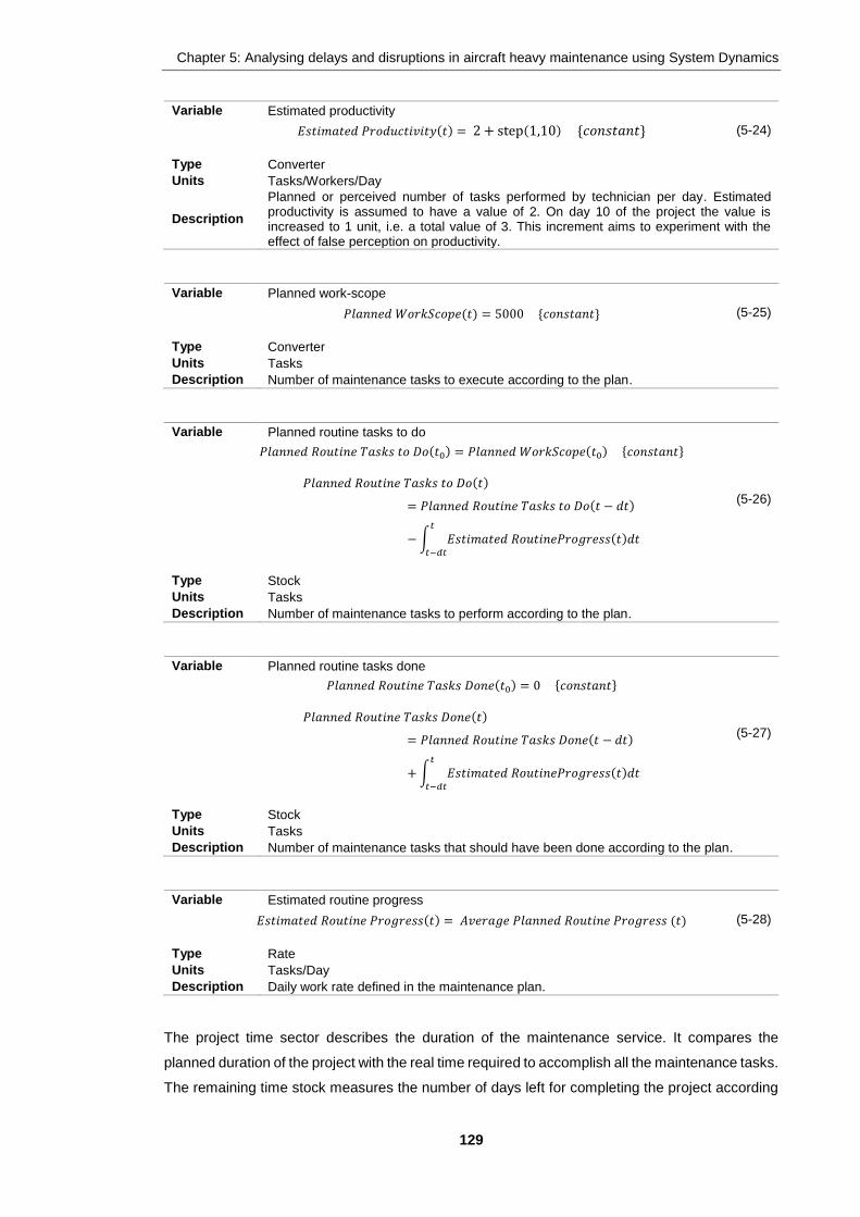
Chapter 5: Analysing delays and disruptions in aircraft heavy maintenance using System Dynamics
129
Variable Estimated productivity
𝐸𝑠𝑡𝑖𝑚𝑎𝑡𝑒𝑑 𝑃𝑟𝑜𝑑𝑢𝑐𝑡𝑖𝑣𝑖𝑡𝑦(𝑡) = 2 + step(1,10) {𝑐𝑜𝑛𝑠𝑡𝑎𝑛𝑡} (5-24)
Type Converter
Units Tasks/Workers/Day
Description
Planned or perceived number of tasks performed by technician per day. Estimated productivity is assumed to have a value of 2. On day 10 of the project the value is increased to 1 unit, i.e. a total value of 3. This increment aims to experiment with the effect of false perception on productivity.
Variable Planned work-scope
𝑃𝑙𝑎𝑛𝑛𝑒𝑑 𝑊𝑜𝑟𝑘𝑆𝑐𝑜𝑝𝑒(𝑡) = 5000 {𝑐𝑜𝑛𝑠𝑡𝑎𝑛𝑡} (5-25)
Type Converter
Units Tasks
Description Number of maintenance tasks to execute according to the plan.
Variable Planned routine tasks to do
𝑃𝑙𝑎𝑛𝑛𝑒𝑑 𝑅𝑜𝑢𝑡𝑖𝑛𝑒 𝑇𝑎𝑠𝑘𝑠 𝑡𝑜 𝐷𝑜(𝑡0) = 𝑃𝑙𝑎𝑛𝑛𝑒𝑑 𝑊𝑜𝑟𝑘𝑆𝑐𝑜𝑝𝑒(𝑡0) {𝑐𝑜𝑛𝑠𝑡𝑎𝑛𝑡}
𝑃𝑙𝑎𝑛𝑛𝑒𝑑 𝑅𝑜𝑢𝑡𝑖𝑛𝑒 𝑇𝑎𝑠𝑘𝑠 𝑡𝑜 𝐷𝑜(𝑡)
= 𝑃𝑙𝑎𝑛𝑛𝑒𝑑 𝑅𝑜𝑢𝑡𝑖𝑛𝑒 𝑇𝑎𝑠𝑘𝑠 𝑡𝑜 𝐷𝑜(𝑡 − 𝑑𝑡)
− ∫ 𝐸𝑠𝑡𝑖𝑚𝑎𝑡𝑒𝑑 𝑅𝑜𝑢𝑡𝑖𝑛𝑒𝑃𝑟𝑜𝑔𝑟𝑒𝑠𝑠(𝑡)𝑑𝑡𝑡
𝑡−𝑑𝑡
(5-26)
Type Stock
Units Tasks
Description Number of maintenance tasks to perform according to the plan.
Variable Planned routine tasks done
𝑃𝑙𝑎𝑛𝑛𝑒𝑑 𝑅𝑜𝑢𝑡𝑖𝑛𝑒 𝑇𝑎𝑠𝑘𝑠 𝐷𝑜𝑛𝑒(𝑡0) = 0 {𝑐𝑜𝑛𝑠𝑡𝑎𝑛𝑡}
𝑃𝑙𝑎𝑛𝑛𝑒𝑑 𝑅𝑜𝑢𝑡𝑖𝑛𝑒 𝑇𝑎𝑠𝑘𝑠 𝐷𝑜𝑛𝑒(𝑡)
= 𝑃𝑙𝑎𝑛𝑛𝑒𝑑 𝑅𝑜𝑢𝑡𝑖𝑛𝑒 𝑇𝑎𝑠𝑘𝑠 𝐷𝑜𝑛𝑒(𝑡 − 𝑑𝑡)
+ ∫ 𝐸𝑠𝑡𝑖𝑚𝑎𝑡𝑒𝑑 𝑅𝑜𝑢𝑡𝑖𝑛𝑒𝑃𝑟𝑜𝑔𝑟𝑒𝑠𝑠(𝑡)𝑑𝑡𝑡
𝑡−𝑑𝑡
(5-27)
Type Stock
Units Tasks
Description Number of maintenance tasks that should have been done according to the plan.
Variable Estimated routine progress
𝐸𝑠𝑡𝑖𝑚𝑎𝑡𝑒𝑑 𝑅𝑜𝑢𝑡𝑖𝑛𝑒 𝑃𝑟𝑜𝑔𝑟𝑒𝑠𝑠(𝑡) = 𝐴𝑣𝑒𝑟𝑎𝑔𝑒 𝑃𝑙𝑎𝑛𝑛𝑒𝑑 𝑅𝑜𝑢𝑡𝑖𝑛𝑒 𝑃𝑟𝑜𝑔𝑟𝑒𝑠𝑠 (𝑡) (5-28)
Type Rate
Units Tasks/Day
Description Daily work rate defined in the maintenance plan.
The project time sector describes the duration of the maintenance service. It compares the
planned duration of the project with the real time required to accomplish all the maintenance tasks.
The remaining time stock measures the number of days left for completing the project according

Chapter 5: Analysing delays and disruptions in aircraft heavy maintenance using System Dynamics
130
to the plan. By comparing the planned and real elapsed days, the total delay of the project can
be determined. Equations (5-29) to (5-36) present the characteristics of the variables of this
sector.
Variable Estimated project time
𝐸𝑠𝑡𝑖𝑚𝑎𝑡𝑒𝑑 𝑃𝑟𝑜𝑗𝑒𝑐𝑡 𝑇𝑖𝑚𝑒 = 50 {𝑐𝑜𝑛𝑠𝑡𝑎𝑛𝑡} (5-29)
Type Converter
Units Day (constant)
Description Total project time frame according to the maintenance plan.
Variable Percentage remaining time
𝑃𝑒𝑟𝑐𝑒𝑛𝑡𝑎𝑔𝑒 𝑅𝑒𝑚𝑎𝑖𝑛𝑖𝑛𝑔 𝑇𝑖𝑚𝑒(𝑡)
= 𝑅𝑒𝑚𝑎𝑖𝑛𝑖𝑛𝑔_𝑇𝑖𝑚𝑒(𝑡)/𝐸𝑠𝑡𝑖𝑚𝑎𝑡𝑒𝑑_𝑃𝑟𝑜𝑗𝑒𝑐𝑡_𝑇𝑖𝑚𝑒(𝑡) ∗ 100 (5-30)
Type Converter
Units Percentage
Description Remaining project time expressed as a percentage.
Variable Project delay
𝑃𝑟𝑜𝑗𝑒𝑐𝑡 𝑑𝑒𝑙𝑎𝑦(𝑡) = 𝑅𝑒𝑎𝑙__𝐸𝑙𝑎𝑝𝑠𝑒𝑑_𝑇𝑖𝑚𝑒(𝑡) − 𝑃𝑙𝑎𝑛𝑛𝑒𝑑_𝐸𝑙𝑎𝑝𝑠𝑒𝑑_𝑇𝑖𝑚𝑒(𝑡) (5-31)
Type Converter
Units Days
Description Project delay compared with the plan expressed in day.
Variable Planned elapsed time
𝑃𝑙𝑎𝑛𝑛𝑒𝑑 𝑒𝑙𝑎𝑝𝑠𝑒𝑑 𝑡𝑖𝑚𝑒(𝑡0) = 0 {𝑐𝑜𝑛𝑠𝑡𝑎𝑛𝑡}
𝑃𝑙𝑎𝑛𝑛𝑒𝑑 𝑒𝑙𝑎𝑝𝑠𝑒𝑑 𝑡𝑖𝑚𝑒(𝑡)
= 𝑃𝑙𝑎𝑛𝑛𝑒𝑑 𝑒𝑙𝑎𝑝𝑠𝑒𝑑 𝑡𝑖𝑚𝑒(𝑡 − 𝑑𝑡) + ∫ 𝑃𝑙𝑎𝑛𝑛𝑒𝑑 𝑡𝑖𝑚𝑒 𝑟𝑎𝑡𝑒(𝑡)𝑑𝑡𝑡
𝑡−𝑑𝑡
(5-32)
Type Stock
Units Days
Description Project elapsed days according to the plan.
Variable Real elapsed time
𝑅𝑒𝑎𝑙 𝑒𝑙𝑎𝑝𝑠𝑒𝑑 𝑡𝑖𝑚𝑒(𝑡0) = 0 {𝑐𝑜𝑛𝑠𝑡𝑎𝑛𝑡}
𝑅𝑒𝑎𝑙 𝑒𝑙𝑎𝑝𝑠𝑒𝑑 𝑡𝑖𝑚𝑒(𝑡) = 𝑅𝑒𝑎𝑙 𝑒𝑙𝑎𝑝𝑠𝑒𝑑 𝑡𝑖𝑚𝑒(𝑡 − 𝑑𝑡) + ∫ 𝑅𝑒𝑎𝑙 𝑡𝑖𝑚𝑒 𝑟𝑎𝑡𝑒(𝑡)𝑑𝑡𝑡
𝑡−𝑑𝑡
(5-33)
Type Stock
Units Days
Description Real elapsed days of the project.

Chapter 5: Analysing delays and disruptions in aircraft heavy maintenance using System Dynamics
131
Variable Remaining time
𝑅𝑒𝑚𝑎𝑖𝑛𝑖𝑛𝑔 𝑡𝑖𝑚𝑒(𝑡0) = 𝐸𝑠𝑡𝑖𝑚𝑎𝑡𝑒𝑑__𝑃𝑟𝑜𝑗𝑒𝑐𝑡_𝑇𝑖𝑚𝑒(𝑡) {𝑐𝑜𝑛𝑠𝑡𝑎𝑛𝑡}
𝑅𝑒𝑚𝑎𝑖𝑛𝑖𝑛𝑔 𝑡𝑖𝑚𝑒(𝑡) = 𝑅𝑒𝑚𝑎𝑖𝑛𝑖𝑛𝑔 𝑡𝑖𝑚𝑒(𝑡 − 𝑑𝑡) − ∫ 𝑃𝑙𝑎𝑛𝑛𝑒𝑑 𝑡𝑖𝑚𝑒 𝑟𝑎𝑡𝑒(𝑡)𝑑𝑡𝑡
𝑡−𝑑𝑡
(5-34)
Type Stock
Units Days
Description Days left to complete the project according to the plan.
Variable Planned time rate
𝑃𝑙𝑎𝑛𝑛𝑒𝑑 𝑡𝑖𝑚𝑒 𝑟𝑎𝑡𝑒(𝑡) = 𝑈𝑛𝑖𝑡 𝑇𝑖𝑚𝑒(𝑡) = 1 {𝐶𝑜𝑛𝑠𝑡𝑎𝑛𝑡} (5-35)
Type Rate
Units Days/Day
Description Counter of days.
Variable Real time rate
𝐼𝐹 𝑅𝑒𝑎𝑙_𝑅𝑜𝑢𝑡𝑖𝑛𝑒__𝑇𝑎𝑠𝑘𝑠_𝑡𝑜_𝐷𝑜 > 0
𝑇𝐻𝐸𝑁 𝑈𝑛𝑖𝑡 𝑇𝑖𝑚𝑒(𝑡) = 1 {𝐶𝑜𝑛𝑠𝑡𝑎𝑛𝑡}
𝐸𝐿𝑆𝐸 0 {𝐶𝑜𝑛𝑠𝑡𝑎𝑛𝑡}
(5-36)
Type Rate
Units Days/Day
Description Counter of days.
The real routine tasks sector depicts the execution of the maintenance project and the
adjustments made to meet the planned times, detailed in equations (5-37) to (5-47). The number
of scheduled tasks is defined in the real work-scope of the service. However, this figure is often
higher than the one defined in the plan, generating a backlog of activities since the beginning of
service that need to be corrected. The rate at which the routine tasks are performed is calculated
from the number of workers assigned to the process and their average productivity. During the
process, it is common to have a divergence between the real and reported number of tasks to be
done. This difference stems from the delay in reporting daily progress. A false perception of delay
may lead to assigning more resources than required. The backlog of tasks is determined by
comparing the planned against the real tasks to perform. If there is a backlog in the process, it is
frequently perceived belatedly. After the backlog of tasks has been recognised, there is also a
delay in adjusting the progress needed to meet the planned targets. The delays in recognising
the backlog of tasks and the adjustment in the pace of work vary depending on the stage of the
project. Typically, at the beginning of the project when there is no rush for completing on time, it
takes more time to recognise that adjustments in the process are required, but as the project
approaches its deadline and the pressure to finish on time increases, any required adjustment in
the process will be quickly identified. If the pace of work needs to be increased, more workers are
required, which leads the model to the workforce sector.

Chapter 5: Analysing delays and disruptions in aircraft heavy maintenance using System Dynamics
132
Variable Perceived backlog
𝑃𝑒𝑟𝑐𝑒𝑖𝑣𝑒𝑑 𝑏𝑎𝑐𝑘𝑙𝑜𝑔(𝑡)
= 𝑆𝑀𝑇𝐻1(𝑇𝑎𝑠𝑘𝑠_𝑡𝑜_𝐷𝑜_𝐵𝑎𝑐𝑘𝑙𝑜𝑔(𝑡), 𝑇𝑖𝑚𝑒_𝑡𝑜__𝑟𝑒𝑐𝑜𝑔𝑛𝑖𝑠𝑒__𝑡ℎ𝑒_𝐷𝑒𝑙𝑎𝑦(𝑡)) (5-37)
Type Converter
Units Tasks
Description Management perception regarding the project backlog of tasks. It uses a smoothing function (SMTH1) to model the delay in the variable.
Variable Productivity
𝑃𝑟𝑜𝑑𝑢𝑐𝑡𝑖𝑣𝑖𝑡𝑦(𝑡) = 2 {𝑐𝑜𝑛𝑠𝑡𝑎𝑛𝑡} (5-38)
Type Converter
Units Tasks/Workers/Day
Description Current average number of tasks performed by technician per day.
Variable Progress adjustment
𝑃𝑟𝑜𝑔𝑟𝑒𝑠𝑠 𝑎𝑑𝑗𝑢𝑠𝑡𝑚𝑒𝑛𝑡(𝑡) = 𝑃𝑒𝑟𝑐𝑒𝑖𝑣𝑒𝑑__𝐵𝑎𝑐𝑘𝑙𝑜𝑔(𝑡)/𝑇𝑖𝑚𝑒_𝑡𝑜__𝑎𝑑𝑗𝑢𝑠𝑡_𝑃𝑟𝑜𝑔𝑟𝑒𝑠𝑠(𝑡) (5-39)
Type Converter
Units Tasks/Day
Description Adjusted daily work rate required to meet the planned requirements.
Variable Progress needed
𝑃𝑟𝑜𝑔𝑟𝑒𝑠𝑠 𝑛𝑒𝑒𝑑𝑒𝑑(𝑡) =
𝐼𝐹, 𝑃𝑙𝑎𝑛𝑛𝑒𝑑_𝑅𝑜𝑢𝑡𝑖𝑛𝑒_𝑇𝑎𝑠𝑘𝑠_𝑡𝑜_𝐷𝑜(𝑡) > 0
𝑇𝐻𝐸𝑁, 𝐸𝑠𝑡𝑖𝑚𝑎𝑡𝑒𝑑__𝑅𝑜𝑢𝑡𝑖𝑛𝑒𝑃𝑟𝑜𝑔𝑟𝑒𝑠𝑠(𝑡) + 𝑃𝑟𝑜𝑔𝑟𝑒𝑠𝑠__𝐴𝑑𝑗𝑢𝑠𝑡𝑚𝑒𝑛𝑡(𝑡)
𝐸𝐿𝑆𝐸, 𝐴𝑣𝑒𝑟𝑎𝑔𝑒_𝑃𝑙𝑎𝑛𝑛𝑒𝑑__𝑅𝑜𝑢𝑡𝑖𝑛𝑒_𝑃𝑟𝑜𝑔𝑟𝑒𝑠𝑠(𝑡) + 𝑃𝑟𝑜𝑔𝑟𝑒𝑠𝑠__𝐴𝑑𝑗𝑢𝑠𝑡𝑚𝑒𝑛𝑡(𝑡)
(5-40)
Type Converter
Units Tasks/Day
Description Tasks per day that need to be done to complete the project according to the plan.
Variable Real work-scope
𝑅𝑒𝑎𝑙 𝑊𝑜𝑟𝑘 − 𝑆𝑐𝑜𝑝𝑒(𝑡) = 5000 {𝑐𝑜𝑛𝑠𝑡𝑎𝑛𝑡} (5-41)
Type Converter
Units Tasks
Description Real number of maintenance tasks to execute during the maintenance check.
Variable Reported tasks to do
𝑅𝑒𝑝𝑜𝑟𝑡𝑒𝑑 𝑡𝑎𝑠𝑘𝑠 𝑡𝑜 𝑑𝑜(𝑡)
= 𝐷𝑒𝑙𝑎𝑦(𝑅𝑒𝑎𝑙_𝑅𝑜𝑢𝑡𝑖𝑛𝑒__𝑇𝑎𝑠𝑘𝑠_𝑡𝑜_𝐷𝑜(𝑡), 𝑇𝑖𝑚𝑒_𝑡𝑜_𝑟𝑒𝑝𝑜𝑟𝑡__𝑅𝑒𝑎𝑙_𝑃𝑟𝑜𝑔𝑟𝑒𝑠𝑠(𝑡)) (5-42)
Type Converter
Units Tasks
Description The registered number of tasks to do.

Chapter 5: Analysing delays and disruptions in aircraft heavy maintenance using System Dynamics
133
Variable Tasks to do backlog
𝑇𝑎𝑠𝑘𝑠 𝑡𝑜 𝑑𝑜 𝑏𝑎𝑐𝑘𝑙𝑜𝑔(𝑡)
= 𝑅𝑒𝑎𝑙_𝑅𝑜𝑢𝑡𝑖𝑛𝑒_𝑇𝑎𝑠𝑘𝑠 𝑡𝑜 𝐷𝑜(𝑡)
− 𝑃𝑙𝑎𝑛𝑛𝑒𝑑_𝑅𝑜𝑢𝑡𝑖𝑛𝑒_𝑇𝑎𝑠𝑘𝑠_𝑡𝑜_𝐷𝑜(𝑡)
(5-43)
Type Converter
Units Tasks
Description Accumulation of uncompleted tasks compared with that planned tasks that should have been done.
Variable Time to report real progress
𝑇𝑖𝑚𝑒 𝑡𝑜 𝑟𝑒𝑝𝑜𝑟𝑡 𝑟𝑒𝑎𝑙 𝑝𝑟𝑜𝑔𝑟𝑒𝑠𝑠(𝑡) = 1 {𝑐𝑜𝑛𝑠𝑡𝑎𝑛𝑡} (5-44)
Type Converter
Units Days
Description Delay in registering and reporting the real progress.
Variable Time to adjust progress
𝑇𝑖𝑚𝑒 𝑡𝑜 𝑎𝑑𝑗𝑢𝑠𝑡 𝑝𝑟𝑜𝑔𝑟𝑒𝑠𝑠(𝑡) = 𝑓(𝑃𝑒𝑟𝑐𝑒𝑛𝑡𝑎𝑔𝑒 𝑅𝑒𝑚𝑎𝑖𝑛𝑖𝑛𝑔 𝑇𝑖𝑚𝑒(𝑡)) (5-45)
Type Converter
Units Days
Description Delay to acknowledge the real progress. Represents a variable delay according to the project progress and is defined by a graphical function that relates the delay with the remaining time of the project.
Variable Time to recognise the delay
𝑇𝑖𝑚𝑒 𝑡𝑜 𝑟𝑒𝑐𝑜𝑔𝑛𝑖𝑠𝑒 𝑡ℎ𝑒 𝑑𝑒𝑙𝑎𝑦 (𝑡) = 𝑓(𝑃𝑒𝑟𝑐𝑒𝑛𝑡𝑎𝑔𝑒 𝑅𝑒𝑚𝑎𝑖𝑛𝑖𝑛𝑔 𝑇𝑖𝑚𝑒(𝑡)) (5-46)
Type Converter
Units Days
Description Delay to acknowledge the backlog of tasks. Represents a variable delay according to the project progress and is defined by a graphical function that relates the delay with the remaining time of the project.
Variable Real routine progress
𝑅𝑒𝑎𝑙 𝑟𝑜𝑢𝑡𝑖𝑛𝑒 𝑝𝑟𝑜𝑔𝑟𝑒𝑠𝑠(𝑡) = 𝑊𝑜𝑟𝑘𝑓𝑜𝑟𝑐𝑒__𝐴𝑠𝑠𝑖𝑔𝑛𝑒𝑑(𝑡) ∗ 𝑃𝑟𝑜𝑑𝑢𝑐𝑡𝑖𝑣𝑖𝑡𝑦(𝑡) (5-47)
Type Rate
Units Tasks/Day
Description Number of tasks executed by day.
Variable Real routine tasks to do
𝑅𝑒𝑎𝑙 𝑟𝑜𝑢𝑡𝑖𝑛𝑒 𝑡𝑎𝑠𝑘𝑠 𝑡𝑜 𝑑𝑜(𝑡0) = 𝑅𝑒𝑎𝑙 𝑊𝑜𝑟𝑘𝑆𝑐𝑜𝑝𝑒(𝑡) {𝑐𝑜𝑛𝑠𝑡𝑎𝑛𝑡}
𝑅𝑒𝑎𝑙 𝑟𝑜𝑢𝑡𝑖𝑛𝑒 𝑡𝑎𝑠𝑘𝑠 𝑡𝑜 𝑑𝑜(𝑡)
= 𝑅𝑒𝑎𝑙 𝑟𝑜𝑢𝑡𝑖𝑛𝑒 𝑡𝑎𝑠𝑘𝑠 𝑡𝑜 𝑑𝑜(𝑡 − 𝑑𝑡)
− ∫ 𝑅𝑒𝑎𝑙 𝑅𝑜𝑢𝑡𝑖𝑛𝑒 𝑃𝑟𝑜𝑔𝑟𝑒𝑠𝑠(𝑡)𝑑𝑡𝑡
𝑡−𝑑𝑡
(5-48)
Type Stock
Units Tasks
Description Number of maintenance tasks to perform.

Chapter 5: Analysing delays and disruptions in aircraft heavy maintenance using System Dynamics
134
Variable Real routine tasks done
𝑅𝑒𝑎𝑙 𝑟𝑜𝑢𝑡𝑖𝑛𝑒 𝑡𝑎𝑠𝑘𝑠 𝑑𝑜𝑛𝑒(𝑡0) = 𝑅𝑒𝑎𝑙 𝑊𝑜𝑟𝑘𝑆𝑐𝑜𝑝𝑒(𝑡) {𝑐𝑜𝑛𝑠𝑡𝑎𝑛𝑡}
𝑅𝑒𝑎𝑙 𝑟𝑜𝑢𝑡𝑖𝑛𝑒 𝑡𝑎𝑠𝑘𝑠 𝑑𝑜𝑛𝑒(𝑡)
= 𝑅𝑒𝑎𝑙 𝑟𝑜𝑢𝑡𝑖𝑛𝑒 𝑡𝑎𝑠𝑘𝑠 𝑑𝑜𝑛𝑒(𝑡 − 𝑑𝑡)
+ ∫ 𝑅𝑒𝑎𝑙 𝑅𝑜𝑢𝑡𝑖𝑛𝑒 𝑃𝑟𝑜𝑔𝑟𝑒𝑠𝑠(𝑡)𝑑𝑡𝑡
𝑡−𝑑𝑡
(5-49)
Type Stock
Units Tasks
Description Number of maintenance tasks already executed.
The workforce sector describes the allocation of labour to execute maintenance tasks. Once the
necessity of increasing the progress rate has been recognised, the requirement is translated into
the need to increase workforce assigned to the execution of the maintenance tasks. However,
the additional workforce requirement is inaccurately informed by perceived rather than real
process productivity and there is also a delay in recognising the adjustment in the workforce.
Allocating available technicians to the process requires time and is subject to the attitude of the
management towards increasing the workforce assigned to the process. This attitude tends to
vary depending on the status of the maintenance check. At the early stages of the project or if the
perception of delay is weak, there is a reluctance to assign more resources and a lower
percentage is allocated than required, but at the end of the service when the pressure to finish on
time increases, management is willing to assign even more resources than originally requested.
When more technicians are allocated to perform maintenance tasks, the progress rate increases
and the balancing loop is closed.
If the available headcount is insufficient to cope with the demand to allocate more technicians to
the process, the pressure to expand the roster increases. However, this requirement is also
affected by the attitudes and perceptions of the management. Generally, the administration is
slow to accept that it is necessary to adjust the number of available workers and is resistant to
the idea of augmenting the headcount. Once the decision to increase the available workforce has
been made either by withdrawing personnel from other processes or by hiring new ones, it will
take time to take effect due to the specialised nature of these resources. A detailed description of
the variables considered within this sector is included in equations (5-51) to (5-65).
Variable Initial workforce available
𝐼𝑛𝑖𝑡𝑖𝑎𝑙 𝑤𝑜𝑟𝑘𝑓𝑜𝑟𝑐𝑒 𝑎𝑣𝑎𝑖𝑙𝑎𝑏𝑙𝑒(𝑡) = 50 {𝑐𝑜𝑛𝑠𝑡𝑎𝑛𝑡} (5-50)
Type Converter
Units Workers
Description Headcount available at the beginning of the project.

Chapter 5: Analysing delays and disruptions in aircraft heavy maintenance using System Dynamics
135
Variable Additional workforce required
𝐴𝑑𝑑𝑖𝑡𝑖𝑜𝑛𝑎𝑙 𝑤𝑜𝑟𝑘𝑓𝑜𝑟𝑐𝑒 𝑟𝑒𝑞𝑢𝑖𝑟𝑒𝑑(𝑡) =
𝐼𝐹 𝑊𝑜𝑟𝑘𝑓𝑜𝑟𝑐𝑒𝑛𝑒𝑒𝑑𝑒𝑑(𝑡) > (𝑊𝑜𝑟𝑘𝑓𝑜𝑟𝑐𝑒𝐴𝑣𝑎𝑖𝑙𝑎𝑏𝑙𝑒(𝑡) + 𝑊𝑜𝑟𝑘𝑓𝑜𝑟𝑐𝑒𝐴𝑠𝑠𝑖𝑔𝑛𝑒𝑑(𝑡))
𝑇𝐻𝐸𝑁 𝑊𝑜𝑟𝑘𝑓𝑜𝑟𝑐𝑒𝑛𝑒𝑒𝑑𝑒𝑑(𝑡) − (𝑊𝑜𝑟𝑘𝑓𝑜𝑟𝑐𝑒𝐴𝑣𝑎𝑖𝑙𝑎𝑏𝑙𝑒(𝑡) + 𝑊𝑜𝑟𝑘𝑓𝑜𝑟𝑐𝑒𝐴𝑠𝑠𝑖𝑔𝑛𝑒𝑑(𝑡)) , 𝐸𝐿𝑆𝐸 0
(5-51)
Type Converter
Units Workers
Description Additional workers needed to cope with the demand of work.
Variable Initial workforce assigned
𝐼𝑛𝑖𝑡𝑖𝑎𝑙 𝑤𝑜𝑟𝑘𝑓𝑜𝑟𝑐𝑒 𝑎𝑠𝑠𝑖𝑔𝑛𝑒𝑑(𝑡)
= 𝐴𝑣𝑒𝑟𝑎𝑔𝑒_𝑃𝑙𝑎𝑛𝑛𝑒𝑑__𝑅𝑜𝑢𝑡𝑖𝑛𝑒_𝑃𝑟𝑜𝑔𝑟𝑒𝑠𝑠(𝑡)
/𝐸𝑠𝑡𝑖𝑚𝑎𝑡𝑒𝑑__𝑃𝑟𝑜𝑑𝑢𝑐𝑡𝑖𝑣𝑖𝑡𝑦(𝑡)
(5-52)
Type Converter
Units Workers
Description Workers assigned to perform routines tasks at the beginning of the service.
Variable Management attitude towards increasing workforce
𝑀𝑎𝑛𝑎𝑔𝑒𝑚𝑒𝑛𝑡 𝑎𝑡𝑡𝑖𝑡𝑢𝑑𝑒 𝑡𝑜𝑤𝑎𝑟𝑑𝑠 𝑖𝑛𝑐𝑟𝑒𝑎𝑠𝑖𝑛𝑔 𝑤𝑜𝑟𝑘𝑓𝑜𝑟𝑐𝑒(𝑡): 𝑉𝑎𝑙𝑢𝑒𝑠 𝑓𝑟𝑜𝑚 0.5 𝑡𝑜 1.5 {𝑟𝑎𝑛𝑔𝑒} (5-53)
Type Converter
Units Proportion
Description Stance towards augmenting the headcount.
Variable Management bias
𝑀𝑎𝑛𝑎𝑔𝑒𝑚𝑒𝑛𝑡 𝑏𝑖𝑎𝑠: 𝑉𝑎𝑙𝑢𝑒𝑠 𝑓𝑟𝑜𝑚 0.5 𝑡𝑜 1.5 {𝑟𝑎𝑛𝑔𝑒} (5-54)
Type Converter
Units Proportion
Description Stance towards allocating more labour to execute routine tasks.
Variable Perceived additional workforce required
𝑃𝑒𝑟𝑐𝑒𝑖𝑣𝑒𝑑 𝑎𝑑𝑑𝑖𝑡𝑖𝑜𝑛𝑎𝑙 𝑤𝑜𝑟𝑘𝑓𝑜𝑟𝑐𝑒 𝑟𝑒𝑞𝑢𝑖𝑟𝑒𝑑(𝑡)
= 𝑆𝑀𝑇𝐻1(𝐴𝑑𝑑𝑖𝑡𝑖𝑜𝑛𝑎𝑙__𝑊𝑜𝑟𝑘𝑓𝑜𝑟𝑐𝑒_𝑟𝑒𝑞𝑢𝑖𝑟𝑒𝑑(𝑡)
∗ 𝑀𝑔𝑚𝑡_𝐴𝑡𝑡𝑖𝑡𝑢𝑑𝑒_𝑡𝑜𝑤𝑎𝑟𝑑𝑠_𝑖𝑛𝑐𝑟𝑒𝑎𝑠𝑖𝑛𝑔_𝑤𝑜𝑟𝑘𝑓𝑜𝑟𝑐𝑒(𝑡), 𝑇𝑖𝑚𝑒_𝑡𝑜𝑅𝑒𝑐𝑜𝑔𝑛𝑖𝑠𝑒_𝑎𝑑𝑑_𝑤𝑜𝑟𝑘𝑓𝑜𝑟𝑐𝑒(𝑡)
(5-55)
Type Converter
Units Workers
Description Perception regarding the additional workers needed to cope with the demand of work.
Variable Time to increase the workforce
𝑇𝑖𝑚𝑒 𝑡𝑜 𝑖𝑛𝑐𝑟𝑒𝑎𝑠𝑒 𝑡ℎ𝑒 𝑤𝑜𝑟𝑘𝑓𝑜𝑟𝑐𝑒(𝑡) = 5 {𝑐𝑜𝑛𝑠𝑡𝑎𝑛𝑡} (5-56)
Type Converter
Units Days
Description Delay in increasing the available workforce.

Chapter 5: Analysing delays and disruptions in aircraft heavy maintenance using System Dynamics
136
Variable Time to recognise additional workforce
𝑇𝑖𝑚𝑒 𝑡𝑜 𝑟𝑒𝑐𝑜𝑔𝑛𝑖𝑠𝑒 𝑎𝑑𝑑𝑖𝑡𝑖𝑜𝑛𝑎𝑙 𝑤𝑜𝑟𝑘𝑓𝑜𝑟𝑐𝑒(𝑡) = 2 {𝑐𝑜𝑛𝑠𝑡𝑎𝑛𝑡} (5-57)
Type Converter
Units Days
Description Delay in accepting that more resources are required.
Variable Time to adjust workforce
𝑇𝑖𝑚𝑒 𝑡𝑜 𝑎𝑑𝑗𝑢𝑠𝑡 𝑤𝑜𝑟𝑘𝑓𝑜𝑟𝑐𝑒(𝑡) {𝑐𝑜𝑛𝑠𝑡𝑎𝑛𝑡} (5-58)
Type Converter
Units Days
Description Delay in acknowledging that more technicians need to be assigned to routines.
Variable Workforce adjustment
𝑊𝑜𝑟𝑘𝑓𝑜𝑟𝑐𝑒 𝑎𝑑𝑗𝑢𝑠𝑡𝑚𝑒𝑛𝑡(𝑡)
= ((𝑊𝑜𝑟𝑘𝑓𝑜𝑟𝑐𝑒__𝑛𝑒𝑒𝑑𝑒𝑑(𝑡)
− 𝑊𝑜𝑟𝑘𝑓𝑜𝑟𝑐𝑒__𝐴𝑠𝑠𝑖𝑔𝑛𝑒𝑑(𝑡))/𝑇𝑖𝑚𝑒_𝑡𝑜__𝑎𝑑𝑗𝑢𝑠𝑡_𝑊𝑜𝑟𝑘𝑓𝑜𝑟𝑐𝑒(𝑡))
∗ 𝑀𝑎𝑛𝑎𝑔𝑒𝑚𝑒𝑛𝑡_𝐵𝑖𝑎𝑠(𝑡)
(5-59)
Type Converter
Units Workers/Day
Description Adapts the resource allocation according to the project status.
Variable Workforce needed
𝑊𝑜𝑟𝑘𝑓𝑜𝑟𝑐𝑒 𝑛𝑒𝑒𝑑𝑒𝑑(𝑡)
= 𝑆𝑀𝑇𝐻1(𝑃𝑟𝑜𝑔𝑟𝑒𝑠𝑠__𝑛𝑒𝑒𝑑𝑒𝑑(𝑡)
/𝐸𝑠𝑡𝑖𝑚𝑎𝑡𝑒𝑑__𝑃𝑟𝑜𝑑𝑢𝑐𝑡𝑖𝑣𝑖𝑡𝑦(𝑡), 𝑊𝑜𝑟𝑘𝑓𝑜𝑟𝑐𝑒__𝑃𝑙𝑎𝑛𝑛𝑖𝑛𝑔_𝐷𝑒𝑙𝑎𝑦(𝑡))
(5-60)
Type Converter
Units Workers
Description The number of workers required to meet the project goals.
Variable Workforce planning delay
𝑊𝑜𝑟𝑘𝑓𝑜𝑟𝑐𝑒 𝑝𝑙𝑎𝑛𝑛𝑖𝑛𝑔 𝑑𝑒𝑙𝑎𝑦(𝑡) {𝑐𝑜𝑛𝑠𝑡𝑎𝑛𝑡} (5-61)
Type Converter
Units Days
Description Delay in recognising the requirement of personnel.
Variable Workforce assigned
𝑊𝑜𝑟𝑘𝑓𝑜𝑟𝑐𝑒 𝑎𝑠𝑠𝑖𝑔𝑛𝑒𝑑(𝑡0) = 𝐼𝑛𝑖𝑡𝑖𝑎𝑙 𝑊𝑜𝑟𝑘𝑓𝑜𝑟𝑐𝑒 𝑎𝑠𝑠𝑖𝑔𝑛𝑒𝑑(𝑡) {𝑐𝑜𝑛𝑠𝑡𝑎𝑛𝑡}
𝑊𝑜𝑟𝑘𝑓𝑜𝑟𝑐𝑒 𝑎𝑠𝑠𝑖𝑔𝑛𝑒𝑑(𝑡)
= 𝑊𝑜𝑟𝑘𝑓𝑜𝑟𝑐𝑒 𝑎𝑠𝑠𝑖𝑔𝑛𝑒𝑑(𝑡 − 𝑑𝑡) ± ∫ 𝐴𝑙𝑙𝑜𝑐𝑎𝑡𝑖𝑜𝑛 𝑅𝑎𝑡𝑒(𝑡)𝑑𝑡𝑡
𝑡−𝑑𝑡
(5-62)
Type Stock
Units Workers
Description Number of workers allocated to execute the maintenance tasks.
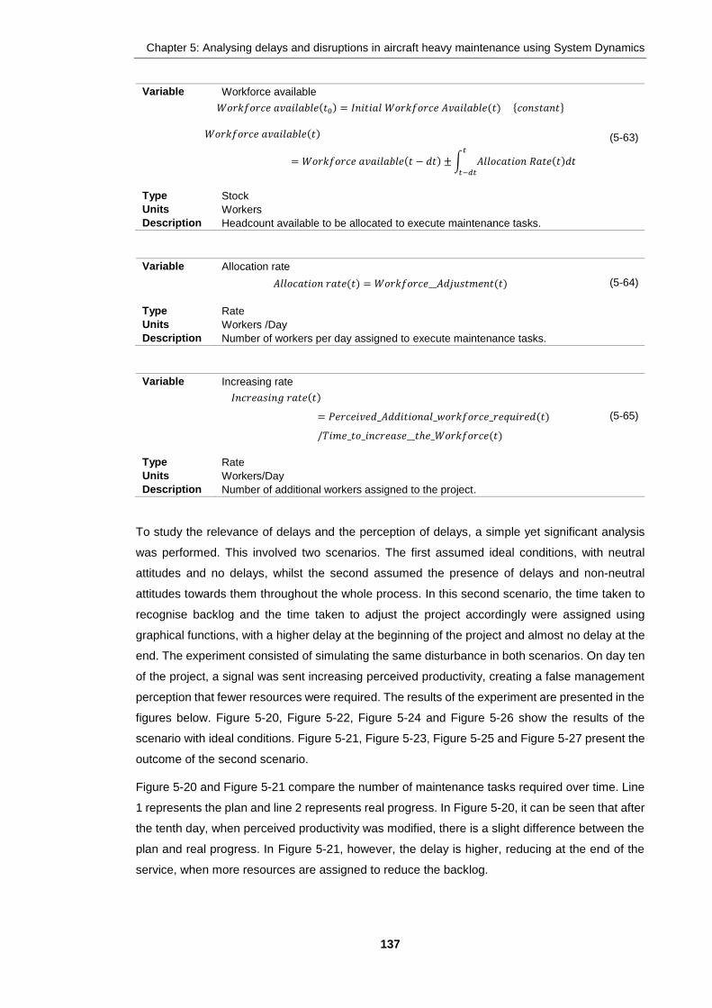
Chapter 5: Analysing delays and disruptions in aircraft heavy maintenance using System Dynamics
137
Variable Workforce available
𝑊𝑜𝑟𝑘𝑓𝑜𝑟𝑐𝑒 𝑎𝑣𝑎𝑖𝑙𝑎𝑏𝑙𝑒(𝑡0) = 𝐼𝑛𝑖𝑡𝑖𝑎𝑙 𝑊𝑜𝑟𝑘𝑓𝑜𝑟𝑐𝑒 𝐴𝑣𝑎𝑖𝑙𝑎𝑏𝑙𝑒(𝑡) {𝑐𝑜𝑛𝑠𝑡𝑎𝑛𝑡}
𝑊𝑜𝑟𝑘𝑓𝑜𝑟𝑐𝑒 𝑎𝑣𝑎𝑖𝑙𝑎𝑏𝑙𝑒(𝑡)
= 𝑊𝑜𝑟𝑘𝑓𝑜𝑟𝑐𝑒 𝑎𝑣𝑎𝑖𝑙𝑎𝑏𝑙𝑒(𝑡 − 𝑑𝑡) ± ∫ 𝐴𝑙𝑙𝑜𝑐𝑎𝑡𝑖𝑜𝑛 𝑅𝑎𝑡𝑒(𝑡)𝑑𝑡𝑡
𝑡−𝑑𝑡
(5-63)
Type Stock
Units Workers
Description Headcount available to be allocated to execute maintenance tasks.
Variable Allocation rate
𝐴𝑙𝑙𝑜𝑐𝑎𝑡𝑖𝑜𝑛 𝑟𝑎𝑡𝑒(𝑡) = 𝑊𝑜𝑟𝑘𝑓𝑜𝑟𝑐𝑒__𝐴𝑑𝑗𝑢𝑠𝑡𝑚𝑒𝑛𝑡(𝑡) (5-64)
Type Rate
Units Workers /Day
Description Number of workers per day assigned to execute maintenance tasks.
Variable Increasing rate
𝐼𝑛𝑐𝑟𝑒𝑎𝑠𝑖𝑛𝑔 𝑟𝑎𝑡𝑒(𝑡)
= 𝑃𝑒𝑟𝑐𝑒𝑖𝑣𝑒𝑑_𝐴𝑑𝑑𝑖𝑡𝑖𝑜𝑛𝑎𝑙_𝑤𝑜𝑟𝑘𝑓𝑜𝑟𝑐𝑒_𝑟𝑒𝑞𝑢𝑖𝑟𝑒𝑑(𝑡)
/𝑇𝑖𝑚𝑒_𝑡𝑜_𝑖𝑛𝑐𝑟𝑒𝑎𝑠𝑒__𝑡ℎ𝑒_𝑊𝑜𝑟𝑘𝑓𝑜𝑟𝑐𝑒(𝑡)
(5-65)
Type Rate
Units Workers/Day
Description Number of additional workers assigned to the project.
To study the relevance of delays and the perception of delays, a simple yet significant analysis
was performed. This involved two scenarios. The first assumed ideal conditions, with neutral
attitudes and no delays, whilst the second assumed the presence of delays and non-neutral
attitudes towards them throughout the whole process. In this second scenario, the time taken to
recognise backlog and the time taken to adjust the project accordingly were assigned using
graphical functions, with a higher delay at the beginning of the project and almost no delay at the
end. The experiment consisted of simulating the same disturbance in both scenarios. On day ten
of the project, a signal was sent increasing perceived productivity, creating a false management
perception that fewer resources were required. The results of the experiment are presented in the
figures below. Figure 5-20, Figure 5-22, Figure 5-24 and Figure 5-26 show the results of the
scenario with ideal conditions. Figure 5-21, Figure 5-23, Figure 5-25 and Figure 5-27 present the
outcome of the second scenario.
Figure 5-20 and Figure 5-21 compare the number of maintenance tasks required over time. Line
1 represents the plan and line 2 represents real progress. In Figure 5-20, it can be seen that after
the tenth day, when perceived productivity was modified, there is a slight difference between the
plan and real progress. In Figure 5-21, however, the delay is higher, reducing at the end of the
service, when more resources are assigned to reduce the backlog.

Chapter 5: Analysing delays and disruptions in aircraft heavy maintenance using System Dynamics
138
Figure 5-20 Remaining number of tasks per day (ideal conditions)
Figure 5-21 Remaining number of tasks per day (with delays)
Figure 5-22 and Figure 5-23 portray the change in productivity and how workforce allocation is
affected by this perception. Line 1 represents estimated productivity, line 2 the workforce needed
to meet the deadlines and line 3 the workforce that is assigned to execute maintenance tasks.
Line 4 shows the real work progress. In Figure 5-22, it can be seen that after perceived
productivity is adjusted, less workforce is required and consequently the level of workforce
allocated to the process falls. However, as productivity has not actually changed, real progress
also drops, sending a signal to adjust the workforce. Due to there being no delays in this scenario,
the system is adjusted almost immediately and is operating as under the initial conditions after a
couple of days. Figure 5-23 presents different behaviour. Here, when productivity is increased,
there is a delay in perceiving that less workforce is needed and real progress gradually decreases.
By the time the system has identified the false perception, the backlog of tasks is already
significant. More resources are assigned to the process but because of the delay, the re-allocation

Chapter 5: Analysing delays and disruptions in aircraft heavy maintenance using System Dynamics
139
of personnel takes time. By the end of the service, in an attempt to overcome this issue, a large
volume of resources is assigned.
Figure 5-24 to Figure 5-27 depict the backlog of tasks and also show the relationship backlog has
with the additional headcount required to meet work demand. In the first scenario (Figure 5-24
and Figure 5-26), the backlog remains almost without variation after the change in perceived
productivity and the system itself regulates the workforce needed. In contrast, there is more
fluctuation in the variables in the second scenario, shown in Figure 5-25 and Figure 5-27. Due to
delays in the process, the backlog increases considerably and a point is reached where this
cannot be corrected with the resources available. It then becomes necessary to increase the
headcount.
Figure 5-22 Workforce allocation per day (ideal conditions)
Figure 5-23 Workforce allocation per day (with delays)

Chapter 5: Analysing delays and disruptions in aircraft heavy maintenance using System Dynamics
140
Figure 5-24 Project backlog (ideal conditions)
Figure 5-25 Project backlog (with delays)
Figure 5-26 Additional workforce required (ideal conditions)

Chapter 5: Analysing delays and disruptions in aircraft heavy maintenance using System Dynamics
141
Figure 5-27 Additional workforce required (with delays)
This simple example shows how a slight change in the system has a significant impact, especially
if the information does not flow properly in the system or if the decision makers take an incorrect
approach.
5.4 Model validation
As previously discussed, validation in SD may be very difficult and subjective. The validation of
the developed SD models was performed in several stages throughout the modelling process
rather than as a single and isolated step. Firstly, through various feedback meetings, the
coherence and structure of the conceptual model was reviewed and discussed with different
experts in the industry to ensure that the problem was represented as accurately as possible.
Secondly, for the quantitative models, the consistency of the mathematical equations was revised
and a dimensional analysis was performed to verify that they were coherent in characterising the
problem. Finally, several simulation scenarios were run to assess the general behaviour of the
model and to identify unexpected results.
A natural step in the validation process would be to perform rigorous analytical tests to evaluate
the effectiveness of the model in describing the real behaviour of the system. However, due to
the sensitivity of the information it was difficult to gather enough data about the performance of
process to conduct these analytical tests. Therefore, it was necessary to perform a validation of
the model behaviour based on experts’ experience regarding the observed behaviour of the
maintenance process. For this, the quantitative models were discussed with experts who were
then allowed to experiment by changing the values of certain variables related to particular
maintenance strategies. Through developing and running different scenarios, the behaviour of
the model was compared with the results they expected according to their experience.
In general, the experts were satisfied with the overall behaviour of the model, pointing out that the
results obtained throughout the several scenarios were remarkably similar to the results they have
encountered in real life, particularly when experimenting with the effects of non-routine rate and
discovery rate on project duration. They also showed interest in the influence that management
Chapter 5: Analysing delays and disruptions in aircraft heavy maintenance using System Dynamics
142
perceptions and attitudes have on project performance, agreeing that these are problems
commonly faced during the execution of a maintenance check.
Notwithstanding the satisfactory results of the models, the experts raised serious concerns
regarding their possible applicability. They noted that the models are very simple and do not take
into account other relevant process factors, such as the skill of the personnel (which may affect
the type of tasks they can perform), the number of inspectors available during the process
(important as they find and evaluate non-routine tasks), or the availability of spare parts and tools,
which may also affect the execution of the maintenance check. Additionally, they pointed out that
the models make disputable assumptions that are seldom seen in real life, such as assuming
constant personnel productivity and an average duration for tasks.
In general terms, the experts concluded that the models could be useful for gaining insight into
the main challenges faced during heavy maintenance and as a learning instrument to explore the
effects of particular maintenance strategies. However, they were not totally convinced that at this
stage the models can be used to estimate the outcome of a maintenance service and therefore
be used as a decision support tool.
5.5 Summary
In this chapter, the SD methodology was used to develop a qualitative model and two quantitative
models aiming to analyse the delays and disruptions that occur during the execution of aircraft
heavy maintenance services. The conceptual model was used to portray the feedback structure
of the system and to analyse the complex interrelation between scheduled and unscheduled
tasks. The quantitative models were used to describe particular aspects of the problem and to
explore their effects on the duration of the maintenance service.
The conceptual model was developed based on experience and further enhanced through an
iterative process with the help of experts in the field. In summary, this model describes how
resources are allocated to perform scheduled tasks according to the plan and whether it is
necessary to reduce any backlog of tasks. However, during the execution of routine tasks,
unexpected damage, failures and discrepancies are discovered that require the programming of
unscheduled tasks to correct them. The stochastic nature of unscheduled activities hinders the
planning and control of tasks and resources. The main problem arises when available resources
must be distributed and allocated between scheduled and unscheduled tasks, causing delays and
disruptions during the process which might force a request for additional resources or an
extension of the aeroplane delivery date.
The causal loop diagrams proved to be a highly useful tool to improve not only the understanding
of the problem but also offer a wider vision of the process. They depict cause-and-effect
relationships between variables and feedback loops in the system and illuminate the complex
interactions between routine and non-routine tasks that hinder the management of resources and
the control of the whole maintenance service. The conceptual model illustrates that although the
uncertainty in the occurrence of unscheduled maintenance tasks is external to the process, the

Chapter 5: Analysing delays and disruptions in aircraft heavy maintenance using System Dynamics
143
management of the process and the complex interaction between the elements in the system
exacerbates the problem and causes delays and disruptions during the process. During the
development of the conceptual model in the feedback meetings, the causal loop diagrams proved
to be very valuable for facilitating communication and for promoting learning and discussion.
Despite the valuable findings obtained, the conceptual model does not have the ability to describe
the dynamic behaviour of the system. For this reason, two quantitative models were developed
using stock and flow diagrams. The first model analyses the effect of the arising of non-routines
and the distribution of workforce between scheduled and non-scheduled tasks. Through
simulation, three main issues were found. Firstly, after exploring the relation between the non-
routine rate and the workload of the maintenance project and the allocation of the available
resources, it was found that determining an accurate non-routine rate is essential to avoid
shortage or excess of resources. Secondly, it was found that there is a direct relationship between
discovery rate and the duration of the project, where an early discovery of discrepancies may
increase the chances of completing the project on time. Finally, different distributions of workforce
were explored to assess their impact on the service duration, demonstrating that a variable
allocation is the most suitable strategy for reducing the project time.
The second model explores the effect that managers’ perceptions have on the project
performance. This model shows that even without the uncertainty factor, managerial attitudes
towards delays have a significant impact on the decision-making process. It was shown that
delays cause false perceptions about the real status of the project and make misguided decisions
more likely. Delays are regulated by the speed at which information flows, and the sooner the
information is updated, the less impact delays will have on overall performance. Attitudes are
influenced by perception of project performance and the stage of execution and can aggravate
fluctuations in the system, interfering with resource management.
The quantitative models helped to gain awareness of the complex interactions between the
variables involved during aircraft maintenance and allowed experimentation with the dynamic
behaviour of the system. Through the definition and comparison of different scenarios, it was
possible to determine the relevance of certain variables for project performance, for instance the
importance of using more rigorous methods to determine the non-routine rate and to decide
optimal workforce allocation between the two types of maintenance task.

144
Chapter 6: Estimation of unscheduled
maintenance tasks using the Evidential
Reasoning rule
Uncertainty is inherent in almost any project and complex system and aircraft maintenance is no
exception. Unscheduled maintenance tasks arise from unexpected damage, failures and
discrepancies that are usually discovered during inspections performed as part of scheduled
maintenance checks. The uncertainty triggered by the stochastic nature of these unforeseen
events hinders the planning of non-routine tasks and the estimation and allocation of the
resources required to accomplish them. As a consequence, managing these additional
maintenance tasks is critical, as they might affect the cost, duration and quality of maintenance
checks.
Usually, before starting a heavy maintenance check, the number of routine tasks to perform is
well known, since they are clearly defined in the maintenance scheduled programme. In contrast,
even when the occurrence of unscheduled activities is considered, the number of non-routine
tasks is unknown before commencing the service. The exact number of unscheduled tasks is only
determined once the maintenance check has been completed.
The number of non-routine tasks may vary from one service to another. It is highly related to the
amount of damage and the number of failures, which depend on different factors such as
environmental conditions, the utilisation and the age of the aircraft and the quality of previous
maintenance checks, amongst others. Therefore, it is difficult to determine the total number of
non-routine tasks in advance. Besides, this figure by itself does not represent the actual impact
that additional unplanned activities have on the maintenance check as a whole, and also
complicates comparison between different services. Consequently, it is proposed to use the non-
routine rate as an indicator of the number of unplanned activities expressed as the ratio between
the number of unscheduled and scheduled activities.
In this chapter, a novel approach is proposed to estimate unplanned maintenance activities by
developing a model based on the evidential reasoning rule. The proposed model allows for more
precise estimation of non-routine rate for a specific heavy maintenance check by analysing
historical data relating to the usage and maintenance of an aeroplane. This approach attempts to
analyse from a different perspective the uncertainty of unforeseen events that can cause delays
in and disruption to complex projects.
The chapter has been organised in the following way. Firstly, the data and the variables used for
building the model are described. Secondly, a brief statistical analysis is performed to better
understand the variables and their interrelationships. Thirdly, to facilitate the modelling process,

Chapter 6: Estimation of unscheduled maintenance tasks using the Evidential Reasoning rule
145
the data is discretised into different intervals. As a fourth step, to describe the ER rule model, a
particular example is explained step by step. Then, an analysis of the effect of the interval size
and limits is performed, and the impact of changing the number of variables is afterwards
assessed. Subsequently, different scenarios are built by modifying the main characteristics of the
pieces of evidence, namely dependency, reliability and importance, increasing the complexity of
the model but also its meaningfulness. Finally, in the last section, a sensitivity analysis is carried
out to explore the influence of some features of the variables in prediction accuracy.
6.1 Data and variables description
As explained in the second chapter, all scheduled tasks of a maintenance programme are planned
and controlled according to specific intervals measured in three different ways: flight hours, cycles
and calendar time. To simplify its management, these tasks are grouped into different scheduled
packages according to their execution intervals, ranging from light inspections to exhaustive
overhauls. Damage or failure is detected during an inspection and then corrected by programming
non-routine tasks in addition to scheduled tasks. It is believed there are strong connections
between an aircraft’s age and operation to the number of unscheduled tasks required, i.e. the
older the aeroplane and the higher its utilisation, the higher its deterioration and the expected
amount of damage and number of failures. The maintenance package being performed might
also have a significant effect on the estimation of the number of non-routine tasks.
It was also stressed in the second chapter that airlines are subject to very strict regulations and
therefore are obliged to record systematically all their operational information and the
maintenance history of their fleet. To build the proposed inference model, real operation and
maintenance records of a commercial airline were used and a sample of ninety-one heavy
maintenance services was collected. In order to maintain uniformity, the sample considers only
one particular model of aeroplane, as different types of airliners might have different rates of
damage and failure occurrence.
The data about the aircraft comprised its operations and its heavy maintenance records. Model,
registration number and manufacturing date were used. For operation records, total flight hours
and total cycles were collected (measured up to the beginning of the service). Finally, with regard
to maintenance records, the data included the type of maintenance check, start and end date of
the service, the total number of routine tasks, the total number of non-routine tasks, the total
number of man-hours for routine tasks and the total number of man-hours for non-routine tasks.
It is proposed to use four variables, strongly related to aircraft utilisation and maintenance as the
main inputs of the model, to estimate the non-routine rate. These variables were calculated based
on the data collected and can be defined as follows:
1. Aeroplane’s age (a): expresses the age (generally measured in years) from the
manufacturing date to the starting date of the maintenance check.
2. Flight hours per year (fhy): the yearly average flight time measured since the aircraft
manufacturing date to the starting date of the maintenance service.

Chapter 6: Estimation of unscheduled maintenance tasks using the Evidential Reasoning rule
146
3. Cycles per year (cy): the number of take-off and landing cycles counted from the
manufacturing date to the start date of the maintenance check.
4. Type of maintenance service (se): the maintenance package being executed. Heavy
maintenance services encompass C and D checks. Airlines generally organise C checks
in different categories based on their frequency and elaborateness (e.g. C1, C2, C3, up
to C8, which is equivalent to a D check or a major overhaul).
The variables were chosen as they represent the main elements for defining, structuring,
managing and executing the scheduled maintenance programme, but especially for their
relevance to the occurrence and discovery of damage, failures and discrepancies.
Non-routine rate is calculated as a relationship between the number of non-routine tasks over the
number of routine tasks. For instance, a non-routine rate of 0.5 represents that for every 10 routine
tasks, 5 non-routine tasks will occur on average. Additionally, the prior non-routine rate (nrr)
distribution is defined to depict how the analysed maintenance services are scattered along the
different non-routine rate intervals. In other words, it describes the non-routine rate distribution of
the sample of maintenance checks.
The four variables (a, fhy, cy and se) along with the prior non-routine rate (nrr) distribution are
considered as five pieces of evidence and combined by applying the ER rule to calculate the
expected non-routine rate (Enrr), as shown in Figure 6-1. The model is used as an inference tool
that allows the estimation of the number of unexpected maintenance activities caused by
unforeseen events that are highly associated with the utilisation of the aircraft. In this way, rather
than defining a single average non-routine rate with its associated standard deviation, the model
determines a non-routine rate distribution for an aeroplane with certain operational features.
Table B-1 in Appendix B.1 presents the core information that is used for building the ER model.
It presents a summarised version of the data collected, including a generic identifier for each
maintenance service and the five pieces of evidence, namely, aircraft’s age, flight hours per year,
cycles per year, type of service and non-routine rate. For confidentiality reasons all sensitive data
was disguised or not presented in the table, but this does not affect the model’s development.

Chapter 6: Estimation of unscheduled maintenance tasks using the Evidential Reasoning rule
147
Figure 6-1 Main variables for estimating the non-routine rate
6.2 Data statistical analysis
To gain more insight into the variables and their relationships, a brief statistical analysis was
performed. Firstly, basic descriptive statistical tools (such as mean, standard deviation,
skewness, kurtosis, etc.) were used to summarise the general characteristics of the sample.
Secondly, a correlation analysis was carried out to understand the linear relationship between the
variables.
Table 6-1 summarises the results obtained from the descriptive statistics. It can be observed that
the newest airliner of the analysed fleet is about 4.5 years while the oldest is around 12.5 years
old. Annual operation ranges from approximately 2,400 to 4,500 flight hours and from around 950
to 2,700 cycles. The non-routine rate ranges from a minimum of almost 10% to a maximum of
around 50%. On average, an aeroplane in the sample is almost eight years old, flying around
3,500 hours per year, completes nearly 1,700 take-offs and landings during the same period of
time and has a maintenance ratio of approximately 2 non-routine tasks to every 10 routine tasks.
Regarding the dispersion of data, the coefficient of variation shows that amongst the four
variables, non-routine rate is the most dispersed, followed by aircraft age, cycle and flight hours
respectively. Considering the standard deviation and based on Chebyshev's rule, around 75% of
the data is clustered between an age of 6 and 10 years, with a yearly utilisation of approximately
3,170 to 3,770 flight hours and 1,420 to 1,900 cycles and with a non-routine rate between 0.13
and 0.31.
Analysing the kurtosis and skewness, it can be noted that flight hours per year and cycles per
year present a pointed distribution and nearly centred, i.e. most of the data is symmetrically
clustered near to the mean. Although age and non-routine rate have a flat distribution and are
skewed to the right, the former is flatter and slightly skewed whereas the latter is lightly flat but its
skewness is larger.
Age (a)
Flight hours/year
(fhy)
Maintenance Service
(se)
Prior Distribution non-
routine rate (nrr)
Expected non-routine rate
(Enrr)
ER
rule
Cycles/year (cy)
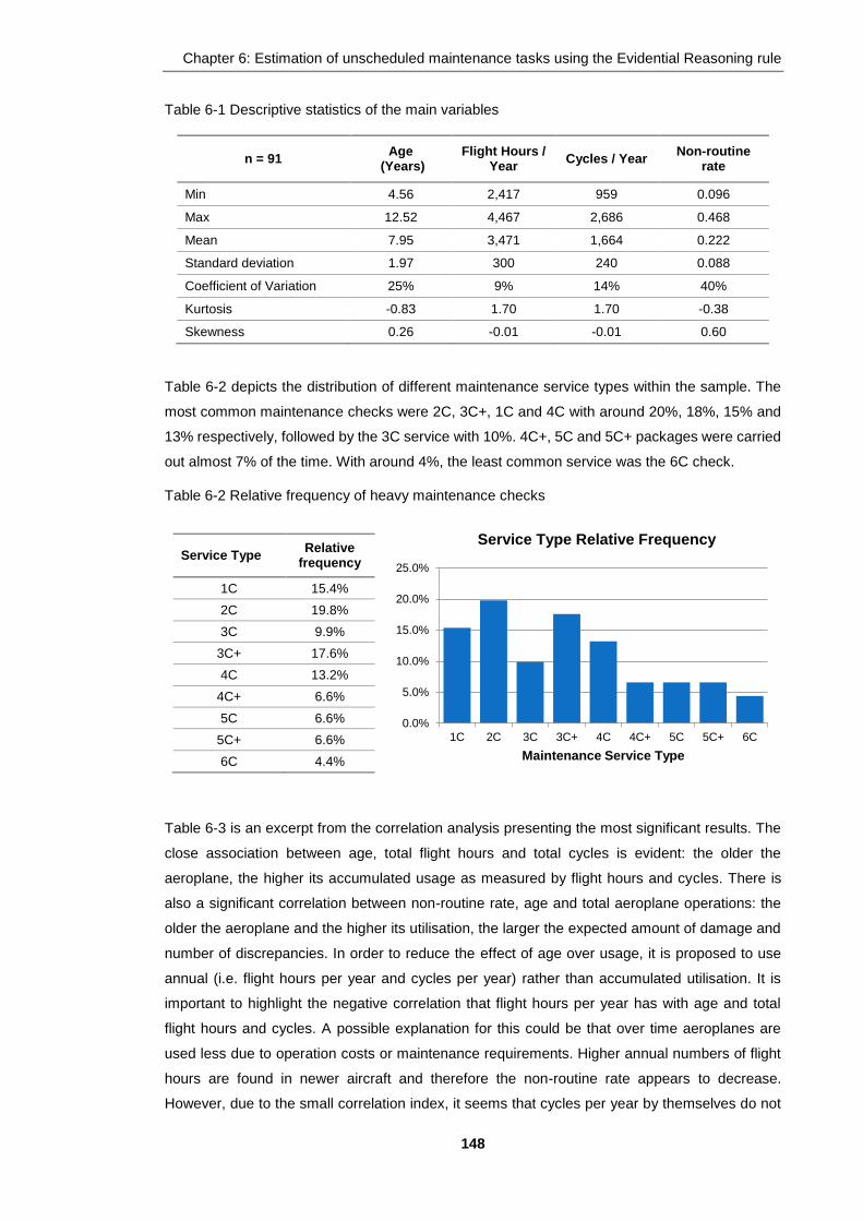
Chapter 6: Estimation of unscheduled maintenance tasks using the Evidential Reasoning rule
148
Table 6-1 Descriptive statistics of the main variables
n = 91 Age
(Years) Flight Hours /
Year Cycles / Year
Non-routine rate
Min 4.56 2,417 959 0.096
Max 12.52 4,467 2,686 0.468
Mean 7.95 3,471 1,664 0.222
Standard deviation 1.97 300 240 0.088
Coefficient of Variation 25% 9% 14% 40%
Kurtosis -0.83 1.70 1.70 -0.38
Skewness 0.26 -0.01 -0.01 0.60
Table 6-2 depicts the distribution of different maintenance service types within the sample. The
most common maintenance checks were 2C, 3C+, 1C and 4C with around 20%, 18%, 15% and
13% respectively, followed by the 3C service with 10%. 4C+, 5C and 5C+ packages were carried
out almost 7% of the time. With around 4%, the least common service was the 6C check.
Table 6-2 Relative frequency of heavy maintenance checks
Service Type Relative
frequency
1C 15.4%
2C 19.8%
3C 9.9%
3C+ 17.6%
4C 13.2%
4C+ 6.6%
5C 6.6%
5C+ 6.6%
6C 4.4%
Table 6-3 is an excerpt from the correlation analysis presenting the most significant results. The
close association between age, total flight hours and total cycles is evident: the older the
aeroplane, the higher its accumulated usage as measured by flight hours and cycles. There is
also a significant correlation between non-routine rate, age and total aeroplane operations: the
older the aeroplane and the higher its utilisation, the larger the expected amount of damage and
number of discrepancies. In order to reduce the effect of age over usage, it is proposed to use
annual (i.e. flight hours per year and cycles per year) rather than accumulated utilisation. It is
important to highlight the negative correlation that flight hours per year has with age and total
flight hours and cycles. A possible explanation for this could be that over time aeroplanes are
used less due to operation costs or maintenance requirements. Higher annual numbers of flight
hours are found in newer aircraft and therefore the non-routine rate appears to decrease.
However, due to the small correlation index, it seems that cycles per year by themselves do not
0.0%
5.0%
10.0%
15.0%
20.0%
25.0%
1C 2C 3C 3C+ 4C 4C+ 5C 5C+ 6C
Maintenance Service Type
Service Type Relative Frequency
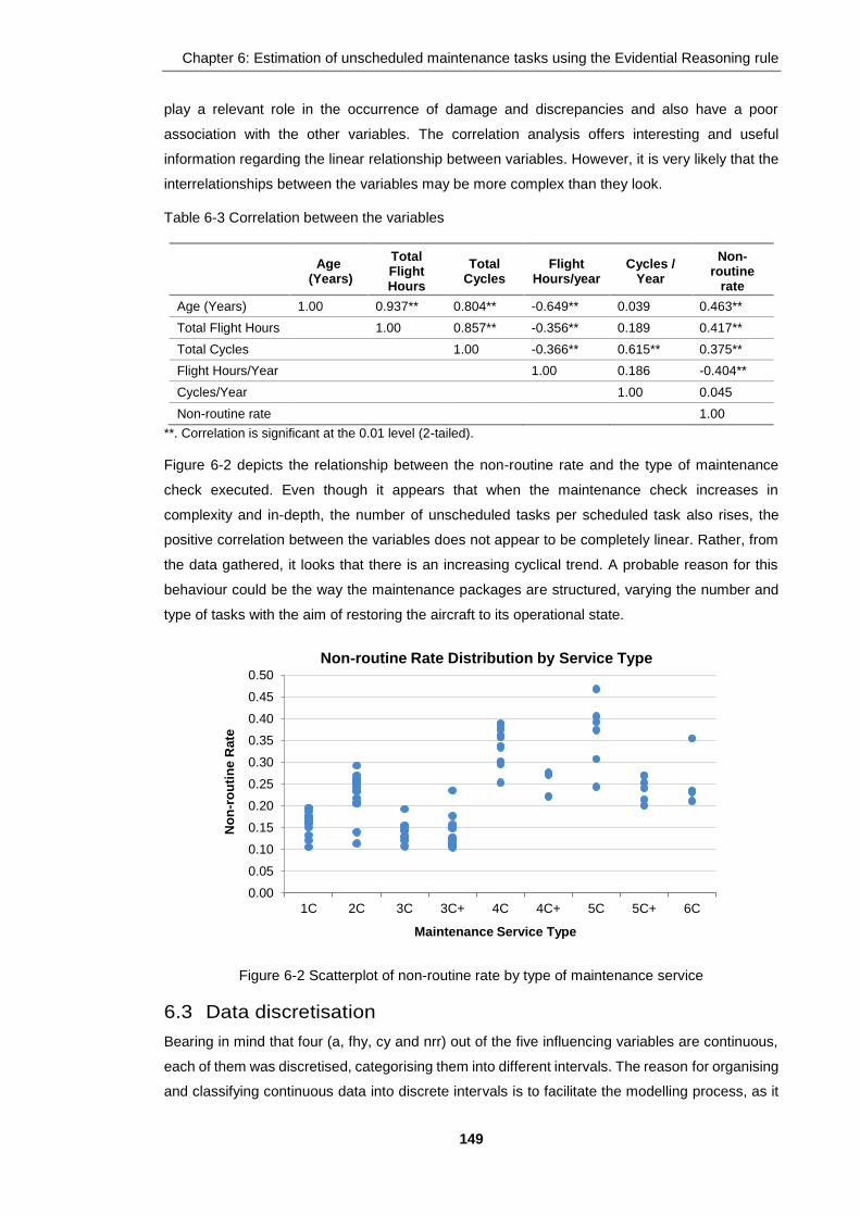
Chapter 6: Estimation of unscheduled maintenance tasks using the Evidential Reasoning rule
149
play a relevant role in the occurrence of damage and discrepancies and also have a poor
association with the other variables. The correlation analysis offers interesting and useful
information regarding the linear relationship between variables. However, it is very likely that the
interrelationships between the variables may be more complex than they look.
Table 6-3 Correlation between the variables
Age
(Years)
Total Flight Hours
Total Cycles
Flight Hours/year
Cycles / Year
Non-routine
rate
Age (Years) 1.00 0.937** 0.804** -0.649** 0.039 0.463**
Total Flight Hours 1.00 0.857** -0.356** 0.189 0.417**
Total Cycles 1.00 -0.366** 0.615** 0.375**
Flight Hours/Year 1.00 0.186 -0.404**
Cycles/Year 1.00 0.045
Non-routine rate 1.00
**. Correlation is significant at the 0.01 level (2-tailed).
Figure 6-2 depicts the relationship between the non-routine rate and the type of maintenance
check executed. Even though it appears that when the maintenance check increases in
complexity and in-depth, the number of unscheduled tasks per scheduled task also rises, the
positive correlation between the variables does not appear to be completely linear. Rather, from
the data gathered, it looks that there is an increasing cyclical trend. A probable reason for this
behaviour could be the way the maintenance packages are structured, varying the number and
type of tasks with the aim of restoring the aircraft to its operational state.
Figure 6-2 Scatterplot of non-routine rate by type of maintenance service
6.3 Data discretisation
Bearing in mind that four (a, fhy, cy and nrr) out of the five influencing variables are continuous,
each of them was discretised, categorising them into different intervals. The reason for organising
and classifying continuous data into discrete intervals is to facilitate the modelling process, as it
0.00
0.05
0.10
0.15
0.20
0.25
0.30
0.35
0.40
0.45
0.50
1C 2C 3C 3C+ 4C 4C+ 5C 5C+ 6C
No
n-r
ou
tin
e R
ate
Maintenance Service Type
Non-routine Rate Distribution by Service Type

Chapter 6: Estimation of unscheduled maintenance tasks using the Evidential Reasoning rule
150
helps to obtain the belief distributions (which will be described later). Moreover, by using discrete
or categorised information it is easier to understand and analyse for practitioners and decision
makers.
The discretisation process is carried out in three phases: 1) to properly categorise each variable,
the number of intervals and their width is obtained using different rules. 2) The interval widths
calculated in the previous step are reviewed and modified if necessary, to define intervals that
meaningfully represent the variables for experts and practitioners by using appropriate class limits
(e.g. it might be easier to conceptualise an age interval between 4 to 5 years than one of 4.37 to
5.66 years). 3) For each variable, different interval sizes are analysed comparing the shape of the
estimated density function to avoid under- or over-smoothing and to determine which describes
the data most precisely.
6.3.1 Determining the number of intervals and their width
Finding the correct number of intervals may not be an easy task. Doane (1976) raised the question
of how to calculate and make a frequency classification with the "right" number of classes, "nice"
class limits and "round" interval widths. In this regard, Guiasu (1986) explains that grouping data
is a useful way of dealing with complexity. However, he further adds that a certain amount of
information is lost when raw data is grouped in classes and that the larger the class interval, the
greater the amount of information that is lost. On the other hand, if the number of classes is too
large, the presentation of information can be misleading as it starts describing noises of the
sample. Therefore, Guiasu (1986) concludes that a reasonable balance between information
content and class homogeneity must be reached during the choice of a class interval.
Histograms are amongst the most important and useful graphical tools in statistical practice. They
are exceptionally helpful for displaying and summarising data and for providing a consistent
estimation and representation of any unknown density function (Scott, 2009). In the same vein,
Birgé and Rozenholc (2006) and Freedman and Diaconis (1981) remark that although histograms
may be considered an obsolete way of estimating densities, they are easy to produce and, unlike
kernel estimators, are widely used in applied work.
For building a regular histogram3, four basic parameters must be defined: 1) the lower and upper
limits of the sample; 2) the number of intervals, also called classes or bins; 3) the width of each
interval, or bin-width; and 4) the lower limit of the first interval.
The lower and upper limits of the sample (𝑎, 𝑏) are used to define the range of the dataset (𝑅 =
𝑏 − 𝑎) where the intervals are distributed. The number of classes (𝑘) determines the intervals in
which the raw data will be classified. The bin-width (ℎ) represents the length of each interval.
There is an inverse relation between the number of intervals and their width: the wider the bin,
the fewer intervals required and vice versa. In this regard, Wand (1997) explains that bin-width
3 A regular histogram is the one in which its intervals are of equal length (Birgé and Rozenholc, 2006). According to Scott (1992, 2009) to make the intervals comparable between them, they should have the same width, otherwise, if the interval widths are not of the same size, the shape of the histogram can be grossly misleading.

Chapter 6: Estimation of unscheduled maintenance tasks using the Evidential Reasoning rule
151
has a substantial effect on the appearance of the histogram with respect to the true distribution:
a very small bin-width produces a jagged histogram with too much detail (under-smoothing) and
conversely, a very large bin-width results in a histogram with not enough detail (over-
smoothing).The lower limit of the first class (𝑙0) also affects the shape of the histogram, as it
determines the position of the first bin and therefore the position of the others. Equation (6-1)
shows the relation between the upper and lower limits, the bin-width and the number of intervals.
As can be seen, the larger the range, the greater the number of intervals and the wider the bin
the smaller the number of intervals.
𝑘 =𝑏 − 𝑎
ℎ (6-1)
A plethora of rules has been proposed for determining the number of intervals and the bin width
for grouped data and the most common rules are described below.
6.3.1.1 Sturges’ rule:
Sturges’ rule (Sturges, 1926) is the most common rule for determining the number of intervals
and their width for histogram density estimation. It is a normal-based rule as it assumes that the
variable is normally distributed. The Gaussian variable is approximated to a binomial distribution
in order to divide it into equal sized intervals. In other words, a normally distributed sample of size
𝑛 can be divided in to 𝑘 intervals, so that the class frequencies comprise a binomial series for all
𝑛 which are powers of 2. Sturges’ rule converts continuous, symmetric, normal data into discrete,
symmetric, binomial classes (Doane, 1976). Equations (6-2) and (6-3) show Sturges’ rule, where
ℎ is the class width or class interval, 𝑘 represents the number of classes or bins, 𝑛 is the number
of elements of the sample and 𝑅 is the range.
𝑘 = 1 + 𝑙𝑜𝑔2𝑛 (6-2)
ℎ =𝑅
1 + 𝑙𝑜𝑔2𝑛 (6-3)
Despite its wide usage, several authors have criticised Sturges' rule, stating that, particularly for
large samples, severely skewed or multimodal distributions, it tends to over-smooth the
histogram, failing to provide enough classes to reveal the real shape of the distribution (Doane,
1976; Scott, 1992; Scott, 2009; Wand, 1997).
6.3.1.2 Doane’s rule:
Doane’s rule (Doane, 1976) is a modification of Sturges’ rule to overcome the problem of highly
skewed distributions. As can be seen in eq. (6-4), this rule includes an additional term to reflect
skewness. 𝑔1 (6-5) represents the moment coefficient of skewness and 𝜎𝑔1 (6-6) its standard
deviation, which becomes smaller as sample size increases. If the sample is symmetrical, 𝑔1 = 0,
no extra intervals are added and the rule becomes the same as Sturges’ rule.
𝑘 = 1 + 𝑙𝑜𝑔2𝑛 + 𝑙𝑜𝑔2 (1 +|𝑔1|
𝜎𝑔1
) (6-4)

Chapter 6: Estimation of unscheduled maintenance tasks using the Evidential Reasoning rule
152
𝑔1 =∑(𝑥 − �̅�)3
[∑(𝑥 − �̅�)2]3/2 (6-5)
𝜎𝑔1= √
6(𝑛 + 2)
(𝑛 + 1)(𝑛 + 3) (6-6)
6.3.1.3 Scott’s rule:
Scott’s rule (Scott, 1979), like Sturges' rule, also assumes a Gaussian distribution of the sample.
However, it is based on a different approach. This rule uses the integrated mean squared error
(IMSE) as a global error measure of a histogram to calculate the optimal bin width. The IMSE
compares the true density function, which is unknown, with the calculated histogram density.
Therefore, Scott assumed a normal distribution and used the Gaussian density function as a
reference. Eq. (6-7) presents Scott’s rule, where 𝑛 is the sample size and 𝜎 an estimate of the
standard deviation. Scott (2014) explains that both Sturges’ and Scott’s rules are based on the
normal distribution, but Sturges makes a deterministic calculation, whereas Scott’s approach is
based on optimising the global variance and squared bias of the histogram estimator.
Scott (1992) improved his rule (6-8) by adding two factors: the skewness and the kurtosis of the
sample. The skewness factor (6-9) considers a lognormal density function where 𝜎′ represents
the lognormal standard deviation. The kurtosis factor (6-10) uses a t distribution, where 𝑣 are the
degrees of freedom and Γ is the gamma distribution. These factors allow the rule to adjust the
interval width for samples that are not completely normal.
ℎ = 3.49𝜎𝑛−1/3 (6-7)
ℎ = 3.49𝜎𝑛−1/3(𝑆𝑘𝐹𝑐)(𝐾𝑢𝐹𝑐) (6-8)
𝑆𝑘𝐹𝑐 =21/3𝜎′
𝑒5𝜎′2/4(𝜎′2+2)1/3(𝑒𝜎′2−1)1/2
(6-9)
𝐾𝑢𝐹𝑐 =√𝑣 − 2
2[
Γ(𝑣 + 3)Γ (𝑣2
)2
Γ (𝑣 +32
) Γ (𝑣 + 3
2)
2]
1/3
(6-10)
6.3.1.4 Freedman-Diaconis’ rule:
Similarly to Scott’s rule, Freedman and Diaconis (1981) propose a formula to calculate the bin
width based on the IMSE, but instead of using the estimated standard deviation, they replace it
by utilising the interquartile range 𝐼𝑄 resulting in a more robust rule (6-11). According to Scott
(1992), the Freedman-Diaconis rule provides 35% more bins than Scott’s rule, giving a rougher
histogram. However, for highly skewed or spread samples this rule could be very useful.
ℎ = 2𝐼𝑄𝑛−1/3 (6-11)

Chapter 6: Estimation of unscheduled maintenance tasks using the Evidential Reasoning rule
153
6.3.1.5 Rules results and comparison
Table 6-4 shows a comparison of the number of intervals and the bin-width using the rules
described above. As can be seen, Sturges' rule suggests the same number of intervals (near 8)
for the different variables, as the rule relies just on the size of the sample. Therefore, as the
sample size is the same for all variables, the number of intervals remains the same. Doane's rule
modifies Sturge's rule by adding the skewness effect. It can be seen that as age and non-routine
rate are more skewed than flight hours and cycles, they require more intervals (around 9-10) than
the latter (approx. 8). Scott's rule takes into account the dispersion of the data by using the
standard deviation. According to the suggested number of intervals, the flight hours and cycles
are more dispersed than age and non-routine rate. However, after considering the effect of
skewness and kurtosis, it seems that these factors have greater impact on the number of intervals
for age and non-routine rate (i.e. the enhanced Scott's rule suggests around 6-7 intervals for a
and nrr, and 9-10 for fhy and cy). Similarly to Scott's rule, the Freedman-Diaconis rule also
considers the data spread, but based on the interquartile range of the sample. His rule suggests
more intervals for flight hours and cycles. In summary, these rules propose using a bin-width from
0.9 to 1.5 years for aircraft age, a bin-width of around 144 to 273 hours for flight hours, an interval-
width between 74 and 230 cycles for take-off-landings and a class-width from 0.05 to 0.07 for
non-routine rate.
Table 6-4 Number of intervals “k” and bin-widths “h” according to different rules.
Rules Age Flight
hours/year Cycles/year
Non-routine rate
h k h k h k h k
Sturge's 1.1 7.5 273 7.5 230 7.5 0.05 7.5
Doane's 0.9 8.5 270 7.6 228 7.6 0.04 9.3
Scott's (Normal) 1.5 5.2 233 8.8 186 9.3 0.07 5.5
Scott's (w/Sk& Ku factors) 1.4 5.8 228 9.0 178 9.7 0.05 7.0
Freedman-Diaconis' 1.5 5.4 144 14.2 74 23.4 0.05 6.9
6.3.2 Intervals meaningfulness
The results obtained in Table 6-4 were reviewed and adjusted to take into account their
meaningfulness and practicality for practitioners and experts. The class intervals are redefined to
improve understanding and utilisation. Table 6-5 presents the suggested bin-widths for each
variable. For aircraft age, it may be clearer to work with periods of one year or half a year and a
bin width of 0.5, 1, 1.5 or 2 years of age is therefore recommended. For the interval-widths of
flight hours and cycles, it is proposed to utilise multiples of 50 (i.e. 150, 200, 250 and 300). Non-
routine rate is easier to handle with bin-widths of 0.025, 0.05 or 0.10.

Chapter 6: Estimation of unscheduled maintenance tasks using the Evidential Reasoning rule
154
Table 6-5 Proposed number of intervals and bin-widths
Option Age Flight hours/year Cycles/year Non-routine rate
h k h k h k h k
1 0.5 15.9 150 13.7 150 11.5 0.025 14.9
2 1.0 8.0 200 10.3 200 8.6 0.05 7.4
3 1.5 5.3 250 8.2 250 6.9 0.10 3.7
4 2.0 4.0 300 6.8 300 5.8
6.3.3 Data distribution
Using the bin-widths proposed in Table 6-5, several frequency distribution graphs were created
for each variable with the aim of comparing their shapes and determining those that are most
suitable for representing the data. The graphs were built using different interval sizes and by
moving the lower limit of the first interval.
Figure 6-3 illustrates the frequency distribution of the sample for aircraft age when the bin size is
half a year (i.e. 0.5). Figure 6-4 depicts the frequency distribution with a bin-width of two years
(i.e. 2.0). These figures show the effect of the interval-width on the shape of the distribution. It
can clearly be seen that in the first graph the distribution appears to be jagged, while the second
has an over-smoothed shape. Using the same bin-width but with different interval limits can also
affect the shape of the distribution. Figure 6-5 and Figure 6-6 present an example of this situation.
Both histograms have a bin-width of 1.5 years, but the lower limit of the first graph is 2.5 years,
whereas for the second it is 3.0 years. It is noticeable that the shape of the distribution is
significantly different between the two histograms. Therefore, it is important to highlight the
relevance of choosing the most appropriate bin-width and interval limits, as they might change
the shape the frequency distribution and subsequently affect calculation of the belief distribution,
so altering the results and performance of the ER model. In a similar way to this example, Table
B-2, Table B-3, Table B-4 and Table B-5 in Appendix B.2 show the comparison of different
frequency distributions for the four variables (age, flight hours, cycles and non-routine rate,
respectively).
Figure 6-3 Aircraft's age frequency
distribution with a bin-width of 0.5 years
Figure 6-4 Aircraft's age frequency
distribution with a bin-width of 2.0 years
0.00
0.05
0.10
0.15
0.20
0.25
Rela
tive F
req
uen
cy
Aircraft's Age
Aircraft's Age Frequency Distribution
0.00
0.05
0.10
0.15
0.20
0.25
0.30
0.35
Re
lati
ve F
req
uen
cy
Aircraft's Age
Aircraft's Age Frequency Distribution

Chapter 6: Estimation of unscheduled maintenance tasks using the Evidential Reasoning rule
155
Figure 6-5 Aircraft's age frequency
distribution with a bin-width of 1.5 year, lower
limit 2.5
Figure 6-6 Aircraft's age frequency
distribution with a bin-width of 1.5 year, lower
limit 3.0
6.4 ER rule model
After performing this brief statistical analysis, and once the variables have been discretised into
different intervals, the evidential reasoning (ER) rule, a generic Bayesian reasoning process for
combining multiple pieces of independent evidence, is applied to develop an inference model for
estimating unscheduled activities in aircraft maintenance. The procedure described below is
based on Yang and Xu (2014) and is used for building the inference model.
1. Determine the frequency distribution between the intervals of the predictor variables and
the classes of the observed outcome (i.e. non-routine rate) using a cross-tabulation. For
example, given a specific age bin, determine the number of maintenance services that fit
into a particular range of non-routine rate.
2. Based on the frequency distribution, the prior probabilities of the non-routine rate and the
likelihoods for each interval of every variable are calculated.
a. The prior probabilities are obtained by dividing the frequency of each non-routine
interval by the total number of maintenance services. In other words, the prior
probabilities represent the relative frequency of the non-routine rate.
b. The likelihoods are determined for each non-routine rate interval, dividing the
number of events for every interval of the predictor variables by the frequency of
that particular non-routine rate interval.
3. Using the results of step 2, the belief distributions for each interval of the predictor
variables (pieces of evidence) are obtained by dividing each likelihood by the sum of
likelihoods in that class.
4. The ER rule is applied to aggregate two classes of different pieces of evidence, combining
the non-routine rate belief distribution of the first variable with the non-routine rate belief
distribution of the second variable. Then, the ER rule is used recursively to aggregate all
the other pieces of evidence to finally obtain the belief distribution of the expected non-
routine rate.
0.00
0.05
0.10
0.15
0.20
0.25
0.30
0.35
Rela
tive F
req
uen
cy
Aircraft's Age
Aircraft's Age Frequency Distribution
0.00
0.05
0.10
0.15
0.20
0.25
0.30
Rela
tive F
req
uen
cy
Aircraft's Age
Aircraft's Age Frequency Distribution

Chapter 6: Estimation of unscheduled maintenance tasks using the Evidential Reasoning rule
156
In order to clarify the described process, the subsequent paragraphs present an easy-to-follow
example based on the collected maintenance records. An essential step before beginning this
process is the definition of intervals for each variable. For the presented example, they are set as
follows: 1) five classes for non-routine rate with a bin-width of 0.1, starting from 0 and ending in
0.5; 2) for age, five intervals of two years each with a lower limit of 4 years and an upper limit of
14; 3) nine bins of 250 flight hours each, ranging from 2250 to 4500; 4) eight classes with a size
of 250 cycles, between 750 and 2750; and 5) services type, as a categorical variable, considers
the nine different types of maintenance checks applied.
Firstly, each maintenance event in the sample is counted and allocated to its corresponding
interval, building a matrix of frequencies between each variable and the non-routine rate. For
instance, of the 35 aeroplanes aged between 6 and 8 years, 12 have a non-routine rate from
0.10-0.20, 14 a rate of 0.20-0.30 and nine a rate from 0.30-0.40 (shown in row 2 Table 6-6). The
frequency distribution of the non-routine rate was obtained in the same way for the rest of the
variables. The results can be seen in Table 6-6.
Table 6-6 Non-routine rate frequency distribution of each piece of evidence
Row Variable Interval
Non-routine Rate (NRT/RT)
Total 0-0.1 0.1-0.2
0.2-0.3
0.3-0.4
0.4-0.5
1
Age
4-6 1 20 1 22
2 6-8 12 14 9 35
3 8-10 16 4 2 22
4 10-12 7 3 1 11
5 12-14 1 1
6 Total Age 1 39 35 14 2 91
7
Flight hours / Year
2250-2500 1 1
8 2500-2750 0
9 2750-3000 2 3 1 6
10 3000-3250 2 1 1 4
11 3250-3500 10 16 11 2 39
12 3500-3750 1 12 11 1 25
13 3750-4000 11 3 14
14 4000-4250 1 1
15 4250-4500 1 1
16 Total Fh / Y 1 39 35 14 2 91
17
Cycles / Year
750-1000 1 1
18 1000-1250 3 3
19 1250-1500 9 5 1 15
20 1500-1750 19 18 8 2 47
21 1750-2000 1 10 5 5 21
22 2000-2250 2 2
23 2250-2500 0
24 2500-2750 1 1 2
25 Total Cy / Y 1 39 35 14 2 91

Chapter 6: Estimation of unscheduled maintenance tasks using the Evidential Reasoning rule
157
Row Variable Interval
Non-routine Rate (NRT/RT)
Total 0-0.1 0.1-0.2
0.2-0.3
0.3-0.4
0.4-0.5
26
Maintenance Service Type
1C 14 14
27 2C 2 16 18
28 3C 9 9
29 3C+ 1 14 1 16
30 4C 2 10 12
31 4C+ 6 6
32 5C 1 3 2 6
33 5C+ 6 6
34 6C 3 1 4
35 Total Services 1 39 35 14 2 91
The prior probabilities and likelihoods for each variable are then generated. Continuing with this
example, the prior probability is calculated by dividing the frequency of the non-routine rate by the
total number of events, i.e. 1/91, 39/91, 35/91, 14/91 and 2/91 correspondingly (rows 6, 16, 25 or
35 in Table 6-6 and the results in rows 6, 16, 25 or 35 in Table 6-7). The likelihoods are obtained
by dividing the non-routine rate frequency of a particular piece of evidence by the total frequency
of that specific non-routine rate interval. In the case of an aeroplane between 6 and 8 years old,
this means dividing its specific non-routine frequency by the total non-routine frequency of each
interval, namely 12/39, 14/35 and 9/14 (row 2 over row 6 of Table 6-6; results in row 2 Table 6-7).
Table 6-7 presents the prior probabilities and likelihoods of all pieces of evidence, with the
examples highlighted. The likelihood of aircraft aged between 6 and 8 years represent 31% of
maintenance services with a non-routine rate of 0.10-0.20, 40% with a non-routine rate from 0.20-
0.30 and 64% with a non-routine rate of 0.30-0.40. None of this class of aircraft have a non-routine
rate between 0 and 0.10, or 0.40 and 0.50 (highlighted in row 2 Table 6-7).
Table 6-7 Prior probabilities and likelihoods of each piece of evidence
row Variable Interval Non-routine Rate (NRT/RT)
0-0.1 0.1-0.2 0.2-0.3 0.3-0.4 0.4-0.5
1 Age 4-6 1.000 0.513 0.029 - -
2 6-8 - 0.308 0.400 0.643 -
3 8-10 - - 0.457 0.286 1.000
4 10-12 - 0.179 0.086 0.071 -
5 12-14 - - 0.029 - -
6 Prior probability 0.011 0.429 0.385 0.154 0.022
7
Flight hours /Year
2250-2500 - - 0.029 - -
8 2500-2750 - - - - -
9 2750-3000 - 0.051 0.086 0.071 -
10 3000-3250 - 0.051 0.029 0.071 -
11 3250-3500 - 0.256 0.457 0.786 1.000
12 3500-3750 1.000 0.308 0.314 0.071 -
13 3750-4000 - 0.282 0.086 - -
14 4000-4250 - 0.026 - - -

Chapter 6: Estimation of unscheduled maintenance tasks using the Evidential Reasoning rule
158
row Variable Interval Non-routine Rate (NRT/RT)
0-0.1 0.1-0.2 0.2-0.3 0.3-0.4 0.4-0.5
15 4250-4500 - 0.026 - - -
16 Prior probability 0.011 0.429 0.385 0.154 0.022
17
Cycles /Year
750-1000 - - 0.029 - -
18 1000-1250 - - 0.086 - -
19 1250-1500 - 0.231 0.143 0.071 -
20 1500-1750 - 0.487 0.514 0.571 1.000
21 1750-2000 1.000 0.256 0.143 0.357 -
22 2000-2250 - - 0.057 - -
23 2250-2500 - - - - -
24 2500-2750 - 0.026 0.029 - -
25 Prior probability 0.011 0.429 0.385 0.154 0.022
26
Maintenance Service Type
1C - 0.359 - - -
27 2C - 0.051 0.457 - -
28 3C - 0.231 - - -
29 3C+ 1.000 0.359 0.029 - -
30 4C - - 0.057 0.714 -
31 4C+ - - 0.171 - -
32 5C - - 0.029 0.214 1.000
33 5C+ - - 0.171 - -
34 6C - - 0.086 0.071 -
35 Prior probability 0.011 0.429 0.385 0.154 0.022
The third step is to calculate the belief distributions for each piece of evidence, where each
likelihood of a particular category is divided by the sum of likelihoods of that class. Following the
example of aircraft aged between 6 and 8 years, the non-routine rate belief distribution of 0.228,
0.296 and 0.476 (shown in row 2 Table 6-8) is calculated by dividing 0.31 by the sum of 0.31,
0.40 and 0.64 (i.e. 1.35), 0.40 by 1.35 and 0.64 by 1.35 respectively (i.e. dividing each likelihood
in row 2 Table 6-7 by the sum of those likelihoods). For this particular case, the belief distribution
can be explained as the possibility of having a non-routine rate of 0.10 to 0.20 22.3% of the time,
in 29.6% of the occasions a non-routine rate from 0.20 to 0.30 and a 47.6% chance of a non-
routine rate between 0.30 and 0.40. Table 6-8 shows the non-routine rate belief distributions for
each piece of evidence.
Table 6-8 Non-routine rate belief distribution of each piece of evidence
row Variable Interval Non-routine Rate (NRT/RT)
0-0.1 0.1-0.2 0.2-0.3 0.3-0.4 0.4-0.5
1
Age
4-6 0.649 0.333 0.019 - -
2 6-8 - 0.228 0.296 0.476 -
3 8-10 - - 0.262 0.164 0.574
4 10-12 - 0.533 0.255 0.212 -
5 12-14 - - 1.000 - -
6 Flight hours / Year
2250-2500 - - 1.000 - -
7 2500-2750 - - - - -
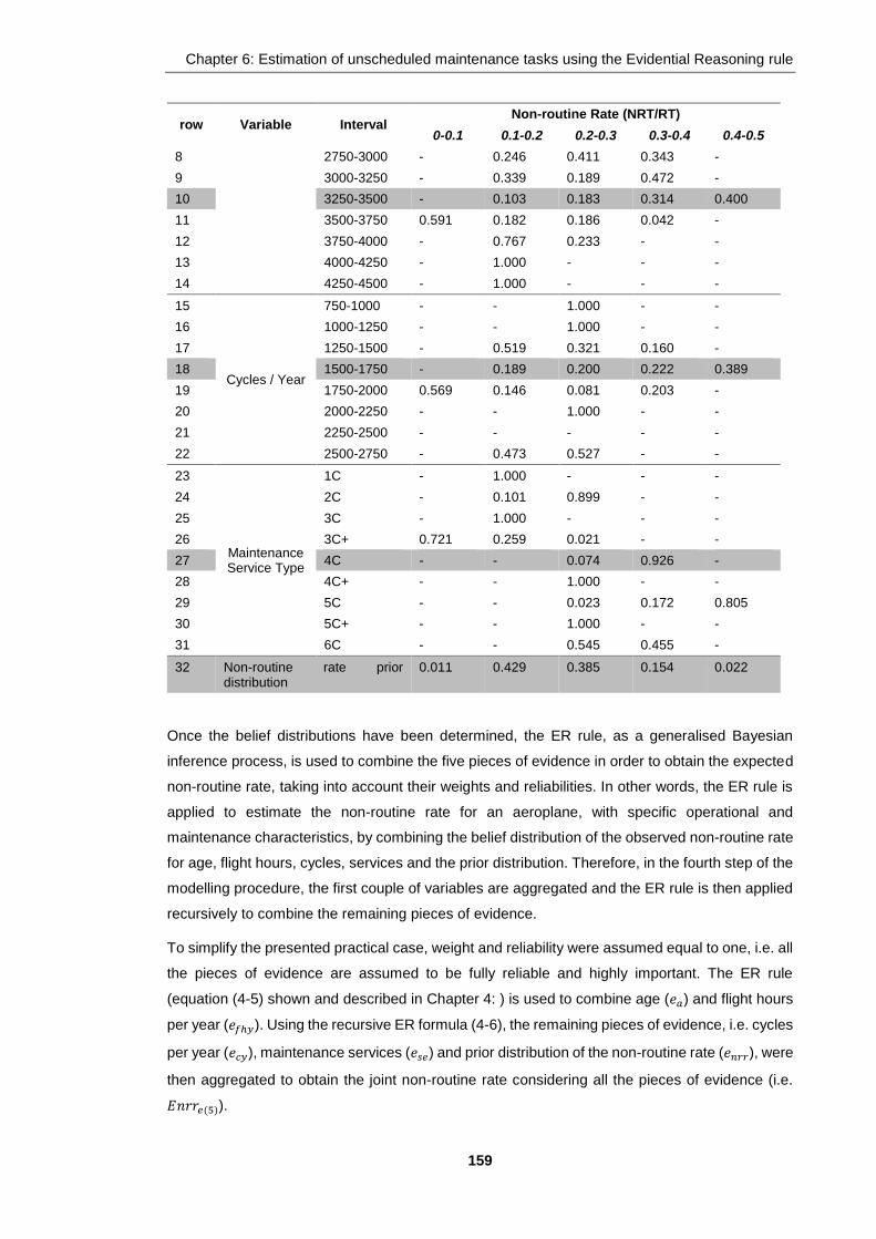
Chapter 6: Estimation of unscheduled maintenance tasks using the Evidential Reasoning rule
159
row Variable Interval Non-routine Rate (NRT/RT)
0-0.1 0.1-0.2 0.2-0.3 0.3-0.4 0.4-0.5
8 2750-3000 - 0.246 0.411 0.343 -
9 3000-3250 - 0.339 0.189 0.472 -
10 3250-3500 - 0.103 0.183 0.314 0.400
11 3500-3750 0.591 0.182 0.186 0.042 -
12 3750-4000 - 0.767 0.233 - -
13 4000-4250 - 1.000 - - -
14 4250-4500 - 1.000 - - -
15
Cycles / Year
750-1000 - - 1.000 - -
16 1000-1250 - - 1.000 - -
17 1250-1500 - 0.519 0.321 0.160 -
18 1500-1750 - 0.189 0.200 0.222 0.389
19 1750-2000 0.569 0.146 0.081 0.203 -
20 2000-2250 - - 1.000 - -
21 2250-2500 - - - - -
22 2500-2750 - 0.473 0.527 - -
23
Maintenance Service Type
1C - 1.000 - - -
24 2C - 0.101 0.899 - -
25 3C - 1.000 - - -
26 3C+ 0.721 0.259 0.021 - -
27 4C - - 0.074 0.926 -
28 4C+ - - 1.000 - -
29 5C - - 0.023 0.172 0.805
30 5C+ - - 1.000 - -
31 6C - - 0.545 0.455 -
32 Non-routine rate prior distribution
0.011 0.429 0.385 0.154 0.022
Once the belief distributions have been determined, the ER rule, as a generalised Bayesian
inference process, is used to combine the five pieces of evidence in order to obtain the expected
non-routine rate, taking into account their weights and reliabilities. In other words, the ER rule is
applied to estimate the non-routine rate for an aeroplane, with specific operational and
maintenance characteristics, by combining the belief distribution of the observed non-routine rate
for age, flight hours, cycles, services and the prior distribution. Therefore, in the fourth step of the
modelling procedure, the first couple of variables are aggregated and the ER rule is then applied
recursively to combine the remaining pieces of evidence.
To simplify the presented practical case, weight and reliability were assumed equal to one, i.e. all
the pieces of evidence are assumed to be fully reliable and highly important. The ER rule
(equation (4-5) shown and described in Chapter 4: ) is used to combine age (𝑒𝑎) and flight hours
per year (𝑒𝑓ℎ𝑦). Using the recursive ER formula (4-6), the remaining pieces of evidence, i.e. cycles
per year (𝑒𝑐𝑦), maintenance services (𝑒𝑠𝑒) and prior distribution of the non-routine rate (𝑒𝑛𝑟𝑟), were
then aggregated to obtain the joint non-routine rate considering all the pieces of evidence (i.e.
𝐸𝑛𝑟𝑟𝑒(5)).

Chapter 6: Estimation of unscheduled maintenance tasks using the Evidential Reasoning rule
160
The example continues by considering the non-routine rate distribution of the whole sample and
an aeroplane aged between 6 and 8 years old, with a yearly utilisation of 3,250-3,500 flight hours
and 1,500-1,750 cycles and which underwent a 4C maintenance check (rows 2, 10, 18, 27 and
32 in Table 6-8). The combined degree of belief of the five pieces of evidence is given in Table
6-9. Rows 2-6 present the belief distribution of the non-routine rate for each piece of evidence. In
rows 7-11, the weighted belief distribution is calculated using 𝑚𝜃,𝑗 = 𝑤𝑗𝑝𝜃,𝑗, in this case as 𝑤𝑗 =
1, 𝑚𝜃,𝑗 = 𝑝𝜃,𝑗. In rows 12 and 13, the ER rule, eq. (4-5) is used to combine the first two pieces of
evidence, i.e. age (𝑒𝑎) and flight hours per year (𝑒𝑓ℎ𝑦). Then, in rows 14 to 19 the ER rule is
applied recursively, eq. (4-6), to aggregate the remaining variables. In the last row, the combined
belief distribution of the non-routine rate, based on the information provided by the five pieces of
evidence, is shown. As can be seen in row 20, for an aeroplane with the aforementioned
characteristics, the expected belief distribution of the non-routine rate is a 6% chance for a rate
between 0.20 and 0.30 and a 94% possibility for a rate from 0.3 to 0.4. Figure 6-7 depicts the
aggregation process using the ER Rule for the example described above. Here, it is interesting
to observe how the belief distribution changes shape with each iteration.
Table 6-9 ER Rule for an aeroplane aged 6-8, with 3,250-3,500 fh/y, 1500-1750 cy/y and a 4C
service.
Non-routine rate
0-0.1 0.1-0.2 0.2-0.3 0.3-0.4 0.4-0.5 P(Θ)
2 pθ,a - 0.228 0.296 0.476 - -
3 pθ,fhy - 0.103 0.183 0.314 0.400 -
4 pθ,cy - 0.189 0.200 0.222 0.389 -
5 pθ,se - - 0.074 0.926 - -
6 pθ,nrr 0.011 0.429 0.385 0.154 0.022 -
7 mθ,a - 0.228 0.296 0.476 - -
8 mθ,fhy - 0.103 0.183 0.314 0.400 -
9 mθ,cy - 0.189 0.200 0.222 0.389 -
10 mθ,se - - 0.074 0.926 - -
11 mθ,nrr 0.011 0.429 0.385 0.154 0.022 -
12 m̂θ,e(2) - 0.023 0.054 0.150 - -
13 mθ,e(2) - 0.103 0.238 0.659 - -
14 m̂θ,e(3) - 0.019 0.048 0.146 - -
15 mθ,e(3) - 0.091 0.223 0.685 - -
16 m̂θ,e(4) - - 0.017 0.635 - -
17 mθ,e(4) - - 0.025 0.975 - -
18 m̂θ,e(5) - - 0.010 0.150 - -
19 mθ,e(5) - - 0.061 0.939 - -
20 Enrrθ,e(5) - - 0.061 0.939 -

Chapter 6: Estimation of unscheduled maintenance tasks using the Evidential Reasoning rule
161
Figure 6-7 ER Rule for an aeroplane aged 6-8, with 3,250-3,500 fh/y, 1500-1750 cy/y and a 4C service.
0.00.10.20.30.40.50.60.70.80.91.0
0-0.1 0.1-0.2 0.2-0.3 0.3-0.4 0.4-0.5
Non-routine rate (nrr)
Non-routine rate distribution for Age 6-8 years
0.00.10.20.30.40.50.60.70.80.91.0
0-0.1 0.1-0.2 0.2-0.3 0.3-0.4 0.4-0.5
Non-routine rate (nrr)
Non-routine rate distribution for Age and Flight hrs/year
0.00.10.20.30.40.50.60.70.80.91.0
0-0.1 0.1-0.2 0.2-0.3 0.3-0.4 0.4-0.5
Non-routine rate (nrr)
Non-routine rate distribution for Flight hrs/year 3,250-3,500
0.00.10.20.30.40.50.60.70.80.91.0
0-0.1 0.1-0.2 0.2-0.3 0.3-0.4 0.4-0.5
Non-routine rate (nrr)
Non-routine rate distribution for Cycles/year 1,500-1,750
0.00.10.20.30.40.50.60.70.80.91.0
0-0.1 0.1-0.2 0.2-0.3 0.3-0.4 0.4-0.5
Non-routine rate (nrr)
Non-routine rate distribution for Age, Fhy, Cy and Se
0.00.10.20.30.40.50.60.70.80.91.0
0-0.1 0.1-0.2 0.2-0.3 0.3-0.4 0.4-0.5
Non-routine rate (nrr)
Non-routine rate distribution for Age, Fhy and Cy
0.00.10.20.30.40.50.60.70.80.91.0
0-0.1 0.1-0.2 0.2-0.3 0.3-0.4 0.4-0.5
Non-routine rate (nrr)
Non-routine rate distribution for Maintenace service 4C
0.00.10.20.30.40.50.60.70.80.91.0
0-0.1 0.1-0.2 0.2-0.3 0.3-0.4 0.4-0.5
Non-routine rate (nrr)
Non-routine rate distribution for Prior distribution
0.00.10.20.30.40.50.60.70.80.91.0
0-0.1 0.1-0.2 0.2-0.3 0.3-0.4 0.4-0.5
Non-routine rate (nrr)
Expected Non-routine rate distribution
ER rule
ER rule
ER rule
ER rule

Chapter 6: Estimation of unscheduled maintenance tasks using the Evidential Reasoning rule
162
Table 6-9 and Figure 6-7 describe the ER Rule aggregation process for a specific array of
variables. There are 3,240 potential variable combinations, considering the intervals defined
above (i.e. five classes for age, nine for flight hours per year, eight for cycles per year and nine
for the type of maintenance service). The same process, therefore, should be applied 3,239 more
times to obtain the expected belief distribution for all the possible cases. On the other hand,
analysing the real data, just 43 real combinations are found, so in order to reduce computation
time, the aggregation process is applied only for the actual cases. Table 6-10 presents the
expected non-routine rate for the 43 real cases.
As can be noted from the description of the ER model, the aggregation process to estimate the
non-routine rate for the different combinations of Age-Flight hours-Cycles-Services requires
recurrent and extensive calculations even for the small sample used in the study. Performing all
these mathematical operations manually would be tedious, inefficient and time consuming.
Working with a traditional spreadsheet application would not be the best option as such software
is not capable of working with a large amount of variables, especially for the optimisation models.
For this reason, to reduce calculation time and to make the model more robust in handling a large
number of variables and more responsive to changes, MATLAB is used to build the different
aggregation models to address the scenarios that will be described in the following sections.
Table 6-10 Expected non-routine rate belief distribution for the real combinations
Age Hours Cycles Services Enrrθ,e(5) Estimated non-routine rate
0-0.1 0.1-0.2 0.2-0.3 0.3-0.4 0.4-0.5
4-6 3500-3750 1500-1750 3C - 1.000 - - -
4-6 3500-3750 1500-1750 3C+ - 0.996 0.004 - -
4-6 3500-3750 1750-2000 3C+ 0.638 0.361 0.001 - -
4-6 3750-4000 1250-1500 1C - 1.000 - - -
4-6 3750-4000 1250-1500 2C - 0.923 0.077 - -
4-6 3750-4000 1250-1500 3C - 1.000 - - -
4-6 3750-4000 1250-1500 3C+ - 0.999 0.001 - -
4-6 3750-4000 1500-1750 1C - 1.000 - - -
4-6 3750-4000 1500-1750 3C - 1.000 - - -
4-6 4000-4250 1500-1750 3C+ - 1.000 - - -
4-6 4250-4500 1750-2000 3C - 1.000 - - -
6-8 3250-3500 1500-1750 1C - 1.000 - - -
6-8 3250-3500 1500-1750 4C - - 0.061 0.939 -
6-8 3250-3500 1750-2000 1C - 1.000 - - -
6-8 3250-3500 1750-2000 4C - - 0.028 0.972 -
6-8 3250-3500 1750-2000 4C+ - - 1.000 - -
6-8 3500-3750 1500-1750 1C - 1.000 - - -
6-8 3500-3750 1500-1750 2C - 0.082 0.918 - -
6-8 3500-3750 1500-1750 3C+ - 0.909 0.091 - -
6-8 3500-3750 1500-1750 4C - - 0.330 0.670 -

Chapter 6: Estimation of unscheduled maintenance tasks using the Evidential Reasoning rule
163
6-8 3500-3750 1500-1750 4C+ - - 1.000 - -
6-8 3500-3750 1750-2000 4C+ - - 1.000 - -
6-8 3750-4000 1500-1750 2C - 0.231 0.769 - -
8-10 2250-2500 750-1000 2C - - 1.000 - -
8-10 3000-3250 1500-1750 2C - - 1.000 - -
8-10 3000-3250 1750-2000 5C - - 0.079 0.921 -
8-10 3250-3500 1000-1250 5C+ - - 1.000 - -
8-10 3250-3500 1500-1750 2C - - 1.000 - -
8-10 3250-3500 1500-1750 4C - - 0.144 0.856 -
8-10 3250-3500 1500-1750 5C - - 0.043 0.154 0.802
8-10 3250-3500 2000-2250 5C+ - - 1.000 - -
8-10 3500-3750 1000-1250 5C+ - - 1.000 - -
8-10 3500-3750 1250-1500 5C+ - - 1.000 - -
10-12 2750-3000 1250-1500 1C - 1.000 - - -
10-12 2750-3000 1250-1500 3C+ - 0.966 0.034 - -
10-12 2750-3000 1250-1500 6C - - 0.896 0.104 -
10-12 3000-3250 1500-1750 1C - 1.000 - - -
10-12 3000-3250 1500-1750 3C+ - 0.980 0.020 - -
10-12 3250-3500 1750-2000 3C+ - 0.967 0.033 - -
10-12 3500-3750 1750-2000 3C+ - 0.981 0.019 - -
10-12 3750-4000 2500-2750 3C - 1.000 - - -
10-12 3750-4000 2500-2750 6C - - 1.000 - -
12-14 2750-3000 1000-1250 2C - - 1.000 - -
To evaluate the performance of the model, four main indicators are used: 1) Mean Square Error
(MSE); 2) Mean Absolute Error (MAE); 3) Mean Absolute Percentage Error (MAPE) and 4) Mean
Accuracy Indicator (MAI).
Considering 𝑥𝑒𝑠𝑡 as the estimated or predicted value by the model, 𝑥𝑎𝑐𝑡 as the observed or real
value and 𝑛 as the number of elements, the MSE is the sum of the squared differences between
the predicted and observed values, divided by the number of elements, as shown in eq. (6-12).
The MAE is the sum of the absolute differences between the predicted and observed values,
divided by the number of elements, as shown in eq. (6-13). The MAPE is expressed as the
absolute value resulting from the difference between the predicted and the observed outcomes
divided by the observed outcome. All the absolute values are summed and then divided by the
number of elements and finally multiplied by 100 to express it as a percentage, as shown in eq.
(6-14). The MAI is a proposed indicator to measure the efficiency of the model and is represented
as the average of the accuracies of all maintenance services. The accuracy of each maintenance
service is calculated by the complement of the relation between the absolute difference of the
predicted and observed values and the maximum error amongst these two measures (i.e. the
maximum possible difference), as shown in eq. (6-15).

Chapter 6: Estimation of unscheduled maintenance tasks using the Evidential Reasoning rule
164
𝑀𝑆𝐸 =∑(𝑥𝑒𝑠𝑡 − 𝑥𝑎𝑐𝑡)2
𝑛 (6-12)
𝑀𝐴𝐸 =∑|𝑥𝑒𝑠𝑡 − 𝑥𝑎𝑐𝑡|
𝑛 (6-13)
𝑀𝐴𝑃𝐸 =∑ |
𝑥𝑒𝑠𝑡 − 𝑥𝑎𝑐𝑡
𝑥𝑎𝑐𝑡|
𝑛∗ 100
(6-14)
𝑀𝐴𝐼 =
∑ (1 −|𝑥𝑒𝑠𝑡 − 𝑥𝑎𝑐𝑡|
𝑒𝑟𝑟𝑀𝐴𝑋)
𝑛∗ 100
(6-15)
For the proposed model, the MSE is used to assess the performance in two stages. Firstly, it
compares the estimated non-routine belief distribution with the actual distribution, based on real
data. Secondly, it evaluates the difference between the estimated non-routine rate and the
observed rate for each maintenance service in the sample, i.e. a one-to-one comparison. To
differentiate these indicators, the former will be referred to as MSEDIST and the latter as MSESERV.
The other indicators (MAE, MAPE and MAI) are exclusively used to compare the estimated non-
routine rate for each maintenance service against its recorded counterpart.
Table B-6 and Table B-7 are based on the estimated non routine rate presented in Table 6-10
and the actual rate observed in the sample (Table B-1 in Appendix B.1) and are displayed in
Appendix B.3. Table B-6 compares the estimated non-routine rate distribution with its real
counterpart. Here the MSEDIST is used to assess the differences between the two distributions.
Table B-7 shows the estimated average and the observed non-routine rates. In this case
MSESERV, MAE, MAPE and MAI are used to compare these rates and to assess the model
performance.
Comparing the estimated against the recorded values, the results of the indicators are as follows:
MSEDIST = 0.0202, MSESERV = 0.0017, MAE = 0.0302, MAPE = 16.3%, MAI = 93.3%. The average
square error of the belief distribution is 0.0202, while the average square error of the non-routine
rate is 0.0017. The MAPE indicates that the error of the model is 16.3% in average, whereas the
MAE suggests that the model deviates ±0.0302 non-routine rate in average. The MAI expresses
that the model predictions are in average 93.3% accurate when compared with the observed non-
routine rates. As shown in this example, these indicators are very useful for assessing the
performance of the model and will, therefore, be used in the following sections to compare
different models.

Chapter 6: Estimation of unscheduled maintenance tasks using the Evidential Reasoning rule
165
6.4.1 Impact of limits and size of interval on model performance
This section aims to explore and analyse the effect of using different bin-widths and interval limits
on model performance and to determine the arrangement of intervals where the efficiency of the
model is the best. To accomplish this objective, the steps for building the ER rule model, described
in the section above, are applied several times to run different trials of interval combinations and
to compare their performance.
After the discretisation process as explained in section 6.3, different numbers of intervals and bin-
widths were suggested for each of the proposed variables, based on the bin-width rules and
meaningfulness for practitioners. For age, five class widths of 0.5, 1, 1.5, 2 and 2.5 years
respectively are proposed. For the 1, 1.5 and 2 years bins, two different arrangements were
defined by moving the interval limits, resulting in eight different options. Five bins of size 100, 150,
200, 250 and 300 each were proposed for flight hours per year as well as for cycles per year. For
non-routine rate, two bin-widths are used, one of 0.05 and another of 0.10. As the type of
maintenance service is a categorical variable the classes are well defined, so other arrangement
options are unnecessary. Table 6-11 shows the interval and bin-width options for each variable.
Considering eight class widths alternatives for age, five for flight hours per year, five for cycles
per year, two for the non-routine rate and one for the type of maintenance service, there are 400
different possible arrays for building the ER aggregation model. Therefore, to determine the best
alternatives and to analyse the impact that bin size and interval limits have on the model, the
model is run for these 400 different combinations. Table B-8 to Table B-23 in Appendix B.4
present the results of this analysis.
Figure 6-8 depicts an example where three different arrays of intervals are compared, using a
class size for age of 0.5 years. For the first scenario, a bin-width of 0.1 for non-routine rate and a
250 interval size for both flight hours per year and cycles per year is used. In the second array,
the non-routine rate remains the same, but the interval size for flight hours per year and cycles
per year is reduced to 150 respectively. Finally in the last case, the bin-widths are shrunk to 0.05
for non-routine rate and to 100 for flight hours per year and cycles per year each.
Table 6-11 Bin-width and intervals options for each variable
Age
Bin-width 0.5 1 1 1.5 1.5 2 2 2.5
No. Intervals
17 9 9 6 6 5 5 5
Lower and upper limits
4.5 - 13.0
4.0 - 13.0
4.5 - 13.5
4.0 - 13.0
4.5 - 13.5
3.0 - 13.0
4.0 - 14. 0
2.5 - 15.0
Flight hours/year
Bin-width 100 150 200 250 300
No. Intervals
21 15 11 9 8
Lower and upper limits
2,400 - 4,500
2,300 - 4,550
2,400 - 4,600
2,250 - 4,500
2,300 - 4,700

Chapter 6: Estimation of unscheduled maintenance tasks using the Evidential Reasoning rule
166
Cycles/year
Bin-width 100 150 200 250 300
No. Intervals
18 12 10 8 6
Lower and upper limits
900 - 2,700
900 - 2,700
800 - 2,800
750 - 2,750
900 - 2,700
Non-routine rate
Bin-width 0.05 0.1
No. Intervals
9 5
Lower and upper limits
0.05 - 0.50
0.0 - 0.5
Maintenance Service
Bin-width 1
No. Intervals
9
Lower and upper limits
1C - 6C
As might be expected, model performance improves when the number of intervals increases and
the bin-width is reduced. Figure 6-8 clearly illustrates that when the size of the bin is reduced in
each scenario, this leads to a decline in the Mean Absolute Percentage Error and in the Mean
Absolute Error. For the MAPE, the fall goes from 16.7% to 15.5% and then to 10.1%; whereas for
the MAE, the values drop from 0.0310 to 0.0281 and then to 0.0196. Accordingly, the accuracy
of the model improves, increasing when the class size is diminished, rising from 93.1% to 93.7%
and then to 95.4%. Supporting this argument, Figure 6-9 depicts the MAI for the 400 combinations
of interval arrays. Despite variations, the general tendency of the graph is clear, and the accuracy
of the model is enhanced significantly when the interval size is decreased.
Figure 6-8 MAE and MAPE comparison across scenarios using different bin size
0.03100.0281
0.0196
16.7%15.5%
10.1%
0%
5%
10%
15%
20%
0.00
0.01
0.02
0.03
0.04
Scenario1 Scenario2 Scenario3
MA
PE
MA
E
Model performance comparison(reducing intervals size)
MAE MAPE

Chapter 6: Estimation of unscheduled maintenance tasks using the Evidential Reasoning rule
167
Figure 6-9 MAI for the 400 different combinations of interval arrays
Another interesting exercise is to explore how interval limits can affect model performance. Figure
6-10 describes two examples where the interval size remains the same but the interval limits are
different. The first example consists of a non-routine rate bin of size 0.10, a bin of 150 flight hours
per year, an interval size of 300 cycles per year and a class size of two years for age. The two
scenarios differ in the interval limits for age: in the first case the lower limit is 3 years and the
upper limit is 13 years, while for the second case, the limits start at 4 years and end at 14 years.
The configuration for the second example is a bin-width for non-routine rate of 0.05, classes of
150 for flight hours per year and cycles per year and an age bin of one year. As in the first
example, age intervals were changed to have one scenario with intervals from 4 to 13 and another
with limits between 4.5 and 13.5.
From the examples presented in Figure 6-10, it can be noticed that despite the fact that the bin
widths are the same, changing the position of the interval limits might alter the model accuracy.
In the first example, using interval limits from 3 to 13 years had a slightly better performance in
general compared with the 4 to 14 years case. Correspondingly, the first scenario (intervals limits
from 4.0 to 13.0) of the second example has a slightly higher accuracy than the second (intervals
limits from 4.5 to 13.5).
Figure 6-10 MAE and MAPE comparison across scenarios using different interval limits
As was demonstrated by the previous cases, in general choosing smaller class widths improves
the model performance. Moreover, moving the interval limits can also vary efficiency. However,
91.5%
92.0%
92.5%
93.0%
93.5%
94.0%
94.5%
95.0%
95.5%
96.0%
Interval Arrays
MA
I
MAI of Different Interval Arrays
Wider Bins and Narrower Bins and more
0.0255
0.0266
13.8%
14.4%
10%
15%
0.02
0.03
Scenario A Scenario B
MA
PE
MA
E
Model performance comparison(modifying interval limits)
MAE MAPE
0.02000.0204
10.3%
10.4%
10.0%0.015
0.025
Scenario C Scenario D
MA
PE
MA
E
Model performance comparison(modifying interval limits)
MAE MAPE

Chapter 6: Estimation of unscheduled maintenance tasks using the Evidential Reasoning rule
168
the performance of the model does not depend only on these two factors. Interestingly, there is
another relevant element which also has influence on the results. This additional factor is the
manner in which the interval sizes of each variable are arranged. In other words, it seems that
there is a "degree of affinity” between some of the intervals and therefore, there are arrays
performing better than others, notwithstanding their bin size and the limit position.
Figure 6-11 shows a representative example of how the arrangement of the intervals might
enhance model accuracy. Assuming a bin-width of 0.10 for non-routine rate, two scenarios are
used. The first scenario considers an interval size of 100 for flight hours per year and cycles per
year, respectively and, for age, a class size of 0.5 years and interval limits between 3.0 and 13.5.
The second scenario considers interval widths of 150 flight hours and 300 cycles per year and,
for age, a bin size of 2.5 years with interval ranging from 2.5 to 15.0.
It would be expected that the first scenario achieves better performance as it has the smallest bin
widths between the two cases. However, surprisingly, the second scenario shows an overall
better efficiency. For this case, it seems that when the non-routine rate bin-width is 0.10, there is
a greater “affinity” for larger class sizes with the other variables (flight hours, cycles and age). As
a result, the accuracy of the second scenario is significantly higher compared with the first case,
demonstrated by a MAI of 94.55% vs 93.85%.
Figure 6-11 MAE and MAPE comparing two different arrays of intervals
In Table B-8 to Table B-23, in Appendix B.4, it can be seen that the best results of the model are
obtained when the bin-width for flight hours per year is 150. Furthermore, when the class size of
the non-routine rate is smaller (i.e. 0.05), the model has a better performance for narrower
intervals for age and cycles per year. In contrast, when the non-routine rate interval is wider (i.e.
0.10) the model achieves better results for greater intervals for age and cycles per year. In other
words, the performance is somewhat polarised, as when the non-routine rate interval size is small,
there is a greater affinity between smaller bins for age and for cycles per year. When the non-
routine rate interval is wider, the model works better for larger bins for age and cycles per year.
However, the interval size for flight hours per year seems to be outside of this relation. In this
0.0277
0.0245
15.3%
13.2%
10%
12%
14%
16%
0.01
0.02
0.03
0.04
Scenario1 Scenario2
MA
PE
MA
E
Model performance comparison(analysing two different arrays)
MAE MAPE

Chapter 6: Estimation of unscheduled maintenance tasks using the Evidential Reasoning rule
169
manner, when the bin size of the non-routine rate is 0.05, the best performance of the model
occurs when age has a bin-width of 0.5 years, flight hours per year a class size of 150 and an
interval-width of 100 for cycles per year. Similarly, when the bin-width of non-routine rate is 0.10,
the highest efficiency is achieved when the interval sizes are 2.5, 150 and 300 for age, flight hours
per year and cycles per year, respectively (Appendix B.5, Table B-24 and Table B-25).
It can be argued that the findings explained in this section are interesting, but above all significant.
It is suggested that defining and choosing the appropriate bin sizes and interval limits, as well as
the proper arrangement between them, might lead to a higher performance of the model, resulting
in a better estimation of non-routine rate. Therefore, based on these results, it is advisable for
future researchers using a similar approach to consider these three elements in the design of
their model to determine its sensitivity to changes in these variables.
Finally, as further research, it might be relevant and useful to develop an optimisation model for
finding the best bin widths, interval limits and the combination arrays that maximise the model
performance.
6.4.2 Impact of different number of variables combined
In this section, the ER rule model is run several times, changing the number of input variables
(from five to two) and using different combinations amongst them. This allows for the relevance
and impact of each of the five input variables (a, fhy, cy, se and nrr) on the estimation of the non-
routine rate (Enrr) to be investigated. It also helps to determine whether using fewer pieces of
evidence would result in better or at least similar results. There is just one possible array when
the five variables are considered, but there are 5 different possible combinations of aggregating
four of the five pieces of evidence. Similarly, using three and two variables leads to 10 arrays for
each of these cases. Moreover, this analysis was conducted twice: once for the best combination
of bin-widths when the non-routine rate interval size is 0.05 (i.e. bin-widths of 0.5, 150, 100, and
0.05 for a, fhy, cy and nrr, respectively (Table B-24)), and once for the best intervals when the
non-routine rate bin is 0.1 (i.e. bin-widths of 2.5, 150, 300, and 0.1 for a, fhy, cy and nrr,
respectively (Table B-25)). Henceforth the first case will be referred as layout A and the second
as layout B.
One of the reasons for conducting this analysis was the concern that using five pieces of evidence
would not necessarily improve the prediction accuracy, as greater number of variables could bring
modelling noises and accumulated errors. Table 6-12 (based on the results from Table B-26 to
Table B-31 in Appendix B.6) compares the performance of the best results from the different
number of variables for either layout A or B. In both cases, it can be noticed that the best result is
achieved when the five variables are used in the estimation of the non-routine rate. However,
although including an additional piece of evidence in the model improves the performance, the
increment on the performance is less significant with every new addition, as can be seen in Figure
6-12.

Chapter 6: Estimation of unscheduled maintenance tasks using the Evidential Reasoning rule
170
Table 6-12 Model performance using different numbers of variables
No. Variables
Layout A (nrr of 0.05) Layout B (nrr of 0.1)
2 3 4 5 2 3 4 5
Age
Fh/Y
Cy/Y
Services
Nr rate
MSEDist 0.0130 0.0144 0.0186 0.0175 0.0208 0.0021 0.0074 0.0076
MSESERV 0.0016 0.0009 0.0007 0.0007 0.0016 0.0013 0.0011 0.0010
MAE 0.0264 0.0215 0.0195 0.0188 0.0318 0.0267 0.0248 0.0245
MPAE 14.34% 11.95% 10.37% 9.98% 16.79% 14.50% 13.28% 13.24%
MAI 93.80% 94.93% 95.40% 95.57% 92.94% 94.06% 94.48% 94.55%
Figure 6-12 Mean Accuracy Indicator considering different numbers of variables
To analyse the particular relevance of each variable on the estimation of the non-routine rate,
different combinations of four, three and two variables were tested. The results can be found in
Table B-26 to Table B-31 in Appendix B.6.
As part of this analysis, when four variables are considered within layout A, it appears that the
maintenance service type has a significant role in the model. In Figure 6-13-layout A, it is clear
that the model performs better when this variable is included and that accuracy drops dramatically
when it is omitted. The flight hours per year have a similar effect, even though their impact is not
as relevant as that shown by the maintenance service type. In contrast, it seems that non-routine
rate and, to a lesser extent, age do not have an important influence on the model performance.
On the other hand, for layout B and using the same number of variables, the maintenance service
type acts again as the major variable for estimating the non-routine rate, as the performance
drops when is excluded but if it is considered, the accuracy improves. Surprisingly, in this case,
non-routine rate is the variable that follows services in order of relevance and cycles per year is
the variable that has least importance in the model, as can be observed in Figure 6-13-layout B.
93.80%
94.93%
95.40%95.57%
92.94%
94.06%
94.48% 94.55%
92.0%
92.5%
93.0%
93.5%
94.0%
94.5%
95.0%
95.5%
96.0%
2 3 4 5
MA
I
Number of Variables
MAI by Number of Variables
Layout A
Layout B

Chapter 6: Estimation of unscheduled maintenance tasks using the Evidential Reasoning rule
171
Layout A Layout B
Figure 6-13 Mean Accuracy Indicator using four predictor variables
Figure 6-14-layout A presents the results for layout A when three variables are used. Supporting
the results of the four variables analysis, all the combinations in which service type is not included
had a deficient performance. Interestingly, however, the worst accuracy was obtained when
neither age nor service type was considered. It appears that the absence of these two variables
together has a strong effect on the model results, but the impact is less evident in all the other
cases where the age along with other variable are considered. Moreover, service type works
better in conjunction with the utilisation variables, as the best performance is achieved when
service is used in combination with flight hours and cycles. Finally, the non-routine rate does not
show particular significance after being included in the model. Likewise, in layout B (depicted in
Figure 6-14-layout B), maintenance service type combined with age dramatically affect the
performance of the model when they are taken out. Here, maintenance service type, in addition
to the utilisation variables, produces the best results as well as that observed in the layout A. In
contrast to layout A, in layout B the combination of maintenance service with non-routine rate also
has a relevant role.
Layout A Layout B
Figure 6-14 Mean Accuracy Indicator using three predictor variables
95.4%
93.5%
95.1%94.8%
95.3%
88.0%
90.0%
92.0%
94.0%
96.0%
98.0%
- Nr rate Nr rate Nr rate Nr rate
Services - Services Services Services
Cy/Y Cy/Y - Cy/Y Cy/Y
Fh/Y Fh/Y Fh/Y - Fh/Y
Age Age Age Age -
MAI Excluding One Variable
93.5%
90.6%
94.5%
93.7%94.2%
88.0%
90.0%
92.0%
94.0%
96.0%
98.0%
- Nr rate Nr rate Nr rate Nr rate
Services - Services Services Services
Cy/Y Cy/Y - Cy/Y Cy/Y
Fh/Y Fh/Y Fh/Y - Fh/Y
Age Age Age Age -
MAI Excluding One Variable
93.5%94.5% 94.6% 94.9%
92.7%92.2%
87.1%
94.3%94.8%
94.2%
82.0%
84.0%
86.0%
88.0%
90.0%
92.0%
94.0%
96.0%
- - - - Nr rate Nr rate Nr rate Nr rate Nr rate Nr rate
- ServicesServicesServices - - - ServicesServicesServices
Cy/Y - Cy/Y Cy/Y - Cy/Y Cy/Y - - Cy/Y
Fh/Y Fh/Y - Fh/Y Fh/Y - Fh/Y - Fh/Y -
Age Age Age - Age Age - Age - -
MAI Excluding Two Variables
88.1%
93.3%92.8% 93.1%
90.5%89.7%
86.3%
93.5%94.1%
93.2%
82.0%
84.0%
86.0%
88.0%
90.0%
92.0%
94.0%
96.0%
- - - - Nr rate Nr rate Nr rate Nr rate Nr rate Nr rate
- ServicesServicesServices - - - ServicesServicesServices
Cy/Y - Cy/Y Cy/Y - Cy/Y Cy/Y - - Cy/Y
Fh/Y Fh/Y - Fh/Y Fh/Y - Fh/Y - Fh/Y -
Age Age Age - Age Age - Age - -
MAI Excluding Two Variables
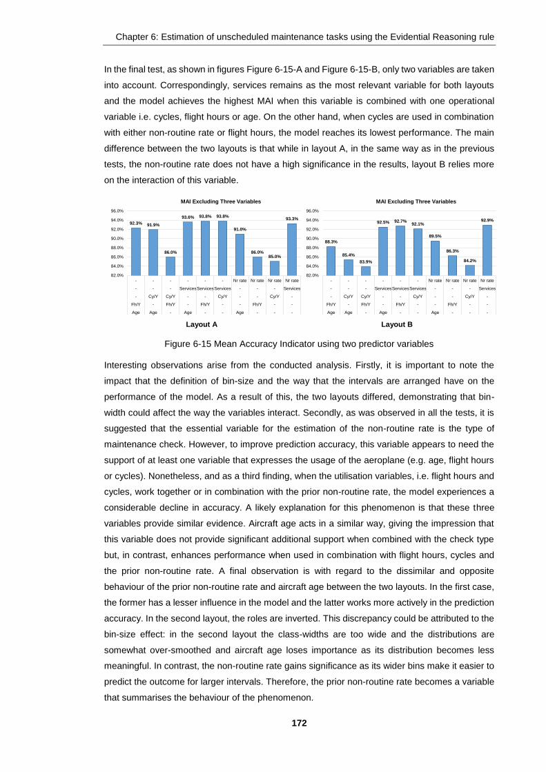
Chapter 6: Estimation of unscheduled maintenance tasks using the Evidential Reasoning rule
172
In the final test, as shown in figures Figure 6-15-A and Figure 6-15-B, only two variables are taken
into account. Correspondingly, services remains as the most relevant variable for both layouts
and the model achieves the highest MAI when this variable is combined with one operational
variable i.e. cycles, flight hours or age. On the other hand, when cycles are used in combination
with either non-routine rate or flight hours, the model reaches its lowest performance. The main
difference between the two layouts is that while in layout A, in the same way as in the previous
tests, the non-routine rate does not have a high significance in the results, layout B relies more
on the interaction of this variable.
Layout A Layout B
Figure 6-15 Mean Accuracy Indicator using two predictor variables
Interesting observations arise from the conducted analysis. Firstly, it is important to note the
impact that the definition of bin-size and the way that the intervals are arranged have on the
performance of the model. As a result of this, the two layouts differed, demonstrating that bin-
width could affect the way the variables interact. Secondly, as was observed in all the tests, it is
suggested that the essential variable for the estimation of the non-routine rate is the type of
maintenance check. However, to improve prediction accuracy, this variable appears to need the
support of at least one variable that expresses the usage of the aeroplane (e.g. age, flight hours
or cycles). Nonetheless, and as a third finding, when the utilisation variables, i.e. flight hours and
cycles, work together or in combination with the prior non-routine rate, the model experiences a
considerable decline in accuracy. A likely explanation for this phenomenon is that these three
variables provide similar evidence. Aircraft age acts in a similar way, giving the impression that
this variable does not provide significant additional support when combined with the check type
but, in contrast, enhances performance when used in combination with flight hours, cycles and
the prior non-routine rate. A final observation is with regard to the dissimilar and opposite
behaviour of the prior non-routine rate and aircraft age between the two layouts. In the first case,
the former has a lesser influence in the model and the latter works more actively in the prediction
accuracy. In the second layout, the roles are inverted. This discrepancy could be attributed to the
bin-size effect: in the second layout the class-widths are too wide and the distributions are
somewhat over-smoothed and aircraft age loses importance as its distribution becomes less
meaningful. In contrast, the non-routine rate gains significance as its wider bins make it easier to
predict the outcome for larger intervals. Therefore, the prior non-routine rate becomes a variable
that summarises the behaviour of the phenomenon.
92.3% 91.9%
86.0%
93.6% 93.8% 93.8%
91.0%
86.0%85.0%
93.3%
82.0%
84.0%
86.0%
88.0%
90.0%
92.0%
94.0%
96.0%
- - - - - - Nr rate Nr rate Nr rate Nr rate
- - - ServicesServicesServices - - - Services
- Cy/Y Cy/Y - - Cy/Y - - Cy/Y -
Fh/Y - Fh/Y - Fh/Y - - Fh/Y - -
Age Age - Age - - Age - - -
MAI Excluding Three Variables
88.3%
85.4%
83.9%
92.5% 92.7%92.1%
89.5%
86.3%
84.2%
92.9%
82.0%
84.0%
86.0%
88.0%
90.0%
92.0%
94.0%
96.0%
- - - - - - Nr rate Nr rate Nr rate Nr rate
- - - ServicesServicesServices - - - Services
- Cy/Y Cy/Y - - Cy/Y - - Cy/Y -
Fh/Y - Fh/Y - Fh/Y - - Fh/Y - -
Age Age - Age - - Age - - -
MAI Excluding Three Variables

Chapter 6: Estimation of unscheduled maintenance tasks using the Evidential Reasoning rule
173
6.5 ER rule scenarios
It is worth bearing in mind that the development of the model has followed a systematic process,
so that the results obtained in every step allow for a gradual increase in the complexity and
robustness of the model. Therefore, as already mentioned, to simplify the preceding analysis and
to have fewer variables involved, all the input variables were assumed to be completely
independent. Moreover, all pieces of evidence were assumed to be fully reliable and highly
important.
In this section, four different scenarios of the ER rule model are created using the two suggested
layouts of bin-widths and considering the five pieces of evidence. Through these scenarios, the
model continues increasing in complexity, but becomes less rigid, more meaningful and useful.
For training and validation purposes, the sample of 91 maintenance checks was randomly divided
into nine groups of ten each, keeping one extra record outside the groups. Hence, the ER model
is built considering eighty maintenance services (eight random groups of ten), and eleven (the
remaining group of ten and the extra service) are used for validation. Subsequently, the scenarios
are executed using four different samples of eighty maintenance services each, i.e. each scenario
is run eight times (four samples for each of the two interval layouts).
The first scenario is the simplest as it assumes that all the pieces of evidence are completely
independent, fully reliable and have the same importance. Nonetheless, a significant drawback is
that the model is not fully representing the actual conditions of the problem. The main
characteristic of the second scenario is that the independence of the variables can be questioned.
Therefore, the model is adjusted to assess the dependencies between the pieces of evidence,
keeping their reliability and importance as in the first scenario. In the third scenario, and taking
into account the results of the dependency assessment, the pieces of evidence are no longer
considered fully reliable. Hence, based on the specific characteristics of each variable, reliability
is adjusted, albeit the variables are still considered highly and equally important. Finally, in the
last scenario, considering the results from the former scenarios, the importance of the pieces of
evidence is reviewed and adjusted to maximise the performance of the model. To simplify the
explanation, the four scenarios are described using one sample. However, the results of the four
samples are shown for further detail in Appendix B.7 (from Table B-32 to Table B-59).
6.5.1 All pieces of evidence are independent, fully reliable and highly important
This is the basic scenario for aggregating the five predictor variables to estimate the non-routine
rate. It considers that all pieces of evidence are completely independent, fully reliable and have
the same importance; i.e. the alpha index, weight and reliability are all equal to one. Table 6-13
presents the results of this scenario for one of the samples. As already discussed, the
performance of the model is better when smaller bins are used, i.e. layout A performs better than
layout B. Contrastingly, it is interesting to discuss the MSEDIST (representing the error between
the real non-routine rate distribution and the one calculated by the model), compared with the
other indicators, which has a better result for layout B. A possible explanation for this behaviour
might be that for wider bins, the distribution smooths and therefore the error could decrease. It is

Chapter 6: Estimation of unscheduled maintenance tasks using the Evidential Reasoning rule
174
noteworthy that this scenario shows the ideal conditions for all the variables. However, this does
not fully represent the real conditions of the problem, hence, the following sections will attempt to
address this weakness.
Table 6-13 Model performance when the variables are independent, fully reliable and highly
important.
Layout A Layout B
Alpha Index 1 1
Reliability 1 1
Weight 1 1
MSEDIST 0.0128 0.0049
MSESERV 0.0005 0.0010
MAE 0.0172 0.0244
MAPE 9.28% 12.78%
MAI 95.96% 94.57%
6.5.2 All pieces of evidence are fully reliable, highly important and their
dependency is adjusted
The previous section considers that all the pieces of evidence are independent. However, in real
life, this strong assumption does not commonly occur as generally there is a certain degree of
dependency amongst the variables4. As mentioned before, Yang and Xu (2013) propose the ER
rule as a conjunctive probabilistic reasoning process for combining multiple pieces of independent
evidence. However, Yang and Xu (2015) have recently proposed a novel approach to cope with
the independency premise by including a new term in the ER rule (referred to in this study as
alpha-index) as shown in equations (4-7) and (4-8).
Analysing the dependency factor results is relevant, as considering the variables as totally
independent might lead to unrealistic results since the pieces of evidence could provide the same
information to some extent. Therefore in this section the variables are no longer considered
completely independent, although their reliability and importance remains as in the first scenario.
The dependency between the variables is adjusted by optimising the alpha-index, aiming to
represent the real relationship between the variables. Thus, an optimisation model was built
modifying the alpha-index to minimise the difference between the real non-routine rate distribution
and the distribution calculated by the model (i.e. MSEDIST). Table B-34 to Table B-57, in Appendix
B.7.1, show the optimised alpha-index values resulting from the optimisation model.
4 When two pieces of evidence are mutually exclusive, they should not be interrelated. However, if they are independent of each other, they are indeed interrelated, but conceptually their interrelationship should be such that the acquisition of one piece of evidence does not depend on whether the other piece of evidence is known or not (Yang and Xu 2013; 2015).

Chapter 6: Estimation of unscheduled maintenance tasks using the Evidential Reasoning rule
175
Table 6-14 compares the performance of the model when the variables are assumed independent
against when the dependency has been adjusted. By optimising the alpha-index the MSEDIST is
reduced to almost zero for both layouts, which means that the estimated non-routine rate
distribution is practically the same as the distribution observed in the sample. However, the other
efficiency indicators remain almost the same as in scenario 6.5.1 (with slight improvements for
layout A and minor retreats for layout B). Even though after optimising the alpha-index the overall
performance of the model was not improved considerably, the dependency amongst the variables
is now considered to closer represent the real association between the variables.
Table 6-14 Model performance when the variables are not completely independent, but are fully
reliable and highly important.
Layout A Layout B
Original Optimising
alphas Original
Optimising alphas
Alpha Index 1 Optimised 1 Optimised
Reliability 1 1 1 1
Weight 1 1 1 1
MSEDIST 0.0128 0.0000 0.0049 0.0000
MSESERV 0.0005 0.0004 0.0010 0.0010
MAE 0.0172 0.0155 0.0244 0.0240
MAPE 9.28% 8.00% 12.78% 12.89%
MAI 95.96% 96.35% 94.57% 94.67%
6.5.3 All pieces of evidence are highly important, their dependency is adjusted
and they are not fully reliable
Now that the dependency between the variables has been identified in section 6.5.2, another
characteristic of the pieces of evidence can be analysed. In this section, the variables are still
considered to be highly important, their dependency is given by the adjusted alpha-index, but they
are not considered fully reliable. Therefore, each of the pieces of evidence is studied and their
reliability is estimated based on their main features and considering their process of collection,
recording and analysis. Gathering, recording, analysis and management are relevant due to the
reliability of a piece of evidence being affected by all the elements involved in it, from the moment
the data is generated until stored and used by the model. In other words, the reliability of a piece
of evidence cannot be modified directly in the model, as it is an inherent feature of the quality of
information and only by its improvement can reliability be increased.
As explained in chapter 2, to ensure airworthiness aircraft maintenance is structured in a rigorous
system that relies heavily on accurate information. Nowadays most of the information is managed
automatically, including flight hours and cycles. However, there is still some information that is
recorded and analysed manually and this increases error margin and subjectivity, such as the
number of non-routine tasks in a maintenance service. Additionally, there is information that is

Chapter 6: Estimation of unscheduled maintenance tasks using the Evidential Reasoning rule
176
recorded automatically and is rigorously analysed, but contains some manual stages in the
management process which could lead to inaccuracies. Age and service type are part of this
cohort.
The non-routine tasks are programmed to correct the failures and discrepancies found during the
execution of the scheduled tasks. However rework-tasks (tasks to correct errors or deficiencies
in the quality) and miscellaneous activities (additional tasks not included in the plan, but necessary
to properly execute it) are also commonly registered as non-routine tasks. These extra activities
might bias the indicator of measuring the unexpected damage and failures during a maintenance
check.
According to experience, it is believed that around 5% of non-routine tasks could be rework and
miscellaneous tasks. Therefore, a reliability of 0.95 for non-routine rate is considered. Since the
non-routine rate is the outcome of the model, its reliability must be considered for the final
reliability of the predictor variables. For instance, for the non-routine rate prior distribution a
reliability of 0.90 is assumed (i.e. the reliability of the non-routine rate is considered twice, 0.95
by 0.95).
Aircraft age is measured from the aircraft's manufacturing date to the start date of the
maintenance check and this information is well registered in the maintenance records. Even so,
one inconsistency was found in one of the records, where there was a typographical error in the
fabrication year. Thus, the reliability of this variable had to be reduced to 0.95, reflecting other
possible inconsistencies. The final reliability of this variable, after including the non-routine rate
reliability, is 0.90.
Flight hours and cycles are two scrupulously managed variables as they are used for different
areas in the airline. They are recorded and analysed automatically by sensors within the aircraft.
Therefore, the quality of this piece of evidence could be considered significantly high.
Nonetheless, to reduce the correlation between total flight hours and total cycles with age, annual
utilisation was used instead. The main drawback of using this annualised value is that flight hours
and cycles per year are an average indicator of the usage of the aeroplane. Therefore, the
reliability for these two pieces of evidence is first assumed as 0.97 and then, considering the non-
routine rate reliability, as 0.92.
Maintenance service type is the essential variable for organising and managing maintenance
activities, as it is very well defined in the scheduled maintenance programme. Hence, this piece
of evidence is considered fully reliable with a final reliability value of 0.95 after including the non-
routine rate reliability.
After updating the reliability of the pieces of evidence based on the characteristics of the variables,
it can be noticed in Table 6-15 that model performance drops considerably in comparison to the
results from scenario 6.5.2. In a similar way to the adjustment of dependency, greater reliability
values might produce better efficiency results in the model. However, if these values are not
based on the real quality of the information, the model results would not be realistic. In other
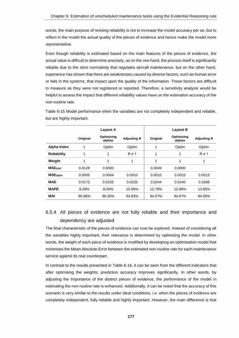
Chapter 6: Estimation of unscheduled maintenance tasks using the Evidential Reasoning rule
177
words, the main purpose of revising reliability is not to increase the model accuracy per se, but to
reflect in the model the actual quality of the pieces of evidence and hence make the model more
representative.
Even though reliability is estimated based on the main features of the pieces of evidence, the
actual value is difficult to determine precisely, as on the one hand, the process itself is significantly
reliable due to the strict normativity that regulates aircraft maintenance, but on the other hand,
experience has shown that there are weaknesses caused by diverse factors, such as human error
or fails in the systems, that impact upon the quality of the information. These factors are difficult
to measure as they were not registered or reported. Therefore, a sensitivity analysis would be
helpful to assess the impact that different reliability values have on the estimation accuracy of the
non-routine rate.
Table 6-15 Model performance when the variables are not completely independent and reliable,
but are highly important.
Layout A Layout B
Original Optimising
alphas Adjusting R Original
Optimising alphas
Adjusting R
Alpha Index 1 Optim Optim 1 Optim Optim
Reliability 1 1 R ≠ 1 1 1 R ≠ 1
Weight 1 1 1 1 1 1
MSEDIST 0.0128 0.0000 0.0049 0.0000
MSESERV 0.0005 0.0004 0.0010 0.0010 0.0010 0.0013
MAE 0.0172 0.0155 0.0220 0.0244 0.0240 0.0268
MAPE 9.28% 8.00% 10.95% 12.78% 12.89% 13.85%
MAI 95.96% 96.35% 94.83% 94.57% 94.67% 94.05%
6.5.4 All pieces of evidence are not fully reliable and their importance and
dependency are adjusted
The final characteristic of the pieces of evidence can now be explored. Instead of considering all
the variables highly important, their relevance is determined by optimising the model. In other
words, the weight of each piece of evidence is modified by developing an optimisation model that
minimises the Mean Absolute Error between the estimated non-routine rate for each maintenance
service against its real counterpart.
In contrast to the results presented in Table 6-16, it can be seen from the different indicators that
after optimising the weights, prediction accuracy improves significantly. In other words, by
adjusting the importance of the distinct pieces of evidence, the performance of the model in
estimating the non-routine rate is enhanced. Additionally, it can be noted that the accuracy of this
scenario is very similar to the results under ideal conditions, i.e. when the pieces of evidence are
completely independent, fully reliable and highly important. However, the main difference is that

Chapter 6: Estimation of unscheduled maintenance tasks using the Evidential Reasoning rule
178
in this final scenario, alpha index, reliability and weight have been adjusted to represent as close
as possible the actual conditions of the model.
Figure 6-16 illustrates the weight of each of the intervals for the different pieces of evidence for
the different samples in layouts A and B. For instance, in Figure 6-16-layout A, it can be noted
that for service type, intervals 1, 3, 6 and 9 that correspond to services 1C, 3C, 4C+ and 6
respectively have a relevant role for the estimation of non-routine rate. In contrast, the non-routine
prior distribution has almost null importance for the model. Besides, it is also important to
emphasise the noticeable similarities between the results of the different samples. Table B-58
and Table B-59, in Appendix B.7.2, present the optimised values of the weights that minimise
prediction error.
Table 6-16 Model performance when the variables are not completely independent, reliable and
important.
Layout A Layout B
Original Optimising
alphas Adjusting
R Optimising
W Original
Optimising alphas
Adjusting R
Optimising W
Alpha Index 1 Optim Optim Optim 1 Optim Optim Optim
Reliability 1 1 R ≠ 1 R ≠ 1 1 1 R ≠ 1 R ≠ 1
Weight 1 1 1 Optim 1 1 1 Optim
MSEDIST 0.0128 0.0000 0.0049 0.0000
MSESERV 0.0005 0.0004 0.0010 0.0009 0.0010 0.0010 0.0013 0.0011
MAE 0.0172 0.0155 0.0220 0.0203 0.0244 0.0240 0.0268 0.0243
MAPE 9.28% 8.00% 10.95% 10.28% 12.78% 12.89% 13.85% 12.08%
MAI 95.96% 96.35% 94.83% 95.23% 94.57% 94.67% 94.05% 94.59%
Layout A
Layout B
Figure 6-16 Importance degree (weight value) for each piece of evidence
In summary, to understand the general behaviour of the model, a simple scenario was created
assuming perfect conditions. The dependency between the variables and their reliability were
then adjusted to represent the actual characteristics of the information. Finally, the importance of
the pieces of evidence was modified to improve the estimation of non-routine rate. However, these
scenarios only show the performance for a given combination of dependency, reliability and
0.00
0.20
0.40
0.60
0.80
1.00
1 3 5 7 9 11131517 2 4 6 8 101214 1 3 5 7 9 11131517 1 3 5 7 9
Age Fh/Y Cy/Y ServicesNr rate
We
igh
t
Optimised Weight of each Piece of Evidence
Sample A Sample B Sample C Sample D
0.00
0.20
0.40
0.60
0.80
1.00
1 3 5 2 4 6 8 10 12 14 1 3 5 1 3 5 7 9
Age Fh/Y Cy/Y Services Nr rate
We
igh
t
Optimised Weight of each Piece of Evidence
Sample A Sample B Sample C Sample D

Chapter 6: Estimation of unscheduled maintenance tasks using the Evidential Reasoning rule
179
weight. Therefore, it would be useful to deeply analyse the effect of these three evidence qualities
on prediction accuracy. Hence, the next section aims to discover the aforementioned effect.
6.6 Sensitivity analysis of reliability
In addition to the scenarios presented in the section above, a sensitivity analysis was carried out
to determine how reliability, importance and dependency of the pieces of evidence might impact
upon the efficiency of estimating the non-routine rate, in other words, how a change in the values
of reliability, weight or alpha-index might lead to different performance results. Hence, several
experiments were conducted. The first assigned different reliability values to each of the predictor
variables, but considered that the alpha index had already been adjusted and that the weights
are equal to one. Secondly, the reliability of all the pieces of evidence was modified to assess
their global impact, but keeping the previous assumptions. Finally, aiming to evaluate the
influence of the dependency and relevance of the pieces of evidence, the final experiment
changed the reliability and the values of the alpha-index and the weight, assuming these last two
variables as equal to one and later using their optimised values.
All the sensitivity experiments were carried out twice for the four samples described in section
6.5, using the defined layouts A and B. For layout A, bin-widths of 0.5, 150, 100, and 0.05 for a,
fhy, cy and nrr, respectively were used and for layout B, bin-widths of 2.5, 150, 300, and 0.1 for
a, fhy, cy and nrr, each.
6.6.1 Alpha index has been optimised, weight is one and the reliability of one
piece of evidence changes.
In order to assess the influence of the reliability on model performance and to address the
relevance of each variable, in this scenario the accuracy is obtained by changing the reliability for
one piece of evidence at a time, from being completely unreliable to a full reliability, while the
other variables remain fully reliable. It also considers that the dependency of the variables has
been adjusted by optimising the alpha-index, and assumes that all pieces of evidence are highly
and equally important. Thus, the inference model is applied several times, changing in each round
the reliability value of one variable from 0 to 1, considering the alpha index obtained in section
6.5.2. Weights are equal to 1. This process is repeated for every variable.
Figure 6-17 shows model accuracy when the reliability of one piece of evidence is changed in a
range from 0 to 1, for layout A and B respectively. Each curve represents the behaviour of a
specific variable towards a variation in the reliability value. From these figures, it can be observed,
in both layouts, the remarkable sensitivity of the model towards changes in the reliability of the
maintenance service type, emphasising with this the relevant role that this piece of evidence has
on the estimation of the non-routine rate. In both layouts, it can be seen that when the reliability
of the service type is low, the accuracy of the model is significantly lower too. On the other hand,
when reliability increases, the performance of the model soars as well, showing a steady
increment until the reliability almost reaches a value of 0.9, when it increases dramatically. It is
noteworthy that the influence of this variable is more evident in layout B. Model performance is

Chapter 6: Estimation of unscheduled maintenance tasks using the Evidential Reasoning rule
180
also sensitive to variations in the reliability of flight hours per year, meaning that the absence of
this variable or its lack of reliability can impact considerably upon prediction accuracy. However,
in layout B this sensitivity is not as pronounced as in layout A.
Estimation of the non-routine rate is less sensitive to changes in the reliability of the remaining
three variables, as their fluctuations do not appear to have great effect on the results.
Nonetheless, it is interesting that their role level is not the same between both layouts. For
instance, cycles in layout A still have considerable repercussions for accuracy, while for layout B
the prediction of the non-routine rate is almost neutral to changes to the cycles’ reliability.
Meanwhile, variations in the reliability for age and non-routine rate do not have a significant impact
on the prediction accuracy for layout A whereas they still show an influence in layout B.
Figure 6-17 presents the behaviour for one of the samples analysed. The detailed results from
this sensitivity test for the four samples along with their corresponding graphs are presented in
Appendix B.8.1 (from Table B-60 to Table B-69). It is worth mentioning that the outcomes of the
four samples are similar.
Layout A Layout B
Figure 6-17 Model sensitivity when the reliability of one variable is modified, for layouts A and B
In summary, the results of this sensitivity test reinforce what was observed in the analysis
presented in section 6.4.2, where it was concluded that maintenance service type is an essential
piece of evidence for the estimation of the non-routine rate, followed by flight hours per year.
Moreover, in order to have a higher accuracy prediction, these two variables have to be
considered in the model, but also should be highly reliable. In addition to the outcomes of this
test, it is necessary to analyse the global effect that the five variables have on the model efficiency.
This analysis is carried out in the next section.
6.6.2 Alpha index has been optimised, weight is one and reliability is the same
for all pieces of evidence.
This sensitivity test also aims to analyse the effect of reliability on model performance, but also
considering the impact of all pieces of evidence as a whole. Hence, this scenario assumes that
all the variables have the same reliability value, i.e. all of them are equally reliable, and this
increases the global value from being completely unreliable to highly reliable. In other words, the
ER model is run several times using the alpha index calculated in section 6.5.2; weights equal to
1, and reliability in all the variables growing from 0 to 1 in each run.
91.5%
92.5%
93.5%
94.5%
95.5%
96.5%
0 0.1 0.2 0.3 0.4 0.5 0.6 0.7 0.8 0.9 1
MA
I
Reliability
Mean Accuracy Indicator per Variable
Age
Fh/y
Cy/y
Services
NRR
91.5%
92.5%
93.5%
94.5%
95.5%
96.5%
0 0.1 0.2 0.3 0.4 0.5 0.6 0.7 0.8 0.9 1
MA
I
Reliability
Mean Accuracy Indicator per Variable
Age
Fh/y
Cy/y
Services
NRR

Chapter 6: Estimation of unscheduled maintenance tasks using the Evidential Reasoning rule
181
Figure 6-18 illustrates model accuracy when the reliability of all pieces of evidence varies equally.
The behaviour of the four analysed samples is presented to show that both layouts have very
similar patterns. The detailed results of this sensitivity test are presented in Appendix B.8.2 (from
Table B-70 to Table B-72). From the figures, it can be noted that when the reliability of all pieces
of evidence is almost null, the prediction accuracy of the model reaches its lowest value for both
layouts, near 91%. In contrast, when reliability grows, the model performance is enhanced.
However this improvement is considerably better for layout A in comparison to layout B, especially
when it is closer to being fully reliable. Accuracy rises significantly, achieving almost 97%. In
contrast, for layout B the increment is less noteworthy, rising to less than 95%. These results
confirm that the layout with smaller bins has a better performance and strengthen the idea that
layout A is more sensitive to changes in the reliability of the pieces of evidence.
After a comparison between the lowest global accuracy value (91% for both layouts) obtained in
this test, against the lowest efficiency values from the experiment presented above (around 94.5%
for layout A and less than 92% for layout B), it is interesting to note that in layout B the values are
significantly close, which might suggest that for this layout the service type is the evidence that
provides almost all of the information for estimating the non-routine rate.
Layout A
Layout B
Figure 6-18 Model sensitivity when the reliability of all variables is modified, for layouts A and B
In the two sensitivity experiments described above, reliability was the main component analysed.
Nonetheless, it is also necessary to explore the effect that dependency and weight have on
prediction accuracy. Therefore, the following tests attempt to study the influence of these two
components.
6.6.3 Reliability is the same for all pieces of evidence, weight and Alpha index
are equal to one and then optimised.
The following sensitivity tests consider the variables equally reliable and increasing its value in
each iteration, similarly as in the previous analysis. However, the tests are more comprehensive,
considering also the effect of alpha-index and weights in model efficiency. In order to study these
conditions, four different experiments were developed. The first two assume that all the pieces of
evidence are completely independent. One test considers that all pieces of evidence are highly
and equally important, while the other optimises the weights to reduce the prediction error. The
remaining two experiments are based on the same weight scenarios, but use the adjusted
dependency index. Summarising, one case considers alpha index and weight equal to one and
90%
91%
92%
93%
94%
95%
96%
97%
0 0.1 0.2 0.3 0.4 0.5 0.6 0.7 0.8 0.9 1
MA
I
Reliability
Mean Accuracy Indicator Vs Reliablity
Sample A
Sample B
Sample C
Sample D
90%
91%
92%
93%
94%
95%
96%
97%
0 0.1 0.2 0.3 0.4 0.5 0.6 0.7 0.8 0.9 1
MA
I
Reliability
Mean Accuracy Indicator Vs Reliability
Sample A
Sample B
Sample C
Sample D

Chapter 6: Estimation of unscheduled maintenance tasks using the Evidential Reasoning rule
182
the second assumes alpha index is one while the weight is optimised. In the third, alpha index is
optimised and weight is equal to one and in the fourth, both alpha index and weight are optimised.
For the four scenarios the model is run several times changing the reliability value from 0 to 1 for
all the variables. The results of these tests are described using one of the samples and the
detailed results for the four samples are presented along with their graphs in Appendix B.8.3 (from
Table B-73 to Table B-82).
Considering a specific reliability, these four sensitivity experiments are created firstly, to assess
the impact that optimising the weights might have on model performance by contrasting these
results against accuracy when the weights are assumed to be equal to one and secondly, to
compare the behaviour of the model when it is assumed that the variables are completely
independent in contrast to when dependency has been adjusted by optimising the alpha-index
values.
Figure 6-19 presents the case when it is assumed that all the pieces of evidence are completely
independent, comparing the accuracy when the variables are considered highly important against
the results when the importance has been adjusted, i.e. mathematically expressed as alpha index
equal to one, weight equal to one for one of the curves and optimised for the other.
For both layouts, when the pieces of evidence are assumed to be completely independent and
highly important (alpha-index = 1 and weight = 1), the model behaves in the same way as has
already been explained. For inferior reliability values, the accuracy of the model is also low and
when reliability increases, performance is also boosted but to a higher degree. However, when
the importance of the pieces of evidence is adjusted to minimise the prediction error, the accuracy
of the model enhances dramatically, even when the variables are considered unreliable.
Nevertheless, it can be noted that this level of efficiency remains practically stable to changes in
reliability, unless the variables are almost fully reliable where the model reaches its maximum
accuracy point. Additionally, it appears that the optimisation of the weights can compensate for
the lack of reliability of the variables by adjusting the importance of the pieces of evidence to
obtain better accuracy results.
Layout A
Layout B
Figure 6-19 Model sensitivity when α=1, the reliability of all variables is modified and weight is
optimised, for layouts A and B
90%
91%
92%
93%
94%
95%
96%
97%
0 0.1 0.2 0.3 0.4 0.5 0.6 0.7 0.8 0.9 1
MA
I
Reliability
MAI vs ReliabilityAlpha=1
Weight=1 and Optimised
Alpha = 1, W = 1 Alpha = 1, W = Optimised
90%
91%
92%
93%
94%
95%
96%
97%
0 0.1 0.2 0.3 0.4 0.5 0.6 0.7 0.8 0.9 1
MA
I
Reliability
MAI vs ReliabilityAlpha=1
Weight=1 and Optimised
Alpha = 1, W = 1 Alpha = 1, W = Optimised

Chapter 6: Estimation of unscheduled maintenance tasks using the Evidential Reasoning rule
183
Figure 6-20 compares the weights in the same way as in Figure 6-19, obtaining very similar
results. The difference is that, for this case, dependency between the variables has been adjusted
by optimising the alpha index. In this case, it can also be observed that the performance of the
model is improved considerably by optimising the weights. Nevertheless, it seems that there is
an upper limit of improvement that cannot be gone beyond by only adjusting the weights. To go
further than that efficiency limit and enhance model performance, it is necessary to increase the
reliability of the variables, i.e. improve the quality of the information.
Layout A
Layout B
Figure 6-20 Model sensitivity when α has been adjusted, the reliability of all variables is
modified and weight is optimised, for layouts A and B
Figure 6-21 compares the two cases described above where it can be observed that, for reliability
values up to approximately 0.8, the model has a higher accuracy when the variables are assumed
to be independent in comparison to when the dependency has been adjusted. However, this
difference is more noticeable when the weight of the pieces of evidence is equal to one. It is only
when the variables are almost fully reliable that this pattern is inverted, i.e. for higher reliability
values, the prediction accuracy is better when the alpha index has been optimised. A possible
explanation of this phenomenon could be that assuming the independence of the pieces of
evidence might somehow duplicate or overlap the information provided by the pieces of evidence.
Another interesting finding is that the performance of the model once the weights have been
optimised is very similar, either when the alpha index is one or when it has been optimised,
suggesting that this is the maximum accuracy level that can be reached by adjusting the
importance of the pieces of evidence, i.e. by optimising the weights.
91%
92%
93%
94%
95%
96%
97%
0 0.1 0.2 0.3 0.4 0.5 0.6 0.7 0.8 0.9 1
MA
I
Reliability
MAI vs ReliabilityAlpha Optimised
Weight=1 and Optimised
Alpha = Optimised, W = 1 Alpha = Optimised, W = Optimised
91%
92%
93%
94%
95%
96%
97%
0 0.1 0.2 0.3 0.4 0.5 0.6 0.7 0.8 0.9 1
MA
I
Reliability
MAI vs ReliabilityAlpha Optimised
Weight=1 and Optimised
Alpha = Optimised, W = 1 Alpha = Optimised, W = Optimised

Chapter 6: Estimation of unscheduled maintenance tasks using the Evidential Reasoning rule
184
Layout A Layout B
Figure 6-21 Model sensitivity comparison when α=1 and then is adjusted, and when weight=1
and then is optimised, for layouts A and B
Finally, it is interesting to observe in detail how the importance of the variables is adjusted for
different reliability values. Each line in Figure 6-22 A, B, C and D represent the optimised weight
for each interval of the input variables given a particular reliability (Figure A and D depict the
weights for layout A when alpha index is one and when it has been optimised, respectively.
Figures B and D are similar, but based on layout B). Interestingly, as can be seen in the figures,
the values of the weight are very similar for the different reliability values (i.e. the lines are
practically overlapping each other), with the exception of when reliability is 0.9. This might suggest
that with small changes in the weight values, the model is capable of adjusting and maintaining
accuracy for different reliability values. However, for higher reliability values, when the accuracy
starts reaching its maximum value the changes in the weight are more remarkable, possibly as a
result of the enhancement of accuracy.
Layout A Layout B
A) B)
90%
91%
92%
93%
94%
95%
96%
97%
0 0.1 0.2 0.3 0.4 0.5 0.6 0.7 0.8 0.9 1
MA
I
Reliability
MAI vs ReliabilityAlpha=1 and OptimisedWeight=1 and Optimised
Alpha = Optimised, W = 1 Alpha = Optimised, W = Optimised
Alpha = 1, W = 1 Alpha = 1, W = Optimised
90%
91%
92%
93%
94%
95%
96%
97%
0 0.1 0.2 0.3 0.4 0.5 0.6 0.7 0.8 0.9 1
MA
I
Reliability
MAI vs ReliabilityAlpha=1 and OptimisedWeight=1 and Optimised
Alpha = Optimised, W = 1 Alpha = Optimised, W = Optimised
Alpha = 1, W = 1 Alpha = 1, W = Optimised
0.0
0.1
0.2
0.3
0.4
0.5
0.6
0.7
0.8
0.9
1.0
1 3 5 7 9 11131517 2 4 6 8 101214 1 3 5 7 9 11131517 1 3 5 7 9
Age Fh/Y Cy/Y Services Nrrate
Weig
ht
Intervals of each Variable
Optimised Weight for Different Reliability Values (α=1)
r = 0.0 r = 0.1 r = 0.2 r = 0.3 r = 0.4
r = 0.5 r = 0.6 r = 0.7 r = 0.8 r = 0.9
0.0
0.1
0.2
0.3
0.4
0.5
0.6
0.7
0.8
0.9
1.0
1 3 5 2 4 6 8 10 12 14 1 3 5 1 3 5 7 9
Age Fh/Y Cy/Y Services Nr rate
Weig
ht
Intervals of each Variable
Optimised Weight for Different Reliability Values (α=1)
r = 0.0 r = 0.1 r = 0.2 r = 0.3 r = 0.4
r = 0.5 r = 0.6 r = 0.7 r = 0.8 r = 0.9

Chapter 6: Estimation of unscheduled maintenance tasks using the Evidential Reasoning rule
185
C)
D)
Figure 6-22 Importance degree (optimised weight values) for each piece of evidence for
different reliability values, for layouts A and B
As this inference model is based on a small sample, the results from the sensitivity experiments
cannot be considered as conclusive and therefore should not be used to generalise the behaviour
of other ER models. Nevertheless, the presented sensitivity experiments were useful to gain
insight into the influence that the reliability, dependency and importance of the pieces of evidence
have on model performance. Firstly, they allow visualisation of the role that each of the variables
have in prediction accuracy, which supports the idea that maintenance service type is a
fundamental piece of evidence for this model. Secondly, it has been shown that for higher
reliability values, the model performs considerably better. However, reliability cannot be modified
directly and it is only when the quality of the information is improved that the reliability of a piece
of evidence would increase. Thirdly, even when the accuracy of the model might be lower when
the dependency of the pieces of evidence has been adjusted, this would offer a more
representative model, abstracting reality in a better way. Finally, adjusting the importance of the
pieces of evidence might lead to better prediction results. However, it is important to mention that
there is a maximum limit for this improvement as a result of this modification. It is noteworthy that
modifying or adjusting these features must be done with caution as increasing accuracy is not the
only aim that should be taken into account. It is also important to consider the representativeness
of these variables and the meaningfulness of the model.
6.7 Validation
As explained in section 6.5, from the original database of 91 maintenance checks, four different
samples of 80 random maintenance services were used to build the model and the remaining
eleven of each sample were used for validation purposes. The model was run on the validation
group using the adjusted values for alpha index, reliability and weight obtained in sections 6.5.2,
6.5.3 and 6.5.4. Figure 6-23 compares the performance of the model for the training group, the
validation fragment and also for the whole sample. Here, it can be seen that overall model
performance is lower in the validation sample. However, the efficiency of the model is still
satisfactory, as evidenced by the MAI values. For layout A, the accuracy for training is around
96% whilst accuracy for the validation fragment ranges from 90% to 94%. For layout B the
0.0
0.1
0.2
0.3
0.4
0.5
0.6
0.7
0.8
0.9
1.0
1 3 5 7 9 11131517 2 4 6 8 101214 1 3 5 7 9 11131517 1 3 5 7 9
Age Fh/Y Cy/Y Services Nrrate
Weig
ht
Intervals of each Variable
Optimised Weight for Different Reliability Values (α Optimised)
r = 0.0 r = 0.1 r = 0.2 r = 0.3 r = 0.4
r = 0.5 r = 0.6 r = 0.7 r = 0.8 r = 0.9
0.0
0.1
0.2
0.3
0.4
0.5
0.6
0.7
0.8
0.9
1.0
1 3 5 2 4 6 8 10 12 14 1 3 5 1 3 5 7 9
Age Fh/Y Cy/Y Services Nr rate
Weig
ht
Intervals of each Variable
Optimised Weight for Different Reliability Values (α Optimised)
r = 0.0 r = 0.1 r = 0.2 r = 0.3 r = 0.4
r = 0.5 r = 0.6 r = 0.7 r = 0.8 r = 0.9

Chapter 6: Estimation of unscheduled maintenance tasks using the Evidential Reasoning rule
186
accuracy for training is approximately 95%, whilst the validation accuracy varies from 90% to
95%. In other words, the ability of the model to estimate the non-routine rate is remarkable for
both arrays of bins. The complete performance results are presented in Table B-83 and Table
B-84 in Appendix B.9.
Layout A
Layout B
Figure 6-23 MAI comparison for training and validation groups and for the whole sample
As part of the validation stage, the model estimates the non-routine rate given particular
operational and maintenance characteristics of the aeroplane, i.e. for an aeroplane with a specific
age, flight hours and cycles per year, which will undergo certain maintenance service, the model
estimates the non-routine rate based on the knowledge acquired during the training process.
There are three possible ways in which the model can estimate the non-routine rate. Firstly, if the
combination of maintenance and operational characteristics are already in the knowledge base,
the model simply searches for the non-routine rate value of this specific arrangement and assigns
it to the required combination. Secondly, if the combination is not in the original database but the
particular pieces of evidence are available, the model estimates the non-routine rate based on
the knowledge from the training phase, using the belief distributions, alpha-index, reliability and
weight values. If the model does not have information about the qualities of the pieces of evidence
(alpha-index, reliability and weight), it assumes the ideal case, i.e. completely independent, fully
reliable and highly important, as appropriate. Finally, when one of the pieces of evidence needed
to estimate the non-routine rate is not available in the knowledge database, the non-routine rate
is calculated based on the information provided by the remaining pieces of evidence. It is worth
noting that this prediction is considerably less accurate compared with that obtained using the
complete information.
Despite the satisfactory results from validation, the model is not as accurate as it might be as the
sample used to build the knowledge base is limited and small. Likewise, it is believed that a larger
sample might have better estimation results. Moreover, the model is able to grow in knowledge
and precision with every new addition to the sample, i.e. every new maintenance service that is
appended to the database, and this would help to enrich the information and improve estimation
accuracy.
95.2%96.1% 96.4%
95.9%
91.6%
90.3% 89.9%
94.4% 94.8%95.4% 95.6% 95.7%
86.0%
88.0%
90.0%
92.0%
94.0%
96.0%
98.0%
S1 S2 S3 S4 S1 S2 S3 S4 S1 S2 S3 S4
Training Validation All
MAI of Training, Validation and All Data-points
94.6%
95.7% 95.6% 95.4%94.8%
91.7%
90.1%
93.0%
94.6%95.2% 94.9% 95.1%
86.0%
88.0%
90.0%
92.0%
94.0%
96.0%
98.0%
S1 S2 S3 S4 S1 S2 S3 S4 S1 S2 S3 S4
Training Validation All
MAI of Training, Validation and All Data-points

Chapter 6: Estimation of unscheduled maintenance tasks using the Evidential Reasoning rule
187
6.8 Summary
The proposed model presents an innovative way for estimating non-routine rate in aircraft
maintenance services based on the evidential reasoning rule, by using different but
complementary pieces of evidence (aeroplane age, flight hours and cycles per year, service type
and the non-routine rate of the whole sample). The model is used to estimate the unscheduled
tasks that arise from unexpected damage and discrepancies. These unplanned additional tasks
might alter the original plan, hindering its daily control, causing delays, overrunning costs and
even risking the quality of the service. Therefore, the estimation of non-routine tasks might be
useful for airlines and MROs to programme activities and to plan and allocate resources
efficiently.
In this chapter, the effect on prediction accuracy of changing the interval size and the position of
its limits, but also the impact of using a different arrangement of intervals amongst the variables,
was explored. As a result of this analysis, it was found that, in general, the smaller the bins and
the lesser the intervals, the better the estimation accuracy. Additionally, choosing the appropriate
interval limits and the proper arrangement of classes between the variables might lead to better
estimation of non-routine rate.
Furthermore, the influence that each of the different variables has on model performance was
analysed. Firstly, it was noted that the arrangement of bin size could affect the way the variables
interact, changing their importance in the model. Secondly, it appears that maintenance service
type is the most relevant variable for the prediction of the non-routine rate, but to enhance model
efficiency, this variable requires the support of at least one variable that describes aircraft
utilisation (age, flight hours or cycles). Thirdly, it seems that some variables provide similar
evidence for the estimation of non-routine tasks and hence, when they are combined, the model
accuracy drops considerably. In contrast, when the variables are aggregated to others that
provide supplementary information, prediction accuracy increases. Additionally, it was observed
that when an array of small bins is chosen, the influence that the prior non-routine rate has on
prediction accuracy is insignificant. Contrastingly, when larger bins are used, the role of this
variable increases considerably.
Four scenarios were built to improve model accuracy, but more importantly its representativeness,
by adjusting the qualities of the information. In the first scenario, dependency was modified by
optimising the alpha-index. Then, in the second scenario, the reliability of the pieces of evidence
was altered to represent the quality of the information. The main aim of these two scenarios was
to shape the model to resemble reality as closely as possible. Finally, in the last scenario, the
weights were optimised by regulating the importance of the pieces of evidence to enhance model
performance.
In this chapter, different sensitivity experiments were carried out to analyse how the model reacts
to changes in specific qualities of the information. First of all, the reliability of one variable was
modified at a time, while the others remained fully reliable. Here, the service type emerged as the
variable that most influenced the model, reinforcing former observations. Then, a second

Chapter 6: Estimation of unscheduled maintenance tasks using the Evidential Reasoning rule
188
experiment was performed to analyse the global sensitivity of the model towards changes in
reliability, showing that for greater reliability values the prediction accuracy improves dramatically.
For the last experiment, not just reliability was modified, but also dependency and weights. It was
found that prediction accuracy is slightly better when the pieces of evidence are assumed to be
independent compared to when dependency has been adjusted. Moreover, when the weights are
optimised, accuracy increases considerably even for lower reliability values, reaching a ceiling of
performance.
After fine-tuning the model by modifying the alpha index, reliability and weights and analysing the
sensitivity of the model towards changes in these parameters, it was necessary to test the real
capacity of the model to estimate the non-routine rate. Thus, using the information and knowledge
acquired from the training data, the model was used to estimate the non-routine rate from a
different sample. The results were evaluated and compared against the performance from the
training data. In general the model estimation accuracy shows satisfactory results having a MAI
around 90% to 95%. It is believed that the model performance can improve if a larger sample of
maintenance services is used. However, as described in the validation section, by adding each
new maintenance service to the existing database, the model will adjust increasing in knowledge
and precision.
189
Chapter 7: Discussion and conclusions
The main research goal was to analyse the effect of unscheduled maintenance tasks on the
occurrence of delays and disruptions during the execution of aircraft heavy maintenance services.
In order to achieve this objective, an exploratory case study was carried out based on empirical
knowledge about the problem, supported by an extensive literature review and using real
operational and maintenance records from an airline.
This final chapter aims to compile and discuss the main findings and results obtained throughout
the development of this research as described in the previous chapters. Firstly, a summary of the
empirical and theoretical bases of the problem is presented. The modelling process for building
the system dynamics and the evidential reasoning rule models is then briefly described. After that,
the research findings are discussed, linking them to the research questions. The main research
limitations are examined next, followed by some suggestions for possible future research. Finally,
the general conclusions of this research are presented.
7.1 Empirical and theoretical grounding
The airline industry is undoubtedly fascinating for its evident capacity to interconnect places and
transport customers and goods and particularly because of its important role in globalisation,
economic growth and social development. It is a very competitive and dynamic industry,
characterised by large revenues and low-profit margins. In order to subsist in this hostile market,
airlines and MROs are forced to implement strategies that improve their financial performance
without compromising service quality. Some of the strategies have focused on aircraft
maintenance as this is one of the main operating costs, having also great relevance for safety
and service quality.
The maintenance of an aircraft is an unavoidable duty, organised in a systematic programme of
scheduled tasks that is defined in conjunction with aviation authorities and manufacturers, and
customised by airlines. Its key objective is to ensure the safety of aeroplane operations. It should
be performed at the lowest possible cost with the highest quality standards to minimise impact on
airline performance. Aircraft maintenance is grouped in a series of service checks organised by
workload and periodicity, from the lighter and most frequent, commonly known as line
maintenance, to the most exhaustive and less frequent, called heavy maintenance.
The literature suggests that heavy maintenance is one of the most critical processes within aircraft
maintenance, where an aeroplane is out of service during a long period of time in order that a
large number of tasks requiring also a great amount of specialised resources can be performed.
Even when the tasks of the heavy maintenance check are rigorously defined in the scheduled
maintenance programme, unexpected damage and failures are common occurrences and
unscheduled activities must be performed to deal with these eventualities. These additional

Chapter 7: Discussion and conclusions
190
activities might have great impact on the overall schedule, leading to disruptions of the process
and affecting delivery time and cost.
Specifically, as borne out both by personal experience and the literature review, the problem is
the stochastic nature of non-routine tasks, hampering accurate planning and resource forecasts,
triggering a complex interaction between scheduled and unscheduled tasks which are in a
constant battle for resources. Therefore, due to continuous adjustments to the initial maintenance
plan, managing the heavy maintenance process is not only challenging but may impact on
scheduled times, cost and even service quality.
Due to its relevance for airlines, maintenance has been a common subject of study for many
researchers. As the line maintenance process is directly linked to daily operations, it has been a
preponderant topic of these studies, for example, to analyse workforce allocation and propose
methods to recover from disruptions. Regarding heavy maintenance, valuable proposals have
been made to address long-term planning of maintenance services and the scheduling of the
maintenance tasks within this service. However, little attention has been given to the uncertainty
caused by unscheduled maintenance tasks, assuming a predetermined tentative number of non-
routine tasks.
Due to the aforementioned characteristics, some authors have defined Heavy Maintenance as a
large, sophisticated and dynamic project. These features are normally related to the term complex
project. However, even though the concept is widely used in the literature, few studies offer a
precise definition, being frequently assumed as a synonym of a large project. After reviewing
different interpretations, it can be claimed that complex projects are very dynamic, considering a
great number of interconnected elements and activities, which are constrained in time and
resources and where uncertainty exists throughout the whole process. Therefore, in summary it
can be argued that Heavy Maintenance is a complex project.
Several authors argue that conventional project management tools by themselves fail to properly
deal with the uncertainty and dynamism of complex projects, resulting in frequent cost overrun
and missing deadlines. To overcome the limitations of the traditional methods, two main strands
have been used as alternative and supportive approaches: mathematical optimisation models
and modelling simulation. The former has been utilised to produce initial project plans that aim to
optimise the duration of activities and improve resource allocation and usage, generating more
accurate and robust project schedules. Unexpected events are normally tackled by buffering the
project budget, resources or duration, taking into account statistical information and assuming
probability distributions. Simulation has been widely applied to describe the dynamic behaviour
of a project throughout time, to explore and analyse how the project responds to certain changes
or unexpected events and to design and evaluate scenarios that improve project performance.
Given the characteristics of Heavy Maintenance and its major challenges, simulation appears as
a suitable supportive approach for representing the dynamic behaviour and the complex
interaction between its elements.

Chapter 7: Discussion and conclusions
191
Discrete Event Simulation (DES) and System Dynamics (SD) are the two main simulation
approaches that have traditionally been used to study complex projects. DES is a stochastic
modelling method that represents the transition of individual entities throughout a network of
queues and activities, evaluated in discrete asynchronous periods of time (known as events) and
where complexity arises from the randomness present in the system. DES allows a “microscopic”
perspective of the system and has the ability to model with great detail each of the elements and
their changes through time. For these reasons, DES has mainly been applied at operational and
tactical levels for analysing system performance in detail. However, to achieve the expected
results, DES requires large amounts of data and its outcome could be an extremely complicated
model for large systems. System Dynamics is a deterministic simulation approach, where the
system is represented as an array of interconnected stocks and flows modelled in small
continuous time steps (known as dt). It takes a holistic perspective of the problem, with an “aerial”
point of view of the system, emphasising that complexity arises from the feedback structure and
the dynamic interrelationship between the elements. It is frequently utilised at strategic level as a
decision support tool. Contrary to DES, SD models do not require a large amount of data and are
able to handle qualitative and quantitative information. However, their interpretation and validation
could be difficult and highly subjective. In particular, SD has proven its usefulness in project
management for understanding and analysing complex projects through its capability to represent
and model the dynamic behaviour of the system along with its sophisticated feedback structure.
Considering that heavy maintenance is a dynamic and complex project, restricted in time and
budget, where a large amount of specialised resources are required to carry out a vast number
of maintenance tasks, it would be difficult to collect detailed information of all the tasks and
resources. It was found that a systemic vision of the process was more suitable for the purpose
of this research, focussing on understanding the behaviour and feedback structure rather than an
exhaustive description of the system and its elements. Therefore, System Dynamics was
suggested as a methodology to study the heavy maintenance process and its main challenges.
However, the literature has pointed out the limitations of SD to cope with uncertainty, which is a
basic characteristic of complex projects and is also a very relevant feature within heavy
maintenance processes. Therefore, it was necessary to explore methodologies to supplement SD
and overcome this limitation.
The uncertainty of an unexpected event, happening either before or during the execution of a
project, and its associated consequences are the two key components of risk. For heavy
maintenance, risk can be seen as the uncertainty derived from the latent occurrence of
unexpected damage and failures, and the effect and severity of these events, which may affect
the performance of the maintenance process.
Uncertainty refers to a deficiency, ambiguity or absence of information, knowledge or
understanding about a particular situation and its possible outcomes. Uncertainty can be
understood, managed, and even reduced, but cannot be completely eradicated. In the execution
of a complex project there are different degrees of uncertainty depending on the availability of

Chapter 7: Discussion and conclusions
192
information and the knowledge about the system. In particular, for heavy maintenance it is difficult
to objectively know the probability distribution of the unscheduled maintenance tasks. Most of the
time, they are estimated based on subjective judgements.
Diverse theories have emerged to study uncertainty from different perspectives rather than the
traditional probabilistic approach. These theories address particular aspects of uncertainty. Fuzzy
set theory has been proposed to deal with vagueness of information, while evidence theory
focusses on information ambiguity, formed by conflict and imprecision. Given highly regulated
and strict conditions in which heavy maintenance is carried out, vagueness is not the most
relevant quality of uncertainty, but it can be argued that there could be ambiguity in information.
Therefore, the evidence theory seemed an appropriate perspective for analysing the uncertainty
of unscheduled maintenance tasks. The core of evidence theory is Dempster’s rule for combining
independent pieces of evidence. However, several authors have stressed its counter-intuitive
results when working in conflicting conditions. The evidential reasoning (ER) rule has been
proposed as a generalised conjunctive probabilistic reasoning process for combining independent
pieces of evidence, taking into account their weights and reliabilities, being capable of working
under highly or completely conflicting conditions.
To complement the SD model that analyses the dynamic behaviour of and complex interaction
between scheduled and unscheduled tasks, it was proposed to use the ER rule as a rigorous
method capable of coping with variability and ambiguity for estimating the expected number of
non-routine tasks considering their relationship with several operational and maintenance
variables.
7.2 Models summary
The SD model was used to study how complex interaction between scheduled and unscheduled
tasks hinders resource allocation during the execution of maintenance services, which might lead
to delays and disruptions. The model was built using Vensim 6.3D for the causal loop diagrams
and iThink 10.0.2 for the stock and flow diagrams, and for the mathematical modelling.
Qualitative and quantitative data were used for building the SD model. Based on the author’s
experience, an initial causal loop diagram depicting the problem was defined and after several
discussions and feedback meetings with experts, it was improved and refined. In addition, real
maintenance records considering maintenance services, time duration, number of tasks and man
hours were utilised for developing stock and flow diagrams and for building the mathematical
model.
Firstly, the conceptual model was developed by building several causal loop diagrams for
understanding and describing the factors that cause delays during the execution of heavy
maintenance services. The diagram depicts the management of scheduled task execution to
ensure that the maintenance service is carried out according to the plan and illustrates the
occurrence, evaluation and programming of unscheduled maintenance tasks, highlighting
possible causes. The execution of unscheduled maintenance tasks is represented, emphasising

Chapter 7: Discussion and conclusions
193
the resulting conflict regarding resource allocation between the two different types of tasks. When
the available resources are not sufficient to fulfil the project requirements, additional resources
are requested, the last option being an extension of the maintenance service. The model also
describes the delays in decision-making and the different attitudes taken by managers during the
execution of the maintenance service.
The conceptual model was then transformed into a quantitative SD model. Due to the limited time
frame of this research, only the workforce was analysed as the main resource of the system. The
workforce is the most complex resource to manage during the process and with the most
implications for the service. Therefore, the quantitative model remained representative and
significant but simple at the same time. Two different models were developed. The first model
explains and explores the impact of the occurrence and discovery of discrepancies on the
maintenance service duration and the effect of resource allocation on the performance of the
project. The second model describes and analyses the effect of delays on decision-making and
also on the perceptions and attitudes of decision makers towards certain aspects of the project,
for instance, backlog perception or allocation of additional labour. The two models were used to
experiment and test different maintenance policies.
The ER rule was used to develop a novel approach for estimating non-routine tasks based on
historical data regarding the usage and maintenance of an aircraft. The model was built using
MATLAB R2015a to reduce calculation time and to make the model more robust and flexible.
Using real operational and maintenance records of an airline, four variables were identified as
significant to estimate unscheduled maintenance tasks. Age, flight hours per year, cycles per year
and the type of maintenance service to execute were chosen due to their relevance for defining
and managing the maintenance programme and their relationship to the occurrence and
discovery of damage, and failures. In addition to these four variables, the distribution of non-
routine tasks in the sample of maintenance services analysed was used as further evidence to
estimate unscheduled tasks. The non-routine rate was proposed as an indicator to measure the
number of unscheduled tasks against the number of scheduled tasks and was used in the model
to describe the expected number of unplanned tasks.
The continuous variables were discretised into different equal-size intervals to facilitate both the
modelling process and interpretation for decision makers. To determine the most appropriate bin-
widths, different discretisation rules were used, considering the usefulness for practitioners and
the shape of the distributions. Once the data was discretised, the ER rule was applied recursively
to aggregate each of the pieces of evidence to estimate the expected non-routine rate of an
aeroplane undertaking a maintenance check.
Analysis was carried out to explore the effect that the class size, the position of the interval limits
and the combination of different interval arrays have on the model prediction accuracy. After the
analysis, two different arrays of intervals were chosen to conduct further experiments. In order to
evaluate the role that each of the variables played in the model performance, different scenarios
were executed varying the number and combination of variables.

Chapter 7: Discussion and conclusions
194
Based on the results of the previous analyses, four different scenarios were developed to improve
the robustness and meaningfulness of the inference model. The first scenario assumed ideal
conditions by considering that all pieces of evidence are completely independent, fully reliable
and have the same importance. Then, assuming reliability and importance as in the previous
case, the dependency between the pieces of evidence was adjusted. In the third scenario, using
the dependency values of the previous step, the reliability of the different variables was adapted
by considering their characteristics while they were still assumed to be highly and equally
important. Finally, using all the previous results, the importance of the pieces of evidence was
modified to enhance model performance in the last scenario.
Several sensitivity analyses were performed to explore how changes in the reliability, importance
and dependency of the pieces of evidence might influence the efficiency of estimating the non-
routine rate. A small sample not used in the training process was utilised to test the estimation
accuracy of the model.
7.3 Research findings
Four research questions were proposed to address particular aspects of the problem. The first
two questions were answered by developing the SD models while the last two were approached
with the ER rule model. In the following paragraphs, the questions are restated. The main
research findings found throughout the development of this research are then briefly discussed.
1) How does the interaction between scheduled and unscheduled tasks influence
resource allocation throughout the maintenance process?
As described in chapter 5 with the aid of several causal loop diagrams, a conceptual model
illustrating the problem and its main features was developed. A very common condition observed
in aircraft heavy maintenance, as in almost any project, is to assign more resources to increase
progress when a backlog of activities is perceived. During the execution of the maintenance
check, unexpected damage and failures are discovered and need to be corrected by programming
additional maintenance tasks. However, these unscheduled activities require supplementary
resources to be carried out. Due to the limited amount of resources available, there is a constant
fight for them between scheduled and unscheduled tasks. If more resources are allocated to
perform scheduled tasks, their progress increases but at the expense of unscheduled tasks and
vice versa, creating delays and a backlog of tasks during execution Therefore, it becomes crucial
to improve resource allocation management. When the backlog of tasks of either of the two types
of tasks have increased considerably and hence created pressure to meet planned targets, and
the total number of resources available is not sufficient to cope with the demand, there is pressure
to increase the capacity of available resources. However, this strategy takes time to take effect
as it is difficult to get extra specialised resources. If, despite all efforts to complete the project in
time, there are still delays during its execution, the last option is to extend project duration beyond
the point it was initially planned, to reduce backlog pressure and allow available resources to
complete the maintenance tasks.

Chapter 7: Discussion and conclusions
195
The initial causal loop diagrams were built based on the author’s experience of the problem and
further enhanced through an iterative process with the help of experts in the field. The causal loop
diagrams proved to be a very effective tool. They helped to elucidate the complex interactions
between routine and non-routine tasks that hinder the management of resources and the control
of the whole maintenance service. Moreover, during the discussion sessions, the causal loop
diagrams proved to be highly useful to explain the problem and encourage learning and debate.
In addition to the causal loop diagrams, through the simulation of the SD model, it was possible
to explore the impact of workforce allocation and to test different policies of assigning personnel
during the execution of the maintenance project. The simulation model enabled the examination
of how, when non-routine tasks begin to appear and accumulate, the management of workforce
allocation becomes more difficult. It was also interesting to experiment with how project duration
is affected by assigning different proportions of headcount to scheduled and unscheduled tasks.
2) How do the occurrence and discovery of damage and discrepancies affect the
execution of the maintenance service?
Like almost every machine, aircraft are prone to damage and failures. These may arise from
different conditions such as environment, type of aeroplane, usage, age and type of operation,
amongst others. Generally, damage and failures are not detected in their early stages: it is only
when they start growing and spreading that they are discovered during a maintenance check. As
explained in chapter 2, during the execution of scheduled maintenance, particularly during the
inspection phase, damage and failures are found that need to be sorted out by programming
additional maintenance activities. Several authors have argued that around thirty to sixty percent
of the total workload in a heavy maintenance service is derived from unscheduled maintenance
activities. However, due to their uncertain nature, it is difficult to programme in advance
unscheduled tasks and to forecast the resources required to execute them.
The development of the conceptual model allowed for the comprehension and characterisation
of the dynamic relationship between the execution of scheduled tasks and the discovery,
programming and execution of unscheduled tasks. It also helped to elucidate the exogenous and
endogenous aspects involved in the occurrence of non-routine tasks.
Once awareness of this relationship was achieved, the SD quantitative models were built to
describe this behaviour and to visualise the effect of the occurrence and discovery of damage
and failures on the duration of the maintenance service. Through evaluation of and comparison
between different scenarios, it was possible to appreciate how a greater non-routine rate might
extend the duration of a maintenance service. Similarly, late discovery of abnormalities and
discrepancies can also force project duration to be longer than originally planned.
3) What are the most relevant variables for estimating unscheduled maintenance tasks?
As discussed in chapter six, age, flight hours per year, cycles per year and maintenance service
type, along with non-routine tasks distribution were used as five different pieces of evidence to
estimate the non-routine rate for a particular aeroplane undertaking a specific maintenance

Chapter 7: Discussion and conclusions
196
service. The variables were chosen firstly because of their significance in the definition and control
of the aircraft maintenance programme and secondly, due to their close relationship with the
occurrence and discovery of damage, and failures. These variables are normally considered by
experts when providing a subjective estimation of the expected number of non-routine tasks. The
impact that these variables have on non-routine rate estimation was explored by assessing model
prediction performance using different numbers and combinations of variables.
It was found that the best results were achieved when the five variables were used. It was also
found that the most relevant variable in the estimation process was the type of maintenance
service, followed by the flight hours per year, although model accuracy improves further when
they are utilised in combination with other variables. The variable with the least relevance is prior
non-routine rate. However, this variable becomes more significant in the scenario where wider
interval bins are used. It was also observed that there are variables that provide similar evidence
for estimating the non-routine rate and therefore model performance decreases when they are
combined without considering other variables. These results were also confirmed through a
sensitivity analysis where the reliability of each variable was assumed from non-reliable to fully
reliable, showing how susceptible the model is to changes in the quality of these five pieces of
evidence. It was shown that model accuracy is very sensitive to changes in the reliability of the
maintenance service type. With smaller bin-widths, in contrast, when the reliability of age and
prior non-routine changes, model accuracy does not change significantly.
4) How can operational and maintenance variables be used as different pieces of
evidence for estimating the expected number of unscheduled maintenance tasks?
The ER rule was applied to develop an inference model for estimating the non-routine rate of
aircraft maintenance checks. In comparison with the estimates frequently used in the industry,
the ER model proposed a formal and rigorous approach to calculate the expected number of
unscheduled tasks by combining age, flight hours per year, cycles per year, maintenance service
type, and prior non-routine tasks distribution, thus providing a novel approach to analyse the
uncertainty of unexpected events that hinder the management of complex projects.
By recursively applying the ER rule, non-routine rate belief distributions provided by each of the
five variables are aggregated to obtain the expected belief distribution of the non-routine rate for
specific operational and maintenance characteristics of an aircraft. To show the effect of the
interval size, during the analysis two different arrays of intervals were compared, the former with
more intervals and narrow bins and the latter with fewer intervals and wider bins. The model was
fine-tuned by adjusting dependency, reliability and importance, aiming to improve the model’s
accuracy and meaningfulness. Several sensitivity tests were then performed to investigate the
influence of these parameters on the estimation performance.
The model was run several times using different training samples and was tested using small
independent samples. For the training sample the model had a MAE of around 0.020 to 0.015
and a MAI of approximately 95.2% to 96.4%. For the validation sample, the results were lower
but still satisfactory, achieving a MAE of 0.022 to 0.018 and a MAI between 94.8% and 95.7%.

Chapter 7: Discussion and conclusions
197
The model could be a useful tool for airlines and MROs to estimate the expected number of non-
routine tasks. Given a certain array of age, flight hours per year, cycles per year and service type,
the model searches on the knowledge database obtained through the training process to combine
those pieces of evidence and provide an estimation of non-routine rate.
7.3.1 Additional findings
In addition to the research findings discussed through addressing the research questions, other
interesting results which are worth noting were obtained during the development of this research.
Using the SD model, the impact of delays in decision-making, and the attitudes and perceptions
of management during the execution of the maintenance service were analysed. Using the ER
model, the impact of assigning different bin-widths, interval limits and interval arrays on the
estimation of the non-routine rate was explored. The influence of dependency, reliability and
weight of the pieces of evidence on model performance was also analysed.
The SD model allowed for the exploration of the impact of delays in the decision-making on the
maintenance service duration. It was observed that even with the absence of the uncertainty
created by the unscheduled maintenance tasks, delays can create fluctuations that hinder the
management of the project: for instance, they can exacerbate the backlog of tasks or the
requirement of additional resources. In a similar way, the attitudes of decision makers can affect
significantly maintenance service performance. For example, in the early stages of the project,
there is a reluctance to increase the resources available with the aim of improving the utilisation
of resources. However, this strategy might affect the execution of activities and cause delays
during the process.
The ER rule model was run several times with different bin sizes, moving the interval limits and
using different arrays of intervals. From the analysis, interesting results were obtained. It was
found that, in general, model estimation accuracy improves when the size of the bins is reduced.
Model performance also changes when the bin-widths are the same, but the interval limits are
changed. Finally, it was found that there are arrays of intervals that perform better than others,
suggesting that there is a certain affinity between the bins of the different variables. In summary,
the proper combination of bin size, interval limits and interval arrays is very important in improving
the accuracy of the model.
The sensitivity analyses performed in the ER model allowed for the influence that the reliability,
dependency and importance of pieces of evidence have on model accuracy to be identified.
Reliability is an intrinsic characteristic of the pieces of evidence that represents its quality and
should not be modified arbitrarily. However, the analysis allowed for the sensitivity of model
accuracy to changes in the reliability of the variables to be assessed. It was also discovered that
model performance is lower when the dependency of the pieces of evidence has been adjusted
compared to when they are assumed to be independent. This is probably because in the latter
case the information provided by the pieces of evidence is duplicated or overlapping. Finally, it
was found that when the importance of the pieces of evidence is adjusted, model results improve
Chapter 7: Discussion and conclusions
198
considerably. However, it seems that there is a maximum point of enhancement that cannot be
gone beyond by only adjusting the weights.
7.4 Research limitations
A model as a representation of reality cannot fully depict the real system that is being studied.
Such is the case with this research and the models developed in it, due to the limited time frame
and scope of this research and the availability of information, amongst other issues. In the
following paragraphs, several important limitations of the research are discussed.
Some limitations are related to the information utilised in this research. For instance, the
information and records obtained correspond to only one airline, and the experts consulted are
from only one region. Therefore, the generalization of the results could be questioned, since there
may be specific problems with that company that are not common throughout the industry. Some
issues may be specific to the region under analysis. Another limitation is the narrow size of the
dataset used for building the models, particularly the ER model. A larger database could lead to
more reliable and robust results. However, it was difficult to obtain a larger dataset of maintenance
services due to the sensitivity of the information and because the modest fleet size of the airline
would require several years of maintenance information.
Despite the results and relevant findings obtained so far through the development of the SD
quantitative model, it is important to state the main assumptions considered and discuss their
limitations that may call into question the credibility of the research. Firstly, it has been explained
that the dynamic and complex interaction of scheduled and unscheduled maintenance tasks and
the required resources to accomplish them might affect project duration and overrunning costs.
However, to facilitate the model development and due to its operational and financial implications,
the SD model focused on analysing maintenance service duration time rather than studying
maintenance costs. Secondly, although the conceptual model considered the three main types of
resources involved in the execution of a maintenance service (parts and materials, tools and
equipment and workforce), in the development of the quantitative model, only the workforce was
used as the main resource to simulate. The workforce was chosen as is represents the most
difficult resource to manage. Thirdly, regarding the duration and execution of tasks, productivity
was assumed to be constant throughout simulation and the progress of tasks was considered to
be linear, although in reality productivity tends to fluctuate and task progress is not precisely
linear. The purpose of these assumptions was to facilitate the understanding of the development
of the maintenance service and the interaction between the variables involved in the process.
However, these assumptions might have negative implications on the modelling process,
affecting and biasing the total duration of the maintenance service. Finally, the quantitative model
focused on analysing the effect of the occurrence and discovery of discrepancies, the impact of
workforce allocation policies, and the importance of perceptions and delays in decision-making,
but the model did not consider the ripple and knock-on effects of increasing the available
workforce.

Chapter 7: Discussion and conclusions
199
Another limitation of the SD model is validation. It has been pointed out by several authors that
validating an SD model is a real challenge that must be performed in various steps throughout
the modelling process. In this research, different endeavours were made to validate the behaviour
and performance of the SD model. However, further extensive tests are required to ensure the
robustness of the model. Although the conceptual model was adjusted and improved considering
the experts’ suggestions and comments, subjectivity is always going to be present as it is based
on experience and perception of the problem. It is highly likely that if the conceptual model is
discussed with a different group of experts, they will make further modifications and
improvements. Regarding the quantitative model, the general structure, mathematical equations
and dimensional coherence was reviewed. However, due to the difficulty in obtaining sensitive
information regarding the performance of maintenance services, the overall model performance
was assessed comparing its behaviour and results with the experts’ experience about the
problem.
Regarding the ER model, for the estimation of the non-routine rate, flight hours per year and
cycles per year were utilised. However, these measurements were obtained from the total flight
hours and the total number of cycles, thus representing an average utilisation in relation to the
age of the aircraft. It would have been interesting to also have flight hours per year and cycles
per year measured from the immediately preceding maintenance service in order to have the
exact utilisation of the aircraft prior to the maintenance service to analyse.
The benefits of grouping data have been stressed by different authors, but grouping data also
has significant limitations, particularly the loss of information. During the data discretisation
process, equal sized bins were used. It was also assumed that the information is equally
distributed within the bins and that the aeroplanes inside a particular bin have the same qualities,
even if they are at the extremes. For example: in an interval between 3,000 to 4,000 flight hours
the expected non-routine rate is 0.35, hence, an aeroplane with 3,100 flight hours has the same
expected non-routine rate as an airliner with 3,990 flight hours. These assumptions facilitated the
development of the ER model and made it easier to understand for practitioners, but restrict the
performance and accuracy of the model.
Assuming the variables to be fully independent might produce dubious or inaccurate results as
this assumption is difficult to fulfil in real problems. Therefore, the dependency between the
variables was analysed. It was adjusted by optimising the value of alpha-index. An optimisation
model was developed to minimise the MSEDIST between the real non-routine rate distribution and
the distribution calculated by the model. However, using an optimisation approach to calculate
the alpha-index has two major limitations. The first is that for large data sets the optimization
model may require a considerable amount of time to obtain the results due to the large number
of alpha-indices to optimise. The second is that the optimisation approach could alter the basic
property of the ER rule to combine pieces of evidence in any order. As the optimised alpha-indices
refer to a particular combination of variables, they cannot be used for a different combination. If a
distinct array of variables is used, the alpha-index must be recalculated.

Chapter 7: Discussion and conclusions
200
The reliability of a piece of evidence denotes the quality of the information that characterises that
piece of evidence. Reliability should take into account the nature of the data, how it is collected,
organised and stored. In the case of the ER model, the reliability of the different variables was
estimated based on experience of the problem. However, this method of assigning reliability
values can be deemed subjective and arbitrary. For this reason, a sensitivity analysis was carried
out to examine the impact of reliability on the model estimation accuracy.
7.5 Suggestions for future research
Based on the development of this research and taking into account the results obtained, there
are several aspects that would be worth continued investigation. The following paragraphs
suggest possible lines of research.
Further research needs to be done to extend the simulation models by including other relevant
resources and by strengthening the model assumptions regarding progress and productivity.
Moreover, there has recently been increased interest in using hybrid models by combining two or
more simulation approaches. It would be very interesting to develop a hybrid model based on SD
and DES by combining their strengths. SD can be used to characterise the complex and dynamic
interactions within the process, whilst DES can be utilised to describe the changes of certain
elements during the maintenance service and to analyse the stochastic nature of the non-routine
tasks.
As mentioned in the limitations section, the SD model focused on studying the duration of a
maintenance service. Significant further research would be to incorporate the maintenance costs
into the model and develop an optimisation model aiming to reduce both service time and
maintenance costs.
The SD model allowed assessment of the impact of different resource allocation strategies on
project duration. It was found that having a variable distribution of workforce produces better
results compared with having a fixed allocation of workforce between routine and non-routine
tasks. Further research to determine the best resource allocation between scheduled and
unscheduled tasks during the execution of a maintenance service would be very interesting and
valuable.
Regarding the data discretisation for the ER model, it is suggested that further research be
undertaken in the following areas: 1) the utilisation and assessment of other methods for
calculating the number of bins, such as kernel density distributions. 2) The use of unequal-size
bins to evaluate their impact on model accuracy. 3) The development of a method to determine
the optimal size of bins and the best array of intervals that maximises the model accuracy. 4) The
exploration of the use of referential values to estimate the value of a specific element by
determining its position between two referential values, rather than using intervals to determine
the value of an element by allocating it into a particular interval.
In this research, the impact of bin size, the interval limits position and the array of intervals was
explored. It would be interesting to perform similar analyses in a larger database to find out if the

Chapter 7: Discussion and conclusions
201
results and conclusions obtained in this research are still valid. Similarly, it would be worth
carrying out these or comparable experiments in other ER rule models with similar characteristics
to determine if they get similar results.
Regarding the analysis of the dependency between the variables, more research is required to
explore alternative methods to calculate the values of alpha-index. Correspondingly, for the
estimation of the reliability of the pieces of evidence, further investigation is recommended to
explore more rigorous ways to determine the quality of a piece of evidence.
In chapter 3, it was explained that risk comprises two aspects: the uncertainty of the occurrence
of a particular event and the consequences of that event. In this research, by developing the ER
model, the first aspect was addressed, i.e. the belief distribution of the non-routine rate was
estimated. Future research could therefore concentrate on the assessment of the impact of
severity of damage and the occurrence of failures.
This thesis proposed the estimation of unscheduled maintenance tasks using a data-based model
by applying the ER rule. An interesting advancement of this research would be to develop an
estimation model based on experts' judgements regarding the occurrence of unscheduled
maintenance tasks. This could then be integrated with the ER model to provide a more robust
approach to analyse the uncertainty that may affect maintenance service performance.
Considerably more work will need to be done to enhance the validation of both models to ensure
their robustness and usefulness. For the SD model, it would be appropriate to obtain more
information about process performance and utilise analytical tools to assess the model estimation
accuracy. Regarding the ER model, it would be interesting to develop other models using
alternative methodologies such as artificial neural networks or support vector machine, and
compare their results with the ER model to determine its efficiency in estimating the non-routine
rate.
7.6 Conclusions
According to personal experience and borne out by the literature, it can be concluded that delays
and disruptions are a recurring problem during aircraft heavy maintenance with significant
economic and operational repercussions for airlines and MROs. It is suggested that missing
deadlines and cost overruns are common during the execution of complex projects.
Based on the evidence presented thus far, it can be summarised that managing aircraft heavy
maintenance service is challenging as there is a vast number of maintenance tasks to carry out
that demand meticulous monitoring during their execution. These tasks require a great amount of
limited and specialised resources that need to be carefully distributed and managed during the
process. The project is also very likely to encounter eventualities mainly caused by the uncertain
nature of unscheduled maintenance tasks. These additional activities make it even more difficult
to manage the project, hindering resource planning and forcing continuous adjustments to the
project schedule. All this may affect lead times, costs and service quality.

Chapter 7: Discussion and conclusions
202
It can be argued that the present study contributes to existing knowledge of aircraft maintenance
management by proposing the use of SD in combination with the ER rule to analyse the role of
unscheduled tasks on delays and disruptions. SD was used to analyse and explain the dynamic
behaviour of the system and the complex interrelation between the variables and to holistically
explain the influence that unscheduled maintenance tasks have on service execution. The ER
rule was applied as a rigorous method for estimating the expected number of unscheduled tasks
within an aircraft maintenance project. An additional contribution was the definition of the non-
routine rate as a measure to express the relationship between the number of unscheduled and
programmed tasks. Furthermore, these contributions can be extended to the Project Management
field due to the close affinity that heavy maintenance has with complex projects. Particularly, this
work also extends our knowledge of SD by expanding its capabilities using the ER rule as a
method for analysing the uncertainty present in the system. Finally, the research makes several
contributions to the application of the ER rule by exploring the impact that bin size, interval limits
and array of intervals have on the model accuracy and by investigating the role that dependency,
reliability and weight have on the model performance.
Regardless of the limitations discussed above, using system dynamics in combination with the
evidential reasoning rule provided significant and fruitful results that have helped to improve
understanding of the impact that unscheduled tasks have on delays and disruptions during the
execution of aircraft maintenance services. Additionally, this approach provided a platform to aid
decision making by exploring and assessing different maintenance strategies to reduce project
duration. It also provided a robust method for estimating the uncertain non-routine activities that
hinder the execution of a maintenance check. This research was intended to bridge the gap
identified in the literature review.
Despite the fact that this research concentrated on analysing a particular problem in the airline
industry, the findings and conclusions obtained could be used to understand and address
problems embodying similar characteristics, increasing awareness of possible causes and
consequences. The models can be adapted and enhanced to improve and broaden their
applicability to the management of complex projects.
The models, results and findings obtained during the development of this research are not
intended to be an ultimate solution to the problems affecting aircraft maintenance. Neither do they
seek to act as a substitute for current approaches in project management. Rather, they are
proposed to be utilised in conjunction with other tools to tackle an intricate problem that must be
addressed in a comprehensive manner.

203
References
Abdel-Hamid, T.K. (1989) ‘The dynamics of software project staffing: a system dynamics based simulation approach’, IEEE Transactions on Software Engineering, 15(2), pp. 109–119.
Abdel-Hamid, T.K. (1993) ‘Adapting, correcting, and perfecting software estimates: a maintenance metaphor’, Computer, 26(3), pp. 20–29.
Ackermann, F., Eden, C. and Williams, T. (1997) ‘Modeling for litigation: Mixing qualitative and quantitative approaches’, Interfaces, 27(2), pp. 48–65.
Ackoff, R.L. (1971) ‘Towards a system of systems concepts’, Management Science, 17(11), pp. 661–671.
Adamides, E.D., Stamboulis, Y.A. and Varelis, A.G. (2004) ‘Model-based assessment of military aircraft engine maintenance systems’, Journal of the Operational Research Society, 55(9), pp. 957–967.
Ahmadi, A., Soederholm, P. and Kumar, U. (2010) ‘On aircraft scheduled maintenance program development’, Journal of Quality in Maintenance Engineering, 16(3), pp. 229–255.
Alfares, H.K. (1999) ‘Aircraft maintenance workforce scheduling: a case study’, Journal of Quality in Maintenance Engineering, 5(2), pp. 78–88.
Al-Garni, A.Z., Tozan, M. and Abdelrahman, W.G. (2009) ‘Graphical techniques for managing field failures of aircraft systems and components’, Journal of Aircraft, 46(2), pp. 608–616.
Allgood, G.O., Olama, M.M. and Lake, J.E. (2010) ‘Enhancing complex system performance using discrete-event simulation’, in 2010 Spring Simulation Multiconference. 11-15 April 2010. Orlando, FL, USA: ACM Digital Library, pp. 1–8.
An, L., Jeng, J.J., Lee, Y.M. and Ren, C. (2007) ‘Effective workforce lifecycle management via system dynamics modeling and simulation’, in 2007 Winter Simulation Conference. 9-12 Dec. 2007. Washington, DC, USA: IEEE, pp. 2187–2195.
Association for Project Management (APM) (2015a) ‘Risk management definition’, Risk management. Available at: http://knowledge.apm.org.uk/bok/risk-management [Accessed October 1, 2015].
Association for Project Management (APM) (2015b) ‘What is project management?’, Project management. Available at: http://knowledge.apm.org.uk/bok/project-management [Accessed May 20, 2015].
Aubin, B.R. (2004) Aircraft maintenance: The art and science of keeping aircraft safe. Warrendale, PA, USA: Society of Automotive Engineers, Inc.
Ayeni, P., Baines, T., Lightfoot, H. and Ball, P. (2011) ‘State-of-the-art of “Lean” in the aviation maintenance, repair, and overhaul industry’, Proceedings of the Institution of Mechanical Engineers Part B-Journal of Engineering Manufacture, 225(B11), pp. 2108–2123.
Ballé, M. (1994) Managing with systems thinking: Making dynamics work for you in business decision making. London, UK: McGraw-Hill International.
Banks, J., Carson, J.S. and Nelson, B.L. (2000) Discrete-event system simulation. 3rd ed. Upper Saddle River, NJ, USA: Prentice Hall.
Barley, S.R. (1980) ‘Sociological paradigms and organisational analysis’, Sloan Management Review, 21(4), pp. 92–94.
Bayer, S., Bolt, T., Brailsford, S. and Kapsali, M. (2014) ‘Models as interfaces’, in Brailsford, S., Churilov, L., and Dangerfield, B. (eds.) Discrete-event simulation and system dynamics for management decision making. Chichester, UK: John Wiley & Sons Ltd, pp. 125–139.
Bayer, S. and Gann, D. (2006) ‘Balancing work: Bidding strategies and workload dynamics in a project-based professional service organisation’, System Dynamics Review, 22(3), pp. 185–211.

References
204
Bazargan, M. and McGrath, R.N. (2003) ‘Discrete event simulation to improve aircraft availability and maintainability’, in 2003 Annual Reliability and Maintainability Symposium. 27-30 Jan. 2003. Tampa, FL, USA: IEEE, pp. 63–67.
Beliën, J., Demeulemeester, E., De Bruecker, P., Van den Bergh, J. and Cardoen, B. (2013) ‘Integrated staffing and scheduling for an aircraft line maintenance problem’, Computers & Operations Research, 40(4), pp. 1023–1033.
Belton, V. and Stewart, T. (2002) Multiple criteria decision analysis: an integrated approach. London, UK: Kluwer Academic.
Bendoly, E. (2013) ‘System dynamics understanding in projects: Information sharing, psychological safety, and performance effects’, Production and Operations Management, 0(0), pp. 1–18.
Van den Bergh, J., De Bruecker, P., Beliën, J., De Boeck, L. and Demeulemeester, E. (2013) ‘A three-stage approach for aircraft line maintenance personnel rostering using MIP, discrete event simulation and DEA’, Expert Systems with Applications, 40(7), pp. 2659–2668.
Bertalanffy, L. von (1971) General system theory: foundations, development, applications. London, UK: Allen Lane.
Bhaskar, R. (1975) A realist theory of science. Leeds, UK: Leeds Books.
Bhaskar, R. (1979) The possibility of naturalism: a philosophical critique of the contemporary human sciences. Brighton, UK: Harvester Press.
Bhaskar, R. (1994) Plato, etc: The problems of philosophy and their resolution. London, UK: Verso.
Birgé, L. and Rozenholc, Y. (2006) ‘How many bins should be put in a regular histogram’, ESAIM: Probability and Statistics, 10, pp. 24–45.
Blatter, J. and Haverland, M. (2012) Designing case studies explanatory approaches in small-n research. Basingstoke, UK: Palgrave Macmillan.
Borotschnig, H., Paletta, L. and Pinz, A. (1999) ‘A comparison of probabilistic, possibilistic and evidence theoretic fusion schemes for active object recognition’, Computing, 62(4), pp. 293–319.
Bowers, J. (1994) ‘Data for project risk analyses’, International Journal of Project Management, 12(1), pp. 9–16.
Bowman, R.A. and Schmee, J. (2001) ‘Pricing and managing a maintenance contract for a fleet of aircraft engines’, Simulation, 76(2), pp. 69–77.
Brailsford, S. (2014) ‘Theoretical comparison of discrete-event simulation and system dynamics’, in Brailsford, S., Churilov, L., and Dangerfield, B. (eds.) Discrete-event simulation and system dynamics for management decision making. Chichester, UK: John Wiley & Sons Ltd, pp. 105–124.
Brailsford, S. and Hilton, N. (2001) ‘A comparison of discrete event simulation and system dynamics for modelling health care systems’, in Riley, J. (ed.) Planning for the Future: Health Service Quality and Emergency Accessibility. Operational Research Applied to Health Services (ORAHS). Glasgow: Glasgow Caledonian University, pp. 18–39.
Brucker, P., Qu, R. and Burke, E. (2011) ‘Personnel scheduling: Models and complexity’, European Journal of Operational Research, 210(3), pp. 467–473.
Bruni, M.E., Beraldi, P., Guerriero, F. and Pinto, E. (2011) ‘A scheduling methodology for dealing with uncertainty in construction projects’, Engineering Computations, 28(8), pp. 1064–1078.
Budai, G., Huisman, D. and Dekker, R. (2005) ‘Scheduling preventive railway maintenance activities’, Journal of the Operational Research Society, 57(9), pp. 1035–1044.
Burrell, G. and Morgan, G. (1979) Sociological paradigms and organisational analysis. London, UK: Heinemann.
Buttrick, R. (2009) The project workout. 4th ed. Harlow, UK: Financial Times Prentice Hall.

References
205
Candell, O., Karim, R. and Söderholm, P. (2009) ‘eMaintenance-Information logistics for maintenance support’, Robotics and Computer-Integrated Manufacturing, 25(6), pp. 937–944.
Cassandras, C.G. and Lafortune, S. (2008) Introduction to discrete event systems. 2nd ed. Boston, MA, USA: Springer US.
Castro-Lacouture, D., Süer, G.A., Gonzalez-Joaqui, J. and Yates, J.K. (2009) ‘Construction project scheduling with time, cost, and material restrictions using fuzzy mathematical models and critical path method’, Journal of Construction Engineering and Management, 135(10), pp. 1096–1104.
Ceylan, B.K. and Ford, D.N. (2002) ‘Using options to manage dynamic uncertainty in acquisition projects’, Defense Acquisition Review Journal, Fall 2002, pp. 241–258.
Chan, D.W.M. and Kumaraswamy, M.M. (1997) ‘A comparative study of causes of time overruns in Hong Kong construction projects’, International Journal of Project Management, 15(1), pp. 55–63.
Chang, C.K., Christensen, M.J. and Zhang, T. (2001) ‘Genetic algorithms for project management’, Annals of Software Engineering, 11(1), pp. 107–139.
Chapman, C.B. and Ward, S. (2002) Managing project risk and uncertainty: a constructively simple approach to decision making. Chichester, UK: John Wiley & Sons Ltd.
Chapman, C.B. and Ward, S. (2003) Project risk management. 2nd ed. Chichester, UK: John Wiley & Sons Ltd.
Chapman, R.J. (1998) ‘The role of system dynamics in understanding the impact of changes to key project personnel on design production within construction projects’, International Journal of Project Management, 16(4), pp. 235–247.
Charoenngam, C. and Yeh, C.-Y. (1999) ‘Contractual risk and liability sharing in hydropower construction’, International Journal of Project Management, 17(1), pp. 29–37.
Checkland, P. (1981) Systems thinking, systems practice. Chichester, UK: Wiley.
Cheung, A., Ip, W.H. and Lu, D. (2005) ‘Expert system for aircraft maintenance services industry’, Journal of Quality in Maintenance Engineering, 11(4), pp. 348–358.
Cheung, A., Ip, W.H., Lu, D. and Lai, C.L. (2005) ‘An aircraft service scheduling model using genetic algorithms’, Journal of Manufacturing Technology Management, 16(1), pp. 109–119.
Cho, S.-H. and Eppinger, S.D. (2005) ‘A simulation-based process model for managing complex design projects’, IEEE Transactions on Engineering Management, 52(3), pp. 316–328.
Cobb, R. (1995) ‘Modeling aircraft repair turntime: Simulation supports maintenance marketing efforts’, Journal of Air Transport Management, 2(1), pp. 25–32.
Cohen, M.A. and Wille, J.-H. (2006) ‘Implications for service parts management in the rapidly changing aviation MRO market’, Helmutt Schmidt University, pp. 1–7.
Cooper, K.G., Lyneis, J.M. and Bryant, B.J. (2002) ‘Learning to learn, from past to future’, International Journal of Project Management, 20(3), pp. 213–219.
Cooper, K.G. and Reichelt, K.S. (2004) ‘Project changes: Sources, impacts, mitigation, pricing, litigation, and excellence’, in Morris, P. W. G. and Pinto, J. K. (eds.) The Wiley guide to managing projects. Hoboken, NJ, USA: John Wiley & Sons Inc., pp. 743–772.
Coyle, R.G. (1977) Management system dynamics. Chichester, UK: John Wiley & Sons Ltd.
Coyle, R.G. (1996) System dynamics modelling: a practical approach. London, UK: Chapman & Hall.
Creswell, J.W. (2014) Research design : Qualitative, quantitative, and mixed methods approaches. 4th ed. Thousand Oaks, CA, USA: Sage Publications (CA).

References
206
Dangerfield, B. (2014) ‘Systems thinking and system dynamics: a primer’, in Brailsford, S., Churilov, L., and Dangerfield, B. (eds.) Discrete-event simulation and system dynamics for management decision making. Chichester, UK: John Wiley & Sons Ltd, pp. 26–51.
Demelo, A.C. V. and Sanchez, A.J. (2008) ‘Software maintenance project delays prediction using Bayesian Networks’, Expert Systems with Applications, 34(2), pp. 908–919.
Dempster, A.P. (1967) ‘Upper and lower probabilities induced by a multivalued mapping’, The Annals of Mathematical Statistics, 38(2), pp. 325–339.
Dempster, A.P. (1968) ‘A Generalization of Bayesian Inference’, Journal of the Royal Statistical Society Series B (Methodological), 30(2), pp. 205–247.
Déry, R., Landry, M. and Banville, C. (1993) ‘Revisiting the issue of model validation in OR: an epistemological view’, European Journal of Operational Research, 66(2), pp. 168–183.
Doane, D.P. (1976) ‘Aesthetic frequency classifications’, The American Statistician, 30(4), pp. 181–183.
Dobson, P.J. (2002) ‘Critical realism and information systems research: Why bother with philosophy?’, Information Research, 7(2). Available at: http://www.informationr.net/ir/7-2/paper124.html [Accessed November 25, 2015].
Doganis, R. (2006) The airline business. 2nd ed. London, UK: Routledge.
Doganis, R. (2009) Flying off course: Airline economics and marketing. 4th ed. Abingdon, UK: Taylor & Francis Ltd.
Dubois, D. and Prade, H. (1988) ‘Representation and combination of uncertainty with belief functions and possibility measures’, Computational Intelligence, 4(3), pp. 244–264.
Dubois, D. and Prade, H. (1991) ‘Random sets and fuzzy interval analysis’, Fuzzy Sets and Systems, 42(1), pp. 87–101.
Dubois, D. and Prade, H. (1994) ‘Non-standard theories of uncertainty in knowledge representation and reasoning’, The Knowledge Engineering Review, 9(04), pp. 399–416.
Duffuaa, S.O. and Andijani, A.A. (1999) ‘Integrated simulation model for effective planning of maintenance operations for Saudi Arabian Airlines (SAUDIA)’, Production Planning and Control, 10(6), pp. 579–584.
Dulac, N., Leveson, N., Zipkin, D., Friedenthal, S., Cutcher-Gershenfeld, J., Carroll, J. and Barrett, B. (2005) ‘Using system dynamics for safety and risk management in complex engineering systems’, in 2005 Winter Simulation Conference. 4-7 Dec. 2005. Orlando, FL, USA: IEEE, pp. 1311–1320.
Eden, C., Williams, T. and Ackermann, F. (2005) ‘Analysing project cost overruns: Comparing the “measured mile” analysis and system dynamics modelling’, International Journal of Project Management, 23(2), pp. 135–139.
Eggenberg, N., Salani, M. and Bierlaire, M. (2010) ‘Constraint-specific recovery network for solving airline recovery problems’, Computers & Operations Research, 37(6), pp. 1014–1026.
Eisenhardt, K.M. (1989) ‘Building theories from case study research’, The Academy of Management Review, 14(4), pp. 532–550.
Elmaghraby, S.E. (1993) ‘Resource allocation via dynamic programming in activity networks’, European Journal of Operational Research, 64(2), pp. 199–215.
Eve, R.A., Horsfall, S. and Lee, M.E. (1997) Chaos, complexity, and sociology: Myths, models, and theories. London, UK: SAGE.
Fanti, M.P., Maione, B., Mascolo, S. and Turchiano, A. (1997) ‘Event-based feedback control for deadlock avoidance in flexible production systems’, IEEE Transactions on Robotics and Automation, 13(3), pp. 347–363.
Fard, M.G. and Peña-Mora, F. (2007) ‘Modeling and representation of non-value adding activities due to errors and changes in design and construction projects’, in 2007 Winter Simulation Conference. 9-12 Dec. 2007. Washington, DC, USA: IEEE, pp. 2082–2089.

References
207
Fard, N.S. and Melachrinoudis, E. (1991) ‘Maintenance scheduling for critical parts of aircraft’, in 1991 Annual Reliability and Maintainability Symposium. 29-31 Jan. 1991. Orlando, FL, USA: IEEE, pp. 44–47.
Farquhar, J.D. (2012) Case study research for business. London, UK: SAGE.
Fatemi Ghomi, S.M.T. and Ashjari, B. (2002) ‘A simulation model for multi-project resource allocation’, International Journal of Project Management, 20(2), pp. 127–130.
Federal Aviation Administration (FAA) (2003) Air carrier maintenance programs [Advisory Circular AC 120-16D]. Washington DC, USA.
Federal Aviation Administration (FAA) (2009) Maintenance programs for US registered aircraft operated under 14 CFR Part 129 [Advisory Circular AC 129-4A]. Washington DC, USA.
Federal Aviation Administration (FAA) (2010) Notice 8900103 Appendix A. Washington DC, USA: Federal Aviation Administration, U.S. Department of Transportation.
Fleszar, K. and Hindi, K.S. (2004) ‘Solving the resource-constrained project scheduling problem by a variable neighbourhood search’, European Journal of Operational Research, 155(2), pp. 402–413.
De Florio, F. (2010) Airworthiness: an introduction to aircraft certification. 2nd ed. Oxford, UK: Elsevier.
Ford, D.N. (2002) ‘Achieving multiple project objectives through contingency management’, Journal of Construction Engineering and Management, 128(1), pp. 30–39.
Ford, D.N., Anderson, S.D., Damron, A.J., de Las Casas, R., Gokmen, N. and Kuennen, S.T. (2004) ‘Managing constructibility reviews to reduce highway project durations’, Journal of Construction Engineering and Management, 130(1), pp. 33–42.
Ford, D.N., Lyneis, J.M. and Taylor, T.R.B. (2007) ‘Project controls to minimize cost and schedule overruns: a model, research agenda, and initial results’, in 25th International System Dynamics Conference. 29 Jul. - 2 Aug. 2007. Boston, MA, USA: System Dynamics Society, pp. 1–27.
Ford, D.N. and Sterman, J.D. (1998) ‘Dynamic modeling of product development processes’, System Dynamics Review, 14(1), pp. 31–68.
Ford, D.N. and Sterman, J.D. (2003) ‘Overcoming the 90% syndrome: Iteration management in concurrent development projects’, Concurrent Engineering-Research and Applications, 11(3), pp. 177–186.
Forrester, J.W. (1961) Industrial dynamics. Cambridge, MA, USA: Massachusetts Institute of Technology Press.
Forrester, J.W. (1971) ‘Counterintuitive behavior of social systems’, Theory and Decision, 2(2), pp. 109–140.
Forrester, J.W. (1973) Principles of systems. 2nd ed. Cambridge, MA, USA: Wright-Allen Press.
Forrester, J.W. (1994) ‘System dynamics, systems thinking, and soft OR’, System Dynamics Review, 10(2-3), pp. 245–256.
Forrester, J.W. (2007a) ‘System dynamics: a personal view of the first fifty years’, System Dynamics Review, 23(2-3), pp. 345–358.
Forrester, J.W. (2007b) ‘System dynamics: The next fifty years’, System Dynamics Review, 23(2-3), pp. 359–370.
Forrester, J.W. and Senge, P. (1980) ‘Tests for building confidence in system dynamics’, TIMS Studies in the Management Sciences, 14, pp. 209–228.
Freedman, D. and Diaconis, P. (1981) ‘On the histogram as a density estimator: L2 theory’, Probability Theory and Related Fields (Zeitschrift für Wahrscheinlichkeitstheorie und Verwandte Gebiete), 57(4), pp. 453–476.
Friend, C.H. (1992) Aircraft maintenance management. London, UK: Longman Scientific & Technical.

References
208
Ghobbar, A.A. and Friend, C.H. (2004) ‘The material requirements planning system for aircraft maintenance and inventory control: a note’, Journal of Air Transport Management, 10(3), pp. 217–221.
Giddens, A. (1984) The constitution of society: Outline of the theory of structuration. Berkeley, CA, USA: University of California Press.
Gioia, D.A. and Pitre, E. (1990) ‘Multiparadigm perspectives on theory building’, The Academy of Management Review, 15(4), pp. 584–602.
Golenko-Ginzburg, D. and Gonik, A. (1997) ‘Stochastic network project scheduling with non-consumable limited resources’, International Journal of Production Economics, 48(1), pp. 29–37.
Golenko-Ginzburg, D. and Gonik, A. (1998) ‘A heuristic for network project scheduling with random activity durations depending on the resource allocation’, International Journal of Production Economics, 55(2), pp. 149–162.
Gordon, J. and Shortliffe, E.H. (1985) ‘A method for managing evidential reasoning in a hierarchical hypothesis space’, Artificial Intelligence, 26(3), pp. 323–357.
Greasley, A. (2009) ‘A comparison of system dynamics and discrete event simulation’, in 2009 Summer Computer Simulation Conference. 13-16 June 2009. Istanbul, Turkey: Society for Modeling & Simulation International, pp. 83–87.
Guiasu, S. (1986) ‘Grouping data by using the weighted entropy’, Journal of Statistical Planning and Inference, 15, pp. 63–69.
Gupta, P., Bazargan, M. and McGrath, R.N. (2003) ‘Simulation model for aircraft line maintenance planning’, in 2003 Annual Reliability and Maintainability Symposium. 27-30 Jan. 2003. Tampa, FL, USA: IEEE, pp. 387–391.
Gustavsson, E., Patriksson, M., Strömberg, A.-B., Wojciechowski, A. and Önnheim, M. (2014) ‘Preventive maintenance scheduling of multi-component systems with interval costs’, Computers & Industrial Engineering, 76, pp. 390–400.
Haenni, R. (2005) ‘Shedding new light on Zadeh’s criticism of Dempster's rule of combination’, in 8th International Conference on Information Fusion (FUSION). 25-28 July 2005. Philadelphia, PA, USA: IEEE, pp. 879–884.
Hahn, R.A. and Newman, A.M. (2008) ‘Scheduling united states coast guard helicopter deployment and maintenance at Clearwater Air Station, Florida’, Computers & Operations Research, 35(6), pp. 1829–1843.
Han, S., Lee, S. and Park, M. (2014) ‘Dynamic project management: an application of system dynamics in construction engineering and management’, in Xu, H. and Wang, X. (eds.) Optimization and control methods in industrial engineering and construction. Intelligent Systems, Control and Automation: Science and Engineering. Dordrecht, Netherlands: Springer, pp. 219–231.
Han, S., Love, P.E.D. and Peña-Mora, F. (2013) ‘A system dynamics model for assessing the impacts of design errors in construction projects’, Mathematical and Computer Modelling, 57(9-10), pp. 2044–2053.
Hapke, M., Jaszkiewicz, A. and Slowinski, R. (1994) ‘Fuzzy project scheduling system for software development’, Fuzzy Sets and Systems, 67(1), pp. 101–117.
Hegazy, T. (1999) ‘Optimization of resource allocation and leveling using genetic algorithms’, Journal of Construction Engineering and Management, 125(3), pp. 167–175.
Hegazy, T. and Menesi, W. (2010) ‘Critical path segments scheduling technique’, Journal of Construction Engineering and Management, 136(10), pp. 1078–1085.
Hernández Sampieri, R., Fernández Collado, C. and Baptista Lucio, M. del P. (2010) Metodología de la investigación. 5th ed. Mexico City: McGraw-Hill / Interamericana Editores.
Herroelen, W. and Leus, R. (2005) ‘Project scheduling under uncertainty: Survey and research potentials’, European Journal of Operational Research, 165(2), pp. 289–306.

References
209
Hetland, P.W. (2003) ‘Uncertainty management’, in Smith, N. J. (ed.) Appraisal, risk and uncertainty. London, UK: Thomas Telford, pp. 59–88.
HM Treasury (2004) Management of risk: Principles and concepts (The orange book). London, UK: HMSO.
Hoover, S. V. and Perry, R.F. (1989) Simulation: a problem-solving approach. Boston, MA, USA: Addison-Wesley.
Horning, S., Leung, P., Fitzgerald, A. and Mrad, N. (2012) ‘Operational readiness simulator: Optimizing operational availability using a virtual environment’, International Journal of Aerospace Engineering, 2012, pp. 1–8.
Howick, S. (2003) ‘Using system dynamics to analyse disruption and delay in complex projects for litigation: can the modelling purposes be met?’, Journal of the Operational Research Society, 54(3), pp. 222–229.
Howick, S. and Eden, C. (2001) ‘Impact of disruption and delay when compressing large projects: Going for incentives?’, Journal of the Operational Research Society, 52(1), pp. 26–34.
Huynh, V.-N., Nakamori, Y. and Murai, T. (2006) ‘Multiple-attribute decision making under uncertainty: the evidential reasoning approach revisited’, IEEE Transactions on Systems, Man, and Cybernetics - Part A: Systems and Humans, 36(4), pp. 804–822.
Institution of Civil Engineers and the Faculty and Institute of Actuaries (2002) RAMP: risk analysis and management for projects. London, UK: Thomas Telford.
International Air Transport Association (IATA) (2007) IATA economics briefing No 8: Aviation economic benefits. Switzerland.
International Air Transport Association (IATA) (2009) Financial forecast of the airline industry 2009.
International Air Transport Association (IATA) (2013) IATA economics briefing No 10: Profitability and the air transport value chain. Switzerland.
International Air Transport Association (IATA) (2014a) Airline cost management group (ACMG) report.
International Air Transport Association (IATA) (2014b) Airline maintenance costs executive commentary FY13. Montreal, Quebec, Canada.
International Air Transport Association (IATA) (2014c) Annual review 2014. Doha, Qatar.
International Air Transport Association (IATA) (2015a) Annual review 2015. Miami, FL, USA.
International Air Transport Association (IATA) (2015b) Economic performance of the airline industry 2015.
International Air Transport Association (IATA) (2015c) ‘Jet fuel price development’, Jet fuel price monitor. Available at: http://www.iata.org/publications/economics/fuel-monitor/Pages/index.aspx [Accessed July 1, 2015].
International Civil Aviation Organization (ICAO) (2010) Annex 8 to the convention on International Civil Aviation: Airworthiness of aircraft. 11th ed. Montréal, Quebec, Canada: International Civil Aviation Organization.
Jackson, M.C. (2001) ‘Critical systems thinking and practice’, European Journal of Operational Research, 128(2), pp. 233–244.
Jian, L. and Hong-fu, Z. (2004) ‘The predictive models of maintenance costs for a civil airplane’, Proceedings of the Institution of Mechanical Engineers, Part G: Journal of Aerospace Engineering, 218(5), pp. 347–351.
Joglekar, N.R. and Ford, D.N. (2005) ‘Product development resource allocation with foresight’, European Journal of Operational Research, 160(1), pp. 72–87.
Joo, S.J. and Min, H. (2011) ‘A multiple objective approach to scheduling the preventive maintenance of modular aircraft components’, International Journal of Services and Operations Management, 9(1), p. 18.

References
210
Kalton, A. and Richards, R.A. (2008) ‘Advanced scheduling technology for more efficient (shorter) resource constrained schedules’, in 2008 IEEE Aerospace Conference. 1-8 March 2008. Big Sky, MT, USA: IEEE, pp. 1–9.
Kilpi, J. and Vepsäläinen, A.P.J. (2004) ‘Pooling of spare components between airlines’, Journal of Air Transport Management, 10(2), pp. 137–146.
Klir, G.J. (2001) ‘Foundations of fuzzy set theory and fuzzy logic: a historical overview’, International Journal of General Systems, 30(2), pp. 91–132.
Klir, G.J. (2003) ‘Uncertainty’, in Hossein, B. (ed.) Encyclopedia of Information Systems. New York, USA: Elsevier, pp. 511–521.
Klir, G.J. and Wierman, M.J. (1999) Uncertainty-based information: Elements of generalized information theory. 2nd ed. Heidelberg, Germany: Springer-Verlag.
Knight, F.H. (1921) Risk, uncertainty and profit. Boston, MA, USA: Houghton Mifflin Company.
Koelling, P. and Schwandt, M.J. (2005) ‘Health systems: A dynamic system-benefits from system dynamics’, in 2005 Winter Simulation Conference. 4-7 Dec. 2005. Orlando, FL, USA: IEEE, pp. 1321–1327.
Kouskouras, K.G. and Georgiou, A.C. (2007) ‘A discrete event simulation model in the case of managing a software project’, European Journal of Operational Research, 181(1), pp. 374–389.
Krause, M., Roland, F., Steinhauer, D. and Heinemann, M. (2004) ‘Discrete event simulation: an efficient tool to assist shipyard investment and production planning’, Journal of Ship Production, 20(3), pp. 176–182.
Krauss, S. (2005) ‘Research Paradigms and Meaning Making: a Primer’, The Qualitative Report, 10(4), pp. 758 – 770.
Kumar, U.D. (1999) ‘New trends in aircraft reliability and maintenance measures’, Journal of Quality in Maintenance Engineering, 5(4), pp. 287–295.
Lane, D.C. (2000) ‘Should system dynamics be described as a “hard” or “deterministic” systems approach?’, Systems Research and Behavioral Science, 17(1), pp. 3–22.
Laslo, Z. and Goldberg, A.I. (2008) ‘Resource allocation under uncertainty in a multi-project matrix environment: Is organizational conflict inevitable?’, International Journal of Project Management, 26(8), pp. 773–788.
Latorella, K.A. and Drury, C.G. (1992) ‘A framework for human reliability in aircraft inspection’, in Federal Aviation Administration (FAA) (ed.) 7th FAA Meeting on Human Factors Issues in Aircraft Maintenance and Inspection. 5-6 Aug. 1992. Atlanta, GA, USA: Federal Aviation Administration, U.S. Department of Transportation, pp. 1–11.
Latorella, K.A. and Prabhu, P. V. (2000) ‘A review of human error in aviation maintenance and inspection’, International Journal of Industrial Ergonomics, 26(2), pp. 133–161.
Law, A.M. and Kelton, D.W. (2000) Simulation modeling and analysis. 3rd ed. Boston, MA, USA: McGraw-Hill.
Le, M., Wu, C., Zhan, C. and Sun, L. (2011) ‘Airline recovery optimization research: 30 years’ march of mathematical programming—a classification and literature review’, in 2011 International Conference on Transportation, Mechanical, and Electrical Engineering (TMEE). 16-18 Dec. 2011. Changchun, China: IEEE, pp. 113–117.
Lee, D.-E. (2005) ‘Probability of project completion using stochastic project scheduling simulation’, Journal of Construction Engineering and Management, 131(3), pp. 310–318.
Lee, S. and Peña-Mora, F. (2007) ‘Understanding and managing iterative error and change cycles in construction’, System Dynamics Review, 23(1), pp. 35–60.
Lee, S., Peña-Mora, F. and Park, M. (2006a) ‘Dynamic planning and control methodology for strategic and operational construction project management’, Automation in Construction, 15(1), pp. 84–97.
References
211
Lee, S., Peña-Mora, F. and Park, M. (2006b) ‘Web-enabled system dynamics model for error and change management on concurrent design and construction projects’, Journal of Computing in Civil Engineering, 20(4), pp. 290–300.
Lee, Z.W., Ford, D.N. and Joglekar, N.R. (2008) ‘Effects of resource allocation policies for reducing project durations: a systems modelling approach’, Systems Research and Behavioral Science, 24(6), pp. 551–566.
Lester, A. (2014) Project management, planning and control. 6th ed. Oxford, UK: Butterworth-Heinemann.
Leu, S.-S., Chen, A.-T. and Yang, C.-H. (2001) ‘A GA-based fuzzy optimal model for construction time–cost trade-off’, International Journal of Project Management, 19(1), pp. 47–58.
Leus, R. and Herroelen, W. (2004) ‘Stability and resource allocation in project planning’, IIE Transactions, 36(7), pp. 667–682.
Li, K. and Chen, Y.X. (2007) ‘Applying critical chain in project scheduling and estimating buffer size based on fuzzy technique’, in 2007 IEEE International Conference on Industrial Engineering and Engineering Management. 2-4 Dec. 2007. Singapore: IEEE, pp. 1068–1072.
Long, L.D. and Ohsato, A. (2008) ‘Fuzzy critical chain method for project scheduling under resource constraints and uncertainty’, International Journal of Project Management, 26(6), pp. 688–698.
Louit, D.M. and Knights, R.F. (2001) ‘Simulation of initiatives to improve mine maintenance’, Mining Technology: Transactions of the Institutions of Mining and Metallurgy: Section A, 110(1), pp. 47–58.
Love, P.E.D., Edwards, D.J. and Irani, Z. (2008) ‘Forensic project management: an exploratory examination of the causal behavior of design-induced rework’, IEEE Transactions on Engineering Management, 55(2), pp. 234–247.
Love, P.E.D., Holt, G.D., Shen, L.Y., Li, H. and Irani, Z. (2002) ‘Using systems dynamics to better understand change and rework in construction project management systems’, International Journal of Project Management, 20(6), pp. 425–436.
Love, P.E.D., Mandal, P. and Li, H. (1999) ‘Determining the causal structure of rework influences in construction’, Construction Management and Economics, 17(4), pp. 505–517.
Lu, M. and AbouRizk, S.M. (2000) ‘Simplified CPM/PERT simulation model’, Journal of Construction Engineering and Management, 126(3), pp. 219–226.
Lyneis, J.M., Cooper, K.G. and Els, S.A. (2001) ‘Strategic management of complex projects: a case study using system dynamics’, System Dynamics Review, 17(3), pp. 237–260.
Lyneis, J.M. and Ford, D.N. (2007) ‘System dynamics applied to project management: a survey, assessment, and directions for future research’, System Dynamics Review, 23(2-3), pp. 157–189.
Madachy, R.J. (2008) Software process dynamics. Piscataway, NJ, USA: Wiley-IEEE Press.
Marques, G., Gourc, D. and Lauras, M. (2011) ‘Multi-criteria performance analysis for decision making in project management’, International Journal of Project Management, 29(8), pp. 1057–1069.
Maskell, S. (2008) ‘A Bayesian approach to fusing uncertain, imprecise and conflicting information’, Information Fusion, 9(2), pp. 259–277.
Masmoudi, M. and Haït, A. (2012) ‘Fuzzy uncertainty modelling for project planning: application to helicopter maintenance’, International Journal of Production Research, 50(13), pp. 3594–3611.
Meredith, J.R. (2001) ‘Reconsidering the philosophical basis of OR/MS’, Operations Research, 49(3), pp. 325–333.
Meredith, J.R. and Mantel, S.J. (2012) Project management: a managerial approach. 8th ed. Hoboken, NJ, USA: John Wiley & Sons Inc.

References
212
Merrill, J.A., Deegan, M., Wilson, R. V., Kaushal, R. and Fredericks, K. (2013) ‘A system dynamics evaluation model: implementation of health information exchange for public health reporting’, Journal of the American Medical Informatics Association, 20(e1), pp. e131–e138.
Mingers, J. (2000) ‘The contribution of critical realism as an underpinning philosophy for OR/MS and systems’, The Journal of the Operational Research Society, 51(11), pp. 1256–1270.
Mingers, J. (2003) ‘A classification of the philosophical assumptions of management science methods’, The Journal of the Operational Research Society, 54(6), pp. 559–570.
Mingers, J. (2006) ‘Philosophical foundations: Critical realism’, in Mingers, J. (ed.) Realising systems thinking: Knowledge and action in management science. Contemporary Systems Thinking. New York, USA: Springer US, pp. 11–31.
Mingers, J. and Brocklesby, J. (1997) ‘Multimethodology: Towards a framework for mixing methodologies’, Omega, 25(5), pp. 489–509.
Mohaghegh, Z., Kazemi, R. and Mosleh, A. (2009) ‘Incorporating organizational factors into Probabilistic Risk Assessment (PRA) of complex socio-technical systems: a hybrid technique formalization’, Reliability Engineering and System Safety, 94(5), pp. 1000–1018.
Morecroft, J.D.W. (2007) Strategic modelling and business dynamics : a feedback systems approach. Chichester, UK: John Wiley & Sons Ltd.
Morecroft, J.D.W. and Robinson, S. (2005) ‘Explaining puzzling dynamics: comparing the use of system dynamics and discrete-event simulation’, in 23rd International Conference of the System Dynamics Society. 17-21 July 2005. Boston, MA, USA: System Dynamics Society, pp. 17–21.
Morecroft, J.D.W. and Robinson, S. (2014) ‘Explaining puzzling dynamics: a comparison of system dynamics and discrete-event simulation’, in Brailsford, S., Churilov, L., and Dangerfield, B. (eds.) Discrete-event simulation and system dynamics for management decision making. Chichester, UK: John Wiley & Sons Ltd, pp. 165–198.
Morgan, G. (1980) ‘Paradigms, metaphors, and puzzle solving in organization theory’, Administrative Science Quarterly, 25(4), pp. 605–622.
Mota, C.M. de M., de Almeida, A.T. and Alencar, L.H. (2009) ‘A multiple criteria decision model for assigning priorities to activities in project management’, International Journal of Project Management, 27(2), pp. 175–181.
MS/2 British Standards Institution (2000) BS 6079-2:2000 - Project management: Vocabulary. London, UK: British Standards Institution.
MS/2 British Standards Institution (2010) BS 6079-1:2010 - Project management: Principles and guidelines for the management of projects. 3rd ed. London, UK: British Standards Institution.
Murphy, C.K. (2000) ‘Combining belief functions when evidence conflicts’, Decision Support Systems, 29(1), pp. 1–9.
Nasirzadeh, F., Afshar, A., Khanzadi, M. and Howick, S. (2008) ‘Integrating system dynamics and fuzzy logic modelling for construction risk management’, Construction Management and Economics, 26(11), pp. 1197–1212.
Oliveros, A.V.O. and Fayek, A.R. (2005) ‘Fuzzy logic approach for activity delay analysis and schedule updating’, Journal of Construction Engineering and Management, 131(1), pp. 42–51.
Ostrom, L.T. and Wilhelmsen, C.A. (2008) ‘Developing risk models for aviation maintenance and inspection’, International Journal of Aviation Psychology, 18(1), pp. 30–42.
Oxford Economics (2008) Aviation: The real world wide web. Oxford, UK.
Oxford Economics (2014) Economic benefits from air transport in the UK. Oxford, UK.
Özdamar, L. and Alanya, E. (2001) ‘Uncertainty modelling in software development projects (with case study)’, Annals of Operations Research, 102(1-4), pp. 157–178.
References
213
Papakostas, N., Papachatzakis, P., Xanthakis, V., Mourtzis, D. and Chryssolouris, G. (2010) ‘An approach to operational aircraft maintenance planning’, Decision Support Systems, 48(4), pp. 604–612.
Papert, S. (1980) Mindstorms: Children, computers, and powerful ideas. New York, USA: Basic Books.
Park, M. (2005) ‘Model-based dynamic resource management for construction projects’, Automation in Construction, 14(5), pp. 585–598.
Park, M. and Peña-Mora, F. (2003) ‘Dynamic change management for construction: Introducing the change cycle into model-based project management’, System Dynamics Review, 19(3), pp. 213–242.
Peña-Mora, F., Han, S., Lee, S. and Park, M. (2008) ‘Strategic-operational construction management: Hybrid system dynamics and discrete event approach’, Journal of Construction Engineering and Management, 134(9), pp. 701–710.
Perri, 6 and Bellamy, C. (2012) Principles of methodology: Research design in social science. London, UK: SAGE Publications Ltd.
Perry, J.G. and Hayes, R.W. (1985) ‘Risk and its management in construction projects’, Proceedings of the Institution of Civil Engineers, 78(3), pp. 499–521.
Pidd, M. (2003) Tools for thinking: Modelling in management science. 2nd ed. Chichester, UK: John Wiley & Sons Ltd.
Pidd, M. (2004a) Computer simulation in management science. 5th ed. Chichester, UK: John Wiley & Sons Ltd.
Pidd, M. (2004b) Systems modelling: theory and practice. Chichester, UK: John Wiley & Sons Ltd.
Project Management Institute (PMI) (2009) Practice standard for project risk management. Newtown Square, PA, USA: Project Management Institute Inc.
Project Management Institute (PMI) (2013) A guide to the project management body of knowledge (PMBOK Guide). 5th ed. Newtown Square, PA, USA: Project Management Institute Inc.
Quan, G., Greenwood, G.W., Liu, D. and Hu, S. (2007) ‘Searching for multiobjective preventive maintenance schedules: Combining preferences with evolutionary algorithms’, European Journal of Operational Research, 177(3), pp. 1969–1984.
Rabbani, M., Fatemi Ghomi, S.M.T., Jolai, F. and Lahiji, N.S. (2007) ‘A new heuristic for resource-constrained project scheduling in stochastic networks using critical chain concept’, European Journal of Operational Research, 176(2), pp. 794–808.
Radnoti, G. (2002) Profit strategies for air transportation. New York, USA: McGraw-Hill.
Reichelt, K.S. and Lyneis, J.M. (1999) ‘The dynamics of project performance: Benchmarking the drivers of cost and schedule overrun’, European Management Journal, 17(2), pp. 135–150.
Reiners, T., Pahl, J., Maroszek, M. and Rettig, C. (2012) ‘Integrated aircraft scheduling problem: an auto-adapting algorithm to find robust aircraft assignments for large flight plans’, in 45th International Conference on System Sciences. 4-7 Jan. 2012. Maui, HI, USA: IEEE, pp. 1267–1276.
Remenyi, D., Williams, B., Money, A. and Swartz, E. (1998) Doing research in business and management: an introduction to process and method. London, UK: SAGE Publications Ltd.
Remington, K. and Pollack, J. (2010) Tools for complex projects. Farnham, UK: Ashgate Publishing Ltd.
Resto, R. (2005) ‘Non routine, unscheduled maintenance’, Messier-Bugatti-Tracer’s Aviation Blog. Available at: http://www.messier-bugatti-tracer.com/news/blog/blog_16.htm [Accessed July 1, 2015].
Richardson, G.P. and Pugh, A.L. (1981) Introduction to system dynamics modeling with DYNAMO. Cambridge, MA, USA: Massachusetts Institute of Technology Press.

References
214
Roberts, N., Andersen, D.F., Deal, M.R., Grant, S.M. and Shaffer., W.A. (1983) Introduction to computer simulation: The system dynamics approach. Boston, MA, USA: Addison-Wesley.
Robinson, S. (2004) Simulation: The Practice of model development and use. Hoboken, NJ, USA: John Wiley & Sons Ltd.
Robinson, S. (2014) ‘Discrete-event simulation: a primer’, in Brailsford, S., Churilov, L., and Dangerfield, B. (eds.) Discrete-event simulation and system dynamics for management decision making. Chichester, UK: John Wiley & Sons Ltd, pp. 10–25.
Robinson, S. and Pidd, M. (1995) ‘Service quality in the management of simulation projects’, in 1995 Winter Simulation Conference. 3-6 Dec. 1995. Arlington, VA, USA: IEEE, pp. 952–962.
Rodrigues, A.G. (2001) ‘Managing and modelling project risk dynamics: a system dynamics-based framework’, in 4th European Project Management Conference (PMI). 6-7 June 2001. London UK: Project Management Institute Inc., pp. 1–7.
Rodrigues, A.G. and Bowers, J. (1996) ‘The role of system dynamics in project management’, International Journal of Project Management, 14(4), pp. 213–220.
Rogova, G.L. and Nimier, V. (2004) ‘Reliability in information fusion: Literature survey’, in 7th International Conference on Information Fusion (FUSION). 28 June - 1 July 2004. Stockholm, Sweden, p. Pages 1158–1165.
Rotaru, K., Churilov, L. and Flitman, A. (2014) ‘Philosophical positioning of discrete-event simulation and system dynamics as management science tools for process systems: a critical realist perspective’, in Brailsford, S., Churilov, L., and Dangerfield, B. (eds.) Discrete-event simulation and system dynamics for management decision making. Chichester, UK: John Wiley & Sons Ltd, pp. 76–104.
Sachon, M. and Paté-Cornell, E. (2000) ‘Delays and safety in airline maintenance’, Reliability Engineering and System Safety, 67(3), pp. 301–309.
Samaranayake, P. and Kiridena, S. (2012) ‘Aircraft maintenance planning and scheduling: an integrated framework’, Journal of Quality in Maintenance Engineering, 18(4), pp. 432–453.
Sambasivan, M. and Soon, Y.W. (2007) ‘Causes and effects of delays in Malaysian construction industry’, International Journal of Project Management, 25(5), pp. 517–526.
Sarac, A., Batta, R. and Rump, C.M. (2006) ‘A branch-and-price approach for operational aircraft maintenance routing’, European Journal of Operational Research, 175(3), pp. 1850–1869.
Schatteman, D., Herroelen, W., Van de Vonder, S. and Boone, A. (2008) ‘Methodology for integrated risk management and proactive scheduling of construction projects’, Journal of Construction Engineering and Management, 134(11), pp. 885–893.
Schultz, R.L. and Sullivan, E.M. (1972) ‘Developments in simulation in social and administrative science’, in Guetzkow, H. S., Kotler, P., and Schultz, R. L. (eds.) Simulation in social and administrative science: Overviews and case-examples. The Behavioral Science in Business Series. Englewood Cliff, NJ, USA: Prentice-Hall, pp. 3–50.
Scott, D.W. (1979) ‘On optimal and data-based histograms’, Biometrika, 66(3), pp. 605–610.
Scott, D.W. (1992) ‘Histograms: theory and practice’, in Scott, D. W. (ed.) Multivariate density estimation: theory, practice, and visualization. Hoboken, NJ, USA: John Wiley & Sons Inc., pp. 47–94.
Scott, D.W. (2009) ‘Sturges’ rule’, Wiley Interdisciplinary Reviews: Computational Statistics, 1(3), pp. 303–306.
Scott, D.W. (2014) ‘Sturges’ and Scott’s rules’, in Lovric, M. (ed.) International encyclopedia of statistical science. Heidelberg, Germany: Springer Berlin Heidelberg, pp. 1563–1566.
Setamanit, S., Wakeland, W. and Raffo, D. (2007) ‘Using simulation to evaluate global software development task allocation strategies’, Software Process: Improvement and Practice, 12(5), pp. 491–503.

References
215
Shafer, G. (1976) A mathematical theory of evidence. Princeton, NJ, USA: Princeton University Press.
Sherwood, D. (2011) Seeing the forest for the trees: a manager’s guide to applying systems thinking. London, UK: Nicholas Brealey Publishing.
Simons, H. (2009) Case Study Research in Practice. London, UK: SAGE Publications.
Smarandache, F. and Dezert, J. (2005) ‘Information fusion based on new proportional conflict redistribution rules’, in 8th International Conference on Information Fusion (FUSION). 25-28 July 2005. Philadelphia, PA, USA: IEEE, pp. 907–914.
Smarandache, F., Dezert, J. and Tacnet, J.-M. (2010) ‘Fusion of sources of evidence with different importances and reliabilities’, in 13th International Conference on Information Fusion (FUSION). 26-29 July 2010. Edinburgh, uK: IEEE, pp. 1–8.
Smith, N.J. (2002) Engineering project management. 2nd ed. Smith, N. J. (ed.) Oxford, UK: Blackwell Science.
Smith, N.J. (2003a) ‘Classification and control of risk’, in Smith, N. J. (ed.) Appraisal, risk and uncertainty. London, UK: Thomas Telford, pp. 34–39.
Smith, N.J. (2003b) ‘Risk and projects’, in Smith, N. J. (ed.) Appraisal, risk and uncertainty. London, UK: Thomas Telford, pp. 1–7.
Smith, N.J., Merna, T. and Jobling, P. (2006) Managing risk. 2nd ed. Oxford, UK: Blackwell Publishing.
Smyth, H.J. and Morris, P.W.G. (2007) ‘An epistemological evaluation of research into projects and their management: Methodological issues’, International Journal of Project Management, 25(4), pp. 423–436.
Srinivasan, M.M., Best, W.D. and Chandrasekaran, S. (2007) ‘Warner robins air logistics center streamlines aircraft repair and overhaul’, Interfaces, 37(1), pp. 7–21.
Sriram, C. and Haghani, A. (2003) ‘An optimization model for aircraft maintenance scheduling and re-assignment’, Transportation Research Part A: Policy and Practice, 37(1), pp. 29–48.
Stacey, R.D. (2011) Strategic management and organisational dynamics. 6th ed. Harlow, UK: Financial Times Prentice Hall.
Stebbins, R.A. (2001) Exploratory research in the social sciences. Thousand Oaks, CA, USA: SAGE Publications Inc.
Sterman, J.D. (1992) System Dynamics Modeling for Project Management. Cambridge, MA, USA: Massachusetts Institute of Technology, Sloan School of Management.
Sterman, J.D. (2000) Business dynamics: Systems thinking and modeling for a complex world. Boston, MA, USA: Irwin/McGraw-Hill.
Sterman, J.D. (2001) ‘System dynamics modeling: Tools for learning in a complex world’, California Management Review, 43(4), pp. 8–25.
Stojković, G., Soumis, F., Desrosiers, J. and Solomon, M.M. (2002) ‘An optimization model for a real-time flight scheduling problem’, Transportation Research Part A: Policy and Practice, 36(9), pp. 779–788.
Streb, C.K. (2010) ‘Exploratory case study’, in Mills, A. J., Durepos, G., and Wiebe, E. (eds.) Encyclopedia of case study research. Thousand Oaks, CA, USA: SAGE Publications Inc., pp. 372–374.
Sturges, H.A. (1926) ‘The choice of a class intervalc’, Journal of the American Statistical Association, 21(153), pp. 65–66.
Swain, J.J. (1993) ‘Flexible tools for modeling’, OR/MS Today, 20(6), pp. 62–78.
Sweetser, A. (1999) ‘A comparison of system dynamics (SD) and discrete event simulation (DES)’, in 17th International Conference of the System Dynamics Society. 20-23 July 1999. Wellington, New Zealand: System Dynamics Society, pp. 1–8.

References
216
Sydow, J. and Staber, U. (2002) ‘The Institutional embeddedness of project networks: The case of content production in German television’, Regional Studies, 36(3), pp. 215–227.
Tako, A.A. and Robinson, S. (2010) ‘Model development in discrete-event simulation and system dynamics: an empirical study of expert modellers’, European Journal of Operational Research, 207(2), pp. 784–794.
Tako, A.A. and Robinson, S. (2014) ‘An empirical study comparing model development in discrete-event simulation and system dynamics’, in Brailsford, S., Churilov, L., and Dangerfield, B. (eds.) Discrete-event simulation and system dynamics for management decision making. Chichester, UK: John Wiley & Sons Ltd, pp. 140–164.
Taylor, T.R.B. and Ford, D.N. (2006) ‘Tipping point failure and robustness in single development projects’, System Dynamics Review, 22(1), pp. 51–71.
Taylor, T.R.B. and Ford, D.N. (2008) ‘Managing tipping point dynamics in complex construction projects’, Journal of Construction Engineering & Management, 134(6), pp. 421–431.
Thomas, A., Byard, P. and Henry, P. (2008) ‘Self-maintenance works for repair firm’, Engineering & Technology, 3(7), pp. 69–71.
Thompson, B.P. and Bank, L.C. (2010) ‘Use of system dynamics as a decision-making tool in building design and operation’, Building and Environment, 45(4), pp. 1006–1015.
Tiassou, K., Kanoun, K., Kaâniche, M., Seguin, C. and Papadopoulos, C. (2011) ‘Modeling aircraft operational reliability’, in Flammini, F., Bologna, S., and Vittorini, V. (eds.) Computer safety, reliability, and security. Heidelberg, Germany: Springer-Verlag, pp. 157–170.
Tiassou, K., Kanoun, K., Kaâniche, M., Seguin, C. and Papadopoulos, C. (2013) ‘Aircraft operational reliability: a model-based approach and a case study’, Reliability Engineering & System Safety, 120, pp. 163–176.
Tonon, F. (2004) ‘Using random set theory to propagate epistemic uncertainty through a mechanical system’, Reliability Engineering & System Safety, 85(1-3), pp. 169–181.
Turner, J.R. (2009) The handbook of project-based management. 3rd ed. New York, USA: McGraw-Hill.
Tustin, A. (1953) The mechanism of economic systems. Cambridge, MA, USA: Harvard University Press.
U.S. Department of Transportation (US DOT) (2015) ‘Fuel cost and consumption’, Bureau of transportation statistics. Available at: http://www.transtats.bts.gov/FUEL/ [Accessed July 1, 2015].
Valls, V., Pérez, Á. and Quintanilla, S. (2009) ‘Skilled workforce scheduling in Service Centres’, European Journal of Operational Research, 193(3), pp. 791–804.
Vaus, D.A. De (2001) Research design in social research. London, UK: SAGE Publications Ltd.
Wagner, M. and Fricke, M. (2006) ‘Estimation of daily unscheduled line maintenance events in civil aviation’, in 25th Congress of the International Council of the Aeronautical Sciences 2006. 3-8 Sep. 2006. Hamburg; Germany: International Council of the Aeronautical Sciences, pp. 3905–3912.
Wand, M.P. (1997) ‘Data-based choice of histogram bin width’, The American Statistician, 51(1), pp. 59–64.
Wang, Y., Zhang, L. and Hu, X. (2009) ‘Effectiveness evaluation on informationalization of aviation equipment maintenance support’, in 2008 International Seminar on Business and Information Management (ISBIM’08). 19 Dec. 2009. Wuhan, China: IEEE, pp. 199–202.
Ward, M., McDonald, N., Morrison, R., Gaynor, D. and Nugent, T. (2010) ‘A performance improvement case study in aircraft maintenance and its implications for hazard identification’, Ergonomics, 53(2), pp. 247–267.
Warrington, L., Jones, J.A. and Davis, N. (2002) ‘Modelling of maintenance, within discrete event simulation’, in 2002 Annual Reliability and Maintainability Symposium. 28-31 Jan. 2002. Seattle, WA, USA: IEEE, pp. 260–265.

References
217
Weaver, G.R. and Gioia, D.A. (1994) ‘Paradigms lost: Incommensurability vs structurationist inquiry’, Organization Studies, 15(4), pp. 565–590.
Weckman, G.R., Marvel, J.H. and Shell, R.L. (2006) ‘Decision support approach to fleet maintenance requirements in the aviation industry’, Journal of Aircraft, 43(5), pp. 1352–1360.
Williams, T. (2003) Modelling complex projects. Chichester, UK: John Wiley & Sons Inc.
Williams, T., Ackermann, F. and Eden, C. (2003) ‘Structuring a delay and disruption claim: an application of cause-mapping and system dynamics’, European Journal of Operational Research, 148(1), pp. 192–204.
Williams, T., Eden, C., Ackermann, F. and Tait, A. (1995a) ‘Effects of design changes and delays on project costs’, Journal of the Operational Research Society, 46(7), pp. 809–818.
Williams, T., Eden, C., Ackermann, F. and Tait, A. (1995b) ‘Vicious circles of parallelism’, International Journal of Project Management, 13(3), pp. 151–155.
Wolstenholme, E.F. (1990) System enquiry: a system dynamics approach. Chichester, UK: John Wiley & Sons Ltd.
Wolstenholme, E.F. (1993) ‘A case study in community care using systems thinking’, The Journal of the Operational Research Society, 44(9), pp. 925–934.
Wood, G. and Elis, R. (2003) ‘Existing risk management approaches in civil engineering’, in Smith, N. J. (ed.) Appraisal, risk and uncertainty. London, UK: Thomas Telford, pp. 22–33.
Wu, H., Liu, Y., Ding, Y. and Liu, J. (2004) ‘Methods to reduce direct maintenance costs for commercial aircraft’, Aircraft Engineering and Aerospace Technology, 76(1), pp. 15–18.
Yager, R.R. (1987) ‘On the dempster-shafer framework and new combination rules’, Information Sciences, 41(2), pp. 93–137.
Yaghootkar, K. and Gil, N. (2012) ‘The effects of schedule-driven project management in multi-project environments’, International Journal of Project Management, 30(1), pp. 127–140.
Yan, S., Yang, T.-H. and Chen, H.-H. (2004) ‘Airline short-term maintenance manpower supply planning’, Transportation Research Part A: Policy and Practice, 38(9–10), pp. 615–642.
Yang, J.-B. (2001) ‘Rule and utility based evidential reasoning approach for multiattribute decision analysis under uncertainties’, European Journal of Operational Research, 131(1), pp. 31–61.
Yang, J.-B., Wang, Y.-M., Xu, D.-L. and Chin, K.-S. (2006) ‘The evidential reasoning approach for MADA under both probabilistic and fuzzy uncertainties’, European Journal of Operational Research, 171(1), pp. 309–343.
Yang, J.-B. and Xu, D.-L. (2002) ‘On the evidential reasoning algorithm for multiple attribute decision analysis under uncertainty’, IEEE Transactions on Systems, Man, and Cybernetics - Part A: Systems and Humans, 32(3), pp. 289–304.
Yang, J.-B. and Xu, D.-L. (2013) ‘Evidential reasoning rule for evidence combination’, Artificial Intelligence, 205, pp. 1–29.
Yang, J.-B. and Xu, D.-L. (2014) ‘A study on generalising bayesian inference to evidential reasoning’, in Cuzzolin, F. (ed.) Belief functions: Theory and applications: Third international conference, BELIEF 2014. Oxford, UK. Springer International Publishing, pp. 180–189.
Yang, J.-B. and Xu, D.-L. (2015) ‘Probabilistic reasoning with dependent evidence under uncertainty’, Working paper and submitted for publication, Manchester Business School, Manchester, UK.
Yang, T.-H., Yan, S. and Chen, H.-H. (2003) ‘An airline maintenance manpower planning model with flexible strategies’, Journal of Air Transport Management, 9(4), pp. 233–239.
Yannibelli, V. and Amandi, A. (2011) ‘A knowledge-based evolutionary assistant to software development project scheduling’, Expert Systems with Applications, 38(7), pp. 8403–8413.

References
218
Yin, R.K.-Z. (2003) Case study research: Design and methods. 3rd ed. Thousand Oaks, CA, USA: SAGE Publications Inc.
Zadeh, L.A. (1965) ‘Fuzzy sets’, Information and Control, 8(3), pp. 338–353.
Zadeh, L.A. (1978) ‘Fuzzy sets as a basis for a theory of possibility’, Fuzzy Sets and Systems, 100(1), pp. 9–34.
Zadeh, L.A. (1984) ‘Review of a mathematical theory of evidence’, AI Magazine, 5(3), pp. 81–83.
Zadeh, L.A. (1986) ‘Simple view of the Dempster-Shafer theory of evidence and its implication for the rule of combination’, AI Magazine, 7(2), pp. 85–90.
Zammori, F.A., Braglia, M. and Frosolini, M. (2009) ‘A fuzzy multi-criteria approach for critical path definition’, International Journal of Project Management, 27(3), pp. 278–291.
Zhang, H., Tam, C.M. and Shi, J.J. (2002) ‘Simulation-based methodology for project scheduling’, Construction Management and Economics, 20(8), pp. 667–678.
Zhu, G., Bard, J.F. and Yu, G. (2004) ‘Disruption management for resource-constrained project scheduling’, Journal of the Operational Research Society, 56(4), pp. 365–381.

ANALYSING UNCERTAINTY AND DELAYS
IN AIRCRAFT HEAVY MAINTENANCE
A thesis submitted to The University of Manchester
for the degree of Doctor of Philosophy
in the Faculty of Humanities
2015
Leandro Julian Salazar Rosales
Alliance Manchester Business School
Volume II of II : Appendixes

220
List of contents of Volume II
List of contents of Volume II ............................................................................ 220
Appendix A: SD models ............................................................................... 221
A.1 Conceptual model ..................................................................................................... 221
Appendix B: ER rule results ......................................................................... 229
B.1 Main data-set ............................................................................................................. 229
B.2 Variables frequency distribution ................................................................................ 232
B.3 Results of the ER rule model example ...................................................................... 237
B.4 Bin size and interval limits analysis ........................................................................... 242
B.5 Bin size layouts ......................................................................................................... 258
B.6 Number of predictor variables analysis ..................................................................... 258
B.7 ER rule model scenarios adjusting alpha index, reliability and weight ..................... 261
B.7.1 Optimised alpha-index results ................................................................................ 262
B.7.2 Optimised weights results ....................................................................................... 298
B.8 Sensitivity analysis results ........................................................................................ 302
B.8.1 Sensitivity analysis when the reliability of one variable is modified at a time ......... 302
B.8.2 Sensitivity analysis when the reliability of all variables is modified equally at the
same time ............................................................................................................... 312
B.8.3 Sensitivity analysis modifying alpha-index, weight and reliability........................... 315
B.9 Validation results ....................................................................................................... 325

Appendix A: SD models
221
Appendix A: SD models
A.1 Conceptual model
Figure A-1 Scheduled tasks and resources allocation
Resources
Available
Resources
Assigned to
RTs
+
-
Routine tasks
(RTs) Backlog
Routine tasks
Completed
Progress of
Routine tasks+
Reported Remaining
Routine tasks to Do
-
+
B1
B3
Real Work Scope
+
ResourcesDeficiency for
RTs
+
+
+
-
B2
Remaining Routine
tasks to Do
+
Perception of
resources required
for RTs
+
Maintenance
Scheduled tasks
(Routines) Claimingresources for
RTs
RTs resources
allocation
Planned Work
Scope
Planned
Progress
Planned tasks
Completed
Remaining
Planned tasks
+
-
+
-
ResourcesRequired for
RTs +

Appendix A: SD models
222
Figure A-2 Occurrence and discovery of discrepancies
+
Resources
Available
Resources
Assigned to
RTs
+
-
Routine tasks
(RTs) Backlog
Routine tasks
Completed
Progress of
Routine tasks+
Reported Remaining
Routine tasks to Do
-
+
Discovery rate
of Damages &
Discrepancies
Non-routine
tasks to Do
+
++
Damage
Occurrence
Airplane's
Age
Flight Hours
Cycles Environmental
Conditions
Aircraft
Utilisation
+
+
+
+
+
B1
B3
B4
Real Work Scope
+
Reported Remaining
NRTs to Do
ResourcesDeficiency for
RTs
+
+
+
-
B2
Remaining Routine
tasks to Do
+
Perception of
resources required
for RTs
+
Maintenance
Scheduled tasks
(Routines)
More work to
Do
Claimingresources for
RTs
RTs resources
allocation
Planned Work
Scope
Planned
Progress
Planned tasks
Completed
Remaining
Planned tasks
+
-
+-
Inspection Skills
+
Evaluated Non-routine
tasks to Do
+
Workforce assigned
to Inspecction
++
TrainingExperience
+ +
Ability
+
ResourcesRequired for
RTs +

Appendix A: SD models
223
Figure A-3 Unscheduled tasks and the fight for resources
+
Resources
Available
ResourcesAssigned to
NRTs
Resources
Assigned to
RTs
+
-
+
-
-
-
Routine tasks
(RTs) Backlog
Routine tasks
Completed
Progress of
Routine tasks+
Reported Remaining
Routine tasks to Do
-
+
Discovery rate
of Damages &
Discrepancies
Non-routine
tasks to Do
Resources
Required for
NRTs
Progress of
Non-routine tasks
(NRTs)
NRTs
Completed
+
++
+
+
+
-
Damage
Occurrence
Airplane's
Age
Flight Hours
Cycles Environmental
Conditions
Aircraft
Utilisation
+
+
+
+
+
B1
B5
B3
B7
B4
B8Real Work Scope
+
Reported Remaining
NRTs to Do
+
Resources
Deficiency for
NRTs
ResourcesDeficiency for
RTs
+
+
+
-
B2
+
-
B6
Remaining Routine
tasks to Do
+ Remaining NRTs
to Do
+
Perception of
resources required
for RTs
Perception of
resources required
for NRTs
+
Bias towards
resources required
+
+
<Bias towards
resources required>
+
The fight for
resources
Maintenance
Scheduled tasks
(Routines)
Maintenance
Unscheduled Tasks
(Non-routines)
More work to
Do
Claimingresources for
RTs
Claimingresources for
NRTs
RTs resources
allocation NRTs resources
allocation
Planned Work
Scope
Planned
Progress
Planned tasks
Completed
Remaining
Planned tasks
+
-
+-
Inspection Skills
+
Evaluated Non-routine
tasks to Do
+
Workforce assigned
to Inspecction
++
TrainingExperience
+ +
Ability
+
ResourcesRequired for
RTs +

Appendix A: SD models
224
Figure A-4 Increase of available resources
+
Resources
Available
ResourcesAssigned to
NRTs
Resources
Assigned to
RTs
+
-
+
-
-
-
Routine tasks
(RTs) Backlog
Routine tasks
Completed
Progress of
Routine tasks+
Reported Remaining
Routine tasks to Do
-
+
Discovery rate
of Damages &
Discrepancies
Non-routine
tasks to Do
Resources
Required for
NRTs
Progress of
Non-routine tasks
(NRTs)
NRTs
Completed
+
++
+
+
+
-
Damage
Occurrence
Airplane's
Age
Flight Hours
Cycles Environmental
Conditions
Aircraft
Utilisation
+
+
+
+
+
B1
B5
B3
B7
B4
B8Real Work Scope
+
Reported Remaining
NRTs to Do
+
Resources
Deficiency for
NRTs
ResourcesDeficiency for
RTs
+
+
+
-
B2
+
-
B6
Pressure to
increase available
resources
-
+
B11
B9
B10
Remaining Routine
tasks to Do
+ Remaining NRTs
to Do
+
Perception of
resources required
for RTs
Perception of
resources required
for NRTs
+
Bias towards
resources required
+
+
+ +
<Bias towards
resources required>
+
Bias towards keep
available resources-
The fight for
resources
Maintenance
Scheduled tasks
(Routines)
Maintenance
Unscheduled Tasks
(Non-routines)
More work to
Do
Claimingresources for
RTs
Claimingresources for
NRTs
RTs resources
allocation NRTs resources
allocation
We need more
resources for RTs
We need more
resources for NRTsResources
Expansion
- -
Planned Work
Scope
Planned
Progress
Planned tasks
Completed
Remaining
Planned tasks
+
-
+-
Inspection Skills
+
Evaluated Non-routine
tasks to Do
+
Workforce assigned
to Inspecction
++
TrainingExperience
+ +
Ability
+
ResourcesRequired for
RTs +

Appendix A: SD models
225
Figure A-5 Extend the project deadline
+
Resources
Available
ResourcesAssigned to
NRTs
Resources
Assigned to
RTs
+
-
+
-
-
-
Routine tasks
(RTs) Backlog
Routine tasks
Completed
Progress of
Routine tasks+
Reported Remaining
Routine tasks to Do
-
+
Discovery rate
of Damages &
Discrepancies
Non-routine
tasks to Do
Resources
Required for
NRTs
Progress of
Non-routine tasks
(NRTs)
NRTs
Completed
+
++
+
+
+
-
Damage
Occurrence
Airplane's
Age
Flight Hours
Cycles Environmental
Conditions
Aircraft
Utilisation
+
+
+
+
+
B1
B5
B3
B7
B4
B8Real Work Scope
+
Reported Remaining
NRTs to Do
+
Resources
Deficiency for
NRTs
ResourcesDeficiency for
RTs
+
+
+
-
B2
+
-
B6
Pressure to
increase available
resources
-
+
B11
B9
B10
Schedule Pressure+ +
Time remainingTotal
programmed time
Elapsed Time+ -
+
Request for delay
the delivery
+
+
B14
B12
B13
Remaining Routine
tasks to Do
+ Remaining NRTs
to Do
+
Perception of
resources required
for RTs
Perception of
resources required
for NRTs
+
Bias towards
resources required
+
+
+ +
<Bias towards
resources required>
+
Perception of
Time remaining
-
+Bias towards
project time+
Bias towards keep
available resources-
Request an
extension
The fight for
resources
Maintenance
Scheduled tasks
(Routines)
Maintenance
Unscheduled Tasks
(Non-routines)
More work to
Do
Claimingresources for
RTs
Claimingresources for
NRTs
RTs resources
allocation NRTs resources
allocation
We need more
resources for RTs
We need more
resources for NRTs
To much RTs
to Do
To much NRTs
to Do
Resources
Expansion
- -
Planned Work
Scope
Planned
Progress
Planned tasks
Completed
Remaining
Planned tasks
+
-
+-
Planned Project
time+
Inspection Skills
+
Evaluated Non-routine
tasks to Do
+
Workforce assigned
to Inspecction
++
TrainingExperience
+ +
Ability
+
ResourcesRequired for
RTs +

Appendix A: SD models
226
Figure A-6 Delays and disruptions in aircraft heavy maintenance process
+
Resources
Available
ResourcesAssigned to
NRTs
Resources
Assigned to
RTs
+
-
+
-
-
-
Routine tasks
(RTs) Backlog
Routine tasks
Completed
Progress of
Routine tasks+
Reported Remaining
Routine tasks to Do
-
+
Discovery rate
of Damages &
Discrepancies
Non-routine
tasks to Do
Resources
Required for
NRTs
Progress of
Non-routine tasks
(NRTs)
NRTs
Completed
+
++
+
+
+
-
Damage
Occurrence
Airplane's
Age
Flight Hours
Cycles Environmental
Conditions
Aircraft Utilisation
+
+
+
+
+
B1
B5
B3
B7
B4
B8Real Work Scope
+
Reported Remaining
NRTs to Do
+
Resources
Deficiency for
NRTs
ResourcesDeficiency for
RTs
+
+
+
-
B2
+
-
B6
Pressure to
increase available
resources
-
+
B11
B9
B10
Schedule Pressure+ +
Time remainingTotal
programmed time
Elapsed Time
+ -
+
Request for delay
the delivery
+
+
B14
B12
B13
Remaining Routine
tasks to Do
+ Remaining NRTs
to Do
+
Perception of
resources required
for RTs
Perception of
resources required
for NRTs
+
Bias towards
resources required
+
+
+ +
<Bias towards
resources required>
+
Perception of
Time remaining
-
+Bias towards
project time+
Bias towards keep
available resources-
Request an
extension
The fight for
resources
Maintenance
Scheduled tasks
(Routines)
Maintenance
Unscheduled Tasks
(Non-routines)
More work to
Do
Claimingresources for
RTs
Claimingresources for
NRTs
RTs resources
allocation NRTs resources
allocation
We need more
resources for RTs
We need more
resources for NRTs
To much RTs
to Do
To much NRTs
to Do
Resources
Expansion
- -
Planned Work
Scope
Planned
Progress
Planned tasks
Completed
Remaining
Planned tasks
+
-
+-
Planned Project
time+
Inspection Skills
+
Evaluated Non-routine
tasks to Do
+
Workforce assigned
to Inspecction
++
TrainingExperience
+ +
Ability
+
ResourcesRequired for
RTs +

Appendix A: SD models
227
Figure A-7 Ways to increase workforce
Workforce
available Workforce assigned to
Non-routine tasks
Workforce assigned
to Routine tasks
+
-
+
-
-
-
Progress of
Routine
Progress of
Non-routine+
B3 B7
B8+
Pressure to increase
available workforce
-
+
Bb
BcBa
Perception of
workforce needed
for RT
Perception ofworkforce needed for
NRT
+ +
Bias towards keep
available workforce
-
Overtime
Hiring
+
+
Headcount
+
+
Work Intensity
+
Productivity
+
+
<Productivity>
+
Work Faster
Work more time
Add more labour
-

Appendix A: SD models
228
Figure A-8 Ripple and knock-on effects of increasing workforce
Workforce
available Workforce assigned to
Non-routine tasks
Workforce assigned
to Routine tasks
+
-
+
-
-
-
Progress of
Routine
Progress of
Non-routine+
+
Pressure to increase
available workforce
-
+
Perception of
workforce needed
for RT
Perception ofworkforce needed for
NRT
+ +
Bias towards keep
available workforce
-
Overtime
Hiring
+
+
Headcount
+
+
Work Intensity+
Productivity
+
Experience
Fatigue
Error fraction
Congestion and
Difficulties to manage
workforce
-
+
+
- + ++
+
-
-+-
<Productivity>
<Error fraction>
+
-
Ra
Rb
Rc
Too crowded
Burn-out
Fledgling labour
Rd
Haste makes
waste
Training
Skills
+
+
-
Discrepancies
Discovery rate
+
+
<Skills>
+

Appendix B: ER rule results
229
Appendix B: ER rule results
B.1 Main data-set
Table B-1 Main variables for building the ER rule model
ID Groups Age
(Years) Flight
Hours/year Cycles/year
Service Type
Non-Routine Rate
1 1 5.7 3,870.67 1,359 3C+ 0.128
2 1 5.7 3,946.89 1,479 3C 0.155
3 1 10.0 3,294.95 1,704 5C 0.374
4 1 6.2 3,733.39 1,599 2C 0.205
5 1 9.8 3,499.54 1,205 5C+ 0.270
6 1 7.8 3,365.26 1,797 4C+ 0.272
7 1 10.0 3,346.04 1,664 5C 0.468
8 1 10.0 3,323.99 1,693 5C 0.406
9 1 6.4 3,581.72 1,746 2C 0.140
10 1 6.4 3,761.30 1,615 2C 0.236
11 2 7.8 3,550.80 1,679 4C 0.296
12 2 7.9 3,290.86 1,763 4C 0.387
13 2 10.7 3,206.17 1,750 3C+ 0.157
14 2 7.5 3,309.39 1,793 1C 0.194
15 2 7.4 3,331.62 1,681 1C 0.160
16 2 9.4 3,395.93 1,682 2C 0.259
17 2 9.9 3,310.56 1,657 5C 0.392
18 2 5.5 3,607.77 1,753 3C+ 0.117
19 2 12.5 2,987.85 1,046 2C 0.269
20 2 9.4 3,410.21 1,672 2C 0.255
21 3 5.7 4,024.75 1,527 3C+ 0.149
22 3 9.6 3,702.64 1,273 5C+ 0.201
23 3 11.8 2,954.58 1,381 6C+ 0.232
24 3 10.6 3,251.48 1,900 3C+ 0.177
25 3 7.7 3,321.49 1,746 4C 0.337
26 3 5.9 3,551.08 1,744 3C 0.120
27 3 5.3 3,666.47 1,606 3C 0.143
28 3 7.5 3,306.48 1,653 1C 0.151
29 3 9.3 3,205.10 1,690 2C 0.242

Appendix B: ER rule results
230
ID Groups Age
(Years) Flight
Hours/year Cycles/year
Service Type
Non-Routine Rate
30 3 7.6 3,346.97 1,709 1C 0.162
31 4 7.9 3,318.74 1,805 4C 0.357
32 4 5.6 3,873.21 1,498 3C 0.146
33 4 10.0 3,409.93 1,686 5C 0.244
34 4 7.9 3,508.23 1,814 4C+ 0.276
35 4 4.6 3,814.47 1,505 1C 0.106
36 4 9.1 3,334.74 2,044 5C+ 0.214
37 4 4.6 3,819.36 1,489 1C 0.121
38 4 7.2 3,290.43 1,759 1C 0.167
39 4 8.0 3,322.63 1,699 4C 0.334
40 4 9.9 3,241.95 1,905 5C 0.308
41 5 7.3 3,285.89 1,581 1C 0.172
42 5 6.0 3,621.21 1,784 3C+ 0.153
43 5 5.4 4,467.20 1,919 3C 0.107
44 5 7.9 3,326.12 1,664 4C 0.359
45 5 9.3 3,363.37 1,702 2C 0.250
46 5 10.8 3,232.31 1,715 1C 0.167
47 5 11.5 2,906.01 1,471 1C 0.177
48 5 5.5 3,953.45 1,667 3C 0.129
49 5 6.4 3,612.33 1,730 2C 0.208
50 5 7.9 3,332.48 1,791 4C 0.378
51 6 5.8 3,906.89 1,498 3C 0.193
52 6 11.3 3,869.53 2,635 6C+ 0.235
53 6 7.5 3,565.79 1,687 2C 0.250
54 6 7.7 3,299.48 1,769 4C 0.389
55 6 9.7 3,502.16 1,202 5C+ 0.241
56 6 7.4 3,255.10 1,759 1C 0.187
57 6 9.6 3,694.48 1,282 5C+ 0.253
58 6 6.3 3,754.93 1,625 2C 0.114
59 6 5.7 3,916.89 1,398 3C+ 0.110
60 6 7.7 3,579.22 1,703 4C+ 0.274
61 7 8.0 3,336.73 1,669 4C 0.375
62 7 5.6 3,574.64 1,639 3C+ 0.122
63 7 11.9 2,929.50 1,473 6C+ 0.355
64 7 6.1 3,704.26 1,609 2C 0.234

Appendix B: ER rule results
231
ID Groups Age
(Years) Flight
Hours/year Cycles/year
Service Type
Non-Routine Rate
65 7 5.4 3,543.50 1,722 3C 0.153
66 7 5.4 3,620.56 1,729 3C+ 0.112
67 7 7.6 3,376.86 1,678 1C 0.195
68 7 10.8 3,875.07 2,686 3C 0.132
69 7 7.8 3,565.96 1,681 4C 0.301
70 7 8.0 3,324.20 1,768 4C+ 0.221
71 8 10.4 3,628.94 1,909 3C+ 0.126
72 8 8.0 3,280.24 1,779 4C+ 0.273
73 8 5.1 3,587.45 1,648 3C+ 0.116
74 8 5.2 3,636.00 1,808 3C+ 0.116
75 8 5.5 3,889.59 1,383 3C+ 0.105
76 8 6.0 3,961.20 1,476 2C 0.218
77 8 9.4 3,282.20 1,690 2C 0.262
78 8 9.3 3,332.37 1,680 2C 0.258
79 8 10.3 2,903.11 1,462 3C+ 0.109
80 8 9.4 3,345.00 2,043 5C+ 0.270
81 9 9.4 2,416.95 959 2C 0.205
82 9 7.8 3,380.84 1,678 4C 0.253
83 9 6.1 3,746.23 1,540 1C 0.132
84 9 11.9 2,945.41 1,379 6C+ 0.211
85 9 7.6 3,559.61 1,684 3C+ 0.236
86 9 7.4 3,290.91 1,753 1C 0.160
87 9 9.4 3,357.15 1,690 2C 0.293
88 9 7.9 3,350.86 1,805 4C+ 0.275
89 9 7.8 3,346.15 1,712 4C 0.362
90 9 5.3 3,599.66 1,773 3C+ 0.096
91 C 9.1 3,295.27 1,600 2C 0.208

Appendix B: ER rule results
232
B.2 Variables frequency distribution
Table B-2 Aircraft’s age frequency distributions considering different bin-widths and interval limits
Figure B-9 Aircraft's age frequency distribution with a bin-width of 0.5 years and limits from 4 to
13.5
Figure B-10 Aircraft's age frequency distribution with a bin-width of 1 year and limits from 3 to 14
Figure B-11 Aircraft's age frequency distribution with a bin-width of 1 year and limits from 3.5 to
14.5
Figure B-12 Aircraft's age frequency distribution
with a bin-width of 1.5 years and limits from 2.5 to 14.5
Figure B-13 Aircraft's age frequency distribution with a bin-width of 1.5 years and limits from 3 to
15
0.00
0.05
0.10
0.15
0.20
0.25
Rela
tive F
req
uen
cy
Aircraft's Age
Aircraft's Age Frequency Distribution
0.00
0.05
0.10
0.15
0.20
0.25
0.30
0.35
Rela
tive F
req
uen
cy
Aircraft's Age
Aircraft's Age Frequency Distribution
0.00
0.05
0.10
0.15
0.20
0.25
0.30R
ela
tive F
req
uen
cy
Aircraft's Age
Aircraft's Age Frequency Distribution
0.00
0.05
0.10
0.15
0.20
0.25
0.30
0.35
Rela
tive F
req
uen
cy
Aircraft's Age
Aircraft's Age Frequency Distribution
0.00
0.05
0.10
0.15
0.20
0.25
0.30
Rela
tive F
req
uen
cy
Aircraft's Age
Aircraft's Age Frequency Distribution

Appendix B: ER rule results
233
Figure B-14 Aircraft's age frequency distribution
with a bin-width of 2 years and limits from 1 to 15
Figure B-15 Aircraft's age frequency distribution
with a bin-width of 2 years and limits from 2 to 16
Figure B-16 Aircraft's age frequency distribution with a bin-width of 2.5 years and limits from 0 to
17.5
0.00
0.05
0.10
0.15
0.20
0.25
0.30
0.35
Re
lati
ve F
req
uen
cy
Aircraft's Age
Aircraft's Age Frequency Distribution
0.00
0.05
0.10
0.15
0.20
0.25
0.30
0.35
0.40
0.45
Re
lati
ve F
req
uen
cy
Aircraft's Age
Aircraft's Age Frequency Distribution
0.000.050.100.150.200.250.300.350.400.450.50
Rela
tive F
req
uen
cy
Aircraft's Age
Aircraft's Age Frequency Distribution

Appendix B: ER rule results
234
Table B-3 Flight hours per year frequency distributions considering different bin-widths and
interval limits
Figure B-17 Flight hours/year frequency distribution: bin-width of 100FH and limits from
2,300 to 4,600
Figure B-18 Flight hours/year frequency distribution: bin-width of 150FH and limits from
2,150 to 4,700
Figure B-19 Flight hours/year frequency
distribution: bin-width of 200FH and limits from 2,200 to 4,800
Figure B-20 Flight hours/year frequency
distribution: bin-width of 250FH and limits from 2,000 to 4,750
Figure B-21 Flight hours/year frequency
distribution: bin-width of 300FH and limits from 2,000 to 5,000
0.00
0.05
0.10
0.15
0.20
0.25
0.30
Rela
tive
Fre
qu
en
cy
Flight Hours / Year
Flight Hours / Year Frequency Distribution
0.00
0.05
0.10
0.15
0.20
0.25
0.30
0.35
0.40
Rela
tive
Fre
qu
en
cy
Flight Hours / Year
Flight Hours / Year Frequency Distribution
0.000.050.100.150.200.250.300.350.400.450.50
Rela
tive
Fre
qu
en
cy
Flight Hours / Year
Flight Hours / Year Frequency Distribution
0.00
0.05
0.10
0.15
0.20
0.25
0.30
0.35
0.40
0.45
Rela
tive
Fre
qu
en
cy
Flight Hours / Year
Flight Hours / Year Frequency Distribution
0.000.050.100.150.200.250.300.350.400.450.50
Rela
tive
Fre
qu
en
cy
Flight Hours / Year
Flight Hours / Year Frequency Distribution

Appendix B: ER rule results
235
Table B-4 Cycles per year frequency distributions considering different bin-widths and interval
limits
Figure B-22 Cycles/year frequency distribution: bin-width of 100Cy and limits from 800 to 2,700
Figure B-23 Cycles/year frequency distribution: bin-width of 150Cy and limits from 750 to 2,700
Figure B-24 Cycles/year frequency distribution: bin-width of 200Cy and limits from 600 to 3,000
Figure B-25 Cycles/year frequency distribution: bin-width of 250Cy and limits from 500 to 3,000
Figure B-26 Cycles/year frequency distribution: bin-width of 300Cy and limits from 600 to 3,000
0.00
0.05
0.10
0.15
0.20
0.25
0.30
0.35
Rela
tive
Fre
qu
en
cy
Cycles / Year
Cycles / Year Frequency Distribution
0.00
0.10
0.20
0.30
0.40
0.50
0.60
Rela
tive
Fre
qu
en
cy
Cycles / Year
Cycles / Year Frequency Distribution
0.00
0.10
0.20
0.30
0.40
0.50
0.60
0.70
Rela
tive
Fre
qu
en
cy
Cycles / Year
Cycles / Year Frequency Distribution
0.00
0.10
0.20
0.30
0.40
0.50
0.60
Rela
tive
Fre
qu
en
cy
Cycles / Year
Cycles / Year Frequency Distribution
0.00
0.10
0.20
0.30
0.40
0.50
0.60
0.70
Rela
tive
Fre
qu
en
cy
Cycles / Year
Cycles / Year Frequency Distribution

Appendix B: ER rule results
236
Table B-5 Non-routine rate frequency distributions considering different bin-widths and interval
limits
Figure B-27 Non-routine rate frequency distribution: bin-width of 0.025 and limits from 0.05 to 0.475
Figure B-28 Non-routine rate frequency distribution: bin-width of 0.05 and limits from 0.0 to 0.55
Figure B-29 Non-routine rate frequency distribution: bin-width of 0.10 and limits from 0.0 to 0.60
0.00
0.02
0.04
0.06
0.08
0.10
0.12
0.14
0.16
0.18
Rela
tive F
req
uen
cy
Non-routine Rate
Non-routine RateFrequency Distribution
0.00
0.05
0.10
0.15
0.20
0.25
0.30
Rela
tive F
req
uen
cy
Non-routine Rate
Non-routine RateFrequency Distribution
0.00
0.05
0.10
0.15
0.20
0.25
0.30
0.35
0.40
0.45
Rela
tive F
req
uen
cy
Non-routine Rate
Non-routine RateFrequency Distribution

Appendix B: ER rule results
237
B.3 Results of the ER rule model example
Table B-6 Comparison between Non-routine rate real distribution and Estimated Non-routine rate belief distribution
Age Hours Cycles Services Non-routine rate Real distribution Enrrθ,e(5) Estimated non-routine rate
0 - 0.1 0.1 - 0.2 0.2 - 0.3 0.3 - 0.4 0.4 - 0.5 0 - 0.1 0.1 - 0.2 0.2 - 0.3 0.3 - 0.4 0.4 - 0.5
4-6 3500-3750 1500-1750 3C - 1.000 - - - - 1.000 - - -
4-6 3500-3750 1500-1750 3C+ - 1.000 - - - - 0.996 0.004 - -
4-6 3500-3750 1750-2000 3C+ 0.250 0.750 - - - 0.638 0.361 0.001 - -
4-6 3750-4000 1250-1500 1C - 1.000 - - - - 1.000 - - -
4-6 3750-4000 1250-1500 2C - - 1.000 - - - 0.923 0.077 - -
4-6 3750-4000 1250-1500 3C - 1.000 - - - - 1.000 - - -
4-6 3750-4000 1250-1500 3C+ - 1.000 - - - - 0.999 0.001 - -
4-6 3750-4000 1500-1750 1C - 1.000 - - - - 1.000 - - -
4-6 3750-4000 1500-1750 3C - 1.000 - - - - 1.000 - - -
4-6 4000-4250 1500-1750 3C+ - 1.000 - - - - 1.000 - - -
4-6 4250-4500 1750-2000 3C - 1.000 - - - - 1.000 - - -
6-8 3250-3500 1500-1750 1C - 1.000 - - - - 1.000 - - -
6-8 3250-3500 1500-1750 4C - - 0.200 0.800 - - - 0.061 0.939 -
6-8 3250-3500 1750-2000 1C - 1.000 - - - - 1.000 - - -
6-8 3250-3500 1750-2000 4C - - - 1.000 - - - 0.028 0.972 -
6-8 3250-3500 1750-2000 4C+ - - 1.000 - - - - 1.000 - -
6-8 3500-3750 1500-1750 1C - 1.000 - - - - 1.000 - - -
6-8 3500-3750 1500-1750 2C - 0.200 0.800 - - - 0.082 0.918 - -
6-8 3500-3750 1500-1750 3C+ - - 1.000 - - - 0.909 0.091 - -
6-8 3500-3750 1500-1750 4C - - 0.500 0.500 - - - 0.330 0.670 -
6-8 3500-3750 1500-1750 4C+ - - 1.000 - - - - 1.000 - -
6-8 3500-3750 1750-2000 4C+ - - 1.000 - - - - 1.000 - -
6-8 3750-4000 1500-1750 2C - 0.500 0.500 - - - 0.231 0.769 - -
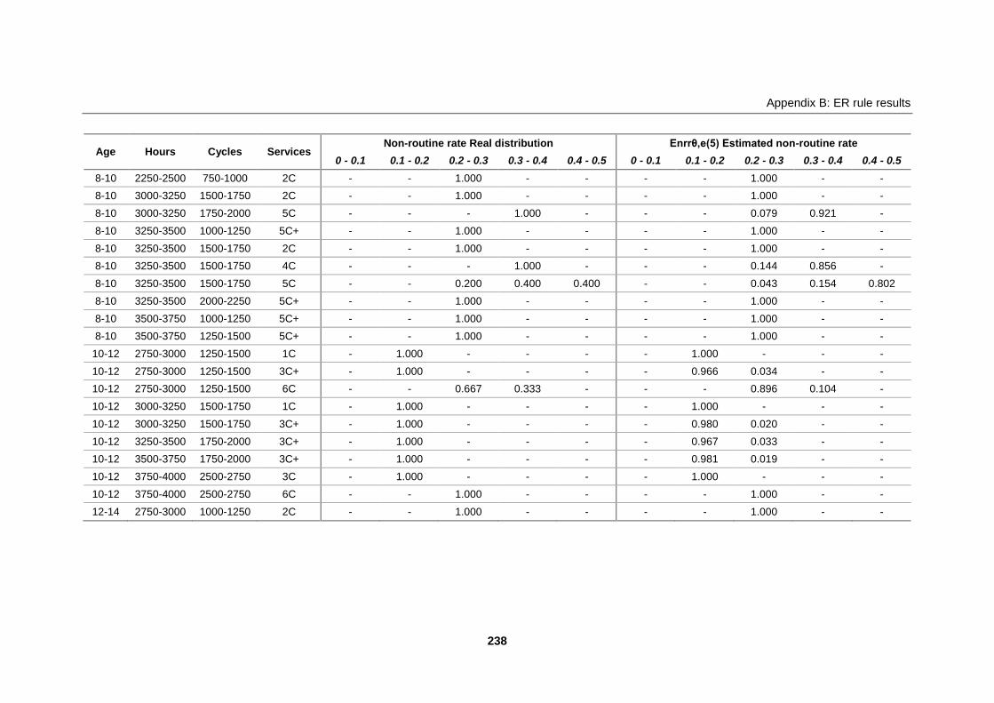
Appendix B: ER rule results
238
Age Hours Cycles Services Non-routine rate Real distribution Enrrθ,e(5) Estimated non-routine rate
0 - 0.1 0.1 - 0.2 0.2 - 0.3 0.3 - 0.4 0.4 - 0.5 0 - 0.1 0.1 - 0.2 0.2 - 0.3 0.3 - 0.4 0.4 - 0.5
8-10 2250-2500 750-1000 2C - - 1.000 - - - - 1.000 - -
8-10 3000-3250 1500-1750 2C - - 1.000 - - - - 1.000 - -
8-10 3000-3250 1750-2000 5C - - - 1.000 - - - 0.079 0.921 -
8-10 3250-3500 1000-1250 5C+ - - 1.000 - - - - 1.000 - -
8-10 3250-3500 1500-1750 2C - - 1.000 - - - - 1.000 - -
8-10 3250-3500 1500-1750 4C - - - 1.000 - - - 0.144 0.856 -
8-10 3250-3500 1500-1750 5C - - 0.200 0.400 0.400 - - 0.043 0.154 0.802
8-10 3250-3500 2000-2250 5C+ - - 1.000 - - - - 1.000 - -
8-10 3500-3750 1000-1250 5C+ - - 1.000 - - - - 1.000 - -
8-10 3500-3750 1250-1500 5C+ - - 1.000 - - - - 1.000 - -
10-12 2750-3000 1250-1500 1C - 1.000 - - - - 1.000 - - -
10-12 2750-3000 1250-1500 3C+ - 1.000 - - - - 0.966 0.034 - -
10-12 2750-3000 1250-1500 6C - - 0.667 0.333 - - - 0.896 0.104 -
10-12 3000-3250 1500-1750 1C - 1.000 - - - - 1.000 - - -
10-12 3000-3250 1500-1750 3C+ - 1.000 - - - - 0.980 0.020 - -
10-12 3250-3500 1750-2000 3C+ - 1.000 - - - - 0.967 0.033 - -
10-12 3500-3750 1750-2000 3C+ - 1.000 - - - - 0.981 0.019 - -
10-12 3750-4000 2500-2750 3C - 1.000 - - - - 1.000 - - -
10-12 3750-4000 2500-2750 6C - - 1.000 - - - - 1.000 - -
12-14 2750-3000 1000-1250 2C - - 1.000 - - - - 1.000 - -

Appendix B: ER rule results
239
Table B-7 Comparison between Real Non-routine rate and Estimated average Non-routine rate
Age (Years) Flight Hours / Year Cycles / Year Service
Type
Real Non-Routine
Rate
Estimated Average
Non-Routine Rate Value Interval Value Interval Value Interval
5.7 4-6 3,870.67 3750-4000 1,359 1250-1500 3C+ 0.128 0.150
5.7 4-6 3,946.89 3750-4000 1,479 1250-1500 3C 0.155 0.150
10.0 8-10 3,294.95 3250-3500 1,704 1500-1750 5C 0.374 0.426
6.2 6-8 3,733.39 3500-3750 1,599 1500-1750 2C 0.205 0.242
9.8 8-10 3,499.54 3250-3500 1,205 1000-1250 5C+ 0.270 0.250
7.8 6-8 3,365.26 3250-3500 1,797 1750-2000 4C+ 0.272 0.250
10.0 8-10 3,346.04 3250-3500 1,664 1500-1750 5C 0.468 0.426
10.0 8-10 3,323.99 3250-3500 1,693 1500-1750 5C 0.406 0.426
6.4 6-8 3,581.72 3500-3750 1,746 1500-1750 2C 0.140 0.242
6.4 6-8 3,761.30 3750-4000 1,615 1500-1750 2C 0.236 0.227
7.8 6-8 3,550.80 3500-3750 1,679 1500-1750 4C 0.296 0.317
7.9 6-8 3,290.86 3250-3500 1,763 1750-2000 4C 0.387 0.347
10.7 10-12 3,206.17 3000-3250 1,750 1500-1750 3C+ 0.157 0.152
7.5 6-8 3,309.39 3250-3500 1,793 1750-2000 1C 0.194 0.150
7.4 6-8 3,331.62 3250-3500 1,681 1500-1750 1C 0.160 0.150
9.4 8-10 3,395.93 3250-3500 1,682 1500-1750 2C 0.259 0.250
9.9 8-10 3,310.56 3250-3500 1,657 1500-1750 5C 0.392 0.426
5.5 4-6 3,607.77 3500-3750 1,753 1750-2000 3C+ 0.117 0.086
12.5 12-14 2,987.85 2750-3000 1,046 1000-1250 2C 0.269 0.250
9.4 8-10 3,410.21 3250-3500 1,672 1500-1750 2C 0.255 0.250
7.9 6-8 3,318.74 3250-3500 1,805 1750-2000 4C 0.357 0.347
5.6 4-6 3,873.21 3750-4000 1,498 1250-1500 3C 0.146 0.150
10.0 8-10 3,409.93 3250-3500 1,686 1500-1750 5C 0.244 0.426
7.9 6-8 3,508.23 3500-3750 1,814 1750-2000 4C+ 0.276 0.250
4.6 4-6 3,814.47 3750-4000 1,505 1500-1750 1C 0.106 0.150
9.1 8-10 3,334.74 3250-3500 2,044 2000-2250 5C+ 0.214 0.250
4.6 4-6 3,819.36 3750-4000 1,489 1250-1500 1C 0.121 0.150
7.2 6-8 3,290.43 3250-3500 1,759 1750-2000 1C 0.167 0.150
8.0 8-10 3,322.63 3250-3500 1,699 1500-1750 4C 0.334 0.336
9.9 8-10 3,241.95 3000-3250 1,905 1750-2000 5C 0.308 0.342

Appendix B: ER rule results
240
Age (Years) Flight Hours / Year Cycles / Year Service
Type
Real Non-Routine
Rate
Estimated Average
Non-Routine Rate Value Interval Value Interval Value Interval
7.3 6-8 3,285.89 3250-3500 1,581 1500-1750 1C 0.172 0.150
6.0 4-6 3,621.21 3500-3750 1,784 1750-2000 3C+ 0.153 0.086
5.4 4-6 4,467.20 4250-4500 1,919 1750-2000 3C 0.107 0.150
7.9 6-8 3,326.12 3250-3500 1,664 1500-1750 4C 0.359 0.344
9.3 8-10 3,363.37 3250-3500 1,702 1500-1750 2C 0.250 0.250
10.8 10-12 3,232.31 3000-3250 1,715 1500-1750 1C 0.167 0.150
11.5 10-12 2,906.01 2750-3000 1,471 1250-1500 1C 0.177 0.150
5.5 4-6 3,953.45 3750-4000 1,667 1500-1750 3C 0.129 0.150
6.4 6-8 3,612.33 3500-3750 1,730 1500-1750 2C 0.208 0.242
7.9 6-8 3,332.48 3250-3500 1,791 1750-2000 4C 0.378 0.347
5.8 4-6 3,906.89 3750-4000 1,498 1250-1500 3C 0.193 0.150
11.3 10-12 3,869.53 3750-4000 2,635 2500-2750 6C 0.235 0.250
7.5 6-8 3,565.79 3500-3750 1,687 1500-1750 2C 0.250 0.242
7.7 6-8 3,299.48 3250-3500 1,769 1750-2000 4C 0.389 0.347
9.7 8-10 3,502.16 3500-3750 1,202 1000-1250 5C+ 0.241 0.250
7.4 6-8 3,255.10 3250-3500 1,759 1750-2000 1C 0.187 0.150
9.6 8-10 3,694.48 3500-3750 1,282 1250-1500 5C+ 0.253 0.250
6.3 6-8 3,754.93 3750-4000 1,625 1500-1750 2C 0.114 0.227
5.7 4-6 3,916.89 3750-4000 1,398 1250-1500 3C+ 0.110 0.150
7.7 6-8 3,579.22 3500-3750 1,703 1500-1750 4C+ 0.274 0.250
8.0 6-8 3,336.73 3250-3500 1,669 1500-1750 4C 0.375 0.344
5.6 4-6 3,574.64 3500-3750 1,639 1500-1750 3C+ 0.122 0.150
11.9 10-12 2,929.50 2750-3000 1,473 1250-1500 6C 0.355 0.260
6.1 6-8 3,704.26 3500-3750 1,609 1500-1750 2C 0.234 0.242
5.4 4-6 3,543.50 3500-3750 1,722 1500-1750 3C 0.153 0.150
5.4 4-6 3,620.56 3500-3750 1,729 1500-1750 3C+ 0.112 0.150
7.6 6-8 3,376.86 3250-3500 1,678 1500-1750 1C 0.195 0.150
10.8 10-12 3,875.07 3750-4000 2,686 2500-2750 3C 0.132 0.150
7.8 6-8 3,565.96 3500-3750 1,681 1500-1750 4C 0.301 0.317
8.0 6-8 3,324.20 3250-3500 1,768 1750-2000 4C+ 0.221 0.250
10.4 10-12 3,628.94 3500-3750 1,909 1750-2000 3C+ 0.126 0.152
8.0 6-8 3,280.24 3250-3500 1,779 1750-2000 4C+ 0.273 0.250

Appendix B: ER rule results
241
Age (Years) Flight Hours / Year Cycles / Year Service
Type
Real Non-Routine
Rate
Estimated Average
Non-Routine Rate Value Interval Value Interval Value Interval
5.1 4-6 3,587.45 3500-3750 1,648 1500-1750 3C+ 0.116 0.150
5.2 4-6 3,636.00 3500-3750 1,808 1750-2000 3C+ 0.116 0.086
5.5 4-6 3,889.59 3750-4000 1,383 1250-1500 3C+ 0.105 0.150
6.0 4-6 3,961.20 3750-4000 1,476 1250-1500 2C 0.218 0.158
9.4 8-10 3,282.20 3250-3500 1,690 1500-1750 2C 0.262 0.250
9.3 8-10 3,332.37 3250-3500 1,680 1500-1750 2C 0.258 0.250
10.3 10-12 2,903.11 2750-3000 1,462 1250-1500 3C+ 0.109 0.153
9.4 8-10 3,345.00 3250-3500 2,043 2000-2250 5C+ 0.270 0.250
9.4 8-10 2,416.95 2250-2500 959 750-1000 2C 0.205 0.250
7.8 6-8 3,380.84 3250-3500 1,678 1500-1750 4C 0.253 0.344
6.1 6-8 3,746.23 3500-3750 1,540 1500-1750 1C 0.132 0.150
11.9 10-12 2,945.41 2750-3000 1,379 1250-1500 6C 0.211 0.260
7.6 6-8 3,559.61 3500-3750 1,684 1500-1750 3C+ 0.236 0.159
7.4 6-8 3,290.91 3250-3500 1,753 1750-2000 1C 0.160 0.150
9.4 8-10 3,357.15 3250-3500 1,690 1500-1750 2C 0.293 0.250
7.9 6-8 3,350.86 3250-3500 1,805 1750-2000 4C+ 0.275 0.250
7.8 6-8 3,346.15 3250-3500 1,712 1500-1750 4C 0.362 0.344
5.3 4-6 3,599.66 3500-3750 1,773 1750-2000 3C+ 0.096 0.086
5.7 4-6 4,024.75 4000-4250 1,527 1500-1750 3C+ 0.149 0.150
9.6 8-10 3,702.64 3500-3750 1,273 1250-1500 5C+ 0.201 0.250
11.8 10-12 2,954.58 2750-3000 1,381 1250-1500 6C 0.232 0.260
10.6 10-12 3,251.48 3250-3500 1,900 1750-2000 3C+ 0.177 0.153
7.7 6-8 3,321.49 3250-3500 1,746 1500-1750 4C 0.337 0.344
5.9 4-6 3,551.08 3500-3750 1,744 1500-1750 3C 0.120 0.150
5.3 4-6 3,666.47 3500-3750 1,606 1500-1750 3C 0.143 0.150
7.5 6-8 3,306.48 3250-3500 1,653 1500-1750 1C 0.151 0.150
9.3 8-10 3,205.10 3000-3250 1,690 1500-1750 2C 0.242 0.250
7.6 6-8 3,346.97 3250-3500 1,709 1500-1750 1C 0.162 0.150
9.1 8-10 3,295.27 3250-3500 1,600 1500-1750 2C 0.208 0.250

Appendix B: ER rule results
242
B.4 Bin size and interval limits analysis
Table B-8 Model performance comparison for different bin-widths of flight and cycles per year;
considering interval-widths of 0.05 for non-routine rate and 0.5 for aircraft’s age, with 4.5 and 13.0
years as lower and upper limits.
Bin-width Model Performance Indicators
Fh / Y Cy / Y MSEDIST MSESERV MAE MAPE MAI
100 100 0.0211 0.0008 0.0196 10.1% 95.4%
100 150 0.0241 0.0009 0.0206 10.6% 95.1%
100 200 0.0281 0.0009 0.0207 10.7% 95.1%
100 250 0.0257 0.0009 0.0209 10.7% 95.1%
100 300 0.0264 0.0009 0.0209 10.7% 95.1%
150 100 0.0175 0.0007 0.0188 10.0% 95.6%
150 150 0.0193 0.0008 0.0199 10.3% 95.3%
150 200 0.0206 0.0008 0.0198 10.3% 95.3%
150 250 0.0218 0.0008 0.0204 10.6% 95.2%
150 300 0.0177 0.0008 0.0198 10.2% 95.3%
200 100 0.0207 0.0009 0.0202 10.4% 95.3%
200 150 0.0244 0.0010 0.0217 10.9% 94.9%
200 200 0.0285 0.0010 0.0216 11.0% 94.9%
200 250 0.0253 0.0010 0.0217 10.9% 94.9%
200 300 0.0261 0.0010 0.0216 10.9% 94.9%
250 100 0.0176 0.0012 0.0219 11.2% 94.9%
250 150 0.0191 0.0013 0.0227 11.4% 94.6%
250 200 0.0179 0.0013 0.0228 11.4% 94.6%
250 250 0.0166 0.0013 0.0230 11.5% 94.6%
250 300 0.0147 0.0013 0.0228 11.3% 94.6%
300 100 0.0184 0.0012 0.0219 11.2% 94.8%
300 150 0.0209 0.0013 0.0231 11.5% 94.6%
300 200 0.0199 0.0013 0.0231 11.5% 94.6%
300 250 0.0199 0.0014 0.0234 11.7% 94.5%
300 300 0.0170 0.0013 0.0231 11.4% 94.6%

Appendix B: ER rule results
243
Table B-9 Model performance comparison for different bin-widths of flight and cycles per year;
considering interval-widths of 0.05 for non-routine rate and 1.0 for aircraft’s age, with 4.0 and 13.0
years as lower and upper limits.
Bin-width Model Performance Indicators
Fh / Y Cy / Y MSEDIST MSESERV MAE MAPE MAI
100 100 0.0193 0.0008 0.0199 10.3% 95.3%
100 150 0.0211 0.0009 0.0206 10.6% 95.1%
100 200 0.0252 0.0009 0.0210 10.8% 95.1%
100 250 0.0236 0.0009 0.0211 10.7% 95.0%
100 300 0.0230 0.0009 0.0209 10.8% 95.1%
150 100 0.0153 0.0008 0.0194 10.3% 95.4%
150 150 0.0157 0.0008 0.0200 10.3% 95.3%
150 200 0.0193 0.0008 0.0200 10.4% 95.3%
150 250 0.0192 0.0009 0.0208 10.8% 95.1%
150 300 0.0158 0.0008 0.0199 10.3% 95.3%
200 100 0.0181 0.0009 0.0202 10.5% 95.2%
200 150 0.0203 0.0010 0.0214 10.8% 95.0%
200 200 0.0246 0.0010 0.0216 11.0% 94.9%
200 250 0.0221 0.0010 0.0214 10.8% 95.0%
200 300 0.0215 0.0010 0.0214 10.8% 95.0%
250 100 0.0148 0.0013 0.0222 11.3% 94.8%
250 150 0.0145 0.0013 0.0228 11.4% 94.6%
250 200 0.0187 0.0013 0.0228 11.4% 94.6%
250 250 0.0159 0.0014 0.0230 11.6% 94.6%
250 300 0.0152 0.0013 0.0226 11.3% 94.7%
300 100 0.0152 0.0013 0.0221 11.3% 94.8%
300 150 0.0161 0.0014 0.0231 11.5% 94.6%
300 200 0.0208 0.0014 0.0230 11.5% 94.6%
300 250 0.0193 0.0014 0.0234 11.7% 94.5%
300 300 0.0176 0.0014 0.0228 11.3% 94.6%
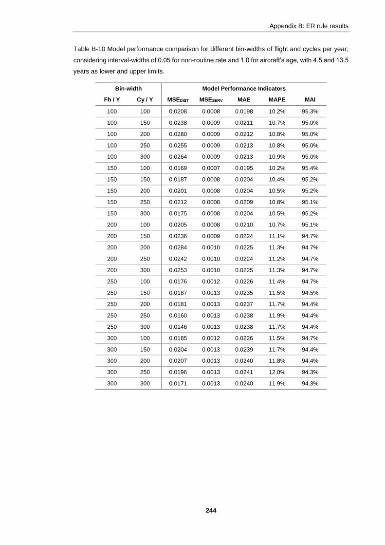
Appendix B: ER rule results
244
Table B-10 Model performance comparison for different bin-widths of flight and cycles per year;
considering interval-widths of 0.05 for non-routine rate and 1.0 for aircraft’s age, with 4.5 and 13.5
years as lower and upper limits.
Bin-width Model Performance Indicators
Fh / Y Cy / Y MSEDIST MSESERV MAE MAPE MAI
100 100 0.0208 0.0008 0.0198 10.2% 95.3%
100 150 0.0238 0.0009 0.0211 10.7% 95.0%
100 200 0.0280 0.0009 0.0212 10.8% 95.0%
100 250 0.0255 0.0009 0.0213 10.8% 95.0%
100 300 0.0264 0.0009 0.0213 10.9% 95.0%
150 100 0.0169 0.0007 0.0195 10.2% 95.4%
150 150 0.0187 0.0008 0.0204 10.4% 95.2%
150 200 0.0201 0.0008 0.0204 10.5% 95.2%
150 250 0.0212 0.0008 0.0209 10.8% 95.1%
150 300 0.0175 0.0008 0.0204 10.5% 95.2%
200 100 0.0205 0.0008 0.0210 10.7% 95.1%
200 150 0.0236 0.0009 0.0224 11.1% 94.7%
200 200 0.0284 0.0010 0.0225 11.3% 94.7%
200 250 0.0242 0.0010 0.0224 11.2% 94.7%
200 300 0.0253 0.0010 0.0225 11.3% 94.7%
250 100 0.0176 0.0012 0.0226 11.4% 94.7%
250 150 0.0187 0.0013 0.0235 11.5% 94.5%
250 200 0.0181 0.0013 0.0237 11.7% 94.4%
250 250 0.0160 0.0013 0.0238 11.9% 94.4%
250 300 0.0146 0.0013 0.0238 11.7% 94.4%
300 100 0.0185 0.0012 0.0226 11.5% 94.7%
300 150 0.0204 0.0013 0.0239 11.7% 94.4%
300 200 0.0207 0.0013 0.0240 11.8% 94.4%
300 250 0.0196 0.0013 0.0241 12.0% 94.3%
300 300 0.0171 0.0013 0.0240 11.9% 94.3%

Appendix B: ER rule results
245
Table B-11 Model performance comparison for different bin-widths of flight and cycles per year;
considering interval-widths of 0.05 for non-routine rate and 1.5 for aircraft’s age, with 4.0 and 13.0
years as lower and upper limits.
Bin-width Model Performance Indicators
Fh / Y Cy / Y MSEDIST MSESERV MAE MAPE MAI
100 100 0.0224 0.0008 0.0199 10.3% 95.3%
100 150 0.0270 0.0009 0.0213 10.8% 95.0%
100 200 0.0288 0.0009 0.0212 10.8% 95.0%
100 250 0.0289 0.0009 0.0215 10.9% 94.9%
100 300 0.0295 0.0009 0.0214 10.9% 95.0%
150 100 0.0193 0.0007 0.0197 10.4% 95.4%
150 150 0.0229 0.0008 0.0207 10.5% 95.1%
150 200 0.0217 0.0008 0.0204 10.5% 95.2%
150 250 0.0263 0.0008 0.0212 10.9% 95.0%
150 300 0.0215 0.0008 0.0204 10.4% 95.2%
200 100 0.0220 0.0008 0.0208 10.7% 95.1%
200 150 0.0270 0.0009 0.0225 11.1% 94.7%
200 200 0.0292 0.0009 0.0222 11.2% 94.8%
200 250 0.0281 0.0009 0.0223 11.1% 94.8%
200 300 0.0288 0.0009 0.0222 11.1% 94.8%
250 100 0.0200 0.0012 0.0226 11.5% 94.7%
250 150 0.0230 0.0013 0.0237 11.6% 94.4%
250 200 0.0196 0.0013 0.0234 11.6% 94.5%
250 250 0.0214 0.0013 0.0238 11.9% 94.4%
250 300 0.0190 0.0013 0.0235 11.6% 94.5%
300 100 0.0208 0.0012 0.0226 11.5% 94.7%
300 150 0.0248 0.0013 0.0240 11.8% 94.3%
300 200 0.0222 0.0013 0.0236 11.7% 94.4%
300 250 0.0252 0.0013 0.0241 12.0% 94.3%
300 300 0.0217 0.0013 0.0237 11.7% 94.4%

Appendix B: ER rule results
246
Table B-12 Model performance comparison for different bin-widths of flight and cycles per year;
considering interval-widths of 0.05 for non-routine rate and 1.5 for aircraft’s age, with 4.5 and 13.5
years as lower and upper limits.
Bin-width Model Performance Indicators
Fh / Y Cy / Y MSEDIST MSESERV MAE MAPE MAI
100 100 0.0198 0.0009 0.0202 10.6% 95.2%
100 150 0.0204 0.0010 0.0215 11.1% 95.0%
100 200 0.0239 0.0010 0.0215 11.1% 94.9%
100 250 0.0226 0.0010 0.0218 11.2% 94.9%
100 300 0.0226 0.0010 0.0219 11.4% 94.8%
150 100 0.0165 0.0008 0.0203 10.8% 95.2%
150 150 0.0165 0.0009 0.0214 11.2% 95.0%
150 200 0.0196 0.0009 0.0212 11.2% 95.0%
150 250 0.0197 0.0010 0.0221 11.7% 94.8%
150 300 0.0178 0.0009 0.0215 11.4% 94.9%
200 100 0.0191 0.0009 0.0210 11.1% 95.1%
200 150 0.0187 0.0011 0.0225 11.5% 94.7%
200 200 0.0240 0.0011 0.0227 11.8% 94.7%
200 250 0.0221 0.0011 0.0228 11.8% 94.6%
200 300 0.0234 0.0011 0.0231 12.1% 94.6%
250 100 0.0152 0.0013 0.0230 11.9% 94.6%
250 150 0.0152 0.0014 0.0240 12.1% 94.4%
250 200 0.0208 0.0014 0.0240 12.2% 94.4%
250 250 0.0184 0.0014 0.0245 12.6% 94.2%
250 300 0.0198 0.0014 0.0244 12.5% 94.3%
300 100 0.0152 0.0013 0.0230 11.9% 94.6%
300 150 0.0167 0.0014 0.0243 12.2% 94.3%
300 200 0.0228 0.0014 0.0242 12.3% 94.3%
300 250 0.0216 0.0015 0.0248 12.8% 94.2%
300 300 0.0222 0.0015 0.0246 12.7% 94.2%

Appendix B: ER rule results
247
Table B-13 Model performance comparison for different bin-widths of flight and cycles per year;
considering interval-widths of 0.05 for non-routine rate and 2.0 for aircraft’s age, with 3.0 and 13.0
years as lower and upper limits.
Bin-width Model Performance Indicators
Fh / Y Cy / Y MSEDIST MSESERV MAE MAPE MAI
100 100 0.0192 0.0008 0.0202 10.4% 95.2%
100 150 0.0237 0.0009 0.0216 10.9% 94.9%
100 200 0.0253 0.0009 0.0216 11.0% 94.9%
100 250 0.0257 0.0009 0.0218 11.0% 94.9%
100 300 0.0261 0.0009 0.0219 11.1% 94.8%
150 100 0.0148 0.0007 0.0200 10.4% 95.3%
150 150 0.0182 0.0008 0.0211 10.6% 95.0%
150 200 0.0193 0.0008 0.0208 10.6% 95.1%
150 250 0.0213 0.0009 0.0217 11.0% 94.9%
150 300 0.0191 0.0008 0.0209 10.6% 95.1%
200 100 0.0181 0.0008 0.0211 10.7% 95.0%
200 150 0.0230 0.0010 0.0228 11.2% 94.6%
200 200 0.0247 0.0010 0.0225 11.2% 94.7%
200 250 0.0236 0.0010 0.0227 11.3% 94.7%
200 300 0.0241 0.0010 0.0229 11.4% 94.6%
250 100 0.0154 0.0013 0.0231 11.5% 94.6%
250 150 0.0184 0.0014 0.0242 11.8% 94.3%
250 200 0.0201 0.0013 0.0238 11.6% 94.4%
250 250 0.0191 0.0014 0.0244 12.1% 94.3%
250 300 0.0199 0.0014 0.0241 11.8% 94.3%
300 100 0.0157 0.0013 0.0230 11.5% 94.6%
300 150 0.0197 0.0014 0.0245 11.9% 94.2%
300 200 0.0228 0.0013 0.0240 11.7% 94.4%
300 250 0.0229 0.0014 0.0247 12.2% 94.2%
300 300 0.0228 0.0014 0.0243 11.9% 94.3%

Appendix B: ER rule results
248
Table B-14 Model performance comparison for different bin-widths of flight and cycles per year;
considering interval-widths of 0.05 for non-routine rate and 2.0 for aircraft’s age, with 4.0 and 14.0
years as lower and upper limits.
Bin-width Model Performance Indicators
Fh / Y Cy / Y MSEDIST MSESERV MAE MAPE MAI
100 100 0.0227 0.0010 0.0210 11.1% 95.1%
100 150 0.0218 0.0011 0.0218 11.4% 94.9%
100 200 0.0254 0.0011 0.0220 11.5% 94.8%
100 250 0.0239 0.0011 0.0221 11.5% 94.8%
100 300 0.0235 0.0011 0.0221 11.6% 94.8%
150 100 0.0187 0.0010 0.0210 11.4% 95.1%
150 150 0.0164 0.0010 0.0215 11.3% 94.9%
150 200 0.0200 0.0010 0.0214 11.5% 95.0%
150 250 0.0204 0.0011 0.0223 11.9% 94.8%
150 300 0.0176 0.0011 0.0215 11.5% 94.9%
200 100 0.0232 0.0011 0.0217 11.6% 94.9%
200 150 0.0202 0.0012 0.0226 11.7% 94.7%
200 200 0.0261 0.0012 0.0227 12.0% 94.6%
200 250 0.0243 0.0012 0.0231 12.1% 94.6%
200 300 0.0249 0.0012 0.0232 12.3% 94.5%
250 100 0.0201 0.0015 0.0238 12.4% 94.4%
250 150 0.0168 0.0015 0.0241 12.3% 94.3%
250 200 0.0240 0.0015 0.0242 12.5% 94.3%
250 250 0.0224 0.0015 0.0251 13.0% 94.1%
250 300 0.0227 0.0015 0.0248 12.8% 94.2%
300 100 0.0202 0.0015 0.0239 12.6% 94.4%
300 150 0.0173 0.0015 0.0242 12.3% 94.3%
300 200 0.0250 0.0016 0.0244 12.7% 94.3%
300 250 0.0244 0.0016 0.0254 13.2% 94.0%
300 300 0.0240 0.0016 0.0249 13.0% 94.1%

Appendix B: ER rule results
249
Table B-15 Model performance comparison for different bin-widths of flight and cycles per year;
considering interval-widths of 0.05 for non-routine rate and 2.5 for aircraft’s age, with 2.5 and 15.0
years as lower and upper limits.
Bin-width Model Performance Indicators
Fh / Y Cy / Y MSEDIST MSESERV MAE MAPE MAI
100 100 0.0175 0.0008 0.0200 10.4% 95.3%
100 150 0.0172 0.0009 0.0211 10.8% 95.0%
100 200 0.0211 0.0009 0.0214 11.0% 95.0%
100 250 0.0192 0.0009 0.0214 10.9% 95.0%
100 300 0.0183 0.0009 0.0215 11.0% 94.9%
150 100 0.0136 0.0007 0.0197 10.3% 95.4%
150 150 0.0117 0.0008 0.0203 10.4% 95.2%
150 200 0.0157 0.0008 0.0203 10.4% 95.2%
150 250 0.0145 0.0008 0.0210 10.8% 95.1%
150 300 0.0114 0.0008 0.0201 10.3% 95.3%
200 100 0.0181 0.0009 0.0211 10.8% 95.0%
200 150 0.0159 0.0010 0.0223 11.2% 94.8%
200 200 0.0215 0.0010 0.0225 11.4% 94.7%
200 250 0.0174 0.0010 0.0224 11.3% 94.7%
200 300 0.0169 0.0010 0.0225 11.4% 94.7%
250 100 0.0125 0.0012 0.0225 11.3% 94.7%
250 150 0.0109 0.0012 0.0231 11.4% 94.6%
250 200 0.0162 0.0012 0.0231 11.4% 94.6%
250 250 0.0119 0.0012 0.0235 11.7% 94.5%
250 300 0.0112 0.0012 0.0230 11.3% 94.6%
300 100 0.0128 0.0012 0.0224 11.4% 94.7%
300 150 0.0120 0.0012 0.0234 11.5% 94.5%
300 200 0.0188 0.0012 0.0233 11.5% 94.5%
300 250 0.0157 0.0013 0.0238 11.9% 94.4%
300 300 0.0138 0.0012 0.0233 11.5% 94.5%
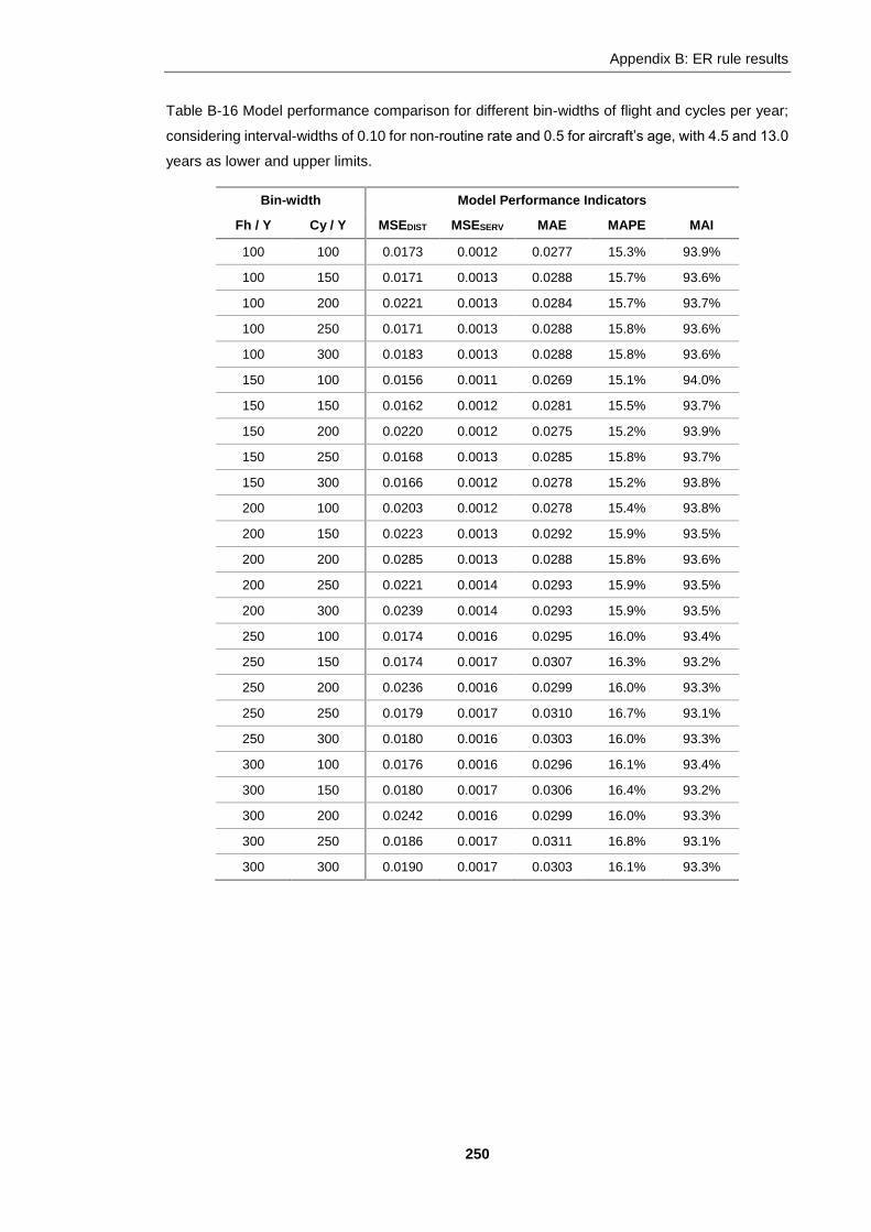
Appendix B: ER rule results
250
Table B-16 Model performance comparison for different bin-widths of flight and cycles per year;
considering interval-widths of 0.10 for non-routine rate and 0.5 for aircraft’s age, with 4.5 and 13.0
years as lower and upper limits.
Bin-width Model Performance Indicators
Fh / Y Cy / Y MSEDIST MSESERV MAE MAPE MAI
100 100 0.0173 0.0012 0.0277 15.3% 93.9%
100 150 0.0171 0.0013 0.0288 15.7% 93.6%
100 200 0.0221 0.0013 0.0284 15.7% 93.7%
100 250 0.0171 0.0013 0.0288 15.8% 93.6%
100 300 0.0183 0.0013 0.0288 15.8% 93.6%
150 100 0.0156 0.0011 0.0269 15.1% 94.0%
150 150 0.0162 0.0012 0.0281 15.5% 93.7%
150 200 0.0220 0.0012 0.0275 15.2% 93.9%
150 250 0.0168 0.0013 0.0285 15.8% 93.7%
150 300 0.0166 0.0012 0.0278 15.2% 93.8%
200 100 0.0203 0.0012 0.0278 15.4% 93.8%
200 150 0.0223 0.0013 0.0292 15.9% 93.5%
200 200 0.0285 0.0013 0.0288 15.8% 93.6%
200 250 0.0221 0.0014 0.0293 15.9% 93.5%
200 300 0.0239 0.0014 0.0293 15.9% 93.5%
250 100 0.0174 0.0016 0.0295 16.0% 93.4%
250 150 0.0174 0.0017 0.0307 16.3% 93.2%
250 200 0.0236 0.0016 0.0299 16.0% 93.3%
250 250 0.0179 0.0017 0.0310 16.7% 93.1%
250 300 0.0180 0.0016 0.0303 16.0% 93.3%
300 100 0.0176 0.0016 0.0296 16.1% 93.4%
300 150 0.0180 0.0017 0.0306 16.4% 93.2%
300 200 0.0242 0.0016 0.0299 16.0% 93.3%
300 250 0.0186 0.0017 0.0311 16.8% 93.1%
300 300 0.0190 0.0017 0.0303 16.1% 93.3%

Appendix B: ER rule results
251
Table B-17 Model performance comparison for different bin-widths of flight and cycles per year;
considering interval-widths of 0.10 for non-routine rate and 1.0 for aircraft’s age, with 4.0 and 13.0
years as lower and upper limits.
Bin-width Model Performance Indicators
Fh / Y Cy / Y MSEDIST MSESERV MAE MAPE MAI
100 100 0.0211 0.0012 0.0277 15.2% 93.8%
100 150 0.0203 0.0013 0.0284 15.5% 93.7%
100 200 0.0257 0.0013 0.0281 15.4% 93.7%
100 250 0.0203 0.0013 0.0285 15.6% 93.7%
100 300 0.0214 0.0013 0.0283 15.4% 93.7%
150 100 0.0183 0.0012 0.0271 15.0% 94.0%
150 150 0.0175 0.0012 0.0277 15.1% 93.8%
150 200 0.0236 0.0012 0.0269 14.6% 94.0%
150 250 0.0189 0.0013 0.0284 15.7% 93.7%
150 300 0.0175 0.0012 0.0269 14.6% 94.0%
200 100 0.0238 0.0012 0.0277 15.2% 93.9%
200 150 0.0244 0.0013 0.0285 15.5% 93.7%
200 200 0.0315 0.0013 0.0281 15.4% 93.8%
200 250 0.0250 0.0013 0.0286 15.6% 93.6%
200 300 0.0263 0.0013 0.0283 15.4% 93.7%
250 100 0.0209 0.0016 0.0296 15.9% 93.4%
250 150 0.0192 0.0016 0.0301 15.9% 93.3%
250 200 0.0260 0.0016 0.0291 15.4% 93.5%
250 250 0.0205 0.0017 0.0307 16.5% 93.2%
250 300 0.0197 0.0016 0.0293 15.4% 93.5%
300 100 0.0212 0.0016 0.0296 15.9% 93.4%
300 150 0.0199 0.0017 0.0300 15.9% 93.3%
300 200 0.0267 0.0016 0.0291 15.4% 93.5%
300 250 0.0213 0.0017 0.0307 16.5% 93.2%
300 300 0.0209 0.0016 0.0292 15.4% 93.5%

Appendix B: ER rule results
252
Table B-18 Model performance comparison for different bin-widths of flight and cycles per year;
considering interval-widths of 0.10 for non-routine rate and 1.0 for aircraft’s age, with 4.5 and 13.5
years as lower and upper limits.
Bin-width Model Performance Indicators
Fh / Y Cy / Y MSEDIST MSESERV MAE MAPE MAI
100 100 0.0166 0.0011 0.0271 15.0% 94.0%
100 150 0.0152 0.0012 0.0279 15.3% 93.8%
100 200 0.0212 0.0012 0.0274 15.2% 93.9%
100 250 0.0148 0.0013 0.0280 15.4% 93.8%
100 300 0.0157 0.0013 0.0280 15.4% 93.8%
150 100 0.0138 0.0010 0.0257 14.4% 94.3%
150 150 0.0127 0.0011 0.0272 14.9% 94.0%
150 200 0.0198 0.0011 0.0263 14.5% 94.2%
150 250 0.0132 0.0012 0.0275 15.3% 93.9%
150 300 0.0132 0.0011 0.0267 14.6% 94.1%
200 100 0.0201 0.0011 0.0270 15.0% 94.0%
200 150 0.0204 0.0013 0.0289 15.6% 93.6%
200 200 0.0284 0.0012 0.0284 15.6% 93.7%
200 250 0.0189 0.0013 0.0287 15.7% 93.6%
200 300 0.0204 0.0013 0.0287 15.7% 93.6%
250 100 0.0159 0.0015 0.0285 15.4% 93.7%
250 150 0.0153 0.0016 0.0301 15.9% 93.3%
250 200 0.0230 0.0015 0.0293 15.5% 93.5%
250 250 0.0143 0.0016 0.0304 16.3% 93.2%
250 300 0.0145 0.0015 0.0296 15.6% 93.4%
300 100 0.0169 0.0015 0.0284 15.4% 93.7%
300 150 0.0155 0.0016 0.0300 16.0% 93.3%
300 200 0.0247 0.0015 0.0292 15.5% 93.5%
300 250 0.0158 0.0016 0.0304 16.4% 93.3%
300 300 0.0161 0.0016 0.0295 15.6% 93.4%

Appendix B: ER rule results
253
Table B-19 Model performance comparison for different bin-widths of flight and cycles per year;
considering interval-widths of 0.10 for non-routine rate and 1.5 for aircraft’s age, with 4.0 and 13.0
years as lower and upper limits.
Bin-width Model Performance Indicators
Fh / Y Cy / Y MSEDIST MSESERV MAE MAPE MAI
100 100 0.0190 0.0012 0.0272 15.0% 94.0%
100 150 0.0165 0.0012 0.0275 15.1% 93.9%
100 200 0.0233 0.0012 0.0272 15.0% 93.9%
100 250 0.0160 0.0012 0.0276 15.2% 93.9%
100 300 0.0167 0.0012 0.0274 15.1% 93.9%
150 100 0.0157 0.0010 0.0256 14.3% 94.3%
150 150 0.0128 0.0011 0.0265 14.5% 94.1%
150 200 0.0208 0.0011 0.0258 14.2% 94.3%
150 250 0.0134 0.0012 0.0268 14.9% 94.1%
150 300 0.0126 0.0011 0.0258 14.1% 94.3%
200 100 0.0220 0.0011 0.0269 14.9% 94.0%
200 150 0.0202 0.0012 0.0281 15.2% 93.8%
200 200 0.0293 0.0012 0.0278 15.3% 93.8%
200 250 0.0192 0.0012 0.0279 15.2% 93.8%
200 300 0.0198 0.0012 0.0277 15.1% 93.8%
250 100 0.0187 0.0015 0.0284 15.3% 93.7%
250 150 0.0161 0.0015 0.0294 15.5% 93.5%
250 200 0.0248 0.0015 0.0288 15.2% 93.6%
250 250 0.0151 0.0015 0.0296 15.8% 93.4%
250 300 0.0145 0.0015 0.0285 15.0% 93.7%
300 100 0.0198 0.0015 0.0284 15.4% 93.7%
300 150 0.0163 0.0015 0.0293 15.6% 93.5%
300 200 0.0267 0.0015 0.0286 15.2% 93.7%
300 250 0.0168 0.0016 0.0295 15.9% 93.4%
300 300 0.0163 0.0015 0.0284 15.1% 93.7%

Appendix B: ER rule results
254
Table B-20 Model performance comparison for different bin-widths of flight and cycles per year;
considering interval-widths of 0.10 for non-routine rate and 1.5 for aircraft’s age, with 4.5 and 13.5
years as lower and upper limits.
Bin-width Model Performance Indicators
Fh / Y Cy / Y MSEDIST MSESERV MAE MAPE MAI
100 100 0.0195 0.0012 0.0273 15.1% 93.9%
100 150 0.0150 0.0013 0.0281 15.5% 93.8%
100 200 0.0205 0.0013 0.0277 15.3% 93.8%
100 250 0.0156 0.0013 0.0285 15.8% 93.7%
100 300 0.0174 0.0013 0.0283 15.6% 93.7%
150 100 0.0167 0.0011 0.0264 14.7% 94.1%
150 150 0.0162 0.0012 0.0275 15.1% 93.9%
150 200 0.0226 0.0012 0.0266 14.6% 94.1%
150 250 0.0179 0.0013 0.0284 15.9% 93.7%
150 300 0.0183 0.0012 0.0272 14.9% 94.0%
200 100 0.0217 0.0012 0.0270 14.9% 94.0%
200 150 0.0181 0.0013 0.0286 15.6% 93.6%
200 200 0.0256 0.0013 0.0279 15.3% 93.8%
200 250 0.0183 0.0013 0.0286 15.8% 93.6%
200 300 0.0213 0.0013 0.0286 15.8% 93.7%
250 100 0.0186 0.0015 0.0289 15.5% 93.6%
250 150 0.0182 0.0016 0.0303 16.0% 93.3%
250 200 0.0259 0.0015 0.0290 15.3% 93.6%
250 250 0.0199 0.0017 0.0309 16.7% 93.1%
250 300 0.0216 0.0016 0.0297 15.7% 93.4%
300 100 0.0189 0.0016 0.0289 15.5% 93.6%
300 150 0.0185 0.0016 0.0301 16.1% 93.3%
300 200 0.0272 0.0016 0.0287 15.3% 93.6%
300 250 0.0211 0.0017 0.0307 16.7% 93.2%
300 300 0.0233 0.0017 0.0294 15.8% 93.5%

Appendix B: ER rule results
255
Table B-21 Model performance comparison for different bin-widths of flight and cycles per year;
considering interval-widths of 0.10 for non-routine rate and 2.0 for aircraft’s age, with 3.0 and 13.0
years as lower and upper limits.
Bin-width Model Performance Indicators
Fh / Y Cy / Y MSEDIST MSESERV MAE MAPE MAI
100 100 0.0217 0.0012 0.0270 14.8% 94.0%
100 150 0.0189 0.0012 0.0275 15.0% 93.9%
100 200 0.0263 0.0012 0.0270 14.7% 94.0%
100 250 0.0183 0.0012 0.0276 15.2% 93.9%
100 300 0.0191 0.0012 0.0272 14.8% 94.0%
150 100 0.0179 0.0011 0.0257 14.2% 94.3%
150 150 0.0143 0.0011 0.0265 14.3% 94.1%
150 200 0.0231 0.0011 0.0256 13.8% 94.3%
150 250 0.0149 0.0012 0.0270 15.0% 94.0%
150 300 0.0140 0.0011 0.0255 13.8% 94.3%
200 100 0.0254 0.0011 0.0273 15.0% 93.9%
200 150 0.0237 0.0012 0.0282 15.2% 93.7%
200 200 0.0335 0.0012 0.0279 15.1% 93.8%
200 250 0.0222 0.0012 0.0281 15.3% 93.8%
200 300 0.0232 0.0012 0.0276 15.0% 93.9%
250 100 0.0213 0.0015 0.0287 15.2% 93.6%
250 150 0.0188 0.0015 0.0293 15.3% 93.5%
250 200 0.0283 0.0015 0.0285 14.8% 93.7%
250 250 0.0177 0.0016 0.0298 15.8% 93.4%
250 300 0.0178 0.0015 0.0283 14.7% 93.7%
300 100 0.0224 0.0015 0.0287 15.3% 93.6%
300 150 0.0188 0.0015 0.0295 15.5% 93.5%
300 200 0.0305 0.0015 0.0285 15.0% 93.7%
300 250 0.0198 0.0016 0.0299 16.0% 93.4%
300 300 0.0199 0.0015 0.0284 14.9% 93.7%

Appendix B: ER rule results
256
Table B-22 Model performance comparison for different bin-widths of flight and cycles per year;
considering interval-widths of 0.10 for non-routine rate and 2.0 for aircraft’s age, with 4.0 and 14.0
years as lower and upper limits.
Bin-width Model Performance Indicators
Fh / Y Cy / Y MSEDIST MSESERV MAE MAPE MAI
100 100 0.0209 0.0012 0.0273 15.1% 93.9%
100 150 0.0155 0.0013 0.0281 15.4% 93.7%
100 200 0.0208 0.0013 0.0278 15.2% 93.8%
100 250 0.0155 0.0013 0.0282 15.5% 93.7%
100 300 0.0163 0.0013 0.0280 15.3% 93.8%
150 100 0.0178 0.0011 0.0266 14.8% 94.1%
150 150 0.0163 0.0012 0.0273 14.9% 93.9%
150 200 0.0225 0.0012 0.0265 14.4% 94.1%
150 250 0.0177 0.0013 0.0280 15.5% 93.8%
150 300 0.0164 0.0012 0.0266 14.4% 94.1%
200 100 0.0238 0.0012 0.0273 15.1% 93.9%
200 150 0.0191 0.0013 0.0282 15.4% 93.7%
200 200 0.0260 0.0013 0.0277 15.2% 93.8%
200 250 0.0193 0.0013 0.0283 15.5% 93.7%
200 300 0.0203 0.0013 0.0280 15.3% 93.8%
250 100 0.0209 0.0016 0.0290 15.6% 93.6%
250 150 0.0180 0.0016 0.0297 15.7% 93.4%
250 200 0.0256 0.0015 0.0286 15.1% 93.6%
250 250 0.0202 0.0017 0.0302 16.3% 93.3%
250 300 0.0194 0.0016 0.0289 15.2% 93.6%
300 100 0.0209 0.0016 0.0290 15.6% 93.5%
300 150 0.0186 0.0016 0.0295 15.7% 93.4%
300 200 0.0264 0.0016 0.0285 15.1% 93.7%
300 250 0.0210 0.0017 0.0302 16.3% 93.3%
300 300 0.0205 0.0016 0.0287 15.2% 93.6%

Appendix B: ER rule results
257
Table B-23 Model performance comparison for different bin-widths of flight and cycles per year;
considering interval-widths of 0.10 for non-routine rate and 2.5 for aircraft’s age, with 2.5 and 15.0
years as lower and upper limits.
Bin-width Model Performance Indicators
Fh / Y Cy / Y MSEDIST MSESERV MAE MAPE MAI
100 100 0.0170 0.0011 0.0260 14.4% 94.2%
100 150 0.0109 0.0011 0.0268 14.6% 94.0%
100 200 0.0174 0.0011 0.0261 14.3% 94.2%
100 250 0.0098 0.0011 0.0268 14.7% 94.0%
100 300 0.0100 0.0011 0.0264 14.3% 94.1%
150 100 0.0128 0.0010 0.0247 13.7% 94.5%
150 150 0.0085 0.0010 0.0256 13.9% 94.3%
150 200 0.0170 0.0010 0.0245 13.3% 94.6%
150 250 0.0083 0.0011 0.0258 14.3% 94.3%
150 300 0.0076 0.0010 0.0245 13.2% 94.5%
200 100 0.0211 0.0011 0.0263 14.6% 94.1%
200 150 0.0149 0.0012 0.0274 14.8% 93.9%
200 200 0.0232 0.0011 0.0268 14.5% 94.0%
200 250 0.0117 0.0012 0.0270 14.8% 94.0%
200 300 0.0121 0.0011 0.0266 14.3% 94.1%
250 100 0.0150 0.0013 0.0273 14.6% 93.9%
250 150 0.0120 0.0013 0.0282 14.8% 93.7%
250 200 0.0210 0.0013 0.0272 14.2% 93.9%
250 250 0.0101 0.0014 0.0283 15.1% 93.7%
250 300 0.0096 0.0013 0.0271 14.1% 94.0%
300 100 0.0156 0.0013 0.0272 14.7% 93.9%
300 150 0.0111 0.0014 0.0281 14.8% 93.8%
300 200 0.0223 0.0013 0.0271 14.3% 94.0%
300 250 0.0112 0.0014 0.0282 15.1% 93.7%
300 300 0.0108 0.0013 0.0272 14.3% 94.0%

Appendix B: ER rule results
258
B.5 Bin size layouts
Table B-24 Layout A interval array
No. Intervals Bin size Lower limit Upper limit
Age 17 0.5 4.5 13
Fh/Y 15 150 2300 4550
Cy/Y 18 100 900 2700
Services 9 1 1C 6C
Nr rate 9 0.05 0.05 0.5
Table B-25 Layout B interval array
No. Intervals Bin size Lower limit Upper limit
Age 5 2.5 2.5 15
Fh/Y 15 150 2300 4550
Cy/Y 6 300 900 2700
Services 9 1 1C 6C
Nr rate 5 0.1 0 0.5
B.6 Number of predictor variables analysis
Table B-26 Layout A: Model performance comparison excluding one predictor variable
Age Age Age Age -
Fh/Y Fh/Y Fh/Y - Fh/Y
Cy/Y Cy/Y - Cy/Y Cy/Y
Services - Services Services Services
- Nr rate Nr rate Nr rate Nr rate
MSEDist 0.019 0.030 0.018 0.018 0.012
MSESERV 0.001 0.002 0.001 0.001 0.001
MAE 0.020 0.028 0.021 0.022 0.020
MPAE 10.4% 13.8% 10.5% 11.0% 10.9%
MAI 95.4% 93.5% 95.1% 94.8% 95.3%
Table B-27 Layout B: Model performance comparison excluding one predictor variable
Age Age Age Age -
Fh/Y Fh/Y Fh/Y - Fh/Y
Cy/Y Cy/Y - Cy/Y Cy/Y
Services - Services Services Services
- Nr rate Nr rate Nr rate Nr rate
MSEDist 0.013 0.062 0.007 0.008 0.003
MSESERV 0.001 0.003 0.001 0.001 0.001
MAE 0.029 0.042 0.025 0.028 0.026
MPAE 16.5% 21.7% 13.3% 15.1% 14.3%
MAI 93.5% 90.6% 94.5% 93.7% 94.2%

Appendix B: ER rule results
259
Table B-28 Layout A: Model performance comparison excluding two predictor variables
Age Age Age - Age Age - Age - -
Fh/Y Fh/Y - Fh/Y Fh/Y - Fh/Y - Fh/Y -
Cy/Y - Cy/Y Cy/Y - Cy/Y Cy/Y - - Cy/Y
- Services Services Services - - - Services Services Services
- - - - Nr rate Nr rate Nr rate Nr rate Nr rate Nr rate
MSEDist 0.033 0.021 0.018 0.014 0.040 0.028 0.046 0.016 0.012 0.011
MSESERV 0.002 0.001 0.001 0.001 0.002 0.002 0.005 0.001 0.001 0.001
MAE 0.028 0.023 0.023 0.022 0.031 0.033 0.055 0.024 0.022 0.025
MPAE 14.4% 12.0% 11.6% 12.0% 14.8% 15.5% 28.4% 11.9% 11.6% 13.4%
MAI 93.5% 94.5% 94.6% 94.9% 92.7% 92.2% 87.1% 94.3% 94.8% 94.2%
Table B-29 Layout B: Model performance comparison excluding two predictor variables
Age Age Age - Age Age - Age - -
Fh/Y Fh/Y - Fh/Y Fh/Y - Fh/Y - Fh/Y -
Cy/Y - Cy/Y Cy/Y - Cy/Y Cy/Y - - Cy/Y
- Services Services Services - - - Services Services Services
- - - - Nr rate Nr rate Nr rate Nr rate Nr rate Nr rate
MSEDist 0.088 0.015 0.015 0.009 0.066 0.065 0.083 0.009 0.002 0.003
MSESERV 0.006 0.002 0.002 0.002 0.003 0.003 0.005 0.001 0.001 0.002
MAE 0.053 0.030 0.032 0.031 0.043 0.046 0.062 0.029 0.027 0.031
MPAE 28.5% 17.0% 17.8% 17.6% 21.8% 23.2% 32.4% 15.3% 14.5% 16.6%
MAI 88.1% 93.3% 92.8% 93.1% 90.5% 89.7% 86.3% 93.5% 94.1% 93.2%
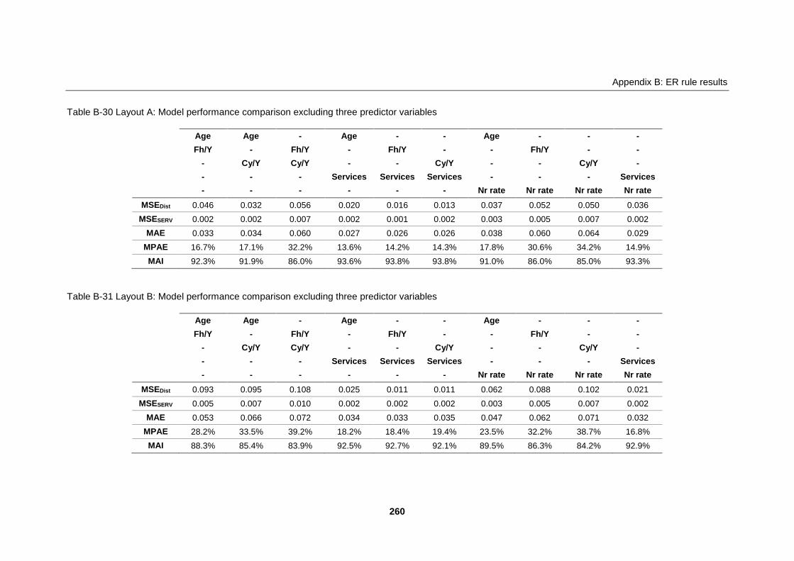
Appendix B: ER rule results
260
Table B-30 Layout A: Model performance comparison excluding three predictor variables
Age Age - Age - - Age - - -
Fh/Y - Fh/Y - Fh/Y - - Fh/Y - -
- Cy/Y Cy/Y - - Cy/Y - - Cy/Y -
- - - Services Services Services - - - Services
- - - - - - Nr rate Nr rate Nr rate Nr rate
MSEDist 0.046 0.032 0.056 0.020 0.016 0.013 0.037 0.052 0.050 0.036
MSESERV 0.002 0.002 0.007 0.002 0.001 0.002 0.003 0.005 0.007 0.002
MAE 0.033 0.034 0.060 0.027 0.026 0.026 0.038 0.060 0.064 0.029
MPAE 16.7% 17.1% 32.2% 13.6% 14.2% 14.3% 17.8% 30.6% 34.2% 14.9%
MAI 92.3% 91.9% 86.0% 93.6% 93.8% 93.8% 91.0% 86.0% 85.0% 93.3%
Table B-31 Layout B: Model performance comparison excluding three predictor variables
Age Age - Age - - Age - - -
Fh/Y - Fh/Y - Fh/Y - - Fh/Y - -
- Cy/Y Cy/Y - - Cy/Y - - Cy/Y -
- - - Services Services Services - - - Services
- - - - - - Nr rate Nr rate Nr rate Nr rate
MSEDist 0.093 0.095 0.108 0.025 0.011 0.011 0.062 0.088 0.102 0.021
MSESERV 0.005 0.007 0.010 0.002 0.002 0.002 0.003 0.005 0.007 0.002
MAE 0.053 0.066 0.072 0.034 0.033 0.035 0.047 0.062 0.071 0.032
MPAE 28.2% 33.5% 39.2% 18.2% 18.4% 19.4% 23.5% 32.2% 38.7% 16.8%
MAI 88.3% 85.4% 83.9% 92.5% 92.7% 92.1% 89.5% 86.3% 84.2% 92.9%

Appendix B: ER rule results
261
B.7 ER rule model scenarios adjusting alpha index, reliability and weight
Table B-32 Layout A (Four samples): Model performance comparison adjusting Alpha index, Reliability and Weight
Sample A Sample B Sample C Sample D
Original
Optimising alphas
R ≠ 1 Optimising
W Original
Optimising alphas
R ≠ 1 Optimising
W Original
Optimising alphas
R ≠ 1 Optimising
W Original
Optimising alphas
R ≠ 1 Optimising
W
Alpha Index 1 Optim Optim Optim 1 Optim Optim Optim 1 Optim Optim Optim 1 Optim Optim Optim
Reliability 1 1 ≠ 1 ≠ 1 1 1 ≠ 1 ≠ 1 1 1 ≠ 1 ≠ 1 1 1 ≠ 1 ≠ 1
Weight 1 1 1 Optim 1 1 1 Optim 1 1 1 Optim 1 1 1 Optim
MSEDIST 0.0128 0.0000 0.0119 0.0000 0.0167 0.0050 0.0159 0.0000
MSESERV 0.0005 0.0004 0.0010 0.0009 0.0006 0.0004 0.0009 0.0006 0.0005 0.0003 0.0008 0.0005 0.0006 0.0004 0.0009 0.0007
MAE 0.0172 0.0155 0.0220 0.0203 0.0179 0.0156 0.0205 0.0167 0.0174 0.0146 0.0204 0.0154 0.0173 0.0155 0.0207 0.0176
MAPE 9.3% 8.0% 10.9% 10.3% 9.7% 8.1% 10.8% 9.1% 8.9% 7.5% 10.2% 7.8% 9.4% 8.1% 10.9% 9.6%
MAI 96.0% 96.3% 94.8% 95.2% 95.8% 96.3% 95.2% 96.1% 95.9% 96.6% 95.2% 96.4% 95.9% 96.4% 95.1% 95.9%
Table B-33 Layout B (Four samples): Model performance comparison adjusting Alpha index, Reliability and Weight
Sample A Sample B Sample C Sample D
Original Optimising
alphas R ≠ 1
Optimising W
Original Optimising
alphas R ≠ 1
Optimising W
Original Optimising
alphas R ≠ 1
Optimising W
Original Optimising
alphas R ≠ 1
Optimising W
Alpha Index 1 Optim Optim Optim 1 Optim Optim Optim 1 Optim Optim Optim 1 Optim Optim Optim
Reliability 1 1 ≠ 1 ≠ 1 1 1 ≠ 1 ≠ 1 1 1 ≠ 1 ≠ 1 1 1 ≠ 1 ≠ 1
Weight 1 1 1 Optim 1 1 1 Optim 1 1 1 Optim 1 1 1 Optim
MSEDIST 0.0049 0.0000 0.0059 0.0000 0.0082 0.0000 0.0061 0.0000
MSESERV 0.0010 0.0010 0.0013 0.0011 0.0009 0.0009 0.0011 0.0008 0.0009 0.0008 0.0011 0.0009 0.0010 0.0010 0.0012 0.0010
MAE 0.0244 0.0240 0.0268 0.0243 0.0242 0.0238 0.0252 0.0195 0.0231 0.0231 0.0244 0.0198 0.0252 0.0249 0.0262 0.0208
MAPE 12.8% 12.9% 13.8% 12.1% 13.5% 13.4% 13.9% 10.3% 12.1% 12.6% 12.8% 9.8% 13.7% 14.0% 14.0% 10.9%
MAI 94.6% 94.7% 94.0% 94.6% 94.6% 94.7% 94.4% 95.7% 94.9% 94.9% 94.6% 95.6% 94.4% 94.5% 94.2% 95.4%

Appendix B: ER rule results
262
B.7.1 Optimised alpha-index results
Table B-34 Layout A, Sample A: Optimised alpha-index per non-routine rate for combining aeroplane age and flight hours per year
Age Fh / Y Alpha-Index per Non-routine rate
0.05-0.1 0.1-0.15 0.15-0.2 0.2-0.25 0.25-0.3 0.3-0.35 0.35-0.4 0.4-0.45 0.45-0.5
4.5-5 3800-3950 0.500 0.500 0.500 0.500 0.500 0.500 0.500 0.500 0.500
5-5.5 3500-3650 0.240 0.625 0.513 0.500 0.500 0.500 0.500 0.500 0.500
5-5.5 3650-3800 0.500 0.500 0.500 0.500 0.500 0.500 0.500 0.500 0.500
5-5.5 4400-4550 0.500 0.500 0.500 0.500 0.500 0.500 0.500 0.500 0.500
5.5-6 3500-3650 0.500 0.627 0.294 0.500 0.500 0.500 0.500 0.500 0.500
5.5-6 3800-3950 0.500 0.237 0.630 0.500 0.500 0.500 0.500 0.500 0.500
5.5-6 3950-4100 0.500 0.500 0.500 0.500 0.500 0.500 0.500 0.500 0.500
6-6.5 3500-3650 0.500 0.541 0.500 0.449 0.500 0.500 0.500 0.500 0.500
6-6.5 3650-3800 0.500 0.428 0.500 0.557 0.500 0.500 0.500 0.500 0.500
7-7.5 3200-3350 0.500 0.500 0.500 0.500 0.500 0.500 0.500 0.500 0.500
7-7.5 3500-3650 0.500 0.500 0.500 0.500 0.500 0.500 0.500 0.500 0.500
7.5-8 3200-3350 0.500 0.500 0.500 0.500 0.500 0.373 0.584 0.500 0.500
7.5-8 3350-3500 0.500 0.500 0.500 0.464 0.534 0.500 0.500 0.500 0.500
7.5-8 3500-3650 0.500 0.500 0.101 0.529 0.658 0.468 0.500 0.500 0.500
8-8.5 3200-3350 0.500 0.500 0.500 0.500 0.500 0.500 0.500 0.500 0.500
9-9.5 2300-2450 0.500 0.500 0.500 0.500 0.500 0.500 0.500 0.500 0.500
9-9.5 3200-3350 0.500 0.500 0.500 0.500 0.500 0.500 0.500 0.500 0.500
9-9.5 3350-3500 0.500 0.500 0.500 0.144 0.659 0.500 0.500 0.500 0.500
9.5-10 3200-3350 0.500 0.500 0.500 0.254 0.500 0.057 0.791 0.349 0.349
9.5-10 3350-3500 0.500 0.500 0.500 0.182 0.638 0.500 0.500 0.500 0.500
9.5-10 3500-3650 0.500 0.500 0.500 0.640 0.131 0.500 0.500 0.500 0.500
9.5-10 3650-3800 0.500 0.500 0.500 0.312 0.606 0.500 0.500 0.500 0.500
10.5-11 3200-3350 0.500 0.500 0.500 0.500 0.500 0.500 0.500 0.500 0.500

Appendix B: ER rule results
263
Age Fh / Y Alpha-Index per Non-routine rate
0.05-0.1 0.1-0.15 0.15-0.2 0.2-0.25 0.25-0.3 0.3-0.35 0.35-0.4 0.4-0.45 0.45-0.5
10.5-11 3800-3950 0.500 0.500 0.500 0.500 0.500 0.500 0.500 0.500 0.500
11-11.5 2900-3050 0.500 0.500 0.500 0.500 0.500 0.500 0.500 0.500 0.500
11-11.5 3800-3950 0.500 0.500 0.500 0.500 0.500 0.500 0.500 0.500 0.500
11.5-12 2900-3050 0.500 0.500 0.500 0.500 0.500 0.500 0.500 0.500 0.500
12.5-13 2900-3050 0.500 0.500 0.500 0.500 0.500 0.500 0.500 0.500 0.500
Table B-35 Layout A, Sample A: Optimised alpha-index per non-routine rate for combining aeroplane age and flight hours per year with cycles per year
Age Fh / Y Cy / Y Alpha-Index per Non-routine rate
0.05-0.1 0.1-0.15 0.15-0.2 0.2-0.25 0.25-0.3 0.3-0.35 0.35-0.4 0.4-0.45 0.45-0.5
4.5-5 3800-3950 1400-1500 0.500 0.500 0.500 0.500 0.500 0.500 0.500 0.500 0.500
4.5-5 3800-3950 1500-1600 0.500 0.500 0.500 0.500 0.500 0.500 0.500 0.500 0.500
5-5.5 3500-3650 1700-1800 0.240 0.625 0.513 0.500 0.500 0.500 0.500 0.500 0.500
5-5.5 3650-3800 1600-1700 0.500 0.500 0.500 0.500 0.500 0.500 0.500 0.500 0.500
5-5.5 4400-4550 1900-2000 0.500 0.500 0.500 0.500 0.500 0.500 0.500 0.500 0.500
5.5-6 3500-3650 1600-1700 0.500 0.634 0.268 0.500 0.500 0.500 0.500 0.500 0.500
5.5-6 3500-3650 1700-1800 0.500 0.490 0.506 0.500 0.500 0.500 0.500 0.500 0.500
5.5-6 3800-3950 1300-1400 0.500 0.500 0.500 0.500 0.500 0.500 0.500 0.500 0.500
5.5-6 3800-3950 1400-1500 0.500 0.237 0.630 0.500 0.500 0.500 0.500 0.500 0.500
5.5-6 3950-4100 1500-1600 0.500 0.500 0.500 0.500 0.500 0.500 0.500 0.500 0.500
5.5-6 3950-4100 1600-1700 0.500 0.500 0.500 0.500 0.500 0.500 0.500 0.500 0.500
6-6.5 3500-3650 1700-1800 0.500 0.541 0.500 0.449 0.500 0.500 0.500 0.500 0.500
6-6.5 3650-3800 1500-1600 0.500 0.090 0.500 0.643 0.500 0.500 0.500 0.500 0.500
6-6.5 3650-3800 1600-1700 0.500 0.613 0.500 0.244 0.500 0.500 0.500 0.500 0.500
7-7.5 3200-3350 1500-1600 0.500 0.500 0.500 0.500 0.500 0.500 0.500 0.500 0.500
7-7.5 3200-3350 1600-1700 0.500 0.500 0.500 0.500 0.500 0.500 0.500 0.500 0.500

Appendix B: ER rule results
264
Age Fh / Y Cy / Y Alpha-Index per Non-routine rate
0.05-0.1 0.1-0.15 0.15-0.2 0.2-0.25 0.25-0.3 0.3-0.35 0.35-0.4 0.4-0.45 0.45-0.5
7-7.5 3200-3350 1700-1800 0.500 0.500 0.500 0.500 0.500 0.500 0.500 0.500 0.500
7-7.5 3500-3650 1600-1700 0.500 0.500 0.500 0.500 0.500 0.500 0.500 0.500 0.500
7.5-8 3200-3350 1600-1700 0.500 0.500 0.500 0.500 0.500 0.096 0.643 0.500 0.500
7.5-8 3200-3350 1700-1800 0.500 0.500 0.500 0.500 0.500 0.592 0.338 0.500 0.500
7.5-8 3200-3350 1800-1900 0.500 0.500 0.500 0.500 0.500 0.500 0.500 0.500 0.500
7.5-8 3350-3500 1600-1700 0.500 0.500 0.500 0.500 0.500 0.500 0.500 0.500 0.500
7.5-8 3350-3500 1700-1800 0.500 0.500 0.500 0.464 0.534 0.500 0.500 0.500 0.500
7.5-8 3350-3500 1800-1900 0.500 0.500 0.500 0.500 0.500 0.500 0.500 0.500 0.500
7.5-8 3500-3650 1600-1700 0.500 0.500 0.101 0.644 0.527 0.468 0.500 0.500 0.500
7.5-8 3500-3650 1700-1800 0.500 0.500 0.500 0.275 0.646 0.500 0.500 0.500 0.500
7.5-8 3500-3650 1800-1900 0.500 0.500 0.500 0.500 0.500 0.500 0.500 0.500 0.500
8-8.5 3200-3350 1600-1700 0.500 0.500 0.500 0.500 0.500 0.500 0.500 0.500 0.500
9-9.5 2300-2450 900-1000 0.500 0.500 0.500 0.500 0.500 0.500 0.500 0.500 0.500
9-9.5 3200-3350 1600-1700 0.500 0.500 0.500 0.500 0.500 0.500 0.500 0.500 0.500
9-9.5 3200-3350 2000-2100 0.500 0.500 0.500 0.500 0.500 0.500 0.500 0.500 0.500
9-9.5 3350-3500 1600-1700 0.500 0.500 0.500 0.348 0.601 0.500 0.500 0.500 0.500
9-9.5 3350-3500 1700-1800 0.500 0.500 0.500 0.366 0.595 0.500 0.500 0.500 0.500
9.5-10 3200-3350 1600-1700 0.500 0.500 0.500 0.406 0.500 0.336 0.706 0.349 0.349
9.5-10 3200-3350 1700-1800 0.500 0.500 0.500 0.368 0.500 0.309 0.678 0.500 0.500
9.5-10 3200-3350 1900-2000 0.500 0.500 0.500 0.500 0.500 0.500 0.500 0.500 0.500
9.5-10 3350-3500 1200-1300 0.500 0.500 0.500 0.182 0.638 0.500 0.500 0.500 0.500
9.5-10 3350-3500 1600-1700 0.500 0.500 0.500 0.500 0.500 0.500 0.500 0.500 0.500
9.5-10 3500-3650 1200-1300 0.500 0.500 0.500 0.640 0.131 0.500 0.500 0.500 0.500
9.5-10 3650-3800 1200-1300 0.500 0.500 0.500 0.312 0.606 0.500 0.500 0.500 0.500
10.5-11 3200-3350 1700-1800 0.500 0.500 0.500 0.500 0.500 0.500 0.500 0.500 0.500
10.5-11 3200-3350 1900-2000 0.500 0.500 0.500 0.500 0.500 0.500 0.500 0.500 0.500

Appendix B: ER rule results
265
Age Fh / Y Cy / Y Alpha-Index per Non-routine rate
0.05-0.1 0.1-0.15 0.15-0.2 0.2-0.25 0.25-0.3 0.3-0.35 0.35-0.4 0.4-0.45 0.45-0.5
10.5-11 3800-3950 2600-2700 0.500 0.500 0.500 0.500 0.500 0.500 0.500 0.500 0.500
11-11.5 2900-3050 1400-1500 0.500 0.500 0.500 0.500 0.500 0.500 0.500 0.500 0.500
11-11.5 3800-3950 2600-2700 0.500 0.500 0.500 0.500 0.500 0.500 0.500 0.500 0.500
11.5-12 2900-3050 1300-1400 0.500 0.500 0.500 0.500 0.500 0.500 0.500 0.500 0.500
11.5-12 2900-3050 1400-1500 0.500 0.500 0.500 0.500 0.500 0.500 0.500 0.500 0.500
12.5-13 2900-3050 1000-1100 0.500 0.500 0.500 0.500 0.500 0.500 0.500 0.500 0.500
Table B-36 Layout A, Sample A: Optimised alpha-index per non-routine rate for combining aeroplane age, flight hours and cycles per year with service type
Age Fh / Y Cy / Y Service Alpha-Index per Non-routine rate
0.05-0.1 0.1-0.15 0.15-0.2 0.2-0.25 0.25-0.3 0.3-0.35 0.35-0.4 0.4-0.45 0.45-0.5
4.5-5 3800-3950 1400-1500 1C 0.500 0.500 0.500 0.500 0.500 0.500 0.500 0.500 0.500
4.5-5 3800-3950 1500-1600 1C 0.500 0.500 0.500 0.500 0.500 0.500 0.500 0.500 0.500
5-5.5 3500-3650 1700-1800 3C 0.500 0.000 0.676 0.500 0.500 0.500 0.500 0.500 0.500
5-5.5 3500-3650 1700-1800 3C+ 0.240 0.726 0.101 0.500 0.500 0.500 0.500 0.500 0.500
5-5.5 3650-3800 1600-1700 3C 0.500 0.500 0.500 0.500 0.500 0.500 0.500 0.500 0.500
5-5.5 4400-4550 1900-2000 3C 0.500 0.500 0.500 0.500 0.500 0.500 0.500 0.500 0.500
5.5-6 3500-3650 1600-1700 3C+ 0.500 0.634 0.268 0.500 0.500 0.500 0.500 0.500 0.500
5.5-6 3500-3650 1700-1800 3C 0.500 0.658 0.044 0.500 0.500 0.500 0.500 0.500 0.500
5.5-6 3500-3650 1700-1800 3C+ 0.500 0.000 0.667 0.500 0.500 0.500 0.500 0.500 0.500
5.5-6 3800-3950 1300-1400 3C+ 0.500 0.500 0.500 0.500 0.500 0.500 0.500 0.500 0.500
5.5-6 3800-3950 1400-1500 3C 0.500 0.237 0.630 0.500 0.500 0.500 0.500 0.500 0.500
5.5-6 3950-4100 1500-1600 3C+ 0.500 0.500 0.500 0.500 0.500 0.500 0.500 0.500 0.500
5.5-6 3950-4100 1600-1700 3C 0.500 0.500 0.500 0.500 0.500 0.500 0.500 0.500 0.500
6-6.5 3500-3650 1700-1800 2C 0.500 0.541 0.500 0.449 0.500 0.500 0.500 0.500 0.500
6-6.5 3650-3800 1500-1600 1C 0.500 0.500 0.500 0.500 0.500 0.500 0.500 0.500 0.500

Appendix B: ER rule results
266
Age Fh / Y Cy / Y Service Alpha-Index per Non-routine rate
0.05-0.1 0.1-0.15 0.15-0.2 0.2-0.25 0.25-0.3 0.3-0.35 0.35-0.4 0.4-0.45 0.45-0.5
6-6.5 3650-3800 1500-1600 2C 0.500 0.090 0.500 0.643 0.500 0.500 0.500 0.500 0.500
6-6.5 3650-3800 1600-1700 2C 0.500 0.613 0.500 0.244 0.500 0.500 0.500 0.500 0.500
7-7.5 3200-3350 1500-1600 1C 0.500 0.500 0.500 0.500 0.500 0.500 0.500 0.500 0.500
7-7.5 3200-3350 1600-1700 1C 0.500 0.500 0.500 0.500 0.500 0.500 0.500 0.500 0.500
7-7.5 3200-3350 1700-1800 1C 0.500 0.500 0.500 0.500 0.500 0.500 0.500 0.500 0.500
7-7.5 3500-3650 1600-1700 2C 0.500 0.500 0.500 0.500 0.500 0.500 0.500 0.500 0.500
7.5-8 3200-3350 1600-1700 4C 0.500 0.500 0.500 0.500 0.500 0.096 0.643 0.500 0.500
7.5-8 3200-3350 1700-1800 1C 0.500 0.500 0.500 0.500 0.500 0.500 0.500 0.500 0.500
7.5-8 3200-3350 1700-1800 4C 0.500 0.500 0.500 0.500 0.500 0.592 0.338 0.500 0.500
7.5-8 3200-3350 1700-1800 4C+ 0.500 0.500 0.500 0.500 0.500 0.500 0.500 0.500 0.500
7.5-8 3200-3350 1800-1900 4C 0.500 0.500 0.500 0.500 0.500 0.500 0.500 0.500 0.500
7.5-8 3350-3500 1600-1700 1C 0.500 0.500 0.500 0.500 0.500 0.500 0.500 0.500 0.500
7.5-8 3350-3500 1600-1700 4C 0.500 0.500 0.500 0.500 0.500 0.500 0.500 0.500 0.500
7.5-8 3350-3500 1700-1800 4C+ 0.500 0.500 0.500 0.464 0.534 0.500 0.500 0.500 0.500
7.5-8 3350-3500 1800-1900 4C+ 0.500 0.500 0.500 0.500 0.500 0.500 0.500 0.500 0.500
7.5-8 3500-3650 1600-1700 3C+ 0.500 0.500 0.101 0.644 0.500 0.500 0.500 0.500 0.500
7.5-8 3500-3650 1600-1700 4C 0.500 0.500 0.500 0.500 0.527 0.468 0.500 0.500 0.500
7.5-8 3500-3650 1700-1800 4C+ 0.500 0.500 0.500 0.275 0.646 0.500 0.500 0.500 0.500
7.5-8 3500-3650 1800-1900 4C+ 0.500 0.500 0.500 0.500 0.500 0.500 0.500 0.500 0.500
8-8.5 3200-3350 1600-1700 4C 0.500 0.500 0.500 0.500 0.500 0.500 0.500 0.500 0.500
9-9.5 2300-2450 900-1000 2C 0.500 0.500 0.500 0.500 0.500 0.500 0.500 0.500 0.500
9-9.5 3200-3350 1600-1700 2C 0.500 0.500 0.500 0.500 0.500 0.500 0.500 0.500 0.500
9-9.5 3200-3350 2000-2100 5C+ 0.500 0.500 0.500 0.500 0.500 0.500 0.500 0.500 0.500
9-9.5 3350-3500 1600-1700 2C 0.500 0.500 0.500 0.348 0.601 0.500 0.500 0.500 0.500
9-9.5 3350-3500 1700-1800 2C 0.500 0.500 0.500 0.366 0.595 0.500 0.500 0.500 0.500
9.5-10 3200-3350 1600-1700 5C 0.500 0.500 0.500 0.406 0.500 0.336 0.706 0.349 0.349
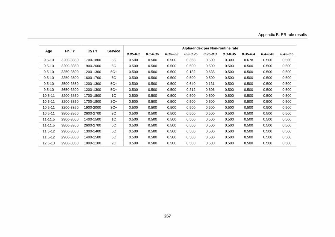
Appendix B: ER rule results
267
Age Fh / Y Cy / Y Service Alpha-Index per Non-routine rate
0.05-0.1 0.1-0.15 0.15-0.2 0.2-0.25 0.25-0.3 0.3-0.35 0.35-0.4 0.4-0.45 0.45-0.5
9.5-10 3200-3350 1700-1800 5C 0.500 0.500 0.500 0.368 0.500 0.309 0.678 0.500 0.500
9.5-10 3200-3350 1900-2000 5C 0.500 0.500 0.500 0.500 0.500 0.500 0.500 0.500 0.500
9.5-10 3350-3500 1200-1300 5C+ 0.500 0.500 0.500 0.182 0.638 0.500 0.500 0.500 0.500
9.5-10 3350-3500 1600-1700 5C 0.500 0.500 0.500 0.500 0.500 0.500 0.500 0.500 0.500
9.5-10 3500-3650 1200-1300 5C+ 0.500 0.500 0.500 0.640 0.131 0.500 0.500 0.500 0.500
9.5-10 3650-3800 1200-1300 5C+ 0.500 0.500 0.500 0.312 0.606 0.500 0.500 0.500 0.500
10.5-11 3200-3350 1700-1800 1C 0.500 0.500 0.500 0.500 0.500 0.500 0.500 0.500 0.500
10.5-11 3200-3350 1700-1800 3C+ 0.500 0.500 0.500 0.500 0.500 0.500 0.500 0.500 0.500
10.5-11 3200-3350 1900-2000 3C+ 0.500 0.500 0.500 0.500 0.500 0.500 0.500 0.500 0.500
10.5-11 3800-3950 2600-2700 3C 0.500 0.500 0.500 0.500 0.500 0.500 0.500 0.500 0.500
11-11.5 2900-3050 1400-1500 1C 0.500 0.500 0.500 0.500 0.500 0.500 0.500 0.500 0.500
11-11.5 3800-3950 2600-2700 6C 0.500 0.500 0.500 0.500 0.500 0.500 0.500 0.500 0.500
11.5-12 2900-3050 1300-1400 6C 0.500 0.500 0.500 0.500 0.500 0.500 0.500 0.500 0.500
11.5-12 2900-3050 1400-1500 6C 0.500 0.500 0.500 0.500 0.500 0.500 0.500 0.500 0.500
12.5-13 2900-3050 1000-1100 2C 0.500 0.500 0.500 0.500 0.500 0.500 0.500 0.500 0.500

Appendix B: ER rule results
268
Table B-37 Layout A, Sample B: Optimised alpha-index per non-routine rate for combining aeroplane age and flight hours per year
Age Fh / Y Alpha-Index per Non-routine rate
0.05-0.1 0.1-0.15 0.15-0.2 0.2-0.25 0.25-0.3 0.3-0.35 0.35-0.4 0.4-0.45 0.45-0.5
4.5-5 3800-3950 0.501 0.501 0.501 0.501 0.501 0.501 0.501 0.501 0.501
5-5.5 3500-3650 0.299 0.609 0.501 0.501 0.501 0.501 0.501 0.501 0.501
5-5.5 3650-3800 0.501 0.501 0.501 0.501 0.501 0.501 0.501 0.501 0.501
5-5.5 4400-4550 0.501 0.501 0.501 0.501 0.501 0.501 0.501 0.501 0.501
5.5-6 3500-3650 0.501 0.493 0.630 0.297 0.501 0.501 0.501 0.501 0.501
5.5-6 3800-3950 0.501 0.311 0.633 0.455 0.501 0.501 0.501 0.501 0.501
5.5-6 3950-4100 0.501 0.302 0.501 0.609 0.501 0.501 0.501 0.501 0.501
6-6.5 3500-3650 0.501 0.520 0.501 0.482 0.501 0.501 0.501 0.501 0.501
6-6.5 3650-3800 0.501 0.445 0.501 0.553 0.501 0.501 0.501 0.501 0.501
7-7.5 3200-3350 0.501 0.501 0.501 0.501 0.501 0.501 0.501 0.501 0.501
7-7.5 3500-3650 0.501 0.501 0.501 0.501 0.501 0.501 0.501 0.501 0.501
7.5-8 3200-3350 0.501 0.501 0.501 0.501 0.098 0.490 0.702 0.501 0.501
7.5-8 3350-3500 0.501 0.501 0.501 0.501 0.501 0.501 0.501 0.501 0.501
7.5-8 3500-3650 0.501 0.501 0.130 0.651 0.501 0.501 0.501 0.501 0.501
8-8.5 3200-3350 0.501 0.501 0.501 0.501 0.501 0.501 0.501 0.501 0.501
9-9.5 2300-2450 0.501 0.501 0.501 0.501 0.501 0.501 0.501 0.501 0.501
9-9.5 3200-3350 0.501 0.501 0.501 0.586 0.360 0.501 0.501 0.501 0.501
9-9.5 3350-3500 0.501 0.501 0.501 0.241 0.667 0.501 0.501 0.501 0.501
9.5-10 3200-3350 0.501 0.501 0.501 0.437 0.501 0.040 0.751 0.354 0.355
9.5-10 3350-3500 0.501 0.501 0.501 0.147 0.650 0.501 0.501 0.501 0.501
9.5-10 3500-3650 0.501 0.501 0.501 0.650 0.146 0.501 0.501 0.501 0.501
9.5-10 3650-3800 0.501 0.501 0.501 0.288 0.611 0.501 0.501 0.501 0.501
10-10.5 2900-3050 0.501 0.501 0.501 0.501 0.501 0.501 0.501 0.501 0.501
10-10.5 3500-3650 0.501 0.501 0.501 0.501 0.501 0.501 0.501 0.501 0.501

Appendix B: ER rule results
269
Age Fh / Y Alpha-Index per Non-routine rate
0.05-0.1 0.1-0.15 0.15-0.2 0.2-0.25 0.25-0.3 0.3-0.35 0.35-0.4 0.4-0.45 0.45-0.5
10.5-11 3200-3350 0.501 0.501 0.501 0.501 0.501 0.501 0.501 0.501 0.501
11-11.5 2900-3050 0.501 0.501 0.501 0.501 0.501 0.501 0.501 0.501 0.501
11-11.5 3800-3950 0.501 0.501 0.501 0.501 0.501 0.501 0.501 0.501 0.501
11.5-12 2900-3050 0.501 0.501 0.501 0.501 0.501 0.501 0.501 0.501 0.501
12.5-13 2900-3050 0.501 0.501 0.501 0.501 0.501 0.501 0.501 0.501 0.501
Table B-38 Layout A, Sample B: Optimised alpha-index per non-routine rate for combining aeroplane age and flight hours per year with cycles per year
Age Fh / Y Cy / Y Alpha-Index per Non-routine rate
0.05-0.1 0.1-0.15 0.15-0.2 0.2-0.25 0.25-0.3 0.3-0.35 0.35-0.4 0.4-0.45 0.45-0.5
4.5-5 3800-3950 1400-1500 0.501 0.501 0.501 0.501 0.501 0.501 0.501 0.501 0.501
4.5-5 3800-3950 1500-1600 0.501 0.501 0.501 0.501 0.501 0.501 0.501 0.501 0.501
5-5.5 3500-3650 1600-1700 0.501 0.501 0.501 0.501 0.501 0.501 0.501 0.501 0.501
5-5.5 3500-3650 1700-1800 0.299 0.609 0.501 0.501 0.501 0.501 0.501 0.501 0.501
5-5.5 3500-3650 1800-1900 0.501 0.501 0.501 0.501 0.501 0.501 0.501 0.501 0.501
5-5.5 3650-3800 1600-1700 0.501 0.501 0.501 0.501 0.501 0.501 0.501 0.501 0.501
5-5.5 4400-4550 1900-2000 0.501 0.501 0.501 0.501 0.501 0.501 0.501 0.501 0.501
5.5-6 3500-3650 1700-1800 0.501 0.493 0.630 0.297 0.501 0.501 0.501 0.501 0.501
5.5-6 3800-3950 1300-1400 0.501 0.545 0.501 0.455 0.501 0.501 0.501 0.501 0.501
5.5-6 3800-3950 1400-1500 0.501 0.218 0.633 0.501 0.501 0.501 0.501 0.501 0.501
5.5-6 3950-4100 1400-1500 0.501 0.032 0.501 0.664 0.501 0.501 0.501 0.501 0.501
5.5-6 3950-4100 1500-1600 0.501 0.588 0.501 0.395 0.501 0.501 0.501 0.501 0.501
5.5-6 3950-4100 1600-1700 0.501 0.501 0.501 0.501 0.501 0.501 0.501 0.501 0.501
6-6.5 3500-3650 1700-1800 0.501 0.520 0.501 0.482 0.501 0.501 0.501 0.501 0.501
6-6.5 3650-3800 1500-1600 0.501 0.094 0.501 0.652 0.501 0.501 0.501 0.501 0.501
6-6.5 3650-3800 1600-1700 0.501 0.629 0.501 0.206 0.501 0.501 0.501 0.501 0.501

Appendix B: ER rule results
270
Age Fh / Y Cy / Y Alpha-Index per Non-routine rate
0.05-0.1 0.1-0.15 0.15-0.2 0.2-0.25 0.25-0.3 0.3-0.35 0.35-0.4 0.4-0.45 0.45-0.5
7-7.5 3200-3350 1500-1600 0.501 0.501 0.501 0.501 0.501 0.501 0.501 0.501 0.501
7-7.5 3200-3350 1600-1700 0.501 0.501 0.501 0.501 0.501 0.501 0.501 0.501 0.501
7-7.5 3200-3350 1700-1800 0.501 0.501 0.501 0.501 0.501 0.501 0.501 0.501 0.501
7-7.5 3500-3650 1600-1700 0.501 0.501 0.501 0.501 0.501 0.501 0.501 0.501 0.501
7.5-8 3200-3350 1600-1700 0.501 0.501 0.501 0.501 0.352 0.148 0.693 0.501 0.501
7.5-8 3200-3350 1700-1800 0.501 0.501 0.501 0.501 0.426 0.645 0.304 0.501 0.501
7.5-8 3200-3350 1800-1900 0.501 0.501 0.501 0.501 0.414 0.501 0.574 0.501 0.501
7.5-8 3350-3500 1600-1700 0.501 0.501 0.501 0.501 0.501 0.501 0.501 0.501 0.501
7.5-8 3350-3500 1700-1800 0.501 0.501 0.501 0.501 0.501 0.501 0.501 0.501 0.501
7.5-8 3350-3500 1800-1900 0.501 0.501 0.501 0.501 0.501 0.501 0.501 0.501 0.501
7.5-8 3500-3650 1600-1700 0.501 0.501 0.130 0.651 0.501 0.501 0.501 0.501 0.501
7.5-8 3500-3650 1700-1800 0.501 0.501 0.501 0.501 0.501 0.501 0.501 0.501 0.501
7.5-8 3500-3650 1800-1900 0.501 0.501 0.501 0.501 0.501 0.501 0.501 0.501 0.501
8-8.5 3200-3350 1600-1700 0.501 0.501 0.501 0.501 0.501 0.501 0.501 0.501 0.501
9-9.5 2300-2450 900-1000 0.501 0.501 0.501 0.501 0.501 0.501 0.501 0.501 0.501
9-9.5 3200-3350 1600-1700 0.501 0.501 0.501 0.561 0.418 0.501 0.501 0.501 0.501
9-9.5 3200-3350 2000-2100 0.501 0.501 0.501 0.535 0.460 0.501 0.501 0.501 0.501
9-9.5 3350-3500 1600-1700 0.501 0.501 0.501 0.347 0.614 0.501 0.501 0.501 0.501
9-9.5 3350-3500 1700-1800 0.501 0.501 0.501 0.423 0.570 0.501 0.501 0.501 0.501
9.5-10 3200-3350 1600-1700 0.501 0.501 0.501 0.461 0.501 0.348 0.688 0.354 0.355
9.5-10 3200-3350 1700-1800 0.501 0.501 0.501 0.478 0.501 0.289 0.629 0.501 0.501
9.5-10 3200-3350 1900-2000 0.501 0.501 0.501 0.501 0.501 0.501 0.501 0.501 0.501
9.5-10 3350-3500 1200-1300 0.501 0.501 0.501 0.147 0.650 0.501 0.501 0.501 0.501
9.5-10 3350-3500 1600-1700 0.501 0.501 0.501 0.501 0.501 0.501 0.501 0.501 0.501
9.5-10 3500-3650 1200-1300 0.501 0.501 0.501 0.650 0.146 0.501 0.501 0.501 0.501
9.5-10 3650-3800 1200-1300 0.501 0.501 0.501 0.288 0.611 0.501 0.501 0.501 0.501

Appendix B: ER rule results
271
Age Fh / Y Cy / Y Alpha-Index per Non-routine rate
0.05-0.1 0.1-0.15 0.15-0.2 0.2-0.25 0.25-0.3 0.3-0.35 0.35-0.4 0.4-0.45 0.45-0.5
10-10.5 2900-3050 1400-1500 0.501 0.501 0.501 0.501 0.501 0.501 0.501 0.501 0.501
10-10.5 3500-3650 1900-2000 0.501 0.501 0.501 0.501 0.501 0.501 0.501 0.501 0.501
10.5-11 3200-3350 1700-1800 0.501 0.501 0.501 0.501 0.501 0.501 0.501 0.501 0.501
10.5-11 3200-3350 1900-2000 0.501 0.501 0.501 0.501 0.501 0.501 0.501 0.501 0.501
11-11.5 2900-3050 1400-1500 0.501 0.501 0.501 0.501 0.501 0.501 0.501 0.501 0.501
11-11.5 3800-3950 2600-2700 0.501 0.501 0.501 0.501 0.501 0.501 0.501 0.501 0.501
11.5-12 2900-3050 1300-1400 0.501 0.501 0.501 0.501 0.501 0.501 0.501 0.501 0.501
12.5-13 2900-3050 1000-1100 0.501 0.501 0.501 0.501 0.501 0.501 0.501 0.501 0.501
Table B-39 Layout A, Sample B: Optimised alpha-index per non-routine rate for combining aeroplane age, flight hours and cycles per year with service type
Age Fh / Y Cy / Y Service Alpha-Index per Non-routine rate
0.05-0.1 0.1-0.15 0.15-0.2 0.2-0.25 0.25-0.3 0.3-0.35 0.35-0.4 0.4-0.45 0.45-0.5
4.5-5 3800-3950 1400-1500 1C 0.501 0.501 0.501 0.501 0.501 0.501 0.501 0.501 0.501
4.5-5 3800-3950 1500-1600 1C 0.501 0.501 0.501 0.501 0.501 0.501 0.501 0.501 0.501
5-5.5 3500-3650 1600-1700 3C+ 0.501 0.501 0.501 0.501 0.501 0.501 0.501 0.501 0.501
5-5.5 3500-3650 1700-1800 3C+ 0.299 0.609 0.501 0.501 0.501 0.501 0.501 0.501 0.501
5-5.5 3500-3650 1800-1900 3C+ 0.501 0.501 0.501 0.501 0.501 0.501 0.501 0.501 0.501
5-5.5 3650-3800 1600-1700 3C 0.501 0.501 0.501 0.501 0.501 0.501 0.501 0.501 0.501
5-5.5 4400-4550 1900-2000 3C 0.501 0.501 0.501 0.501 0.501 0.501 0.501 0.501 0.501
5.5-6 3500-3650 1700-1800 3C 0.501 0.660 0.017 0.501 0.501 0.501 0.501 0.501 0.501
5.5-6 3500-3650 1700-1800 3C+ 0.501 0.001 0.732 0.297 0.501 0.501 0.501 0.501 0.501
5.5-6 3800-3950 1300-1400 3C+ 0.501 0.545 0.501 0.455 0.501 0.501 0.501 0.501 0.501
5.5-6 3800-3950 1400-1500 3C 0.501 0.218 0.633 0.501 0.501 0.501 0.501 0.501 0.501
5.5-6 3950-4100 1400-1500 2C 0.501 0.032 0.501 0.664 0.501 0.501 0.501 0.501 0.501
5.5-6 3950-4100 1500-1600 3C+ 0.501 0.588 0.501 0.395 0.501 0.501 0.501 0.501 0.501

Appendix B: ER rule results
272
Age Fh / Y Cy / Y Service Alpha-Index per Non-routine rate
0.05-0.1 0.1-0.15 0.15-0.2 0.2-0.25 0.25-0.3 0.3-0.35 0.35-0.4 0.4-0.45 0.45-0.5
5.5-6 3950-4100 1600-1700 3C 0.501 0.501 0.501 0.501 0.501 0.501 0.501 0.501 0.501
6-6.5 3500-3650 1700-1800 2C 0.501 0.520 0.501 0.482 0.501 0.501 0.501 0.501 0.501
6-6.5 3650-3800 1500-1600 1C 0.501 0.501 0.501 0.501 0.501 0.501 0.501 0.501 0.501
6-6.5 3650-3800 1500-1600 2C 0.501 0.094 0.501 0.652 0.501 0.501 0.501 0.501 0.501
6-6.5 3650-3800 1600-1700 2C 0.501 0.629 0.501 0.206 0.501 0.501 0.501 0.501 0.501
7-7.5 3200-3350 1500-1600 1C 0.501 0.501 0.501 0.501 0.501 0.501 0.501 0.501 0.501
7-7.5 3200-3350 1600-1700 1C 0.501 0.501 0.501 0.501 0.501 0.501 0.501 0.501 0.501
7-7.5 3200-3350 1700-1800 1C 0.501 0.501 0.501 0.501 0.501 0.501 0.501 0.501 0.501
7-7.5 3500-3650 1600-1700 2C 0.501 0.501 0.501 0.501 0.501 0.501 0.501 0.501 0.501
7.5-8 3200-3350 1600-1700 4C 0.501 0.501 0.501 0.501 0.352 0.148 0.693 0.501 0.501
7.5-8 3200-3350 1700-1800 1C 0.501 0.501 0.501 0.501 0.501 0.501 0.501 0.501 0.501
7.5-8 3200-3350 1700-1800 4C 0.501 0.501 0.501 0.501 0.426 0.645 0.304 0.501 0.501
7.5-8 3200-3350 1700-1800 4C+ 0.501 0.501 0.501 0.501 0.501 0.501 0.501 0.501 0.501
7.5-8 3200-3350 1800-1900 4C 0.501 0.501 0.501 0.501 0.414 0.501 0.574 0.501 0.501
7.5-8 3350-3500 1600-1700 4C 0.501 0.501 0.501 0.501 0.501 0.501 0.501 0.501 0.501
7.5-8 3350-3500 1700-1800 4C+ 0.501 0.501 0.501 0.501 0.501 0.501 0.501 0.501 0.501
7.5-8 3350-3500 1800-1900 4C+ 0.501 0.501 0.501 0.501 0.501 0.501 0.501 0.501 0.501
7.5-8 3500-3650 1600-1700 3C+ 0.501 0.501 0.130 0.651 0.501 0.501 0.501 0.501 0.501
7.5-8 3500-3650 1600-1700 4C 0.501 0.501 0.501 0.501 0.501 0.501 0.501 0.501 0.501
7.5-8 3500-3650 1700-1800 4C+ 0.501 0.501 0.501 0.501 0.501 0.501 0.501 0.501 0.501
7.5-8 3500-3650 1800-1900 4C+ 0.501 0.501 0.501 0.501 0.501 0.501 0.501 0.501 0.501
8-8.5 3200-3350 1600-1700 4C 0.501 0.501 0.501 0.501 0.501 0.501 0.501 0.501 0.501
9-9.5 2300-2450 900-1000 2C 0.501 0.501 0.501 0.501 0.501 0.501 0.501 0.501 0.501
9-9.5 3200-3350 1600-1700 2C 0.501 0.501 0.501 0.561 0.418 0.501 0.501 0.501 0.501
9-9.5 3200-3350 2000-2100 5C+ 0.501 0.501 0.501 0.535 0.460 0.501 0.501 0.501 0.501
9-9.5 3350-3500 1600-1700 2C 0.501 0.501 0.501 0.347 0.614 0.501 0.501 0.501 0.501

Appendix B: ER rule results
273
Age Fh / Y Cy / Y Service Alpha-Index per Non-routine rate
0.05-0.1 0.1-0.15 0.15-0.2 0.2-0.25 0.25-0.3 0.3-0.35 0.35-0.4 0.4-0.45 0.45-0.5
9-9.5 3350-3500 1700-1800 2C 0.501 0.501 0.501 0.423 0.570 0.501 0.501 0.501 0.501
9.5-10 3200-3350 1600-1700 5C 0.501 0.501 0.501 0.461 0.501 0.348 0.688 0.354 0.355
9.5-10 3200-3350 1700-1800 5C 0.501 0.501 0.501 0.478 0.501 0.289 0.629 0.501 0.501
9.5-10 3200-3350 1900-2000 5C 0.501 0.501 0.501 0.501 0.501 0.501 0.501 0.501 0.501
9.5-10 3350-3500 1200-1300 5C+ 0.501 0.501 0.501 0.147 0.650 0.501 0.501 0.501 0.501
9.5-10 3350-3500 1600-1700 5C 0.501 0.501 0.501 0.501 0.501 0.501 0.501 0.501 0.501
9.5-10 3500-3650 1200-1300 5C+ 0.501 0.501 0.501 0.650 0.146 0.501 0.501 0.501 0.501
9.5-10 3650-3800 1200-1300 5C+ 0.501 0.501 0.501 0.288 0.611 0.501 0.501 0.501 0.501
10-10.5 2900-3050 1400-1500 3C+ 0.501 0.501 0.501 0.501 0.501 0.501 0.501 0.501 0.501
10-10.5 3500-3650 1900-2000 3C+ 0.501 0.501 0.501 0.501 0.501 0.501 0.501 0.501 0.501
10.5-11 3200-3350 1700-1800 1C 0.501 0.501 0.501 0.501 0.501 0.501 0.501 0.501 0.501
10.5-11 3200-3350 1700-1800 3C+ 0.501 0.501 0.501 0.501 0.501 0.501 0.501 0.501 0.501
10.5-11 3200-3350 1900-2000 3C+ 0.501 0.501 0.501 0.501 0.501 0.501 0.501 0.501 0.501
11-11.5 2900-3050 1400-1500 1C 0.501 0.501 0.501 0.501 0.501 0.501 0.501 0.501 0.501
11-11.5 3800-3950 2600-2700 6C 0.501 0.501 0.501 0.501 0.501 0.501 0.501 0.501 0.501
11.5-12 2900-3050 1300-1400 6C 0.501 0.501 0.501 0.501 0.501 0.501 0.501 0.501 0.501
12.5-13 2900-3050 1000-1100 2C 0.501 0.501 0.501 0.501 0.501 0.501 0.501 0.501 0.501
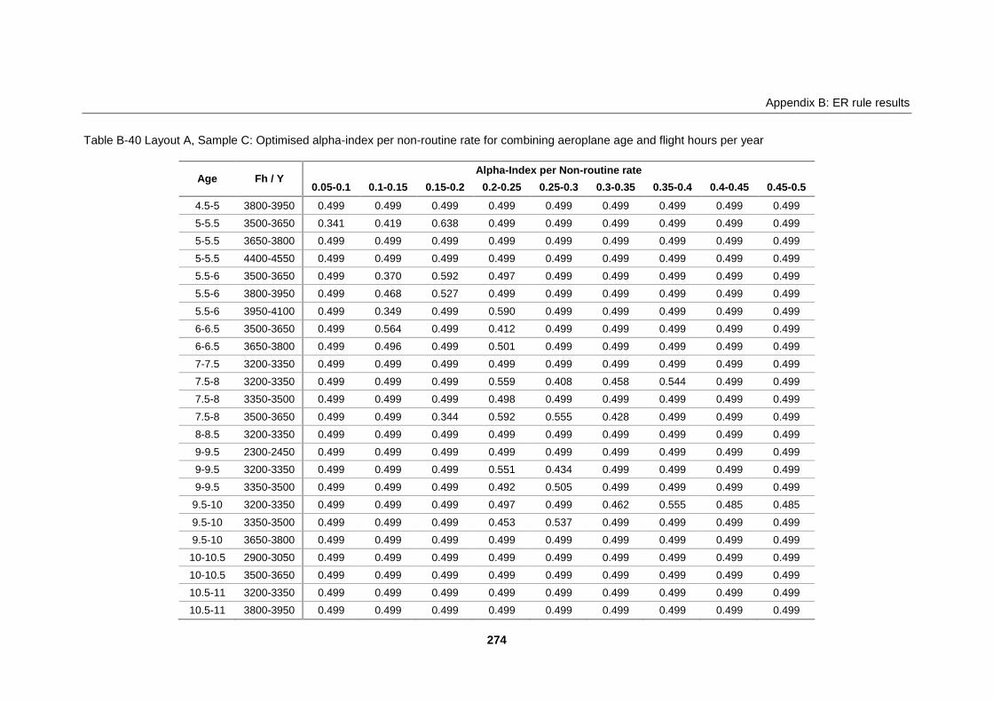
Appendix B: ER rule results
274
Table B-40 Layout A, Sample C: Optimised alpha-index per non-routine rate for combining aeroplane age and flight hours per year
Age Fh / Y Alpha-Index per Non-routine rate
0.05-0.1 0.1-0.15 0.15-0.2 0.2-0.25 0.25-0.3 0.3-0.35 0.35-0.4 0.4-0.45 0.45-0.5
4.5-5 3800-3950 0.499 0.499 0.499 0.499 0.499 0.499 0.499 0.499 0.499
5-5.5 3500-3650 0.341 0.419 0.638 0.499 0.499 0.499 0.499 0.499 0.499
5-5.5 3650-3800 0.499 0.499 0.499 0.499 0.499 0.499 0.499 0.499 0.499
5-5.5 4400-4550 0.499 0.499 0.499 0.499 0.499 0.499 0.499 0.499 0.499
5.5-6 3500-3650 0.499 0.370 0.592 0.497 0.499 0.499 0.499 0.499 0.499
5.5-6 3800-3950 0.499 0.468 0.527 0.499 0.499 0.499 0.499 0.499 0.499
5.5-6 3950-4100 0.499 0.349 0.499 0.590 0.499 0.499 0.499 0.499 0.499
6-6.5 3500-3650 0.499 0.564 0.499 0.412 0.499 0.499 0.499 0.499 0.499
6-6.5 3650-3800 0.499 0.496 0.499 0.501 0.499 0.499 0.499 0.499 0.499
7-7.5 3200-3350 0.499 0.499 0.499 0.499 0.499 0.499 0.499 0.499 0.499
7.5-8 3200-3350 0.499 0.499 0.499 0.559 0.408 0.458 0.544 0.499 0.499
7.5-8 3350-3500 0.499 0.499 0.499 0.498 0.499 0.499 0.499 0.499 0.499
7.5-8 3500-3650 0.499 0.499 0.344 0.592 0.555 0.428 0.499 0.499 0.499
8-8.5 3200-3350 0.499 0.499 0.499 0.499 0.499 0.499 0.499 0.499 0.499
9-9.5 2300-2450 0.499 0.499 0.499 0.499 0.499 0.499 0.499 0.499 0.499
9-9.5 3200-3350 0.499 0.499 0.499 0.551 0.434 0.499 0.499 0.499 0.499
9-9.5 3350-3500 0.499 0.499 0.499 0.492 0.505 0.499 0.499 0.499 0.499
9.5-10 3200-3350 0.499 0.499 0.499 0.497 0.499 0.462 0.555 0.485 0.485
9.5-10 3350-3500 0.499 0.499 0.499 0.453 0.537 0.499 0.499 0.499 0.499
9.5-10 3650-3800 0.499 0.499 0.499 0.499 0.499 0.499 0.499 0.499 0.499
10-10.5 2900-3050 0.499 0.499 0.499 0.499 0.499 0.499 0.499 0.499 0.499
10-10.5 3500-3650 0.499 0.499 0.499 0.499 0.499 0.499 0.499 0.499 0.499
10.5-11 3200-3350 0.499 0.499 0.499 0.499 0.499 0.499 0.499 0.499 0.499
10.5-11 3800-3950 0.499 0.499 0.499 0.499 0.499 0.499 0.499 0.499 0.499
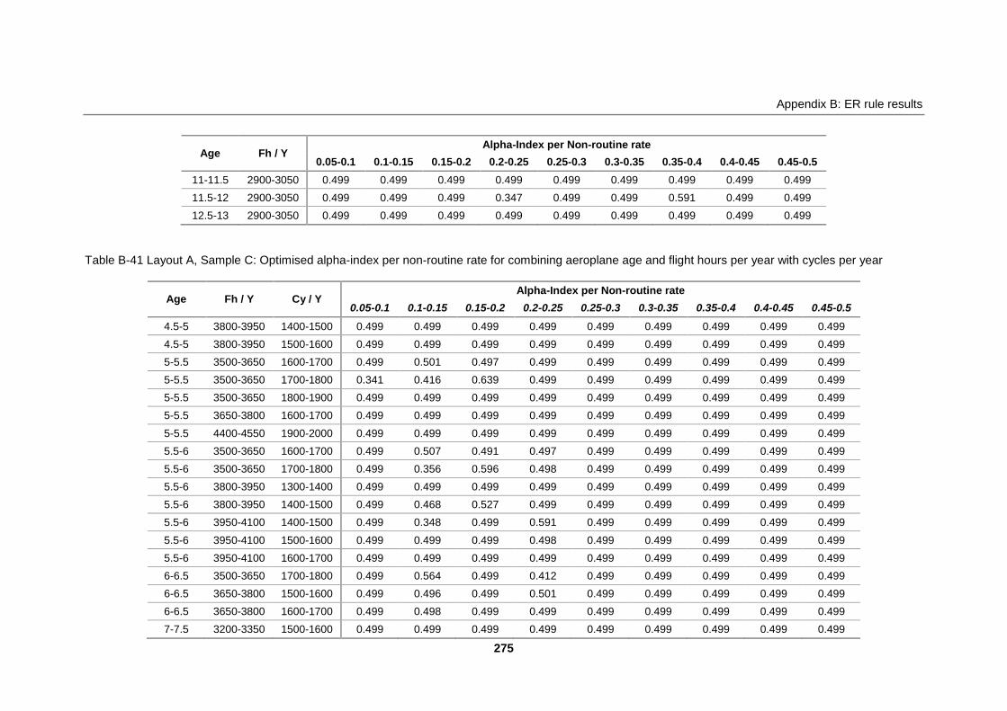
Appendix B: ER rule results
275
Age Fh / Y Alpha-Index per Non-routine rate
0.05-0.1 0.1-0.15 0.15-0.2 0.2-0.25 0.25-0.3 0.3-0.35 0.35-0.4 0.4-0.45 0.45-0.5
11-11.5 2900-3050 0.499 0.499 0.499 0.499 0.499 0.499 0.499 0.499 0.499
11.5-12 2900-3050 0.499 0.499 0.499 0.347 0.499 0.499 0.591 0.499 0.499
12.5-13 2900-3050 0.499 0.499 0.499 0.499 0.499 0.499 0.499 0.499 0.499
Table B-41 Layout A, Sample C: Optimised alpha-index per non-routine rate for combining aeroplane age and flight hours per year with cycles per year
Age Fh / Y Cy / Y Alpha-Index per Non-routine rate
0.05-0.1 0.1-0.15 0.15-0.2 0.2-0.25 0.25-0.3 0.3-0.35 0.35-0.4 0.4-0.45 0.45-0.5
4.5-5 3800-3950 1400-1500 0.499 0.499 0.499 0.499 0.499 0.499 0.499 0.499 0.499
4.5-5 3800-3950 1500-1600 0.499 0.499 0.499 0.499 0.499 0.499 0.499 0.499 0.499
5-5.5 3500-3650 1600-1700 0.499 0.501 0.497 0.499 0.499 0.499 0.499 0.499 0.499
5-5.5 3500-3650 1700-1800 0.341 0.416 0.639 0.499 0.499 0.499 0.499 0.499 0.499
5-5.5 3500-3650 1800-1900 0.499 0.499 0.499 0.499 0.499 0.499 0.499 0.499 0.499
5-5.5 3650-3800 1600-1700 0.499 0.499 0.499 0.499 0.499 0.499 0.499 0.499 0.499
5-5.5 4400-4550 1900-2000 0.499 0.499 0.499 0.499 0.499 0.499 0.499 0.499 0.499
5.5-6 3500-3650 1600-1700 0.499 0.507 0.491 0.497 0.499 0.499 0.499 0.499 0.499
5.5-6 3500-3650 1700-1800 0.499 0.356 0.596 0.498 0.499 0.499 0.499 0.499 0.499
5.5-6 3800-3950 1300-1400 0.499 0.499 0.499 0.499 0.499 0.499 0.499 0.499 0.499
5.5-6 3800-3950 1400-1500 0.499 0.468 0.527 0.499 0.499 0.499 0.499 0.499 0.499
5.5-6 3950-4100 1400-1500 0.499 0.348 0.499 0.591 0.499 0.499 0.499 0.499 0.499
5.5-6 3950-4100 1500-1600 0.499 0.499 0.499 0.498 0.499 0.499 0.499 0.499 0.499
5.5-6 3950-4100 1600-1700 0.499 0.499 0.499 0.499 0.499 0.499 0.499 0.499 0.499
6-6.5 3500-3650 1700-1800 0.499 0.564 0.499 0.412 0.499 0.499 0.499 0.499 0.499
6-6.5 3650-3800 1500-1600 0.499 0.496 0.499 0.501 0.499 0.499 0.499 0.499 0.499
6-6.5 3650-3800 1600-1700 0.499 0.498 0.499 0.499 0.499 0.499 0.499 0.499 0.499
7-7.5 3200-3350 1500-1600 0.499 0.499 0.499 0.499 0.499 0.499 0.499 0.499 0.499

Appendix B: ER rule results
276
Age Fh / Y Cy / Y Alpha-Index per Non-routine rate
0.05-0.1 0.1-0.15 0.15-0.2 0.2-0.25 0.25-0.3 0.3-0.35 0.35-0.4 0.4-0.45 0.45-0.5
7-7.5 3200-3350 1600-1700 0.499 0.499 0.499 0.499 0.499 0.499 0.499 0.499 0.499
7-7.5 3200-3350 1700-1800 0.499 0.499 0.499 0.499 0.499 0.499 0.499 0.499 0.499
7.5-8 3200-3350 1600-1700 0.499 0.499 0.499 0.499 0.492 0.430 0.559 0.499 0.499
7.5-8 3200-3350 1700-1800 0.499 0.499 0.499 0.559 0.423 0.521 0.474 0.499 0.499
7.5-8 3200-3350 1800-1900 0.499 0.499 0.499 0.499 0.494 0.499 0.504 0.499 0.499
7.5-8 3350-3500 1600-1700 0.499 0.499 0.499 0.499 0.499 0.499 0.499 0.499 0.499
7.5-8 3350-3500 1700-1800 0.499 0.499 0.499 0.498 0.499 0.499 0.499 0.499 0.499
7.5-8 3350-3500 1800-1900 0.499 0.499 0.499 0.499 0.499 0.499 0.499 0.499 0.499
7.5-8 3500-3650 1600-1700 0.499 0.499 0.344 0.592 0.555 0.428 0.499 0.499 0.499
7.5-8 3500-3650 1800-1900 0.499 0.499 0.499 0.499 0.499 0.499 0.499 0.499 0.499
8-8.5 3200-3350 1600-1700 0.499 0.499 0.499 0.499 0.499 0.499 0.499 0.499 0.499
9-9.5 2300-2450 900-1000 0.499 0.499 0.499 0.499 0.499 0.499 0.499 0.499 0.499
9-9.5 3200-3350 1600-1700 0.499 0.499 0.499 0.515 0.481 0.499 0.499 0.499 0.499
9-9.5 3200-3350 2000-2100 0.499 0.499 0.499 0.537 0.454 0.499 0.499 0.499 0.499
9-9.5 3350-3500 1600-1700 0.499 0.499 0.499 0.495 0.502 0.499 0.499 0.499 0.499
9-9.5 3350-3500 1700-1800 0.499 0.499 0.499 0.495 0.502 0.499 0.499 0.499 0.499
9.5-10 3200-3350 1600-1700 0.499 0.499 0.499 0.499 0.499 0.500 0.522 0.485 0.485
9.5-10 3200-3350 1700-1800 0.499 0.499 0.499 0.497 0.499 0.460 0.534 0.499 0.499
9.5-10 3200-3350 1900-2000 0.499 0.499 0.499 0.499 0.499 0.499 0.499 0.499 0.499
9.5-10 3350-3500 1200-1300 0.499 0.499 0.499 0.453 0.537 0.499 0.499 0.499 0.499
9.5-10 3350-3500 1600-1700 0.499 0.499 0.499 0.499 0.499 0.499 0.499 0.499 0.499
9.5-10 3650-3800 1200-1300 0.499 0.499 0.499 0.499 0.499 0.499 0.499 0.499 0.499
10-10.5 2900-3050 1400-1500 0.499 0.499 0.499 0.499 0.499 0.499 0.499 0.499 0.499
10-10.5 3500-3650 1900-2000 0.499 0.499 0.499 0.499 0.499 0.499 0.499 0.499 0.499
10.5-11 3200-3350 1700-1800 0.499 0.499 0.499 0.499 0.499 0.499 0.499 0.499 0.499
10.5-11 3200-3350 1900-2000 0.499 0.499 0.499 0.499 0.499 0.499 0.499 0.499 0.499

Appendix B: ER rule results
277
Age Fh / Y Cy / Y Alpha-Index per Non-routine rate
0.05-0.1 0.1-0.15 0.15-0.2 0.2-0.25 0.25-0.3 0.3-0.35 0.35-0.4 0.4-0.45 0.45-0.5
10.5-11 3800-3950 2600-2700 0.499 0.499 0.499 0.499 0.499 0.499 0.499 0.499 0.499
11-11.5 2900-3050 1400-1500 0.499 0.499 0.499 0.499 0.499 0.499 0.499 0.499 0.499
11.5-12 2900-3050 1300-1400 0.499 0.499 0.499 0.499 0.499 0.499 0.499 0.499 0.499
11.5-12 2900-3050 1400-1500 0.499 0.499 0.499 0.347 0.499 0.499 0.591 0.499 0.499
12.5-13 2900-3050 1000-1100 0.499 0.499 0.499 0.499 0.499 0.499 0.499 0.499 0.499
Table B-42 Layout A, Sample C: Optimised alpha-index per non-routine rate for combining aeroplane age, flight hours and cycles per year with service type
Age Fh / Y Cy / Y Service Alpha-Index per Non-routine rate
0.05-0.1 0.1-0.15 0.15-0.2 0.2-0.25 0.25-0.3 0.3-0.35 0.35-0.4 0.4-0.45 0.45-0.5
4.5-5 3800-3950 1400-1500 1C 0.499 0.499 0.499 0.499 0.499 0.499 0.499 0.499 0.499
4.5-5 3800-3950 1500-1600 1C 0.499 0.499 0.499 0.499 0.499 0.499 0.499 0.499 0.499
5-5.5 3500-3650 1600-1700 3C+ 0.499 0.501 0.497 0.499 0.499 0.499 0.499 0.499 0.499
5-5.5 3500-3650 1700-1800 3C 0.499 0.073 0.638 0.499 0.499 0.499 0.499 0.499 0.499
5-5.5 3500-3650 1700-1800 3C+ 0.341 0.598 0.500 0.499 0.499 0.499 0.499 0.499 0.499
5-5.5 3500-3650 1800-1900 3C+ 0.499 0.499 0.499 0.499 0.499 0.499 0.499 0.499 0.499
5-5.5 3650-3800 1600-1700 3C 0.499 0.499 0.499 0.499 0.499 0.499 0.499 0.499 0.499
5-5.5 4400-4550 1900-2000 3C 0.499 0.499 0.499 0.499 0.499 0.499 0.499 0.499 0.499
5.5-6 3500-3650 1600-1700 3C+ 0.499 0.507 0.491 0.497 0.499 0.499 0.499 0.499 0.499
5.5-6 3500-3650 1700-1800 3C 0.499 0.569 0.418 0.499 0.499 0.499 0.499 0.499 0.499
5.5-6 3500-3650 1700-1800 3C+ 0.499 0.106 0.637 0.498 0.499 0.499 0.499 0.499 0.499
5.5-6 3800-3950 1300-1400 3C+ 0.499 0.499 0.499 0.499 0.499 0.499 0.499 0.499 0.499
5.5-6 3800-3950 1400-1500 3C 0.499 0.468 0.527 0.499 0.499 0.499 0.499 0.499 0.499
5.5-6 3950-4100 1400-1500 2C 0.499 0.348 0.499 0.591 0.499 0.499 0.499 0.499 0.499
5.5-6 3950-4100 1500-1600 3C+ 0.499 0.499 0.499 0.498 0.499 0.499 0.499 0.499 0.499
5.5-6 3950-4100 1600-1700 3C 0.499 0.499 0.499 0.499 0.499 0.499 0.499 0.499 0.499

Appendix B: ER rule results
278
Age Fh / Y Cy / Y Service Alpha-Index per Non-routine rate
0.05-0.1 0.1-0.15 0.15-0.2 0.2-0.25 0.25-0.3 0.3-0.35 0.35-0.4 0.4-0.45 0.45-0.5
6-6.5 3500-3650 1700-1800 2C 0.499 0.564 0.499 0.412 0.499 0.499 0.499 0.499 0.499
6-6.5 3650-3800 1500-1600 1C 0.499 0.499 0.499 0.499 0.499 0.499 0.499 0.499 0.499
6-6.5 3650-3800 1500-1600 2C 0.499 0.496 0.499 0.501 0.499 0.499 0.499 0.499 0.499
6-6.5 3650-3800 1600-1700 2C 0.499 0.498 0.499 0.499 0.499 0.499 0.499 0.499 0.499
7-7.5 3200-3350 1500-1600 1C 0.499 0.499 0.499 0.499 0.499 0.499 0.499 0.499 0.499
7-7.5 3200-3350 1600-1700 1C 0.499 0.499 0.499 0.499 0.499 0.499 0.499 0.499 0.499
7-7.5 3200-3350 1700-1800 1C 0.499 0.499 0.499 0.499 0.499 0.499 0.499 0.499 0.499
7.5-8 3200-3350 1600-1700 4C 0.499 0.499 0.499 0.499 0.492 0.430 0.559 0.499 0.499
7.5-8 3200-3350 1700-1800 1C 0.499 0.499 0.499 0.499 0.499 0.499 0.499 0.499 0.499
7.5-8 3200-3350 1700-1800 4C 0.499 0.499 0.499 0.499 0.499 0.521 0.474 0.499 0.499
7.5-8 3200-3350 1700-1800 4C+ 0.499 0.499 0.499 0.559 0.423 0.499 0.499 0.499 0.499
7.5-8 3200-3350 1800-1900 4C 0.499 0.499 0.499 0.499 0.494 0.499 0.504 0.499 0.499
7.5-8 3350-3500 1600-1700 1C 0.499 0.499 0.499 0.499 0.499 0.499 0.499 0.499 0.499
7.5-8 3350-3500 1600-1700 4C 0.499 0.499 0.499 0.499 0.499 0.499 0.499 0.499 0.499
7.5-8 3350-3500 1700-1800 4C+ 0.499 0.499 0.499 0.498 0.499 0.499 0.499 0.499 0.499
7.5-8 3350-3500 1800-1900 4C+ 0.499 0.499 0.499 0.499 0.499 0.499 0.499 0.499 0.499
7.5-8 3500-3650 1600-1700 3C+ 0.499 0.499 0.344 0.592 0.499 0.499 0.499 0.499 0.499
7.5-8 3500-3650 1600-1700 4C 0.499 0.499 0.499 0.499 0.555 0.428 0.499 0.499 0.499
7.5-8 3500-3650 1800-1900 4C+ 0.499 0.499 0.499 0.499 0.499 0.499 0.499 0.499 0.499
8-8.5 3200-3350 1600-1700 4C 0.499 0.499 0.499 0.499 0.499 0.499 0.499 0.499 0.499
9-9.5 2300-2450 900-1000 2C 0.499 0.499 0.499 0.499 0.499 0.499 0.499 0.499 0.499
9-9.5 3200-3350 1600-1700 2C 0.499 0.499 0.499 0.515 0.481 0.499 0.499 0.499 0.499
9-9.5 3200-3350 2000-2100 5C+ 0.499 0.499 0.499 0.537 0.454 0.499 0.499 0.499 0.499
9-9.5 3350-3500 1600-1700 2C 0.499 0.499 0.499 0.495 0.502 0.499 0.499 0.499 0.499
9-9.5 3350-3500 1700-1800 2C 0.499 0.499 0.499 0.495 0.502 0.499 0.499 0.499 0.499
9.5-10 3200-3350 1600-1700 5C 0.499 0.499 0.499 0.499 0.499 0.500 0.522 0.485 0.485

Appendix B: ER rule results
279
Age Fh / Y Cy / Y Service Alpha-Index per Non-routine rate
0.05-0.1 0.1-0.15 0.15-0.2 0.2-0.25 0.25-0.3 0.3-0.35 0.35-0.4 0.4-0.45 0.45-0.5
9.5-10 3200-3350 1700-1800 5C 0.499 0.499 0.499 0.497 0.499 0.460 0.534 0.499 0.499
9.5-10 3200-3350 1900-2000 5C 0.499 0.499 0.499 0.499 0.499 0.499 0.499 0.499 0.499
9.5-10 3350-3500 1200-1300 5C+ 0.499 0.499 0.499 0.453 0.537 0.499 0.499 0.499 0.499
9.5-10 3350-3500 1600-1700 5C 0.499 0.499 0.499 0.499 0.499 0.499 0.499 0.499 0.499
9.5-10 3650-3800 1200-1300 5C+ 0.499 0.499 0.499 0.499 0.499 0.499 0.499 0.499 0.499
10-10.5 2900-3050 1400-1500 3C+ 0.499 0.499 0.499 0.499 0.499 0.499 0.499 0.499 0.499
10-10.5 3500-3650 1900-2000 3C+ 0.499 0.499 0.499 0.499 0.499 0.499 0.499 0.499 0.499
10.5-11 3200-3350 1700-1800 1C 0.499 0.499 0.499 0.499 0.499 0.499 0.499 0.499 0.499
10.5-11 3200-3350 1700-1800 3C+ 0.499 0.499 0.499 0.499 0.499 0.499 0.499 0.499 0.499
10.5-11 3200-3350 1900-2000 3C+ 0.499 0.499 0.499 0.499 0.499 0.499 0.499 0.499 0.499
10.5-11 3800-3950 2600-2700 3C 0.499 0.499 0.499 0.499 0.499 0.499 0.499 0.499 0.499
11-11.5 2900-3050 1400-1500 1C 0.499 0.499 0.499 0.499 0.499 0.499 0.499 0.499 0.499
11.5-12 2900-3050 1300-1400 6C 0.499 0.499 0.499 0.499 0.499 0.499 0.499 0.499 0.499
11.5-12 2900-3050 1400-1500 6C 0.499 0.499 0.499 0.347 0.499 0.499 0.591 0.499 0.499
12.5-13 2900-3050 1000-1100 2C 0.499 0.499 0.499 0.499 0.499 0.499 0.499 0.499 0.499

Appendix B: ER rule results
280
Table B-43 Layout A, Sample D: Optimised alpha-index per non-routine rate for combining aeroplane age and flight hours per year
Age Fh / Y Alpha-Index per Non-routine rate
0.05-0.1 0.1-0.15 0.15-0.2 0.2-0.25 0.25-0.3 0.3-0.35 0.35-0.4 0.4-0.45 0.45-0.5
4.5-5 3800-3950 0.500 0.500 0.500 0.500 0.500 0.500 0.500 0.500 0.500
5-5.5 3500-3650 0.284 0.683 0.442 0.500 0.500 0.500 0.500 0.500 0.500
5-5.5 4400-4550 0.500 0.500 0.500 0.500 0.500 0.500 0.500 0.500 0.500
5.5-6 3500-3650 0.500 0.546 0.650 0.165 0.500 0.500 0.500 0.500 0.500
5.5-6 3800-3950 0.500 0.337 0.610 0.477 0.500 0.500 0.500 0.500 0.500
5.5-6 3950-4100 0.500 0.096 0.500 0.652 0.500 0.500 0.500 0.500 0.500
6-6.5 3500-3650 0.500 0.580 0.500 0.379 0.500 0.500 0.500 0.500 0.500
6-6.5 3650-3800 0.500 0.466 0.500 0.539 0.500 0.500 0.500 0.500 0.500
7-7.5 3200-3350 0.500 0.500 0.500 0.500 0.500 0.500 0.500 0.500 0.500
7-7.5 3500-3650 0.500 0.500 0.500 0.500 0.500 0.500 0.500 0.500 0.500
7.5-8 3200-3350 0.500 0.500 0.500 0.567 0.060 0.197 0.697 0.500 0.500
7.5-8 3350-3500 0.500 0.500 0.500 0.420 0.571 0.500 0.500 0.500 0.500
7.5-8 3500-3650 0.500 0.500 0.128 0.518 0.665 0.461 0.500 0.500 0.500
8-8.5 3200-3350 0.500 0.500 0.500 0.500 0.500 0.500 0.500 0.500 0.500
9-9.5 2300-2450 0.500 0.500 0.500 0.500 0.500 0.500 0.500 0.500 0.500
9-9.5 3200-3350 0.500 0.500 0.500 0.434 0.562 0.500 0.500 0.500 0.500
9-9.5 3350-3500 0.500 0.500 0.500 0.193 0.674 0.500 0.500 0.500 0.500
9.5-10 3200-3350 0.500 0.500 0.500 0.315 0.500 0.179 0.772 0.351 0.351
9.5-10 3350-3500 0.500 0.500 0.500 0.243 0.638 0.500 0.500 0.500 0.500
9.5-10 3500-3650 0.500 0.500 0.500 0.651 0.104 0.500 0.500 0.500 0.500
9.5-10 3650-3800 0.500 0.500 0.500 0.087 0.654 0.500 0.500 0.500 0.500
10-10.5 2900-3050 0.500 0.500 0.500 0.500 0.500 0.500 0.500 0.500 0.500
10-10.5 3500-3650 0.500 0.500 0.500 0.500 0.500 0.500 0.500 0.500 0.500
10.5-11 3200-3350 0.500 0.500 0.500 0.500 0.500 0.500 0.500 0.500 0.500
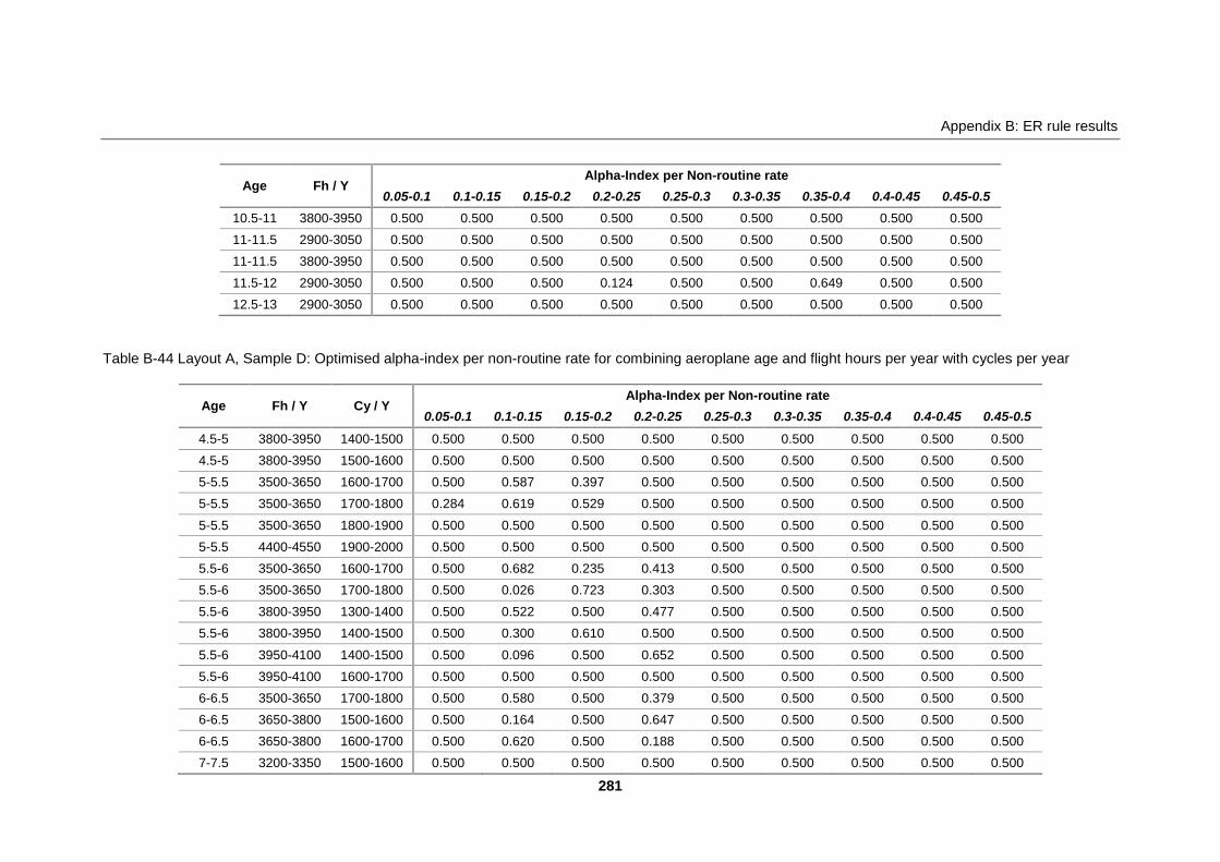
Appendix B: ER rule results
281
Age Fh / Y Alpha-Index per Non-routine rate
0.05-0.1 0.1-0.15 0.15-0.2 0.2-0.25 0.25-0.3 0.3-0.35 0.35-0.4 0.4-0.45 0.45-0.5
10.5-11 3800-3950 0.500 0.500 0.500 0.500 0.500 0.500 0.500 0.500 0.500
11-11.5 2900-3050 0.500 0.500 0.500 0.500 0.500 0.500 0.500 0.500 0.500
11-11.5 3800-3950 0.500 0.500 0.500 0.500 0.500 0.500 0.500 0.500 0.500
11.5-12 2900-3050 0.500 0.500 0.500 0.124 0.500 0.500 0.649 0.500 0.500
12.5-13 2900-3050 0.500 0.500 0.500 0.500 0.500 0.500 0.500 0.500 0.500
Table B-44 Layout A, Sample D: Optimised alpha-index per non-routine rate for combining aeroplane age and flight hours per year with cycles per year
Age Fh / Y Cy / Y Alpha-Index per Non-routine rate
0.05-0.1 0.1-0.15 0.15-0.2 0.2-0.25 0.25-0.3 0.3-0.35 0.35-0.4 0.4-0.45 0.45-0.5
4.5-5 3800-3950 1400-1500 0.500 0.500 0.500 0.500 0.500 0.500 0.500 0.500 0.500
4.5-5 3800-3950 1500-1600 0.500 0.500 0.500 0.500 0.500 0.500 0.500 0.500 0.500
5-5.5 3500-3650 1600-1700 0.500 0.587 0.397 0.500 0.500 0.500 0.500 0.500 0.500
5-5.5 3500-3650 1700-1800 0.284 0.619 0.529 0.500 0.500 0.500 0.500 0.500 0.500
5-5.5 3500-3650 1800-1900 0.500 0.500 0.500 0.500 0.500 0.500 0.500 0.500 0.500
5-5.5 4400-4550 1900-2000 0.500 0.500 0.500 0.500 0.500 0.500 0.500 0.500 0.500
5.5-6 3500-3650 1600-1700 0.500 0.682 0.235 0.413 0.500 0.500 0.500 0.500 0.500
5.5-6 3500-3650 1700-1800 0.500 0.026 0.723 0.303 0.500 0.500 0.500 0.500 0.500
5.5-6 3800-3950 1300-1400 0.500 0.522 0.500 0.477 0.500 0.500 0.500 0.500 0.500
5.5-6 3800-3950 1400-1500 0.500 0.300 0.610 0.500 0.500 0.500 0.500 0.500 0.500
5.5-6 3950-4100 1400-1500 0.500 0.096 0.500 0.652 0.500 0.500 0.500 0.500 0.500
5.5-6 3950-4100 1600-1700 0.500 0.500 0.500 0.500 0.500 0.500 0.500 0.500 0.500
6-6.5 3500-3650 1700-1800 0.500 0.580 0.500 0.379 0.500 0.500 0.500 0.500 0.500
6-6.5 3650-3800 1500-1600 0.500 0.164 0.500 0.647 0.500 0.500 0.500 0.500 0.500
6-6.5 3650-3800 1600-1700 0.500 0.620 0.500 0.188 0.500 0.500 0.500 0.500 0.500
7-7.5 3200-3350 1500-1600 0.500 0.500 0.500 0.500 0.500 0.500 0.500 0.500 0.500

Appendix B: ER rule results
282
Age Fh / Y Cy / Y Alpha-Index per Non-routine rate
0.05-0.1 0.1-0.15 0.15-0.2 0.2-0.25 0.25-0.3 0.3-0.35 0.35-0.4 0.4-0.45 0.45-0.5
7-7.5 3200-3350 1600-1700 0.500 0.500 0.500 0.500 0.500 0.500 0.500 0.500 0.500
7-7.5 3200-3350 1700-1800 0.500 0.500 0.500 0.500 0.500 0.500 0.500 0.500 0.500
7-7.5 3500-3650 1600-1700 0.500 0.500 0.500 0.500 0.500 0.500 0.500 0.500 0.500
7.5-8 3200-3350 1600-1700 0.500 0.500 0.500 0.500 0.436 0.197 0.672 0.500 0.500
7.5-8 3200-3350 1700-1800 0.500 0.500 0.500 0.567 0.337 0.500 0.503 0.500 0.500
7.5-8 3200-3350 1800-1900 0.500 0.500 0.500 0.500 0.452 0.500 0.543 0.500 0.500
7.5-8 3350-3500 1600-1700 0.500 0.500 0.500 0.500 0.500 0.500 0.500 0.500 0.500
7.5-8 3350-3500 1700-1800 0.500 0.500 0.500 0.420 0.571 0.500 0.500 0.500 0.500
7.5-8 3350-3500 1800-1900 0.500 0.500 0.500 0.500 0.500 0.500 0.500 0.500 0.500
7.5-8 3500-3650 1600-1700 0.500 0.500 0.128 0.648 0.533 0.461 0.500 0.500 0.500
7.5-8 3500-3650 1700-1800 0.500 0.500 0.500 0.239 0.651 0.500 0.500 0.500 0.500
7.5-8 3500-3650 1800-1900 0.500 0.500 0.500 0.500 0.500 0.500 0.500 0.500 0.500
8-8.5 3200-3350 1600-1700 0.500 0.500 0.500 0.500 0.500 0.500 0.500 0.500 0.500
9-9.5 2300-2450 900-1000 0.500 0.500 0.500 0.500 0.500 0.500 0.500 0.500 0.500
9-9.5 3200-3350 1600-1700 0.500 0.500 0.500 0.150 0.649 0.500 0.500 0.500 0.500
9-9.5 3200-3350 2000-2100 0.500 0.500 0.500 0.616 0.272 0.500 0.500 0.500 0.500
9-9.5 3350-3500 1600-1700 0.500 0.500 0.500 0.369 0.600 0.500 0.500 0.500 0.500
9-9.5 3350-3500 1700-1800 0.500 0.500 0.500 0.369 0.600 0.500 0.500 0.500 0.500
9.5-10 3200-3350 1600-1700 0.500 0.500 0.500 0.445 0.500 0.179 0.721 0.351 0.351
9.5-10 3200-3350 1700-1800 0.500 0.500 0.500 0.381 0.500 0.500 0.601 0.500 0.500
9.5-10 3200-3350 1900-2000 0.500 0.500 0.500 0.500 0.500 0.500 0.500 0.500 0.500
9.5-10 3350-3500 1200-1300 0.500 0.500 0.500 0.243 0.638 0.500 0.500 0.500 0.500
9.5-10 3350-3500 1600-1700 0.500 0.500 0.500 0.500 0.500 0.500 0.500 0.500 0.500
9.5-10 3500-3650 1200-1300 0.500 0.500 0.500 0.651 0.104 0.500 0.500 0.500 0.500
9.5-10 3650-3800 1200-1300 0.500 0.500 0.500 0.087 0.654 0.500 0.500 0.500 0.500
10-10.5 2900-3050 1400-1500 0.500 0.500 0.500 0.500 0.500 0.500 0.500 0.500 0.500

Appendix B: ER rule results
283
Age Fh / Y Cy / Y Alpha-Index per Non-routine rate
0.05-0.1 0.1-0.15 0.15-0.2 0.2-0.25 0.25-0.3 0.3-0.35 0.35-0.4 0.4-0.45 0.45-0.5
10-10.5 3500-3650 1900-2000 0.500 0.500 0.500 0.500 0.500 0.500 0.500 0.500 0.500
10.5-11 3200-3350 1700-1800 0.500 0.500 0.500 0.500 0.500 0.500 0.500 0.500 0.500
10.5-11 3800-3950 2600-2700 0.500 0.500 0.500 0.500 0.500 0.500 0.500 0.500 0.500
11-11.5 2900-3050 1400-1500 0.500 0.500 0.500 0.500 0.500 0.500 0.500 0.500 0.500
11-11.5 3800-3950 2600-2700 0.500 0.500 0.500 0.500 0.500 0.500 0.500 0.500 0.500
11.5-12 2900-3050 1300-1400 0.500 0.500 0.500 0.500 0.500 0.500 0.500 0.500 0.500
11.5-12 2900-3050 1400-1500 0.500 0.500 0.500 0.124 0.500 0.500 0.649 0.500 0.500
12.5-13 2900-3050 1000-1100 0.500 0.500 0.500 0.500 0.500 0.500 0.500 0.500 0.500
Table B-45 Layout A, Sample D: Optimised alpha-index per non-routine rate for combining aeroplane age, flight hours and cycles per year with service type
Age Fh / Y Cy / Y Service Alpha-Index per Non-routine rate
0.05-0.1 0.1-0.15 0.15-0.2 0.2-0.25 0.25-0.3 0.3-0.35 0.35-0.4 0.4-0.45 0.45-0.5
4.5-5 3800-3950 1400-1500 1C 0.500 0.500 0.500 0.500 0.500 0.500 0.500 0.500 0.500
4.5-5 3800-3950 1500-1600 1C 0.500 0.500 0.500 0.500 0.500 0.500 0.500 0.500 0.500
5-5.5 3500-3650 1600-1700 3C+ 0.500 0.587 0.397 0.500 0.500 0.500 0.500 0.500 0.500
5-5.5 3500-3650 1700-1800 3C 0.500 0.001 0.664 0.500 0.500 0.500 0.500 0.500 0.500
5-5.5 3500-3650 1700-1800 3C+ 0.284 0.713 0.174 0.500 0.500 0.500 0.500 0.500 0.500
5-5.5 3500-3650 1800-1900 3C+ 0.500 0.500 0.500 0.500 0.500 0.500 0.500 0.500 0.500
5-5.5 4400-4550 1900-2000 3C 0.500 0.500 0.500 0.500 0.500 0.500 0.500 0.500 0.500
5.5-6 3500-3650 1600-1700 3C+ 0.500 0.682 0.235 0.413 0.500 0.500 0.500 0.500 0.500
5.5-6 3500-3650 1700-1800 3C+ 0.500 0.026 0.723 0.303 0.500 0.500 0.500 0.500 0.500
5.5-6 3800-3950 1300-1400 3C+ 0.500 0.522 0.500 0.477 0.500 0.500 0.500 0.500 0.500
5.5-6 3800-3950 1400-1500 3C 0.500 0.300 0.610 0.500 0.500 0.500 0.500 0.500 0.500
5.5-6 3950-4100 1400-1500 2C 0.500 0.096 0.500 0.652 0.500 0.500 0.500 0.500 0.500
5.5-6 3950-4100 1600-1700 3C 0.500 0.500 0.500 0.500 0.500 0.500 0.500 0.500 0.500

Appendix B: ER rule results
284
Age Fh / Y Cy / Y Service Alpha-Index per Non-routine rate
0.05-0.1 0.1-0.15 0.15-0.2 0.2-0.25 0.25-0.3 0.3-0.35 0.35-0.4 0.4-0.45 0.45-0.5
6-6.5 3500-3650 1700-1800 2C 0.500 0.580 0.500 0.379 0.500 0.500 0.500 0.500 0.500
6-6.5 3650-3800 1500-1600 1C 0.500 0.500 0.500 0.500 0.500 0.500 0.500 0.500 0.500
6-6.5 3650-3800 1500-1600 2C 0.500 0.164 0.500 0.647 0.500 0.500 0.500 0.500 0.500
6-6.5 3650-3800 1600-1700 2C 0.500 0.620 0.500 0.188 0.500 0.500 0.500 0.500 0.500
7-7.5 3200-3350 1500-1600 1C 0.500 0.500 0.500 0.500 0.500 0.500 0.500 0.500 0.500
7-7.5 3200-3350 1600-1700 1C 0.500 0.500 0.500 0.500 0.500 0.500 0.500 0.500 0.500
7-7.5 3200-3350 1700-1800 1C 0.500 0.500 0.500 0.500 0.500 0.500 0.500 0.500 0.500
7-7.5 3500-3650 1600-1700 2C 0.500 0.500 0.500 0.500 0.500 0.500 0.500 0.500 0.500
7.5-8 3200-3350 1600-1700 4C 0.500 0.500 0.500 0.500 0.436 0.197 0.672 0.500 0.500
7.5-8 3200-3350 1700-1800 1C 0.500 0.500 0.500 0.500 0.500 0.500 0.500 0.500 0.500
7.5-8 3200-3350 1700-1800 4C 0.500 0.500 0.500 0.500 0.497 0.500 0.503 0.500 0.500
7.5-8 3200-3350 1700-1800 4C+ 0.500 0.500 0.500 0.567 0.342 0.500 0.500 0.500 0.500
7.5-8 3200-3350 1800-1900 4C 0.500 0.500 0.500 0.500 0.452 0.500 0.543 0.500 0.500
7.5-8 3350-3500 1600-1700 1C 0.500 0.500 0.500 0.500 0.500 0.500 0.500 0.500 0.500
7.5-8 3350-3500 1600-1700 4C 0.500 0.500 0.500 0.500 0.500 0.500 0.500 0.500 0.500
7.5-8 3350-3500 1700-1800 4C+ 0.500 0.500 0.500 0.420 0.571 0.500 0.500 0.500 0.500
7.5-8 3350-3500 1800-1900 4C+ 0.500 0.500 0.500 0.500 0.500 0.500 0.500 0.500 0.500
7.5-8 3500-3650 1600-1700 3C+ 0.500 0.500 0.128 0.648 0.500 0.500 0.500 0.500 0.500
7.5-8 3500-3650 1600-1700 4C 0.500 0.500 0.500 0.500 0.533 0.461 0.500 0.500 0.500
7.5-8 3500-3650 1700-1800 4C+ 0.500 0.500 0.500 0.239 0.651 0.500 0.500 0.500 0.500
7.5-8 3500-3650 1800-1900 4C+ 0.500 0.500 0.500 0.500 0.500 0.500 0.500 0.500 0.500
8-8.5 3200-3350 1600-1700 4C 0.500 0.500 0.500 0.500 0.500 0.500 0.500 0.500 0.500
9-9.5 2300-2450 900-1000 2C 0.500 0.500 0.500 0.500 0.500 0.500 0.500 0.500 0.500
9-9.5 3200-3350 1600-1700 2C 0.500 0.500 0.500 0.150 0.649 0.500 0.500 0.500 0.500
9-9.5 3200-3350 2000-2100 5C+ 0.500 0.500 0.500 0.616 0.272 0.500 0.500 0.500 0.500
9-9.5 3350-3500 1600-1700 2C 0.500 0.500 0.500 0.369 0.600 0.500 0.500 0.500 0.500

Appendix B: ER rule results
285
Age Fh / Y Cy / Y Service Alpha-Index per Non-routine rate
0.05-0.1 0.1-0.15 0.15-0.2 0.2-0.25 0.25-0.3 0.3-0.35 0.35-0.4 0.4-0.45 0.45-0.5
9-9.5 3350-3500 1700-1800 2C 0.500 0.500 0.500 0.369 0.600 0.500 0.500 0.500 0.500
9.5-10 3200-3350 1600-1700 5C 0.500 0.500 0.500 0.445 0.500 0.179 0.721 0.351 0.351
9.5-10 3200-3350 1700-1800 5C 0.500 0.500 0.500 0.381 0.500 0.500 0.601 0.500 0.500
9.5-10 3200-3350 1900-2000 5C 0.500 0.500 0.500 0.500 0.500 0.500 0.500 0.500 0.500
9.5-10 3350-3500 1200-1300 5C+ 0.500 0.500 0.500 0.243 0.638 0.500 0.500 0.500 0.500
9.5-10 3350-3500 1600-1700 5C 0.500 0.500 0.500 0.500 0.500 0.500 0.500 0.500 0.500
9.5-10 3500-3650 1200-1300 5C+ 0.500 0.500 0.500 0.651 0.104 0.500 0.500 0.500 0.500
9.5-10 3650-3800 1200-1300 5C+ 0.500 0.500 0.500 0.087 0.654 0.500 0.500 0.500 0.500
10-10.5 2900-3050 1400-1500 3C+ 0.500 0.500 0.500 0.500 0.500 0.500 0.500 0.500 0.500
10-10.5 3500-3650 1900-2000 3C+ 0.500 0.500 0.500 0.500 0.500 0.500 0.500 0.500 0.500
10.5-11 3200-3350 1700-1800 1C 0.500 0.500 0.500 0.500 0.500 0.500 0.500 0.500 0.500
10.5-11 3200-3350 1700-1800 3C+ 0.500 0.500 0.500 0.500 0.500 0.500 0.500 0.500 0.500
10.5-11 3800-3950 2600-2700 3C 0.500 0.500 0.500 0.500 0.500 0.500 0.500 0.500 0.500
11-11.5 2900-3050 1400-1500 1C 0.500 0.500 0.500 0.500 0.500 0.500 0.500 0.500 0.500
11-11.5 3800-3950 2600-2700 6C 0.500 0.500 0.500 0.500 0.500 0.500 0.500 0.500 0.500
11.5-12 2900-3050 1300-1400 6C 0.500 0.500 0.500 0.500 0.500 0.500 0.500 0.500 0.500
11.5-12 2900-3050 1400-1500 6C 0.500 0.500 0.500 0.124 0.500 0.500 0.649 0.500 0.500
12.5-13 2900-3050 1000-1100 2C 0.500 0.500 0.500 0.500 0.500 0.500 0.500 0.500 0.500

Appendix B: ER rule results
286
Table B-46 Layout B, Sample A: Optimised alpha-index per non-routine rate for combining
aeroplane age and flight hours per year
Age Fh / Y Alpha-Index per Non-routine rate
0-0.1 0.1-0.2 0.2-0.3 0.3-0.4 0.4-0.5
2.5-5 3800-3950 0.500 0.500 0.500 0.500 0.500
5-7.5 3200-3350 0.500 0.500 0.500 0.500 0.500
5-7.5 3500-3650 0.386 0.597 0.462 0.500 0.500
5-7.5 3650-3800 0.500 0.480 0.518 0.500 0.500
5-7.5 3800-3950 0.500 0.524 0.476 0.500 0.500
5-7.5 3950-4100 0.500 0.500 0.500 0.500 0.500
5-7.5 4400-4550 0.500 0.500 0.500 0.500 0.500
7.5-10 2300-2450 0.500 0.500 0.500 0.500 0.500
7.5-10 3200-3350 0.500 0.166 0.335 0.746 0.595
7.5-10 3350-3500 0.500 0.490 0.510 0.500 0.500
7.5-10 3500-3650 0.500 0.094 0.644 0.440 0.500
7.5-10 3650-3800 0.500 0.500 0.500 0.500 0.500
10-12.5 2900-3050 0.500 0.500 0.283 0.590 0.500
10-12.5 3200-3350 0.500 0.679 0.201 0.500 0.500
10-12.5 3800-3950 0.500 0.500 0.500 0.500 0.500
12.5-15 2900-3050 0.500 0.500 0.500 0.500 0.500
Table B-47 Layout B, Sample A: Optimised alpha-index per non-routine rate for combining
aeroplane age and flight hours per year with cycles per year
Age Fh / Y Cy / Y Alpha-Index per Non-routine rate
0-0.1 0.1-0.2 0.2-0.3 0.3-0.4 0.4-0.5
2.5-5 3800-3950 1200-1500 0.500 0.500 0.500 0.500 0.500
2.5-5 3800-3950 1500-1800 0.500 0.500 0.500 0.500 0.500
5-7.5 3200-3350 1500-1800 0.500 0.500 0.500 0.500 0.500
5-7.5 3500-3650 1500-1800 0.386 0.597 0.462 0.500 0.500
5-7.5 3650-3800 1500-1800 0.500 0.480 0.518 0.500 0.500
5-7.5 3800-3950 1200-1500 0.500 0.524 0.476 0.500 0.500
5-7.5 3950-4100 1500-1800 0.500 0.500 0.500 0.500 0.500
5-7.5 4400-4550 1800-2100 0.500 0.500 0.500 0.500 0.500
7.5-10 2300-2450 900-1200 0.500 0.500 0.500 0.500 0.500
7.5-10 3200-3350 1500-1800 0.500 0.166 0.512 0.613 0.595
7.5-10 3200-3350 1800-2100 0.500 0.500 0.281 0.663 0.500
7.5-10 3350-3500 1200-1500 0.500 0.500 0.500 0.500 0.500
7.5-10 3350-3500 1500-1800 0.500 0.490 0.510 0.500 0.500
7.5-10 3350-3500 1800-2100 0.500 0.500 0.500 0.500 0.500

Appendix B: ER rule results
287
Age Fh / Y Cy / Y Alpha-Index per Non-routine rate
0-0.1 0.1-0.2 0.2-0.3 0.3-0.4 0.4-0.5
7.5-10 3500-3650 1200-1500 0.500 0.500 0.500 0.500 0.500
7.5-10 3500-3650 1500-1800 0.500 0.094 0.644 0.440 0.500
7.5-10 3500-3650 1800-2100 0.500 0.500 0.500 0.500 0.500
7.5-10 3650-3800 1200-1500 0.500 0.500 0.500 0.500 0.500
10-12.5 2900-3050 1200-1500 0.500 0.500 0.283 0.590 0.500
10-12.5 3200-3350 1500-1800 0.500 0.582 0.405 0.500 0.500
10-12.5 3200-3350 1800-2100 0.500 0.622 0.327 0.500 0.500
10-12.5 3800-3950 2400-2700 0.500 0.500 0.500 0.500 0.500
12.5-15 2900-3050 900-1200 0.500 0.500 0.500 0.500 0.500
Table B-48 Layout B, Sample A: Optimised alpha-index per non-routine rate for combining
aeroplane age, flight hours and cycles per year with service type
Age Fh / Y Cy / Y Service Alpha-Index per Non-routine rate
0-0.1 0.1-0.2 0.2-0.3 0.3-0.4 0.4-0.5
2.5-5 3800-3950 1200-1500 1C 0.500 0.500 0.500 0.500 0.500
2.5-5 3800-3950 1500-1800 1C 0.500 0.500 0.500 0.500 0.500
5-7.5 3200-3350 1500-1800 1C 0.500 0.500 0.500 0.500 0.500
5-7.5 3500-3650 1500-1800 2C 0.500 0.273 0.640 0.500 0.500
5-7.5 3500-3650 1500-1800 3C 0.500 0.500 0.500 0.500 0.500
5-7.5 3500-3650 1500-1800 3C+ 0.386 0.706 0.260 0.500 0.500
5-7.5 3650-3800 1500-1800 1C 0.500 0.500 0.500 0.500 0.500
5-7.5 3650-3800 1500-1800 2C 0.500 0.480 0.518 0.500 0.500
5-7.5 3650-3800 1500-1800 3C 0.500 0.500 0.500 0.500 0.500
5-7.5 3800-3950 1200-1500 3C 0.500 0.500 0.500 0.500 0.500
5-7.5 3800-3950 1200-1500 3C+ 0.500 0.524 0.476 0.500 0.500
5-7.5 3950-4100 1500-1800 3C 0.500 0.500 0.500 0.500 0.500
5-7.5 3950-4100 1500-1800 3C+ 0.500 0.500 0.500 0.500 0.500
5-7.5 4400-4550 1800-2100 3C 0.500 0.500 0.500 0.500 0.500
7.5-10 2300-2450 900-1200 2C 0.500 0.500 0.500 0.500 0.500
7.5-10 3200-3350 1500-1800 1C 0.500 0.500 0.500 0.500 0.500
7.5-10 3200-3350 1500-1800 2C 0.500 0.166 0.671 0.500 0.500
7.5-10 3200-3350 1500-1800 4C 0.500 0.500 0.357 0.621 0.500
7.5-10 3200-3350 1500-1800 4C+ 0.500 0.500 0.500 0.500 0.500
7.5-10 3200-3350 1500-1800 5C 0.500 0.500 0.405 0.490 0.595
7.5-10 3200-3350 1800-2100 4C 0.500 0.500 0.436 0.558 0.500
7.5-10 3200-3350 1800-2100 5C 0.500 0.500 0.357 0.617 0.500
7.5-10 3200-3350 1800-2100 5C+ 0.500 0.500 0.500 0.500 0.500

Appendix B: ER rule results
288
Age Fh / Y Cy / Y Service Alpha-Index per Non-routine rate
0-0.1 0.1-0.2 0.2-0.3 0.3-0.4 0.4-0.5
7.5-10 3350-3500 1200-1500 5C+ 0.500 0.500 0.500 0.500 0.500
7.5-10 3350-3500 1500-1800 1C 0.500 0.500 0.500 0.500 0.500
7.5-10 3350-3500 1500-1800 2C 0.500 0.490 0.510 0.500 0.500
7.5-10 3350-3500 1500-1800 4C 0.500 0.500 0.500 0.500 0.500
7.5-10 3350-3500 1500-1800 4C+ 0.500 0.500 0.500 0.500 0.500
7.5-10 3350-3500 1500-1800 5C 0.500 0.500 0.500 0.500 0.500
7.5-10 3350-3500 1800-2100 4C+ 0.500 0.500 0.500 0.500 0.500
7.5-10 3500-3650 1200-1500 5C+ 0.500 0.500 0.500 0.500 0.500
7.5-10 3500-3650 1500-1800 3C+ 0.500 0.094 0.619 0.500 0.500
7.5-10 3500-3650 1500-1800 4C 0.500 0.500 0.548 0.440 0.500
7.5-10 3500-3650 1500-1800 4C+ 0.500 0.500 0.500 0.500 0.500
7.5-10 3500-3650 1800-2100 4C+ 0.500 0.500 0.500 0.500 0.500
7.5-10 3650-3800 1200-1500 5C+ 0.500 0.500 0.500 0.500 0.500
10-12.5 2900-3050 1200-1500 1C 0.500 0.500 0.500 0.500 0.500
10-12.5 2900-3050 1200-1500 6C 0.500 0.500 0.283 0.590 0.500
10-12.5 3200-3350 1500-1800 1C 0.500 0.500 0.500 0.500 0.500
10-12.5 3200-3350 1500-1800 3C+ 0.500 0.582 0.405 0.500 0.500
10-12.5 3200-3350 1800-2100 3C+ 0.500 0.622 0.327 0.500 0.500
10-12.5 3800-3950 2400-2700 3C 0.500 0.500 0.500 0.500 0.500
10-12.5 3800-3950 2400-2700 6C 0.500 0.500 0.500 0.500 0.500
12.5-15 2900-3050 900-1200 2C 0.500 0.500 0.500 0.500 0.500

Appendix B: ER rule results
289
Table B-49 Layout B, Sample B: Optimised alpha-index per non-routine rate for combining
aeroplane age and flight hours per year
Age Fh / Y Alpha-Index per Non-routine rate
0-0.1 0.1-0.2 0.2-0.3 0.3-0.4 0.4-0.5
2.5-5 3800-3950 0.498 0.498 0.498 0.498 0.498
5-7.5 3200-3350 0.498 0.498 0.498 0.498 0.498
5-7.5 3500-3650 0.412 0.636 0.392 0.498 0.498
5-7.5 3650-3800 0.498 0.498 0.498 0.498 0.498
5-7.5 3800-3950 0.498 0.503 0.493 0.498 0.498
5-7.5 3950-4100 0.498 0.378 0.493 0.498 0.498
5-7.5 4400-4550 0.498 0.498 0.498 0.498 0.498
7.5-10 2300-2450 0.498 0.498 0.498 0.498 0.498
7.5-10 3200-3350 0.498 0.244 0.221 0.757 0.627
7.5-10 3350-3500 0.498 0.498 0.498 0.498 0.498
7.5-10 3500-3650 0.498 0.092 0.589 0.498 0.498
7.5-10 3650-3800 0.498 0.498 0.498 0.498 0.498
10-12.5 2900-3050 0.498 0.647 0.283 0.498 0.498
10-12.5 3200-3350 0.498 0.705 0.201 0.498 0.498
10-12.5 3500-3650 0.498 0.650 0.285 0.498 0.498
10-12.5 3800-3950 0.498 0.498 0.498 0.498 0.498
12.5-15 2900-3050 0.498 0.498 0.498 0.498 0.498
Table B-50 Layout B, Sample B: Optimised alpha-index per non-routine rate for combining
aeroplane age and flight hours per year with cycles per year
Age Fh / Y Cy / Y Alpha-Index per Non-routine rate
0-0.1 0.1-0.2 0.2-0.3 0.3-0.4 0.4-0.5
2.5-5 3800-3950 1200-1500 0.498 0.498 0.498 0.498 0.498
2.5-5 3800-3950 1500-1800 0.498 0.498 0.498 0.498 0.498
5-7.5 3200-3350 1500-1800 0.498 0.498 0.498 0.498 0.498
5-7.5 3500-3650 1500-1800 0.412 0.501 0.543 0.498 0.498
5-7.5 3500-3650 1800-2100 0.498 0.643 0.323 0.498 0.498
5-7.5 3650-3800 1500-1800 0.498 0.498 0.498 0.498 0.498
5-7.5 3800-3950 1200-1500 0.498 0.503 0.493 0.498 0.498
5-7.5 3950-4100 1200-1500 0.498 0.036 0.593 0.498 0.498
5-7.5 3950-4100 1500-1800 0.498 0.638 0.327 0.498 0.498
5-7.5 4400-4550 1800-2100 0.498 0.498 0.498 0.498 0.498
7.5-10 2300-2450 900-1200 0.498 0.498 0.498 0.498 0.498
7.5-10 3200-3350 1500-1800 0.498 0.244 0.482 0.602 0.627
7.5-10 3200-3350 1800-2100 0.498 0.498 0.249 0.674 0.498
7.5-10 3350-3500 1200-1500 0.498 0.498 0.498 0.498 0.498
7.5-10 3350-3500 1500-1800 0.498 0.498 0.498 0.498 0.498
7.5-10 3350-3500 1800-2100 0.498 0.498 0.498 0.498 0.498
7.5-10 3500-3650 1200-1500 0.498 0.498 0.498 0.498 0.498
7.5-10 3500-3650 1500-1800 0.498 0.092 0.589 0.498 0.498

Appendix B: ER rule results
290
Age Fh / Y Cy / Y Alpha-Index per Non-routine rate
0-0.1 0.1-0.2 0.2-0.3 0.3-0.4 0.4-0.5
7.5-10 3500-3650 1800-2100 0.498 0.498 0.498 0.498 0.498
7.5-10 3650-3800 1200-1500 0.498 0.498 0.498 0.498 0.498
10-12.5 2900-3050 1200-1500 0.498 0.647 0.283 0.498 0.498
10-12.5 3200-3350 1500-1800 0.498 0.604 0.374 0.498 0.498
10-12.5 3200-3350 1800-2100 0.498 0.618 0.353 0.498 0.498
10-12.5 3500-3650 1800-2100 0.498 0.650 0.285 0.498 0.498
10-12.5 3800-3950 2400-2700 0.498 0.498 0.498 0.498 0.498
12.5-15 2900-3050 900-1200 0.498 0.498 0.498 0.498 0.498
Table B-51 Layout B, Sample B: Optimised alpha-index per non-routine rate for combining
aeroplane age, flight hours and cycles per year with service type
Age Fh / Y Cy / Y Service Alpha-Index per Non-routine rate
0-0.1 0.1-0.2 0.2-0.3 0.3-0.4 0.4-0.5
2.5-5 3800-3950 1200-1500 1C 0.498 0.498 0.498 0.498 0.498
2.5-5 3800-3950 1500-1800 1C 0.498 0.498 0.498 0.498 0.498
5-7.5 3200-3350 1500-1800 1C 0.498 0.498 0.498 0.498 0.498
5-7.5 3500-3650 1500-1800 2C 0.498 0.312 0.623 0.498 0.498
5-7.5 3500-3650 1500-1800 3C 0.498 0.498 0.498 0.498 0.498
5-7.5 3500-3650 1500-1800 3C+ 0.412 0.615 0.399 0.498 0.498
5-7.5 3500-3650 1800-2100 3C+ 0.498 0.643 0.323 0.498 0.498
5-7.5 3650-3800 1500-1800 1C 0.498 0.498 0.498 0.498 0.498
5-7.5 3650-3800 1500-1800 2C 0.498 0.498 0.498 0.498 0.498
5-7.5 3650-3800 1500-1800 3C 0.498 0.498 0.498 0.498 0.498
5-7.5 3800-3950 1200-1500 3C 0.498 0.498 0.498 0.498 0.498
5-7.5 3800-3950 1200-1500 3C+ 0.498 0.503 0.493 0.498 0.498
5-7.5 3950-4100 1200-1500 2C 0.498 0.036 0.593 0.498 0.498
5-7.5 3950-4100 1500-1800 3C 0.498 0.498 0.498 0.498 0.498
5-7.5 3950-4100 1500-1800 3C+ 0.498 0.638 0.327 0.498 0.498
5-7.5 4400-4550 1800-2100 3C 0.498 0.498 0.498 0.498 0.498
7.5-10 2300-2450 900-1200 2C 0.498 0.498 0.498 0.498 0.498
7.5-10 3200-3350 1500-1800 1C 0.498 0.498 0.498 0.498 0.498
7.5-10 3200-3350 1500-1800 2C 0.498 0.244 0.702 0.498 0.498
7.5-10 3200-3350 1500-1800 4C 0.498 0.498 0.319 0.644 0.498
7.5-10 3200-3350 1500-1800 4C+ 0.498 0.498 0.498 0.498 0.498
7.5-10 3200-3350 1500-1800 5C 0.498 0.498 0.402 0.441 0.627
7.5-10 3200-3350 1800-2100 4C 0.498 0.498 0.409 0.577 0.498
7.5-10 3200-3350 1800-2100 5C 0.498 0.498 0.360 0.611 0.498
7.5-10 3200-3350 1800-2100 5C+ 0.498 0.498 0.498 0.498 0.498
7.5-10 3350-3500 1200-1500 5C+ 0.498 0.498 0.498 0.498 0.498
7.5-10 3350-3500 1500-1800 2C 0.498 0.498 0.498 0.498 0.498
7.5-10 3350-3500 1500-1800 4C 0.498 0.498 0.498 0.498 0.498
7.5-10 3350-3500 1500-1800 4C+ 0.498 0.498 0.498 0.498 0.498
7.5-10 3350-3500 1500-1800 5C 0.498 0.498 0.498 0.498 0.498

Appendix B: ER rule results
291
Age Fh / Y Cy / Y Service Alpha-Index per Non-routine rate
0-0.1 0.1-0.2 0.2-0.3 0.3-0.4 0.4-0.5
7.5-10 3350-3500 1800-2100 4C+ 0.498 0.498 0.498 0.498 0.498
7.5-10 3500-3650 1200-1500 5C+ 0.498 0.498 0.498 0.498 0.498
7.5-10 3500-3650 1500-1800 3C+ 0.498 0.092 0.589 0.498 0.498
7.5-10 3500-3650 1500-1800 4C 0.498 0.498 0.498 0.498 0.498
7.5-10 3500-3650 1500-1800 4C+ 0.498 0.498 0.498 0.498 0.498
7.5-10 3500-3650 1800-2100 4C+ 0.498 0.498 0.498 0.498 0.498
7.5-10 3650-3800 1200-1500 5C+ 0.498 0.498 0.498 0.498 0.498
10-12.5 2900-3050 1200-1500 1C 0.498 0.498 0.498 0.498 0.498
10-12.5 2900-3050 1200-1500 3C+ 0.498 0.647 0.283 0.498 0.498
10-12.5 2900-3050 1200-1500 6C 0.498 0.498 0.498 0.498 0.498
10-12.5 3200-3350 1500-1800 1C 0.498 0.498 0.498 0.498 0.498
10-12.5 3200-3350 1500-1800 3C+ 0.498 0.604 0.374 0.498 0.498
10-12.5 3200-3350 1800-2100 3C+ 0.498 0.618 0.353 0.498 0.498
10-12.5 3500-3650 1800-2100 3C+ 0.498 0.650 0.285 0.498 0.498
10-12.5 3800-3950 2400-2700 6C 0.498 0.498 0.498 0.498 0.498
12.5-15 2900-3050 900-1200 2C 0.498 0.498 0.498 0.498 0.498

Appendix B: ER rule results
292
Table B-52 Layout B, Sample C: Optimised alpha-index per non-routine rate for combining
aeroplane age and flight hours per year
Age Fh / Y Alpha-Index per Non-routine rate
0-0.1 0.1-0.2 0.2-0.3 0.3-0.4 0.4-0.5
2.5-5 3800-3950 0.500 0.500 0.500 0.500 0.500
5-7.5 3200-3350 0.500 0.500 0.500 0.500 0.500
5-7.5 3500-3650 0.405 0.637 0.387 0.500 0.500
5-7.5 3650-3800 0.500 0.203 0.645 0.500 0.500
5-7.5 3800-3950 0.500 0.500 0.500 0.500 0.500
5-7.5 3950-4100 0.500 0.408 0.561 0.500 0.500
5-7.5 4400-4550 0.500 0.500 0.500 0.500 0.500
7.5-10 2300-2450 0.500 0.500 0.500 0.500 0.500
7.5-10 3200-3350 0.500 0.240 0.148 0.728 0.596
7.5-10 3350-3500 0.500 0.499 0.502 0.500 0.500
7.5-10 3500-3650 0.500 0.071 0.675 0.402 0.500
7.5-10 3650-3800 0.500 0.500 0.500 0.500 0.500
10-12.5 2900-3050 0.500 0.647 0.285 0.484 0.500
10-12.5 3200-3350 0.500 0.683 0.205 0.500 0.500
10-12.5 3500-3650 0.500 0.621 0.354 0.500 0.500
10-12.5 3800-3950 0.500 0.500 0.500 0.500 0.500
12.5-15 2900-3050 0.500 0.500 0.500 0.500 0.500
Table B-53 Layout B, Sample C: Optimised alpha-index per non-routine rate for combining
aeroplane age and flight hours per year with cycles per year
Age Fh / Y Cy / Y Alpha-Index per Non-routine rate
0-0.1 0.1-0.2 0.2-0.3 0.3-0.4 0.4-0.5
2.5-5 3800-3950 1200-1500 0.500 0.500 0.500 0.500 0.500
2.5-5 3800-3950 1500-1800 0.500 0.500 0.500 0.500 0.500
5-7.5 3200-3350 1500-1800 0.500 0.500 0.500 0.500 0.500
5-7.5 3500-3650 1500-1800 0.405 0.560 0.497 0.500 0.500
5-7.5 3500-3650 1800-2100 0.500 0.594 0.395 0.500 0.500
5-7.5 3650-3800 1500-1800 0.500 0.203 0.645 0.500 0.500
5-7.5 3800-3950 1200-1500 0.500 0.500 0.500 0.500 0.500
5-7.5 3950-4100 1200-1500 0.500 0.066 0.652 0.500 0.500
5-7.5 3950-4100 1500-1800 0.500 0.638 0.318 0.500 0.500
5-7.5 4400-4550 1800-2100 0.500 0.500 0.500 0.500 0.500
7.5-10 2300-2450 900-1200 0.500 0.500 0.500 0.500 0.500
7.5-10 3200-3350 1500-1800 0.500 0.240 0.457 0.641 0.596
7.5-10 3200-3350 1800-2100 0.500 0.500 0.228 0.644 0.500
7.5-10 3350-3500 1200-1500 0.500 0.500 0.500 0.500 0.500
7.5-10 3350-3500 1500-1800 0.500 0.499 0.502 0.500 0.500
7.5-10 3350-3500 1800-2100 0.500 0.500 0.500 0.500 0.500
7.5-10 3500-3650 1500-1800 0.500 0.071 0.675 0.402 0.500
7.5-10 3500-3650 1800-2100 0.500 0.500 0.500 0.500 0.500

Appendix B: ER rule results
293
Age Fh / Y Cy / Y Alpha-Index per Non-routine rate
0-0.1 0.1-0.2 0.2-0.3 0.3-0.4 0.4-0.5
7.5-10 3650-3800 1200-1500 0.500 0.500 0.500 0.500 0.500
10-12.5 2900-3050 1200-1500 0.500 0.647 0.285 0.484 0.500
10-12.5 3200-3350 1500-1800 0.500 0.597 0.383 0.500 0.500
10-12.5 3200-3350 1800-2100 0.500 0.611 0.356 0.500 0.500
10-12.5 3500-3650 1800-2100 0.500 0.621 0.354 0.500 0.500
10-12.5 3800-3950 2400-2700 0.500 0.500 0.500 0.500 0.500
12.5-15 2900-3050 900-1200 0.500 0.500 0.500 0.500 0.500
Table B-54 Layout B, Sample C: Optimised alpha-index per non-routine rate for combining
aeroplane age, flight hours and cycles per year with service type
Age Fh / Y Cy / Y Service Alpha-Index per Non-routine rate
0-0.1 0.1-0.2 0.2-0.3 0.3-0.4 0.4-0.5
2.5-5 3800-3950 1200-1500 1C 0.500 0.500 0.500 0.500 0.500
2.5-5 3800-3950 1500-1800 1C 0.500 0.500 0.500 0.500 0.500
5-7.5 3200-3350 1500-1800 1C 0.500 0.500 0.500 0.500 0.500
5-7.5 3500-3650 1500-1800 2C 0.500 0.475 0.525 0.500 0.500
5-7.5 3500-3650 1500-1800 3C 0.500 0.500 0.500 0.500 0.500
5-7.5 3500-3650 1500-1800 3C+ 0.405 0.586 0.472 0.500 0.500
5-7.5 3500-3650 1800-2100 3C+ 0.500 0.594 0.395 0.500 0.500
5-7.5 3650-3800 1500-1800 1C 0.500 0.500 0.500 0.500 0.500
5-7.5 3650-3800 1500-1800 2C 0.500 0.203 0.645 0.500 0.500
5-7.5 3650-3800 1500-1800 3C 0.500 0.500 0.500 0.500 0.500
5-7.5 3800-3950 1200-1500 3C 0.500 0.500 0.500 0.500 0.500
5-7.5 3800-3950 1200-1500 3C+ 0.500 0.500 0.500 0.500 0.500
5-7.5 3950-4100 1200-1500 2C 0.500 0.066 0.652 0.500 0.500
5-7.5 3950-4100 1500-1800 3C 0.500 0.500 0.500 0.500 0.500
5-7.5 3950-4100 1500-1800 3C+ 0.500 0.638 0.318 0.500 0.500
5-7.5 4400-4550 1800-2100 3C 0.500 0.500 0.500 0.500 0.500
7.5-10 2300-2450 900-1200 2C 0.500 0.500 0.500 0.500 0.500
7.5-10 3200-3350 1500-1800 1C 0.500 0.500 0.500 0.500 0.500
7.5-10 3200-3350 1500-1800 2C 0.500 0.240 0.692 0.500 0.500
7.5-10 3200-3350 1500-1800 4C 0.500 0.500 0.317 0.635 0.500
7.5-10 3200-3350 1500-1800 4C+ 0.500 0.500 0.500 0.500 0.500
7.5-10 3200-3350 1500-1800 5C 0.500 0.500 0.382 0.504 0.596
7.5-10 3200-3350 1800-2100 4C 0.500 0.500 0.412 0.571 0.500
7.5-10 3200-3350 1800-2100 5C 0.500 0.500 0.354 0.599 0.500
7.5-10 3200-3350 1800-2100 5C+ 0.500 0.500 0.500 0.500 0.500
7.5-10 3350-3500 1200-1500 5C+ 0.500 0.500 0.500 0.500 0.500
7.5-10 3350-3500 1500-1800 1C 0.500 0.500 0.500 0.500 0.500
7.5-10 3350-3500 1500-1800 2C 0.500 0.499 0.502 0.500 0.500
7.5-10 3350-3500 1500-1800 4C 0.500 0.500 0.500 0.500 0.500
7.5-10 3350-3500 1500-1800 4C+ 0.500 0.500 0.500 0.500 0.500
7.5-10 3350-3500 1500-1800 5C 0.500 0.500 0.500 0.500 0.500

Appendix B: ER rule results
294
Age Fh / Y Cy / Y Service Alpha-Index per Non-routine rate
0-0.1 0.1-0.2 0.2-0.3 0.3-0.4 0.4-0.5
7.5-10 3350-3500 1800-2100 4C+ 0.500 0.500 0.500 0.500 0.500
7.5-10 3500-3650 1500-1800 3C+ 0.500 0.071 0.638 0.500 0.500
7.5-10 3500-3650 1500-1800 4C 0.500 0.500 0.566 0.402 0.500
7.5-10 3500-3650 1800-2100 4C+ 0.500 0.500 0.500 0.500 0.500
7.5-10 3650-3800 1200-1500 5C+ 0.500 0.500 0.500 0.500 0.500
10-12.5 2900-3050 1200-1500 1C 0.500 0.500 0.500 0.500 0.500
10-12.5 2900-3050 1200-1500 3C+ 0.500 0.647 0.294 0.500 0.500
10-12.5 2900-3050 1200-1500 6C 0.500 0.500 0.515 0.484 0.500
10-12.5 3200-3350 1500-1800 1C 0.500 0.500 0.500 0.500 0.500
10-12.5 3200-3350 1500-1800 3C+ 0.500 0.597 0.383 0.500 0.500
10-12.5 3200-3350 1800-2100 3C+ 0.500 0.611 0.356 0.500 0.500
10-12.5 3500-3650 1800-2100 3C+ 0.500 0.621 0.354 0.500 0.500
10-12.5 3800-3950 2400-2700 3C 0.500 0.500 0.500 0.500 0.500
12.5-15 2900-3050 900-1200 2C 0.500 0.500 0.500 0.500 0.500

Appendix B: ER rule results
295
Table B-55 Layout B, Sample D: Optimised alpha-index per non-routine rate for combining
aeroplane age and flight hours per year
Age Fh / Y Alpha-Index per Non-routine rate
0-0.1 0.1-0.2 0.2-0.3 0.3-0.4 0.4-0.5
2.5-5 3800-3950 0.498 0.498 0.498 0.498 0.498
5-7.5 3200-3350 0.498 0.498 0.498 0.498 0.498
5-7.5 3500-3650 0.400 0.665 0.377 0.498 0.498
5-7.5 3650-3800 0.498 0.526 0.471 0.498 0.498
5-7.5 3800-3950 0.498 0.503 0.494 0.498 0.498
5-7.5 3950-4100 0.498 0.111 0.637 0.498 0.498
5-7.5 4400-4550 0.498 0.498 0.498 0.498 0.498
7.5-10 2300-2450 0.498 0.498 0.498 0.498 0.498
7.5-10 3200-3350 0.498 0.260 0.207 0.744 0.596
7.5-10 3350-3500 0.498 0.495 0.501 0.498 0.498
7.5-10 3500-3650 0.498 0.098 0.650 0.452 0.498
7.5-10 3650-3800 0.498 0.498 0.498 0.498 0.498
10-12.5 2900-3050 0.498 0.605 0.323 0.525 0.498
10-12.5 3200-3350 0.498 0.632 0.326 0.498 0.498
10-12.5 3500-3650 0.498 0.637 0.313 0.498 0.498
10-12.5 3800-3950 0.498 0.498 0.498 0.498 0.498
12.5-15 2900-3050 0.498 0.498 0.498 0.498 0.498
Table B-56 Layout B, Sample D: Optimised alpha-index per non-routine rate for combining
aeroplane age and flight hours per year with cycles per year
Age Fh / Y Cy / Y Alpha-Index per Non-routine rate
0-0.1 0.1-0.2 0.2-0.3 0.3-0.4 0.4-0.5
2.5-5 3800-3950 1200-1500 0.498 0.498 0.498 0.498 0.498
2.5-5 3800-3950 1500-1800 0.498 0.498 0.498 0.498 0.498
5-7.5 3200-3350 1500-1800 0.498 0.498 0.498 0.498 0.498
5-7.5 3500-3650 1500-1800 0.400 0.536 0.544 0.498 0.498
5-7.5 3500-3650 1800-2100 0.498 0.648 0.298 0.498 0.498
5-7.5 3650-3800 1500-1800 0.498 0.526 0.471 0.498 0.498
5-7.5 3800-3950 1200-1500 0.498 0.503 0.494 0.498 0.498
5-7.5 3950-4100 1200-1500 0.498 0.111 0.637 0.498 0.498
5-7.5 3950-4100 1500-1800 0.498 0.498 0.498 0.498 0.498
5-7.5 4400-4550 1800-2100 0.498 0.498 0.498 0.498 0.498
7.5-10 2300-2450 900-1200 0.498 0.498 0.498 0.498 0.498
7.5-10 3200-3350 1500-1800 0.498 0.260 0.452 0.635 0.596
7.5-10 3200-3350 1800-2100 0.498 0.498 0.260 0.660 0.498
7.5-10 3350-3500 1200-1500 0.498 0.498 0.498 0.498 0.498
7.5-10 3350-3500 1500-1800 0.498 0.495 0.501 0.498 0.498
7.5-10 3350-3500 1800-2100 0.498 0.498 0.498 0.498 0.498
7.5-10 3500-3650 1200-1500 0.498 0.498 0.498 0.498 0.498
7.5-10 3500-3650 1500-1800 0.498 0.098 0.650 0.452 0.498

Appendix B: ER rule results
296
Age Fh / Y Cy / Y Alpha-Index per Non-routine rate
0-0.1 0.1-0.2 0.2-0.3 0.3-0.4 0.4-0.5
7.5-10 3500-3650 1800-2100 0.498 0.498 0.498 0.498 0.498
7.5-10 3650-3800 1200-1500 0.498 0.498 0.498 0.498 0.498
10-12.5 2900-3050 1200-1500 0.498 0.605 0.323 0.525 0.498
10-12.5 3200-3350 1500-1800 0.498 0.632 0.326 0.498 0.498
10-12.5 3500-3650 1800-2100 0.498 0.637 0.313 0.498 0.498
10-12.5 3800-3950 2400-2700 0.498 0.498 0.498 0.498 0.498
12.5-15 2900-3050 900-1200 0.498 0.498 0.498 0.498 0.498
Table B-57 Layout B, Sample D: Optimised alpha-index per non-routine rate for combining
aeroplane age, flight hours and cycles per year with service type
Age Fh / Y Cy / Y Service Alpha-Index per Non-routine rate
0-0.1 0.1-0.2 0.2-0.3 0.3-0.4 0.4-0.5
2.5-5 3800-3950 1200-1500 1C 0.498 0.498 0.498 0.498 0.498
2.5-5 3800-3950 1500-1800 1C 0.498 0.498 0.498 0.498 0.498
5-7.5 3200-3350 1500-1800 1C 0.498 0.498 0.498 0.498 0.498
5-7.5 3500-3650 1500-1800 2C 0.498 0.298 0.638 0.498 0.498
5-7.5 3500-3650 1500-1800 3C 0.498 0.498 0.498 0.498 0.498
5-7.5 3500-3650 1500-1800 3C+ 0.400 0.657 0.375 0.498 0.498
5-7.5 3500-3650 1800-2100 3C+ 0.498 0.648 0.298 0.498 0.498
5-7.5 3650-3800 1500-1800 1C 0.498 0.498 0.498 0.498 0.498
5-7.5 3650-3800 1500-1800 2C 0.498 0.526 0.471 0.498 0.498
5-7.5 3800-3950 1200-1500 3C 0.498 0.498 0.498 0.498 0.498
5-7.5 3800-3950 1200-1500 3C+ 0.498 0.503 0.494 0.498 0.498
5-7.5 3950-4100 1200-1500 2C 0.498 0.111 0.637 0.498 0.498
5-7.5 3950-4100 1500-1800 3C 0.498 0.498 0.498 0.498 0.498
5-7.5 4400-4550 1800-2100 3C 0.498 0.498 0.498 0.498 0.498
7.5-10 2300-2450 900-1200 2C 0.498 0.498 0.498 0.498 0.498
7.5-10 3200-3350 1500-1800 1C 0.498 0.498 0.498 0.498 0.498
7.5-10 3200-3350 1500-1800 2C 0.498 0.260 0.677 0.498 0.498
7.5-10 3200-3350 1500-1800 4C 0.498 0.498 0.322 0.636 0.498
7.5-10 3200-3350 1500-1800 4C+ 0.498 0.498 0.498 0.498 0.498
7.5-10 3200-3350 1500-1800 5C 0.498 0.498 0.388 0.496 0.596
7.5-10 3200-3350 1800-2100 4C 0.498 0.498 0.416 0.570 0.498
7.5-10 3200-3350 1800-2100 5C 0.498 0.498 0.355 0.611 0.498
7.5-10 3200-3350 1800-2100 5C+ 0.498 0.498 0.498 0.498 0.498
7.5-10 3350-3500 1200-1500 5C+ 0.498 0.498 0.498 0.498 0.498
7.5-10 3350-3500 1500-1800 1C 0.498 0.498 0.498 0.498 0.498
7.5-10 3350-3500 1500-1800 2C 0.498 0.495 0.501 0.498 0.498
7.5-10 3350-3500 1500-1800 4C 0.498 0.498 0.498 0.498 0.498
7.5-10 3350-3500 1500-1800 4C+ 0.498 0.498 0.498 0.498 0.498
7.5-10 3350-3500 1500-1800 5C 0.498 0.498 0.498 0.498 0.498
7.5-10 3350-3500 1800-2100 4C+ 0.498 0.498 0.498 0.498 0.498
7.5-10 3500-3650 1200-1500 5C+ 0.498 0.498 0.498 0.498 0.498

Appendix B: ER rule results
297
Age Fh / Y Cy / Y Service Alpha-Index per Non-routine rate
0-0.1 0.1-0.2 0.2-0.3 0.3-0.4 0.4-0.5
7.5-10 3500-3650 1500-1800 3C+ 0.498 0.098 0.628 0.498 0.498
7.5-10 3500-3650 1500-1800 4C 0.498 0.498 0.547 0.452 0.498
7.5-10 3500-3650 1500-1800 4C+ 0.498 0.498 0.498 0.498 0.498
7.5-10 3500-3650 1800-2100 4C+ 0.498 0.498 0.498 0.498 0.498
7.5-10 3650-3800 1200-1500 5C+ 0.498 0.498 0.498 0.498 0.498
10-12.5 2900-3050 1200-1500 1C 0.498 0.498 0.498 0.498 0.498
10-12.5 2900-3050 1200-1500 3C+ 0.498 0.605 0.375 0.498 0.498
10-12.5 2900-3050 1200-1500 6C 0.498 0.498 0.470 0.525 0.498
10-12.5 3200-3350 1500-1800 1C 0.498 0.498 0.498 0.498 0.498
10-12.5 3200-3350 1500-1800 3C+ 0.498 0.632 0.326 0.498 0.498
10-12.5 3500-3650 1800-2100 3C+ 0.498 0.637 0.313 0.498 0.498
10-12.5 3800-3950 2400-2700 3C 0.498 0.498 0.498 0.498 0.498
10-12.5 3800-3950 2400-2700 6C 0.498 0.498 0.498 0.498 0.498
12.5-15 2900-3050 900-1200 2C 0.498 0.498 0.498 0.498 0.498

Appendix B: ER rule results
298
B.7.2 Optimised weights results
Table B-58 Layout A (Four samples): Optimised weights for each piece of evidence
Variable No. Interval Interval Sample A Sample B Sample C Sample D
Age
1 4.5 - 5 0.660 0.852 0.813 0.854
2 5 - 5.5 0.384 0.238 0.312 0.402
3 5.5 - 6 0.662 0.809 0.204 0.667
4 6 - 6.5 0.293 0.313 0.032 0.051
5 6.5 - 7 0.500 0.504 0.500 0.502
6 7 - 7.5 0.568 0.019 0.053 0.096
7 7.5 - 8 0.353 0.328 0.481 0.449
8 8 - 8.5 0.424 0.477 0.263 0.343
9 8.5 - 9 0.500 0.504 0.500 0.502
10 9 - 9.5 0.347 0.103 0.315 0.372
11 9.5 - 10 0.164 0.024 0.023 0.023
12 10 - 10.5 0.500 0.868 0.816 0.912
13 10.5 - 11 0.652 0.541 0.405 0.346
14 11 - 11.5 0.555 0.680 0.594 0.641
15 11.5 - 12 0.524 0.504 0.307 0.758
16 12 - 12.5 0.500 0.504 0.500 0.502
17 12.5 - 13 0.444 0.479 0.330 0.355
Fh/Y
1 2300 - 2450 0.523 0.559 0.602 0.598
2 2450 - 2600 0.500 0.504 0.500 0.502
3 2600 - 2750 0.500 0.504 0.500 0.502
4 2750 - 2900 0.500 0.504 0.500 0.502
5 2900 - 3050 0.408 0.201 0.020 0.067
6 3050 - 3200 0.500 0.504 0.500 0.502
7 3200 - 3350 0.068 0.004 0.006 0.011
8 3350 - 3500 0.732 0.914 0.860 0.871
9 3500 - 3650 0.454 0.013 0.416 0.246
10 3650 - 3800 0.281 0.306 0.109 0.046
11 3800 - 3950 0.521 0.771 0.842 0.741
12 3950 - 4100 0.519 0.705 0.058 0.671
13 4100 - 4250 0.500 0.504 0.500 0.502
14 4250 - 4400 0.500 0.504 0.500 0.502
15 4400 - 4550 0.594 0.679 0.648 0.715
Cy/Y
1 900 - 1000 0.523 0.559 0.602 0.598
2 1000 - 1100 0.440 0.476 0.315 0.338
3 1100 - 1200 0.500 0.504 0.500 0.502
4 1200 - 1300 0.501 0.426 0.496 0.419
5 1300 - 1400 0.696 0.695 0.762 0.905
6 1400 - 1500 0.667 0.723 0.021 0.306
7 1500 - 1600 0.555 0.303 0.716 0.650

Appendix B: ER rule results
299
Variable No. Interval Interval Sample A Sample B Sample C Sample D
8 1600 - 1700 0.070 0.049 0.010 0.022
9 1700 - 1800 0.055 0.015 0.014 0.011
10 1800 - 1900 0.582 0.071 0.040 0.034
11 1900 - 2000 0.603 0.173 0.130 0.219
12 2000 - 2100 0.578 0.504 0.500 0.502
13 2100 - 2200 0.500 0.504 0.500 0.502
14 2200 - 2300 0.500 0.504 0.500 0.502
15 2300 - 2400 0.500 0.504 0.500 0.502
16 2400 - 2500 0.500 0.504 0.500 0.502
17 2500 - 2600 0.500 0.504 0.500 0.502
18 2600 - 2700 0.515 0.633 0.207 0.623
Services
1 1C 0.843 0.835 0.908 0.868
2 2C 0.613 0.157 0.434 0.264
3 3C 0.649 0.646 0.802 0.871
4 3C+ 0.230 0.128 0.051 0.044
5 4C 0.541 0.711 0.513 0.315
6 4C+ 0.676 0.834 0.868 0.866
7 5C 0.089 0.030 0.025 0.022
8 5C+ 0.532 0.431 0.485 0.644
9 6C+ 0.645 0.641 0.195 0.818
Nr rate 1 0.037 0.003 0.002 0.002
Figure B-30 Layout A: Optimised weights for each piece of evidence
0.00
0.20
0.40
0.60
0.80
1.00
1 3 5 7 9 11131517 2 4 6 8 101214 1 3 5 7 9 11131517 1 3 5 7 9
Age Fh/Y Cy/Y ServicesNr rate
We
igh
t
Optimised Weight of each Piece of Evidence
Sample A Sample B Sample C Sample D
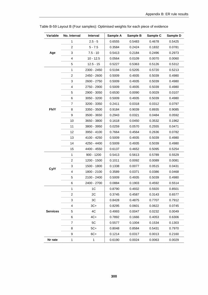
Appendix B: ER rule results
300
Table B-59 Layout B (Four samples): Optimised weights for each piece of evidence
Variable No. Interval Interval Sample A Sample B Sample C Sample D
Age
1 2.5 - 5 0.6555 0.5483 0.4678 0.5425
2 5 - 7.5 0.3584 0.2424 0.1832 0.0781
3 7.5 - 10 0.5413 0.2184 0.2496 0.2973
4 10 - 12.5 0.0564 0.0109 0.0070 0.0060
5 12.5 - 15 0.5227 0.5363 0.5126 0.5312
Fh/Y
1 2300 - 2450 0.5194 0.5205 0.5720 0.5213
2 2450 - 2600 0.5009 0.4935 0.5039 0.4980
3 2600 - 2750 0.5009 0.4935 0.5039 0.4980
4 2750 - 2900 0.5009 0.4935 0.5039 0.4980
5 2900 - 3050 0.6530 0.0090 0.0029 0.0107
6 3050 - 3200 0.5009 0.4935 0.5039 0.4980
7 3200 - 3350 0.2411 0.0318 0.0312 0.0797
8 3350 - 3500 0.9184 0.9039 0.8935 0.9085
9 3500 - 3650 0.2943 0.0321 0.0484 0.0592
10 3650 - 3800 0.1618 0.0450 0.3532 0.1962
11 3800 - 3950 0.0259 0.0570 0.2555 0.0471
12 3950 - 4100 0.7664 0.4564 0.2636 0.0782
13 4100 - 4250 0.5009 0.4935 0.5039 0.4980
14 4250 - 4400 0.5009 0.4935 0.5039 0.4980
15 4400 - 4550 0.6137 0.4652 0.5095 0.5254
Cy/Y
1 900 - 1200 0.5413 0.5613 0.5789 0.5529
2 1200 - 1500 0.1011 0.0092 0.0089 0.0081
3 1500 - 1800 0.1338 0.0077 0.0515 0.0431
4 1800 - 2100 0.3589 0.0371 0.0386 0.0468
5 2100 - 2400 0.5009 0.4935 0.5039 0.4980
6 2400 - 2700 0.0884 0.1903 0.4592 0.5514
Services
1 1C 0.8790 0.4932 0.5920 0.8501
2 2C 0.3745 0.4587 0.3143 0.6577
3 3C 0.8428 0.4875 0.7707 0.7912
4 3C+ 0.8295 0.0601 0.0622 0.0745
5 4C 0.4993 0.0047 0.0232 0.0049
6 4C+ 0.7892 0.1666 0.4053 0.6306
7 5C 0.5577 0.1004 0.1534 0.1303
8 5C+ 0.8048 0.8584 0.5431 0.7970
9 6C+ 0.1214 0.0317 0.0013 0.2160
Nr rate 1 1 0.6190 0.0024 0.0063 0.0029

Appendix B: ER rule results
301
Figure B-31 Layout B: Optimised weights for each piece of evidence
0.00
0.20
0.40
0.60
0.80
1.00
1 3 5 2 4 6 8 10 12 14 1 3 5 1 3 5 7 9
Age Fh/Y Cy/Y Services Nr rate
We
igh
t
Optimised Weight of each Piece of Evidence
Sample A Sample B Sample C Sample D

Appendix B: ER rule results
302
B.8 Sensitivity analysis results
B.8.1 Sensitivity analysis when the reliability of one variable is modified at a time
Table B-60 Layout A, Sample A: Sensibility analysis when alpha index has been optimised, weight is one and the reliability of one variable is modified at a time
Reliability 0 0.05 0.1 0.15 0.2 0.25 0.3 0.35 0.4 0.45 0.5 0.55 0.6 0.65 0.7 0.75 0.8 0.85 0.9 0.95 1
Age
MSESERV 0.001 0.001 0.001 0.001 0.001 0.001 0.001 0.001 0.001 0.001 0.001 0.001 0.001 0.001 0.001 0.001 0.001 0.001 0.001 0.001 0.000
MAE 0.017 0.017 0.017 0.017 0.017 0.017 0.017 0.017 0.017 0.017 0.017 0.017 0.017 0.017 0.017 0.017 0.017 0.016 0.016 0.016 0.016
MPAE 9.4% 9.4% 9.4% 9.4% 9.4% 9.4% 9.3% 9.3% 9.3% 9.3% 9.2% 9.2% 9.2% 9.1% 9.0% 9.0% 8.9% 8.7% 8.6% 8.5% 8.0%
MAI 95.9% 95.9% 95.9% 95.9% 95.9% 95.9% 95.9% 95.9% 96.0% 96.0% 96.0% 96.0% 96.0% 96.0% 96.1% 96.1% 96.1% 96.1% 96.2% 96.2% 96.3%
Fh/y
MSESERV 0.001 0.001 0.001 0.001 0.001 0.001 0.001 0.001 0.001 0.001 0.001 0.001 0.001 0.001 0.001 0.001 0.001 0.001 0.001 0.001 0.000
MAE 0.021 0.021 0.021 0.021 0.020 0.020 0.020 0.020 0.020 0.020 0.020 0.020 0.020 0.020 0.020 0.020 0.020 0.020 0.020 0.019 0.016
MPAE 9.9% 9.9% 9.9% 9.9% 9.9% 9.9% 9.9% 9.9% 9.9% 9.9% 9.9% 9.9% 9.9% 9.8% 9.8% 9.8% 9.8% 9.8% 9.7% 9.5% 8.0%
MAI 95.2% 95.2% 95.2% 95.2% 95.2% 95.2% 95.2% 95.2% 95.2% 95.2% 95.2% 95.2% 95.2% 95.2% 95.2% 95.2% 95.3% 95.3% 95.3% 95.4% 96.3%
Cy/y
MSESERV 0.001 0.001 0.001 0.001 0.001 0.001 0.001 0.001 0.001 0.001 0.001 0.001 0.001 0.001 0.001 0.001 0.001 0.001 0.001 0.001 0.000
MAE 0.019 0.019 0.019 0.019 0.019 0.019 0.019 0.019 0.018 0.018 0.018 0.018 0.018 0.018 0.018 0.018 0.018 0.018 0.018 0.017 0.016
MPAE 9.1% 9.1% 9.1% 9.1% 9.1% 9.1% 9.1% 9.1% 9.1% 9.0% 9.0% 9.0% 9.0% 9.0% 8.9% 8.9% 8.8% 8.8% 8.7% 8.6% 8.0%
MAI 95.6% 95.6% 95.6% 95.6% 95.6% 95.6% 95.6% 95.6% 95.7% 95.7% 95.7% 95.7% 95.7% 95.7% 95.7% 95.7% 95.8% 95.8% 95.8% 95.9% 96.3%
Services
MSESERV 0.001 0.001 0.001 0.001 0.001 0.001 0.001 0.001 0.001 0.001 0.001 0.001 0.001 0.001 0.001 0.001 0.001 0.001 0.001 0.001 0.000
MAE 0.024 0.024 0.024 0.024 0.024 0.024 0.024 0.024 0.023 0.023 0.023 0.023 0.023 0.023 0.022 0.022 0.022 0.021 0.020 0.019 0.016
MPAE 11.9% 11.9% 11.9% 11.9% 11.9% 11.8% 11.8% 11.8% 11.7% 11.7% 11.6% 11.6% 11.5% 11.4% 11.3% 11.1% 11.0% 10.7% 10.4% 9.8% 8.0%
MAI 94.4% 94.4% 94.4% 94.4% 94.4% 94.4% 94.4% 94.5% 94.5% 94.5% 94.5% 94.6% 94.6% 94.7% 94.7% 94.8% 94.9% 95.1% 95.2% 95.5% 96.3%
NRR
MSESERV 0.000 0.000 0.000 0.000 0.000 0.000 0.000 0.000 0.000 0.000 0.000 0.000 0.000 0.000 0.000 0.000 0.000 0.000 0.000 0.000 0.000
MAE 0.017 0.017 0.017 0.017 0.017 0.017 0.017 0.017 0.017 0.017 0.017 0.017 0.017 0.017 0.017 0.017 0.017 0.017 0.016 0.016 0.016
MPAE 8.9% 8.9% 8.9% 8.9% 8.9% 8.9% 8.8% 8.8% 8.8% 8.8% 8.8% 8.8% 8.8% 8.8% 8.8% 8.7% 8.7% 8.6% 8.6% 8.4% 8.0%
MAI 96.0% 96.0% 96.0% 96.0% 96.0% 96.0% 96.0% 96.0% 96.0% 96.0% 96.0% 96.0% 96.0% 96.0% 96.0% 96.0% 96.1% 96.1% 96.1% 96.2% 96.3%
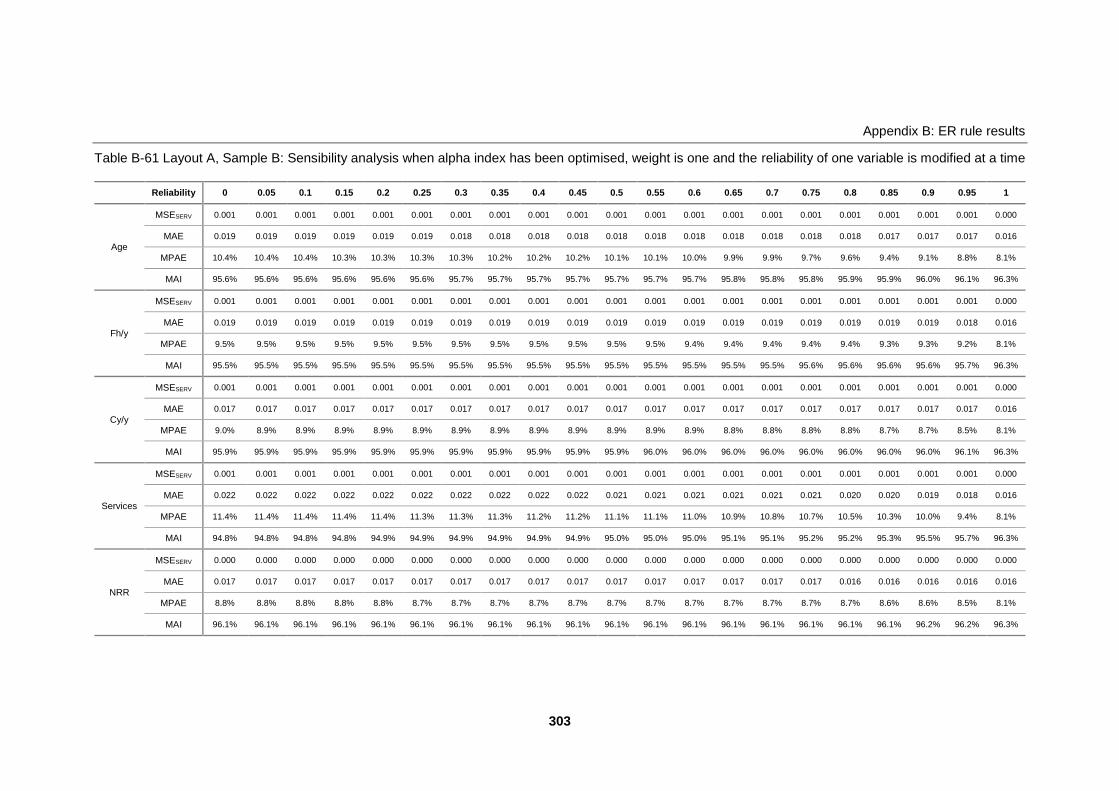
Appendix B: ER rule results
303
Table B-61 Layout A, Sample B: Sensibility analysis when alpha index has been optimised, weight is one and the reliability of one variable is modified at a time
Reliability 0 0.05 0.1 0.15 0.2 0.25 0.3 0.35 0.4 0.45 0.5 0.55 0.6 0.65 0.7 0.75 0.8 0.85 0.9 0.95 1
Age
MSESERV 0.001 0.001 0.001 0.001 0.001 0.001 0.001 0.001 0.001 0.001 0.001 0.001 0.001 0.001 0.001 0.001 0.001 0.001 0.001 0.001 0.000
MAE 0.019 0.019 0.019 0.019 0.019 0.019 0.018 0.018 0.018 0.018 0.018 0.018 0.018 0.018 0.018 0.018 0.018 0.017 0.017 0.017 0.016
MPAE 10.4% 10.4% 10.4% 10.3% 10.3% 10.3% 10.3% 10.2% 10.2% 10.2% 10.1% 10.1% 10.0% 9.9% 9.9% 9.7% 9.6% 9.4% 9.1% 8.8% 8.1%
MAI 95.6% 95.6% 95.6% 95.6% 95.6% 95.6% 95.7% 95.7% 95.7% 95.7% 95.7% 95.7% 95.7% 95.8% 95.8% 95.8% 95.9% 95.9% 96.0% 96.1% 96.3%
Fh/y
MSESERV 0.001 0.001 0.001 0.001 0.001 0.001 0.001 0.001 0.001 0.001 0.001 0.001 0.001 0.001 0.001 0.001 0.001 0.001 0.001 0.001 0.000
MAE 0.019 0.019 0.019 0.019 0.019 0.019 0.019 0.019 0.019 0.019 0.019 0.019 0.019 0.019 0.019 0.019 0.019 0.019 0.019 0.018 0.016
MPAE 9.5% 9.5% 9.5% 9.5% 9.5% 9.5% 9.5% 9.5% 9.5% 9.5% 9.5% 9.5% 9.4% 9.4% 9.4% 9.4% 9.4% 9.3% 9.3% 9.2% 8.1%
MAI 95.5% 95.5% 95.5% 95.5% 95.5% 95.5% 95.5% 95.5% 95.5% 95.5% 95.5% 95.5% 95.5% 95.5% 95.5% 95.6% 95.6% 95.6% 95.6% 95.7% 96.3%
Cy/y
MSESERV 0.001 0.001 0.001 0.001 0.001 0.001 0.001 0.001 0.001 0.001 0.001 0.001 0.001 0.001 0.001 0.001 0.001 0.001 0.001 0.001 0.000
MAE 0.017 0.017 0.017 0.017 0.017 0.017 0.017 0.017 0.017 0.017 0.017 0.017 0.017 0.017 0.017 0.017 0.017 0.017 0.017 0.017 0.016
MPAE 9.0% 8.9% 8.9% 8.9% 8.9% 8.9% 8.9% 8.9% 8.9% 8.9% 8.9% 8.9% 8.9% 8.8% 8.8% 8.8% 8.8% 8.7% 8.7% 8.5% 8.1%
MAI 95.9% 95.9% 95.9% 95.9% 95.9% 95.9% 95.9% 95.9% 95.9% 95.9% 95.9% 96.0% 96.0% 96.0% 96.0% 96.0% 96.0% 96.0% 96.0% 96.1% 96.3%
Services
MSESERV 0.001 0.001 0.001 0.001 0.001 0.001 0.001 0.001 0.001 0.001 0.001 0.001 0.001 0.001 0.001 0.001 0.001 0.001 0.001 0.001 0.000
MAE 0.022 0.022 0.022 0.022 0.022 0.022 0.022 0.022 0.022 0.022 0.021 0.021 0.021 0.021 0.021 0.021 0.020 0.020 0.019 0.018 0.016
MPAE 11.4% 11.4% 11.4% 11.4% 11.4% 11.3% 11.3% 11.3% 11.2% 11.2% 11.1% 11.1% 11.0% 10.9% 10.8% 10.7% 10.5% 10.3% 10.0% 9.4% 8.1%
MAI 94.8% 94.8% 94.8% 94.8% 94.9% 94.9% 94.9% 94.9% 94.9% 94.9% 95.0% 95.0% 95.0% 95.1% 95.1% 95.2% 95.2% 95.3% 95.5% 95.7% 96.3%
NRR
MSESERV 0.000 0.000 0.000 0.000 0.000 0.000 0.000 0.000 0.000 0.000 0.000 0.000 0.000 0.000 0.000 0.000 0.000 0.000 0.000 0.000 0.000
MAE 0.017 0.017 0.017 0.017 0.017 0.017 0.017 0.017 0.017 0.017 0.017 0.017 0.017 0.017 0.017 0.017 0.016 0.016 0.016 0.016 0.016
MPAE 8.8% 8.8% 8.8% 8.8% 8.8% 8.7% 8.7% 8.7% 8.7% 8.7% 8.7% 8.7% 8.7% 8.7% 8.7% 8.7% 8.7% 8.6% 8.6% 8.5% 8.1%
MAI 96.1% 96.1% 96.1% 96.1% 96.1% 96.1% 96.1% 96.1% 96.1% 96.1% 96.1% 96.1% 96.1% 96.1% 96.1% 96.1% 96.1% 96.1% 96.2% 96.2% 96.3%

Appendix B: ER rule results
304
Table B-62 Layout A, Sample C: Sensibility analysis when alpha index has been optimised, weight is one and the reliability of one variable is modified at a time
Reliability 0 0.05 0.1 0.15 0.2 0.25 0.3 0.35 0.4 0.45 0.5 0.55 0.6 0.65 0.7 0.75 0.8 0.85 0.9 0.95 1
Age
MSESERV 0.001 0.001 0.001 0.001 0.001 0.001 0.001 0.001 0.001 0.001 0.001 0.001 0.001 0.000 0.000 0.000 0.000 0.000 0.000 0.000 0.000
MAE 0.017 0.017 0.017 0.017 0.017 0.017 0.017 0.017 0.016 0.016 0.016 0.016 0.016 0.016 0.016 0.016 0.016 0.016 0.016 0.016 0.015
MPAE 8.9% 8.9% 8.9% 8.9% 8.9% 8.8% 8.8% 8.8% 8.8% 8.7% 8.7% 8.7% 8.6% 8.6% 8.5% 8.4% 8.4% 8.3% 8.2% 8.0% 7.5%
MAI 96.1% 96.1% 96.1% 96.1% 96.1% 96.1% 96.1% 96.1% 96.1% 96.1% 96.1% 96.2% 96.2% 96.2% 96.2% 96.2% 96.3% 96.3% 96.3% 96.3% 96.6%
Fh/y
MSESERV 0.001 0.001 0.001 0.001 0.001 0.001 0.001 0.001 0.001 0.001 0.001 0.001 0.001 0.001 0.001 0.001 0.001 0.001 0.001 0.001 0.000
MAE 0.019 0.019 0.019 0.019 0.019 0.019 0.019 0.019 0.019 0.019 0.019 0.019 0.019 0.019 0.019 0.019 0.019 0.019 0.018 0.018 0.015
MPAE 9.4% 9.4% 9.4% 9.4% 9.4% 9.4% 9.4% 9.3% 9.3% 9.3% 9.3% 9.3% 9.3% 9.3% 9.3% 9.2% 9.2% 9.2% 9.1% 8.9% 7.5%
MAI 95.5% 95.5% 95.5% 95.5% 95.5% 95.5% 95.5% 95.5% 95.5% 95.5% 95.5% 95.5% 95.5% 95.5% 95.5% 95.6% 95.6% 95.6% 95.7% 95.8% 96.6%
Cy/y
MSESERV 0.001 0.001 0.001 0.001 0.001 0.001 0.001 0.001 0.001 0.001 0.001 0.001 0.001 0.001 0.001 0.001 0.001 0.001 0.001 0.000 0.000
MAE 0.018 0.018 0.018 0.018 0.017 0.017 0.017 0.017 0.017 0.017 0.017 0.017 0.017 0.017 0.017 0.017 0.017 0.017 0.016 0.016 0.015
MPAE 8.5% 8.5% 8.5% 8.5% 8.5% 8.5% 8.5% 8.4% 8.4% 8.4% 8.4% 8.4% 8.4% 8.3% 8.3% 8.3% 8.2% 8.1% 8.0% 7.8% 7.5%
MAI 95.9% 95.9% 95.9% 95.9% 95.9% 95.9% 95.9% 95.9% 95.9% 95.9% 95.9% 95.9% 96.0% 96.0% 96.0% 96.0% 96.0% 96.1% 96.1% 96.3% 96.6%
Services
MSESERV 0.001 0.001 0.001 0.001 0.001 0.001 0.001 0.001 0.001 0.001 0.001 0.001 0.001 0.001 0.001 0.001 0.001 0.001 0.001 0.001 0.000
MAE 0.024 0.024 0.023 0.023 0.023 0.023 0.023 0.023 0.023 0.023 0.023 0.022 0.022 0.022 0.022 0.021 0.021 0.020 0.019 0.018 0.015
MPAE 11.7% 11.7% 11.7% 11.7% 11.6% 11.6% 11.6% 11.5% 11.5% 11.4% 11.3% 11.3% 11.2% 11.1% 11.0% 10.8% 10.6% 10.3% 9.8% 9.0% 7.5%
MAI 94.5% 94.5% 94.5% 94.5% 94.5% 94.5% 94.6% 94.6% 94.6% 94.6% 94.7% 94.7% 94.8% 94.8% 94.9% 95.0% 95.1% 95.2% 95.5% 95.8% 96.6%
NRR
MSESERV 0.000 0.000 0.000 0.000 0.000 0.000 0.000 0.000 0.000 0.000 0.000 0.000 0.000 0.000 0.000 0.000 0.000 0.000 0.000 0.000 0.000
MAE 0.016 0.016 0.016 0.016 0.016 0.016 0.016 0.016 0.016 0.016 0.016 0.016 0.016 0.016 0.016 0.016 0.016 0.016 0.015 0.015 0.015
MPAE 8.3% 8.3% 8.3% 8.3% 8.3% 8.3% 8.3% 8.3% 8.3% 8.3% 8.3% 8.3% 8.3% 8.3% 8.3% 8.2% 8.2% 8.2% 8.1% 8.0% 7.5%
MAI 96.3% 96.3% 96.3% 96.3% 96.3% 96.3% 96.3% 96.3% 96.3% 96.3% 96.3% 96.3% 96.3% 96.3% 96.3% 96.3% 96.3% 96.3% 96.4% 96.4% 96.6%

Appendix B: ER rule results
305
Table B-63 Layout A, Sample D: Sensibility analysis when alpha index has been optimised, weight is one and the reliability of one variable is modified at a time
Reliability 0 0.05 0.1 0.15 0.2 0.25 0.3 0.35 0.4 0.45 0.5 0.55 0.6 0.65 0.7 0.75 0.8 0.85 0.9 0.95 1
Age
MSESERV 0.001 0.001 0.001 0.001 0.001 0.001 0.001 0.001 0.001 0.001 0.001 0.001 0.001 0.001 0.001 0.001 0.001 0.001 0.001 0.001 0.000
MAE 0.017 0.017 0.017 0.017 0.017 0.017 0.017 0.017 0.017 0.017 0.017 0.017 0.017 0.017 0.017 0.017 0.016 0.016 0.016 0.016 0.015
MPAE 9.7% 9.7% 9.7% 9.7% 9.7% 9.7% 9.6% 9.6% 9.6% 9.6% 9.5% 9.5% 9.4% 9.4% 9.3% 9.2% 9.0% 8.9% 8.7% 8.4% 8.1%
MAI 95.9% 95.9% 95.9% 95.9% 95.9% 96.0% 96.0% 96.0% 96.0% 96.0% 96.0% 96.0% 96.0% 96.0% 96.1% 96.1% 96.1% 96.2% 96.2% 96.3% 96.4%
Fh/y
MSESERV 0.001 0.001 0.001 0.001 0.001 0.001 0.001 0.001 0.001 0.001 0.001 0.001 0.001 0.001 0.001 0.001 0.001 0.001 0.001 0.001 0.000
MAE 0.020 0.020 0.020 0.020 0.020 0.020 0.020 0.020 0.019 0.019 0.019 0.019 0.019 0.019 0.019 0.019 0.019 0.019 0.019 0.019 0.015
MPAE 9.6% 9.6% 9.6% 9.6% 9.6% 9.6% 9.6% 9.6% 9.6% 9.6% 9.6% 9.6% 9.6% 9.6% 9.5% 9.5% 9.5% 9.5% 9.4% 9.3% 8.1%
MAI 95.4% 95.4% 95.4% 95.4% 95.4% 95.4% 95.4% 95.4% 95.4% 95.4% 95.4% 95.4% 95.4% 95.4% 95.4% 95.5% 95.5% 95.5% 95.5% 95.6% 96.4%
Cy/y
MSESERV 0.001 0.001 0.001 0.001 0.001 0.001 0.001 0.001 0.001 0.001 0.001 0.001 0.001 0.001 0.001 0.001 0.001 0.001 0.001 0.001 0.000
MAE 0.018 0.018 0.018 0.018 0.018 0.018 0.018 0.018 0.018 0.018 0.018 0.018 0.018 0.018 0.018 0.018 0.018 0.018 0.018 0.017 0.015
MPAE 9.3% 9.2% 9.2% 9.2% 9.2% 9.2% 9.2% 9.2% 9.2% 9.2% 9.2% 9.2% 9.1% 9.1% 9.1% 9.1% 9.0% 8.9% 8.8% 8.6% 8.1%
MAI 95.7% 95.7% 95.7% 95.7% 95.7% 95.7% 95.7% 95.7% 95.7% 95.7% 95.7% 95.7% 95.7% 95.8% 95.8% 95.8% 95.8% 95.8% 95.9% 96.0% 96.4%
Services
MSESERV 0.001 0.001 0.001 0.001 0.001 0.001 0.001 0.001 0.001 0.001 0.001 0.001 0.001 0.001 0.001 0.001 0.001 0.001 0.001 0.001 0.000
MAE 0.023 0.023 0.023 0.023 0.023 0.023 0.023 0.023 0.023 0.023 0.023 0.023 0.023 0.022 0.022 0.022 0.022 0.021 0.021 0.020 0.015
MPAE 12.1% 12.1% 12.0% 12.0% 12.0% 12.0% 12.0% 11.9% 11.9% 11.9% 11.8% 11.8% 11.7% 11.6% 11.5% 11.4% 11.3% 11.1% 10.8% 10.3% 8.1%
MAI 94.5% 94.5% 94.5% 94.5% 94.5% 94.5% 94.5% 94.6% 94.6% 94.6% 94.6% 94.6% 94.7% 94.7% 94.8% 94.8% 94.9% 95.0% 95.1% 95.4% 96.4%
NRR
MSESERV 0.000 0.000 0.000 0.000 0.000 0.000 0.000 0.000 0.000 0.000 0.000 0.000 0.000 0.000 0.000 0.000 0.000 0.000 0.000 0.000 0.000
MAE 0.017 0.017 0.017 0.017 0.017 0.017 0.017 0.017 0.017 0.017 0.017 0.017 0.017 0.017 0.017 0.017 0.017 0.017 0.016 0.016 0.015
MPAE 9.0% 9.0% 8.9% 8.9% 8.9% 8.9% 8.9% 8.9% 8.9% 8.9% 8.9% 8.9% 8.9% 8.9% 8.9% 8.8% 8.8% 8.7% 8.6% 8.4% 8.1%
MAI 96.0% 96.0% 96.0% 96.0% 96.1% 96.1% 96.1% 96.1% 96.1% 96.1% 96.1% 96.1% 96.1% 96.1% 96.1% 96.1% 96.1% 96.1% 96.1% 96.2% 96.4%

Appendix B: ER rule results
306
Table B-64 Layout A (Four samples): MAI when alpha index has been optimised, weight is one and the reliability of one variable is modified at a time
Sample A
Sample B
Sample C
Sample D
91.5%
92.5%
93.5%
94.5%
95.5%
96.5%
0 0.1 0.2 0.3 0.4 0.5 0.6 0.7 0.8 0.9 1
MA
I
Reliability
Mean Accuracy Indicator per Variable
Age
Fh/y
Cy/y
Services
NRR
91.5%
92.5%
93.5%
94.5%
95.5%
96.5%
0 0.1 0.2 0.3 0.4 0.5 0.6 0.7 0.8 0.9 1
MA
I
Reliability
Mean Accuracy Indicator per Variable
Age
Fh/y
Cy/y
Services
NRR
91.5%
92.5%
93.5%
94.5%
95.5%
96.5%
0 0.1 0.2 0.3 0.4 0.5 0.6 0.7 0.8 0.9 1
MA
I
Reliability
Mean Accuracy Indicator per Variable
Age
Fh/y
Cy/y
Services
NRR
91.5%
92.5%
93.5%
94.5%
95.5%
96.5%
0 0.1 0.2 0.3 0.4 0.5 0.6 0.7 0.8 0.9 1
MA
IReliability
Mean Accuracy Indicator per Variable
Age
Fh/y
Cy/y
Services
NRR

Appendix B: ER rule results
307
Table B-65 Layout B, Sample A: Sensibility analysis when alpha index has been optimised, weight is one and the reliability of one variable is modified at a time
Reliability 0 0.05 0.1 0.15 0.2 0.25 0.3 0.35 0.4 0.45 0.5 0.55 0.6 0.65 0.7 0.75 0.8 0.85 0.9 0.95 1
Age
MSESERV 0.001 0.001 0.001 0.001 0.001 0.001 0.001 0.001 0.001 0.001 0.001 0.001 0.001 0.001 0.001 0.001 0.001 0.001 0.001 0.001 0.001
MAE 0.026 0.026 0.026 0.026 0.026 0.026 0.026 0.026 0.026 0.026 0.026 0.026 0.026 0.026 0.026 0.026 0.026 0.026 0.025 0.025 0.024
MPAE 14.0% 14.0% 14.0% 14.0% 14.0% 14.0% 14.0% 14.0% 14.0% 14.0% 14.0% 14.0% 13.9% 13.9% 13.9% 13.9% 13.8% 13.8% 13.6% 13.4% 12.9%
MAI 94.2% 94.2% 94.2% 94.2% 94.2% 94.2% 94.2% 94.2% 94.2% 94.2% 94.2% 94.2% 94.2% 94.2% 94.2% 94.2% 94.3% 94.3% 94.3% 94.4% 94.7%
Fh/y
MSESERV 0.001 0.001 0.001 0.001 0.001 0.001 0.001 0.001 0.001 0.001 0.001 0.001 0.001 0.001 0.001 0.001 0.001 0.001 0.001 0.001 0.001
MAE 0.028 0.028 0.028 0.028 0.028 0.028 0.028 0.028 0.028 0.028 0.028 0.028 0.028 0.028 0.028 0.027 0.027 0.027 0.027 0.026 0.024
MPAE 14.6% 14.6% 14.6% 14.6% 14.6% 14.6% 14.6% 14.6% 14.6% 14.5% 14.5% 14.5% 14.5% 14.5% 14.4% 14.4% 14.3% 14.2% 14.0% 13.7% 12.9%
MAI 93.8% 93.8% 93.8% 93.8% 93.8% 93.8% 93.8% 93.8% 93.8% 93.8% 93.8% 93.8% 93.8% 93.9% 93.9% 93.9% 93.9% 94.0% 94.1% 94.2% 94.7%
Cy/y
MSESERV 0.001 0.001 0.001 0.001 0.001 0.001 0.001 0.001 0.001 0.001 0.001 0.001 0.001 0.001 0.001 0.001 0.001 0.001 0.001 0.001 0.001
MAE 0.025 0.025 0.025 0.025 0.024 0.024 0.024 0.024 0.024 0.024 0.024 0.024 0.024 0.024 0.024 0.024 0.024 0.024 0.024 0.024 0.024
MPAE 13.1% 13.1% 13.1% 13.1% 13.1% 13.1% 13.1% 13.1% 13.1% 13.1% 13.1% 13.1% 13.1% 13.1% 13.1% 13.1% 13.0% 13.0% 13.0% 13.0% 12.9%
MAI 94.6% 94.6% 94.6% 94.6% 94.6% 94.6% 94.6% 94.6% 94.6% 94.6% 94.6% 94.6% 94.6% 94.6% 94.6% 94.6% 94.6% 94.6% 94.6% 94.6% 94.7%
Services
MSESERV 0.003 0.003 0.003 0.003 0.003 0.003 0.003 0.003 0.003 0.003 0.003 0.003 0.003 0.003 0.003 0.003 0.002 0.002 0.002 0.002 0.001
MAE 0.036 0.036 0.036 0.036 0.036 0.036 0.036 0.036 0.036 0.036 0.035 0.035 0.035 0.035 0.034 0.034 0.033 0.033 0.032 0.031 0.024
MPAE 18.7% 18.7% 18.6% 18.6% 18.6% 18.5% 18.5% 18.4% 18.4% 18.3% 18.2% 18.1% 18.0% 17.9% 17.7% 17.5% 17.3% 17.1% 16.8% 16.2% 12.9%
MAI 91.9% 91.9% 91.9% 91.9% 92.0% 92.0% 92.0% 92.0% 92.1% 92.1% 92.1% 92.2% 92.2% 92.3% 92.4% 92.5% 92.6% 92.7% 92.8% 93.1% 94.7%
NRR
MSESERV 0.001 0.001 0.001 0.001 0.001 0.001 0.001 0.001 0.001 0.001 0.001 0.001 0.001 0.001 0.001 0.001 0.001 0.001 0.001 0.001 0.001
MAE 0.028 0.028 0.027 0.027 0.027 0.027 0.027 0.027 0.027 0.027 0.027 0.027 0.027 0.027 0.027 0.027 0.026 0.026 0.026 0.025 0.024
MPAE 15.1% 15.1% 15.1% 15.1% 15.0% 15.0% 15.0% 15.0% 14.9% 14.9% 14.9% 14.8% 14.8% 14.7% 14.6% 14.5% 14.3% 14.1% 13.7% 13.1% 12.9%
MAI 93.9% 93.9% 93.9% 93.9% 93.9% 93.9% 93.9% 93.9% 93.9% 93.9% 94.0% 94.0% 94.0% 94.0% 94.0% 94.1% 94.1% 94.2% 94.3% 94.5% 94.7%

Appendix B: ER rule results
308
Table B-66 Layout B, Sample B: Sensibility analysis when alpha index has been optimised, weight is one and the reliability of one variable is modified at a time
Reliability 0 0.05 0.1 0.15 0.2 0.25 0.3 0.35 0.4 0.45 0.5 0.55 0.6 0.65 0.7 0.75 0.8 0.85 0.9 0.95 1
Age
MSESERV 0.001 0.001 0.001 0.001 0.001 0.001 0.001 0.001 0.001 0.001 0.001 0.001 0.001 0.001 0.001 0.001 0.001 0.001 0.001 0.001 0.001
MAE 0.026 0.026 0.026 0.026 0.026 0.026 0.026 0.026 0.026 0.026 0.026 0.026 0.026 0.026 0.026 0.026 0.026 0.026 0.026 0.025 0.024
MPAE 14.8% 14.8% 14.8% 14.8% 14.8% 14.8% 14.8% 14.8% 14.8% 14.7% 14.7% 14.7% 14.7% 14.7% 14.7% 14.6% 14.6% 14.5% 14.4% 14.2% 13.4%
MAI 94.1% 94.1% 94.1% 94.1% 94.1% 94.2% 94.2% 94.2% 94.2% 94.2% 94.2% 94.2% 94.2% 94.2% 94.2% 94.2% 94.2% 94.3% 94.3% 94.4% 94.7%
Fh/y
MSESERV 0.001 0.001 0.001 0.001 0.001 0.001 0.001 0.001 0.001 0.001 0.001 0.001 0.001 0.001 0.001 0.001 0.001 0.001 0.001 0.001 0.001
MAE 0.027 0.027 0.027 0.027 0.027 0.027 0.027 0.027 0.027 0.027 0.027 0.027 0.027 0.027 0.026 0.026 0.026 0.026 0.026 0.025 0.024
MPAE 14.9% 14.9% 14.9% 14.9% 14.9% 14.9% 14.8% 14.8% 14.8% 14.8% 14.8% 14.8% 14.7% 14.7% 14.7% 14.6% 14.6% 14.5% 14.3% 14.0% 13.4%
MAI 94.0% 94.0% 94.0% 94.0% 94.0% 94.0% 94.0% 94.0% 94.1% 94.1% 94.1% 94.1% 94.1% 94.1% 94.1% 94.1% 94.2% 94.2% 94.3% 94.4% 94.7%
Cy/y
MSESERV 0.001 0.001 0.001 0.001 0.001 0.001 0.001 0.001 0.001 0.001 0.001 0.001 0.001 0.001 0.001 0.001 0.001 0.001 0.001 0.001 0.001
MAE 0.024 0.024 0.024 0.024 0.024 0.024 0.024 0.024 0.024 0.024 0.024 0.024 0.024 0.024 0.024 0.024 0.024 0.024 0.024 0.024 0.024
MPAE 13.4% 13.4% 13.4% 13.4% 13.4% 13.4% 13.4% 13.4% 13.4% 13.4% 13.4% 13.4% 13.4% 13.4% 13.4% 13.4% 13.4% 13.4% 13.4% 13.4% 13.4%
MAI 94.7% 94.7% 94.7% 94.7% 94.7% 94.7% 94.7% 94.7% 94.7% 94.7% 94.7% 94.7% 94.7% 94.7% 94.7% 94.7% 94.7% 94.7% 94.7% 94.7% 94.7%
Services
MSESERV 0.003 0.003 0.003 0.003 0.003 0.003 0.003 0.003 0.003 0.003 0.003 0.003 0.002 0.002 0.002 0.002 0.002 0.002 0.002 0.002 0.001
MAE 0.036 0.036 0.036 0.036 0.036 0.036 0.036 0.036 0.036 0.036 0.036 0.036 0.035 0.035 0.035 0.035 0.034 0.034 0.033 0.031 0.024
MPAE 19.0% 19.0% 19.0% 19.0% 19.0% 18.9% 18.9% 18.9% 18.9% 18.8% 18.8% 18.7% 18.7% 18.6% 18.5% 18.4% 18.2% 18.0% 17.6% 16.8% 13.4%
MAI 92.0% 92.0% 92.0% 92.0% 92.0% 92.0% 92.0% 92.0% 92.0% 92.1% 92.1% 92.1% 92.1% 92.2% 92.2% 92.3% 92.4% 92.5% 92.7% 93.1% 94.7%
NRR
MSESERV 0.001 0.001 0.001 0.001 0.001 0.001 0.001 0.001 0.001 0.001 0.001 0.001 0.001 0.001 0.001 0.001 0.001 0.001 0.001 0.001 0.001
MAE 0.027 0.026 0.026 0.026 0.026 0.026 0.026 0.026 0.026 0.026 0.026 0.026 0.026 0.026 0.026 0.026 0.026 0.026 0.025 0.025 0.024
MPAE 15.2% 15.2% 15.2% 15.2% 15.2% 15.1% 15.1% 15.1% 15.1% 15.1% 15.1% 15.0% 15.0% 15.0% 14.9% 14.8% 14.7% 14.6% 14.3% 13.8% 13.4%
MAI 94.1% 94.1% 94.1% 94.1% 94.1% 94.1% 94.1% 94.1% 94.1% 94.1% 94.1% 94.2% 94.2% 94.2% 94.2% 94.2% 94.2% 94.3% 94.4% 94.5% 94.7%

Appendix B: ER rule results
309
Table B-67 Layout B, Sample C: Sensibility analysis when alpha index has been optimised, weight is one and the reliability of one variable is modified at a time
Reliability 0 0.05 0.1 0.15 0.2 0.25 0.3 0.35 0.4 0.45 0.5 0.55 0.6 0.65 0.7 0.75 0.8 0.85 0.9 0.95 1
Age
MSESERV 0.001 0.001 0.001 0.001 0.001 0.001 0.001 0.001 0.001 0.001 0.001 0.001 0.001 0.001 0.001 0.001 0.001 0.001 0.001 0.001 0.001
MAE 0.026 0.026 0.026 0.026 0.026 0.026 0.026 0.026 0.026 0.026 0.026 0.025 0.025 0.025 0.025 0.025 0.025 0.025 0.025 0.024 0.023
MPAE 13.8% 13.8% 13.8% 13.8% 13.8% 13.8% 13.8% 13.8% 13.8% 13.7% 13.7% 13.7% 13.7% 13.7% 13.7% 13.6% 13.6% 13.5% 13.4% 13.2% 12.6%
MAI 94.3% 94.3% 94.3% 94.3% 94.3% 94.3% 94.3% 94.3% 94.3% 94.3% 94.3% 94.3% 94.3% 94.4% 94.4% 94.4% 94.4% 94.4% 94.5% 94.6% 94.9%
Fh/y
MSESERV 0.001 0.001 0.001 0.001 0.001 0.001 0.001 0.001 0.001 0.001 0.001 0.001 0.001 0.001 0.001 0.001 0.001 0.001 0.001 0.001 0.001
MAE 0.027 0.027 0.027 0.027 0.027 0.027 0.027 0.027 0.027 0.027 0.027 0.027 0.027 0.027 0.027 0.027 0.026 0.026 0.026 0.025 0.023
MPAE 14.5% 14.5% 14.5% 14.5% 14.5% 14.5% 14.5% 14.5% 14.4% 14.4% 14.4% 14.4% 14.3% 14.3% 14.3% 14.2% 14.1% 14.0% 13.8% 13.4% 12.6%
MAI 94.0% 94.0% 94.0% 94.0% 94.0% 94.0% 94.0% 94.0% 94.0% 94.0% 94.0% 94.0% 94.0% 94.0% 94.1% 94.1% 94.1% 94.2% 94.3% 94.4% 94.9%
Cy/y
MSESERV 0.001 0.001 0.001 0.001 0.001 0.001 0.001 0.001 0.001 0.001 0.001 0.001 0.001 0.001 0.001 0.001 0.001 0.001 0.001 0.001 0.001
MAE 0.024 0.024 0.024 0.024 0.023 0.023 0.023 0.023 0.023 0.023 0.023 0.023 0.023 0.023 0.023 0.023 0.023 0.023 0.023 0.023 0.023
MPAE 12.7% 12.7% 12.7% 12.7% 12.7% 12.7% 12.7% 12.7% 12.7% 12.7% 12.7% 12.7% 12.7% 12.7% 12.7% 12.7% 12.7% 12.6% 12.6% 12.6% 12.6%
MAI 94.8% 94.8% 94.8% 94.8% 94.8% 94.8% 94.8% 94.8% 94.8% 94.8% 94.8% 94.8% 94.8% 94.8% 94.8% 94.8% 94.8% 94.8% 94.8% 94.8% 94.9%
Services
MSESERV 0.003 0.003 0.003 0.003 0.003 0.003 0.003 0.003 0.003 0.003 0.003 0.003 0.003 0.003 0.003 0.003 0.003 0.003 0.003 0.002 0.001
MAE 0.039 0.039 0.039 0.039 0.039 0.039 0.039 0.039 0.039 0.038 0.038 0.038 0.038 0.038 0.037 0.037 0.036 0.036 0.035 0.032 0.023
MPAE 20.2% 20.2% 20.2% 20.2% 20.1% 20.1% 20.1% 20.0% 20.0% 19.9% 19.9% 19.8% 19.7% 19.6% 19.4% 19.2% 18.9% 18.6% 18.0% 16.8% 12.6%
MAI 91.3% 91.3% 91.3% 91.4% 91.4% 91.4% 91.4% 91.4% 91.4% 91.5% 91.5% 91.5% 91.6% 91.6% 91.7% 91.8% 91.9% 92.1% 92.3% 92.9% 94.9%
NRR
MSESERV 0.001 0.001 0.001 0.001 0.001 0.001 0.001 0.001 0.001 0.001 0.001 0.001 0.001 0.001 0.001 0.001 0.001 0.001 0.001 0.001 0.001
MAE 0.027 0.027 0.027 0.027 0.027 0.027 0.027 0.027 0.026 0.026 0.026 0.026 0.026 0.026 0.026 0.026 0.025 0.025 0.024 0.023 0.023
MPAE 14.9% 14.8% 14.8% 14.8% 14.8% 14.8% 14.7% 14.7% 14.7% 14.6% 14.6% 14.5% 14.4% 14.3% 14.2% 14.1% 13.9% 13.6% 13.1% 12.4% 12.6%
MAI 94.1% 94.1% 94.1% 94.1% 94.1% 94.1% 94.1% 94.1% 94.1% 94.1% 94.2% 94.2% 94.2% 94.2% 94.3% 94.3% 94.4% 94.5% 94.6% 94.8% 94.9%
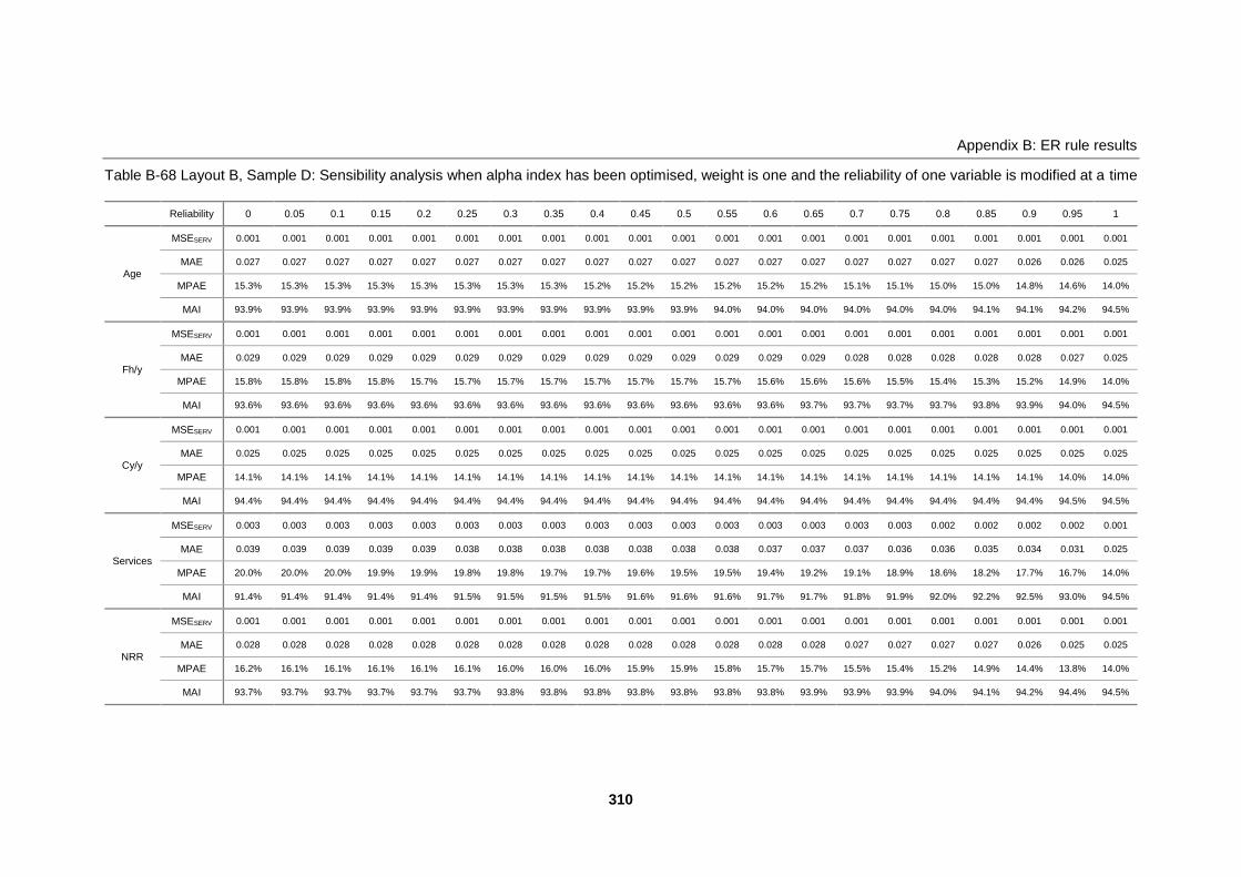
Appendix B: ER rule results
310
Table B-68 Layout B, Sample D: Sensibility analysis when alpha index has been optimised, weight is one and the reliability of one variable is modified at a time
Reliability 0 0.05 0.1 0.15 0.2 0.25 0.3 0.35 0.4 0.45 0.5 0.55 0.6 0.65 0.7 0.75 0.8 0.85 0.9 0.95 1
Age
MSESERV 0.001 0.001 0.001 0.001 0.001 0.001 0.001 0.001 0.001 0.001 0.001 0.001 0.001 0.001 0.001 0.001 0.001 0.001 0.001 0.001 0.001
MAE 0.027 0.027 0.027 0.027 0.027 0.027 0.027 0.027 0.027 0.027 0.027 0.027 0.027 0.027 0.027 0.027 0.027 0.027 0.026 0.026 0.025
MPAE 15.3% 15.3% 15.3% 15.3% 15.3% 15.3% 15.3% 15.3% 15.2% 15.2% 15.2% 15.2% 15.2% 15.2% 15.1% 15.1% 15.0% 15.0% 14.8% 14.6% 14.0%
MAI 93.9% 93.9% 93.9% 93.9% 93.9% 93.9% 93.9% 93.9% 93.9% 93.9% 93.9% 94.0% 94.0% 94.0% 94.0% 94.0% 94.0% 94.1% 94.1% 94.2% 94.5%
Fh/y
MSESERV 0.001 0.001 0.001 0.001 0.001 0.001 0.001 0.001 0.001 0.001 0.001 0.001 0.001 0.001 0.001 0.001 0.001 0.001 0.001 0.001 0.001
MAE 0.029 0.029 0.029 0.029 0.029 0.029 0.029 0.029 0.029 0.029 0.029 0.029 0.029 0.029 0.028 0.028 0.028 0.028 0.028 0.027 0.025
MPAE 15.8% 15.8% 15.8% 15.8% 15.7% 15.7% 15.7% 15.7% 15.7% 15.7% 15.7% 15.7% 15.6% 15.6% 15.6% 15.5% 15.4% 15.3% 15.2% 14.9% 14.0%
MAI 93.6% 93.6% 93.6% 93.6% 93.6% 93.6% 93.6% 93.6% 93.6% 93.6% 93.6% 93.6% 93.6% 93.7% 93.7% 93.7% 93.7% 93.8% 93.9% 94.0% 94.5%
Cy/y
MSESERV 0.001 0.001 0.001 0.001 0.001 0.001 0.001 0.001 0.001 0.001 0.001 0.001 0.001 0.001 0.001 0.001 0.001 0.001 0.001 0.001 0.001
MAE 0.025 0.025 0.025 0.025 0.025 0.025 0.025 0.025 0.025 0.025 0.025 0.025 0.025 0.025 0.025 0.025 0.025 0.025 0.025 0.025 0.025
MPAE 14.1% 14.1% 14.1% 14.1% 14.1% 14.1% 14.1% 14.1% 14.1% 14.1% 14.1% 14.1% 14.1% 14.1% 14.1% 14.1% 14.1% 14.1% 14.1% 14.0% 14.0%
MAI 94.4% 94.4% 94.4% 94.4% 94.4% 94.4% 94.4% 94.4% 94.4% 94.4% 94.4% 94.4% 94.4% 94.4% 94.4% 94.4% 94.4% 94.4% 94.4% 94.5% 94.5%
Services
MSESERV 0.003 0.003 0.003 0.003 0.003 0.003 0.003 0.003 0.003 0.003 0.003 0.003 0.003 0.003 0.003 0.003 0.002 0.002 0.002 0.002 0.001
MAE 0.039 0.039 0.039 0.039 0.039 0.038 0.038 0.038 0.038 0.038 0.038 0.038 0.037 0.037 0.037 0.036 0.036 0.035 0.034 0.031 0.025
MPAE 20.0% 20.0% 20.0% 19.9% 19.9% 19.8% 19.8% 19.7% 19.7% 19.6% 19.5% 19.5% 19.4% 19.2% 19.1% 18.9% 18.6% 18.2% 17.7% 16.7% 14.0%
MAI 91.4% 91.4% 91.4% 91.4% 91.4% 91.5% 91.5% 91.5% 91.5% 91.6% 91.6% 91.6% 91.7% 91.7% 91.8% 91.9% 92.0% 92.2% 92.5% 93.0% 94.5%
NRR
MSESERV 0.001 0.001 0.001 0.001 0.001 0.001 0.001 0.001 0.001 0.001 0.001 0.001 0.001 0.001 0.001 0.001 0.001 0.001 0.001 0.001 0.001
MAE 0.028 0.028 0.028 0.028 0.028 0.028 0.028 0.028 0.028 0.028 0.028 0.028 0.028 0.028 0.027 0.027 0.027 0.027 0.026 0.025 0.025
MPAE 16.2% 16.1% 16.1% 16.1% 16.1% 16.1% 16.0% 16.0% 16.0% 15.9% 15.9% 15.8% 15.7% 15.7% 15.5% 15.4% 15.2% 14.9% 14.4% 13.8% 14.0%
MAI 93.7% 93.7% 93.7% 93.7% 93.7% 93.7% 93.8% 93.8% 93.8% 93.8% 93.8% 93.8% 93.8% 93.9% 93.9% 93.9% 94.0% 94.1% 94.2% 94.4% 94.5%

Appendix B: ER rule results
311
Table B-69 Layout B (Four samples): MAI when alpha index has been optimised, weight is one and the reliability of one variable is modified at a time
Sample A
Sample B
Sample C
Sample D
91.5%
92.5%
93.5%
94.5%
95.5%
96.5%
0 0.1 0.2 0.3 0.4 0.5 0.6 0.7 0.8 0.9 1
MA
I
Reliability
Mean Accuracy Indicator per Variable
Age
Fh/y
Cy/y
Services
NRR
91.5%
92.5%
93.5%
94.5%
95.5%
96.5%
0 0.1 0.2 0.3 0.4 0.5 0.6 0.7 0.8 0.9 1
MA
I
Reliability
Mean Accuracy Indicator per Variable
Age
Fh/y
Cy/y
Services
NRR
91.0%
92.0%
93.0%
94.0%
95.0%
96.0%
0 0.1 0.2 0.3 0.4 0.5 0.6 0.7 0.8 0.9 1
MA
I
Reliability
Mean Accuracy Indicator per Variable
Age
Fh/y
Cy/y
Services
NRR
91.0%
92.0%
93.0%
94.0%
95.0%
0 0.1 0.2 0.3 0.4 0.5 0.6 0.7 0.8 0.9 1
MA
IReliability
Mean Accuracy Indicator per Variable
Age
Fh/y
Cy/y
Services
NRR

Appendix B: ER rule results
312
B.8.2 Sensitivity analysis when the reliability of all variables is modified equally at the same time
Table B-70 Layout A (Four samples): Sensibility analysis when alpha index has been optimised, weight is one and the reliability of all variables is modified
equally at the same time
Reliability 0 0.05 0.1 0.15 0.2 0.25 0.3 0.35 0.4 0.45 0.5 0.55 0.6 0.65 0.7 0.75 0.8 0.85 0.9 0.95 1
Sample A
MSESERV 0.002 0.002 0.002 0.002 0.002 0.002 0.002 0.002 0.002 0.002 0.002 0.002 0.002 0.002 0.002 0.002 0.002 0.001 0.001 0.001 0.000
MAE 0.040 0.040 0.040 0.040 0.039 0.039 0.039 0.039 0.038 0.038 0.037 0.036 0.036 0.035 0.034 0.032 0.030 0.028 0.025 0.021 0.016
MPAE 21.4% 21.3% 21.2% 21.0% 20.9% 20.7% 20.5% 20.3% 20.1% 19.8% 19.4% 19.1% 18.6% 18.0% 17.4% 16.6% 15.5% 14.1% 12.3% 10.3% 8.0%
MAI 90.5% 90.6% 90.6% 90.7% 90.7% 90.8% 90.9% 90.9% 91.0% 91.1% 91.3% 91.4% 91.6% 91.8% 92.1% 92.4% 92.8% 93.4% 94.2% 95.2% 96.3%
Sample B
MSESERV 0.002 0.002 0.002 0.002 0.002 0.002 0.002 0.002 0.002 0.002 0.002 0.002 0.002 0.002 0.002 0.001 0.001 0.001 0.001 0.001 0.000
MAE 0.039 0.038 0.038 0.038 0.038 0.037 0.037 0.037 0.036 0.036 0.035 0.034 0.034 0.033 0.032 0.030 0.028 0.026 0.023 0.019 0.016
MPAE 21.4% 21.3% 21.1% 21.0% 20.8% 20.6% 20.4% 20.2% 19.9% 19.6% 19.3% 18.9% 18.4% 17.8% 17.1% 16.3% 15.2% 13.8% 12.0% 10.1% 8.1%
MAI 90.9% 91.0% 91.0% 91.1% 91.2% 91.2% 91.3% 91.4% 91.5% 91.6% 91.7% 91.9% 92.1% 92.3% 92.6% 92.9% 93.3% 93.9% 94.6% 95.4% 96.3%
Sample C
MSESERV 0.002 0.002 0.002 0.002 0.002 0.002 0.002 0.002 0.002 0.002 0.002 0.002 0.002 0.002 0.002 0.001 0.001 0.001 0.001 0.001 0.000
MAE 0.039 0.038 0.038 0.038 0.038 0.037 0.037 0.036 0.036 0.035 0.035 0.034 0.033 0.032 0.031 0.030 0.028 0.026 0.023 0.019 0.015
MPAE 21.0% 20.9% 20.7% 20.5% 20.4% 20.1% 19.9% 19.6% 19.3% 19.0% 18.6% 18.2% 17.7% 17.1% 16.4% 15.6% 14.5% 13.1% 11.4% 9.7% 7.5%
MAI 90.9% 90.9% 91.0% 91.1% 91.1% 91.2% 91.3% 91.4% 91.5% 91.7% 91.8% 92.0% 92.2% 92.4% 92.7% 93.0% 93.4% 94.0% 94.7% 95.4% 96.6%
Sample D
MSESERV 0.002 0.002 0.002 0.002 0.002 0.002 0.002 0.002 0.002 0.002 0.002 0.002 0.002 0.002 0.002 0.002 0.001 0.001 0.001 0.001 0.000
MAE 0.039 0.039 0.039 0.039 0.038 0.038 0.038 0.037 0.037 0.036 0.036 0.035 0.034 0.034 0.032 0.031 0.029 0.027 0.023 0.020 0.015
MPAE 21.7% 21.6% 21.5% 21.3% 21.2% 21.0% 20.8% 20.6% 20.3% 20.0% 19.7% 19.3% 18.8% 18.2% 17.5% 16.6% 15.5% 14.1% 12.2% 10.3% 8.1%
MAI 90.8% 90.8% 90.9% 90.9% 91.0% 91.0% 91.1% 91.2% 91.3% 91.4% 91.6% 91.7% 91.9% 92.1% 92.4% 92.7% 93.2% 93.8% 94.5% 95.4% 96.4%

Appendix B: ER rule results
313
Table B-71 Layout B (Four samples): Sensibility analysis when alpha index has been optimised, weight is one and the reliability of all variables is modified
equally at the same time
Samples Reliability 0 0.05 0.1 0.15 0.2 0.25 0.3 0.35 0.4 0.45 0.5 0.55 0.6 0.65 0.7 0.75 0.8 0.85 0.9 0.95 1
Sample A
MSESERV 0.002 0.002 0.002 0.002 0.002 0.002 0.002 0.002 0.002 0.002 0.002 0.002 0.002 0.002 0.002 0.002 0.002 0.001 0.001 0.001 0.001
MAE 0.041 0.041 0.041 0.040 0.040 0.040 0.040 0.039 0.039 0.038 0.038 0.037 0.036 0.035 0.034 0.033 0.031 0.029 0.028 0.027 0.024
MPAE 21.3% 21.2% 21.1% 20.9% 20.8% 20.6% 20.4% 20.2% 20.0% 19.7% 19.4% 19.1% 18.6% 18.1% 17.6% 16.9% 16.1% 15.2% 14.4% 13.9% 12.9%
MAI 90.9% 90.9% 91.0% 91.0% 91.1% 91.1% 91.2% 91.3% 91.4% 91.5% 91.6% 91.8% 92.0% 92.2% 92.4% 92.7% 93.1% 93.5% 93.8% 94.0% 94.7%
Sample B
MSESERV 0.002 0.002 0.002 0.002 0.002 0.002 0.002 0.002 0.002 0.002 0.002 0.002 0.002 0.002 0.001 0.001 0.001 0.001 0.001 0.001 0.001
MAE 0.038 0.038 0.038 0.038 0.037 0.037 0.037 0.036 0.036 0.036 0.035 0.034 0.034 0.033 0.032 0.030 0.029 0.027 0.026 0.026 0.024
MPAE 20.8% 20.7% 20.6% 20.4% 20.3% 20.1% 19.9% 19.7% 19.5% 19.3% 19.0% 18.7% 18.3% 17.8% 17.2% 16.6% 15.8% 14.9% 14.3% 14.2% 13.4%
MAI 91.5% 91.5% 91.6% 91.6% 91.7% 91.7% 91.8% 91.9% 92.0% 92.1% 92.2% 92.3% 92.5% 92.7% 93.0% 93.3% 93.6% 93.9% 94.2% 94.3% 94.7%
Sample C
MSESERV 0.002 0.002 0.002 0.002 0.002 0.002 0.002 0.002 0.002 0.002 0.002 0.002 0.002 0.002 0.002 0.002 0.001 0.001 0.001 0.001 0.001
MAE 0.040 0.040 0.040 0.039 0.039 0.039 0.038 0.038 0.037 0.037 0.036 0.036 0.035 0.034 0.032 0.031 0.029 0.028 0.026 0.025 0.023
MPAE 21.3% 21.2% 21.0% 20.9% 20.7% 20.5% 20.3% 20.1% 19.8% 19.5% 19.1% 18.7% 18.3% 17.7% 17.0% 16.3% 15.5% 14.5% 13.5% 13.0% 12.6%
MAI 91.1% 91.2% 91.2% 91.3% 91.3% 91.4% 91.5% 91.6% 91.7% 91.8% 91.9% 92.1% 92.3% 92.5% 92.8% 93.1% 93.4% 93.9% 94.2% 94.5% 94.9%
Sample D
MSESERV 0.002 0.002 0.002 0.002 0.002 0.002 0.002 0.002 0.002 0.002 0.002 0.002 0.002 0.002 0.002 0.002 0.002 0.001 0.001 0.001 0.001
MAE 0.040 0.040 0.040 0.040 0.039 0.039 0.039 0.038 0.038 0.038 0.037 0.036 0.036 0.035 0.034 0.033 0.031 0.030 0.028 0.026 0.025
MPAE 21.6% 21.5% 21.4% 21.2% 21.1% 20.9% 20.8% 20.6% 20.3% 20.1% 19.8% 19.4% 19.0% 18.5% 18.0% 17.3% 16.6% 15.7% 14.8% 14.1% 14.0%
MAI 91.1% 91.1% 91.1% 91.2% 91.2% 91.3% 91.4% 91.5% 91.5% 91.7% 91.8% 91.9% 92.1% 92.3% 92.5% 92.8% 93.1% 93.4% 93.8% 94.1% 94.5%

Appendix B: ER rule results
314
Table B-72 Layout A and B (Four samples): MAI when alpha index has been optimised, weight is one and the reliability of all variables is modified equally at the
same time
Layout A
Layout B
90%
91%
92%
93%
94%
95%
96%
97%
0 0.1 0.2 0.3 0.4 0.5 0.6 0.7 0.8 0.9 1
MA
I
Reliability
Mean Accuracy Indicator Vs Reliablity
Sample A
Sample B
Sample C
Sample D
90%
91%
92%
93%
94%
95%
96%
97%
0 0.1 0.2 0.3 0.4 0.5 0.6 0.7 0.8 0.9 1
MA
I
Reliability
Mean Accuracy Indicator Vs Reliability
Sample A
Sample B
Sample C
Sample D

Appendix B: ER rule results
315
B.8.3 Sensitivity analysis modifying alpha-index, weight and reliability
Table B-73 Layout A (Four samples): Sensibility analysis when alpha index is one, weight is one and the reliability of all variables is modified equally at the same
time
Reliability 0 0.1 0.2 0.3 0.4 0.5 0.6 0.7 0.8 0.9 1
Sample A
MSESERV 0.002 0.002 0.002 0.002 0.002 0.002 0.002 0.001 0.001 0.001 0.001
MAE 0.037 0.036 0.035 0.035 0.033 0.032 0.030 0.028 0.026 0.023 0.017
MPAE 19.3% 18.9% 18.4% 17.9% 17.2% 16.4% 15.6% 14.6% 13.2% 11.8% 9.3%
MAI 91.3% 91.5% 91.7% 91.9% 92.1% 92.5% 92.8% 93.3% 93.9% 94.6% 96.0%
Sample B
MSESERV 0.002 0.002 0.002 0.002 0.002 0.002 0.001 0.001 0.001 0.001 0.001
MAE 0.035 0.035 0.034 0.033 0.032 0.031 0.029 0.027 0.024 0.022 0.018
MPAE 19.3% 18.9% 18.5% 17.9% 17.2% 16.5% 15.5% 14.3% 12.7% 11.6% 9.7%
MAI 91.7% 91.9% 92.0% 92.3% 92.5% 92.8% 93.2% 93.7% 94.4% 94.9% 95.8%
Sample C
MSESERV 0.002 0.002 0.002 0.002 0.002 0.001 0.001 0.001 0.001 0.001 0.001
MAE 0.035 0.035 0.034 0.033 0.032 0.030 0.029 0.027 0.024 0.022 0.017
MPAE 18.9% 18.4% 17.9% 17.3% 16.6% 15.8% 14.9% 13.7% 12.3% 11.0% 8.9%
MAI 91.7% 91.8% 92.0% 92.3% 92.5% 92.8% 93.2% 93.7% 94.3% 94.8% 95.9%
Sample D
MSESERV 0.002 0.002 0.002 0.002 0.002 0.002 0.002 0.002 0.001 0.001 0.000
MAE 0.039 0.039 0.038 0.038 0.037 0.036 0.034 0.032 0.029 0.023 0.015
MPAE 21.7% 21.5% 21.2% 20.8% 20.3% 19.7% 18.8% 17.5% 15.5% 12.2% 8.1%
MAI 90.8% 90.9% 91.0% 91.1% 91.3% 91.6% 91.9% 92.4% 93.2% 94.5% 96.4%

Appendix B: ER rule results
316
Table B-74 Layout A (Four samples): Sensibility analysis when alpha index is one, weight is optimised and the reliability of all variables is modified equally at
the same time
Reliability 0 0.1 0.2 0.3 0.4 0.5 0.6 0.7 0.8 0.9 1
Sample A
MSESERV 0.001 0.001 0.001 0.001 0.001 0.001 0.001 0.001 0.001 0.001 0.001
MAE 0.022 0.022 0.022 0.021 0.021 0.021 0.021 0.021 0.021 0.021 0.017
MPAE 11.3% 11.2% 11.2% 11.2% 11.1% 11.0% 10.9% 10.8% 10.6% 10.7% 9.3%
MAI 94.9% 94.9% 94.9% 95.0% 95.0% 95.0% 95.0% 95.1% 95.2% 95.1% 96.0%
Sample B
MSESERV 0.001 0.001 0.001 0.001 0.001 0.001 0.001 0.001 0.001 0.001 0.001
MAE 0.016 0.016 0.016 0.020 0.016 0.016 0.016 0.020 0.020 0.017 0.018
MPAE 8.9% 8.9% 8.8% 11.0% 8.8% 8.7% 8.7% 10.8% 10.7% 9.0% 9.7%
MAI 96.2% 96.2% 96.2% 95.3% 96.2% 96.2% 96.2% 95.3% 95.4% 96.1% 95.8%
Sample C
MSESERV 0.001 0.001 0.001 0.001 0.001 0.001 0.001 0.001 0.001 0.001 0.001
MAE 0.016 0.017 0.016 0.016 0.016 0.019 0.017 0.019 0.019 0.015 0.017
MPAE 8.0% 8.6% 8.1% 8.2% 8.0% 9.8% 8.5% 9.6% 9.6% 7.8% 8.9%
MAI 96.3% 96.1% 96.3% 96.3% 96.3% 95.6% 96.1% 95.6% 95.6% 96.4% 95.9%
Sample D
MSESERV 0.001 0.001 0.001 0.001 0.001 0.001 0.001 0.001 0.001 0.001 0.000
MAE 0.022 0.022 0.022 0.022 0.022 0.022 0.022 0.018 0.021 0.019 0.015
MPAE 11.6% 11.6% 11.6% 11.6% 11.6% 11.6% 11.6% 9.7% 11.5% 10.1% 8.1%
MAI 94.9% 94.9% 94.9% 94.9% 94.9% 94.9% 94.9% 95.7% 94.9% 95.6% 96.4%

Appendix B: ER rule results
317
Table B-75 Layout A (Four samples): Sensibility analysis when alpha index is optimised, weight is one and the reliability of all variables is modified equally at
the same time
Reliability 0 0.1 0.2 0.3 0.4 0.5 0.6 0.7 0.8 0.9 1
Sample A
MSESERV 0.002 0.002 0.002 0.002 0.002 0.002 0.002 0.002 0.002 0.001 0.000
MAE 0.040 0.040 0.039 0.039 0.038 0.037 0.036 0.034 0.030 0.025 0.016
MPAE 21.4% 21.2% 20.9% 20.5% 20.1% 19.4% 18.6% 17.4% 15.5% 12.3% 8.0%
MAI 90.5% 90.6% 90.7% 90.9% 91.0% 91.3% 91.6% 92.1% 92.8% 94.2% 96.3%
Sample B
MSESERV 0.002 0.002 0.002 0.002 0.002 0.002 0.002 0.002 0.001 0.001 0.000
MAE 0.039 0.038 0.038 0.037 0.036 0.035 0.034 0.032 0.028 0.023 0.016
MPAE 21.4% 21.1% 20.8% 20.4% 19.9% 19.3% 18.4% 17.1% 15.2% 12.0% 8.1%
MAI 90.9% 91.0% 91.2% 91.3% 91.5% 91.7% 92.1% 92.6% 93.3% 94.6% 96.3%
Sample C
MSESERV 0.002 0.002 0.002 0.002 0.002 0.002 0.002 0.002 0.001 0.001 0.000
MAE 0.039 0.038 0.038 0.037 0.036 0.035 0.033 0.031 0.028 0.023 0.015
MPAE 21.0% 20.7% 20.4% 19.9% 19.3% 18.6% 17.7% 16.4% 14.5% 11.4% 7.5%
MAI 90.9% 91.0% 91.1% 91.3% 91.5% 91.8% 92.2% 92.7% 93.4% 94.7% 96.6%
Sample D
MSESERV 0.002 0.002 0.002 0.002 0.002 0.002 0.001 0.001 0.001 0.001 0.001
MAE 0.036 0.035 0.034 0.033 0.032 0.031 0.029 0.027 0.025 0.023 0.017
MPAE 19.5% 19.1% 18.6% 18.0% 17.3% 16.4% 15.4% 14.3% 13.0% 11.8% 9.4%
MAI 91.6% 91.7% 91.9% 92.1% 92.4% 92.7% 93.1% 93.6% 94.1% 94.7% 95.9%

Appendix B: ER rule results
318
Table B-76 Layout A (Four samples): Sensibility analysis when alpha index is optimised, weight is optimised and the reliability of all variables is modified equally
at the same time
Reliability 0 0.1 0.2 0.3 0.4 0.5 0.6 0.7 0.8 0.9 1
Sample A
MSESERV 0.001 0.001 0.001 0.001 0.001 0.001 0.001 0.001 0.001 0.001 0.000
MAE 0.022 0.022 0.022 0.022 0.022 0.022 0.022 0.021 0.021 0.017 0.016
MPAE 11.4% 11.4% 11.3% 11.3% 11.3% 11.2% 11.2% 11.1% 10.9% 8.9% 8.0%
MAI 94.9% 94.9% 94.9% 94.9% 94.9% 94.9% 94.9% 95.0% 95.0% 95.9% 96.3%
Sample B
MSESERV 0.001 0.001 0.001 0.001 0.001 0.001 0.001 0.001 0.001 0.001 0.000
MAE 0.020 0.016 0.016 0.016 0.016 0.016 0.020 0.016 0.017 0.017 0.016
MPAE 11.0% 8.8% 8.7% 8.8% 8.8% 8.8% 11.1% 8.8% 9.3% 9.1% 8.1%
MAI 95.3% 96.2% 96.2% 96.2% 96.2% 96.2% 95.2% 96.2% 96.0% 96.1% 96.3%
Sample C
MSESERV 0.001 0.001 0.001 0.001 0.001 0.001 0.001 0.001 0.001 0.001 0.000
MAE 0.016 0.016 0.016 0.016 0.016 0.016 0.016 0.016 0.016 0.019 0.015
MPAE 8.1% 8.1% 8.2% 8.1% 8.1% 8.0% 8.1% 8.0% 8.0% 9.5% 7.5%
MAI 96.3% 96.3% 96.3% 96.3% 96.3% 96.3% 96.3% 96.4% 96.3% 95.6% 96.6%
Sample D
MSESERV 0.001 0.001 0.001 0.001 0.001 0.001 0.001 0.001 0.001 0.001 0.001
MAE 0.022 0.022 0.022 0.022 0.022 0.022 0.022 0.018 0.018 0.017 0.017
MPAE 11.7% 11.7% 11.7% 11.7% 11.7% 11.7% 11.7% 9.8% 9.6% 9.3% 9.4%
MAI 94.8% 94.8% 94.8% 94.8% 94.8% 94.8% 94.9% 95.7% 95.8% 95.9% 95.9%

Appendix B: ER rule results
319
Table B-77 Layout A (Four samples): MAI comparison when alpha index and weight are one and then optimised, and the reliability of all variables is modified
equally at the same time
Layout A Sample A
Layout A Sample B
Layout A Sample C
Layout A Sample D
90%
91%
92%
93%
94%
95%
96%
97%
0 0.1 0.2 0.3 0.4 0.5 0.6 0.7 0.8 0.9 1
MA
I
Reliability
MAI vs ReliabilityAlpha=1 and OptimisedWeight=1 and Optimised
Alpha = Optimised, W = 1 Alpha = Optimised, W = Optimised
Alpha = 1, W = 1 Alpha = 1, W = Optimised
90%
91%
92%
93%
94%
95%
96%
97%
0 0.1 0.2 0.3 0.4 0.5 0.6 0.7 0.8 0.9 1
MA
I
Reliability
MAI vs ReliabilityAlpha=1 and OptimisedWeight=1 and Optimised
Alpha=Optimised, W=1 Alpha=Optimised, W=Optimised
Alpha=1, W=1 Alpha=1, W=Optimised
90%
91%
92%
93%
94%
95%
96%
97%
0 0.1 0.2 0.3 0.4 0.5 0.6 0.7 0.8 0.9 1
MA
I
Reliability
MAI vs ReliabilityAlpha=1 and OptimisedWeight=1 and Optimised
Alpha=Optimised, W=1 Alpha=Optimised, W=Optimised
Alpha=1, W=1 Alpha=1, W=Optimised
90%
91%
92%
93%
94%
95%
96%
97%
0 0.1 0.2 0.3 0.4 0.5 0.6 0.7 0.8 0.9 1
MA
I
Reliability
MAI vs ReliabilityAlpha=1 and OptimisedWeight=1 and Optimised
Alpha=Optimised, W=1 Alpha=Optimised, W=Optimised
Alpha=1, W=1 Alpha=1, W=Optimised

Appendix B: ER rule results
320
Table B-78 Layout B (Four samples): Sensibility analysis when alpha index is one, weight is one and the reliability of all variables is modified equally at the same
Reliability 0 0.1 0.2 0.3 0.4 0.5 0.6 0.7 0.8 0.9 1
Sample A
MSESERV 0.002 0.002 0.002 0.002 0.002 0.002 0.002 0.002 0.001 0.001 0.001
MAE 0.038 0.038 0.037 0.036 0.035 0.034 0.033 0.032 0.030 0.029 0.024
MPAE 19.6% 19.2% 18.8% 18.3% 17.8% 17.3% 16.8% 16.2% 15.5% 15.1% 12.8%
MAI 91.5% 91.6% 91.8% 91.9% 92.1% 92.4% 92.7% 93.0% 93.3% 93.6% 94.6%
Sample B
MSESERV 0.002 0.002 0.002 0.002 0.002 0.002 0.001 0.001 0.001 0.001 0.001
MAE 0.036 0.036 0.035 0.034 0.033 0.032 0.031 0.029 0.028 0.027 0.024
MPAE 19.3% 19.0% 18.6% 18.2% 17.7% 17.2% 16.6% 15.9% 15.2% 14.8% 13.5%
MAI 91.9% 92.1% 92.2% 92.4% 92.6% 92.8% 93.1% 93.5% 93.8% 94.1% 94.6%
Sample C
MSESERV 0.002 0.002 0.002 0.002 0.002 0.002 0.002 0.001 0.001 0.001 0.001
MAE 0.037 0.037 0.036 0.035 0.034 0.033 0.031 0.030 0.028 0.026 0.023
MPAE 19.4% 18.9% 18.5% 18.0% 17.4% 16.8% 16.2% 15.5% 14.6% 13.8% 12.1%
MAI 91.7% 91.9% 92.1% 92.3% 92.5% 92.7% 93.0% 93.4% 93.9% 94.3% 94.9%
Sample D
MSESERV 0.002 0.002 0.002 0.002 0.002 0.002 0.002 0.002 0.001 0.001 0.001
MAE 0.038 0.037 0.036 0.036 0.035 0.033 0.032 0.031 0.030 0.028 0.025
MPAE 19.8% 19.5% 19.0% 18.5% 18.0% 17.4% 16.9% 16.4% 15.9% 15.4% 13.7%
MAI 91.6% 91.7% 91.9% 92.1% 92.3% 92.6% 92.8% 93.1% 93.4% 93.7% 94.4%

Appendix B: ER rule results
321
Table B-79 Layout B (Four samples): Sensibility analysis when alpha index is one, weight is optimised and the reliability of all variables is modified equally at
the same time
Reliability 0 0.1 0.2 0.3 0.4 0.5 0.6 0.7 0.8 0.9 1
Sample A
MSESERV 0.001 0.001 0.001 0.001 0.001 0.001 0.001 0.001 0.001 0.001 0.001
MAE 0.025 0.025 0.024 0.025 0.025 0.025 0.025 0.025 0.022 0.025 0.024
MPAE 12.6% 12.6% 12.1% 12.6% 12.6% 12.6% 12.6% 12.7% 11.5% 12.4% 12.8%
MAI 94.4% 94.4% 94.8% 94.4% 94.4% 94.4% 94.4% 94.4% 95.0% 94.5% 94.6%
Sample B
MSESERV 0.001 0.001 0.001 0.001 0.001 0.001 0.001 0.001 0.001 0.001 0.001
MAE 0.020 0.020 0.020 0.022 0.020 0.020 0.020 0.020 0.020 0.020 0.024
MPAE 10.6% 10.7% 10.4% 11.7% 10.7% 10.4% 10.7% 10.5% 10.6% 10.6% 13.5%
MAI 95.6% 95.5% 95.6% 95.1% 95.6% 95.6% 95.6% 95.6% 95.6% 95.6% 94.6%
Sample C
MSESERV 0.001 0.001 0.001 0.001 0.001 0.001 0.001 0.001 0.001 0.001 0.001
MAE 0.020 0.020 0.020 0.023 0.020 0.027 0.020 0.020 0.023 0.023 0.023
MPAE 10.0% 9.9% 9.9% 11.5% 9.8% 13.5% 10.1% 9.9% 11.5% 11.6% 12.1%
MAI 95.5% 95.6% 95.5% 94.9% 95.6% 94.0% 95.5% 95.6% 95.0% 94.9% 94.9%
Sample D
MSESERV 0.001 0.001 0.001 0.001 0.001 0.001 0.001 0.001 0.001 0.001 0.001
MAE 0.024 0.024 0.024 0.024 0.024 0.024 0.024 0.024 0.021 0.026 0.025
MPAE 12.2% 12.2% 12.2% 12.2% 12.2% 12.2% 12.2% 12.1% 11.4% 13.7% 13.7%
MAI 94.7% 94.7% 94.7% 94.7% 94.7% 94.7% 94.7% 94.8% 95.3% 94.3% 94.4%
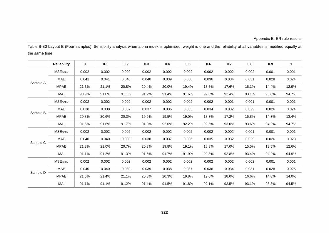
Appendix B: ER rule results
322
Table B-80 Layout B (Four samples): Sensibility analysis when alpha index is optimised, weight is one and the reliability of all variables is modified equally at
the same time
Reliability 0 0.1 0.2 0.3 0.4 0.5 0.6 0.7 0.8 0.9 1
Sample A
MSESERV 0.002 0.002 0.002 0.002 0.002 0.002 0.002 0.002 0.002 0.001 0.001
MAE 0.041 0.041 0.040 0.040 0.039 0.038 0.036 0.034 0.031 0.028 0.024
MPAE 21.3% 21.1% 20.8% 20.4% 20.0% 19.4% 18.6% 17.6% 16.1% 14.4% 12.9%
MAI 90.9% 91.0% 91.1% 91.2% 91.4% 91.6% 92.0% 92.4% 93.1% 93.8% 94.7%
Sample B
MSESERV 0.002 0.002 0.002 0.002 0.002 0.002 0.002 0.001 0.001 0.001 0.001
MAE 0.038 0.038 0.037 0.037 0.036 0.035 0.034 0.032 0.029 0.026 0.024
MPAE 20.8% 20.6% 20.3% 19.9% 19.5% 19.0% 18.3% 17.2% 15.8% 14.3% 13.4%
MAI 91.5% 91.6% 91.7% 91.8% 92.0% 92.2% 92.5% 93.0% 93.6% 94.2% 94.7%
Sample C
MSESERV 0.002 0.002 0.002 0.002 0.002 0.002 0.002 0.002 0.001 0.001 0.001
MAE 0.040 0.040 0.039 0.038 0.037 0.036 0.035 0.032 0.029 0.026 0.023
MPAE 21.3% 21.0% 20.7% 20.3% 19.8% 19.1% 18.3% 17.0% 15.5% 13.5% 12.6%
MAI 91.1% 91.2% 91.3% 91.5% 91.7% 91.9% 92.3% 92.8% 93.4% 94.2% 94.9%
Sample D
MSESERV 0.002 0.002 0.002 0.002 0.002 0.002 0.002 0.002 0.002 0.001 0.001
MAE 0.040 0.040 0.039 0.039 0.038 0.037 0.036 0.034 0.031 0.028 0.025
MPAE 21.6% 21.4% 21.1% 20.8% 20.3% 19.8% 19.0% 18.0% 16.6% 14.8% 14.0%
MAI 91.1% 91.1% 91.2% 91.4% 91.5% 91.8% 92.1% 92.5% 93.1% 93.8% 94.5%

Appendix B: ER rule results
323
Table B-81 Layout B (Four samples): Sensibility analysis when alpha index is optimised, weight is optimised and the reliability of all variables is modified equally
at the same time
Reliability 0 0.1 0.2 0.3 0.4 0.5 0.6 0.7 0.8 0.9 1
Sample A
MSESERV 0.001 0.001 0.001 0.001 0.001 0.001 0.001 0.001 0.001 0.001 0.001
MAE 0.025 0.025 0.025 0.025 0.025 0.025 0.025 0.023 0.025 0.022 0.024
MPAE 12.6% 12.6% 12.6% 12.6% 12.6% 12.6% 12.6% 12.0% 12.6% 11.5% 12.9%
MAI 94.4% 94.4% 94.4% 94.4% 94.4% 94.4% 94.4% 94.8% 94.4% 95.1% 94.7%
Sample B
MSESERV 0.001 0.001 0.001 0.001 0.001 0.001 0.001 0.001 0.001 0.001 0.001
MAE 0.020 0.020 0.020 0.020 0.020 0.022 0.020 0.020 0.020 0.020 0.024
MPAE 10.6% 10.7% 10.6% 10.6% 10.6% 11.7% 10.6% 10.4% 10.6% 10.5% 13.4%
MAI 95.6% 95.6% 95.6% 95.6% 95.6% 95.1% 95.6% 95.6% 95.6% 95.6% 94.7%
Sample C
MSESERV 0.001 0.001 0.001 0.001 0.001 0.001 0.001 0.001 0.001 0.001 0.001
MAE 0.020 0.021 0.020 0.020 0.020 0.020 0.020 0.020 0.020 0.020 0.023
MPAE 9.8% 10.6% 9.7% 9.7% 9.8% 9.8% 9.8% 9.8% 9.8% 9.8% 12.6%
MAI 95.7% 95.2% 95.6% 95.6% 95.6% 95.6% 95.6% 95.6% 95.6% 95.6% 94.9%
Sample D
MSESERV 0.001 0.001 0.001 0.001 0.001 0.001 0.001 0.001 0.001 0.001 0.001
MAE 0.024 0.024 0.024 0.024 0.024 0.024 0.021 0.024 0.024 0.021 0.025
MPAE 12.3% 12.2% 12.2% 12.3% 12.2% 12.2% 11.0% 12.2% 12.2% 10.9% 14.0%
MAI 94.7% 94.7% 94.7% 94.7% 94.7% 94.7% 95.3% 94.7% 94.7% 95.3% 94.5%

Appendix B: ER rule results
324
Table B-82 Layout B (Four samples): MAI comparison when alpha index and weight are one and then optimised, and the reliability of all variables is modified
equally at the same time
Layout B Sample A
Layout B Sample B
Layout B Sample C
Layout B Sample D
90%
91%
92%
93%
94%
95%
96%
97%
0 0.1 0.2 0.3 0.4 0.5 0.6 0.7 0.8 0.9 1
MA
I
Reliability
MAI vs ReliabilityAlpha=1 and OptimisedWeight=1 and Optimised
Alpha=Optimised, W=1 Alpha=Optimised, W=Optimised
Alpha=1, W=1 Alpha=1, W=Optimised
91%
92%
93%
94%
95%
96%
97%
0 0.1 0.2 0.3 0.4 0.5 0.6 0.7 0.8 0.9 1
MA
I
Reliability
MAI vs ReliabilityAlpha=1 and OptimisedWeight=1 and Optimised
Alpha=Optimised, W=1 Alpha=Optimised, W=Optimised
Alpha=1, W=1 Alpha=1, W=Optimised
90%
91%
92%
93%
94%
95%
96%
97%
0 0.1 0.2 0.3 0.4 0.5 0.6 0.7 0.8 0.9 1
MA
I
Reliability
MAI vs ReliabilityAlpha=1 and OptimisedWeight=1 and Optimised
Alpha=Optimised, W=1 Alpha=Optimised, W=Optimised
Alpha=1, W=1 Alpha=1, W=Optimised
90%
91%
92%
93%
94%
95%
96%
97%
0 0.1 0.2 0.3 0.4 0.5 0.6 0.7 0.8 0.9 1
MA
I
Reliability
MAI vs ReliabilityAlpha=1 and OptimisedWeight=1 and Optimised
Alpha=Optimised, W=1 Alpha=Optimised, W=Optimised
Alpha=1, W=1 Alpha=1, W=Optimised

Appendix B: ER rule results
325
B.9 Validation results
Table B-83 Layout A: Model performance comparison of the training and validation groups and all the dataset
Training Group Validation Group All Data
Sample A Sample B Sample C Sample D Sample A Sample B Sample C Sample D Sample A Sample B Sample C Sample D
MSESERV 0.0009 0.0006 0.0005 0.0007 0.0021 0.0027 0.0030 0.0009 0.0010 0.0009 0.0008 0.0007
MAE 0.0203 0.0167 0.0154 0.0176 0.0356 0.0413 0.0428 0.0237 0.0221 0.0197 0.0187 0.0183
MAPE 10.3% 9.1% 7.8% 9.6% 24.1% 18.6% 24.3% 13.3% 12.0% 10.3% 9.8% 10.0%
MAI 95.2% 96.1% 96.4% 95.9% 91.6% 90.3% 89.9% 94.4% 94.8% 95.4% 95.6% 95.7%
Figure B-32 Layout A: MAI comparison for training and validation groups and for the whole sample
95.2%96.1% 96.4%
95.9%
91.6%
90.3% 89.9%
94.4% 94.8%95.4% 95.6% 95.7%
86.0%
88.0%
90.0%
92.0%
94.0%
96.0%
98.0%
S1 S2 S3 S4 S1 S2 S3 S4 S1 S2 S3 S4
Training Validation All
MAI of Training, Validation and All Data-points

Appendix B: ER rule results
326
Table B-84 Layout B: Model performance comparison of the training and validation groups and all the dataset
Training Group Validation Group All Data
Sample A Sample B Sample C Sample D Sample A Sample B Sample C Sample D Sample A Sample B Sample C Sample D
MSESERV 0.0011 0.0008 0.0009 0.0010 0.0011 0.0024 0.0031 0.0013 0.0011 0.0010 0.0011 0.0010
MAE 0.0243 0.0195 0.0198 0.0208 0.0235 0.0374 0.0444 0.0315 0.0242 0.0216 0.0228 0.0221
MAPE 12.1% 10.3% 9.8% 10.9% 15.5% 17.3% 24.8% 16.8% 12.5% 11.2% 11.6% 11.6%
MAI 94.6% 95.7% 95.6% 95.4% 94.8% 91.7% 90.1% 93.0% 94.6% 95.2% 94.9% 95.1%
Figure B-33 Layout B: MAI comparison for training and validation groups and for the whole sample
94.6%
95.7% 95.6% 95.4%94.8%
91.7%
90.1%
93.0%
94.6%95.2% 94.9% 95.1%
86.0%
88.0%
90.0%
92.0%
94.0%
96.0%
98.0%
S1 S2 S3 S4 S1 S2 S3 S4 S1 S2 S3 S4
Training Validation All
MAI of Training, Validation and All Data-points