Analysing uplink performance in relay-enabled LTE-networks · To catch up with this enormous rise in cellular traffic, ... Cellular network with relay. ... GSM/UMTS networks if the

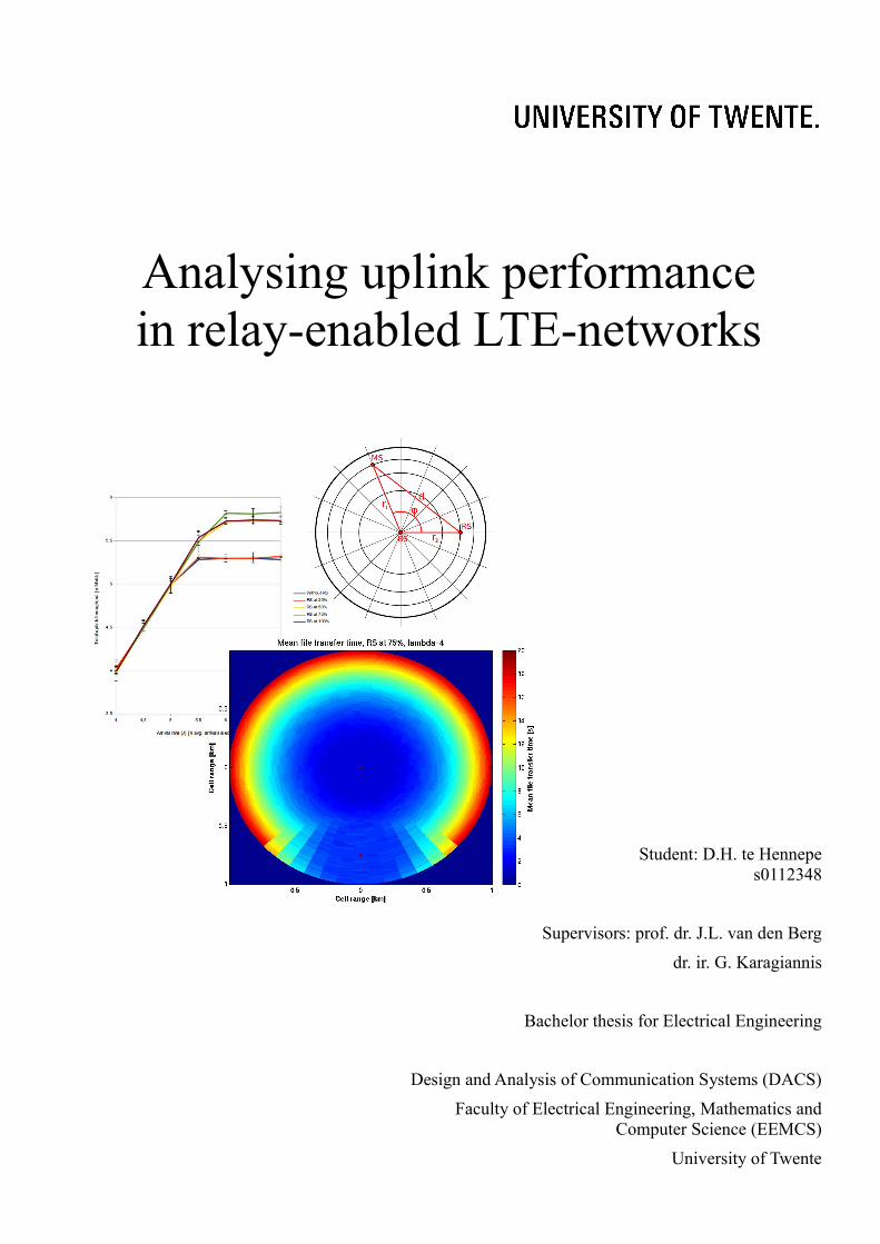
Student: D.H. te Hennepes0112348

Supervisors: prof. dr. J.L. van den Berg

dr. ir. G. Karagiannis

Bachelor thesis for Electrical Engineering

Design and Analysis of Communication Systems (DACS)

Faculty of Electrical Engineering, Mathematics andComputer Science (EEMCS)

University of Twente

Analysing uplink performance in relay-enabled LTE-networks

Table of Contents

List of abbreviations.............................................................................................................................5

Chapter 1. Introduction.......................................................................................................................71.1 Problem statement.......................................................................................................................81.2 Research questions and approach................................................................................................9

Chapter 2. LTE Networks..................................................................................................................112.1 General overview.......................................................................................................................112.2 eNode-B.....................................................................................................................................132.3 Air interface...............................................................................................................................132.4 Uplink scheduling......................................................................................................................14

2.4.1 Operation............................................................................................................................142.4.2 Algorithms..........................................................................................................................15

2.5 Signal theory..............................................................................................................................162.5.1 Received signal strength....................................................................................................162.5.2 Interference and noise........................................................................................................172.5.3 Data rate.............................................................................................................................18

Chapter 3. Relaying in LTE-networks..............................................................................................193.1 Advantages of using a relay.......................................................................................................193.2 Relaying in LTE.........................................................................................................................193.4 Uplink scheduling with relaying................................................................................................213.5 Related work..............................................................................................................................22

Chapter 4. Performance modelling and analysis.............................................................................254.1 Network scenario, performance measures and approach..........................................................25

4.1.1 Network scenario...............................................................................................................254.1.2 Performance measures.......................................................................................................254.1.3 Approach............................................................................................................................26

4.2 Performance Model...................................................................................................................264.2.1 Determining zones and sectors..........................................................................................264.2.2 Determining data rate.........................................................................................................274.2.3 Deciding when to use the relay..........................................................................................27

3

List of abbreviations

4.2.4 Flow dynamics...................................................................................................................294.2.5 Simulation..........................................................................................................................29

Chapter 5. Experiments and discussions..........................................................................................315.1 Experiment 1. Service area of the Relay Station.......................................................................31

5.1.1 Parameter settings..............................................................................................................315.1.2 Experiment setup...............................................................................................................315.1.3 Method...............................................................................................................................325.1.4 Results................................................................................................................................325.1.5 Discussion..........................................................................................................................32

5.2 Experiment 2. Total uplink throughput and impact on cell capacity.........................................345.2.1 Parameter settings..............................................................................................................345.2.2 Experiment setup...............................................................................................................345.2.3 Method...............................................................................................................................345.2.4 Results................................................................................................................................345.2.5 Discussion..........................................................................................................................34

5.3 Experiment 3. Impact of RS position on mean file transfer time per segment..........................365.3.1 Parameter settings..............................................................................................................365.3.2 Experiment setup...............................................................................................................365.3.3 Method...............................................................................................................................365.3.4 Results................................................................................................................................365.3.5 Discussion..........................................................................................................................41

Chapter 6. Conclusion and future work...........................................................................................43

Chapter 7. References........................................................................................................................45

Appendix A. Matlab code..................................................................................................................47

4



3GPP 3rd Generation Partnership Project

AF Amplify & Forward

BS Base Station

DF Decode & Forward

E-UTRAN Evolved UMTS Terrestrial Radio Access Network

EPC Evolved Packet Core

FFA Fair Fixed Assignment

FWC Fair Work Conserving

HSS Home Subscriber Server

LTE Long Term Evolution

MAV Maximum Added Value

MME Mobile Management Entity

MS Mobile Station

O-FDMA Orthogonal Frequency Division Multiple Access

PAPR Peak-to-Average-Power Ratio

PGW PDN-GW, Packet Data Network Gateway

RB Resource Block

RIV Resource Indication Value

RS Relay Station

SC-FDMA Single-Carrier Frequency Division Multiple Access

SGW Serving Gateway

UMTS Universal Mobile Telecommunications System

WCDMA Wideband Code Division Multiple Access

5

Chapter 1. Introduction


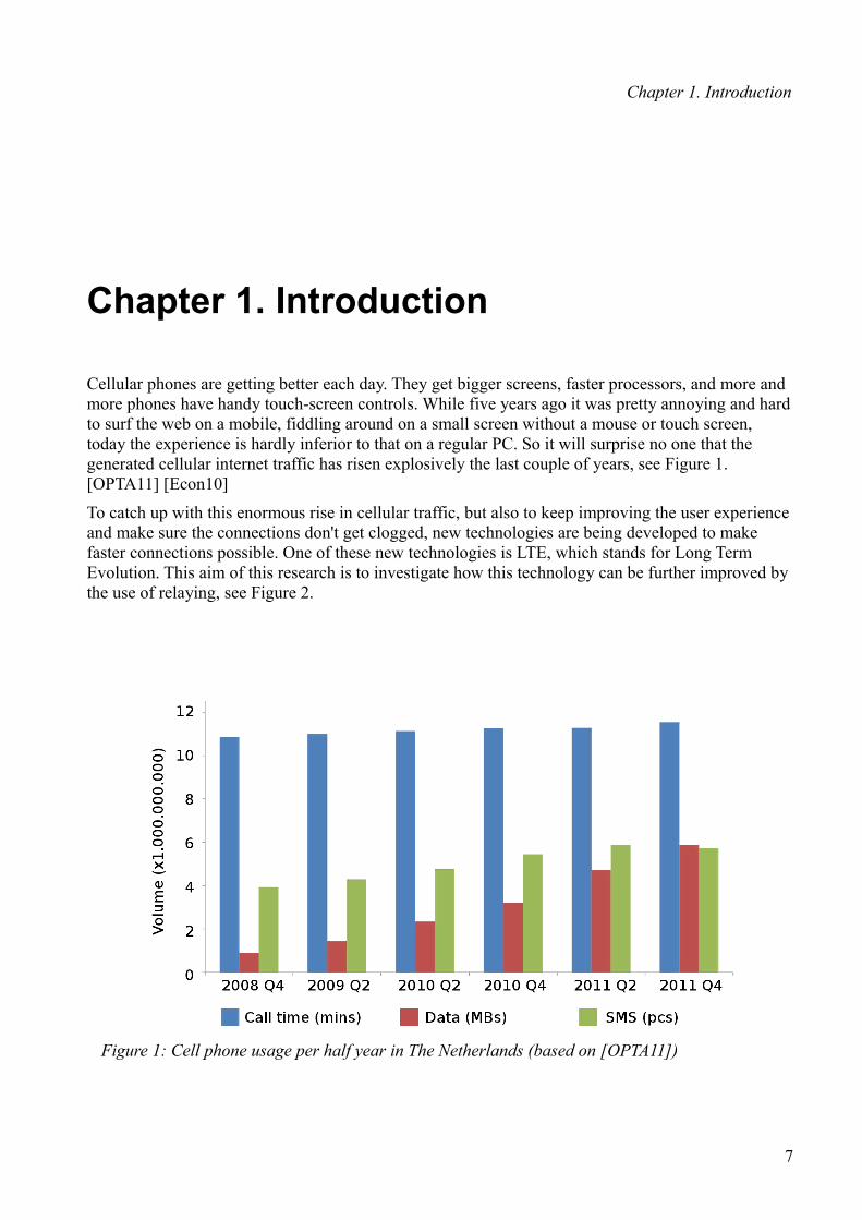
Cellular phones are getting better each day. They get bigger screens, faster processors, and more and more phones have handy touch-screen controls. While five years ago it was pretty annoying and hard to surf the web on a mobile, fiddling around on a small screen without a mouse or touch screen, today the experience is hardly inferior to that on a regular PC. So it will surprise no one that the generated cellular internet traffic has risen explosively the last couple of years, see Figure 1. [OPTA11] [Econ10]

To catch up with this enormous rise in cellular traffic, but also to keep improving the user experience and make sure the connections don't get clogged, new technologies are being developed to make faster connections possible. One of these new technologies is LTE, which stands for Long Term Evolution. This aim of this research is to investigate how this technology can be further improved by the use of relaying, see Figure 2.

7

Figure 1: Cell phone usage per half year in The Netherlands (based on [OPTA11])


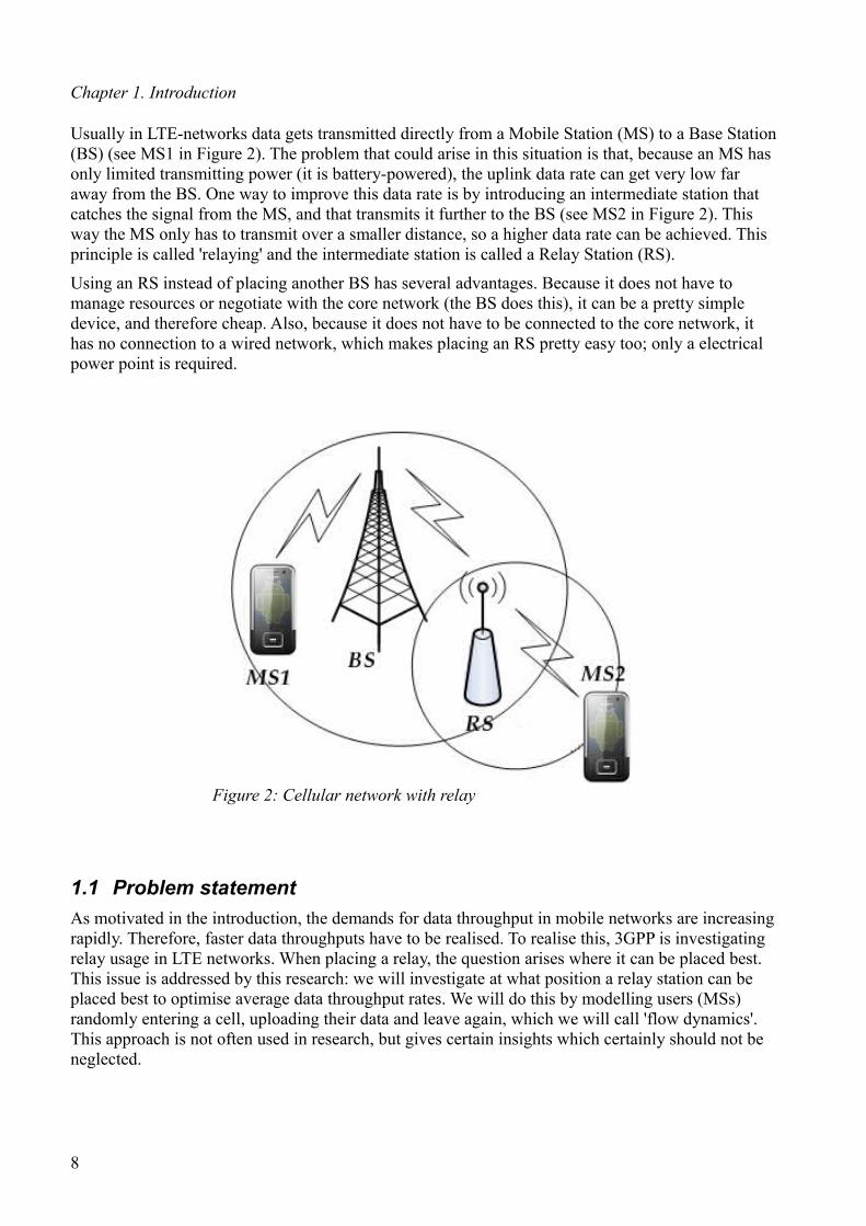
Usually in LTE-networks data gets transmitted directly from a Mobile Station (MS) to a Base Station (BS) (see MS1 in Figure 2). The problem that could arise in this situation is that, because an MS has only limited transmitting power (it is battery-powered), the uplink data rate can get very low far away from the BS. One way to improve this data rate is by introducing an intermediate station that catches the signal from the MS, and that transmits it further to the BS (see MS2 in Figure 2). This way the MS only has to transmit over a smaller distance, so a higher data rate can be achieved. This principle is called 'relaying' and the intermediate station is called a Relay Station (RS).

Using an RS instead of placing another BS has several advantages. Because it does not have to manage resources or negotiate with the core network (the BS does this), it can be a pretty simple device, and therefore cheap. Also, because it does not have to be connected to the core network, it has no connection to a wired network, which makes placing an RS pretty easy too; only a electrical power point is required.

1.1 Problem statementAs motivated in the introduction, the demands for data throughput in mobile networks are increasing rapidly. Therefore, faster data throughputs have to be realised. To realise this, 3GPP is investigating relay usage in LTE networks. When placing a relay, the question arises where it can be placed best. This issue is addressed by this research: we will investigate at what position a relay station can be placed best to optimise average data throughput rates. We will do this by modelling users (MSs) randomly entering a cell, uploading their data and leave again, which we will call 'flow dynamics'. This approach is not often used in research, but gives certain insights which certainly should not be neglected.

8

Figure 2: Cellular network with relay


1.2 Research questions and approachIn order to investigate this problem, the following research questions are derived:

1. How does the LTE uplink resource management operate?2. What are the assumptions and requirements on the uplink imposed by the RS?3. Which performance models can be used to analyse the effect an RS on the uplink

performance of MSs, giving the position of the RS and the MS in the network?4. Where should RSs be positioned in order to optimise LTE network's efficiency?

The first research question is answered in Chapter 2 by a literature study. In particular, Chapter 2 provides an overview of LTE network and in particular, the LTE uplink resource management features.

Chapter 3 answers the second research question, by a literature study. This is accomplished by providing the assumptions and requirements that are imposed on the LTE uplink resource management when an RS is placed in the LTE uplink.

The third research question is answered in Chapter 4, by (1) literature study, (2) brainstorming, (3) designing the performance Matlab models used to analyse the effect an RS on the uplink performance of MSs, giving the position of the RS and the MS in the network.

Chapter 5 answers the fourth research question by (1) performing the simulations and numerical experiments using the Matlab model and (2) analysing the obtained performance experiment results.

Finally, the conclusions and the recommendations for future work are presented in Chapter 6.

9

Chapter 2. LTE Networks


In this chapter the global operation of LTE/E-UTRAN networks will be briefly discussed. The focus will be primarily on the uplink operations on the air interface, which is the most important part for this study, in example for creating the performance model. The main question addressed in this chapter is:

• How does the LTE uplink resource management operate?

2.1 General overviewA generic overview of an LTE-network is given in Figure 3. It globally consists of two parts, the radio access network (E-UTRAN, Evolved UMTS Terrestrial Radio Access Network) and the core-network (EPC, Evolved Packet Core), see [Expl08].

11

Figure 3: LTE network overview (based on [Expl08])

2.1 General overview

BottleneckThe bottleneck for data rate of an LTE-network usually resides in the E-UTRAN part. This is because a large frequency spectrum is needed for easy and cheap data transmittance. But there is only limited spectrum available1. So telecommunication companies pay huge amounts of money to get their share of the spectrum. The solution to get higher data rates with the same spectrum is to have higher spectral efficiency, so one can send more data in the same spectrum. This is one of the main goals that LTE tries to achieve, and can be done for example by the use of RSs.

E-UTRANThe radio access network part consists only of eNode-B's, given there are no RSs. Else RSs are part of radio access network too. eNode-B's are considered the most complex part of an LTE-network and because this research focuses on the optimisation of the uplink from MS towards eNode-B, section 2.2 will further elaborate on the eNode-B.

LinkThe radio access network is connected to the core-network via the S1 link, this is called the back-haul link. The S1 link is split into two different parts (see Figure 3 and Figure 4), the control plane (S1-MME) and the user plane (S1-U). This is done in such a way that it can be processed by different physical entities. This is done for scalability, as user data (e.g. web browsing) tends to increase much faster than control data (e.g. registration of an MS to the network), because control data is almost constant with the amount of MSs, while user data depends on the amount of traffic the MSs transmit, which tends to increase over the years.

Core-networkThe core-network grants users permission to the network, keep track of the eNode-B the MS is connected to, is connected to the intranet/internet for the data connection, etc. This is done by several entities, namely the MME (Mobile Management Entity), the HSS (Home Subscriber Server), the SGW (Serving Gateway) and the PGW (PDN-GW, Packet Data Network Gateway).

1 Theoretically there is infinite spectra, but very high frequencies attenuate very fast, and radiate even without antenna.12

Figure 4: Functional split between radio access and core network (copied from [HoTo10])


The MME is the key control-node for the E-UTRAN network. It for example does the mobility management, keeps track of idle users, selects the bearers the MS should use and negotiates with GSM/UMTS networks if the MS would reach the limit of the LTE coverage area. It also authenticates and authorises the MSs. Therefore it works together with the HSS, which has the central database containing user and subscription data, including for example service priorities and data rates (to be clear, in our study every MS can upload as fast as possible).

The SGW manages the user data tunnels between the eNode-B's and the PGW, under supervision of the MME. The PGW is the gateway to the intranet/internet and for example assigns IP addresses to the MSs.

In theory, the MME, SGW and PGW can all be implemented in the same device, depending on the scale of the network. In practice the functionality is usually split, as traffic and signalling do not evolve equally fast, see the Link paragraph. [Saut10]

2.2 eNode-BThe radio access network of LTE only consists of eNode-B's (after this chapter called Base Station (BS)), and RSs, if available. This is different from WCDMA (UMTS) radio access networks, where multiple Node-B's (without the 'e', which stands for 'evolved') were linked to a single Radio Network Controller (RNC), which was also part of the radio access network. The tasks of the RNC are now fulfilled by the eNode-B's. This is done to remove the communication delay there was between the RNC and the Node-B, therefore the eNode-B can respond faster than the Node-B to for example changing channel conditions.

TasksSo the task of the eNode-B is not only communicating over the air interface, but also scheduling (see section 2.4), load balancing, mobility management, handover management and interference management and a few more. For the last two tasks, adjacent eNode-B's can be connected mutually by means of the X2 link. In this way, the core-network does not have to realize a handover between eNode-B's, since this can be accomplished by the eNode-B's. Subsequently, the eNode-B's notify the core network of whether the handover is realized. Also, the user data is tunnelled, so the end-user-applications will not even notice that a different eNode-B is being used.

2.3 Air interfaceMultiple access schemeThe BS communicates with the MSs over the air. Therefore the bit stream available at the MAC layer, see Figure 4, has to be modulated to be transmitted over the air interface, see Figure 5. In the downlink direction Orthogonal Frequency Division Multiple Access (O-FDMA) is therefore chosen. However, this is not relevant for this study, since only the uplink communication link is being considered. In the uplink direction, 3GPP has chosen for Single Carrier Frequency Division Multiple Access (SC-FDMA). The advantage of SC-FDMA over O-FDMA is a lower Peak-to-Average-Power ratio (PAPR), because only one bit is transmitted at a time, see Figure 5. This enables cheaper and more power efficient amplifier design, because the amplifier only needs to be linear in a smaller range.

Resource BlocksIn SC-FDMA systems (as well as in O-FDMA systems), the multiple access scheme (the method for enabling multiple users to transmit at the same time) is based on frequency orthogonality. Therefore, the available frequency spectrum is subdivided into many sub-carriers. The sub-carriers are 15kHz apart and are used to transmit part of the available data.

13

2.3 Air interface

Using Fourier theory it can be derived that 7.5 SC-FDMA symbols can be transmitted in 0.5ms when sub-carriers are 15kHz apart (using a sub-carrier spacing of 14kHz or 16kHz would result in inter symbol interference). It is impossible to transmit half a symbol, this extra half a symbol time is added for cyclic prefixing to combat multipath fading, so exactly 7 SC-FDMA symbols will be transmitted per 0.5ms2.

To be able to schedule the different users, the Resource Block (RB) is defined. If you intersect 12 consecutive sub-carriers (180kHz) with 0.5ms (7 SC-FDMA symbols), you get a (physical) RB, see Figure 6. If the carrier bandwidth is for example 10MHz, this translates to 50RBs, when reasonable guard bands are in use (50 * 0.180 = 9MHz + 1MHz guard bands). The time period of 1 RB is called a slot, and 2 slots are called a subframe.

2.4 Uplink scheduling

2.4.1 OperationIn order to maximise throughput and ensure Quality of Service (QoS) requirements (for example for voice calls), some kind of scheduling mechanism needs to be incorporated in LTE/E-UTRAN. In LTE/E-UTRAN, scheduling decisions are made by the eNode-B. This is done maximally once per subframe, and the new scheduling decisions are send on the Physical Downlink Control CHannel (PDCCH) to the MSs. The MSs will then transmit their data on the Physical Uplink Shared CHannel, complying the scheduling decisions.

In contrary to downlink scheduling, in uplink scheduling the RBs assigned to a certain user must be contiguous3. This is done so that the low PAPR effects of the SC-FDMA scheme are maximised. Because the assigned RBs needs to be contiguous, the scheduler can simply send a starting RB and the number of allocated RBs. This is more efficient than specifying for each RB if it is assigned. In LTE/E-UTRAN however, this procedure is even further improved by combining starting RB and number of allocated RBs in a single Resource Indication Value (RIV). So only assign a contiguous

2 In LTE, another cyclic prefix scheme exists for tougher environments, in which 6 symbols are transmitted per 0.5ms.3 In 3GPP Release 10, it is made possible to assign two different contiguous blocks.14

Figure 5: O-FDMA vs. SC-FDMA power spectrum (copied from [RUMN08])<


block of RBs per subframe can be assigned, but as equal channel conditions for all channels are assumed, this will not be taken into further account.

As stated before, the smallest scheduling unit is the RB. But because scheduling decisions are made at most once every subframe, that is 1ms, and a (physical) RB only takes 0.5ms, at least two RBs are scheduled to an MS. For the sake of simplicity, we will just call these two RBs a (scheduling) RB during the rest of our study, as done often in the literature, see for example [Dimi10].

Also, in assigning RBs to MSs, only multiples of 2, 3 and 5 RBs are allowed, for simplicity of Discrete Fourier Transform (DFT) design in uplink, see [Gess08]. But for simplicity of our study, and because the effects are minimal, this refinement is ignored.

2.4.2 AlgorithmsThe LTE/E-UTRAN specification do not prescribe a specific scheduling algorithm to be used by eNode-B's. This is up to the eNode-B vendors to implement. Many different uplink scheduling algorithms exists, such as the Fair Fixed Assignment (FFA) and Fair Work Conserving (FWC), Maximum Added Value (MAV), see e.g., [Dimi10]. FFA and FWC are considered to be resource-fair and channel-unaware schedulers and (MAV) is considered to be a greedy, resource-unfair, channel-aware scheduler. In [Dimi10] it is shown that compared to FFA and MAV, the FWC scheduler performs the best on average. The FFA and FWC schedulers are shown in Figure 7.

Of the channel-unaware schedulers (that is, schedulers who do not make decisions based on channel conditions), the FWC scheduler is at least one of the best schedulers, because no resources are wasted and all RBs are scheduled as fair as possible in every subframe.

There are however much better channel-aware Proportional Fair (PF) schedulers, see [LePe09]. Such schedulers will assign (local) MSs that can efficiently use RBS more RBs than (remote) MSs which cannot use the RBs efficiently. However, in contrary to the greedy MAV scheduler, a PF scheduler will not completely ignore the MSs who cannot use the RBs efficiently, as doing so would decrease the average file transfer time.

The main drawback of the PF schedulers is related to its implementation complexity. Therefore, the FWC scheduler will be modelled and used in the performance experiments accomplished in this study.

15

Figure 6: Uplink resource grid (based on [Wand11])

2.4 Uplink scheduling

FWC schedulerIn the FWC scheduler (see Figure 7b), within each subframe (1) as many different MSs as possible are scheduled, and (2) the scheduler tries to share the RBs as equally as possible in each subframe. If the RBs are not equally dividable within a subframe, the scheduler assigns certain users more RBs in one subframe, and other users more RBs in the following subframe(s), in such a way that after a certain amount of subframes each users has been granted an equal amount of RBs. This certain amount of subframes is called a cycle, and this cycle is repeated until an MS finishes its upload or a new MS has a file to transmit.

Because the FWC scheduler tries to schedule as many MSs as possible in each subframe, the total transmitting power is maximised (2 MSs have more transmit power than 1 MS), which is beneficial for maximum total throughput.

Maximum total throughput is further maximised by the FWC scheduler since resources are shared as fair as possible within each subframe: data rate increases logarithmically with power, so 2 MSs dividing their power over 2 RBs each works better than 1 MS only having 1 RB to use all its power on, while another MS can divide its power over 3 RBs.

2.5 Signal theoryThis section deals with the necessary theories and models for calculating the data rate from signal strength.

2.5.1 Received signal strengthFirst we want to know the received signal strength (received power) Prx as a function of the distance d and the transmitted signal strength Ptx.

When assuming an urban setting, the Cost 231 Hata path loss model for urban setting can be used to give the relation between distance and the path loss, see page 168 in [Dimi10]. According to this model, the path loss is is given by:

Ld i=Lfix10 a log10d [dB] (1)

where Lfix is a parameter dependent on, among others, antenna height and transmitting frequency, a is the path loss exponent, and d is the distance between the transmitter and the receiver (in km).

16

Figure 7: Scheduling schemes for LTE uplink, the numbers 1 to 4 stand for different MSs (copied from [DiBe10])


Please note that this is a pretty simplified model. Especially in urban settings, buildings and other high structures will cause different path loss patterns across the cell. Also, path loss depends on the used frequency, e.g. transmitting at 2620Mhz will have a different path loss than transmitting at 2640MHz, see Chapter 17 in [HoTo10]. However, these refinements are beyond the scope of this study.

Because the formula is expressed in decibels (dBs), Prx can now be easily obtained by subtracting the path loss from Ptx (in dB).

Prx=Ptx−Ld i [dB] (2)

The received signal strength is further used in Equation (11). Since Equation 11 needs the received signal strength on a linear scale, we will convert Equation1 to a linear scale:

L(d )=10Lfix

10⋅da (linear) (3)

The relation between received and transmitted power is then given as follows:

Prx=Ptx

L d i (4)

2.5.2 Interference and noiseInterferenceInterference is the unwanted signals from devices in other cells. Because in LTE/E-UTRAN every cell uses the same frequency band, this can be a problem. To partly prevent this, adjacent eNode-B's communicate with each other. So for example two remote MSs on different cells will not transmit on the same frequency at the same time. In this study only a single cell is considered. Therefore, the modelling of the interference is outside the scope of this study.

NoiseNoise is a random fluctuation in an electrical signal. There exists many different noise sources, for example thermal noise, shot noise, flicker noise and burst noise. The noise source that is of most interest is thermal noise, which is caused by the thermal agitation of the charge carriers inside an electrical conductor at equilibrium. The noise power of thermal noise is given by [Roch99]:

P=k B T f [W] (5)

Or alternatively, in dBm (decibels relative to 1 milliwatt):

PdBm=10 log10(k B T Δ f⋅1000) [dBm] (6)

Splitting the frequency part from the rest:

PdBm=10 log10(k B T⋅1000)+10 log10(Δ f ) [dBm] (7)

Now the Boltzmann constant kB = 1.38×10−23 J/K can be inserted and room temperature T = 293K can be assumed, to get:

PdBm=−174+10 log(Δ f ) [dBm] (8)

17

2.5 Signal theory

As mentioned in subsection 2.3, one LTE/E-UTRAN resource block will have a bandwidth of 180kHz, inserting this into Equation 8 will give the noise per resource block:

PdBm per RB=−174+10 log(180kHz)=−121.45 [dBm] (9)

This value was for example also used in [Dimi10].

Next to thermal noise, the amplifier in the MS also generates extra noise. This noise is usually specified as a 'noise figure'. The noise figure simply states by which factor the Signal-to-Noise ratio will deteriorate. Because we are working in decibels, we can get this factor by simply subtracting:

NF =(SN )

in , dB−(S

N )out ,dB

[dB] (10)

In [Dimi10], an amplifier noise figure of 5dB is used. It does not really matter if we say the signal is 5dB weaker or the noise is 5dB stronger, because only the S/N-ratio is important, as can be seen in the next subsection.

2.5.3 Data rateAccording to the Shannon-Hartley theorem [Shan48] the maximum error-free channel capacity C (in bits/second), given the bandwidth BW (in Hz), average signal power S and additive white Gaussian noise power N, can be calculated as follows:

C=BW log2(1+ SN ) [bits per second] (11)

Here we can see that with a higher S/N-ratio you can reach a higher maximum capacity. Using LTE-technology, this maximum capacity is not achieved, but according to [3GPP11] the data rate using LTE uplink technology is proportional to the maximum capacity, by proportionality constant equal to σ=0.4.

The model for uplink data rate therefore becomes:

C=0.4⋅180kHz log2(1+ SN ) [bits per second] (12)

More accurate models for calculating data rate in LTE/E-UTRAN are available, see for example [MoWe07]. One fact that could be accounted for is that there is only a discrete number of MCS (Modulation and Coding Schemes) available, the one being used specified by the CQI (Channel Quality Indication) number, see Table 17.2 in [HoTo10]. For our study this discretisation is irrelevant, because the changes will be marginal. On the other hand, the upper bound on the MCS is relevant, because else nearby MSs will be modelled a way too fast data rate. The maximum modulation order used in this study is 16QAM, therefore to transmit with maximum efficiency on this order an S/N-ratio of 15dB is needed. In LTE-Advanced also 64QAM is specified for uplink, but not every MS has to support this, so 16QAM is taken as maximum modulation order.

18

Chapter 3. Relaying in LTE-networks


In this chapter the preliminaries for using an RS in LTE/E-UTRAN will be discussed. In particular, this chapter describes the assumptions and requirements on the uplink communication channel that are imposed by the use of the RS. The main question addressed in chapter is:

• What are the assumptions and requirements on the uplink imposed by the RS?

3.1 Advantages of using a relayAn important reason of using RSs in an MS - BS uplink communication channel is due to the fact that the signals transmitted by an MS experience path loss. In particular, signals degenerate very fast (more than linear) over distance. The path loss theory was introduced in subsection 2.5.1. In our experiments we will use the path loss constant α=3.53 (see Equation 3). So the signal degenerates more than cubic with the distance.

Let us assume an MS needs to transmit data to a BS. For this it needs to overcome a certain distance. Now if an RS is placed halfway, only half the distance has to be overcome, which means 0.53.53=0.087 times the path loss. So with an RS less than five times the power can be used by the MS for the RS to receive the signal just as strong as the BS would have otherwise.

Of course the RS needs to transmit to the BS afterwards, but the RS is connected to the electricity power grid, meaning that the transmitting power is not limited. However, the level of the transmitting power might affect the level of interference. If the same power is needed for the RS to BS link, the same connection is achieved with 2.5 times less MS battery power.

This can also be described differently: with the same power, a much stronger signal is achieved, which almost directly translates to a higher data rate. Even more than in the previous example, only the link between MS and RS is of importance, because an RS is usually connected to AC electricity power grid and therefore has enough power for the support of a good quality communication link to the BS. So when an RS is placed halfway, the signal received at the BS can be more than 5 times as strong.

So whether an RS is used to save MS battery power or increase the data rate, the use of RS is useful and it is worth investigating the implications of this approach.

3.2 Relaying in LTEThere are a couple of possible ways to incorporate relaying into a system. The simplest way is by using an Amplify & Forward (AF) RS. These relays, also called repeaters, were already a part of the first LTE release (3GPP Release 8) and simply amplify the signal and forward it. It does not decode the signal, and therefore cannot do bit/frame error detection and correction. Also, the noise gets amplified too, which is not very favourable.

19

3.2 Relaying in LTE

Another type of relay is the Decode & Forward (DF) RS. This type of RSs are being researched for LTE-Advanced as Type II RS. The last type on RS is the so-called self-backhauling RS, and is categorised into thee different types: “Type I, Type Ia and Type Ib”, according to [3GPP10], see Table 1 and Figure 8.

Type I RSs are non-transparent relays and behave almost like an eNode-B, they have their own Physical Cell ID, synchronisation channels, reference symbols etc. Because of this they must operate at least at Layer 3, the Network/IP Layer. To non-LTE-Advanced MSs they will appear as eNode-B's for backwards compatibility. LTE-Advanced MSs can notice the difference between a BS and an RS, to further optimise performance.

L3 relay L2 relay

Inband half-duplex Type I Type II

Inband full-duplex Type Ib Not defined

Outband Type Ia Not defined

Table 1: Different types of RSFurthermore, Type I RSs are inband, which means that they communicate with the BS in the same frequency band as in which the MSs communicate with the RS or BS. This is probably the main disadvantage of RSs, you need to transmit the data twice, and usually you cannot receive and transmit on the same frequency at the same time, so when using a Type I (or Type II) RS, you lose effective bandwidth.

Type Ia RSs are just like type I RSs, but try to resolve this last-mentioned issue by using outband communication with the BS, but therefore one needs to have another frequency band available, or set-up a wired link the the BS, which we were trying to avoid.

Then there are Type Ib RSs which, instead of using outband communication with the BS, receive and transmit on the same frequency on the same time. Therefore link separation is needed, for example antenna isolation and/or specialised digital signal processing techniques like pre-nulling, see [ChJe09]. Because this gets pretty complex, further study needs to be done to determine the feasibility and detailed uses of Type 1b relaying. [HoKi11]

On the other hand, Type II RSs are transparent relays that work on at least Layer 2, the data link/MAC layer, so they can decode and correct data transmitted to it. Although they work on Layer 2, they will not alter any layer higher than the physical layer, and therefore do not have a separate cell identity, so for legacy MSs it looks like it was just the BS transmitting the data. Type II RSs can transmit user data, but they will not transmit control data, because the control channel is shared between all users and legacy MSs do not expect to receive control data twice. Also, as a Type II RS does not alter layers higher then the physical layer, a sophisticated operation protocol may be required between the MS, RS and BS. [HoKi11]

One of the main advantages of a Type I RSs over Type II RSs is that they can extend the coverage of a cell. Type II RSs cannot do that because they need the control signals from the BS. The main advantage of Type II RSs is that it is less complex than a Type I RS, although still quite some complexity is needed for example to negotiate retransmissions with the BS.

For our study we prefer Type I relaying, as then the RS can transmit control information about for example signal strength or retransmission to the MS himself, which saves bandwidth and has less delay. Also, Type I relays are part of the LTE-Advanced specifications, while Type II relays are still a study item.

20


3.3

3.4 Uplink scheduling with relayingScheduling with relaying is a little bit more complex than scheduling without relaying. We will only take a look at the FWC scheduling scheme, which was chosen in subsection 2.4, only now with the RS incorporated. Because we do not want the BS to have interference between signals from the MS and the RS, it is considered that only one device can transmit to the BS at any given time. One possible way to schedule is shown if Figure 9a.

The incorporation of the RS works as follows. If an MS can get a higher effective data rate when connected to an RS, it will connect to the RS. In Figure 9a, MSs 1 and 4 are connected to the RS, and MSs 2 and 3 are directly connected to the BS. Then, instead of transmitting data to the BS in each cycle, in the first cycle the data will be transmitted to the RS, '1M' and '4M' in Figure 9a. The second cycle the MS will transmit nothing, and the RS transmits the data to the BS, '1R' and '4R' in Figure 9a. It can be immediately seen that the MS can only transmit on half of the RBs compared to what it could do if it was connected directly to the BS; compare the amount of '1M's to '3's in Figure 9a.

The disadvantage of this scheduling scheme is that some resources are wasted. We assume the RS - BS link to be optimal: the RS is connected to the electricity power grid, and the antenna can be placed in direct sight of the BS. Therefore, the link between the MS and RS can at best achieve the same data rate as the link RS - BS. If the link between MS and RS is not as good as the link RS - BS, resources are wasted, as not the full capacity of the RB at the RS – BS link is used.

21

Figure 8: Type I and Type II relaying. Type II depend on BS to transmit control data, while Type I looks like a BS to the MS.

3.4 Uplink scheduling with relaying

A more effective method would be as shown in Figure 9b. Here full cycles are used to let the MSs transmit to the RS. After a few cycles, the RS transmit all buffered data combined and at once to the BS. Unfortunately, this scheme was conceived later during the study, and no time was left to implement and simulate it. Even more gain can be achieved in Type I relays, because less control information is needed and Type I relays can alter the contents of the packages. A disadvantages of this scheme could be that scheduling will be more complex, as the numbers of RBs needed for the RS to BS link is not known in advance. Also, fairly dividing the RBs is harder, as the RS transmit burst suffers all users, but no sole user can be hold responsible for a certain RB in this burst.

3.5 Related workNow we have all the necessary knowledge about LTE, relaying and uplink scheduling, we will first take a look at other research done on this subject.

There are many studies conducted on the topic of LTE relaying, unfortunately, we have not found any studies that consider exactly our interest, namely uplink performance as a function of relay position. Most studies only consider downlink relaying performance, which operates in principle the same way as uplink relaying, with the essential difference that MS transmit power is of no importance.

Because no studies were found that consider uplink performance as a function of relay position, we investigated one downlink study that, among other things, considered optimal relay placement [CiNa10]. In this study, the optimal place for a relay, in terms of increased average capacity of the BS, is calculated as between 70% and 80% of the cell radius, depending on the transmit power of the relay. But these results are about downlink performance, not uplink, so we cannot directly compare them. Also flow dynamics are not taken into account and they use a different relaying approach where using a direct BS link has no advantage over using an indirect RS link.

There are few studies that do consider uplink performance in relay enhanced LTE-networks, like [RaRe09], [HoHa11], [HaWa10] and [KaBu10], but they all study a different parameter than relay positioning.

[RaRe09] focuses on a resource partitioning schemes in a configuration with 21 relays per sector and 500m inter-site distance (distance between two adjacent BSs). When a relay is placed and the same frequencies used by the BS are reused by the RS, interference will appear. To mitigate the interference, a grouped reuse scheme is proposed, in which the cell is split up into three different

22

Figure 9: Scheduling with relay (only MS1 and MS4 are connected to the relay station, M=MS transmits, R=RS transmits)


zones, cell-centre, cell-between and cell-edge. The same resources can then be used without much interference between both cell-centre MSs and cell-edge MSs, because of the cell-between gap.

When a cell-between MS needs to transmit, no other MS should transmit on that frequency, because there is no big gap then. This proposed scheme is then compared to an isolated reuse scheme, in which no resources are shared between BS and RS, and a full reuse scheme, in which all the resources are shared. Then the conclusion is drawn that the proposed grouped reuse scheme works very well.

[HoHa11] concentrates on unaligned back-haul (transmitting from RS to BS) sub-frames in a setting with 4 relays per sector and 500m as well as 1750m inter-site distance. In contradiction to our study, the RS in this study has a fixed time-frame in which it can use the full frequency-band to transmit data to the BS. In the other frames it does not transmit to the BS. But these frames are unaligned, so when one RS tries to transmit to the BS, it interferes with another RS who tries to receive from an MS. The conclusion is drawn that when there are many MSs active, the RS-to-RS interference will not have much effect on overall cell throughput, as power control limits the transmitting power of the RS. Furthermore they recommend that the way of how to best configure the number of relay and the allocation of back-haul sub-frames needs to be further studied.

No studies have been found that take flow dynamics (see Chapter 4 and [Dimi10]) into account. For example [HaWa10] specifies that a site is simulated, with a proportionally fair scheduler, and 25 users dropped randomly and uniformly within each sector. Then it will just calculate the throughput for each user and averages it. The problem with this approach is that the fact that slow users will stay in the system much longer, because they upload at a lower data rate, is not taken into account.

Fortunately, most studies do conclude that RS improve the throughput a lot [RaRe09] [KaBu10] [HoHa11]. For example, [KaBu10] conclude that 'the system performance is greatly improved when relays are introduced.'

It can be concluded that our study has its contribution to the LTE literature. No studies have been found that investigate optimal relay placement in LTE uplink. Neither have studies been found that use flow dynamics in analysing uplink performance in LTE.

23

Chapter 4. Performance modelling and analysis


This chapter describes the performance models used in this study. Now that all the necessary theory of LTE/E-UTRAN is covered, a model can be developed to answer the main question of this study. First we set up the scenario in which the experiments will take place. Then the performance measures and approach are discussed. Finally the model is developed on which the experiments can be run. The main question addressed in this chapter is:

• Which performance models can be used to analyse the effect an RS on the uplink performance of MSs, giving the position of the RS and the MS in the network?

4.1 Network scenario, performance measures and approach

4.1.1 Network scenarioA single LTE/E-UTRAN cell is considered. The cell will have one RS, whose position if variable, since we are researching the optimal position for the RS. The cell supports users in a radius of 1000 meters. The cell is set in an urban area, for which the Cost 231 Hata path loss model is used, see subsection 2.5.1. The parameters for the path loss model are chosen as Lfix = 141.6 dB and α = 3.53, as is done in [Dimi10].

The scheduling scheme being used is the FWC scheme with RS addition, see Figure 9a. MSs have 200mW uplink power. The total bandwidth for uplink is 10MHz, which translates to 50 RBs. The file an MS uploads is chosen to be 1Mbit in size. MSs arrive at an arrival rate λ which can be variable.

4.1.2 Performance measuresFirst we are interested in which part of the cell the MSs use the RS, given the position of the RS in the cell.

Once we have considered this, we will investigate the total uplink throughput of the cell in Mbit/s, for different positions of the RS in the cell and for different arrival rates. The total uplink throughput is defined as the number of Mbits per second successfully received by the BS, whether from RS or directly from an MS.

Closely related hereto, we will take a look at the capacity of the system in arrivals per second, defined as the maximum arrival rate supported by the system before the system becomes unstable, e.g. on average more new data arrives per second to be processed than the system can process per second.

25

4.1 Network scenario, performance measures and approach

Finally we will investigate the mean file transfer time in seconds, for different positions of the MS in the cell and for different arrival rates, also considering flow dynamics. This measure is defined as the average time in seconds it takes for an MS to upload a file of 1Mbit to the BS.

4.1.3 ApproachIn order to investigate the performance measures, a model of the LTE radio cell is developed in the next section. After that we will investigate in which part of the LTE radio cell the MSs use the RS, given the RS position. This will be done using numerical experiments, since a deterministic data rate per RB for each MS position can be calculated. This is denoted as Experiment 1 and is described in Chapter 5.

Hereafter the total uplink throughput, the capacity of the system and the mean file transfer time are investigated using simulation experiments, as the flow and position of the MS in the cell is random. Experiment 2 is investigating the total uplink throughput and the capacity of the system and Experiment 3 is investigating the mean file transfer time. Both Experiments 2 and 3 are described in Chapter 5.

4.2 Performance ModelTo be able to do the necessary calculations the cell is split into parts that have about the same distance to the BS and/or RS, hence same data rate. This is done by dividing the cell into zones and sectors, as can be seen in Figure 10. The intersection of a zone and a sector is called a geometrical sector.

4.2.1 Determining zones and sectorsIn our simulations new MSs will be positioned on the geometrical sectors. To be able to use a uniform random distribution for placing the MSs, each geometrical sector should have equal surface. 26

Figure 10: Model of the cell

equal surfaces


Calling the radius to zone x rx the zone radii can be calculated as follows:

∫rx

r x1

2 r dr=C (13)

with r0=0 and C=surface per zone

∣ r 2∣rx

rx1=C (14)

r x12 − r x

2=C (15)

This gives the following recursive formula:

r x1=C r x

2 (16)

To get the constant C, the surface per zone, we need to divide the total amount of zones (ztotal) by the total radius of the cell (rcell):

C=π rcell

2

ztotal (17)

For example, with rcell=2000m and z total=10 the radius per zone as given in Table 2 is achieved.

Zone 1 2 3 4 5 6 7 8 9 10

Radius (m)

632 894 1095 1265 1414 1549 1673 1789 1897 2000

Table 2: Radius per zone with ztotal=10 and r=2000mDetermining the sectors is very straightforward, as every zone is divided in the same amount of sectors, the surface of the created geometrical sectors will be all the same.

4.2.2 Determining data rateIncorporating the proportionality constant, the path loss, and multiple RBs into Shannon's formula for channel capacity (see subsection 2.5.1), the following model for the data rate r is obtained:

r=0.4⋅RBs⋅180kHz⋅log2(1+ 0.2L(d )⋅N⋅RBs ) (18)

4.2.3 Deciding when to use the relayTo decide whether an MS should use the RS or the BS we need to know which station offers the highest effective data rate. Because data rate is a function of the distance, the distance from MS to BS and to RS needs to be calculated. Also, the fact that traffic to the RS has to be transmitted in two parts, first from MS to RS, and afterwards from RS to BS has to be considered. Using the scheduling scheme discussed in section 3.4, transmitting via the RS effectively halves the data rate, because the MS only gets halve the RBs assigned to upload compared to if it uses the BS directly.

27

4.2 Performance Model

In the previous subsection we constituted a grid of zones and sectors with equal surfaces. Now we place the BS in the middle of the grid, and the RS on a certain zone/sector coordinate. If we can calculate the distance from the MS to the BS and RS, we can calculate the data rate.

The distance from the MS to the BS is simply radius of the zone the MS is on, which is known. Calculating the distance from MS to RS is a bit more complexed. If we had used normal x-y coordinates, it would be simply x2 y2 if (x,y)=(0,0) is the centre of the circle. With zone/sector coordinates (mathematically called polar-coordinates) we know the angle and the distance to the origin, see Figure 11. Therefore we need to calculate the distance between MS and RS by using the cosine-rule: d2=r1

2r22−2 r1 r2cos

Now we can calculate the distance between each coordinate and the RS/BS, let us see when the RS will be used if only the shortest distance is considered. For the coordinates where the RS is closer than the BS the following holds:

r12r 2

2−2 r1r2 cos r12 (19)

r22−2 r1 r2cos 0 (20)

After some further calculations we get:

r1r2

2 cos,cos0 (21)

This is the inequality for the region right of the perpendicular bisector of line-segment BS-RS in Figure 11. Of course this is trivial, the perpendicular bisector of line-segment BS-RS constitutes of the points equidistant from BS and RS, so the region right of it is closer to the RS.28

Figure 11: Calculating the distance from MS to RS and BS


Things become much more interesting when not the points closer to the RS are considered, but instead the points where the RS gives the higher effective data rate. Using Equation 18 for the instantaneous data rate, and given the fact that using a relay cuts the effective data rate in half, the inequality to be solved becomes:

12 (RBs⋅180kHz) log2(1+

SL(r 2)⋅N⋅RBs )>( RBs⋅180kHz) log2(1+ S

L (r1)⋅N⋅RBs ) (22)

12

log21 SLd RS⋅N⋅RBs log21 S

L dMS⋅N⋅RBs (23)

This inequality can be solved analytically, but due to the fact that these expressions do not give much insight we will not mention those expressions here. Also, this formula does not incorporate a few subtleties like maximum MCS, which limits maximum data rate, which can influence the service area of the RS, and make it even harder or impossible to solve the inequality analytically.

Instead, the inequality is processed numerically and the results are presented in Experiment 1 in Chapter 5 for different values of RB. Please note that the service area is in in general no good indicator for the effectiveness of the RS, because it does not show how much faster the data rate becomes. One can imagine that one user getting a 100% speed boost has about the same effect in mean file transfer time as ten users getting a 10% speed boost.

4.2.4 Flow dynamicsNew MSs are added to the system with an average arrival rate of λ MSs per second. Many experiments are done for multiple values of λ to consider the system under various loads. When a new MS arrives it is assigned a random zone and sector where it will stay until the complete file is transmitted.

Because simulating each subframe is too slow to do experiments on, we cannot implement the FWC scheduler in all detail. Therefore the average data rate when using the FWC scheduler needs to be calculated. This is done as described in [Dimi10], having a total of M RBs and n current active MSs,

an MS will get a low RB allocation ⌊ Mn

⌋ for a fraction of ⌈ Mn

⌉− Mn of the time and a high RB

allocation ⌈ Mn

⌉ for a fraction ofMn

−⌊ Mn

⌋ of the time. The average data rate can than easily be

calculated by calculating the data rates belonging to the amount of RBs weighting it by its fraction and summing the results.

4.2.5 SimulationSimulation is done in Matlab and globally works as follows. First the cell is generated and data rates belonging to each zone/sector coordinate is calculated. After this is done a loop is entered in which every iteration represents a certain time step. For each time step the chance is calculated a new MS would enter the cell, given the arrival rate λ.

When a new MS enters the cell, it is assigned a coordinate, and the size of the file to transmit is stored in a variable. Then for each iteration the product of the data rate and the time step is calculated and subtracted from this variable. After the size to transmit reaches zero, the MS is removed from the queue.

When the set simulation time is passed, the results are available in Matlab and can therefore be further processed.

29

Chapter 5. Experiments and discussions


This chapter describes and analyses the simulations and numerical experiments performed in this assignment. The main question addressed in this chapter is:

• Where should RSs be positioned in order to optimise LTE network's efficiency?

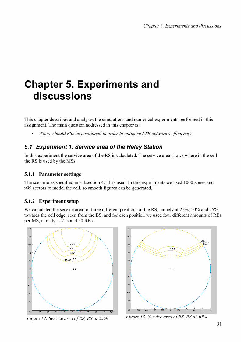
5.1 Experiment 1. Service area of the Relay StationIn this experiment the service area of the RS is calculated. The service area shows where in the cell the RS is used by the MSs.

5.1.1 Parameter settingsThe scenario as specified in subsection 4.1.1 is used. In this experiments we used 1000 zones and 999 sectors to model the cell, so smooth figures can be generated.

5.1.2 Experiment setupWe calculated the service area for three different positions of the RS, namely at 25%, 50% and 75% towards the cell edge, seen from the BS, and for each position we used four different amounts of RBs per MS, namely 1, 2, 5 and 50 RBs.

31Figure 12: Service area of RS, RS at 25% Figure 13: Service area of RS, RS at 50%

5.1 Experiment 1. Service area of the Relay Station

5.1.3 MethodThe service area is calculated by calculating the data rate for each possible MS position, given the RS position and the amount of RBs. After that the area where using the RS achieves a higher data rate is shown.

5.1.4 ResultsThe results are presented in Figure 12, Figure 13 and Figure 14, which show the service area of RS, when the RS is located at 25%, 50% and 75%, respectively, towards the radio cell edge, seen from the BS.

5.1.5 DiscussionThe first observation that can be made from the figures the usage of more RBs by the MS leads to a bigger service area for the RS. This is not as trivial as it might look, so an explanation will follow. First, notice that the effect of using more RBs really is that there is less power that can be used per RB. So Shannon's formula for the data rate can be considered to see the effect of less power per RB:

C=BW log2(1+S (r )N ) [bits per second] (24)

with (using Equation 4)

S r =P rx r =⋅Ptx

r a (25)

where ε is a certain constant.

Because the effect of the change of position on the data rate per RB has to be found, we will derive this formula with respect to r:

32

Figure 14: Service area of RS, RS at 75%


dCdr

= −BW

(1+ϵPtx

ra N )ln(2)⋅ϵ Ptx

ra+1 (26)

Now for interesting values of r, with the given parameter-settings, the following holds:

ϵ P tx

ra N≫1 (27)

Which means that the change in data rate per RB is almost independent of Ptx! So it does not matter if the data rate per RB at a certain point is 140 kbit/s (e.g. 1RB) or 80 kbit/s (e.g. 2RBs), if the distance dr from or to the BS or RS is varied, the same difference in data rate can be observed. On the other hand, using the RS results in half the effective data rate than using the BS. This is absolutely seen a much higher price to pay compared to changing dr if the data rate per RB is high, so the service area of the RS will be smaller when the data rate per RB is high. As few RBs assigned gives a higher the data rate per RB than many RBs assigned, the service area of the RS will be bigger when there are many RBs assigned.

Let's take a very simple example where we have a cell-set-up with an MS, a BS, and an RS 1km from it the BS. Assume the MS can achieve data rates to the BS of 140 kbit/s with 1RB and 80 kbit/s with 2RBs. The same MS can than of course achieve data rates to the RS of 70 kbit/s with 1RB and 40 kbit/s with 2RBs. The 'gap' between maximum BS and maximum RS speed is 60 kbit/s in the 1RB

case, but only 30 kbit/s in the 2RBs case. Assuming a dCdr of -10 kbit/s/100m for moving away

from the MS and -5 kbit/s/100m for moving away from the RS in both cases, we can very easily conclude that the position where the switch will take place is much closer to the RS for the 1RB case than for the 2RBs case (supposing r=0 at the BS).

For 1RB:

140−10r=70−5(10−r)r=8=800m (28)

For 2RBs:

80−10r=40−5(10−r )r=6=600m (29)

Note that the radius dependency of dCdr is not considered in the above equation. Including it will

make the speed loss bigger close the the concerning station, and less severe further from it.

The second observation that can be made is the unexpected cove around the RS when high transmitting power is used. The explanation for this is simple and is an caused by the maximum MCS (Modulating and Coding Scheme) specified in the LTE technical reports. This causes a maximum data rate that can achieved. Because the UE has high transmitting power, the BS can be reached with a data rate higher than the RS can possibly achieve, because the RS cuts the effective data rate in half. This looks like an arc, because the data rate to the BS is the same at the same distance to the BS, which gives a circle. Just outside this arc, the acquired data rate is half of the global maximum data rate, because there the RS is being used and can be reached with a maximum data rate.

33

5.1 Experiment 1. Service area of the Relay Station

Please also note that a bigger service area does not necessarily has to mean a greater effect of the RS on total cell throughput or average mean file transfer time over the cell. This can be observed by comparing Figure 13 and Figure 14 to Figure 15 and is further discussed in subsection 5.2.5.

5.2 Experiment 2. Total uplink throughput and impact on cell capacityAnother interesting characteristic to investigate is the impact of RS on the maximum arrival rate. When incorporating an RS, the total throughput to the BS should be higher, and so a higher arrival rate of users should be possible before the system becomes unstable. It is important to note that when users arrive at a faster rate than the system can serve them, the system becomes to be unstable.

5.2.1 Parameter settingsHere we also use the scenario as specified in subsection 4.1.1 is used, but with less zones and sectors, respectively 500 and 499. We will not generate a cell figure for this experiment, and less zones and sectors provide faster simulation without losing much accuracy.

5.2.2 Experiment setupThe performance measures that are investigated in this experiment are the total uplink throughput and the capacity of the system described in subsection 4.1.2. The experiment was done for each λ value from 4 to 7, with steps of 0.5 λ and for the scenario without RS, and with RS placed at 25%, 50%, 75% and 100%.

5.2.3 MethodThe simulation is run as explained in subsection 4.2.5. When the simulation is finished, the total data transmitted is divided by the total run time to get the total data throughput. There is a time needed to fill up the queue, so the first few seconds of the simulation are disregarded to get steady state plots faster. Also, the experiments were run three times in order to check the accuracy. First, the average of the three runs is plotted, and then the 95% confidence intervals are calculated and plotted by using the t-distribution.

5.2.4 ResultsThe results are presented in Figure 15. It can be seen that the errors on simulation results are quite small, so enough time was simulated. To clarify the figure, 'Without RS' and 'RS at 25%' have reached maximum capacity at ~5.3Mbps, 'RS at 50%' and 'RS at 100%' reach maximum capacity at ~5.7Mbps and with 'RS at 75%' the capacity rises to ~5.8Mbps.

5.2.5 DiscussionAs can be seen in Figure 15, the total throughput of the system can rise by about 10% when an RS is incorporated. This might look like a small increase, but the contribution to the total throughput is mainly from users nearby the BS, who have superior data rates. Also, only a small part of the remote users receive a speed boost, as can be seen in Figure 12, Figure 13 and Figure 14. Although it may not be the case that the total throughput rises much, for some users the increase in throughput is tremendous, as can be derived e.g. from Figure 17.Another observation that can be made is that the total throughput seems independent of the RS as long as maximum capacity is not reached. This is of course pretty logical. As long as the maximum capacity is not reached, all the users will eventually get served. So the average total throughput equals average arrival rate * average file size, independent of the RS.

34


A different way to describe this is by the fact that as the average data rate gets higher (for example because of the addition of an RS), the amount of users busy uploading at a given time gets lower: 10 MSs consecutively uploading with 1 Mbit/s has the same total throughput as 100 MSs uploading in parallel with 0.1 Mbit/s.

As soon as the average arrival rate gets near maximum capacity, then it does matter how fast the data rate per MS is. For as the data rate per MS increases, an MS finishes transmitting its file faster, and new users can be helped at a faster rate, which increases maximum capacity. So the maximum capacity will increase with a higher average data rate.

It can also be observed that the RS at 75% has the highest total uplink throughput, as can be seen in Figure 15, while its service area is not the largest, compare Figure 13 and Figure 14. The reason

35

Figure 15: Total uplink throughput

4 4,5 5 5,5 6 6,5 73,5

4

4,5

5

5,5

6

Without RS

RS at 25%RS at 50%

RS at 75%

RS at 100%

Arrival rate (λ) [in avg. arrivals/sec]

Tota

l upl

ink

thro

ughp

ut [i

n M

bit/s

]

5.2 Experiment 2. Total uplink throughput and impact on cell capacity

therefore is twofold: (1) the mean file transfer time of the MSs helped is relatively increased more because the RS is now closer to the MSs that had the poorest performance and (2) the most remote MSs are the bottleneck of the system; they keep the RBs busy for the local MSs which can make better use of them, so helping the poorest performing MSs will also help good performing MSs.

Correlation between maximum total uplink throughput and system capacityFor resource-fair schedulers, we can state that the arrival rate at which maximal throughput is reached, is equal to the maximal arrival rate of the system, in other words the system capacity. This can be proven as follows. As long as the total throughput rises, it means that the system could be used more efficiently. The only way for a resource-fair system to be more efficient, is when an MS is scheduled more than 1 RB once in a while, which is only possible if there are less MS uploading then there are RBs available, so we can conclude that the system is stable.

For unfair schedulers, for example the MAV scheduler, which assigns RBs to the MS who can achieve the highest data rate with it, this is not the case, because when using the MAV scheduler the total throughput also increases by scheduling MSs closer to the BS. In fact, the more MSs there are in the system, the more MSs will be located near the BS. So the MAV scheduler will only reach its maximum uplink throughput when the arrival rate is so high that it can constantly serve only MSs in the first zone, closest to the BS. To always have so many MSs close to the BS, the arrival rate must be very high. This is far beyond the system capacity, as all other MSs outside this zone will never be served at all.

5.3 Experiment 3. Impact of RS position on mean file transfer time per segment

5.3.1 Parameter settingsThe network scenario specified in subsection 4.1.1 is again used, but with even less zones and sectors than in Experiment 2, i.e. 50 zones and 49 sectors, since many MSs need to arrive in a segment to get meaningful averages values of the observed performance measure.

5.3.2 Experiment setupThe experiment was done for each λ value from 1 to 6, with a stepsize of 1 λ and for the scenario's with RS placed at 25%, 50%, 75% and 100% towards the radio cell edge, seen from the BS. The performance measure that is investigated in this experiment is the mean file transfer time described in subsection 4.1.2.

5.3.3 MethodThe simulation is performed as explained in subsection 4.2.5. The total upload time and the total amount of complete files transmitted is kept track off. When the simulation is finished, the total total upload time is divided by the amount of files transmitted to get the mean file transfer time per segment. Again the first few seconds of the simulation are disregarded to get steady state plots faster, see subsection 5.2.3. We kept the amount of segments low, because we need lots of files transmitted per segment, as the mean file transfer time can differ pretty much per file, as it depends strongly on the amount of RBs assigned.

5.3.4 ResultsThe results are presented in Figure 16, Figure 17, Figure 18 and Figure 19, for respectively the RS at 25%, 50%, 75% and 100% near the cell edge.36


Figure 16: Mean file transfer time, RS at 25% near cell edge

37



38



39


Figure 19: Mean file transfer time, RS at the cell edge

40


5.3.5 DiscussionThe most noticeable obtained results are probably the Figures 16(f), 17(f), 18(f) and 19(f). What can be seen here are unstable systems; MSs arrive faster than can be served, so the mean file transfer time goes to infinite. Because only a certain time is simulated, the mean file transfer times will not be infinite, but just very high, notice the different scales used on these figures.

What the figures show really well is the impact of the RS on the mean file transfer times for MSs located at different segments. The mean file transfer time has lowered very much around the RS. The RS covers about a quarter of the cell, so it seems that three more RSs could be added to increase the effects.

What can also be seen is that, although according to Experiment 1 the RS at 25% near cell edge has a reasonable service area, Figure 16 shows that that does not have to mean a substantial effect on the mean file transfer times. Because the RS is so close to the BS, the effects of the RS are marginal.

Furthermore, comparing Figures 16(e), 17(e), 18(e) and 19(e), it can be seen that with λ =5 and the RS located at 25% near the cell edge, the mean file transfer times are pretty high already: the system is almost unstable. With the RS located at 50% and at 100% the system is performing better. When the RS is located at 75% towards the cell edge, than the average mean file transfer time over the cell is the best, which can also be deducted from Figure 15.

41

Chapter 6. Conclusion and future work


The questions derived in Chapter 1 of this study were:

1. How does LTE operate, in particular the uplink resource management related to our study?2. What are the assumptions and requirements on the uplink imposed by the RS?3. Which performance models can be used to analyse the effect an RS on the performance of

MSs, giving the position of the RS and the MS in the network?4. Where should RSs be positioned in order to optimise LTE network's efficiency?

With regard to the first question, we can say that LTE consist of two parts, the core network and the radio access network, where the access network is in control of the air interface, so controls the uplink resources. The air resources are split into RBs, which are schedules by the eNode-B.

An important answer to the second research question is related to the fact that the usage of RS imposes restrictions on the usage of the resource blocks, as the MS that uses the RS can only transmit on half of the RBs assigned for it, as the other half is needed for the communication between the RS and the BS.

On behalf of the third question, we have developed a Matlab model which splits the cell into multiple segments, each with equal size, which are addressed by a zone and sector coordinate. Using this model of the cell, we can easily simulate the dynamic behaviour of users within the cell. For calculating the data rate of the MSs a path loss model and Shannon's theorem for maximum data rate was used.

In order to answer the fourth question, several performance experiments have been conducted. First the service area of the RS has been investigated, using different positions of the RS and different amount of RBs available to the MS. It was observed that the RS located at 75% towards the cell edge, has the smallest service area, but we concluded that this does not have to mean that it is performing the worst.

Hereafter we investigated the total uplink throughput and system capacity. It was shown that the RS placed at 75% towards the cell edge has the highest total uplink throughput, and therefore also has the highest system capacity. This was further shown in the last experiment, where the mean file transfer time for each segment for different arrival rates and RS positions was investigated.

So it can be concluded that the best place to locate an RS is at 75% near cell edge , assuming that (1) only a single radio cell is used, (2) no interference from other cells is considered, (3) the FWC scheduler is used.

43


Future study should be done to investigate the effect of (1) incorporating multiple RSs into the cell, (2) take interference from other cells into account, (3) using other types of schedulers. Letting RSs reuse frequencies from the BS it could be interesting too, but much care should be taken with regard to interference then.

Another issue that can be investigated is the impact of a dynamic back-haul link on the MS uplink performance. In this assignment, this link is modelled in such a way that the RS uses the same data rate for its communication to the BS as the MS did for the communication with the RS, which is not optimal.

44

Chapter 7. References


[3GPP11] 3GPP; , “3GPP TR 36.942 – Version 10.2.0; Technical Specification Group Radio Access Network; Evolved Universal Terrestrial Radio Access (E-UTRA); Radio Frequency (RF) system scenarios (Release 10),” Technical specifications from 3GPP, Annex A, 2011

[3GPP10] 3GPP; , “3GPP TR 36.814 – Version 2.0.0; Technical Specification Group Radio Access Network; Further Advancements for E-UTRA Physical Layer Aspects (Release 9),” Technical specifications from 3GPP, Chapter 9, 2010

[ChJe09] Byungjin Chun; Eui-Rim Jeong; Jingon Joung; Yukyung Oh; Yong H. Lee; , "Pre-nulling for self-interference suppression in full-duplex relays," Asia- Pacific Signal and Information Processing Association Annual Summit Conference (APSIPA ASC), Oct. 2009

[Cina10] Çinar, M.; , “Implementation of relay-based systems in wireless cellular networks,” M. Sc. Thesis, Izmir Institute of Technology, August 2010

[DaPa11] Dahlman, E.; Parkvall, S.; Sköld, J.; , “4G: LTE/LTE-Advanced for Mobile Broadband”, Academic Press, 26 apr. 2011

[DiBe10] Dimitrova, D.C.; Berg, H. van den; Litjens, R.; Heijenk, G.; , “Scheduling Strategies for LTE Uplink with Flow Behaviour Analysis”, Proc. of 4th ERCIM Workshop on eMobility, pp. 15 – 27, 2010

[Dimi10] Dimitrova, D.C.; “Analysing uplink scheduling in mobile networks; A flow-level perspective,” Ph. D. Thesis, University of Twente, November 2010

[Econ10] E-consultancy.com; , “Study: Mobile internet traffic is set to grow 400% by 2015,” downloaded from http://econsultancy.com/uk/blog/5683-study-mobile-internet-traffic-is-set-to-grow-400-by-2015, website of E-consultancy.com Limited, 2010, visited on 8 December 2011

[Expl08] Explanotech, Inc; , downloaded from http://3g4g.blogspot.com/2008/12/simplifying-ltesae-interfaces.html, 2008, visited on 30 January 2012

[Gess08] C. Gessner; , “UMTS Long Term Evolution (LTE) Technology Introduction , Application Note 1MA111 ,” downloaded from http://www2.rohde-schwarz.com/file_10948/1MA111_2E.pdf , website of Rohde & Schwarz, 2008, visited on 19 Jan. 2012

45


[HaWa10] Jing Han; Haiming Wang; , "Uplink Performance Evaluation of Wireless Self-Backhauling Relay in LTE-Advanced," 6th International Conference on Wireless Communications Networking and Mobile Computing (WiCOM), pp.1-4, 23-25 Sept. 2010

[HoHa11] Wei Hong; Jing Han; Haiming Wang; , "UL Performance Evaluation of Relay Enhanced FDD LTE-Advanced Networks," 7th International Conference on Wireless Communications, Networking and Mobile Computing (WiCOM), pp.1-5, 23-25 Sept. 2011

[HoKi11] Hossain, E.; Kim, Dong In; Bhargava, V.K.; , “Cooperative Cellular Wireless Networks,” Cambridge University Press, pp. 488, 2011

[HoTo10] Holman, H.; Toskala, A.; , “WCDMA for UMTS – HSPA Evolution and LTE, 5th ed.,” John Wiley & Sons Ltd., 2010

[KaBu10] Karaer, A.; Bulakci, O.; Redana, S.; Raaf, B.; Hamalainen, J.; , "Uplink performance optimization in relay enhanced LTE-Advanced networks," IEEE 20th International Symposium on Personal, Indoor and Mobile Radio Communications, pp.360-364, 13-16 Sept. 2009

[LePe09] Lee, S.B.; Pefkianakis, I.; Meyerson, A.; Xu, S.; Lu, S.; , "Proportional fair frequency-domain packet scheduling for 3GPP LTE uplink," Proceedings of the IEEE Conference on Computer Communications (INFOCOM '09), pp. 2611-2615, April 2009.

[MoWe07] Mogensen, P.; Wei Na; Kovacs, I.Z.; Frederiksen, F.; Pokhariyal, A.; Pedersen, K.I.; Kolding, T.; Hugl, K.; Kuusela, M.; , "LTE Capacity Compared to the Shannon Bound," IEEE 65th Vehicular Technology Conference, pp.1234-1238, 22-25 April 2007

[OPTA11] OPTA; , “Marktcijfers tweede kwartaal 2011,” downloaded from http://www.opta.nl/nl/actueel/alle-publicaties/publicatie/?id=3495 , website of OPTA, 2011, visited on 7 December 2011

[RaRe09] Rasheed, A.A.; Redana, S.; Raaf, B.; Hamalainen, J.; , "Uplink resource partitioning in relay enhanced LTE-Advanced networks," IEEE 20th International Symposium on Personal, Indoor and Mobile Radio Communications, pp.1502-1506, 13-16 Sept. 2009

[Roch99] University of Rochester; , “Lecture notes Astronomy 203/403, Fall 1999”, downloaded from http://www.pas.rochester.edu/~dmw/ast203/Lectures/Lect_20.pdf, website of University of Rochester, 1999, visited on 24 Jan. 2012

[Rumn08] Rumney, M.; , “3GPP LTE: Introducing Single-Carrier FDMA,” Agilent Technologies journal, 1 January 2008, downloaded from http://cp.literature.agilent.com/litweb/pdf/5989-8139EN.pdf, visited on 11 January 2011

[Saut10] Sauter, M.; , “From GSM to LTE,” John Wiley & Sons Ltd., 2010

[Shan48] Shannon, C.E.; , "A mathematical theory of communication," Bell System Technical Journal, Vol. 27, pp. 379–423, 623–656, July, October, 1948 : 10.1109/PIMRC.2009.5449788

[Wand11] Wanda, A.; , “The Notion of Radio Resource in LTE”, downloaded from http://trends-in-telecoms.blogspot.com/2011/05/notion-of-radio-resource-in-lte.html, 2011, visited on 30 January 2012

46

Appendix A. Matlab code


experiment1_25.m: %relay_position=[62,number_of_sectors/2+0.5]; % relay on 25% figure hold on contour(squeeze(circlematrix(1,:,:)), 'DisplayName', 'circlematrix', 'YDataSource', 'circlematrix'); contour(squeeze(circlematrix(2,:,:)), 'DisplayName', 'circlematrix', 'YDataSource', 'circlematrix'); contour(squeeze(circlematrix(5,:,:)), 'DisplayName', 'circlematrix', 'YDataSource', 'circlematrix'); contour(squeeze(circlematrix(50,:,:)), 'DisplayName', 'circlematrix', 'YDataSource', 'circlematrix'); plot(500,625) set(gca,'DataAspectRatio',[1 1 1],... 'PlotBoxAspectRatio',[1 1 1],'ZLim',[-0.6 0.6])

experiment1_50.m: %relay_position=[number_of_zones/4,number_of_sectors/2+0.5]; % relay on 50% figure hold on contour(squeeze(circlematrix(1,:,:)), 'DisplayName', 'circlematrix', 'YDataSource', 'circlematrix'); contour(squeeze(circlematrix(2,:,:)), 'DisplayName', 'circlematrix', 'YDataSource', 'circlematrix'); contour(squeeze(circlematrix(5,:,:)), 'DisplayName', 'circlematrix', 'YDataSource', 'circlematrix'); contour(squeeze(circlematrix(50,:,:)), 'DisplayName', 'circlematrix', 'YDataSource', 'circlematrix'); plot(500,750) set(gca,'DataAspectRatio',[1 1 1],... 'PlotBoxAspectRatio',[1 1 1],'ZLim',[-0.6 0.6])

experiment1_75.m: %relay_position=[563,number_of_sectors/2+0.5]; % relay on 75% figure hold on contour(squeeze(circlematrix(1,:,:)), 'DisplayName', 'circlematrix', 'YDataSource', 'circlematrix'); contour(squeeze(circlematrix(2,:,:)), 'DisplayName', 'circlematrix', 'YDataSource', 'circlematrix'); contour(squeeze(circlematrix(5,:,:)), 'DisplayName', 'circlematrix', 'YDataSource', 'circlematrix'); contour(squeeze(circlematrix(50,:,:)), 'DisplayName', 'circlematrix', 'YDataSource', 'circlematrix'); plot(500,875) set(gca,'DataAspectRatio',[1 1 1],... 'PlotBoxAspectRatio',[1 1 1],'ZLim',[-0.6 0.6])

experiment2_core1.m:

clear; settings; use_a_relay=0; exp4=1; save exp4_settings.mat; zonecell_with_FWC_relay results_zonder=results; save results4.mat results_zonder;

clear; settings; use_a_relay=1; relay_position=[31,number_of_sectors/2+0.5]; exp4=1; save exp4_settings.mat; zonecell_with_FWC_relay results_25=results; save results4.mat results_25 -APPEND;

47


experiment2_core2.m:

%should be started after core 1, because of the -append clear; settings; use_a_relay=1; relay_position=[125,number_of_sectors/2+0.5]; exp4=1; save exp4_settings.mat; zonecell_with_FWC_relay results_50=results; save results4.mat results_50 -APPEND;



experiment3.m:

clear; settings; use_a_relay=0; exp5=1; save exp5_settings.mat; zonecell_with_FWC_relay results_zonder=results; save results5.mat results_zonder;




clear; settings; 48


use_a_relay=1; relay_position=[50,number_of_sectors/2+0.5]; exp5=1; save exp5_settings.mat; zonecell_with_FWC_relay results_100=results; save results5.mat results_100 -APPEND;

MaakMooieCirkel_exp3:

radiuspoints=500;

circlematrix=zeros(2*radiuspoints,2*radiuspoints);

sizex=size(circlematrix,1); sizey=size(circlematrix,2);

meantime_without=results_zonder(:,:,1)./results_zonder(:,:,2); meantime_25=results_25(:,:,:,1)./results_25(:,:,:,2); meantime_50=results_50(:,:,:,1)./results_50(:,:,:,2); meantime_75=results_75(:,:,:,1)./results_75(:,:,:,2); meantime_100=results_100(:,:,:,1)./results_100(:,:,:,2); finito_without=[]; finito_with=zeros(4,8,50,49); %without interpol %finito_with=zeros(4,8,197,193); %with interpol circlematrix_with=zeros(4,8,size(circlematrix,1),size(circlematrix,2)); for x=1:8 % finito_without=interp(squeeze(meantime_without(x,:)),2); % finito_with(1,x,:,:)=interp2(squeeze(meantime_25(x,:,:)),2); % finito_with(2,x,:,:)=interp2(squeeze(meantime_50(x,:,:)),2); % finito_with(3,x,:,:)=interp2(squeeze(meantime_75(x,:,:)),2); % finito_with(4,x,:,:)=interp2(squeeze(meantime_100(x,:,:)),2); finito_without=squeeze(meantime_without(x,:)); finito_with(1,x,:,:)=squeeze(meantime_25(x,:,:)); finito_with(2,x,:,:)=squeeze(meantime_50(x,:,:)); finito_with(3,x,:,:)=squeeze(meantime_75(x,:,:)); finito_with(4,x,:,:)=squeeze(meantime_100(x,:,:)); end

finito_with(:,:,:,size(finito_with,4)+1)=finito_with(:,:,:,1);

for pos=1:4 for lab=1:8 finito=squeeze(finito_with(pos,lab,:,:)); number_of_zones=size(finito,1); number_of_sectors=size(finito,2)-1; zones_radii=DetermineZonesRadii(cell_radius,number_of_zones); for x=1:sizex for y=1:sizey magnitude=sqrt( (x-sizex/2)^2+(y-sizey/2)^2 ); if magnitude/radiuspoints>1 circlematrix(y,x)=0; else if x==sizex/2 if y>sizey/2 angle=pi/2; else % so also if y=sizey/2 angle=-pi/2; end else angle=atan( (y-sizey/2)/(x-sizex/2) ); end angle=angle+pi/2; if x<sizex/2 angle=angle+pi; end thezone=1; while (magnitude>zones_radii(thezone)/(cell_radius/radiuspoints)&&thezone<number_of_zones) %zones_radii(max) is a tiny fraction smaller then cell_size because of algoritm, so we need the extra check thezone=thezone+1; end

49


thesector=floor(angle/(2*pi)*number_of_sectors)+1; circlematrix(y,x)=finito(thezone,thesector);

end end end for x=-5:5 for y=-5:5 circlematrix(sizey/2+y,sizex/2+x)=20; if pos==1 circlematrix(5*sizey/8+y,sizex/2+x)=20; elseif pos==2 circlematrix(6*sizey/8+y,sizex/2+x)=20; elseif pos==3 circlematrix(7*sizey/8+y,sizex/2+x)=20; elseif pos==4 circlematrix(8*sizey/8+y-5,sizex/2+x)=20; end end end circlematrix_with(pos,lab,:,:)=circlematrix; end end

PlotMooieCirkel_exp3.m:

postext={ '25%', '50%', '75%' ,'100%' }; for pos=1:4 for lamb=1:8 prooi=squeeze(circlematrix_with(pos,lamb,:,:)); figure; handle=imagesc(prooi); title(['\fontsize{12}\bfMean file transfer time, RS at ',char(postext(pos)),', lambda=',num2str(lamb)]); xlabel('\bfCell range [km]'); ylabel('\bfCell range [km]'); set(gca,'XTick',0:250:1000); set(gca,'XTickLabel',{'1','0.5','0','0.5','1'}); set(gca,'YTick',0:250:1000); set(gca,'YTickLabel',{'1','0.5','0','0.5','1'}); h=colorbar; ylabel(h,'\bfMean file transfer time [s]'); geenprocent=char(postext(pos)); if pos==4 text=geenprocent(1:3); else text=geenprocent(1:2); end saveas(handle,['exp5_interpol_',text,'_',num2str(lamb),'.png']); delete(handle); end end

zonecell_with_FWC_relay.m:

reset=1;

if ~exist('reset','var') reset=1; end

if reset==1 if exist('exp4','var') clear; reset=0; load exp4_settings.mat; elseif exist('exp5','var') clear; reset=0; load exp5_settings.mat; else clear; reset=0; %Set the parameters settings; 50


use_a_relay=1; end %%%%Determine the radii with equal surface in the rings between the radii zones_radii=DetermineZonesRadii(cell_radius,number_of_zones); %%%%Determine the distance between a sector and the relay distance_to_relay=DetermineDistanceToRelay(zones_radii,number_of_sectors,relay_position); datarate_of_zones_sectors; datarate_of_zones; else settings; end

t_start=cputime;

% 1=datarate calculation 2=circle generation todo=1;

switch todo case 1, lambda_start=1; lambda_step=1; lambda_end=8; avgqueue=0; for lambda=lambda_start:lambda_step:lambda_end for confidence=1:5 queue=[]; gross_totaldatatransmitted=0; net_totaldatatransmitted=0; totalwaittime=0; ppl_helped=0; idletime=0; avgdaterate=0; if use_a_relay==1 finishe_d=zeros(number_of_zones,number_of_sectors,2); else finishe_d=zeros(number_of_zones,2); end settletime=(1/lambda)*100; % we are settled when on average 100 requests have been made, because the maximum possible average speed is obtained with 50 mobiles in the queue. if exist('exp5','var') time_simulated=fix(75000/lambda); % we want to have enough people helped per segment, so we can have confident mean file transfer ratio's %time_simulated=100 end for iteration=1:time_simulated/timestep if (rand<(lambda*timestep)) if use_a_relay==1 queue(end+1,1:4)=[filesize unidrnd(number_of_zones) unidrnd(number_of_sectors) iteration]; else queue(end+1,1:3)=[filesize unidrnd(number_of_zones) iteration*timestep]; end end avgRB=totalRBs/min(size(queue,1),50); if size(queue,1)==0 && (iteration>settletime/timestep) idletime=idletime+timestep; else for x=1:min(size(queue,1),50) if avgRB==fix(avgRB) if use_a_relay==1 datarateprime=relay_real_datarate(queue(x,2),queue(x,3),avgRB); else datarateprime=datarate(queue(x,2),avgRB); end else highRB=ceil(avgRB); lowRB=floor(avgRB);

51


if use_a_relay==1 datarateprime= (highRB-avgRB)*relay_real_datarate(queue(x,2),queue(x,3),lowRB)+(avgRB-lowRB)*relay_real_datarate(queue(x,2),queue(x,3),highRB); else datarateprime= (highRB-avgRB)*datarate(queue(x,2),lowRB)+(avgRB-lowRB)*datarate(queue(x,2),highRB); end end queue(x,1)=queue(x,1)-timestep*datarateprime; if queue(x,1)<=0 if use_a_relay==1 finishe_d(queue(x,2),queue(x,3),1:2)=[finishe_d(queue(x,2),queue(x,3),1)+(iteration-queue(x,4))*timestep finishe_d(queue(x,2),queue(x,3),2)+1]; else finishe_d(queue(x,2),1:2)=[finishe_d(queue(x,2),1)+(iteration-queue(x,3))*timestep finishe_d(queue(x,2),2)+1]; end end

if (iteration>settletime/timestep) avgqueue=avgqueue+1; gross_totaldatatransmitted=gross_totaldatatransmitted+timestep*datarateprime; net_totaldatatransmitted=net_totaldatatransmitted+timestep*datarateprime+min(0,queue(x,1)); totalwaittime=totalwaittime+timestep; %data_zone_sector_wait(zone,sector,:,:)=data_zone_sector_wait(zone,sector,:,:)+[ timestep*datarateprime, timestep ]; end end end if (iteration>settletime/timestep) %for x=sizequeue+1:min(size(queue,1),50) avgqueue=avgqueue+max(0,size(queue,1)-50)*timestep; totalwaittime=totalwaittime+max(0,size(queue,1)-50)*timestep; %data_zone_sector_wait(zone,sector,:,:)=data_zone_sector_wait(zone,sector,:,:)+[ timestep*datarateprime, timestep ]; %end end

ppl_helped=ppl_helped+size(queue,1)-sum(all(queue>0,2)); queue=queue(all(queue>0,2),:);

end lambda size(queue,1) ppl_helped ShowSpeed t_used=cputime-t_start if exist('exp4','var') results(confidence,lambda)=net_averagespeed; elseif exist('exp5','var') if use_a_relay==1 results(lambda,:,:,:)=finishe_d; else results(lambda,:,:)=finishe_d; end end end end case 2, radiuspoints=500; forRBs = [1 2 5 10 20 50]; circlematrix=zeros(50,2*radiuspoints,2*radiuspoints); sizex=size(circlematrix,2); sizey=size(circlematrix,3); use_relay(:,number_of_sectors+1,:)=use_relay(:,1,:); for z=forRBs for x=1:sizex for y=1:sizey magnitude=sqrt( (x-sizex/2)^2+(y-sizey/2)^2 ); 52


if magnitude/radiuspoints>1 circlematrix(z,y,x)=-111; else if x==sizex/2 if y>sizey/2 angle=pi/2; else % so also if y=sizey/2 angle=-pi/2; end else angle=atan( (y-sizey/2)/(x-sizex/2) ); end angle=angle+pi/2; if x<sizex/2 angle=angle+pi; end thezone=1; while (magnitude>zones_radii(thezone)/(cell_radius/radiuspoints)&&thezone<number_of_zones) %zones_radii(max) is a tiny fraction smaller then cell_size bacause of algorithm, so we need the extra check thezone=thezone+1; end thesector=round(angle/(2*pi)*number_of_sectors)+1; circlematrix(z,y,x)=111*use_relay(thezone,thesector,z); if (thezone==relay_position(1) && thesector==relay_position(2)) circlematrix(z,y,x)=222; x y end end end end circlematrix(z,sizey/2,sizex/2)=222; end end

DetermineZonesRadii.m:

function zones_radii = DetermineZonesRadii( my_cell_radius, my_number_of_zones )

surface_per_zone=pi*my_cell_radius^2/my_number_of_zones;

r(1)=0; for x=1:my_number_of_zones r(x+1)=sqrt(surface_per_zone/pi + r(x)^2); end

zones_radii=r(2:end);

DetermineDistanceToRelay.m:

function distance_to_relay = DetermineDistanceToRelay( myzonesradii, mysectors, myrelaypos )

myzones=numel(myzonesradii); for x=1:myzones for y=1:mysectors r1=myzonesradii(myrelaypos(1)); r2=myzonesradii(x); angle=2*pi/mysectors*(myrelaypos(2)-y); distance_to_relay(x,y)=sqrt(r1^2+r2^2-2*r1*r2*cos(angle)); %cosine rule % difff(x,y)=sign(zones_radii(x)-distance_to_relay(x,y)*2^(1/2.5))+1; end end

datarate_of_zones_sectors.m:

m=(1:totalRBs); m=m(ones(1,number_of_zones),:); zones_radii_relay=zones_radii(ones(1,totalRBs),:)'; % need multiple powerdivisions SNR_of_zones=(P_max./m) ./ (N.*L(zones_radii_relay./1000)); SNR_of_zones=min(SNR_of_zones,maxSNR); datarate_without_relay=m.*BW.*shannon_efficiency.*log2(1+SNR_of_zones);

%relayspeeds relay_instant_datarate(zone,sector,RBs) for x=(1:totalRBs) %powerdistance_to_relay=distance_to_relay./x

53


SNR_of_distance_to_relay = (P_max./x) ./ (N.*L(distance_to_relay./1000)); SNR_of_distance_to_relay = min(SNR_of_distance_to_relay,maxSNR); relay_instant_datarate(:,:,x) = x.*BW.*shannon_efficiency.*log2(1+SNR_of_distance_to_relay); end

relay_real_datarate=relay_instant_datarate./2;

for x=(1:number_of_sectors) %use_relay(zone,sector,RBs) use_relay(:,x,:)=squeeze(relay_real_datarate(:,x,:))>datarate_without_relay(:,:); relay_real_datarate(:,x,:)=max(squeeze(relay_real_datarate(:,x,:)),datarate_without_relay); end

datarate_of_zones.m:

m=(1:totalRBs); m=m(ones(1,number_of_zones),:); zones_radii=zones_radii(ones(1,totalRBs),:)'; % need multiple powerdivisions SNR_of_zones=(P_max./m) ./ (N.*L(zones_radii./1000)); SNR_of_zones=min(SNR_of_zones,maxSNR); datarate=m.*BW.*shannon_efficiency.*log2(1+SNR_of_zones);

ShowSpeed.m:

gross_averagespeed= gross_totaldatatransmitted/(time_simulated-settletime-idletime) net_averagespeed= net_totaldatatransmitted/(time_simulated-settletime-idletime) user_gross_averagespeed= gross_totaldatatransmitted/totalwaittime user_net_averagespeed= net_totaldatatransmitted/totalwaittime avgdatarate

L.m:

function [ my_path_loss ] = L( my_d ) %(COST) HATA 321 model %L Get the pathloss as function of distance % This function calculates the path loss as a function of the distance % Usage: pathloss = L(d) (d=distance in km)

PLfix=141.6; %PLfix=125.6; a=3.53; %a=1;

%in dB %my_path_loss=PLfix+10*a*log10(my_d)

%linear my_path_loss=10^(PLfix/10)*(my_d).^a; %my_path_loss=(my_d).^a

settings.m:

%% static

cell_radius=1000; % in meters number_of_zones=50; % different per experiment number_of_sectors=49; P_max=0.200; % in W N=10^((-121.45+5)/10)/1000; % -121.45dBm per subcarrier with noise figure of 5 dB shannon_efficiency=0.4; BW=180000; TTI=0.5e-3; %in sec totalRBs=50; maxSNR=10^1.5; relay_position=[number_of_zones/4,number_of_sectors/2+0.5]; % relay on .5*cell_radius[m] = number_of_zones/4 %depends on experiment, some experiments set in themselves totalwaittime=0;

%% dynamic

lambda=.1; %average arrivals/sec timestep=10e-3; time_simulated=5000; %in sec filesize=1e6; %in bits queue=[]; gross_totaldatatransmitted=0; net_totaldatatransmitted=0; ppl_helped=0; idletime=0; avgdatarate=0;54

Documents

Analysing uplink performance in relay-enabled LTE-networks · To catch up with this enormous rise in cellular traffic, ... Cellular network with relay. ... GSM/UMTS networks if the