Embed Size (px)
Citation preview

Purdue University Purdue University
Purdue e-Pubs Purdue e-Pubs
Department of Computer Science Technical Reports Department of Computer Science
1975
Analysis & Applications of the Delay Cycle for the M/M/c Analysis & Applications of the Delay Cycle for the M/M/c
Queueing System Queueing System
K. Omahen
V. Marathe
Report Number: 75-165
Omahen, K. and Marathe, V., "Analysis & Applications of the Delay Cycle for the M/M/c Queueing System" (1975). Department of Computer Science Technical Reports. Paper 111. https://docs.lib.purdue.edu/cstech/111
This document has been made available through Purdue e-Pubs, a service of the Purdue University Libraries. Please contact [email protected] for additional information.

· .
Analysis &Applications of the DelayCycle for the MIMIc Queueing System
K. OmahenDepartment of Computer Science
Purdue Universityw. Lafayette. IN 47907
~d
V. MaratheDepartment of Business Administration
University of IllinoisUrbana~ IL 61801
CSD-TR 165
Keywords: Delay Cycle Analysis, Busy Period Analysis.MIMIc Queueing System. Waiting Time Distributions.Multiprocessor Models.
-1-
1. IntroductionThis paper addresses the problem of solving mUltiple-serverqueueing models through the use of busy-period analyses. In thepast, this technique of busy-period analysis has been extensivelyused for the M/G/I queueing system and found to be a powerfultool for dealing with a great many complex scheduling rules. particularly those involving preemptive and nonpreemptive priorities.The results presented in this paper demonstrate that the methodof busy-period analysis can be extended to ~eal with certain instances of the MIMIc queueing system as well. In references (1,2),the authors independently made use of this general technique tosolve multiple-server.models for which jobs have simultaneousresource requirements; an overview of this work is contained inreference [3].
The method of analysis involving decomposition of busy periodswas first used by Cobham l4] and later by AVi-Itzhak, Maxwell, andMiller [5] and others; the text by Conway. Maxwell. and Miller [6]contains many of the results obtained for the M/G/l queueingsystem through the use of this technique. In order to motivatethe analysis to be presented, the typical sequence of steps in sucha busy-period analysis will be briefly covered.When the tern "busy-period" is used, we will be referring to aninterval during which one or more jobs are in service. There willgenerally be a number of different busy-periods for a system, andsystem states will be defined so as to include the idle state and anumber of mutually exclusive and exhaustive busy states correspondingto these different types of busy-periods. The system states aredefined so that the state transition process is Markovian, and thelimiting probability of the system being in a particular state maybe determined in a straightforward manner (e.g. using results fromthe theory of Semi-Markov processes [7]). The analysis typicallybegins by first finding the Laplace-Stieltjes Transform (LST) forthe distribution of busy period length for each case and thenobtaining the LST for the flow time or waiting time conditioned upon

-2-
the arrival finding a specified type of busy-period in progress.
If jobs are generated by means of a Poisson source~ the distribution
of system states at arrival epochs will be identical to the steady
state distribution of system states (see Strauch [8]). Using this
result. the unconditional LST for the distribution of flow time or
wa1t1ng time may be directly obtained. In principle, the LST
completely describes a distribution, but the inversion of the trans
form is usually so difficult as to require that a numerical transform
inversion software package be employed. In most cases the first two
moments of a random variable may be found from the LST withoutexcessive effort.
The system to be analyzed in this paper is the multiple-server
Poisson-Exponential queue, commonly denoted as the MIMic queueing
system. The model may be described as fallows:
There are c identical servers, each capable ofperforming one job at a time. The incoming jobshave independent and exponentially distributedprocessing reqUirements with mean l/~. The interarrival times are independent and exponentiallydistributed with mean l/A. It is assumed that theservers process the jobs continuously as long asthere are jobs in the system.
For each of the busy period types to be defined in later sections.
the LST and first two moments will be obtained. In addition, the..LST and first moment will be derived for the waiting time of a
job conditioned upon the arrival finding a specified busy-periodin progress.
2. Busy Periods for the MIMIc Queueing System
In a single-server system, a lInormalll busy period is usually
defined to be an interval which begins with the arrival of a job
to an empty system and which terminates when the system again
becomes idle; this busy period represents the length of time that
the (single) server is busy. A similar type of busy period for a
multiple-server system may be defined which is an interval during
which one or more processors are busy; however. there arc additional

-3-
busy periods which are of interest. Define the fOllowing typeof busy period for the MIMic queueing system:
Tk = min [t : (k) jobs in(k-l) n II
where integer k > 1.
system at time 0+]lr " time t
~(t) = Pr[Tk ~ t] = cumUlative distribution function (cdf) for Tk
,
nk(s) = LST for the distribution of Tko
The random variable (r.v.) may be considered as an interval during
which the number in system is greater than or equal to k; alternatively,
this variable represents the length of time necessary to achieve an
overall reduction of jobs in system by one. Due to the memoryless
property of the exponential processing times~ the distribution of
Tk will not depend on whether or not any of the k jobs have received
prior processing. For each random variable Tk
, we also define:
The properties of POisson processes summarized in Appendix 1 will
often be cited in the remainder of the paper, and the followingnotation will be employed:
A = (Poisson) arrival rate for jobs,
~ = (Exponential) processing rate for jobs,
~ = denotes 'distributed as' e.g. X~Y is interpreted to meanthat random variable X has the same distribution as r.v. Y.
Before proceeding into the analysis, a r.v. will be introduced whichsimplifies the presentation; for 1 ~ k ~ c, define:
Pk = r.v. denoting an interevent time associated with anaggregate of k simUltaneous Poisson processes, each with rate ~.
Gk(p) = cdf for Pk
,
yk(s) = LST for the distribution of Pk
.
Referring to Appendix 1. we easily find the following:
'k(s) = k./(s+k.J,
E(Pk) = l/(k.),
E(P~) = 2/(k.)2.
Given the above reSUlts, we may next analyze the properties of busyperiod T
k.
-4-
LEMMA 1. For the MIMIc queueing system. the distribution of
busy period Tk has the following characteristics:(i) For k > c.
Tk "'Te
(ii) For k = e,
n (5) = Y (s + A -An (5)),e e eE(T ) = E(Pe)/(1 -AE(Pe)],e
E(T2) = E(P~JlP -AE(Pe)]3.e
(iii) For 1 .::. k < c,
"k(5) ='Yk(5 + A -A"k+I(s)),
E(Tk ) = E(Pk) + AE(Pk)E(Tk
+I),
E(T~) = E(P~) [I+E(Tk+I)Y + AE(Pk)E(T~+I).Proof. We divide the proof into three sections corresponding tothe statement of the lemma.
(i) It is trivial to verify that, for k > C. T.V. Tk
has the
same distribution as T.V. T. There will be exactly c processorseactive throughout the duration of these busy periods, and these
busy periods also have identical arrival processes for jobs.
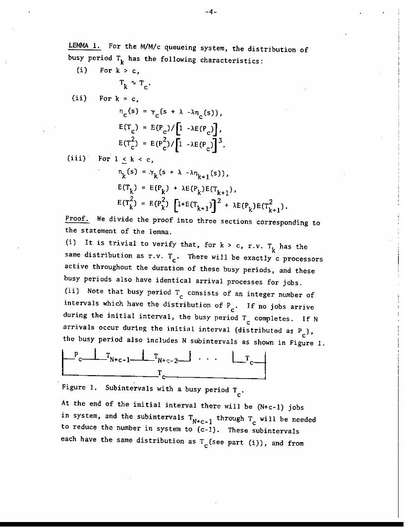
(ii) Note that busy period Tc consists of an integer number of
intervals which have the distribution of P. If no jobs arrivee
during the initial interval. the busy period T completes. If Ne
arrivals occur during the initilll interval (distributed as Pc)'
the husy period also includes N subintervals as shown in Figure 1.
Figure 1. Subintervals with a busy period T .e
in system,
to reduce
At the end of the initial interval there will be (N+c-l) jobs
and the subintervals TN 1 through T will be needed+c- cthe number in system to (e-l). These subintervals
eaeh have the same distribution as T (see part (i)), and frome
-5-
unconditional
the convolution property of the L5T we have
ne(sIPe=p,N=n) = exp(-SPl[ne(s)]n
Removing the conditioning on Nand P • thee
LST becomes
nets) = io (n~o ~AP)n/n~ eXp(-Ap) ne(s IPe=p,N=n)I= y (5 + A -An (5)).e e
dG (p),e
The properties of the LST allow the first two moments for Te
to be found from -TIl (0) and fi" (D) • respectively. Solving thee eresulting expressions for E(Te) and E(T~) gives the desired results.
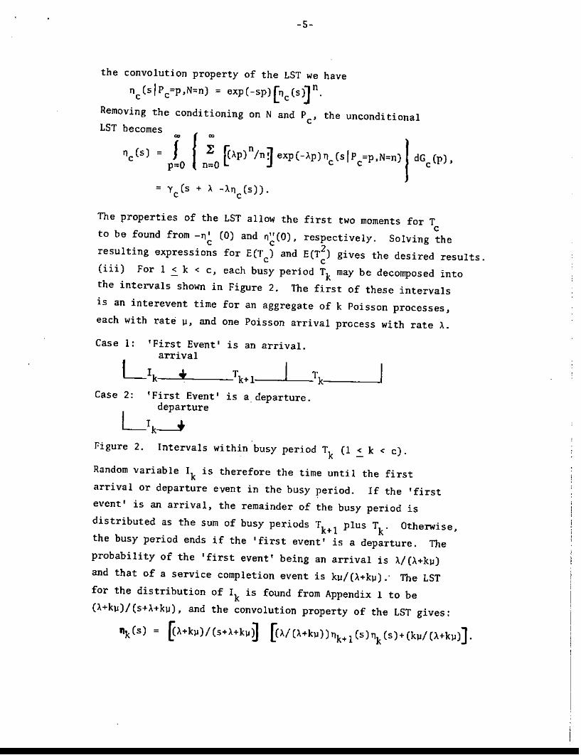
(iii) For 1 ~ k < c. each busy period Tk may be decomposed into
the intervals shown in Figure 2. The first of these intervals
is an interevent time for an aggregate of k Poisson processes,
each with rate ~. and one Poisson arrival precess with rate A.
Case 1: 'First Event' is an arrival.arrival
Llk + Tk+1-LTk: _
Case 2: 'First Event' is a departure.departure
Llk-----yfoigure 2. Intervals within busy period T
k(1 ~ k < c).
Random variable Ik is therefore the time until the first
arrival or departure event in the busy period. If the 'first
event' is an arrival, the remainder of the busy period is
distributed as the sum of busy periods Tk
+l
plus Tk
. Otherwise,
the busy period ends if the 'first event' is a departure. The
probability of the 'first event' being an arrival is h/(A+ku)
and that of a service completion event is kU/(A+kU)." The LST
for the distribution of Ik is found from Appendix 1 to be
(A+ku)/(S+A+ku), and the convolution property of the LST gives:
"k(s) = ~A+k")/(S+A+k"il [cA/(A+k"))nk+l(S)nk(s)+(k"/(A+k")].

-6-
Solving for nk(s), we obtain
nk (5) = k"!(k"+5+A-Ank+! (5)).
Noting that Yk(s) = k~/(k~+s). the above result may be written as
nk(5) = Yk(5 + A -Ank+!(5)).
The first two moments for Tk
are directly found by evaluating
-nk(O) and "keD), respectively. Q.E.D.
Another type of busy period found to be useful in the analysis
of the M/G/l system under non-preemeptive scheduling rules is the
delay cycle (cf. reference [6], Chapter 8). A delay cycle is a
generalized busy period which arises in situations where jobs
arrive while the processor is unavailable due to some reason; for
example. the processor(s) may be temporarily broken down or busy
servicing higher priority jobs. Figure 3 gives an example of a
delay cycle for the MIMIc queueing system.
system empty
systemempty
T:-....==:TD'--=:::;;;'-=:T~f~~:::;;'" ~===:T,-==:;:}"y- V ~delay c proces~ors busy time until
systemempty
Figure 3.
L----- Tee
_
Delay Cycle T for the MIMic queueing system.e
The delay TO represents an amount of time during which,.Tl c
processors are unavailable. At the conclusion of this delay, the
system will begin processing any jobs which arrived during the
initial interval. The remainder of the delay cycle is the sum of
two subintervals Tf and Tg during which jobs are serviced. Subinterval
Tf begins immediately after the delay and lasts until there are fewer
than c jobs in system (this subinterval has length zero if less than
c jobs arrive during the delay). Subinterval Tg
begins immediately
after Tf and represents the time necessary to clear the system of jobs.
The following notation is in~roduced to deal with the delay cycledescribed above:

-7-
TO = Delay during which the c processors are unavailable,HO(t) = cdf for TO'
nOes) = LST for the distribution of TO.
It is assumed that the LST and moments for r.v. TO are given.
cdf
[t:T = mine system empty at 0- ]delay interval TO commences at 0+system again empty at time t ~ TO
for Te
,
= LST for the distribution of T ;e
Tf = length of interval commencing immediately after delay TO
and terminating when there are less than c jobs in system,Hf(t) = cdf for T
f>
nf(s) = LST for the distribution of Tf
;
Tg = interval which begins at the conclusion of Tf
and whichlasts until the system is empty.
Hg(t) = cdf for Tg >
Tf • and Tg are given by:
ng(s) = LST for the distribution of Tg
We next present a lemma dC$cribing the distributions for therandom variables given above.
LEMMA 2. The LST and first moment for random variables T •e
c-l[no(S+A-Anc(S)) }] "j(S)] I Ec(S)]C-I
+ nO(s+A) p-{[~ nj (S)] I [nc(S~ C-I}]
+ ci/ 1(_I)nAn/n !1 nO(S+A){.fr n.(sUn n. (s)l/fnc(sll c-I-n]n=1 l' :J J=I J 'LJ=I J J L :J
cil
[(_I)nAn/n~ n~n) (A)n=O
c-I+InO(A-Anc(s))- n~o [(-l)nAn/njfc(S~nn6n)(A)}I[nc(sil c-I,

-8-
c-2 n+ 2: E-llnAn/ni'l"6nl(A) n ".(5)
n=l :J j=l)
"j (5l [1 :~: E-llnAn/n!]"~nl (Al],+c-ln
. j=1
= E(TOl + E(Tfl + E(Tgl,c-l
= E(TCl{ [AE(TOl - n;o [n(_llnAn/n~"6nl (Al]c-l
- (c-ll[l- n:o [c-llnAn/n~"6nl(A~},
c-l k-lk:l E(Tkl{1 - n:o E-llnAn/n~ "6
nl(Al}.E(T 1 =g
Proof. The above L5T5 are derived using similar techniques;
given the length of the delay and number of arrivals during
the delay, the conditional LST is found for each type of interval,
and the conditioning is then removed to find the final result.
Delay cycle Te consists of delay TO plus the time (sub
intervals Tf and Tg
) needed to clear the system of all jobs.
Recall that a busy period Tk (k ~ 1) represents the time
necessary to reduce the number of jobs in system from k jobs
to (k-l) jobs. If N jobs arrive during the delay TO' the
remainder of Te is the sum of busy periods TN through T1" It
follows that the conditional LST for the distribution of T equalse
exp (-5tl
exp (-stl
n
nj=1
"j (5l for n > O.
for n = O.
Since nj(s) = nc(s) for all j greater than c,
"e(5ITo=t,N=nl = exp(-5tl ["c(51 n-c+l
we have for nc-lIT ". (5l .j=1 J
> c
Removing the conditioning on the number of Poisson arrivals
during the delay and on the delay length, the unconditional
LST is found to be
"e(5) = JIi [CAtl"/n] exp (-At)"e(5!To=t,N=nl} dIlO(tl,t=O n=O

-9-
=
In obtaining this result, it was necessary to make use of the
following property of the Laplace-Stieltjes Transofrm (seereference [9] • p. 57):
t!a exp(-st)tndHa(t)
for c <: n.
n
n ". (s)j=l J
c-1n "j (5)j=l
The expression for ne(s) is, with minor rearrangement of terms.
the desired LST for the distribution of T .e
We next derive the LSTs for Tf
and Tg
• again conditioned
upon the number of arrivals during the delay and on the delny
length. Subinterval Tf has length zero if there are fewer than
c arrivals during delay TO; if there are N arrivals, where N
is greater than or equal to c, subinterval Tf
consists of the
sequence of busy periods TN' TN_1 •..••Tc
. Since each of these
busy periods has the same distribution as Te' the conditional
LST for the distribution of Tf becomes
-{I forO<n<c,[nc (s)]n-c+l for c <: n.
Subinterval Tg also has length zero if no jobs arrive during
the delay. If N jobs arrive during the delay. where N is some
positive integer less than c. subinterval Tg
is the sum of
busy periods Tn' TN_i, ...• Tl . Otherwise. Tg
begins immediately
after a subinterval Tf having length greater than zero. Since
subinterval Tf ends with (c-l) jobs in system, Tg
is the sum
of busy per~ods TC_1 through Tl . The conditional LST for the
distribution of Tg
is therefore given by
"g(SITa=t,N=n) = {I for n = a,
for 0 <: n ~ c-l.
\

-10-
The conditioning on nwnb ..· ~ of arrivals and on delay length for
the above can be removed:n exactly the same manner as used for
delay cycle T • and the d~sired LSTs are obtained .•The expected values f~l Te , Tfo and T
gfollow directly from
-n~(O), -Tlf(OL and -T]8~·O), respectively. Q.E.D.
At first glance. the telms appearing in the expressions forthe expected lengths of inte~vals Tf and T
gmay seem somewhat
PUzzling. The terms are better understood if one notes that
Pr [N=n arrivals during delay TOJ = [C-l)"),"/n!]nan) (A).
Since the arrival process L> Poisson, the expected number of arri vals
during the delay is given by AE(Ta); using this information we can
rewrite the expressions for the expected lengths of Tf
and Tg
as
shown below, where N = number of arrivals during TO:
E(Tfl = E(TcJ{pr[N ~ c]E(NIN ~ cJ - (c-1JPrr ~ ~}.
andE(T J =
g
Th. above interpretation ison. intuitively expects.
3. Waiting Time Under the
consistent with the type of result that
FCPS Discipline
Having obtained results pertaining to the distribution of the
two busy period types introduced in the previous section. we consider
the (conditional) waiting time for a job which arrives to find one of
these busy periods in progress. It is assumed that the First-Come
First-Served (FCFS) discipline is employed and that the system isnot saturated. Define:
W= Waiting time for a job (i.e. time ·between the arrival of ajob and the instant that it first goes into service).
A(w) = cdf for random variable W.
a(s) = LST for the distribution of W.
In order to avoid repetitious derivations. a new type of delay
cycle Tp will be introduced; this delay cycle is of interest because
both a busy period Tc and a subinterval Tf (within a delay cycle Te
)
are special cases of this type of interval. Define interval Tpas given below:

-ll-.
of waiting
during agiven that a job arrives
= [I-np,0(5~ I(E(Tp) [AYc (5)-A+5]}
distribution of delay T O. and thep,
[to •
t~ TpJ
T = min (c-I) jobs in system when delay T 0Pcommences at time 0+ P.
(c-I) jobs in system at time t, where
time Win the MIMIc system.
delay cycle T , is equal top
~(slarrival during Tp
)
where n O(s) = LST for thep,
That is, there are (c-l) "initial ll jobs in system when T begins;p
interval T then consists of a delay T 0 which is assumed to havep p,a general distribution plus a ·'delay busy period" during which jobs
are serviced and for which c or more jobs are in system.
THEOREM 1. The conditional LST for the distribution
expected value for the conditional waiting time is
E(Wlarrivai during Tp) = AE(P~)1(2[I-AE(Pc)]1
+ E(T~,o)/PE(Tp,O~·Proof. Interval Tp will be viewed as the sum of subintervals
T . where j > 0; Figure 4 illustrates the situation.P,J, -
CT I T I-LT 2---J··· LT ~ ...1p,~p, p, p.n
----__Tp --.J
Figure 4. Subintervals with delay cycle Tp
.
The initial subinterval is the delay T 0; at the conclusion ofp,
this subinterval there will be the (c-l) initial jobs plus those
jobs which arrived during the delay. The number of jobs arriving
during any subinterval T . will be denoted by N.• and each sub-P,J J
interval T . (where j > 0) is defined as the sum of N. 1 inter-p,J J-
event times Pc (i.e. the time for N. 1 departures). For j > O.J- -define:
T . = length of sUbinterval-j of delay cycle Tp
'p, J
= cdfH . (t)Pol
"- . (5) =Pol
LST
for T .,P,J
for the distribution of T ..P,J
-12-
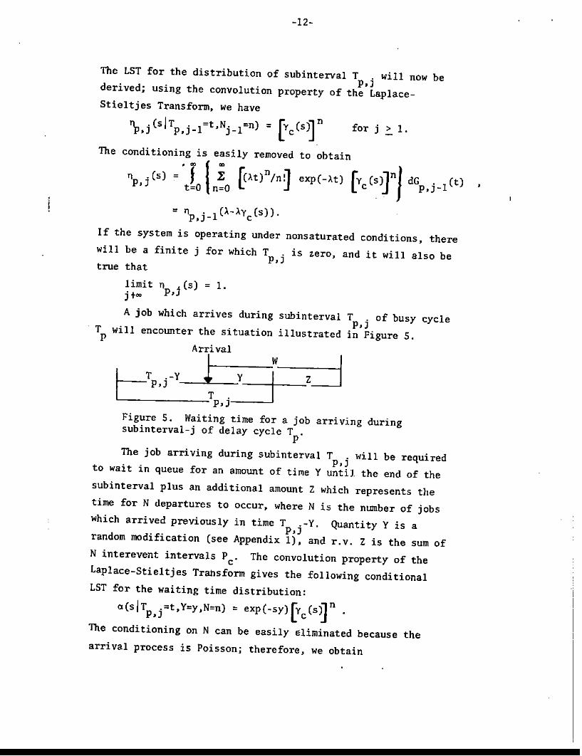
The LST for the distribution of subinterval T . will now bePol
derived; using the convolution property of the Laplace-Stieltjes Transform, we have
!L .(sIT . l=t,N. I=n) = [y (s)1 n for j > l.p,J P,J- J- C J
The
dG • I(t)P,J -
If the system is
will be a finite
true that
operating under nonsaturated conditions. there
j for which T . is zero. and it will also beP, J
limitj teo
n . (s) = l.P,]
arriving during
A job which arrives during subinterval
T will encounter the situation illustratedP
Arri val
I-__T .-Y-l--Y-__-_--iW~~~~2=JPol
L T .. _P>J-
Figure S. Waiting time for a jobsUbinterval-j of delay cycle T
p'
T . of busy cyclep, Jin Figure 5.
The job arriving during subinterval
to wait in queue for an amount of time YT . will be requiredPol
until the end of thesubinterval plus an additional amount Z which represents the
time for N departures to occur~ where N is the number of jobs
which arrived previously in time T .-Y. Quantity Y is aPol
random modification (see Appendix I), and r.v. Z is the sum of
N interevent intervals Pc. The convolution property of the
Laplace-Stieltjes Transform gives the following conditional
LST for the waiting time distribution:
'(siT .=t,Y=y,N=n) = exp(-sy)[y (s)1 n .P~J c ]
The conditioning on N can be easily eliminated because the
arrival process is Poissonj therefore. we obtain

-13-
o(slT .=t Y=y) •, P. J • 1:0=0 [F (t-Y))"/n] exp(-A (t-y))o (5 /Tp,j.t, Y.y,N=n),
• eXP (-5y )exp(-A(t-y))exp(A(t_y)'Yc
(5)).
Making use of the fact that Y is a random modification. we have
Prry
< Y < y+dy, t < T .. < t+dt' • dH . (t)dY/E(T .).l' - - - P,] - :J P,J P,]
The conditional LST for the waiting time of a job, given that the
arrival OCCurs during the jth subinterval of delay CYcle T J equals
o(5/arrival during T .). T1J O(5jT .•t'Y=Y)dyJ~1 .(t)/E(T .J,Pd t=O y=o P,] Pd Pd;
= [n . (A-AY (5))-n . (5j! Ih(T ')[AY (5)-A+5]). .Pd C Pd 1 l P.] c
= [n . 1(5)-n .(5)1/IE(T .)[Ay (5)-h5' J.p.J+ P,] J l P,] c ]
The probability tr. that a job arrives during subinterval T "J
J Pdgiven that the arrival takes place during delay CYcle T • ispequal to the steady-state probability that interval T . is
P,Jin progress (see Strauch [8J).
wj = pr[arrival during Tp,jlTp in progre5~ = E(Tp,j)/E(Tp
)'
The conditional LST for the waiting time of a job arriving duringT is therefore equal top
a(s!arrival during TpJ =tr.a(s/arrival during T .),
J P,J
= 1:j=O
1:j'O
["P,j+l (5)-np ,j (5)J I( E(Tp ) PYC(5)-A+~ J'
T ).P
= p-np ,o(5)] I (E(Tp ) [AYC
(5)-A+5] }
The first moment for the conditional waiting time is found
by making use of 1 'Hospital's Rule to evaluate -al(O/arrival during
Q.E.D.The above Theorem will now be used to obtain the conditional
LST and first moment for the distribution of waiting time for ajob which arrives during a busy period T .
cTHEOREM 2. The conditional LST for the distribution of the
waiting time Wof a job in the MIMIc system, given that the jobarrives during busy period T
cis given by

-14-
a(slarrival durit"g Tel = P-ve (S1 / (E(Tel [Ave(Sl-A+~J'
and the expected value for the conditional waiting time is
E(Wlarrival during Tel = AE(P~l/ [z [1-AE(Pel]]
+ E(P~)J [ZE(Pel] .
Q.E.D.
time Pc'
a special case of delay
interevent
Proof. Observe that busy period T ise
cycle T in which the delay T a is anp p, 2
Replacing n 0(5), E(T Ol and E(T Ol in THEOREM I by theP. P. P. 2
corresponding terms y (5), E(P J. and E(P ). we obtain thee e e
desired results.
Given the L~T and expectation associated with the waiting time
of a job conditioned upon its arrival during a busy period Te
•
sufficient information is available to determine correspondingresults for busy period T
k, where l < k < c.
THEOREM 3. The conditional LST for the distribution of waiting
time W for a job in the MIMIc system which arrives during a
busy period T1 , where 1 ~ k ~ c-l. is given by
a(s[arrival during Tk) = nl (k) + n2(k)~(slarrival during Tk
+1).
where "I (kl = E(Pkl/E(Tkl and "Z(kl = E(PklE(Tk+ll/E(Tkl
therefore. the expected value for the conditional waiting time is
E(Wlarrival during Tk) = n2 (k)E(W/arrival during Tk
+l).
Proof. ~uring busy period Tk• the system will be in one oftwo possible states:
State-I: exactly k jobs in system.
State-2: (k+l) or more jobs in system.
Let nl (k) and nZ(k) denote the steady-state probability that the
system is in State-l and State-Z, respectively, given that busy
period Tk is in progress. Using LEMMA 1, we have
E(Tkl = E(Pkl + AE(PklE(Tk+ll.
Observe that the first term on the right-hand side of the equation
represents the expected time that the system is in State-l during
interval Tk, and the second term is the expected time in State-Z.

,
-15-
•Using the method described in Appendix 2, we obtain the
representation for nICk) and n2(k) given above.
Because a job arriving when the system is in State-l can
immediately go into service (i.e. k < c) on an available
processor, the waiting time of the job is zero, and thereforethe conditional LST is
·a(5/State-l1 = 1.
The conditional LST for jobs which arrive during State-2 is
a(s]arrival during Tk+1J, and the random property of Poissonarrivals gives:
a(slarrival during Tk) = niCk) + u2 (k)a(s!arrival during Tk
+I)
and the expected value for the waiting time conditioned upon
arrival during Tk
is found to be
E(WITkl = rrZ(klE(WITK+1l. Q.E.D.
Using THEOREM 2 and THEOREM 3, the expected values for the
conditional waiting time in the MIMic system under the FCFS discipline
may be found for arrival during busy periods Tc
' Tc_1, ...• T1
in a
straightforward fashion. This completes the waiting time analysis
for the first type of busy period introduced in the previous section.
and we next examine the delay cycle Te
.
THEOREM 4. Given a MIMIc system. the conditional LST for the
distribution of waiting time for a job which arrives during delayTO (within delay cycle Te ) is given by
a(s[arrival during TO) =
={["0 (A-AyC(51] I {[yC(5~ C-I[5_A+AYC(5~I- "0(510(0,51 + cif [(-Aln/n~ "~nl(A10(n,51J IE(T01,
n=O
where 0(n,51 = {1-[-A/(S-Al] C-I-nI/5- {1- [-AyC(511 (5 -Al] c-l-nJI { [ye (51] e-l-n[5_A+AYe (51] ) .
It follows that
E(W/arrival during TOl = E(T~ll [ZE(Tol]
+ E(Pel {AE(T~ll [ZE(Tol] - ~I (e-l1 (l-~zl) ,

where
.1 = { (e-Z) (e-l)/Z -
[AE(TO~
-16-
e-Z1: f-A)n/n~ ngn) (A) [ce-Z)(e-I)/Z-(n-I) n/2]}1
n=O
/) and
.Z = ((e-I)
Proof. Recall
the system is
delay portion
in Figure 6.
e-Z1: ~_A)n/n~ ngn) (A) ~-I-n] I ~E(TO)] .
n=Othat delay cycle Te starts with delay TO and that
initially empty of jobs. A job arriving dUring the
of the delay cycle encounters the situation shown
Figure 6. Waiting time for a job arriving during delay TO'
Interval Y in the above diagram represents the time between the
arrival of the job and the end of delay TO; because the arrival
process is Poisson, interval Y has the distribution of a
random modification (cf. Appendix 1). If N jobs arrived to the
system during TO-Y' interval Z represents the amount of time
that the job will be delayed due to jobs which arrived earlier
during the delay. Interval Z equals zero if N is less than the
necessary for N-(c-l) departures to Occur, and this time is the
sum of N-(c-I) interevent times Pc. From the convolution
property of the Laplace-Stieltjes Transofrm, we have
.(sITo=t,N=n) = (exp(-sy) for 0,,- n "- e-Z,
exp(-sy) [Ye(S~ n-(e-l) for e-I < n
The conditioning.on the number of arrivals N ~an be removed by
taking int~ account the probability of any specified value of
N for the interval TO-Y.~
.(SITO=t,Y=y) = 1: ~A(t_y))n/n!] eXp(-A(t-y)).(sITO=t,Y=y,N=n) ,n=O

-17-
•c-z ~
= exp(-At) }; [(A(t-y))n/nl] exp(-(S-A)y)n"'Q ..
+ ry (S~ -(c-1)exp(_(A_AY (s))t)exp(-(S-A+AY (S))y)Lc ~ c c, c-2
~C(S~ -(C-1)exp(_At) n:o [cA(t-y)yc(S))n/n~ exp(-(S-A)y)
dy.exp( - (S-A)y)
85 shwOD below:
= i ITA(t-y))n/n~o
Because interval Y is a random modification, the. conditioningon Y and To'may be removed to give
m t
.(s/arriva1 during TO) = 1 r .(S/TO=t,Y=y)dy &IO(t) IE(TO
)'t=O y=o
We first consider some terms which pose a problem in the
evaluation of the above integral. Define Ql(t.n). whereO~n.::c-2J
For n=O, we have
Q1 (t,O) = [l-exp(-(S-A)til I(s-A).
For 1 ~ n ~ c-2. we obtain the following result by usingintegration by parts:
Q1 (t,n) = [(At)n/nJ I (S-A) - (A/(s-A))Q1 (t,n-1).
From thisc-2};
n=O
result it follows thatc-2
Q1 (t,n) = Q1 (t,O) }; (-A/(S-A)/
(c-z k=O c-Z-n }
+ n:1 [(At)n/n~ k:O (-V(S_A))k I(s-A).
Noting that several partial sums of geometric series appear in
the above expression and SUbstituting for Q1
(t.O), we obtain:
Ci/ Q1 (t,n) = Q1 (t,O) [1_(_A/(S_A))C-1] &-H/(S-A))]n=O 2 )I
+ (1/(S-A)) Cj; nAt)n/n~ [l_(_V(S_A))C-1-nYe-(-A/(S-A)~n=1
= - exp(-(S-A)t)[l _ (-A/(S_A))C-1]/s
+ c:e ~At)n/n] [1_(_A/(s_A))C-1-n] Is .n=O

-l~-
•Define another function Q2(t~n) to be ,
t
Q2(t,n) = ! ~AYc(S)(t-y))n/n~ exp(-(s-A)y)dy
Using the same procedure employed for the function Ql(t.n).
we obtainc-2
E Q2(t,n) = -exp(-(S-A)t){I-[-AYc
(S)/(S-AJ]C-IJ/{S-A+AYc
(S)Jn=O~ c-2
+ n:o [cAYc(S)t)n/ll~ (1-[ -AYc(S)/(S-A~C-l-n}/{S_A+AYc'(S)}.
Returning to the evaluation of a(slarrival during TO)' we havea(sjarrival during TO)
= r {exp(-AY) ci:.2
Q1
(t,n)y=O n=O
t+ [Yc(S~ -(c-l) eXP(-(A-AYc(S))t)! exp(-(S-A+AYc(S))y)dy
- [Yc(S~ -(C-l)exp(_At) :~: Q2(t,n) JdHO(t)/E(TO
)
Substituting the results for the sums of functions Ql(t.n) and
Q2(t,n) into the above equation, the evaluation of the integral
may be completed .. Rearranging term5 in the result gives the
desired expression for a(s Iarrival during TO).
The expected value for the conditional waiting time is
found by making use of l'Hospital's Rule to evaluate
-a'(Olarrival during TO)· Q.E.D.
Observing the result for E(Wjarrival during TO)' one sees certain
terms which are easily explained; e.g. we might anticipate that the
waiting time would consist of the expected length of the random
modification, E(T~)I [2E(TO)] , which is the time between the arrival
of the job and the end of delay TO. The remaining terms in the
expression are explained by making the following observation: The
time interval between the start of the delay and the arrival of the
job whose progress we are following has the same distribution as
the random modification. Referring to Figure 6. this is equivalent
to stating that the distribution of interval TO-V is identical to
and
-19-
that for interval Y. lJcfine random variable 'X as follows:
X = interval TO-V in Figure 6.
T(S) = LST for the distribution of X.
Because X has the distribution of a random modification. we have
the following results from Appendix 1:
E{X) = E{T~)/ [zE{T01 '
We define a variable N to be
arrivals during x] =n.Pr [N=n
N = Number of previous
A patient person can verifyc-22:
n=O
arrivals
that the
to the system during interval X.
following equations are true:c-22: [{_A)n/n~ T{n)(A).n,
n=D
andc-2~ Pr [N=n arrivals during X] =
n=O
= ~2-
If w~ interpret terms $1 and $2 in the above manner. the expected
length of the conditional waiting time becomes (cf. Figure 6)
E{Wlarrival during TO) = E{Y) + F.(2) ,
where the expected length of interval Z is
E(Z) = E{Pc ) {Pr [N ~ c-~ [E(NIN ~ C-1~ - (c-1)Pr [N ~ C-1]J-
Thus, we have a satisfying explanation for all terms in the
expression for the expected value of the conditional waiting time.
THEOREM 5. Given a MIMic system. the conditional LST for the
distribution of waiting time for a job which arrives during
interval Tf (within delay cycle Te) is equal to
a(sjarrival
where nf 0 (s) =,

-20- II
The expected length of the conditional waiting time is given by
E(W[arrivai during Tfl = E(P~l/ [2(I-AE(Pcl il
+E(T;'ol/ [2E(Tf ,ol] ,where
and
=E(PClIAE(TOl - :~: [c-Aln/n~ "cinl(Al'n
- (c-Il (1- :~:J-Aln/n~· ncinl (A~ J'
Proof. Interval Tf within delay cycle Te begins immediately
following delay TO and lasts until there are (c-l) or fewer
jobs in system. This means that the interval has length zero if
there are fewer than c arrivals during the delay. Interval Tf
can" be represented as the sum of an infinite number-of subintervals
Tf • k, where k ~ OJ as shown in Figure 7.
t=Tf,~LJf'I-t-Tf'2 '" LTf,n.-J· ../
Figure 7. Subintervals of interval Tf ·
Define a variable N as follows:
N = Number of jobs which arrive during delay TO.
Subinterval Tf •O is the time necessary for N-(c-l) departures to
occur, where N ~ c-l. At the conclusion of TfJO
there will be
(c-l) jobs in system (i.e. the jobs which arrived during the delay)
plus any jobs which arrived during Tf
O.•

-21-
Interval Tf may now be seen to be a special case of a
delay cycle T , and by replacing" 0(5), B(T 0)' and E(T2 0)P p, p, p,
in THEOREM 1 with corresponding terms nfJO(sl. E(T£.O) and
E(T~JO)' respectively, 'we innnediately find the conditional
LST the waiting time of a job' which finds i~terval Tf
in progress. However, we have yet to derive the LST and
moments associated with subinterval T£,O. The conditional LST
'for the distribution of Tr,O' given the number of arrivals N
which occur during delay TO' is given by
"f,O(S!TO=t,N=n) =
{ ~c (51for o < n < c-2
n- (c-l)for 'c-l < n.
The conditioning on the number of arrivals and length of
+ [Yc(s)] -(C-l){exp(-(A-AYc(s))t)
[(AYc (s)t)n/n3exp(-At)} JdIlO(t),
the w&iting
This result has a
c-l
delay TO may be removed to givem m
"f,O(S) = .t!o /:0 [(At)n/n ] "f,o(sITo=t,N=n) dIlO(t)
= Jo{:~: [(At)n/n~ ."p(-At)
c-2- l:
n=Oc-2= n:o [(_A)n/n~ n~n) (A)
c-2 }+{no(A-AYc(s))- n~o [(-AYc(S))"/nG "~n)(A) I [Yc(s~
The expressions for E(T£.O) and E(T~JO) are found directly
from -nf.O(O) and nfJO(O).
The last theorem in this section deal with
time for a job arriving during delay cycle T .e
number of interpretations which will be discussed in the next section;
at this point we note that this result can arise in the analysis of
certain nonpreemptive priority disciplines in which there is a job
class whose resource requests are so large that no concurrent
processing is possible when that class of job is in service.

duringI
during
-22-
THEOREM 6. Given a MIMic system. the conditional LST for the
distribution of waiting time Wof a job which arrives during
delay cycle Te is given by
a(slarrival during Te) ~ wOo(slarrival during TO)
'"f"(slarrival during Tf )
c-I+ ~ wko(s!arrival during Tk),
k=1
where "0 = E(To)/E(T.),
"f = E(Tf)/E(T.),
and, for 1 -.::.k ~ c-l,
E(Tk) ( 1-k-I
~_.)n/n~ n~n) (A) } /E(T.)"k = 2: .
n=O
The expected waiting time for a job which arrives during delay
cycle T is therefore equal to•E(Wlarrival during Te) = noE(W!arrival
+wt(Wlarrival
c-I• 2: "kE(W!arrival during Tk).
k=1
Proof. Given that a Poisson arrival occurs during interval T Jethe probability that the arriving job finds the system in a
particUlar state equals the steady-state probability of that
state within the delay cycle.
Delay cycle Te is the sum of delay TO and two intervals
Tf
and Tg
which constitute a delay busy period and which have
been previously defined. Recall that interval Tf starts
immediately after the delay and lasts until there are less than
c jobs in system. Interval T begins at the conclusion of Tf. gand terminates when the system is empty. Interval Tg is the
sum of (c-l) subintervals T 'J where 1 < j < c-l; thesegJJ - -
subintervals are illustrated in Figure 8.
f-_Tg'C_I--.-L-\:_2~ LTg'l-J
Figure 8. Subintervals within interval Tg.

-23-
•
less than j
of T . hasg.J
For 1 ~ j
Subinterval T I begins immediately after the conclusion ofg,c-Tf • and this subinterval ends when there are less, than c-I jobs,in system. For 1 < j < c-2, interval T . begins immediately
- - g,Jfollowing subinterval T . I and terminates when fewer than j
g,J+jobs remain in system. Subinterval T . has length zero if
g.Jjobs arrive during the delay; otherwise, the length
the distribution of a busy period T. (cf. LEMMA 1).].
< c-l. define:
T .' = length of subinterval-j of T shown in Figure 8,g,l g
H . (t) = cdf for Tg J j Jg,]
D . (s) = LST for the distribution of Tg,] g,i"Th. conditional LST for the distribution of Tg.i given that N
jobs arrived during delay TO is equal to
n .(S/To=t,N=n) =[D.(S) for j .:en,g.] J
1 forn<j.
Removing the conditioning on the number of arrivals and length
of delay TO gives the following result:~ j-I ~
ng,j(s) = f 2: [(At)n/n~ .xp(-At)+D.(S) 2: EAt)n/n] .xp(-At)dHO(t)t=O n=O ] n=jj-I
[(_A)n/n~ n (n) CA)= X p-nj (S~ + nj(s).n=O 0
By LEMMA 2, we have
E(T.) = E(TO
)
= E(TO
)
+ E(Tf ) + ECTg
) ,
+ E(Tf
) + C~I E(T .)j=l g,]
the system is in any given
defined and calculated using
The steady-state probabilities that
state during delay cycle T will be•the method of Appendix 2:
Wo = Pr [delay Toldelay cycle Te
in
= E(Ta)/E(T.);
progress] ,
Wf = Pr [interval Tfldelay cycle Te in progress] ,
= E(Tf)/E(T.);

•and, for 1 2 j < c-l.
uj = Pr [sutiinterval
= E(T .l/E(T).g,) e
Evaluating -Ill . (0). theg,j
is found to be
E(T .) = E(T.) 11 -g,] J
- ..... -
T .1 delay cycle T. in progress1g,] J
expected length of subinterval T .g,)
The expected waiting time
cycle T follows directly•
Substituting the above into the corresponding expression for
n., we obtain the steady-state probabilities as given in the)
statement of the theorem. By the random property of Poisson
arrivals. these probabilities will also be the probabilities
that an arrival finds the system in that particular state.
given that delay cycle Te
is in progress. We therefore have
a(slarrival during Te) = uoa(slarrival during TO)
+ ufa(slarrival during Tf )
c-l+ ~ u.a(slarrival during T.).
j=1 ) )
for a job arrlvlng during delay
from -a'(Olarrival during T). Q.E.D.•4. Applications and Extensions of the Method
In this section we consider a representative sample of
applications for the results derived in previous portions of this
paper. Furthermore. a discussion is given of ways in which these
results may be easily extended to deal with other MIMic queueing
models as well.
4.1 Comparison With the MIGII Queueing System
We begin by pointing out similarities in certain results for
the MIGII and MIMIc queueing systems which have been noted by a
number of authors. Consider a busy period T for the MIGII system
which is initiated by the arrival of a job to an empty system. and
define the following:,
,

T = min t:
-25-
o jobs in the M/G/] system at time 01 job in the M/G/l system at time 0+o jobs in the M/G/l system at time t
•
A = Poisson input rate for jobs to the M/G/] system;P = General processing time for a joh in the M/G/! system.
If we examine results for busy period T given in reference (6]pp. 149-155, it may be seen from LEMMA 1 that busy period T incthe MIMic system (with arrival rate A and interevent time P )cappears to have the same distribution as a busy period T in theM/G/l system when A is equal to A and where P has the samedistribution as P. Let us use symbol I~I to denote that twoc
random variables have the same distribution and symbol '=' todenote the equivalence of parameters. The above-mentioned situationmay then be described as given below:T ~ T when P ~ P and A ~ Ac c
If we examine the expected waiting time for a job in the MIMicsystem which arrives to find busy period T in progress, it is againcfound that the waiting time distribution is identical to that for anarrival to the MIGll system under the FCFS discipline which findsbusy period T taking place if again A : A and P ~ Pc' If we comparethe derivations of these results for the MIGll and MIMic systems,it becomes obvious that other MIGll results may be easily extendedto the MIMic system as illustrated in the example given below.EX~le. Waiting Time for the MIMic System Under the LCFS Rule.
Consider a MIMic system which employs the Last-Come-First-Served (LeFS)discipline at the queue so that, at a scheduling epoch, the most recentarrival is chosen for servicing; we assume here that once a job goesinto service it is processed to completion. Under both the LCFS andFCFS rules a job arriving to find fewer than c jobs in systemimmediately goes into service and therefore encounters a waiting timeof zero. Jobs are required to wait only when arrival occurs duringan interval T , and the distribution of busy period T is identicalccunder the FCFS and LCFS rules.
Results for the MIGII system under the LCFS rule given 1nreference [6]. pp. 155-158 allow us to state the following for the

-26-
MIMIc s~stem (using the same notation as used for the MIMic system
under the FCFS rule but with subscripts denoting the scheduling rule):,•
QLCFS (s Iarrival
ELGFSCW/arrival
ELCFS CWIarrl val
durlng Te) = [J-neCsil / (ECPe
) [S.A-AYeCsil}
durlng T ) = ECP2)/ (2[l-AQp )] E·CP )} ;
c c c c
durlng T ) = ECP3)/ (3 [l-AECP)] 2ECP )}.
c c c c
.A[ECp2)]2/ (2[l-AECP )]3ECP )1
e e e
of TIiEORcM 3 may then be used to obtain the conditionalThe results
waiting time distribution for arrival during busy period TkJ
where
1 < k < c. It also follows that for the MIMIc queueing system wehave similar results to those for the M/G/! system:
ELGFSCW) = EFGFSCW)
and
TIlis type of analysis can also be applied to analyze waiting time
distribution for the MIMIc system under other rules such as therandom rule as well.
4.2 Variations Using Delay Cycles
Many modifications of a simple MIMic queueing system seem to
include the concept of delay cycles in one way or another. The
following are examples of such modifications.
Ex Ie. Multi rocessor Facilit With 'Down' Pauses at the f.ndof Busy Periods.
Consider a mUltiprocessor service facility which can simultaneously
process up to c jobs at one time. Whenever the system is empty. all
c processors are assigned to some other obligation which takes a time
TO having a general distribution. The distribution of waiting time
in such a system is that for arrival during a delay cycle T derivede
earlier (cf. THEOREMs 4.5.6). We assume here that at the conclusion
of the interval TO the queue is examined and if empty another interval
TO is initiated. This will guarantee that every arrival to the systemfinds a delay cycle T
ein progress.

-27-
Example. Multichannel Facility With 'Warm-Upl Time.
Consider a multichannel system ip which the processor~ once idle,•needs some warm-up time or a setup time TO' of a general distribution,
•after the arrival of the first job. After this time TO' it starts
processing the jobs and conti~ues processing until the system is
empty. The analysis of this system is done essentially in the
same manner as for the delay cycle Teo The difference lies in the
small changes required to account for the first job which was already• iin the system at the beginning of the delay TO' This job is the one
responsible for initiating the delay cycle in which the warm-up time
acts as the delay interval. Figure 9 illustrates the important
random variables involved in the analysis.
systemempty
ini tial systemarrival empty
I-tT~f-_---L_-T;T-e-·-_-_-_~- T:_-1
L- L, ---'
Figure 9. Busy-Idle Cycle and Subintervals.• •The modified delay cycle T is comprised of subintervals TO (warm-up
• e •time), Tf (during which c or more jobs are in system), and T
gdefined
in a manner similar to the subintervals of delay cycle T. Idlee
period I is an exponentially distributed interarrival time with mean
l/~, and busy-idle cycle L is the sum of an idle period I and a•modified delay cycle T .e
E(l) = 1/), ;•E(L) = E(l) + feTe)
• • •E(Te) = E(To) + E(T
f)
It follows that
•+ E(T )
g
and the probabilities of an arrival•modified delay cycle T J given thate
finding an idle period I or
busy-idle cycle L is in progress, are'.Of
'1 = Pr[idle period I in progress] ,
= E(l)/f(L);•, = Pr[delay cycle T in progress],e e
•= E(T )/E(L).
e

-28-
Since every job arrives during a bus~-idle cycle L. the above are, .also the unconditional steady-state probabilities. Assume that
the FCFS discipline is employed; a job arriving during idle period I, .has waiting time equal to the warm-up time TO' and the unconditionalexpected waiting time is
c-2-(C-2)[I- ~
n=O
•T ).
e
job arriving during
essentially the same
~eE(Wlarrival during
•E(T )g
The ~onditional expected waiting time of a•modified delay cycle T can be ohtained ine
manner as for delay cycle T. Refer to the derivation and discussione • •
for'LEMMA 2; if N jobs arrive during delay TO' the remainder of Te
is the sum of busy periods TN+1J TN•... JT] (rather than TN through
TI as for delay cycle T). The presence of the initial job at the• estart of interval T requires the changes shown below for the
e ••expected len~th of subintervals T
fand T
g:
E(T;) = E(Tc ) {pr[N::c-I] E(NIN>C-I)-(c-2)pr[N::c_Ij}
c-2= E(Tc ) {FE(T~)- n:o [c-A)n/n~ nan) (A)i
nan) (A)]},c-I
, ~ E(Tk)Pr[N::k-lj ,k,1
c-I k-2
, E(TI ) + k:2 E(Tk) {I - n:o [(-A)n/n!Jnan) (A) } .
•The expected conditional wa1tlng time for an arrival during TO
requires similar changes as compared to the results given in THF.OREM 4:
. - (c-2) [I -
where T(S) = •, LST for TO
•The expected conditional waiting times for arrival during Tf
have the
same representation as given in TlffiOREM 5 except that we must include•changes to the distri~ution of subinterval-O of Tfo That is, we view

•nf, 0 (s)
-I.J-
• •random variable Tf as being composed of subintervals Tf
. (cf.oJ •Figure 7) for j > O. If N jobs arrive during the warm-up time TO
•(~n addition to the first arrival which initiated TO)' subinterval
Tf 0 is the time needed for (N+l)-(c-l) departures to occur. assuming, .that N is greater than or equal ~o (c-l). If we denote the number
•of arrivals during sUbinterval-j of Tf
by N. ( j > 0). subintervRl• J -
Tf . is the time needed for N. 1 departures to occur. Comparing,J J-
these definitions with those given for the subintervals of Tf
of
THEOREM S. we see that only the definition for subinterval-a has•been changed. The waiting time analysis for T
fapplies also to T
f•if we substitute results for subinterval-a of Tf
. Denote the LST• • •for the distribution of Tf a (i.e. subinterval-a of T
f) by n
f0 (S)j, ,
the conditional LST given that N arrivals occur during the warm-up•
time TO is given as
• •nf,o(sITo=t.N=n) =( 1 if 0 < n < c-2.
[Yc(S)]n-(c-2)if n > c-2
Removing the conditioning we obtainc-3
= 1: [(-A)n/nl]n~n)(A)n=O
c-3 J+ (no(A-AYc(S)) - n:o [(-AYc(S))n/n!]n~n)(A) /[Y
C(5)]C-2 .
•The first two moments of Tf,O
E(T;,O) = E(Pc ) (AE(T~)
• 2E((Tf,O) )
are directly found to be
c-31: [(-A)n/n!]n~n)(A).n
n=Oc_3
- (c-2) p. - /:0 [(-A)n/n!]n~n)(A1}
c-3= [E(Pc)]2 (-2(C-2) [AE(T~) - n:o [(-A)n/nl]n~n)(A).n]
c-3 (n)n1: [(-A) /n!]n
o(A)n.(n-1)
n=Oc-3 ()}
+ (c-2)(c-1) [1 n:o [(-A)n/nl]non (A)]
c-31: [(_A)n/n!]n~n)(A).n
n=Oc-3
- (c-2) F- 1: [(-i)n/nlj',Jn)r')'J.n=O :J

-30-
..•and THEOREM 5 gives E(W]arrival during Tfl by replacing E(T
f0) and
2 .. * 2 J
E(Tf oj with E(Tf oj and E((Tf oj J, respectively.• , * J
Random variable T may be viewed as being a sequence of subinter-.,. * g * '
vals T l' T 2'·'. J T 1 (defined as the subintervals of T giveng,c- g,c- g • .,. g*in llffiOREM 6). Given that T k has length greater than zero, T kg, g.
: has the distribution of busy period TkO In order to apply THEORFM 6,
we need only modify the probability ~kJ for 1 ~ k ~ c-l. that an•
arrival during T finds subinterval r* .in progress; the expected.,. e g.klength of T k is given byg,
•E(Tg,kJ = E(TkJ*Pr[N ~ k-l],
•where N is the number of arrivals during TO'
It follows from THEOREM 6 that•E(W!arrival during Te) = wOE (WI arrival during
+rrrE(Wlarrival duringc-l
+ ~ wkE(Wlarrivalk=l
This completes the waiting time analysis for the example prohlem.
4.3 Variations Using Busy Periods
We next consider an example in which results for the husy period
Tk of LEMMA 1 find application. This will allow an analysis of the
waiting time results of THEOREMS 2 and 3.
Example. Multiprocessor Facility With Start-Up Based on
Number in System.
Consider a multichannel system in which due to the high cost of
starting and servicing, the processor waits until its use is
warranted by a certain number. M. of jobs which have arrived to
the system. Once the processor starts processing, it continues
in operation until the system is empty. Let us assume that M < c
in the analysis which follows; Figure 10 illustrates various
random variables of interest for the given example problem.

-31-
Figure 10. Busy-idle Cycle and Subintervals.
system first secondempty arri val arrival
. 10---1-11_-,:+ ...L'- L
Mtharrival.t Til L
T
TM_1-l
A busy period T in this case consists of the sum of busy periods
TM' TM_1J." • T1 (here it is appropriate tQ interpret Tk
as the
time needed to achieve an overall reduction, by one, of the jobs
in system). We identify Midle periods, defined as given belowfor 0 2. j < M-I:
T. = idle period during which j jobs are in system; thisJ interval represents an interarrival time for a Poisson
process with rate A and therefore E(I.) = l/A.J
Busy-idle cycle L is the sum. of busy period T and the M idle periods.
from which it follows thatM-I M
F.(L) = E E(l.) + E E(Tk) • where F.(Tk
) is given by LEMMA I.j=D J k=1
A job arriving during idle period T. becomes the (j+l)-st job inJ
system and so must wait until (M-(j+l) additional jobs arrive
before going into service. It follows that for 0 ~ j ~ M-l,
E(Wlarrival during I.) = (I/A) (M-j-I).J
during I.)J
[E(I.)/E(L)]*E(WlarrivalJ
The unconditional waiting time is easily obtained by utilizing the
method of Appendix-2 to find the steady-state probability that anarrival finds the system in any particular state.
M-IE(W) = E
j=DM
• E [E(Tk)/E(L)]*E(Wlarrival during Tk
)k=1
where E(Wjarrival during Tk) is found using THEOREMs 2 and 3.
4.4 Unequal Channel-Service.Rates
In some practical situations it is possible to have unequal
channel-service-rates in multichannel systems. For example, a
job with highest internal priority in a multiprogrammed computer
system receives preferential treatment and may in effect get a

,• •
-32-
higher service rate.
Let the service-rate for channel-j be
and let the channels be ordered such that
1-1 where 1 < J" _< C,j ,
> ••• > lJ" •C
Assume that it is possible to have instantaneous switching of~channels
and that, when there are j jobs in service, the first j channels
will be servicing jobs. A new job, when started. receives the
highest available service rate. The service rate lJi
of a job.
being processed, is instantaneously changed to the higher rate
lJ i _1 as socn as this rate is available. Any rate lJi is said to be
available when the job with that rate is either finished or when
that job's service rate is changed to a higher rate. For example,
consider a 3-channel system with all three servers busy. Suppose
that the job with rate 1-1} is finished; the job with rate ~2 will
then have rate ~l' and the job with rate ~3will then have rate ~2.
If the queue is not empty, the first job in the queue will have
its processing started and will receive service at rate ~3.
The analysis of busy period Tk of LEMMA 1 and correspond~ng
conditional waiting time results given in THEOREMS 2 and 3 may be
easily modified to deal with this case. In LEMMA 1, THEOREM 2,
and THEOREM 3, it is only necessary to change the distrihution of
'j
random variable Pk (the aggregate of k Poisson
with the jobs in service) as shown below for I
processes•
< k < c:
associated
If it is not possible to have switching of service rates, the
analysis quickly becomes cumbersome for increasing values of c,
although small values such as c =2 can be readily handled.

s. Summary.
This paper has demonstrated that the method of busy period
analysis previously used for treating the MIGII queueing system
can be extended to deal with the MIMIc queueing system as well.
Closed-form results have been presented for the distribution of two major
types of busy periods arising in the MIMIc system and for the
distribution of waiting time (under the FCFS discipline) for
an arriving job which finds a particular type of busy period inprogress.
A number of examples have been presented which show that
these results may be usefully applied and extended to deal with
a number of different models for mUltiprocessor systems. Theseexamples included the following:
MIMIc System Under the LCFS RUle.
Multiprocessor Facility With I Down I Pauses at the End ofBusy Periods.
Multichannel Facility With 'Warm-Up I Time.
Multiprocessor Facility With Start-Up B~sed on Numberof Jobs in System.
Multichannel System. With Unequal Channel-Service-Rates.
It is the hope of the authors that the results in this paper
will serve not only to illustrate the usefUlness of the method
of busy period analysis for MIMIc systems but also to give the
reader insigh~ in the characteristics of this class of
multiprocessor queueing systems.
,
-34-
•References
1. Omahen, K. J. Analytic mode~s of multiple resource systems.Ph.D. Thesis, Committee on Information Sciences, Universityof Chicago, June, 1973.
2. Marathe, V. P. Priority queueing systems with simultaneousserver requirements. Ph.D. Thesis, Operations Research,Cornell University. May, 1972.
3. Omahen, K. and Marathe. V. A queueing model for a multiprocessor system with partitioned memory. Technical ReportCSD-TR 132, Dept. of Computer Science, Purdue University.January, 1975.
4. Cobham, A. Priority assignment in waiting line problems.,Op'Ee...ra"t"i~o"n"s,--"R"e=-s e"a",r~c"h,--=-2 • 1 (1954).
5. Avi-Itzhak. B., Maxwell, W. L., and Miller, L. W.with alternating priorities. Operations Research
Queueing13 (1965), 306-318.
6. Conway, R. W., Maxwell. W. L., and Miller. L. W. Theory ofSchedUling. Addison-Wesley, Reading, Massachusetts. 1967.
7. Cox, D. R. Renewel Theory. London: Methuen, 1962.
8. Strauch, R. E. When a queuecustomer as to an observer.140-141.
looks the same to an arrivingManagement Science 17 (1970),
9. Widder, D. V. The Laplace Transform. Princeton UniversityPress, Princeton, New Jersey, 1946.
10. Little, J. D. C. A proof of the queueing formUla L = AW.Qperations Research 9 (1961), 383-387.

-35-
,
;
APPENDIX"I
PROPERTIES OF POISSON PROCESSES,Consider a Poisson process with rate A; such a process is
characterized by a'sequence of interevent times which are independentand exponentially distributed. Define:
T = time between successive events for the Poisson process.
G(t) = Pr[T ~ t] = 1 - exp(-At), t ~ O.
yes) = LST for the distribution of T = A/CS+A).
The first and second moments for the distribution of interevent times areE(T) = IIA, and E(T2) = 2/A 2.
Define another random variable as follows:
N(t) = NUmber of events which take place during interval tfor a Poisson process with rate A.
The distributlon for NCt) has the following characteristics:
Pr[N(t) = nJ = [(At)n/n !] exp(-At) for integer n ~ 0,E(N(t)) = At for t > O. •
i=i
nX A..
1
The Poisson process has many properties which are utilized in
the body of this paper; these properties are summarized below. The
proofs for these properties are available in a number of textbooks(e.g. see Reference [6]).
AI.l The Memoryless Property
Suppose that we are interested in the distribution for inter
event time T, given that a certain amount of time y has already
passed without an event taking place. Poisson processes have theunique property that
Pr[T < y+tlT > y] = 1 - exp(-At).
The process is memoryless in the sense that the distribution for
the remaining time until the next event does not depend upon the
amount of time which has passed without an event taking place.
AI.2 Aggregation and Branching of Poisson Processes
AI.2.1 Assume that there are n Poisson processes simultaneously in
progress and that events associated with the ~th process are taking
place at rate Ak , where k = 1,2, ... ,n. The aggregate of these processes
will be defined such that events associated with each of the n Poisson
processes will be considered to be events for the aggregate.9 The
aggregate of these Poisson processes is also Poisson with rate A =

.\-36-
Al.2.2 Consider the situation in which events.~ssociated with a
Poisson process with rate A are su~jected to a decision process
whereby each event is (instantly) mapped into one uf'n classes.
Every time an event occurs, the decision process maps the event
~nto class-k independently and with probability Ak
, where K = 1.2, ...•n
and where the sum of ,these probabilities is equal to one. If we
define n processes, where the kth process consists of those events
mapped into class-k, each process constitutes a Poisson process
with rate Alc" Therefore, we have the situation in which a Poisson
process branches into independent Poisson processes.
Al.2.3 As a consequence of AI.2.1 and Al.2.2, we obtain the following
result. Given that we have an aggregate of n Poisson processes and
an event occurs, the probability that the'event is associated with the
kth Poisson process (1 ~ k ~ n) is equal to Ak/A.
Al.3 The Random Property
Poisson events are frequently referred to as "random events"
because of the property described below. Given that an event occurs
during an interval of length t, the instant at which the event takes
place is uniformly distributed over the length of the interval, i.e.
Pr[y ~ instant of event occurrence ~ y+dylevent in t]
= dy/t for 0 ~ y ~ t.
AI.4 The Random Modification
Assume that an event associated with a
the end of interval X; this interval Y will
place during interval X.of the Poisson event and
Consider the time
Poisson process takes
Y between the occurrence
be called the random modification. Define:
X = length of some interval haVing an arbitrary distribution,
G(x) = cdf for r.v. X,
yes) = LST for the distribution of X;
Y = length of random modification of variable X.H(y) = cdf for r.v. Y,
T(S) = LST for the distribution of Y.
We have the following results for the random modification:
(a) Pr[y ~ y 2 y+dy, x ~X ~ x+dx] = dG(x)dy/E(X), o~<x. O~x<~.
(b) dH(y) = [l-G(y)]dy/E(X) for 0 < y < 00.
- k - k+l(e) T(5) = [1-Y(5)]/[5E(X)], and E(Y ) = E(X )/{(k+1)E(X)),k ~ 1.

within interval T,
-37-
APPENDIX-2
A METHOD POR DETERMINING STEADY-STATE PROBABILITIES
We will often be interested in determining the steady-state
probability that the system is in some specified state, given1that
an interval T is in progress. The possible states of the system
during interval T will be denoted by 51,52, ... , So" Associated
with each state Skis a random variable Xk which represents the
amount of time that the system remains in state Sk upon a transition
to that state. where k = 1.2•... ,n. For 1 2 k ~ n. define:
Nk =(1 if Xk is in progress
o otherwise.
The steady-state probability that the system is in state Sk given
that interval T is in progress is therefore
Pr[SklTj = E(Nk) for k = 1,2, ... ,n.
If we examine the system operation only during those times that
intervals of type T are in progress. the intervals of type T appear
to be initiated at rate A given by
" = 1/E(T),
and intervals of type Xk appear to be initiated at rate Ak
given as
"k = r k",
where r k is the relative rate at which intervals Xx are initiated
given that an interval T is in progress.
Using Little's Equation [10] ,we find
E(Nk) = "kE(Xk),
= rkE(~)/E(T);
therefore, we have the following result:
Pr[Sk!Tj = rkE(Xk)/E(T).
If there are n mutually exclusive and exhaustive system states during T,
it will obviously be the case that
nX rkE(~)/E(T) = !
k=1or
nE(T) • X rkE(Xk)
k=!