Embed Size (px)
Citation preview
Analysis and Application of Optimization
Techniques to Power System Security and
Electricity Markets
by
Jose Rafael Avalos Munoz
A thesis
presented to the University of Waterloo
in fulfillment of the
thesis requirement for the degree of
Doctor of Philosophy
in
Electrical and Computer Engineering
Waterloo, Ontario, Canada, 2008
c© Jose Rafael Avalos Munoz 2008

I hereby declare that I am the sole author of this thesis. This is a true copy of the
thesis, including any required final revisions, as accepted by my examiners.
I understand that my thesis may be made electronically available to the public.
ii
Abstract
Determining the maximum power system loadability, as well as preventing the sys-
tem from being operated close to the stability limits is very important in power
systems planning and operation. The application of optimization techniques to
power systems security and electricity markets is a rather relevant research area in
power engineering. The study of optimization models to determine critical operat-
ing conditions of a power system to obtain secure power dispatches in an electricity
market has gained particular attention. This thesis studies and develops optimiza-
tion models and techniques to detect or avoid voltage instability points in a power
system in the context of a competitive electricity market.
A thorough analysis of an optimization model to determine the maximum power
loadability points is first presented, demonstrating that a solution of this model
corresponds to either Saddle-node Bifurcation (SNB) or Limit-induced Bifurcation
(LIB) points of a power flow model. The analysis consists of showing that the
transversality conditions that characterize these bifurcations can be derived from
the optimality conditions at the solution of the optimization model. The study
also includes a numerical comparison between the optimization and a continuation
power flow method to show that these techniques converge to the same maximum
loading point. It is shown that the optimization method is a very versatile technique
to determine the maximum loading point, since it can be readily implemented
and solved. Furthermore, this model is very flexible, as it can be reformulated to
optimize different system parameters so that the loading margin is maximized.
The Optimal Power Flow (OPF) problem with voltage stability (VS) constraints
is a highly nonlinear optimization problem which demands robust and efficient so-
lution techniques. Furthermore, the proper formulation of the VS constraints plays
a significant role not only from the practical point of view, but also from the mar-
ket/system perspective. Thus, a novel and practical OPF-based auction model is
proposed that includes a VS constraint based on the singular value decomposition
(SVD) of the power flow Jacobian. The newly developed model is tested using
iii

realistic systems of up to 1211 buses to demonstrate its practical application. The
results show that the proposed model better represents power system security in
the OPF and yields better market signals. Furthermore, the corresponding so-
lution technique outperforms previous approaches for the same problem. Other
solution techniques for this OPF problem are also investigated. One makes use of
a cutting planes (CP) technique to handle the VS constraint using a primal-dual
Interior-point Method (IPM) scheme. Another tries to reformulate the OPF and
VS constraint as a semidefinite programming (SDP) problem, since SDP has proven
to work well for certain power system optimization problems; however, it is demon-
strated that this technique cannot be used to solve this particular optimization
problem.
iv

Acknowledgments
I would like to express my sincere gratitude to Prof. Claudio A. Canizares for his
guidance, patience, and support throughout my Ph.D studies. His contribution to
my life is simply priceless, thank you for everything Professor. I also offer an special
acknowledgment to Prof. Miguel F. Anjos for all his suggestions and motivation.
Their professionalism and dedication is a source of inspiration. It was a great honor
to work with them.
An important recognition to my examining committee members: Prof. Kankar
Bhattacharya, and Prof. Anthony Vannelli from the Electrical and Computer Engi-
neering Department, and specially to Prof. Paul Calamai from the Systems Design
Engineering Department for his important comments.
Special thanks to my officemates for their friendship and unique environment
in the EMSOL lab: Hemant Barot, Amirhossein Hajimiragha, Hassan Ghasemi,
Hamid Zareipour, Sameh Kodsi, Ismael El-Samahy, Hosein Haghighat, Mohammad
Chehreghani, and Chaomin Luo. It was such a nice pleasure to learn many things
from their cultures and values; they added another spice to my life. The continuous
motivation from my friends in Mexico and Waterloo who always cheered me up and
made me smile is also appreciated. I also offer a sincere acknowledgment to Fr. Bob
Liddy for all his blessings.
A bouquet of roses to Prof. Sukesh Ghosh and lovely Mrs. Nandita Ghosh for
their kindness and support, and for teaching me important lessons about life. I
discovered a treasure in your words and heart. Mysterious events happen in life,
and I do believe that our encounter is one of them.
I wish I could put all the stars in the Universe in a vault to express with each
one of them my love for my wonderful parents and family. Thank you for the best
gift of my life and for making my dream come true. Nothing would have been
possible without your support and love.
I am grateful for the scholarship granted by CONACyT Mexico.
v

Dedication
This thesis is dedicated to all my family, and to the other part of my life who
is yet to come...
vi
Contents
1 Introduction 1
1.1 Research Motivation . . . . . . . . . . . . . . . . . . . . . . . . . . 1
1.2 Literature Review . . . . . . . . . . . . . . . . . . . . . . . . . . . . 2
1.2.1 Voltage Stability . . . . . . . . . . . . . . . . . . . . . . . . 3
1.2.2 OPF-based Auction Models . . . . . . . . . . . . . . . . . . 5
1.3 Objectives . . . . . . . . . . . . . . . . . . . . . . . . . . . . . . . . 7
1.4 Thesis Outline . . . . . . . . . . . . . . . . . . . . . . . . . . . . . . 8
2 Background Review 10
2.1 Introduction . . . . . . . . . . . . . . . . . . . . . . . . . . . . . . . 10
2.2 Voltage Stability Analysis . . . . . . . . . . . . . . . . . . . . . . . 10
2.2.1 Effects of Increasing Demand . . . . . . . . . . . . . . . . . 11
2.2.2 System Models . . . . . . . . . . . . . . . . . . . . . . . . . 13
2.2.3 Bifurcation Analysis . . . . . . . . . . . . . . . . . . . . . . 14
2.3 Power System Security . . . . . . . . . . . . . . . . . . . . . . . . . 20
2.3.1 Security Assessment . . . . . . . . . . . . . . . . . . . . . . 21
2.3.2 Available Transfer Capability . . . . . . . . . . . . . . . . . 22
vii
2.3.3 Loading Margin . . . . . . . . . . . . . . . . . . . . . . . . . 23
2.4 Voltage Stability Analysis Tools . . . . . . . . . . . . . . . . . . . . 25
2.4.1 Continuation Power Flow (CPF) . . . . . . . . . . . . . . . 25
2.4.2 OPF-based Direct Method (OPF-DM) . . . . . . . . . . . . 26
2.5 Optimal Power Flow Models with Security Constraints . . . . . . . 30
2.5.1 Security-Constrained OPF (SC-OPF) . . . . . . . . . . . . . 31
2.5.2 Voltage-Stability-Constrained OPF (VSC-OPF) . . . . . . . 32
2.5.3 Locational Marginal Prices (LMP) . . . . . . . . . . . . . . 36
2.6 Optimization Methods . . . . . . . . . . . . . . . . . . . . . . . . . 38
2.6.1 Primal-Dual Interior-Point Method (IPM) . . . . . . . . . . 38
2.6.2 Semidefinite Programming (SDP) . . . . . . . . . . . . . . . 44
2.7 Summary . . . . . . . . . . . . . . . . . . . . . . . . . . . . . . . . 45
3 Analysis of the OPF-DM 46
3.1 Introduction . . . . . . . . . . . . . . . . . . . . . . . . . . . . . . . 46
3.2 Theoretical Analysis of the OPF-DM . . . . . . . . . . . . . . . . . 47
3.3 Numerical Examples . . . . . . . . . . . . . . . . . . . . . . . . . . 68
3.3.1 Practical Implementation Issues . . . . . . . . . . . . . . . . 68
3.3.2 Numerical Results . . . . . . . . . . . . . . . . . . . . . . . 69
3.4 Summary . . . . . . . . . . . . . . . . . . . . . . . . . . . . . . . . 76
4 Practical Solution of VSC-OPF 77
4.1 Introduction . . . . . . . . . . . . . . . . . . . . . . . . . . . . . . . 77
4.2 Proposed Solution Method . . . . . . . . . . . . . . . . . . . . . . . 78
4.2.1 Singular Value Decomposition (SVD) . . . . . . . . . . . . . 78
viii
4.2.2 MSV VSI of Invariant Jacobian . . . . . . . . . . . . . . . . 80
4.2.3 Updating Algorithm . . . . . . . . . . . . . . . . . . . . . . 85
4.3 Numerical Results . . . . . . . . . . . . . . . . . . . . . . . . . . . . 86
4.3.1 Effect of Proposed VS Constraint . . . . . . . . . . . . . . . 86
4.3.2 Efficiency of the Proposed Method . . . . . . . . . . . . . . 88
4.3.3 Comparison of VSC-OPF Formulations . . . . . . . . . . . . 88
4.3.4 Proposed VSC-OPF vs SC-OPF . . . . . . . . . . . . . . . . 95
4.3.5 Generation Cost Minimization in a Real System . . . . . . . 107
4.4 Summary . . . . . . . . . . . . . . . . . . . . . . . . . . . . . . . . 110
5 Other Approaches to Solving the VSC-OPF 111
5.1 Introduction . . . . . . . . . . . . . . . . . . . . . . . . . . . . . . . 111
5.2 Solving the VSC-OPF via CP/IPM . . . . . . . . . . . . . . . . . . 111
5.2.1 Proposed Technique . . . . . . . . . . . . . . . . . . . . . . 112
5.2.2 Numerical Results . . . . . . . . . . . . . . . . . . . . . . . 130
5.3 Solving the VSC-OPF via SDP . . . . . . . . . . . . . . . . . . . . 137
5.4 Summary . . . . . . . . . . . . . . . . . . . . . . . . . . . . . . . . 140
6 Conclusions 141
6.1 Summary . . . . . . . . . . . . . . . . . . . . . . . . . . . . . . . . 141
6.2 Contributions . . . . . . . . . . . . . . . . . . . . . . . . . . . . . . 144
6.3 Future Work . . . . . . . . . . . . . . . . . . . . . . . . . . . . . . . 145
A Test Systems 146
A.1 6-bus Test System . . . . . . . . . . . . . . . . . . . . . . . . . . . . 146
ix

A.2 CIGRE-32 Test System . . . . . . . . . . . . . . . . . . . . . . . . . 148
A.3 1211-bus Test System . . . . . . . . . . . . . . . . . . . . . . . . . . 154
Bibliography 155
x
List of Figures
2.1 QS(V ) and QL(V ) characteristics and equilibrium points . . . . . . 12
2.2 SNB without QG limits. . . . . . . . . . . . . . . . . . . . . . . . . 16
2.3 Stable limit point (LIDB) followed by a SNB. . . . . . . . . . . . . 16
2.4 Unstable limit point (LISB). . . . . . . . . . . . . . . . . . . . . . . 17
2.5 LISB preceded by a LIDB. . . . . . . . . . . . . . . . . . . . . . . . 17
2.6 ATC evaluation with dominant voltage limits. . . . . . . . . . . . . 23
2.7 Predictor-corrector scheme in the CPF. . . . . . . . . . . . . . . . . 25
2.8 σc versus λc changes for different power dispatches. . . . . . . . . . 35
2.9 Primal-dual IPM . . . . . . . . . . . . . . . . . . . . . . . . . . . . 41
3.1 Solution points for the system (3.1). . . . . . . . . . . . . . . . . . . 48
3.2 Solution points for the system (3.4). . . . . . . . . . . . . . . . . . . 49
3.3 Generator-Infinite Bus system . . . . . . . . . . . . . . . . . . . . . 50
3.4 Generator-Infinite Bus system . . . . . . . . . . . . . . . . . . . . . 52
3.5 Generators’ PV curve for the 6-bus system: The base case exhibits
a LISB. . . . . . . . . . . . . . . . . . . . . . . . . . . . . . . . . . 69
3.6 Generators’ PV curve for the 6-bus system: A contingency scenario
shows a LIDB followed by an SNB. . . . . . . . . . . . . . . . . . . 70
xi

3.7 Generators’ PV curve for the 6-bus system: SNB with no QG-limits. 70
3.8 PV curve for the CIGRE-32 test system: The base case exhibits an
SNB. . . . . . . . . . . . . . . . . . . . . . . . . . . . . . . . . . . . 73
3.9 PV curve for the CIGRE-32 system: SNB with no QG-limits. . . . . 73
4.1 PV curves, and MSV of J and JPF for a 6-bus test system: (a) SNB
neglecting QG-limits; (b) LIB considering QG-limits. . . . . . . . . . 81
4.2 PV curve, and two critical MSV for J and JPF at the the same
loading point; ∆λ defines a security margin. . . . . . . . . . . . . . 83
4.3 MSV of JPF for the CIGRE-32 test system considering QG-limits. . 84
4.4 MSV at every iteration when σc is increased from 0 to 4.98, and
when increased from 4.262 to 4.98. . . . . . . . . . . . . . . . . . . 89
4.5 MSV at the optimum with respect to the loading factor (a) for (4.4),
and (b) for (2.24). . . . . . . . . . . . . . . . . . . . . . . . . . . . . 91
4.6 ESCO 3 power with respect to the loading factor for the 6-bus system. 92
4.7 GENCO 3 power with respect to the loading factor for the 6-bus
system. . . . . . . . . . . . . . . . . . . . . . . . . . . . . . . . . . . 92
4.8 LMP 6 with respect to the loading factor for the 6-bus system. . . . 93
4.9 Objective function with respect to the loading factor for the 6-bus
system. . . . . . . . . . . . . . . . . . . . . . . . . . . . . . . . . . . 93
4.10 ESCO 3 voltage with respect to the loading factor for the 6-bus system. 94
4.11 GENCO 3 reactive power with respect to the loading factor for the
6-bus system. . . . . . . . . . . . . . . . . . . . . . . . . . . . . . . 94
4.12 ESCO 1 power with respect to the loading factor for the 6-bus system. 98
4.13 ESCO 2 power with respect to the loading factor for the 6-bus system. 98
4.14 ESCO 3 power with respect to the loading factor for the 6-bus system. 99
xii

4.15 GENCO 1 power with respect to the loading factor for the 6-bus
system. . . . . . . . . . . . . . . . . . . . . . . . . . . . . . . . . . . 99
4.16 GENCO 2 power with respect to the loading factor for the 6-bus
system. . . . . . . . . . . . . . . . . . . . . . . . . . . . . . . . . . . 100
4.17 GENCO 3 power with respect to the loading factor for the 6-bus
system. . . . . . . . . . . . . . . . . . . . . . . . . . . . . . . . . . . 100
4.18 Objective function with respect to the loading factor for the 6-bus
system. . . . . . . . . . . . . . . . . . . . . . . . . . . . . . . . . . . 101
4.19 Locational Marginal Price (LMP) at bus 1 with respect to the loading
factor for the 6-bus system. . . . . . . . . . . . . . . . . . . . . . . 101
4.20 Locational Marginal Price (LMP) at bus 2 with respect to the loading
factor for the 6-bus system. . . . . . . . . . . . . . . . . . . . . . . 102
4.21 Locational Marginal Price (LMP) at bus 3 with respect to the loading
factor for the 6-bus system. . . . . . . . . . . . . . . . . . . . . . . 102
4.22 Locational Marginal Price (LMP) at bus 4 with respect to the loading
factor for the 6-bus system. . . . . . . . . . . . . . . . . . . . . . . 103
4.23 Locational Marginal Price (LMP) at bus 5 with respect to the loading
factor for the 6-bus system. . . . . . . . . . . . . . . . . . . . . . . 103
4.24 Locational Marginal Price (LMP) at bus 6 with respect to the loading
factor for the 6-bus system. . . . . . . . . . . . . . . . . . . . . . . 104
4.25 ESCO 2 voltage level with respect to the loading factor for the 6-bus
system. . . . . . . . . . . . . . . . . . . . . . . . . . . . . . . . . . . 104
4.26 GENCO 2 reactive power with respect to the loading factor for the
6-bus system. . . . . . . . . . . . . . . . . . . . . . . . . . . . . . . 105
4.27 MSV at the optimum of the VSC-OPF and SC-OPF. . . . . . . . . 105
4.28 ATC with respect to system loading for the 6-bus system. . . . . . . 106
xiii

4.29 TTC with respect to system loading for the 6-bus system. . . . . . 106
4.30 Generation re-dispatch when the VSC-OPF is applied to a 1211-bus
test system. . . . . . . . . . . . . . . . . . . . . . . . . . . . . . . . 108
4.31 Increment in bus voltages when the VSC-OPF is applied to a 1211-
bus test system. . . . . . . . . . . . . . . . . . . . . . . . . . . . . . 108
5.1 Graphic representation of the proposed CP/IPM algorithm. . . . . 112
5.2 CP/IPM flow chart to solve the VSC-OPF . . . . . . . . . . . . . . 115
5.3 MSV of the power flow Jacobian using a Newton method: (a) flat
start; (b) power flow start. . . . . . . . . . . . . . . . . . . . . . . . 119
5.7 Objective function using a Newton method: (a) flat start; (b) power
flow start. . . . . . . . . . . . . . . . . . . . . . . . . . . . . . . . . 123
5.8 Objective function using a predictor-corrector method: (a) flat start;
(b) power flow start. . . . . . . . . . . . . . . . . . . . . . . . . . . 124
5.9 Number of iterations using a Newton method: (a) flat start; (b)
power flow start. . . . . . . . . . . . . . . . . . . . . . . . . . . . . 125
5.10 Number of iterations using a predictor-corrector method: (a) flat
start; (b) power flow start. . . . . . . . . . . . . . . . . . . . . . . . 126
5.11 Cuts at every iteration using a Newton method: (a) flat start; (b)
power flow start. . . . . . . . . . . . . . . . . . . . . . . . . . . . . 127
5.12 Cuts at every iteration using a Predictor-corrector method: (a) flat
start; (b) power flow start. . . . . . . . . . . . . . . . . . . . . . . . 128
5.13 Final value of σ(k) when the cut is added using different criteria:
(a) ξ = NPF (b) ξ = 1 × 10⁻³. In each case, the top two figures
correspond to the Newton method; the two in the bottom correspond
to the predictor-corrector method; the two on the left correspond to
flat start, and power flow start is on the right. . . . . . . . . . . . . 129
xiv

5.14 MSV of the power flow Jacobian using a predictor-corrector method
with a power flow start for the CIGRE-32 test system. . . . . . . . 130
5.15 MSV at every iteration in the CP/IPM when solving the CIGRE-32
system. . . . . . . . . . . . . . . . . . . . . . . . . . . . . . . . . . . 132
5.16 Feasibility of (a) the objective function and (b) the power flow equa-
tions (equality constraints) in the CP/IPM when solving the CIGRE-
32 system. . . . . . . . . . . . . . . . . . . . . . . . . . . . . . . . . 133
5.17 The box encloses the iterations at which some cuts are added in the
CP/IPM when solving CIGRE-32 system. . . . . . . . . . . . . . . 134
5.18 Feasibility parameters in the CP/IPM when solving the CIGRE-32
system. . . . . . . . . . . . . . . . . . . . . . . . . . . . . . . . . . . 137
5.19 2-bus system . . . . . . . . . . . . . . . . . . . . . . . . . . . . . . . 138
A.1 6-bus test system. . . . . . . . . . . . . . . . . . . . . . . . . . . . . 147
A.2 CIGRE-32 test system. . . . . . . . . . . . . . . . . . . . . . . . . . 149
xv
List of Tables
3.1 OPF-DM vs CPF for the 6-bus test system . . . . . . . . . . . . . . 71
3.2 Comparison of the OPF-DM vs CPF for the CIGRE-32 system . . . 74
4.1 Structure and dimensions of J . . . . . . . . . . . . . . . . . . . . . 82
4.2 Progress of the unitary vectors and MSV when σc is increased from
4.99 to 5.03. . . . . . . . . . . . . . . . . . . . . . . . . . . . . . . . 87
4.3 Comparison of voltage, power dispatch, and LMPs at the solution of
the VSC-OPF when σc is increased from 4.99 to 5.03. . . . . . . . . 87
4.4 SC-OPF Results for 6-bus Test System. . . . . . . . . . . . . . . . . 96
4.5 VSC-OPF Results for 6-bus Test System. . . . . . . . . . . . . . . . 96
4.6 Solution statistics when increasing σc from 2.6762 to 2.7 in the 1211-
bus test system. . . . . . . . . . . . . . . . . . . . . . . . . . . . . . 107
5.1 Comparison of solution methods for the VSC-OPF for the 6-bus test
system and σc = 5.0. . . . . . . . . . . . . . . . . . . . . . . . . . . 131
5.2 Comparison of the proposed solution methods for the VSC-OPF us-
ing the CIGRE-32 test system, for σc = 0.8. . . . . . . . . . . . . . 134
A.1 GENCOs and ESCOs bidding data for the 6-bus test system . . . . 147
A.2 Line data for the 6-bus test system . . . . . . . . . . . . . . . . . . 148
xvi

A.3 Bid data for the CIGRE-32 test system. . . . . . . . . . . . . . . . 150
A.4 Line data for the CIGRE-32 test system. . . . . . . . . . . . . . . . 152
xvii

List of Terms
Acronyms:
AMPL : A Modeling Language for Mathematical Programming
ATC : Available Transfer Capability
AVR : Automatic Voltage Regulator
CP : Cutting Planes
CPF : Continuation Power Flow
DM : Direct Method
EMS : Energy Management System
GRG : Generalized Reduced Gradient
HB : Hopf Bifurcation
IPM : Interior-point Method
KKT : Karush Kuhn Tucker
LIB : Limit-induced Bifurcation
LIDB : Limit-induced Dynamic Bifurcation
LISB : Limit-induced Static Bifurcation
LMP : Locational Marginal Price
LP : Linear Programming
MCP-OPF : Mixed Complementarity Constrained Optimal Power Flow
MSV : Minimum Singular Value
NLP : No Linear Programming
OPF : Optimal Power Flow
OS : Optimality Solution
SA : Security Assessment
SC-OPF : Security-constrained Optimal Power Flow
SDP : Semidefinite Programming
SIB : Singularity-induced Bifurcation
SLL : Switching Loadability Limit
SNB : Saddle-node Bifurcation
xviii

SSI : System Security Index
SVD : Singular Value Decomposition
SW : Social Welfare
UWPFLOW : University of Waterloo Power Flow
VS : Voltage Stability
VSC-OPF : Voltage-Stability-constrained OPF
xix
Chapter 1
Introduction
1.1 Research Motivation
Among the different challenges faced by market and system operators, maintaining
system security has become one of the main concerns in the wake of privatization
and deregulation around the world. The new structure of the power industry has
pushed power systems to be operated even closer to their limits, due to market
pressures or physical limitations in the transmission network. Thus, system oper-
ators are demanding tools that allow them to make fast and effective decisions, in
order to prevent the power system from being operated close to its stability limits,
and at the same time generate adequate pricing signals for the market participants.
This challenge has motivated researchers to come up with Optimal Power Flow
(OPF) models that better represent power system security in electricity markets.
Particular interest has been given to the incorporation of voltage stability (VS)
constraints in the OPF [1], since this phenomena is believed to be directly associated
with many major blackouts experienced around the world during the past decade [2–
4]. Consequently, different OPF models with an emphasis on system security have
been proposed, such as Security-constrained OPFs (SC-OPFs) and VS-constrained
OPFs (VSC-OPFs). However, further research to improve these models and the
1

Chapter 1. Introduction 2
corresponding solution techniques is needed, since the large computational burden
of these models in the solution of real systems is still a problem. Thus, this thesis
elaborates on the development of an enhanced VSC-OPF model, and a robust and
efficient solution technique that can be used in realistic systems.
Determining the maximum power system loadability is very important in order
to design preventive actions that help keep the system secure even in the worse con-
tingency scenario (N-1 security criterion). The OPF-based Direct Method (OPF-
DM) is a very flexible and efficient optimization technique that has been used to
carry out this task [5, 6]. However, the theoretical background that supports the
use of this model has not been fully addressed in the literature. Therefore, a full
theoretical and numerical analysis, is presented in this thesis to formally prove
the equivalency of OPF-DM and Continuation Power Flow (CPF) techniques to
determine the maximum power system loadability.
The SC-OPF, VSC-OPF, and OPF-DM models have been developed using dif-
ferent optimization techniques, such as multiobjective optimization [1], successive
linear programming [7], and Interior-point Method (IPM) [8]. These techniques
have become a powerful tool in power engineering to, for example, minimize costs
in an electricity market or to determine/prevent insecure operating conditions of a
power system. Semidefinite Optimization (SDP) is a very active research area in
mathematical optimization, and it has been applied to hydrothermal coordination
and power dispatch problems [9,10]. However, the particular characteristics of SDP,
which could be useful in solving VSC-OPFs have not yet been studied. Therefore,
this subject is investigated here to determine whether SDP can be applied to the
solution of the VSC-OPF problem.
1.2 Literature Review
One of the main objectives of any system or grid operator is to operate the electri-
cal power system at the lowest cost, while guaranteeing system security. In order
Chapter 1. Introduction 3
to achieve this objective, the incorporation of advanced large-system analysis, op-
timization techniques and control technology in an Energy Management System
(EMS) is required. The EMS is a large and complex hardware-software system
used by the grid or system operator to perform on-line monitoring, assessment, and
optimizing functions for the network, to prevent or correct operational problems
while considering its most economic operation [11].
Security Assessment (SA) and optimization techniques are becoming a unified
mathematical problem in modern power system operations [11, 12]. On the one
hand, new models to appropriately and efficiently represent power system security
are required. On the other hand, rapid optimization techniques to deal with very
large and highly nonlinear models are also needed. Thus, researchers have been
studying optimization methods to determine optimal control parameters guaran-
teeing certain security margins, particularly to avoid voltage collapse.
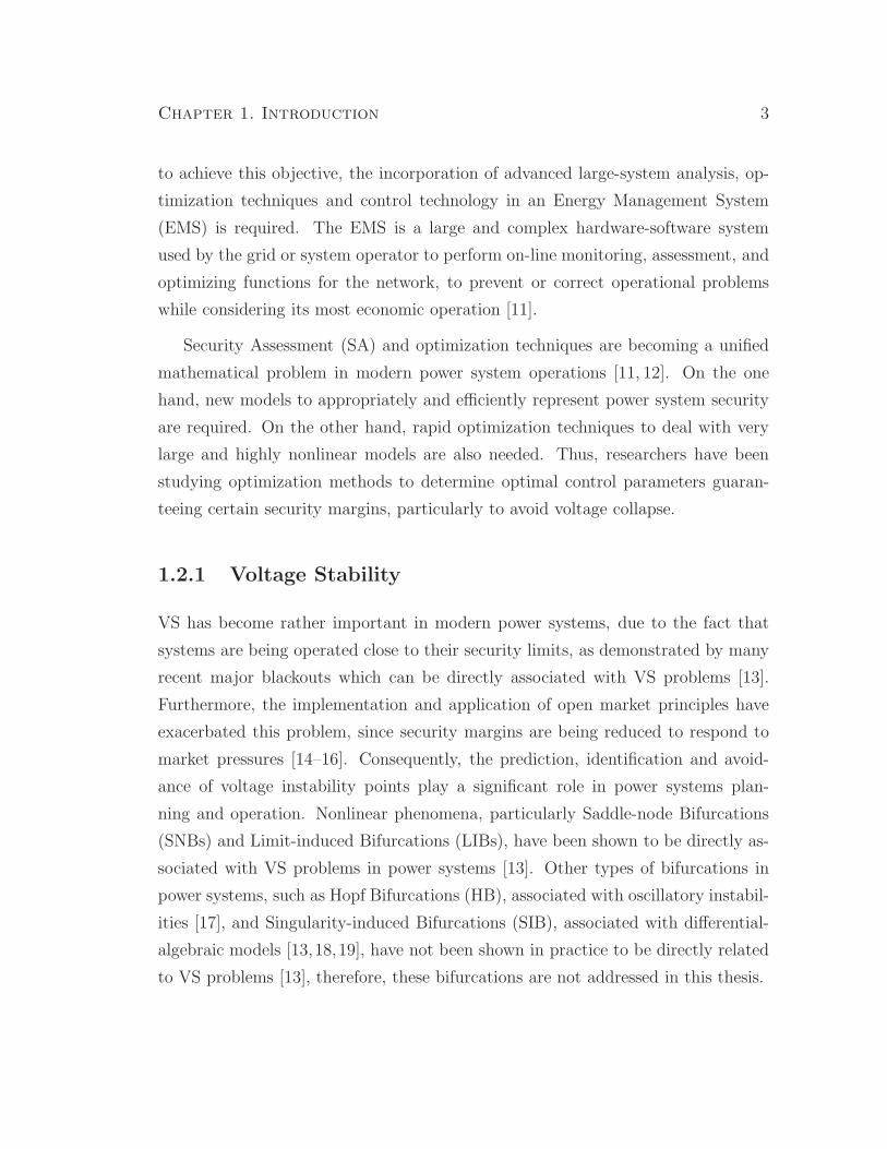
1.2.1 Voltage Stability
VS has become rather important in modern power systems, due to the fact that
systems are being operated close to their security limits, as demonstrated by many
recent major blackouts which can be directly associated with VS problems [13].
Furthermore, the implementation and application of open market principles have
exacerbated this problem, since security margins are being reduced to respond to
market pressures [14–16]. Consequently, the prediction, identification and avoid-
ance of voltage instability points play a significant role in power systems plan-
ning and operation. Nonlinear phenomena, particularly Saddle-node Bifurcations
(SNBs) and Limit-induced Bifurcations (LIBs), have been shown to be directly as-
sociated with VS problems in power systems [13]. Other types of bifurcations in
power systems, such as Hopf Bifurcations (HB), associated with oscillatory instabil-
ities [17], and Singularity-induced Bifurcations (SIB), associated with differential-
algebraic models [13,18,19], have not been shown in practice to be directly related
to VS problems [13], therefore, these bifurcations are not addressed in this thesis.
Chapter 1. Introduction 4
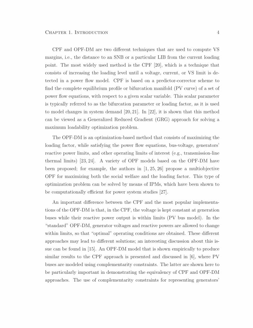
CPF and OPF-DM are two different techniques that are used to compute VS
margins, i.e., the distance to an SNB or a particular LIB from the current loading
point. The most widely used method is the CPF [20], which is a technique that
consists of increasing the loading level until a voltage, current, or VS limit is de-
tected in a power flow model. CPF is based on a predictor-corrector scheme to
find the complete equilibrium profile or bifurcation manifold (PV curve) of a set of
power flow equations, with respect to a given scalar variable. This scalar parameter
is typically referred to as the bifurcation parameter or loading factor, as it is used
to model changes in system demand [20, 21]. In [22], it is shown that this method
can be viewed as a Generalized Reduced Gradient (GRG) approach for solving a
maximum loadability optimization problem.
The OPF-DM is an optimization-based method that consists of maximizing the
loading factor, while satisfying the power flow equations, bus-voltage, generators’
reactive power limits, and other operating limits of interest (e.g., transmission-line
thermal limits) [23, 24]. A variety of OPF models based on the OPF-DM have
been proposed; for example, the authors in [1, 25, 26] propose a multiobjective
OPF for maximizing both the social welfare and the loading factor. This type of
optimization problem can be solved by means of IPMs, which have been shown to
be computationally efficient for power system studies [27].
An important difference between the CPF and the most popular implementa-
tions of the OPF-DM is that, in the CPF, the voltage is kept constant at generation
buses while their reactive power output is within limits (PV bus model). In the
“standard” OPF-DM, generator voltages and reactive powers are allowed to change
within limits, so that “optimal” operating conditions are obtained. These different
approaches may lead to different solutions; an interesting discussion about this is-
sue can be found in [15]. An OPF-DM model that is shown empirically to produce
similar results to the CPF approach is presented and discussed in [6], where PV
buses are modeled using complementarity constraints. The latter are shown here to
be particularly important in demonstrating the equivalency of CPF and OPF-DM
approaches. The use of complementarity constraints for representing generators’

Chapter 1. Introduction 5
limits is also discussed in [5], where an interesting analysis of the loadability sur-
face of a power system is presented. This thesis presents a detailed theoretical
analysis of the OPF-DM, demonstrating its “equivalency” with CPF approaches.
1.2.2 OPF-based Auction Models
OPFs have become one of the most widely used market tools in the electricity
industry, particularly in planning, real-time operation, and electricity market auc-
tions. New challenges have arisen with the introduction of competitive market
principles in electricity markets that have pushed power systems to be operated
closer to their stability limits in order to respond to market pressures. One of
these challenges is the proper representation of power system security in traditional
OPF-based auction models to guarantee reliable operations at reasonable electric-
ity prices. Furthermore, with the lack of investment in and development of new
transmission lines, and the increase in power transactions in a competitive elec-
tricity market, these challenges have become more relevant for market and system
operators.
The objective of the present research is to develop OPF-based auction mod-
els that are computationally robust and can properly represent system security,
so that these can be used in a market/system operating environment [12, 28, 29].
Thus, different approaches to represent system security limits in the OPF-based
auction models have been proposed in the literature [30–34], so that the optimal
solution guarantees a secure power dispatch. These OPFs have evolved from “clas-
sical” optimization models with simple lower and upper bounds in some of the
operating constraints (e.g., bus voltage and reactive power limits [35]), to more
sophisticated models such as the VSC-OPFs, which incorporate highly nonlinear
constraints derived from traditional VS analysis (e.g., [34]).
The OPF models which look for optimal control settings in the pre-contingency
state to prevent violations in the post-contingency state are commonly referred to
as SC-OPFs [36]. An example of a SC-OPF model can be found in [35], where the
Chapter 1. Introduction 6
authors propose an OPF iterative technique that searches for secure voltage levels,
which meet the bus voltage and reactive power limits after any single outage. The
authors in [37, 38] put emphasis on secure generation schedules to prevent trans-
mission lines from overloading. The authors in [39] propose the use of line outage
distribution factors to formulate contingency constraints in the SC-OPF. An inter-
esting approach of a linear SC-OPF, which includes bus voltage magnitudes and
reactive power, is proposed in [40]; the model is formulated using graph theory. The
main disadvantage of these models is that the operating constraints are calculated
off-line; therefore, these constraints may impose a more restrictive operative region
that does not necessarily reflect actual security levels, yielding improper market sig-
nals [1, 41]. Furthermore, the condition of voltage collapse is not well represented
in any of these models.
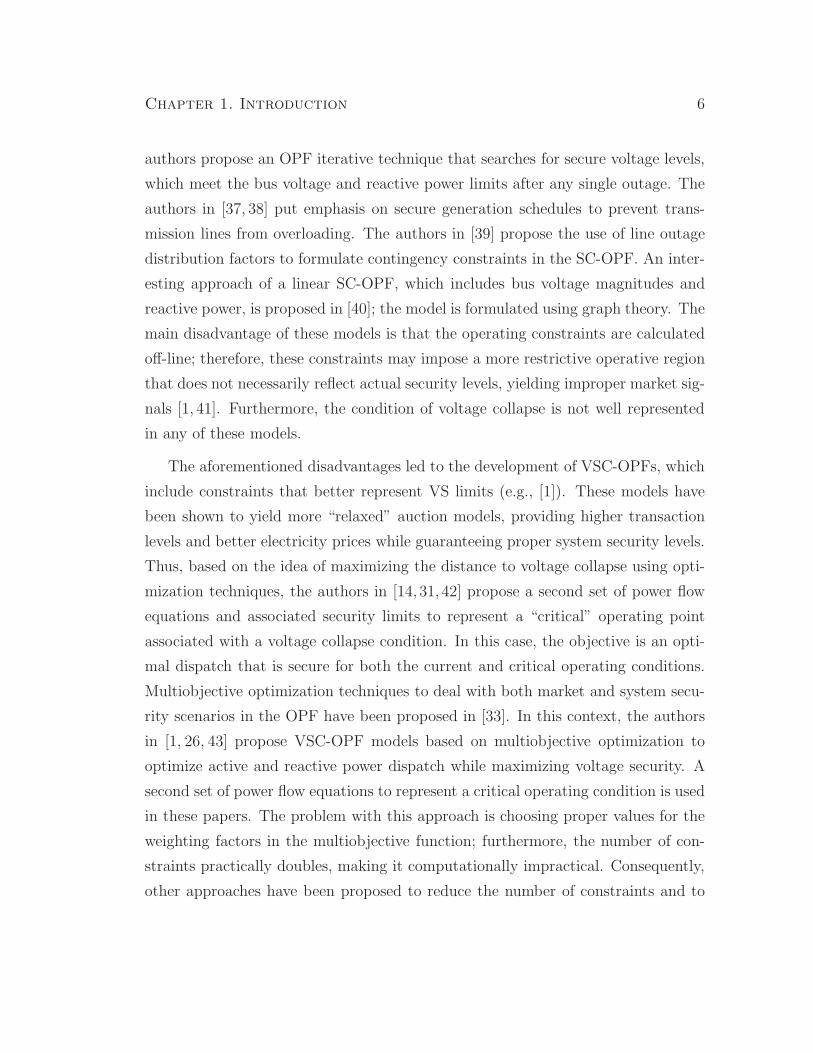
The aforementioned disadvantages led to the development of VSC-OPFs, which
include constraints that better represent VS limits (e.g., [1]). These models have
been shown to yield more “relaxed” auction models, providing higher transaction
levels and better electricity prices while guaranteeing proper system security levels.
Thus, based on the idea of maximizing the distance to voltage collapse using opti-
mization techniques, the authors in [14, 31, 42] propose a second set of power flow
equations and associated security limits to represent a “critical” operating point
associated with a voltage collapse condition. In this case, the objective is an opti-
mal dispatch that is secure for both the current and critical operating conditions.
Multiobjective optimization techniques to deal with both market and system secu-
rity scenarios in the OPF have been proposed in [33]. In this context, the authors
in [1, 26, 43] propose VSC-OPF models based on multiobjective optimization to
optimize active and reactive power dispatch while maximizing voltage security. A
second set of power flow equations to represent a critical operating condition is used
in these papers. The problem with this approach is choosing proper values for the
weighting factors in the multiobjective function; furthermore, the number of con-
straints practically doubles, making it computationally impractical. Consequently,
other approaches have been proposed to reduce the number of constraints and to

Chapter 1. Introduction 7
make them more practical. One method consist of the use of VS indices (VSI) to
represent proximity to voltage collapse in the OPF. Most of the proposed indices
are based upon small perturbations in the load, loading margins, or the monitoring
of some variables whose deviations at the collapse point can be predicted, such as
the Available Transfer Capability (ATC), tangent vector indices, or reactive power
indices [23, 30, 44–52].
The use of the minimum singular value (MSV) of the power flow Jacobian has
been also proposed as a VSI for VS assessment [44, 45], since this index tends to
become zero at the voltage collapse point. Thus, the authors in [34,53] incorporate
this index into the OPF as a VS constraint to guarantee a minimum distance to
voltage collapse. Approximate derivatives are required during the solution process
of this VSC-OPF, however, which may lead to convergence problems. The main
disadvantage of available VSC-OPF models is that they present significant com-
putational problems, which render them impractical. This thesis focuses on this
particular issue by proposing novel solution techniques, so that VSC-OPFs can be
better applied in practice.
1.3 Objectives
The following are the main objectives of this thesis, concentrating on the application
of optimization techniques to VS analysis, and on the development of practical
methods to solve VSC-OPFs:
1. Demonstrate that a solution of the OPF-DM correspond to either an SNB or
LIB point of a power flow model.
2. Propose practical solution methods to solve a MSV-based VSC-OPF, so that
it can be applied to more “realistic” systems.
3. Implement and test the proposed VSC-OPF solution technique using “stan-
dard” mathematical optimization tools.

Chapter 1. Introduction 8
4. Study the possible application of SDP to solve the VSC-OPF.
1.4 Thesis Outline
This thesis is organized into six chapters and one appendix as follows:
Chapter 2 presents a review of the main concepts of VS analysis and optimiza-
tion techniques of interest in this thesis. It describes the models used in nonlinear
theory for the characterization of VS in bifurcation analysis. Then, a brief intro-
duction to power systems security assessment is presented, followed by a discussion
of the most recently proposed VSC-OPF-based auction models. This chapter also
summarizes the primal-dual IPM, and the basis of SDP.
Chapter 3 presents a comprehensive theoretical study of the OPF-DM. This
work consist of reordering the the Karush-Kuhn-Tucker (KKT) conditions for op-
timality at the solution of the OPF-DM, so that the transversality conditions for
SNB and LIB in bifurcation theory can be derived. The analytical results are fur-
ther illustrated with numerical examples that show this optimization method yields
equivalent maximum loading points as the CPF.
Chapter 4 describes the development of a solution technique for the MSV-based
VSC-OPF, which is based on the SVD of the power flow Jacobian, plus an iterative
solution process. The proposed model and solution technique is tested using two
realistic test systems and compared with both a previously proposed method and
a SC-OPF.
Chapter 5 presents an optimization method based on the primal-dual IPM and
cutting planes (CP) to solve the MSV-based VSC-OPF. The proposed solution
technique is first described, and then several simulations are carried out to study
its performance. This is followed by numerical examples and a comparison with
the proposed technique in Chapter 4. Finally, it presents an analysis of the possible
application of SDP to the solution of the same VSC-OPF model.

Chapter 1. Introduction 9
Chapter 6 summarizes the conclusions and main contributions of this thesis, as
well as discusses possible future work.
Finally, Appendix A presents a brief description of the test systems, and provides
the data of the test systems.

Chapter 2
Background Review
2.1 Introduction
This chapter presents a review of the concepts, models, and tools related to the
research work presented in this thesis. It first discusses the modeling and analysis
of VS, using bifurcation theory, and also the tools used for VS assessment, as well
as the use of these concepts and tools for power system security analysis. The
most recent SC-OPFs and VSC-OPFs models are also discussed here, highlighting
advantages and disadvantages of each one. The primal-dual IPM algorithm, and
SDP are summarized in this chapter as well.
2.2 Voltage Stability Analysis
Voltage stability is associated with the capability of a power system to maintain
steady acceptable voltages at all buses, not only under normal operating conditions,
but also after being subjected to a disturbance [54]. It is a well established fact
that voltage collapse in power systems is associated with system demand increasing
beyond certain limits, as well as with the lack of reactive power support in the
10

Chapter 2. Background Review 11
system caused by limitations in the generation or transmission of reactive power.
System contingencies such as generator or unexpected line outages exacerbate, if
not trigger, the VS problems [13, 55]. Usually, VS analysis consists of determining
the system conditions at which the equilibrium points of a dynamic model of the
power system merge and disappear; these points have been associated with certain
bifurcations of the corresponding system models [13].
Voltage stability is an important problem in modern power systems due to
the catastrophic consequences of this phenomena. Thus, determining the largest
possible margin to the point of voltage collapse is becoming an essential part of
new electricity markets. These markets are also seeking ways to reduce operating
costs; as a matter of fact the application of open market principles has resulted
in stability margins being reduced to respond to market pressures [14, 15]. In an
open electricity market, voltage security requirements are typically associated with
transmission congestion and its associated high prices [16].
2.2.1 Effects of Increasing Demand
A slow increase in the system demand, such as that due to normal daily load
variations, can have negative effects on VS. If any small increase in loading demand
occurs, the reactive power demand will be greater than supply, and the voltage will
decrease. As the voltage decreases, the difference between reactive power supply
and demand increases, and the voltage falls even more until it eventually falls to a
very small value. This phenomenon is generally known as voltage collapse. The two
terms of voltage collapse are total voltage collapse and partial voltage collapse. The
former means that the collapse in permanent; the latter is used when the voltage is
below some technical acceptable limit and does not correspond to system instability
but an emergency state [56].
It is well-known that an excess of reactive power results in voltage increase,
while a deficit of reactive power results in a voltage decrease. Thus, consider the
equilibrium point s shown in Figure 2.1. If one assumes that there is small negative

Chapter 2. Background Review 12
Q
u
s
Q (V)L
Q (V)S
DV
DV
Vu V
s
Figure 2.1: QS(V ) and QL(V ) characteristics and equilibrium points
voltage disturbance ∆V , the reactive power supply QS(V ) would be greater than the
reactive power demand QL(V ). This excess of reactive power tends to increase the
voltage until it returns to point s. If the disturbance produces an increase in voltage,
the resulting deficit in reactive power will force the voltage to decrease and return
to point s. Thus, one can conclude that the equilibrium point s is stable. If one now
considers the equilibrium point u under the same small negative disturbance, the
reduction in voltage will produce a deficit of reactive power with QS(V ) < QL(V ),
which will produce a further decrease in voltage. As a result of both the voltage and
reactive power being reduced, the voltage will not recover; therefore, the equilibrium
point u is unstable [56]. Notice that if the QL(V ) characteristic is lifted upward,
the equilibrium points u and s tend to move toward each other until they eventually
merge and disappear, which is a phenomenon explained using bifurcation theory as
explained below.

Chapter 2. Background Review 13
2.2.2 System Models
Power systems are typically modeled with nonlinear differential-algebraic equations
(DAE), which are a class of nonlinear systems, as follows:[
x
0
]=
[f(x, y, λ, p)
g(x, y, λ, p)
]= F (z, λ, p) (2.1)
where x ∈ Rnx is a vector of state variables that represents the dynamic states
of generators, loads, and system controllers; y ∈ Rny is a vector of algebraic vari-
ables that typically results from neglecting fast dynamics, such as load bus voltages
magnitudes and angles; z = (x, y) ∈ Rnz ; λ ∈ R
+ stands for a slow varying “uncon-
trollable” parameter, typically used to represent load changes that move the system
from one equilibrium point to another; and p ∈ Rnp represents “controllable” pa-
rameters associated with control settings, such as Automatic Voltage Regulator
(AVR) set points. The function f : Rnx × R
ny × R+ × R
np 7→ Rnx is a nonlinear
vector field directly associated with the state variables x, and representing the sys-
tem differential equations, such as those associated with the generator mechanical
dynamics; and g : Rnx × R
ny × R+ × R
np 7→ Rny represents the system nonlinear
algebraic constraints, such as the power flow equations, and algebraic constraints
associated with the synchronous machine model.
If the Jacobian ∇Ty g(·) of the algebraic constraints is invertible, i.e., nonsingular
along a “solution path” of (2.1), the behavior of the system is mainly defined by
the following Ordinary Differential Equation (ODE) model
x = f(x, y−1(x, λ, p), λ, p)
where y−1(x, λ, p) results from applying the Implicit Function Theorem to the al-
gebraic constraints along the system trajectories of interest [22,57]. The interested
reader is referred to [58] for a detailed discussion when ∇Ty g(·) is not guaranteed
to be invertible. This problem is associated with SIBs, which go beyond the scope
of this thesis, since this phenomenon is not directly related to VS problems in
practice [13].
Chapter 2. Background Review 14
Equilibrium points zo = (xo, yo) of (2.1) are defined by the solutions of the
nonlinear equations:
F (zo, λo, po) =
[f(xo, yo, λo, po)
g(xo, yo, λo, po)
]= 0
It is important to highlight the fact that the system equilibria are in practice
obtained from a subset of equations:
G(zo, λo, po) = G|o = 0 ⊂ F (zo, λo, po) = F |o = 0 (2.2)
where G|o = 0 stands for the power flow equations; G ⊂ g; zo ∈ Rnz ⊂ z is the
set of voltage and angles at all buses as well as the reactive power of the generator
(PV) buses; and po ∈ Rnp ⊆ p usually represents the voltage levels and “base”
active power injections at PV buses, “base” active and reactive power injections at
load buses, transformer fixed-tap settings and other controller settings.
Power flow models have been used in practice for VS assessment, since these
models form the basis for defining the actual system operating conditions [13].
However, one should be aware that the solutions of the power flow equations do
not necessarily correspond to system equilibria, since a solution of G|o = 0 does
not imply that F |o = 0; however, in practice, this issue tends to be ignored.
2.2.3 Bifurcation Analysis
Bifurcation theory yields concepts and tools to classify, study, and give qualitative
and quantitative information about the behavior of a nonlinear system close to
bifurcation or “critical” equilibrium points as system parameters change [59]. The
parameters are assumed to change “slowly”, so that the system can be assumed to
“move” from equilibrium point to equilibrium point by these changes (quasi-static
assumption). Hence, bifurcation analysis is usually associated with the study of
equilibria of the nonlinear system model [13].
Chapter 2. Background Review 15
In power systems, SNBs and some types of LIBs are basically characterized
by the local merging and disappearance of power flow solutions as certain system
parameters, particularly system demand, slowly change; this phenomena has been
associated with VS problems [13]. These kinds of bifurcations are also referred to
in the technical literature as fold or turning points.
Saddle-node Bifurcations
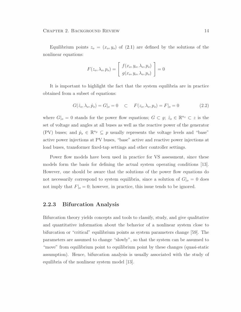
These types of codimension-1 (single parameter), generic bifurcations occur when
two equilibrium points, one stable and one unstable in practice, merge and disap-
pear as the parameter λ slowly changes, as illustrated in the PV curves of Figures 2.2
and 2.3. In these figures, VGiand QGi
stand for a generator i’s terminal voltage
magnitude and reactive power, respectively. Mathematically, the SNB point for
the power flow model (2.2) is a solution point (zc, λc, po) where the Jacobian ∇Tz G|c
has a simple zero eigenvalue, with nonzero eigenvectors [60, 61]. The following
transversality conditions can be used to characterize and detect SNBs [22]:
∇Tz G|cv = ∇zG|cw = 0 (2.3)
∇λG|c w 6= 0 (2.4)
wT[∇2T
z G|cv]v 6= 0 (2.5)
where v and w ∈ Rnz are unique normalized right and left eigenvectors of the
Jacobian ∇Tz G|c. The first condition implies that the Jacobian matrix is singular;
the second and third conditions ensure that there are no equilibria near (zc, λc, po)
for λ > λc (or λ < λc, depending on the sign of (2.5)). Note that the subscript c is
used throughout this thesis to denote a bifurcation point.
Limit-induced Bifurcations
These types of codimension-1 (single parameter), generic bifurcations in power sys-
tems were first studied in detail in [62], and can be typically encountered in these
Chapter 2. Background Review 16
Stable points
SNB
Unstable points
VGi= VGoi
QGi< QGimax
VLoi
Voltage
λ λc
Figure 2.2: SNB without QG limits.
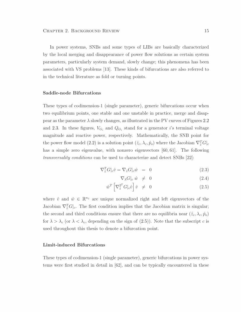
Actuation RegimeLIDB
QGimax
SNB
Saturation Regime
VGi< VGoi
QGi= QGimax
VGoi
Voltage
λ λc
Figure 2.3: Stable limit point (LIDB) followed by a SNB.
Chapter 2. Background Review 17
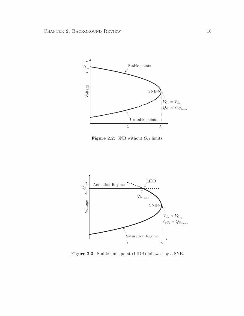
Actuation RegimeLISB
VGi= VGoi
QGi= QGimax
Saturation Regime
VGoi
Voltage
λ λc
Figure 2.4: Unstable limit point (LISB).
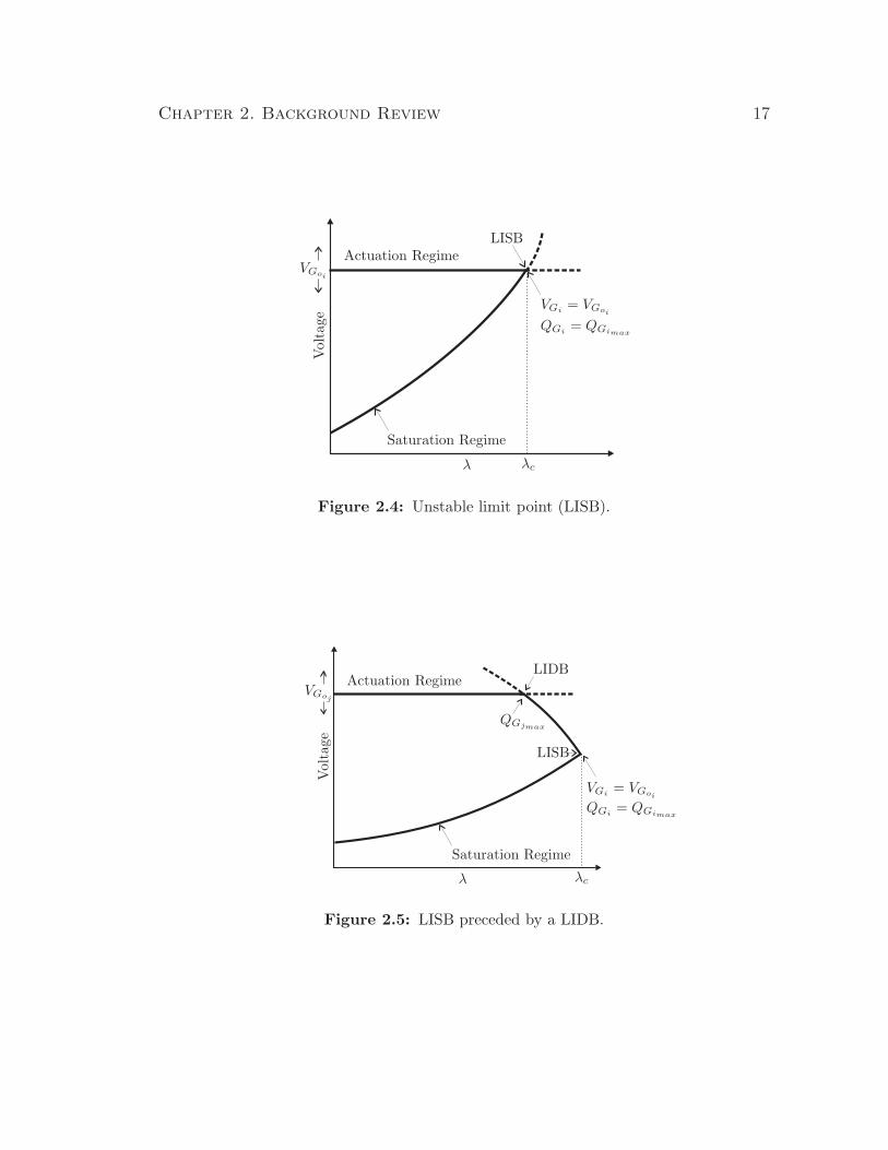
Actuation RegimeLIDB
QGjmax
LISB
Saturation Regime
VGi= VGoi
QGi= QGimax
VGoj
Voltage
λ λc
Figure 2.5: LISB preceded by a LIDB.
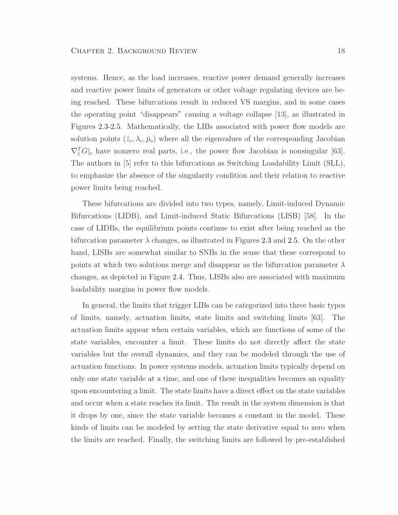
Chapter 2. Background Review 18
systems. Hence, as the load increases, reactive power demand generally increases
and reactive power limits of generators or other voltage regulating devices are be-
ing reached. These bifurcations result in reduced VS margins, and in some cases
the operating point “disappears” causing a voltage collapse [13], as illustrated in
Figures 2.3-2.5. Mathematically, the LIBs associated with power flow models are
solution points (zc, λc, po) where all the eigenvalues of the corresponding Jacobian
∇Tz G|c have nonzero real parts, i.e., the power flow Jacobian is nonsingular [63].
The authors in [5] refer to this bifurcations as Switching Loadability Limit (SLL),
to emphasize the absence of the singularity condition and their relation to reactive
power limits being reached.
These bifurcations are divided into two types, namely, Limit-induced Dynamic
Bifurcations (LIDB), and Limit-induced Static Bifurcations (LISB) [58]. In the
case of LIDBs, the equilibrium points continue to exist after being reached as the
bifurcation parameter λ changes, as illustrated in Figures 2.3 and 2.5. On the other
hand, LISBs are somewhat similar to SNBs in the sense that these correspond to
points at which two solutions merge and disappear as the bifurcation parameter λ
changes, as depicted in Figure 2.4. Thus, LISBs also are associated with maximum
loadability margins in power flow models.
In general, the limits that trigger LIBs can be categorized into three basic types
of limits, namely, actuation limits, state limits and switching limits [63]. The
actuation limits appear when certain variables, which are functions of some of the
state variables, encounter a limit. These limits do not directly affect the state
variables but the overall dynamics, and they can be modeled through the use of
actuation functions. In power systems models, actuation limits typically depend on
only one state variable at a time, and one of these inequalities becomes an equality
upon encountering a limit. The state limits have a direct effect on the state variables
and occur when a state reaches its limit. The result in the system dimension is that
it drops by one, since the state variable becomes a constant in the model. These
kinds of limits can be modeled by setting the state derivative equal to zero when
the limits are reached. Finally, the switching limits are followed by pre-established
Chapter 2. Background Review 19
actions (e.g., relaying mechanisms or protective limiters in the physical system),
which might result in a change in the whole system, and consequently in the states.
These limits can be modeled, for instance, by introducing certain binary variables
that represent the internal logic of a relay element.
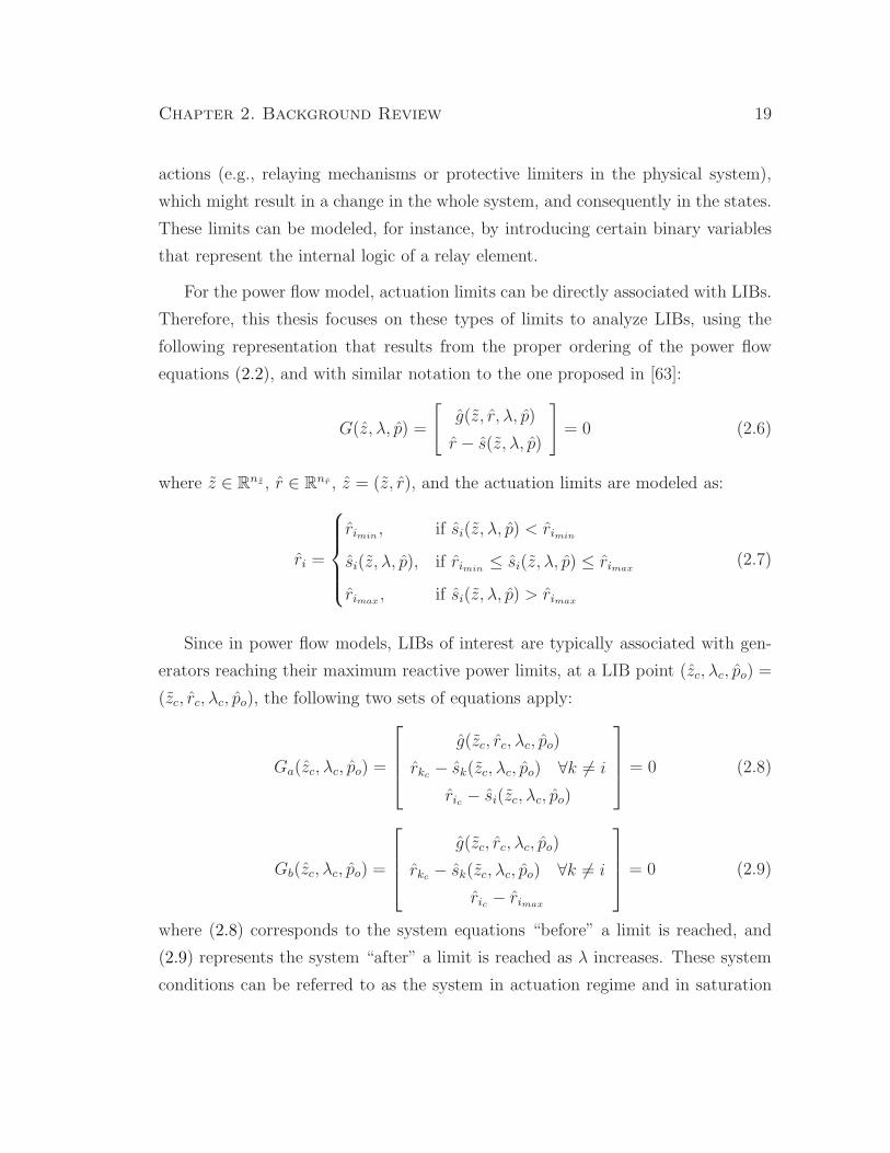
For the power flow model, actuation limits can be directly associated with LIBs.
Therefore, this thesis focuses on these types of limits to analyze LIBs, using the
following representation that results from the proper ordering of the power flow
equations (2.2), and with similar notation to the one proposed in [63]:
G(z, λ, p) =
[g(z, r, λ, p)
r − s(z, λ, p)
]= 0 (2.6)
where z ∈ Rnz , r ∈ R
nr , z = (z, r), and the actuation limits are modeled as:
ri =
rimin, if si(z, λ, p) < rimin
si(z, λ, p), if rimin≤ si(z, λ, p) ≤ rimax
rimax , if si(z, λ, p) > rimax
(2.7)
Since in power flow models, LIBs of interest are typically associated with gen-
erators reaching their maximum reactive power limits, at a LIB point (zc, λc, po) =
(zc, rc, λc, po), the following two sets of equations apply:
Ga(zc, λc, po) =
g(zc, rc, λc, po)
rkc − sk(zc, λc, po) ∀k 6= i
ric − si(zc, λc, po)
= 0 (2.8)
Gb(zc, λc, po) =
g(zc, rc, λc, po)
rkc − sk(zc, λc, po) ∀k 6= i
ric − rimax
= 0 (2.9)
where (2.8) corresponds to the system equations “before” a limit is reached, and
(2.9) represents the system “after” a limit is reached as λ increases. These system
conditions can be referred to as the system in actuation regime and in saturation
Chapter 2. Background Review 20
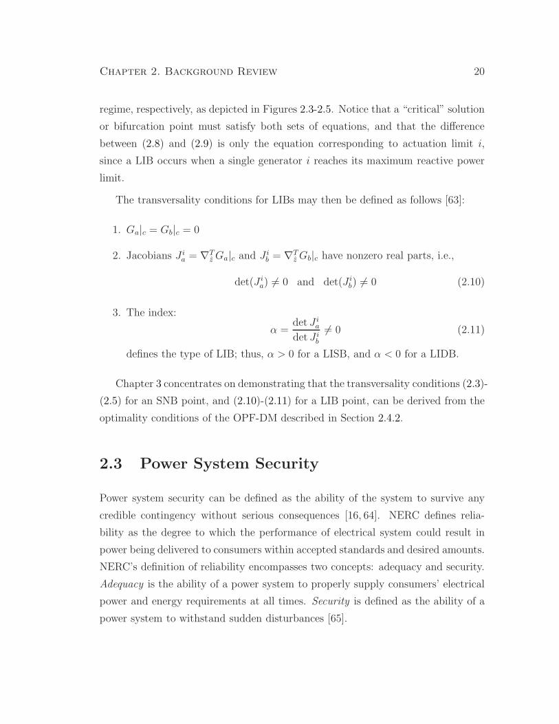
regime, respectively, as depicted in Figures 2.3-2.5. Notice that a “critical” solution
or bifurcation point must satisfy both sets of equations, and that the difference
between (2.8) and (2.9) is only the equation corresponding to actuation limit i,
since a LIB occurs when a single generator i reaches its maximum reactive power
limit.
The transversality conditions for LIBs may then be defined as follows [63]:
1. Ga|c = Gb|c = 0
2. Jacobians J ia = ∇T
z Ga|c and J ib = ∇T
z Gb|c have nonzero real parts, i.e.,
det(J ia) 6= 0 and det(J i
b) 6= 0 (2.10)
3. The index:
α =det J i
a
det J ib
6= 0 (2.11)
defines the type of LIB; thus, α > 0 for a LISB, and α < 0 for a LIDB.
Chapter 3 concentrates on demonstrating that the transversality conditions (2.3)-
(2.5) for an SNB point, and (2.10)-(2.11) for a LIB point, can be derived from the
optimality conditions of the OPF-DM described in Section 2.4.2.
2.3 Power System Security
Power system security can be defined as the ability of the system to survive any
credible contingency without serious consequences [16, 64]. NERC defines relia-
bility as the degree to which the performance of electrical system could result in
power being delivered to consumers within accepted standards and desired amounts.
NERC’s definition of reliability encompasses two concepts: adequacy and security.
Adequacy is the ability of a power system to properly supply consumers’ electrical
power and energy requirements at all times. Security is defined as the ability of a
power system to withstand sudden disturbances [65].
Chapter 2. Background Review 21
System security is composed of three major functions that are carried out in a
control center:
1. System Monitoring: Provides the operators of the power system with up-to-
date information on the conditions on the power system.
2. Contingency Analysis: The results of this analysis allow systems to be oper-
ated defensively.
3. SC-OPF: A contingency analysis is combined with an OPF, so that no con-
tingencies result in limit violations. A SC-OPF model is discussed in detail
in Section 2.5.2.
Transmission-line failures cause changes in the flows and voltages on transmis-
sion equipment remaining connected to the system. Therefore, the analysis of
transmission failures requires methods to predict these flows and voltages so as
to be sure they are within their respective limits. One way to gain speed in the
solution of a contingency analysis procedure is to use an approximate model of
the power system. For many systems, the use of DC load flow models provides
adequate capability. In such systems, the voltage magnitudes may not be of great
concern, and hence the DC load flow provides sufficient accuracy with respect to
the megawatt flows. For other systems, when voltage is a concern, a full AC load
flow analysis is required [36].
2.3.1 Security Assessment
Security Assessment is the process by which the power system static security level
is determined, by means of detecting limit violations in its pre-contingency or post-
contingency operating states [11, 64]. The first function in this process is violation
detection in the actual operating state (e.g., monitoring actual flows or voltage
limits). The second is contingency analysis, which identifies potential emergency

Chapter 2. Background Review 22
operating states, through iterative simulations on the power system in the context
of what would happen if certain outages occur [11,64]. The second function implies
several difficulties in practice; for instance, how to handle the power system, de-
termine which contingency scenarios are more likely to happen, and speed up the
process, since the solution of many contingency cases requires a significant compu-
tational effort. In the same manner, the determination of the VS margin consists
of finding how much the system can be stressed in a particular load direction from
its current operating state and yet remain secure [16].
Two alternative definitions of SA exist, namely, direct and indirect. In direct
SA, the objective is to estimate the probability of the power system changing from
the normal state to the emergency state. In indirect SA, one defines the system
“security” variables that must be maintained within limits to provide adequate
reserve margins [64].
2.3.2 Available Transfer Capability
The ATC is defined as “a measure of the transfer capability remaining in the phys-
ical transmission network for further commercial activity over and above already
committed uses”. Mathematically, ATC is defined as [66]:
ATC = TTC - TRM - ETC
where:
• Total Transfer Capability (TTC): Is the maximum loading level of the system
considering an N-1 contingency criterion. The TTC is defined as:
TTC = min{PmaxIlim
, PmaxVlim
, PmaxSlim} (2.12)
where Ilim, Vlim and Slim represent the thermal, voltage magnitude, and sta-
bility limits, respectively [67].

Chapter 2. Background Review 23
ETC ATC
TRM
TTC
Operating Point
Slim
Vlim
Ilim
Slim
Normal
Worst contingency (N-1)
Volt
age
lc Power (l)l00
Figure 2.6: ATC evaluation with dominant voltage limits.
• Transmission Reliability Margin (TRM): This measure considers uncertainty
to account for other contingencies; it is usually assumed to be a fixed value
(e.g., WECC’s 5% of TTC). The authors in [68], propose a formula that cal-
culates the TRM based on a probabilistic approach for various uncertainties.
• Existing Transmission Commitments (ETC): Basically, represents the current
loading level.
• Capacity Benefit Margin (CBM): is a reserve made by load-serving entities to
guarantee access to generation from different interconnected systems to meet
their generation reliability requirements [69]. This could be considered to be
included in the ETC.
2.3.3 Loading Margin
The maximum loading margin can be defined as the distance between a given op-
erating point and a maximum loading condition reached in a particular pattern of

Chapter 2. Background Review 24
load increase. This margin is the most basic and widely accepted index of voltage
collapse [13]. Mathematically, the loading margin for a typical power flow model is
defined as follows:
λ = λc − λo
where λc is the maximum loading of the system at a given limit, either the bus
voltage limit (Vlim), thermal limit (Ilim), or VS limit (Slim), which corresponds to
an SNB or LIB point in the PV curve of a power flow model [67], and λo stands for
the base or current operating point. The parameter λ typically represents variations
in load and generation schedules as follows:
PG = PGo + (λ + KG)PS (2.13)
PL = PLo + λPD (2.14)
QL = QLo + λKLPD (2.15)
where PGo , PLo and QLo stand for the “base” generation and load levels, thus
defining an “initial” operating point; KG is a variable used to represent a distributed
slack bus; and KL is a parameter used to represent a load with a constant power
factor. PS and PD are used here to define the generation and load “directions”,
respectively, needed to compute loading margins and PV curves. All loads are
typically assumed to have constant power factors.
Figure 2.6 depicts the computation of ATC based on the loading margin in terms
of PV curve typically used in VS studies [13]. In this analysis, system stability is
assumed to be represented by VS margins, which is an adequate approximation,
since blackouts are typically associated with VS problems. The “external” PV
curve corresponds to the system under normal operating conditions and assuming
certain dispatch, whereas the “internal” PV curve is the system under the worst
single contingency for the assumed system conditions. Observe that the voltage
limits in this example are assumed to define the lowest loading level corresponding
to the TTC. The current operating point defines the ETC (and CBM), any point
before the ATC is considered a “safe” operating point, and the TRM is a small
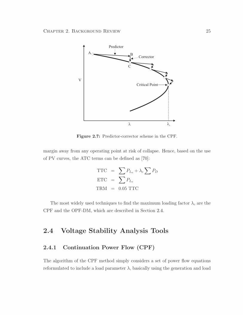
Chapter 2. Background Review 25
V
A B
C
l lc
Predictor
Critical Point
Corrector
Figure 2.7: Predictor-corrector scheme in the CPF.
margin away from any operating point at risk of collapse. Hence, based on the use
of PV curves, the ATC terms can be defined as [70]:
TTC =∑
PLo + λc
∑PD
ETC =∑
PLo
TRM = 0.05 TTC
The most widely used techniques to find the maximum loading factor λc are the
CPF and the OPF-DM, which are described in Section 2.4.
2.4 Voltage Stability Analysis Tools
2.4.1 Continuation Power Flow (CPF)
The algorithm of the CPF method simply considers a set of power flow equations
reformulated to include a load parameter λ, basically using the generation and load
Chapter 2. Background Review 26
directions shown in (2.13)-(2.15). The power flow model in this technique is solved
for automatic changes in λ using a predictor-corrector scheme that remains well-
conditioned at and around the critical point, i.e., the maximum loadability point
λc.
Figure 2.7 illustrates the iterative process of a typical CPF technique. The al-
gorithm starts from a known solution A which corresponds to a power flow solution
at the current loading point. Then, it uses a tangent predictor to estimate a so-
lution B corresponding to an increased value of the load parameter, and it finally
uses a “corrector” to find the exact solution C using a classical Newton-Raphson
technique [20]. This method allows one to trace the voltage profile of a power
flow model, also known as an equilibrium profile or bifurcation manifold. Hence, it
allows for the calculation of security indices such as the ATC.
The advantage of this method is that additional information regarding the be-
havior of some system variables can be obtained during the solution process. This
information, then, can be used as indices to predict proximity to a voltage collapse.
However, although this algorithm is very robust, it is computationally expensive,
especially for large systems with multiple limits [71].
UWPFLOW is a CPF research tool that allows one to trace PV curves and
calculate λc values [72]. This tool is used in this thesis to obtain all the PV curves
and VSI.
2.4.2 OPF-based Direct Method (OPF-DM)
Optimization methods can be used to compute maximum loadability points of
power flow models, which are directly associated with SNBs and LISBs of the
corresponding model equations, as initially proposed in [23]. Thus, based on the
SNB and LIB definitions presented in Section 2.2.3, the bifurcation point directly
corresponds to the solution of the following optimization model, as formally demon-
Chapter 2. Background Review 27
strated in Section 3.2:
maxz,r,λ
λ (2.16a)
s.t. g(z, r, λ, po) = 0 (2.16b)
h(z, r, λ, po) = 0 (2.16c)
rmin ≤ r ≤ rmax (2.16d)
where the nonlinear function h is used to represent the actuation limit equations
introduced in (2.6), since in these optimization models the actuation limits are typ-
ically not represented explicitly, as illustrated below. The issue of how constraints
(2.16c) are actually represented in this model, and the effect of this modeling on
the solution of the optimization problem (2.16) is discussed in detail below. Note
that (2.16d) basically corresponds to (2.7).
OPF-DM in Standard Form
For a typical power flow model, let z = (δ, VL, KG), r = (QG, VG), and p = (PS, PD).
In this case, δ stands for all the bus voltage phasor angles but one (slack bus);
VL and VG correspond to the load and generator bus voltage phasor magnitudes,
respectively, and QG represents the generator reactive power output. The variables
PS and PD define the change in power generation and demand, as shown in (2.13)-
(2.15).
Based on the aforementioned variable definition and if the actuation functions
(2.16c) are omitted, the model can be restated as:
maxδ,VL,KGQG,VG,λ
λ (2.17a)
s.t. G(δ, VL, KG, QG, VG, λ, PS, PD) = 0 (2.17b)
QGimin≤ QGi
≤ QGimax∀i ∈ G (2.17c)
VGimin≤ VGi
≤ VGimax∀i ∈ G (2.17d)
Chapter 2. Background Review 28
where G stand for the classical active and reactive power balanced equations for
each generator and load bus (two for every system bus), as defined in (2.6), i.e.,
PGi− PLi
− Gp(δ, VL, VG, Gij, Bij) = 0 ∀i ∈ B (2.18)
QGi−QL
i− Gq(δ, VL, VG, Gij, Bij) = 0 ∀i ∈ B (2.19)
PGi, PLi
, and QLiare defined in (2.13)-(2.15); Gij and Bij are the real and imaginary
part of the bus admittance matrix, respectively; G is the set of indices of generating
units; and B is the set of indices of network buses. Observe that G ⊂ G in (2.2),
since G contains some additional equations representing limits as per (2.6). It is
also important to highlight the fact that in this optimization model no other limits
such as load bus voltage magnitude limits, generator active power limits, or power
transfer limits, which are typical operating limits considered in such OPF models,
are represented here. The reason for this is that these are “hard” limits and not
actuation limits, i.e., limits that basically define “undesirable” operating conditions
which may be associated with system protections rather than system controls, and
hence do not lead to LIBs. These limits would only clutter the theoretical analyzes
presented in Chapter 3, without adding much to the discussions.
It has been shown that if no limits become active, the sufficient KKT opti-
mality conditions evaluated at the solution point of (2.17) are equivalent to the
transversality conditions (2.3) and (2.4) for SNBs [22]. However, it has not yet
been formally shown that the third transversality condition (2.5) will also be met,
which is an issue addressed in Chapter 3. It can also be argued that this model
may provide a maximum loading point different from that obtained using the CPF
technique if reactive power limits become active [6]. This is due to the fact that the
objective of the optimization model (2.17) is to “optimize” the generator voltage
and reactive power levels so that the loading factor is maximized. Hence, there is no
guarantee that the voltage at generation buses would be maintained at a constant
level while the reactive power output at such buses is within its limits. This is the
typical representation of the generator voltage regulation controls in the power flow
models used in CPF techniques.
Chapter 2. Background Review 29
If limits are considered, and the parameters PS and PD are free to change, the
problem is transformed into an optimal active and reactive dispatch problem for
the maximization of the loading margin. Indeed, other optimization problems can
be derived from this concept, such as the maximization of the social welfare while
ensuring a loading margin, as discussed in Section 2.5.2.
OPF-DM with Complementarity Constraints
An optimization model that has been empirically shown to yield the same SNB
or LISB points as a CPF technique has been proposed in [6]. The authors in this
paper propose an optimization model that is based upon the idea that many prob-
lems encountered in engineering, physics, or economics, which behave according to
different rules under different circumstances, can be modeled using complementar-
ity constraints because these constraints can be used to model a change in system
behavior. Thus, the change from a PV to a PQ bus, when a generation reactive
power limit is reached can be modeled using these type of constraints in the OPF
problem as follows [73]:
0 ≤ (QGk−QGkmin
) ⊥ Vak≥ 0
⇒ (QGk–QGkmin
)Vak= 0
0 ≤ (QGkmax−QGk
) ⊥ Vbk≥ 0
⇒ (QGk−QGkmax
)Vbk= 0
where Va and Vb are auxiliary, nonnegative variables that allow increasing or de-
creasing the generator voltage set point, depending on the state of QG. Thus:
if QGk= QGkmin
⇒ Vak≥ 0 and Vbk
= 0
if QGkmin< QGk
< QGkmax⇒ Vak
= Vbk= 0
if QGk= QGkmax
⇒ Vak= 0 and Vbk
≥ 0
Chapter 2. Background Review 30
This yields the following Mixed Complementarity Problem (MCP) [6]:
maxδ,VL,KGQG,VG,λ
λ (2.20a)
s.t. G(δ, VL, KG, QG, VG, λ, PS, PD) = 0 (2.20b)
(QGk−QGkmin
)Vak= 0 ∀k ∈ G (2.20c)
(QGk−QGkmax
)Vbk= 0 ∀k ∈ G (2.20d)
VGk= VGko
+ Vak− Vbk
∀k ∈ G (2.20e)
QGkmin≤ QGk
≤ QGkmax∀k ∈ G (2.20f)
Vak, Vbk
≥ 0 ∀k ∈ G (2.20g)
where VGo is the generator voltage regulator set point, i.e., the generator termi-
nal voltage level if QG, is within limits; and the constraints (2.20c)-(2.20e), asso-
ciated with the auxiliary variables Va and Vb, are used to model the actuation
limits associated with the generator voltage regulators. Hence, in this model,
z = (δ, VL, KG, VG), r = (QG, Va, Vb), p = (PS, PD, VGo), and g and h are con-
tained within constraints (2.20b)-(2.20e). The actual representation of these two
vector functions is discussed in detail in Section 3.2.
2.5 Optimal Power Flow Models with Security
Constraints
An independent system operator has to deal with the market participants by re-
ceiving their bids and offers, so that it can accommodate the necessary transactions
to balance supply and demand while maintaining power system security. Typically,
the system operator accomplishes these objectives through a cost minimization pro-
cess based on an OPF. This section briefly discusses the most recent OPF models
that include security constraints.
The first model represents system security by imposing limits on the transmis-
sion system power flows. The second makes use of a multiobjective optimization

Chapter 2. Background Review 31
technique and a second set of power flow equations to represent system security,
whereas the third model uses the MSV of a power flow Jacobian to represent VS.
2.5.1 Security-Constrained OPF (SC-OPF)
The following optimization model, typically referred to as an SC-OPF, corresponds
to a single-period auction model; the objective function in this case is social welfare,
to ensure that generators maximize their income from power production, while loads
minimize the prices paid for their power demand:
maxδ,VL,QG
VG,PS ,PD
∑
j∈D
CDjPDj−∑
i∈G
CSiPSi
(2.21a)
s.t G(δ, VL, QG, VG, PS, PD) = 0 (2.21b)
PSimin≤ PSi
≤ PSimax∀i ∈ G (2.21c)
PDjmin≤ PDj
≤ PDjmax∀j ∈ D (2.21d)
QGimin≤ QGi
≤ QGimax∀i ∈ G (2.21e)
Vimin≤ Vi ≤ Vimax ∀i ∈ B (2.21f)
Iij(δ, V ) ≤ Iijmax ∀(i, j) ∈ T , i 6= j (2.21g)
Pij(δ, V ) ≤ Pijmax ∀(i, j) ∈ T , i 6= j (2.21h)
Here CS and CD are the cost functions; PSminand PSmax represent the minimum
and maximum power output limits of the generators’ bid power; PDminand PDmax
represent the minimum and maximum power limits of demand bid blocks; and
Iij(δ, V ) represents the current in the transmission element between buses i and
j. The function Pij(δ, V ) is used to represent transmission system security limits,
which are determined off-line by means of stability and contingency studies, in order
to represent security limits in the auction model. Finally, D is the set of indices of
loads, and T is the set of indices of transmission lines and transformers.
It is important to highlight that the stability limits Pijmax used in this model are
computed off-line using possible dispatch scenarios that do not necessarily represent
Chapter 2. Background Review 32
the actual system conditions [1, 43]. Thus, VSC-OPF models have been proposed
to better represent system security by means of including additional constraints,
such as the MSV of the power flow Jacobian, as described in the following section.
2.5.2 Voltage-Stability-Constrained OPF (VSC-OPF)
Multiobjective VSC-OPF
A technique for representing system security in the operation of decentralized elec-
tricity markets, with special emphasis on VS, is proposed in [1]. In this case, the
proposed optimization model is:
maxPS ,PD,λc,QGc
QG,V,Vc,δ,δc,kGc
w1
(∑
j∈D
CDjPDj−∑
i∈G
CSiPSi
)+ w2λc (2.22a)
s.t. G(δ, V, KG, QG, PS, PD) = 0 (2.22b)
Gc(δc, Vc, KG, QGc , λc, PS, PD) = 0 (2.22c)
λcmin≤ λc ≤ λcmax (2.22d)
PSimin≤ PSi
≤ PSimax∀i ∈ G (2.22e)
PDjmin≤ PDj
≤ PDjmax∀j ∈ D (2.22f)
QGimin≤ QGi
≤ QGimax∀i ∈ G (2.22g)
QGimin≤ QGci
≤ QGimax∀i ∈ G (2.22h)
Vimin≤ Vi ≤ Vimax ∀i ∈ B (2.22i)
Vimin≤ Vci
≤ Vimax ∀i ∈ B (2.22j)
Pij(δ, V ) ≤ Pijmax ∀(i, j) ∈ T i 6= j (2.22k)
Pij(δc, Vc) ≤ Pijmax ∀(i, j) ∈ T i 6= j (2.22l)
This model accounts for the system security by including a second set of power flow
equations, reactive power and voltage limits at the critical condition associated with
the maximum loading point λc, hence the subscript c. The maximum or critical
loading point could be either associated with a thermal or bus voltage limit, or a VS

Chapter 2. Background Review 33
limit corresponding to a system singularity SNB or LISB. The loading margin λc
is free to change between certain limits which ensures a minimum level of security,
while the upper limit defines a maximum required level of security.
The multiobjective function (2.22a) is composed of two terms weighted by two
factors w1 > 0 and w2 > 0. The first term represents the social welfare, whereas
the second term ensures that the distance between the market solution and the
critical point is maximized [1]. The disadvantage of this formulation is that the
solution will depend on the value of the weighting factors, leading to “improper”
market signals. Notice that w1 must be greater than zero, otherwise there would
be no representation of the social welfare, and if w2 is zero, λc does not necessarily
represent a maximum loading condition. To link the social welfare and the max-
imum loading condition, the author in [74] defines w1 = (1 − w) and w2 = w for
0 < w < 1.
In this model, the generator and load powers at the current and maximum
loading condition are defined as follows:
PG = PGo + PS PGc = (1 + λc + KG)PG
PL = PLo + PD PLc = (1 + λc)PL
(2.23)
where KG in this case is used to distribute the system losses associated with the
power flow equations that represent the critical conditions, in proportion to the
value of PS obtained in the solution process.
A similar VSC-OPF model that considerers an N-1 contingency criterion is
proposed in [74]. The model is essentially the same as the one shown in (2.22); the
main difference is that contingencies are included by taking out selected lines when
formulating the power flow equations at the critical point (2.22c). By doing this, it
is ensured that the current solution of the VSC-OPF problem is also feasible for the
worst single contingency. Similar OPF approaches are proposed in [14, 31, 41, 42].
The disadvantages of this model are as follows: the number of constraints in-
creases considerably; the difficulty of choosing adequate values for the weighting
Chapter 2. Background Review 34
factors; and the presence of the loading margin in the objective function. This final
disadvantage leads to not having pure market signals.
A mixed CPF-OPF technique based on sensitivities obtained from the OPF
Lagrangian multipliers is proposed in [32]. The sensitivities are used to approxi-
mate the power directions for the CPF method in order to calculate the loading
parameter based upon an N-1 contingency criterion. This technique has important
advantages over previous work proposed by the authors in [1], since the multi-
objective optimization is no longer used because of the drawback of dealing with
weighting factors, and not providing pure market solutions. However, the compu-
tational effort is still a problem.
MSV-based VSC-OPF
A model to improve the representation of VS margins in the OPF has been pro-
posed in [34, 53]. The resulting VSC-OPF market clearing and power dispatch
optimization model is defined as follows:
maxδ,VL,QG
VG,PS ,PD
∑
j∈D
CDjPDj−∑
i∈G
CSiPSi
(2.24a)
s.t G(δ, VL, QG, VG, PS, PD) = 0 (2.24b)
σmin{J} ≥ σc (2.24c)
PSimin≤ PSi
≤ PSimax∀i ∈ G (2.24d)
PDjmin≤ PDj
≤ PDjmax∀j ∈ D (2.24e)
QGimin≤ QGi
≤ QGimax∀i ∈ G (2.24f)
Vimin≤ Vi ≤ Vimax ∀i ∈ B (2.24g)
Iij(δ, V ) ≤ Iijmax ∀(i, j) ∈ T , i 6= j (2.24h)
where J is the power flow Jacobian of the system at a power flow solution point,
and σmin is the MSV of J . This model is basically the same as the SC-OPF, except
for the transmission system limits on Pij , which are implicitly represented in the VS
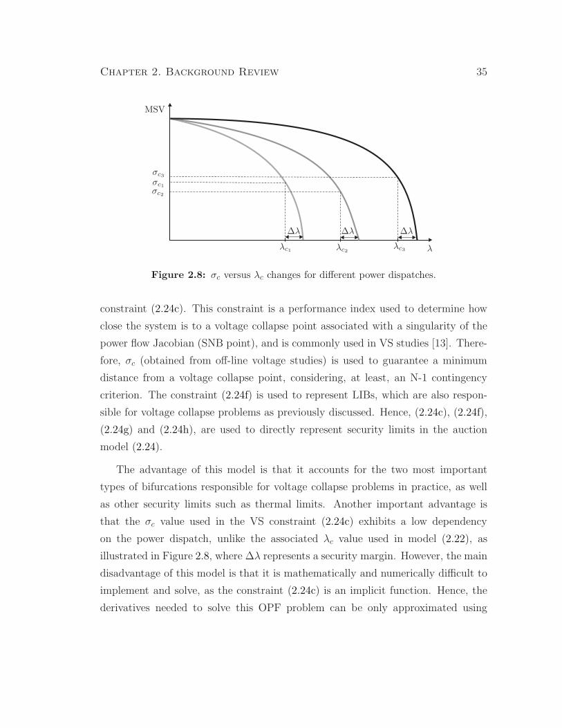
Chapter 2. Background Review 35
σc2
σc1
σc3
∆λ∆λ∆λ
λc1 λc2λc3 λ
MSV
Figure 2.8: σc versus λc changes for different power dispatches.
constraint (2.24c). This constraint is a performance index used to determine how
close the system is to a voltage collapse point associated with a singularity of the
power flow Jacobian (SNB point), and is commonly used in VS studies [13]. There-
fore, σc (obtained from off-line voltage studies) is used to guarantee a minimum
distance from a voltage collapse point, considering, at least, an N-1 contingency
criterion. The constraint (2.24f) is used to represent LIBs, which are also respon-
sible for voltage collapse problems as previously discussed. Hence, (2.24c), (2.24f),
(2.24g) and (2.24h), are used to directly represent security limits in the auction
model (2.24).
The advantage of this model is that it accounts for the two most important
types of bifurcations responsible for voltage collapse problems in practice, as well
as other security limits such as thermal limits. Another important advantage is
that the σc value used in the VS constraint (2.24c) exhibits a low dependency
on the power dispatch, unlike the associated λc value used in model (2.22), as
illustrated in Figure 2.8, where ∆λ represents a security margin. However, the main
disadvantage of this model is that it is mathematically and numerically difficult to
implement and solve, as the constraint (2.24c) is an implicit function. Hence, the
derivatives needed to solve this OPF problem can be only approximated using

Chapter 2. Background Review 36
interval formulas that may lead to convergence problems [34], since the MSV can
behave in a rather nonlinear way [13]. As a result, this constraint becomes a
“soft” constraint, and it may not guarantee an accurate solution in some cases,
as demonstrated in Section 4.3. Furthermore, current mathematical programming
languages and large-scale solvers available for nonlinear optimization cannot be
used for its implementation and solution, since these are not able to handle this
type of implicit function constraint.
The aforementioned drawbacks are what motivates the development of the prac-
tical solution method for this particular VSC-OPF model. The proposed solution
method, which is described and analyzed in detail in Chapter 4, concentrates on
the practical reformulation of constraint (2.24c).
2.5.3 Locational Marginal Prices (LMP)
The theory of spot pricing states that the spot market price must reflect the inter-
action of supply and demand. Thus, the price in a competitive market is set by
the highest cost supplier when there is enough supply, and by the marginal (low-
est value) demand [75]. In this context, a central operator receives voluntary bids
from market participants, assuming that the submitted bids reflects true marginal
costs1 of production and marginal benefits2 of consumption. The operator then
finds an optimal operating state by means of a cost minimization process, which
is based on an OPF. The solution must satisfy all the transmission constraints,
balance of power, and minimum cost, and must provide the Locational Marginal
Prices (LMPs), which are basically the Lagrange multipliers of the OPF, as shown
below. The LMPs differ by location because energy is cheaper to produce in some
locations, and the transmission line capacity is limited. For this reason, locational
pricing of energy is also called congestion pricing [77, 78].
1The change in total cost that results from a unit increase in output. It is calculated as the
increase in total cost divided by the increase in output [76].2The extra benefit received from a small increase in the consumption of a good or service. It
is calculated as the increase in total benefit divided by the increase in consumption [76].

Chapter 2. Background Review 37
Consider the following standard OPF model:
minδ,VL,QG
VG,PS ,PD
∑
i∈G
CSiPSi−∑
j∈D
CDjPDj
(2.25a)
s.t G(δ, VL, QG, VG, PS, PD) = 0 (2.25b)
0 ≤ PSi≤ PSimax
∀i ∈ G (2.25c)
0 ≤ PDj≤ PDjmax
∀j ∈ D (2.25d)
QGimin≤ QGi
≤ QGimax∀i ∈ G (2.25e)
Vimin≤ Vi ≤ Vimax ∀i ∈ B (2.25f)
Pij(δ, V ) ≤ Pijmax ∀(i, j) ∈ T , i 6= j (2.25g)
which can be restated as the following Lagrangian function using a logarithmic
barrier IPM approach:
min L =∑
i∈G CSiPSi−∑
j∈D CDjPDj
−µTGG(δ, VL, KG, QG, VG, PS, PD)
−µTPSmax
(PSmax − PS − sPSmax)
−µTPDmax
(PDmax − PD − sPDmax)
−µTQGmax
(QGmax −QG − sQGmax)
−µTQGmin
(QG −QGmin− sQGmin
)
−µTVmax
(Vmax − V − sVmax)
−µTVmin
(V − Vmin − sVmin)
−µPijmax(Pijmax − Pijmax − sPijmax
)
−µs(∑
i ln si)
(2.26)
where [µT
GµT
PSmaxµT
PDmaxµT
QGmaxµT
QGminµT
VmaxµT
VminµT
PijmaxµT
s ] > 0 is a vector of La-
grange multipliers, and [sTPSmax
sTPDmax
sTQGmax
sTQGmin
sTVmax
sTVmin
sTPijmax
] ≥ 0 is a vec-
tor of slack variables. Thus, the marginal cost for supply and demand can be
defined as [41]:
∂L∂PSi
= CSi− µ
GSi+ µPSimax
(2.27)
∂L∂PDi
= −CDi+ µ
GDi+ µPDimax
(2.28)
Chapter 2. Background Review 38
as ∂Gi
∂PSi= 1 and ∂Gi
∂PDi= −1, and where µG = [µT
GSµT
GDµT
GQ]. Thus, from (2.27)
and (2.28), the LMP or shadow price for each market participant is given by the
corresponding Lagrange multiplier [79]:
LMPi =
µ
GSi
µGDi
(2.29)
Furthermore, conditions (2.27) and (2.28) set the suppliers’ and consumers’ op-
eration conditions, so that their marginal cost and marginal benefit match the
corresponding market price [77].
It is well-known that as the loading level increases, the stability margin de-
creases, and some control actions have to be taken; however, this might result in
increased operating cost. Hence, the associated cost of such actions can be consid-
ered as the operational cost of improving system security [26] [42].
2.6 Optimization Methods
2.6.1 Primal-Dual Interior-Point Method (IPM)
Optimality Conditions
In general, the OPF problem is a non-linear programming (NLP) problem that is
used to determine the “optimal” control parameter settings to minimize a desired
objective function, subject to certain system constraints [42]. An OPF can be
generally represented as follows:
minχ
F (χ) (2.30a)
s.t. G(χ) = 0 (2.30b)
H ≤ H(χ) ≤ H (2.30c)
χ ≤ χ ≤ χ (2.30d)
Chapter 2. Background Review 39
where F (χ) : Rnχ → R is the objective function, e.g, the social welfare in (2.21a)
or the loading factor λ; G(χ) : Rnχ → R
m generally represents the power flow
equations (G); and H(χ) : Rnχ → R
p can represent transmission line limits, voltage
or reactive power, with lower and upper limits represented by H and H , respectively.
The vector of system variables χ ∈ Rnχ typically includes voltage magnitudes and
angles, active and reactive power levels, or control variables; their lower and upper
limits are represented by χ and χ, respectively.
Thus, assume that F (χ), G(χ) and H(χ) are twice continuously differentiable.
The first step to state the optimality conditions is to transform the inequality
constraints into equality constraints by adding slack variables. The slack variables
are handled implicitly by incorporating them into the objective function using a
logarithmic barrier term, imposing strict positivity on the slack variables as follows:
min F (χ)− µk
p∑
i=1
(ln ιi + ln κi) (2.31a)
s.t G(χ) = 0 (2.31b)
−ι− κ + H −H = 0 (2.31c)
−H(χ)− κ + H = 0 (2.31d)
ι > 0, κ > 0 (2.31e)
where ι ∈ Rp and κ ∈ R
p are slack variables. The Lagrangian function Lµ(φ) is
then stated as follows:
Lµ(φ) = F (χ)− µk
P∑
i=1
(ln ιi + ln κi)
− ρT G(χ)− βT(−ι− κ + H −H
)− γT
(−H(χ)− κ + H
)(2.32)
where φ = [ιT κT βT γT χT ρT ]; ρ ∈ Rm, β ∈ R
p and γ ∈ Rp are the Lagrange
multipliers, also called dual variables. A local minimum of (2.32) satisfies the

Chapter 2. Background Review 40
following KKT optimality conditions:
∇φLµ(φ) =
∇ιLµ(φ)
∇κLµ(φ)
∇βLµ(φ)
∇γLµ(φ)
∇χLµ(φ)
∇ρLµ(φ)
=
Θβ − µke
Λ − µke
ι + κ−H + H
H(χ) + κ−H
∇χF (χ)− JG(χ)T ρ + JH(χ)T γ
−G(χ)
= 0 (2.33)
where Θ = diag(ι1, ι2, ..., ιp); Λ = diag(κ1, κ2, ..., κp); e = [1 1 ... 1]T ; = γ + β;
∇χF : Rnχ → R
nχ is the gradient of F (χ); JG : Rnχ → R
m×nχ is the Jacobian of
G(χ); and JH : Rnχ → R
p×nχ is the Jacobian of H(χ).
The third, fourth and sixth terms in (2.33) along with (ι, κ) ≥ 0 ensure primal
feasibility. The fifth term along with (β, ) ≥ 0 ensures dual feasibility, and the
first and second terms are the µ-complementarity conditions.
Primal-dual Interior-Point Method Algorithm
The primal-dual IPM algorithm, is based on Newton’s method to solve nonlinear
equations. Figure 2.9 shows the algorithm’s flow chart, and the steps are described
below.
Computing Newton Directions
The solution of the KKT optimality conditions with Newton’s method leads to the
following indefinite system of equations parameterized by µk, which are used to
compute the Newton direction at every iteration:
[Jo −JT
G
−JG 0
][∆χ
∆ρ
]=
[ϕx
ϕρ
](2.34)
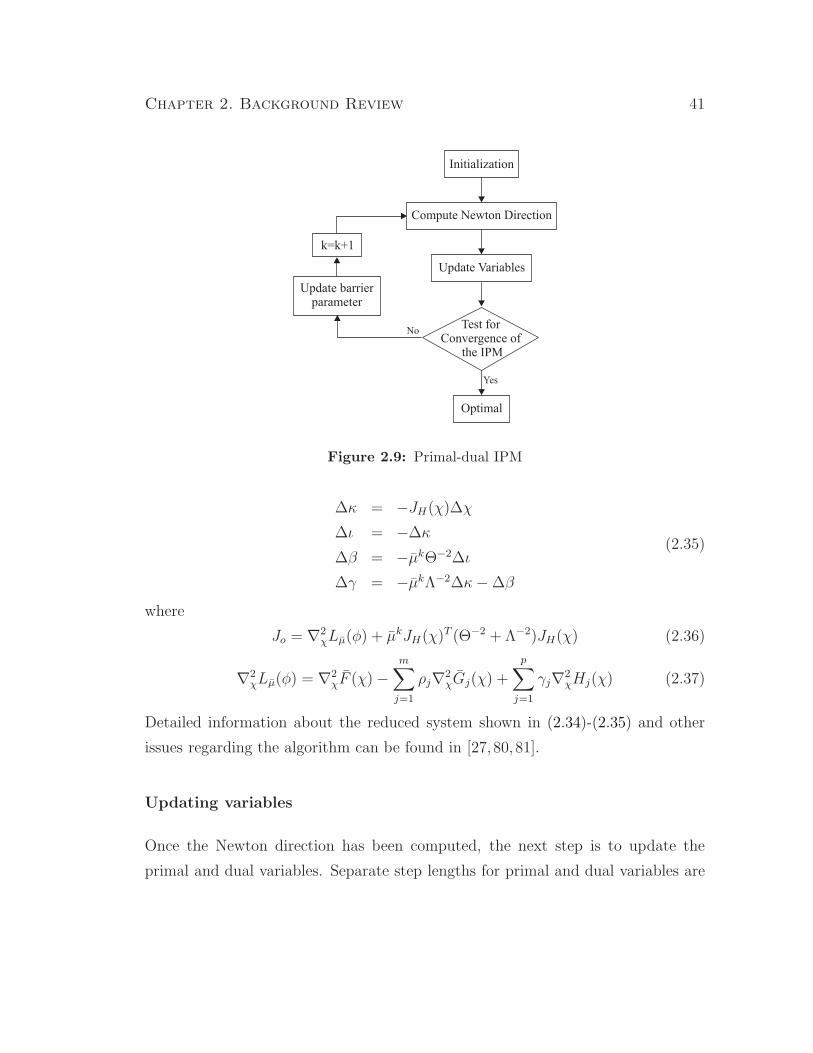
Chapter 2. Background Review 41
Initialization
Compute Newton Direction
Update Variables
Test forConvergence of
the IPM
Update barrierparameter
Optimal
k=k+1
Yes
No
Figure 2.9: Primal-dual IPM
∆κ = −JH(χ)∆χ
∆ι = −∆κ
∆β = −µkΘ−2∆ι
∆γ = −µkΛ−2∆κ−∆β
(2.35)
where
Jo = ∇2χLµ(φ) + µkJH(χ)T (Θ−2 + Λ−2)JH(χ) (2.36)
∇2χLµ(φ) = ∇2
χF (χ)−m∑
j=1
ρj∇2χGj(χ) +
p∑
j=1
γj∇2χHj(χ) (2.37)
Detailed information about the reduced system shown in (2.34)-(2.35) and other
issues regarding the algorithm can be found in [27, 80, 81].
Updating variables
Once the Newton direction has been computed, the next step is to update the
primal and dual variables. Separate step lengths for primal and dual variables are
Chapter 2. Background Review 42
calculated as follows:
αkP = min
{1, γ min
i
{−ιki∆ιi
∣∣∣∆ιi < 0,−κk
i
∆κi
∣∣∣∆κi < 0
}}(2.38)
αkD = min
{1, γ min
i
{−βki
∆βi
∣∣∣∆βi < 0,−k
i
∆i
∣∣∣∆i < 0
}}(2.39)
where the scalars αkP ∈ (0, 1] and αk
D ∈ (0, 1] are the step length parameters; and
the scalar γ ∈ (0, 1] is a safety factor to ensure that the next point will satisfy the
strict positivity conditions (a typical value is γ = 0.99995). Thus, the variables are
updated as follows:
χk+1 = χk + αkP ∆χ ρk+1 = ρk + αk
D∆ρ
ιk+1 = ιk + αkP ∆ι βk+1 = βk + αk
D∆β
κk+1 = κk + αkP∆κ γk+1 = γk + αk
D∆γ
(2.40)
Testing for Convergence and Reducing the Barrier Parameter
The last step in the IPM algorithm is to test for convergence and reduce the barrier
parameter. The criterion to stop the iterative process is based on the primal (ξ1)
and dual (ξ2) feasibilities, as well as complementarity conditions (ξ3), to satisfy
certain tolerances. Thus, the residual of the complementarity conditions, called the
complementarity gap, is computed at the point φk from:
ζk = (ιk)T βk + (κk)T νk (2.41)
µk+1 = σkdir
ζk
2p(2.42)
where the parameter σkdir ∈ (0, 1] is called the centering parameter. If σk
dir = 1, it
defines a centering direction, and if σkdir = 0, it gives a pure Newton step, known as
the affine-scaling direction. In practice, to decide whether to improve centrality or
reduce µk, σkdir is computed using to the following heuristic:
σ0dir = 0.2 (2.43)
σkdir = max{0.99σk−1
dir , 0.1}
Chapter 2. Background Review 43
The algorithm is stopped when one of the two sets of the following conditions are
met:ξk1 ≤ ǫ1 µk ≤ ǫµ
ξk2 ≤ ǫ1 or ||∆χ||∞ ≤ ǫ2
ξk3 ≤ ǫ2 ||G(χk)||∞ ≤ ǫ1
ξk2 ≤ ǫ2 ξk
4 ≤ ǫ2
(2.44)
where
ξ1 = max{
max{H −H(χ)
}, max
{H(χ)−H
}, ||G(χ)||∞
}(2.45)
ξ2 =||∆χF (χ)− JG(χ)T ρ + JH(χ)T γ||∞
1 + ||χ||2 + ||ρ||2 + ||γ||2(2.46)
ξ3 =ζ
1 + ||χ||2(2.47)
ξ4 =F (χk)− F (χk−1)
1 + |F (χk)| (2.48)
Typical tolerances are ǫ1 = 10−4, ǫ2 = 10−2ǫ1, and ǫµ = 10−12.
Choosing an Initial Point
An important characteristic of the primal-dual IPM is that a strictly feasible point is
not mandatory, hence the usual denomination infeasible primal-dual interior-point
method. Nonetheless, (ι, κ) > 0 and (β, ) > 0 have to be satisfied at every point,
so the IPM starts from a point φ0 such that (ι0, κ0) > 0 and (β0, 0) > 0. Besides
the strict positivity conditions, a good starting point should also satisfy two other
conditions. First, the point should be well-centered, and second, the point should
not be “too unfeasible”; that is, the duality gap should not be too large [81].
In practice, IPMs perform better if some initialization heuristic is used. For the
OPF the following estimations are suggested in [27, 81]:
• Estimate χ as a flat start using the middle point between the upper and lower
limits for the bounded variables.

Chapter 2. Background Review 44
• The primal slack variables are initialized as follows:
ι0 = min{max{γH∆, H(χ0)−H}, (1− γ)H∆}κ0 = H∆ − ι0
where H∆ := H −H, and γ := 0.25.
• The initial dual variables β0 and γ0 are defined as:
β0 = µ0(Θ0)−1e,
γ0 = µ0(Λ0)−1e− β0
2.6.2 Semidefinite Programming (SDP)
In SDP one minimizes a linear function of a symmetric matrix X, subject to lin-
ear constraints on the entries in X, under the restriction that X must be positive
semidefinite. Such a constraint is nonlinear and nonsmooth, but convex, so SDP
problems are convex optimization problems. This is significant because, for con-
vex optimization problems, any local minimum is a global minimum. SDP unifies
several standard problems (e.g., linear programming) and finds many applications
in engineering and combinatorial optimization [82–84]. A SDP problem is an opti-
mization problem of the following form:
min C ·X (2.49a)
s.t Ai ·X = bi, i = 1, ..., m (2.49b)
X � 0 (2.49c)
where X ∈ Sn is the matrix variable, and Sn is the set of symmetric n×n matrices,
and C ∈ Sn is the matrix of coefficients of the objective function. X � 0 denotes
that X is positive semidefinite (PSD), and:
C ·X = trace(CX)

Chapter 2. Background Review 45
is the standard inner product in Sn. A matrix A ∈ Sn is said to be positive
semidefinite (PSD) if:
vT Av =
n∑
i=1
n∑
j=1
Aij vivj ≥ 0 ∀v ∈ Rn
It may be helpful to think of X � 0 as stating that each of the n eigenvalues
of X must be non-negative. This concept fosters the application of SDP to the
MSV-based VSC-OPF problem, since the power flow Jacobian tends to be either
singular or close to singularity at a voltage collapse point.
2.7 Summary
This chapter introduces power system security concepts and the basis of VS. Bifur-
cation theory definitions used to characterize the VS phenomena in power systems
are presented, as well as the techniques used to determine SNB and LIB points
of a power flow model. This chapter also discusses the OPF-DM, and the most
recently proposed VSC-OPFs market clearing and power dispatch models. Finally,
the primal-dual IPM for NLP, and a brief introduction to SDP is presented.
The concepts presented in this chapter are used throughout this thesis to study
and propose optimization-based techniques to better represent VS in OPF-based
auction models in competitive electricity markets.

Chapter 3
Analysis of the OPF-DM
3.1 Introduction
This chapter presents a detailed theoretical analysis of the application of OPF-DM
to the study of SNBs and LIBs in power systems. Previous works have formally
shown that optimization methods can be used to compute SNBs in power system
models, and that these methods are basically equivalent to more “classical” com-
putational approaches [22]. Also, some issues associated with the application of
OPF-DMs to the computation of LIBs are discussed in [85], and the structure of
the loadability surface is studied in [5] using similar optimization methods. In [86],
fold bifurcations are also studied using an optimization model. However, up to now,
to the author’s knowledge, the links between solutions of OPF-DMs and SNBs and
LIBs have not yet been dealt with in the technical literature as formally and sys-
tematically as is done here. Hence, this chapter concentrates on demonstrating that
solution points obtained from a given OPF-DM model correspond to either SNB or
LIB points; this is accomplished by showing that the optimality conditions of these
solution points yield the transversality conditions of the corresponding bifurcation
points. A simple but realistic test system example is used to numerically illustrate
the theoretical discussions presented here.
46
Chapter 3. Analysis of the OPF-DM 47
3.2 Theoretical Analysis of the OPF-DM
In this section, it is formally shown that a solution to the OPF-DM model (2.20)
corresponds to either an SNB or a LISB, by demonstrating that the transversality
conditions of the corresponding bifurcations are met, based on the necessary and
sufficient optimality conditions of the optimal solution. Only LIBs associated with
maximum reactive power limits are analyzed here, since VS problems in practice are
typically associated with generators reaching these limits as demand in the system
increases. Therefore, in this thesis, actual SNBs and LIBs (2.1) are assumed to
correspond to similar “bifurcation” points of the power flow equations. This is the
case in certain power system models [61,87]; thus, this chapter concentrates on the
analysis of SNBs and LIBs of (2.2).
The following assumptions are made for the statement of the theorems and
corollary presented next [88]:
• Regularity and strict complementarity conditions must be met at the optimal
point, i.e., there must not be degeneracy of the optimization problem at the
solution point.
• The constraints should be C2 and convex in a neighborhood of the optimal
solution.
These assumptions are referred to throughout the rest of the chapter as optimality
solution (OS) assumptions for convenience. It is important to highlight the fact that
there is no guarantee that all possible solutions of (2.20) would meet these OS as-
sumptions. If these conditions are not met, then the solution could not be classified
as an SNB or LIB point with certainty, as per the theorems proved below. However,
from numerical results reported in various papers (e.g., [6, 23]), where these types
of optimization problems are solved for a variety of small and large electrical power
systems, these solutions are shown to meet these assumptions [86]. This is due to
the fact that in nonlinear system theory, codimension-1 (single parameter) bifurca-
tions SNBs and LIBs are considered generic [59], i.e., they are expected in power
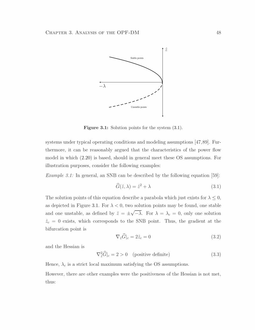
Chapter 3. Analysis of the OPF-DM 48
Stable points
Unstable points
−λ
z
Figure 3.1: Solution points for the system (3.1).
systems under typical operating conditions and modeling assumptions [47,89]. Fur-
thermore, it can be reasonably argued that the characteristics of the power flow
model in which (2.20) is based, should in general meet these OS assumptions. For
illustration purposes, consider the following examples:
Example 3.1: In general, an SNB can be described by the following equation [59]:
G(z, λ) = z2 + λ (3.1)
The solution points of this equation describe a parabola which just exists for λ ≤ 0,
as depicted in Figure 3.1. For λ < 0, two solution points may be found, one stable
and one unstable, as defined by z = ±√−λ. For λ = λc = 0, only one solution
zc = 0 exists, which corresponds to the SNB point. Thus, the gradient at the
bifurcation point is
∇zG|c = 2zc = 0 (3.2)
and the Hessian is
∇2zG|c = 2 > 0 (positive definite) (3.3)
Hence, λc is a strict local maximum satisfying the OS assumptions.
However, there are other examples were the positiveness of the Hessian is not met,
thus:
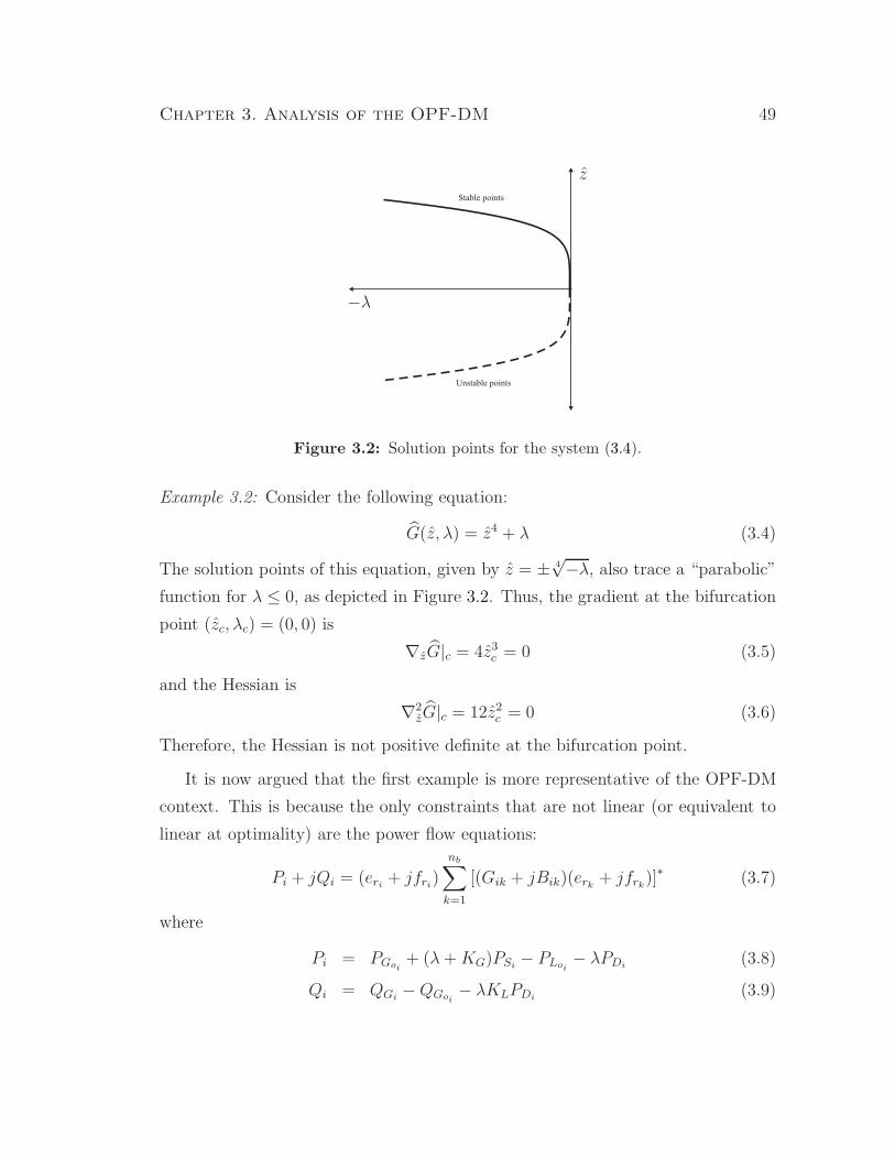
Chapter 3. Analysis of the OPF-DM 49
Stable points
Unstable points
−λ
z
Figure 3.2: Solution points for the system (3.4).
Example 3.2: Consider the following equation:
G(z, λ) = z4 + λ (3.4)
The solution points of this equation, given by z = ± 4√−λ, also trace a “parabolic”
function for λ ≤ 0, as depicted in Figure 3.2. Thus, the gradient at the bifurcation
point (zc, λc) = (0, 0) is
∇zG|c = 4z3c = 0 (3.5)
and the Hessian is
∇2zG|c = 12z2
c = 0 (3.6)
Therefore, the Hessian is not positive definite at the bifurcation point.
It is now argued that the first example is more representative of the OPF-DM
context. This is because the only constraints that are not linear (or equivalent to
linear at optimality) are the power flow equations:
Pi + jQi = (eri+ jfri
)
nb∑
k=1
[(Gik + jBik)(erk+ jfrk
)]∗ (3.7)
where
Pi = PGoi+ (λ + KG)PSi
− PLoi− λPDi
(3.8)
Qi = QGi−QGoi
− λKLPDi(3.9)
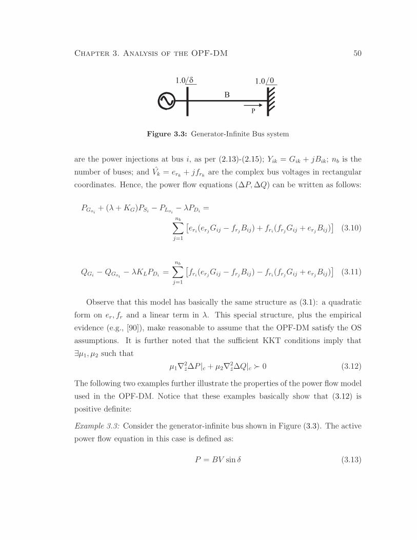
Chapter 3. Analysis of the OPF-DM 50
1.0
B
1.0d 0
P
Figure 3.3: Generator-Infinite Bus system
are the power injections at bus i, as per (2.13)-(2.15); Yik = Gik + jBik; nb is the
number of buses; and Vk = erk+ jfrk
are the complex bus voltages in rectangular
coordinates. Hence, the power flow equations (∆P, ∆Q) can be written as follows:
PGoi+ (λ + KG)PSi
− PLoi− λPDi
=nb∑
j=1
[eri
(erjGij − frj
Bij) + fri(frj
Gij + erjBij)
](3.10)
QGi− QGoi
− λKLPDi=
nb∑
j=1
[fri
(erjGij − frj
Bij)− fri(frj
Gij + erjBij)
](3.11)
Observe that this model has basically the same structure as (3.1): a quadratic
form on er, fr and a linear term in λ. This special structure, plus the empirical
evidence (e.g., [90]), make reasonable to assume that the OPF-DM satisfy the OS
assumptions. It is further noted that the sufficient KKT conditions imply that
∃µ1, µ2 such that
µ1∇2z∆P |c + µ2∇2
z∆Q|c ≻ 0 (3.12)
The following two examples further illustrate the properties of the power flow model
used in the OPF-DM. Notice that these examples basically show that (3.12) is
positive definite:
Example 3.3: Consider the generator-infinite bus shown in Figure (3.3). The active
power flow equation in this case is defined as:
P = BV sin δ (3.13)

Chapter 3. Analysis of the OPF-DM 51
since er = V cos δ and fr = V sin δ, it follows that:
P = BV sin δ ⇔ λ = Bfr (3.14)
The maximum loading point optimization problem here can be formulated as
follows:
miner,fr,λ
−λ (3.15a)
s.t. Bfr − λ = 0 (3.15b)
e2r + f 2
r − 1 = 0 (3.15c)
where (3.15c) is a constraint on the voltage magnitude at the generation bus. The
Lagrangian function can then be stated as:
L(er, fr, λ, µ1, µ2) = −λ + µ1(Bfr − λ) + µ2(e2r + f 2
r − 1) (3.16)
and the first-order KKT conditions are:
∇erL|c = 2ercµ2c = 0 (3.17)
∇frL|c = Bµ1c + 2frcµ2c = 0 (3.18)
∇λL|c = −µ1c − 1 = 0 (3.19)
∇µ1L|c = Bfrc − λc = 0 (3.20)
∇µ2L|c = e2
rc+ f 2
rc− 1 = 0 (3.21)
Thus, the optimal solution is:
erc
frc
λc
µ1c
µ2c
=
0
1
B
−1B2
(3.22)
On the other hand, the Hessian of the Lagrangian function can be written as follows:
∇2(er,fr ,λ)L =
2µ2 0 0
0 2µ2 0
0 0 0
(3.23)

Chapter 3. Analysis of the OPF-DM 52
1.0
B
V0 d
P+jK PL
Figure 3.4: Generator-Infinite Bus system
which evaluated at the optimal point yields:
∇2(er ,fr,λ)L|c =
B 0 0
0 B 0
0 0 0
(3.24)
Hence,
µ1c∇2(er,fr)(Bfr − λ)|c + µ2c∇2
(er,fr)(e2r + f 2
r − 1)|c ≻ 0 (3.25)
i.e.,
− 1
[0 0
0 0
]+
B
2
[2 0
0 2
]=
[B 0
0 B
]≻ 0 (3.26)
Example 3.4: Consider the generator-load bus shown in Figure 3.4. The active and
reactive power flow equations are defined in this case as:
P = −BV sin δ ⇔ −frB − λ = 0 (3.27)
KLP = −BV 2 + BV cos δ ⇔ −B(e2r + f 2
r ) + Ber −KLλ = 0 (3.28)
The maximum loading point can then be calculated as follows:
miner,fr,λ
−λ (3.29a)
s.t. −Bfr − λ = 0 (3.29b)
−B(e2r + f 2
r ) + Ber −KLλ = 0 (3.29c)
and the Lagrangian can be stated as:
L(er, fr, λ, µ1, µ2) = −λ + µ1(−Bfr − λ) + µ2[−B(e2r + f 2
r ) + Ber −KLλ] (3.30)
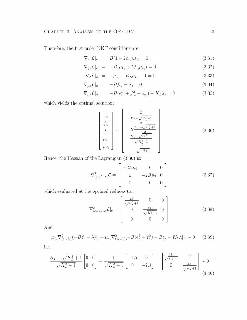
Chapter 3. Analysis of the OPF-DM 53
Therefore, the first order KKT conditions are:
∇erL|c = B(1− 2erc)µ2c = 0 (3.31)
∇frL|c = −B(µ1c + 2frcµ2c) = 0 (3.32)
∇λL|c = −µ1c −KLµ2c − 1 = 0 (3.33)
∇µ1L|c = −Bfrc − λc = 0 (3.34)
∇µ2L|c = −B(e2
rc+ f 2
rc− erc)−KLλc = 0 (3.35)
which yields the optimal solution:
erc
frc
λc
µ1c
µ2c
=
12
KL−√
K2
L+1
2
−BKL−√
K2
L+1
2
KL−√
K2
L+1√K2
L+1
− 1√K2
L+1
(3.36)
Hence, the Hessian of the Lagrangian (3.30) is:
∇2(er ,fr,λ)L =
−2Bµ2 0 0
0 −2Bµ2 0
0 0 0
(3.37)
which evaluated at the optimal reduces to:
∇2(er ,fr,λ)L|c =
2B√K2
L+10 0
0 2B√K2
L+10
0 0 0
(3.38)
And
µ1c∇2(er ,fr)(−Bfr − λ)|c + µ2c∇2
(er ,fr)[−B(e2r + f 2
r ) + Ber −KLλ]|c ≻ 0 (3.39)
i.e.,
KL −√
K2L + 1√
K2L + 1
[0 0
0 0
]− 1√
K2L + 1
[−2B 0
0 −2B
]=
2B√K2
L+10
0 2B√K2
L+1
≻ 0
(3.40)
Chapter 3. Analysis of the OPF-DM 54
Other types of bifurcations for systems with codimension 2 and higher are stud-
ied in [90], which may have similar forms as (3.4), however, these types of bifurca-
tions are out of the scope of this thesis.
The theorem below shows that an optimal solution of (2.20), at which a given
generator is at its reactive power limit while its terminal voltage is at its regulator
set point, corresponds to a LISB and cannot be a LIDB. This is something one can
intuitively deduce from Figure 2.5, if the OS assumptions are met.
Theorem 3.1. Let (zc, λc), zc = (zc, rc), be a local optimum of (2.20) that meets
the aforementioned OS assumptions for p = po, where a given generator i satisfies:
QGic= QGimax
VGic= VGio
}⇒ Vai
= Vbi= 0 (3.41)
while some other generators j 6= i ∈ Gj ⊂ G satisfy:
QGjc= QGjmax
VGjc< VGjo
}⇒
{Vaj
= 0
Vbj> 0
(3.42)
and the rest of the generators 6= j 6= i ∈ G ⊂ G are not at their reactive power
limits, i.e.,
QGmin< QGc
< QGmax
VGc= VGo
}⇒ Va = Vb = 0 (3.43)
(Assumptions (3.42) generalizes the case where a LISB occurs after a LIDB in λ
space, as depicted in Figure 2.5.) Then, (zc, λc, po) is a LISB of the power flow
model defined by equations (2.20b)-(2.20e).
Proof. Let QG = (QG, QGi), i.e., the generator reactive power variables are ordered
so that generator i is the last variable; similarly for VG, Va and Vb. Hence, the
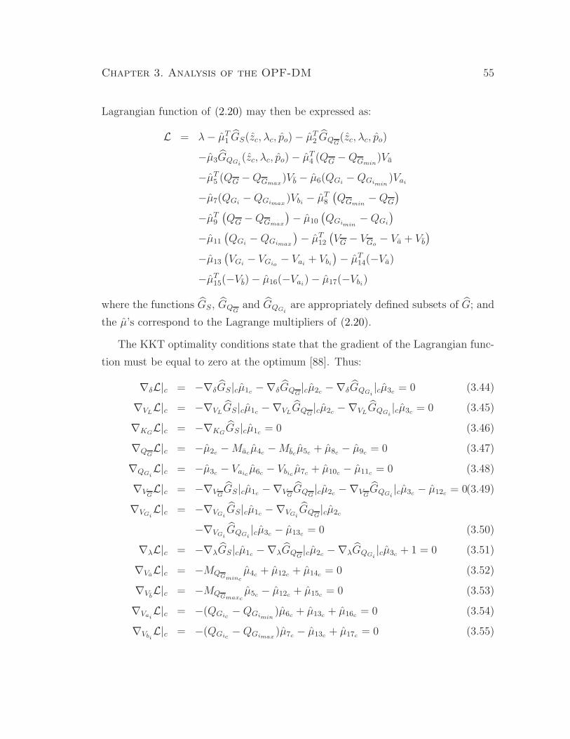
Chapter 3. Analysis of the OPF-DM 55
Lagrangian function of (2.20) may then be expressed as:
L = λ− µT1 GS(zc, λc, po)− µT
2 GQG(zc, λc, po)
−µ3GQGi(zc, λc, po)− µT
4 (QG −QGmin)Va
−µT5 (QG −QGmax
)Vb − µ6(QGi−QGimin
)Vai
−µ7(QGi−QGimax
)Vbi− µT
8
(QGmin
−QG
)
−µT9
(QG −QGmax
)− µ10
(QGimin
−QGi
)
−µ11
(QGi−QGimax
)− µT
12
(VG − VGo
− Va + Vb
)
−µ13
(VGi− VGio
− Vai+ Vbi
)− µT
14(−Va)
−µT15(−Vb)− µ16(−Vai
)− µ17(−Vbi)
where the functions GS, GQGand GQGi
are appropriately defined subsets of G; and
the µ’s correspond to the Lagrange multipliers of (2.20).
The KKT optimality conditions state that the gradient of the Lagrangian func-
tion must be equal to zero at the optimum [88]. Thus:
∇δL|c = −∇δGS|cµ1c −∇δGQG|cµ2c −∇δGQGi
|cµ3c = 0 (3.44)
∇VLL|c = −∇VL
GS|cµ1c −∇VLGQG|cµ2c −∇VL
GQGi|cµ3c = 0 (3.45)
∇KGL|c = −∇KG
GS|cµ1c = 0 (3.46)
∇QGL|c = −µ2c −Mac µ4c −Mbc
µ5c + µ8c − µ9c = 0 (3.47)
∇QGiL|c = −µ3c − Vaic
µ6c − Vbicµ7c + µ10c − µ11c = 0 (3.48)
∇VGL|c = −∇VG
GS|cµ1c −∇VGGQG|cµ2c −∇VG
GQGi|cµ3c − µ12c = 0(3.49)
∇VGiL|c = −∇VGi
GS|cµ1c −∇VGiGQG|cµ2c
−∇VGiGQGi
|cµ3c − µ13c = 0 (3.50)
∇λL|c = −∇λGS|cµ1c −∇λGQG|cµ2c −∇λGQGi
|cµ3c + 1 = 0 (3.51)
∇VaL|c = −MQGmincµ4c + µ12c + µ14c = 0 (3.52)
∇VbL|c = −MQGmaxc
µ5c − µ12c + µ15c = 0 (3.53)
∇VaiL|c = −(QGic
−QGimin)µ6c + µ13c + µ16c = 0 (3.54)
∇VbiL|c = −(QGic
−QGimax)µ7c − µ13c + µ17c = 0 (3.55)
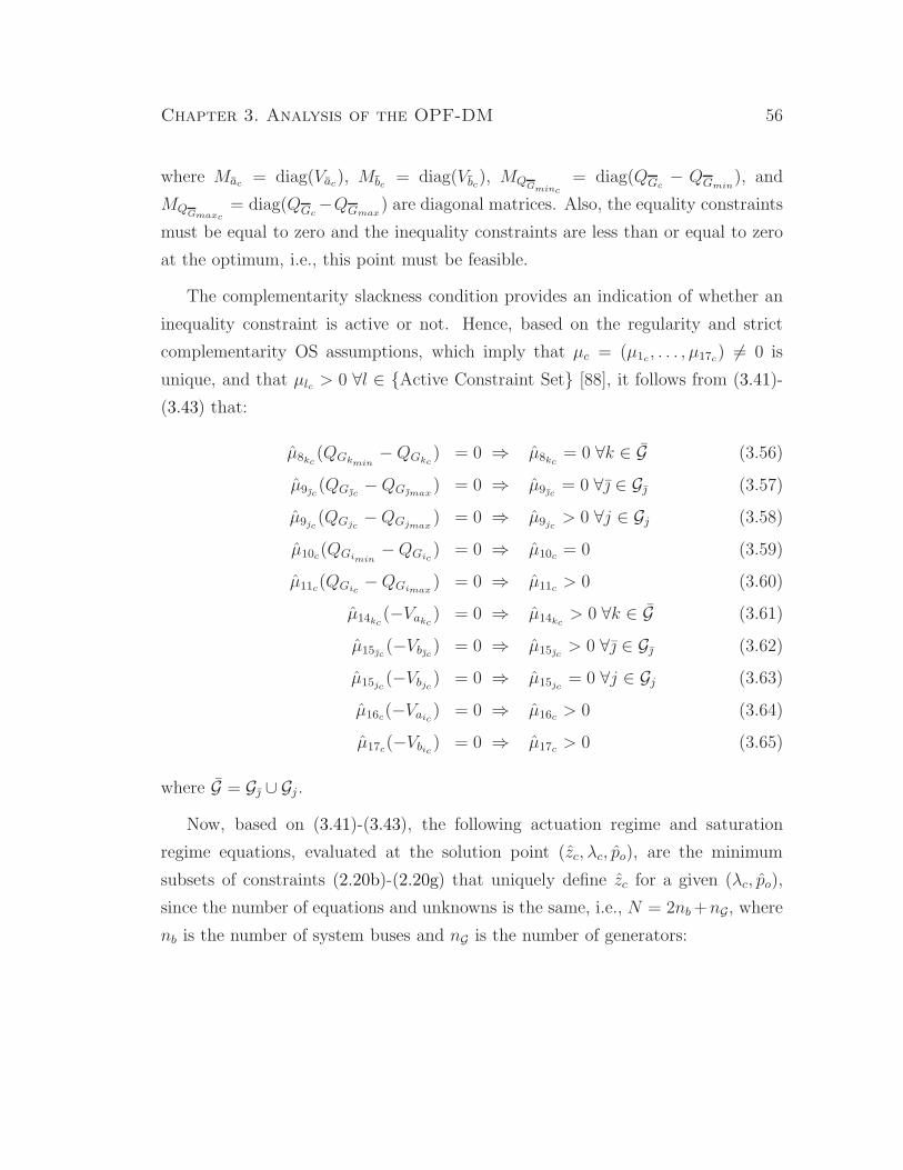
Chapter 3. Analysis of the OPF-DM 56
where Mac = diag(Vac), Mbc= diag(Vbc
), MQGminc= diag(QGc
− QGmin), and
MQGmaxc= diag(QGc
−QGmax) are diagonal matrices. Also, the equality constraints
must be equal to zero and the inequality constraints are less than or equal to zero
at the optimum, i.e., this point must be feasible.
The complementarity slackness condition provides an indication of whether an
inequality constraint is active or not. Hence, based on the regularity and strict
complementarity OS assumptions, which imply that µc = (µ1c , . . . , µ17c) 6= 0 is
unique, and that µlc > 0 ∀l ∈ {Active Constraint Set} [88], it follows from (3.41)-
(3.43) that:
µ8kc(QGkmin
−QGkc) = 0 ⇒ µ8kc
= 0 ∀k ∈ G (3.56)
µ9c(QGc
−QGmax) = 0 ⇒ µ9c
= 0 ∀ ∈ G (3.57)
µ9jc(QGjc
−QGjmax) = 0 ⇒ µ9jc
> 0 ∀j ∈ Gj (3.58)
µ10c(QGimin−QGic
) = 0 ⇒ µ10c = 0 (3.59)
µ11c(QGic−QGimax
) = 0 ⇒ µ11c > 0 (3.60)
µ14kc(−Vakc
) = 0 ⇒ µ14kc> 0 ∀k ∈ G (3.61)
µ15c(−Vbc
) = 0 ⇒ µ15c> 0 ∀ ∈ G (3.62)
µ15jc(−Vbjc
) = 0 ⇒ µ15jc= 0 ∀j ∈ Gj (3.63)
µ16c(−Vaic) = 0 ⇒ µ16c > 0 (3.64)
µ17c(−Vbic) = 0 ⇒ µ17c > 0 (3.65)
where G = G ∪ Gj .
Now, based on (3.41)-(3.43), the following actuation regime and saturation
regime equations, evaluated at the solution point (zc, λc, po), are the minimum
subsets of constraints (2.20b)-(2.20g) that uniquely define zc for a given (λc, po),
since the number of equations and unknowns is the same, i.e., N = 2nb +nG, where
nb is the number of system buses and nG is the number of generators:

Chapter 3. Analysis of the OPF-DM 57
Ga|c =
G(δc, VLc , KGc, QGc , VGc, λc, PSo, PDo)
VGc− VGo
∀ ∈ G
QGjc−QGjmax
∀j ∈ Gj
VGic− VGio
= 0 (3.66)
Gb|c =
G(δc, VLc , KGc , QGc , VGc , λc, PSo, PDo)
VGc− VGo
∀ ∈ G
QGjc−QGjmax
∀j ∈ Gj
QGic−QGimax
= 0 (3.67)
Notice that these equations have a similar form as (2.8) and (2.9) respectively,
where zc = (δc, VLc , KGc, VGc), rc = QGc , po = (PSo , PDo, VGo), g|c = G|c, and
rc–s|c ≡
VGc− VGo
∀ ∈ G
QGjc−QGjmax
∀j ∈ Gj
VGic− VGio
(3.68)
Observe that in this case, some of the actuation limit functions are implicit
instead of explicit functions of the corresponding variables r. Hence, for the optimal
solution to be a LISB, one must first prove that the Jacobians J ia and J i
b associated
with (3.66) and (3.67) are nonsingular.
Let first prove that J ib is not singular. Hence, from (3.44)-(3.55) and with
the proper ordering of variables and equations in (3.67), and assuming that VG =
(VG ∀ ∈ G, VGj∀j ∈ Gj), and similarly for QG, it can be shown that:
J iT
b xb = bb (3.69)
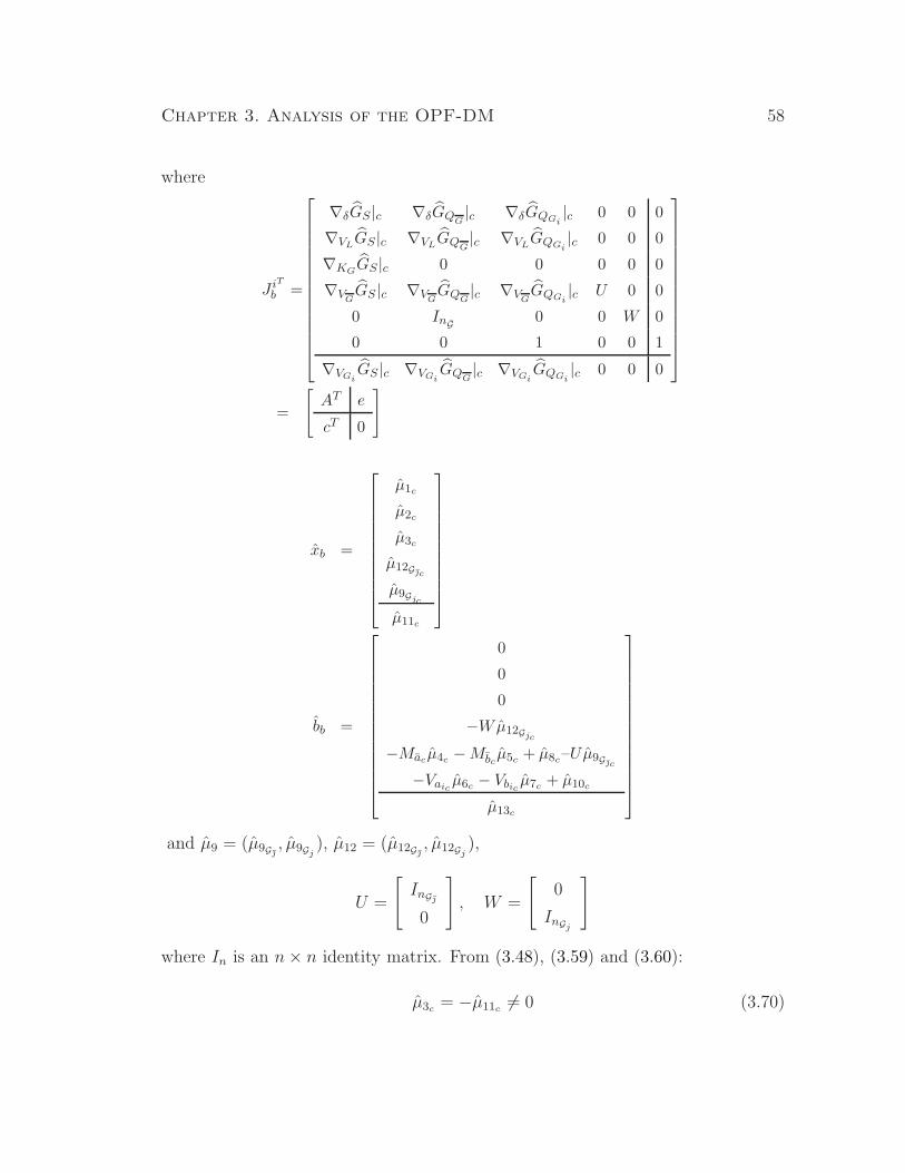
Chapter 3. Analysis of the OPF-DM 58
where
J iT
b =
∇δGS |c ∇δGQG|c ∇δGQGi
|c 0 0 0
∇VLGS |c ∇VL
GQG|c ∇VL
GQGi|c 0 0 0
∇KGGS |c 0 0 0 0 0
∇VGGS |c ∇VG
GQG|c ∇VG
GQGi|c U 0 0
0 InG0 0 W 0
0 0 1 0 0 1
∇VGiGS |c ∇VGi
GQG|c ∇VGi
GQGi|c 0 0 0
=
[AT e
cT 0
]
xb =
µ1c
µ2c
µ3c
µ12Gc
µ9Gjc
µ11c
bb =
0
0
0
−Wµ12Gjc
−Macµ4c −Mbcµ5c + µ8c–Uµ9Gc
−Vaicµ6c − Vbic
µ7c + µ10c
µ13c
and µ9 = (µ9G, µ9Gj
), µ12 = (µ12G, µ12Gj
),
U =
[InG
0
], W =
[0
InGj
]
where In is an n× n identity matrix. From (3.48), (3.59) and (3.60):
µ3c = −µ11c 6= 0 (3.70)
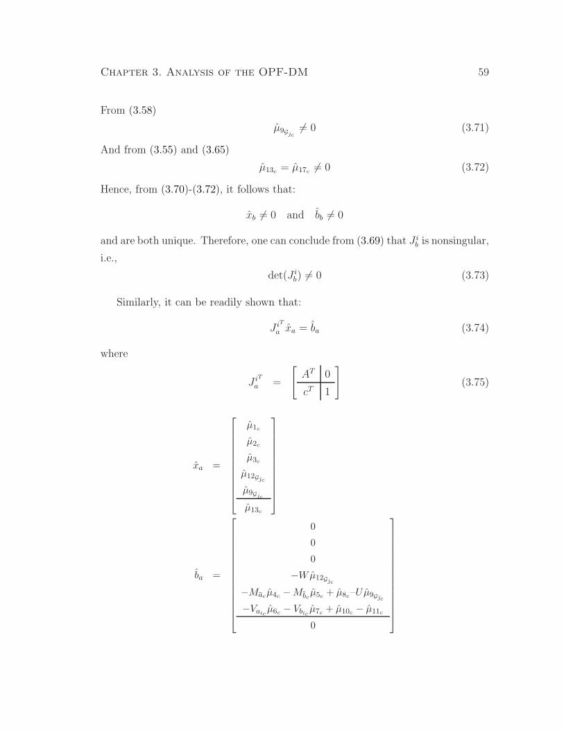
Chapter 3. Analysis of the OPF-DM 59
From (3.58)
µ9Gjc6= 0 (3.71)
And from (3.55) and (3.65)
µ13c = µ17c 6= 0 (3.72)
Hence, from (3.70)-(3.72), it follows that:
xb 6= 0 and bb 6= 0
and are both unique. Therefore, one can conclude from (3.69) that J ib is nonsingular,
i.e.,
det(J ib) 6= 0 (3.73)
Similarly, it can be readily shown that:
J iT
a xa = ba (3.74)
where
J iT
a =
[AT 0
cT 1
](3.75)
xa =
µ1c
µ2c
µ3c
µ12Gc
µ9Gjc
µ13c
ba =
0
0
0
−Wµ12Gjc
−Mac µ4c −Mbcµ5c + µ8c–Uµ9Gc
−Vaicµ6c − Vbic
µ7c + µ10c − µ11c
0

Chapter 3. Analysis of the OPF-DM 60
Therefore, from (3.70)-(3.72), it follows that:
xa 6= 0 and ba 6= 0
and are both unique, yielding a nonsingular J ia, from (3.74) i.e.,
det(J ia) 6= 0 (3.76)
Thus, from (3.73) and (3.76), it is clear that the solution point (zc, λc, po) meets
transversality conditions (2.10).
The second transversality condition (2.11) simply states that the ratio of the
determinants of J ia and J i
b must be positive for (zc, λc, po) to be a LISB. Thus, from
(3.70) and (3.75), and based on Schur’s Complements [91], it follows that:
det(J ia) = det(A)
det(J ib) = −eT A−1c det(A)
Therefore:
α =det(J i
a)
det(J ib)
=1
−eT A−1c(3.77)
Now, from (3.66), it follows that:
∇Tz Ga|c dz +∇T
VGioGa|c dVGio
= 0
which from (3.75) can be rewritten as:[
A c
0 1
][dz
dVGi
]−[
0
1
]dVGio
= 0
where z = (z, VGi). This yields:
dz = −A−1c dVGi(3.78)
dVGi= dVGio
(3.79)
On the other hand, from (3.67) and (3.70), one knows that:[
A c
eT 0
][dz
dVGi
]−[
0
1
]dQGimax
= 0
Chapter 3. Analysis of the OPF-DM 61
which yields (3.78) as well as:
dQGi= eT dz = dQGimax
(3.80)
Thus, from (3.78), (3.79) and (3.80), it follows that:
dQGimax
dVGio
∣∣∣∣c
= −eT A−1c
which, from (3.77), leads to:
α =dVGio
dQGimax
∣∣∣∣c
(3.81)
Now, from the optimization model (2.20), the sensitivities of the objective func-
tion with respect to QGimaxand VGio
evaluated at the optimal point can be stated
as [92]:
µ11c =dλ
dQGimax
∣∣∣∣c
µ13c =dλ
dVGio
∣∣∣∣c
Hence, from (3.60), (3.72), and (3.81), it follows that:
α =µ11c
µ13c
> 0 (3.82)
which satisfies the second transversality condition (2.11). Therefore, the optimal
solution (zc, λc, po) which meets the given OS assumptions is a LISB.
Finally, observe that at a LIDB, assumptions (3.41)-(3.43) are also met. How-
ever, (3.82) rules out the possibility of a LIDB being a solution of (2.20).
This theorem basically proves that a given local optimum of (2.20) can be a
LISB and not a LIDB, and that it can be preceded by some generators reaching
reactive power limits, i.e., LIDBs. The following theorem shows that this local
optimum can also be an SNB.
Chapter 3. Analysis of the OPF-DM 62
Theorem 3.2. Let (zc, λc) be local optimum of (2.20) that meets the abovemen-
tioned OS assumptions for p = po, where some generators j ∈ Gj ⊂ G satisfy:
QGjc= QGjmax
VGjc< VGjo
}⇒
{Vaj
= 0
Vbj> 0
(3.83)
while the rest of the generators 6= j ∈ G ⊂ G, G = G∪Gj, are not at their reactive
power limits, i.e.,
QGmin< QGc
< QGmax
VGc= VGo
}⇒ Va = Vb = 0 (3.84)
(Assumptions (3.83) and (3.84) generalize the case where an SNB occurs after a
LIDB in λ space, as depicted in Figure 2.3.) Then, (zc, λc, po) is an SNB of the
power flow model defined by equations (2.20b)-(2.20e).
Proof. Following a similar approach to the proof of Theorem 3.1, let QG = (QG, QG),
where QG = (QG ∀ ∈ G, QGj∀j ∈ Gj), and similarly for VG, Va and Vb. Hence,
the Lagrangian function of (2.20) may then be expressed as:
L = λ− µT1 GS(zc, λc, po)− µT
2 GQG(zc, λc, po)
−µ3GQG(zc, λc, po)− µT
4 (QG −QGmin)Va
−µT5 (QG −QGmax
)Vb − µT6 (Q
G−Q
Gmin)Va
−µT7 (QG −QGmax
)Vb − µT8
(QGmin
−QG
)
−µT9
(QG −QGmax
)− µT
10
(Q
Gmin−Q
G
)
−µT11
(QG −QGmax
)− µT
12
(VG − VGo
− Va + Vb
)
−µ13
(VG − VGo
− Va + Vb
)− µT
14(−Va)
−µT15(−Vb)− µT
16(−Va)− µT17(−Vb)

Chapter 3. Analysis of the OPF-DM 63
From the KKT optimality conditions, it follows that:
∇δL|c = −∇δGS |cµ1c −∇δGQG|cµ2c −∇δGQ
G|cµ3c = 0 (3.85)
∇VLL|c = −∇VL
GS |cµ1c −∇VLGQG
|cµ2c −∇VLGQ
G|cµ3c = 0 (3.86)
∇KGL|c = −∇KG
GS |cµ1c = 0 (3.87)
∇QGL|c = −µ2c −Mac µ4c −Mbc
µ5c + µ8c − µ9c = 0 (3.88)
∇QGL|c = −µ3c −Mac µ6c −M
bcµ7c + µ10c − µ11c = 0 (3.89)
∇VGL|c = −∇VG
GS |cµ1c −∇VGGQG
|cµ2c −∇VGGQ
G|cµ3c − µ12c = 0 (3.90)
∇VGL|c = −∇V
GGS |cµ1c −∇V
GGQG
|cµ2c −∇VGGQ
G|cµ3c − µ13c = 0 (3.91)
∇λL|c = −∇λGS |cµ1c −∇λGQG|cµ2c −∇λGQ
G|cµ3c + 1 = 0 (3.92)
∇VaL|c = −MQGmincµ4c + µ12c + µ14c = 0 (3.93)
∇VbL|c = −MQGmaxc
µ5c − µ12c + µ15c = 0 (3.94)
∇VaL|c = −MQ
Gminc
µ6c + µ13c + µ16c = 0 (3.95)
∇VbL|c = −MQ
Gmaxcµ7c − µ13c + µ17c = 0 (3.96)
where Mac = diag(Vac), and similarly for Mbc, Mac , Mbc
; and MQGminc= diag(QGc
−QGmin
), and similarly for MQGmaxc, MQ
Gminc
, and MQGmaxc
. Furthermore, all the
equality constraints must be equal to zero, while the inequality constraints must
be less than or equal to zero.
From the regularity and strict complementarity OS assumptions, which imply
a unique µc = (µ1c , . . . , µ17c) 6= 0, with µlc > 0 ∀l ∈ {Active Constraint Set}, it
follows from (3.83) and (3.84) that:
µ8c(QGmin
−QGc) = 0 ⇒ µ8c
= 0 ∀ ∈ G (3.97)
µ9c(QGc
−QGmax) = 0 ⇒ µ9c
= 0 ∀ ∈ G (3.98)
µ10jc(QGjmin
−QGjc) = 0 ⇒ µ10jc
= 0 ∀j ∈ Gj (3.99)
µ11jc(QGjc
−QGjmax) = 0 ⇒ µ11jc
> 0 ∀j ∈ Gj (3.100)
µ14c(−Vac
) = 0 ⇒ µ14c> 0 ∀ ∈ G (3.101)
µ15c(−Vbc
) = 0 ⇒ µ15c> 0 ∀ ∈ G (3.102)
µ16jc(−Vajc
) = 0 ⇒ µ16jc> 0 ∀j ∈ Gj (3.103)
Chapter 3. Analysis of the OPF-DM 64
µ17jc(−Vbjc
) = 0 ⇒ µ17jc= 0 ∀j ∈ Gj (3.104)
Now, based on (3.83) and (3.84), the following equations, evaluated at the solu-
tion point (zc, λc, po), form the minimum subset of constraints (2.20b)-(2.20g) that
uniquely define zc for a given (λc, po), since the number of equations and unknowns
are the same, i.e., N :
G|c =
G(δc, VLc , KGc , QGc , VGc, λc, PSo, PDo)
VGc− VGo
QGc−Q
Gmax
= 0 (3.105)
Hence, for the optimal solution to be an SNB, one must first prove that the
Jacobian J = ∇Tz G|c is singular with unique nonzero eigenvectors, where z =
(δ, VL, KG, VG, QG).
From (3.85)-(3.96) and with the proper ordering of variables and equations in
(3.67), it can be shown that:
∇zG|c w = b (3.106)
where,
∇zG|c =
∇δGS|c ∇δGQG|c ∇δGQ
G|c 0 0
∇VLGS|c ∇VL
GQG|c ∇VL
GQG|c 0 0
∇KGGS|c 0 0 0 0
∇VGGS|c ∇VG
GQG|c ∇VG
GQG|c InG
0
∇VGGS|c ∇V
GGQG|c ∇V
GGQ
G|c 0 0
0 InG0 0 0
0 0 InGj0 InGj
(3.107)
Chapter 3. Analysis of the OPF-DM 65
w =
µ1c
µ2c
µ3c
µ12c
µ11c + Mbcµ7c
(3.108)
b =
0
0
0
0
−µ13c
−Mac µ4c −Mbcµ5c + µ8c–µ9c
−Mac µ6c + µ10c
Now, from (3.96) and (3.104):
µ13c = µ17c = 0 (3.109)
From (3.84), (3.97) and (3.98):
−Mac µ4c −Mbcµ5c + µ8c–µ9c = 0 (3.110)
From (3.83) and (3.99):
−Mac µ6c + µ10c = 0 (3.111)
Hence, from (3.109)-(3.111), it follows that:
∇zG|c w = 0
Finally, from the regularity and strict complementarity OS assumptions, it follows
that µ1c 6= 0, µ2c 6= 0, and µ3c 6= 0, as µc 6= 0 and is unique. Hence, w 6= 0 and
is unique, from which it can be concluded that the optimum (zc, λc, po) meets the
SNB transversality condition (2.3).
Chapter 3. Analysis of the OPF-DM 66
Now, from (3.92), (3.105) and (3.108), it follows that:
∇λL|c = −∇λG|c w + 1 = 0
⇒ ∇λG|c w 6= 0
which corresponds to the SNB transversality condition (2.4).
The third SNB transversality condition (2.5) is now verified. Thus, from as-
sumptions (3.83) and (3.84) regarding the optimum (zc, λc, po), and from (3.105),
as well as based on the previous analysis, the optimization model (2.20) can be
restated as follows, since it would yield the same optimal solution:
max λ
s.t. G(z, λ, po) = 0
The corresponding Lagrangian function may then be defined as:
L(z, λ, po, µ) = λ− µT G(z, λ, po)
which, based on the KKT optimality conditions, leads to:
∇zL|c = −∇zG|cµc = −∇zG|cw = 0 (3.113)
∇µL|c = −G|c = 0 (3.114)
∇λL|c = −∇λG|cw + 1 = 0 (3.115)
Based on the OS assumptions, which guarantee that the set of equations (3.113)-
(3.115) have a unique solution, the full Hessian of the Lagrangian function, i.e., the
Jacobian of these equations, must be nonsingular; thus:
∇2(z,µ,λ)L(zc, λc, po, w) ρ 6= 0 ∀ρ 6= 0 (3.116)
where
∇2(z,µ,λ)L|c = −
∇2zG|cw ∇zG|c ∇2
λzG|cw∇T
z G|c 0 ∇TλG|c
wT∇2T
zλG|c ∇λG|c ∇2λG|cw
(3.117)

Chapter 3. Analysis of the OPF-DM 67
Hence, for a chosen ρ = (v, 0, 0) 6= 0, from (3.116) one has that:
[∇2
zG|cw]v 6= 0 (3.118)
since, in this case, ∇2T
zλG|c = ∇2λzG|c = 0. On the other hand, from the second-order
KKT necessary optimality conditions [88]:
ρT ∇2(z,λ)L|c ρ ≤ 0 ∀ρ ∈ U(zc, λc) (3.119)
where
U(zc, λc) ={ρ ∈ R
nz+1 :[∇T
z G|c∇TλG|c
]ρ = 0
}
Hence, for ρ = (v, 0) it follows from (3.117) and (3.119) that:
vT[∇2
zG|cw]v ≥ 0
Therefore, from (3.118), it can be concluded that:
vT[∇2
zG|cw]v > 0
Finally, taking the transpose of this equation and considering the properties of
tensor products:
wT[∇2T
z G|cv]v > 0
This corresponds to the third SNB transversality condition (2.5).
It is important to highlight that this theorem proves that the solution is not
simply a fold but an SNB, since the uniqueness of the zero eigenvectors is demon-
strated here. Finally, the following corollary argues that an optimum of (2.20) can
only be a LISB or an SNB.
Corollary 3.1. Any solution point (zc, λc, po) of (2.20) that meets the aforemen-
tioned OS assumptions is either a LISB or an SNB.
Proof. Observe that Theorem 3.1 proofs that a LIDB cannot be a solution of (2.20).
Now, notice that all possible limit conditions of the inequality constraints of (2.20)
Chapter 3. Analysis of the OPF-DM 68
are considered in assumptions (3.41)-(3.43) and (3.83)-(3.84) of Theorems 3.1 and
3.2, respectively. Thus, the cases of none or all generators reaching their limits
are simply particular cases of these assumptions. Hence, any feasible solution of
(2.20), would either meet assumptions (3.41)-(3.43) or (3.83)-(3.84). Therefore, the
solution point (zc, λc, po) can only be a LISB or a SNB.
3.3 Numerical Examples
This section presents a numerical comparison between the OPF-DM and the CPF
method to illustrate some of the theoretical issues discussed in the previous section.
Thus, the maximum loading factor, voltage, and reactive power levels obtained
from solving (2.20) are compared with those obtained using the standard CPF,
for a variety of test cases for the 6-bus system shown in Figure A.1 [1]. In these
cases, the generators’ voltage set points and reactive power limits are assumed to
be VGo = 1.05 p.u. and QG = ±1.5 p.u., respectively. The CIGRE-32 test system
described in Appendix A is also used to compare both techniques.
3.3.1 Practical Implementation Issues
The OPF-DM with complementarity constraints can be implemented in AMPL,
using the complements operator [93, 94], which allows complementarity conditions
to be directly specified in the constraint declarations, and then solved using solvers
specifically designed for complementarity problems such as KNITRO [95]. Alterna-
tively, the complementarity constraints can be specified as nonsmooth constraints
as in (2.20), solving the optimization problem with nonlinear programming solvers
such as LOQO, KNITRO or IPOPT. This second approach is used here to obtain
the numerical results discussed in this section. On the other hand, UWPFLOW [72],
which is a popular and well-tested software tool with a robust implementation of
a CPF technique, was used to obtain PV curves for illustrative and comparison
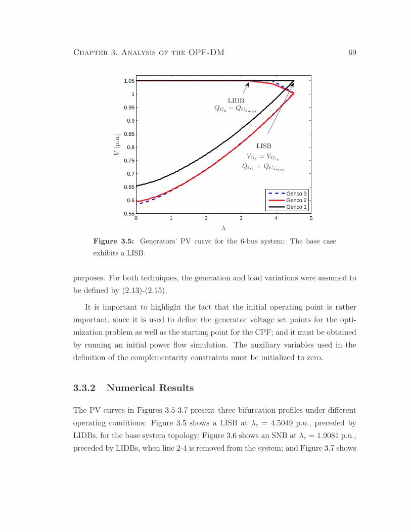
Chapter 3. Analysis of the OPF-DM 69
0 1 2 3 4 50.55
0.6
0.65
0.7
0.75
0.8
0.85
0.9
0.95
1
1.05
Genco 3Genco 2Genco 1
λ
V[p
.u.]
VG1= VG1o
QG1= QG1max
LISB
LIDBQG2
= QG2max
Figure 3.5: Generators’ PV curve for the 6-bus system: The base case
exhibits a LISB.
purposes. For both techniques, the generation and load variations were assumed to
be defined by (2.13)-(2.15).
It is important to highlight the fact that the initial operating point is rather
important, since it is used to define the generator voltage set points for the opti-
mization problem as well as the starting point for the CPF; and it must be obtained
by running an initial power flow simulation. The auxiliary variables used in the
definition of the complementarity constraints must be initialized to zero.
3.3.2 Numerical Results
The PV curves in Figures 3.5-3.7 present three bifurcation profiles under different
operating conditions: Figure 3.5 shows a LISB at λc = 4.5049 p.u., preceded by
LIDBs, for the base system topology; Figure 3.6 shows an SNB at λc = 1.9081 p.u.,
preceded by LIDBs, when line 2-4 is removed from the system; and Figure 3.7 shows
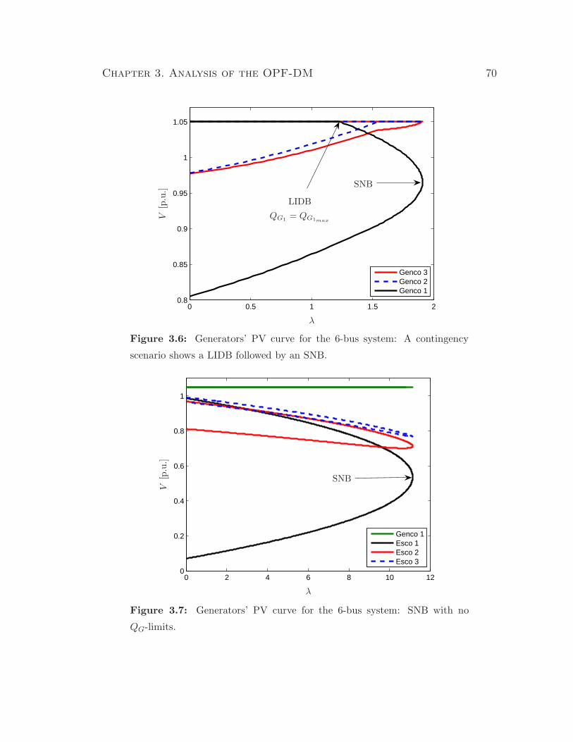
Chapter 3. Analysis of the OPF-DM 70
0 0.5 1 1.5 20.8
0.85
0.9
0.95
1
1.05
Genco 3Genco 2Genco 1
λ
V[p
.u.]
LIDB
QG1= QG1max
SNB
Figure 3.6: Generators’ PV curve for the 6-bus system: A contingency
scenario shows a LIDB followed by an SNB.
0 2 4 6 8 10 120
0.2
0.4
0.6
0.8
1
Genco 1Esco 1Esco 2Esco 3
λ
V[p
.u.]
SNB
Figure 3.7: Generators’ PV curve for the 6-bus system: SNB with no
QG-limits.
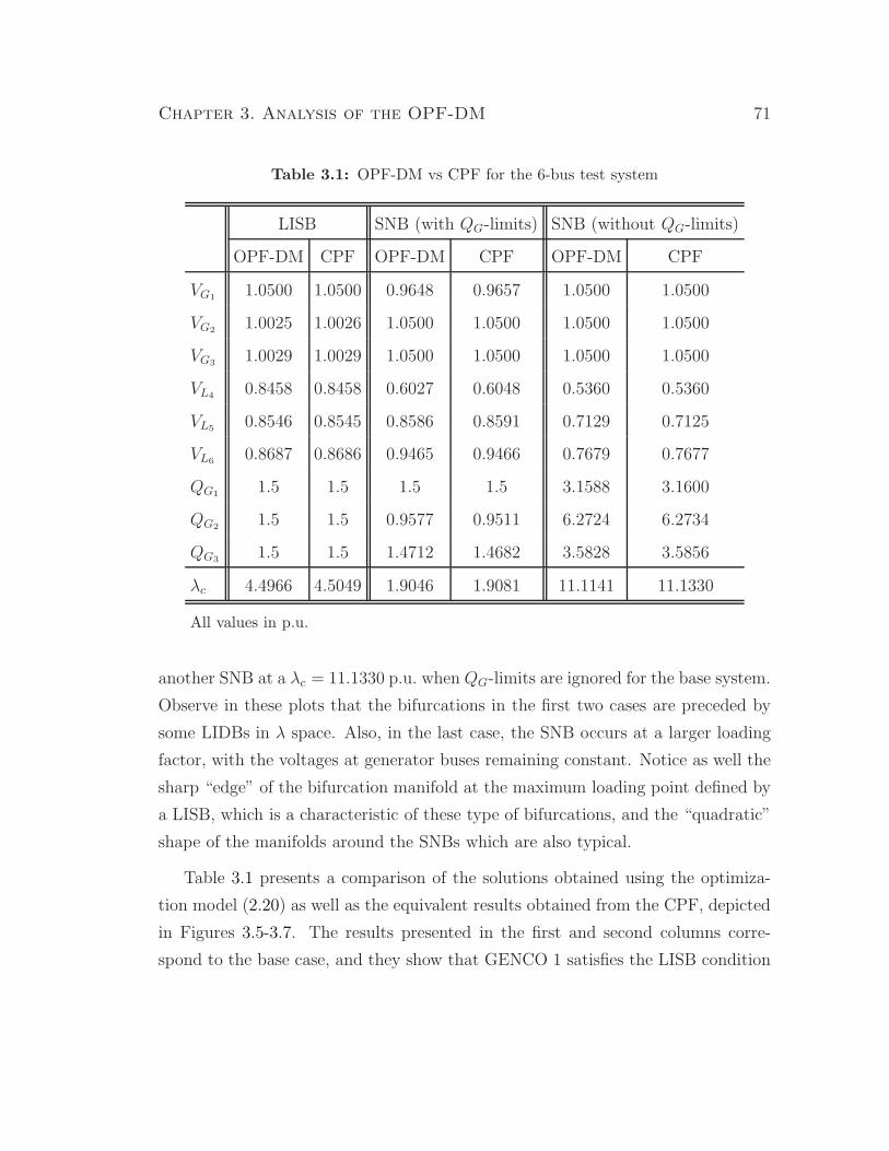
Chapter 3. Analysis of the OPF-DM 71
Table 3.1: OPF-DM vs CPF for the 6-bus test system
LISB SNB (with QG-limits) SNB (without QG-limits)
OPF-DM CPF OPF-DM CPF OPF-DM CPF
VG11.0500 1.0500 0.9648 0.9657 1.0500 1.0500
VG21.0025 1.0026 1.0500 1.0500 1.0500 1.0500
VG31.0029 1.0029 1.0500 1.0500 1.0500 1.0500
VL40.8458 0.8458 0.6027 0.6048 0.5360 0.5360
VL50.8546 0.8545 0.8586 0.8591 0.7129 0.7125
VL60.8687 0.8686 0.9465 0.9466 0.7679 0.7677
QG11.5 1.5 1.5 1.5 3.1588 3.1600
QG21.5 1.5 0.9577 0.9511 6.2724 6.2734
QG31.5 1.5 1.4712 1.4682 3.5828 3.5856
λc 4.4966 4.5049 1.9046 1.9081 11.1141 11.1330
All values in p.u.
another SNB at a λc = 11.1330 p.u. when QG-limits are ignored for the base system.
Observe in these plots that the bifurcations in the first two cases are preceded by
some LIDBs in λ space. Also, in the last case, the SNB occurs at a larger loading
factor, with the voltages at generator buses remaining constant. Notice as well the
sharp “edge” of the bifurcation manifold at the maximum loading point defined by
a LISB, which is a characteristic of these type of bifurcations, and the “quadratic”
shape of the manifolds around the SNBs which are also typical.
Table 3.1 presents a comparison of the solutions obtained using the optimiza-
tion model (2.20) as well as the equivalent results obtained from the CPF, depicted
in Figures 3.5-3.7. The results presented in the first and second columns corre-
spond to the base case, and they show that GENCO 1 satisfies the LISB condition
Chapter 3. Analysis of the OPF-DM 72
QG1c= QG1max
and VG1c= VG1o
at λc, while GENCO 2 and GENCO 3 are at their
reactive power limits with their voltages below the corresponding set points. That
is, the system has undergone 2 LIDBs before reaching a LISB in λ space, as clearly
illustrated in Figure 3.5. The results in the third and fourth columns, obtained by
removing line 2-4, show GENCO 2 and GENCO 3 within their reactive power limits
and at their corresponding voltage set points. Meanwhile, GENCO 1 has reached
its maximum reactive power limit and its voltage is below its set point, indicating
the occurrence of a LIDB before the SNB in λ space, as depicted in Figure 3.6.
Finally, the results presented in the last two columns, which correspond to the base
system without generator reactive power limits, show all generators at their volt-
age set points as well as large reactive power outputs. That is, there are no LIDBs
before the SNB in λ space. This table shows that both techniques essentially give
the same solution; the small differences can be basically attributed to numerical
approximations, particularly in the case of the CPF. The execution time for the
OPF-DM was in the range of 0.12s, which was faster than the CPF.
The sequence of generators reaching the maximum reactive power limit can be
also obtained from the OPF-DM, by ranking the difference ∆VGic= VGio
− VGicin
descending order. Thus, the largest difference corresponds to the first generator’s
reaching its maximum reactive power limit, and so on. If the difference is negative,
then the generator would have reached the minimum reactive power limit. For
example, the ranked differences for the base case are: ∆VG2c= 0.0475, ∆VG3c
=
0.0471 and ∆VG1c= 0, which agrees with what is observed in Figure 3.5.
A test was carried out to study the effect of setting the upper voltage limits
at generation buses at their corresponding set points for the model without com-
plementarity constraints (2.17), with the objective that by defining VGmax = VGo ,
the optimization solution process would “fix” the generator voltages at their ini-
tial maximum voltage levels. This would yield similar results as those obtained by
solving (2.20), since voltages at generation buses, if not fixed, typically increase
when increasing the load. It is interesting to notice that this approach generated
the same results as those depicted in Table 3.1. However, this was not the case for

Chapter 3. Analysis of the OPF-DM 73
0 0.05 0.1 0.15
0.86
0.88
0.9
0.92
0.94
0.96
0.98
4042424043
λ
V[p
.u.]
Figure 3.8: PV curve for the CIGRE-32 test system: The base case exhibits
an SNB.
0 0.1 0.2 0.3 0.4 0.5 0.6 0.7 0.80.65
0.7
0.75
0.8
0.85
0.9
0.95 232439
λ
V[p
.u.]
Figure 3.9: PV curve for the CIGRE-32 system: SNB with no QG-limits.

Chapter 3. Analysis of the OPF-DM 74
other test systems, since (2.17) does not necessarily guarantee that generators are
going to be at their maximum voltage values (voltage set points in this case) if their
reactive power limits have not been reached. For instance, Table 3.2 summarizes
the results for the CIGRE-32 test system corresponding to the PV curves shown
in Figure 3.8 and Figure 3.9, where an SNB at λ = 0.1473, and at λ = 0.8144
are shown for the base case and neglecting QG-limits, respectively. Observe in this
table that the reactive power at some buses is significantly different from that ob-
tained using CPF, if complementarity constraints are not used. Also notice that in
some generators:
• VG = VGo when the reactive power is within limits, e.g., QG4047max= 6.0 p.u.,
and VGo4044= 0.9473 p.u.
• VG < VGo if a QG-limit is reached, e.g., QG4042max= 3.5 p.u., and VGo4042
=
0.9831 p.u.
• both QG and VG are set to the upper limit, e.g., QG4011max= 5.0 p.u.,
QG4012max= 4.0 p.u., VGo4011
= 1.05 p.u., and VGo4012= 1.04 p.u.
Table 3.2: Comparison of the OPF-DM vs CPF for the CIGRE-32 system
SNB (with QG-limits) SNB (without QG-limits)
OPF-DM CPF OPF-DM CPF
(2.17) (2.20) (2.17) (2.20)
VG40111.0500 1.0500 1.0500 0.9341 1.0500 1.0500
VG40121.0400 1.0400 1.0400 0.2430 1.0400 1.0400
VG40420.9537 0.9521 0.9521 0.9831 0.9831 0.9830
VG420.9314 0.9298 0.9298 0.9457 0.9467 0.9465
VG40430.9075 0.9066 0.9065 0.8099 0.8030 0.8029
VG430.8820 0.8811 0.8810 0.7537 0.7477 0.7476
VG40470.9473 0.9473 0.9470 0.9473 0.9473 0.9470
Continued on next page

Chapter 3. Analysis of the OPF-DM 75
Table 3.2 – continued from previous page
SNB (with QG-limits) SNB (without QG-limits)
OPF-DM CPF OPF-DM CPF
(2.17) (2.20) (2.17) (2.20)
VG40460.9064 0.9059 0.9057 0.8082 0.8064 0.8062
VG470.9235 0.9235 0.9232 0.9067 0.9078 0.9074
VG460.8764 0.8759 0.8757 0.7403 0.7405 0.7402
QG4072-0.2130 4.9683 4.9665 8.7258 8.9849 8.9826
QG40712.5000 1.1419 1.1415 22.1923 2.2520 2.2519
QG40115.0000 0.8662 0.8540 100 9.4523 9.4458
QG40124.0000 -0.6065 -0.6119 -40.4752 1.5048 1.5037
QG40211.5000 1.5000 1.5000 14.0337 11.1244 11.1261
QG40311.7500 1.7500 1.7500 49.0580 23.4120 23.3409
QG40423.5000 3.5000 3.5000 30.1225 34.3495 34.3127
QG40412.0941 2.2167 2.1972 12.3894 15.2220 15.2365
QG40621.7610 1.7601 1.7197 36.9707 10.5022 10.4566
QG40632.2965 2.2905 2.3130 3.4694 5.2850 5.3054
QG40513.5000 3.5000 3.5000 15.9721 16.5290 16.5068
QG40473.7669 3.8447 3.8065 15.2604 15.5880 15.5650
QG20321.3713 1.3802 1.3758 26.2726 4.3197 4.3239
QG10132.2579 1.2057 1.2052 12.1313 2.8660 2.8643
QG1012-0.7905 -0.3673 -0.3678 100 1.9076 1.9058
QG1014-0.9999 0.4218 0.4218 0.6924 0.6075 0.6091
QG10221.2500 1.2500 1.2500 31.5172 12.1901 12.1866
QG10212.7510 2.7467 2.7436 11.6739 6.8142 6.8071
QG10431.0000 1.0000 1.0000 20.0257 20.1360 20.0896
QG10420.4923 0.5040 0.4993 2.7057 2.7233 2.7192
λc 0.1492 0.1476 0.1473 0.8578 0.8148 0.8144
Chapter 3. Analysis of the OPF-DM 76
3.4 Summary
This chapter has presented a detailed, theoretical study of an optimization method
able to determine two types of fold bifurcations directly associated with voltage
instabilities in power systems. It was demonstrated that the necessary and sufficient
optimality conditions yield the transversality conditions for SNBs and LISBs. Thus,
it has been shown that the solution of the studied optimization problem yields the
same results as those obtained with the more popular CPF techniques, which is
typically used to analyze these types of bifurcations in power systems.
The advantages of stating the SNB/LIB problem as an optimization problem
is that optimization solution techniques can be computationally more effective
than CPF methods for maximum loadability studies, particularly when using well-
tested and efficient solution techniques such as IPM. Furthermore, optimization
approaches are more versatile than CPF techniques, since the problem can be read-
ily restated so that optimal control parameter values can be calculated to increase
the maximum loadability margins of a system, or readily carry out a variety of
sensitivity studies.
Chapter 4
Practical Solution of
Voltage-Stability-Constrained
Optimal Power Flows
4.1 Introduction
Chapter 3 demonstrated the feasibility of an optimization method to determine
the voltage collapse point of a power flow model, namely an SNB or LIB point.
This chapter proposes a novel and practical method to enforce a VS constraint in
an OPF auction model, based on the MSV and minimum singular vectors of the
power flow Jacobian. By ensuring that this singular value is bounded from reaching
zero and guaranteeing that generators’ reactive power and other security limits are
met, adequate security margins in a power system can be ensured, hence preventing
a voltage collapse point. The proposed technique is based on a SVD of the power
flow Jacobian at a given solution point, plus an iterative process to satisfy the
VS constraint. A small but realistic, 6-bus test system and a 1211-bus model of
a European grid are used to analyze the performance of the proposed technique.
Comparisons with previously proposed solution techniques for similar VSC-OPFs
77

Chapter 4. Practical Solution of VSC-OPF 78
are presented. The results obtained demonstrate the feasibility of applying the
proposed VSC-OPF in practice.
4.2 Proposed Solution Method
The main objective in the development of the proposed solution method is to re-
place (2.24c) with an equivalent constraint that can be written explicitly in terms
of the VSC-OPF optimization variables. Thus, SVD concepts and an iterative tech-
nique to deal with this constraint in practice are used in the proposed VSC-OPF
method, as described below.
4.2.1 Singular Value Decomposition (SVD)
The SVD is typically used to determine the rank of a matrix, i.e., the maximum
number of independent rows or columns, and it can be used as a measure of how
close a matrix is to the set of singular matrices [96]. Therefore, if the Jacobian
J ∈ Rn×n, where n = 2nb (nb is the number of buses in (2.21b)), is invertible or
nonsingular, this matrix is full rank and its orthonormal decomposition is defined
as:
J = UΣW T =
n∑
i=1
σiuiwTi (4.1)
where the singular vectors ui and wi are the ith columns of the unitary matrices
U and W , and Σ is a diagonal matrix of positive real singular values σi, such that
σ1 ≥ σ2 ≥ · · ·σn. Thus, for the ith column of the unitary matrices it follows that:
JT ui = σiwi
Jwi = σiui
}⇒ uT
i Jwi = σi, (4.2)
where uTi ui = 1, wT
i wi = 1, and uTi wi = 0 [96] (σn is zero if J is singular).
Since J becomes singular at an SNB point, the proximity to voltage collapse
can be determined by monitoring the smallest singular value σn [13,44]. Therefore,

Chapter 4. Practical Solution of VSC-OPF 79
the following equation is proposed as an alternative formulation for (2.24c):
σmin{J} ≥ σc ⇔ uTnJwn ≥ σc (4.3)
Consequently, (2.24) can be restated as follows:
maxδ,VL,QG
VG,PS ,PD
∑
j∈D
CDjPDj−∑
i∈G
CSiPSi
(4.4a)
s.t G(δ, VL, QG, VG, PS, PD) = 0 (4.4b)
uTnJ(δ, VL, VG)wn ≥ σc (4.4c)
PSimin≤ PSi
≤ PSimax∀i ∈ G (4.4d)
PDjmin≤ PDj
≤ PDjmax∀j ∈ D (4.4e)
QGimin≤ QGi
≤ QGimax∀i ∈ G (4.4f)
Vimin≤ Vi ≤ Vimax ∀i ∈ B (4.4g)
Iij(δ, V ) ≤ Iijmax ∀(i, j) ∈ T , i 6= j (4.4h)
The main advantages of model (4.4) is that the explicit function (4.4c) does
not require to approximate derivatives in the solution process, and it can be imple-
mented using mathematical programming languages and solved with commercial
solvers for large-scale nonlinear optimization problems. Furthermore, it can be ap-
plied in the solution of more realistic systems, as demonstrated later in Section 4.3.5.
However, the discussed observations below lead to the development of an iterative
solution method.
Observe that σn may not be necessarily greater or equal to σc at the optimal
solution, since the parameters un and wn come from the SVD of J at a particular
power flow solution, which does not necessarily correspond to the solution of (4.4);
this leads to having to update these vectors iteratively until σn ≥ σc. Furthermore,
notice that the structure of J may also differ from that at the initial point, due
to some PV buses becoming PQ buses during the solution process; however, the
proposed method to solve this model requires an invariant Jacobian to reduce the
execution time and make it more practical. The following two sections address

Chapter 4. Practical Solution of VSC-OPF 80
these two particular issues; thus, Section 4.2.2 studies the MSV of an invariant
Jacobian that is not affected by PV buses becoming PQ buses, and Section 4.2.3
describes the proposed algorithm to update the parameters un and wn.
4.2.2 MSV VSI of Invariant Jacobian
The power flow model used to obtain the VSI used in (2.24) is based on the following
nonlinear set of equations that define the active and reactive power mismatches at
the system buses:
[∆P (δ, VL, KG, VG, λ)
∆Q(δ, VL, QG, VG, λ)
]= G(δ, VL, QG, KG, VG, λ) = 0 (4.5)
Notice that the reactive power mismatch equations at PV buses are included
in (4.5). Thus, for an nb-bus system, there are two equations and two variables for
each PQ, PV, or slack bus (SL). This allows to solve (4.5) without the need for
changing the dimension of J when a QG-limit is reached or released, requiring only
to swap variables VG with QG, or viceversa.
In the “classical” way of solving the power flow problem using a Newton-
Raphson method, the power flow Jacobian is associated with two equations for
each PQ bus and one for each PV bus, and none for the slack bus, since only the
δ and V variables for each PQ bus and the variable δ for each PV bus are consid-
ered [97]. This Jacobian is referred here as JPF ∈ Rn×n, where n = 2nb − nPV − 1
(nPV is the number of original PV buses), and is a submatrix of J as follows:
J =
[JPF J2
J3 J4
](4.6)
Table 4.1 summarizes the number of equations and associated variables with
each of the submatrices of J . In this table, ∆PPV , ∆PSL and ∆PPQ represent the
active power mismatch equations at PV, SL, and PQ buses, respectively, and ∆QG
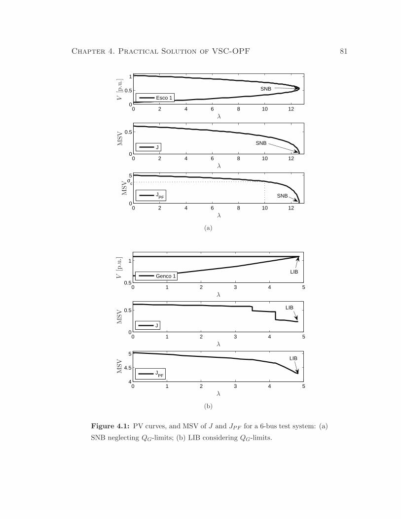
Chapter 4. Practical Solution of VSC-OPF 81
0 2 4 6 8 10 120
0.5
1
Esco 1
0 2 4 6 8 10 120
0.5
J
0 2 4 6 8 10 120
5
JPF
SNB
SNB
SNB
σc
λ
λ
λV
[p.u
.]M
SV
MSV
(a)
0 1 2 3 4 50.5
1
0 1 2 3 4 50
0.5
0 1 2 3 4 54
4.5
5
Genco 1
J
JPF
LIB
LIB
LIB
λ
λ
λ
V[p
.u.]
MSV
MSV
(b)
Figure 4.1: PV curves, and MSV of J and JPF for a 6-bus test system: (a)
SNB neglecting QG-limits; (b) LIB considering QG-limits.
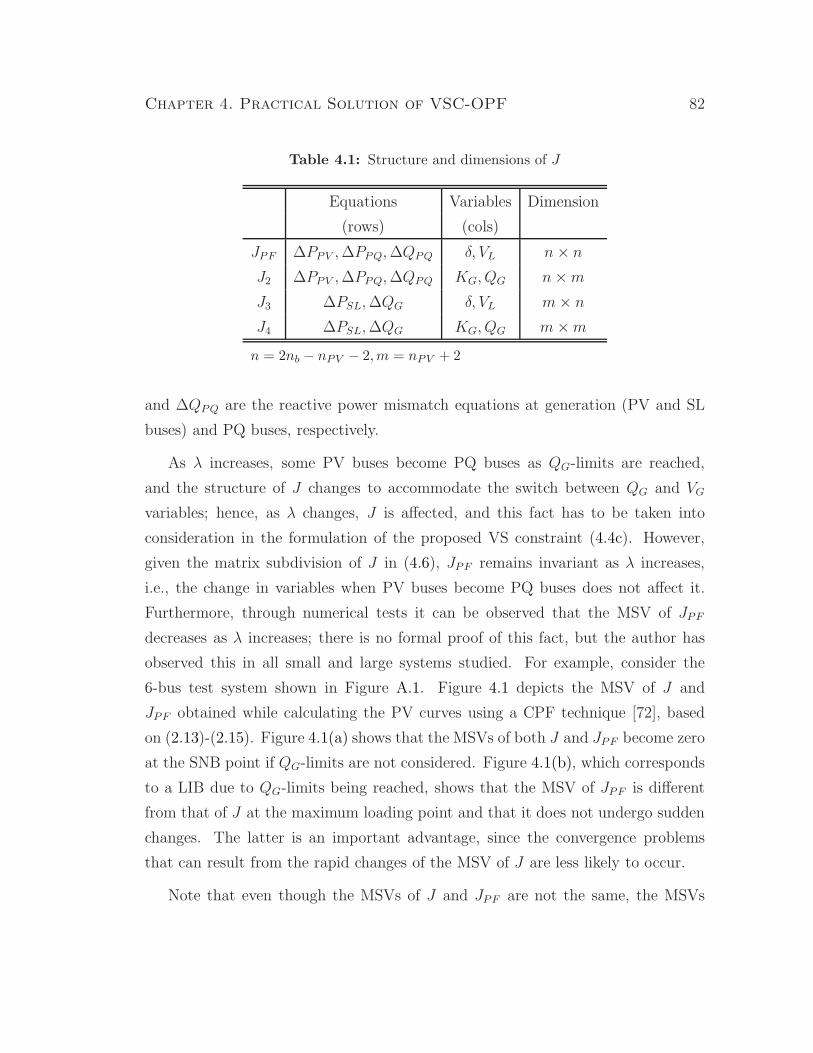
Chapter 4. Practical Solution of VSC-OPF 82
Table 4.1: Structure and dimensions of J
Equations Variables Dimension
(rows) (cols)
JPF ∆PPV , ∆PPQ, ∆QPQ δ, VL n× n
J2 ∆PPV , ∆PPQ, ∆QPQ KG, QG n×m
J3 ∆PSL, ∆QG δ, VL m× n
J4 ∆PSL, ∆QG KG, QG m×m
n = 2nb − nPV − 2,m = nPV + 2
and ∆QPQ are the reactive power mismatch equations at generation (PV and SL
buses) and PQ buses, respectively.
As λ increases, some PV buses become PQ buses as QG-limits are reached,
and the structure of J changes to accommodate the switch between QG and VG
variables; hence, as λ changes, J is affected, and this fact has to be taken into
consideration in the formulation of the proposed VS constraint (4.4c). However,
given the matrix subdivision of J in (4.6), JPF remains invariant as λ increases,
i.e., the change in variables when PV buses become PQ buses does not affect it.
Furthermore, through numerical tests it can be observed that the MSV of JPF
decreases as λ increases; there is no formal proof of this fact, but the author has
observed this in all small and large systems studied. For example, consider the
6-bus test system shown in Figure A.1. Figure 4.1 depicts the MSV of J and
JPF obtained while calculating the PV curves using a CPF technique [72], based
on (2.13)-(2.15). Figure 4.1(a) shows that the MSVs of both J and JPF become zero
at the SNB point if QG-limits are not considered. Figure 4.1(b), which corresponds
to a LIB due to QG-limits being reached, shows that the MSV of JPF is different
from that of J at the maximum loading point and that it does not undergo sudden
changes. The latter is an important advantage, since the convergence problems
that can result from the rapid changes of the MSV of J are less likely to occur.
Note that even though the MSVs of J and JPF are not the same, the MSVs
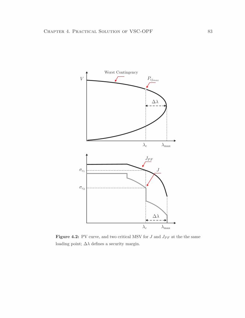
Chapter 4. Practical Solution of VSC-OPF 83
λc
λc
λmax
λmax
∆λ
∆λ
σc1
σc2
V
JPF
J
Pijmax
Worst Contingency
Figure 4.2: PV curve, and two critical MSV for J and JPF at the the same
loading point; ∆λ defines a security margin.

Chapter 4. Practical Solution of VSC-OPF 84
0 0.02 0.04 0.06 0.08 0.1 0.12 0.14 0.160.7
0.71
0.72
0.73
0.74
0.75
0.76
0.77
0.78
0.79
J
PF
λ
MSV
Figure 4.3: MSV of JPF for the CIGRE-32 test system considering QG-
limits.
of these Jacobians associated with any maximum loading point of interest can be
used as a VSI for a particular system. This is illustrated in a more general form
in Figure 4.2, where σc1 or σc2 define a “critical” MSV of a particular system
at certain loading point defined by λc; these values are chosen off-line, so that
λc defines a maximum loading point for a given dispatch pattern considering the
worst contingency. It should be mentioned that the MSV of JPF does not necessary
become zero at the SNB point when QG-limits are considered, as observed in studies
of larger test systems (e.g., the CIGRE-32 test system case shown in Figure 4.3).
However, as illustrated in Figure 4.2, the MSV of JPF simply defines an alternative
VSI that can be used to determine the σc value, which is a valid value from the
practical perspective of applying the proposed VSC-OPF.
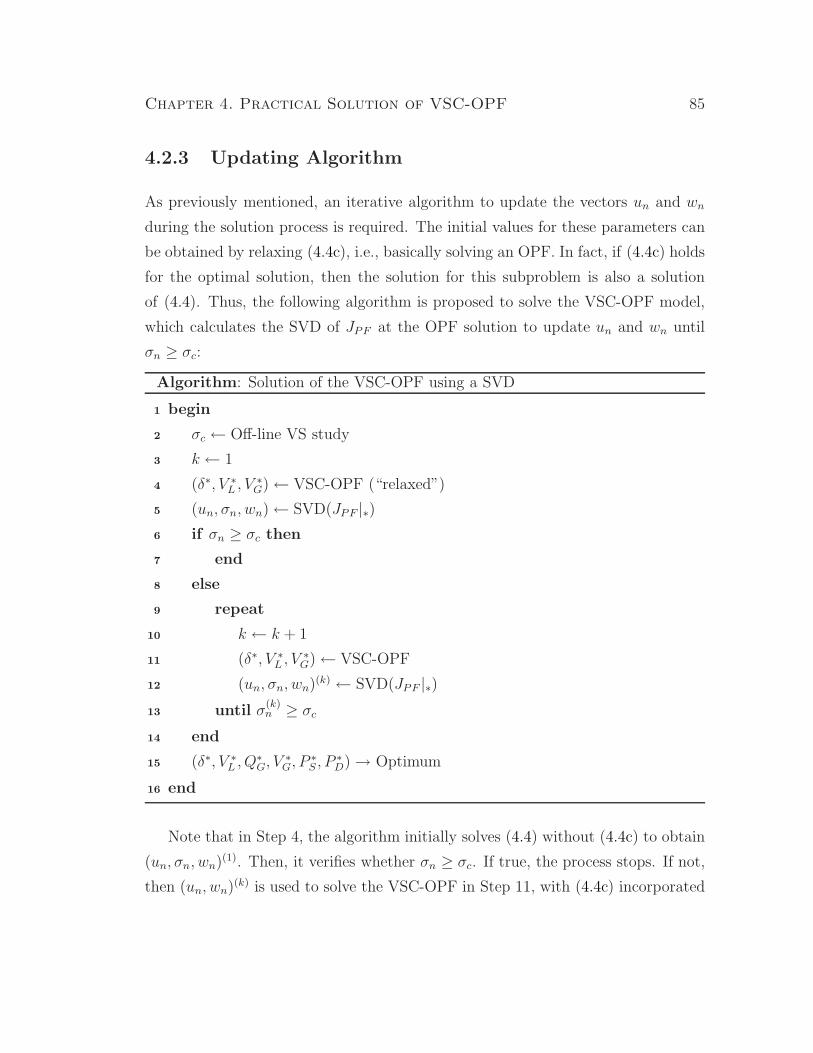
Chapter 4. Practical Solution of VSC-OPF 85
4.2.3 Updating Algorithm
As previously mentioned, an iterative algorithm to update the vectors un and wn
during the solution process is required. The initial values for these parameters can
be obtained by relaxing (4.4c), i.e., basically solving an OPF. In fact, if (4.4c) holds
for the optimal solution, then the solution for this subproblem is also a solution
of (4.4). Thus, the following algorithm is proposed to solve the VSC-OPF model,
which calculates the SVD of JPF at the OPF solution to update un and wn until
σn ≥ σc:
Algorithm: Solution of the VSC-OPF using a SVD
begin1
σc ← Off-line VS study2
k ← 13
(δ∗, V ∗L , V ∗
G)← VSC-OPF (“relaxed”)4
(un, σn, wn)← SVD(JPF |∗)5
if σn ≥ σc then6
end7
else8
repeat9
k ← k + 110
(δ∗, V ∗L , V ∗
G)← VSC-OPF11
(un, σn, wn)(k) ← SVD(JPF |∗)12
until σ(k)n ≥ σc13
end14
(δ∗, V ∗L , Q∗
G, V ∗G, P ∗
S , P ∗D)→ Optimum15
end16
Note that in Step 4, the algorithm initially solves (4.4) without (4.4c) to obtain
(un, σn, wn)(1). Then, it verifies whether σn ≥ σc. If true, the process stops. If not,
then (un, wn)(k) is used to solve the VSC-OPF in Step 11, with (4.4c) incorporated

Chapter 4. Practical Solution of VSC-OPF 86
into the optimization. The SVD is updated at the new solution, and k is increased.
The process is repeated until σ(k)n ≥ σc.
4.3 Numerical Results
This section presents and discusses numerical examples of the proposed method,
concentrating first on demonstrating how the proposed VSC-OPF method (4.4)
works, and comparing it to the VSC-OPF model (2.24). A comparison between the
VSC-OPF (4.4) and the SC-OPF (2.21) is then presented to study the effect of the
proposed VS constraint on a single 6-bus model. Finally, a 1211-bus system model
representing an actual European network is used to demonstrate the feasibility of
applying the proposed technique in practice.
The proposed method (4.4) was formulated using the AMPL [93] modeling
language and solved with IPOPT [98], whereas Matlab [99] was used for the required
SVD computations. The optimization model (2.24) was implemented in Matlab,
since current mathematical programming languages are not able to handle implicit
constraints.
4.3.1 Effect of Proposed VS Constraint
A numerical example to illustrate the application of the proposed method and the
effect of σc on the results is presented here using the 6-bus test system shown in
Figure A.1. Observe in Figure 4.1(b) that a small change in σc for this system,
e.g., from 4.99 to 5.03, can have a significant effect on the loading margin (security
levels), hence affecting system dispatch levels and market conditions.
Table 4.2 shows the initial values of un and wn obtained at each iteration of
the proposed method. Notice the progress of σn with respect to the values chosen
for σc, with the starting system conditions meeting the initial value chosen for
σc1 = 4.99 (in this case the proposed method did not require any iterations), and

Chapter 4. Practical Solution of VSC-OPF 87
Table 4.2: Progress of the unitary vectors and MSV when σc is increased
from 4.99 to 5.03.
Initial values k = 1 k = 2
u(0)n w
(0)n u
(1)n w
(1)n u
(2)n w
(2)n
-0.3504 0.3556 -0.3535 0.3583 -0.3535 0.3583
-0.5266 0.5377 -0.5275 0.5375 -0.5275 0.5376
-0.2540 0.2426 -0.2557 0.2447 -0.2557 0.2448
-0.5102 0.4879 -0.5078 0.4879 -0.5055 0.4878
-0.5242 0.5167 -0.5227 0.5161 -0.5228 0.5162
0.0076 0.0659 0.0100 0.0642 0.0101 0.0642
-0.0019 0.0993 0.0043 0.0936 0.0045 0.0934
0.0086 0.0784 0.0131 0.0742 0.0132 0.0741
σ(0)n = 4.99 ≥ 4.99 σ
(1)n = 5.0291 < 5.03 σ
(2)n = 5.0302 > 5.03
Table 4.3: Comparison of voltage, power dispatch, and LMPs at the solu-
tion of the VSC-OPF when σc is increased from 4.99 to 5.03.
Participant
VSC-OPF (σc = 4.99) VSC-OPF (σc = 5.0302)
V PS/PD LMP V PS/PD LMP
[p.u.] [MW] [$/MWh] [p.u.] [MW] [$/MWh]
GENCO 1 1.1 0 8.95 1.1 0 9.06
GENCO 2 1.1 25 8.90 1.1 6.0 8.80
GENCO 3 1.1 20 9.07 1.1 20 9.33
ESCO 1 1.021 25 9.48 1.022 25 9.60
ESCO 2 1.012 10 9.58 1.020 0.85 9.98
ESCO 3 1.038 8.0 9.35 1.044 0 9.73
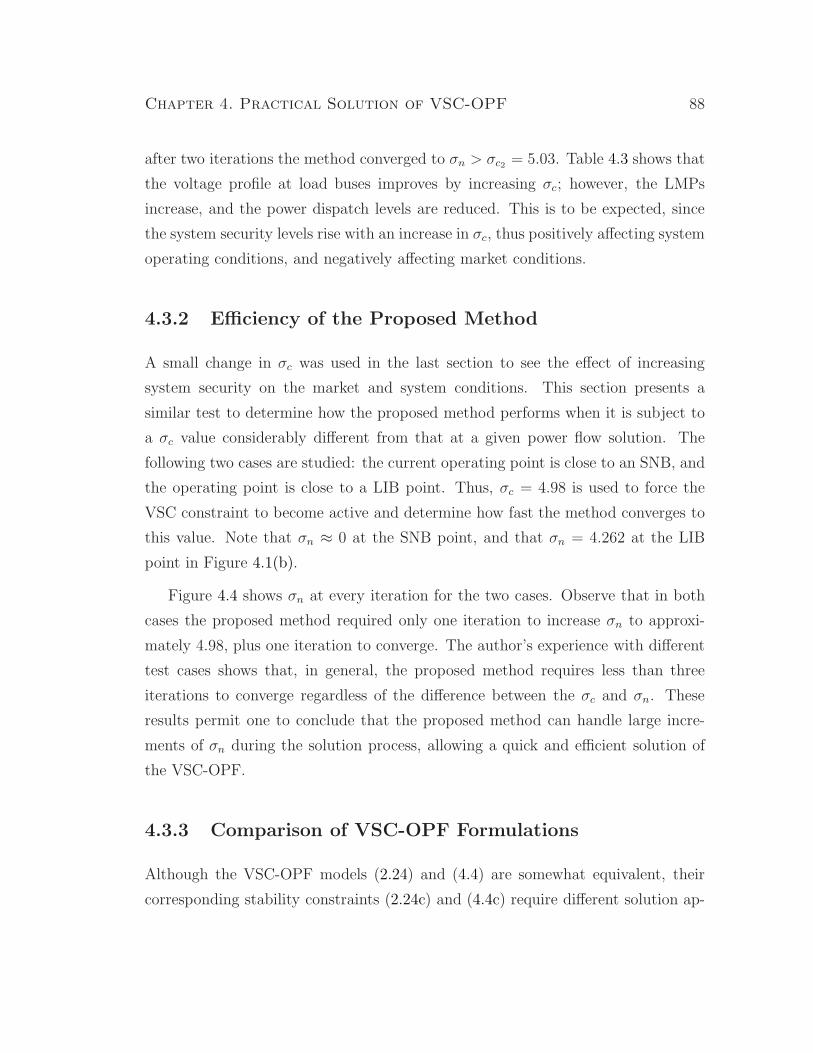
Chapter 4. Practical Solution of VSC-OPF 88
after two iterations the method converged to σn > σc2 = 5.03. Table 4.3 shows that
the voltage profile at load buses improves by increasing σc; however, the LMPs
increase, and the power dispatch levels are reduced. This is to be expected, since
the system security levels rise with an increase in σc, thus positively affecting system
operating conditions, and negatively affecting market conditions.
4.3.2 Efficiency of the Proposed Method
A small change in σc was used in the last section to see the effect of increasing
system security on the market and system conditions. This section presents a
similar test to determine how the proposed method performs when it is subject to
a σc value considerably different from that at a given power flow solution. The
following two cases are studied: the current operating point is close to an SNB, and
the operating point is close to a LIB point. Thus, σc = 4.98 is used to force the
VSC constraint to become active and determine how fast the method converges to
this value. Note that σn ≈ 0 at the SNB point, and that σn = 4.262 at the LIB
point in Figure 4.1(b).
Figure 4.4 shows σn at every iteration for the two cases. Observe that in both
cases the proposed method required only one iteration to increase σn to approxi-
mately 4.98, plus one iteration to converge. The author’s experience with different
test cases shows that, in general, the proposed method requires less than three
iterations to converge regardless of the difference between the σc and σn. These
results permit one to conclude that the proposed method can handle large incre-
ments of σn during the solution process, allowing a quick and efficient solution of
the VSC-OPF.
4.3.3 Comparison of VSC-OPF Formulations
Although the VSC-OPF models (2.24) and (4.4) are somewhat equivalent, their
corresponding stability constraints (2.24c) and (4.4c) require different solution ap-
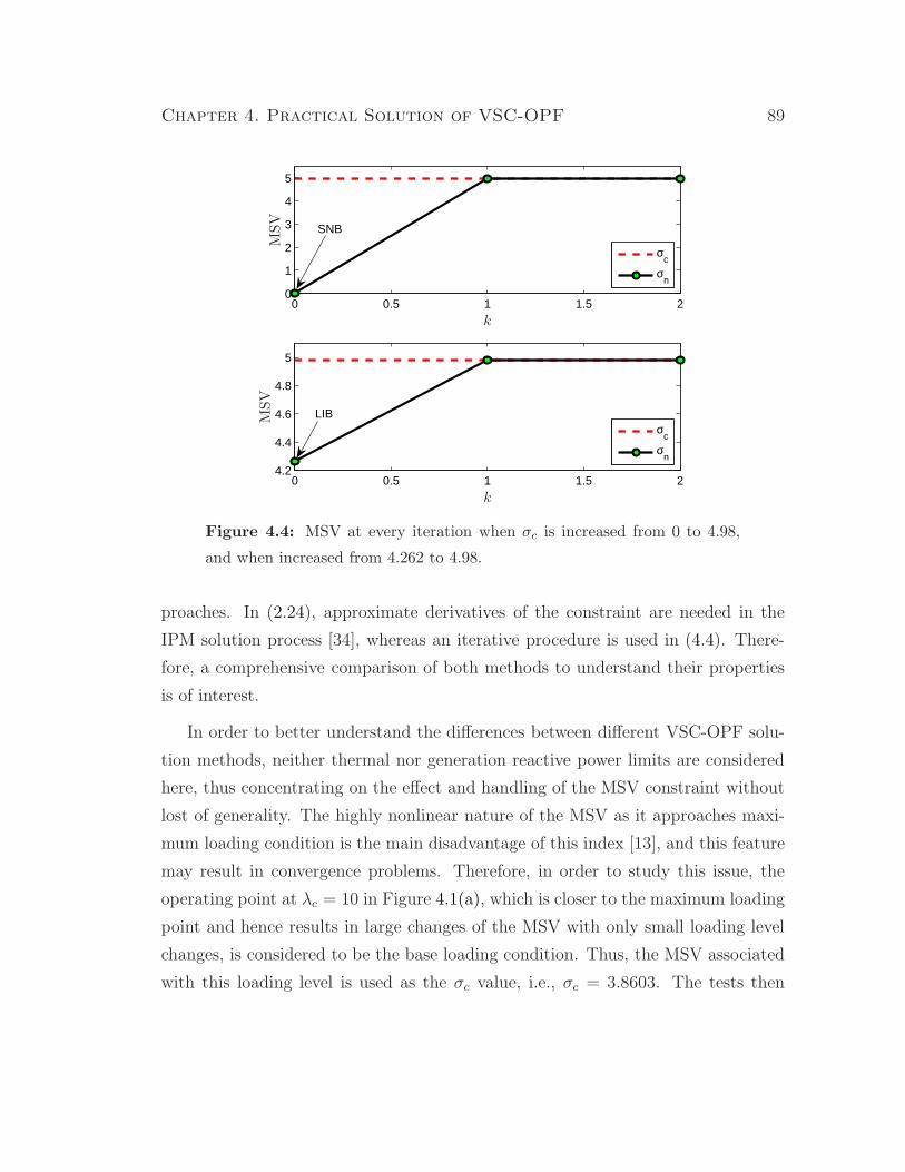
Chapter 4. Practical Solution of VSC-OPF 89
0 0.5 1 1.5 20
1
2
3
4
5
0 0.5 1 1.5 24.2
4.4
4.6
4.8
5
σc
σn
σc
σn
SNB
LIB
k
k
MSV
MSV
Figure 4.4: MSV at every iteration when σc is increased from 0 to 4.98,
and when increased from 4.262 to 4.98.
proaches. In (2.24), approximate derivatives of the constraint are needed in the
IPM solution process [34], whereas an iterative procedure is used in (4.4). There-
fore, a comprehensive comparison of both methods to understand their properties
is of interest.
In order to better understand the differences between different VSC-OPF solu-
tion methods, neither thermal nor generation reactive power limits are considered
here, thus concentrating on the effect and handling of the MSV constraint without
lost of generality. The highly nonlinear nature of the MSV as it approaches maxi-
mum loading condition is the main disadvantage of this index [13], and this feature
may result in convergence problems. Therefore, in order to study this issue, the
operating point at λc = 10 in Figure 4.1(a), which is closer to the maximum loading
point and hence results in large changes of the MSV with only small loading level
changes, is considered to be the base loading condition. Thus, the MSV associated
with this loading level is used as the σc value, i.e., σc = 3.8603. The tests then
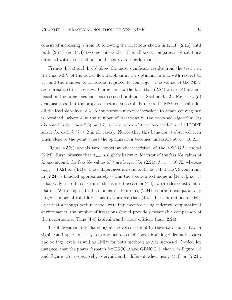
Chapter 4. Practical Solution of VSC-OPF 90
consist of increasing λ from 10 following the directions shown in (2.13)-(2.15) until
both (2.24) and (4.4) become unfeasible. This allows a comparison of solutions
obtained with these methods and their overall performance.
Figures 4.5(a) and 4.5(b) show the most significant results from the test, i.e.,
the final MSV of the power flow Jacobian at the optimum in p.u. with respect to
σc, and the number of iterations required to converge. The values of the MSV
are normalized in these two figures due to the fact that (2.24) and (4.4) are not
based on the same Jacobian (as discussed in detail in Section 4.2.2). Figure 4.5(a)
demonstrates that the proposed method successfully meets the MSV constraint for
all the feasible values of λ. A consistent number of iterations to attain convergence
is obtained, where k is the number of iterations in the proposed algorithm (as
discussed in Section 4.2.3), and ks is the number of iterations needed by the IPOPT
solver for each k (k ≤ 2 in all cases). Notice that this behavior is observed even
when close to the point where the optimization becomes unfeasible at λ = 10.21.
Figure 4.5(b) reveals two important characteristics of the VSC-OPF model
(2.24). First, observe that σmin is slightly below σc for most of the feasible values of
λ; and second, the feasible values of λ are larger (for (2.24), λmax = 10.72, whereas
λmax = 10.21 for (4.4)). These differences are due to the fact that the VS constraint
in (2.24) is handled approximately within the solution technique in [34, 45], i.e., it
is basically a “soft” constraint; this is not the case in (4.4), where this constraint is
“hard”. With respect to the number of iterations, (2.24) requires a comparatively
larger number of total iterations to converge than (4.4). It is important to high-
light that although both methods were implemented using different computational
environments, the number of iterations should provide a reasonable comparison of
the performance. Thus (4.4) is significantly more efficient than (2.24).
The differences in the handling of the VS constraint by these two models have a
significant impact in the system and market conditions, obtaining different dispatch
and voltage levels as well as LMPs for both methods as λ is increased. Notice, for
instance, that the power dispatch for ESCO 3 and GENCO 3, shown in Figure 4.6
and Figure 4.7, respectively, is significantly different when using (4.4) or (2.24).

Chapter 4. Practical Solution of VSC-OPF 91
10 10.05 10.1 10.15 10.21
1.0001
1.0002
1.0003
10 10.05 10.1 10.15 10.20
5
10
15
kk
s
σn
σc
λ
λ
MSV
[p.u
.]
Iter
ations
(a)
10 10.1 10.2 10.3 10.4 10.5 10.6 10.70.9
1
1.1
1.2
1.3
10 10.1 10.2 10.3 10.4 10.5 10.6 10.70
200
400
600
σmin
σc
λ
λ
MSV
[p.u
.]It
erations
(b)
Figure 4.5: MSV at the optimum with respect to the loading factor (a)
for (4.4), and (b) for (2.24).

Chapter 4. Practical Solution of VSC-OPF 92
10 10.1 10.2 10.3 10.4 10.5 10.6 10.70
0.02
0.04
0.06
0.08
0.1
0.12
0.14
0.16
PD3
: VSC−OPF (4.4)
PD3
: VSC−OPF (2.24)
λ
PD
[p.u
.]
Figure 4.6: ESCO 3 power with respect to the loading factor for the 6-bus
system.
10 10.1 10.2 10.3 10.4 10.5 10.6 10.70
0.02
0.04
0.06
0.08
0.1
0.12
0.14
0.16
0.18
0.2
P
S3: VSC−OPF (4.4)
PS3
: VSC−OPF (2.24)
λ
PS
[p.u
.]
Figure 4.7: GENCO 3 power with respect to the loading factor for the
6-bus system.
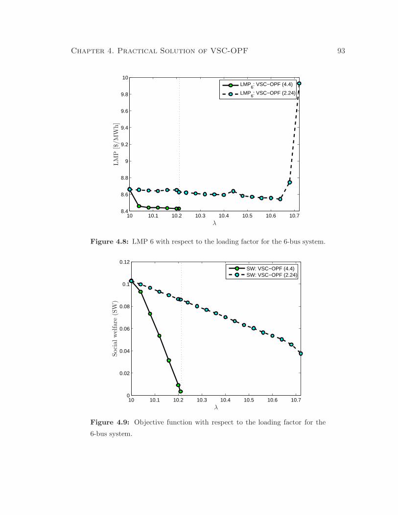
Chapter 4. Practical Solution of VSC-OPF 93
10 10.1 10.2 10.3 10.4 10.5 10.6 10.78.4
8.6
8.8
9
9.2
9.4
9.6
9.8
10
LMP
6: VSC−OPF (4.4)
LMP6: VSC−OPF (2.24)
λ
LM
P[$
/M
Wh]
Figure 4.8: LMP 6 with respect to the loading factor for the 6-bus system.
10 10.1 10.2 10.3 10.4 10.5 10.6 10.70
0.02
0.04
0.06
0.08
0.1
0.12
SW: VSC−OPF (4.4)SW: VSC−OPF (2.24)
λ
Soci
alw
elfa
re(S
W)
Figure 4.9: Objective function with respect to the loading factor for the
6-bus system.
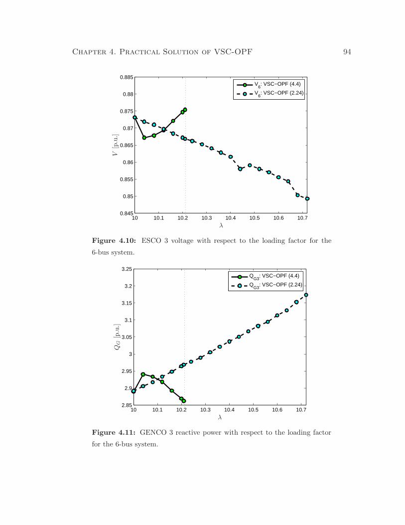
Chapter 4. Practical Solution of VSC-OPF 94
10 10.1 10.2 10.3 10.4 10.5 10.6 10.70.845
0.85
0.855
0.86
0.865
0.87
0.875
0.88
0.885
V
6: VSC−OPF (4.4)
V6: VSC−OPF (2.24)
λ
V[p
.u.]
Figure 4.10: ESCO 3 voltage with respect to the loading factor for the
6-bus system.
10 10.1 10.2 10.3 10.4 10.5 10.6 10.72.85
2.9
2.95
3
3.05
3.1
3.15
3.2
3.25
Q
G3: VSC−OPF (4.4)
QG3
: VSC−OPF (2.24)
λ
QG
[p.u
.]
Figure 4.11: GENCO 3 reactive power with respect to the loading factor
for the 6-bus system.

Chapter 4. Practical Solution of VSC-OPF 95
This difference is reflected in the corresponding LMP shown in Figure 4.8. The
social welfare depicted in Figure 4.9 shows that the power dispatch obtained us-
ing (4.4) is practically zero at the maximum loading point. This result permits one
to conclude that the proposed model tends to reduce the dispatchable loads in or-
der to satisfy the VS constraint until it becomes unfeasible. In contrast, the model
(2.24) continues to dispatch power until it becomes unfeasible due to convergence
problems, as concluded from the large number of iterations shown in Figure 4.5(b).
Notice that Figure 4.10 is in accordance with the differences in the market con-
ditions, i.e., the voltage increases at the buses where the power dispatch is reduced
using (4.4) as expected, since the VS constraint is closely related to the voltage lev-
els. Similarly, Figure 4.11 corroborates that the proposed model tends to reduce the
dispatchable loads when the system is under stressed security conditions, since re-
active power is still available. However, the proposed model is also able to readjust
other control variables when the load is inelastic, as discussed in Section 4.3.5.
4.3.4 Proposed VSC-OPF vs SC-OPF
The results presented in the previous section demonstrate that the proposed method
successfully and efficiently guarantees the required VS constraint. This section
presents a comparison between the VSC-OPF model (4.4) and the SC-OPF model
(2.21) to study how the corresponding VS constraint affects both the system and
market conditions.
The stability limits Pijmax in (2.21) were obtained by means of off-line maxi-
mum loadability analysis using a CPF method and considering an N-1 contingency
criterion. At the same time, σc in (4.4) corresponds to the value of σmin(JPF ) at
the same loading level λc corresponding to Pijmax.
The results presented in Tables 4.4 and 4.5 correspond to the solution of the
SC-OPF as well as the proposed VSC-OPF models at the base loading condition,
respectively. This comparison shows that the VSC-OPF auction model provides
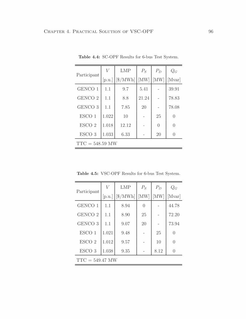
Chapter 4. Practical Solution of VSC-OPF 96
Table 4.4: SC-OPF Results for 6-bus Test System.
ParticipantV LMP PS PD QG
[p.u.] [$/MWh] [MW] [MW] [Mvar]
GENCO 1 1.1 9.7 5.41 - 39.91
GENCO 2 1.1 8.8 21.24 - 78.83
GENCO 3 1.1 7.85 20 - 78.08
ESCO 1 1.022 10 - 25 0
ESCO 2 1.018 12.12 - 0 0
ESCO 3 1.033 6.33 - 20 0
TTC = 548.59 MW
Table 4.5: VSC-OPF Results for 6-bus Test System.
ParticipantV LMP PS PD QG
[p.u.] [$/MWh] [MW] [MW] [Mvar]
GENCO 1 1.1 8.94 0 - 44.78
GENCO 2 1.1 8.90 25 - 72.20
GENCO 3 1.1 9.07 20 - 73.94
ESCO 1 1.021 9.48 - 25 0
ESCO 2 1.012 9.57 - 10 0
ESCO 3 1.038 9.35 - 8.12 0
TTC = 549.47 MW

Chapter 4. Practical Solution of VSC-OPF 97
lower and more uniform LMPs than the SC-OPF; furthermore, the TTC level
obtained using a continuation method and the corresponding dispatch directions
in (2.13)-(2.15) are slightly higher than in the SC-OPF. These results show that
the VSC-OPF yields better market and system conditions than the SC-OPF, while
meeting the required security constraints. Thus, the proposed representation of
system security is better overall than simply using fixed limits on power flows.
The base loading level was then increased following the power directions shown
in (2.13)-(2.15) to determine the maximum feasible point of these two models. For
these studies, the differences in the power dispatch at every bus for both models
are shown in Figures 4.12-4.14, for ESCOs, and in Figures 4.15-4.17, for GENCOs.
These figures show that the use of a more “relaxed” stability constraint in the
proposed VSC-OPF than in the SC-OPF yields higher dispatch levels and conse-
quently better objective function values, as shown in Figure 4.18. Observe that
the maximum feasible point for both models occurs at λ = λc = 1.98, as expected,
since this value corresponds to the loading level defining Pijmax and σc. However,
notice also that the dispatch in the SC-OPF starts to decrease earlier than in the
VSC-OPF, becoming practically zero at λc. Figures 4.19-4.24 show that the LMPs
obtained using the VSC-OPF have a better profile than the LMPs obtained using
the SC-OPF as the load increases, as expected from the results shown in Tables 4.4
and 4.5. Observe the drastic change in the LMP values as these models approach
the maximum feasible point.
Observe in Figures 4.25 and 4.26 (corresponding to the most representative buses
as well) that the bus voltage levels are within limits, and more reactive power can
be supplied. However, the lower voltage and higher reactive power values obtained
in the VSC-OPF indicate that this model allows a greater power supply than in
the SC-OPF within the same operational limits.
Figure 4.27 shows the MSV for both SC-OPF and VSC-OPF, as well as the value
of σc used in (4.4). Observe that the MSV constraint in the VSC-OPF becomes
active at λ = 1.6. Furthermore, the SC-OPF is shown to be more secure than
the VSC-OPF as the loading increases, since its corresponding σmin value is higher
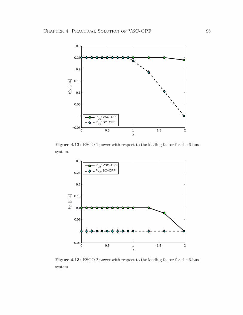
Chapter 4. Practical Solution of VSC-OPF 98
0 0.5 1 1.5 2−0.05
0
0.05
0.1
0.15
0.2
0.25
0.3
PD1
: VSC−OPF
PD1
: SC−OPF
λ
PD
[p.u
.]
Figure 4.12: ESCO 1 power with respect to the loading factor for the 6-bus
system.
0 0.5 1 1.5 2−0.05
0
0.05
0.1
0.15
0.2
0.25
0.3
P
D2: VSC−OPF
PD2
: SC−OPF
λ
PD
[p.u
.]
Figure 4.13: ESCO 2 power with respect to the loading factor for the 6-bus
system.

Chapter 4. Practical Solution of VSC-OPF 99
0 0.5 1 1.5 2−0.05
0
0.05
0.1
0.15
0.2
0.25
0.3
P
D3: VSC−OPF
PD3
: SC−OPF
λ
PD
[p.u
.]
Figure 4.14: ESCO 3 power with respect to the loading factor for the 6-bus
system.
0 0.5 1 1.5 20
0.05
0.1
0.15
0.2
0.25
P
S1: VSC−OPF
PS1
: SC−OPF
λ
PS
[p.u
.]
Figure 4.15: GENCO 1 power with respect to the loading factor for the
6-bus system.
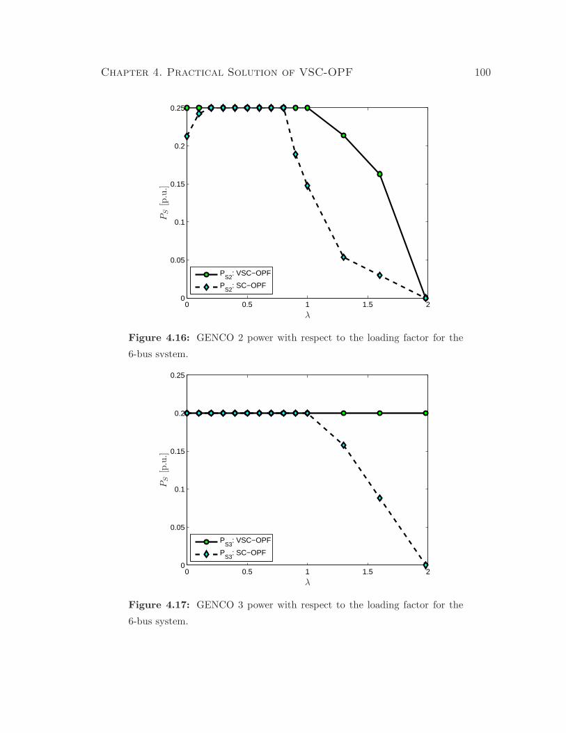
Chapter 4. Practical Solution of VSC-OPF 100
0 0.5 1 1.5 20
0.05
0.1
0.15
0.2
0.25
PS2
: VSC−OPF
PS2
: SC−OPF
λ
PS
[p.u
.]
Figure 4.16: GENCO 2 power with respect to the loading factor for the
6-bus system.
0 0.5 1 1.5 20
0.05
0.1
0.15
0.2
0.25
PS3
: VSC−OPF
PS3
: SC−OPF
λ
PS
[p.u
.]
Figure 4.17: GENCO 3 power with respect to the loading factor for the
6-bus system.

Chapter 4. Practical Solution of VSC-OPF 101
0 0.5 1 1.5 2−0.2
0
0.2
0.4
0.6
0.8
1
1.2
1.4
SW: VSC−OPFSW: SC−OPF
λ
Soci
alw
elfa
re(S
W)
Figure 4.18: Objective function with respect to the loading factor for the
6-bus system.
0 0.5 1 1.5 2
2
4
6
8
10
12
14
LMP1: VSC−OPF
LMP1: SC−OPF
λ
LM
P[$
/M
Wh]
Figure 4.19: Locational Marginal Price (LMP) at bus 1 with respect to
the loading factor for the 6-bus system.
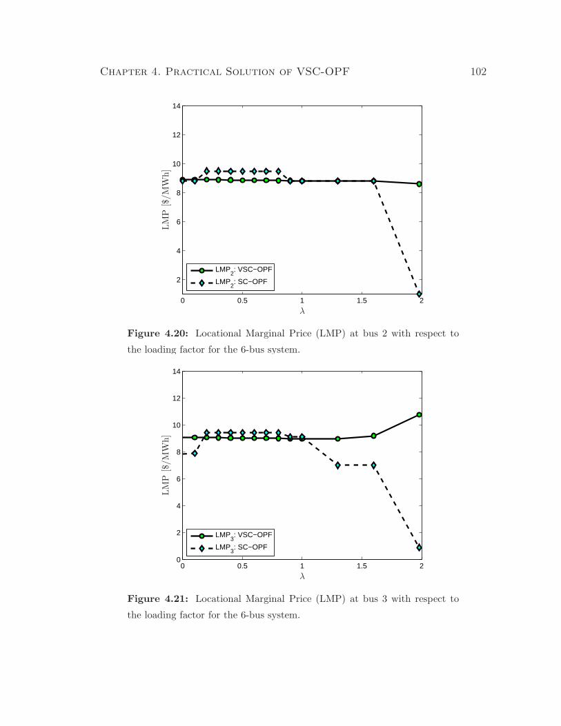
Chapter 4. Practical Solution of VSC-OPF 102
0 0.5 1 1.5 2
2
4
6
8
10
12
14
LMP2: VSC−OPF
LMP2: SC−OPF
λ
LM
P[$
/M
Wh]
Figure 4.20: Locational Marginal Price (LMP) at bus 2 with respect to
the loading factor for the 6-bus system.
0 0.5 1 1.5 20
2
4
6
8
10
12
14
LMP3: VSC−OPF
LMP3: SC−OPF
λ
LM
P[$
/M
Wh]
Figure 4.21: Locational Marginal Price (LMP) at bus 3 with respect to
the loading factor for the 6-bus system.
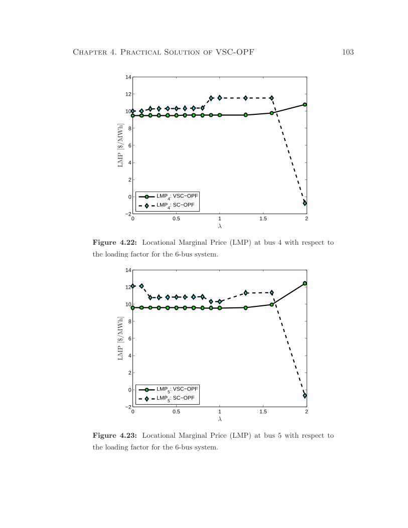
Chapter 4. Practical Solution of VSC-OPF 103
0 0.5 1 1.5 2−2
0
2
4
6
8
10
12
14
LMP4: VSC−OPF
LMP4: SC−OPF
λ
LM
P[$
/M
Wh]
Figure 4.22: Locational Marginal Price (LMP) at bus 4 with respect to
the loading factor for the 6-bus system.
0 0.5 1 1.5 2−2
0
2
4
6
8
10
12
14
LMP5: VSC−OPF
LMP5: SC−OPF
λ
LM
P[$
/M
Wh]
Figure 4.23: Locational Marginal Price (LMP) at bus 5 with respect to
the loading factor for the 6-bus system.
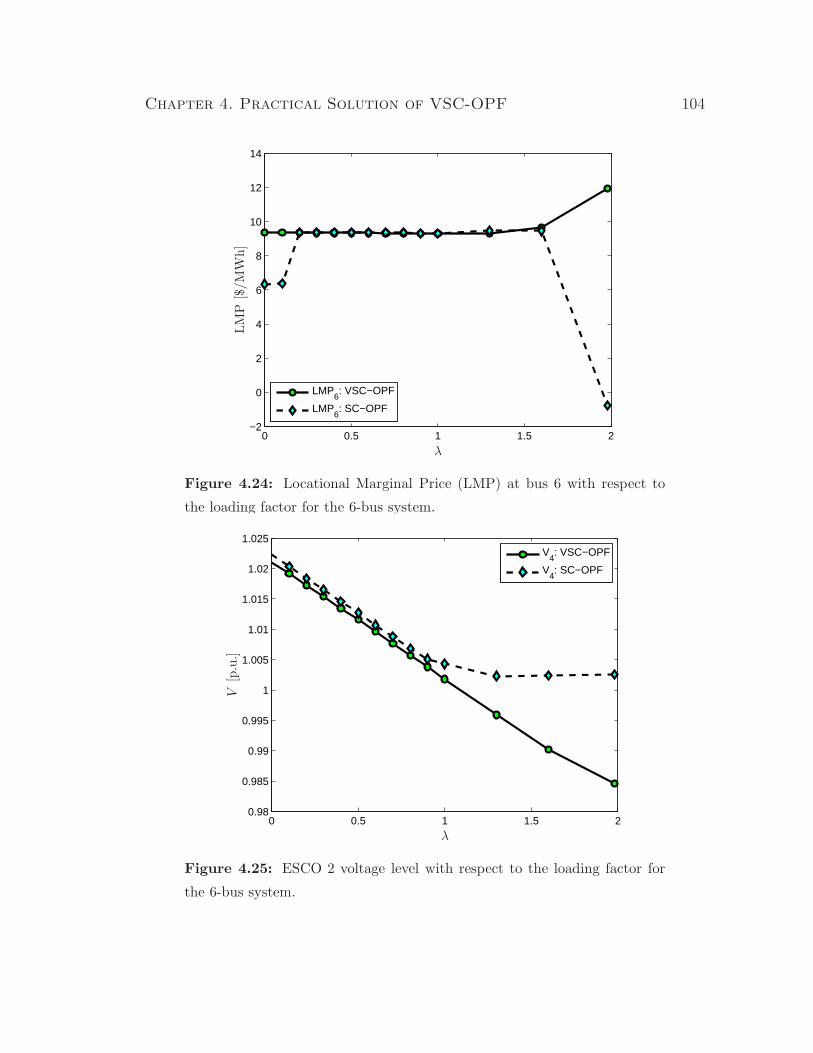
Chapter 4. Practical Solution of VSC-OPF 104
0 0.5 1 1.5 2−2
0
2
4
6
8
10
12
14
LMP6: VSC−OPF
LMP6: SC−OPF
λ
LM
P[$
/M
Wh]
Figure 4.24: Locational Marginal Price (LMP) at bus 6 with respect to
the loading factor for the 6-bus system.
0 0.5 1 1.5 20.98
0.985
0.99
0.995
1
1.005
1.01
1.015
1.02
1.025
V
4: VSC−OPF
V4: SC−OPF
λ
V[p
.u.]
Figure 4.25: ESCO 2 voltage level with respect to the loading factor for
the 6-bus system.

Chapter 4. Practical Solution of VSC-OPF 105
0 0.5 1 1.5 20.7
0.8
0.9
1
1.1
1.2
1.3
1.4
Q
G2: VSC−OPF
QG2
: SC−OPF
λ
QG
[p.u
.]
Figure 4.26: GENCO 2 reactive power with respect to the loading factor
for the 6-bus system.
0 0.5 1 1.5 24.9
4.91
4.92
4.93
4.94
4.95
4.96
4.97
4.98
4.99
5
σ
min: VSC−OPF
σmin
: SC−OPF
σc = 4.9025
λ
MSV
Figure 4.27: MSV at the optimum of the VSC-OPF and SC-OPF.

Chapter 4. Practical Solution of VSC-OPF 106
0 0.5 1 1.5 21
1.1
1.2
1.3
1.4
1.5
1.6
1.7
1.8
1.9
2
ATC: VSC−OPFATC: SC−OPF
λ
AT
C[p
.u.]
Figure 4.28: ATC with respect to system loading for the 6-bus system.
0 0.5 1 1.5 25.465
5.47
5.475
5.48
5.485
5.49
5.495
5.5
5.505
TTC: VSC−OPFTTC: SC−OPF
λ
TT
C[p
.u.]
Figure 4.29: TTC with respect to system loading for the 6-bus system.
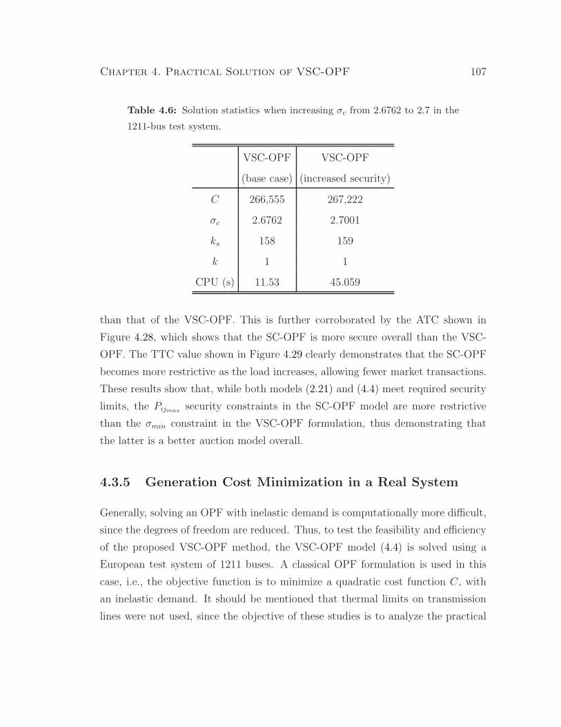
Chapter 4. Practical Solution of VSC-OPF 107
Table 4.6: Solution statistics when increasing σc from 2.6762 to 2.7 in the
1211-bus test system.
VSC-OPF VSC-OPF
(base case) (increased security)
C 266,555 267,222
σc 2.6762 2.7001
ks 158 159
k 1 1
CPU (s) 11.53 45.059
than that of the VSC-OPF. This is further corroborated by the ATC shown in
Figure 4.28, which shows that the SC-OPF is more secure overall than the VSC-
OPF. The TTC value shown in Figure 4.29 clearly demonstrates that the SC-OPF
becomes more restrictive as the load increases, allowing fewer market transactions.
These results show that, while both models (2.21) and (4.4) meet required security
limits, the Pijmax security constraints in the SC-OPF model are more restrictive
than the σmin constraint in the VSC-OPF formulation, thus demonstrating that
the latter is a better auction model overall.
4.3.5 Generation Cost Minimization in a Real System
Generally, solving an OPF with inelastic demand is computationally more difficult,
since the degrees of freedom are reduced. Thus, to test the feasibility and efficiency
of the proposed VSC-OPF method, the VSC-OPF model (4.4) is solved using a
European test system of 1211 buses. A classical OPF formulation is used in this
case, i.e., the objective function is to minimize a quadratic cost function C, with
an inelastic demand. It should be mentioned that thermal limits on transmission
lines were not used, since the objective of these studies is to analyze the practical

Chapter 4. Practical Solution of VSC-OPF 108
0 200 400 600 800 1000 1200−1200
−1000
−800
−600
−400
−200
0
200
400
600
Bus
∆P
G[M
W]
Figure 4.30: Generation re-dispatch when the VSC-OPF is applied to a
1211-bus test system.
0 200 400 600 800 1000 1200−0.02
−0.01
0
0.01
0.02
0.03
0.04
0.05
0.06
Bus
∆V
[p.u
.]
Figure 4.31: Increment in bus voltages when the VSC-OPF is applied to a
1211-bus test system.

Chapter 4. Practical Solution of VSC-OPF 109
feasibility and performance of the proposed VSC-OPF. Thus, the VSC-OPF (4.4)
was solved first under normal operating conditions without the MSV constraint
(base case), and a σmin(JPF ) was obtained for this solution. Then, to force the
MSV constraint (4.4c) to become active, a slightly larger value than σmin was used
as the σc value in the solution of (4.4).
Figure 4.30 shows that a generation re-dispatch with respect to the base case
solution is required to meet the required security constraint, improving the voltage
profile at most of the buses, as expected and depicted in Figure 4.31. However,
this corrective action is accompanied by an increase in the total generation costs,
as shown in Table 4.6; this increase in the total cost can be seen as the cost of
improving system security.
The results presented in Table 4.6 demonstrate the feasibility of the proposed
method in practice, since for this large system, it only required one iteration and
45s of CPU time for the method to converge using a (Intel Xeon 2.83GHz with
3.00 GB of RAM). In general, the author’s experience with different test systems
shows that the proposed method converges in less than three iterations (k ≤ 3),
regardless of the system size.

Chapter 4. Practical Solution of VSC-OPF 110
4.4 Summary
In this chapter, a novel and practical solution method to solve a VSC-OPF model
that includes a VS constraint based on a MSV index is proposed. The method
consists of solving the VSC-OPF iteratively to update the SVD of the power flow
Jacobian until the MSV constraint is satisfied. The proposed method is shown to
have better numerical characteristics than a previously proposed VSC-OPF model
based on a similar VS constraint.
The advantages of using the proposed method with respect to “standard” SC-
OPF are highlighted by means of numerical comparisons. In this context, it is
demonstrated that the VSC-OPF model provides better system and market con-
ditions when compared to the SC-OPF. It is shown that the proposed method
performs well in large systems, demonstrating its practical feasibility by applying
it to a real European system. One of the main advantages of the proposed model
is that commercial mathematical programming languages and solvers can be used
to formulate it, making it easier to implement and more practical. Overall, the
proposed method is shown to be a good alternative to SC-OPFs.

Chapter 5
Other Approaches to Solving the
VSC-OPF
5.1 Introduction
This chapter proposes two alternative methods to solving the MSV-based VSC-OPF
model, besides the method discussed in the previous chapter. The first method is a
modified primal-dual IPM which handles the MSV constraint using a CP technique
at every iteration. The second method attempts to reformulate the VSC-OPF as a
SDP relaxation.
5.2 Solving the VSC-OPF via CP/IPM
Although the CP method is commonly used to solve mixed-integer problems in
linear programming, the basic idea of adding linear constraints (cuts) until the op-
timal solution reaches desired values is extended here to solve the VSC-OPF. Thus,
a modified primal-dual IPM algorithm is proposed in this section to incorporate
a CP step to modify the upper limits of the demand block bids at a particular
111

Chapter 5. Other Approaches to Solving the VSC-OPF 112
Feasibility of power flow
equations within 10 .-3
Feasible region
Original central path
cut
New central path direction
replacemen
x(0)
x(1)
x(2) x(3)
x(4)
σmin(JPF ) < σc
σmin(JPF ) < σc
x(5)
x∗∗, σmin(JPF ) ≥ σc
x∗, σmin(JPF ) < σc
∆x(0)
∆x(1)
∆x(2)
∆x(3)∆x(4)
∆x(5)∆x(4)
∆x(5)
cut(4)
cut(5)
Figure 5.1: Graphic representation of the proposed CP/IPM algorithm.
iteration, so that the optimal power dispatch satisfies the MSV constraint. Two
test systems are used to study the proposed CP/IPM algorithm.
5.2.1 Proposed Technique
Refer to Figure 5.1, and suppose that the constraint σmin{JPF} ≥ σc in (2.24) is
not included in the model, i.e., the problem is “relaxed”. Thus, the optimal point
denoted by x∗ is reached by taking Newton steps along the central path using an
IPM scheme. At this solution point σmin(JPF |∗) < σc. Therefore, the optimization
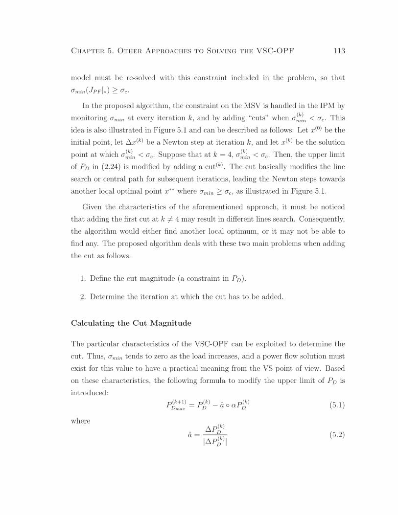
Chapter 5. Other Approaches to Solving the VSC-OPF 113
model must be re-solved with this constraint included in the problem, so that
σmin(JPF |∗) ≥ σc.
In the proposed algorithm, the constraint on the MSV is handled in the IPM by
monitoring σmin at every iteration k, and by adding “cuts” when σ(k)min < σc. This
idea is also illustrated in Figure 5.1 and can be described as follows: Let x(0) be the
initial point, let ∆x(k) be a Newton step at iteration k, and let x(k) be the solution
point at which σ(k)min < σc. Suppose that at k = 4, σ
(k)min < σc. Then, the upper limit
of PD in (2.24) is modified by adding a cut(k). The cut basically modifies the line
search or central path for subsequent iterations, leading the Newton steps towards
another local optimal point x∗∗ where σmin ≥ σc, as illustrated in Figure 5.1.
Given the characteristics of the aforementioned approach, it must be noticed
that adding the first cut at k 6= 4 may result in different lines search. Consequently,
the algorithm would either find another local optimum, or it may not be able to
find any. The proposed algorithm deals with these two main problems when adding
the cut as follows:
1. Define the cut magnitude (a constraint in PD).
2. Determine the iteration at which the cut has to be added.
Calculating the Cut Magnitude
The particular characteristics of the VSC-OPF can be exploited to determine the
cut. Thus, σmin tends to zero as the load increases, and a power flow solution must
exist for this value to have a practical meaning from the VS point of view. Based
on these characteristics, the following formula to modify the upper limit of PD is
introduced:
P(k+1)Dmax
= P(k)D − a ◦ αP
(k)D (5.1)
where
a =∆P
(k)D
|∆P(k)D |
(5.2)
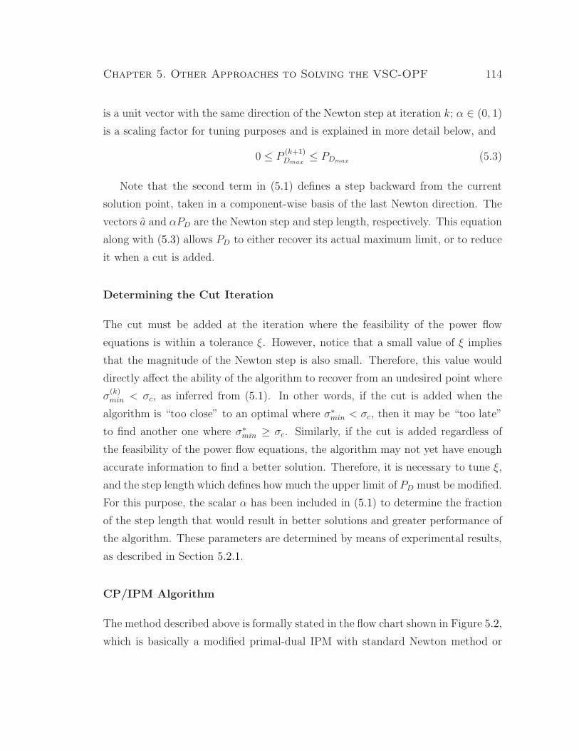
Chapter 5. Other Approaches to Solving the VSC-OPF 114
is a unit vector with the same direction of the Newton step at iteration k; α ∈ (0, 1)
is a scaling factor for tuning purposes and is explained in more detail below, and
0 ≤ P(k+1)Dmax
≤ PDmax (5.3)
Note that the second term in (5.1) defines a step backward from the current
solution point, taken in a component-wise basis of the last Newton direction. The
vectors a and αPD are the Newton step and step length, respectively. This equation
along with (5.3) allows PD to either recover its actual maximum limit, or to reduce
it when a cut is added.
Determining the Cut Iteration
The cut must be added at the iteration where the feasibility of the power flow
equations is within a tolerance ξ. However, notice that a small value of ξ implies
that the magnitude of the Newton step is also small. Therefore, this value would
directly affect the ability of the algorithm to recover from an undesired point where
σ(k)min < σc, as inferred from (5.1). In other words, if the cut is added when the
algorithm is “too close” to an optimal where σ∗min < σc, then it may be “too late”
to find another one where σ∗min ≥ σc. Similarly, if the cut is added regardless of
the feasibility of the power flow equations, the algorithm may not yet have enough
accurate information to find a better solution. Therefore, it is necessary to tune ξ,
and the step length which defines how much the upper limit of PD must be modified.
For this purpose, the scalar α has been included in (5.1) to determine the fraction
of the step length that would result in better solutions and greater performance of
the algorithm. These parameters are determined by means of experimental results,
as described in Section 5.2.1.
CP/IPM Algorithm
The method described above is formally stated in the flow chart shown in Figure 5.2,
which is basically a modified primal-dual IPM with standard Newton method or
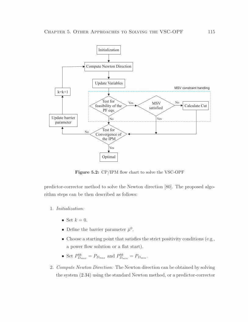
Chapter 5. Other Approaches to Solving the VSC-OPF 115
Initialization
Compute Newton Direction
Update Variables
Calculate Cut
Test forConvergence of
the IPM
MSVsatisfied
Test forfeasibility of the
PF eqs.
Update barrierparameter
Optimal
k=k+1
No
Yes
Yes
Yes
No
No
MSV constraint handling
Figure 5.2: CP/IPM flow chart to solve the VSC-OPF
predictor-corrector method to solve the Newton direction [80]. The proposed algo-
rithm steps can be then described as follows:
1. Initialization:
• Set k = 0.
• Define the barrier parameter µ0.
• Choose a starting point that satisfies the strict positivity conditions (e.g.,
a power flow solution or a flat start).
• Set P bkDmax
= PDmax and P bkDmin
= PDmin.
2. Compute Newton Direction: The Newton direction can be obtained by solving
the system (2.34) using the standard Newton method, or a predictor-corrector

Chapter 5. Other Approaches to Solving the VSC-OPF 116
method.
3. Update Variables: Compute the step length parameters for primal and dual
variables using (2.38)-(2.39), and update the variables using (2.40).
4. Test for Feasibility of the Power Flow Equations: If the feasibility is within
a predetermined tolerance ξ, then start monitoring σmin using a SVD.
• If σ(k)min < σc, i.e., the MSV constraint is not satisfied, then proceed
to calculate the cut as follows: Use equation (5.1), and verify if 0 ≤P
(k+1)Dmax
≤ PDmax . If P(k+1)Dmax
> PDmax , then set P(k+1)Dmax
= P bkDmax
. A similar
process for the lower limit is followed.
• Otherwise, continue the iterative process.
5. Test for Convergence: If the new point satisfies the convergence criteria,
stop. Otherwise, set k = k + 1, update the barrier parameter µk, and return
to Step 1.
Tuning of the Algorithm
As in many iterative solution methods such as the Newton method, determining
the step length parameters is one of the most important issues to ensure a good
performance of the algorithm. Different approaches to calculate these parameters
have been proposed. For instance, separate step lengths for primal and dual vari-
ables are used to update the variables in the IPM [80]; dynamic adjustments of
step sizes and tolerances have been proposed in [100]. One common practice is to
calculate these parameters based on heuristic methods.
In the proposed algorithm, choosing an adequate value for ξ and α is a problem
independent of determining the step length parameters of the Newton direction. It
also requires a heuristic type of method to ensure that the algorithm converges to
a desired solution point in a reasonable number of iterations. Thus, experimental

Chapter 5. Other Approaches to Solving the VSC-OPF 117
results are needed to study how the algorithm performs when the cut is added at
different iterations, in combination with different step sizes.
Let ξ = {NPF, 1 × 10⁻¹, 1 × 10⁻², 1 × 10⁻³, 1 × 10⁻⁴} be a set of threshold
values to test the feasibility of the power flow equations at iteration k. If ξ = NPF
no test is carried out and the cut is added at any iteration where σ(k)min < σc. If
ξ 6= NPF and if σ(k)min < σc, then a cut is added at iteration k. On the other hand,
α ∈ (0, 1) is used to take a fraction of the Newton step at the current iteration. If
α = 0, then P(k+1)Dmax
= P(k)D ; whereas, α = 1 takes a full step backwards in the same
direction of the last Newton step in order to avoid the point P(k)D , as this value
results in a violation of the MSV constraint.
Figures 5.3-5.10 show different optimal solutions for different combinations of
ξ and α, using an IPM with a Newton or predictor-corrector method, initialized
using a flat start or a power flow solution start. The 6-bus test system and the
CIGRE-32 test system presented in Appendix A were used to test the proposed
algorithm. The CP/IPM algorithm was implemented in Matlab.
Figures 5.3(a), 5.3(b), 5.4(a) and 5.4(b) show the MSV of the power flow Jaco-
bian at the optimal solution for various values of α and ξ; the results correspond to
the 6-bus system for σc = 5.0. These figures show that for various (α, ξ) values, the
algorithm satisfies σmin ≥ σc, while it fails for others. One of the most significant
results is that if the cut is added at any iteration where the MSV constraint is
violated (ξ = NPF), a higher value of the MSV is obtained; thus, observe that the
(α, NPF) values provide a solution with a higher MSV than other cases where the
feasibility of the power flow equations is tested at every iteration before adding a
cut. For instance, the combination (1, NPF) generally results in the highest MSV
values, which means that if a full Newton step is taken backwards whenever the
MSV constraint is violated, the algorithm encounters a wider feasible region where
it can find the desired optimal point. From these results, it could be concluded
that the best values are α = 1 and ξ = NPF; thus, let the algorithm add the cut at
any iteration where σ(k)min < σc, and take a full Newton step backward to calculate
P(k+1)Dmax
. However, observe in Figures 5.5(a), 5.5(b), 5.6(a) and 5.6(b), that if such
Chapter 5. Other Approaches to Solving the VSC-OPF 118
criteria are used, the lowest transaction levels (T =∑
PLoi+ PDi
) are obtained,
which yields a lower objective function (SW) value, as shown in Figures 5.7(a),
5.7(b), 5.8(a) and 5.8(b). This is to be expected, since a higher MSV requires a
lower demand levels, since the security margins are higher. Therefore, adding a cut
is equivalent to shedding load from the demand block bids represented by PD to
maintain the required security levels given by the constraint σmin ≥ σc.
Notice that the combinations (0, ξ) represent a cut P(k+1)D = P
(k)D . This results
in the algorithm getting “stuck” trying to avoid the solution point x(k). This can
be observed in Figures 5.9(a), 5.9(b), 5.10(a) and 5.10(b), where it is shown that
the maximum number of iterations (k = 250) is reached. Observe in these figures
that the algorithm performs very well for all ξ, and for all α close to one.
Figures 5.11(a), 5.11(b), 5.12(a) and 5.12(b) show the cuts calculated at every
iteration for different solution methods and starting points. These figures corre-
spond to the case where the cut is added only if the feasibility of the power flow
equations is within ξ = 1 × 10⁻³. Observe that the limits do not change during
the first iterations, thus some cuts are added until the algorithm finds a feasible
point where σ(k)min ≥ σc, and then converges to an optimal point. Notice that (5.3)
holds during the solution process, as required. However, the results in these figures
along with those described above, show that the algorithm is highly dependent on
both the solution method and on the starting point, since (5.1) is different in all
four cases, yielding different optimal solutions. This problem is also observed in
Figure 5.13, which shows σ(k)min using different solution methods and starting points,
as well as the application of the cut for the criteria ξ = NPF or ξ = 1 × 10⁻³.
Notice that the final value of σ(k)min is closer to σc if the cut is applied only if the
feasibility of the power flow equations is within ξ = 1 × 10⁻³. This is the desired
final value of the MSV, since the power dispatch and transaction levels are better
when it is closer to σc.
Figure 5.14 shows the most representative result for the CIGRE-32 test system.
Observe that a similar response of the algorithm for this larger and heavily loaded
system.

Chapter 5. Other Approaches to Solving the VSC-OPF 119
0 0.010.020.030.040.050.060.070.080.090.1 0.2 0.3 0.4 0.5 0.6 0.7 0.8 0.9 1
NPF
0.1
0.01
0.001
0.0001
4.99
4.995
5.005
5.01
5.015
5.02
5.025
5.03
5.035
σc
αξ
σm
in(J
PF
)
(a)
0 0.010.020.030.040.050.060.070.080.090.1 0.2 0.3 0.4 0.5 0.6 0.7 0.8 0.9 1 NPF
0.1
0.01
0.001
0.0001
4.99
4.995
5.005
5.01
5.015
5.02
5.025
5.03
5.035
σc
αξ
σm
in(J
PF
)
(b)
Figure 5.3: MSV of the power flow Jacobian using a Newton method: (a)
flat start; (b) power flow start.

Chapter 5. Other Approaches to Solving the VSC-OPF 120
0 0.01 0.02 0.03 0.04 0.05 0.06 0.07 0.08 0.09 0.1 0.2 0.3 0.4 0.5 0.6 0.7 0.8 0.9 1
NPF
0.1
0.01
0.001
0.0001
4.99
4.995
5.005
5.01
5.015
5.02
5.025
5.03
5.035
σc
αξ
σm
in(J
PF
)
(a)
0 0.01 0.02 0.03 0.04 0.05 0.06 0.07 0.08 0.09 0.1 0.2 0.3 0.4 0.5 0.6 0.7 0.8 0.9 1
NPF
0.1
0.01
0.001
0.0001
4.99
4.995
5.005
5.01
5.015
5.02
5.025
5.03
5.035
σc
αξ
σm
in(J
PF
)
(b)
Figure 5.4: MSV of the power flow Jacobian using a predictor-corrector
method: (a) flat start; (b) power flow start.

Chapter 5. Other Approaches to Solving the VSC-OPF 121
0 0.010.020.030.040.050.060.070.080.090.1 0.2 0.3 0.4 0.5 0.6 0.7 0.8 0.9 1 NPF
0.1
0.01
0.001
0.0001
3
3.05
3.1
3.15
3.2
3.25
αξ
T
(a)
0 0.010.020.030.040.050.060.070.080.090.1 0.2 0.3 0.4 0.5 0.6 0.7 0.8 0.9 1 NPF
0.1
0.01
0.001
0.0001
2.95
3
3.05
3.1
3.15
3.2
3.25
αξ
T
(b)
Figure 5.5: Total transaction level using a Newton method: (a) flat start;
(b) power flow start.

Chapter 5. Other Approaches to Solving the VSC-OPF 122
0 0.010.020.030.040.050.060.070.080.090.1 0.2 0.3 0.4 0.5 0.6 0.7 0.8 0.9 1 NPF
0.1
0.01
0.001
0.0001
2.8
2.85
2.9
2.95
3
3.05
3.1
3.15
3.2
3.25
3.3
αξ
T
(a)
0 0.010.020.030.040.050.060.070.080.090.1 0.2 0.3 0.4 0.5 0.6 0.7 0.8 0.9 1 NPF
0.1
0.01
0.001
0.0001
2.95
3
3.05
3.1
3.15
3.2
3.25
αξ
T
(b)
Figure 5.6: Total transaction level using a predictor-corrector method: (a)
flat start; (b) power flow start.

Chapter 5. Other Approaches to Solving the VSC-OPF 123
0 0.010.020.030.040.050.060.070.080.090.1 0.2 0.3 0.4 0.5 0.6 0.7 0.8 0.9 1 NPF
0.1
0.01
0.001
0.0001
0.8
0.85
0.9
0.95
1
1.05
1.1
1.15
1.2
1.25
αξ
SW
(a)
0 0.010.020.030.040.050.060.070.080.090.1 0.2 0.3 0.4 0.5 0.6 0.7 0.8 0.9 1 NPF
0.1
0.01
0.001
0.0001
0.7
0.8
0.9
1
1.1
1.2
1.3
1.4
αξ
SW
(b)
Figure 5.7: Objective function using a Newton method: (a) flat start; (b)
power flow start.
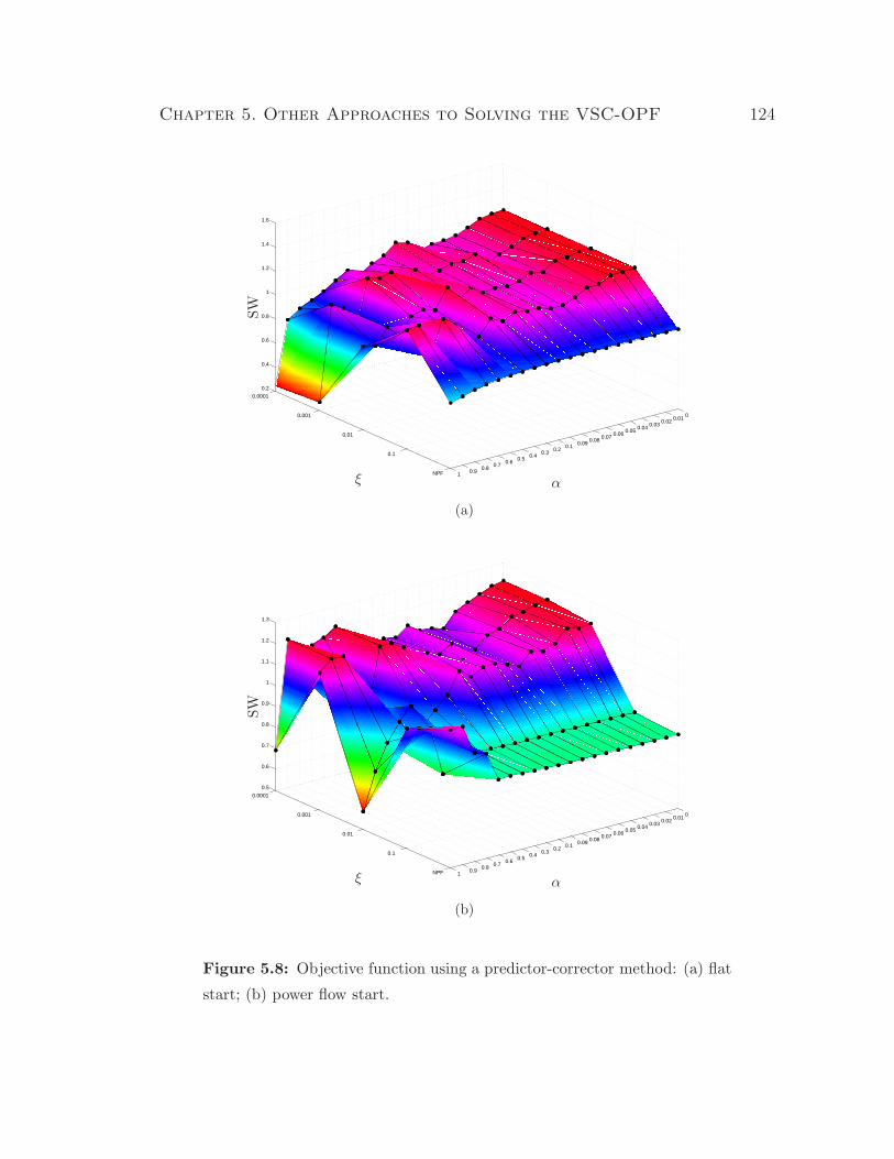
Chapter 5. Other Approaches to Solving the VSC-OPF 124
0 0.010.020.030.040.050.060.070.080.090.1 0.2 0.3 0.4 0.5 0.6 0.7 0.8 0.9 1 NPF
0.1
0.01
0.001
0.0001
0.2
0.4
0.6
0.8
1
1.2
1.4
1.6
αξ
SW
(a)
0 0.010.020.030.040.050.060.070.080.090.1 0.2 0.3 0.4 0.5 0.6 0.7 0.8 0.9 1 NPF
0.1
0.01
0.001
0.0001
0.5
0.6
0.7
0.8
0.9
1
1.1
1.2
1.3
αξ
SW
(b)
Figure 5.8: Objective function using a predictor-corrector method: (a) flat
start; (b) power flow start.
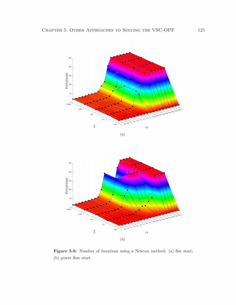
Chapter 5. Other Approaches to Solving the VSC-OPF 125
0 0.010.020.030.040.050.060.070.080.090.1 0.2 0.3 0.4 0.5 0.6 0.7 0.8 0.9 1 NPF
0.1
0.01
0.001
0.0001
0
50
100
150
200
250
αξ
Iter
ations
(a)
0 0.010.020.030.040.050.060.070.080.090.1 0.2 0.3 0.4 0.5 0.6 0.7 0.8 0.9 1 NPF
0.1
0.01
0.001
0.0001
0
50
100
150
200
250
αξ
Iter
ations
(b)
Figure 5.9: Number of iterations using a Newton method: (a) flat start;
(b) power flow start.

Chapter 5. Other Approaches to Solving the VSC-OPF 126
0 0.010.020.030.040.050.060.070.080.090.1 0.2 0.3 0.4 0.5 0.6 0.7 0.8 0.9 1 NPF
0.1
0.01
0.001
0.0001
0
50
100
150
200
250
αξ
Iter
ations
(a)
0 0.010.020.030.040.050.060.070.080.090.1 0.2 0.3 0.4 0.5 0.6 0.7 0.8 0.9 1 NPF
0.1
0.01
0.001
0.0001
0
50
100
150
200
250
αξ
Iter
ations
(b)
Figure 5.10: Number of iterations using a predictor-corrector method: (a)
flat start; (b) power flow start.

Chapter 5. Other Approaches to Solving the VSC-OPF 127
2 4 6 8 10 12 14 16 18 20 220
0.05
0.1
0.15
0.2
0.25
PD1max(k)
PD2max(k)
PD3max(k)
PD1max
PD2max
PD3max
k
PD
ma
x[p
.u.]
(a)
0 5 10 15 200
0.05
0.1
0.15
0.2
0.25
PD1max(k)
PD2max(k)
PD3max(k)
PD1max
PD2max
PD3max
k
PD
ma
x[p
.u.]
(b)
Figure 5.11: Cuts at every iteration using a Newton method: (a) flat start;
(b) power flow start.
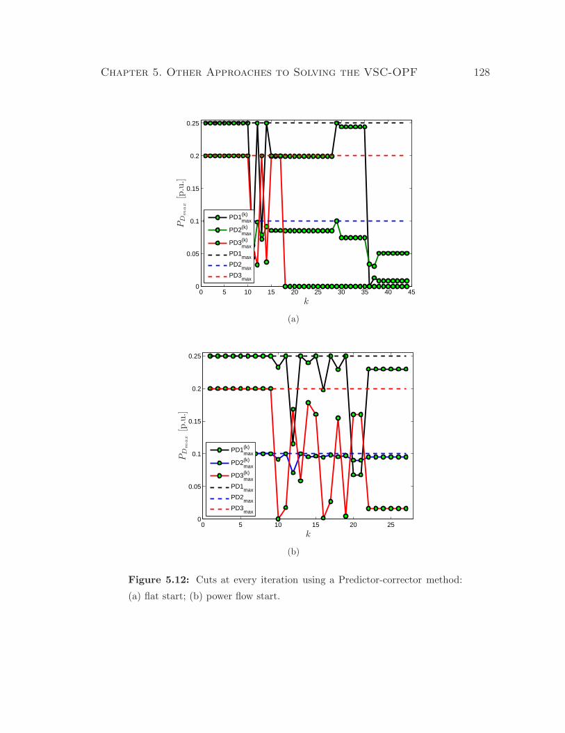
Chapter 5. Other Approaches to Solving the VSC-OPF 128
0 5 10 15 20 25 30 35 40 450
0.05
0.1
0.15
0.2
0.25
PD1max(k)
PD2max(k)
PD3max(k)
PD1max
PD2max
PD3max
k
PD
ma
x[p
.u.]
(a)
0 5 10 15 20 250
0.05
0.1
0.15
0.2
0.25
PD1max(k)
PD2max(k)
PD3max(k)
PD1max
PD2max
PD3max
k
PD
ma
x[p
.u.]
(b)
Figure 5.12: Cuts at every iteration using a Predictor-corrector method:
(a) flat start; (b) power flow start.
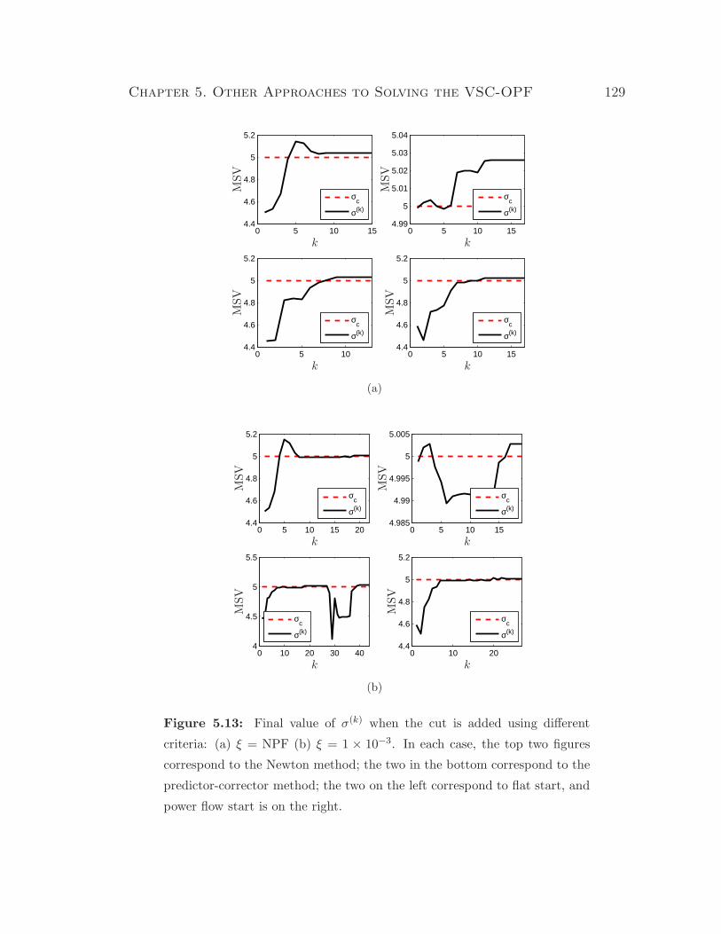
Chapter 5. Other Approaches to Solving the VSC-OPF 129
0 5 10 154.4
4.6
4.8
5
5.2
σc
σ(k)
0 5 10 154.99
5
5.01
5.02
5.03
5.04
σc
σ(k)
0 5 104.4
4.6
4.8
5
5.2
σc
σ(k)
0 5 10 154.4
4.6
4.8
5
5.2
σc
σ(k)
kk
kk
MSV
MSV
MSV
MSV
(a)
0 5 10 15 204.4
4.6
4.8
5
5.2
σc
σ(k)
0 5 10 154.985
4.99
4.995
5
5.005
σc
σ(k)
0 10 20 30 404
4.5
5
5.5
σc
σ(k)
0 10 204.4
4.6
4.8
5
5.2
σc
σ(k)
kk
kk
MSV
MSV
MSV
MSV
(b)
Figure 5.13: Final value of σ(k) when the cut is added using different
criteria: (a) ξ = NPF (b) ξ = 1 × 10⁻³. In each case, the top two figures
correspond to the Newton method; the two in the bottom correspond to the
predictor-corrector method; the two on the left correspond to flat start, and
power flow start is on the right.

Chapter 5. Other Approaches to Solving the VSC-OPF 130
0.010.02
0.030.04
0.060.07
0.080.2
0.3 0.4
0.6 0.7
1
NPF
0.1
0.01
0.001
0.0001
0.795
0.805
0.81
0.815
σc
αξ
σm
in(J
PF)
Figure 5.14: MSV of the power flow Jacobian using a predictor-corrector
method with a power flow start for the CIGRE-32 test system.
After several tests, it was concluded that the best values in general are α = 1
and ξ = 1 × 10⁻³. It was also observed that the algorithm performs well using
either the Newton method or the predictor-corrector method; however, the later
usually required less iterations.
5.2.2 Numerical Results
Having studied and tuned the algorithm, a comparison between the CP/IPM al-
gorithm and the proposed method presented in Chapter 4 to solve the VSC-OPF
model (2.24) is presented in this section. These methods are applied to the same
6-bus test system, and the CIGRE-32 system. The σc value used in the MSV
constraint for each system is σc = 5.0 and σc = 0.8, respectively. The CP/IPM al-
gorithm was solved using the Newton method with a power flow start, ξ = 1×10⁻³
and α = 1.
The results presented in Table 5.1, corresponding to the 6-bus system, show
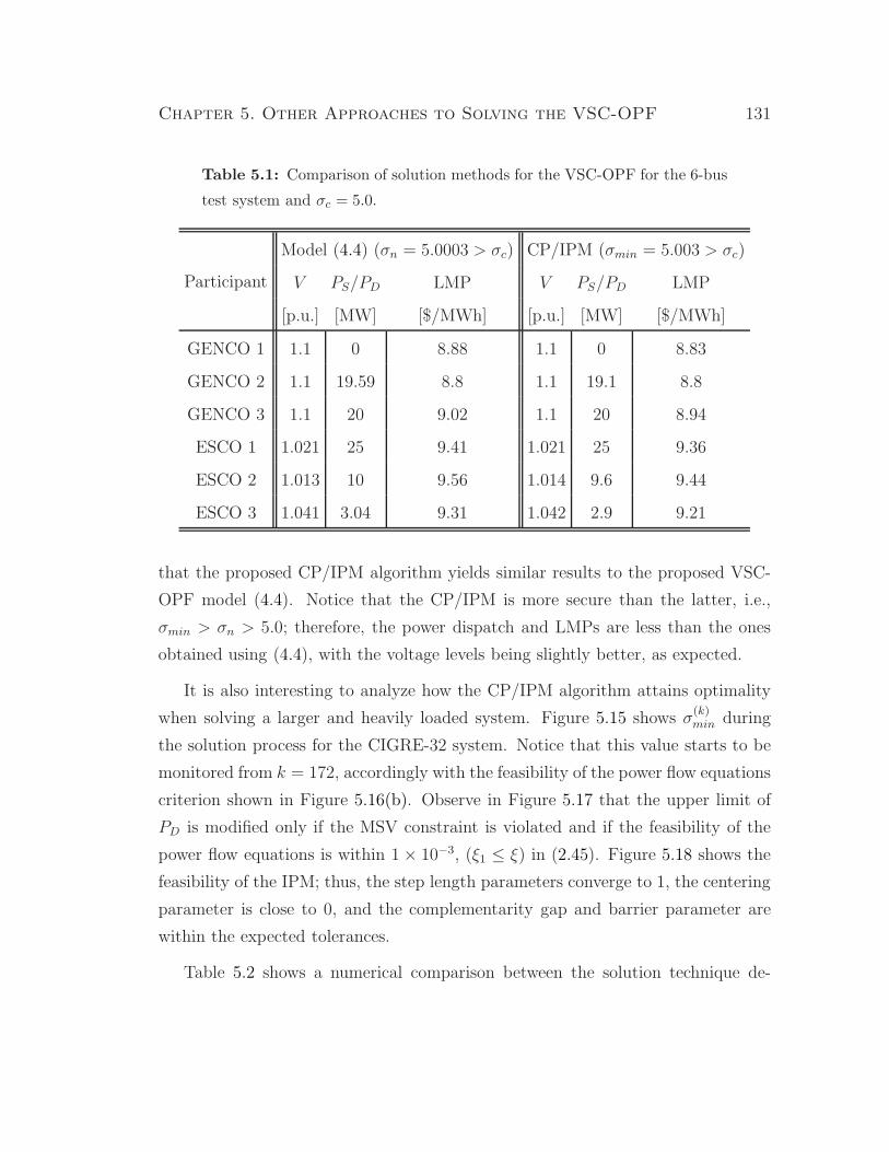
Chapter 5. Other Approaches to Solving the VSC-OPF 131
Table 5.1: Comparison of solution methods for the VSC-OPF for the 6-bus
test system and σc = 5.0.
Participant
Model (4.4) (σn = 5.0003 > σc) CP/IPM (σmin = 5.003 > σc)
V PS/PD LMP V PS/PD LMP
[p.u.] [MW] [$/MWh] [p.u.] [MW] [$/MWh]
GENCO 1 1.1 0 8.88 1.1 0 8.83
GENCO 2 1.1 19.59 8.8 1.1 19.1 8.8
GENCO 3 1.1 20 9.02 1.1 20 8.94
ESCO 1 1.021 25 9.41 1.021 25 9.36
ESCO 2 1.013 10 9.56 1.014 9.6 9.44
ESCO 3 1.041 3.04 9.31 1.042 2.9 9.21
that the proposed CP/IPM algorithm yields similar results to the proposed VSC-
OPF model (4.4). Notice that the CP/IPM is more secure than the latter, i.e.,
σmin > σn > 5.0; therefore, the power dispatch and LMPs are less than the ones
obtained using (4.4), with the voltage levels being slightly better, as expected.
It is also interesting to analyze how the CP/IPM algorithm attains optimality
when solving a larger and heavily loaded system. Figure 5.15 shows σ(k)min during
the solution process for the CIGRE-32 system. Notice that this value starts to be
monitored from k = 172, accordingly with the feasibility of the power flow equations
criterion shown in Figure 5.16(b). Observe in Figure 5.17 that the upper limit of
PD is modified only if the MSV constraint is violated and if the feasibility of the
power flow equations is within 1× 10⁻³, (ξ1 ≤ ξ) in (2.45). Figure 5.18 shows the
feasibility of the IPM; thus, the step length parameters converge to 1, the centering
parameter is close to 0, and the complementarity gap and barrier parameter are
within the expected tolerances.
Table 5.2 shows a numerical comparison between the solution technique de-

Chapter 5. Other Approaches to Solving the VSC-OPF 132
0 50 100 150 200 250 300 3500.72
0.74
0.76
0.78
0.8
0.82
0.84
0.86
σmin(k)
σc
Cuts start to apply at k = 172
k
MSV
Figure 5.15: MSV at every iteration in the CP/IPM when solving the
CIGRE-32 system.
scribed in Chapter 4 and the proposed CP/IPM approach. Notice that the small
difference between the σmin values obtained from these two techniques, i.e., 0.00409,
has a significant effect on the power dispatch and LMPs at some buses. This is
to be expected, since a big increase in system demand may result in a very small
change in the MSV; however, this difference can be also attributed to the fact that
these methods just converge to different local optimal. Finally, these results show
that the two proposed methods can successfully solve the VSC-OPF model (2.24).
Nevertheless, in general, the proposed model (4.4) and its solution technique is
better than the CP/IPM algorithm, because:
• The CP/IPM method depends on the starting point and on the solution
technique, yielding different solutions, whereas (4.4) does not.
• The CP/IPM method requires elastic demand bids, which limits its appli-
cation to other OPF problems, since in most electricity markets, demand is

Chapter 5. Other Approaches to Solving the VSC-OPF 133
0 50 100 150 200 250 300 35010
−14
10−12
10−10
10−8
10−6
10−4
10−2
100
k
ξ 4
(a)
0 50 100 150 200 250 300 35010
−8
10−6
10−4
10−2
100
102
ξ
k
ξ 1
(b)
Figure 5.16: Feasibility of (a) the objective function and (b) the power flow
equations (equality constraints) in the CP/IPM when solving the CIGRE-32
system.

Chapter 5. Other Approaches to Solving the VSC-OPF 134
0 50 100 150 200 250 300 350−5
0
5
10
15
20
PD1max(k)
PD2max(k)
PD3max(k)
PD1max
PD2max
PD3max
Cuts start to apply at k=172
k
PD
ma
x[M
W]
Figure 5.17: The box encloses the iterations at which some cuts are added
in the CP/IPM when solving CIGRE-32 system.
inelastic. This is not the case for (4.4), which works for any type of load
demand.
Table 5.2: Comparison of the proposed solution methods for the VSC-OPF
using the CIGRE-32 test system, for σc = 0.8.
Bus
Model (4.4) (σn = σc = 0.8) CP/IPM (σmin = 0.80409 > σc)
V PS PD LMP V PS PD LMP
[p.u.] [MW] [MW] [$/MWh] [p.u.] [MW] [MW] [$/MWh]
4072 0.972 0 845.224 10.000 0.985 0 856.5 9.950
4071 0.964 0 0 9.499 0.972 0 0 9.360
4011 1.016 227.548 0 9.000 1.017 0 0 8.724
4012 1.009 600.6 0 8.734 1.009 573.06 0 8.500
Continued on next page

Chapter 5. Other Approaches to Solving the VSC-OPF 135
Table 5.2 – continued from previous page
Bus
Model (4.4) (σn = σc = 0.8) CP/IPM (σmin = 0.80409 > σc)
V PS PD LMP V PS PD LMP
[p.u.] [MW] [MW] [$/MWh] [p.u.] [MW] [MW] [$/MWh]
4021 1.100 0 0 6.517 1.100 0 0 6.861
4031 1.001 19.333 0 7.500 0.994 256.39 0 7.500
4042 0.978 658 0 7.289 0.971 0 0 6.761
4041 1.018 282 0 7.888 0.992 282 0 7.421
4062 1.094 564 0 6.388 1.009 564 0 6.171
4063 1.098 884.778 0 5.500 1.006 878.84 0 5.500
4051 1.009 658 0 8.257 0.979 658 0 7.215
4047 1.002 769.6 0 7.841 0.963 769.6 0 6.983
2032 0.968 728.277 200 4.000 0.977 694.06 200 4.000
1013 1.011 543.2 100 7.869 1.011 543.2 99.995 7.582
1012 0.900 0 300 8.717 0.900 0 300 8.473
1014 1.031 0 0 7.962 1.031 0 0 7.692
1022 0.920 0 280 8.202 0.900 0 280 8.118
1021 1.100 0 0 6.841 1.057 0 0 6.819
1043 0.964 0 0 9.677 0.932 0 17.088 8.363
1042 1.100 0 0 8.302 1.100 0 0 7.143
4022 1.004 0 0 8.200 0.996 0 0 8.104
4032 1.035 0 0 6.960 1.029 0 0 7.072
4043 0.946 0 0 8.384 0.947 0 0 7.077
4044 0.969 0 0 8.264 0.955 0 0 7.203
Continued on next page
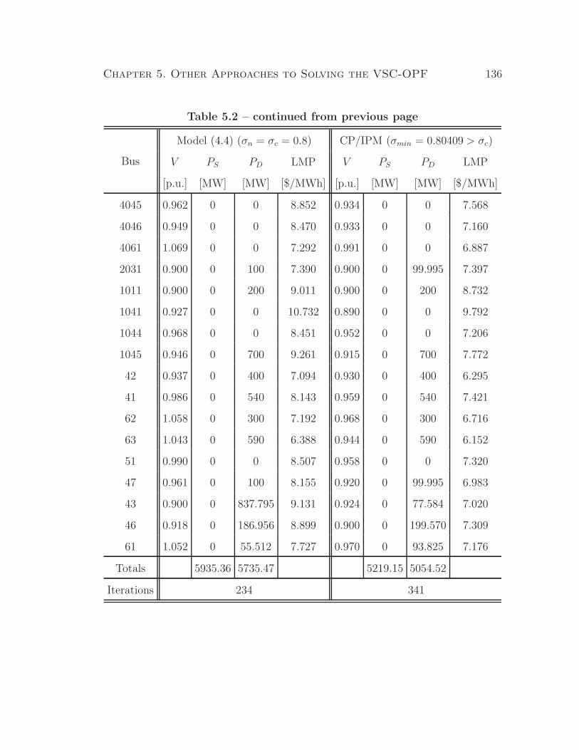
Chapter 5. Other Approaches to Solving the VSC-OPF 136
Table 5.2 – continued from previous page
Bus
Model (4.4) (σn = σc = 0.8) CP/IPM (σmin = 0.80409 > σc)
V PS PD LMP V PS PD LMP
[p.u.] [MW] [MW] [$/MWh] [p.u.] [MW] [MW] [$/MWh]
4045 0.962 0 0 8.852 0.934 0 0 7.568
4046 0.949 0 0 8.470 0.933 0 0 7.160
4061 1.069 0 0 7.292 0.991 0 0 6.887
2031 0.900 0 100 7.390 0.900 0 99.995 7.397
1011 0.900 0 200 9.011 0.900 0 200 8.732
1041 0.927 0 0 10.732 0.890 0 0 9.792
1044 0.968 0 0 8.451 0.952 0 0 7.206
1045 0.946 0 700 9.261 0.915 0 700 7.772
42 0.937 0 400 7.094 0.930 0 400 6.295
41 0.986 0 540 8.143 0.959 0 540 7.421
62 1.058 0 300 7.192 0.968 0 300 6.716
63 1.043 0 590 6.388 0.944 0 590 6.152
51 0.990 0 0 8.507 0.958 0 0 7.320
47 0.961 0 100 8.155 0.920 0 99.995 6.983
43 0.900 0 837.795 9.131 0.924 0 77.584 7.020
46 0.918 0 186.956 8.899 0.900 0 199.570 7.309
61 1.052 0 55.512 7.727 0.970 0 93.825 7.176
Totals 5935.36 5735.47 5219.15 5054.52
Iterations 234 341
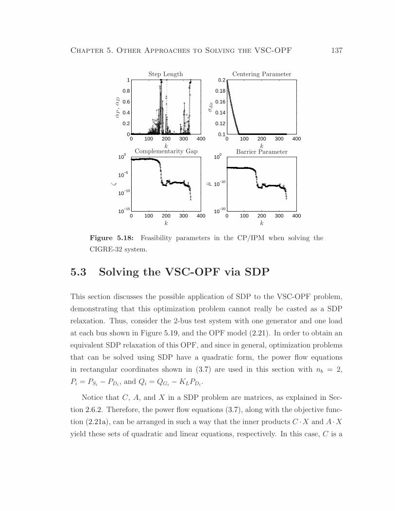
Chapter 5. Other Approaches to Solving the VSC-OPF 137
0 100 200 300 4000
0.2
0.4
0.6
0.8
1
0 100 200 300 4000.1
0.12
0.14
0.16
0.18
0.2
0 100 200 300 40010
−15
10−10
10−5
100
0 100 200 300 40010
−20
10−10
100
kk
kk
αP
,α
D
σdir
ζ µ
Step Length Centering Parameter
Complementarity Gap Barrier Parameter
Figure 5.18: Feasibility parameters in the CP/IPM when solving the
CIGRE-32 system.
5.3 Solving the VSC-OPF via SDP
This section discusses the possible application of SDP to the VSC-OPF problem,
demonstrating that this optimization problem cannot really be casted as a SDP
relaxation. Thus, consider the 2-bus test system with one generator and one load
at each bus shown in Figure 5.19, and the OPF model (2.21). In order to obtain an
equivalent SDP relaxation of this OPF, and since in general, optimization problems
that can be solved using SDP have a quadratic form, the power flow equations
in rectangular coordinates shown in (3.7) are used in this section with nb = 2,
Pi = PSi− PDi
, and Qi = QGi−KLPDi
.
Notice that C, A, and X in a SDP problem are matrices, as explained in Sec-
tion 2.6.2. Therefore, the power flow equations (3.7), along with the objective func-
tion (2.21a), can be arranged in such a way that the inner products C ·X and A ·Xyield these sets of quadratic and linear equations, respectively. In this case, C is a

Chapter 5. Other Approaches to Solving the VSC-OPF 138
P +jQS1 S1
G+jB
P +jQS2 S2
P +jQD2 D2P +jQD1 D1
Figure 5.19: 2-bus system
matrix containing the coefficients CD and CS of the objective function; A is a matrix
containing all the constraints coefficients; and X is a matrix containing all the vari-
ables. For example, the objective function in (2.49) for x = [er1fr1
er2fr2
PS1PD1
1]T
yields:
X = xxT =
e2r1
er1fr1
er1er2
er1fr2
er1PS1
er1PD1
er1
er1fr1
f 2r1
er2fr1
fr1fr2
fr1PS1
fr1PD1
fr1
er1er2
er2fr1
e2r2
er2fr2
er2PS1
er2PD1
er2
er1fr2
fr1fr2
er2fr2
f 2r2
fr2PS1
fr2PD1
fr2
er1PS1
fr1PS1
er2PS1
fr2PS1
P 2S1
PS1PD1
PS1
er1PD1
fr1PD1
er2PD1
fr2PD1
PD1PS1
P 2D1
PD1
er1fr1
er2fr2
PS1PD1
1
(5.4)
or
X =
er1er1
fr1er1
er2er1
fr2er1
PS1er1
PD1er1
er1fr1
fr1er2
fr1fr1
fr2fr1
PS1fr1
PD1fr1
er1er2
er2fr1
er2er2
fr2er2
PS1er2
PD1er2
er1fr2
fr1fr2
er2fr2
fr2fr2
PS1fr2
PD1fr2
er1PS1
fr1PS1
er2PS1
fr2PS1
PS1PS1
PD1PS1
er1PD1
fr1PD1
er2PD1
fr2PD1
PD1PS1
PD1PD1
er1fr1
er2fr2
PS1PD1
1
(5.5)
where er1= (er1
)2; fr1= (fr1
)2; er2= (er2
)2; fr2= (fr2
)2; PS1= (PS1
)2, and PD1=
(PD1)2 are considered variables in the SDP solution process, and the coefficient
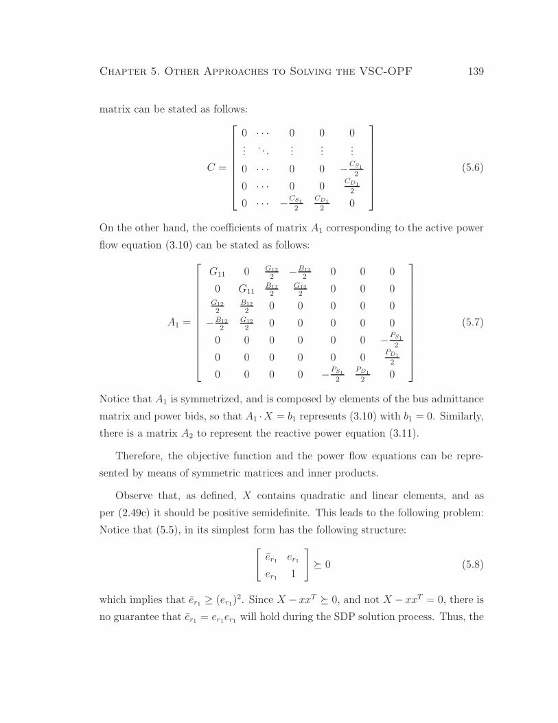
Chapter 5. Other Approaches to Solving the VSC-OPF 139
matrix can be stated as follows:
C =
0 · · · 0 0 0...
. . ....
......
0 · · · 0 0 −CS1
2
0 · · · 0 0CD1
2
0 · · · −CS1
2
CD1
20
(5.6)
On the other hand, the coefficients of matrix A1 corresponding to the active power
flow equation (3.10) can be stated as follows:
A1 =
G11 0 G12
2−B12
20 0 0
0 G11B12
2G12
20 0 0
G12
2B12
20 0 0 0 0
−B12
2G12
20 0 0 0 0
0 0 0 0 0 0 −PS1
2
0 0 0 0 0 0PD1
2
0 0 0 0 −PS1
2
PD1
20
(5.7)
Notice that A1 is symmetrized, and is composed by elements of the bus admittance
matrix and power bids, so that A1 ·X = b1 represents (3.10) with b1 = 0. Similarly,
there is a matrix A2 to represent the reactive power equation (3.11).
Therefore, the objective function and the power flow equations can be repre-
sented by means of symmetric matrices and inner products.
Observe that, as defined, X contains quadratic and linear elements, and as
per (2.49c) it should be positive semidefinite. This leads to the following problem:
Notice that (5.5), in its simplest form has the following structure:
[er1
er1
er11
]� 0 (5.8)
which implies that er1≥ (er1
)2. Since X − xxT � 0, and not X − xxT = 0, there is
no guarantee that er1= er1
er1will hold during the SDP solution process. Thus, the
Chapter 5. Other Approaches to Solving the VSC-OPF 140
variable matrix (5.5) does not accurately represent the variables of the problem. In
conclusion, the nonlinear OPF cannot really be cast as an SDP problem.
It should be mentioned that SDP has been successfully applied to 0/1 problems
such as power dispatch [10] and hydrothermal coordination [9], where nonconvex
integer-value constraints are replaced by convex quadratic constraints.
5.4 Summary
Two alternative methods to solving the MSV-based VSC-OPF model are studied
in this chapter. In the first method, a CP technique is used to handle the VS
constraint at every iteration of the primal-dual IPM method. The handling of the
VS constraint consist of modifying the upper limit of the demand block bids (adding
a cut) when the MSV at a particular iteration is less than a predetermined value.
By doing this, the load power dispatch is reduced until the MSV constraint holds,
since it is well known that the MSV of the power flow Jacobian decreases when the
load increases.
The results obtained for two test systems show that the proposed algorithm
successfully solves the VSC-OPF, and that is somewhat comparable with respect
to the proposed method in Chapter 4. However, its dependency on both the solution
method and on the starting point, as well as the need for an elastic demand, limit
the practical application of the algorithm.
The possible use of SDP is also studied, since the inherent constraint on the
positivity of the matrix variable in SDP could be related to the required nonsin-
gularity of the power flow Jacobian in the MSV-based VSC-OPF. It is shown that
the OPF in rectangular form with social welfare as the objective function can be
represented with the inner product of two matrices, as needed in SDP. However,
it is also demonstrated that this OPF cannot really be casted as a SDP relaxation
problem.

Chapter 6
Conclusions
6.1 Summary
This thesis concentrates on the analysis of an optimization-based method for VS
studies, and on the development of solution techniques for VSC-OPF-based auction
models. A detailed theoretical study of an optimization method to determine the
maximum point of loadability at which a power system experiences a voltage col-
lapse is presented. A novel and practical method to solve a VSC-OPF model which
represents VS through the use of the MSV of the power flow Jacobian is proposed.
Furthermore, a modified primal-dual IPM to solve a VSC-OPF model using CP is
proposed, and SDP is also investigated as a possible solution method.
The following summarizes the main content and conclusions of this thesis:
• Chapter 3 studies in detail the OPF-DM. It is analytically shown that the
optimal point of this model corresponds to a SNB or LISB point. This is
accomplished by demonstrating that the KKT optimality conditions at the
solution of this model yield the same transversality conditions that charac-
terize these bifurcations in nonlinear theory. Numerical examples are also
presented to show the numerical equivalence between the OPF-DM and the
141
Chapter 6. Conclusions 142
CPF technique. The results show that the optimization model is a very flex-
ible tool to study these bifurcations, as current mathematical programming
languages and solvers allow one to efficiently solve this problem. Furthermore,
this model has been extended to optimize other system parameters so that
the loadability of the system is maximized.
• In Chapter 4, a novel and practical method to solve a VSC-OPF which in-
corporates a VS constraint through the use of the SVD of the power flow
Jacobian is proposed. The method consists of iterating to update the SVD
of the power flow Jacobian at an optimal power flow solution, until a prede-
termined MSV is satisfied. A comparison between the proposed VSC-OPF
and a typical SC-OPF is presented to highlight the advantages of the VSC-
OPF model. The proposed VSC-OPF model is applied to small and large
test systems of up to 1211 buses to study its performance and to demonstrate
its robustness and practical application in realistic systems. The results from
this research yield the following conclusions:
– The main problem in the formulation of a MSV-based VS constraint
is to find an explicit function constraint that can be readily written in
terms of the VSC-OPF optimization variables, since the MSV constraint
in the originally proposed model is an implicit function.
– In the proposed VSC-OPF model, the VS constraint (uTnJPFwn ≥ σc)
becomes explicit. This constraint and corresponding solution technique
are shown to computationally outperform the previously proposed MSV-
based VSC-OPF model.
– The main advantages of the proposed model and solution technique are
that it is easy to implement using mathematical programming languages,
and that there is no need for approximations of the MSV constraint
during the solution process. These advantages result in a more robust
and practical model.

Chapter 6. Conclusions 143
– The proposed VSC-OPF model is shown to better represent power sys-
tem security, resulting in better system and market conditions with re-
spect to SC-OPF models.
– The main disadvantage of the proposed method is that it requires an
iterative solution process, where appropriate parameters (un, wn) are
calculated at each iteration. However, experience with different test
systems show that the method converges in less than three iterations
regardless of the system size.
• In Chapter 5, two alternative techniques to solve the VSC-OPF are proposed.
A CP technique to handle the MSV constraint at every iteration of the primal-
dual IPM is first proposed to solve the MSV-based VSC-OPF. The developed
CP/IPM algorithm is based on a basic concept used in mixed-integer linear
optimization, i.e., adding linear constraints (cuts) until the solution holds.
In the proposed CP/IPM algorithm the MSV of the power flow Jacobian
is monitored at every iteration using a SVD. Then, a cut is added at this
iteration if the MSV is less than a predetermined value. The second method
tries to formulate the VSC-OPF as an SDP relaxation, so that the positiveness
of the eigenvalues of the matrix variable can be related to the MSV constraint.
The following conclusions are derived from this investigation:
– Different optimal solutions are obtained depending upon the initial point
and solution method for the Newton direction.
– The algorithm achieves the desired objective by having to tradeoff be-
tween a Newton or predictor-corrector method and flat start or a power
flow start. These trade-offs make it less practical than previously pro-
posed methods.
– It is concluded that the algorithm, in general, has a good performance
using a Newton method with a power flow start.
– The VSC-OPF model cannot be cast as an SDP problem, because the

Chapter 6. Conclusions 144
relaxation of the matrix variables cannot be used to properly formulate
the quadratic terms of the power flow equations in rectangular form.
6.2 Contributions
The main contributions of this thesis to the field of power engineering are:
1. A complete theoretical background that supports the use of the OPF-DM
to determine the maximum point of loadability of a power system has been
developed. This is accomplished by formally demonstrating that the KKT
optimality conditions at the solution of the OPF-DM yield the transversality
conditions for SNBs and LIBs in bifurcation theory.
2. Two methods to solve a MSV-based VSC-OPF model are proposed.
• The first method is a novel and practical VSC-OPF model, where the
implicit function used in a previously proposed model to represent VS
is replaced with an explicit constraint easier to solve and implement,
resulting in a more robust and practical model.
• The second method is a modified primal-dual IPM which makes use of
a CP technique to handle the MSV constraint of the VSC-OPF. The
CP/IPM is different from traditional IPM schemes, and is specially de-
veloped to solve this particular VSC-OPF model.
3. It is analytically shown that the VSC-OPF cannot be cast as an SDP relax-
ation problem.
The main contents of this thesis has been accepted for publication or is under review
for publication in IEEE journals [101,102], and a conference paper has been already
accepted for presentation and publication [103].

Chapter 6. Conclusions 145
6.3 Future Work
Further research may be carried out to address the following issues:
• The use of other VSIs in the VSC-OPF should be studied.
• Other optimization methods to solve the proposed VSC-OPF model should
be studied, e.g., sequential linear programming.
• Multiperiod OPF models are widely used in power system planning and gener-
ation scheduling, among other applications. However, these models are based
on linear OPFs which do not include voltage or reactive power variables;
therefore, these models do not include voltage security constraints. Hence,
developing a linear VSC-OPF would be of great interest.
• The main disadvantage of the proposed CP/IPM algorithm is the dependence
on the initial point and solution method for the Newton direction. Therefore,
a sensitivity-based approach to calculate the cuts could alleviate this problem.

Appendix A
Test Systems
A.1 6-bus Test System
Figure A.1 shows the 6-bus test system, which has been used by many authors to
carry out different studies (e.g., [32,36]) and is also used in this thesis. This system
consists of 6 buses, 3 generators, and 11 transmission lines.
Table A.1 show the supply and demand bids for generators and load demands
respectively, whereas Table A.2 shows the transmission line parameters. Transmis-
sion line limits were computed off-line using a CPF technique, using the generation
and load bids as power directions. Bus voltage minimum and maximum limits
are considered to be 0.9 p.u. and 1.1 p.u. respectively. The data was obtained
from [74].
146

Appendix A. Test Systems 147
Bus 1GENCO 1
Bus 2GENCO 2
Bus 5ESCO 2
Bus 4ESCO 1
Bus 6ESCO 3
Bus 3GENCO 3
Figure A.1: 6-bus test system.
Table A.1: GENCOs and ESCOs bidding data for the 6-bus test system
ParticipantCS/CD PSmax PDmax PLo QLo PGo QGmin/max
($/MWh) (MW) (MW) (MW) (Mvar) (MW) (MVar)
GENCO 1 9.7 20 0 0 0 90 ± 150
GENCO 2 8.8 25 0 0 0 140 ± 150
GENCO 3 7.0 20 0 0 0 60 ± 150
ESCO 1 12.0 0 25 90 60 0 0
ESCO 2 10.5 0 10 100 70 0 0
ESCO 3 9.5 0 20 90 60 0 0
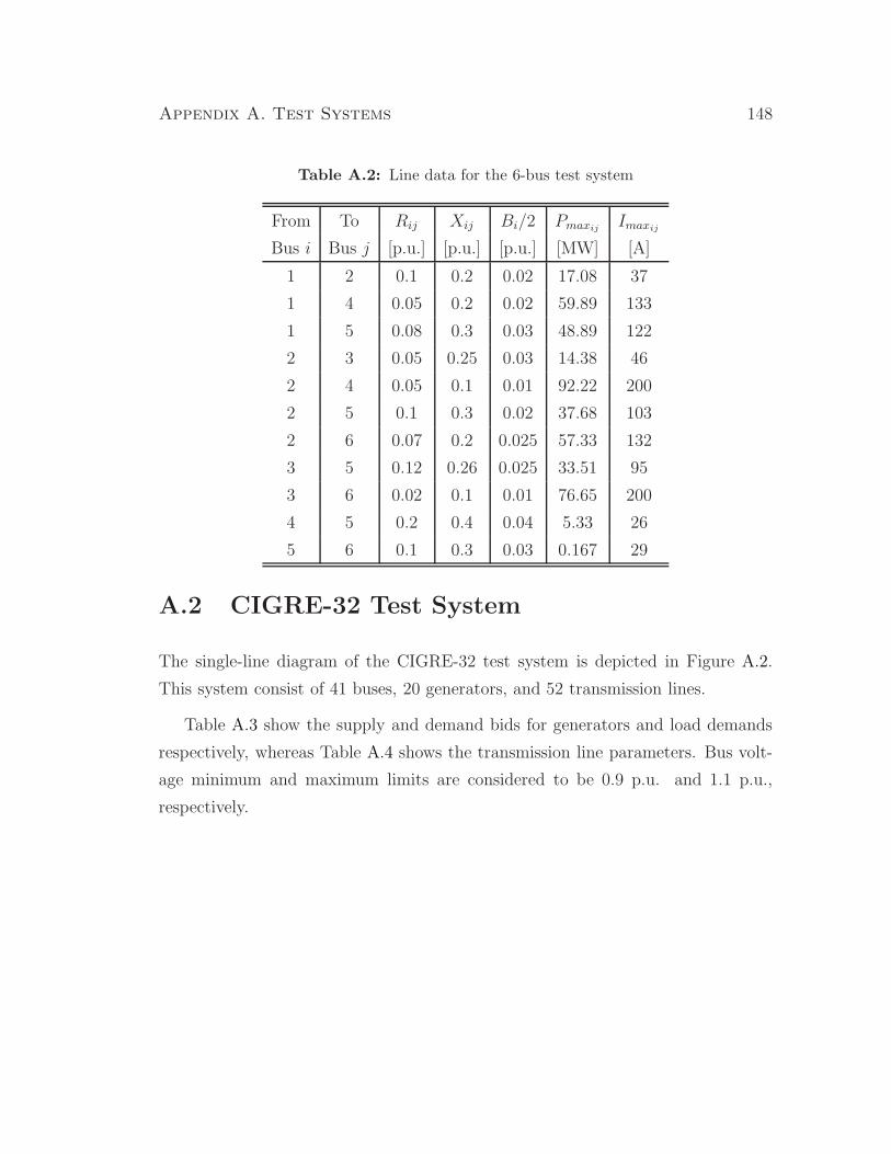
Appendix A. Test Systems 148
Table A.2: Line data for the 6-bus test system
From To Rij Xij Bi/2 PmaxijImaxij
Bus i Bus j [p.u.] [p.u.] [p.u.] [MW] [A]
1 2 0.1 0.2 0.02 17.08 37
1 4 0.05 0.2 0.02 59.89 133
1 5 0.08 0.3 0.03 48.89 122
2 3 0.05 0.25 0.03 14.38 46
2 4 0.05 0.1 0.01 92.22 200
2 5 0.1 0.3 0.02 37.68 103
2 6 0.07 0.2 0.025 57.33 132
3 5 0.12 0.26 0.025 33.51 95
3 6 0.02 0.1 0.01 76.65 200
4 5 0.2 0.4 0.04 5.33 26
5 6 0.1 0.3 0.03 0.167 29
A.2 CIGRE-32 Test System
The single-line diagram of the CIGRE-32 test system is depicted in Figure A.2.
This system consist of 41 buses, 20 generators, and 52 transmission lines.
Table A.3 show the supply and demand bids for generators and load demands
respectively, whereas Table A.4 shows the transmission line parameters. Bus volt-
age minimum and maximum limits are considered to be 0.9 p.u. and 1.1 p.u.,
respectively.

Appendix A. Test Systems 149
1 1
1
1
1
1
1
1
1
1
1
1
1
1
1
1 1
1
1
1
1042
4046
4042
40434044
4061 1043
1041
4062
4063
4045
4051 4047
1045
1044
4041
2032 2031 4031 4032
4021
North
Central
External
So
uth
we
st
40221022
4012 1012 1014
1013101140114071
4072
1021
Figure A.2: CIGRE-32 test system.

Appendix A. Test Systems 150
Table A.3: Bid data for the CIGRE-32 test system.
Bus CD PDmax CS PSmax PLo QLo PGo QGmax QGmin
[$/MWh] [MW] [$/MWh] [MW] [MW] [Mvar] [MW] [MVar] [MVar]
4072 10 20 10 13.33 2000 500 1332.97 1000 -300
4071 9.5 3 9.5 4.70 300 100 469.98 250 -50
4011 0 0 9.0 4.37 0 0 437.39 500 -100
4012 0 0 8.5 6.00 0 0 600.58 400 -160
4021 0 0 8.0 2.82 0 0 281.99 150 -30
4031 0 0 7.5 3.29 0 0 328.99 175 -40
4042 0 0 7.0 6.58 0 0 657.98 350 0
4041 0 0 6.5 2.82 0 0 281.99 300 -200
4062 0 0 6.0 5.64 0 0 563.98 300 0
4063 0 0 5.5 11.2 0 0 1127.97 600 0
4051 0 0 5.0 6.58 0 0 657.98 350 0
4047 0 0 4.5 7.69 0 0 769.58 600 0
2032 8.5 2 4.0 7.99 200 50 798.98 425 -80
1013 9.0 1 7.5 5.43 100 40 543.18 300 -50
1012 9.7 3 9.3 7.52 300 100 751.98 400 -80
1014 0 0 9.5 4.21 0 0 421.09 350 -100
1022 11 2.8 10.1 2.35 280 95 234.99 125 -25
1021 0 0 15.2 5.64 0 0 563.98 300 -160
1043 10.5 2.3 10.3 1.88 230 100 187.99 100 -20
1042 5 3 9.6 3.76 300 80 375.99 200 -40
Continued on next page
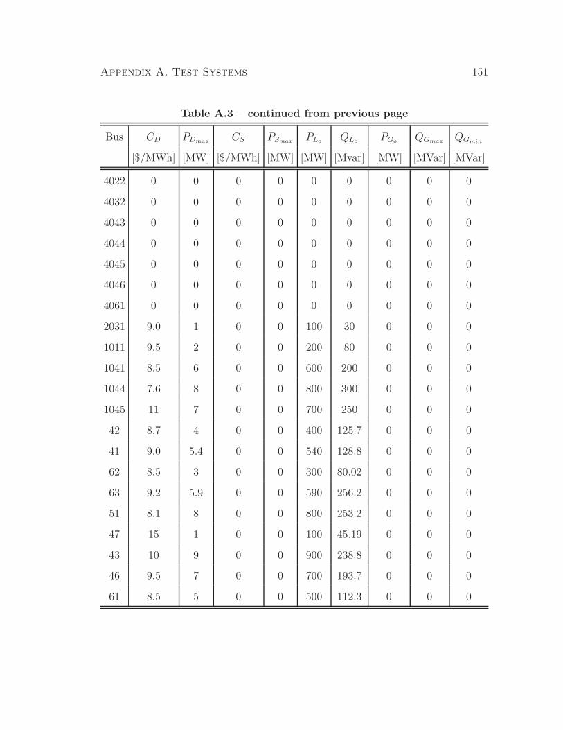
Appendix A. Test Systems 151
Table A.3 – continued from previous page
Bus CD PDmax CS PSmax PLo QLo PGo QGmax QGmin
[$/MWh] [MW] [$/MWh] [MW] [MW] [Mvar] [MW] [MVar] [MVar]
4022 0 0 0 0 0 0 0 0 0
4032 0 0 0 0 0 0 0 0 0
4043 0 0 0 0 0 0 0 0 0
4044 0 0 0 0 0 0 0 0 0
4045 0 0 0 0 0 0 0 0 0
4046 0 0 0 0 0 0 0 0 0
4061 0 0 0 0 0 0 0 0 0
2031 9.0 1 0 0 100 30 0 0 0
1011 9.5 2 0 0 200 80 0 0 0
1041 8.5 6 0 0 600 200 0 0 0
1044 7.6 8 0 0 800 300 0 0 0
1045 11 7 0 0 700 250 0 0 0
42 8.7 4 0 0 400 125.7 0 0 0
41 9.0 5.4 0 0 540 128.8 0 0 0
62 8.5 3 0 0 300 80.02 0 0 0
63 9.2 5.9 0 0 590 256.2 0 0 0
51 8.1 8 0 0 800 253.2 0 0 0
47 15 1 0 0 100 45.19 0 0 0
43 10 9 0 0 900 238.8 0 0 0
46 9.5 7 0 0 700 193.7 0 0 0
61 8.5 5 0 0 500 112.3 0 0 0
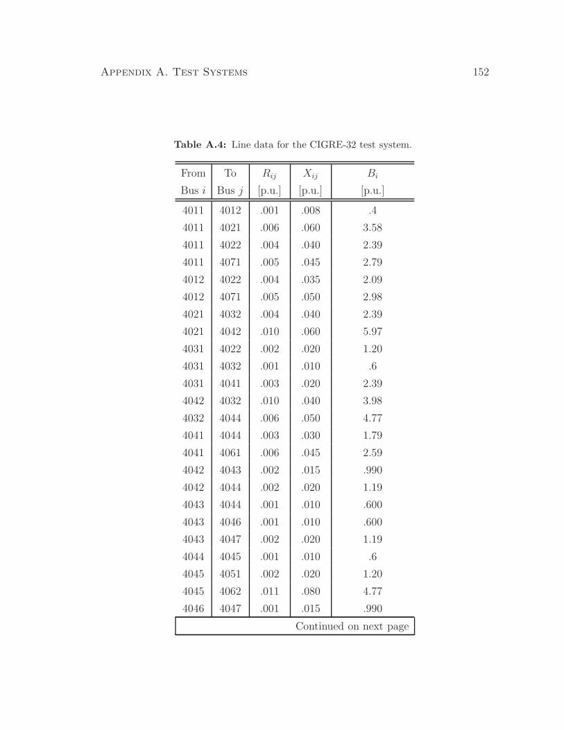
Appendix A. Test Systems 152
Table A.4: Line data for the CIGRE-32 test system.
From To Rij Xij Bi
Bus i Bus j [p.u.] [p.u.] [p.u.]
4011 4012 .001 .008 .4
4011 4021 .006 .060 3.58
4011 4022 .004 .040 2.39
4011 4071 .005 .045 2.79
4012 4022 .004 .035 2.09
4012 4071 .005 .050 2.98
4021 4032 .004 .040 2.39
4021 4042 .010 .060 5.97
4031 4022 .002 .020 1.20
4031 4032 .001 .010 .6
4031 4041 .003 .020 2.39
4042 4032 .010 .040 3.98
4032 4044 .006 .050 4.77
4041 4044 .003 .030 1.79
4041 4061 .006 .045 2.59
4042 4043 .002 .015 .990
4042 4044 .002 .020 1.19
4043 4044 .001 .010 .600
4043 4046 .001 .010 .600
4043 4047 .002 .020 1.19
4044 4045 .001 .010 .6
4045 4051 .002 .020 1.20
4045 4062 .011 .080 4.77
4046 4047 .001 .015 .990
Continued on next page

Appendix A. Test Systems 153
Table A.4 – continued from previous page
From To Rij Xij Bi
Bus i Bus j [p.u.] [p.u.] [p.u.]
4061 4062 .0015 .015 .900
4062 4063 .0015 .015 .900
4071 4072 .0015 .015 3.00
2031 2032 .00599 .045 .050
1011 1013 .00503 .03491 .130
1012 1014 .00710 .04497 .170
1013 1014 .00349 .02503 .100
1021 1022 .01503 .100 .290
1041 1043 .00503 .030 .120
1041 1045 .00751 .060 .240
1042 1044 .01899 .140 .570
1042 1045 .05000 .300 1.13
1043 1044 .00503 .040 .150
1011 4011 0 .008 0
1012 4012 0 .008 0
1022 4022 0 .012 0
1044 4044 0 .005 0
1045 4045 0 .005 0
2031 4031 0 .012 0
4042 42 0 .013 0
4041 41 0 .010 0
4047 47 0 .040 0
4043 43 0 .007 0
4046 46 0 .010 0
4051 51 0 .007 0
4061 61 0 .013 0
Continued on next page

Appendix A. Test Systems 154
Table A.4 – continued from previous page
From To Rij Xij Bi
Bus i Bus j [p.u.] [p.u.] [p.u.]
4062 62 0 .020 0
4063 63 0 .010 0
A.3 1211-bus Test System
A more realistic test system which represents an actual European electric power
system is also used in this thesis to test a proposed model and solution technique.
This test system consists of 1211 buses, 190 generators, and 1567 transmission lines.
The data of this system is not provided because it is confidential.
Bibliography
[1] F. Milano, C. A. Canizares, and M. Invernizzi, “Multi-objective optimization
for pricing system security in electricity markets,” IEEE Transactions on
Power Systems, vol. 18, no. 2, pp. 596–604, May 2003.
[2] “Interim report: Causes of the august 14th blackout in
the united states and canada,” Tech. Rep. [Online]. Available:
http://www.nrcan-rncan.gc.ca/media/docs/814BlackoutReport.pdf
[3] “Report on the events of september 28th, 2003 culminat-
ing in the separation of the italian power system from the
other ucte networks,” Tech. Rep., April 2004. [Online]. Available:
http://www.autorita.energia.it/docs/04/061-04all.pdf
[4] “The black-out in southern sweden and eastern denmark, 23
september, 2003,” Tech. Rep., October 2003. [Online]. Available:
http://www.svk.se/upload/3195/DisturbanceSwedenDenmarkSept23.pdf
[5] M. E. Karystianos, N. G. Maratos, and C. D. Vournas, “Maximizing power-
system loadability in the presence of multiple binding complementarity con-
straints,” IEEE Transactions on Circuits and Systems, vol. 54, no. 8, pp.
1775–1787, August 2007.
[6] W. Rosehart, C. Roman, and A. Schellenberg, “Optimal power flow with
complementarity constraints,” IEEE Transactions on Power Systems, vol. 20,
no. 2, pp. 813–822, May 2005.
155

BIBLIOGRAPHY 156
[7] G. L. Torres and V. H. Quintana, “Power system optimization via successive
linear programming with interior point methods,” University of Waterloo,
Waterloo, ON, Canada, Tech. Rep. UW ECE 93-02, January 1996.
[8] G. D. Irisarri, W. Wang, J. Tong, and S. Mokhtari, “Maximum loadability of
power systems using interior point non-linear optimization method,” IEEE
Transactions on Power Systems, vol. 12, no. 1, pp. 162–169, February 1997.
[9] R. Fuentes-Loyola and V. H. Quintana, “Medium-term hydrothermal coordi-
nation by semidefinite programming,” IEEE Transactions on Power Systems,
vol. 18, no. 4, pp. 1515–1522, November 2003.
[10] M. Madrigal and V. H. Quintana, “Semidefinite programming relaxations for
(0,1)-power dispatch problems,” Power Engineeting Society (PES), summer
meeting, vol. 2, pp. 18–22, 1999.
[11] B. Stott, O. Alsac, and A. J. Monticelli, “Security analysis and optimization,”
in Proceedings of the IEEE, vol. 75, no. 12, December 1987, pp. 1623–1644.
[12] J. Momoh, R. Koessler, M. Bond, and B. Stott, “Challenges to optimal power
flow,” IEEE Transactions on Power Systems, vol. 12, no. 1, pp. 444–447,
February 1997.
[13] “Voltage stability assesment: Concepts, practices and tools,” IEEE/PES
Power System Stability Subcomitte, Tech. Rep., August 2002.
[14] W. D. Rosehart, “Optimal power flows incorporating network stability,” in
Proc. IEEE Power Engineering Society, Winter Meeting, vol. 2, January 2002,
pp. 1100–1104.
[15] G. Irisarri, X. Wang, J. Tong, and S. Mokhtari, “Maximum loadability of
power systems using interior point non-linear optimization method,” IEEE
Transactions on Power Systems, vol. 12, no. 1, pp. 162–172, February 1997,
Siemens Empros Power System Control.

BIBLIOGRAPHY 157
[16] J. Kabouris, C. Vournas, S. Efstathiou, G. Manos, and G. Contaxis, “Voltage
security considerations in an open power market,” in Proc. Electric Utility
Deregulation and Restructuring and Power Technologies, April 2000, pp. 278–
283.
[17] C. A. Canizares, N. Mithulananthan, F. Milano, and J. Reeve, “Linear per-
formance indices to predict oscillatory stability problems in power systems,”
IEEE Transactions on Power Systems, vol. 19, no. 2, pp. 1104–1114, May
2004.
[18] W. Marszalek and Z. W. Trzaska, “Singularity-induced bifurcations in elec-
trical power systems,” IEEE Transactions on Power Systems, vol. 20, no. 1,
pp. 312–320, February 2005.
[19] R. Riaza, S. L. Campbell, and W. Marszalek, “On singular equilibria of index-
1 DAEs,” Circuits Systems Signal Process, vol. 19, no. 2, pp. 131–157, 2000.
[20] V. Ajjarapu and C. Christy, “The continuation power flow: A tool for steady
state voltage stability analysis,” IEEE Transactions on Power Systems, vol. 1,
no. 1, pp. 416–423, February 1992.
[21] C. A. Canizares and F. L. Alvarado, “Point of collapse and continuation
methods for large ac/dc systems,” IEEE Transactions on Power Systems,
vol. 8, no. 1, pp. 1–8, February 1993.
[22] C. A. Canizares, “Calculating optimal system parameters to maximize the
distance to saddle-node bifurcations,” IEEE Transactions on Circuits and
Systems—Part I: Fundamental Theory and Applications, vol. 3, no. 45, pp.
225–237, March 1998.
[23] T. V. Cutsem, “A method to compute reactive power margins with respect
to voltage collapse,” IEEE Transactions on Power Systems, vol. 6, no. 1, pp.
145–155, February 1991.
BIBLIOGRAPHY 158
[24] E. Vaahedi, Y. Mansour, C. Fuchs, S. Granville, M. D. L. Latore, and
H. Hamadanizadeh, “Dynamic security constrained optimal power flow/var
planning,” IEEE Transactions on Power Systems, vol. 16, no. 1, pp. 38–43,
February 2001.
[25] W. D. Rosehart, “Optimization of power systems with voltage security con-
straints,” Ph.D. dissertation, University of Waterloo, Waterloo, ON. Canada,
2000.
[26] W. D. Rosehart, C. A. Canizares, and V. H. Quintana, “Multiobjective opti-
mal power flows to evaluate voltage security cost in power networks,” IEEE
Transactions on Power Systems, vol. 18, no. 2, pp. 578–587, May 2003.
[27] G. L. Torres and V. H. Quintana, “An interior point method for nonlinear op-
timal power flow using voltage rectangular coordinates,” IEEE Transactions
on Power Systems, vol. 13, no. 4, pp. 1211–1218, November 1998.
[28] O. Alsac, J. Bright, M. Paris, and B. Stott, “Further developments in LP-
Based optimal power flow,” IEEE Transactions on Power Systems, vol. 5,
no. 3, pp. 697–711, August 1990, Power Computer Applications Corporation.
[29] M. Huneault and F. Galiana, “A survey of the optimal power flow literature,”
IEEE Transactions on Power Systems, vol. 6, no. 2, pp. 762–770, May 1991.
[30] J. Kubokawa, H. Sasaki, S. Ahmed, and G. Strbac, “Application of optimal
power flow for voltage stability problem,” in Proc. International Conference
on Electric Power Engineering, Budapest, May 1999, pp. 134–141.
[31] W. Rosehart, C. Canizares, and V. Quintana, “Optimal power flow incorpo-
rating voltage collapse constraints,” in Proc. IEEE Power Engineering Soci-
ety, Summer Meeting, vol. 2, July 1999, pp. 820–825.
[32] F. Milano, C. A. Canizares, and A. J. Conejo, “Sensitivity-based security-
constrained OPF market clearing model,” IEEE Transactions on Power Sys-
tems, vol. 20, no. 4, pp. 2051–2059, November 2005.
BIBLIOGRAPHY 159
[33] A. Berizzi, C. Bovo, M. Innorta, and P. Marannino, “Multiobjective opti-
mization techniques applied to modern power systems,” in Power Engineer-
ing Society Winter Meeting, vol. 3, Columbus, OH, USA, February 2001, pp.
1503–1508.
[34] S. K. M. Kodsi and C. A. Canizares, “Application of a stability-constrained
optimal power flow to tuning of oscillation controls in competitive electricity
markets,” IEEE Transactions on Power Systems, accepted for Publication
March 2007.
[35] H. Harsan, N. Hadjsaid, and P. Pruvot, “Cyclic security analysis for secu-
rity constrained optimal power flow,” IEEE Transactions on Power Systems,
vol. 12, no. 2, pp. 948–953, May 1997, Electricite de France.
[36] A. J. Wood and B. R. Wollenberg, Power Generation, Operation, and Control,
2nd ed. John Wiley and Sons, 1996.
[37] A. I. Cohen, V. Brandwajn, and S. K. Chang, “Security constrained unit
commitment for open markets,” in Proc. IEEE International Conference
PICA’99, P. I. C. Applications, Ed., May 1999, pp. 39–44, ABB Systems
Control.
[38] J. J. Shaw, “A direct method for security-constrained unit commitment,”
IEEE Transactions on Power Systems, vol. 10, no. 3, pp. 1329–1342, August
1995, ALPHATECH.
[39] D. Hur, J.-K. Park, B. H. Kim, and K.-M. Son, “Security constrained optimal
power flow for the evaluation of transmission capability on Korea electric
power system,” in Proc. IEEE Power Engineering Society, Summer Meeting,
vol. 2, July 2001, pp. 1133–1138.
[40] P. Yang and A. Sekar, “A new approach to security-constrained optimal power
flow analysis,” in Proc. IEEE Power Engineering Society, Summer Meeting,
vol. 3, July 2001, pp. 1462–1467.
BIBLIOGRAPHY 160
[41] C. A. Canizares, H. Chen, and W. Rosehart, “Pricing system security in
electricity markets,” Proc. Bulk Power Systems Dynamics and Control-V.,
August 2001.
[42] W. Rosehart, C. Canizares, and V. Quintana, “Costs of voltage security
in electricity markets,” in Proc. IEEE Power Engineering Society, Summer
Meeting, vol. 4, Seattle, WA, July 2000, pp. 2115–2120.
[43] F. Milano, C. A. Canizares, and M. Invernizzi, “Voltage stability constrained
OPF market models considering N-1 contingency criteria,” Electric Power
System Research, vol. 74, no. 1, pp. 27–36, March 2005.
[44] P. Lof, T. Smed, G. Andersson, and D. Hill, “Fast calculation of a voltage
stability index,” IEEE Transactions on Power Systems, vol. 7, no. 1, pp.
54–64, February 1992.
[45] A. Tiranuchit and R. Thomas, “A posturing strategy againts voltage instabil-
ities in electric power systems,” IEEE Transactions on Power Systems, vol. 3,
no. 1, pp. 87–93, February 1988.
[46] G. Huang and T. Zhu, “A new method to find the voltage collapse point,” in
Proc. IEEE Power Engineering Society, Summer Meeting, vol. 2, July 1999,
pp. 1324–1329.
[47] A. C. Z. de Souza, “New techniques to efficiently determine proximity to static
voltage collapse,” Ph.D. dissertation, University of Waterloo, Waterloo, ON.
Canada, 1996.
[48] N. Mithulananthan, “Hopf bifurcation control and indices for power system
with interacting generator and facts controllers,” Ph.D. dissertation, Univer-
sity of Waterloo, Waterloo, ON. Canada, 2002.
[49] A. Berizzi, P. Finazzi, D. Dosi, P. Marannino, and S. Corsi, “First and second
order methods for voltage collapse assessment and security enhancement,”
IEEE Transactions on Power Systems, vol. 13, no. 2, pp. 543–551, May 1998.
BIBLIOGRAPHY 161
[50] A. Berizzi, P. Bresesti, P. Marannino, G. Granelli, and M. Montagna,
“System-area operating margin assessment and security enhancement againts
voltage collapse,” IEEE Transactions on Power Systems, vol. 11, no. 3, pp.
1451–1461, August 1996.
[51] M. Haque, “Determination of steady-state voltage stability limt using P-Q
curve,” IEEE Power Engineering Review, pp. 71–72, April 2002.
[52] J. Kubokawa, R. Inoue, and H. Sasaki, “A solution of optimal power flow with
voltage stability constraints,” in Proc. International Conference on Power
System Technology, December 2000, pp. 625–630.
[53] C. Canizares, W. Rosehart, A. Berizzi, and C. Bovo, “Comparison of voltage
security constrained optimal power flow techniques,” in Proc. IEEE Power
Engineering Society, Summer Meeting, vol. 4, no. 2, Vancouver, BC., July
2001, pp. 2115–2120.
[54] P. Kundur, J. Paserba, V. Ajjarapu, G. Anderson, A. Bose, C. Canizares,
et al., “Definition and clasification of power system stability,” IEEE Trans-
actions on Power Systems, vol. 19, no. 2, pp. 1387–1401, May 2004.
[55] P. Kundur, Power System Stability and Control, ser. Power System Engineer-
ing. McGraw-Hill, 1994.
[56] J. Machowski, J. W. Bialek, and J. R. Bumby, Power System Dynamics and
Stability. John Wiley and Sons, 1997.
[57] D. J. Hill and I. M. Y. Mareels, “Stability theory for differential/algebraic
systems with application to power systems,” IEEE Transactions on Circuits
and Systems, vol. 37, no. 11, pp. 1416–1423, November 1990.
[58] V. Venkatasubramanian, H. Schattler, and J. Zaborszky, “A taxonomy theory
of the dynamics of large power systems with emphasis on its voltage stability,”
in Bulk Power System Voltage Phenomena II-Voltage Stability and Security,
L. H. Fink, Ed., August 1991, pp. 9–52.
BIBLIOGRAPHY 162
[59] R. Seydel, Practical Bifurcation and Stability Analysis: from equilibrium to
chaos, 2nd ed. Springer-Verlag, 1994.
[60] I. Dobson and H. D. Chiang, “Towards a theory of voltage collapse in electric
power systems,” Systems & Control Letters, vol. 13, pp. 253–262, 1989.
[61] C. A. Canizares, “Conditions for saddle-node bifurcations in ac/dc power sys-
tems,” International Journal of Electrical Power and Energy Systems, vol. 17,
no. 1, pp. 61–68, January 1995.
[62] I. Dobson and L. Lu, “Voltage collapse precipitated by the immediate change
in stability when generator reactive power limits are encountered,” IEEE
Transactions on Circuits and Systems—Part I: Fundamental Theory and Ap-
plications, vol. 39, no. 9, pp. 762–766, September 1992.
[63] V. Venkatasubramanian, H. Schattler, and J. Zaborszky, “Dynamics of large
constrained nonlinear systems-a taxonomy theory,” in Proceedings of the
IEEE, vol. 83, no. 11, November 1995, pp. 1530–1560.
[64] N. Balu, T. Bertram, A. Bose, V. Brandwajn, G. Cauley, D. Curtice,
A. Fouad, L. Fink, M. G. Lauby, B. F. Wollember, and J. N. Wrubel, “On-
Line power system security analysis,” in Proceedings of the IEEE, vol. 80,
no. 2, February 1992, pp. 262–280.
[65] M. Shahidehpour, W. F. Tinney, and Y. Fu, “Impact of security on power
systems operation,” in Proceedings of the IEEE, vol. 93, no. 11, November
2005, pp. 2013–2025.
[66] North American Electric Reliability Council, “Available transfer capa-
bility definitions and determination,” June 1996. [Online]. Available:
http://www.westgov.org/wieb/wind/06-96NERCatc.pdf
[67] E. W. King, C. A. Canizares, and H. Chen, “A probabilistic approach to
evaluate security costs and levels in competitive electricity markets,” in Bulk

BIBLIOGRAPHY 163
Power Systems Dynamics and Control, vol. 6, Cortina d’Ampezzo, Italy, 2004,
pp. 16–23.
[68] I. Dobson, S. Greene, R. Rajaraman, C. L. DeMarco, F. L. Alvarado,
M. Glavic, J. Zhang, and R. Zimmerman, “Electric power transfer
capability: Concepts, applications, sensitivity and uncertainty,” Power
Systems Engineering Research Center PSerc, vol. 1, no. 34, November 2001.
[Online]. Available: http://www.pserc.cornell.edu/tcc/
[69] A. R. Bergen and V. Vittal, Power Systems Analysis, 2nd ed. Prentice Hall,
2000.
[70] G. Ejebe, J. Tong, J. Waight, J. Frame, X. Wang, and W. Tinney, “Avail-
able transfer capability calculations,” IEEE Transactions on Power Systems,
vol. 13, no. 4, pp. 1521–1527, November 1998.
[71] C. A. Canizares, “Applications of optimization to voltage collapse analysis,”
in IEEE/PES Summer Meeting, San Diego, CA., July 1998, pp. 1–8, panel
Session: “Optimization Techniques in Voltage Collapse Analysis”.
[72] ——, “UWPFLOW.” [Online]. Available:
http://thunderbox.uwaterloo.ca/∼claudio/software/pflow.html
[73] H. Y. Benson, D. F. Shanno, and R. J. Vanderbei, “Interior-point methods
for nonconvex nonlinear programming: Complementarity constraints,” Oper-
ations Research and Financial Engineering, pp. 1–20, September 2002.
[74] F. Milano, “Pricing system security in electricity markets models with inclu-
sion of voltage stability constraints,” Ph.D. dissertation, University of Gen-
ova, Genova, Italy, April 2003.
[75] S. Hunt, Making competition work in electricity, J. Wiley, Ed. Wiley Finance,
2002.
[76] [Online]. Available: http://www.econ100.com/eu5e/open/glossary.html
BIBLIOGRAPHY 164
[77] G. B. Alderete, “Alternative models to analyze market power and financial
transmission rights in electricity markets,” Ph.D. dissertation, University of
Waterloo, Waterloo, ON. Canada, 2005.
[78] S. Stoft, Power System Economics, J. Wiley, Ed. IEEE press, 2002.
[79] K. Xie, Y. H. Song, J. Stonham, E. Yu, and G. Liu, “Decomposition model
and interior point methods for optimal spot pricing of electricity in deregu-
lation environments,” IEEE Transactions on Power Systems, vol. 15, no. 1,
pp. 39–50, February 2000.
[80] V. H. Quintana and G. L. Torres, Introduction to Interior-Point Methods,
University of Waterloo, Waterloo, On. Canada.
[81] G. L. Torres and V. H. Quintana, “Rectangular and polar optimal power flow
by a primal-dual interior-point method for nonliner programming,” University
of Waterloo, Canada, Technical Report UW ECE 97-13, November 1997.
[82] H. Wolkowicz, R. Saigal, and L. Vandenberghe, Eds., Handbook of Semidefi-
nite Programming. Springer, 2000, vol. 27.
[83] L. Vandenberghe and S. Boyd, “Semidefinite programming,” SIAM review,
vol. 38, no. 1, pp. 49–95, March 1996.
[84] M. F. Anjos, “Towards and SDP-based algorithm for the satisfiability prob-
lem,” Operational Research Group, School of Mathematics. University of
Southampton. U.K.
[85] C. D. Vournas, M. Karystianos, and N. G. Maratos, “Bifurcation points and
loadability limits as solutions of constrained optimization problems,” in Proc.
IEEE-PES, Summer Meeting, vol. 3, July 2000, pp. 1883–1888.
[86] N. G. Maratos and C. D. Vournas, “Relationships between static bifurcations
and constrained optima,” in ISCAS 2000, vol. 2, Geneva, Switzerland, May
2000, pp. 477–480.

BIBLIOGRAPHY 165
[87] I. Dobson, “Observations on the geometry of saddle node bifurcations and
voltage collapse in electrical power systems,” IEEE Transactions on Circuits
and Systems—Part I: Fundamental Theory and Applications, vol. 39, no. 3,
pp. 240–243, March 1992.
[88] J. Nocedal and S. J. Wright, Numerical Optimization. Springer, 1999.
[89] C. A. Canizares, F. L. Alvarado, C. L. DeMarco, I. Dobson, and W. F.
Long, “Point of collapse methods applied to ac/dc power systems,” IEEE
Transactions on Power Systems, vol. 2, no. 7, pp. 673–683, May 1992.
[90] C. D. Vournas, B. M. Nomikos, D. N. Makridou, M. E. Karystianos, and G. A.
Manos, “Bifurcation analysis of electrical power systems,” January 2000, pre-
sented in the 1st Interdisciplinary Symposium of Nonlinear Problems, NTUA,
Athens.
[91] F. Zhang, The Schur Complement and Its Applications. Springer, 2005.
[92] E. Castillo, A. J. Conejo, C. Castillo, R. Mınguez, and D. Ortigosa, “Per-
turbation approach to sensitivity analysis in mathematical programming,”
J. Optimization Theory and Applications, vol. 128, no. 1, p. 49–74, January
2006.
[93] R. Fourer, D. M. Gay, and B. W. Kernighan, AMPL A Modeling Language
for Mathematical Programming, 2nd ed. Thomson, 2003.
[94] M. C. Ferris, R. Fourer, and D. M. Gay, “Expressing complementarity
problems in an algebraic modeling languange and communicating them to
solvers.” [Online]. Available: www.ampl.com
[95] “KNITRO.” [Online]. Available: http://www.ziena.com
[96] R. A. Horn and C. R. Johnson, Matrix Analysis. Cambridge University
Press, 1985.
BIBLIOGRAPHY 166
[97] J. Arrillaga and C. Arnold, Computer Analysis of Power Systems. John
Wiley and Sons, 1990.
[98] Ipopt (Interior Point Optimizer). [Online]. Available:
http://homes.esat.kuleuven.be/∼optec/software/ipopt/index.html
[99] Matlab. [Online]. Available: http://www.mathworks.com/
[100] X. Yan and V. H. Quintana, “Improving an interior-point-based OPF by
dynamic adjustments of step sizes and tolerances,” IEEE Transactions on
Power Systems, vol. 14, no. 2, pp. 709–717, May 1999.
[101] R. J. Avalos, C. A. Canizares, F. Milano, and A. J. Conejo, “Equivalency of
continuation and optimization methods to determine saddle-node and limit-
induced bifurcations in power systems,” IEEE Transactions on Circuits and
Systems—Part I: Fundamental Theory and Applications, May 2008. [Online].
Available: http://thunderbox.uwaterloo.ca/∼claudio/papers/Rafael1.pdf
[102] R. J. Avalos, C. A. Canizares, and M. F. Anjos, “Practical solution of voltage-
stability-constrained optimal power flows,” IEEE Transactions on Power Sys-
tems, 2007, 12 pages, manuscript submitted for review on November 21, 2007.
[103] ——, “A practical voltage-stability-constrained optimal power flow,” in IEEE
PES General Meeting, Pittsburgh, USA, July 2008, invited paper. [Online].
Available: http://thunderbox.uwaterloo.ca/∼claudio/papers/RafaelGM.pdf