Analysis and Design of Telecommunications Systems:

prerequisite

Marc Van Droogenbroeck

Abstract

This document is the prerequisite for Analysis and Design of Telecommunications Systemstaught at the University of Liège. It is intended to be a reminder of some basic knowledge.

For a textbook, I recommend: Digital and Analog Communication Systems, by L. Couch,Prentice Hall [1].

1

Contents

1 Fourier transform and spectrum analysis 3

1.1 Properties . . . . . . . . . . . . . . . . . . . . . . . . . . . . . . . . . . . . . . . . 3

1.2 Specic signals . . . . . . . . . . . . . . . . . . . . . . . . . . . . . . . . . . . . . . 4

1.3 Fourier transform pairs . . . . . . . . . . . . . . . . . . . . . . . . . . . . . . . . 5

2 Signals 6

2.1 Continuous-time and discrete-time signals . . . . . . . . . . . . . . . . . . . . . . . 6

2.2 Analog and digital signals . . . . . . . . . . . . . . . . . . . . . . . . . . . . . . . . 6

2.3 Energy and power . . . . . . . . . . . . . . . . . . . . . . . . . . . . . . . . . . . . 6

2.4 Deterministic vs stochastic tools . . . . . . . . . . . . . . . . . . . . . . . . . . . . 7

2.5 Decibel . . . . . . . . . . . . . . . . . . . . . . . . . . . . . . . . . . . . . . . . . . 8

2.6 Digitization of analog signals . . . . . . . . . . . . . . . . . . . . . . . . . . . . . . 8

2.6.1 Sampling theorem . . . . . . . . . . . . . . . . . . . . . . . . . . . . . . . . 8

2.6.2 Impulse sampling . . . . . . . . . . . . . . . . . . . . . . . . . . . . . . . . . 9

3 Linear systems 10

3.1 Linear time-invariant systems . . . . . . . . . . . . . . . . . . . . . . . . . . . . . . 10

3.2 Impulse response and transfer function . . . . . . . . . . . . . . . . . . . . . . . . . 10

3.3 Distortionless transmission . . . . . . . . . . . . . . . . . . . . . . . . . . . . . . . . 10

4 Random variables and stochastic processes 11

4.1 Gaussian random variable . . . . . . . . . . . . . . . . . . . . . . . . . . . . . . . . 11

4.2 Stochastic processes . . . . . . . . . . . . . . . . . . . . . . . . . . . . . . . . . . . 11

4.2.1 Stationarity . . . . . . . . . . . . . . . . . . . . . . . . . . . . . . . . . . . 11

4.2.2 Power spectral density and linear systems (= ltering) . . . . . . . . . . . . 13

4.2.3 Noise and white noise . . . . . . . . . . . . . . . . . . . . . . . . . . . . . . 13

5 Line coding and spectra 15

5.1 Line coding . . . . . . . . . . . . . . . . . . . . . . . . . . . . . . . . . . . . . . . . 15

5.2 General formula for the power spectral density of baseband digital signals . . . . . 15

6 Power budget link for radio transmissions 17

7 Information theory 18

7.1 Channel capacity . . . . . . . . . . . . . . . . . . . . . . . . . . . . . . . . . . . . 18

7.2 On the importance of the EbN0

ratio for digital transmissions . . . . . . . . . . . . . 18

2

1 Fourier transform and spectrum analysis

Denition 1. [Fourier transform] Let g(t) be a deterministic signal (also called a waveform),the Fourier transform of g(t), denoted G, is

G(f) =

∫ +∞

−∞g(t)e−2πjftdt (1.1)

where f is the frequency parameter with units in Hertz, Hz (that is 1s ). It is also related to angular

pulsation ω by ω = 2πf .

Note that f is the parameter of the Fourier transform G(f), that is also called (two-sided)spectrum of g(t), because it contains both positive and negative components.

Denition 2. [Inverse Fourier transform] The time waveform g(t) is obtained by takingthe inverse Fourier transform of G(f), dened as follows

g(t) =

∫ +∞

−∞G(f)e2πjftdt (1.2)

The functions g(t) and G(f) are said to constitute a Fourier transform pair, because they aretwo representations of a same signal.

1.1 Properties

Proposition 3. [Spectral symmetry of real signals] If g(t) is real, then

G(−f) = G∗(f) (1.3)

where ()∗ denotes the conjugate operation.

A consequence is that the negative components can be obtained from the positives ones. Therefore,the positive components are sucient to describe the original waveform g(t).

Proposition 4. [Rayleigh] The total energy in the time domain and the frequency domain areequal:

E =

∫ +∞

−∞|g(t)|2 dt =

∫ +∞

−∞‖G(f)‖2 df (1.4)

After integration, ‖G(f)‖2 provides the total energy of the signal in Joule, J . Therefore, it issometimes named energy spectral density.

Proposition 5. [Linearity] If g(t) = c1g1(t) + c2g2(t) then G(f) = c1G1(f) + c2G2(f).

This property of linearity is essential in telecommunications, because most systems (channels,lters, etc) are linear. The consequence is that any linear system can only modify the spectralcontent a signal, but is incapable to add new frequencies.

This property also highlights that a spectrum analysis is adequate for dealing with linear systems.To the contrary, it is more dicult to analyze a non-linear system (for example a squaring operator,g2(t)) in terms of frequencies.

3

Operation Function Fourier transform

Conjugate symmetry g(t) is real G(f) = G∗(−f)

Linearity c1g1(t) + c2g2(t) c1G1(f) + c2G2(f)

Time scaling g(at) 1|a|G

(fa

)Time shift (delay) g(t− t0) G(f) e−2πjft0

Convolution g(t)⊗ h(t) =∫ +∞−∞ g(τ)h(t− τ) dτ G(f)H(f)

Frequency shift g(t) e2πjfct G (f − fc)

Modulation g(t) cos (2πfct)G(f−fc)+G(f+fc)

2

Temporal derivation ddtg(t) 2πjf G(f)

Temporal integration∫ t−∞ g(τ) dτ 1

2πjf G(f)

Table 1: Main properties of the Fourier transform.

1.2 Specic signals

Some waveforms play a specic role in communications.

1. The Dirac delta function, denoted δ(t), is dened by

δ(t) =

∞, x = 00 x 6= 0

(1.5)

and ∫ +∞

−∞δ(t) dt = 1 (1.6)

The Dirac delta function is not a true function, so it is said to be a singular function.However, it is considered as a function in the more general framework of the theory ofdistributions. Note that

g(t)⊗ δ(t) = g(t) (1.7)

According to equation 1.6, ∫ +∞

−∞δ(t)e−2πjft = e0 = 1 (1.8)

As a consequence, 1 is the Fourier transform of δ(t). Likewise, δ(f) is the Fouriertransform of 1. This explains the central role of the Dirac delta function in signal processingand communications.The Dirac delta function is also called the unit impulse function.

2. Rectangular pulse

rect(t) =

1 − 1

2 < t < 12

0 |t| > 12

(1.9)

The rectangular pulse is the most common shape form for the representation of digitalsignals.

3. Step function (Heaviside function)

u(t) =

1 t > 00 t < 0

(1.10)

4

4. Sign function

sign(t) =

1 t > 0−1 t < 0

(1.11)

5. Sinc function

sinc(t) =sin(πt)

πt(1.12)

1.3 Fourier transform pairs

Temporal waveform Fourier transform

δ(t) 1

1 δ(f)

cos(2πfct)12 [δ(f − fc) + δ(f + fc)]

sin(2πfct)12j [δ(f − fc)− δ(f + fc)]

rect(tT

)T sinc(fT )

sinc(2Wt) 12W rect

(f

2W

)sign(t) 1

πjf

u(t) 12δ(f) + 1

2πjf

1πt −j sign(f)∑+∞

i=−∞ δ (t− iT0) 1T0

∑+∞n=−∞ δ

(f − n

T0

)e−πt

2

e−πf2

e−atu(t), a > 0 1a+2πjf

e−a|t|, a > 0 2aa2+(2πf)2

Table 2: Some common Fourier transform pairs.

5

2 Signals

2.1 Continuous-time and discrete-time signals

A continuous-time signal g(t) is a signal of the real variable t (time). For example, the signalcos(2πfct) is a function of time.

A discrete-time signal g[n] is a sequence where the values of the index n are integers. Such a signalcarries digital information.

2.2 Analog and digital signals

An analog signal is a signal with a continuous range of amplitudes.

A digital signal is a member of a set ofM unique signals, dened over the T period, that representM data symbols.

Figure 2.1 represents an analog and a digital signal (top row). In practice, digital signals arematerialized by a continuous-time signal, named a representation. Such representations areillustrated in Figure 2.1 (bottom row).

1 0 1 0 1 1

Analog information signal Digital information signal

Analog representation Digital representation

-1

-0.5

0

0.5

1

1.5

2

0 2 4 6 8 10

-2

-1.5

-1

-0.5

0

0.5

1

1.5

2

0 2 4 6 8 10-0.5

0

0.5

1

1.5

0 1 2 3 4 5 6-1.5

-1

-0.5

0

0.5

1

1.5

0 1 2 3 4 5 6

Figure 2.1: Examples of representations of an continuous-time signal (left) and a discrete-timesignal (right).

2.3 Energy and power

The power in watts [W ] delivered by a voltage signal v(t) in volts to a resistive load R in ohms[Ω] is given by

P = v(t) i(t) =v2(t)

R= R i2(t) (2.1)

6

where i(t) is the current.

In communications, the value of the resistive load is normalized to 1 [Ω]. Therefore, the instanta-neous normalized power is given by

p(t) = v2(t) = i2(t) (2.2)

The averaged normalized power is given by

P = limT→∞

1

2T

∫ T

−Tv2(t) dt (2.3)

A signal v(t) is called a power signal if and only if its averaged power is non-zero and nite, thatis 0 < P <∞.

Example 6. Power of a sinusoid A cos (2πfct). The averaged normalized power delivered to a1 [Ω] load is

P = limT→∞

1

2T

∫ T

−TA2 cos2 (2πfct) dt (2.4)

= limT→∞

A2

4T

∫ T

−T(1 + cos(4πfct) dt (2.5)

=A2

2+ limT→∞

A2

4T

(sin (4πfcT )

4πfc− sin (−4πfcT )

4πfc

)(2.6)

=A2

2+A2

2limT→∞

sin (4πfcT )

4πfcT=A2

2(2.7)

Therefore, A2

2 is the power of a sinusoid A cos (2πfct). The sinusoid is a power signal.

The energy in Joules of a voltage signal v(t) in volts is given by

E =

∫ +∞

−∞v2(t) dt (2.8)

A signal v(t) is called an energy signal if and only if its energy is non-zero and nite, that is0 < E <∞.

2.4 Deterministic vs stochastic tools

As shown in Figure 2.2, the deterministic or stochastic nature of signals depends on the signal andthe location in the communication chain.

transmitter receiver

User's signal deterministic stochasticNoise and interference stochastic stochastic

Figure 2.2: Deterministic or stochastic nature of signals.

In fact, only the user's signal at the transmitter is fully known; it would make no sense to senda signal that would be known by the receiver, at least from a communication engineer's point ofview.

Therefore, we need to adapt the tools for describing signals to their intrinsic nature. More precisely,it appears that stochastic signals can only be described in terms of statistics (mean, average,autocorrelation function, etc).

Figure 2.3 presents the tools used for describing the power of a signal according to its intrinsicnature.

7

deterministic stochastic

signal to consider voltage / current powerpower analysis instantaneous power Power Spectral Density (PSD)

p(t) = |v(t)|2R = R |i(t)|2 E

X2(t)

=∫ +∞−∞ γX(f)df

Figure 2.3: Description of power adapted to the intrinsic nature of signals.

2.5 Decibel

The decibel is a base 10 logarithm measure, used mainly for powers:

x ↔ 10 log10(x) [dB] (2.9)

When describing powers, decibels should be expressed in dB of watts: dBW . Note that dB isoften a shortcut of dBW .

Typical values are given in the following table:

x [W ] 10 log10(x) [dBW ]

1 [W ] 0 [dBW ]2 [W ] 3 [dBW ]

0, 5 [W ] −3 [dBW ]5 [W ] 7 [dBW ]

10n [W ] 10× n [dBW ]

Example 7. Power conversion in [dB]. Assume P = 25 [W ]. Because 25 = 100/2/2, we have that

10 log10(25) = 10 log10(100)− 10 log10(2)− 10 log10(2) (2.10)

= 20− 3− 3 = 14 [dBW ] (2.11)

2.6 Digitization of analog signals

A waveform g(t) is said to be band-limited to B hertz if

G(f) = 0, for |f | ≥ B (2.12)

2.6.1 Sampling theorem

Theorem 8. [Shannon] Any physical waveform w(t), band-limited to B hertz, can be entirelyrepresented by the following samples series

g

[n

fs

](2.13)

where n is an integer and fs is the sampling, if

fs ≥ 2B (2.14)

The condition fs ≥ 2B is named the Nyquist criterion.

8

2.6.2 Impulse sampling

The impulse-sampled series of a waveform is obtained by multiplying it with a train of unit-weightimpulses:

gs(t) = g(t)

+∞∑n=−∞

δ (t− nTs) (2.15)

The Fourier transform of gs(t) is then

Gs(f) = G(f)⊗ 1

Ts

+∞∑n=−∞

δ

(f − n

Ts

)(2.16)

= fs

+∞∑n=−∞

G (f − nfs) (2.17)

The spectrum of the impulse sampled signal is the spectrum of the unsampled signal that isrepeated every fs Hz, where fs is the sampling frequency. This is shown in Figure 2.4.

Figure 2.4: Eects of impulse sampling on a waveform w(t) [1].

9

3 Linear systems

3.1 Linear time-invariant systems

An electronic lter or system ψ (t) is linear when the principle of superposition holds. That iswhen the output y(t) to a combination of inputs follows

y(t) = ψ (ag1(t) + bg2(t)) = aψ (g1(t)) + bψ (g2(t)) (3.1)

The system ψ (t) is time-invariant if, for any delayed input g(t− τ), the output is also delayed bythe same amount y(t− τ).

3.2 Impulse response and transfer function

The impulse response to a lter is the response h(t) when the input is a forcing Dirac deltafunction.

The transfer function or frequency response is the Fourier transform of the impulse response,H.

Using the convolution theorem, we get that if y(t) is the output of a lter expressed by its impulseresponse h(t) to an input g(t), then

Y(f) = H(f)G(f) (3.2)

3.3 Distortionless transmission

In communication, a distortionless channel or ideal channel is a channel whose output is a pro-portion of the delayed version of the input

y(t) = Ag(t− τ) (3.3)

The corresponding frequency response of an ideal channel is then

Y(f)

G(f)= Ae−2πjfτ (3.4)

10

4 Random variables and stochastic processes

4.1 Gaussian random variable

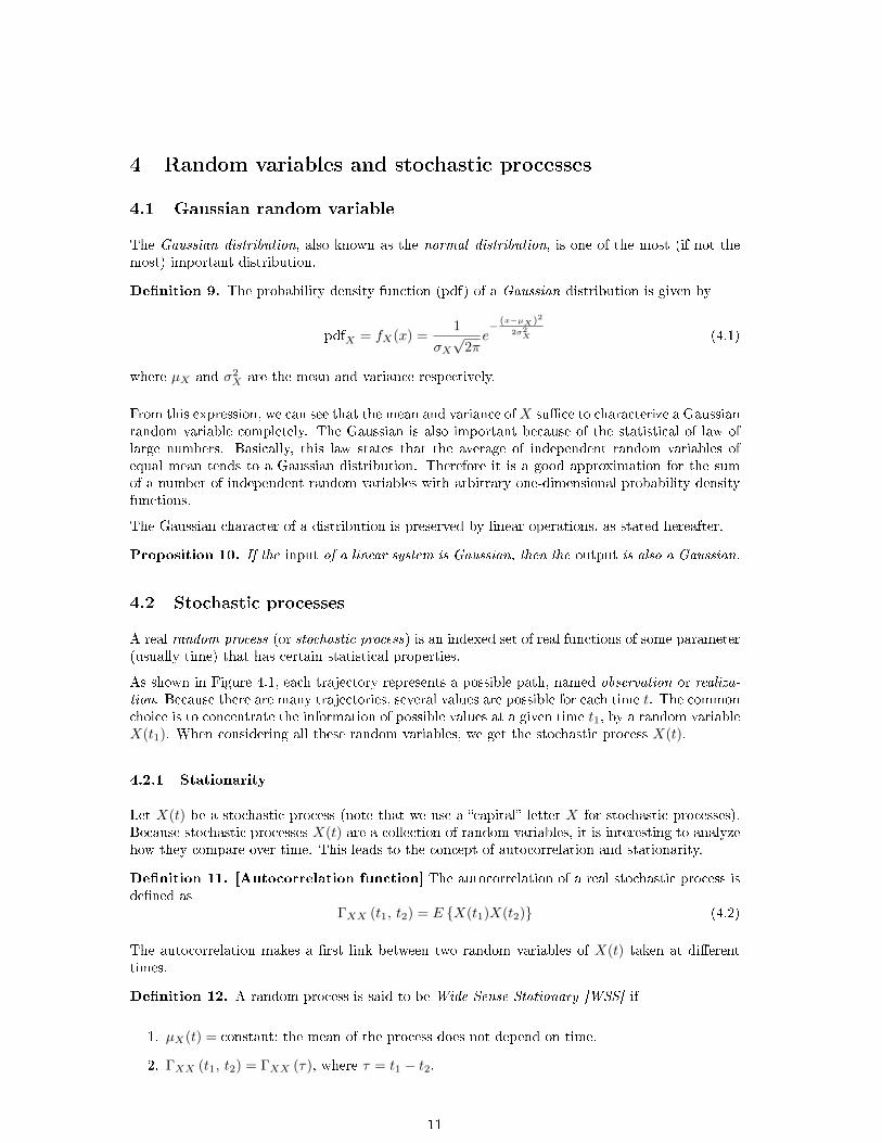
The Gaussian distribution, also known as the normal distribution, is one of the most (if not themost) important distribution.

Denition 9. The probability density function (pdf) of a Gaussian distribution is given by

pdfX = fX(x) =1

σX√

2πe− (x−µX)2

2σ2X (4.1)

where µX and σ2X are the mean and variance respectively.

From this expression, we can see that the mean and variance ofX suce to characterize a Gaussianrandom variable completely. The Gaussian is also important because of the statistical of law oflarge numbers. Basically, this law states that the average of independent random variables ofequal mean tends to a Gaussian distribution. Therefore it is a good approximation for the sumof a number of independent random variables with arbitrary one-dimensional probability densityfunctions.

The Gaussian character of a distribution is preserved by linear operations, as stated hereafter.

Proposition 10. If the input of a linear system is Gaussian, then the output is also a Gaussian.

4.2 Stochastic processes

A real random process (or stochastic process) is an indexed set of real functions of some parameter(usually time) that has certain statistical properties.

As shown in Figure 4.1, each trajectory represents a possible path, named observation or realiza-tion. Because there are many trajectories, several values are possible for each time t. The commonchoice is to concentrate the information of possible values at a given time t1, by a random variableX(t1). When considering all these random variables, we get the stochastic process X(t).

4.2.1 Stationarity

Let X(t) be a stochastic process (note that we use a capital letter X for stochastic processes).Because stochastic processes X(t) are a collection of random variables, it is interesting to analyzehow they compare over time. This leads to the concept of autocorrelation and stationarity.

Denition 11. [Autocorrelation function] The autocorrelation of a real stochastic process isdened as

ΓXX (t1, t2) = E X(t1)X(t2) (4.2)

The autocorrelation makes a rst link between two random variables of X(t) taken at dierenttimes.

Denition 12. A random process is said to be Wide-Sense Stationary [WSS] if

1. µX(t) = constant; the mean of the process does not depend on time.

2. ΓXX (t1, t2) = ΓXX (τ), where τ = t1 − t2.

11

t

t

t

ω1

ω2

ωn

X(t, ω1)X(tk, ω1)

X(tk, ω2)X(t, ω2)

X(t, ωn)

Observation space Ω

X(tk, ωn)tk

Figure 4.1: Possible trajectories of a stochastic process.

The autocorrelation function of stationary stochastic processes is an essential tool because, forτ = 0, it expresses the average power:

ΓXX (τ = 0) = EX2(t)

(4.3)

In practice, we thus consider that the power PX of a stochastic process is given by:

PX = EX2(t)

(4.4)

Consequently, the Fourier transform of the autocorrelation provides the power distribution inthe frequency domain. This leads to the notion of power spectral density of wide-sense stationarystochastic processes as dened hereafter.

Denition 13. [Power spectrum or power spectral density of a stationary process]

γX(f) =

∫ +∞

−∞ΓXX (τ) e−2πjfτdτ (4.5)

In practice,

PX = EX2(t)

=

∫ +∞

−∞γX(f)df (4.6)

Therefore, γX(f) expresses the contribution of each frequency to the total power.

Example 14. Let us consider a signal with a random phase θ ∈ [0, 2π] or [−π,+π]

X(t) = Ac cos (2πfct+ Θ) (4.7)

12

This is typical for the carrier signal of a modulated signal. The mean of X(t) is computed as

µX(t) = E X(t) =

∫ +π

−πAc cos (2πfct+ θ)

1

2πdθ = 0 (4.8)

The autocorrelation is obtained as follows:

ΓXX (t1, t2) = E X(t1)X(t2) (4.9)

=

∫ +π

−πAc cos (2πfct1 + θ)Ac cos (2πfct2 + θ)

1

2πdθ (4.10)

=A2c

2cos [2πfc(t2 − t1)] =

A2c

2cos [2πfcτ ] (4.11)

We then conclude that the signal is wide-sense stationary and compute its power spectral density:

γX(f) =A2c

4[δ(f − fc) + δ(f + fc)] (4.12)

4.2.2 Power spectral density and linear systems (= ltering)

Consider a wide-sense stationary process X(t), a linear system whose transfer function is given byH(f), and Y (t) the output process.

Theorem 15. The mean of Y (t) is given by:

µY = µXH(0) (4.13)

Denition 16. [Wiener-Kintchine] The power spectral density Y (t) is given by:

γY (f) = ‖H(f)‖2 γX(f) (4.14)

In addition, if the stochastic process X(t) is Gaussian, then the ltered output Y (t) is also Gaus-sian. Remember that an integral is a linear process, so that the integration of a Gaussian processalso results in a Gaussian process.

Proposition 17. [Sum of (stationary) stochastic processes]. Consider the sum

Y (t) = X(t) +N(t) (4.15)

If both signals are uncorrelated (which they are if they are independent), then

γY Y (f) = γXX(f) + γNN (f) (4.16)

4.2.3 Noise and white noise

Denition 18. [White noise] A white noise is dened as a stochastic process whose power spectraldensity is constant for each frequency

γN (f) =N0

2

[W

Hz

](4.17)

In practice, there is no pure white noise, but it is not critical as long as its power spectral densityis constant inside the useful bandwidth.

A common signal in telecommunications is a wide-sense stationary zero-mean white Gaussiannoise. This signal is characterized by the following properties:

13

• the probability density function of the voltage of the noise is a Gaussian.

• the observed mean voltage has a zero mean.

• its power spectrum is constant for each frequency.

The power of a white noise (for a B large bandwidth) is

PN = N =

∫ +∞

−∞γN (f) df = 2

∫ fc+B2

fc−B2

N0

2df = 2×B × N0

2= BN0 (4.18)

14

5 Line coding and spectra

5.1 Line coding

Line coding consists to transform a series of bits into a continuous signal X(t). In this signal, eachtime period Tb is dedicated to one bit (or several) of the bit stream. In other words, we take apulse waveform p(t), limited to the [−Tb2 ,

Tb2 ] interval (p(t) is zero outside of that interval), and

build the signal

X(t) =

+∞∑k=−∞

Akp(t− kT ) (5.1)

where Ak is a random variable that encodes the digital information. For example, it is commonto take Ak = ±A and a rectangular unit pulse for p(t).

We can distinguish, among all the possibilities, the following popular signaling format (see Fig-ure 5.1):

1. Nonreturn-to-zero (NRZ) techniques. This format is obtained for a rectangular pulse shapeg(t). There are two variants: unipolar and polar signaling. For polar signaling, one Ak isequal to 0. For polar signaling, we have Ak = ±A.

2. Return-to-zero (RZ) techniques. After a period of of αTb, with α < 1, the signal returns tozero.

3. Manchester signaling, also known as Phase Encoding. It is a line coding in which theencoding of each data bit has at least one transition and occupies the same time. It thereforehas no DC component, and is self-clocking.

4. Multi-level signaling. Multiple successive bits are encoded over one Tb period. Therefore,the signaling mechanism needs more than two levels to represent a symbol.

5.2 General formula for the power spectral density of baseband digital

signals

The following expression provides the general formula for the power spectral density of base-band digital signals, when there is no correlation between the successive bits and the P(f) is theFourier transform of the pulse shape:

γX(f) = ‖P(f)‖2 1

Tb

[σ2A + µ2

A

+∞∑m=−∞

1

Tbδ

(f − m

Tb

)](5.2)

15

0 0 0 0 01 1 1 1

+V

+V

+V

+V

+V

−V

−V

−V

−V

−V

Bi-φ-L

polar

bipolar

NRZ

RZ

unipolar

unipolar

NRZ

RZ

Manchester

Figure 5.1: Some binary signaling formats.

16

6 Power budget link for radio transmissions

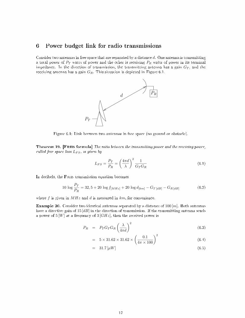
Consider two antennas in free space that are separated by a distance d. One antenna is transmittinga total power of PT watts of power and the other is receiving PR watts of power in its terminalimpedance. In the direction of transmission, the transmitting antenna has a gain GT , and thereceiving antenna has a gain GR. This situation is depicted in Figure 6.1.

dPR

PT

Figure 6.1: Link between two antennas in free space (no ground or obstacle).

Theorem 19. [Friis formula] The ratio between the transmitting power and the receiving power,called free space loss LFS, is given by

LFS =PTPR

=

(4πd

λ

)21

GTGR(6.1)

In decibels, the Friis transmission equation becomes

10 logPTPR

= 32, 5 + 20 log f[MHz] + 20 log d[km] −GT [dB] −GR [dB] (6.2)

where f is given in MHz and d is measured in km, for convenience.

Example 20. Consider two identical antennas separated by a distance of 100 [m]. Both antennashave a directive gain of 15 [dB] in the direction of transmission. If the transmitting antenna sendsa power of 5 [W ] at a frequency of 3 [GHz], then the received power is

PR = PTGTGR

(λ

4πd

)2

(6.3)

= 5× 31.62× 31.62×(

0.1

4π × 100

)2

(6.4)

= 31.7 [µW ] (6.5)

17

7 Information theory

7.1 Channel capacity

One of the central notion in communication is that of channel capacity.

Denition 21. The channel capacity is the tightest upper bound on the rate of information thatcan be reliably transmitted over a communications channel.

Theorem 22. [Shannon-Hartley] The channel capacity C (conditions for the error ratePe → 0) is given by

C [b/s] = B log2

(1 +

S

N

)(7.1)

where

• B is the channel bandwidth in Hz

• SN the signal-to-noise ratio (in watts/watts, not in dB).

7.2 On the importance of the Eb

N0ratio for digital transmissions

Assume an innite bandwidth and a Gaussian white channel, then

C = limB→∞

B log2

(1 +

S

N

)(7.2)

As

• S = EbRb (Eb is the energy of one bit and Rb = 1Tb

is the bitrate)

• N = BN0

we have

C = limB→∞

B log2

(1 +

EbRbBN0

)= limx→0

log2

(1 + xEbRbN0

)x

= log2 e lim

x→0

1

1 + xEbRbN0

EbRbN0

=

1

ln 2

EbRbN0

(7.3)

At maximum capacity: C = Rb, so that EbN0

= ln 2 ≡ −1.59 [dB] is the absolute minimum.

18

List of symbols

‖.‖ normX∗ conjugate of XB bandwidthd distancedB decibelEb bit energyfc carrier frequencyfs sampling frequencyf frequencyGR receiver antenna gaing(t) waveformH(f) transfer function or frequency responseh(t) impulse responseN0/2 power spectral density of noiseP powerPe bit error probabilityp(A) probability of Ap(t) instantaneous normalized powerPT transmit powerRb bit rateΓXX (τ) autocorrelation of a WSS random process X(t)γX(f) power spectral density of WSS random process X(t)sign(t) sign functionT time internal, period, sampling periodTb bit timet timeσ2X variance of the random variable XW bandwidthG(f) Fourier transform of g(t)x[n] discrete-time signal⊗ convolutionδ(t) unit impulse function, Diracτ time delay

References

[1] L. Couch, Digital and analog communication systems. Prentice Hall, sixth ed., 2001.

19