ANALYSIS AND IMPLEMENTATION OF THE GAS …aero-comlab.stanford.edu/Papers/jameson_int_j_num_meth_fluids_v25...international journal for numerical methods in fluids, vol. 25, 21–49

INTERNATIONAL JOURNAL FOR NUMERICAL METHODS IN FLUIDS, VOL. 25, 21±49 (1997)

ANALYSIS AND IMPLEMENTATION OF THE GAS-KINETIC

BGK SCHEME FOR COMPUTATIONAL GAS DYNAMICS

CHONGAM KIM*, KUN XU, LUIGI MARTINELLI AND ANTONY JAMESON

Department of Mechanical and Aerospace Engineering, Princeton University, Princeton, NJ 08544, U.S.A.

SUMMARY

Gas-kinetic schemes based on the BGK model are proposed as an alternative evolution model which can curesome of the limitations of current Riemann solvers. To analyse the schemes, simple advection equations arereconstructed and solved using the gas-kinetic BGK model. Results for gas-dynamic application are alsopresented. The ®nal ¯ux function derived in this model is a combination of a gas-kinetic Lax±Wendroff ¯ux ofviscous advection equations and kinetic ¯ux vector splitting. These two basic schemes are coupled through anon-linear gas evolution process and it is found that this process always satis®es the entropy condition. Withinthe framework of the LED (local extremum diminishing) principle that local maxima should not increase andlocal minima should not decrease in interpolating physical quantities, several standard limiters are adopted toobtain initial interpolations so as to get higher-order BGK schemes. Comparisons for well-known test casesindicate that the gas-kinetic BGK scheme is a promising approach in the design of numerical schemes forhyperbolic conservation laws. # 1997 by John Wiley & Sons, Ltd.

Int. J. Numer. Meth. Fluids, 25: 21±49 (1997).

No. of Figures: 27. No. of Tables: 0. No. of References: 37.

KEY WORDS: gas evolution model; gas-kinetic BGK schemes; entropy condition; gas-kinetic Lax±Wendroff ¯ux; kinetic ¯uxvector splitting; local extremum diminishing; advection equations; non-linear hyperbolic systems

1. INTRODUCTION

Over the past few decades many numerical schemes for conservation laws have been proposed to

solve gas-dynamic problems. One of the challenges is the clean capture of discontinuities such as

shock waves and contact discontinuities while maintaining high accuracy in smooth ¯ows including

expansion regions. Upstream differencing or central differencing with suitable forms of arti®cial

dissipation is generally used to compute the numerical ¯ux at a cell boundary.

The design process of current shock-capturing schemes usually consists of two stages: an

interpolation stage and a gas evolution stage based on the initial interpolated data. A clear physical

picture of a numerical scheme can be found by examining these two stages.

In the interpolation stage, gas-dynamic quantities should be estimated at a cell boundary from

discrete numerical data as accurately as possible. Remarkable progress has been made during the past

two decades in this area. FCT (¯ux-corrected transport),1,2 TVD (total variation diminishing),3

MUSCL (monotonic upwind-centred schemes for conservation laws),4,5 ENO (essentially non-

oscillation),6,7 PPM (piecewise parabolic method)8,9 and LED (local extremum diminishing)10,11

CCC 0271±2091/97/010021±29 $17.50 Received 11 January 1995

# 1997 by John Wiley & Sons, Ltd. Revised 22 July 1996

*Correspondence to C. Kim, Department of Mechanical and Aerospace Engineering, Princeton University, Princeton, NJ08544, U.S.A.

schemes are the most noticeable advances. All these schemes exclude unphysical maxima or minima

by introducing some kind of non-linear limiting process in constructing numerical data at a cell

boundary. This essentially makes each scheme ®rst-order-accurate near discontinuities. This

constraint is generally referred to as the monotonicity condition and is consistent with Godunov's

result that for a linear problem any oscillation-free scheme cannot be better than ®rst-order-accurate

across discontinuities.12

In the evolution stage a dynamic model of gas evolution based on the initial interpolated data is

applied to ®nd a numerical ¯ux at an advanced time step. The accuracy and robustness of a numerical

scheme depends on how realistically the dynamic model and interpolation principles can mimic the

evolution of a real physical ¯ow. Most of the modern high-resolution schemes use approximate or

exact Riemann solvers as the evolution model.13±15 Generally speaking, a Riemann solver assumes

constant left and right states. As observed by van Leer,16 if one uses a Riemann solver, a higher-order

scheme is obtained by introducing a higher-order interpolation subject to the monotonicity condition.

In this approach, higher-order slopes of gas-dynamic quantities are neglected after the left and right

states are obtained at a cell boundary. A gas-dynamic quantity, however, is generally changing within

a cell and this effect should be re¯ected in the gas evolution model. In this sense a Riemann solver

can be interpreted as a ®rst-order gas evolution model for a real physical ¯ow. One of the issues in the

present work is to improve this situation and to suggest a more physical gas evolution model while

utilizing current interpolation principles.

The BGK (Bhatnager±Gross±Krook) model from gas-kinetic theory describes the multidimen-

sional relaxation process of gas evolution from an initial non-equilibrium state to a ®nal equilibrium

state through particle collisions.17 From the BGK model the time-dependent particle distribution

function at a cell interface is obtained, from which the numerical ¯uxes are evaluated. In the BGK

model any kind of higher-order local slope can be essentially incorporated and upstream differencing

is achieved at the level of a particle motion. More notably, the entropy condition which is needed to

prevent unphysical discontinuities becomes naturally satis®ed. The intrinsic random motion of a gas

particle provides a new possibility to obtain a multidimensional scheme without an appropriate wave

modelling which is a crucial step in current multidimensional upwind schemes.18,19 The BGK

collisional model is different from the collisionless Boltzmann model which most Boltzmann-type

schemes have adopted.20±22 The collisionless Boltzmann model does not account for the gas

relaxation process through particle collisions. Therefore the particle distribution function in a

discontinuous region produces a large viscosity or heat conductivity due to two different half-

Maxwellian distributions constructed from the left and right states of a cell boundary. This situation

should be avoided for viscous or high-speed inviscid ¯ow computations.

Recently the successful numerical implementation of the BGK model in various ¯uid dynamic

problems has indicated the very promising behaviour of the BGK model as an alternative evolution

model for computational gas dynamics.23±26 Therefore it is necessary to characterize numerical and

physical errors in the BGK ¯ux function clearly and to ®nd the relation of the BGK ¯ux to other well-

established numerical schemes. This path is somewhat similar to the one taken in the development of

the Godunov scheme which is now recognized as an upwind scheme for gas-dynamic systems. The

previous works,23,24 however, did not address this issue. Recently it has been found that the BGK ¯ux

reduces either to the one-step Lax±Wendroff scheme or to the ®rst-order ¯ux vector splitting as the

collision time (t) of the BGK model approaches two extreme limits of zero or in®nity.25 To clarify

this interpretation, both a linear advection equation and the Burgers equation are reconstructed from

the BGK model and the algorithmic structure of the corresponding gas-kinetic schemes is analysed.

Advection equations provide simple models which represent the formation or propagation of linear

and non-linear waves, e.g. shock waves and contact discontinuities. Also, numerical results for

different initial conditions give quantitative information on the behaviour of the scheme in various

22 C. KIM ET AL.

INT. J. NUMER. METH. FLUIDS, VOL 25: 21±49 (1997) # 1997 by John Wiley & Sons, Ltd.

¯ow conditions. Each term in the ®nal BGK ¯ux function has a de®nite physical or numerical

interpretation. The ®nal BGK ¯ux has been identi®ed as a non-linear combination of the two limiting

schemes which represent the gas-kinetic Lax±Wendroff ¯ux and kinetic ¯ux vector splitting. A

simpli®ed BGK scheme which keeps important features of the original BGK scheme is also proposed.

Finally, numerical comparisons of well-known test cases for gas-dynamic systems as well as

advection equations are made to show that a scheme based on the BGK model is a promising

approach in the design of numerical schemes for hyperbolic conservation laws.

2. GAS-KINETIC RECONSTRUCTION OF ADVECTION EQUATIONS

In gas-kinetic theory it is assumed that the mascroscopic ¯uid ¯ow results from the collective motion

of a large number of molecules. The complete description of a particle motion is given by the evolution

equation of a particle distribution function f �~x; t; ~u�, where ~x is a space variable vector, t is a time

variable and ~u is a particle velocity vector in phase space. From gas-kinetic theory, every macroscopic

variable can be determined by the moments of a single scalar distribution function f �~x; t; ~u�. This

provides a uni®ed numerical approach from a scalar conservation law to systems of equations.

2.1. Analysis of the BGK model

For an advection equation with a mass variable U

Ut � a�U �Ux � 0; �1�where a�U � is a local wave speed, the relation between the macroscopic variable U and the

distribution function f is given by the moment

U �x; t� ��1ÿ1

f �x; t; u�du: �2�

The time evolution of f in three dimensions can be properly described by the Boltzmann equation

df

dt� @f@t� u

@f

@x� v

@f

@y� w

@f

@z� C� f �;

where u; v;w is a particle velocity in the x-; y-; z-direction and C� f � represents a collision integral.

The dif®culty in solving the full Boltzmann equation lies in the non-linear integral property of the

collision term C� f �. To overcome this problem, Bhatnager et al. have proposed an approximate

collisional model.17 In the one-dimensional case the evolution of f is expressed as

@f

@t� u

@f

@x� C� f � � g ÿ f

t: �3�

Equation (3) describes the gas relaxation process in which an initial distribution function f �x; t; u�approaches an equilibrium distribution function g�x; t; u� over a collision time scale t. Because we do

not have additional equations for momentum and energy, only the mass conservation constraint is

applied. From the conservation requirement that the integration of g and f with respect to the particle

velocity should represent the same macroscopic variable U, the compatibility condition is obtained:

U ��1ÿ1

f du ��1ÿ1

gdu �4�

for all x; t.

Now we may examine how the BGK model describes the macroscopic ¯ow. In a smooth region it

is reasonable to assume that the ¯ow is in a local thermodynamic equilibrium state. Hereafter an

equilibrium state means a local thermodynamic equilibrium state. Thus we may assume that the

GAS-KINETIC BGK SCHEME 23

# 1997 by John Wiley & Sons, Ltd. INT. J. NUMER. METH. FLUIDS, VOL 25: 21±49 (1997)

equilibrium distribution function is a Maxwellian distribution g � Aeÿl�uÿb�U ��2 , where l determines

the dispersion of the particle distribution function around an average macroscopic velocity, which

will be discussed more in Section 3, and b�U � is the macroscopic velocity to be determined. From

equations (2) and (4) one obtains

g�x; t; u� � lp

� �rUeÿl�uÿb�U ��2 :

If f remains in an equilibrium state with f � g, the BGK model gives

@g

@t� u

@g

@x� 0: �5�

Integrating the above equation with respect to the particle velocity in phase space (see Appendix I),

we get �1ÿ1�gt � ugx�du � hu0; git � hu; gix � Ut � �b�U �U �x � 0; �6�

where hun; gi � �1ÿ1 ungdu. As a special case of equation (1), a linear advection equation �a�U � � c�and the Burgers equation �a�U � � U � will be considered. From equation (6), b�U � � a�U � � c for a

linear advection equation and b�U � � a�U �=2 � U=2 for the Burgers equation can be used to recover

each equation in a smooth region. At the same time the Maxwellian distribution for each equation is

totally determined.

In a physically dissipative region the ¯ow is in a non-equilibrium state. The behaviour of f can be

quantitatively examined using the Chapman±Enskog expansion. The departure of f from an

equilibrium state can be obtained from equation (3) up to the ®rst order of t (see Appendix II):

f � g ÿ t�gt � ugx�: �7�Equations (3) and (4) give �1

ÿ1

@f

@t� u

@f

@x

� �du � 1

t

�1ÿ1�g ÿ f �du � 0: �8�

Substituting equation (7) into equation (8), we get�1ÿ1�gt � ugx�du � t

@

@x

�1ÿ1

u�gt � ugx�du

or

hu0; git � hu; gix � t�hu; git � hu2; gix�x: �9�By using the recurrence relation of hun; gi (see Appendix I), for a linear advection equation, equation

(9) becomes

Ut � cUx � t cUt �U

2l� c2U

� �x

� �x

� t2l

Uxx � nUxx � O�t2�; �10�

and for the Burgers equation,

Ut �U 2

2

� �x

� tU2

2

� �t

� U

2l� U 3

4

� �x

� �x

� nUxx ÿt4

U 2Ux

� �x

or

Ut �U 2

2� t

4U2Ux

� �x

� nUxx � O�t2�; �11�

24 C. KIM ET AL.


where the viscosity n is equal to the ratio of the collision time t and the equivalent temperature l. As

n! 0, equation (10) reduces to a linear advection equation. However, equation (11) does not reduce

to the Burgers equation. In this respect the Burgers equation is not proper to examine the behaviour of

the BGK model. However, equation (11) can still be analysed, at least numerically, by subtracting the

additional ¯ux �t=4�U2Ux from the BGK ¯ux. Under this modi®cation both equations (10) and (11)

become the vanishing viscosity form of the original advection equations when n! 0. This

formulation effectively circumvents the problem of differentiability near a discontinuity.27 Moreover,

the vanishing viscosity form is mathematically equivalent to the weak formulation of the advection

equations augmented with the entropy condition. Therefore it guarantees a physically correct solution

without an entropy ®x. From equations (6), (10) and (11) it is concluded that the BGK model properly

describes the essential ¯ow physics in both smooth and dissipative regions.

2.2. The gas-kinetic BGK scheme

By integrating the scalar hyperbolic conservation law

@U

@t� @h@x� 0

over a region �tj; tj � T � � �xj ÿ 12Dx; xj � 1

2Dx�, one obtains

U n�1j � U n

j �1

Dx

�tn�T

tn

�h�xjÿ1=2; t� ÿ h�xj�1=2; t��dt;

where Unj � �1=Dx� � xj�Dx=2

xjÿDx=2 U �x; tn�dx and Dx � xj�1 ÿ xj. In ®nite volume gas-kinetic schemes,

local solutions of the gas-kinetic equations are used to determine the cell interface ¯ux h�xj�1=2; t�.From gas-kinetic theory the numerical ¯ux is given by the ®rst moment of the distribution function:

h�x; t� ��1ÿ1

uf �x; t; u�du: �12�

The integral solution of the BGK equation (3) for f at the cell boundary x � xj�1=2 is28

f �xj�1=2; t; u� � 1

t

�t

0

g�x0; t0; u�eÿ�tÿt0�=tdt0 � eÿt=tf0�xj�1=2 ÿ ut� �13�

for a local constant t. Here x0 � xj�1=2 ÿ u�t ÿ t0� is a particle trajectory towards �xj�1=2; t� and f0 is an

initial distribution function at t � 0. From equations (12) and (13) one may notice that f0 and g at a

cell boundary must be estimated in order to compute a numerical ¯ux.

The initial gas distribution function f0 usually deviates from a Maxwellian. This is especially

noticeable in a discontinuous region. To re¯ect this fact in the numerical scheme, f0 is approximated

from the interpolated left and right states. In constructing f0 and g, the ®rst-order slope of space and

time variables is considered in this paper. Higher-order slopes could be incorporated in the same

manner. Without loss of generality one may assume xj�1=2 � 0. Then

f0�x; 0; u� � gl�1� alx=Dx� if x < 0;gr�1� arx=Dx� if x > 0;

��14�

where gl �p�l=p�Ule

ÿl�uÿb�Ul��2 and gr �p�l=p�Ure

ÿl�uÿb�Ur��2 are two different Maxwellians and

al and ar are related to local slopes. Note that from the results of equation (6), b�Ul� � b�Ur� � c for a

linear advection equation and b�Ul� � Ul=2 and b�Ur� � Ur=2 for the Burgers equation. Ul;Ur; al and

ar can be determined from neighbouring data by a proper interpolation principle. Recently Jameson

has proposed several numerical schemes based on the LED (local extremum diminishing) principle



that local maxima should not increase and local minima should not decrease.10,11 Applying the LED

principle to Ul;Ur; al and ar, we get

Ul � Uj � 12

L�DUj�1=2;DUjÿ1=2�; Ur � Uj�1 ÿ 12

L�DUj�1=2;DUj�3=2�;

al �1

Ul

L�DUj�1=2;DUjÿ1=2�; ar �1

Ur

L�DUj�1=2;DUj�3=2�;

where DUj�1=2 � Uj�1 ÿ Uj: L�u; v� is a limiter which will be described in Section 3. Another

distribution function g represents an equilibrium state which f approaches. Usually g can be

constructed by the Taylor expansion at x � 0; t � 0:

g � g0 1� �ax

Dx� At

� �; �15�

where g0 �p�l=p� �Ueÿl�uÿb� �U ��2 is a Maxwellian at a cell boundary and �a is related to the local slope.

The velocity �U in g0 is the average macroscopic velocity at a cell boundary and A represents the time

evolution of g0. Also, b� �U � � c for a linear advection equation and b� �U � � �U=2 for the Burgers

equation are used. By applying the compatibility condition at x � 0; t � 0; g0 can be obtained:�1ÿ1

g0du ��1ÿ1

f0du � hu0; gli� � hu0; griÿ;

where hun; giÿ � � 0

ÿ1 ungdu and hun; gi� � �10

ungdu. Thus one obtains

�U � 12�Ulerfc�ÿplb�Ul�� Urerfc�plb�Ur��;

where erfc(x) is the complementary error function. Note that the upwind biasing average of �U is

naturally obtained at the gas-kinetic level by applying the conservation requirement. The slope �a in g

is an average of the left and right slopes. Simple central differencing should be adequate, since g

represents a smooth ¯ow:

�a � 1

�UL�DUjÿ1=2;DUj�3=2� or �a � 1

�U

1

2�Uj�1 ÿ U j�:

Owing to its time-evolutionary nature, A cannot be determined from a local interpolation at t � 0.

The compatibility condition is again applied along the time axis. By substituting equations (14) and

(15) into equation (13), the distribution function at time t at a cell boundary is obtained:

f �0; t; u� � �1ÿ eÿt;t�g0 � �ÿt� �t � t�eÿt=t�u �a

Dxg0 � �t ÿ t� teÿt=t�Ag0 � eÿt=tf0�ÿut�: �16�

By using equations (15) and (16), one has

�f ÿ g��0; t; u� � ÿeÿt=tg0 � �ÿt� �t � t�eÿt=t�u �a

Dxg0 � t�ÿ1� eÿt=t�Ag0 � eÿt=tf0�ÿut�:

Now the compatibility condition is applied over the CFL time step T,�T

0

�1ÿ1� f ÿ g�dudt � 0; �17�

26 C. KIM ET AL.


which determines the time evolution term explicitly:

A � b1b� �U � �a

Dx� 1

2b2

Ulal

�Uerfc�ÿplb�Ul��b�Ul� �

eÿlb�Ul�2p�pl�

!"

�Urar

�Uerfc�plb�Ur��b�Ur� ÿ

eÿlb�Ur�2p�pl�

!#; �18�

where

b0 � T ÿ t�1ÿ eÿT=t�; b1 � �ÿT � 2tÿ �2t� T �eÿT=t�=b0; b2 � �ÿt� �t� T �eÿT=t�=b0:

Finally, the time-dependent numerical ¯ux at a cell boundary is obtained by taking the ®rst moment

of f �0; t; u� with respect to u:

h�xj�1=2; t� ��1ÿ1

uf �0; t; u�du

� a1hu; g0i � a2

�a

Dxhu2; g0i � a3Ahu; g0i � a4hu; f0i

� a1hu; g0i � a2

�a

Dxhu2; g0i � a3Ahu; g0i � a4�hu; gli� � hu; griÿ�

� a5�alhu2; gli� � arhu2; griÿ�

� a1b� �U � �U � �a

Dxa2

�U

2l� b� �U �2 �U

� �� a3Ab� �U � �U

� a4

b�Ul�2

Ulerfc�ÿplb�Ul�� eÿb�Ul�2l

2p�pl�Ul

!

� a4

b�Ur�2

Urerfc�plb�Ur�� ÿeÿb�Ur�2l

2p�pl� Ur

!

� a5

1

2b�Ul�2 �

1

2l

� �alUlerfc�ÿplb�Ul��

b�Ul�eÿlb�Ul�2

2p�pl� alUl

" #

� a5

1

2b�Ur�2 �

1

2l

� �arUrerfc�plb�Ur�� ÿ

b�Ur�eÿlb�Ur�2

2p�pl� arUr

" #; �19�

where

a1 � �1ÿ eÿt=t�; a2 � �ÿt� �t � t�eÿt=t�; a3 � �t ÿ t� teÿt=t�;a4 � eÿt=t; a5 � ÿta4:

In deriving equation (19), we have used again the recurrence relation of hun; gi� and hun; gi (see

Appendix I). The ®nal time-dependent numerical ¯ux is composed of ®ve terms.

The ®rst part �a1hu; g0i � a2��a=Dx�hu2; g0i � a3Ahu; g0i� represent a numerical ¯ux which is

dominant in a smooth ¯ow. The second part �a4�hu; gli� � hu; griÿ� � a5�alhu2; gli� � arhu2; griÿ��represents a numerical ¯ux which is dominant in a discontinuous ¯ow. These two parts are coupled in

a highly non-linear way based on the BGK gas evolution process. Though the ®nal ¯ux function looks

complicated, the analysis in the next section shows the algorithmic structure of the BGK scheme.



2.3. Analysis of the BGK scheme

To analyse the BGK scheme, the numerical ¯ux is rearranged as

h�xj�1=2; t� � h1�xj�1;2; t� � h2�xj�1=2; t�

� a1hu; g0i � a2

�a

Dxhu2; g0i � a3Ahu; g0i

� �� a4��hu; gli� ÿ talhu2; gli��hu; griÿ ÿ tarhu2; griÿ��:

Now h1�xj�1=2; t� can be rewritten as

h1�xj�1=2; t� � a1hu; g0i � a2

�a

Dxhu2; g0i � a3Ahu; g0i

� hu; g0i ÿ t�a

Dxhu2; g0i � �t ÿ t�Ahu; g0i

� �ÿ eÿt=t hu; g0i ÿ �t � t� �a

Dxhu2; g0i ÿ tAhu; g0i

� �� LW1�xj�1=2; t� ÿ eÿt=tLW2�xj�1=2; t�:

In a smooth region, from equation (14), f0�ÿut� � g0�1ÿ ��a=Dx�ut�, since the ¯ow can be assumed in

an equilibrium state. Then, from equations (16) and (15),

� f ÿ g��0; t; u� � ÿta1 u�a

Dx� A

� �g0: �20�

By applying the compatibility condition to equation (20), the time evolution term is simpli®ed to

A � ÿb� �U � �a

Dx:

Then for a linear advection equation one obtains

LW1�xj�1=2; t� � hu; g0i ÿ t�a

Dxhu2; g0i � �t ÿ t�Ahu; g0i

� c �U ÿ t�a

Dx

�U

2l� c2 �U

� �� t ÿ t� ÿc

�a

Dx

� �c �U

� c �U ÿ �a

Dx

t2l

� ��U ÿ t

�a

Dxc2 �U ; �21�

LW2�xj�1=2; t� � hu; g0i ÿ �t� t� �a

Dxhu2; g0i ÿ tAhu; g0i

� c �U ÿ �t� t� �a

Dx

�U

2l� c2 �U

� �ÿ t ÿc

�a

Dx

� �c �U

� c �U ÿ �a

Dx

t� t

2l

� ��U ÿ t

�a

Dxc2 �U : �22�

From equations (21) and (22) one may notice that LW1 and LW2 are in the same form as the numerical

¯ux of the Lax±Wendroff scheme for viscous ¯ow; that is, the numerical ¯ux in an equilibrium state

actually represents the Lax-Wendroff scheme at the gas-kinetic level. Thus h1 can be expressed as

h1�xj�1=2; t� � �1ÿ eÿt=t�L ~W �xj�1=2; t�; L ~W �xj�1=2; t� � c �U ÿ �a

Dx

~t2l

� ��U ÿ t �a

Dxc2 �U ;

28 C. KIM ET AL.


where L ~W �xj�1=2�; t� stands for a gas-kinetic Lax±Wendroff ¯ux. Here ~t is t for equation (21) and

t� t for equation (22). For the Burgers equation the same analysis leads to

L ~W �xj�1=2; t� ��U 2

2ÿ �a

Dx

~t2l

� ��U ÿ t

�a

Dx

�U3

4:

Since this is the ¯ux function for equation (11), it should be modi®ed by �t=4�U2Ux. From the

compatibility condition,

U ��1ÿ1

gdu ��1ÿ1

g0�1� At�du � �U �1� At�:

Neglecting higher-order time-dependent terms,

t4

U 2Ux �t4

�a

Dx

� ��U 3�1� At�2 � t

4

�a

Dx

� ��U 3;

so

L ~W �xj�1=2; t� ��U 2

2ÿ �a

Dx

~t2l

� ��U ÿ �t � t� �a

Dx

�U 3

4: �23�

Equation (23) has the same form as the Lax±Wendroff ¯ux. Therefore it can be considered as a gas-

kinetic variant of the Lax±Wendroff scheme.

A similar analysis can be done for h2, which can be written as

h2�xj�1=2; t� � eÿt=t��hu; gli� ÿ talhu2; gli�� hu; griÿ ÿ tarhu2; griÿ�� eÿt=t�KF� � KFÿ�;

where

KF��xj�1=2; t� � hu; gli� ÿ talhu2; gli�; �24�

KFÿ�xj�1=2; t� � hu; griÿ ÿ tarhu2; griÿ: �25�

For the sake of convenience, only a ®rst-order ¯ux with al � ar � 0 is considered. Then for a linear

advection equation one obtains

KF��xj�1=2; t� � hu; gli�

� c

2Ulerfc�ÿpc� � eÿlc2

2p�pl�Ul

� c

2Ul�1� erf �plc�� eÿlc2

2p�pl�Ul;

�26�

KFÿ�xj�1=2; t� � hu; griÿ

� c

2Ur�1ÿ erf �plc�� ÿ eÿlc2

2p�pl�Ur:

�27�



Similarly for the Burgers equation one may obtain

KF��xj�1=2; t� � hu; gli�

� U2l

41� erf

pl

Ul

2

� �� eÿlU 2

l=4

2p�pl�Ul;

�28�

KFÿ�xj�1=2; t� � hu; griÿ

� U 2r

41ÿ erf

pl

Ur

2

� �� ÿ eÿlU2

r =4

2p�pl�Ur:

�29�

Equations (26) and (27) and equations (28) and (29) are identical with kinetic ¯ux vector splitting

based on the collisionless Boltzmann equation.22 By the same procedure one may show that equations

(24) and (25) are the same as the numerical ¯ux of second-order kinetic ¯ux vector splitting.

Therefore h2 is expressed as

h2�xj�1=2; t� � eÿt=t�KF��xj�1=2; t� � KFÿ�xj�1=2; t��:Finally, the numerical ¯ux of the BGK scheme can be expressed as

h�xj�1=2; t� � h1�xj�1=2; t� � h2�xj�1=2; t�� 1ÿ eÿt=t�L ~W �xj�1=2; t� � eÿt=t�KF� � KFÿ� �30�

or

h�xj�1=2; t� � L ~W �xj�1=2; t� � eÿt=t��KF� � KFÿ� ÿ L ~W �xj�1=2; t��: �31�Thus the BGK scheme combines the GKLW (gas-kinetic Lax±Wendroff) scheme with KFVS (kinetic

¯ux vector splitting) and these two basic schemes are correlated through collision time or,

equivalently, viscosity. Some conclusions can be drawn from equations (30) and (31).

First, the two basic parts in the BGK scheme offer an intrinsic multidimensional extension. It is

known that a multidimensional form of the Lax±Wendroff scheme can be obtained for systems of

equations, although the estimation of the Jacobian matrix is expensive. In the GKLW scheme,

multidimensionality can be achieved by the interpolation of the equilibrium distribution function g.

On the other hand, multidimensional KFVS can be achieved by the interpolation of the initial non-

equilibrium distribution function f0 without resorting to wave modelling.22 The multidimensionality

of the BGK scheme can also be seen from the form of a distribution function. In a three-dimensional

advection equation the particle distribution function can be expressed as

g � Aeÿl��uÿU �2��vÿV �2��wÿW �2�;

where �u; v;w� are particle velocities and �U ;V ;W � are macroscopic velocities. Then the shape of the

distribution function is determined by the contribution of all macroscopic velocities and random

motions of particle velocities in phase space, not by the superposition of each velocity component.

Thus the ¯ux derived from the moments of the distribution function naturally considers the

multidimensionality. At this stage an initial interpolation technique which re¯ects the multi-

dimensionality should be introduced.

Second, from equation (31) one may ®nd that the BGK scheme fully utilizes the ¯ow physics in a

smooth region. Based on the BGK ¯ux, the GKLW ¯ux is modi®ed by the gas-kinetic limiter �eÿt=r�which captures the imbalance between GKLW and KFVS. This may be clearly seen if one considers

the ®rst-order ¯ux of the BGK scheme, where GKLW reduces to a central differencing type of ¯ux,

although g0 is constructured according to the upwind biasing property in the gas-kinetic level.

30 C. KIM ET AL.


Third, since the BGK scheme is identi®ed as a combination of GKLW and KFVS, one may derive

a simpli®ed BGK scheme which maintains the essential properties of the original BGK scheme. One

promising variant is

f �0; t; u� � �1ÿ eÿt=t�g0 1ÿ �a

Dxu�t � t� � At

� �� eÿt=tf0�ÿut�; �32�

where the time evolution term A can be approximated as ÿb� �U ��a=Dx. One may ®nd that the structure

for the numerical ¯ux of equation (32) is the same as equation (30), although there is a difference in

evaluating A.

3. NUMERICAL RESULTS

Since the physical thickness of a shock wave is much thinner than the grid size �Dx�, arti®cial

dissipation must be introduced to enlarge discontinuities to a scale comparable with the grid size. In

the BGK scheme the viscosity is controlled by the collision time. The collision time is de®ned as

t � t1 � t2:

Here t1 is the collision time related to the physical viscosity, which is usually very small compared

with the CFL time step, and t2 is the arti®cial dissipation to resolve discontinuities. In the case of

systems of equations such as the Euler or Navier±Stokes equations, t1 can be determined analytically

and t2 is determined by using a pressure-type switch. In the case of a scalar equation, however, there

are not enough conditions to ®x t1. Therefore t1 is ®xed to a small value compared with the CFL time

step and the following form of the collision time has been employed in all test cases:

t � 0�01� 0�5 Max�w1;w2�;

where

w1 �jUj�1 ÿ 2Uj � Ujÿ1j

jUj�1 ÿ Ujj � jUj ÿ Ujÿ1j; w2 �

jUj�2 ÿ 2Uj�1 � UjjjUj�2 ÿ Uj�1j � jUj�1 ÿ Ujj

:

Another parameter to be determined is l. As mentioned in Section 2, l controls the dispersion of a

distribution function and this is again determined analytically from macroscopic variables for systems

of equations. In all numerical test cases l is ®xed at 100. Here we again emphasize that numerical

results are not very sensitive to variation in t1 or l and l is determined analytically24 for systems of

equations. We also mention that t2 adopted in this paper is not the best choice, because we can get

much better results than presented in this paper by changing the coef®cient of t2 for each test case.

However, we have used a ®xed t2 for all test cases in order to keep the robustness of the numerical

schemes.

In the interpolation stage described in Section 2, many limiters can be used in constructing f0 or g.

The following standard limiters are employed to observe their effects and compare corresponding

current higher-order shock-capturing schemes:

(1) Minmod

L�u; v� � S�u; v�Min�u; v�;



(2) van Leer

L�u; v� � S�u; v� 2jujjvjjuj � jvj ;

(3) Superbee

L�u; v� � S�u; v�Max�Min�2juj; jvj�;Min�juj; 2jvj��;(4) a-mean with a� 2 (MUSCL)

L�u; v� � S�u; v�Minjuj � jvj

2; 2juj; 2jvj

� �;

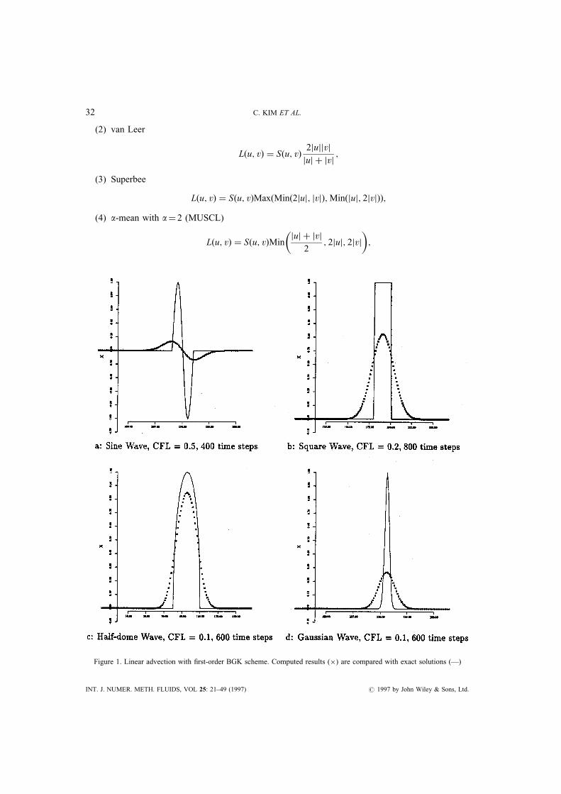
Figure 1. Linear advection with ®rst-order BGK scheme. Computed results (�) are compared with exact solutions (Ð)

32 C. KIM ET AL.


(5) second-order ENO

L�u; v� � S�u; v�Min�u; v�;

u � djÿ1=2w� 12

Djÿ1=2w; v � dj�1=2wÿ 12

Dj�1=2w;

dj�1=2w � wj�1 ÿ wj; Dj�1=2w � Min�dj�1=2wÿ djÿ1=2w; dj�3=2wÿ dj�1=2w�;where S�u; v� � 1

2�sign�u� � sign�v��. Six different schemes including a ®rst-order scheme have been

tested for advection equations. For gas-dynamic systems, several results of higher-order BGK

schemes using the MUSCL limiter are presented.

Figure 2. Linear advection with Minmod-BGK scheme. Computed results (�) are compared with exact solutions (Ð)



3.1. Advection equations

For a linear advection equation the BGK schemes are tested with four different initial pro®les: a

sine wave, a square wave, a half-dome wave and a Gaussian wave. The last three initial pro®les have

been widely used to check the behaviour of various numerical schemes1,29,30 in both smooth and

discontinuous regions. For a sine wave the CFL number is 0�5 with 400 time steps and for the other

test cases the CFL numbers and time steps are the same as in Reference 30. Figures 1±6 show the

results of each test case. In the case of the ®rst-order BGK scheme the computed results are smeared

over many cells owing to the large numerical diffusion, which is expected (Figure 1). However, the

higher-order BGK schemes not only capture discontinuities crisply but also produce excellent results

in smooth regions, except for the Minmod-BGK scheme (Figures 2±6). The effect of limiters, i.e. the

effect of interpolation techniques, is visible. The Superbee-BGK scheme produces very high peaks

Figure 3. Linear advection with van Leer-BGK scheme. Computed results (�) are compared with exact solutions (Ð)

34 C. KIM ET AL.


and sharp discontinuities but oscillates around the top of a half-dome wave (Figure 5), while the

ENO-BGK scheme shows an opposite behaviour (Figure 6) approximately. Judging from the overall

performance, the MUSCL-BGK scheme seems go give the best results (Figure 4). Comparing the

results of the BGK schemes with those of current advanced shock-capturing schemes,30 the BGK

schemes give competitive results or better accuracy for some test cases such as a half-dome wave or a

Gaussian wave.

In the case of the Burgers equation, three different initial pro®lesÐa square wave, a sine wave and

a staircase waveÐare tested. The formation and propagation of discontinuities are compared with

analytical solutions at two different times for each test case. Similar to the case of a linear advection

equation, the ®rst-order BGK scheme is rather diffusive but captures discontinuities within two or

three interior points (Figures 7±9). All the other schemes except for the Minmod-BGK scheme give

excellent results in capturing discontinuities or in smooth regions including sharp corners (Figures

Figure 4. Linear advection with MUSCL-BGK scheme. Computed results (�) are compared with exact solutions (Ð)



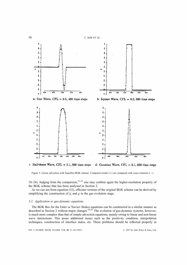
10±24). Judging from the comparison,31,32 one may con®rm again the higher-resolution property of

the BGK scheme that has been analysed in Section 2.

As we can see from equation (32), ef®cient versions of the original BGK scheme can be derived by

simplifying the construction of f0 and g in the gas evolution stage.

3.2. Application to gas-dynamic equations

The BGK ¯ux for the Euler or Navier±Stokes equations can be constructed in a similar manner as

described in Section 2 without major changes.24,25 The evolution of gas-dynamic systems, however,

is much more complex than that of simple advection equations, mainly owing to linear and non-linear

wave interactions. This poses additional issues such as the positivity condition, interpolation

techniques, construction of interface states, etc. These problems should be re¯ected properly in

Figure 5. Linear advection with Superbee-BGK scheme. Computed results (�) are compared with exact solutions (Ð)

36 C. KIM ET AL.


formulating ¯uxes to get an accurate and robust scheme. Recent work has shown that BGK schemes

possess desirable properties for such problems. In the present work we will omit this part and simply

present several results for well-known test cases. A complete description of the BGK solver for gas-

dynamic systems is given in Reference 26. Figures 25 and 26 show the results of standard shock tube

and blast wave problems. The cell distribution and CFL time step are the same as in References 7 and

9. Comparing the results with those of References 7 and 9, one observes that the BGK solver gives

results better than FCT or second-order ENO and competitive with MUSCL, fourth-order ENO or

PPM for the resolution of shock waves or contact discontinuities as well as smooth ¯ow regions.

Figure 27 shows two-dimensional examples of the unsteady Euler equations. In the shock ramp

calculations (Figure 27b) the wall jet is relatively diffuse in comparison with the PPM scheme. This is

probably due to the fact that the current BGK scheme uses a second-order initial interpolation

(MUSCL limiter) without any arti®cial sharpening technique and the solver itself yields a Navier±

Figure 6. Linear advection with ENO-BGK scheme. Computed results (�) are compared with exact solutions (Ð)



Figure 7. Burgers equation with ®rst-order BGK scheme. Computed results (�) are compared with exact solutions (Ð)



38 C. KIM ET AL.


Figure 10. Burgers equation with Minmod-BGK scheme. Computed results (�) are compared with exact solutions (Ð)





Figure 13. Burgers equation with van Leer-BGK scheme. Computed results (�) are compared with exact solutions (Ð)



40 C. KIM ET AL.


Figure 16. Burgers equation with MUSCL-BGK scheme. Computed results (�) are compared with exact solutions (Ð)





Figure 19. Burgers equation with Superbee-BGK scheme. Computed results (�) are compared with exact solutions (Ð)



42 C. KIM ET AL.


Figure 22. Burgers equation with ENO-BGK scheme. Computed results (�) are compared with exact solutions (Ð)





Stokes equation. Also, the particle diffusion is an intrinsic property in the gas-kinetic description. It is

probabaly important to study in detail the particle diffusion effect in the current BGK scheme in the

future. A rigorous comparison of computational ef®ciency is dif®cult since it depends on

programming skills among other factors. According to our experience, however, the CPU time

required by a BGK solver is comparable with that of a second-order Roe scheme with entropy ®xes.

Figure 25. Shock tube problem with MUSCL-BGK scheme. Computed results (�, 100 cells) are compared with exact solutions(Ð)

44 C. KIM ET AL.


Figure 26. Blast wave problem with MUSCL-BGK scheme. Computed results (6 , 400 cells) are compared with 800-cellcalculation (Ð)

Figure 27. Density Distributions with MUSCL-BGK scheme



4. CONCLUSIONS

In the present work the issue of errors caused by a gas evolution model as well as interpolation

principles has been addressed. The BGK ¯ux function is analysed by reconstructing advection

equations and implemented for both advection equations and gas-dynamic systems. A family of

higher-order gas-kinetic BGK schemes is derived using limiters. The resultant schemes are a

combination of a gas-kinetic Lax±Wendroff ¯ux and kinetic ¯ux vector splitting, i.e. a combination

of central differencing ¯ux and upstream differencing ¯ux. This result contrasts the BGK model with

Riemann solver, because the numerical ¯ux of a Riemann solver for advection equations reduces to

pure upwinding. The analysis presented in this work shows that the BGK model provides a more

physical gas evolution process than a Riemann solver in three important aspects.

Firstly, any higher-order slope of ¯ow variables in the interpolation stage can be readily accounted

for in constructing a time-dependent distribution function at a cell boundary. These slopes are

included during the CFL time step to obtain the ®nal numerical ¯uxes. Thus the BGK model can

describe a higher-order gas evolution process.

Secondly, the intrinsic random motion of particles is implicitly included in the form of the

distribution function. From this fact a multidimensional gas-kinetic scheme can be obtained by

introducing multidimensional interpolation of f0 and g without using macroscopic wave modelling.

Thirdly, since the BGK model essentially describes the gas evolution process of viscous ¯ow, the

gas-kinetic scheme based on the BGK model always satis®es the entropy condition.

These three properties can be fully exploited to produce a better numerical scheme.

ACKNOWLEDGEMENTS

The research in the present paper is supported by Grant URI=AFOSR F49620-93-1-0427 for all

authors. The ®rst author is also thankful for the ®nancial support provided by the Ministry of

Education in Korea. We also thank the referees for constructive comments on an earlier version of

this manuscript.

APPENDIX I: RECURRENCE RELATIONS OF MOMENTS OF

A DISTRIBUTION FUNCTION

From its construction,

hu0; gi ��1ÿ1

gdu � A

�1ÿ1

eÿl�uÿb�U ��2 du � 2Apl

�10

eÿt2

dt � 2Apl

pp

2

� �� U :

Thus we get A � p�l=p�U . Also, we get

hu; gi ��1ÿ1

gudu � Ulp

� �r �1ÿ1

eÿl�uÿb�U ��2 udu

� Ulp

� �rb�U �p

l�lperf �1�� b�U �U :

46 C. KIM ET AL.


Similarly, we may obtain

hu0; gi� ��1

0

gdu � Ulp

� �r �10

eÿl�uÿb�U ��2 du

� Ulp

� �r pp

2pl

erfc�ÿb�U �pl��

� U

2erfc�ÿb�U �pl�;

hu; gi� ��1

0

gudu � Ulp

� �r �10

eÿl�uÿb�U ��2 udu

� Ulp

� �r1

l

�1ÿb�U �pl

eÿt2 tpl� b�U �

� �dtpl

" #

� b�U �U2

erfc�ÿb�U �pl� � U

2p�pl� e

ÿb�U �2l;

hu0; giÿ � U

2erfc�b�U �pl�; hu; giÿ � b�U �U

2erfc�b�U �pl� ÿ U

2p�pl� e

ÿb�U �2l:

Now we simply apply integration by parts hun; gi:

hun; gi ��1ÿ1

gundu � Ulp

� �r �1ÿ1

eÿl�uÿb�U ��2 undu

� Ulp

� �r2l

n� 1

�1ÿ1

eÿl�uÿb�U ��2 un�2duÿ 2lb�U �n� 1

�1ÿ1

eÿl�uÿb�U ��2 un�1du

� �� 2l

n� 1hun�2; gi ÿ 2lb�U �

n� 1hun�1; gi:

Thus we get

hun�2; gi � n� 1

2lhun; gi � b�U �hun�1; gi:

By the same procedure we may obtain

hun�2; gi� � n� 1

2lhun; gi� � b�U �hun�1; gi�:

In deriving the above properties, the following relations are useful:

erf �x� � 2pp

�x

0

eÿu2

du; erfc�x� � 1ÿ erf �x� � 2pp

�1x

eÿu2

du;

erf �ÿx� � ÿerf �x�; erf �0� � 0; erf �1� � 1;

erfc�0� � 0; erfc�1� � 0:



APPENDIX II: THE CHAPMAN±ENSKOG EXPANSION OF THE BGK MODEL

The Chapman±Enskog expansion is a technique to obtain the deviation of a distribution function f

from the equilibrium state g in terms of perturbations.28,33 Consider a one-dimensional form of the

BGK model:

@f

@t� u

@f

@x� g ÿ f

t:

The variables, including distribution functions, are non-dimensionalized by

x � x

l; u � u

ur

; t � t

l=ur

; t � ttr

; f � f

fr; g � g

fr;

where l, ur, tr and fr are a characteristic length, local reference speed, local reference collision time

and local reference distribution function to make each term of order unity except for the small param-

eter E. Then the original equation is non-dimensionalized as

E@f

@t� u

@f

@x

!� g ÿ f : �33�

Now we may use a small parameter E to expand f as

f � g � Eg1 � E2g2 � . . . � P1n�0

Engn; �34�

where g0 � g. Inserting equation (34) into equation (33), we get the recurrence relation

gn � ÿ@gn�1

@t� u

@gn�1

@x

� �for n5 1. In the case n � 1 we get

f � g ÿ t@g

@t� u

@g

@x

� �: �35�

If we apply equation (35) to thermodynamic systems of equations, we get the Navier±Stokes

equations.

REFERENCES

1. J. P. Boris and D. L. Book, `Flux corrected transport, 1 SHASTA, a ¯uid transport algorithm that works', J. Comput. Phys.,11, 38 (1973).

2. S. T. Zalesak, `Fully multidimensional ¯ux-corrected transport algorithms for ¯uids', J. Comput. Phys., 31, 335 (1979).3. A. Harten, `High resolution schems for hyperbolic conservation laws', J. Comput. Phys., 49, 357 (1983).4. B. van Leer, `Towards the ultimate conservative difference scheme. II, Monotonicity and conservatin combined in a second

order scheme', J. Comput. Phys., 14, 361 (1974).5. B. van Leer, `Towards the ultimate conservative difference scheme. V. A second order sequel to Godunov's method',

J. Comput. Phys., 32, 101 (1979).6. A. Harten and S. Osher, Ùniformly high-order accurate essentially non-oscillatory schemes. I', SIAM J. Numer. Anal., 24,

279 (1987).7. A. Harten, B. Engquist, S. Osher and S. Chakravarthy, Ùniformly high-order accurate essentially non-oscillatory schemes.

III', J. Comput. Phys., 71, 231 (1987).8. P. Colella and P. Woodward, `The piecewise parabolic method(PPM) for gas-dynamical simulations', J. Comput. Phys.,

54, 174 (1984).9. P. Woodward and P. Colella, `The numerical simulation of two dimensional ¯uid ¯ow with strong shocks', J. Comput.

Phys., 54, 115 (1988).10. A. Jameson, `Positive schemes and shock modelling for compressible ¯ows', Int. j. numer. methods eng., 20, 743 (1995).

48 C. KIM ET AL.


11. A. Jameson, Ànalysis and design of numerical schemes for gas dynamics 1. Arti®cial diffusion, upwind biasing, limitersand their effect on accuracy and multigrid convergence', Int. J. Comput. Fluid Dyn., 4, 171 (1995).

12. S. K. Godunov, À difference scheme for numerical computation of discontinuous solutions of hydrodynamic equations',Math. Sborn., 47, 271 (1959).

13. R. D. Richtmyer and K. W. Morton, Difference Methods for Initial-Valued Problems, Wiley, New York, 1967.14. P. L. Roe, Àpproximate Riemann solvers, parameters vectors and difference schemes', J. Comput. Phys., 43, 357 (1981).15. A. Harten, P. D. Lax and B. van Leer, Òn upstream differencing and Godunov-type schemes for hyperbolic conservation

laws', SIAM Rev., 25, 35 (1983).16. B. van Leer, Ùpwind-difference methods for aerodynamic problems governed by the Euler equations', in Large-Scale

Computations in Fluid Mechanics, 1985.17. P. L. Bhatnagar, E. P. Gross and M. Krook, À model for collision processes in gases. I. Small amplitude processes in

charged and neutral one-component systems', Phys. Rev.l, 94, 511 (1954).18. R. Struijs, H. Deconinck, P. de Palma, P. L. Roe and K. G. Powell, `Progress on multidimensional upwind Euler solvers for

unstructured grids', AIAA paper 91-1550, 1991.19. C. L. Rumsey, B. van Leer and P. L. Roe, À multidimensional ¯ux function with applications to the Euler and Navier±

Stokes equations', J. Comput. Phys., 105, 306 (1993).20. J. C. Mandal and S. M. Deshpande, `Kinetic ¯ux vector splitting for Euler equations', Comput. Fluids, 23, 447 (1994).21. B. Perthame, `Second-order Boltzmann schemes for compressible Euler equation in one and two space dimensions', SIAM

J. Numer. Anal., 29, (1992).22. W. M. Eppard and B. Grossman, À multi-dimensional kinetic-based upwind algorithm for Euler equations', AIAA Paper

93-3303, 1993.23. K. H. Prendergast and K. Xu, `Numerical hydrodynamics from gas-kinetic theory', J. Comput. Phys., 109, 53 (1993).24. K. Xu and K. H. Prendergast, `Numerical Navier±Stokes solutions from gas-kinetic theory', J. Comput. Phys., 114, 9

(1994).25. K. Xu, L. Martinelli and A. Jameson, `Gas-kinetic ®nite volume methods, ¯ux-vector splitting and arti®cial diffusion', J.

Comput. Phys., 120, 48 (1994).26. K. Xu, C. Kim, L. Martinelli and A. Jameson, `BGK-based schemes for the simulation of compressible ¯ow', Int. J.

Comput. Fluid Dyn., 17, 213 (1996).27. R. J. Leveque, Numerical Methods for Conservation Laws, BirkhaÈuser, 1992.28. M. N. Kogan, Rare®ed Gas Dynamics, Plenum, New York, 1969.29. E. S. Oran and J. P. Boris, Numerical Simulation of Reacting Flows, Elsevier, Amsterdam, 1987.30. S. T. Zalesak, À preliminary comparison of modern shock-capturing schemes: linear advection', in Advances in Computer

Methods for Partial Differential Equations, VI, IMACS, 1987, p. 15.31. C. Hirsch, The Numerical Computation of Internal and External Flows, Vol. 2, Wiley, New York, 1990.32. H. Q. Yang and A. J. Przekwas, À comparative study of advanced shock-capturing schemes applied to the Burgers'

equation', J. Comput. Phys., 102, 139 (1992).33. W. G. Vincenti and C. H. Kurger Jr., Introduction to Physical Gas Dynamics, Wiley, New York, 1967.34. B. Einfeldt, Òn Godunov-type methods for gas dynamics', SIAM J. Numer. Anal., 25, 294 (1988).35. P. L. Roe, `Characteristic-based schemes for the Euler equations', Ann. Rev. Fluid Mech., 18, 337 (1986).36. C. W. Shu, Èf®cient implementatin of essentially non-oscillatory shock capturing schemes, II', J. Comput. Phys., 83, 32

(1989).37. P. K. Sweby, `High resolution schemes using ¯ux limiters for hyperbolic conservation laws', SIAM J. Numer. Anal., 21,

995 (1984).



Documents

ANALYSIS AND IMPLEMENTATION OF THE GAS …aero-comlab.stanford.edu/Papers/jameson_int_j_num_meth_fluids_v25...international journal for numerical methods in fluids, vol. 25, 21–49