Analysis and management of periodic review, order-up-to level

inventory systems with order crossover

ABSTRACT

In this paper we investigate the (R, S) periodic review, order-up-to level inventory control system

with stochastic demand and variable leadtimes. Variable leadtimes can lead to order crossover,

in which some orders arrive out of sequence. Most theoretical studies of order-up-to inventory

systems under variable leadtimes assume that crossovers do not occur and, in so doing,

overestimate the standard deviation of the realized leadtime distribution and prescribe policies

that can inflate inventory costs. We develop a new analytic model of the expected costs

associated with this system, making use of a novel approximation of the realized (reduced)

leadtime standard deviation resulting from order crossovers. Extensive experimentation through

simulation shows that our model closely approximates the true expected cost and can be used to

find values of R and S that provide an expected cost close to the minimum cost. Taking account

of, as opposed to ignoring, crossovers leads, on average, to substantial improvements in accuracy

and significant cost reductions. Our results are particularly useful for managers seeking to reduce

inventory costs in supply chains with variable leadtimes.

Keywords: Periodic Review Inventory Models, Leadtime Variability, Order Crossover

1. INTRODUCTION AND MOTIVATION

The past several decades have seen explosive growth in global supply chains, as an increasing

number of firms have sought to reduce costs by taking advantage of the low landed unit costs

obtained by sourcing components or finished products offshore. As Stalk (2006) has observed,

part of what has made offshore sourcing attractive are recent advances in the logistics of

containerized shipping, which have reduced port-to-port transit times across the Pacific.

However, delays in the offshore supply chain have yielded alarming increases in end-to-end

leadtimes and leadtime variability. The major causes of such delays include port congestion

(queueing delays, customs, security measures, loading and unloading times for mammoth

container carriers) and coordination of shipments with inter-modal land transit.

An often overlooked side effect of longer, more variable supply chain leadtimes is an increase in

the likelihood of order crossover and its effect on inventory costs (Robinson et al., 2001;

Riezebos, 2006). Order crossover occurs when orders arrive out of sequence, such as when an

order N, placed later than another order M, arrives prior to order M. The occurrence of crossovers

is not restricted to long, global supply chains. As Srinivasan et al. (2011) have noted, crossovers

can occur in practice for a variety of reasons, not necessarily related to supply chain length. For

example, the adoption of lean, JIT systems brings a reduction in batch sizes, leading to more

frequent ordering that increases the likelihood of crossover. Other contributing factors to

crossovers include shipment consolidation, variable transportation times due to the use of

multiple suppliers, and rescheduling of orders due to production constraints.

In this paper we examine the effect of order crossover on the (R, S) periodic review, order-up-to

level inventory control system under stochastic demand and/or variable leadtimes. As Srinivasan

et al. (2011) have observed, order crossover poses theoretical difficulties in the prescription of

optimal policies for (R,S) inventory systems with variable leadtimes—that is, an (R,S) policy is,

in general, not optimal under these conditions. However, as the (R,S) inventory system is

commonly used in supply chains to facilitate the coordination of product flows, and since

theoretical approaches to this problem have either ignored the effect of crossovers or have

contrived model constructions that prohibit crossovers in order to preserve model optimality, it is

important to explore how order crossover affects the costs associated with the (R,S) system in

practice, especially since Robinson et al. (2001) found that the effect of crossovers on inventory

costs can be large even in those cases in which crossover is relatively unlikely. We develop a

new analytic model of the expected costs for an (R, S) system that includes both stochastic

demand and leadtimes (Gross and Soriano, 1969). Alternate systems for handling stochastic

demand and leadtimes are addressed by Bagchi et al., 1986; Kumar and Arora, 1992; Song et al.,

2000; and Ayanso et al., 2006. Our model incorporates a novel approach to estimate the realized

(reduced) leadtime standard deviation resulting from order crossovers, and we demonstrate

through extensive simulation experiments that our model closely approximates expected cost

under a wide range of cost, demand, and leadtime parameter values. The model can be used

relatively easily to select an appropriate (R, S) policy, and by taking advantage of the crossover

effect, we obtain policies that tend to have lower values of R and S as well as lower expected cost

than the best (R, S) policy chosen using models that ignore crossover. Under situations in which

crossovers are unlikely, our policies are identical to the traditional (R, S) policy.

Although crossovers may be problematic in theory, in practice they are surprisingly beneficial.

For a given leadtime distribution, the occurrence of crossovers leads to an effective, or realized,

leadtime distribution with a smaller standard deviation (Hayya et al., 2011). Conventional (R, S)

policies that ignore crossovers will overestimate the realized leadtime standard deviation and

thereby incur cost penalties due to excessive inventory levels and safety stocks. Our modeling

approach exploits the effect of crossovers to develop least-cost or lower-cost (R, S) policies.

In the next section we discuss our approximation of the cost effect of order crossover and present

our analytic model of expected cost. In Section 3 we use our model under a variety of cost

parameter values and demand and leadtime distribution conditions to find values of (R, S) that

minimize the approximated expected cost. Simulation experiments demonstrate how well our

model approximates the true expected cost and the improvement in cost performance compared

with that obtained using (R, S) models ignoring crossover. In Section 4 we show that one of the

key assumptions of the model (namely independent leadtimes) can be relaxed. We conclude with

a brief summary; technical details are given in the Appendix.

2. MODEL DEVELOPMENT

We consider the procuring of a single item with unit variable cost, c (see Table 1 for notation).

Every R days the inventory is reviewed, and an order is placed (with a fixed cost A) to raise the

inventory position to S. This order is available L days later, where the leadtime L is a random

variable, independent of the order size and independent of other leadtimes. (The latter

assumption is relaxed later in the paper.) The total relevant costs associated with the system are

the sum of the inventory holding costs, the fixed costs of replenishments, and the shortage costs.

To determine appropriate choices for the review period R and order-up-to level S, we develop an

analytic expression for the expected total cost. (We treat R as a decision variable, but our

approach can easily be modified to handle a pre-specified R value that could be determined

based on transportation economies, manufacturing schedules or multi-item order coordination

requirements.) We comment on our modeling assumptions and consider their validity

subsequently, but first we address the important issue of order crossovers caused by the random

leadtimes. Incidentally, Hayya and Harrison (2010) incorporate crossovers for continuous

review, order point/order quantity models under deterministic demand and exponentially

distributed leadtimes. As well, for the case of discrete demand and leadtime distributions

Srinivasan et al. (2011) use simulation search to find the best value of S. (In their study, R is

assumed to be given.)

2.1 Crossovers Caused by Random Leadtimes

As crossovers can have an important effect, particularly on expected shortage costs, various

methods for dealing with them have been proposed, including stochastic dynamic programming

(Riezebos and Gaalman, 2009) and setting S based on the distribution of the shortfall (the gap at

the start of a period between the inventory position and S) – see Bradley and Robinson (2005)

and Robinson and Bradley (2008).

We account for order crossover through the use of an effective leadtime, a concept introduced by

Hayya et al. (2008). Consider a sequence of consecutive orders numbered 1, 2, 3, etc., placed at

times t1, t2, t3, etc. Let the chronologically-ordered arrival times be denoted by 1 2 3, , , etc.

Note that, due to possible crossovers, i does not necessarily represent the arrival time of order i.

Thus it is the effective leadtimes, defined as 1 1 1 2 2 2, ,..., ,... ,i i it t t L L L and not the

original Ls, which determine costs. Moreover, although ,L

L L can be much smaller than

L , as shown in Hayya et al. (2008) using order statistics and in Bradley and Robinson (2005)

by means of an analytic result through an upper bound on the number of outstanding orders.

In order to incorporate effective leadtimes into our model, we first used simulation to estimate

L for various values of R under the assumption of independent Gamma-distributed leadtimes.

(We discuss the use of the Gamma leadtime distribution in Section 3.1 below.) We then fit the

analytic relationship

1.08981 0.8758 expL

L

R

L (1)

to the results (see Figure 1) using a minimax criterion. This expression has the appealing

limiting behavior of 1L L as LR , i.e., there is no adjustment to variability when

crossovers become negligible. Moreover, the expression is more parsimonious than the

piecewise linear function of Hayya et al. (2009), and it provides a very close fit for broader

parameter ranges. (Although (1) was developed using Gamma-distributed leadtimes, the same

structural form with only slightly different coefficient values also holds for Lognormal and

Weibull leadtime distributions.)

Note that the presence of crossovers implies that an (R, S) policy is not an optimal policy in that

an ordering decision at the beginning of a period should, in principle, take account of the timing

of each of the outstanding orders. Srinivasan et al. (2011) investigate such policies through the

use of Markov decision processes and simulation search. In this paper we stay with the widely

used and much more easily implemented (R, S) policy.

2.2 Cost Expression and Normalization

Let D represent the daily demand with mean D and standard deviation D . The effective

leadtime L , which replaces L throughout the analytic model, has mean L and standard

deviation L . If X signifies the demand during the key “protection interval” R L , X is then

the random sum of R L daily random demands. Assuming that D and L are independent, the

mean of X, X , and its standard deviation X are, respectively (see Silver et al. (1998)),

( ) DR L and 2 2 2( ) D DR L L . Similarly let Y represent the demand during the

effective leadtime. Then Y and Y are given, respectively, by D L and 2 2 2

D D L L .

If a replenishment with fixed cost A takes place at each review, and full backordering occurs

with a charge of Bc per unit short, then the expected total cost per day is approximately

0

0

0 0 0 0 0 0

0 | 0 0 0 0

0

( , ) ( ) ( ) ( ) ( )2

( ) ( ) ( )

D X Y

X W t

S S

R

S

R A BcEC R S rc X S f X dX Y S f Y dY

R R

rcrc S W S f W dW dt f d

R

L

L

LL L

(2)

where r is the inventory holding charge ($/$/day), 0( )Xf X , 0( )Yf Y and 0( )fL L are the probability

density functions of X, Y, and L , and | 0W tf W is the probability density function of the demand

in a period of length t. The first two terms on the right hand side of (2) are the cycle stock

holding cost and the fixed cost of replenishments, and the expression in the first large brackets is

the expected units short per cycle (de Kok, 1990; Hadley and Whitin, 1963). On the second line

the first term is the safety stock holding cost, and the last expression adjusts for the expected

level of backorders at a random point in time, based on Hadley and Whitin (1963), which we

have extended to include variable leadtimes.

Here are reasons why (2) is not an exact expression for the expected cost. In general, the

distribution 0( )fL L is not known exactly, hence must be approximated by a convenient analytic

form, which will be discussed below. Furthermore, if orders cross, not just the arrival times but

also the order quantities will cross, and thus the arriving order size may not match the desired

order size. We return to this latter issue in Section 3.2.

In some circumstances the purchaser may have to pay for pipeline inventory. For example, if

payment terms are Free-On-Board, there will be an additional expected cost component of

.DrcL This term is independent of R and S and so does not affect their selection, but it will

affect total inventory costs.

We express the order-up-to level as follows:

X XS k (3)

where, as usual, k is a safety factor, and define the ratio between shortage and holding costs as

rB / (4)

In addition we define

cr

Aw

D

2 (5)

where w is the deterministic equivalent EOQ, expressed in days of demand, also known as the

Wilson number.

Equation (2) can be normalized to reduce the number of parameters by dividing by the cost of

holding one day’s worth of demand in inventory for a period of one day, i.e., D cr . We also

substitute (3), (4) and (5) to obtain the Normalized Expected Total Cost (NEC) as

0 0 0

0

0

|

2

0 0 0 0 0 0

1( ( )) ( )

( , )( , )

2 2

[ ( )] ( ) [ ( )] ( )

X X X X

X X

X X W

D

D

X X X X X YD k k

R

Xt

kD

W k f W dW dtR

EC R S R wNEC R k

cr R

X k f X dX Y k f Y dYR

k

L

L0 0

0

( )f d

L L L

(6)

which holds for any distributions of X , Y, and |W t . The units for NEC are “days holding

cost”— units that managers, who typically refer to inventory costs over time periods, would use.

Empirical studies such as Strijbosch et al. (2002) have found that the Gamma distribution

provides a good fit for total demand over a specified period of time. While one study (Tyworth

and O'Neill, 1997) has concluded that employing a Normal approximation for leadtime demand

is fairly robust, we find that this is not the case for demand distributions in supply chains with

high levels of leadtime uncertainty. These distributions tend to be asymmetric over non-negative

values, with a long right-hand tail. Due to the flexibility provided by its shape parameter, the

Gamma family of distributions provides significantly better fits than the Normal; in particular,

the latter can result in significant probabilities of negative values of demand for small values of

µL/σL (Chopra et al., 2004; Tadikamalla, 1984).

For Gamma distributed X and Y it is shown in the Appendix that

0

0

0 0

2

2 2 2 2 2 2

0 0 0|0

1( )

,

( ( )) ( )

( , )2 2

( ) ( , )

X X

sG

D

D DsG

R

X X Wk

t f d

G kR

W k f W dW dtR

R wNEC R k

R

R v v k G k v vR

L

L L L L L L

L

LL L

(7)

where vD and ( / )v L L L are the coefficients of variation of the (daily) demand and the

effective leadtime,

22

2 2 2 2

( )

( )

X

X D

R

R v v

L

L L L and

22

2 2 2 2

Y

Y Dv v

L

L L L are the shape

parameters of the X and Y distributions, and 2 2 2 2( )

X

X D D D

R

R v v

L

L L L and

2 2 2

1Y

Y D D Dv v

L L are their scale parameters. Note that L is found through the use of

(1). ( , )sGG u is the standardized linear loss function, as defined in terms of incomplete Gamma

functions by (A2) in the Appendix. We note that expression (7) would somewhat simplify if

demands and leadtimes were assumed to be Normally distributed, but then its cost performance

would increasingly deteriorate with uncertainty.

For the special case in which the leadtime is Gamma distributed but demand per period is

constant, that is, when vD = 0, X follows a shifted Gamma distribution (with minimum value

µDR), and there is considerable simplification of the NEC expression. Details are available, on

request, from the first author.

While the first two terms of (7) are convex in R, the others may not be (Silver and Robb, 2008).

Indeed, even in the case of deterministic leadtimes, Liu and Song (2012) have shown that the

average cost function is not jointly convex in R and S. As we are unable to prove convexity of

NEC for Gamma-distributed X , Y, and |W t , we conduct a two-dimensional grid search to find

the best (in terms of minimizing NEC) combination of reorder period and order-up-to level

(denoted by R* and S*, respectively). Note that it is straightforward to evaluate (7) using, e.g.,

Mathematica®, numerically integrating the last component. (A copy of the Mathematica code is

available from the first author.)

2.3 A Simple Heuristic

We also evaluated the performance of a heuristic to select S, given R, that does not require

integration. As shown in the Appendix, by neglecting two terms in (7) – the second Gamma

term, which is likely to be considerably smaller than the first one, and the backorder term, which

is usually relatively small – we can obtain a closed-form approximation for the value of k, and

hence S, for a given value of R as follows:

11, ,ap

sG

Rk p

(8)

where 1 ,1sGp q

is the qth quantile of the standard Gamma distribution with parameter α

(Fortuin, 1980). Note that kap

depends upon the shape parameter but not upon the scale

parameter of the Gamma distribution of X, and depends only upon R, μL, vL, and vD and not

upon μD (see (A1) in the Appendix).

For given R, we evaluate kap

from (8) and then use it to calculate S(R) from (3). The heuristic’s

performance is evaluated in Section 3.3.

3. SIMULATION EXPERIMENTS AND RESULTS

In this section we present the results of simulation experiments used to examine the performance

of both our analytic model and the simple heuristic. We first discuss the simulation model and

the parameter set chosen for the experiments. After presenting the results of the experiments, we

discuss their implications concerning the importance of taking crossovers into account through

the incorporation of the effective leadtime.

3.1 Simulation Model and Selection of Parameter Values for Experiments

Simulation was employed in order to provide an estimate of the true normalized expected daily

cost of operating at a given choice of (R, S). The simulation model was developed in ARENA

(Version 10, Rockwell Software, Inc.). In the simulation model, orders arrive at the beginning of

the day, after which an order is placed if needed; the day’s demand then occurs.

Based on our experiences with industrial data sets and on the literature, in the simulations we

modeled both daily demand and the leadtime with Gamma distributions (e.g., Fortuin 1980;

Cachon 1999; Strijbosch et al. 2002). Note that this does not satisfy the analytic model’s

assumption that X and Y have Gamma distributions, since in general a random sum of Gamma

variables is not Gamma distributed. As we observed that high-variance Gamma random variates

generated by ARENA were inaccurate, variates were instead generated in Mathematica and input

to ARENA to drive the simulation. (All results are available from the first author upon request.)

To test the analytic model, we first employed a grid search in Mathematica to find values of (R*,

S*) and the resulting NEC for 243 cases determined by setting each of five parameters (w, ρ, vD,

μL, and vL) at one of three values. (Along with Gross and Soriano (1969), we found that the

mean demand had very limited impact on NEC, and so μD was set to 100 for all experiments.)

For the grid search we set the minimum allowable safety factor to zero (see Silver et al. 1998 and

Teunter et al. 2010, who also make this assumption), since in a practical context many managers

would be reluctant to have negative safety stock. (This constraint turned out to be binding in

only a few cases.) The CPU time required for the grid search will depend upon the range of R

and k values considered and the fineness of the grid. Searching over all integer values of R from

1 to 200 and from k = 0 to 6 in increments of 0.1 required under two minutes of CPU time per

case on a 2.40GHz processor.

Concerning the use of (μL, vL) as leadtime parameters rather than (μL, σL), our observations of

leadtime data in contexts including domestic supply and international shipping (Fang et al.,

2012) suggest that the relationship between σL and μL is approximately linear, so that vL is

roughly constant. Thus one need only vary μL to reflect the realistic impact of changing the

average leadtime. Similarly, a smaller value of vL reflects the impact of uncertainty reduction,

e.g., through switching to a more reliable supplier or by process improvement that reduces σL

while holding μL constant. Again, to reflect a wide variety of industrial sourcing environments,

we consider μL values of 4, 25, and 100 days and vL values of 0, 0.25, and 0.5, the latter as in van

der Heijden and de Kok (1998).

The remaining parameter settings were determined by extending the range beyond what we

observed in industrial data sets in order to “stress test” the model under extreme conditions of ρ,

w, and vD. We set w to 1, 20, and 100 days and used ρ values of 100, 500, and 2000. The lowest

value of ρ represents the situation of substantial depreciation (i.e., a high value of r), e.g.,

computer hardware (Kapuscinski et al., 2004), whereas the highest value of ρ reflects

circumstances of very high loss of goodwill (i.e., a high value of B). The coefficient of variation

of (daily) demand, vD, was set to 0, 2.5, and 5, comparable to empirical observations (Silver and

Robb, 2008).

3.2 Analytic Model Performance

We present results on two aspects of model performance: first, how closely our model

approximates the expected cost at (R*, S*), and second, how well this expected cost compares

with the expected cost of the globally minimum cost selection of R and S.

Comparison of the analytic model cost to the expected cost at the analytic model solution

For each of the 243 cases, after completing the grid search on (7) to find (R*, S*) and the

corresponding approximate NEC, we used simulation to estimate the actual expected cost at (R*,

S*), using a warm-up period of 1 million days and a run of 25 million days. Each case required

less than 10 minutes to run. (The average 95% confidence interval half-width on expected cost

was 0.2%, with a maximum value of 0.66 %.)

Table 2 presents a summary of the accuracy of the analytic model cost, averaged within each

parameter value. The absolute percentage differences between the analytic and simulated values

of NEC average just 0.9%. Moreover, 90% of the 243 cases show cost differences of no greater

than 2%, indicating that the analytic model is quite accurate most of the time.

The 18 largest absolute percentage errors (with a maximum error of 21.3%) all occurred for

0Dv , and the seven largest of these occur when w=1 (leading to R=1). In addition, three of the

four largest absolute percentage errors are for μL=100 and vL=0.5 (i.e., L =50). This combination

of parameters—implying no variation in demand, 100 orders outstanding on average, and an

enormous number of crossovers—would be highly unlikely in practice.

Most of the remaining errors in NEC stem from inaccuracies in estimating the effects of order

crossover on the expected units short. The larger errors tend to occur for very small values of

/ LR , where the discrepancy between the fitted regression and the simulated values of L is

greatest (see Figure 1). If necessary, one could develop a more accurate regression in this

region. We also observed from a histogram of the effective leadtimes that, as the number of

crossovers gets very large (again for very low / LR ), the distribution more closely fits a

Normal than a Gamma. An intuitive explanation is that the total demand, X, is the sum of R plus

L Gamma variables, where L is random. For R large relative to L , X is approximately the sum

of R Gamma variables and thus is approximately Gamma distributed. However, when R is small

relative to L , X is predominantly a random sum of Gamma variates which, as mentioned earlier,

is not well fitted by a Gamma distribution. Thus, we examined the impact of using the simulated

L (as a surrogate of a more accurate regression) and a Normal distribution for each of X and Y

where / 0.2LR . This drastically reduces the largest absolute percentage errors.

Variability in order sizes could, in principle, increase errors in the model’s estimate of the

expected units short due to order and arrival sizes not matching (as orders cross), especially in

cases of higher vD and lower R. However, an extensive, supplementary numerical investigation

identified that, at least for the range of parameters considered here, shortage costs are primarily

influenced by when orders arrive and not by the magnitude of the individual orders received.

We investigated two other possible sources of inaccuracy in estimating the expected units short.

In the simulation, generated leadtimes are rounded to (positive) integer days. Since for vD=0 and

an effective leadtime0L , the total demand X in

0RL is 0D R L , the generated total

demand has a discrete distribution with values of 1 , 2D DR R , etc., whereas the

analytic model assumes a continuous Gamma distribution. However, we found that

incorporation of a discrete leadtime in the model actually caused a slight deterioration in

performance.

Finally, another source of discrepancy was that in the simulation the generated daily demand is

rounded to the nearest integer, including zero, making it possible that no demand occurs in the

entire review cycle and hence no replenishment takes place. We fine-tuned the analytic model to

correct for this by multiplying the order cost term (the first term in (7)) by

1 Prob 0.5 ,R

D which is readily computed a priori for a given demand distribution and

value of R. However, this adjustment proved unimportant except in cases with highly variable

demand and w=1 (implying an R of 1 or 2), for which it still amounted to less than 0.9% of NEC.

Comparison of the expected cost at the analytic model solution to that of the best solution

It is also of interest to compare the cost performance of (R*, S*) to that of the best (R, S) pair

found by two-dimensional grid search using the simulation model, since, due to the analytic

model’s approximation of the true cost surface, the cost of operating at (R*, S*) may differ from

that of the optimal (R, S). The first column of Table 3 presents the percentage cost penalty

between the simulated cost at (R*, S*) and the minimum cost solution found with the simulation

grid search, averaged by parameter value. The average percentage cost penalty is only 0.5%, and

all but 9 cases (out of the 243) have percentage cost penalties of no more than 2%. Similar to the

results on the errors due to the approximation of NEC, the percentage cost penalties are highest

when 0,Dv and three of the four largest absolute percentage errors are for μL=100 and vL=0.5.

In summary, these results provide additional evidence that the analytic model is highly effective.

3.3 The Performance of the Simple Heuristic

The additional cost penalty incurred by using the heuristic described in Section 2.3, rather than

the analytic model, is summarized in the second column of Table 3. The heuristic performs quite

well, with an average percentage cost penalty of only 2.2%.

However, we observed that the penalty can be high (up to 34%) for cases in which w =1 (which

generally implies small, frequent orders—that is, small R values). In this case the difference

between the two Gamma terms in (7) is small, and the heuristic (which ignores the second

Gamma term) tends to overstate expected penalty costs and thus mis-specify the (R, S) pair.

3.4 The Importance of Incorporating Effective Leadtimes

We performed additional tests to evaluate the importance of using the effective leadtime as a

means of accounting for crossovers. It is clear from Figure 1 that in cases where / LR exceeds

10 or so, the values of L and L are essentially equal because the likelihood of crossovers is

negligible, hence the effective leadtime concept is irrelevant. For the 125 (out of 243) cases

where there was a nontrivial difference between L and L , we replaced L

in (7) with the

original leadtime standard deviation L (i.e., ignoring crossovers) and used a grid search to find

R and S. Not taking account of crossovers when L < L leads to higher values of both R and S.

For a given value of R, using L , instead of L , results in a larger value of S. The increase in R

results from the associated effect in the ρ/R factor in the shortage term of (7). Looking at this

from the opposite perspective, when we properly take account of crossovers we see that R is

decreased which, in turn, leads to even more crossovers, which is beneficial from a cost

standpoint.

We then evaluated each solution by simulation. The cost at the (R, S) pair found by using (7)

(with L ) was, on average, 11% lower than the cost at the (R, S) pair found with L . In 30

cases the cost improvement exceeded 10%, and the largest decrease observed was 82%. Using

the effective leadtime produced the greatest percentage benefit in cases with small w (which

implies low R, i.e., frequent orders), highly-variable leadtimes (i.e., high L , which is the

product of µL and vL), and low demand variation. Table 4 displays the relationship between w,

probability of crossover, and percentage cost improvement from using the effective leadtime.

When w = 1, we observe the highest average probability of crossover (low values of / LR ) and

also the greatest improvement from using the effective leadtime. The likelihood of crossover

and potential for improvement each decrease with increasing values of w (i.e., larger values of

/ LR ).

Furthermore, as there are two sources of variability present, namely in D and L, reducing the

uncertainty in L by using L instead of L is most beneficial from a percentage cost reduction

standpoint when vD is low, because we are then reducing the primary source of uncertainty.

However, note that absolute costs increase with vD; hence, even if the percentage cost reduction

is lower, the absolute cost reduction can still be appreciable.

In additional experimentation with / LR ranging between 0.2 and 0.5, w = 20, and moderate

values of vD = 0.5 to 1.5, substantial cost improvements of 12% to 43% were obtained. In

summary, the use of effective leadtimes to incorporate crossovers can lead to major

improvements in the accuracy of the estimated inventory cost and, with appropriately modified

values of R and S, to significant cost reductions.

4. EXTENSION TO AUTOCORRELATED LEADTIMES

To this point we have assumed independent leadtimes, partly because it facilitated examination

of the effects of changing a number of parameter values ( , , ,D L Lv v w , and ). In addition,

independent leadtimes have been implicitly assumed in much of the literature on order-up-to

policies and in applications of these policies to practical operating systems. However, we now

show that our general approach can be easily adapted to handle leadtimes that display

autocorrelation, which in practice may be more prevalent than independent leadtimes. In

particular, positive autocorrelation would indicate that a factor (such as supplier slowdowns, port

congestion, or natural or other disasters) has a similar effect on consecutive leadtimes.

Fortunately, even with autocorrelated Ls the concept of effective leadtimes is still applicable, and

the only modification required is how L is determined. Given a value of the autocorrelation

coefficient, we can use the procedure described in Section 2.1, but simulating serially correlated

Gamma-distributed leadtimes (Cario and Nelson, 1996) rather than independent leadtimes, to

obtain an analytic relationship for / L L that replaces expression (1). We did this using an

autocorrelation coefficient of 0.67, based upon data from an industrial application. The following

form provided an excellent fit to the empirically generated L values:

2.9531 0.8078 expL

L

R

L . (9)

It can easily be shown that the right-hand side of (9) is greater than that of (1) for all values of

/ LR , suggesting that, as expected, positive autocorrelation reduces order crossover.

We explored the performance of our approach by again setting 100D and, based upon the

industrial source of the autocorrelated leadtime data, using 1.75, 36, 0.2,D L Lv v and

100 ; although in the specific case w was approximately 25 days, we modified this parameter

value to 1w in order to obtain a nontrivial probability of order crossover. We then performed a

grid search to identify (R*, S*) under each of three experimental conditions: (a) taking neither

the crossovers nor the correlation into account, but simply using the original L ; (b) taking the

crossovers but not the correlation into account, by using L as derived from the regression

relationship given in (1); and (c) taking both the crossovers and the correlation into account, by

using L derived from the relationship in (9). We then ran a simulation at each (R*, S*) using

Gamma leadtimes with an autocorrelation of 0.67 and also ran a simulation search to find the

lowest possible cost.

We found that the percentage cost penalties due to using the analytic solutions rather than the

best solution were (a) 2.5%, (b) 0.10%, and (c) 0.03%. Thus even using the effective leadtime

relationship based on independent leadtimes provided a substantial improvement in cost

performance, and the introduction of the autocorrelation-based relationship further improved

performance. We also found, as expected, that the autocorrelation reduced the likelihood of

crossovers—from 42% in the independent-leadtimes case to 40%. However, the best simulated

expected cost per period for the autocorrelated case was only 3% higher than that of the

independent case. In summary, it is straightforward to extend the analytic model (with its

associated benefits) to the case of autocorrelated leadtimes.

5. SUMMARY AND CONCLUSIONS

In this paper we have developed a new analytic model of the inventory-related costs of the (R, S)

inventory control system, which is commonly used in supply chains. The model incorporates

Gamma-distributed demand and leadtimes and includes an approximation to account for the

impact of order crossovers, which can occur with variable leadtimes. Because crossovers tend to

reduce the variability of the realized leadtime distribution, we capture this effect in our model by

replacing the given leadtime standard deviation with an effective leadtime standard deviation that

adjusts for the likelihood of crossover. We found that, using the effective leadtime distribution,

the analytic model performed very well under a variety of conditions that encompass most

supply chain environments.

Moreover, we showed that taking account of order crossovers by using the effective leadtime

provides much more accurate estimates of the inventory cost than using (R, S) inventory models

that ignore crossovers. A traditional (R, S) inventory model that ignores crossovers

overestimates leadtime variability and therefore prescribes policies with higher safety stock

levels than needed, inflating costs. Our model exploits the crossover effect and yields (R, S)

policies with lower R and S values appropriate for the lower realized level of uncertainty; these

policies have lower average inventory levels and lower expected total cost. Under conditions in

which crossovers are highly unlikely (that is, when L and L are essentially equal), our model

applies without modification and provides results identical to those obtained using a traditional

(R, S) model. The model is relatively easy to implement, requiring the calculation of expression

(7) for each potential value of R and k; this is straightforward to do in Mathematica or a similar

package. Note that (7) incorporates the analytic relationship between L and L that is given in

(1); as this expression holds for any Gamma-distributed leadtime, it is not necessary to

recalculate the expression’s coefficients. We found that the same structural form holds for

Lognormal or Weibull-distributed leadtimes but with slight changes in the values of the

coefficients.

This work has important practical implications for managers of supply chains. Developing

trends suggest that supply chains will experience order crossover with increasing frequency. The

popularity of JIT-induced shorter order cycles and smaller batch sizes and the growing length,

complexity, and uncertainty in global supply chains are factors that combine to increase leadtime

variability and raise the likelihood of order crossovers. For these environments we provide

managers with an inventory model that captures the beneficial effects of crossovers and that

yields policies which reduce their inventory costs. In addition, the model is easily adapted to

incorporate autocorrelated leadtimes and also applies in a multi-product environment.

REFERENCES

Ayanso, A., M. Diaby, and S.K. Nair. 2006. Inventory rationing via drop-shipping in Internet

retailing: A sensitivity analysis. European Journal of Operational Research 171:135-152.

Bagchi, U., J. C. Hayya, and C.-H. Chu. 1986. The effect of lead-time variability: The case of

independent demand. Journal of Operations Management 6 (2): 159-177.

Bradley, J. R., and L. W. Robinson. 2005. Improved base-stock approximations for independent

stochastic lead times with order crossover. Manufacturing & Service Operations

Management 7 (4):319-329.

Cachon, G. P. 1999. Managing supply chain demand variability with scheduled ordering

policies. Management Science 45: 843-856.

Cario, M.C., and B.L. Nelson. 1996. Autoregressive to anything: Time-series input processes

for simulation. Operations Research Letters 19: 51-58.

Chopra, S., G. Reinhardt, and M. Dada. 2004. The effect of lead time uncertainty on safety

stocks. Decision Sciences 35 (1):1-24.

de Kok, A. G. 1990. Hierarchical production planning for consumer goods. European Journal of

Operational Research 45:55-69.

Fang, X., C. Zhang, D.J. Robb, and J.D. Blackburn. 2012 (In press). Decision support for lead

time and demand variability reduction. OMEGA -- The International Journal of

Management Science.

Fortuin, L. 1980. Five popular probability density functions: A comparison in the field of stock-

control models. Journal of the Operational Research Society 31 (10):937-942.

Gross, D., and A. Soriano. 1969. The effect of reducing leadtime on inventory levels - simulation

analysis. Management Science 16 (2):B61-B76.

Hadley, G., and T. M. Whitin. 1963. Analysis of Inventory Systems. 1st ed. Englewood Cliffs,

NJ: Prentice-Hall.

Hayya, J. C., U. Bagchi, J. G. Kim, and D. Sun. 2008. On static stochastic order crossover.

International Journal of Production Economics 114 (1):404-413.

Hayya, J. C., and T. P. Harrison. 2010. A mirror-image lead time inventory model. International

Journal of Production Research 48 (15): 4483-4499.

Hayya, J. C., T. P. Harrison, and D. C. Chatfield. 2009. A solution for the intractable inventory

model when both demand and lead time are stochastic. International Journal of

Production Economics 122 (2):595-605.

Hayya, J. C., T. P. Harrison, and X. J. He. 2011. The impact of stochastic lead time reduction on

inventory cost under order crossover. European Journal of Operational Research 211:

274-281.

Kapuscinski, R., R.Q. Zhang, P. Carbonneau, R. Moore, and B. Reeves. 2004. Inventory

decisions in Dell's supply chain. Interfaces 34 (3):191-205.

Kumar, S., and S. Arora. 1992. Effects of inventory miscount and non-inclusion of lead time

variability on inventory system performance. IIE Transactions 24 (2):96-103.

Liu, F., and J.-S. Song. 2012. Good and bad news about the (S,T) policy. Manufacturing &

Service Operations Management 14(1): 42-49.

McCullough, B. D., and B. Wilson. 2005. On the accuracy of statistical procedures in Microsoft

Excel 2003. Computational Statistics & Data Analysis 49: 1244-1252.

Riezebos, J. 2006. Inventory order crossovers. International Journal of Production Economics

104:666-675.

Riezebos, J., and G. J. C. Gaalman. 2009. A single-item inventory model for expected inventory

order crossovers. International Journal of Production Economics 121 (2):601-609.

Robinson, L.W., and J.R. Bradley. 2008. Further improvements on base-stock approximations

for independent stochastic lead times with order crossover. Manufacturing & Service

Operations Management 10 (2):325-327.

Robinson, L.W., J.R. Bradley, and L.J. Thomas. 2001. Consequences of order crossover under

order-up-to inventory policies. Manufacturing & Service Operations Management 3

(3):175-188.

Silver, E. A., D. F. Pyke, and R. Peterson. 1998. Inventory Management and Production

Planning and Scheduling. 3rd ed. New York, NY: John Wiley & Sons.

Silver, E. A., and D. J. Robb. 2008. Some insights regarding the optimal reorder period in

periodic review inventory systems. International Journal of Production Economics 112

(1):354-366.

Song, J.S., C.A. Yano, and P. Lerssrisuriya. 2000. Contract assembly: Dealing with combined

supply lead time and demand quantity uncertainty. Manufacturing & Service Operations

Management 2 (3):287-296.

Srinivasan, M., R. Novack, and D. Thomas. 2011. Optimal and approximate policies for

inventory systems with order crossover. Journal of Business Logistics 32 (2): 180-193.

Stalk, G., Jr. 2006. Surviving the China riptide. Supply Chain Management Review 10 (4):18-26.

Strijbosch, L.W.G., R. M. J. Heuts, and M.L.J. Luijten. 2002. Cyclical packaging planning at a

pharmaceutical company. International Journal of Operations and Production

Management 22 (5/6):549-564.

Tadikamalla, P.R. 1984. A comparison of several approximations to the lead time demand

distribution. OMEGA, International Journal of Management Science 12 (6):575-581.

Teunter, R.H., M.Z. Babai, and A.A. Syntetos. 2010. ABC classification: Service levels and

inventory costs. Production & Operations Management. Advance online publication,

doi: 10.1111/j.1937-5956.2009.01098.x.

Tyworth, J. E., and L. O'Neill. 1997. Robustness of the normal approximation of lead-time

demand in a distribution setting. Naval Research Logistics 44 (2):165-186.

van der Heijden, M. C., and A. G. de Kok. 1998. Estimating stock levels in periodic review

inventory systems. Operations Research Letters 22 (4-5):179-182.

APPENDIX

Development of Normalized Expected Cost Expression

For Gamma distributed X we have 01

00( )

( )

X

X

X ef X

, where the shape parameter

22

2 2 2 2

( )

( )

X

X D

R

R v v

L

L L L (A1)

and the scale parameter2 2 2 2( )

X

X D D D

R

R v v

L

L L L.

Equivalently, X

, X

and 1

Xv

, where Xv is the coefficient of variation of X. It can be shown (Fortuin, 1980)

that

0 0 0( ( )) ( ) ( , )

X X

X X X X sG

k

X k f X dX G k

where the standardized Gamma linear loss function

( , ) ( 1, ) ( , ) / ( )sGG u u u u (A2)

with the (upper) incomplete Gamma function 1( , ) t

uu e t dt

and the complete Gamma

function

0

1)0,()( dtte t . Similarly, for Gamma distributed Y we have

01

00( )

( )

Y

Y

Y ef Y

, where

22

2 2 2 2

Y

Y Dv v

L

L L L and

2 2 2

1Y

Y D D Dv v

L L. Then it can

be shown that

0 0 0( ) ( ) , ( ) .

X X

X X Y Y sG

k

Y k f Y dY G k

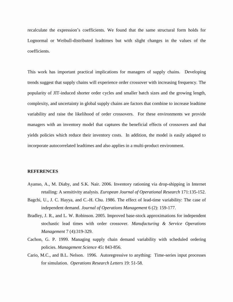
Thus (6) can be expressed as

0

0

2

0 | 0 0 0 0

0

( , ) ( , ) , ( )2 2

1( ( )) ( ) ( ) .

X X

X YsG sG

D D

R

X X W t

D k

R wNEC R k k G k G k

R R R

W k f W dW dt f dR

L

LL

L L

(A3)

Substituting 2 2 2XD

D

R v v

L L L and

2 2 2YD

D

v v

L L L into (A3) results in (7).

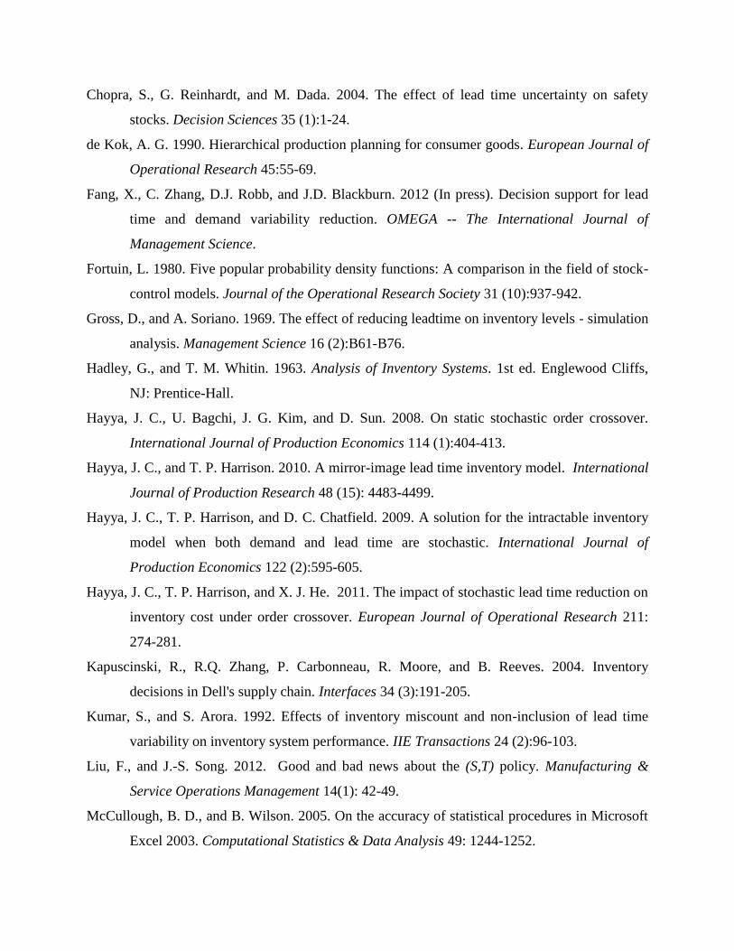
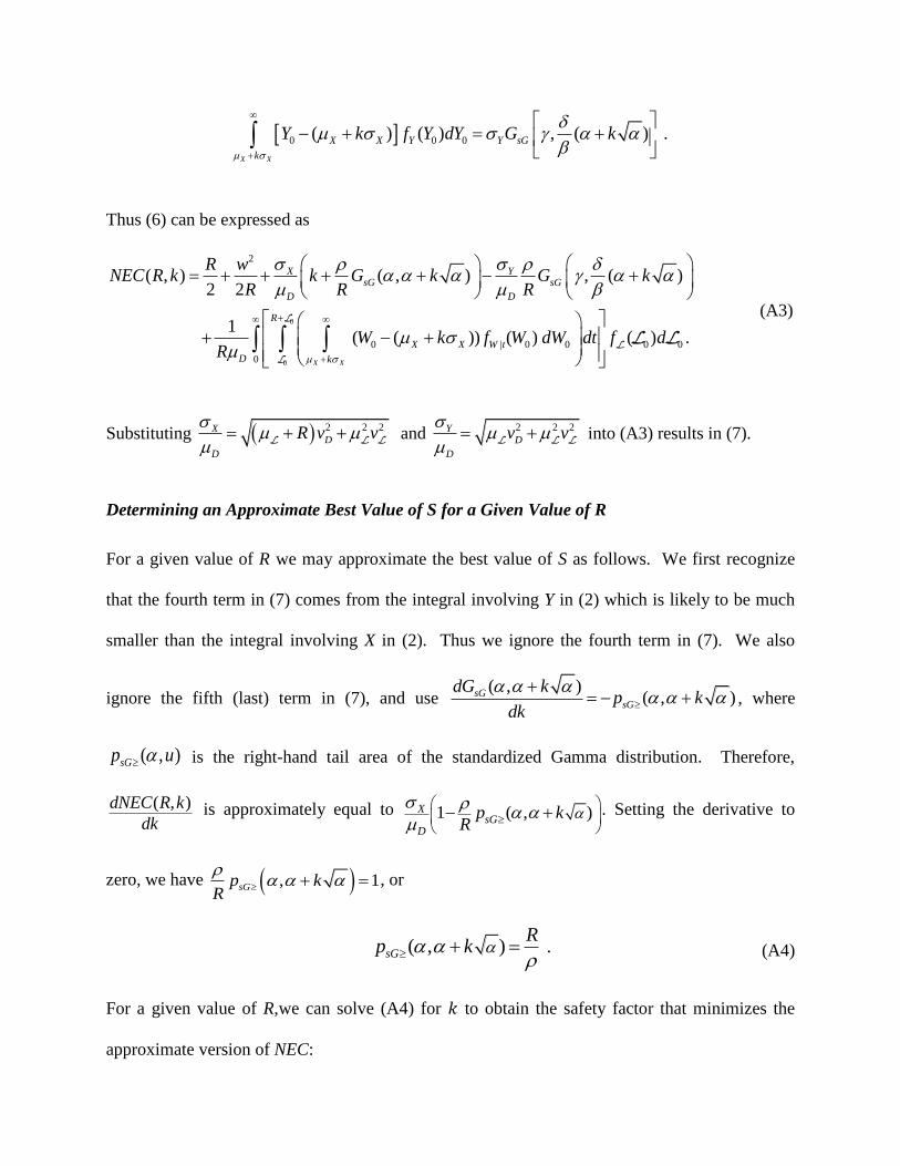
Determining an Approximate Best Value of S for a Given Value of R

For a given value of R we may approximate the best value of S as follows. We first recognize

that the fourth term in (7) comes from the integral involving Y in (2) which is likely to be much

smaller than the integral involving X in (2). Thus we ignore the fourth term in (7). We also

ignore the fifth (last) term in (7), and use ( , )

( , )sGsG

dG kp k

dk

, where

( , )sGp u is the right-hand tail area of the standardized Gamma distribution. Therefore,

( , )dNEC R k

dk is approximately equal to 1 ( , )X

sGD

p kR

. Setting the derivative to

zero, we have , 1sGp kR

, or

.( , )sG

Rp k

(A4)

For a given value of R,we can solve (A4) for to obtain the safety factor that minimizes the

approximate version of NEC:

11, ,ap

sG

Rk p

where 1 ,1sGp q

is the qth quantile of the standard Gamma distribution with parameter α.

Note that kap

may be obtained using a reverse lookup in Microsoft®

Excel, viz.,

1

1 , ,1 .R

GAMMAINV

In our own experimentation we utilized Mathematica, as problems have been observed with

inverse statistical functions in Excel (McCullough and Wilson, 2005).

Table 1: Some notation

A $ Fixed cost of each replenishment

B - Charge per unit short expressed as a multiple of c

c $/unit Unit variable cost of an item

D units/day Demand per day, distributed with mean and standard deviation ),( DD

EC $/day Expected total cost per unit time

k - Safety factor

L days Replenishment leadtime, with mean and standard deviation ),( LL

L days Effective leadtime, with mean and standard deviation ( , ) L L

NEC days Normalized expected total cost per unit time

r $/$/day Inventory holding charge

R days Reorder interval

S units Order-up-to level, XX kS

vD - Coefficient of variation of (daily) demand, vD = σD/μD

vL - Coefficient of variation of replenishment leadtime, vL = σL/μL

vL - Coefficient of variation of effective leadtime,

/v L L L

w days

The Economic Order Quantity expressed as a time interval, also known as

the Wilson number, cr

Aw

D

2

W | t units Demand during an interval of known length t

X units

Demand during the “protection interval” R L , distributed with mean and

standard deviation ),( XX . Coefficient of variation X

XXv

Y units Demand during the random effective leadtime L , distributed with mean and

standard deviation ,Y Y

α - The shape parameter of the X Gamma distribution

- The scale parameter of the X Gamma distribution

- The shape parameter of the Y Gamma distribution

- The scale parameter of the Y Gamma distribution

ρ days Shortage to holding cost ratio, ρ=B/r (i.e., the cost of holding one unit in

inventory for ρ days is equal to the cost of a shortage of one unit)

Table 2: Accuracy of the model in estimating the expected cost of (R, S) policies

Percentage difference,

analytic versus

simulated NEC

Absolute

percentage difference,

analytic versus

simulated NEC

w

1 0.7% 1.8%

20 0.1% 0.7%

100 0.0% 0.2%

ρ

100 0.0% 0.8%

500 0.3% 0.9%

2000 0.5% 1.0%

vD

0.0 1.0% 2.0%

2.5 0.1% 0.3%

5.0 -0.3% 0.4%

µL

4 0.2% 0.5%

25 -0.2% 0.9%

100 0.8% 1.3%

vL

0.00 -0.1% 0.2%

0.25 0.0% 1.0%

0.50 0.9% 1.5%

Average 0.3% 0.9%

Note: Results are averages across the 81 (=34) experiments in which the parameter in the first

column was set to the value shown in the second column. The last row gives the overall

averages across all 243 experiments.

Table 3: Performance of the analytic and heuristic approaches relative to the minimum cost

(R, S) policy

Percentage cost penalty due

to

using the

analytic solution

Additional percentage cost

penalty due to

using heuristic

w

1 1.0% 6.0%

20 0.2% 0.5%

100 0.3% 0.0%

ρ

100 0.2% 2.8%

500 0.4% 2.0%

2000 1.0% 1.7%

vD

0.0 1.1% 0.9%

2.5 0.1% 2.7%

5.0 0.3% 3.0%

µL

4 0.4% 1.2%

25 0.2% 1.8%

100 1.0% 3.5%

vL

0.00 0.1% 1.2%

0.25 0.5% 1.9%

0.50 0.9% 3.4%

Average 0.5% 2.2%

Note: Results are averages across the 81 (=34) experiments in which the parameter in the first

column was set to the value shown in the second column. The last row gives the overall

averages across all 243 experiments.

Table 4: Probability of crossover when L is used to determine R and S, and percentage cost

reduction due to using L

Probability of

crossover

using L

Percentage

reduction in cost

using L

w

1 30.5% 20.2%

20 10.4% 5.1%

100 1.3% 0.4%

Average 17.1% 2.2%

Note: These results are for 125 (out of 243) cases with nontrivial difference between L and L .

Results are averages across the cases in which w was set to the value shown in the second

column. The last row gives the overall averages across all 125 experiments.

Figure 1: The relationship between LR and

L L , based on simulated Gamma leadtimes

with various values of L and

L , including the fitted curve given in (1)

L

L

LR

0

0.2

0.4

0.6

0.8

1

0.02 0.2 2 20 200 2000

Gamma

Fitted Minimax