Analysis and Modeling of Analysis and Modeling of Climate ChangeClimate Change

A.K.M. Saiful IslamAssociate Professor, IWFM

Coordinator, Climate Change Study Cell

Bangladesh University of Engineer and Technology (BUET)

Training Course on Facing the Challenges of Climate Change: Issues, Impacts and adaptation Strategies for Bangladesh with focus on Water and Waste Management”

Organized by International Training Network (ITN) Centre, BUET

Presentation Outline

• Overview of the Climate System

• Modeling of Climate Change

• General Circulation Model (GCM)

• IPCC SRES Scenarios

• Regional Climate Model (RCM)

• Climatic Modeling at BUET

Climate Models

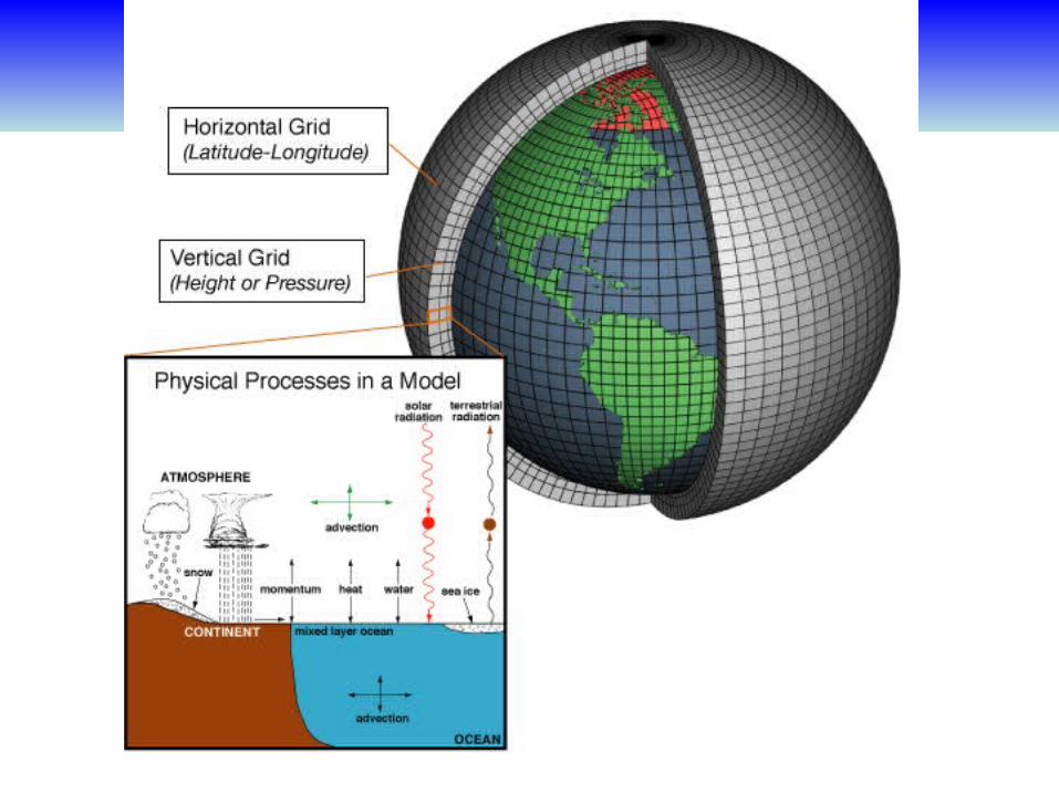
• Climate models are computer-based simulations that use mathematical formulas to re-create the chemical and physical processes that drive Earth’s climate. To “run” a model, scientists divide the planet into a 3-dimensional grid, apply the basic equations, and evaluate the results.

• Atmospheric models calculate winds, heat transfer, radiation, relative humidity, and surface hydrology within each grid and evaluate interactions with neighboring points. Climate models use quantitative methods to simulate the interactions of the atmosphere, oceans, land surface, and ice.

General Circulation Model (GCM)• General Circulation Models (GCMs) are a class of

computer-driven models for weather forecasting, understanding climate and projecting climate change, where they are commonly called Global Climate Models.

• Three dimensional GCM's discretise the equations for fluid motion and energy transfer and integrate these forward in time. They also contain parameterizations for processes - such as convection - that occur on scales too small to be resolved directly.

• Atmospheric GCMs (AGCMs) model the atmosphere and impose sea surface temperatures. Coupled atmosphere-ocean GCMs (AOGCMs, e.g. HadCM3, EdGCM, GFDL CM2.X, ARPEGE-Climate) combine the two models.

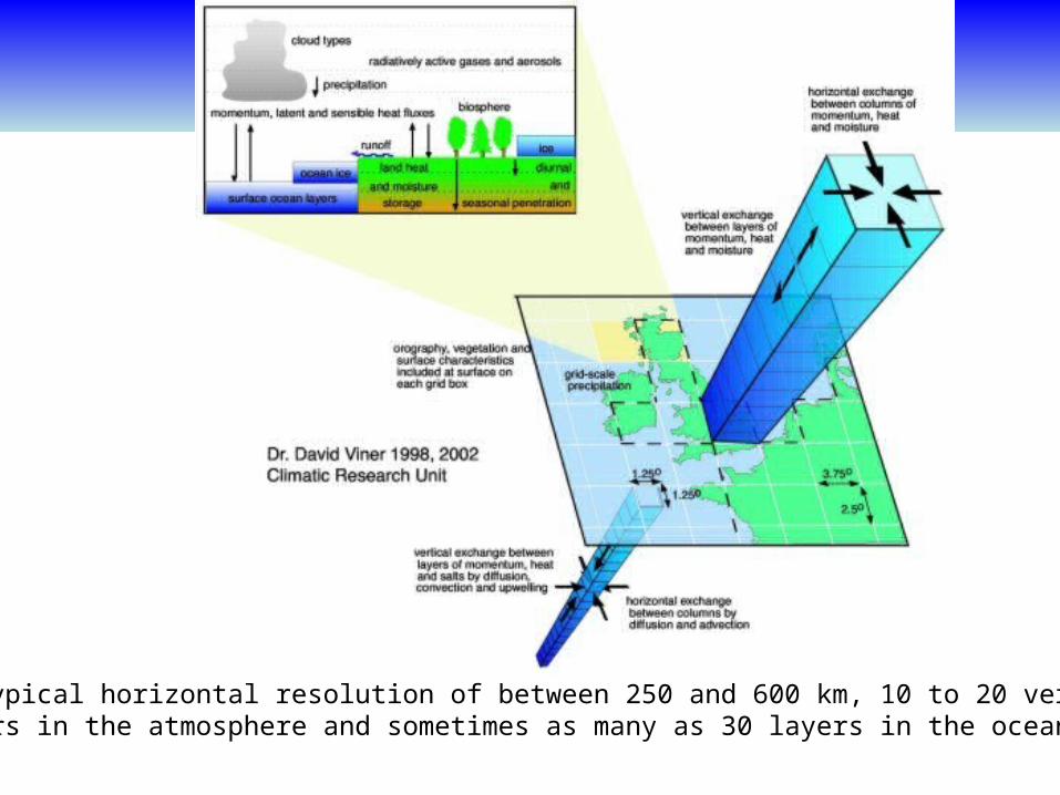
GCM typical horizontal resolution of between 250 and 600 km, 10 to 20 vertical layers in the atmosphere and sometimes as many as 30 layers in the oceans.

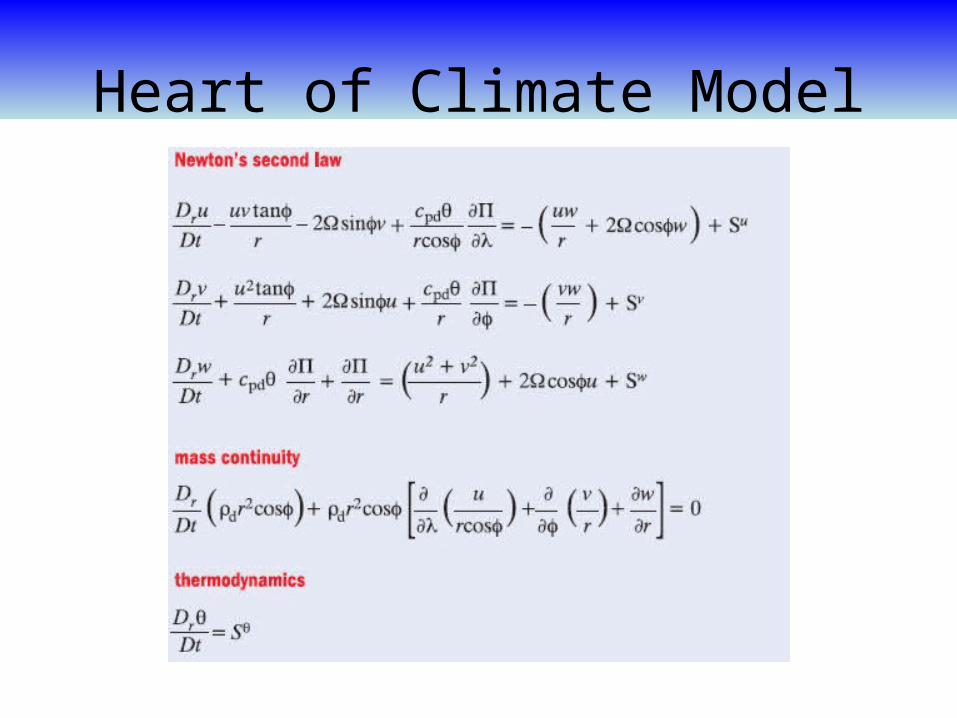
Heart of Climate Model

Complexity of GCM

Hardware Behind the Climate Model

• Geophysical Fluid Dynamics Laboratory

Special Report on Emissions Scenarios (SRES)

• The Special Report on Emissions Scenarios (SRES) was a report prepared by the Intergovernmental Panel on Climate Change (IPCC) for the Third Assessment Report (TAR) in 2001, on future emission scenarios to be used for driving global circulation models to develop climate change scenarios.

• It was used to replace the IS92 scenarios used for the IPCC Second Assessment Report of 1995. The SRES Scenarios were also used for the Fourth Assessment Report (AR4) in 2007.

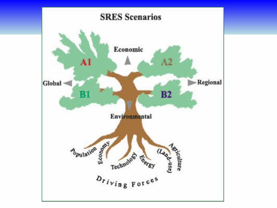
SERS Emission Scenarios• A1 - a future world of very rapid economic growth,

global population that peaks in mid-century and declines thereafter, and the rapid introduction of new and more efficient technologies. Three sub groups: fossil intensive (A1FI), non-fossil energy sources (A1T), or a balance across all sources (A1B).

• A2 - A very heterogeneous world. The underlying theme is that of strengthening regional cultural identities, with an emphasis on family values and local traditions, high population growth, and less concern for rapid economic development.

• B1 - a convergent world with the same global population, that peaks in mid-century and declines thereafter, as in the A1 storyline.

• B2 - a world in which the emphasis is on local solutions to economic, social and environmental sustainability.

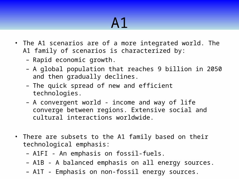
A1• The A1 scenarios are of a more integrated world. The A1

family of scenarios is characterized by:– Rapid economic growth.– A global population that reaches 9 billion in 2050 and

then gradually declines.– The quick spread of new and efficient technologies.– A convergent world - income and way of life converge

between regions. Extensive social and cultural interactions worldwide.

• There are subsets to the A1 family based on their technological emphasis:– A1FI - An emphasis on fossil-fuels.– A1B - A balanced emphasis on all energy sources.– A1T - Emphasis on non-fossil energy sources.

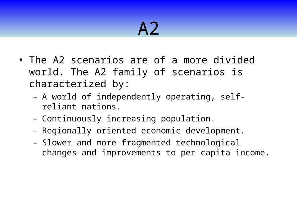
A2

• The A2 scenarios are of a more divided world. The A2 family of scenarios is characterized by:– A world of independently operating, self-reliant nations.– Continuously increasing population.– Regionally oriented economic development.– Slower and more fragmented technological changes and

improvements to per capita income.

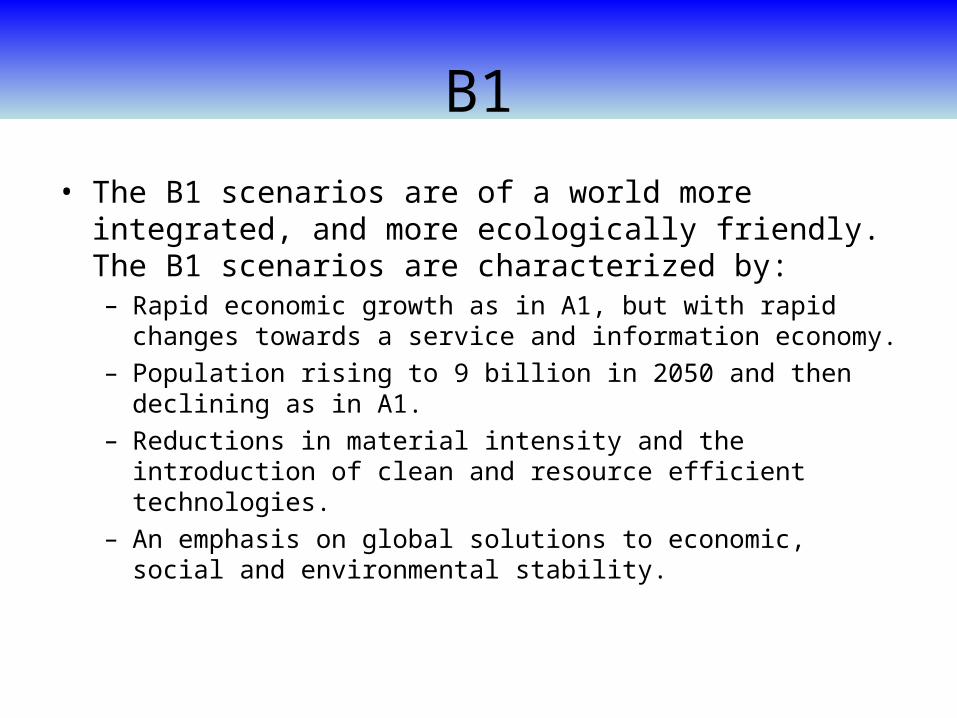
B1

• The B1 scenarios are of a world more integrated, and more ecologically friendly. The B1 scenarios are characterized by:– Rapid economic growth as in A1, but with rapid changes

towards a service and information economy.– Population rising to 9 billion in 2050 and then declining

as in A1.– Reductions in material intensity and the introduction of

clean and resource efficient technologies.– An emphasis on global solutions to economic, social and

environmental stability.

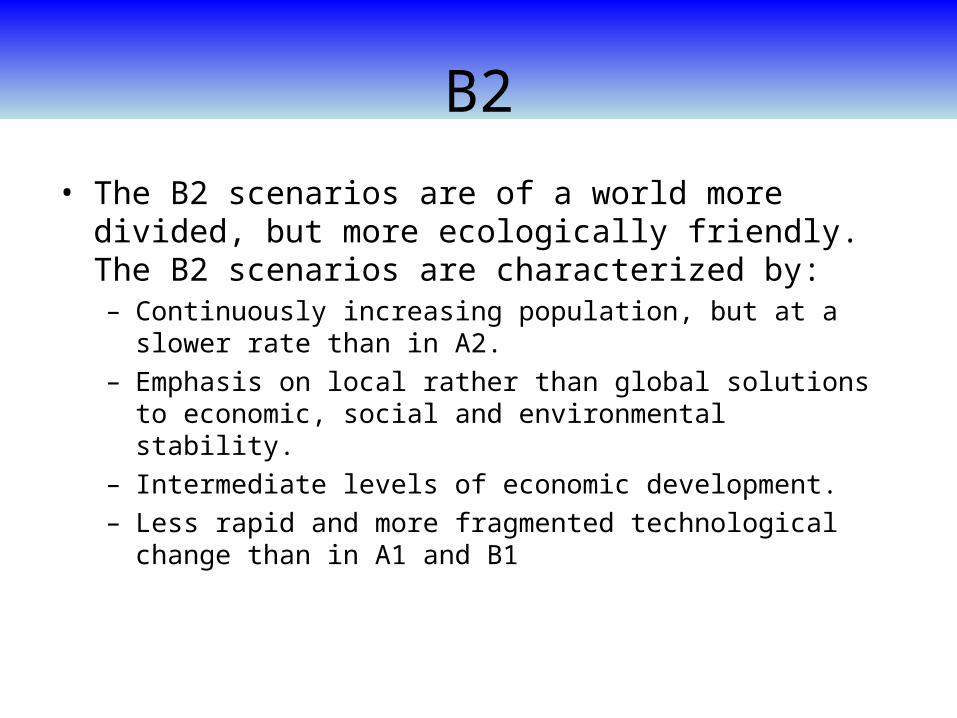
B2

• The B2 scenarios are of a world more divided, but more ecologically friendly. The B2 scenarios are characterized by:– Continuously increasing population, but at a slower rate

than in A2.– Emphasis on local rather than global solutions to

economic, social and environmental stability.– Intermediate levels of economic development.– Less rapid and more fragmented technological change

than in A1 and B1

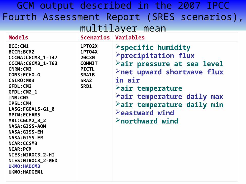
GCM output described in the 2007 IPCC Fourth Assessment Report (SRES scenarios), multilayer mean

Models Scenarios Variables

BCC:CM1BCCR:BCM2CCCMA:CGCM3_1-T47CCCMA:CGCM3_1-T63CNRM:CM3CONS:ECHO-GCSIRO:MK3GFDL:CM2GFDL:CM2_1INM:CM3IPSL:CM4LASG:FGOALS-G1_0MPIM:ECHAM5MRI:CGCM2_3_2NASA:GISS-AOMNASA:GISS-EHNASA:GISS-ERNCAR:CCSM3NCAR:PCMNIES:MIROC3_2-HINIES:MIROC3_2-MEDUKMO:HADCM3UKMO:HADGEM1

1PTO2X1PTO4X20C3MCOMMITPICTLSRA1BSRA2SRB1

specific humidityprecipitation fluxair pressure at sea levelnet upward shortwave flux in airair temperatureair temperature daily maxair temperature daily mineastward windnorthward wind

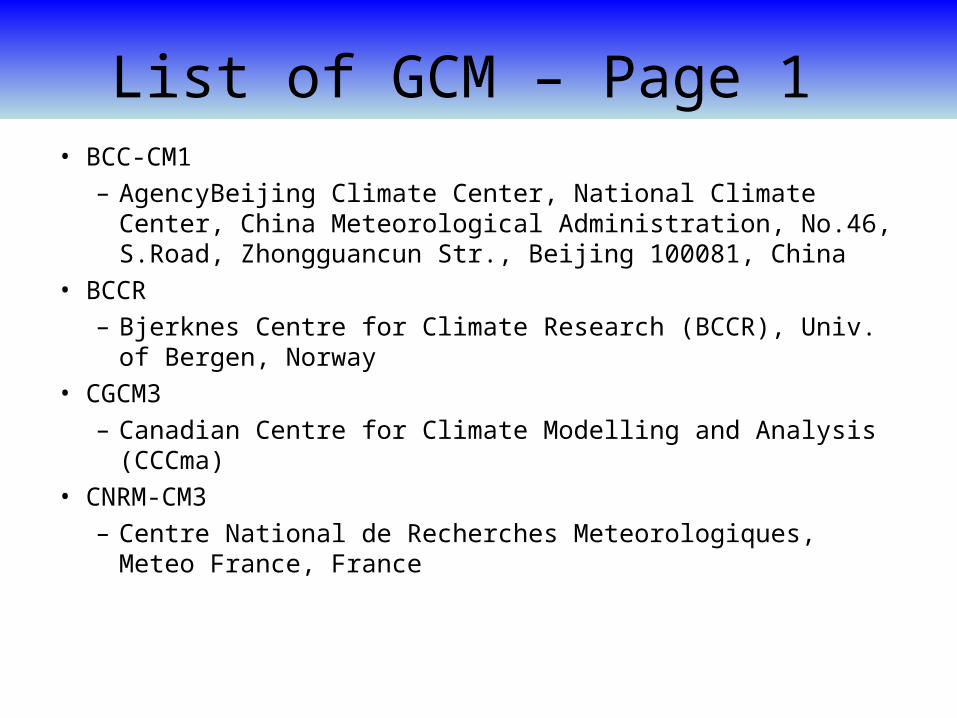
List of GCM – Page 1 • BCC-CM1

– AgencyBeijing Climate Center, National Climate Center, China Meteorological Administration, No.46, S.Road, Zhongguancun Str., Beijing 100081, China

• BCCR – Bjerknes Centre for Climate Research (BCCR), Univ. of

Bergen, Norway • CGCM3

– Canadian Centre for Climate Modelling and Analysis (CCCma)

• CNRM-CM3 – Centre National de Recherches Meteorologiques, Meteo

France, France

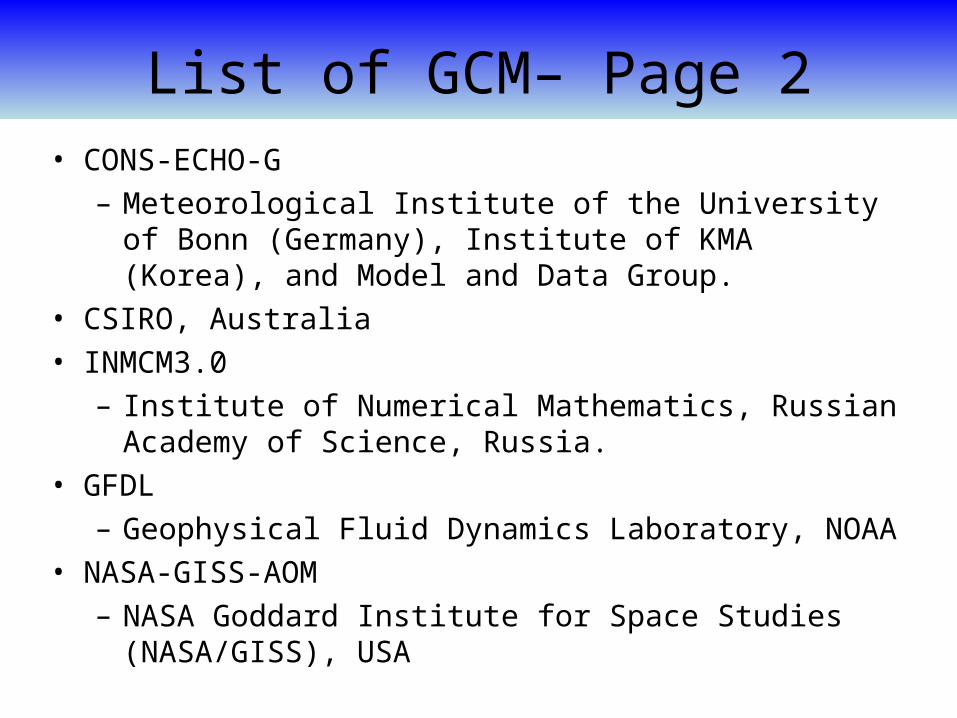
List of GCM– Page 2• CONS-ECHO-G

– Meteorological Institute of the University of Bonn (Germany), Institute of KMA (Korea), and Model and Data Group.

• CSIRO, Australia • INMCM3.0

– Institute of Numerical Mathematics, Russian Academy of Science, Russia.

• GFDL– Geophysical Fluid Dynamics Laboratory, NOAA

• NASA-GISS-AOM – NASA Goddard Institute for Space Studies

(NASA/GISS), USA

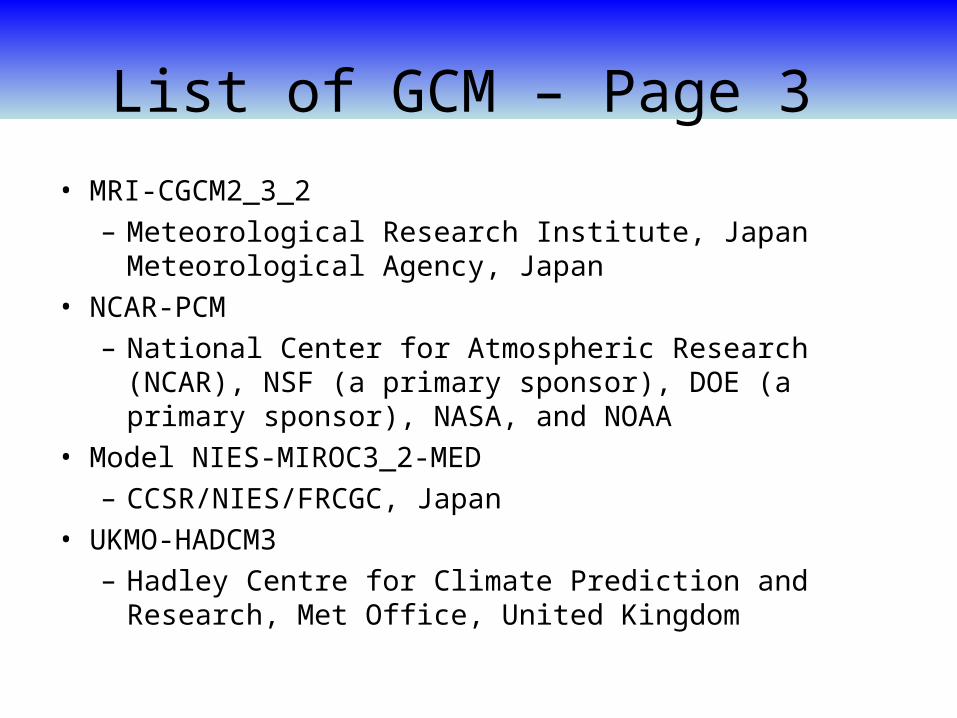
List of GCM – Page 3

• MRI-CGCM2_3_2 – Meteorological Research Institute, Japan

Meteorological Agency, Japan • NCAR-PCM

– National Center for Atmospheric Research (NCAR), NSF (a primary sponsor), DOE (a primary sponsor), NASA, and NOAA

• Model NIES-MIROC3_2-MED – CCSR/NIES/FRCGC, Japan

• UKMO-HADCM3 – Hadley Centre for Climate Prediction and Research,

Met Office, United Kingdom

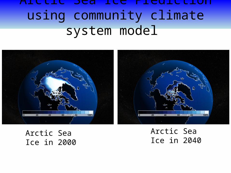
Arctic Sea Ice Prediction using community climate system model

Arctic Sea Ice in 2040

Arctic Sea Ice in 2000

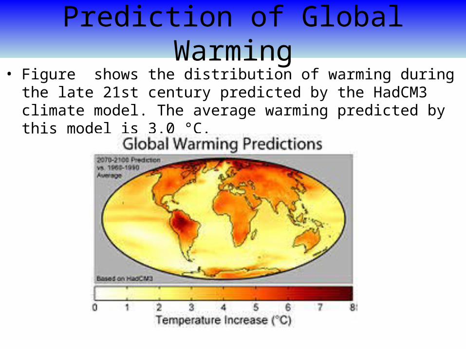
Prediction of Global Warming• Figure shows the distribution of warming during the

late 21st century predicted by the HadCM3 climate model. The average warming predicted by this model is 3.0 °C.

Prediction of Temperature increase

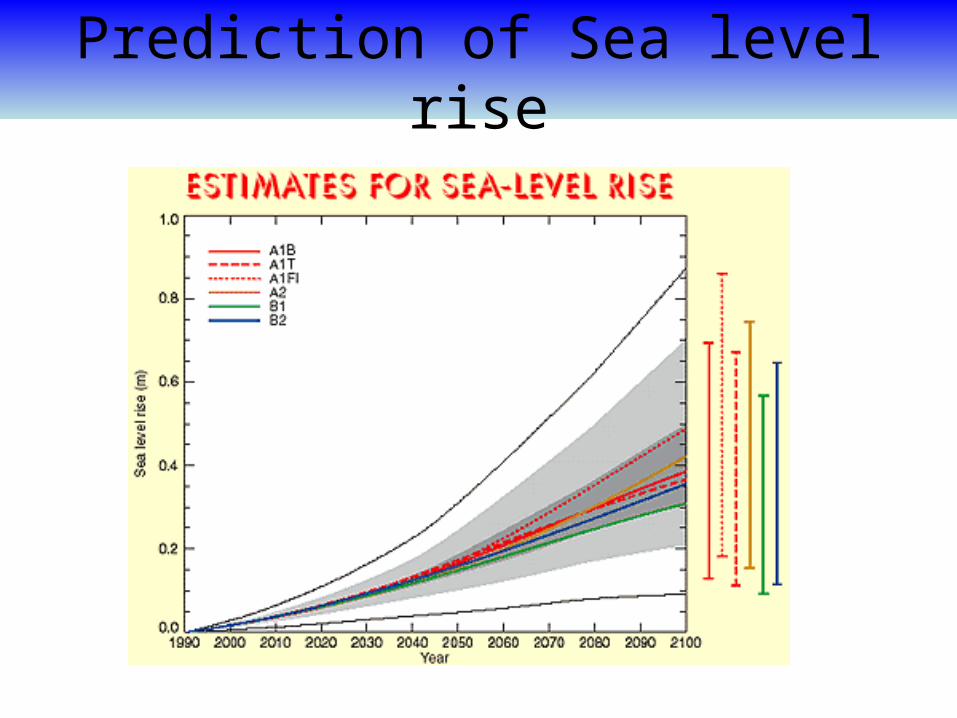
Prediction of Sea level rise

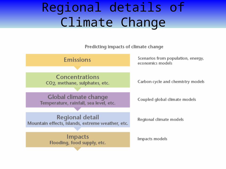
Regional details of Climate Change

Regional Climate modeling

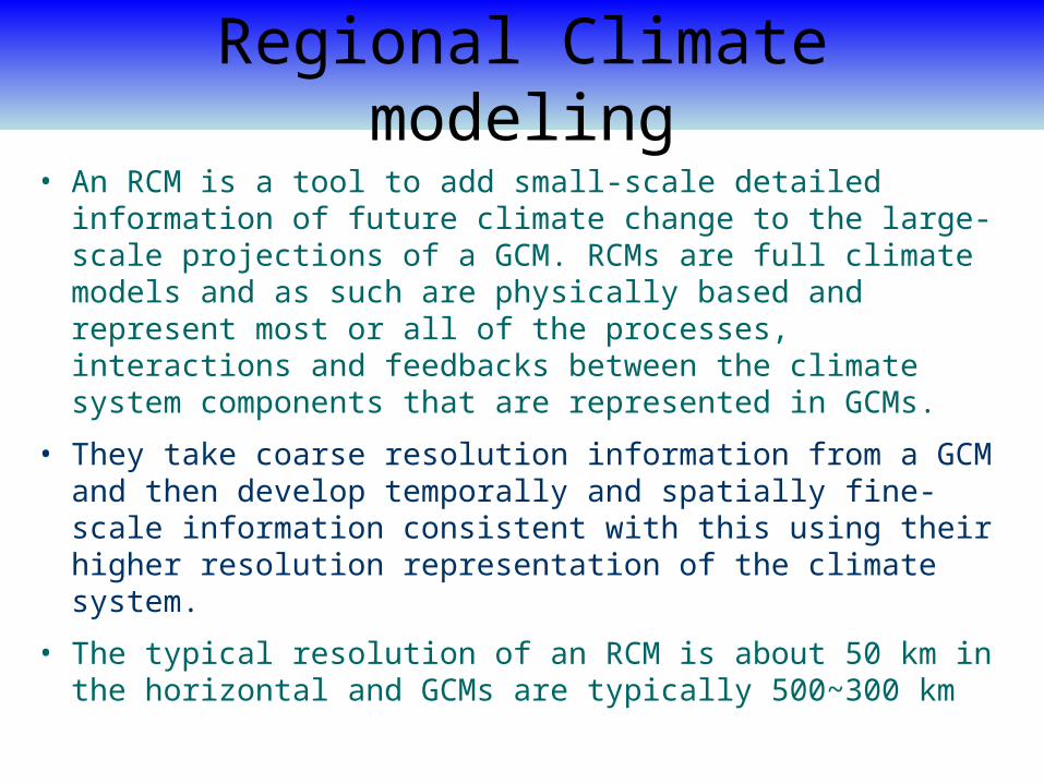
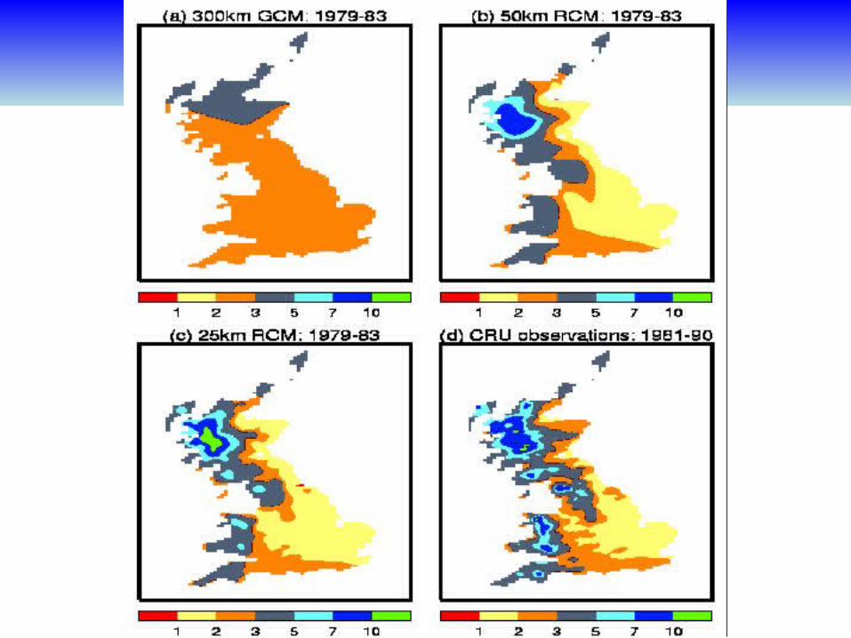
• An RCM is a tool to add small-scale detailed information of future climate change to the large-scale projections of a GCM. RCMs are full climate models and as such are physically based and represent most or all of the processes, interactions and feedbacks between the climate system components that are represented in GCMs.

• They take coarse resolution information from a GCM and then develop temporally and spatially fine-scale information consistent with this using their higher resolution representation of the climate system.

• The typical resolution of an RCM is about 50 km in the horizontal and GCMs are typically 500~300 km

RCM can simulate cyclones and hurricanes

Regional Climate change modeling in Bangladesh

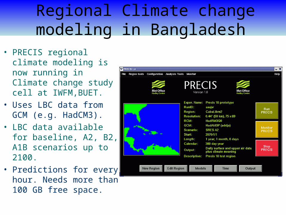
• PRECIS regional climate modeling is now running in Climate change study cell at IWFM,BUET.

• Uses LBC data from GCM (e.g. HadCM3).

• LBC data available for baseline, A2, B2, A1B scenarios up to 2100.

• Predictions for every hour. Needs more than 100 GB free space.

Domain used in PRECIS experiment

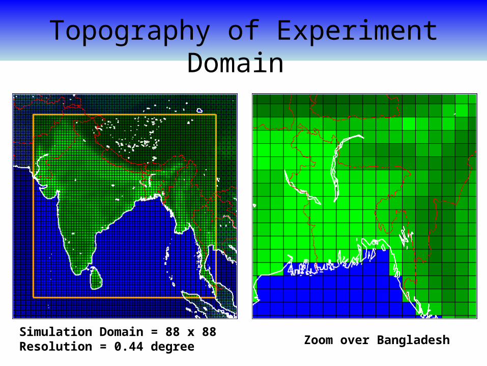
Topography of Experiment Domain

Zoom over BangladeshSimulation Domain = 88 x 88 Resolution = 0.44 degree

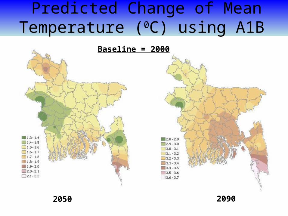
Predicted Change of Mean Temperature (0C) using A1B

2050 2090

Baseline = 2000

Predicting Maximum Temperature using A2 Scenarios

[Output of PRECIS model using SRES A2 scenario]

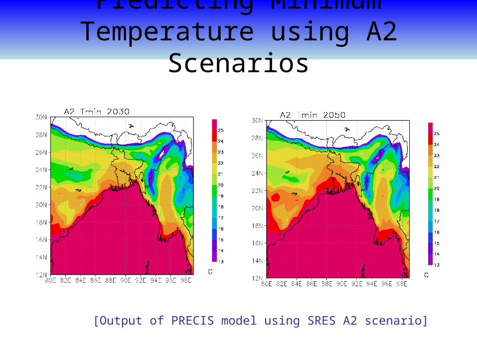
[Output of PRECIS model using SRES A2 scenario]

Predicting Minimum Temperature using A2 Scenarios

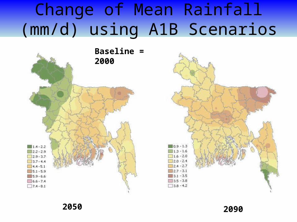
Change of Mean Rainfall (mm/d) using A1B Scenarios

2050 2090

Baseline = 2000

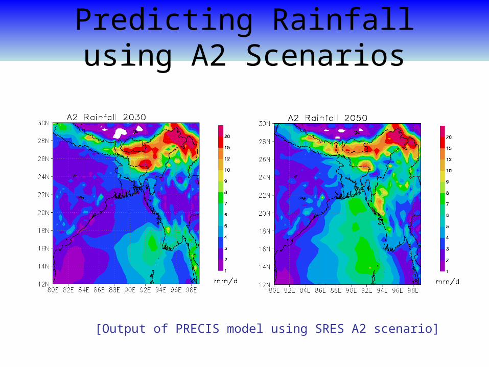
Predicting Rainfall using A2 Scenarios

[Output of PRECIS model using SRES A2 scenario]

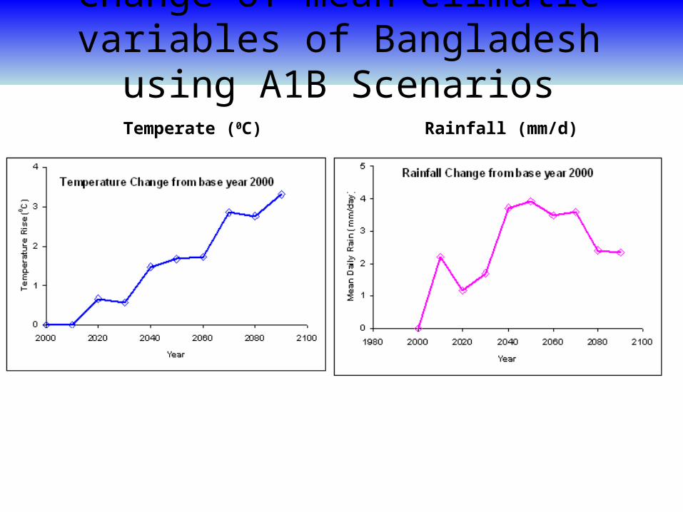
Change of mean climatic variables of Bangladesh using A1B Scenarios

Temperate (0C) Rainfall (mm/d)

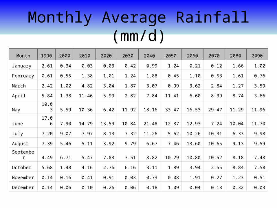
Monthly Average Rainfall (mm/d)

Month 1990 2000 2010 2020 2030 2040 2050 2060 2070 2080 2090

January 2.61 0.34 0.03 0.03 0.42 0.99 1.24 0.21 0.12 1.66 1.02

February 0.61 0.55 1.38 1.01 1.24 1.88 0.45 1.10 0.53 1.61 0.76

March 2.42 1.02 4.82 3.04 1.87 3.07 0.99 3.62 2.84 1.27 3.59

April 5.84 1.38 11.46 5.99 2.82 7.84 11.41 6.60 8.39 8.74 3.66

May10.0

3 5.59 10.36 6.42 11.92 18.16 33.47 16.53 29.47 11.29 11.96

June17.0

6 7.90 14.79 13.59 10.84 21.48 12.87 12.93 7.24 10.04 11.70

July 7.20 9.07 7.97 8.13 7.32 11.26 5.62 10.26 10.31 6.33 9.98

August 7.39 5.46 5.11 3.92 9.79 6.67 7.46 13.60 10.65 9.13 9.59

September 4.49 6.71 5.47 7.83 7.51 8.82 10.29 10.80 10.52 8.18 7.48

October 5.68 1.48 4.16 2.76 6.16 3.11 1.89 3.94 2.55 8.84 7.58

November 0.14 0.16 0.41 0.91 0.03 0.73 0.08 1.91 0.27 1.23 0.51

December 0.14 0.06 0.10 0.26 0.06 0.18 1.09 0.04 0.13 0.32 0.03

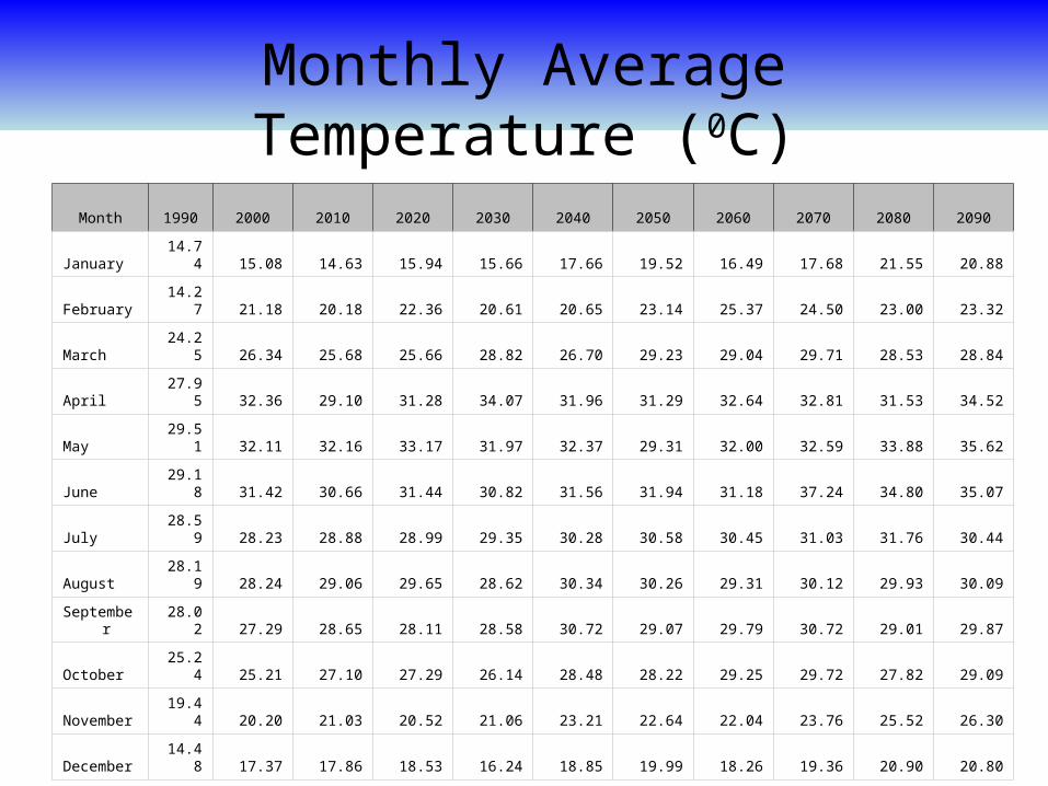
Monthly Average Temperature (0C)

Month 1990 2000 2010 2020 2030 2040 2050 2060 2070 2080 2090

January 14.74 15.08 14.63 15.94 15.66 17.66 19.52 16.49 17.68 21.55 20.88

February 14.27 21.18 20.18 22.36 20.61 20.65 23.14 25.37 24.50 23.00 23.32

March 24.25 26.34 25.68 25.66 28.82 26.70 29.23 29.04 29.71 28.53 28.84

April 27.95 32.36 29.10 31.28 34.07 31.96 31.29 32.64 32.81 31.53 34.52

May 29.51 32.11 32.16 33.17 31.97 32.37 29.31 32.00 32.59 33.88 35.62

June 29.18 31.42 30.66 31.44 30.82 31.56 31.94 31.18 37.24 34.80 35.07

July 28.59 28.23 28.88 28.99 29.35 30.28 30.58 30.45 31.03 31.76 30.44

August 28.19 28.24 29.06 29.65 28.62 30.34 30.26 29.31 30.12 29.93 30.09

September 28.02 27.29 28.65 28.11 28.58 30.72 29.07 29.79 30.72 29.01 29.87

October 25.24 25.21 27.10 27.29 26.14 28.48 28.22 29.25 29.72 27.82 29.09

November 19.44 20.20 21.03 20.52 21.06 23.21 22.64 22.04 23.76 25.52 26.30

December 14.48 17.37 17.86 18.53 16.24 18.85 19.99 18.26 19.36 20.90 20.80

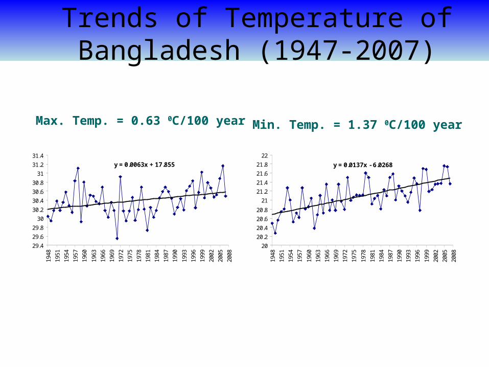
Trends of Temperature of Bangladesh (1947-2007)

y = 0.0063x + 17.855

29.4

29.6

29.8

30

30.2

30.4

30.6

30.8

31

31.2

31.4

1948

1951

1954

1957

1960

1963

1966

1969

1972

1975

1978

1981

1984

1987

1990

1993

1996

1999

2002

2005

2008

Trends of Maximum Temperature

y = 0.0137x - 6.0268

20

20.2

20.4

20.6

20.8

21

21.2

21.4

21.6

21.8

22

1948

1951

1954

1957

1960

1963

1966

1969

1972

1975

1978

1981

1984

1987

1990

1993

1996

1999

2002

2005

2008

Trends of Minimum Temperature

Max. Temp. = 0.63 0C/100 year Min. Temp. = 1.37 0C/100 year

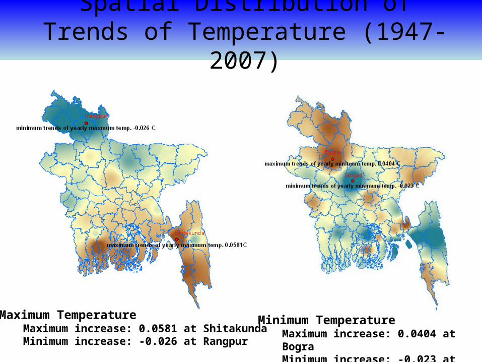
Maximum TemperatureMaximum increase: 0.0581 at ShitakundaMinimum increase: -0.026 at Rangpur

Minimum TemperatureMaximum increase: 0.0404 at BograMinimum increase: -0.023 at Tangail

Spatial Distribution of Trends of Temperature (1947-2007)

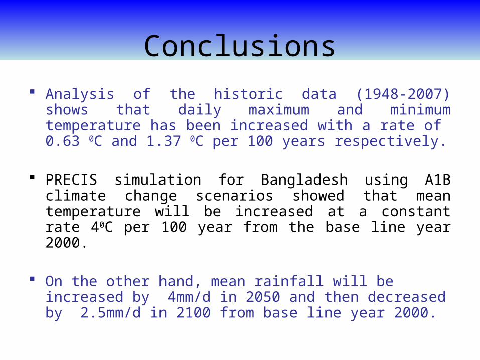
Conclusions

Analysis of the historic data (1948-2007) shows that daily maximum and minimum temperature has been increased with a rate of 0.63 0C and 1.37 0C per 100 years respectively.

PRECIS simulation for Bangladesh using A1B climate change scenarios showed that mean temperature will be increased at a constant rate 40C per 100 year from the base line year 2000.

On the other hand, mean rainfall will be increased by 4mm/d in 2050 and then decreased by 2.5mm/d in 2100 from base line year 2000.

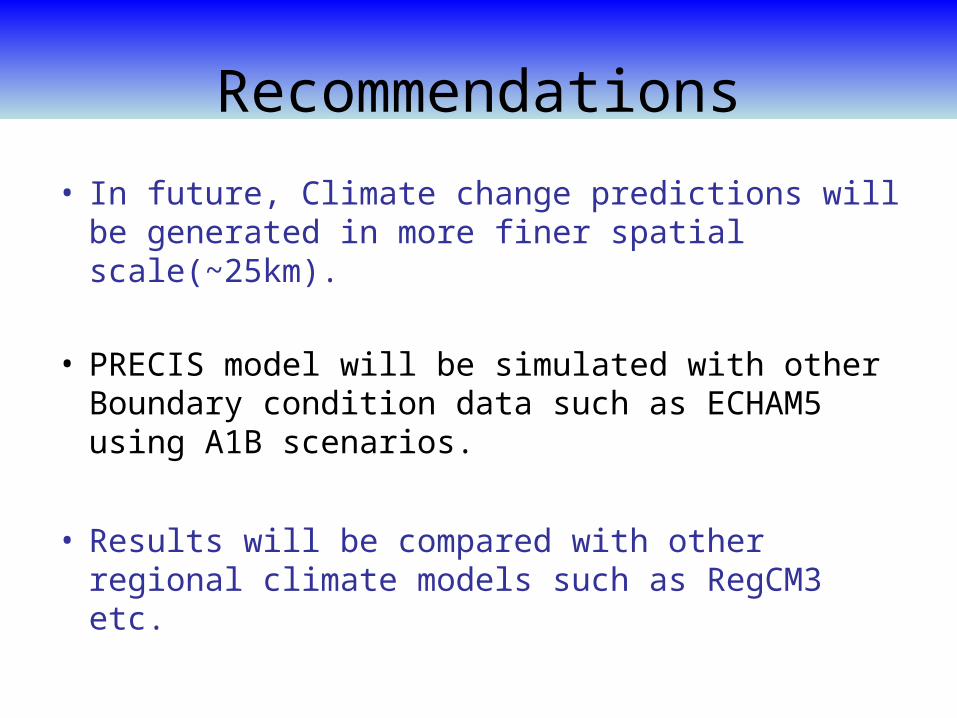
Recommendations

• In future, Climate change predictions will be generated in more finer spatial scale(~25km).

• PRECIS model will be simulated with other Boundary condition data such as ECHAM5 using A1B scenarios.

• Results will be compared with other regional climate models such as RegCM3 etc.

Climate Change Study Cell, BUET http://teacher.buet.ac.bd/diriwfm/climate/

Thank you