Embed Size (px)
Citation preview
ANALYSIS AND MODELING OF PLASTIC WRINKLING
IN DEEP DRAWING
A THESIS SUBMITTED TO THE GRADUATE SCHOOL OF NATURAL AND APPLIED SCIENCES
OF MIDDLE EAST TECHNICAL UNIVERSITY
BY
SERHAT YALÇIN
IN PARTIAL FULLFILLMENT OF THE REQUIREMENTS FOR
THE DEGREE OF MASTER OF SCIENCE IN
MECHANICAL ENGINEERING
SEPTEMBER 2010

Approval of the thesis:
ANALYSIS AND MODELING OF PLASTIC WRINKLING IN DEEP DRAWING
submitted by SERHAT YALÇIN in partial fulfillment of the requirements for the degree of Master of Science in Mechanical Engineering Department, Middle East Technical University by, Prof. Dr. Canan Özgen Dean, Graduate School of Natural and Applied Sciences ________________ Prof. Dr. Süha Oral Head of the Department, Mechanical Engineering ________________ Prof. Dr. Süha Oral Supervisor, Mechanical Engineering, METU ________________ Prof. Dr. Bilgin Kaftanoğlu Co-supervisor, Mechanical Engineering, METU ________________ Examining Committee Members: Prof. Dr. Haluk Darendeliler Mechanical Engineering, METU _________________ Prof. Dr. Suha Oral Mechanical Engineering, METU _________________ Prof. Dr. Bilgin Kaftanoğlu Mechanical Engineering, METU _________________ Assoc. Prof. Dr. Serkan Dağ Mechanical Engineering, METU _________________ Prof. Dr. Ali Kalkanlı Metallurgical and Materials Engineering, METU _________________
Date: 16.09.2010

iii
I hereby declare that all information in this document has been obtained and presented in accordance with academic rules and ethical conduct. I also declare that, as required by these rules and conduct, I have fully cited and referenced all material and results that are not original to this work.
Name, Last name: Serhat YALÇIN
Signature:

iv
ABSTRACT
ANALYSIS AND MODELLING OF PLASTIC WRINKLING IN DEEP
DRAWING
Yalçın, Serhat
M.Sc., Department of Mechanical Engineering
Supervisor: Prof. Dr. Suha Oral
Co-Supervisor: Prof. Dr. Bilgin Kaftanoğlu
September 2010, 116 pages
Deep drawing operations are crucial for metal forming operations and
manufacturing. Obtaining a defect free final product with the desired mechanical
properties is very important for fulfilling the customer expectations and market
competitions. Wrinkling is one of the fatal and most frequent defects that must be
prevented. This study focuses on understanding the phenomenon of wrinkling and
probable precautions that can be applied. In this study, dynamic – explicit
commercial finite element code is used to simulate deep drawing process. The
numerical experiments are compared with NUMISHEET benchmarks in order to
verify the reliability of the finite element code and analysis parameters.
In order to understand plastic wrinkling, the effect of blank holder force is
investigated. Axisymmetrical numerical models of a cup are investigated with
different blank holder forces. Wrinkling instability is illustrated in energy diagrams
of the process. Effect of anisotropy on wrinkling is also discussed by comparing

v
isotropic and anisotropic numerical experiments with the material as steel. Different
drawbead models, both equivalent and physical, are implied to the problem and
results are discussed.
Besides numerical analysis, experimental verification is also conducted as
conventional deep drawing operation by a hydraulic press. This yields to the ability
to understand the effect of blank thickness on wrinkling formation through numerical
and experimental analyses. The wave formations of different sized blanks with four
different thicknesses are illustrated.
Keywords: Wrinkling, Deep Drawing, Finite Element Method, Sheet Metal
Forming, Blank Holder Force, Drawbead, Anisotropy

vi
ÖZ
DERİN ÇEKME İŞLEMLERİNDE PLASTİK BURUŞMA ANALİZİ VE
MODELLEMESİ
Yalçın, Serhat
Yüksek Lisans, Makina Mühendisliği Bölümü
Tez Yöneticisi: Prof. Dr. Suha Oral
Ortak Tez Yöneticisi: Prof. Dr. Bilgin Kaftanoğlu
Eylül 2010, 116 sayfa
Derin çekme işlemleri metal şekillendirme ve üretimde çok önemlidir. Müşteri
Memnuniyeti ve Pazar rekabetini karşılamak amacıyla istenilen mekanik özelliklerde
olan kusursuz son ürün elde çok önemlidir. Tehlikeli ve sık görülen kusurlardan biri
olan buruşma engellenmelidir. Bu çalışma buruşma fenomenini ve uygulanabilir
önlemleri anlamaya odaklanmıştır. Bu çalışmada derin çekme işlemlerini simule
edebilmek için dinamik-açık ticari sonlu elemanlar kodu kullanılmıştır. Sayısal
deneyler NUMISHEET referansları ile kıyaslanarak sonlu elemanlar kodunun
hassasiyeti doğrulanmıştır.
Plastik buruşmayı anlamak için baskı plakası kuvvetinin buruşmaya olan etkisi
araştırılmıştır. Değişik baskı plakası kuvvetleri için eksenel simetrik kap

vii
modellemesi incelenmiştir. Buruşma kararsızlığı işlemin enerji grafiklerinde
gösterilmiştir. Buruşmadaki anizotropi etkisi çelik malzemelerde, izotropik ve
izotropik olmayan nümerik deneyler karşılaştırılarak tartışılmıştır. Pot çemberi
modellemesi, eş ve fiziksel olarak, probleme eklenmiş ve sonuçları tartışılmıştır.
Sayısal analizlere ilaveten, hidrolik pres kullanılarak klasik derin çekme
işleminin deneysel doğrulama çalışması yapılmıştır. Bu çalışma sayesinde, sayısal ve
deneysel analizler ile parça kalınlığının buruşmaya etkisi anlaşılmıştır. Farklı
ölçülerdeki parçalarda, dalga oluşumu 4 ayrı kalınlık değeri için gösterilmiştir.
Anahtar Kelimeler: Buruşma, Derin Çekme, Sonlu Elemanlar Analizi, Saç Metal
Şekillendirme, Baskı Plakası Kuvveti, Pot Çemberi, Anizotropi

viii
To My Family & Darling

ix
ACKNOWLEDGEMENTS
I would like to express my gratefulness and appreciation to my supervisor Prof. Dr.
Suha Oral and my co-supervisor Prof. Dr. Bilgin Kaftanoğlu for their guidance,
encouragement, advice and insight throughout the study.
I wish to thank again Prof. Dr. Bilgin Kaftanoğlu for providing me the facilities for
my study. I also would like to thank to all employees of the Metal Forming Centre of
Excellence in Atılım University and the Metal Forming Lab in METU for their help
in performing experiments.
I also want to express my gratitude to Mr. Ahmet Kurt from ASELSAN for his
comments and suggestions throughout the study.
I thank to Mr. İ. Erkan Önder for supplying experimental data of NUMISHEET
benchmark and his support in the early stages of my work.
I thank to Mr. Servet Gündüz from Yıldırım Alüminyum for his support to my work.
Thanks to my friends Berkay Şanay, Celalettin Yumuş and Cankat Saçlı for their
support and friendship. I also wish to thank my colleagues Türker Gürer, Bengi
Demirçivi and Yavuz Selim Kayserilioğlu from ASELSAN.
I specially thank to Duygu Şen whose friendship, support, motivation and never
ending patience made great contributions to this work.
Finally, I also want to thank my beloved family, my mother Serap Yalçın, my father
Nihat Yalçın, my brother Serkan Yalçın for their encouragement and faith in me.

x
TABLE OF CONTENTS
ABSTRACT................................................................................................................ iv
ÖZ ............................................................................................................................... vi
ACKNOWLEDGEMENTS ........................................................................................ ix
TABLE OF CONTENTS............................................................................................. x
LIST OF FIGURES ...................................................................................................xii
LIST OF TABLES .................................................................................................... xvi
CHAPTERS
1. INTRODUCTION ................................................................................................... 1
2. SURVEY OF LITERATURE.................................................................................. 6
2.1 Introduction ............................................................................................................ 6
2.2 Deep Drawing Process ........................................................................................... 6
2.2.1 Stress Zones during Deep Drawing............................................................. 8
2.3 Other Deep Drawing Technologies...................................................................... 11
2.4 Anisotropy............................................................................................................ 14
2.5 The Limiting Drawing Ratio................................................................................ 15
2.6 Formability of Sheet Metals................................................................................. 18
2.6.1 Forming Limit Diagrams........................................................................... 21
2.7 Previous Studies ................................................................................................... 23
3. OBJECT OF THE PRESENT STUDY.................................................................. 28
4. THEORY OF FINITE ELEMENT METHOD...................................................... 30
4.1 Introduction .......................................................................................................... 30
4.2 History of Finite Element Method ....................................................................... 30
4.3 Basics of Finite Element Method......................................................................... 31
4.3.1 Finite Element Procedures ........................................................................ 33
4.3.2 Element Stiffness Matrix........................................................................... 34
4.3.3 Shape Function.......................................................................................... 35

xi
4.3.4 Transformation Matrix .............................................................................. 36
4.4 Algorithms of Numerical Simulation Solvers...................................................... 38
4.4.1 Differences between Implicit and Explicit Approaches............................ 38
4.4.2 Dynamic- Explicit Finite Element Method............................................... 40
4.4.3 Plastic Work.............................................................................................. 46
4.5 Features of PAM-STAMP 2G.............................................................................. 47
5. NUMERICAL AND EXPERIMENTAL RESULTS ............................................ 50
5.1 Introduction .......................................................................................................... 50
5.2 Benchmark Problem............................................................................................. 51
5.2.1 Process Parameters.................................................................................... 53
5.2.2 Punch Velocity .......................................................................................... 54
5.2.3 Element Size and Refinement ................................................................... 59
5.2.4 Mesh Topology ......................................................................................... 64
5.2.5 Comparison with NUMISHEET 2002 Benchmarks ................................. 67
5.3 Wrinkling Simulations ......................................................................................... 70
5.3.1 Blank Holder Simulations ......................................................................... 70
5.3.2 Drawbead Simulations .............................................................................. 79
5.4 Experimental Study.............................................................................................. 94
5.4.1 Tension Test .............................................................................................. 94
5.4.2 Conventional Deep Drawing Experiment ................................................. 96
6. DISCUSSION ...................................................................................................... 102
7. CONCLUSION.................................................................................................... 107
REFERENCES......................................................................................................... 107
APPENDICES
A. NUMISHEET 2002 BENCHMARK PARTICIPANTS..................................... 107
B. TINIUS OLSEN TESTING MACHINE............................................................. 112

xii
LIST OF FIGURES
FIGURES
Figure 1.1 Automobile parts produced by deep drawing............................................. 2
Figure 1.2 Conventional Deep Drawing Process ......................................................... 2
Figure 1.3 Basic Tools in Deep Drawing..................................................................... 3
Figure 1.4 Deep Drawn Parts ....................................................................................... 3
Figure 1.5 Various failure modes in Deep Drawing: 1-Flange wrinkling; 2-Wall
wrinkling; 3-Part wrinkling; 4-Ring prints; 5-Traces; 6-Orange skin; 7-Lüder’s strips;
8-Bottom fracture; 9-Corner fracture; 10,11,12-Folding; 13,14-Corner folding ......... 4
Figure 2.1 Geometry parameters for deep drawing tools............................................. 7
Figure 2.2 Four different zones in deep drawing ......................................................... 9
Figure 2.3 Pressing forces in deep drawing of a round cup with a blank holder ......... 9
Figure 2.4 Principle of High Pressure Sheet Forming: ..................................................
a) Beginning of process, b) end of free bulging, c) end of cavity filling................... 13
Figure 2.5 Principle of hydromechanical deep drawing ............................................ 14
Figure 2.6 Effect of average strain ratio on LDR for different materials .................. 17
Figure 2.7 Effect of relative punch diameter on the limiting drawing ratio .............. 17
Figure 2.8 Bursting, wrinkling and tearing observed in analysis............................... 18
Figure 2.9 Formability of sheet metals ...................................................................... 19
Figure 2.10 Working window in deep drawing ......................................................... 20
Figure 2.11 Methods used for evaluating the sheet metal formability....................... 21
Figure 2.12 Grid of small circles are printed or etched on sheet metal ..................... 22
Figure 2.13 FLD Experiment ..................................................................................... 23
Figure 4.1 Finite Element Mesh structure.................................................................. 31
Figure 4.2 Input parameters of Finite Element Method............................................. 33
Figure 4.3 Elasto-Plastic and Rigid-Plastic material behaviors ................................. 34
Figure 4.4 General Element ....................................................................................... 34

xiii
Figure 4.5 Simple two node element ......................................................................... 35
Figure 4.6 Local and Global Coordinate system of an element................................. 36
Figure 4.7 Simple one dimensional mass-spring-damper system.............................. 40
Figure 4.8 PAM-STAMP 2G Modules ...................................................................... 48
Figure 5.1 Tool geometry of Benchmark problem .................................................... 51
Figure 5.2 True Stress vs. True Strain curve of DDQ mild steel ............................... 52
Figure 5.3 Mesh structures of Half and Full model ................................................... 54
Figure 5.4 Punch speed effect on thickness distribution of a 5mm Element Size ..... 55
Figure 5.5 Punch speed effect on thickness distribution of a 3mm Element Size ..... 56
Figure 5.6 Punch Force vs. Punch Progression curves for different Punch Velocities
.................................................................................................................................... 57
Figure 5.7 Punch Force vs. Punch Progression curves for unacceptable Punch
Velocities.................................................................................................................... 57
Figure 5.8 Punch Speed effect on Computational Time for 5mm mesh size............. 58
Figure 5.9 Fillet mesh detail of the Die ..................................................................... 59
Figure 5.10 Refinement procedures ........................................................................... 60
Figure 5.11 Angle Criteria ......................................................................................... 61
Figure 5.12 Geometrical Criterion ............................................................................. 61
Figure 5.13 Thickness variations of 3mm, 5mm, 5mm/2Ref, 5mm/3Ref for Punch
Speed 500mm/s. ......................................................................................................... 62
Figure 5.14 Punch Force vs. Punch Progression curves for different element sizes . 63
Figure 5.15 Punch Speed and Element size effect on Computational Time.............. 63
Figure 5.16 Uniform and Radial Mesh of the blank .................................................. 64
Figure 5.17 Equivalent plastic strain contours of radial and uniform mesh structures
.................................................................................................................................... 65
Figure 5.18 Punch Force vs. Punch Progression curves for Radial and Uniform mesh
structures .................................................................................................................... 66
Figure 5.19 Wrinkled blank with uniform and radial mesh structures ...................... 66
Figure 5.20 Comparison of Punch Force – Punch Stroke curve of steel HBHF
simulation with Benchmark Experiments .................................................................. 68
Figure 5.21 Comparison of outer circumference of steel flanges of simulation........ 69

xiv
Figure 5.22 Comparison of outer circumference of steel flanges of simulation........ 69
Figure 5.23 Deep drawn blank without Blank holder ................................................ 71
Figure 5.24 Deep drawn parts with different blank holder forces and corresponding
wave formations ......................................................................................................... 71
Figure 5.25 Wave Formations for 1 mm, 5 mm, 10 mm, 15 mm and 20 mm Punch
Depths with simulations of 1 N , 1000 N and 3000N Blank Holder Forces.............. 73
Figure 5.26 Further analysis images for finding required blankholder force. ........... 75
Figure 5.27 Energy Graphs for 5000 N Blank Holder Force..................................... 76
Figure 5.28 External Energy Graphs versus Punch Progression for 1000 N, 5000 N
and 10000 N Blank Holder Forces............................................................................. 77
Figure 5.29 Anisotropic and Isotropic Material wave formations ............................. 78
Figure 5.30 Drawbead models of Pam Stamp............................................................ 80
Figure 5.31 Restraining and Opening Force of the Equivalent Drawbead model ..... 81
Figure 5.32 Drawbead model in reality and in simulation......................................... 81
Figure 5.33 Thickness distributions for different groove depths at 20 mm punch
depth........................................................................................................................... 82
Figure 5.34 Drawbead models for 70 mm, 80 mm and 90 mm ................................. 83
Figure 5.35 Thickness contours for 70 mm, 80 mm and 90 mm radii drawbeads..... 83
Figure 5.36 Fully drawn part with 90 mm drawbead................................................. 84
Figure 5.37 Wrinkled blank due to insufficient blank holder force........................... 85
Figure 5.39 Drawbead added simulation models....................................................... 86
Figure 5.40 Small drawbead analyses for 10 kN BHF............................................... 87
Figure 5.41 Large drawbead analyses for 10 kN BHF............................................... 88
Figure 5.42 Small drawbead analyses for 100 kN BHF............................................. 89
Figure 5.43 Large drawbead analyses for 100 kN BHF............................................. 90
Figure 5.44 Inclined drawbead dimensions ............................................................... 91
Figure 5.45 Thickness contours for inclined drawbead model with 100 kN BHF .... 92
Figure 5.46 Mesh structure before and after the simulation ...................................... 93
Figure 5.47 External energy diagrams for different drawbead models...................... 94
Figure 5.48 Universal Tensile Testing Machine with 30 ton force capacity (Zwick)95
Figure 5.49 Tension Test specimens, 2 mm thickness, before and after the test ....... 96

xv
Figure 5.50 Tinius Olsen Tesing Machine................................................................. 97
Figure 5.51 Deep Drawn parts with different thickness and different diameters ...... 98
Figure 5.52 Wrinkling formations for 80 mm blanks ................................................ 98
Figure 5.53 Wrinkling formations for 100 mm blanks .............................................. 99
Figure 5.54 Finite Element Model of the experiment tools ..................................... 100
Figure 5.55 Experimented and Simulated deep drawn part ..................................... 100
Figure 5.56 Wrinkling formations for 80 mm diameter blanks ............................... 100
Figure 5.57 Wrinkling formations for 90 mm diameter blanks ............................... 101
Figure 5.58 Wrinkling formations for 100 mm diameter blanks ............................. 101

xvi
LIST OF TABLES
TABLES
Table 4.1 Main Differences in Explicit and Implicit Approaches ............................. 39
Table 5.1 Material properties of DDQ mild steel ...................................................... 52
Table 5.2 Number and Amplitude of Waves for increasing Blank Holder Forces for
20 mm Draw Depth.................................................................................................... 72
Table 5.3 Number and Amplitude of Waves for increasing Blank Holder Forces for
40 mm Draw Depth.................................................................................................... 74
Table 5.4 Number and Amplitude of Waves for finding the required Blank Holder
Force for 40 mm Draw Depth .................................................................................... 74
Table 5.5 Number of Waves for Anisotropic and Isotropic Materials....................... 79
Table 5.6 Drawbead geometry parameters................................................................. 81
Table 5.7 Drawbead Dimensions in milimeters......................................................... 86
Table 5.8 Material Properties of AL 1050 Material for four thickness values .......... 96
Table 5.9 Experiment and Simulation results for specified blank diameters for
different thicknesses................................................................................................. 101
Table A.1 Participant information of AE-01............................................................ 113
Table A.2 Participant information of AE-02............................................................ 113
Table A.3 Participant information of AE-03............................................................ 113
Table A.4 Participant information of AE-04............................................................ 114
Table A.5 Participant information of AE-05............................................................ 114
Table A.6 Participant information of AE-06............................................................ 114
Table A.7 Participant information of AE-07............................................................ 115
Table B.1 Specifications of Tinius Olsen A-40 Testing Machine ........................... 116

1
CHAPTER 1
INTRODUCTION
Casting, machining, welding and metal forming are the main methods of
manufacturing [1]. The other methods of manufacturing are powder metallurgy, heat
treatment and finishing. In casting a liquid material is poured into a mold and then
allowed to solidify in order to take the desired shape. By casting, big and complex
parts can be manufactured. The second manufacturing process is machining. This
process can be defined as removing material (chips) from the workpiece. Machining
is one of the most used processes in manufacturing. Cutting tool is used for removing
material from the piece while cooling fluid dissipates the heat generated from the
process. Another method is welding. In this method, two or more metal pieces are
joined together by melting or fusing them with the help of heat. Welding is generally
used in ship building, automotive manufacturing and aerospace applications. The last
method is metal forming. In this process the material shape is formed by applying
force to the piece. Metal forming is used for achieving complex shape products and
improving the strength of the material. During forming, little material is wasted
compare to other manufacturing processes. Bulk forming and sheet metal working
are the two main groups of forming processes based on raw material used in the
process. Rolling, forging and extrusion in bulk forming can be done cold, warm and
hot. The other forming process is sheet metal forming. In this method, thin sheets of
metal are shaped by applying pressure through dies. Sheet metal forming is very
important for metals because nearly %50 of metals is produced in sheet metals. [2]
Sheet metal forming is done by many ways such as shearing and blanking,
bending stretching, spinning and deep drawing. Those methods are widely used for
producing various products in different places of industry. The parts manufactured
by sheet metal forming are widely used in automotive and aircraft industries.

2
Figure 1.1 Automobile parts produced by deep drawing
Deep drawing is one of the most important sheet metal forming processes. A 2-d
part is shaped into a 3-d part by deep drawing. According to the definition in DIN
8584, “deep drawing is the tensile-compressive forming of a sheet blank to a hollow
body open on one side or the forming of a pre-drawn hollow shape into another with
a smaller cross-section without an intentional change in the sheet thickness.”
Figure 1.2 Conventional Deep Drawing Process [3]
3
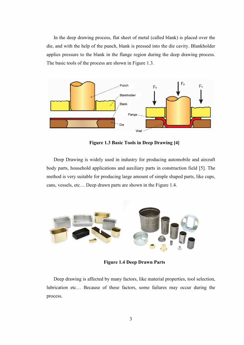
In the deep drawing process, flat sheet of metal (called blank) is placed over the
die, and with the help of the punch, blank is pressed into the die cavity. Blankholder
applies pressure to the blank in the flange region during the deep drawing process.
The basic tools of the process are shown in Figure 1.3.
Figure 1.3 Basic Tools in Deep Drawing [4]
Deep Drawing is widely used in industry for producing automobile and aircraft
body parts, household applications and auxiliary parts in construction field [5]. The
method is very suitable for producing large amount of simple shaped parts, like cups,
cans, vessels, etc… Deep drawn parts are shown in the Figure 1.4.
Figure 1.4 Deep Drawn Parts
Deep drawing is affected by many factors, like material properties, tool selection,
lubrication etc… Because of these factors, some failures may occur during the
process.

4
Tearing, necking, wrinkling, earing and poor surface appearance are the main
failure types that can be seen in deep drawing, see the Figure 1.5. Tearing and
necking are tensile instability caused by strain localization. The strength of the part is
reduced and the appearance worsened because of tearing and necking. Another
failure is wrinkling, caused by compressive stresses unlike to tearing and necking.
Plastic buckling occurs because of the high compressive stress and waves formed on
the part. The other one is earing. On the walls of the totally drawn part earing can be
seen. The main reason for earing is planar plastic anisotropy. Also the last defect
types which poorly affect the appearance of the sheet metal part are ring prints,
traces, orange skin (or orange peel structure), and Lüders strips.
Figure 1.5 Various failure modes in Deep Drawing: 1-Flange wrinkling; 2-Wall wrinkling; 3-Part wrinkling; 4-Ring prints; 5-Traces; 6-Orange skin; 7-Lüder’s strips; 8-Bottom fracture; 9-Corner fracture; 10,11,12-Folding; 13,14-Corner
folding. [2]
A part wrinkled during the deep drawing process, will not be accepted and most
likely become a scrap, a total waste of both money and time. Because of these
reasons, wrinkling must be prevented. There are two main methods used in order to
prevent wrinkling. The former is using a blankholder. Blankholder is a tool used for
preventing the edge of a sheet metal part from wrinkling. There are two main
blankholder types available namely, clearance and pressure type blankholder. In the
former, the sheet metal kept at a constant thickness by adjusting fixed distance
between blankholder and die, during the process and wrinkling is prevented. In the
latter, force is applied to the blank from the blankholder, called blank holder force
(BHF), in order to prevent wrinkling. Adjusting the BHF is very important, because

5
high BHF leads to fracture at the cup wall and low BHF leads to wrinkling in the
flange of the cup.
The other method is using drawbead in the flange region. Drawbeads are placed
to the die (small protrusions on the die surface) in order to control the flow of the
material during the forming operations. The material fills the groove, this results in a
change in the strain distribution in the flange region. Thinning of the blank is
achieved and compressive stresses are decreased so wrinkling is avoided.
In manufacturing processes the main goal is to obtain defect free end product.
The first step of manufacturing is the designing process, which enormously affects
the whole manufacturing process. The designer must have knowledge about possible
problems and their solutions during production. Many researches have been
completed in various manufacturing processes because of the knowledge needed to
achieve better quality product. This thesis will discuss about flange wrinkling
problem and its prevention in the deep drawing process.
The whole thesis composed of seven chapters. The first chapter is about the
general information about the study. In the next chapter, the literature survey about
deep drawing process, wrinkling problem and previous work on deep drawing will be
discussed. Third chapter defines the object of the study. The fourth chapter is
dedicated to the Finite Element Method and PAM-STAMP, commercial Finite
Element program. In the next chapter, numerical and experimental data obtained
throughout the study will be given. The discussion of these results will be discussed
in chapter six. Finally, conclusions of this study will be presented in the last chapter.

6
CHAPTER 2
SURVEY OF LITERATURE
2.1 Introduction
This chapter presents the literature search related to the current study. First,
conventional deep drawing process will be discussed. Secondly, sheet metal
formability concept is mentioned and possible failure modes are discussed. Then,
wrinkling and its prevention are stated. At the end of the chapter, previous researches
related to the mentioned concepts are presented.
2.2 Deep Drawing Process
As mentioned in the introduction chapter, flat sheet of metal is formed into a 3-d
product by deep drawing process. The main tools of the process are blank, punch, die
and blankholder. In the simple circular cup drawing process with blankholder, the
tools and tool geometries are shown in the Figure 2.1.

7
Figure 2.1 Geometry parameters for deep drawing tools
The tool geometry parameters are stated as;
• Punch Radius Rp
• Punch Edge Radius rp
• Blank Thickness t
• Blank Radius Rb
• Die Radius Rd
• Die Edge Radius rd
These parameters must be selected very carefully because the final product
highly depends on these geometries. Shape of the fully drawn cup is obtained by
selecting die and punch respectively. Clearance is also an important parameter,
formulated as the difference between die radius and punch radius (c = Rd – Rp). If
the clearance is not large enough, ironning will occur. Ironning is defined as thinning

8
of the blank at the die cavity. In order to eliminate this problem, clearance should be
%25 larger than the initial blank thickness. Also the punch edge radius and die edge
radius effects the process. Larger corner radius lowers the punch load whereas
smaller radius increases the needed punch load.
In addition to the tool geometry parameters, there are also physical parameters in
drawing operations. Some of these are classified as;
• Blank material properties
• Blank holder force
• Punch speed
• Lubrication
• Draw depth
2.2.1 Stress Zones during Deep Drawing
Deep drawing process is defined as a tensile-compressive forming of the sheet
metal in the literature. During the deep drawing process, due to punch force and
blankholder force, different stress zones are formed. Four different states can be
defined as Force application zone, Force transmission zone, Bending zone and
Forming zone, that can be seen from the Figure 2.2.

9
Figure 2.2 Four different zones in deep drawing [6]
The punch force is applied onto the bottom of the drawn part, which is called the
force application zone. Then it is transferred to the flange region. The force is
transmitted along the wall of the cup. Bending happens over the die edge radius and
forming takes places in the flange region.
Figure 2.3 Pressing forces in deep drawing of a round cup with a blank holder
[4]

10
The workpiece is subjected to radial tension forces FR and tangential compression
forces FT during the process (Figure 2.3). The material is compressed in the
tangential direction and stretched in the radial direction. As it can be seen from the
figure above, there are compressive forces in the flange region and tensile forces
elsewhere in the workpiece. [4]
Over the punch head, force application zone, sliding and stretching of the
material occurs. In this region, material gets thinner because of stretching. The
limiting drawing ratio (LDR), will be discussed later, depends on the load carrying
capacity of this zone. The maximum load carrying capacity is determined by the
plastic instability taking place in this region. However, plastic instability depends on
the friction properties between the punch and blank. Equ-biaxial tensile stresses act
in this region.
In the region between die and punch, force transmission zone, generally there is
no contact of the material with either of punch and die. This is a transition region
between die and punch. In this region radial tensile stresses act on the material.
Material gets thinner and tearing or necking can take place in this region.
Over the die edge radius, sliding and bending of the material occurs. In this
region, in the radial direction tensile stresses occurs, whereas compressive stress is
observed in the circumferential direction. As mentioned before, radius of the
curvature of die profile has effect on the punch load. For a sharper radius, more
plastic bending work is done, therefore the punch load increases. In the bending
region, material gets thinner due to bending under tensile stresses in the radial
direction.
In the flange region pure radial drawing occurs. There is a circumferential
compressive stress and a radial tensile stress state in this region. This is the only
region that the material gets thicker because of the compressive stress. There is a
possibility of bulging in the flange region due to compressive forces. When the
compressive forces at the flange region exceed a certain limit, wrinkling occurs.

11
Therefore, the blank holding forces, and sometimes the drawbeads, are utilized to
control the flowing of the material into the die cavity to overcome compressive
forces’ effects.
As the draw depth is increased, the amount of deformation and the deformation
resistance are also increased. The sheet metal is most severely stretched in the corner
of the draw punch, corresponding to the tip of the drawn cup. Failure normally
occurs at this region of the blank.
Since there is a strongly non-homogeneous deformation throughout the part,
residual stresses arise. Residual tension is observed on the outside whereas residual
compression occurs in the inside of the part over the die lip in axial direction. These
residual stresses are caused by bending and unbending action happened over the die.
Through the wall of the drawn part, residual stresses takes its largest value near the
top of the wall, near the intersection area of wall and die lip, due to bending. The
wall of the part is subjected to bending moment because of residual stresses. This
moment is leveled by the hoop tension, occurring at the top of the cup. Hoop tension
can cause stress corrosion cracking at the transmission zone (wall) in some metal
materials.
Owing to the presence of residual stresses, deep drawn parts are sensitive to
successive operations. A workpiece may distort or fracture upon machining
operations and heat treatments may cause the part to change shape.
2.3 Other Deep Drawing Technologies
There are alternative deep drawing methods which make use of active media and
active energy. Active media include formless solid substances such as sand or steel
balls, fluids (oil, water) and gases, whereby the forming work is performed by a press
using a method similar to that employed with the rigid tools. Hydroforming is the
general name for this soft-tool forming technology. Rubber pad forming and fluid

12
tool forming are types of soft tool forming technologies. For instance, in Geurin and
Marform processes the die is replaced with a rubber path and the punch is solid.
In hydroforming, die or punch is replaced by oil, water or other fluid media. In
order words the rigid tool force is replaced by the fluid pressure. The main groups of
hydroforming are Tube hydroforming and Sheet hydroforming. Tube hydroforming
is a cold forming process. During the process, a tube is subjected to pressure from the
inside and at the same time it is compressed in axial or radial direction. Just like deep
drawing processes, during tube drawing process some instability phenomena may
occur. Bursting, buckling and wrinkling can be observed throughout the tube
hydroforming. [2]
Sheet hydroforming is divided into two types; called high-pressure sheet forming
and hydromechanical deep drawing. In high pressure sheet forming, pressurized fluid
is used for the replacement of the punch. The process is composed of two stages,
called free bulging and cavity filling stage, shown in the Figure 2.4. Lower
springback and lower residual stress values are the main advantages of the process.

13
Figure 2.4 Principle of High Pressure Sheet Forming:
a) Beginning of process, b) end of free bulging, c) end of cavity filling
However, in hydromechanical deep drawing, die is replaced by a pressurized
fluid. The main stages of the process are shown in the Figure 2.5. The main
advantages of the process are obtaining higher drawing ratio, better surface quality
and lower springback of the product.

14
Figure 2.5 Principle of hydromechanical deep drawing
Hydroforming is a commonly used technique in the industry. Over recent years,
the process gained popularity on three main groups: The automotive industry (cross
members, side members, manifolds, roof rails, spoilers, gear shafts, seat frame
components...), domestic appliance industry (tube bends, T-fittings...) and pipe
component manufacturers (intake pipes...).
2.4 Anisotropy
Due to their crystallographic structure and the characteristic of the rolling
process, sheet metals generally exhibit a significant anisotropy of mechanical
properties. The variation of their plastic behavior with direction is assessed by a
quantity called Lankford parameter of anisotropy coefficient. This coefficient is
usually obtained by uniaxial tensile tests on strip shaped sheet specimens. The
anisotropy coefficient (r) is defined by
2
3
rεε
= (2.1)
Where ε2 is the strain in the width direction and ε3 is in the thickness direction.
Experiments show that “r” depends on the in-plane direction. If the tensile
specimen is cut having its longitudinal axis parallel to the rolling direction, the
coefficient r90 is obtained. The average of the r-values obtained for different

15
directions in the plane of the sheet metal represents the coefficient of normal
anisotropy rn. The coefficient of normal anisotropy is obtained from equation
0 45 902
4n
r r rr
+ ⋅ += (2.2)
where
r0 is anisotropy factor in rolling direction
r45 is anisotropy factor in 45° direction relative to rolling direction
r90 is anisotropy factor in 90° direction relative to rolling direction
A material with a high rn value will experience less thinning during a deep
drawing operation than a material having a smaller rn value, provided that their flow
characteristics are identical. For instance, aluminum usually has an r value smaller
than 1 (about 0.6), whereas steel has an rn value larger than 1 (about 1.5).
A measure of the variation of normal anisotropy with the angle to the rolling
direction is known as planar anisotropy. The equation for planar anisotropy is given
as;
0 45 902
4
r r rr
− ⋅ +∆ = (2.3)
This value can be negative or positive. For instance, steels usually have positive
∆r. As stated before, planar anisotropy is directly related to earing. As the magnitude
of the ∆r value increases, the ear heights increase. Therefore for deep drawing
operations, suitable materials must have smaller planar anisotropy values in
magnitude.
2.5 The Limiting Drawing Ratio
The limiting draw ratio is the ratio of the diameter of the initial blank form to the
diameter of the drawn part. LDR is an important numerical value for cylindrical draw
parts in determining the required number of drawing steps. For cylindrical cup

16
drawing process with circular cross-section, drawing ratio can be defined by the
following equation:
0.MAX
p
dLDR
d= (2.4)
Here, d0. MAX is the maximum blank diameter that can be fully drawn to a cup
without any failure and dP is the punch diameter.
The drawing ratio is dependent on many factors like the tool geometry,
lubrication conditions, and the amount of blank holding forces, sheet thickness, and
material properties (especially the r and n value). The limiting drawing ratio (LDR),
which can be reached in a single drawing step, is theoretically calculated by
membrane analysis. The ideal limiting drawing ratio found from the membrane
theory is
2.72MAXLDR e≤ ≈ (2.5)
In reality the LDR for aluminum sheets are 1.8 to 2.0. This value is around 1.9 to
2.2 for steel sheets. The reason for this is various process parameters are not
considered in the simplifying membrane theory.
For any material in a deep drawing operation, a higher LDR means that ‘deeper’
drawings are possible, whereas a lower LDR restricts the deep drawability. The LDR
is strongly material dependent and for several materials the effect of average strain
ratio on LDR can be seen from the Figure 2.6

17
Figure 2.6 Effect of average strain ratio on LDR for different materials [7]
Also the blank thickness and the punch diameter affect the LDR. Limiting
drawing ratio decreases as the relative punch diameter increases, see the Figure 2.7
Figure 2.7 Effect of relative punch diameter on the limiting drawing ratio [2]

18
When the friction between the blank and the punch is low, then failures will
occur in the base of the part. If the friction between the part and the punch is high,
the base of the drawn part will be increasingly stressed with increasing friction in the
can body so that the failure zone will be moved to the body of the drawn can. In
order to ensure a safe production process, it is preferable to select a draw ratio that is
rather modest and less than the maximum possible value.
2.6 Formability of Sheet Metals
At the end of the nineteenth century, due to the development of the sheet forming
technology, sheet metal formability became a research topic. Some of the first
researchers interested in this field were Bessemer and Parkers, Adamson, Considere
and Erichsen [8]. Necking, tearing, wrinkling, bursting, or poor qualities in
appearance are the factors that generally define a limit to the deformation in sheet
metal forming (Figure 2.8).
Figure 2.8 Bursting, wrinkling and tearing observed in analysis

19
The formability of sheet metals is affected by many parameters, like material
parameters, process parameters and strain bounding criteria. Figure 2.9 summarizes
the parameters that have an effect on the formability of sheet metals.
Figure 2.9 Formability of sheet metals [8]
The affect of blank holder force and drawing ratio on formability in deep drawing
is presented in Figure 2.10.

20
Figure 2.10 Working window in deep drawing [2]
As can be derived from Figure 2.10, the value of blank holder force is very
important as with the fixed drawing ratio value, low BHF results in wrinkling and
high BHF results in tearing. Also another important point is: working window is
narrowed as drawing ratio increases.
There are methods developed for evaluating the formability of sheet metals.
Sheet metal formability is measured by simulating tests, mechanical tests, finding
limiting dome height and drawing forming limit diagrams. These methods can be
seen from Figure 2.11.

21
Figure 2.11 Methods used for evaluating the sheet metal formability
2.6.1 Forming Limit Diagrams
The most common used formability evaluating method is forming limit diagrams.
This technique involves printing or etching a grid of small with constant diameter on
the metal sheet (refer to Figure 2.12) before forming. During forming the initial
circles of the grid distort and become ellipses. From the minor and minor axes of
these ellipses, the principal strains on sheet specimens can be determined.

22
Figure 2.12 Grid of small circles are printed or etched on sheet metal
The research in this field was pioneered by Keeler. Keeler plotted the maximum
principal strain against the minimum principal strain obtained from such ellipses at
fracture of parts after biaxial stretching. This way, a curve limiting the tolerable
range is obtained. Later Goodwin plotted the curve of tension/compression domain
by using different mechanical tests. In this case, transverse compression allows
obtaining high values of tensile strains like in rolling or wire drawing. The diagrams
of Keeler and Goodwin together give the values of ε1 and ε2 at fracture. Those strain
values can be used to determine forming limit diagram (FLD).
There are various tests to determine the FLD experimentally like the uniaxial
tensile test, hydraulic bulge test, punch stretching test, Keeler test, Hecker test,
Marciniak test, Nakazima test and Hasek test. From these, Marciniak test or
hydraulic bulge test is utilized for eliminating friction effects; uniaxial test is
preferred for its simplicity and Nakazima test is suitable since it is capable of
covering a great variety of strain paths. Hasek test is used in order to prevent
wrinkling of the specimens. [8]

23
Figure 2.13 FLD Experiment
2.7 Previous Studies
In this part of the thesis, the previous researches on wrinkling phenomenon in
deep drawing will be revised. Finite element method usage in understanding the
wrinkling concept in deep drawing process is a common method for these researches.
Researches related to the sheet metal forming processes started very early in history,
but studies on wrinkling problem are conducted in recent years because of the
improvements in automotive industry. The recent demand in automotive industry is
obtaining low weight and high strength end products, so sheet metals thicknesses are
decreased. As the blank thickness decreases, wrinkling become the most important
problem in manufacturing.
Kaftanoğlu [9] developed a method to model flange wrinkling in axisymmetrical
deep drawing using the energy method. In this approach, wrinkling occurs if the

24
plastic work done for deep drawing is higher than the plastic work done for
wrinkling. For this purpose, using von Mises yield criteria, a plastic analysis is done
for the flange part of the blank, assuming plane stress conditions. For the calculation
of work done for wrinkling, wrinkles are assumed to be a sine curve in shape. So the
amplitude of the wrinkles are calculated, then using the plastic bending moment,
work done for wrinkling is obtained. Using these procedures, plastic work versus
reduction strain curves are obtained for both deep drawing and wrinkling. When the
slope of the wrinkling curve is greater than deep drawing curve, wrinkling does not
occur, since the energy required is greater than deep drawing. Considering the peaks
of the wrinkles as plastic hinges, the blank-holder force needed to suppress wrinkling
is found in terms of wave number. Experiments are conducted to verify the
numerical results with several materials and for several initial blank diameters.
Experimental results are in very good agreement with numerical results.
Ramaekers et al. [10], made a research on the deep drawability of a round
cylindrical cup. The limiting drawing ratio is tried to be related with some process
parameters like anisotropy factor, strain hardening exponent, etc… Upper and lower
bound methods are used to obtain theoretical models. Using the theoretical model
proposed for deep drawing, estimation for the limiting drawing ratio is tried to be
achieved. Some experiments are conducted to verify the model developed.
Comparing the results, it is seen that an agreement between the model for deep
drawing and experiments. However, a precise prediction of the limiting drawing ratio
could not be achieved. The friction coefficient is seen to be an important factor for
the drawability of large size products. The study showed that decreasing friction
coefficient, increases limiting drawing ratio.
Cao and Boyce [11] examined wrinkling and tearing type of failures in sheet
metal forming. For prediction of wrinkling, they used a method proposed by Cao and
Boyce. The criterion is based on the energy conservation and minimum work to
suppress the wrinkling. Total strain energy values for a perfect plate and for buckling
plate are recorded. Then the force/pressure needed to suppress the wrinkling is
calculated using the energy difference and wrinkling amplitude. In prediction of

25
tearing, existing forming limit diagrams are used in correspondence with the local
strain histories near possible tearing regions. They also developed a technique named
variable binder force in which blank–holding load varies in controlled manner, not a
constant blank–holding load was used. A control algorithm is proposed for variable
binder force technology. Two examples are used: conical cup drawing and square
cup drawing. Finite element models of both cases are analyzed by commercial
program ABACUS. Comparison with the experimental results shows that the method
is capable of predicting wrinkling and tearing. The control algorithm for variable
binder force is tried in both cases, and 16% extra cup forming height is provided for
conical cup drawing.
Cao [12], in 1999, developed a method for the prediction of wrinkling using the
energy method. In this method, wrinkling criterion proposed by Cao and Boyle [11]
is used. This criterion assumes that the initiation of wrinkling is a local phenomenon
and depends on the material properties, stress state and sheet thickness. Therefore,
the flange wrinkling problem in deep drawing is reduced to the wrinkling problem in
a rectangular plate. Then, as stated above, using the energy difference, the binder
pressure is determined. Cao, proposed an analytical model for flange wrinkling to
calculate the energy values, instead of calculating them by experimental means
(using strain histories) or finite element analyses. The material is modeled as planar
isotropic. Calculating the energy values with the help of this analytical model, binder
pressure is given by previously developed wrinkling criterion. Then analytical model
for side wall wrinkling is also developed. Results obtained using analytical model for
flange wrinkling are compared with the numerical results of the previous work,
which were validated by experiments. There is a good agreement between analytical
and numerical results, especially in the prediction of critical buckling stress.
Experiments held for side wall wrinkling show that cup forming height prediction of
the analytical solution is excellent.
Alves et al. [13] studied the effect of mesh refinement on the prediction of
wrinkling and earing. In the simulations, circular blanks of 1 mm thickness and 90
mm radius for aluminum alloy and 105 mm radius for mild steel are drawn. In this

26
study 8 node elements are used. Four different in–plane mesh refinements are
applied. These refinements are based on the die profile radius, element size to die
radius ratios of 1.00, 0.75, 0.50, 0.25 are chosen. Also, all refinement schemes are
carried out with 1, 2 and 3 layers of finite elements. For the earing profile, number of
layers has negligible effects. However, the earing profile highly depends on the
refinement. The radius of the outer profile decreases about 10% when finite element
ratio decreases from 1.00 to 0.25. In wrinkling prediction, authors concluded that
mesh refinement must be better than the earing profile simulation.
Nakamura et al. [14] studied the optimum design of drawbead in sheet metal
forming using finite element method and optimization methods. Response surface
method is used to increase optimizing efficiency. Parameters for this design
procedure are chosen as bead length and bead position. A dynamic explicit finite
element code using an updated Lagrangian formulation is used. Blank is modeled
using shell elements. For material modeling, elasto–plastic behavior is chosen, where
strain hardening is taken into account according to Swift’s law. Experiments are
conducted for the verification of the results of numerical analysis. A rectangular and
stepped cup production is simulated and experimentally carried out. It is concluded
that as the bead length increases, the material becomes more resistive, and wrinkling
tendency decreases. With the increasing bead length, however, the strains become
larger and thickness decreases. Comparing with experimental results, it is seen that
the developed system can determine the suitable bead design.
Zeng and Mahdavian [15] investigated the wrinkling behavior in deep drawing at
elevated temperatures and compared with cold forming operation. Wrinkling criteria
was developed using the equality of moments: When buckling moment becomes
equal to total of the restraint moments (restraint moments due to blank–holder force
and at die radius, and moment due to resistance of the metal to bending, induced in
the metal itself) wrinkling occurs. The analysis was made for two cases – with and
without using blank-–holder. Experiments were conducted at both ambient
temperature and elevated temperature for the verification of the theoretical results.
Considering the case without blank–holder, number of wrinkles depends only on the

27
drawing geometry, with increasing temperature number of wrinkles remain same.
The results of experiments are in agreement with theoretical results. When blank–
holder is used, however, number of wrinkles is no more independent from
temperature. Increasing temperature, increases number of wrinkles formed. The
agreement between theoretical and experimental results is satisfactory.

28
CHAPTER 3
OBJECT OF THE PRESENT STUDY
Sheet metal forming has become one of the most important metal forming
processes as sheet metal parts used in automotive and aircraft applications increases.
In order to satisfy the demand by the industry, sheet metal forming processes must be
investigated very carefully.
The main aim of this study is to investigate the deep drawing process
systematically. Deep drawing is one of the most important sheet metal forming
process. The process includes many aspects that affect the final product. In order to
understand Deep Drawing one must investigate all these variables and their effect on
the process. Without extensive knowledge of all these variables, achieving a defect
free deep drawn product is hardly possible.
There are some possible failures likely occur during the process, like wrinkling,
necking, scratching and surface defects. As thinner materials are tend to be used in
automotive industry, wrinkling has become the most important problem among the
other defects. The study also aims to investigate wrinkling and its prevention. For
this purpose the commercial finite element analysis code PAM-STAMP will be used.
PAM-STAMP deep drawing module uses a dynamic-explicit approach in analysis.
The elasto-plastic material model is utilized in the program in order to achieve
accurate deformation behavior of the material.
To increase the reliability of the study, a previously solved problem from
NUMISHEET 2002 Benchmark will be discussed. The results to the problem include
both experiment data and simulation data from many attendants. The NUMISHEET
2002 Benchmark findings will be compared to simulation results found from the
29
commercial Finite Element code PAM-STAMP. The parameters used in the Finite
Element code will be optimized to achieve accurate results in reasonable
computational time.
After achieving promising results from the benchmark problem, flange wrinkling
concept and its prevention will be discussed for deep drawing quality mild steel used
in the benchmark. The blankholder force will be studied in order to analyze the
flange wrinkling concept. The blankholder force effect on wrinkling formation over
the flange region will be studied by applying different blankholder forces. Analyses
will start without blankholder force and then blankholder force is added up to the
value where there is no flange wrinkling occur in the part. These analyses will be
performed for isotropic and anisotropic material models and the results will be
discussed. The energy graphs of these analyses will be inspected carefully. Drawing
energy and wrinkling energy will be compared in order to understand wrinkling
phenomena. Moreover, drawbead will be implemented to the system. Firstly, the
drawbead models available in the program will be used in the study in order to
realize the effectiveness of drawbeads in preventing flange wrinkling. Drawbeads
will be placed at various diameters and their effect on the drawn part will be
discussed. Secondly, a user defined drawbead model will be implemented physically
to the Finite Element code by designing a new blankholder and die set. The effect of
physically added drawbead will be compared with the Finite Element code generated
drawbead model. In addition to these studies, finally an experiment will be
conducted and it will be numerically simulated. In these experiments, aluminum
material (AL1050) with different thickness values will be used. The material
properties will be found by performing tension tests. Then, the effect of thickness on
the wrinkling formation will be discussed by performing deep drawing test and the
experiments will be simulated numerically. The experiment data and data obtained
from the Finite Element code will be compared.
In conclusion, this study aims to understand flange wrinkling concept and its
prevention by inspecting all possible parameters that effect deep drawing process
with the help of experiments and simulations performed.

30
CHAPTER 4
THEORY OF FINITE ELEMENT METHOD
4.1 Introduction
In this chapter, the fundamental basics of the Finite Element Method will be
introduced, and then the dynamic-explicit Finite Element-procedure will be
discussed. In the last section, the Finite Element-code that was utilized in this thesis
work PAM-STAMP will be discussed.
4.2 History of Finite Element Method
The finite element method originated from the need for solving complex
problems in civil and aeronautical engineering. The pioneers of the method are
known as Alexander Hrennikoff (1941) and Richard Courant (1942). Although the
approaches used in their work are different, they have both perform mesh
discretization of a continuous domain into a set of sub-domains. These sub domains
are called elements. The discretization of continuous problems has been approached
differently by mathematicians and engineers. The term finite element was born from
the engineering direct analogy view and Clough is the first user of the term. Stiffness
matrix and element assembly are introduced by the late 1950’s. In 1965, NASA
played an important role in developing the Finite Element software NASTRAN.
Since then numerous studies have been reported on the theory and applications of
finite element method. Today FEM is used for modeling of physical systems of
engineering areas.

31
4.3 Basics of Finite Element Method
FEM is used for approximating the behavior of a continuum. This idealization is
nearly impossible by using analytical methods. In order to idealize, the whole system
is divided into finite number of ideal elements. The behavior of these ideal elements
can be estimated. The connection through out these elements is achieved by finite
number of points. These points are called nodal points. The function and its
derivatives are defined in nodal points. The domain of the function is represented
approximately by a finite collection of sub-domains, called finite elements. A mesh
is composed of finite elements and nodes. Figure 4.1 illustrates the Finite Element
mesh, element and nodes. Elements are connected to other elements through the node
points.
Figure 4.1 Finite Element Mesh structure
There are two types of tools, non-deformable (rigid) and deformable tools. For
the former one, the mesh is used for representation of the geometry. The finite
element and nodes are only visual. On the other hand, the finite elements of a
deformable tool are different. The mesh in deformable tool has the characteristic of

32
the tool material. As the number of these finite element increases, the behavior of the
whole system is represented more accurately. In other words, the quality of the
results is increased, as the mesh gets finer, smaller. In order to get better results,
more elements are used and this yields in dramatic increase of computation time.
Computation time increases as finite element of the system increases. In order to
achieve good results with acceptable computation time, a compromise has to be
made.
The applied forces and displacements to the whole system have affected the
elements of the deformable tool. The variance of forces and displacements on the
elements are governed by shape functions N, which relate nodal responses to total
element responses. Displacements, velocities and accelerations are calculated at each
node. Strains and stresses are calculated at the element level from the node positions.
Afterwards, the relationship between the unknown displacements and known
forces at the nodes are determined with a formulation. This formulation can be either
linear or non-linear. In the linear formulation (Eq. 4.1) structural stiffness is
independent of displacement. However, in non-linear formulation (Eq. 4.2) structural
stiffness is dependent on displacement.
( ) [ ] ( ).F k u= (4.1)
( ) ( ) ( ).F k u u= (4.2)
Where
F is force vector
k is stiffness matrix
u is displacement vector.
Non-linearity in finite element analysis is caused by; Geometric nonlinearity,
Material nonlinearity and Contact nonlinearity. Metal forming simulations are non-
linear problems, so non-linear formulation is required in solving of these problems.

33
The input parameters of Finite Element Method is illustrated in Figure 4.2
Figure 4.2 Input parameters of Finite Element Method [16]
As the Figure 4.2 implies, first parameter is determining the analysis type, then
the boundaries of the tools are described by geometrical elements. The other step is
using material properties from material data. Then boundary conditions are applied,
symmetry, friction data and process time are some examples. The last step is
determining the numerical parameters. Mesh, element type and convergence values
are set in this step.
4.3.1 Finite Element Procedures
There are two procedures available modeling of plastic material behaviors in
FEM, namely Rigid-Plastic method and Elastic-Plastic method. In rigid-plastic
method, linear kinematics of the finite deformation is not taken into consideration.
The formulation takes less time and they are numerically more reliable and robust.
However there are some disadvantages in rigid-plastic method. Residual stresses and
spring-back cannot be analyzed as they are elastic property. The rigid-plastic
material law does not include elastic strains. Another disadvantage is, stress peaks at
the transition between elastic and elasto-plastic material zone cannot be detected.
The other method is Elastic-plastic method. This model includes the elastic region so
it is used for residual stress and spring back analyses. The elastic behavior is taken as

34
linear function in this model. The plastic region is modeled by using Levy-Mises
yield criterion. (Figure 4.3)
Figure 4.3 Elasto-Plastic and Rigid-Plastic material behaviors
4.3.2 Element Stiffness Matrix
Consider a general element as in Figure 4.4, where U is displacement of the node,
k is the spring stiffness constant and f is the force acting on the node.
Figure 4.4 General Element [17]
From the static law and spring force equation;
1 2f f= (4.3)
1 1 2.( )f k U U= − (4.4)
2 1 2.( )f k U U= − − (4.5)

35
The matrix form of these equations can be written as such;
{ } [ ] { }.f k U= (4.6)
1 1
2 2.
k kf U
k kf U
− = −
(4.7)
So the stiffness matrix of the general element is formed.
4.3.3 Shape Function
Consider the 2 node element with local coordinate shown in the Figure 4.5.
Figure 4.5 Simple two node element
The variation of U(x) can be written as
( ) .U x xα β= + (4.8)
In order to find the unknown coefficients α and β, boundary conditions are
applied. The boundary conditions are;
1(0)U U β= = and 2( )U L U Lα β= = +

36
If equations are combined, one can obtain the variation of U(x) as such
1 2 1 1 2 2( ) (1 ). . .x x
U x U U N U N UL L
= − + = +
(4.9)
The equation can be written in matrix form.
[ ] { }( ) .U x N U= (4.10)
The N matrix is called the local shape function. Shape functions are used define
the weight of the nodal deformations on the element.
4.3.4 Transformation Matrix
Transformation matrix is used to transform local coordinate system of the
element to the global coordinate system. Global and local coordinate systems are
shown in the Figure 4.6
Figure 4.6 Local and Global Coordinate system of an element

37
Figure 4.6 indicates that the rotation α is the relation between global system and
local system. From direction cosines one can obtain displacement relations as such
1 1 1.cos .U U V sinα α= +% % (4.11)
2 2 2.cos .U U V sinα α= +% % (4.12)
In matrix form;
1
1 1
2 2
2
cos 0 0
0 0 cos
U
sinU V
sinU U
V
α αα α
=
%
%
%
%
(4.13)
In simple form:
{ } [ ] { }.U T U= % (4.14)
The T matrix is called transformation matrix.
If the simple spring force equation is written for global coordinates using
transformation matrix, one can obtain:
{ } [ ] { } [ ] [ ]{ }. .f k U k T U= = % (4.15)
Multiply both sides by [T]T, equation becomes;
[ ] { } [ ] [ ][ ]{ }T T
F K
T f T k T U= %14243 14243
(4.16)
Where global force and global stiffness matrix are obtained as such
{ } [ ] { }TF T f= (4.17)

38
{ } [ ] [ ][ ]TK T k T= (4.18)
Finally, the equilibrium equation in global coordinates can be written as such;
{ } [ ]{ }F K U= % (4.19)
4.4 Algorithms of Numerical Simulation Solvers
Algorithms used by the solver of numerical simulation, work step-by-step in
order to find equilibrium at each step. Two different types of algorithms can be used:
explicit and implicit. The main differences are briefly mentioned in the next this
section and the mathematical foundations of the dynamic-explicit solver are studied
in the next section.
4.4.1 Differences between Implicit and Explicit Approaches
“In the static implicit methods, which were the very first methods used in
simulation of metal forming processes, static equilibrium is satisfied in the unknown
final configuration of a time increment” [18]. In this method convergence control is
used for determining a full static solution to the problems with deformation.
Theoretically very large increment sizes can be selected throughout the process, but
contact conditions in the problem limit the size of increments, so small enough
increments are selected. As the element number increases, computational time
increases as well. Required memory for the problem is also high because of matrix
inversion step with accurate integration process. The most important disadvantage of
implicit method is the divergence problem. In other words, the implicit method may
deviate from the solution. Implicit contact algorithms are overloaded due to large
number of contact nodes, and this yields to the divergence of the solution. Another
problematic point about implicit methods is stiffness matrix singularity at bifurcation
points. The instability case of wrinkling initiation is an example of this bifurcation
points.

39
Dynamic explicit method, on the other hand, has many advantages over static
implicit method. Robustness of the algorithm is one of the most important
advantages of dynamic explicit method. The unbalanced forces are not checked so
there is no convergence control in the method. Less memory is required because the
matrix inversion is not performed. Also the computational speed is higher compared
to the implicit method. The dynamic explicit method is capable of finding of the
instabilities, like wrinkling. The formation of wrinkles is initiated by the numerical
inaccuracies. The wrinkle region is determined accurately by using this algorithm.
The programming can be done easily by using dynamic explicit method. Although
the method has some great advantages, there are several disadvantages. The mass
matrix must be lumped in order to fulfill the explicit character of numerical
algorithm. The computational speed is high as long as there are few element
computations. As element computations are increased, the computational speed
decreases. In order to increase the computational speed, single quadrature elements
can be used, but poor accuracy of stress and strain are achieved. The reduced
integration schemes of the elements are used in compensation of the errors caused by
the lumped mass matrix. Local stresses and springback calculations cannot be
computed accurately because of the reduced integration algorithm. The main
differences of implicit ad explicit methods are summarized in the Table 4.1.
Table 4.1 Main Differences in Explicit and Implicit Approaches
Explicit Implicit Increment Very small time step Large Inversion of
matrix Easy diagonal matrix
Inversion of full stiffness matrix at each increment
Robustness Result is guaranteed when using small time
steps
Sometimes instability in case of:
large deformations, large contact surface,
non-linear material properties Needed Memory
Small Large
CPU Time May be large Generally small
Application Processes with highly non-linear behavior
Static and quasi-static processes

40
4.4.2 Dynamic- Explicit Finite Element Method
The dynamic-explicit methods are based on the solution of a dynamic problem,
even if it a quasi-static as in most application of metal forming. A simple one
dimensional mass-spring-damper system is considered to express to bases of these
methods (Figure 4.7).
Figure 4.7 Simple one dimensional mass-spring-damper system
The equation of motion for the free-body diagram of mass is given as
( )mu cu ku F t+ + =&& & (4.20)
where
m is the mass of the body
c is the damping coefficient of the damper
k is the stiffness of spring
u is the displacement of mass measured from its static equilibrium position
u& is the instantaneous speed of the mass at time t
u&& is the instantaneous acceleration of the mass at time t
F(t) is the external force as a function of t

41
Eq. (4.20) can be divided by m and is rewritten as:
22 ( )u u u f tζω ω+ + =&& & (4.21)
where
/k mω = (4.22)
/(2 )c kmζ = (4.23)
( ) ( ) /f t F t m= (4.24)
ω is the eigen-frequency of the system and ζ is the viscous damping factor.
According to the value of ζ , the response of the system alternates. For ζ > 1 the
system is over damped, for ζ < 1 under damped and for ζ = 1 critically damped.
Critically damped systems tend to reach the equilibrium position the fastest when an
external force is applied. For the critically damped system (ζ = 1) from Eq. (4.5)
damping coefficient should be equal to
2c mω= (4.25)
The equation of motion given in Eq. (4.21) can be solved by applying the central
difference method:
1( 2 )t t t t t tu u u ut
+∆ −∆= − +∆
&& (4.26)
1( )
2t t t tu u u
t
+∆ −∆= −∆
& (4.27)
Substituting Eq. (4.26) into Eq. (4.27) and rearranging yields:
2 2
1 1( ) 2
( ) 2 ( ) 2t t t t t t t tm c
m c u F t ku u u ut t t t
+∆ −∆ −∆ + = − + − + ∆ ∆ ∆ ∆
(4.28)
The solution of displacement at time t + ∆t only depends on the displacement of
the known states at times t and t − ∆t , this time discretization scheme is named as

42
dynamic explicit integration of the equation of motion. In case of the implicit
integration methods, the solution depends also on the displacements of the unknown
state at time t + ∆t , which is usually expressed as dependency of the stiffness term
on the unknown displacements [8].
The time step should be smaller than a critical time step ∆tcr , which is
22cr
T mt
kπ ω∆ = = = (4.29)
where T is the eigen-period of the system to satisfy the condition for
convergence.
Moreover for the 3-D generalization of deformable body, virtual work equation
can be modified by adding an inertia term to yield
ij ij i i i i
V V V
T u dV t u dA u u dVδ δ ρ δ= −∫ ∫ ∫ && (4.30)
where
Tij is the Cauchy stress tensor
uij is the gradient of the displacements
iu&& is the acceleration of material
ti is the traction vector
δ is the variational operator
ρ is the density
The finite element spatial discretization of this equation yields
[ ]{ } { } { }t t tM u F I= −&& (4.31)

43
where
[M] is the consistent mass matrix
{F} is the external force at time t
{I} is the internal force at time t
An artificial damping term [C] should be added to Eq. (4.31) in order to provide
the stability. This yield to
[ ]{ } [ ]{ } { } { }t t t tM u C u F I+ = −&& & (4.32)
Using central difference method given in Eq. (4.26 and 4.27) the above equation
can be rewritten as
[ ] [ ]{ } { } { } [ ] { } { }( )
[ ]{ }
2 2
1 1 12
( ) 2 ( )
1
2
t t t t t t t
t t
M C u F I M u ut t t
C ut
+∆ −∆
−∆
+ = − + −∆ ∆ ∆
+∆
(4.33)
The initial conditions for nodal displacements, velocities, internal and external
forces at the time t = 0 are given; however the nodal displacements at time ∆t are
also required at the very first step and it can be obtained from:
{ } { } { } { }20 0 01
2tu u u t u−∆ = − ∆ −& && (4.34)
where the initial accelerations { }0u&& is given by
[ ]{ } { } { } [ ]{ }0 0 0 0M u F I C u= − −&& & (4.35)
To increase the computational efficiency the consistent mass and damping
matrices are approximated by diagonal (lump) matrices: Eq. (4.33) is uncoupled on
the left hand side and no factorization is necessary. Furthermore, this approximation

44
has proven itself quite useful since on one hand the central difference method is
known to shorten the vibration period whereas the use of lumped matrices increase
this period, thus a balanced total effect is obtained at the end [8].
The lumped damping matrix is assumed as the linear combination of the mass
and the stiffness matrix:
[ ] [ ] [ ]1 2C c M c K= + (4.36)
It is difficult to obtain the damping properties of the structure, so that for c1 an
approximation based on the critical damping condition given in Eq. (4.25) is
suggested as
1 2c ω= ∀ degree of freedom (4.37)
On the other hand, c2 is usually taken as zero, but Schweizerhof and Hallquist
[19] suggest modifying Eq. (4.33) by using an approximation instead of using Eq.
(4.26 and 4.27).
{ } 2
tt
tu u∆
− ≈
& (4.38)
yielding
( )[ ] { } { } { } [ ] [ ]
{ } { }2
1
2
t t t
t t t tu uM
M u F I Ct tt
−∆
+∆ − = − + − ∆ ∆∆
(4.39)
The explicit algorithm integrates through time by using small time increments.
The central difference operator is conditionally stable as already pointed out and the
stability limit for the operator with including the damping is simplified from
Eq.(4.29) to

45
( )2 2
max
21t ζ ζ
ω∆ ≤ + − (4.40)
where ξ is the fraction of critical damping in the highest mode. Eq. (4.40) is valid
for linear systems but it can be used as an estimate for nonlinear systems such as
elasto-plastic metal forming problems. It is estimated that the critical time step for
non-linear problems is about 50 - 80 % lower than the one computed for the linear
systems [8].
In a finite element simulation the critical time step can be also approximated for
each element at each step by
d
Lt
c∆ ≤ (4.41)
where cd is the elastic wave speed of material (speed of sound in that material)
and L is the characteristic element dimension. The elastic wave speed is obtained
from
( )( )2 1
1 2d
G vc
v ρ−
=−
(4.42)
Calculation of each increment in dynamic-explicit methods is very robust and
less time consuming than implicit methods; however, too small time steps result in
unacceptable high number of increments, which make the dynamic-explicit methods
infeasible. Two numerical tricks are applied to avoid this.
The total process time is reduced by exaggerating speed of moving tool or
increasing the gradient of loading curves. In order to compensate the undesired
effects of artificial inertia forces numerical damping is applied. This treatment is not
suggested and an additional precaution should be taken for the analysis involving

46
strain rate sensitive materials. In addition, increase in the density of the material
leads a reduction in the total number of increments since it reduces the sound of
speed in the material and hence increases the minimum allowable time step. The
additional artificial inertia forces cannot be reduced by introducing numerical
artificial damping but these forces may be taken over by the rigid dies since in deep
drawing most of the workpiece is supported by the dies [8]. Therefore, dynamic-
explicit methods can be applied to the sheet metal forming processes successfully
from this point of view.
4.4.3 Plastic Work
In the analysis of deep drawing and wrinkling problems, the elastic strains are
negligible compared to the plastic strains. Total deformation is equivalent to plastic
deformation. Since plastic deformation is experienced, equations of plastic flow rules
the deformation. [9]
Von-Mises yield criterion for an isotropic strain-hardening material is used.
When expressed in terms of the principal stresses:
( ) ( ) ( )22 2 2
1 2 2 3 3 1 2σ σ σ σ σ σ σ− + − + − = (4.43)
where σ is the equivalent stress.
Levy-Mises plastic strain increments:
( )1 1 2 3
2 1
3 2d dε λ σ σ σ = − +
(4.44)
( )2 2 1 3
2 1
3 2d dε λ σ σ σ = − +
(4.45)
( )3 3 1 2
2 1
3 2d dε λ σ σ σ = − +
(4.46)
where

47
3
2
dd
ελ
σ= (4.47)
Volume remains constant during plastic flow and can be expressed as:
1 2 3 0d d dε ε ε+ + = (4.48)
During plastic deformation, the total work done by the stress components is equal
to work done by equivalent stress. The work equation is given as:
ij ijw d dσ ε σ ε= ⋅ = ⋅∑∫ (4.49)
where the integral and summation are taken over the actual strain paths from the
initial state o the material. In equation 4.49, the equivalent plastic strain increment is
defined as:
( ) ( ) ( )1
2 2 2 21 2 3
2
3d d d dε ε ε ε = + + (4.50)
4.5 Features of PAM-STAMP 2G
As stated before, PAM-STAMP 2G is the FEA-package that is utilized for the
numerical simulations within this thesis study. In this section the properties of the
package (modules, specifications, and the user environment) will be overviewed.
PAM-STAMP 2G is specifically designed for sheet metal forming operations. The
main solver of the package is dynamic-explicit algorithm. However for springback
calculations an iterative implicit solver is also present. The program is manipulated
via a graphical user interface. Subjectively, the graphical representations of the
package is colorful and of good quality. [21]
The package is composed of several modules shown in Figure 4.8.

48
Figure 4.8 PAM-STAMP 2G Modules [20]
• DeltaMESH® is an automatic meshing tool suited to stamping
simulations. It is optimized to generate meshes very quickly, from CAD
models of the stamping tools, perfectly adapted to the needs of numerical
stamping simulations.
• PAM-DIEMAKER is an easy-to-use geometry modeler for the high-
speed design of deep-drawing tools. With PAM-DIEMAKER the time
taken to develop a tool is, in comparison to a conventional method,
substantially reduced.
• The Morphing technology enables rapid and direct manipulation of the
part geometry, with instantaneous mesh updating, without resorting to
time-consuming operations such as modifying the geometry in the CAD
application and the ensuing re-meshing. As the iterations progress, the

49
run-off becomes increasingly realistic and complex. The CAD definition
of the part is only updated after the run-off is optimized and validated.
• PAM-QUIKSTAMP is a simplified approach where some components
of the press tool are deduced from the initial part and where the real
kinematics is not completely defined. PAM-QUIKSTAMP allows the die
designer to check and evaluate different die geometry parameters issued
from PAM-DIEMAKER within minutes.
• PAM-AUTOSTAMP enables the user to simulate a real stamping
process taking into account industrial conditions such as gravity, binder
development, multiple stage forming, trimming, springback, flanging…

50
CHAPTER 5
NUMERICAL AND EXPERIMENTAL RESULTS
5.1 Introduction
In this study, commercial Finite Element program PAM-STAMP is used to
simulate the deep drawing process. The study started with a previously solved
problem by the participants of NUMISHEET 2002. Both experimental and numerical
solutions for the problem are available in NUMISHEET 2002. The results of PAM-
STAMP program are compared to the available data from NUMISHEET 2002 in
order to determine the reliability and accuracy of the Finite Element code.
After achieving reliable and accurate results from PAM-STAMP program, the
effect of blankholder force on wrinkling is discussed. Wrinkling is inspected for both
isotropic and anisotropic material models while keeping the model geometry fixed
and the results are discussed. A graph of blankholder force versus number of waves
formed is illustrated for both two material models. Energy graphs are inspected
thoroughly to understand wrinkling formation in the flange region.
Drawbead models are utilized throughout the study to understand and inspect the
drawbead effect on wrinkling concept. PAM-STAMP has three different drawbead
models available in the Finite Element code. In addition to these pre-defined
drawbead models, three different drawbead models are designed and utilized within
the Finite Element code. The effects of the designed drawbead models and available
drawbead models on the flange wrinkling are compared and results are illustrated.
Another important issue about wrinkling is material thickness. Same material
(AL1050) with different thickness values are used in deep drawing experiments. The

51
material forming parameters are obtained from tension tests. Tension tests are
performed for thicknesses of 0.5, 1.0, 1.2 and 2.0 AL1050 materials by using same
die and punch set. Material data gathered from tension tests are used in the deep
drawing experiments simulated in PAM-STAMP. The experimental results are
compared to the simulation results. The effect of thickness on wrinkling problem is
inspected thorough many simulations and experiments.
5.2 Benchmark Problem
Axisymmetrical cup drawing is selected as a Benchmark problem. Setup and
geometry of tools used in NUMISHEET 2002 are given in Figure 5.1.
Figure 5.1 Tool geometry of Benchmark problem

52
The punch radius, Rp is 50.00 mm and die radius, Rd is 51.25 mm. The fillet
radii of die, rd and punch, rp are 9.5 mm and 7.0 mm, respectively. During the study,
1 mm thickness steel sheet with 105 mm blank radius, Rb is used. [22]
The blank material is provided by POSCO (Korea), which is mild steel with
Deep Drawing Quality (DDQ). The material properties are presented in Table 5.1.
Table 5.1 Material properties of DDQ mild steel
Material E
(GPa)
ρρρρ
(g/cm3) νννν εεεε0
K
(MPa) n
R
(0°)
R
(45°)
R
(90°)
DDQ Steel 221,368 7,8 0,3 0,00876 547,3 0,2692 2,160 1,611 2,665
Plastic flow curve of the steel sheet can be illustrated according to the Swift Law.
( )0.n
Kσ ε ε= + (5.1)
Plastic flow curve of the steel material can be seen in Figure 5.2.
0
100
200
300
400
500
600
0 0,1 0,2 0,3 0,4 0,5 0,6 0,7 0,8 0,9 1
True Strain
True Stress (MPa)
Figure 5.2 True Stress vs. True Strain curve of DDQ mild steel

53
The anisotropy constants of the material can be investigated thoroughly. The
normal anisotropy and the planar anisotropy are defined as follows,
0 45 902
4n
r r rr
+ ⋅ += & 0 45 902
4
r r rr
− ⋅ +∆ = (5.2)
rn = 2.012 & ∆r = 0.401 (5.3)
As mentioned in Chapter 2, a material with a high rn value will experience less
thinning during a deep drawing operation than a material having a smaller rn value,
provided that their flow characteristics are identical. Steel materials usually have rn
values larger than 1, in this particular case this value is 2.012, which is very high. On
the other hand, planar anisotropy is directly related to earring. The planar anisotropy
value is 0.4 for DDQ mild steel. As expected, planar anisotropy value is positive and
it is common for steel to have positive planar anisotropy.
The process specifications and assumptions are given by NUMISHEET. In the
deep drawing simulation, punch progression is given as 40 mm. In other words,
drawing depth is specified as 40 mm. The friction coefficients are provided by the
steel sheet manufacturer PASCO. Average Coulomb Friction Coefficient at all
contact surfaces are provided as 0.0426 for steel blank. Two blankholder force values
are specified. The high blank holder force is 70 kN and low blank holder force is 10
kN. The processes are assumed to occur at constant room temperature, so heat effects
are neglected. Also, strain effects are neglected. In addition, blankholder, punch and
die are assumed to be rigid bodies in the simulations.
5.2.1 Process Parameters
In Figure 5.3, finite element model of cup drawing process is shown. Process
parameters, such as punch velocity and element size are investigated for the given
material properties. Process specifications are decided throughout the series of
simulations and their effects on the results are presented.

54
Figure 5.3 Mesh structures of Half and Full model
5.2.2 Punch Velocity
In this section, the effect of punch speed on the analysis accuracy and
computation time is inspected. For this purpose, the following punch speeds are
used:
50 mm/s, 100 mm/s, 250mm/s, 500 mm/s, 1000 mm/s, 2500 mm/s, 5000 mm/s,
10000 mm/s, 50000 mm/s.
First simulation is done with constant punch velocity of 10 mm/s, which is a
relatively low speed. The simulation at this low speed did not provide any solutions
before 1 day of computing time. Therefore, it is decided to begin with higher punch
velocity values and the first satisfactory result is obtained when the punch velocity is
50 mm/s, which is also the recommended punch speed by NUMISHEET. A series of
simulations with different punch velocities for different meshes are performed. For a
coarse mesh, punch velocity may change the thickness distribution slightly (Figure
5.4), whereas for a finer mesh, thickness distribution results display insignificant
dissimilarities (Figure 5.5). For finer meshes, an accurate range of punch velocity lies
between 50 mm/s and 10000 mm/s.

55
Figure 5.4 Punch speed effect on thickness distribution of a 5mm Element Size

56
Figure 5.5 Punch speed effect on thickness distribution of a 3mm Element Size
As the minimum and maximum thickness values in each simulation are
inspected, it could be stated that the maximum variation in thickness values in both
materials is less than 2%. The effect of varying punch velocity can also be observed
in forming force vs. punch displacement curves. As seen in Figure 5.6, the results
obtained by simulations in the optimum range of velocity (50 mm/s to 1000 mm/s)
are even more similar to each other than of the thickness contour.

57
Figure 5.6 Punch Force vs. Punch Progression curves for different Punch Velocities
On the other hand, when the punch speed exceeds 10000 mm/s for the workpiece,
the presence of large vibrations cause the results to become invalid due to the
dynamic effects (Figure 5.7).
Figure 5.7 Punch Force vs. Punch Progression curves for unacceptable Punch Velocities

58
Computation time is also very important for a simulation. While performing a
simulation, accurate results are targeted in reasonable amount of time. Punch speed
effect on Computational Time for 5mm element size mesh is illustrated on Figure
5.8.
Punch Speed vs CPU Time
0
10000
20000
30000
40000
50 100 250 500 1000 2500 5000 10000 50000
Punch Speed (mm/s)
Cpu Tim
e (s)
Figure 5.8 Punch Speed effect on Computational Time for 5mm mesh size
As it can be observed from Figure 5.8, computation time increases as the punch
speed decreases. For 50000 mm/s punch speed, the simulation takes only 80 seconds
which is very small compared to the other speeds. However, for 50 mm/s punch
speed, the simulation takes 43000 seconds (nearly 12 hours). Punch speeds between
250 mm/s and 1000 mm/s enables both accurate enough and fast simulation results.
In the light of these facts, a compromise revealed that one can use 500 mm/s
punch speed for both accurate and fast simulations, according to the thickness
distributions, punch force vs. progression graphs and computational time. For faster
and accurate simulations, one must avoid using punch speeds below 250 mm/s. In
order to achieve good quality results, dynamic effects should be very small. At 2500
mm/s punch speed, blankholder vibrates and can not hold the blank accurately. To
avoid dynamic effects, one should not choose tool speeds above 2500 mm/s.

59
5.2.3 Element Size and Refinement
Element size plays an important role throughout a simulation. Element size
affects both the computation time and the accuracy of the results. When a tool is
meshed coarsely, the results come out unacceptable. The rigid bodies like punch,
blankholder and die should be meshed finer enough in order to avoid contact
problems. A coarse mesh for punch may result in penetration problems in the
simulation. In order to achieve good results, general element sizes of die, punch and
blankholder meshes are chosen to be 5 mm. However in fillet regions, finer mesh is
selected. The mesh of the die used in the simulation shown in Figure 5.9.
Figure 5.9 Fillet mesh detail of the Die
As mentioned before, in order to obtain more precise results, it may be preferred
to decrease the deformable body element sizes. However, the increase in number of
elements not only results in a drastic increase in Computational time but also may
cause an over stiff discretization.
In PAM-STAMP, there is a good solution to overcome problems arise from
coarse meshing. This solution is called Refinement, or adaptive meshing. By

60
utilizing adaptive meshing one can use a coarse mesh to simulate the deep drawing
operation.
The adaptive meshing automatically refines mesh of a deformable body where
and when certain conditions exist. The program performs a one-level refinement
when this element is cut into four other elements (each edge is cut in two). See the
Figure 5.10 for 4-level refinement.
Figure 5.10 Refinement procedures [20]
Usually, Finite Element codes for sheet metal forming applications use two
criteria to determine whether there should be a refinement: angle criterion and
geometrical criterion.
In the angle criterion (Figure 5.11), solver refines an element when the variation
of the angle between its normal and that of one of its neighbor elements exceeds a
certain limit angle (generally 10°). This criterion is useful for the determination of
wrinkling. [20]

61
Figure 5.11 Angle Criteria [20]
The geometrical criterion adapts the density of the mesh according to the
curvature of the tool segments close to the deformable body (Figure 5.12).
Figure 5.12 Geometrical Criterion [20]
In order to comprehend the effects of element size and refinement, several
simulations are performed. The simulations include results for 3mm and 5mm
element size without refinement, and also 5mm with level 2 refinement and level 3
refinement element sizes. The thickness contour for the simulations is calculated for
500 mm/s punch velocity. The results are illustrated in Figure 5.13.
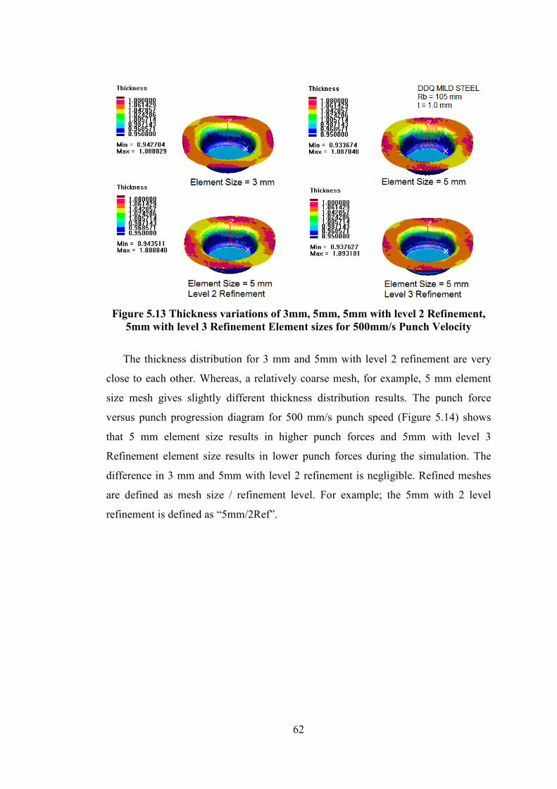
62
Figure 5.13 Thickness variations of 3mm, 5mm, 5mm with level 2 Refinement, 5mm with level 3 Refinement Element sizes for 500mm/s Punch Velocity
The thickness distribution for 3 mm and 5mm with level 2 refinement are very
close to each other. Whereas, a relatively coarse mesh, for example, 5 mm element
size mesh gives slightly different thickness distribution results. The punch force
versus punch progression diagram for 500 mm/s punch speed (Figure 5.14) shows
that 5 mm element size results in higher punch forces and 5mm with level 3
Refinement element size results in lower punch forces during the simulation. The
difference in 3 mm and 5mm with level 2 refinement is negligible. Refined meshes
are defined as mesh size / refinement level. For example; the 5mm with 2 level
refinement is defined as “5mm/2Ref”.

63
Figure 5.14 Punch Force vs. Punch Progression curves for different element sizes
The results for four different element sizes reveal that finer meshes provide
similar results as far as thickness distributions and punch force vs. punch progression
graphs are concerned. The optimization is about obtaining accurate results in
reasonable amount of time. So the comparison of Computational time is investigated
and illustrated in Figure 5.15.
0
5000
10000
15000
20000
3mm 5mm/2ref 5mm/3ref 5mm
Cpu Tim
e (s)
500 mm/s
1000 mm/s
Figure 5.15 Punch Speed and Element size effect on Computational Time
As it can be observed from the figure coarse mesh generates results in small
amount of time compare to finer meshes. However excessive adaptive meshing, like

64
5mm/3Ref, increases Computational time. The important point is adding optimum
level of adaptive meshing to the simulation, finer results can be obtained in smaller
amount of time. 5 mm element sizes are coarse, however by enabling 2 refinement
levels to this mesh, accurate and faster results can be obtained.
All these simulations reveal that adaptive meshing is a powerful tool to establish
a transition between initial and final elements having different lengths during the
simulation, but it should be activated cautiously since unnecessary usage can
significantly increase the computational time.
5.2.4 Mesh Topology
Besides the element size, mesh generation plays a key role in Finite Element
Methods. Different applications require different types of meshing. For example, in
wrinkling analysis radial meshes are preferred. If radial analysis is performed, then
radial mesh is utilized. Tool meshes should be fine in order to avoid penetration
problems and obtain accurate results as stated before. Also, in order to avoid contact
problems, tool meshing and blank meshing should cover each other.
In PAM-STAMP simulations, quadrilateral element type is utilized. Tool and
blank meshing are performed in Marc Mentat and imported to the PAM STAMP. In
order to compare mesh topologies, two different meshes are generated and
simulations are performed. Radial and uniform meshes are shown in Figure 5.16.
Figure 5.16 Uniform and Radial Mesh of the blank

65
The uniform mesh composes of 1460 elements, 1537 nodes and 3012 edges;
however the radial mesh composes of 1945 elements, 1982 nodes and 3926 edges.
Comparing these numbers, one easily state that radial mesh is finer.
If the equivalent plastic strains calculated at the mid-plane of the deformable
bodies are inspected, it can be concluded that minimum strains and maximum strains
are higher for uniform mesh structure compared to radial mesh structure in analysis
of NUMISHEET problem (Figure 5.17). Same difference can be obtained when the
force - displacement curves are observed (Figure 5.18). Forming force requirements
for uniform mesh structure are a little bit higher than for that of radial mesh structure.
According to this fact, it can be stated that although the same material properties are
used in both simulations, using different mesh topologies may influence the stiffness
of the deformable body.
Figure 5.17 Equivalent plastic strain contours of radial and uniform mesh structures

66
Figure 5.18 Punch Force vs. Punch Progression curves for Radial and Uniform mesh structures
For an analysis that targets to investigate the wrinkling phenomenon, radial mesh
structure have advantages over uniform mesh structure. The radial mesh enables the
user to obtain results in cylindrical coordinate system easily. Also, the blankholder
mesh is in radial structure so contact problems are minimized. Another advantage of
radial mesh is wrinkling detection and wrinkled part image is better in radial meshes
(Figure 5.19).
Figure 5.19 Wrinkled blank with uniform and radial mesh structures

67
5.2.5 Comparison with NUMISHEET 2002 Benchmarks
According to the proposed process parameters at Sections 5.2.2, 5.2.3 and 5.2.4 a
cylindrical cup drawing numerical experiment is set up to compare the simulation
results with NUMISHEET 2002 Benchmark in order to verify that those parameters
are optimum and useful for dynamic-explicit finite element codes.
The process setup and geometry of tools used in the benchmark are already
provided in Figure 5.1. In the same setup, steel material with 1 mm thickness is used
as the workpiece. The material data for the workpiece is tabulated in Table 5.1
previously. The radius of workpiece is 105 mm. Same geometrical data is used to
build the meshes in the simulation. Punch speed is chosen as 500 mm/s and punch
stroke is 40 mm. Friction coefficient for all surfaces are stated as 0.0426 by the
material supplier. Blank element size is 3 mm and no refinement is applied. The
uniform mesh is used.
Twenty-three participants have supplied results to NUMISHEET 2002
benchmark. Seven of them have conducted experiments, (Detailed information about
these participants can be found in Appendix A) whereas the rest of them participated
with simulation results obtained from different finite element packages.
The comparison between simulation and benchmark is made by inspecting the
forming force - displacement curves and outer radii of flange. These comparisons are
illustrated in the following figures.

68
Figure 5.20 Comparison of Punch Force – Punch Stroke curve of Pam Stamp simulation with Benchmark Experiments
In Figure 5.20, it can be noticed that the best compliance exists between the
simulation result and AE-04. The results supplied by other participants are slightly
higher than this agreement; however these differences may exist due to the external
influences. For instance, E.H. Atzema (Appendix A) from Corus Research,
Development and Technology has stated that the grid applied to the steel blank
influenced the friction condition, thus it increased the values in the punch force
versus punch displacement graphs by 5 percent. There is a difference of 20 kN in the
measured maximum punch forces between the highest and lowest experimental
findings in Figure 5.20.
Outer profiles of the flange are compared in Figure 5.21 and 5.22 for steel blank
with high blank holder force (HBHF). In Figure 5.21, the outer circumference of
flange is plotted in Cartesian coordinates and in Figure 5.22; it is plotted with respect
to the r and θ in cylindrical coordinates.

69
Figure 5.21 Comparison of outer circumference of steel flanges of Pam Stamp simulation and benchmark experiments
Figure 5.22 Comparison of outer circumference of steel flanges of Pam Stamp simulation and benchmark experiments

70
It is shown that the simulation result only shows some variations from
benchmark experiments AE-02 and AE-07 and is compatible with other three
experiments. The reason of the variation can be the misalignment of the blank
according to the Rolling direction and eccentric placement of blank on the die. In the
simulation such incorrect orientations cannot occur since the recent finite element
codes have features like “auto-positioning”.
Almost all simulation results of steel material are verified with benchmark
experiments. The compliance between the results is not only determined by the
general behavior but also satisfied numerically.
5.3 Wrinkling Simulations
This section is dedicated to the wrinkling phenomenon occur during the deep
drawing process. Flange wrinkling occurs as a result of compressive forces and it is
an undesirable deformation mode. If flange wrinkling occurs during deep drawing
process, the flange region plastically buckles into a number of waves and the process
fails. However, wrinkling can be prevented by the use of blankholder and drawbead.
In the following sections, blankholder and drawbead effects on wrinkling are
discussed.
5.3.1 Blank Holder Simulations
In this section, PAM STAMP simulations with different blank holder forces are
performed and results are discussed. The geometry of the study is again taken from
NUMISHEET 2002 Benchmark, see Figure 5.1. The same material (DDQ Steel) is
used throughout the wrinkling study. Material properties are listed in Table 5.1. The
main objective of this study is to understand the blank holder force effect on
wrinkling instability.
As a starting point in wrinkling analysis, zero blank holder force is used. In other
words, the simulation is performed without a blank holder. After achieving results

71
from blank holder free simulations, many simulations are performed with the same
process parameters except for the applied blank holder force on the blank is
increased.
Throughout the study, in order to comprehend blank holder force effect on
wrinkling, different blank holder forces are applied. Figure 5.23 illustrates deep
drawn part with zero blank holder force.
Figure 5.23 Deep drawn blank without Blank holder
As it can be seen from the Figure 5.23, four waves are formed on the 20 mm
drawn part. In other words, the number of waves formed with zero blank holder force
is four. By increasing the BHF, other results than four waves are obtained. The
different wave formations for 20 mm punch depth with increased blank holder forces
are illustrated in Figure 5.24.
Figure 5.24 Deep drawn parts with different blank holder forces and corresponding wave formations
Figure 5.24 reveals that as the blank holder force increases, wave number
increases and wave amplitude decreases. The wave amplitude in 100 N BHF case is
around 38.3 m whereas this value is 5.5 mm in 3000 N BHF case. Although the wave
amplitude decreases 32.8 mm, the wave number increased to 16 from 4. This effect is

72
also noted by Kaftanoğlu [9]. In the lights of these simulations, it can be stated that;
when a blank holder load is applied to the flange region, wave multiplication occurs
because of that constraint. Also, wave peaks are flattened due to the blank holder
force. The simulations for 20 mm punch progression are tabulated according to the
BHF and corresponding wave number and wave amplitude in Table 5.2.
Table 5.2 Number and Amplitude of Waves for increasing Blank Holder Forces for 20 mm Draw Depth
Blank Holder Force Number of waves Wave amplitude
1 4 38,387
10 4 38,338
100 4 38,305
250 8 36,701
500 8 36,327
1000 10 30,404
2000 14 9,870
3000 16 5,479
4000 16 2,801
Table 5.2 shows simulation results for 20 mm punch depth. For blank holder
forces smaller than 5 kN, severe wrinkling occurs as it can be observed from Figures
5.23-24. These wave amplitudes are getting larger and larger as the punch progress in
to the die. In other words, punch depth affects the flange region wrinkle contour. In
most cases, wave number does not change and wave amplitude increases with the
increasing punch progression.
The punch progression effect on wrinkling is also studied in many simulations.
This study also reveals the wave formation during the process. The blank is viewed
at 1 mm, 5 mm, 10 mm, 15 mm and 20 mm punch depths. The wrinkling wave
formations with the punch progression for different blank holder forces are illustrated
in the Figure 5.25.

73
Figure 5.25 Wave Formations for 1 mm, 5 mm, 10 mm, 15 mm and 20 mm Punch Depths with simulations of 1 N , 1000 N and 3000N Blank Holder Forces
As it can be seen from Figure 5.25, in 1 N blank holder case, the blank starts
wrinkling before 5 mm punch depth and the wave amplitude grows bigger as the
punch progress to 20 mm depth. Wrinkling starts around 10 mm for the 1000 N BHF
case, in other words, the blank does not wrinkle until 10 mm depth is achieved. The
last case shows that 3000 N force applied to the blank hinders the blank from
wrinkling up to 15 mm draw depth.
Since, excessive wrinkling and tearing of waves is observed in flange region for
higher draw depths, the draw depth is kept at 20 mm for low blank holder forces. In
NUMISHEET 2002 Benchmark problem, the draw depth is given as 40 mm. In
wrinkling analysis for blank holder forces higher than 3000 N draw depth is set to 40
mm. Simulations are performed for relatively higher blank holder forces. The main
objective is to achieve the required blankholder force to avoid wrinkling. Blank
holder force is increased up to a point where no waves are seen visually. The
simulation results are tabulated in Table 5.3.

74
Table 5.3 Number and Amplitude of Waves for increasing Blank Holder Forces for 40 mm Draw Depth
Blank Holder Force Number of waves Wave amplitude
4000 16 22,668
5000 16 20,1956
6000 20 4,991
7000 none -
Table 5.3 indicates that with 7000 N blank holder force, the flange region does
not wrinkle. In order to find the exact blank holder force that is required to avoid
wrinkling, further simulations are performed. During these simulations, in order to
find the required blankholder force, binary search algorithm is utilized. In this
algorithm, the next candidate is selected from the arithmetic average of the maximum
and minimum values. So, the first candidate is selected as 6500 N according to the
algorithm. The analysis is performed for 6500 N and flange wrinkling is seen. The
next candidate is selected as 6750 N and flange is wrinkled again. Flange wrinkling
has stopped at 6875 N blank holder force. The study findings are stated in Table 5.4.
Table 5.4 Number and Amplitude of Waves for finding the required Blank Holder Force for 40 mm Draw Depth
Blank Holder Force Number of waves Wave amplitude
6500 24 3,33499
6750 24 2,44956
6875 none -
This study aims to find the required blank holder force in order to avoid
wrinkling. During the study, a relation between the blank holder force and number of
waves formed is discussed. As stated before, the number of waves in the flange
region decreases with the increasing blank holder force. The number of waves
reaches infinity where there is no wrinkling observed. The required blank holder
force restricts these waves to have very little wave amplitudes and as the wave
amplitudes decrease, the flange region remains flat, wrinkle free. Figure 5.26 shows

75
the wave formation for 6500 N, 6750 N and 6875 N blank holder forces. It is noted
that no wrinkling is observed for 6875 N blank holder force.
Figure 5.26 Further analysis images for finding required blankholder force
Figure 5.26 shows that blank holder force restricts the wave formation and at
certain values wave formation in the flange region stops. With 6875 N blank holder
force, flange wrinkling is not observed. While concluding this study, the energy
graphs of these simulations are searched.
If one investigates the wrinkling problem in case of energy graphs of the process,
these graphs show the reason why wrinkling stated as an instability problem in deep
drawing. The energy graphs for different blank holder forces, reveal a very important
issue about wrinkling. As stated before, the material tends to deform in a mode
requiring least energy. In other words, the material tends to wrinkle if the wrinkling
energy is lower than the drawing energy. With the increasing blank holder force,
wrinkling energy also increases so drawing takes place in the blank. The Figure 5.27
shows energy versus punch progression graph for 5000 N blank holder force.

76
Figure 5.27 Energy Graphs for 5000 N Blank Holder Force
In the graph, Kinetic energy and hourglass energy must be small compared to the
external work energy. If these values are high, then this means that the numerical
error of the simulation is high. But in this analysis, both kinetic energy and the
hourglass energy are negligible compared to the external work energy. So the
simulation is safe and correct.
The graph in Figure 5.28 reveals an important point about the wrinkling
instability. In the previous findings, the blank experiences wrinkling in the flange
region for 5000 N blank holder force and the first wave formation for this case takes
place around 25 mm punch progression. The external work graph shows exponential
behavior up to this point and after 25 mm punch progression, the graph looks like a
linear line. This pattern change in the graph suggests that the material deforms in
wrinkling mode. This instability point reveals that wrinkling energy is smaller than
drawing energy and the blank deforms in a mode that requires least energy. The
external energy graph for other blank holder forces are illustrated in Figure 5.28.

77
Figure 5.28 External Energy Graphs versus Punch Progression for 1000 N, 5000 N and 10000 N Blank Holder Forces
As it can be seen from Figure 5.28, the external energies for the three different
blank holder forces are equal up to 12 mm punch progression and then the external
energy for the 1000 N BHF case drops. This is the point when the wrinkling energy
is smaller than the drawing energy and the first waves are formed in the flange
region. The same event can be observed for the 5000 N BHF at around 25 mm punch
progression. However the external energy value for the 10000 N BHF case does not
drop or experience instability. This means, the 10000 BHF is able to avoid wrinkling
in this particular case.
Another important point in wrinkling is the effect of anisotropy. The material is
chosen from NUMISHEET 2002 benchmark as stated before. In order to study the
effect of anisotropy in wave formation in flange region, these analyses are performed
for isotropic material also. All other material properties are taken from the Table 5.1
but material is chosen as isotropic. Figure 5.29 illustrates the effect of anisotropy in
wave formation. The simulations are performed for 1000 N blank holder force with
20 mm punch progression.

78
Figure 5.29 Anisotropic and Isotropic Material wave formations
Although the applied blank holder forces are the same, the anisotropic material
experiences 10 waves, whereas the isotropic has 12 waves as it can be seen from
Figure 5.29. Another important point about the wave formation is wave amplitudes
and wave shapes which are exactly the same in isotropic material case. Also these
waves are symmetric to X and Y planes. On the other hand, the waves formed in the
anisotropic material case show differences and they are not symmetrical. In the light
of these findings, one can state that quarter or half model finite element tools cannot
be used in case of anisotropic material is used. The isotropic model can be solved for
quarter or half model. The number of waves for anisotropic and isotropic material is
illustrated in the Table 5.5.
Anisotropy effect on wave formations is illustrated in Table 5.5. The isotropic
material experiences wave formations that illustrate same amplitude and same shape.
This behavior is expected since the isotropic material does not have any change in
material properties with the direction. The anisotropic material experiences different
wave formations than the isotropic material, can be seen in Table 5.5. In 5000 N
blank holder force case, 16 waves are formed for anisotropic material and 20 waves
are formed for isotropic material.

79
Table 5.5 Number of Waves for Anisotropic and Isotropic Materials
Blank Holder Force Number of waves for
Anisotropic Material
Number of waves for
Isotropic Material
1 4 4
100 4 4
500 8 8
1000 10 12
2000 14 16
3000 16 16
5000 16 20
6000 20 20
6500 24 24
5.3.2 Drawbead Simulations
In this section, PAM STAMP simulations with different drawbead types are
performed and results are discussed. The geometry of the study is again supplied by
NUMISHEET 2002 Benchmark but drawbead models are added to the drawing
process. Same material (DDQ Steel) is used throughout the drawbead study. Material
properties are stated in Table 5.1. The main objective of this study is to understand
the drawbead effect on wrinkling instability. Two types of drawbead are used in this
study, one is the drawbead module available in PAM STAMP program and the other
one is physically designed and utilized drawbead model in the simulations.
There are different drawbead models available in the Pam Stamp program. These
models are taken from Stoughton according to the Reference Manual [20] of the
program. The suitable drawbead models for the Benchmark problem are illustrated in
Figure 5.30.

80
Figure 5.30 Drawbead models of Pam Stamp [20]
Among these drawbead models, the spherical model is not suitable for physical
modeling due to single point contact so the first one is chosen throughout the
drawbead simulations. Although these models represent physical geometries, the
program generates two forces from these models and inputs them to the simulation as
a restraining and opening force (refer to Figure 5.31). Pam Stamp drawbead module
calculates the restraining and the opening forces from the drawbead geometry and
the material properties. The drawbead model is replaced by these forces and in the
real simulation equivalent drawbead are shown in the Figure 5.32. The drawbead
geometry is tabulated in Table 5.6.

81
Figure 5.31 Restraining and Opening Force of the Equivalent Drawbead model
Figure 5.32 Drawbead model in reality and in simulation [20]
Table 5.6 Drawbead geometry parameters
L1 R1 D L2 R2
4 1.5 1.5 6.5 2
The mesh structure of the blank holder and die is not changed by applying this
transformation. This is the main advantage of this drawbead model. Also, this
equivalent drawbead is easier to use. The computation time does not change as the

82
mesh structure remains the same, so as the time step. In addition, the equivalent
drawbead model enables fast responses for drawbead geometry changes, since the
geometry changes do not affect the mesh structure. Also, different drawbead
geometries can be easily implemented to the system and simulated.
The groove depth, D (refer to Figure 5.30), effect on the deep drawing process is
investigated for different depth values. All the other dimensions are kept constant
except for groove depth. Figure 5.33 shows thickness distribution for 1.5 mm, 2.0
mm and 2.5 mm groove depths.
Figure 5.33 Thickness distributions for 1.5 mm, 2.0 mm and 2.5 mm groove depths at 20 mm punch depth
The groove depth is very effective in material flow as it can be seen from Figure
5.33. 2.0 mm and 2.5 mm groove depths result in excessive thinning at the bottom of
the cup. Thickness of the blank reduces 20 percent for 2.0 mm groove and 40 percent
for 2.5 mm groove. The thickness distribution in the flange region is similar for all
different groove values. Also, wrinkling is avoided for all these cases.
In order to understand drawbead effect on wrinkling many simulations are
performed. Simulations aim to locate the most effective drawbead in avoiding the
wrinkling. Three different drawbead radii are studied; the radii of these models are
70mm, 80 mm and 90 mm. The drawbead radii and their positions on the die

83
blankholder set are shown in Figure 5.34. The drawbead models are represented as
purple circles in the simulation. Thickness contours for these drawbead models with
1.5 mm groove depth for 20 mm punch depth is illustrated in Figure 5.35.
Figure 5.34 Drawbead models for 70 mm, 80 mm and 90 mm
Figure 5.35 Thickness contours for 70 mm, 80 mm and 90 mm radii drawbeads
Thickness contours of these different drawbead analyses are very close to each
other as it can be derived from Figure 5.35. The thickness values at the bottom of the
cups are very similar in magnitude. However, the thickness distribution in the flange
region experiences some difference with drawbead size. Flange thickness of the 70
mm radius drawbead model seems to have a uniform distribution. The other

84
drawbeads do not show this uniform thickness in the flange region. In all drawbead
analyses, the flange region between drawbead location and the outer diameter of the
blank experiences uniform thickness distribution as it can be seen from Figure 5.35.
In order to obtain uniform distribution drawbeads, one shall use 70 mm radius
drawbead model, nearest possible drawbead model to the center.
Same drawbead geometries are used in the simulations for these three different
drawbead radii. After the further simulations 90 mm model seems to be the least
effective, because the drawbead do not cover the blank as it flows into the die.
Anisotropy of the material is the main reason that the drawn part deviates from its
circular shape as it can be seen from the Figure 5.36.
Figure 5.36 Fully drawn part with 90 mm drawbead
In simulations, same blank holder forces are used for both drawbead models.
While using same blank holder forces, the most important point is to comprehend the
effect of opening force, because when the opening force is higher than the blank
holder, the wrinkling analysis will be meaningless physically. Opening force
increases as the groove depth increases, so the needed blank holder force increases.
Figure 5.37 shows that the blank experiences severe wrinkling when opening force
beats blank holder force.

85
Figure 5.37 Wrinkled blank due to insufficient blank holder force
The drawbead study is continued with the physical modeling of the drawbead in
the simulation. The meshing of this study is also performed by using Marc Mentat.
The blank holder and the die geometries are meshed again with the physical
drawbead geometries. The geometry of the drawbead is illustrated in Figure 5.38.
Figure 5.38 Drawbead Geometry for small and large groove [20]
Two different geometries are used for small and large grooves. Geometrical
properties of both small and large grooves are tabulated in Table 5.7 and all
dimensions are given in milimeters. Figure 5.39 illustrates simulation models with
these drawbead models.
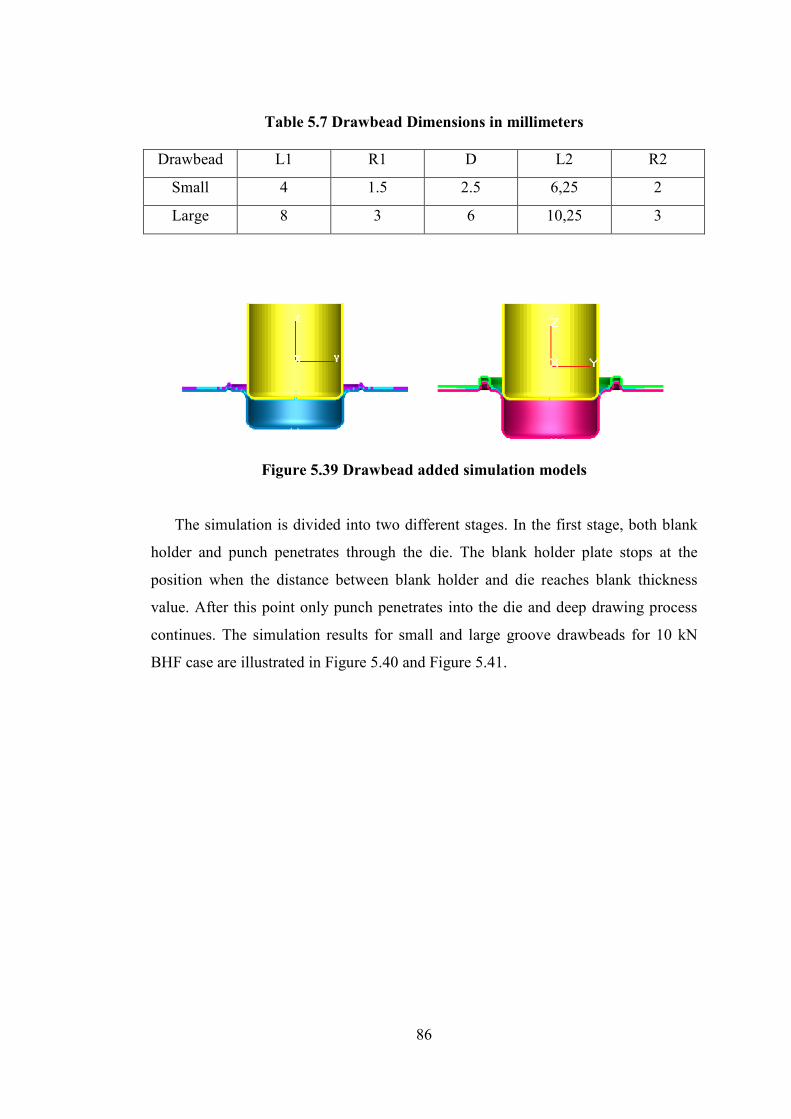
86
Table 5.7 Drawbead Dimensions in millimeters
Drawbead L1 R1 D L2 R2
Small 4 1.5 2.5 6,25 2
Large 8 3 6 10,25 3
Figure 5.39 Drawbead added simulation models
The simulation is divided into two different stages. In the first stage, both blank
holder and punch penetrates through the die. The blank holder plate stops at the
position when the distance between blank holder and die reaches blank thickness
value. After this point only punch penetrates into the die and deep drawing process
continues. The simulation results for small and large groove drawbeads for 10 kN
BHF case are illustrated in Figure 5.40 and Figure 5.41.

87
Figure 5.40 Small drawbead analyses for 10 kN BHF
In Figure 5.40, the flange region experiences wrinkling at 20 mm punch
progression. The applied blank holder load does not prevent wrinkling, so a higher
blank holder force should be used. Thickness values at 0 mm indicate that the
material is thinned as it is shaped by drawbead model. As the punch progresses into
the die, thickness at the bottom of the blank experiences more and more thinning.
The thickness values near punch fillet radius are lowest and there may be a possible
tearing if punch progresses more. The minimum thickness value is around 0.9 mm
and the maximum is around 1.05 mm.

88
Figure 5.41 Large drawbead analyses for 10 kN BHF
Figure 5.41 shows that the blank experiences wrinkling just similar to small
drawbead model. The BHF is not enough to hinder wrinkling. The thickness values
at 0 mm punch progression are lower than small drawbead case, which is expected as
the groove depth is larger when larger drawbeads are used. The minimum thickness
values are around 0.93 mm in small drawbead case whereas it is around 0.91 mm for
large drawbead case. The minimum thickness value at 20 mm punch progression is
around 0.89 mm, which is lower than the thickness value of small drawbead case. As
both small and large drawbead simulations experience wrinkling, higher BHF is
used. The simulation results for small and large groove drawbeads for 100 kN BHF
case are illustrated in Figure 5.42 and Figure 5.43.
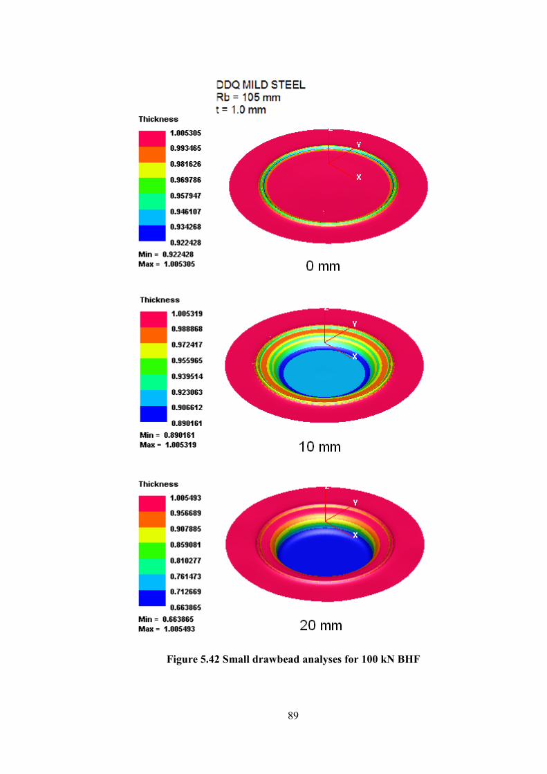
89
Figure 5.42 Small drawbead analyses for 100 kN BHF

90
Figure 5.43 Large drawbead analyses for 100 kN BHF

91
Figure 5.42 and 5.43 indicate that higher blank holder force (100 kN) eliminates
the wrinkling problem, however the blank experiences excessive thinning. The blank
thickness decreases to 0.66 mm for small drawbead and to 0.64 mm for large
drawbead. Wrinkling problem is eliminated, however tearing problem is observed.
As the material flow in to the die decreases, more and more thinning is observed. In
order to obtain wrinkle and necking free final part, more smooth material flow is
utilized by using inclined drawbead model.
The inclined model is designed in order to enable more material flow into the die.
The inclined drawbead model dimensions are given in Figure 5.44. In the small and
large groove models, the material flow into the die is poor and this yields to tearing
at the bottom of the drawn part. The inclined drawbead model aims to achieve good
material flow and less thinning in the blank, the results are satisfactory as can be seen
from Figure 5.45.
Figure 5.44 Inclined drawbead dimensions

92
Figure 5.45 Thickness contours for inclined drawbead model with 100 kN BHF

93
Figure 5.45 shows that the blank does not wrinkle in the flange region, similar to
previous drawbead models. The blank thickness at the bottom region is around 0.79
mm that indicates the blank experiences less thinning than the other drawbead
models. The material flow for inclined model is smoother and easier as expected.
The physical modeling of the drawbead is very difficult and time consuming. The
first problem is encountered in meshing. The drawbead size is very small compared
to the blank size. Small size drawbead results in small sized elements in contact
region of the blank and drawbead model. So, in order to obtain good contact region;
level 5 (highest level available in the program) adaptive meshing is used in
simulations. This excessive refinement results in a very sharp increase in
computation time. The mesh structure before and after the simulation is illustrated in
Figure 5.46.
Figure 5.46 Mesh structure before and after the simulation
Energy graphs of the drawbead simulations are illustrated in Figure 5.47. Small,
large and inclined drawbead models result in different punch progression vs. external
work diagrams. The inclined model energy is higher than the other two drawbead
models.

94
Figure 5.47 External energy diagrams for different drawbead models
5.4 Experimental Study
This section is dedicated to the experimental study performed. The aim of this
study is to understand the effect of thickness in wrinkling problem. In order to study
thickness effect, four different sheets with the same material, AL 1050, are used. The
thickness values for this experiment are chosen as 0.5 mm, 1.0 mm, 1.2 mm and 2.0
mm. In order to obtain the material properties for these four set of materials, tension
test is performed. After obtaining the material properties, deep drawing experiment is
conducted. The wrinkling behavior for different thicknesses is studied and the finite
element modeling of the experiment is performed. The simulation and the
experimental findings are compared.
5.4.1 Tension Test
There are four sheet blanks used in this study. In order to find the material
properties, tension tests are conducted. The required material properties are found by
conducting tension tests at Metal Forming Centre of Excellence in Atılım University.

95
The experiment specimens are prepared and the test is conducted for four different
thicknesses of Al 1050. For one set of tests, 9 specimens are prepared, a total of 36
specimens are used in the experiment. In order to find anisotropy constants, the
specimens are cut according to the rolling directions of the sheet material. For one
test in 0, 45 and 90 degrees according to the rolling direction, 3 specimens are
subjected to tension and the results are obtained. These results are processed by the
software available in the test setup and the material properties are calculated
accordingly. The test setup is illustrated in Figure 5.48. The test specimens before
and after the tension test are shown in Figure 5.49.
During the tension test, all data are obtained and processed in the available
software program of the Zwick Test setup. The tension test is performed according to
the ISO 10113,05/1991 and ISO 10275,02/1993. These standards cover tensile tests
on metals with determination of the vertical anisotropy and the hardening exponents.
The tension test results are illustrated in Table 5.8.
Figure 5.48 Universal Tensile Testing Machine with 30 ton force capacity (Zwick)

96
Figure 5.49 Tension Test specimens, 2 mm thickness, before and after the test
Table 5.8 Material Properties of AL 1050 Material for four thickness values
Material E
(GPa)
ρρρρ
(g/cm3) νννν
K
(MPa) n
R
(0°)
R
(45°)
R
(90°)
Al 1050 0.5 mm 59,133 2,7 0,33 99,847 0,1196 0,637 0,496 0,578
Al 1050 1.0 mm 59,766 2,7 0,33 140,86 0,0872 0,896 0,611 0,660
Al 1050 1.2 mm 58,888 2,7 0,33 162,33 0,0963 0,652 0,751 0,684
Al 1050 2.0 mm 57,944 2,7 0,33 286,28 0,0976 0,681 0,833 0,803
5.4.2 Conventional Deep Drawing Experiment
There are three different sizes of sheet blanks with four different thicknesses are
used in this study. The diameters of the blanks are 80mm, 90mm and 100mm. In
order to understand the thickness effect on wrinkling, conventional deep drawing
experiments are conducted. These experiments are conducted at Metal Forming
Laboratory of METU. In the experiments Tinius Olsen Testing Machine is used. This
testing setup has lots of deep drawing tools available. From these tools, the most
applicable punch and die set is selected. The punch diameter is chosen as 50 mm and
the die diameter is 54 mm. The fillet radii of punch and die are 5 mm. During the
experiment, 0.5 mm, 1.0 mm, 1.2 mm and 2.0 mm thickness sheets are used. Grease
is used as a lubricant throughout the experiment. Average coulomb friction
coefficient at all contact surfaces are assumed as 0.08. The friction coefficient value
is taken from the previous work of Kaftanoğlu [9]. In order to obtain zero blank

97
holder force, four nuts are placed around the blank between the die and blank holder.
Without blankholder force, the wrinkling in the flange region takes place freely. At
first steps, free wrinkling is observed but when the wave amplitudes become higher
than the nut height due to increased punch depth, blank holder force is applied to the
blank. Tinius Olsen testing machine is illustrated in Figure 5.50. The specifications
of the testing machine are given in Appendix B.
Figure 5.50 Tinius Olsen Tesing Machine
The deep drawn parts with different thickness values and different diameter sizes
are illustrated in Figure 5.51.

98
Figure 5.51 Deep Drawn parts with different thickness and different diameters
In Figure 5.51, all of the test specimens are illustrated. The wrinkle wave
formations show significant differences for different thickness values. The diameter
for the first specimen set is chosen as 80 mm. The thickness effect on the wrinkle
formation for 80 mm diameter set can be seen in Figure 5.52.
Figure 5.52 Wrinkling formations for 80 mm diameter blanks

99
It can be seen clearly from Figure 5.52 that, the wave number decreases as the
thickness of the blank increases. 0.5 mm thick part experiences 8 waves with high
wave amplitudes but the 2.0 mm thick part does not wrinkle. Figure 5.53 shows the
wrinkling formations for 100 mm diameter blanks.
Figure 5.53 Wrinkling formations for 100 mm diameter blanks
Similarly for the 100 mm blank, the wave number decreases as the thickness of
the blank increases. 0.5 mm thick part experiences 5 waves with high wave
amplitudes but the 2.0 mm thick part have 2 shallow waves.
In order to verify the simulation results of PAM STAMP program, this
experiment is simulated and the results are compared. The simulations are performed
according to the material properties obtained in Tension tests. The experimental
setup is modeled and the blanks with different sizes and thicknesses are meshed. The
process parameters are obtained from the conventional deep drawing experiment.
The punch progression values for each diameter sets are different in the experiment.
Therefore, in the simulation highest value is selected and the process is divided into
many steps. By doing this kind of regulations in the simulations, one can obtain the
wave formation progress with respect to the punch progression. The experimental
setup, modeled in PAM STAMP, is illustrated in Figure 5.54 and the deep drawn part
in experiment and simulation is shown in Figure 5.55.

100
Figure 5.54 Finite Element Model of the experiment tools
Figure 5.55 Experimented and Simulated deep drawn part
Simulation results for 80 mm, 90 mm and 100 mm diameter blanks are illustrated
in Figure 5.56, 5.57 and 5.58, respectively. In these simulations, blank holder force is
set to 0 N. Table 5.9 summarizes experiment and simulation results.
Figure 5.56 Wrinkling formations for 80 mm diameter blanks

101
Figure 5.57 Wrinkling formations for 90 mm diameter blanks
Figure 5.58 Wrinkling formations for 100 mm diameter blanks
Table 5.9 Experiment and Simulation results for specified blank diameters with different thicknesses
Experiment Results Simulation Results
Number of Wave Number of Wave Blank
Diameter 0.5 1.0 1.2 2.0 0.5 1.0 1.2 2.0
80 mm 10 8 8 - 8-10 8 8 -
90 mm 8 4 4 4 8 6 4 4
100 mm 5-7 4 4 2 6 4 4 4
Experiment and simulation results are in good correlation with each other.
Results also indicate that wrinkling is a more serious problem for thinner materials.
Thinner materials have higher tendencies to plastic wrinkling.

102
CHAPTER 6
DISCUSSION
In this study, a commercial dynamic – explicit finite element program PAM
STAMP is used in order to analyze the wrinkling behavior in deep drawing
processes. The NUMISHEET 2002 benchmark problem is selected to verify the
finite element program reliability. The process parameters of the program are
inspected thoroughly in order to complete an optimization analysis.
The effect of punch velocity on simulation is inspected by trying various punch
velocities, a wide range from 50 mm\s to 50000 mm\s. These effects are compared
according to the accuracy of the results and the computational time. According to
these analyses, computational time increases so much for punch speeds lower than
250 mm/s and the accuracy of the results are not satisfying for punch speeds higher
than 10000 mm/s, see Figure 5.6 and Figure 5.7. The other process parameters are
element size and refinement. From these analyses, the mesh must be fine in order to
obtain reliable results. The refinement is a powerful tool that enables the mesh to be
finer wherever necessary and optimum refinement enhances the mesh quality without
increasing computational time. Thickness distribution graph (Figure 5.13) indicates
that thickness variations, maximum and minimum thicknesses are very close, almost
same, for 3 mm element size and 5 mm element size with 2 refinement levels.
Simulations for 500 mm\s punch velocity (Figure 5.15) indicates that computational
time for 3 mm element size is around 3 hours and for 5 mm element size with 2
refinement level is around 2.5 hours. Another important parameter is mesh topology.
Figure 5.17 illustrates that, minimum strains are obtained as 0.0158 for radial mesh
and 0.0293 for uniform mesh and maximum strains are obtained as 0.481 for radial
mesh and 0.493 for uniform mesh. Figure 5.18 illustrates that forming force
requirements for uniform mesh structure are nearly %10 higher than for that of radial

103
mesh structure. It can be stated that although the same material properties are used in
both simulations, using different mesh topologies may influence the stiffness of the
deformable body. The radial mesh topology seems to give more reliable results for
wrinkling analysis. Also, radial mesh is more suitable to wrinkling analysis.
The simulation results of NUMISHEET 2002 benchmark problem are compared
with experimental data given from the participants. Throughout this study, 500 mm\s
punch velocity, uniform mesh with 3 mm element size and no mesh refinement are
selected as process parameters. Punch force vs. Punch progression graph (Figure
5.20) shows that the simulation results are very close to experimental data, AE-04.
The results supplied by other participants are slightly higher (around %15) than this
agreement. There is a difference of 20 kN in the measured maximum punch forces
between the highest and lowest experimental findings in Figure 5.20. However these
differences may exist due to the external influences. For instance, E.H. Atzema
(Table A.7) from Corus Research, Development and Technology has stated that the
grid applied to blank influenced the friction condition, thus it increased the values in
the punch force versus punch displacement graphs by 5 percent. The general trend
line for the simulation and experimental findings are in good correlation. The
analysis in cylindrical coordinates shows that outer flange contours of the simulation
are very close to the experimental findings (Figure 5.21). However the analysis
shows that some of the experimental data are not reliable and suitable because they
supply low number of data points. Also, the experiment data shows that there is a
wide variation in the experimental results. This variation can be related with the
quality of the tools used and the precision of the experiment and measurement. The
specified lubrication conditions may not be satisfied from the participants so the
experiment results show some differences. The misalignment of the blank into the
punch die set may be another reason for this unreliable experiment results.
The blank holder simulations are performed for the same geometry of benchmark
problem. Blank holder forces from 0 N to 10000 N are simulated. The simulations
show that the blank experiences 4 waves in the flange region for zero blank holder
force. The blank holder force analysis reveals that as the blank holder force

104
increases, the wave number increases and the wave amplitude decreases. Table 5.2
illustrates results for 20 mm draw depth from 1 N to 4000 N blank holder forces.
Wave amplitude for 1 N blank holder force is around 38.4 mm, and this value
decreases to 2.8 mm for 4000 N. This expected behavior continues up to a point
where wrinkling of the flange stops. In other words, the amplitude of the waves
decreases to zero. The results show that 6875 N blank holder force is required to
eliminate wrinkling for isotropic material case. In this study, wave numbers at the
flange region starts from 4 and increases up to 24 waves for 6500 N and 6750 N
blank holder forces. The punch progression effect on wrinkling (Figure 5.25) also
observed. In the free wrinkling case the blank starts wrinkling before 5 mm punch
depth and the wrinkling starts around 10 mm for 1000 N blank holder force case. The
last case shows that 3000 N force applied to the blank hinders the blank from
wrinkling up to 15 mm draw depth. It can be stated that, 7000 N blank holder force
avoids wrinkling in flange region for only 40 mm punch progression.
Deep drawing energies for 1000 N, 5000 N and 10000 N blank holder forces
(Figure 5.28) equal up to 12 mm punch progression and then the deep drawing
energy for the 1000 N BHF case drops. This is the point where the wrinkling energy
is smaller than the drawing energy and waves are formed in the flange region. The
same event can be observed for the 5000 N BHF at around 25 mm punch
progression. These instability points reveal that wrinkling energy is smaller than
drawing energy for 1000 N and 5000 N blank holder forces. The material deforms in
wrinkling mode, because the blank deforms in a mode that requires least energy in
deep drawing processes. However the deep drawing energy for the 10000 N BHF
case does not drop or experience instability. This means, the 10000 BHF is able to
avoid wrinkling in this particular case. Also, the anisotropy effect on wrinkling is
discussed. Although the applied blank holder forces (1000 N) are the same, the
anisotropic material experiences 10 waves, whereas the isotropic has 12 waves, refer
to Figure 5.29. The flange region for isotropic case experiences 4, 8, 12, 16, 20 and
24 waves for a range of 1 N – 6500 N blank holder forces. The wave numbers are
multiples of four and wave amplitudes are same for all waves of isotropic material
case.

105
Drawbead analysis starts with implementing available drawbead models of PAM
STAMP. The groove depth is very effective in material flow, refer to Figure 5.33. 2.0
mm and 2.5 mm groove depths result in excessive thinning at the bottom of the cup.
Thickness of the blank reduces 20 percent for 2.0 mm groove and 40 percent for 2.5
mm groove. 70 mm, 80 mm and 90 mm radii drawbead locations are used to locate
the most effective drawbead position. The drawbead radius of 90 mm is not used
after first simulations because the drawbead does not cover the blank as it flows into
the die. After comparing wrinkling behaviors (Figure 5.35) for available drawbead
locations, the 70 mm radius drawbead model gives better wrinkling prevention and
uniform thickness distribution in the flange region. Drawbead module of PAM
STAMP is easy to implement, enables fast responses for drawbead geometry changes
and is very suitable for pre-design studies of drawbead design.
Physical models of the drawbeads are meshed into the blank holder and die. For
10 kN blank holder forces, both small and large drawbead model experiences
wrinkling at the flange region. In order to obtain wrinkle free final product higher
blank holder force (100 kN) is applied in the process. The analyses for small and
large drawbead models for 100 kN blank holder force show that wrinkling is
prevented but, drawbead contour does not enable material flow into the die and
behaves like a lock bead (Figure 5.42 and Figure 5.43). The blank thickness contour
shows that excessive thinning is experienced in the bottom part of the blank.
Minimum thickness is 0.663 mm for small drawbead and 0.641 mm for large
drawbead models. Possible tearing may take place for 100 kN blank holder force. In
order to improve material flow into the die, inclined model is designed and
simulations are performed. The results (refer to Figure 5.45) show that inclined
model enables better material flow into the die, which results in less thinning in the
blank. The minimum thickness of the blank is improved to 0.79 mm; this indicates
%20 improvement in material flow. Wrinkling and necking for blank is prevented for
100 kN blank holder force with inclined drawbead model.
Experimental findings of the conventional deep drawing reveal that the wrinkling
is an important problem for thinner blanks. The wrinkling behavior increases as the

106
thickness of the blank decreases, this is expected. Both experiment and simulation
results indicates that, 80 mm diameter blank with 0.5 mm thickness experiences 10
wrinkle waves but no waves are formed for 2.0 mm blank thickness case. 100 mm
diameter blank with 0.5 mm thickness experiences 5 - 7 waves in the experiment and
the simulation indicates 6 waves for this case. The simulations and experiments show
that as the thickness decreases the material is more likely to experience wrinkling.
Also, Table 5.9 indicates that blank diameter affects the number of waves formed. As
the blank diameter is increased, number of waves formed at the flange region
decreases. With 0.5 mm blank thickness; 10 waves are formed for 100 mm diameter
blank, 8 waves are formed for 90 mm diameter and 5-7 waves are formed for 100
mm diameter blank. More waves are formed at the flange for the smallest diameter
blank (80 mm) case. To conclude, experiment results are in good correlation with the
simulation results.

107
CHAPTER 7
CONCLUSION
In this study, the commercial finite element program PAM STAMP is utilized for
modeling of plastic wrinkling in deep drawing. Tool geometries and material
properties are supplied from NUMISHEET 2002 Benchmark. FE program
parameters and their effects on the results are discussed and the optimization study is
performed. The parameter effects on accuracy of the results and computational time
are compared and the optimum parameters are selected accordingly. FE results are
compared with experimental findings (Figure 5.20-5.22) of the benchmark, and the
reliability of the dynamic – explicit finite element code is verified.
The effect of blank holder force on wrinkling is inspected for deep drawing
quality steel material. Plastic work diagrams for 1000 N, 5000 N and 10000 N blank
holder forces are illustrated (Figure 5.28) and wrinkling instability concept is
discussed. Moreover, drawbead models are implemented to the problem and results
are illustrated. Drawbead effect on wrinkling prevention is discussed. Finally, blank
thickness effect on wrinkling is studied both experimentally and numerically. The
material properties for 0.5 mm, 1.0 mm, 1.2 mm and 2.0 mm thicknesses of hard
aluminum are found by conducting tension tests. Conventional deep drawing
experiments for 80 mm, 90 mm and 100 mm diameter blanks of 0.5 mm, 1.0 mm, 1.2
mm and 2.0 mm thicknesses are performed. The experiment data and simulation data
are compared and discussed. In conclusion, following general results have been
obtained with respect to finite element simulations and experiments:
• Blank holder forces from 0 N to 10000 N are simulated for 1 mm
thickness quality steel material. For 0 N blank holder force 4 waves are
observed in the flange region (Table 5.2). After performing simulations, it
108
is found that in order to prevent wrinkling 6875 N blank holder force is
required.
• The blank holder force analysis reveals that as the blank holder force
increases, the wave number increases and the wave amplitude decreases.
Table 5.2 illustrates results for 20 mm draw depth from 1 N to 4000 N
blank holder forces. Wave amplitude for 1 N blank holder force is around
38.4 mm, and this value decreases to 2.8 mm for 4000 N.
• In this study, wave numbers at the flange region starts from 4 and
increases up to a maximum of 24 waves for 6500 N and 6750 N blank
holder forces.
• Deep drawing energies for 1000 N, 5000 N and 10000 N blank holder
forces (Figure 5.28) equal up to 12 mm punch progression and then the
plastic work for the 1000 N BHF case drops. Plastic wrinkling is observed
at the flange region. This instability point reveals that wrinkling energy is
smaller than drawing energy.
• Instability point for the 5000 N BHF can be observed at around 25 mm
punch progression. Again wrinkling energy is smaller than drawing
energy and blank deforms in a mode that requires least energy, as it is
also stated by Kaftanoğlu [9].
• It is observed that the energy of wrinkling increases as blank holder force
increases. After applying required blank holder force, wrinkling does not
occur since it requires a greater energy than drawing. Deep drawing
energy trend line is illustrated as 10000 N Blank holder force case in
Figure 5.28.
• Drawbead module of PAM STAMP is utilized in pre-designing of
drawbead models. Different groove depths and drawbead locations are
compared. It is found that FE drawbead module is easy to implement and
enables fast responses for drawbead geometry changes.
• Simulations for small and large drawbead models for 10 kN and 100 kN
blank holder force reveals that these drawbead models are not suitable for
preventing wrinkling and necking (Figure 5.40-5.43).

109
• In order to improve material flow into the die, inclined model is designed
and simulations are performed. The results (refer to Figure 5.45) show
that inclined model improves material flow by %20. Wrinkling and
necking for blank is prevented for 100 kN blank holder force with
inclined drawbead model.
• Experimental findings of the conventional deep drawing reveal that the
wrinkling is an important problem for thinner blanks. Both experiment
and simulation results indicates that, 80 mm diameter blank with 0.5 mm
thickness experiences 10 wrinkle waves but no waves are formed for 2.0
mm blank thickness case (Table 5.9). The simulations and experiments
show that as the thickness decreases the material is more likely to
experience wrinkling.
• Both experiment and simulation results indicate that, as the blank
diameter is increased, number of waves formed at the flange region
decreases. With 0.5 mm blank thickness; 10 waves are formed for 100
mm diameter blank, 8 waves are formed for 90 mm diameter and 5-7
waves are formed for 100 mm diameter blank.
• It can be concluded from Table 5.9 that, experiment results are in good
correlation with the simulation results.
As a conclusion, this study is expected to be valuable for understanding deep
drawing process and plastic wrinkling problem. The simulations performed and the
experiments conducted enlighten nearly every aspect in understanding wrinkling and
its prevention.

110
REFERENCES
1. Johnson W., Mellor P.B., “Engineering Plasticity”, Ellis Horwood Ltd., 1983.
2. Grote K.-H., Antonsson E.K., “Springer Handbook of Mechanical
Engineering”, 2008.
3. http://www.custompartnet.com/wu/sheet-metal-forming, last accessed; 15th
August 2010.
4. Metal Forming Handbook, Schuler, Springer-Verlag, Berlin Heidelberg,
1998.
5. M. Colgan, John M.: Deep Drawing Process, Journal of Material Processing
Technology, 2003.
6. K. Siegert, S. Wagner, “TALAT Lecture Deep Drawing”, 1994.
7. Serope K., Steven R.S., “Manufacturing Engineering & Technology”, 2006.
8. Banabic, D.; Bunge, H.-J; Pöhlandt, K.; Tekkaya, A. E.: Formability of
Metallic Materials, Springer-Verlag: Berlin/Heidelberg/New York/Tokyo,
2000.
9. Kaftanoğlu B., “Plastic Analysis of Flange Wrinkling in Axisymmetrical
Deep Drawing”. Proceedings of the 21st International Machine Tool Design
and Research Conference, 1980, pp.21–28.
10. Ramaekers J.A.H, de Winter A., Kessels M.W.H., “”Deepdrawability of a
Round Cylindrical Cup”, IDDRG’94, 1994, pp.403–412.

111
11. Cao J., Boyce M.C., “A Predictive Tool for Delaying Wrinkling and Tearing
Failures in Sheet Metal Forming”, Transactions of the ASME, Vol.119,
October 1997, pp.354–365.
12. Cao J.,”Prediction of Plastic Wrinkling Using the Energy Method”, Journal of
Applied Mechanics, Vol.66, September 1999, pp.646–652.
13. Alves J.L., Oliveira M.C., Menezes L.F., “Study of the Influence of the
Refinement of a 3–D Finite Element Mesh in Draw–In Ears and Wrinkles of
a Deep Drawn Cylindrical Cup”, Proceedings of the 5th International
Conference and Workshop on Numerical Simulation of 3D Sheet Forming
Processes, Vol.1, 2002, pp.301–306.
14. Nakamura Y., Ohata T., Nakamachi E., Katayama T., Ueda T., “Study of
Optimum Drawbead Design in Sheet Metal Forming”, Proceedings of the 5th
International Conference and Workshop on Numerical Simulation of 3D
Sheet Forming Processes, Vol.1, 2002, pp.585–590.
15. Zeng X.M., Mahdavian S.M., “Critical Conditions of Wrinkling in Deep
Drawing at Elevated Temperature”, Journal of Materials Processing
Technology, Vol.84, 1998, pp.38–46.
16. Önder İ.E, “Assessment of sheet metal forming processes by numerical
experiments”, Ph.D Thesis, Middle East Technical University, Mechanical
Engineering Department, Ankara, May 2005.
17. Sönmez Ç., “Investigation of the deep drawability of steel and aluminum
sheets by finite element simulation”, Ph.D Thesis, Middle East Technical
University, Mechanical Engineering Department, Ankara, April 2005.

112
18. A. E. Tekkaya: Finite Element Analysis in Solid Mechanics, Lecture Notes,
Middle East Technical University, Ankara, 2002
19. K. Schewizerhof, J.O. Hallquist: Explicit Integration Scheme and Contact
Formulation for Thin Sheet Metal Forming In: FE-Simulation of 3D sheet
metal forming processes in automotive industry. VDI-Ber. 894 (1991), 405 –
439.
20. PAM-STAMP 2G Reference Manual, ESI-Software, France, October, 2002.
21. PAM-STAMP 2G User’s Guide, ESI-Software, France, October, 2002.
22. NUMISHEET 2002 Benchmark A: Deep Drawing of Cylindrical Cup,
NUMISHEET 2002, Proceedings of the Fifth International Conference and
Workshop on Numerical Simulation of 3D Sheet Forming Processes, Jeju
Island, Korea, October 21-25, 2002.

113
APPENDIX A
NUNMISHEET 2002 BENCHMARK PARTICIPANTS
Table A.1 Participant information of AE-01
Experiment AE-01
Benchmark participant: Haruyuki Konishi (Kobe Steel), Robert E
Dick(ALCOA)
Address: 5-5 Takatsukadai 1, Nishi-ku, Kobe, 651-2271
JAPAN
Email: [email protected], [email protected]
Phone Number: 81-78-992-5515
Fax Number: 81-78-992-5517
Table A.2 Participant information of AE-02
Experiment AE-02
Benchmark participant:
Address:
Email:
Phone Number:
Fax Number:
No data is provided for this participant and
benchmark experiment
Table A.3 Participant information of AE-03
Experiment AE-03
Benchmark participant: L. Filice
Affiliation: University of Calabria
Address: Dep. of Mech. Eng. , 87036 RENDE (CS) - Italy
Email: [email protected]
Phone Number: +39 0984 494608
Fax Number: +39 0984 494673

114
Table A.4 Participant information of AE-04
Experiment AE-04
Benchmark participant: Joachim Danckert
Affiliation: Department of Production, Aalborg University
Address: Fibigerstraede 16, DK-9220 Aalborg, Denmark
Email: [email protected]
Phone number: 45 9635 8959
Fax number: 45 98 15 30 30
Table A.5 Participant information of AE-05
Experiment AE-05
Benchmark participant: P.P. Date, Amit. M. Joshi, V. Anil Kumar. Sammeta
Affiliation: Indian Institute of Technology, Bombay
Address: Mech. Eng. Dept. IIT. Bombay, Powai, Mumbai-
India
Email: [email protected], [email protected]
Phone number: 91 22 576 7511
Fax number: 91 22 572 6875
Table A.6 Participant information of AE-06
Experiment AE-06
Benchmark participant: Jonathan White*, Seung-Geun Lee*, Y.Choi*, J.K.Lee*, R.H. Wagoner**
Affiliation: The Ohio State University, *Dept. Mech. Eng., **Dept. Mat. Sci. and Eng.
Address: *209 West 18th Avenue. Columbus Ohio 43210 **2041 College Drive, Columbus Ohio 43210
Email: [email protected], [email protected]
Phone number: (614)292-7371
Fax number: (614)292-7369
Remarks: All measurements are numerical averaged values of three experiments

115
Table A.7 Participant information of AE-07
Experiment AE-07
Benchmark participant: E.H. Atzema
Affiliation: Corus Research, development & Technology
Address: IJTC-PRA-AUT-STP
Email: 3H36 / 1-18; P.O. Box 10.000; 1970 CA IJmuiden; Netherlands
Phone number: +31 2514 98524'
Fax number: +31 2514 70432'
Remarks:
Thickness was obtained from optical surface strain measurements (PHAST tm) on the outside surface of the cup. This means the strains will be over estimated and consequently the thickness underestimated at the punch radius. The other way around at the die radius. Moreover the grid applied may influence the friction. On the aluminum the grid showed no influence on force displacement diagram, on steel a 5% increase in force was seen.

116
APPENDIX B
TINIUS OLSEN TESTING MACHINE
Table B.1 Specifications of Tinius Olsen A-40 Testing Machine
Model A-40
Maximum Capacity 70000 Ibs.
Low Range Capacity 30000 Ibs.
Maximum Diameter Cup 75 mm
Clamping Pressure 0-20000 Ibs.
Testing Speed 0-12 inch/min
Stroke 0-3 inch
Motor Horsepower 3
Width 28 inch
Depth 27 inch
Height 72 inch
Net Weight 1480 Ibs.
Gross Weight 1820 Ibs.