Embed Size (px)
Citation preview
ANALYSIS AND MODELLING OF A NOVEL APPROACH FOR THE INTERROGATION UNIT OF FIBER BRAGG GRATING SENSORS USING
OPTICAL FREQUENCY DOMAIN REFLECTOMETRY TECHNIQUES
A Thesis Submitted to the Graduate School of Engineering and Sciences of
İzmir Institute of Technology in Partial Fulfillment of the Requirements for the Degree of
MASTER OF SCIENCE
in Electronics and Communication Engineering
by Deniz PALA
July 2014 İZMİR
We approve the thesis of Deniz PALA Examining Committee Members: Assist. Prof. Dr. Kıvılcım YÜKSEL ALDOĞAN Department of Electrical and Electronics Engineering Izmir Institute of Technology Prof. Dr. M. Salih DİNLEYİCİ Department of Electrical and Electronics Engineering Izmir Institute of Technology Assoc. Prof. Dr. Metin SABUNCU Department of Electrical and Electronics Engineering Dokuz Eylül University
9 July 2014
Assist. Prof. Dr. Kıvılcım YÜKSEL ALDOĞAN Supervisor, Department of Electrical and Electronics Engineering Izmir Institute of Technolog Prof. Dr. M. Salih DİNLEYİCİ Head of the Department of Electrical and Electronics Engineering
Prof. Dr. R. Tuğrul SENGER Dean of the Graduate School of
Engineering and Sciences

ACKNOWLEDGEMENTS
I would like to express my gratitude to my supervisor Assist. Prof. Dr. Kıvılcım
YÜKSEL ALDOĞAN for her scientific guidance, support and motivation during this
study and preparation of this thesis.
I would also like to express my gratitude to my committee members Prof. Dr. M.
Salih DİNLEYİCİ and Assoc. Prof. Dr. Metin SABUNCU for their contributions.
There are too many people that I want to express my positive feelings and
thankfulness. Firstly, I want to thank my lovely husband Arda for his never-ending love,
support and understanding. Without him, this study would be more and more difficult. I
would like to thank my parents Muzaffer, Dilek, Melis, Cenk, Atlas, Nuray and Halil
for their patience and support throughout my master. I would also like to thank all my
colleagues Oktay Karakuş, İlhan Baştürk, Göksenin Bozdağ, Başak Esin Köktürk, Esra
Aycan, Tufan Bakırcıgil, Burçin Güzel for their support and friendship.

iv
ABSTRACT
ANALYSIS AND MODELLING OF A NOVEL APPROACH FOR THE
INTERROGATION UNIT OF FIBER BRAGG GRATING SENSORS
USING OPTICAL FREQUENCY DOMAIN REFLECTOMETRY
TECHNIQUES
The main purpose of this thesis is to demonstrate the feasibility of using
polarization properties of FBGs interrogated by OFDR for quasi-distributed sensing
applications.
A fiber Bragg grating (FBG) is a constant and periodic refractive index value
modulation within the core along an optical fiber. This modification is generally
obtained by exposing the fiber core of a photosensitive optical fiber to an intense
ultraviolet (UV) interference pattern. At the fabrication process of Bragg gratings, only
one side of the fiber expose to UV light. As a result, refractive index change is not
constant at the cross section of fiber. This non-uniformity on the refractive index gives
rise to photo-induced birefringence which combines with the birefringence resulting
from the slightly elliptical shape of the optical fiber and creates a global birefringence
value.
In the presence of the birefringence, the reflection (transmission) spectrum of
Bragg grating is degenerated into two reflection (transmission) spectra corresponding to
a pair of orthogonal polarization modes (x and y modes). The ratio between maximum
and minimum optical transmitted power of these modes are defined as Polarization
Dependent Loss (PDL).
We analyzed the reflection spectrum, transmission spectrum and the PDL of the
cascaded FBGs interrogated by an OFDR by the way of simulations. Based on the
simulation results, we demonstrated the feasibility of a novel FBG interrogation method
which can be implemented in quasi-distributed strain sensors embedded into composite
materials.

v
ÖZET
FREKANS BÖLGESİNDE OPTİK YANSIMA ÖLÇÜM TEKNİKLERİ
KULLANILARAK FİBER BRAGG IZGARA SENSÖRLERİNİN
SORGU ÜNİTESİ İÇİN YENİ BİR YAKLAŞIMIN ANALİZ VE
MODELLENMESİ
Bu çalışmanın ana hedefi, fiber Bragg ızgaraya ait (fiber Bragg grating, FBG)
polarizasyon özelliklerinin, frekans bölgesinde optik yansıtıcı (Optical Frequency
Domain Reflectometer, OFDR) kullanılarak sorgulanmasıyla gerçekleştirilen yeni bir
sensör yaklaşımının uygulanabilirliğinin incelemektir.
Bragg ızgaralar, fiber optik çekirdek (core) kırılma indisinin kalıcı bir şekilde ve
periyodik olarak değiştirilmesiyle elde edilir. Fiber çekirdek indisindeki bu modulasyon
sonucu, fiber içinde aksi yönlerde ilerleyen iki mod arasında rezonans dalga boyu
(Bragg wavelength) çevresinde enerji aktarımı meydana gelir. Izgaraya uygulanacak
bazı fiziksel etkiler (sıcaklık, gerilme vb.) Bragg dalga boyunun değişimi ile
gözlenebilir. Bragg ızgaraların fabrika üretimi boyunca fiberin yalnızca bir kısmı mor
ötesi (UV) lazere maruz kalır ve bu sebeple fiberin dairesel kesiti boyunca kırılma indisi
sabit değildir. Kırılma indisindeki bu düzensizlik ışıkla indüklenen çift kırınıma
(birefringence) neden olur ve fiberin hafif eliptik şeklinden kaynaklanan çift kırınımla
birleşerek genel çift kırınımı oluşturur.
Çift kırınımın varlığında Bragg ızgaranın iletim ve yansıma katsayıları iki moda
ayrılır (x- ve y- modu). Bu modların maksimum ve minimum optik çıkış güçleri
arasındaki oran polarizasyona bağlı kayıp (Polarization Dependent Loss, PDL) olarak
tanımlanır. Çalışmada art arda bağlanmış ve frekans bölgesinde optik yansıtıcı ile
sorgulanan fiber Bragg ızgaraların iletim ve yansıma spektrumları ile polarizasyona
bağlı kaybını simülasyonlar yoluyla analiz ettik. Simülasyon sonuçları, fiber Bragg
ızgaranın polarizasyon özelliklerinin OFDR tarafından sorgulanabilir olduğunu
göstermiştir. Nihai bir uygulama alanı olarak ise kompozit malzeme içine gömülmüş
yarı-dağıtık gerinim (strain) sensörleri, önerdiğimiz test sistemi kullanılarak
tasarlanabilir.

vi
TABLE OF CONTENTS
LIST OF FIGURES ..................................................................................................... viii
LIST OF TABLES......................................................................................................... xi
LIST OF ABBREVIATIONS ....................................................................................... xii
CHAPTER 1. INTRODUCTION .....................................................................................1
1.1. Thesis Outline .....................................................................................2
CHAPTER 2. GENERAL CONSIDERATIONS ON FIBER BRAGG
GRATINGS: BASICS, PROPERTIES AND SENSING ASPECTS ..........4
2.1. Introduction .........................................................................................4
2.2. Basic Principle of Optical Fiber ...........................................................4
2.3. Fiber Optic Sensors .............................................................................6
2.3.1. Classification of Fiber Optic Sensors.............................................7
2.4. Basic Principle of Fiber Bragg Gratings ...............................................9
2.4.1. Model of the Uniform Bragg Grating .......................................... 10
2.4.2. Implementation of Transfer Matrix Method................................. 11
2.4.3. Amplitude Spectral Response of Uniform FBG: Some Examples 14
2.4.4. Advantages of Fiber Bragg Gratings ........................................... 17
2.4.5. Applications of Fiber Bragg Gratings .......................................... 18
CHAPTER 3. FIBER BRAGG GRATING INTERROGATION TECHNIQUES ........... 19
3.1. Introduction ....................................................................................... 19
3.2. Wavelength Detection Techniques ..................................................... 19
3.3. Optical Reflectometry Techniques ..................................................... 21
3.3.1. Optical Time Domain Reflectometry (OTDR) ............................. 22
3.3.2. Coherent- Optical Frequency Domain Reflectometry (OFDR) .... 27
3.3.2.1. Principle of OFDR...............................................................28

vii
3.3.2.2. OFDR Interrogation of Fiber Bragg Grating
by using Transfer Matrix Method........................................35
CHAPTER 4. POLARIZATION CONCEPTS ............................................................... 46
4.1. Introduction ....................................................................................... 46
4.2. Polarization of Light .......................................................................... 46
4.2.1. Jones Vector Formalism of Polarized Light ................................. 49
4.2.2. The Stokes Parameters Formalism............................................... 51
4.3. Birefringence in Optical Fibers .......................................................... 52
4.4. Polarization Dependent Loss ............................................................. 53
4.5. Polarization Manifestation in Uniform Fiber Bragg Gratings ............. 54
4.5.1. Study of Polarization Properties of Uniform Fiber
Bragg Gratings ............................................................................ 56
CHAPTER 5. INTERROGATION OF POLARIZATION EFFECTS
IN FBG BY USING OFDR ..................................................................... 61
5.1. Introduction ....................................................................................... 61
5.2. Numerical Simulation Model of OFDR System
Considering Two Polarization Modes ................................................ 61
5.3. Original Interrogation Concept Based on Polarization Sensitive
OFDR and FBGs ............................................................................... 69
5.4. Simulation Results of the Proposed System and Discussion ............... 73
CHAPTER 6. CONCLUSIONS ..................................................................................... 81
REFERENCES..................................................................................................................83
APPENDICES
APPENDIX A. COUPLE MODE THEORY..................................................................88
APPENDIX B. THEORY OF FMCW INTERFERENCE..............................................92

viii
LIST OF FIGURES
Figure Page
Figure 2.1. Total internal reflection in fiber geometry.....…..……………………….....5
Figure 2.2. Basic components of an optical fiber sensor system…......….……………..6
Figure 2. 3. Point sensing…..….....................…....………………………………….....7
Figure 2.4. Distributed sensing………………………………………………………....7
Figure 2.5. Quasi- Distributed sensing…….........……..……………………………….8
Figure 2.6. Extrinsic and Intrinsic sensing schemes…………………………………....8
Figure 2.7. Fiber Bragg Grating…………..…....……………………………………....9
Figure 2.8. Wave vectors of uniform Bragg grating for Bragg condition....................10
Figure 2.9. Input and output fields of Bragg grating………………………………...12
Figure 2.10. Reflection and transmission spectra of a uniform fiber Bragg grating.
Parameters used for the simulation as, ν=0.5; δn= 1x10⁻⁴; Λ=540 nm;
L=1 cm.......................................................................................................15
Figure 2.11. The power reflection coefficient variation as a function
of average refractive index modulation in uniform fiber Bragg gratings.
The parameters are ν=0.5; Λ=540 nm; δn= 1x10⁻⁴...................................15
Figure 2.12. The power reflection coefficient variation as a function
of average refractive index modulation in uniform fiber Bragg gratings.
The parameters are ν=0.5; Λ=540 nm; L=1 cm........................................16
Figure 2. 13. The power reflection coefficient variation as a function
of periodic refractive index modulation in uniform fiber Bragg gratings.
The parameters are ν=0.5; L=1 cm; δn=1x10⁻⁴.........................................16
Figure 3.1. Scheme of wavelength division coupler interrogation system................20
Figure 3.2. Principle diagram of an OTDR…..…............…………………………….22
Figure 3.3. Events on a typical OTDR trace……….........…….………………………23
Figure 3.4. Dynamic Range………………………..………………………………….24
Figure 3.5. Optical reflectometry techniques for FBG interrogation...........................25
Figure 3.6. Conventional OTDR scheme......................................................................25
Figure 3.7. Scheme of OTDR with a spectral filtering.................................................26
Figure 3.8. Wavelength tunable OTDR interrogation scheme......................................27
Figure 3.9. Basic configuration of distributed C-OFDR………….…….....………….28

ix
Figure 3.10. Spectral mapping between wavenumber and length...................................30
Figure 3.11. Schematic of demodulation process............................................................30
Figure 3.12. Schematic of signal processing...................................................................31
Figure 3.13. Flowchart of signal processing...................................................................31
Figure 3.14. Reflectivity of FBG found by mathematical derivation…..........................33
Figure 3.15. Comparison of demodulated signal with the mathematically obtained.....33
Figure 3.16. Corresponding beat frequency of the detector signal
(converted to position)……………..........………..............…………........34
Figure 3.17. Model of FBG and mirror on C-OFDR system
(TLS: Tunable Laser Source, PD: Photodetector, C: Coupler)......................35
Figure 3.18. Evolution of fiber Bragg grating reflection spectrum by
transfer matrix method……………..........................…………..…...…….39
Figure 3.19. Output signal calculated by photodetector.....……………………......…...39
Figure 3.20. Simulated beat spectrum of the interferometer…………………………...40
Figure 3.21. Comparison of demodulated signal with calculated reflectivity.................41
Figure 3.22. Spectrogram of signal….............................................................................42
Figure 3.23. Reflection spectrum of uniform FBG for 0.2 nm shifts………………….43
Figure 3.24. Output signals for 0.2 nm shifts…………………………………………..43
Figure 3.25 Spectrogram of the 0.2 nm shifted interference signal…………...............44
Figure 4.1. Concept of polarization of light..................................................................47
Figure 4.2. Polarization ellipse……………………………………………………...48
Figure 4.3. Jones matrix presentation of an optical component..................................50
Figure 4.4. Schematic of polarization states for orthogonally polarized
HEx and Hey modes...................................................................................52
Figure 4.5. Evolution of transmission coefficient of a uniform fiber Bragg grating ....57
Figure 4.6. Polarization Dependent Loss of a uniform fiber Bragg grating.................57
Figure 4.7. Transmitted spectrum evolution as a function of grating length.................58
Figure 4.8. Polarization Dependent Loss spectra as a function of grating length.........58
Figure 4.9. Transmitted spectrum evolution as a function of grating periodicity.........59
Figure 4.10. Polarization Dependent Loss spectra as a function
of grating periodicity..................................................................................59
Figure 4.11. Transmitted spectrum evolution as a function of birefringence value........60
Figure 4.12. Polarization Dependent Loss spectra as a function
of birefringence value.................................................................................60

x
Figure 5.1. Model of FBG and mirror on C-OFDR system with two polarization
modes (TLS: Tunable Laser Source, PD: Photodedector, C:Coupler)...... 62
Figure 5.2. Evolution of reflection spectrum of two polarization mode.......................67
Figure 5.3. Evolution of detector signal........................................................................68
Figure 5.4. Simulated beat spectrum converted to distance scale.................................68
Figure 5.5. Spectrogram of FBG with 240pm wavelength splits..................................69
Figure 5.6. Schematic representation of proposed distributed C-OFDR system...........70
Figure 5.7. Demodulation scheme for the transmitted spectra......................................72
Figure 5.8. OFDR trace in frequency domain (converted into position)………….....74
Figure 5.9. Transmitted spectrum of FBG for x and y modes.......................................75
Figure 5.10. (a) PDL obtained by analytical calculations (b) simulated PDL.................75
Figure 5.11. Computed transmission spectrum of x and y mode as a function
of grating length.........................................................................................76
Figure 5.12. (a) PDL obtained analytical calculations (b) simulated PDL as a function
of grating length.........................................................................................76
Figure 5.13. Computed transmission spectrum of x and y mode as a function
of refractive index modulation..................................................................77
Figure 5.14. (a) PDL obtained analytical calculations (b) simulated PDL as a function
of refractive index modulation..................................................................77
Figure 5.15. Computed transmission spectrum of x and y mode as a function
of birefringence value.................................................................................79
Figure 5.16. (a) PDL obtained analytical calculations (b) simulated PDL as a function
of birefringence value................................................................................79
Figure 5.17. Evolution of maximum PDL value as a function of the measured
transverse force value and reconstructed birefringence value [2]................80
Figure B.1 Basic C-OFDR scheme..............................................................................91
Figure B.2. Test and reference signal interferency scheme............................................92

xi
LIST OF TABLES
Table Page
Table 2.1. Fiber optic sensor classification.................................................................7
Table 3.1. Parameters used for Matlab simulation....................................................32
Table 3.2. Parameters used for the Matlab implementation of OFDR.....................38
Table 4.1. Parameters used in numerical example...............................................56
Table 5.1. Parameters used in numerical simulation............................................67
Table 5.2. The parameters used in PDL simulation........................................74

xii
LIST OF ABBREVIATIONS
C-OFDR Coherent Optical Frequency Domain Reflectometer
EMI Electromagnetic Interference
FBGs Fiber Bragg Gratings
FFT Fast Fourier Transform
FMCW Frequency Modulated Continuous Wave
FOS Fiber Optic Sensors
IFFT Inverse Fast Fourier Transform
NA Numerical Aperture
OFDR Optical Frequency Domain Reflectometer
OTDR Optical Time Domain Reflectometer
PDL Polarization Dependent Loss
SOP State of Polarization
STFT Short Time Fourier Transform
TLS Tunable Laser Source

1
CHAPTER 1
INTRODUCTION
Today’s industry tends to be guided ever stronger by the aims of optimal
efficiency, productivity, security and cost-effectiveness. In order to achieve these
objectives, many industrial sectors require the advanced technologies providing the
ability to monitor the status and health of the systems. This is because the early
detection of potential faults prevents serious damages of equipment, minimizes
interruption of the production or service, and provides an enhanced security for people
and goods. As a consequence, the market for all kinds of sensors is expanding.
In particular, fiber optic sensors (FOS) have been gaining a prominent position
in this marketplace thanks to their inherent advantages compared to their conventional
counterparts such as low attenuation, immunity to electromagnetic interference (EMI),
high bandwidth, small dimensions, high temperature tolerance, electrically passive
nature and, low fabrication cost.
Fiber Bragg gratings (FBGs) have brought about a revolutionary dimension to
the fiber optic sensors. FBGs are low-cost, mass producible intrinsic sensing devices
providing self-referencing and wavelength-encoded linear response to the physical
parameter to be measured. Being photo-imprinted in the core of an optical fiber, FBGs
not only benefit from all the advantages of FOS but they also offer an important
instrumentation capability which is not possible with conventional sensors: quasi-
distributed and embedded sensing. Quasi-distributed sensing involves several
concatenated FBGs on a single fiber that can be analyzed with a single interrogating
system. Due to this multiplexing capability, the cost per sensing element decreases. In
addition, sensors including FBG arrays can be embedded and/or attached into composite
materials without degrading the performance and life of the host structure. In this
context, a fast, reliable and cost-effective interrogation unit that can be implemented in
many application areas is of paramount importance for FBG-based sensing systems.

2
Optical Time Domain Reflectometry (OTDR) and coherent Optical Frequency
Domain Reflectometry (OFDR) techniques are the two main candidates that can be
exploited in the optical sensing. In terms of equipment availability and cost, OTDR is a
standard, off-the-shelf tool with accessible prices but brings about two big limitations
related to the inevitable dead-zone and the long measurement time. OFDR on the other
hand tackles the disadvantages of OTDR and has been nowadays gaining a renewed
interest as an interrogating tool for use in the sensing fields also reduces the length
between two sensing points thanks to its high spatial resolution [3-4].
This thesis has focused on a novel interrogation approach that uses FBG sensors
cascaded into optical fiber and interrogated by OFDR. The thesis contributes to the
literature in terms of the simulations computing the spectral evolution of the
polarization dependent properties (e.g. Polarization Dependent Loss (PDL)) of the
FBGs and the corresponding OFDR demodulation results as a function of system
parameters (physical grating parameters, global birefringence, wavelength range, …).
The ultimate application area of the proposed interrogation scheme would be
structural health monitoring of composite materials by the way of strain measurements
in a distributed and/or quasi-distributed manner.
1.1. Thesis Outline
This thesis is organized in five chapters. In chapter two, basic principles of the
optical fibers and fiber Bragg gratings are presented. It provides a detailed explanation
about the spectral characteristics of uniform fiber Bragg gratings.
In chapter three, interrogation schemes of fiber Bragg gratings based on
reflectometry techniques are provided. It mainly focuses on the two reflectometry
techniques; Optical Time Domain Reflectometry (OTDR) and Optical Frequency
Domain Reflectometry (OFDR).
Chapter four first summarizes the main concepts of light polarization in optical
fibers and then focuses on the polarization phenomena that can be observed in uniform
fiber Bragg gratings.

3
Chapter five investigates the response of uniform FBGs which are interrogated by
(polarization sensitive) OFDR. A numerical model of the measurement system is built
by using Transfer Matrix Method. Our model takes into account the global
birefringence effect of fiber Bragg gratings. Implementing the proposed model, the
Polarization Dependent Loss is simulated based on the demodulated transmission
spectra of the fiber gratings.
Simulation results show a good agreement between the theoretical PDL spectra
(obtained by the analytical formula based on the coupled-mode theory) and the
simulated PDL spectra using our proposed model. The results confirm the feasibility of
using polarization properties of FBGs and OFDR for strain sensing in structural health
monitoring applications.
In chapter six, the conclusion and future aspects are discussed.
4
CHAPTER 2
GENERAL CONSIDERATIONS ON FIBER BRAGG
GRATINGS: BASICS, PROPERTIES AND SENSING
ASPECTS
2.1. Introduction
This chapter summarizes the main concepts of optical fibers, classification of
optical fiber sensors and most important properties of fiber Bragg gratings. There are
several types of fiber gratings like apodized, chirped, tilted, and long period gratings
which are suitable for many interesting sensor implementations. Nevertheless, the
analysis realized in the framework of this thesis is uniquely based on uniform fiber
Bragg gratings. Therefore this chapter focuses on the principles and properties of
uniform FBGs related to FBG-based sensors.
2.2. Basic Principle of Optical Fiber
Optical fiber has a simple structure which acts as a waveguide and allows the
propagation of light along it. Optical fiber consists of two concentric cylinders called
core and cladding. The core and cladding have different refractive indices; the index of
the core is always greater than the refractive index of the cladding.
The core is the inner cylinder with a diameter of 8 and 10 micrometers for a
standard single mode fiber. Optical fiber can be also multimode then it has a core
diameter of about 50-62.5 micrometers and carries more than one mode of
electromagnetic waves.
The cladding is surrounding the core has a diameter of about 125 micrometers
for a standard fiber.

5
Optical fibers are commonly manufactured by means of pure silica glasses. The
use of dopants like germanium, nitrogen and phosphorus in the core composition
slightly increases the refractive index value and creates the required difference between
core and cladding refractive indices to have the total internal reflection condition.
On the core-cladding interface, the incident angles which are greater than critical
angle, light rays are reflected to the core and the light is guided through the core without
refraction [5]. If the inclination to the fiber axis is greater, light rays are not guided
through the core because they lose their power at each reflection into the cladding.
From the Snell’s law of refraction maximum acceptance angle θa’s value can be
found as:
n0 sin (θa) = n1 sin (π/2 – θc) = n1 cos (θc) (2.1)
n1 sin (θc) = n2 sin (π/2) = n2 (2.2)
n0 is the refractive index of surrounding medium, n1 is the core refractive index
and n2 is the cladding refractive index.
Figure 2.1. Total internal reflection in fiber geometry [6]
In order to travel inside the fiber, light rays make an angle to the fiber axis when
it enters inside the fiber. This angle called acceptance angle. Angle equal or smaller
than the acceptance angle are guided to the fiber and continue its way in it. However
angles greater than acceptance angle will be lost in the cladding.
Finding an expression between refractive indices of core, cladding and
surrounding medium will take us to the numerical aperture term. Numerical aperture
shows the light gathering capability of the fiber. A fiber’s numerical aperture can be
express as,
NA= sin (θa) = (푛 − 푛 ) (2.3)

6
For a light ray, θa>θc condition is not sufficient to propagate inside the fiber as
one can associate a plane wave to each ray. Therefore, interference effect between the
plane waves should be taken into account. In other words, all points situated on the
same wave front should be in phase to avoid destructive interference. This implies that
light rays which have only limited number of θa values can propagate in the fiber. The
light propagation is then possible through discrete modes which can be analyzed by
solving Maxwell’s equations for optical fibers (mode analysis in optical fibers is beyond
the scope of this thesis) [7], [8].
2.3. Fiber Optic Sensors
Optical fiber sensors take few steps forward against conventional electronic
sensors at the areas that require immunity to electromagnetic interference, small size to
easily embed the sensor into the structures, and resistance to harsh conditions. Optical
fiber is the most important part for an optical sensor system. Based on fiber optics lots
of physical quantities can be sensed. Some of them are temperature, strain, pressure,
vibration, acceleration, displacement etc.
A basic sensor system that measures these physical parameters (measurands)
generally consists of an optical source, an optical fiber, a modulator (or a sensing
element) and a detector. The light sent by the source is guided inside the optical fiber
and during its propagation some properties of light (e.g. polarization, wavelength …)
are modulated due to external effects. An optical detector converts the light into
electrical form and finally some signal processing electronics like optical spectrum
analyzer help to obtain the changes on the physical parameter to be sensed [9].
Figure 2.2. Basic components of an optical fiber sensor system
Source
Measurand
Detector Transducer
Electronic
Processing
Optical fiber Optical fiber

7
2.3.1. Classification of Fiber Optic Sensors
Table 2.1. Fiber optic sensors classification
Fiber optic sensors can be classified with respect to their spatial distribution as
point sensors, distributed sensors and quasi-distributed sensors [10]. In point sensors, sensor is generally placed at the end or near the end of an
optical fiber to provide a connection between the interrogator and the sensing element.
These types of sensors are especially used at the implementations where it is
more interesting to use multiplexing techniques (capability of interrogating several
different -more than 10-20- sensor points along the same optical fiber).
Figure 2.3. Point sensing
Distributed sensors can be defined as a sensor where the whole optical fiber
itself acts as the sensing medium. Rather than using wide number of connecting cables
distributed sensors only need a single connection cable to transmit the information to
the reading unit.
Figure 2.4. Distributed sensing
Spatial Distribution Sensing Location
Point Distributed Quasi- Distributed Extrinsic Intrinsic Sensors Sensors Sensors Sensors Sensors
InterrogationUnit
Sensing element
InterrogationUnit
8
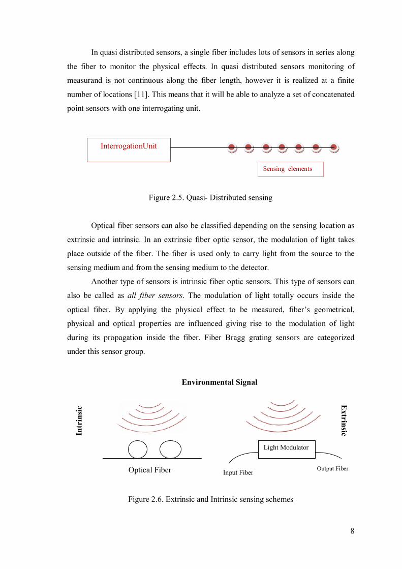
In quasi distributed sensors, a single fiber includes lots of sensors in series along
the fiber to monitor the physical effects. In quasi distributed sensors monitoring of
measurand is not continuous along the fiber length, however it is realized at a finite
number of locations [11]. This means that it will be able to analyze a set of concatenated
point sensors with one interrogating unit.
Figure 2.5. Quasi- Distributed sensing
Optical fiber sensors can also be classified depending on the sensing location as
extrinsic and intrinsic. In an extrinsic fiber optic sensor, the modulation of light takes
place outside of the fiber. The fiber is used only to carry light from the source to the
sensing medium and from the sensing medium to the detector.
Another type of sensors is intrinsic fiber optic sensors. This type of sensors can
also be called as all fiber sensors. The modulation of light totally occurs inside the
optical fiber. By applying the physical effect to be measured, fiber’s geometrical,
physical and optical properties are influenced giving rise to the modulation of light
during its propagation inside the fiber. Fiber Bragg grating sensors are categorized
under this sensor group.
Figure 2.6. Extrinsic and Intrinsic sensing schemes
Int
rins
ic
Extrinsic
Sensing elements
InterrogationUnit
Environmental Signal
Optical Fiber
Light Modulator
Input Fiber Output Fiber
9
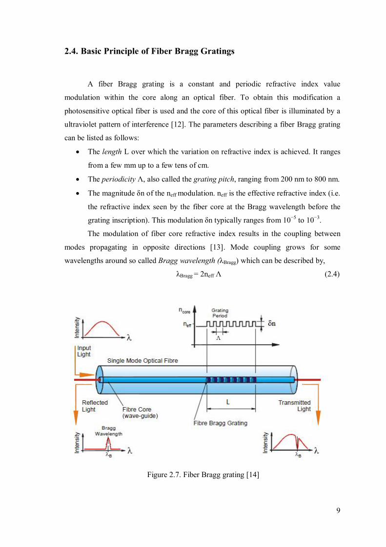
2.4. Basic Principle of Fiber Bragg Gratings
A fiber Bragg grating is a constant and periodic refractive index value
modulation within the core along an optical fiber. To obtain this modification a
photosensitive optical fiber is used and the core of this optical fiber is illuminated by a
ultraviolet pattern of interference [12]. The parameters describing a fiber Bragg grating
can be listed as follows:
The length L over which the variation on refractive index is achieved. It ranges
from a few mm up to a few tens of cm.
The periodicity Λ, also called the grating pitch, ranging from 200 nm to 800 nm.
The magnitude δn of the neff modulation. neff is the effective refractive index (i.e.
the refractive index seen by the fiber core at the Bragg wavelength before the
grating inscription). This modulation δn typically ranges from 10−5 to 10−3.
The modulation of fiber core refractive index results in the coupling between
modes propagating in opposite directions [13]. Mode coupling grows for some
wavelengths around so called Bragg wavelength (λBragg) which can be described by,
λBragg = 2neff Λ (2.4)
Figure 2.7. Fiber Bragg grating [14]

10
Physically the refractive index variation of the fiber Bragg grating give rise to a
weak Fresnel reflection with each period of the grating (Λ). The weak contributions are
added in phase and created a strong reflection for the Bragg wavelength. Therefore, a
fiber Bragg grating can be defined as a selective mirror around the Bragg wavelength as
schematically represented in Figure 2.7.
2.4.1. Model of the Uniform Bragg Grating
In uniform fiber Bragg gratings phase fronts is perpendicular along the fiber
longitudinal axis and plane of the grating has constant periodic refractive index
modulation. This kind of grating works as narrow-band reflective optical filter that
reflects a portion of the spectrum around the wavelength which satisfies Bragg
condition.
If the Bragg condition is not satisfied, light reflecting from the consecutive
planes will be out of phase and finally be canceled out. When the Bragg condition is
satisfied, contribution of light reflected from the each grating plane overlaps
constructively to the backward creating a reflected peak at the central wavelength which
is determined by the grating parameters.
Therefore, around the Bragg wavelength, FBG couples the light from the
forward propagating guided modes to backward propagating guided modes.
Figure 2.8. Wave vectors of uniform Bragg grating for Bragg condition
Bragg grating condition satisfies the conservation of energy and momentum. To
satisfy energy conservation, frequencies of both reflected and incident radiation need to
be equal [12].
h ωf = h ωi (2.5)
푘⃗ 푘⃗
퐾⃗

11
where h is the Planck constant (6.626 10−34 J.s) and ωi and ωf are the frequencies of the
incident radiation and the reflected radiation, respectively.
To satisfy momentum conservation, wavevector of incident wave k⃗ and grating
K⃗should be equal to the wavevector of scattered radiationk⃗. Here, grating wavevector
has a magnitude of Λ
and perpendicular to the grating planes (see Fig. 2.8).
푘⃗ + 퐾⃗ = 푘⃗ (2.6)
The diffracted wavevector is equal in magnitude, but opposite in direction, to the
incident wavevector. The conservation of momentum simplifies to the first order Bragg
equation and can be expressed as,
λBragg = 2 neff Λ (2.7)
where λBragg is the Bragg wavelength, neff effective refractive index of the fiber core at
the center wavelength, Λ grating periodicity.
2.4.2. Implementation of Transfer Matrix Method
To determine reflection and transmission spectra of an FBG in the presence of
mode coupling, coupled mode theory is used. This theory provides us an accurate
analytical solution for uniform fiber Bragg gratings.
In the framework of this thesis, the analytical solutions provided by the coupled
mode theory have been used as a starting point without demonstrating the whole steps
of the theory (these steps are given in Appendix A, Coupled Mode Theory).
The analytical results of the coupled-mode theory can be implemented in an
efficient way to model the reflection and transmission spectra of the grating in a
distributed manner all along the grating. Transfer matrix method is a simple and
precise technique which is easy to integrate into coupled mode equations [1].
In this method, grating is divided into N cascaded sections and each section is
affecting succeeding section. For instance, (N-1) th section’s matrix outputs are used as
the Nth section matrix inputs [13].

12
In this approach, the FBG can be considered as a 4-port device as shown in
Figure 2.9,
Figure 2.9. Input and output fields of Bragg grating
The forward-propagating fields R(0) and R(z), backward-propagating waves
S(0) and S(z), and the section length, ∆z = are represented in Figure 2.9. Transfer
matrix of the grating (T) comprises both the amplitude and phase information.
By the help of transfer matrix, input and output fields are connected to each
other as:
R(0)S(0) = [T] R
(z)S(z) (2.8)
In the case of reflection grating the reflected amplitude at input field of grating
R(0)is normalized to unity and output field amplitude S(z) is zero (i.e. backward-going
field does not exist further than the grating length as there is no perturbation away from
the end of the grating). Equation 2.8 is revised in the light of boundary conditions and
the relation is written as:
1S(0) = T T
T T R(z)0
(2.9)
R(z) = (2.10)
S(0) = (2.11)
R(0)
S(0)
R(z)
S(z)
Δz
Λ1
Δn1
Δz
Λ2
Δn2
Δz
ΛN-1
ΔnN-1
Δz
Λ3
Δn3
Δz
ΛN
ΔnN
0 Δz z z-Δz
T1 T2 T3 TN-1 TN

13
The entire grating after the Nth section can be defined as:
1S(0) = [T ]…..[T ][T ][T ] R(z)
0 (2.12)
The transfer matrix for the whole Bragg grating is the multiplication of all
individual section transfer matrices.
[T] = ∏ T (2.13)
Solving the couple mode theory equations given in Appendix A, elements of transfer
matrix are determined as,
T = cosh(αz) − ( ) (2.14)
T =− κ ( ) (2.15)
T = κ ( ) (2.16)
T = cosh(αz) + ( ) (2.17)
The parameters in equations from 2.14 to 2.17 are defined by the following
relationships,
Self-coupling coefficient σ = δ + σ (2.18)
AC coupling coefficient κ = πλ
υδn (2.19)
Tuning rate δ = β − πΛ= 2πn (
λ−
λ ) (2.20)
DC coupling coefficient σ = πλ
δn (2.21)
α = κ − σ (2.22)

14
The amplitude (r) and power (R) reflection coefficients of Bragg grating are
defined as
r = ( )( )
= (2.23)
r = κ (α )σ (α ) α (α )
(2.24)
(R = |r|2) R = ( )( )
(2.25)
The amplitude (t) and power (T) transmission coefficients of Bragg grating are
defined as
t = (1 − r) = ( )( )
= (2.26)
t =σ (α ) α (α )
(2.27)
(T = |t|2) T =( )
(2.28)
2.4.3. Amplitude Spectral Response of Uniform FBG: Some Examples
In this paragraph, the interesting features of fiber Bragg gratings is presented.
The numerical simulations for the evolution of power reflection coefficient R depending
on fiber length, average refractive index modulation and periodic refractive index
modulation have been plotted versus normalized wavelength defined by λ /λmax.
λmax = (1+ ) λBragg (2.29)
λmax = 2 (neff + 훿푛) Λ (2.30)
where λmax is wavelength at where the maximum reflectivity occurs. In figure 2.10 the
relation between the reflected and transmitted spectra are observed as,
R(λ) + T(λ) = 1 (2.31)

15
Figure 2.10. Reflection and transmission spectra of a uniform fiber Bragg grating.
Parameters used for the simulation: as ν=0.5; δn=1x10⁻⁴; Λ=540 nm; L=1cm
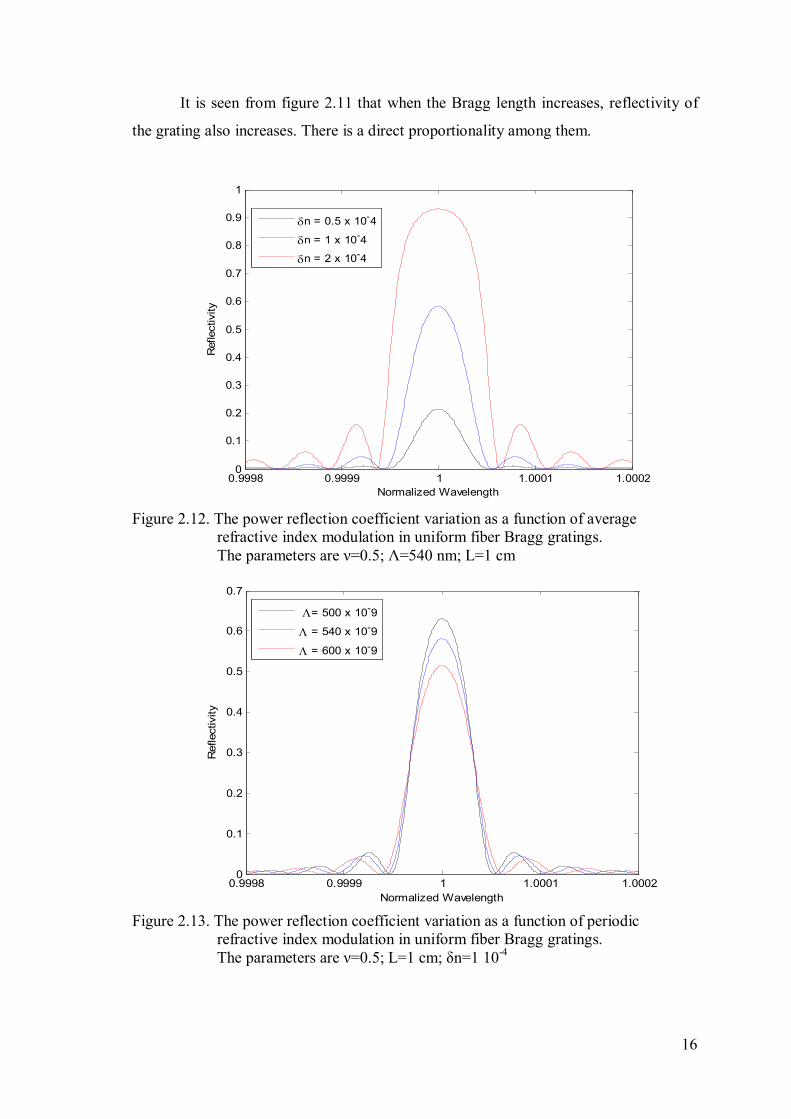
In figures 2.11, 2.12 and 2.13, the effect of grating length (L), average refractive
index modulation (δn) and periodic refractive index modulation (Λ) on the reflection
spectrum are presented, respectively.
Figure 2.11. The power reflection coefficient variation as a function of grating length in
uniform fiber Bragg gratings. The parameters are ν=0.5; Λ=540 nm; δn= 1x10⁻⁴
1565 1565.5 1566 1566.5 1567 1567.50
0.1
0.2
0.3
0.4
0.5
0.6
0.7
0.8
0.9
1
Wavelength (nm)
Ref
lect
ivity
& T
rans
mitt
ivity
RT
0.9998 0.9999 1 1.0001 1.00020
0.1
0.2
0.3
0.4
0.5
0.6
0.7
0.8
0.9
1
Normalized Wavelength
Ref
lect
ivity
L = 0.5 cmL = 1 cmL = 2 cm
16
It is seen from figure 2.11 that when the Bragg length increases, reflectivity of
the grating also increases. There is a direct proportionality among them.
Figure 2.12. The power reflection coefficient variation as a function of average
refractive index modulation in uniform fiber Bragg gratings. The parameters are ν=0.5; Λ=540 nm; L=1 cm
Figure 2.13. The power reflection coefficient variation as a function of periodic refractive index modulation in uniform fiber Bragg gratings. The parameters are ν=0.5; L=1 cm; δn=1 10-4
0.9998 0.9999 1 1.0001 1.00020
0.1
0.2
0.3
0.4
0.5
0.6
0.7
0.8
0.9
1
Normalized Wavelength
Ref
lect
ivity
n = 0.5 x 10⁻⁴
n = 1 x 10⁻⁴
n = 2 x 10⁻⁴
0.9998 0.9999 1 1.0001 1.00020
0.1
0.2
0.3
0.4
0.5
0.6
0.7
Normalized Wavelength
Ref
lect
ivity
= 500 x 10-9
= 540 x 10-9
= 600 x 10-9

17
In Figure 2.12 the effect of the core refractive index modulation on the reflection
spectrum is observed. It is obvious from the figure that reflectivity increases when the
refractive index modulation increases.
Figure 2.11 and 2.12 also show that the spectral bandwidth between first zeros
increases when δn increases and/or when L decreases.
The evolution of the power reflectivity (R) with respect to periodic refractive
index variation (Λ) is shown in Figure 2.13. Contrary to L and δn variation, an increase
on the periodic refractive index value decreases the reflectivity of FBG.
2.4.4. Advantages of Fiber Bragg Gratings
Fiber optic sensors (FOS) have been gaining a remarkable position in
marketplace thanks to their advantages compared to conventional sensors that are listed
as follows:
The information of the measurand is wavelength-encoded. This property makes
the sensor self-referencing and independent from the fluctuations of light power
levels that might rise on the system. Therefore the system is unaffected from the
source power fluctuations, detector sensitivity changes, connector losses, or by
the presence of other FBGs at different wavelengths. This property is the main
advantage of the FBG-based sensors.
Multiplexing is one of the most important advantages of optical fibers. Sensing
points can be placed in series on the same optical fiber. The multiplexing ability
provide us monitoring different types of sensors along the same fiber like strain
sensors and thermal sensors.
Linear response to the physical parameter to be measured over large ranges.
Optical fibers have low attenuation, so it is easy to monitor sensing locations
from a remote interrogation station at large distance (the interrogation unit can
be placed tens of kilometers away from the sensing points).
Easy to install: just one optical fiber is required to bond to the structure and
connected to the interrogator.
Because of their small size and geometric versatility FBG sensors can easily
be embedded into various structures to provide damage or strain detection and
offer the best option in hard-to-reach and space-limited environments.

18
Optical fibers are safe, passive because they don’t need to use electricity to
work. That is why there will be no risk of fires or explosions. This is an
important issue for the nuclear or chemical applications.
They have long durability, as they are composed of rugged passive
components.
In addition to above advantages, FBGs are also immune to electromagnetic interference
and low in price [15], [16].
2.4.5. Applications of Fiber Bragg Gratings
Application areas of fiber Bragg gratings are several. Some of them are listed as,
Aerospace: Structural health monitoring, maintenance of safety and integrity in
aerospace structural system [17].
Medical: Used as pressure sensor to measure muscular strength of hands or
weight profile of patients [18].
Renewable wind energy: Monitoring strain distribution along the wind turbine
wing [19].
Civil structures: Implementation of fiber Bragg gratings array in to the bridges,
tunnels, buildings, and dams to monitor structural health.
Automotive: Frame stress detection to increase safety.
Transportation and Rail: Monitoring deformation on the rail, imbalance or
strain on the wheels in high-speed railways or trains carrying overloads [20].
Marine: Monitoring fast military vessels, racing yachts, and sub-sea vessels
[21].
Oil and Gas: Humidity and hydrogen detection, monitoring oil, gas, water and
waste pipelines.
Power: Vibration and temperature monitoring on the nuclear power plants [22].

19
CHAPTER 3
FIBER BRAGG GRATING INTERROGATION
TECHNIQUES
3.1. Introduction
This chapter describes detection schemes for fiber Bragg grating sensors. All
interrogation types are differing in system performance as well as in system complexity,
robustness, and costs.
As already presented in the previous chapter, fiber Bragg gratings are intrinsic
optical sensors where the wavelength of the reflected (or transmitted) spectrum is
shifted as a function of external parameter to be measured.
To interrogate the FBGs, a straightforward approach might be the wavelength
interrogation of the reflected or transmitted spectral components. General principle of
the wavelength measurement is to convert wavelength shift to some measurable
parameters such as amplitude, phase or frequency.
Since this thesis focuses on one of the optical reflectometry technique which is
optical frequency domain reflectometry, the other interrogation techniques are
summarized briefly.
3.2. Wavelength Detection Techniques
In all wavelength detection techniques, the set-up contains broadband light
source to illuminate the fiber Bragg grating. Light coming from this source is coupled to
the optical fiber and reflected light from fiber Bragg grating sensor is analyzed by a
wavelength detection scheme.

20
Linearly wavelength dependent optical filter; In this type of detection scheme,
Bragg wavelength shift is monitored depending on power variation. Although this
method has a simple scheme, it is not easy to apply multiplexed FBGs to this scheme.
Moreover, the measurements are affected by the power fluctuations. The set-up of
measurement contains a filter, a broadband light source and fiber Bragg grating. The
ratio of the reflected signal intensity between the reference arm and the filter’s arm is
changed linearly depending on the Bragg wavelength shift [23].
Linearly wavelength dependent optical coupler; In this method, main
component of the set-up is wavelength division multiplexing (WDM) coupler. WDM
coupler has a linear and opposite response in the coupling ratios between input and
output ports. This coupler receives the reflected light from Bragg grating to detect the
wavelength shift. This shift is achieved by computing (linear change) the ratio between
sum and difference of output arms of the couplers [24].
These two methods explained above use passive components at the detection
schemes.
Figure 3.1. Scheme of Wavelength Division Coupler interrogation system
푃 − 푃푃 + 푃
P1
P2
P1/P
P2/P
λ
Wavelength encoded
optical signal
WDM fiber Coupler

21
Detection with a scanning optical filter; One of the most attractive
interrogations to measure the wavelength shift of a Bragg grating is based on the use of
a tunable filter for tracking the spectrum reflected from the grating.
The filter center is tuned until the multiplication of fiber Bragg grating and
scanning filter spectra match, at the match condition the system output takes its
maximum. Different applications for this method are available and some of them can be
found in [25], [26], [27].
Fiber Optic Interferometer; In this technique, interferometer converts the
wavelength shifts at back reflected light coming from grating to the phase variation.
When comparing with the other detection techniques fiber optic interferometry has
more wavelength sensitivity [28]. To convert the wavelength shift to the phase
variation, reflected spectrum of Bragg grating topazes through an interferometer which
has a wavelength dependent transfer function with the form (1+cosø) (the ø phase term
depends on the input wavelength).
3.3. Optical Reflectometry Techniques
In this paragraph, Optical Time Domain Reflectometry (OTDR) measurement
technique is presented then study about the Optical Frequency Domain Reflectometry
(OFDR) technique are detailed.
Optical reflectometry can be classified into two categories as direct-detection
and coherent-detection. In direct detection, only the optical reflected signal is incident
on the photodetector but in coherent detection reflected signal and a reference optical
signal are incident on the photodetector [29].

22
3.3.1. Optical Time Domain Reflectometry (OTDR)
Optical Time Domain Reflectometry’s basic principle is to detect and analyze the
scattered light coming from small imperfections, inhomogeneities and impurities in the
optical fiber. Conventional OTDRs use Rayleigh backscattering to determine the
location of fiber breaks, the fiber attenuation coefficient, splice loss, and various other
link characteristics. By using OTDR some parameters can be measured and provided;
Distance to splice loss, connector loss, bend loss and their quantities.
Reflectivity of mechanical splices, connectors
Active monitoring on live fiber optic system
Fiber slope and fiber attenuation
Figure 3.2. Principle diagram of an OTDR
A basic OTDR diagram is shown in Figure 3.2. Light coming from a laser is
connected to a coupler. When the pulse propagates along the fiber, some of its power is
lost because of Rayleigh scattering, absorption and radiation loss [30].
The most significant loss in OTDR measurements is Rayleigh scattering. The
80-90% of the total loss of light is produced by Rayleigh scattering. Microscopic
inhomogeneities at the refractive index of the fiber create this scattering.
The probe signal can also be attenuated due to splices, bends or connectors at
discrete locations in the fiber as shown in Figure 3.3.
Laser
Receiver
Coupler
Connector
Terminated
Test Fiber

23
1 Reflection from Front Connector
2 Fiber Attenuation
3 Non-Reflective Loss (Fusion Splice or Bending)
4 Reflective Loss (Mechanical Splice or Connector)
5 Fiber End Reflection
6 Noise Level
Figure 3.3. Events on a typical OTDR trace
When the optical pulse is sent to the fiber and it meets with a discontinuity in the
refraction index, some of the signal energy is reflected back and coupler directs it to the
optical receiver. An OTDR software displays the losses on a generated graph and
provides the loss value in dB as a function of distance.
The received power is measured as a function of time. Then a conversion is
needed to obtain measurements in length (in km). Because of light travels forward and
backward directions before reaching the receiver, it propagates twice the distance.
The OTDR software multiplies the time value by the group velocity of the light
in the fiber, in order to convert time into a one-way distance. That is why optical power
is computed by using 5log10 formula not with 10log10 formula [31].
Some key parameters are considered when investigating the performances of an
OTDR.
ATT
ENU
ATI
ON
(dB
) 1
2 3
4 5
6
DISTANCE (km)

24
The dynamic range of an OTDR is defined as the strength of the initial
backscattering level to the noise level. It shows the maximum loss the equipment is able
to measure. To increase the OTDR’s dynamic range, backscatter level should be
increased and noise should be decreased. (see Fig. 3.4)
Figure 3.4. Dynamic Range
The spatial resolution parameter gives the information about capability of
OTDR to resolve two close events. The spatial resolution length depends on optical
pulse width (half of the pulse width).
In an OTDR measurement, there is a trade-off between spatial resolution and
dynamic range. When shorter pulses (narrow pulse width) are used to provide good
spatial resolution, the signal to noise ratio is worse because of the smaller backscattered
power (decreasing in the pulse energy is decreasing the signal level), so the attainable
dynamic range is smaller. In contrast, when the pulse width is broadened dynamic range
becomes larger but spatial resolution becomes worse.
After having received a strong reflection, the OTDR receiver is blinded
(saturation) during a certain time interval. There is a distance after the reflection peak
where no proper measurement can be performed. This region is denoted by the term
dead zone.
To interrogate FBGs by OTDR, several techniques are proposed where the
OTDR provides information about position, magnitude and phase of the reflective
events (FBGs in this case).

25
To extract the wavelength shift information some signal processing is required
as shown schematically in Figure 3.5.
Figure 3.5. Optical reflectometry techniques for FBG interrogation
Conventional OTDR is one of the applications for interrogation of FBGs. As
shown in Figure 3.6, sensor pairs are interrogated by OTDR. The physical parameters
are not applied on the reference grating. The reference grating is used to compensate
power fluctuations on the source. The whole range of the wavelength is used by the
OTDR source and back reflected signal from the sensing grating is measured by OTDR
receiver. The Bragg wavelength shift can be obtained by the linear change in the
measured power according to the linear edge of the source spectrum [32].
The wavelength of the sensing grating is located at the increasing or decreasing
edge of the source spectrum to obtain maximum power variation as a function of
wavelength shift.
Figure 3.6. Conventional OTDR scheme
Reflectometer
….
Signal
Processing
Wavelength
shift
pow
er
distance
FBG FBG FBG
OTDR
FBG FBG
Reference Sensing FBG FBG
Reference Sensing
#1 FBG pair 2# FBG pair

26
OTDR with an adjustable Fabry-Perot filter, This method is based on the
association of a commercial OTDR with a band pass filter. The schematic of the
proposed system is shown in figure 3.7. A concatenation of several arrays of fiber
Bragg gratings (FBG1 . . . FBGn) is interrogated.
The FBGs in each array have got approximately the same nominal Bragg
wavelengths, λ1 . . . λn. The passband of the Fabry-Perot filter (1.3 nm) is slightly
narrower than the FWHM of the Bragg gratings (1.5 nm). When the reflection spectrum
of a given FBG coincides with the passband of the FP filter, a detectable signal will be
generated at the OTDR receiver. By using low reflective gratings, several FBGs at the
same nominal wavelength but at different positions (hence with different delay times)
can be addressed simultaneously for a given center wavelength of the filter [33].
Figure 3.7. Scheme of OTDR with a spectral filtering
Wavelength Tunable OTDR: as shown in Figure 3.8 a wavelength conversion
system is combined with a conventional OTDR. The optical pulses emitted from a
conventional OTDR are first converted to electrical pulses and then modulate the
Tunable Laser Source (TLS) at the desired wavelength [34].
Optical pulses obtained at the desired wavelength are sent to the FBGs. The
reflected light from FBGs is directed to the OTDR. Tunable laser source scans the
proper set of wavelength and using a set of OTDR traces obtained these wavelenghts,
the reflection spectra of all FBGs are reconstructed.
OTDR
( FBG 1 … FBG n)1
λ1 ... λn
(FBG 1 … FBG n)2
λ1 ... λn PC Adjustable
spectral band pass

27
*
Figure 3.8. Wavelength tunable OTDR interrogation scheme
3.3.2. Coherent- Optical Frequency Domain Reflectometry (OFDR)
When the optical system under consideration is several tens of meters in length,
OFDR can be used because of its millimeter resolution, high sensitivity and large
dynamics. OFDR overcome the limitations of OTDR on spatial resolution, dynamic
range and measurement speed for the immediate and definite detection of any structural
damage.
To interrogate fiber Bragg grating spectrum, coherent-optical frequency domain
reflectometry is the best suited method providing high spatial resolution between two
measured point over multiple tens of meters of optical length [35].
Optical frequency domain reflectometry (OFDR) technique works with similar
principle as optical time domain reflectometry (OTDR) technique and provides
information about reflection and transmission spectrum on the measurand. OTDR is
based on direct detection scheme but OFDR is operating in coherent detection mode.
OTDR O/E conversion +
pulse generation
TLS
FBG FBG
Wavelength Conversion System (WCS)
C1
C2

28
3.3.2.1. Principle of OFDR
In its basic configuration, the optical carrier frequency of a tunable laser source
(TLS) is swept linearly in time without mode hops. Then, the frequency modulated
continuous-wave signal (probe signal) is split into two paths (see figure 3.9), namely the
test arm and the reference arm.
The test signal which is reflected back from the reflection sites in the test arm
coherently interfere at the coupler with the reference signal returning from the reference
reflector. This interference signal contains the beat frequencies which appear as peaks at
the network analyzer display after the Fourier transform of the time-sampled
photocurrent [36].
Using a linear optical frequency sweep, the measured beat frequencies can be
mapped into a distance scale (the proportionality factor between beat frequency and the
corresponding distance is determined by the rate of change of the optical frequency),
while the squared magnitude of the signal at each beat frequency reveals the reflectivity
of each reflection site. This method is often called as coherent FMCW (Frequency-
Modulated Continuous Wave) [37].
Figure 3.9. Basic configuration of distributed C-OFDR
Linearly-chirped
source
Receiver
FFT spectrum
analyzer
Optical Frequency
t
coupler
Local Oscillator
(Reference arm)
Device Under Test
(Test Arm)
L

29
In this thesis the formulation is described by the wavenumber of light and results
of the analysis are presented in terms of wavelength of the light. The relation between
wavenumber k and wavelength can be expressed as,
푘 = (3.1)
The intensity measured at the detector varies as a cosine function of the
wavenumber k and can be expressed as in equation 3.2 (derived in the Appendix B
[38]),
퐷 = cos 2푛 푘퐿 (3.2)
where neff is the effective refractive index of optical fiber core.
This equation shows that light reflected from device under test and light
reflected from the reference reflector have an optical path difference of 2neffL.
Due to the linear modulation of the optical frequency, each reflection on side on
the optical fiber corresponds to a beat frequency. These beat frequencies can be
observed by taking the Fourier transform of the interference signal and then can be
converted into distance [39].
As the laser is tuned light intensity observed by dedector varies depending on
wavenumber change Δk and can be expressed as [40],
Δk = (3.3)
The schematic of the Fourier and Inverse Fourier Transform application can be
shown in Figure 3.9 and 3.10.
The Fourier transform separates the interference signal waveform into sinusoids
of different frequencies.

30
Figure 3.10. Spectral mapping between wavenumber and length [41]
By using a bandpass filter around a proper position of a reflection and by
applying an inverse Fast Fourier transform to the filtered signal, the spectrum of each
reflection can be obtained independently from the others.
Figure 3.11. Schematic of demodulation process [41]
In summary, to obtain the reflection spectra of a reflection side (this could be a
FBG or a discrete reflection) in the test arm of the OFDR, a band-pass filter (centered at
a particular beat frequency, hence position) is used to extract the portion having the
information related to this particular reflection.
1547.7 1547.8 1547.9 1548 1548.1 1548.2 1548.3 1548.4 1548.5 1548.6 1548.70
0.005
0.01
0.015
0.02
0.025
n Lπ cos(2푛 퐿푘)

31
This is followed by an inverse Fast Fourier transform to recover the complex
FBG spectrum and the obtained spectrum is called as demodulated reflection
(transmission) spectrum. Steps to obtain demodulated spectrum can be shown in figure
3.12 where identical uniform FBGs are used as reflection points [37].
Figure 3.12. Schematic of signal processing
The flowchart belong to above explained signal process is represented in Figure 3.13 as,
Figure 3.13. Flowchart of signal processing
OFDR
IFFT
OFDR trace
λB λB λB
Demodulated
Transmission
spectra
FBG1 FBG2 FBGN
frequency
Interference
Signal
Analysis Signal
C-OFDR
spectrum
Demodulated
Reflection Spectrum
Band-pass filter
around beat
frequency
Physical Effect
Δλ

32
Matlab Simulation Example
As an example to above discussion, we simulated the OFDR trace when there is
one FBG in the test arm at the position: 1.38 m. In these simulations the reflectivity of
Bragg grating is derived by using equations 2.28, the interferometer signal is examined
and the location information is provided by taking Fourier transform of the signal.
Inverse Fourier transform of the signal allows demodulating the reflection coefficient of
fiber Bragg grating. Finally theoretical reflection coefficient is compared to the
demodulation result in Figure 3.15. The simulation parameters are as follows:
Table 3.1. Parameters used for Matlab simulation
Visibility 1
z (location of FBG) 1.38 m
neff (effective refractive index) 1.45
L (Fiber Bragg grating length) 200 mm
δneff (Average index change) 1.6 x 10⁻⁵
λBragg (Bragg wavelength) 1583.7 nm
Λ (periodic refractive index change). 547.59 nm
NoP (Number of point used in Fourier
transform)
40000

33
Figure 3.14. Reflectivity of FBG found by mathematical derivation (Eq.2.25)
Figure 3.15. Comparison of demodulated signal with the mathematically obtained
1583 1583.2 1583.4 1583.6 1583.8 1584 1584.2 1584.4
0.01
0.02
0.03
0.04
0.05
0.06
0.07
0.08
0.09
0.1
Wavelength(nm)
Ref
lect
ivity
1583.2 1583.4 1583.6 1583.8 1584 1584.2 1584.4
0.1
0.2
0.3
0.4
0.5
0.6
0.7
0.8
0.9
1
Wavelength(nm)
Nor
mal
ized
Ref
lect
ion
Am
plitu
de
Reflection Spectra (OFDR Signal)Reflection Spectra (Original Signal)

34
Figure 3.16. Simulated OFDR trace
3.3.2.2. OFDR Interrogation of Fiber Bragg Grating by using Transfer
Matrix Method
In previous examples, the results are obtained by using the analytical approach
derived in the Appendix B. This approach does not permit us to realize a distributed
analysis along the length of the FBG. In this part, we implement the Transfer matrix
method to model the FBG interrogated by the OFDR. In the model, there is a single
FBG on the test arm of the OFDR as shown in Figure 3.17.
In order to simulate detector signal (D), FBG and mirror are modeled on the C-
OFDR system. The model is determined based on transfer matrix method as mentioned
in section 2.4.4. Fiber Bragg grating is divided into N uniform section and each section
length is Δz long [42].
1.34 1.35 1.36 1.37 1.38 1.39 1.4 1.41 1.42 1.43
0
1
2
3
4
5
6
7
8x 10⁻³
position(m)
Pow
er(a
rb. u
nit)

35
Figure 3.17. Model of FBG and mirror on C-OFDR system (TLS: Tunable Laser
Source, PD: Photodetector, C: Coupler)
The elements of the grating matrices FB1…N is formed by equations and is
expressed as,
T = cosh(αL) − ( ) (3.4)
T =− κ ( ) (3.5)
T = κ ( ) (3.6)
T = cosh(αL) + ( ) (3.7)
TLS
PD
C Fiber Bragg Grating
D
L
PBragg
0 z0 z1
Pmirror
Mirror
z2
z1 z2
FB1
FB2
FB3
…
…
…
…
…
…
FBN
Δz Δz Δz Δz
R(z2)
S(z2)
R(z0)
S(z0)
36
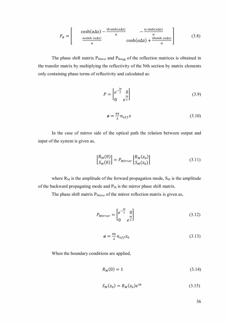
퐹 =cosh(αΔz) − ( ) − κ ( )
κ ( ) cosh(αΔz) + ( ) (3.8)
The phase shift matrix PMirror and PBragg of the reflection matrices is obtained in
the transfer matrix by multiplying the reflectivity of the Nth section by matrix elements
only containing phase terms of reflectivity and calculated as:
푃 = 푒ø0
0푒ø (3.9)
ø = 푛 푧 (3.10)
In the case of mirror side of the optical path the relation between output and
input of the system is given as,
푅 (0)푆 (0) = 푃 푅 (푧 )
푆 (푧 ) (3.11)
where RM is the amplitude of the forward propagation mode, SM is the amplitude
of the backward propagating mode and PM is the mirror phase shift matrix.
The phase shift matrix PMirror of the mirror reflection matrix is given as,
푃 = 푒ø0
0푒ø (3.12)
ø = 푛 푧 (3.13)
When the boundary conditions are applied,
푅 (0) = 1 (3.14)
푆 (푧 ) = 푅 (푧 )푒 (3.15)

37
1푆 (0) = 푃 푃
푃 푃푅 (푧 )
푅 (푧 )푒 (3.16)
The mirror reflection coefficient is given as,
푅퐿 = 푆 (0) = (3.17)
푅퐿 = 푒 ( ) (3.18)
For the optical path contains fiber Bragg grating, the transfer matrix (T) for the
whole optical path is considered as the multiplication of the transfer matrices of all the
individual FBG sections and express as,
T=PBraggFB1FB2……FBN (3.19)
where PBragg is Bragg phase shift matrix and given as,
푃 = 푒ø0
0푒ø (3.20)
ø = 푛 푧 (3.21)
The relation between input and output of the Bragg system is defined by the
equation 3.22,
푅 (0)푆 (0) = 푇 푇
푇 푇푅 (푧 )푆 (푧 ) (3.22)
where RB is the amplitude of the forward propagating mode and SB is the amplitude of
the backward propagating mode.

38
The boundary conditions for the Bragg system is defined as,
푅 (0) = 1 (3.23)
푆 (푧 ) = 0 (3.24)
When the boundary condition is applied on equation 3.22, the reflection
coefficient for Bragg grating cab be defined as,
푅퐿 = 푆 (0) = (3.25)
Finally the output signal observed by detector (D) is calculated by using two-
beam interference method and given by [7],
퐷 = 푅퐿 + 푅퐿 푅퐿 + 푅퐿∗ (3.26)
퐷 = 푅퐿 + 푅퐿 (3.27)
Matlab Implementation
In this part, mathematical model is verified for the above scheme (Figure 3.17)
with the Matlab simulations. Figures 3.18, 3.19, 3.20, 3.21 and 3.22 are obtained by
using equations from 3.4 to 3.27. The parameters used in simulations are as follows,
Table 3.2. Parameters used for the Matlab implementation of OFDR
Visibility 0.3944
z0 (absolute location of the mirror) 1 m
z1 (location of FBG) 4.96 m
neff (effective refractive index of fiber core) 1.45
L (Fiber Bragg grating length) 200 mm
δneff (Average index change) 3.10 x 10⁻⁶
λBragg (Bragg wavelength) 1548.163 nm
N (number of FBG section) 100

39
In figure 3.18, the reflection spectrum of a uniform fiber Bragg grating is
obtained by using Transfer Matrix Method. This results that Bragg grating reflects %20
of the incident signal. Figure 3.19 shows the composite detector signal, D which is
normalized by its maximum value at the Bragg wavelength (1548.163 nm)
Figure 3.18. Evolution of Fiber Bragg Grating reflection spectrum by transfer matrix method
Figure 3.19. Output signal calculated by photodetector
1548.14 1548.15 1548.16 1548.17 1548.18 1548.19
0.02
0.04
0.06
0.08
0.1
0.12
0.14
0.16
0.18
0.2
0.22
Wavelength(nm)
Ref
lect
ivity
1547.7 1547.8 1547.9 1548 1548.1 1548.2 1548.3 1548.4 1548.5 1548.6 1548.70.1
0.2
0.3
0.4
0.5
0.6
0.7
0.8
0.9
1
Wavelength(nm)
Out
put S
igna
l Pow
er(a
.u.)

40
In Figure 3.20, the Fourier transform of interference signal is taken to obtain the
OFDR trace showing the power reflected from the FBG as a function of position. The
reason of the power decrease along the grating length is the loss of the light when it
propagates though the grating.
Figure 3.20. Simulated beat spectrum of the interferometer
In Figure 3.21 Inverse Fourier transform is applied on the selected position
(between 4.96 m- 5.16 m) as explained before to “demodulate” the reflection spectrum
of the FBG. This demodulated reflection spectrum is then compared with the original
reflection spectrum where a good agreement is observed between the two approaches.
This means that our demodulation process works well and our simulation results match
with the theoretical values.
4.85 4.9 4.95 5 5.05 5.1 5.15 5.2 5.25 5.30
0.002
0.004
0.006
0.008
0.01
0.012
Position(m)
Det
ecte
d S
igna
l(a.u
.)

41
Figure 3.21. Comparison of demodulated signal with calculated reflectivity
Figure 3.22 represents the spectrogram of the output signal D. The spectrogram
is obtained by applying Short Time Fourier Transform of the signal and provides the
spectrum information in 3 dimensions, namely, wavelength, position and intensity.
To perform STFT, a proper window (Hanning window is used in simulations) is
applied for a definite wavelength, the information about the signal around focused
wavelength is obtained.
Then by using Fast Fourier Transform the extracted signal analyzed and each
frequency components power in the output signal is achieved.
Sliding the window to all wavelengths and performing Fourier transform
provided us three dimensional information that includes wavelength information at the
x-axis, position information at the y-axis and colored part shows the power of the
signal.
1548.13 1548.14 1548.15 1548.16 1548.17 1548.18 1548.19 1548.2
0.1
0.2
0.3
0.4
0.5
0.6
0.7
0.8
0.9
1
Wavelength(nm)
Nor
mal
ized
Ref
lect
ion
Am
plitu
de
Reflection Spectra(OFDR Sİgnal)Reflection Spectra (Original Signal)

42
Figure 3.22 Spectrogram of interference signal
In figure 3.22 the red colored part of the spectrogram denotes the highest
intensity regions from red to dark blue region the intensity of light is increase. It is
logical because of the reflection is occurs at the Bragg wavelength 1548.16 for this
simulation and the intensity of light is expanded around this wavelength.
Wavelength(nm)
Pos
ition
(m)
1547.8 1547.9 1548 1548.1 1548.2 1548.3 1548.4 1548.5 1548.6
0
1
2
3
4
5
6
7
Wavelength(nm)
Pos
ition
(m)
1547.95 1548 1548.05 1548.1 1548.15 1548.2 1548.25 1548.3 1548.35
4.4
4.6
4.8
5
5.2
5.4
5.6
5.8

43
Under a physical effect applied on Bragg grating, the Bragg wavelength shifts
differently proportional to the applied effect. Figure 3.23 and 3.24 shows shift on the
reflection coefficient of the fiber Bragg grating and shift on the detector signal under
applied strain. In this simulation the Bragg wavelength shift is 0.2 nm at its center in
other words it shifts from 1548.16 nm to 1548.36 nm. So the output and reflection
spectrum is separated by 0.2 nm.
Figure 3.23. Reflection spectrum of uniform FBG for 0.2 nm shifts
Figure 3.24. Output signals for 0.2 nm shifts
1548.1 1548.15 1548.2 1548.25 1548.3 1548.35 1548.4
0.02
0.04
0.06
0.08
0.1
0.12
0.14
0.16
0.18
0.2
Wavelength(nm)
Ref
lect
ion
Am
plitu
de
No Strain AppliedApplied Strain
1548.1 1548.15 1548.2 1548.25 1548.3 1548.35 1548.4
0.4
0.5
0.6
0.7
0.8
0.9
1
Wavelength(nm)
Out
put S
igna
l(a.u
.)

44
Figure 3.25. Spectrogram of the 0.2 nm shifted interference signal
Wavelength(nm)
Pos
ition
(m)
1548 1548.1 1548.2 1548.3 1548.4 1548.5
0
1
2
3
4
5
6
7
Wavelength(nm)
Pos
ition
(m)
1548 1548.1 1548.2 1548.3 1548.4 1548.5
4.7
4.8
4.9
5
5.1
5.2
5.3
5.4
5.5

45
In figure 3.25 the reflection center wavelength shift is obtained in spectrogram.
Bragg wavelength. The spectrogram is obtained by appliying STFT on the detector
signal. The reflected light is sampled by 0.14 1/m (Δk) wave number spacing. This
results a 0.053 pm wavelength spacing (Δλ). Analysis is done by using 4000 points
Hanning window and FFT is applied to 214 points. Window is slided 20 points. The
window length is choosed as 4000 point due to influencing distance and wavelength
resolution. Here figures show that applied strain effects amount of wavelength shift on
the Bragg wavelength.

46
CHAPTER 4
POLARIZATION CONCEPTS
4.1. Introduction
Fiber Bragg gratings that studied in Chapter 2 is manufactured by exposing one
side of the optical fiber to an intense UV interference pattern. It is accepted that the
writing process of the fiber leads to small amount of birefringence. This quantity
combines with the intrinsic birefringence. The small birefringence values have
significant polarization dependent effects on Bragg gratings. In this chapter, the basic
phenomena of the polarization of light are studied. Then, the mathematical formalism to
define the state of the polarization is examined. Birefringence term and the effect of this
phenomenon to the uniform fiber Bragg gratings are also explained in detail. Finally,
the effect of grating parameters (physical length, refractive index modulation) and the
value of the birefringence on the Polarization Dependent Loss (PDL) are studied.
4.2. Polarization of Light
A polarized lightwave signal propagating in free space or in a waveguide like
optical fiber can be described by electrical and magnetic field vectors perpendicular to
each other in a transverse plane and perpendicular to the direction of propagation [43].
The state of polarization is presented by the pattern plotted by electrical field
vector as a function of time at a fixed point in a transverse plane [44].

47
Figure 4.1. Concept of polarization of light
To present the polarized light propagating along the z direction mathematically
(in terms of the x and y axis projections of electrical field vector), x and y components
of the electric field at z=0 given by,
퐸 = 휀 푒 ; 퐸 = 휀 푒 (4.1)
휀 = 퐸 푒 ; 휀 = 퐸 푒 (4.2)
퐸 (푧, 푡) = 퐸 cos(휔푡 + 훿 − 푘푧) (4.3)
퐸 (푧, 푡) = 퐸 cos(휔푡 + 훿 − 푘푧) (4.4)
where E0x and E0y are the maximum amplitudes, δx and δy are the corresponding phases.
The pattern drawn by electrical field is found by eliminating (ωt-kz) term from the
equations 4.3 and 4.4 so the relation is define as,
+ − 2 cos δ = sin 훿 (4.5)
where δ= δx- δy is the phase difference between x and y components.
Equation 4.5 is the polarization ellipse equation trace out in the transverse plane
by the tip of the electrical field vector in a fixed point of space and as a function of time
[45]. Fully polarized light wave’s state of polarization is elliptical by the equation it is
obvious that state of polarization depends three parameters E0x, E0y and δ. This ellipse is
presented in figure 4.2.
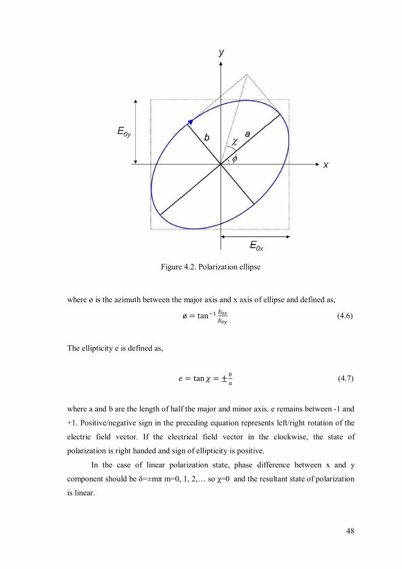
48
Figure 4.2. Polarization ellipse
where ø is the azimuth between the major axis and x axis of ellipse and defined as,
ø = tan (4.6)
The ellipticity e is defined as,
푒 = tan휒 = ± (4.7)
where a and b are the length of half the major and minor axis. e remains between -1 and
+1. Positive/negative sign in the preceding equation represents left/right rotation of the
electric field vector. If the electrical field vector in the clockwise, the state of
polarization is right handed and sign of ellipticity is positive.
In the case of linear polarization state, phase difference between x and y
component should be δ=±mπ m=0, 1, 2,… so χ=0 and the resultant state of polarization
is linear.

49
4.2.1. Jones Vector Formalism of Polarized Light
Polarization variation of an incident wave when it passes through an optical
component can be described by three formalisms:; Jones calculus, Mueller calculus, and
the Poincaré sphere.
Between 1941 and 1948 Clark Jones proposed a mathematical representation of
polarized light based on optical fields. This method represents a given SOP by only a
two dimensional vector of complex numbers known as Jones vector and uses simple 2 ×
2 matrices to calculate the effect of a polarizer or a birefringent medium for a given
state of polarization (SOP) [46].
Description of the electric field vector of an arbitrarily polarized light wave in
terms of two orthogonal and linearly polarized components can be written as,
퐸(푧, 푡) = 퐸 cos(휔푡 + 훿 − 푘푧) 풙 + 퐸 cos(휔푡 + 훿 − 푘푧)풚m (4.8)
The SOP is defined in terms of a 2 × 1 matrix as,
퐸(푧, 푡) =퐸퐸 =
퐸 cos(휔푡 + 훿 − 푘푧)퐸 cos(휔푡 + 훿 − 푘푧) (4.9)
퐸(푧, 푡) =퐸 e퐸 푒
= e퐸퐸 e (4.10)
When the common phase factor is omitted to simplify the representation of the
phases, equation 4.10 is written as,
퐸(푧, 푡) =퐸퐸 e (4.11)
To normalize the Jones vector given by Equation 4.11, the amplitudes E0x and
E0y are divided by 퐸 + 퐸 and obtained as,
퐸(푧, 푡) =퐸퐸 e (4.12)

50
A linearly polarized wave of amplitude E0x making an angle ø with the x axis
can be described as a superposition of the x- and y polarized components. Thus, the
corresponding normalized Jones vector is given by,
퐸(푧, 푡) = cosø푠푖푛ø (4.13)
For the different values of ø, ø = 0 or ø = π/2, a linear horizontal or vertical
polarization, the Jones vectors is expressed as,
Horizantal: 푒̂ = 10 (4.14)
Vertical: 푒̂ = 01 (4.15)
The effect of any polarization component on a given SOP can be described by a
2 × 2 Jones matrix, hence, Jones matrix connects the input and the output of Jones
vectors.
As shown in Figure 4.3, if a given polarization state A is passed through a
polarizing device whose Jones matrix is J, the output polarization state A′ will be given
by as,
A′ = J A. (4.16)
If there are two devices in a series with Jones matrices J1 and J2, respectively,
the Jones matrix of the combination is given by J2 J1, and the output polarization state
will be given by
A′ = J2 J1 A (4.17)
Figure 4.3. Jones matrix presentation of optical component
A A′
51
4.2.2. The Stokes Parameters Formalism
In previous section, the Jones vector formalism of polarized light is studied.
Although Jones vector presentation is quite simple and straightforward this formalism
only described polarized light. In 1852 George Gabriel Stokes was proposed Stokes
parameters, to obtain a mathematical definition of the polarization state of light which
can be unpolarized, partially polarized or polarized [47].
In Jones formalism, the representation of polarized light was based on optical
fields and described by complex numbers. But Stokes formalism is developed for
expressing polarization in terms of measured intensities and described by real numbers.
The polarization states of the electric fields is defined by four dimensional
Stokes vector (S) as,
S =
SSSS
(4.18)
S0 = I0 (4.19)
S1 = IH – IV (4.20)
S2 = I+45 – I-45 (4.21)
S3 = IRCP – ILCP (4.22)
where S0, S1, S2 and S3 are the Stokes parameters.
S0= Total power (Polarized + Unpolarized)
S1= Power through Linear Horizontal Polarizer (LHP) + power through Linear
Vertical Polarizer (LVP)
S2= Power through Linear +45 deg polarizer - power through linear -45 deg
polarizer
S3= Power through Right Circular Polarizer (RCP) – power through Left
Circular Polarizer (LCP) [48].
To obtain normalized Stokes parameters, Stokes parameters are divided into
total power So and founded as,
푠 = ; 푠 = ; 푠 = (4.23)
The new Stokes vector for the normalized Stokes parameters can be written as,

52
푠 =1푠푠푠
(4.24)
Thus, the range of the normalized Stokes parameters is -1 to +1. For the fully
polarized light the analogy between Jones vectors and Stokes vectors can be expressed
as,
푆 = 퐸 + 퐸 (4.25)
푆 = 퐸 − 퐸 (4.26)
푆 = 2푅푒 퐸 퐸∗ = 2퐸 퐸 cos훿 (4.27)
푆 = 2퐼푚 퐸 퐸∗ = 2퐸 퐸 sin 훿 (4.28)
4.3. Birefringence in Optical Fibers
A single-mode fiber supports two (degenerate) modes (H퐸 , H퐸 ) to propagate
simultaneously, which are orthogonally polarized. In an ideal circular-core fiber (has
perfect circular symmetry); these two degenerate modes will propagate with the same
phase and velocity. Practical fibers have slightly elliptical core. Furthermore, the
doping concentration in the core section of optical fiber is not perfectly uniform and the
fiber material can be subjected environmental factors as bend, twist, and anisotropic
stress. This asymmetry in core leads to removing of degeneracy and the refractive index
value will be different for the orthogonal polarization pairs called polarization modes.
This property is called as birefringence.
Figure 4.4. Schematic of polarization states for orthogonally polarized HEx and HEy modes
퐻퐸 퐻퐸

53
For a standard fiber the order of magnitude of the intrinsic birefringence is
typically 10-7 [49], [50].
Birefringence can be defined by taking the absolute value of the difference
between the polarization modes propagation constants,
∆훽 = 훽 − 훽 = 푛 , − 푛 , = ∆푛 (4.29)
In equation 4.29, Δn is the refractive index difference (the degree of
birefringence), c is the speed of the light in vacuum and neff,x and neff,y is the effective
refractive indices of two polarization modes.
Optical fibers that is described by the uniform birefringence have constant
difference between propagation constant of two polarization modes and phase delay
between two modes is equal to ∆ø = ∆훽퐿. The birefringence property of an optical fiber
which characterized by a uniform birefringence can be divided as linear birefringence
and circular birefringence.
For a linear birefringence the two polarization modes are linearly polarized and
orthogonal to each other. For a circular birefringence two polarization modes are
circularly polarized one of them is right handed polarized and another one is left handed
[46].
The ellipticity of core that leads the geometrical anisotropy produces a linear
birefringence.
Transversal stress applied on optical fibers results proportional change on the
linear birefringence.
A transverse electric field results linear birefringence.
An asymmetrical lateral stress on the fiber introduces linear birefringence.
Twisting an optical fiber introduces a circular birefringence in the optical fiber.
4.4. Polarization Dependent Loss
Polarization dependent loss (PDL) can be defined as the measure of the power
variation of an optical system for all possible input states of polarization. PDL can be
calculated by taking the ratio of the maximum and minimum power of the output of the
optical system with regard to all polarization states.

54
The PDL can be expressed as,
푃퐷퐿 = 10 log (4.30)
where Pmax is the maximum output power and Pmin is the minimum output power
through the test component of the system. For classical optical fibers, PDL is often very
small (≤ 0.1 dB for a fiber coupler) and is thus neglected. [51].
4.5. Polarization Manifestation in Uniform Fiber Bragg Gratings
Until now, the polarization concept of light in optical fibers is studied. In this
part of this chapter the effect of polarization in uniform Bragg grating is investigated in
order to include this effect in the model and simulations.
Exposing one side of the fiber to the UV light source, during the fabrication
process of fiber Bragg grating, induces variation of refractive index along the cross
section of fiber. The refractive index becomes larger at the core side which is subjected
to UV laser. Refractive index variation produces photo-induced birefringence (order of
magnitude varies between 10-6 and 10-5 in practice). Combination of photo-induced
birefringence with the intrinsic fiber birefringence results a global birefringence value
Δn.
The differences between effective refractive indices of the two polarization
modes are expressed as,
푛 , = 푛 + ∆ (4.31)
푛 , = 푛 − ∆ (4.32)
where neff stands for the mean effective refractive index in the fiber core without
birefringence and Δn is the global birefringence value reached at the end of the writing
process.
Polarization modes propagating along the grating subjected to different coupling
due to the presence of birefringence. As a result the complex reflection and transmission
coefficients of Bragg grating degenerate into two (x and y) modes [2].
Writing one side of the core during the fabrication process is assumed to lead a
linear birefringence, applying a transversal load can also create liner birefringence.
55
In a Cartesian coordinates system whose reference axes match the grating
polarization modes one can therefore associate a diagonal Jones matrix to the grating
and the Jones vector of the transmitted signal is then [52]:
퐸 ,퐸 ,
=푡 00푡
퐸 ,퐸 ,
=푡 퐸 ,푡 퐸 ,
(4.33)
Jones vector of the input signal is expressed as,
퐸 ,퐸 ,
=푎 푒푎 푒
(4.34)
where 푎 , and 휑 , are the amplitude and phase of the polarization state of the input signal.
As obtained in equations from 2.17 to 2.25, the obtained equations by using
Transfer Matrix Method are implemented for two polarization modes (x and y).
α = κ − σ (4.35)
κ = πλ
υδn (4.36)
σ = π( , δ )λ
−Λ
(4.37)
So the transmission coefficient is rewritten as,
푡퐹퐵퐺(푗) =
αj
−σj sinh iαjL +αjcosh(iαjL) (4.38)
If 퐴 = , the transmission coefficient of a uniform fiber Bragg grating is
express as,
푡 ( ) = ( ) (4.39)
Since polarization dependent loss (PDL) is defined as the measure of the power
variation in transmission, PDL can be calculated by taking the ratio of the maximum
and minimum transmission [53]. PDL for a uniform Bragg grating is obtained by
following equation [51],
푃퐷퐿 = 10 log ( )( ); 푇 ( )(휆) = 푡 ( )(휆) (4.40)
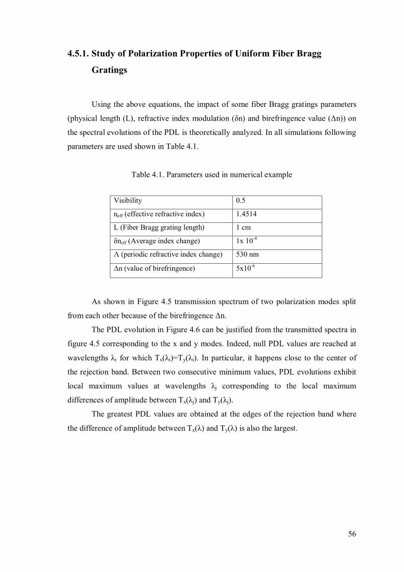
56
4.5.1. Study of Polarization Properties of Uniform Fiber Bragg
Gratings
Using the above equations, the impact of some fiber Bragg gratings parameters
(physical length (L), refractive index modulation (δn) and birefringence value (Δn)) on
the spectral evolutions of the PDL is theoretically analyzed. In all simulations following
parameters are used shown in Table 4.1.
Table 4.1. Parameters used in numerical example
Visibility 0.5
neff (effective refractive index) 1.4514
L (Fiber Bragg grating length) 1 cm
δneff (Average index change) 1x 10⁻⁴
Λ (periodic refractive index change) 530 nm
Δn (value of birefringence) 5x10⁻⁶
As shown in Figure 4.5 transmission spectrum of two polarization modes split
from each other because of the birefringence Δn.
The PDL evolution in Figure 4.6 can be justified from the transmitted spectra in
figure 4.5 corresponding to the x and y modes. Indeed, null PDL values are reached at
wavelengths λi for which Tx(λi)=Ty(λi). In particular, it happens close to the center of
the rejection band. Between two consecutive minimum values, PDL evolutions exhibit
local maximum values at wavelengths λj corresponding to the local maximum
differences of amplitude between Tx(λj) and Ty(λj).
The greatest PDL values are obtained at the edges of the rejection band where
the difference of amplitude between Tx(λ) and Ty(λ) is also the largest.

57
Figure 4.5. Evolution of transmission coefficient of a uniform fiber Bragg grating
Figure 4.6. Polarization Dependent Loss of a uniform fiber Bragg grating
As shown on these figures 4.7, 4.8, 4.9, 4.10, the grating length and the
refractive index modulation have similar effect on the PDL spectra, which is an increase
of the peak amplitudes at wavelengths coinciding with the edges of the rejection band of
the transmitted spectrum.
1538 1538.1 1538.2 1538.3 1538.4 1538.5 1538.6 1538.7 1538.8 1538.9 15390
0.1
0.2
0.3
0.4
0.5
0.6
0.7
0.8
0.9
1
Wavelength (nm)
TFB
Gx
TFB
Gy
TxTy
1538 1538.1 1538.2 1538.3 1538.4 1538.5 1538.6 1538.7 1538.8 1538.9 15390
0.2
0.4
0.6
0.8
1
1.2
1.4
Wavelength (nm)
PD
L (d
B)

58
The transmitted spectrum is characterized by an increasing amplitude variation
at the edges of the main rejection band whereas the wavelength spacing between the
two polarization modes is slightly influenced. As a result, sharp PDL evolutions with
important maximum values in the rejection band are obtained for gratings characterized
by long physical lengths and/or high refractive index modulations.
In figures, the curves are obtained as a function of the normalized wavelength.
Normalized wavelength is defined as the ratio between the working wavelength and the
central wavelength λmax (λ /λmax).
Figure 4.7. Transmitted spectrum evolution as a function of grating length
Figure 4.8. Polarization Dependent Loss spectra as a function of grating length
0.9996 0.9997 0.9998 0.9999 1 1.0001 1.0002 1.00030
0.1
0.2
0.3
0.4
0.5
0.6
0.7
0.8
0.9
1
Normalized Wavelength
T
L=0.4cmL=0.8cmL=1.2cmL=1.6cm
0.9996 0.9997 0.9998 0.9999 1 1.0001 1.0002 1.00030
0.5
1
1.5
2
2.5
3
3.5
4
Normalized Wavelength
PDL(
dB)
L=0.4cmL=0.8cmL=1.2cmL=1.6cm

59
Figure 4.9. Transmitted spectrum evolution as a function of grating periodicity
Figure 4.10. Polarization Dependent Loss spectra as a function of grating periodicity
0.9998 0.9999 1 1.0001 1.00020
0.1
0.2
0.3
0.4
0.5
0.6
0.7
0.8
0.9
1
Normalized Wavelength
T
n = 1 x 10⁻⁴
n = 2 x 10⁻⁴
n = 3 x 10⁻⁴
n = 4 x 10⁻⁴
0.9998 0.9999 1 1.0001 1.00020
0.2
0.4
0.6
0.8
1
1.2
1.4
1.6
Normalized Wavelength
PD
L(dB
)
n = 1 x 10⁻⁴
n = 2 x 10⁻⁴
n = 3 x 10⁻⁴
n = 4 x 10⁻⁴

60
Figure 4.11. Transmitted spectrum evolution as a function of birefringence value
Figure 4.12. Polarization Dependent Loss spectra as a function of birefringence value
0.9996 0.9997 0.9998 0.9999 1 1.0001 1.0002 1.00030.1
0.2
0.3
0.4
0.5
0.6
0.7
0.8
0.9
1
Normalized Wavelength
T
n = 0.2 x 10⁻⁴
n = 0.6 x 10⁻⁴
n = 1 x 10⁻⁴
n = 1.4 x 10⁻⁴
n = 1.8 x 10⁻⁴
0.9996 0.9997 0.9998 0.9999 1 1.0001 1.0002 1.00030
1
2
3
4
5
6
7
8
9
Normalized Wavelength
PD
L(dB
)
n = 0.2 x 10⁻⁴
n = 0.6 x 10⁻⁴
n = 1 x 10⁻⁴
n = 1.4 x 10⁻⁴
n = 1.8 x 10⁻⁴

61
CHAPTER 5
INTERROGATION OF POLARIZATION EFFECTS
IN FBG BY USING OFDR
5.1. Introduction
In this chapter, in order to understand whether the polarization properties of
uniform FBGs may be interrogated by the way of OFDR, a numerical simulation model
is built for the OFDR system where the FBG is modeled by implementing the transfer
matrix method. This model takes into account the effect of birefringence on the FBG’s
spectral response. Once the signal on the photodetector of the OFDR is modeled, the
signal processing steps (based on FFT and IFFT), as explained in chapter 3, are used in
order to obtain (“demodulate”) the transmission spectrum responses of the FBG.
Finally, based on the demodulated transmission spectra for both polarization modes,
Polarization Dependent Loss of the FBG is determined.
5.2. Numerical Simulation Model of OFDR System Considering Two
Polarization Modes
Figure 5.1 represents the distributed sensing system containing C-OFDR and
FBG. The main difference from the model used in section 3.3.2.2 is that two transfer
matrices are assigned to each small section of the FBG [54]. Therefore, it is allowed to
obtain Bragg spectra at an arbitrary position for given birefringence value.

62
Figure 5.1. Model of FBG and mirror on C-OFDR system with two polarization modes (TLS: Tunable Laser Source, PD: Photodedector, C: Coupler)
As shown in Figure 5.1 the tunable laser source sweeps the wavelength λ of the
incident light. This probe signal is split at the coupler C1 into mirror and test arms.
Reflected light from mirror and FBG interfere and observed at the detector (D1).
The distributed spectrum of the FBG at each position all along the grating length
can be obtained by applying Short Time Fourier Transform (STFT) on the detector
signal (D1).
A certain range of wavenumber is extracted by window function. Fast Fourier
transform is applied to the defined range to obtain the power profile of each frequency
component. By sliding window function through the whole wavenumber range and by
realizing proper conversions (wavenumber and frequency domains are converted to the
wavelength and position, respectively), a spectrogram is constructed which shows the
power profile along the FBG for each optical wavelength [55].
In the presence of birefringence, two grating matrices, phase shift matrices, and
input /output fields are assigned to two polarization modes.
TLS
PD
C1 Fiber Bragg Grating
D1
L
PBragg(x,y)
0 z0 z1
Pmirror(x,y)
Mirror
z2
z1 z2
FBx(1)
FBy(1)
FBx(2)
FBy(2)
FBx(3)
FBy(3)
…
…
…
…
…
…
…
…
…
…
…
…
FBx(N)
FBy(N)
Δz Δz Δz Δz

63
The elements of the grating matrices 퐹 ( …. ) (j=x or y) are formed in equations
5.1, 5.2, 5.3, 5.4 as,
T = cosh α L − ( ) (5.1)
T =− κ ( ) (5.2)
T = κ ( ) (5.3)
T = cosh α L + ( ) (5.4)
퐹 =cosh α Δz − − κ
κ ( ) cosh α Δz + ( ) (5.5)
The phase shift matrices PMj and PBj (j=x or y) of the reflection matrices of two
polarization modes are calculated as,
푃 = 푒ø
0
0푒ø (5.6)
ø = 푛 , 푧 (5.7)
In the case of mirror side of the optical path, the relation between output and
input of the system is given as,
푅 (0)푆 (0) = 푃
푅 (푧 )푆 (푧 ) (5.8)
where RMj is the amplitude of the forward propagation mode, SMj is the amplitude of the
backward propagating mode and PMj is the mirror phase shift matrix.
The phase shift matrix PMj of the mirror is given as,
푃 = 푒ø
0
0푒ø (5.9)
ø = 푛 , 푧 (5.10)

64
When the boundary conditions are applied,
푅 (0) = 1 (5.11)
푆 (푧 ) = 푅 (푧 )푒 (5.12)
1
푆 (0) =푃 푃푃 푃
푅 (푧 )푅 (푧 )푒
(5.13)
The mirror reflection coefficient is given as,
푅퐿 = 푆 (0).풙 + 푆 (0).풚
= .풙 + . 풚 (5.14)
For the optical path contains fiber Bragg grating, the transfer matrix (Tj) for the
whole optical path is considered as the multiplication of the transfer matrices of all the
individual FBG sections and express as,
푇 = 푃 퐹 ( ) ……퐹 ( )퐹 ( ) (5.15)
where PBj (j=x or y) is Bragg phase shift matrix and given as,
푃 = 푒ø
0
0푒ø (5.16)
ø = 푛 , 푧 (5.17)
The relation between input and output of the Bragg system for the two
polarization mode is defined by the equation 5.18,
푅 (0)푆 (0) = 푇
푅 (푧 )푆 (푧 ) (5.18)
where RBj is the amplitude of the forward propagating mode and SBj is the amplitude of
the backward propagating modes.

65
The boundary conditions for the Bragg system will be defined as,
푅 (0) = 푎 푒 (5.19)
푅 (0) = 푎 푒 (5.20)
푆 (푧 ) = 0 (5.21)
푆 (푧 ) = 0 (5.22)
where the amplitude and the phase of the two polarization state are expressed as aj and
φj (j=x or y), respectively,
When the boundary condition is applied on equation 5.18, the reflection
coefficient for Bragg grating can be obtained as,
푅퐿 = 푆 (0). 풙 + 푆 (0). 풚
= 푎 푒 . 풙 + 푎 푒 . 풚 (5.23)
The transmission coefficient of the Bragg grating is obtained as,
푇 = 푅 (푧 ). 풙 + 푅 (푧 ). 풚
= 푎 푒 . 풙 + 푎 푒 . 풚 (5.24)
The obtained detector signal can be expressed as,
퐷 = |푅퐿 + 푅퐿 | (5.25)
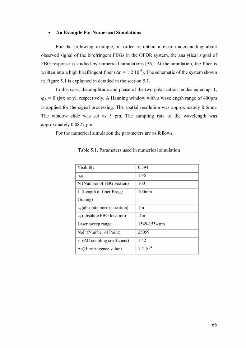
66
An Example For Numerical Simulations
For the following example, in order to obtain a clear understanding about
observed signal of the birefringent FBGs in the OFDR system, the analytical signal of
FBG response is studied by numerical simulations [56]. At the simulation, the fiber is
written into a high birefringent fiber (Δn = 1.2 10-4). The schematic of the system shown
in Figure 5.1 is explained in detailed in the section 5.1.
In this case, the amplitude and phase of the two polarization modes equal aj= 1,
휑 = 0 (j=x or y), respectively. A Hanning window with a wavelength range of 400pm
is applied for the signal processing. The spatial resolution was approximately 0.6mm.
The window slide was set as 5 pm. The sampling rate of the wavelength was
approximately 0.0827 pm.
For the numerical simulation the parameters are as follows,
Table 5.1. Parameters used in numerical simulation
Visibility 0.394
neff 1.45
N (Number of FBG section) 100
L (Length of fiber Bragg
Grating)
100mm
z0 (absolute mirror location) 1m
z1 (absolute FBG location) 4m
Laser sweep range 1549-1554 nm
NoP (Number of Point) 25059
κ (AC coupling coefficient) 1.42
Δn(Birefringence value) 1.2 10-4

67
In Figure 5.2 and 5.3 reflection amplitude of x and y polarization modes and
power of detector signal (D1) are presented where the split between the two polarization
modes is equal to 240pm.
Figure 5.2. Evolution of reflection spectrum of two polarization mode
1549.95 1550 1550.05 1550.1 1550.15 1550.2 1550.25 1550.3
0
2
4
6
8
10
12
14
16
18
x 10-3 Fbg reflection spectrum versus lambda
Wavelength(nm)
Ref
lect
ion
Am
plitu
de
-Reflectivity of x mode--Reflectivity of y mode

68
Figure 5.3. Evolution of detector signal
Figure 5.4. Simulated beat spectrum converted to distance scale
Simulated beat spectrum of the photodetector can be seen from the Figure 5.4.
Intensity detected by the photodetector in above explained system is a wavenumber
dependent sinusoidal function with a constant frequency called beat frequency. The beat
frequency can be expressed as,
훥푘 = (5.26)
1549 1549.5 1550 1550.5 1551 1551.50.75
0.8
0.85
0.9
0.95
1
Wavelength(nm)
Out
put S
igna
l Pow
er(a
.u.)
2.95 3 3.05 3.1 3.150
1
2
3
4
5
6
7
8x 10⁻³
Position(m)
Det
ecte
d Sig
nal(a
.u.)
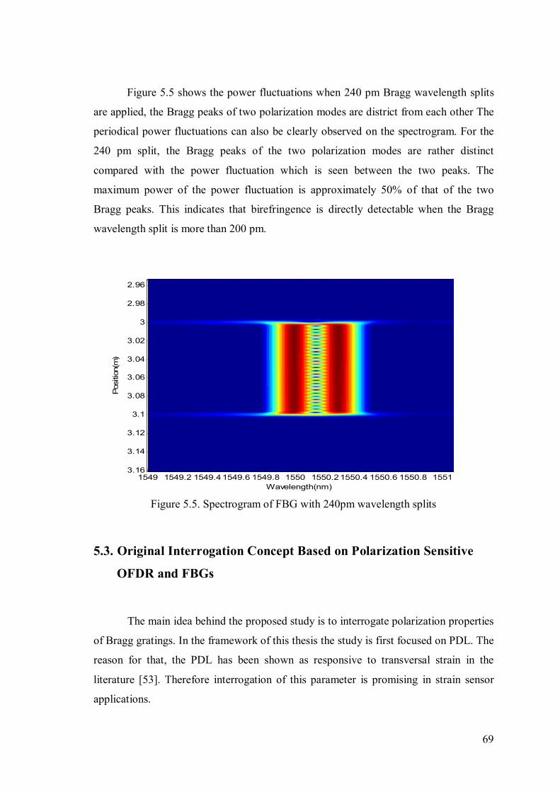
69
Figure 5.5 shows the power fluctuations when 240 pm Bragg wavelength splits
are applied, the Bragg peaks of two polarization modes are district from each other The
periodical power fluctuations can also be clearly observed on the spectrogram. For the
240 pm split, the Bragg peaks of the two polarization modes are rather distinct
compared with the power fluctuation which is seen between the two peaks. The
maximum power of the power fluctuation is approximately 50% of that of the two
Bragg peaks. This indicates that birefringence is directly detectable when the Bragg
wavelength split is more than 200 pm.
Figure 5.5. Spectrogram of FBG with 240pm wavelength splits
5.3. Original Interrogation Concept Based on Polarization Sensitive
OFDR and FBGs
The main idea behind the proposed study is to interrogate polarization properties
of Bragg gratings. In the framework of this thesis the study is first focused on PDL. The
reason for that, the PDL has been shown as responsive to transversal strain in the
literature [53]. Therefore interrogation of this parameter is promising in strain sensor
applications.
Wavelength(nm)
Pos
ition
(m)
1549 1549.2 1549.41549.6 1549.8 1550 1550.21550.4 1550.6 1550.8 1551
2.96
2.98
3
3.02
3.04
3.06
3.08
3.1
3.12
3.14
3.16
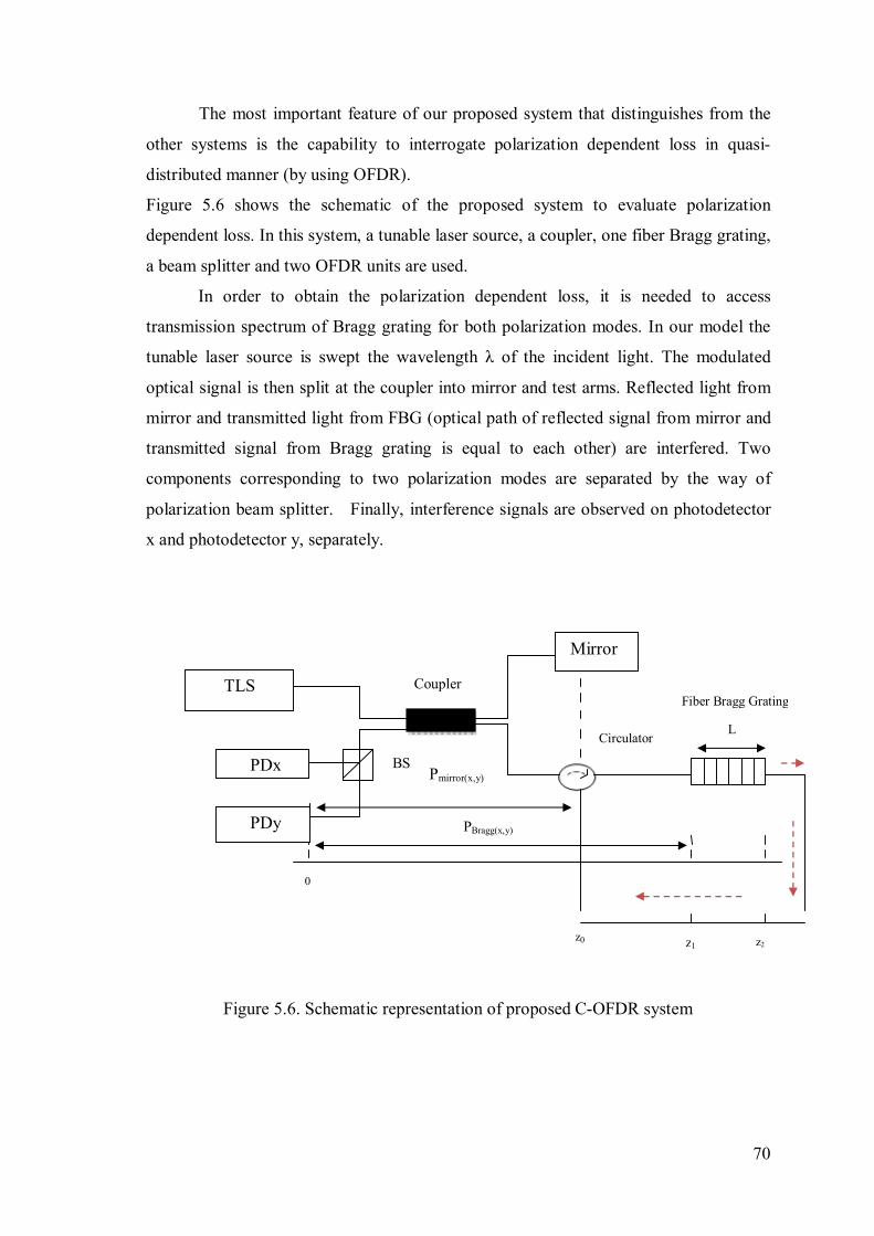
70
The most important feature of our proposed system that distinguishes from the
other systems is the capability to interrogate polarization dependent loss in quasi-
distributed manner (by using OFDR).
Figure 5.6 shows the schematic of the proposed system to evaluate polarization
dependent loss. In this system, a tunable laser source, a coupler, one fiber Bragg grating,
a beam splitter and two OFDR units are used.
In order to obtain the polarization dependent loss, it is needed to access
transmission spectrum of Bragg grating for both polarization modes. In our model the
tunable laser source is swept the wavelength λ of the incident light. The modulated
optical signal is then split at the coupler into mirror and test arms. Reflected light from
mirror and transmitted light from FBG (optical path of reflected signal from mirror and
transmitted signal from Bragg grating is equal to each other) are interfered. Two
components corresponding to two polarization modes are separated by the way of
polarization beam splitter. Finally, interference signals are observed on photodetector
x and photodetector y, separately.
Figure 5.6. Schematic representation of proposed C-OFDR system
TLS
PDx
Coupler Fiber Bragg Grating
L
PBragg(x,y)
0
z0 z1
Pmirror(x,y)
z2
PDy
BS
Mirror
Circulator

71
By using equations obtained in section 5.2, output signals calculated at detector
x and detector y can be provided.
In the reference arm of the system reflected light from the mirror is calculated
as,
푅퐿 , = .풙 (5.27)
푅퐿 , = . 풚 (5.28)
where 푃 and 푃 are the phase shift matrix for the optical path contains mirror.
푃 = 푒 ( , )00푒( , )
(5.29)
For the optical path with FBG, transmitted light is calculated with respected
boundary conditions in section 5.2 as,
푇 , = 푎 푒 . 풙 (5.30)
푇 , = 푎 푒 . 풚 (5.31)
where 푎 , 휑 (j=x or y) are the amplitude and phase of the polarization state of the
input signal and 푇 denotes the elements of transfer matrix , Tj.
Finally the output signal can be expressed by taking the absolute square of
coupled signals reflected from reference path and transmitted from test path. The
obtained signal Dx and Dy were calculated as,
퐷 = 푅퐿 , + 푇 , (5.32) 퐷 = 푅퐿 , + 푇 , (5.33)

72
Demodulation of Transmission Spectra
The OFDR spectrum is obtained applying Fast Fourier transform (as explained
in chapter 3) on the interference signals and power profile of the frequency component
converted to the corresponding distance of fiber Bragg grating.
In order to determine the demodulated transmission spectrum, inverse Fast
Fourier transform steps (as represented at the chapter 3) are applied around the
particular position of FBG by defining a proper window around beat frequency as
shown in Figure 5.7.
Figure 5.7. Demodulation scheme for the transmitted spectra
Extracted transmission evolution from demodulation allows computing
polarization dependent loss.
푃퐷퐿 = 10 log ( )( )
(5.34)
푇 , (휆) = 퐷푒푚표푑푢푙푎푡푒푑푃표푤푒푟푇푟푎푛푠푚푖푠푠푖표푛퐶표푒푓푓푖푐푖푒푛푡푠 (5.35)
OFDR
IFFT
OFDR trace
λB λB λB
Demodulated
Transmission
spectra
FBG1 FBG2 FBGN
frequency
Strain
Δλ
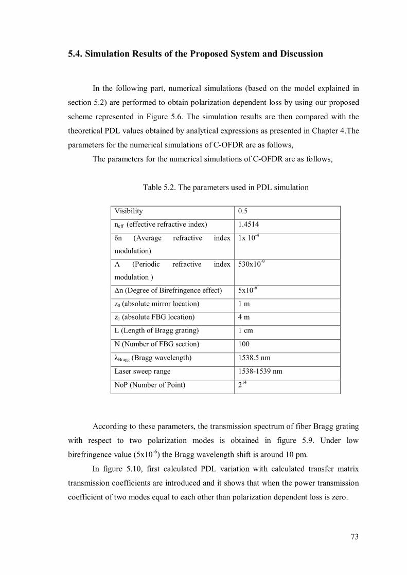
73
5.4. Simulation Results of the Proposed System and Discussion
In the following part, numerical simulations (based on the model explained in
section 5.2) are performed to obtain polarization dependent loss by using our proposed
scheme represented in Figure 5.6. The simulation results are then compared with the
theoretical PDL values obtained by analytical expressions as presented in Chapter 4.The
parameters for the numerical simulations of C-OFDR are as follows,
The parameters for the numerical simulations of C-OFDR are as follows,
Table 5.2. The parameters used in PDL simulation
Visibility 0.5
neff (effective refractive index) 1.4514
δn (Average refractive index
modulation)
1x 10⁻⁴
Λ (Periodic refractive index
modulation )
530x10-9
Δn (Degree of Birefringence effect) 5x10⁻⁶
z0 (absolute mirror location) 1 m
z1 (absolute FBG location) 4 m
L (Length of Bragg grating) 1 cm
N (Number of FBG section) 100
λBragg (Bragg wavelength) 1538.5 nm
Laser sweep range 1538-1539 nm
NoP (Number of Point) 214
According to these parameters, the transmission spectrum of fiber Bragg grating
with respect to two polarization modes is obtained in figure 5.9. Under low
birefringence value (5x10⁻⁶) the Bragg wavelength shift is around 10 pm.
In figure 5.10, first calculated PDL variation with calculated transfer matrix
transmission coefficients are introduced and it shows that when the power transmission
coefficient of two modes equal to each other than polarization dependent loss is zero.

74
Between two successive minimum values of power transmission coefficient the
polarization dependent loss takes its maximum values at the corresponding wavelength.
Second part of the figure 5.10 shows us the polarization dependent loss, calculated by
power transmission coefficient achieved after demodulation process this result is
matching with the calculated results.
As a result, a fiber Bragg grating transmission spectrum is demodulated and the
polarization dependent information is extracted by demodulating OFDR signal.
Figure 5.8. OFDR trace in frequency domain (converted into position)
2.97 2.98 2.99 3 3.01 3.02 3.03 3.04 3.05 3.06 3.070
0.2
0.4
0.6
0.8
1
1.2
1.4
1.6
1.8
Position(m)
Pow
er(a
.u.)

75
Figure 5.9. Transmitted spectrum of FBG for x and y modes
Figure 5.10. (a) PDL obtained by analytical calculations (b) simulated PDL
1538 1538.1 1538.2 1538.3 1538.4 1538.5 1538.6 1538.7 1538.8 1538.9 15390.4
0.5
0.6
0.7
0.8
0.9
1
Wavelength(nm)
Tran
smis
sion
Am
plitu
de
-Transmission of x mode--Transmission of y mode
1538.2 1538.3 1538.4 1538.5 1538.6 1538.7 1538.80
0.5
1
1.5
Wavelength(nm)
PD
L(dB
)
1538.2 1538.3 1538.4 1538.5 1538.6 1538.7 1538.80
0.5
1
1.5
Wavelength(nm)
Dem
odul
ated
PD
L(dB
)
(a)
(b)

76
After that impact of Bragg grating parameters as length (L), periodic refractive
index modulation (δn), and birefringence value on the spectral evaluation of
polarization dependent loss is performed.
Figure 5.11. Computed transmission spectrum of x and y mode as a function of grating length
Figure 5.12. (a) PDL obtained by analytical calculations (b) simulated PDL as a
function of grating length ()
1538 1538.1 1538.2 1538.3 1538.4 1538.5 1538.6 1538.7 1538.8 1538.9 15390.1
0.2
0.3
0.4
0.5
0.6
0.7
0.8
0.9
1
Wavelength(nm)
Tra
nsm
issi
on S
pect
rum
of x
-y m
ode
L =0.4cmL=0.8cmL=1.2cmL=1.6cm
1538.2 1538.3 1538.4 1538.5 1538.6 1538.7 1538.80
1
2
3
4
Wavelength(nm)
PD
L (O
rigin
al)(d
B)
L= 0.4 cmL= 0.8 cmL= 1.2 cmL= 1.4 cm
1538.2 1538.3 1538.4 1538.5 1538.6 1538.7 1538.80
1
2
3
4
Wavelength(nm)
PD
L(O
FDR
)(dB
)
L= 0.4 cmL= 0.8 cmL= 1.2 cmL= 1.4 cm
(a)
(b)

77
Figure 5.13. Computed transmission spectrum of x and y mode as a function of refractive index modulation
Figure 5.14. (a) PDL obtained by analytical calculations (b) simulated PDL as a
function of refractive index modulation
1538 1538.1 1538.2 1538.3 1538.4 1538.5 1538.6 1538.7 1538.8 1538.9 15390
0.1
0.2
0.3
0.4
0.5
0.6
0.7
0.8
0.9
1
Wavelength(nm)
Tra
nsm
issi
on S
pect
rum
of x
-y m
ode
n = 1 x 10⁻⁴
n = 2 x 10⁻⁴
n = 3 x 10⁻⁴
n = 4 x 10⁻⁴
1538.2 1538.3 1538.4 1538.5 1538.6 1538.7 1538.80
0.5
1
1.5
2
Wavelength(nm)
PD
L (O
rigin
al)(d
B)
n = 1 x 10⁻⁴
n = 2 x 10⁻⁴
n = 3 x 10⁻⁴
n = 4 x 10⁻⁴
1538.2 1538.3 1538.4 1538.5 1538.6 1538.7 1538.80
0.5
1
1.5
2
Wavelength(nm)
PD
L(O
FDR
)(dB
)
n = 1 x 10⁻⁴
n = 2 x 10⁻⁴
n = 3 x 10⁻⁴
n = 4 x 10⁻⁴
(a)
(b)
78
The evolution of the transmitted spectrum and PDL with respect to the grating
length is investigated in Figure 5.11 and 5.12. Figure 5.13 and 5.14 present the same
evolution with respect to the refractive index modulation. The parameters used in the
simulations are given in table 5.2.
As shown on figures, grating length and the refractive index modulation results
in the same effect on polarization dependent loss spectra. The peak amplitude is
increased at the wavelength coincidence with the edge of the rejection band of
transmitted spectra. For the long grating length and high refractive index modulation
values, sharp PDL evolution with maximum values in the rejection band is obtained.
The results obtained by analytical calculations is in a good agreement with the
results obtained after the demodulations process for grating length variation, refractive
index modulation and birefringence value variation.
The effect of the birefringence value is studied in Figure 5.15 and 5.16. For Δn
values less than 1 10−4 which corresponds to photo-induced birefringence values, the
birefringence effect is not well perceived in the transmitted spectrum as the two
transmitted spectra corresponding to the x and y modes is not split well enough. For the
Δn value bigger than 1.5 10-4 the split between the two spectra can be observed and the
amplitude remains unchanged.
For Δn values up to 1x10⁻⁴, the maximum PDL values monotonically increase whereas
the wavelength spacing between them slightly decreases. For Δn higher than 1x10⁻⁴, the
maximum PDL saturate but the wavelength spacing between the peaks is increased.

79
Figure 5.15. Computed transmission spectrum of x and y mode as a function of birefringence value
Figure 5.16. (a) PDL obtained analytical calculations (b) simulated PDL as a function of birefringence value
1538 1538.1 1538.2 1538.3 1538.4 1538.5 1538.6 1538.7 1538.8 1538.9 15390.5
0.55
0.6
0.65
0.7
0.75
0.8
0.85
0.9
0.95
1
Wavelength(nm)
Tra
nsm
issi
on S
pect
rum
of x
-y m
ode
n = 0.2 x 10⁻⁴
n = 0.6 x 10⁻⁴
n = 1 x 10⁻⁴
n = 1.4 x 10⁻⁴
n = 1.8 x 10⁻⁴
1538.2 1538.3 1538.4 1538.5 1538.6 1538.7 1538.80
5
10
Wavelength(nm)
PD
L (O
rigin
al)(d
B)
n = 0.2 x 10⁻⁴
n = 0.6 x 10⁻⁴
n = 1 x 10⁻⁴
n = 1.4 x 10⁻⁴
n = 1.8 x 10⁻⁴
1538.2 1538.3 1538.4 1538.5 1538.6 1538.7 1538.80
5
10
Wavelength(nm)
PD
L(O
FDR
)(dB
)
n = 0.2 x 10⁻⁴
n = 0.6 x 10⁻⁴
n = 1 x 10⁻⁴
n = 1.4 x 10⁻⁴
n = 1.8 x 10⁻⁴
(a)
(b)

80
Discussion
Birefringence in fiber Bragg gratings can be produced by combining the intrinsic
birefringence with the birefringence induced by UV writing process or birefringence
induced by transversal load can [1], [2]. As shown in Figures 5.15 and 5.16,
birefringence leads to polarization dependent loss in fiber Bragg gratings. Furthermore
when a grating is subjected to transversal load, this effect leads to a modification in
PDL evolution. Because birefringence value variation depends on applied transversal
load. [2]
The transversal load effect is studied in literature as shown in Figure 5.17 that
less than 250 N transversal force value can be measured based on monitoring PDL
evolution. The result of the figure can be associated with figure 5.16 that after 1x10⁻⁴
birefringence value PDL amplitudes saturate and amplitude of PDL can’t answer the
load variation.
Figure 5.17. Evolution of maximum PDL value as a function of the measured transverse force value and reconstructed birefringence value [2]
The PDL evolution results of literature are good agreement with the presented
study and show that the proposed approach in this thesis can be used to monitor
transversal load on the structure in distributed or quasi-distributed manner.

81
CHAPTER 6
CONCLUSIONS
The goal of this thesis is to demonstrate the feasibility of an original fiber Bragg
grating interrogation scheme which is able to obtain polarization properties of FBGs by
using OFDR.
A theoretical model has been introduced and numerical simulations have been
carried out to study the responses of uniform fiber Bragg grating interrogated by OFDR.
In first chapter of the thesis, fundamentals of fiber Bragg gratings are studied.
The effect of grating parameters (length, grating period,...) on the reflection spectrum is
analyzed using analytical formulas.
In the second chapter of the thesis, the state of the art covering various FBG
interrogation methods is briefly presented. Optical Frequency Domain Reflectometry
comes out to be a suitable technique for quasi-distributed sensor applications envisaged
by this thesis. Therefore, after giving basic principles of OFDR, this chapter includes a
mathematical analysis together with the numerical simulations of an OFDR system
where a single FBG is used as the sensing element.
In chapter four, preliminary studies have been conducted in order to include the
effect of the birefringence in the proposed model. Spectrograms have been obtained to
study the power distribution along the FBG while taking both the polarization state of
the input light beam and the birefringence of the FBG into consideration.
Chapter five contains the main added-value of the thesis. In this chapter, we
propose an original scheme to interrogate PDL of a number of cascaded FBGs by the
way of polarization sensitive OFDR. Then, we analyzed the PDL of the FBGs by the
way of numerical simulations. Our simulation results have shown a very good
agreement with the theoretical results.
In conclusion, our model and analysis have revealed the feasibility of an original
scheme which is able to interrogate polarization dependent loss by optical frequency
domain reflectometer.
The results provide an important guidance in designing novel fiber optic sensors
utilizing fiber gratings as the sensing element and OFDR as the interrogation unit.
82
Perspectives
The results of the thesis open the door to an interesting application area, namely
strain sensors monitoring composite materials. The use of optical fiber sensing,
particularly embedding of fiber Bragg grating (FBG) sensors into composite materials
has been gaining growing popularity thanks to various advantages of FBGs. For the
development of smart structures, fiber Bragg gratings brought about a great
contribution in many engineering fields (civil, aerospace, renewable energy, …).
The use of composite materials in critical parts and high stress members
(airplane wings, unmanned air vehicles, wind turbines…) has been exponentially
growing thanks to their lightweight, superior strength, durability, and corrosion
resistance. However, the unique mechanical properties of composite materials cannot be
fully exploited without monitoring them when material is placed under constraints. This
is because the behavior of composite materials under loading is different from metals
and can rapidly degrade when internal damage occurs. It is therefore essential to
monitor their behavior in the field or during manufacturing and prototyping for the
purpose of improved performance, improved safety, and reduced cost.
The occurrence and growth of damage in composite elements can be detected by
continually measuring the mechanical load, stress and strain inside the structures.
More than tens of fiber Bragg gratings can be cascaded in a single fiber. By
combining the cascaded capability and compatibility with composite materials, optical
fiber Bragg grating sensors are well suited to be embedded into composite materials
without reforming their physical properties.
In literature, sensitivity of polarization properties of FBG to the transversal
strain is demonstrated in recent publications [3] [4]. However, none of the previously
demonstrated reports using FBG sensors could exhibit quasi-distributed or distributed
measurement capability which significantly limits their implementations into composite
materials. The novel interrogation technique that we proposed in this thesis can be
implemented in many applications related to the strain monitoring of composite
materials.

83
REFERENCES
[1] Erdoğan T., “Fiber grating spectra,’’ Journal of Lightwave Technology, vol. 15, num. 8, pp. 1277–1294, 1997.
[2] Caucheteur C., “Realization of mechanical and chemical sensors based on the fiber Bragg gratings technology,’’ Faculté Polytechnique de Mons, 2007.
[3] Zhang P., “High-resolution photon counting OTDR based interrogation of multiplexing broadband FBG sensors,’’ PhD Dissertation Electrical and Computer Engineering Department, Blacksburg, Virginia, USA, 2003.
[4] Voisin V., Caucheteur C., Kinet D., Mégret P., Wuilpart M., “ Self-referenced Photon Counting OTDR Technique for Quasi-distributed Fiber Bragg Gratings Sensors,’’ IEEE Sensors Journal, 12, pp. 118-123, 2012.
[5] Fidanboylu K., Efendioğlu H. S., “Fiber optic sensors and their applications,’’ 5th International Advanced Technologies Symposium (IATS’09), Karabük, Turkey, May 13-15, 2009.
[6] Francis To, So Yu, Shizhuo Yin, “Optical fiber sensors guide, Fundamentals & Applications,’’ Micron Optics, August 22, 2009.
[7] Saleh B.E.A., Teich M.C., “Fundamentals of Photonics,’’ Wiley & Sons, 2007.
[8] Yariv A., “Quantum Electronics,’’ Wiley& Sons, 1989.
[9] Hartog H. A., “Distributed fiber optic sensors, Optical Fiber Sensor Technology,’’ Chapman and Hall, London, 1995.
[10] Glisic B., “Distributed fiber optic sensing technologies and applications – an overview,’’ ACI Special Publication, SP-292, art. no. 2 (18pp), 2013.
[11] Yu T. S. F., Yin S., “Fiber Optic Sensors,’’ Pennsylvania State University, Pennsylvania, ISBN: 0-8247-0732-X, 2002.
[12] Othonos A., Kalli K., “Fiber Bragg gratings: Fundamentals and applications in telecommunications and sensing,’’ Artech House, 1999.
[13] Kashyap R., “Fiber Bragg Gratings,’’ 1990.

84
[14] Roths J., Sudan C., Kuttler R., Gerz C., “High Precision, Low-Cost Interrogation System for Fiber Bragg Grating Sensors,’’ Munich University of Applied Sciences, DGaO Proceedings, 2005.
[15] Kreuzer M., “Strain measurement with fiber Bragg grating sensors,’’ HBM, Darmstadt, Germany, HBM, Darmstadt, Germany, 2007.
[16] Smartfibres [website]. Avaible: www.smartfibres.com.
[17] Durana G., Kirchhof M., Luber M., Ocáriz I. S., Poisel H., Vázquez C., Zubia J., “Use of a Novel Fiber optical strain sensor for monitoring the vertical deflection of an Aircraft flap,’’ IEEE Sensors Journal, Vol. 9, No. 10, 2009.
[18] Mishra V., Singh N., “Optical fiber gratings in perspective of their applications in Biomedicine,’’ Central Scientific Instruments Organization, (CSIR), New Delhi, 2011. [19] Glavind L., Olesen I., Skipper B., Kristensen M., “Fiber-optical grating sensors for wind turbine blades: a review,’’ SPIE, Optical Engineering 52(3), 030901, 2013.
[20] Filograno M. L., Corredera P., Rodríguez-Barrios A., Martín-López S., Rodríguez-Plaza M., Andrés-Alguacil A., González-Herráez M., “Real time monitoring of railway traffic using fiber Bragg grating sensors,’’ IEEE Sensors J. 12(1), 85–92 (2012).
[21] Vendittozzi C., Sindoni G., Paris C., Marmo P. P., “Application of an FBG sensors system for structural health monitoring and high performance trimming on racing yacht,’’ Fifth International Conference on Sensing Technology, 2011. [22] Lan Yi, “Geothermal Power Plant Monitoring Using FBG Temperature Sensors,’’ A Micron Optics Case Study, Taiwan, 2012.
[23] Melle S., Liu K., Measure R., “A passive wavelength demodulation system for guided wave Bragg grating strain sensor,’’ IEEE Photonics Technology Letters, vol. 4, no.5, pp.516-518, 1992.
[24] Davis M., Kersey A., “All- fiber Bragg grating strain sensor demodulation technique using wavelength division coupler,’’ Electronics Letter, vol.30, no.1, pp. 75-77, 1994.
[25] Davis M., Kersey A., “Matched-filter interrogation technique for fiber Bragg grating arrays,’’ Electronics Letter, vol. 37, no. 70, 1995.
[26] Xu M.G., Geiger H., and Dakin J., “Modeling and performance analysis of a fiber Bragg grating interrogation system using an acousto-optic tunable filter,’’ Journal of Lightwave Technology, vol. 14, no. 3, 1996.

85
[27] Kersey A., Berkoff T., and Morey W., “Multiplexed fiber Bragg grating strain-sensor system with a Fabry-Perot wavelength filter,” Optics Letters, vol. 18, pp. 1370–1372, 1993.
[28] Kersey A., Berkoff T., and Morey W., “Fiber optic Bragg grating sensor with drift-compensated high resolution interferometric wavelength shift detection,” Optics Letters, vol. 18, issue 1, pp. 72–74, 1993.
[29] Beller, “OTDRs and backscatter measurements in fiber optic test and measurement,’’ Prentice Hall, 1998.
[30] Anderson R.D., Bell G.F., “Optical Time Domain Reflectometry- OTDR,’’ Tektonix, Inc, Willsonville, Oregon, 1997.
[31] Crunelle C., “Development of quasi-distributed and distributed fiber temperature sensors based on optical reflectometry techniques,’’ Faculté Polytechnique de Mons, 2007.
[32] Zhang P., Nunez H., Qi B., Pickrell G., and Wang A., “Optical time-domain reflectometry interrogation of multiplexing low-reflectance Bragg grating- based sensor system,’’ Optical Engineering, vol.42, no. 6, pp. 1597-1603, 2003.
[33] Valente B., Braga A., Ribeiro A., Regazzi R., Ecke W., Chojetzki C., and Willsh R., “Combined time and wavelength multiplexing technique of optical fiber grating arrays using commercial OTDR equipment,’’ IEEE sensors journal, vol.3, no.1, pp. 31-35, 2003.
[34] Eom T., Kim M., Lee B., and Park I., “Temperature monitoring system based on fiber Bragg grating arrays with wavelength tunable OTDR,’’ IEICE Trans. Electron., vol. E88, no. 5, pp.933-937, 2005.
[35] Zheng J., “Analysis of optical frequency-modulated continuous-wave interference,’’ Applied Optics, vol.43, no.21, pp. 4189-4197, 2004.
[36] Derickson D., Fiber Optic Test and Measurement, Prentice Hall PTR, 1998.
[37] Yüksel K., “Development of an optical frequency domain reflectometer and applications to the interrogation of fiber Bragg gratings,’’ Faculté Polytechnique de Mons, 2011.
[38] Childers B., Froggatt M., Allison S., Moore T., Hare D., Batten C., Jegley D., “Use of 3000 Bragg grating strain sensors distributed on four eight-meter optical fibers during static load test of a composite structure,’’ Proceeding of SPIE vol. 4332, 2001.

86
[39] Duncan R., Childers B., Gifford D., Pettit D., Hickson A., and Brown T., “Distributed sensing technique for test article damage detection and monitoring,’’ Proceeding of SPIE Fiber Optic and Laser Sensors XIV conference, 2002.
[40] Abdi A., “Structural monitoring with fiber Bragg grating strain sensor array and optical frequency domain reflectometry,’’ The University of Arizona, 2005.
[41] Richard L., Parker A., Ko W., Piazza A., “Real time in flight strain and deflection monitoring with fiber optic sensors,’’ Space Sensor and Measurement Techniques Workshop, 2008.
[42] Igawa H., Ohta K., Kasai T., Yamaguchi I., Murayama H., Kageyama K., “Distributed Measurements with a long gauge FBG sensor using optical frequency domain reflectometry,’’ Journal of Solid Mechanics and Materials Engineering, vol. 2, no. 9, 2008.
[43] Hernday P., Fiber Optic Test and Measurement: Polarization Measurements, Chapter 6, Prentice Hall, N. J. 1998.
[44] Rogers A., Essentials of Optoelectronics, Chapman and Hall, 1993.
[45] Azzam R., Bashara N., Ellipsometry and Polarized Light, North- Holland, 1977.
[46] Kumar A., Ghatak A., “Polarization of light with applications in optical fibers,’’ Optical Engineering, v. TT90, 2011.
[47] Newport, “Polarization control and measurement for optical fibers,’’ Application Note, Spectra Physics, 2004
[48] Linze N., Wuilpart M., Tihon P., Verlinden O., “Design of an optical-fiber accelerometer based on polarization variation due to crushing of the fiber,’’ 10th International Conference on Vibration Problems, Springer Proceedings in Physics, Vol. 139, 2011.
[49] Belhadj N., LaRochelle S., Dossou K., “Form birefringence in UV exposed photosensitive fibers computed using a higher order finite element method,’’ Optics Express, vol. 12, pp. 1720–1726, 2004.
[50] Erdogan T., Mizrahi V., “Characterization of UV-induced birefringence in photosensitive Ge-doped silica optical fibers,’’ Journal of the Optical Society of America B, vol. 11, pp. 2100–2105, 1994.

87
[51] Bette S., Caucheteur C., Wuilpart M., Megret P., “Theoretical and experimental study of differential group delay and polarization dependent loss of Bragg gratings written in birefringent fiber,’’ Optical Communications, 269, pp. 331-337, 2007.
[52] Wuilpart M., Caucheteur C., Bette S., Megret P., Blondel M., “Polarization properties of uniform fiber Bragg gratings written in highly birefringent fibers.’’ Optical Communications, 247, pp. 239-245, 2005.
[53] Caucheteur C., Bette S., Olcina R., Wuilpart M., Sales S., Capmany J., Megret P., “Transversal strain measurements using the birefringence effect in fiber Bragg gratings.’’ IEEE Photonics Technology Letters, vol. 19, no. 13, 2007.
[54] Murayama H., Kageyama K., Uzawa K., Ohara K., and Igawa H., “Strain monitoring of a single-lap joint with embedded fiber-optic distributed sensors,’’ Structural Health Monitoring, 2011.
[55] Wada D., Murayama H., Kageyama K., Igawa H., Uzawa K., Omichi K., and “Simultaneous distributed measurement of strain and temperature by polarization maintaining fiber Bragg grating based on optical frequency domain reflectometry,’’ Smart Material Structures. 20, 2011.
[56] Wada D., Murayama H., “Analytical investigation of response of birefringent fiber Bragg grating sensors in distributed monitoring system based on optical frequency domain reflectometry.’’ Optics and Lasers in Engineering, 52, pp. 99–105, 2014.

88
APPENDIX A
COUPLE MODE THEORY
Let us consider a fiber Bragg grating formed within the core of an optical fiber
with an average refractive index ncore. The refractive index profile along the longitudinal
axis of the optical fiber z can be expressed as,
푛(푧) = 푛 (푧) + 훿푛(푧) 1 + 휈(푧)푐표푠 푧 + ø(푧) (A.1)
where
• δn (z) is the average refractive index modulation (typical values lie between
10−5 and 10−3);
• ν (z) represents the visibility of the interference fringes (0<v<1);
• Λ (z) is the periodicity of the refractive index modulation;
• ø (z) represents the phase variation inside the fiber grating.
Equation (A.1) allows to define different kinds of fiber gratings since the
amplitude, periodicity and phase of the refractive index modulation evolve along the
grating length.
In the ideal-mode approximation to coupled-mode theory, the transverse
component of the electric field assumed as a superposition of the ideal modes labeled j
(i.e., the modes in an ideal waveguide with no grating perturbation), so that
monochromatic wave equation is mathematically obtained as [1],
퐸⃗ (푥, 푦, 푧, 푡) = ∑ 퐴 (푧) exp(푖훽 ) + 퐵 (푧)exp(−푖훽 ) . 푒⃗ (푥, 푦)exp(−푖휔푡) (A.2)
where Aj(z) and Bj(z) are slowly varying amplitudes of the jth mode traveling in the +z
and –z directions, respectively. The transverse mode fields might describe the cladding
or radiation modes.

89
When the modes are orthogonal in an ideal waveguide, there do not occur
energy exchange, the presence of a dielectric perturbation causes the modes to be
coupled such that the amplitudes Aj and Bj of the jth mode evolve along the z axis:
= i∑ A (K + K )exp i β − β z
+i∑ B (K − K )exp −i β + β z (A.3)
= −i∑ A (K − K )exp i β + β z
−i∑ B (K + K )exp −i β − β z (A.4)
퐾 are the transverse coupling coefficients between modes j and k can be
calculated by using overlapping integrals:
K (z) = ∬ dxdy∆ε(x, y, z)푒⃗ (푥, 푦). 푒⃗∗ (푥, 푦) (A.5)
where ∆ε (x, y, z) is the perturbation of the electrical permittivity. Δϵ can be
approximated to 2ncoreδn when δn ≪ ncore. The longitudinal coefficients 퐾 (z)are
analogous to 퐾 but generally 퐾 (z) ≪퐾 (푧) for fiber modes so that these
coefficients are commonly neglected.
In most fiber gratings, the induced refractive index change is approximately
uniform across the core and zero outside the core. So the two coupling coefficient, σ
stands for the ’DC’ coupling coefficient (average over one period) and κ is the ’AC’
coupling coefficient are obtained as:
σ (z) = δn (z)∬ dxdy푒⃗ (푥, 푦). 푒⃗∗ (푥, 푦) (A.6)
κ (z) = σ (z) = δn (z)∬ dxdy푒⃗ (푥, 푦). 푒⃗∗ (푥, 푦) (A.7)
Thus the general coupling coefficient will be defined:
K (z) = σ (z) + 2κ (z)cos z + ø(z) (A.8)

90
By this theory, a series of differential equations of the first order presenting the
amplitude variation resultant of the mode coupling of the different modes propagating
along the optical fiber is obtained. For a uniform fiber Bragg grating which has uniform
and periodic perturbation has an analytical solution and occurs coupling between a
mode of amplitude A(z) and an identical mode propagating in the opposite direction of
amplitude B(z).
As a result of the calculations, the coupled mode theory gives following
equations:
= 푖휎푅(푧) + 푖κS(z) (A.9)
= −푖휎푆(푧) − 푖κR(z) (A.10)
Finally amplitudes R(z) and S(z) are defined as:
푅(푧) = 퐴(푧)exp(푖훿푧 − ø) (A.11)
푆(푧) = 퐵(푧)exp(−푖훿푧 + ø) (A.12)
In these equations the parameters are defined by the following relationships:
Self coupling coefficient σ = δ + σ (A.13)
AC coupling coefficient κ = πλ
υδn (A.14)
Tuning rate δ = β − πΛ= 2πn (
λ−
λ ) (A.15)
DC coupling coefficient σ = πλ
δn (A.16)
α = κ − σ (A.17)
For a uniform fiber Bragg grating, the parameters ˆσ, σ and κ do not depend on
the variable z. The system of differential equations is thus solved by specifying
appropriate boundary conditions. The first condition considers that the incident light is
normalized to 1 so that R(0)=1. The second condition sets S(z)=0 since the backward-
going wave does not exist further than the grating length L. With these two conditions,
the following results are obtained:

91
푅(푧) = 푅(0) cos(훼푧) + 푖 sinh(훼푧) + 푆(0)푖 κ sinh(훼푧) (A.18)
푆(푧) = 푆(0) cos(훼푧) − 푖 sinh(훼푧) − 푅(0)푖 κ sinh(훼푧) (A.19)
The amplitude evolution of the incident and reflected waves along the grating
can be presented in the matrix form as shown in equation A.20,
R(0)S(0) = T T
T T R(z)S(z) (A.20)
Elements of transfer matrix are determined as:
T = cosh(αL) − ( ) (A.21)
T =− κ ( ) (A.22)
T = κ ( ) (A.23)
T = cosh(αz) + ( ) (A.24)
These coefficients of the matrix will help us to determine reflection and
transmission coefficients belong to Bragg grating.

92
APPENDIX B
THEORY OF FMCW INTERFERENCE
Figure B.1 Basic C-OFDR scheme
As shown in figure probe signal is launched into the system and divided into two
optical path as reference and test arm [33].
The probe signal is a continuous wave coming from frequency modulated light
source and complex electric field of the probe signal can be expressed as,
E(t)=E0exp(jø(t)) (B.1)
where E0 is the amplitude of electric field and ø(t) is the phase component. The
conversion from time domain to wavenumber domain is started with the equation,
푡 = = 푧 (B.2)
where n is the effective refractive index of the optical fiber.
Laser
Detector
t
coupler
Local Oscillator
(Reference arm)
Device Under Test
(Test Arm)

93
The angular frequency which is the first derivative of phase component is
defined as,
휔(푡) = ø (B.3)
휔(푧) = ø (B.4)
Figure B.2. Test and reference signal interferency scheme
Using sawtooth-wave optical frequency modulated interference which affects
the beat term of the interference signal generates periodically ramped waveform due to
the two interfering wave’s optical frequency [35].
As the angular frequency of the probe signal’s optical frequency swept linearly
in time and can be expressed as,
휔(푡) = 2휋(훾 푡 + 휔 ) (B.5)
The angular frequency can be written as,
휔(푧) = 2휋(훾 + 휈 ) (B.6)
where ω0 is the initial angular frequency, ν0 is the initial optical frequency and γν is the
tuning rate in Hz/s and γk is the tuning rate in 1/m2.
γ = ; γ = (B.7)
z
λ
Zswp
References
Signal
Test Signal
kfinal
k0
Δz
Δvk
훾
0

94
where Tswp is the period of modulating signal in time domain and Zswp is the period by
means of distance.
So the phase component will be converted as,
ø(푡) = ∫ 휔(푢)푑푢 +ø (B.8)
ø(푧) = 2휋∫ 훾 푢 + 휈 푑푢 (B.9)
Finally the phase will be,
ø(푧) = 푧 훾 + 휈 푧 (B.10)
So the electric field of reflected signal from local oscillator (Eref(z)) is expressed
as,
퐸 (푧) = 퐸 exp 푗ø(푧) (B.11)
퐸 (푧) = 퐸 exp 푧 훾 + 휈 푧 (B.12)
The electrical field of reflected signal from device under test (from discrete
reflections- Etest(z)) is expressed as,
퐸 (푧) = 퐸 exp 푗ø(푧 − 퐿) (B.13)
퐸 (푧) = 퐸 exp (푧 − 퐿) 훾 + 휈 (푧 − 퐿) (B.14)

95
The intensity of interference signal computed at the detector is the sum of
individual electrical fields and can be defined as,
퐷(푧) = 퐸 (푧) + 퐸 (푧) (B.15)
퐷(푧) = 퐸 (푧) + 퐸 (푧) 퐸 (푧) + 퐸 (푧)∗ (B.16)
The obtained interference signal can be described as,
퐷 = cos 2푛 푘퐿 (B.17)
![[library.iyte.edu.tr] - İYTE Kütüphanesi - Ana Sayfalibrary.iyte.edu.tr/tezler/master/makinamuh/T000515.pdf · 2012-01-05[library.iyte.edu.tr] - İYTE Kütüphanesi - Ana Sayfa](https://img.pdfslide.net/doc/110x75/5ab633697f8b9a1a048d927e/-iyte-ktphanesi-ana-sayfa-iyte-ktphanesi-ana-sayfa.jpg)