Analysis and Numerical Performance of Methods of Solving

the Time Independent Schrodinger Equation for Simulation

in Strong-Field Physics

by

Erez Shani

B.A., University of Colorado Boulder, 2016

A thesis submitted to the

Faculty of the Graduate School of the

University of Colorado in partial fulfillment

of the requirements for the degree of

Masters of Science

Department of Applied Mathematics

2017

This thesis entitled:Analysis and Numerical Performance of Methods of Solving the Time Independent Schrodinger

Equation for Simulation in Strong-Field Physicswritten by Erez Shani

has been approved for the Department of Applied Mathematics

Prof. Andreas Becker

Prof. Agnieszka Jaron–Becker

Prof. Bengt Fornberg

Date

The final copy of this thesis has been examined by the signatories, and we find that both thecontent and the form meet acceptable presentation standards of scholarly work in the above

mentioned discipline.

iii

Shani, Erez (M.S., Applied Mathematics)

Analysis and Numerical Performance of Methods of Solving the Time Independent Schrodinger

Equation for Simulation in Strong-Field Physics

Thesis directed by Prof. Andreas Becker

Many contemporary problems in theoretical atomic, molecular, and optical physics involve

the solution of the time-dependent Schrodinger equation describing the dynamics of a many-body

system interacting with external time-dependent fields. In order to perform meaningful simulations

and analysis of the time-dependent results, it is important to accurately take into account the

energy eigenstates of the atomic or molecular system on a spatial grid, within the constraints

provided by the time-dependent simulation. To this end, efficient numerical methods of obtaining

solutions of ground and excited bound states using the time independent Schrodinger equation are

needed. In this thesis we analyze various algorithms based on iterative methods, including the

popular imaginary time propagation method, and compare the numerical performance to that of

an implicitly restarted Arnoldi algorithm. The analysis includes a comparison of different order

finite difference schemes and applications of the methods to the hydrogen atom and several single-

active-electron potentials. Our results reveal a superior efficiency of the Arnoldi method within the

limits given by the time-dependent simulations with respect to computation time, accuracy, as well

as the number of resolved eigenstates.

Dedication

To all friends and family who supported me.

v

Acknowledgements

First, I would like to thank my advisor Prof. Andreas Becker for accepting me into the group

as an undergraduate student and supported my work all the way from first to last day. Working

with Andreas have been a great experience, and his ability to be enthusiastic and funny while still

being very professional is something I can only look up to. I have been really lucky to work with

someone who lets me have a lot of freedom in my research, and willing to explore with me subjects

that I find more interesting. Without his guidance and support in completing this degree would

not be possible for me.

Next, I would like to thank Prof. Agnieszka Jaron–Becker who continuously followed my

research and always made time for me when I had questions. Her ability to listen and provide help

quickly have been a great inspiration for me, it’s been truly great working with her.

Also, a big thank for Prof. Bengt Fornberg who helped my with any numerical issues I could

not solve throughout my work and inspiring me with new ideas. Bengt is always available and

willing to help and talk, his ideas played a big role in my work.

Also, a big thank for Prof. Bengt Fornberg who helped me with some numerical issues I

could not solve throughout my work and inspiring me with new ideas. Bengt is always available

and willing to help and talk, his ideas played a big role in my work.

For the last, I owe a huge thank you for all of my friends and family for supporting me

through my tough times. I am feeling very lucky to have such a big circle of unconditional love and

support.

vi

Contents

Chapter

1 Introduction 1

1.1 Overview and notation . . . . . . . . . . . . . . . . . . . . . . . . . . . . . . . . . . . 1

1.2 Mathematical methods . . . . . . . . . . . . . . . . . . . . . . . . . . . . . . . . . . . 4

1.2.1 Time evolution . . . . . . . . . . . . . . . . . . . . . . . . . . . . . . . . . . . 4

1.2.2 Split operator method . . . . . . . . . . . . . . . . . . . . . . . . . . . . . . . 7

1.2.3 Finite difference technique . . . . . . . . . . . . . . . . . . . . . . . . . . . . . 9

1.2.4 Multi-dimensional systems . . . . . . . . . . . . . . . . . . . . . . . . . . . . . 12

1.2.5 Orthogonalization . . . . . . . . . . . . . . . . . . . . . . . . . . . . . . . . . 17

2 Imaginary Time Propagation 22

2.1 The general idea . . . . . . . . . . . . . . . . . . . . . . . . . . . . . . . . . . . . . . 22

2.2 Iterative Methods . . . . . . . . . . . . . . . . . . . . . . . . . . . . . . . . . . . . . . 24

2.2.1 Power Iteration . . . . . . . . . . . . . . . . . . . . . . . . . . . . . . . . . . 24

2.2.2 Inverse Shifted Power Iteration . . . . . . . . . . . . . . . . . . . . . . . . . . 27

2.2.3 Rayleigh Quotient Iteration . . . . . . . . . . . . . . . . . . . . . . . . . . . 28

2.3 Analysis of Imaginary Time Propagation . . . . . . . . . . . . . . . . . . . . . . . . . 29

2.4 Comparison of results . . . . . . . . . . . . . . . . . . . . . . . . . . . . . . . . . . . 31

2.5 Summary . . . . . . . . . . . . . . . . . . . . . . . . . . . . . . . . . . . . . . . . . . 35

vii

3 Application of Arnoldi algorithm 36

3.1 Overview . . . . . . . . . . . . . . . . . . . . . . . . . . . . . . . . . . . . . . . . . . 36

3.2 Hydrogen atom . . . . . . . . . . . . . . . . . . . . . . . . . . . . . . . . . . . . . . 39

3.2.1 Scaling . . . . . . . . . . . . . . . . . . . . . . . . . . . . . . . . . . . . . . . 41

3.2.2 Higher order finite difference methods . . . . . . . . . . . . . . . . . . . . . . 43

3.3 Single active electron problems . . . . . . . . . . . . . . . . . . . . . . . . . . . . . . 48

3.3.1 Introduction . . . . . . . . . . . . . . . . . . . . . . . . . . . . . . . . . . . . 48

3.3.2 Results . . . . . . . . . . . . . . . . . . . . . . . . . . . . . . . . . . . . . . . 49

3.3.3 Summary . . . . . . . . . . . . . . . . . . . . . . . . . . . . . . . . . . . . . . 53

Bibliography 54

Appendix

viii

Tables

Table

1.1 Orthogonalization methods comparison for a complete column space . . . . . . . . . 20

1.2 Orthogonalization methods comparison for a subset of the column space . . . . . . . 21

2.1 Time comparison of ITP and ISPM . . . . . . . . . . . . . . . . . . . . . . . . . . . . 32

2.2 Convergence analysis for ITP and ISPM . . . . . . . . . . . . . . . . . . . . . . . . . 34

3.1 Hydrogen energies results . . . . . . . . . . . . . . . . . . . . . . . . . . . . . . . . . 41

3.2 Energy analysis for the first 10 bound states of hydrogen . . . . . . . . . . . . . . . 44

3.3 Wavefunction analysis on the Hydrogen atom along different finite difference schemes 47

3.4 Single Active Electron energy analysis . . . . . . . . . . . . . . . . . . . . . . . . . . 52

ix

Figures

Figure

1.1 Condition number for Hydrogen Hamiltonian . . . . . . . . . . . . . . . . . . . . . . 11

2.1 Energy of stationary states of 1D helium atom . . . . . . . . . . . . . . . . . . . . . 34

3.1 First four bound states of hydrogen atom . . . . . . . . . . . . . . . . . . . . . . . . 40

3.2 Run time of Arnoldi algorithm with respect to grid size . . . . . . . . . . . . . . . . 42

3.3 Runtime of the Arnoldi algorithm to find n stationary states of hydrogen atom . . . 43

3.4 Comparing second and fourth order finite difference for hydrogen state (n,l,m)=(7,4,0) 45

3.5 Result for (n, l,m)=(5,0,0) state of Hydrogen . . . . . . . . . . . . . . . . . . . . . . 46

3.6 Analysis of the energies of argon atom with respect to grid spacing . . . . . . . . . . 50

3.7 Argon 3p and 4s orbitals . . . . . . . . . . . . . . . . . . . . . . . . . . . . . . . . . 51

Chapter 1

Introduction

1.1 Overview and notation

Performing numerical simulation of quantum mechanical particles is still a developing process,

and simulations with more than two particles are still nearly impossible. One of the challenges in

this process is finding the initial states (the starting point) to begin the simulation. The simulations

are the solutions for the time dependent Schrodinger equation (TDSE)

HΨ(~r, t) = i~∂

∂tΨ(~r, t) , (1.1)

where Ψ(~r, t) denotes the time dependent wavefunction, ~ is the reduced Planck constant, the

Hamiltonian operator is denoted by H, and i is the imaginary unit number i =√−1.

In this thesis, we will mainly present solutions to the time independent Schrodinger equation

(TISE)

Hψ(~r) = Eψ(~r) (1.2)

The time independent wavefunction is denoted by ψ, E is the energy, and ~r is a vector containing

all coordinates involved such that ~r = (r1, r2, ...). The time independent wavefunctions are called

stationary states, and they provide initial states for time propagation in numerical experiments.

We also call E an eigenvalue of H, and ψ(~r) the eigenvector of H. In general, for a square matrix

A we call λ the eigenvalue and v the eigenvector of the matrix A if they satisfy Av = λv.

2

The Hamiltonian contains the kinetic energy term T and a potential term V , given by:

H(~r, t) = T (~r) + V (~r, t) =~p · ~p2m

+ V (~r, t) = − ~2

2m∇2~r + V (~r, t) (1.3)

where ~p is the momentum operator, m is the mass of the particle, ∇2 is the Laplacian operator,

and V is a potential that depends on which system we are describing. Some methods that we will

analyze are used to solve the time independent Schrodinger equation (1.2) directly. However, there

are also common methods based on the time dependent Schrodinger equation (1.1) that we will

compare our results with.

A common Hamiltonian operator for systems we will work with contains the kinetic energy

and Coulombic potential. For example, a single electron in a hydrogen atom has the kinetic energy

term and a Coulomb potential due to the single proton in the nucleus;

H =~p · ~p2m

+ Ucoulomb = − ~2

2me∇2 − e2

4πε0|~r|(1.4)

where e is the electron charge, me is the mass of the electron, ε0 is the vacuum permittivity constant,

and ~r is the distance from the nucleus. In this thesis, we use Hartree atomic units, which are given

by

~ = me = e = 4πε0 = 1 . (1.5)

Therefore, Equation (1.4) together with the TDSE is simplified to

(− 1

2∇2 − 1

|~r|

)Ψ(~r, t) = i

∂

∂tΨ(~r, t) (1.6)

As mentioned, Equation (1.6) describes the hydrogen atom in a vacuum and has an analytical

solution. In later Chapters we will present numerical solutions for the hydrogen atom, hydrogen

like-atoms, and other potentials that do not have an analytical solution.

As stated, we will look in particular at stationary states that are the solutions of the TISE

(1.2). These solutions exist if the Hamiltonian is time independent. In this case we can use

3

separation of variable techniques to find Ψ(x, t) = ψ(x)φ(t), where ψ(x) is the time independent

solution and φ(t) provides the time dependence. Using the separated wavefunction we can separate

the time dependent Schrodinger equation (1.1) into two equations

Time dependent: Eφ = i∂φ

∂t→ φ = e−iEt (1.7)

Time independent: Hψ = Eiψ (1.8)

Consequently, the time independent solutions ψ(x) are called stationary states since they do

not change over time.

At first, it may seem easy to solve these equations, but the major challenge arises from

the size of the system we are trying to solve and not the complexity of the equations. For example,

a system with 2 electrons and 3 spatial dimensions each will need about n6 points to describe the

wavefunction, where n is the number of points along each dimension. Typically, we pick n ≈ 1000

and so the Hamiltonian will need to be a 1018 × 1018 square matrix. Solving such a problem is a

challenge even for strong super computers today. This issue will be discussed later in the Chapter

and how we approach it.

The Bra-Ket notation

This thesis uses notations common in both Applied Mathematics and Physics. The Bra-Ket nota-

tion is common in quantum mechanics and is a short notation for certain linear algebra operators.

The ”Ket” (1.9) is simply a column vector in discrete space, or a continuous function on the

continuum space.

|ψ〉 = ψ (1.9)

The ”bra” (1.10) is the integral over all space of the complex conjugate denoted by †

〈ψ| =∫ψ†d~r (1.10)

For discrete spaces, it is the conjugate (denoted by *) of a row vector, such that

4

〈ψ1|ψ2〉 =

[ψ1(1)∗ . . ψ1(n)∗

]

ψ2(1)

.

.

ψ2(n)

=

n∑i=1

ψ∗1(i)ψ2(i) (1.11)

1.2 Mathematical methods

In general, for many problems, and in particular for most potentials, there is no known

analytical solution to the TDSE (1.1), therefore we use variety of numerical approximations that

allow us to solve it for a discretized representation on the computer.

1.2.1 Time evolution

If Hamiltonian is time independent: Using quantum mechanics formulation (Schrodinger

picture) , the quantum state Ψ evolves in time while the other operators (observables) are stationary.

Then we can assume

|Ψ(~r, t)〉 = U(t, t0)|Ψ(~r, t0)〉 (1.12)

where U(t, t0) is the time evolution operator from t0 to time t.

If the Hamiltonian of the system does not vary in time then the time evolution operator has

the form of

U(t, t0) = e−iH(t−t0 ) = e−iH∆t (1.13)

Note that the time evolution operator is unitary, i.e. UU † = 1, otherwise it would lead to a

change of the norm of the wavefunction over time.

At this point, we could Taylor expand and take few terms of the expansion depending on the

accuracy we want to calculate. However, in this approximations the operator is no longer unitary.

For a more general way that keeps the operator unitary lets consider a time step ∆t, such that

5

Ψ(~r, t+ ∆t) = e−iH∆tΨ(~r, t) . (1.14)

Applying the time evolution a second time

Ψ(~r, t+ 2∆t) = e−iH∆te−iH∆tΨ(~r, t) (1.15)

and dividing by e−iH∆t

~ , we get

eiH∆tΨ(~r, t+ 2∆t) = e−iH∆tΨ(~r, t) . (1.16)

Using a Taylor expansion up to linear term (first order) yields

(1 + i∆tH

)Ψ(~r, t+ 2∆t) =

(1− i∆tH

)Ψ(~r, t) , Order: O((∆t)2) . (1.17)

In order to analyze the error in the time propagation we rearrange (1.17) as

Ψ(~r, t+ 2∆t) =

(1− i∆tH +O(∆t2)

)(

1 + i∆tH +O(∆t2)

)Ψ(~r, t) (1.18)

Assuming ∆t is small, and hence using 11+x = 1− x+ x2 + .. for |x| < 1, we get

(1− i∆tH +O(∆t2)

)(

1 + i∆tH +O(∆t2)

) ≈ (1− i∆tH +O(∆t2)

)(1− i∆tH −O(∆t2)

)= 1− 2i∆tH +O

((∆t)2

)(1.19)

which shows that the error is indeed second order in time, in agreement with our approach that we

used namely, the Taylor expansion of e−2iH∆t

~ . Thus,

Ψ(~r, t+ 2∆t) = (1− 2i∆tH)Ψ(~r, t) +O

((∆t)2

)(1.20)

6

By replacing 2∆t by ∆t we get the Cayley form which is second order in time.

e−iH∆t ≈1− i∆t

2 H

1 + i∆t2 H

(1.21)

In our numerical simulations we use the expansion in the following form (1.22) to propagate

the wavefunction in time

(1 + i

∆t

2H

)Ψ(~r, t+ ∆t) =

(1− i∆t

2H

)Ψ(~r, t) (1.22)

Note, that it is still a valid time propagator since the operator remains unitary(1− i∆t

2 H

1 + i∆t2 H

)(1− i∆t

2 H

1 + i∆t2 H

)†=

(1− i∆t

2 H

1 + i∆t2 H

)(1 + i∆t

2 H∗

1− i∆t2 H

∗

)=

(1 + ∆t2

4 |H|2

1 + ∆t2

4 |H|2

)= I (1.23)

If Hamiltonian is time dependent: When there is a time-dependent term in the Hamil-

tonian, e.g describing the oscillating electric field of a laser pulse, the time evolution operator is

given by

U(t, t0) = e−i

∫ tt0H(t′)dt′

(1.24)

In our simulations we approximate the operator for a small time step, during which the

Hamiltonian is assumed to be constant and so

U(t, t0) ≈ e−iH∆t (1.25)

To justify this approximation, we consider a Taylor expansion around t

H(t′) = H(t) +H ′(t)(t− t′) +O

((t− t′)2

)(1.26)

Truncating the series up to a linear term we get∫ t

t0

H(t′)dt′ ≈∫ t

t0

H(t) +H ′(t)(t− t′)dt′ = H(t)

∫ t

t0

dt′ +H ′(t)

∫ t

t0

(t− t′)dt′ (1.27)

= H(t)∆t+H ′(t)

[− (t− t′)2

2

∣∣∣∣tt0

= H(t)∆t+H ′(t)

2(∆t)2 (1.28)

7

Since our methods are second order in time we use the first term

∫ t

t0

H(t′)dt′ = H(t)∆t+O

((∆t)2

)(1.29)

and hence

U(t, t0) = e−i

∫ tt0H(t′)dt′ ≈ e−iH∆t (1.30)

1.2.2 Split operator method

In order to solve for large systems, we consider to split the problem into several smaller ones.

However, this may not be exact and we need to carefully analyze the error of such method. As

shown in section (1.2.1), for a small time step we approximate

Ψ(~r, t+ ∆t) ≈ e−iH∆tΨ(~r, t) (1.31)

Splitting the Hamiltonian into its spatial components

H(~r, t) = Hx(~r, t) + Hy(~r, t) + Hz(~r, t) (1.32)

we approximate the time propagator as

e−iH∆t ≈ e−iHx∆t2 e−iHy

∆t2 e−iHz∆te−iHy

∆t2 e−iHx

∆t2 (1.33)

To show that this expansion is third order in time, we will use the Baker-Campbell-Hausdorff

formula

log(exey) = x+ y +1

2[x, y] + .. (1.34)

where x and y are non–commutative operators. By rearranging we get

8

ex+y = elog(exey)− 1

2[x,y]−.. = exeye−

12

[x,y] − .. (1.35)

ex+y = (1 + x+1

2x2)(1 + y +

1

2y2)(1− 1

2xy +

1

2yx+ ..) + .. (1.36)

ex+y = 1 + x+ y +1

2xy +

1

2yx+O(x/y)3 (1.37)

We can now obtain ey2 exe

y2 by collecting the relevant terms and get

ex+y = (1 +1

2y +

1

4y2 + ..)(1 + x+

1

2x2 + ..)(1 +

1

2y +

1

4y2 + ..) +O(x/y)3 (1.38)

Note that all the low order terms are part of ey2 exe

y2 expansion. Now it is possible to collapse

back the series including higher order terms and be left with the extra error terms:

ex+y = ey2 exe

y2 +O(x/y)3 (1.39)

From (1.39) it is directly seen that the approximation (1.33) is third order in time as stated.

For problems in strong-field physics, there is an additional assumption that is usually made,

namely that the Coulombic potential can be split evenly along the components such that:

Hx(~r, t) =~px · ~px2m

+1

3Ucoulomb

Hy(~r, t) =~py · ~py2m

+1

3Ucoulomb

Hz(~r, t) =~pz · ~pz2m

+1

3Ucoulomb

which is in general not true since the Coulomb potential depends on all three coordinates for each

particle Ucoulomb(~r1, ~r2, .., ~rn). However, this additional assumption has shown to give accurate

approximative results that will be analyzed in later Chapters.

9

1.2.3 Finite difference technique

The most common way to discretize a partial differential equation is using finite difference

methods [8]. It follows directly from truncating the Taylor expansion with fixed grid spacing as

will be shown below. We will denote the time by upper case with parenthesis and space by lower

case such that Ψ(t)r+1 = Ψ(r + h, t). Note that we use fixed grid spacing h, and r is just an integer

that serves as an index for a general point on the grid. For example; if we want to represent the

interval (−1, 1) along the x-axis with a fixed step h=0.1, we have (1−(−1))0.1 + 1 = 21 points. So

Ψ(t)1 = Ψ(x = −1, t),Ψ

(t)21 = Ψ(x = 1, t) and Ψ

(t)r = Ψ(x = −1 + h(r − 1), t) where 1 ≤ r ≤ 21.

To derive an approximation for derivatives on a discrete space we apply Taylor expansion for

the forward step Ψ(t)r+1 = Ψ(r + h, t) and the backward step Ψ

(t)r−1 = Ψ(r − h, t) such that

Ψ(t)r+1 = Ψ(t)

r + hΨ′(t)r +h2

2!Ψ′′(t)r +O(h3) (1.40)

Ψ(t)r−1 = Ψ(t)

r − hΨ′(t)r +h2

2!Ψ′(t)r +O(h3) (1.41)

Solving for Ψ′(t)r in each expansion and ignoring terms with order O(h2) and above we get

Ψ′(t)r =Ψ

(t)r+1 −Ψ

(t)r

h+O(h) or Ψ′(t)r =

Ψ(t)r −Ψ

(t)r−1

h+O(h) (1.42)

which has error of order O(h). We can improve this approximation by subtracting the two and get

the central difference approximation for the first derivative, which is second order accurate.

Ψ′(t)r ≈Ψ

(t)r+1 −Ψ

(t)r−1

2h+O(h2) (1.43)

Also, we can add them to get the second derivative central difference, which is second order accurate

Ψ′′(t)r =−Ψ

(t)r+1 + 2Ψ

(t)r −Ψ

(t)r−1

h2+O(h2) (1.44)

10

Using this approximation together with the time evolution we get the Crank Nicolson method

[5] that has quadratic errors both in time and space. The Crank Nicolson method is very fast and

easy to set up. However, it has some disadvantages that led to the investigation of different

approaches like working in a more complex coordinate system or finite element methods.

Main disadvantages of Crank Nicolson method

• For Hermitian matrices (A† = A) the condition number is defined as

κ(A) =|λmax(A)||λmin(A)|

(1.45)

where λmax(A) is the largest eigenvalue of the matrix A, and λmin(A) is the smallest

eigenvalue of the matrix A. The eigenvalues of the matrices we solve and their importance

in solving the Schrodinger equation will be discusses further in Chapter. 2 . In general,

when solving a linear system Ax = b the condition number is a measure of how much a

small deviation in b will effect the result x. Which means it is a measure that a small

round-off error in b can have a small or large effect on the result x. If A has high condition

number (ill conditioned matrix) it is not good for solving numerical problems. For atomic

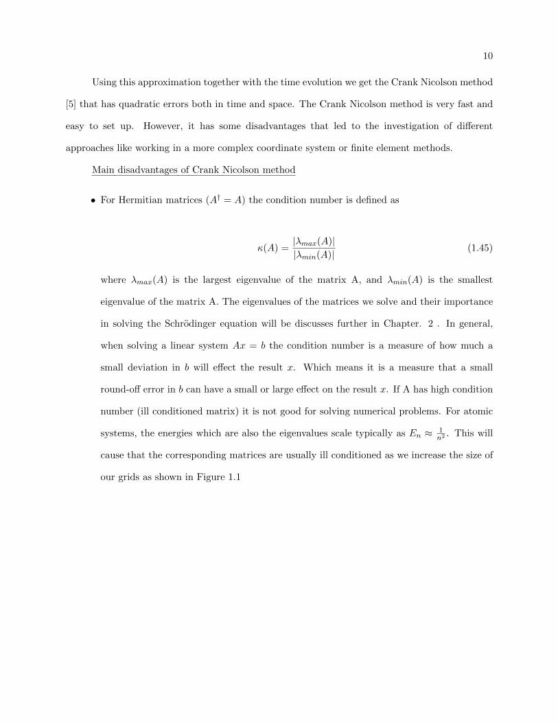
systems, the energies which are also the eigenvalues scale typically as En ≈ 1n2 . This will

cause that the corresponding matrices are usually ill conditioned as we increase the size of

our grids as shown in Figure 1.1

11

Figure 1.1: Condition number of the Hydrogen Hamiltonian in cylindrical coordinate system. The

number of grid points is equal along both radial axis and the z axis while the grid spacing is 0.1

and 0.2 respectively.

• Integrating linearly between the points with uniform grid spacing, the errors cannot get

better than O(h2) for integration without any further information on the derivative of the

wavefunction. This follows directly from the Euler–Maclaurin formula

I =

∫ xn

x0

f(x)dx = h(f0

2+ f1 + ...+ fn−1 +

fn2

) +h2

12(f′0− f

′n)− h4

720(f′′′0 − f

′′′n ) + .... (1.46)

Integration is typically used in many strong–field problems since every calculation typi-

cally involves normalization process or the determination of an expectation value, both

operations are executed by using an integral.

In this thesis we also use higher order finite difference schemes, these schemes are simply

derived by using more points so we can cancel higher order terms. For example, two steps forward

is given by

12

Ψ(t)r+2 = Ψ(t)

r + (2h)Ψ′(t)r +(2h)2

2!Ψ′′(t)r +

(2h)3

3!Ψ′′(t)r +O(h4) (1.47)

Similarly, we can have n forward or backward steps expanded in a similar manner. Then, to derive

central difference formula with fourth order accuracy we use five points and get the coefficients to

be.

Ψ′′(t)r =− 1

12Ψ(t)r−2 + 4

3Ψ(t)r−1 − 5

2Ψ(t)r + 4

3Ψ(t)r+1 − 1

12Ψ(t)r+2

h2+O(h4) (1.48)

Similarly, we can get higher order schemes for the first derivative term.

In most of the simulations presented in this thesis we use cylindrical coordinates and need

a special treatment when the radial coordinate is zero (ρ = 0). If the wavefunction derivative

at ρ = 0 would be smooth, then we could use symmetry condition such ρ(x) = ρ(−x). But

we know that the radial wavefunctions behave approximately like ≈ e−r for r > 0, leading to a

discontinuous derivative at ρ = 0. Evidently, avoiding the symmetry condition as the boundary

condition improves our results, in particular we used forward difference to solve this issue. For

example, the second derivative forward difference is given by

Ψ′′(t)r =2Ψ

(t)r − 5Ψ

(t)r+1 + 4Ψ

(t)r+2 −Ψ

(t)r+3

h2+O(h2) (1.49)

In this way we can achieve better approximation for the derivative and avoid the discontinuity. A

quick algorithm to find the coefficients to approximate derivative terms along n nodes is given in

[6].

1.2.4 Multi-dimensional systems

For a simple quantum problem in one dimension it is straight–forward to see that for k grid

points along this dimension, the wavefunction Ψ is a (k× 1) vector and the Hamiltonian is (k× k)

matrix. In general, if we have n particles and m dimensions the wavefunction will be represented

by

13

Ψ(~r1, ~r2, ..., ~rn) = ψ(1)(~r1, ~r2, ..., ~rn)⊗ ψ(2)(~r1, ~r2, ..., ~rn)⊗ ...⊗ ψ(n)(~r1, ~r2, ..., ~rn) (1.50)

where ⊗ denotes a tensor product, and the upper case index denotes a particle index . Each

function ψ(i) is represented by

ψ(i)(~r1, ~r2, ..., ~rn) = ψ(1)1 (~r1, ~r2, ..., ~rn)⊗ ψ(1)

2 (~r1, ~r2, ..., ~rn)⊗ ...⊗ ψ(1)m (~r1, ~r2, ..., ~rn) (1.51)

where the lower case number denotes the spatial dimension. For example, in Cartesian coordinate

system the lower cases are 1 = x, 2 = y, 3 = z.

Let us exemplify the notation by considering two 1D wavefunctions ψ(1)

(m×1)and ψ(2)

(n×1)with sizes

m and n respectively, in a potential V (~r1, ~r2). The joint wavefunction is Ψ(mn×1)

= ψ(1) ⊗ ψ(2).

Thus, the 1D wavefunctions are given by

ψ(1) =

ψ(1)(1)

ψ(1)(2)

.

.

.

ψ(1)(m)

, ψ(2) =

ψ(2)(1)

ψ(2)(2)

.

.

.

ψ(2)(n)

(1.52)

and the joint wavefunction is represented by

14

Ψ =

ψ(1)(1)ψ(2)

ψ(1)(2)ψ(2)

.

.

.

ψ(1)(m)ψ(2)

=

ψ(1)(1)

ψ(2)(1)

ψ(2)(2)

.

.

.

ψ(2)(n)

ψ(1)(2)

ψ(2)(1)

ψ(2)(2)

.

.

.

ψ(2)(n)

.

.

.

ψ(1)(m)

ψ(2)(1)

ψ(2)(2)

.

.

.

ψ(2)(n)

(1.53)

The Hamiltonian of this system is given by

H = P (1) ⊗ I(2) + I(1) ⊗ P (2) + V (~r1, ~r2) = −1

2

(∂

∂r1

)2

− 1

2

(∂

∂r2

)2

+ V (~r1, ~r2) (1.54)

where I(k) is the identity matrix with the size of the kth wavefunction.

To represent the system on a computer as matrices we use the finite difference methods,

discussed above. For example P (1) is given by

P (1) =

(∂

∂r1

)2

=−ψ(1)(j − 1) + 2ψ(1)(j)− ψ(1)(j + 1)

(h(1))2(1.55)

15

where h(1)is the grid spacing for ψ(1). To write it as a matrix we denote d(1) = 2(h(1))2 and u(1) =

−1(h(1))2 . The Hamiltonian H can be written as sum of 3 matrices

P (1)

(mxm)⊗ I(2)

(nxn)=

d(1)I(2) u(1)I(2) 0 . . 0 0

u(1)I(2) d(1)I(2) u(1)I(2) 0 . . 0

0 . . . . . .

. . . . . . .

. . . u(1)I(2) d(1)I(2) u(1)I(2) 0

0 . . 0 u(1)I(2) d(1)I(2) u(1)I(2)

0 0 . . 0 u(1)I(2) d(1)I(2)

(1.56)

I(1)

(mxm)⊗ P (2)

(nxn)=

P (2) 0 . . . 0 0

0 P 2x(2) 0 0 . . 0

0 . . . . . .

. . . . . . .

. . . 0 P 2x(2) 0 .

0 . . . 0 P 2x(2) 0

0 0 . . . 0 P 2x(2)

(1.57)

V (x(1), x(2)) =

V (r1(1), r2(1)) 0 0 . . . 0 0 0

0 V (r1(1), r2(2)) 0 0 . . . 0 0

0 . . . . . . . 0

. . . . . . . . .

. . . 0 V (r1(1), r2(n)) 0 . . .

. . . . 0 V (r1(2), r2(1)) 0 . .

0 . . . . 0 . 0 .

0 0 . . . . 0 . 0

0 0 0 . . . . 0 V (r1(m), r2(n))

(1.58)

Thus, the Hamiltonian will be of the form

16

H =

D UD2 0 . . 0

UD2 D UD2 0 . .

0 UD2 . . . .

. . . . UD2 0

. . 0 UD2 D UD2

0 . . 0 UD2 D

UD1 0 . . . 0

0 UD1 0 . . .

. 0 . . . .

. . . . 0 .

. . . 0 UD1 0

0 . . . 0 UD1

0 0 0

UD1 0 . . . 0

0 UD1 0 . . .

. 0 . . . .

. . . . 0 .

. . . 0 UD1 0

0 . . . 0 UD1

D UD2 0 . . 0

UD2 D UD2 0 . .

0 UD2 . . . .

. . . . UD2 0

. . 0 UD2 D UD2

0 . . 0 UD2 D

0 0 0

0 . . . 0

0 0 . . .

0 0 0 . .

(1.59)

where D = 2(h(1))2 + 2

(h(2))2 + V , UD1 = −1(h(1))2 , UD2 = −1

(h(2))2 . As seen above it consists of a main

diagonal and 4 off diagonals. In general, the number of off diagonal terms will be twice the amount

of dimensions we consider in the calculation (upper and lower for each dimension).

Using this notation we can easily see why solving the time dependent or independent

Schrodinger equation in multiple dimensions is computationally demanding. Consider a simulation

with k points along each dimension for each wave function, the size of Ψ will be (kmn × 1). For

example, lets describe a three particle system with 100 points along each dimension. The represen-

tation of the wavefunction will consist of 1009 data points. Thus, storage of this information as a

simple array of real doubles will take ∼ 8× 109 GB. Regardless of that, in this thesis we use these

methods for small enough systems as one particle with two spatial dimension and two particles

with one spatial dimension each.

The CRS format

The Hamiltonian matrices are always very sparse, to store them one uses the CRS format

(compressed row storage). In this method one stores only the non–zero values and their locations.

17

The format is using three vectors, namely

val - a vector that contains all the non zeros values

col - a vector that contains the column index of each value

row index - a vector that indicates you how many non zeros are in each row

For example, the matrix

A =

0 2 0 4 0

1 0 0 0 5

0 3 6 3 0

9 0 0 0 1

2 0 0 0 0

is stored as (using C++ indexing starting from zero)

val = [2, 4, 1, 5, 3, 6, 3, 9, 1, 2]

col = [1, 3, 0, 4, 1, 2, 3, 0, 4, 0]

row index = [0, 2, 4, 7, 9, 10]

A way to read the above is: stay on row 0 until you hit the second non value in val, then

switch to row 1 until you get to the fourth value of val and so on. When you reach the 10th value

switch to row 4 which does not exist, then you know you scanned through all the non zeros of the

matrix.

1.2.5 Orthogonalization

A necessary procedure for some of the calculations in strong-field and atomic physics is

orthogonalization. Since all the eigenvectors of Hermitian matrices are orthogonal to each other,

we can use this property to find more eigenvalues by enforcing orthogonalization as shown in

Chapter 2.2. The orthogonalization property can also be used as measure of the accurateness of

18

our calculations for the eigenstates. The methods Gram Schmidt (GS), Modified Gram Schmidt

(MGS) and Double Modified Gram Schmidt (DMGS) have been explored, having in mind that we

want to balance between minimizing the numerical error and the computational cost.

• Gram Schmidt

For a given set of vectors {v1, .., vn} the Gram-Schmidt method can be written as:

u1 = v1 (1.60)

uk = vk −k−1∑j=0

projuj (vk) (1.61)

where

proju(v) =〈v, u〉〈u, u〉

u (1.62)

If one is interested in an orthonormal set, one can normalize the set after calculation of each

uk or in the end.

Theoretically, the operation

v = v − 〈v, u〉〈u, u〉

u (1.63)

leads to othogonalizaion of v and u. However, numerically on the computer we expect a round off

error ε such that

〈v, u〉 = 〈v, u〉 − 〈v, u〉〈u, u〉

〈u, u〉 = ε (1.64)

Thus, for orthogonality of the first and the last vectors of the set, we expect:

〈u1, uk〉 =

n−1∑k=1

εk (1.65)

In general, the Gram Schmidt method is therefore not used in practice and a more common

way to orthogonalize vectors is the Modified Gram Schmidt technique.

• Modified Gram Schmidt

19

To avoid the accumulation of round off errors included in the Gram Schmidt method, a slight

modification can be done which is called the Modified Gram Schmidt (MGS) technique. To this end,

one overwrites uk each time, such that each vk is orthogonalized with respect to ui (i = 1, .., k− 1)

instead of the original vi vectors. Let the upper script denote the iteration number such that u(k−1)k

is the final version of uk, and we get:

u(1)k = vk − proju1(vk) (1.66)

u(2)k = u

(1)k − projuk−1

(u(1)k ) (1.67)

u(k−1)k = u

(k−2)k − projuk−1

(u(k−2)k ) (1.68)

This way, we orthogonalize the k-th vector with respect to all k − 1 existing ones, ui , i =

1, .., k − 1 vectors, and avoid the addition of round off errors

• Double Modified Gram Schmidt

Another common method is known as the Double Modified Gram Schmidt [2] (DMGS) which

is simply using both methods GS and MSG one after the other. This means, if one uses GS to

create an orthonormal set V , applying MSG on the set V will avoid doing the whole process on

an non-orthonormalized set. As can be seen in table 1.1, MGS can fail as well for high condition

number matrices while DMGS preforms well.

20

ρ(A) GS MSG DMSG

102 1.99 5.88E-14 4.25E-15

103 2.01 5.67E-13 3.60E-15

104 2.01 5.69E-12 3.34E-15

105 2.01 5.69E-11 3.33E-15

106 2.01 5.73E-10 3.48E-15

107 2.01 5.94E-09 3.57E-15

108 2.01 6.11E-08 3.76E-15

109 2.01 5.70E-07 3.91E-15

1010 2.02 5.81E-06 3.31E-15

Table 1.1: Comparing errors for the different orthogonalization methods for a fixed (1000× 1000)

size matrix

• Computational results

For our calculations we use MGS and not DMGS. To support that the MGS is sufficient,

both methods have been tested for several cases. A matrix condition number in Euclidean space is

defined by

ρ(A) =||σmax(A)||2||σmin(A)||2

(1.69)

where σi is called a singular value of matrix A. It is defined to be the square root of an eigenvalue of

the matrix A†A. For purpose of testing, we construct a high condition number matrix by creating

a diagonal matrix and using a unitary transformation (recall that a unitary transformation will

not change the condition number). As part of our tests, we defined diagonal matrices with values

that are linearly spaced between 1 and k−1, where k is the desired condition number of the matrix

A = Diag(1, .., k−1). For example: if k = 109 then ρ(A) = 110−9 = 109. Using randomize unitary

matrix generator we perform the unitary transformation V = BAC†, where B and C are unitary

21

matrices (B†B = I and C†C = I). All three algorithms above where performed on the columns of

V to create a subset Q ⊂ Rn , which consists of orthonormal vectors based on V . The error of the

method is represented by ||I −Q†Q||2 in the tables. If Q would be truly an orthonormal set then

||I −Q†Q||2 = 0 .

Why MGS is sufficient? As seen in table 1.1, MGS fails for high condition number

matrices when we need to orthogonalize the whole set. However, in our problems we look for at

most 50 eigenvectors out of ∼ 106 which is less than 1% of the whole set. Running several tests

on the algorithms using small (about 200) random subset of the vectors, it seemed to be sufficient

to use MGS method as shown in table 1.2. In general, the error using MGS was the same as

compared to DMSG up to 50% of the whole set, and that is definitely more than sufficient for our

kind of problems. To support the results of table 1.2, the test ran hundreds of times with a different

random subset of vectors each time and yield the same results.

ρ(A) GS MSG DMSG

102 0.129411887 2.23E-15 2.22E-15

104 0.136876775 1.53E-15 1.46E-15

106 0.171929674 1.12E-15 1.11E-15

108 0.138433878 1.79E-15 1.89E-15

1010 0.143160406 1.80E-15 1.78E-15

Table 1.2: Comparing error for the different orthogonalization methods for a fixed (1000 × 1000)size matrix and orthogonalize random 10% of the matrix vectors

Chapter 2

Imaginary Time Propagation

In this Chapter we will provide an analysis for a popular method used in numerical sim-

ulations of time–dependent Schrodinger equation called the Imaginary Time Propagation (ITP).

First, we will give an overview and motivate the method, then proceed with a more rigorous anal-

ysis. First, we will introduce iterative techniques called ”Power Methods” so that we can use them

to demonstrate how ITP works. Finally, we will provide some numerical results to compare the

method with similar techniques.

Recall from Chapter 1.2.2, the time propagation equation is given by:

(1 + i

∆t

2H

)Ψ(~r, t+ ∆t) =

(1− i∆t

2H

)Ψ(~r, t) . (2.1)

The Imaginary Time Propagation method simply calls to use ∆t = −iτ , τ ∈ R in the time

propagation Equation (2.1) and then to normalize the wave function Ψ(~r, t + ∆t) = Ψ(~r,t+∆t)||Ψ(~r,t+∆t)||

for each time step. Equation (2.1) is a discretized version of the time propagation operator as

demonstrated in Chapter 1.2.1. To motivate the Imaginary Time Propagation method we will first

show why it works using continuous quantum operators.

2.1 The general idea

Recall that for the time-independent potential, we can separate the Schrodinger equation and

the wavefunction into time dependent and time independent parts:

23

time dependent: Eφ = i~∂φ

∂t→ φ = e−iEt (2.2)

time independent: Hψi = Eiψi (2.3)

where the total wavefunction is separated into a product of independent variable functions

Ψ(x, t) = ψ(x)φ(t) (2.4)

The time independent solutions ψ(x) are called stationary states since they do not change

over time. There are two types of stationary states, bound states and continuum states. Bound

states are bounded by the attractive Coulomb potential from the nucleus (the energy of the electron

in this state is less than the potential).

In general, for large distances an attractive Coulomb potential scales inversely over distance

such that

Vcoulomb(r) ≈ −1

r(2.5)

Note that the distance r is always positive, therefore the potential is bounded by zero as r goes

to infinity, which means all bound states have energy less than zero. Continuum states are not

bounded by the attractive potential and have positive energy. The least energetic bound state we

denote by ψ0 and call it the ground state. It solves the TISE (2.3) such that

Hψ0 = E0ψ0 . (2.6)

Hence, E0 is the most negative energy and mathematically the most negative eigenvalue. Any ex-

cited states (bound states with higher energy than the ground state) are also obeying the eigenvalue-

eigenvector Equation (2.7). We denote an eigenpair of a bound state ψi and energy Ei by (ψi, Ei)

Hψi = Eψi (2.7)

24

Any quantum state can be expressed as a linear combination of its stationary states and their

associated time dependent parts

Ψ(~r,∆t) =

∞∑i=0

ciψie−iEi∆t +

∫ ∞0

ciψie−iEi∆tdEi , (2.8)

where ci is a time dependent coefficient and φi is the time dependent wavefunction from

equation (1.7). If we use negative imaginary time ∆t = −iτ , then Equation (2.8) becomes

Ψ(~r,∆t = −iτ) =

∞∑i=0

ψie−Eiτ +

∫ ∞0

ciψie−EiτdEi (2.9)

Since all continuum states have positive energy, for large τ their contributions will vanish.

As for the bound states, the energies are negative and the ground state energy is the most negative

of them. Then, for large τ only the ground state contribution with the largest exponential term

will dominate

limτ→∞

Ψ(~r,∆t = −iτ) ≈ limτ→∞

ψ0e−E0τ . (2.10)

Once this state is normalized we get the ground state

limτ→∞

Ψ(~r,∆t = −iτ)

||Ψ(~r,∆t = −iτ)||= ψ0 (2.11)

The method will converge to the most negative energy state. On the computer however we

are not using e−Ei∆t but the approximation given by Equation (2.1). To provide analysis how the

wave function evolves using imaginary time propagation on the computer we first introduce simpler

iterative techniques called Power Methods.

2.2 Iterative Methods

2.2.1 Power Iteration

One of the most fundamental iterative techniques to find the largest eigenvalue of a square

matrix is the power method, in which the matrix is applied multiple times on a vector. By normal-

25

izing the vector, the method converges to the eigenvector with the largest eigenvalue. First, recall

that for a square (n× n) matrix A an eigenvalue λ and an eigenvector v are given by

Av = λv (2.12)

Lets consider a (n × n) full rank matrix A with eigenpairs (λi, vi), i = 1, ..., n. Then any vector

x ∈ Rn can be expressed as

x =

n∑i=1

civi . (2.13)

Multiplying the matrix several times on the vector x, we get

Akx =n∑i=1

ciλki vi . (2.14)

In order to guarantee that the power method will converge to an unique eigenvector, we need

to assume that there exist a eigenvalue that is larger than all the other eigenvalues in magnitude

|λ1| > |λ2| ≥ |λ3| ≥ ... ≥ |λn| .

Using this assumption we can factor out the largest eigenvalue and see that for large enough k all

the rationals will converge to zero

Akx = λk1

[c1v1 + c2

(λ2

λ1

)kv2 + ..+ cn

(λnλ1

)kvn

]≈ c1λ

k1v1 . (2.15)

By normalizing Akx we get the normalized eigenvector corresponding to the largest eigenvalue:

v1 ≈Akx

|Akx|(2.16)

To get the eigenvalue we use Rayleigh quotient

λ1 =〈v1, Av1〉〈v1, v1〉

(2.17)

26Algorithm 1 Power Method

1: procedure PowerMethod(A,x)2: for k=1,2,... do3: x← Ax4: x← x/||x||5: end

This method can be implemented on the computer via a general algorithm (see algorithm 1).

Convergence:

To determine how fast the method will converge, we identify the slowest decaying term of the series

from Equation (2.15) as |λ2||λ1| . Clearly, the closer to zero the term is, the faster the method will

converge. To define a convergence rate, consider the sequence x(1), x(2), x(3), ..: We say the sequence

converges to a value x in order p, if there exist a constant C > 0 such that

limn→∞

|x(n+1) − x||x(n) − x|p

= C , (2.18)

where C is called the proportionality constant. For p = 1, the method in linearly convergent, if

C ∈ (0, 1), and C is called the rate of convergence. To analyze convergence rates for the power

method, consider the sequence x(1), x(2), x(3), ... where

x(n+1) =Ax(n)

||Ax(n)||. (2.19)

Using Equation (2.15) we get

|x(n+1) − v1| = O

(∣∣∣∣λ2

λ1

∣∣∣∣k) , (2.20)

where O(x) = Cx | C ∈ R . Applying Equation (2.20) in the definition of convergences (2.18) we

get

limn→∞

|x(n+1) − v1||x(n) − v1|

=

∣∣∣∣λ2

λ1

∣∣∣∣ (2.21)

27

This tells us that the power method will converge linearly (p = 1) to v1 with a rate of convergence∣∣λ2λ1

∣∣Possible issues: If the vector x is orthogonal to v1 then c1 = 0 and the method will not

converge to v1 but to v2. In general, choosing a “good” initial guess will always help the method

the converge faster.

Applying the power method to the physical system: The power method can be applied to

the TISE describing an atom or a molecule, since |E0| > |E1| > |E2|... are eigenvalues of the

Hamiltonian. However, since continuum states have energy in magnitude, a slight modification

should be introduced to make the method converge to a desired eigenvalue. This method is called

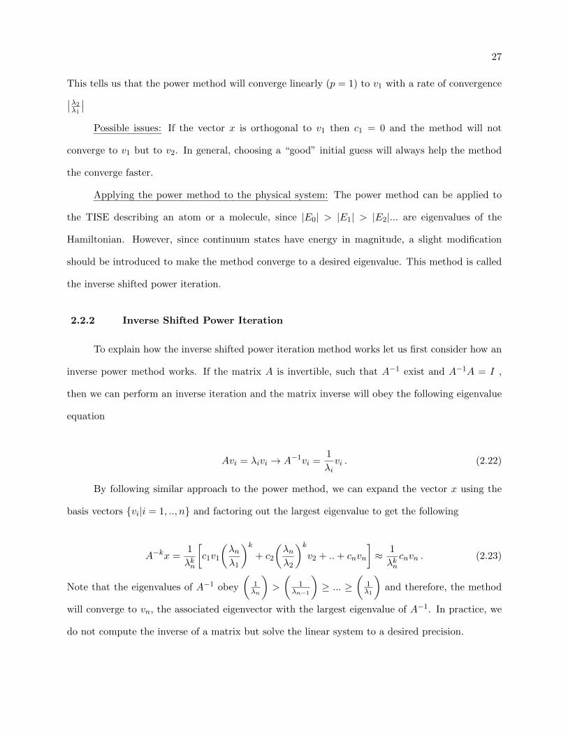
the inverse shifted power iteration.

2.2.2 Inverse Shifted Power Iteration

To explain how the inverse shifted power iteration method works let us first consider how an

inverse power method works. If the matrix A is invertible, such that A−1 exist and A−1A = I ,

then we can perform an inverse iteration and the matrix inverse will obey the following eigenvalue

equation

Avi = λivi → A−1vi =1

λivi . (2.22)

By following similar approach to the power method, we can expand the vector x using the

basis vectors {vi|i = 1, .., n} and factoring out the largest eigenvalue to get the following

A−kx =1

λkn

[c1v1

(λnλ1

)k+ c2

(λnλ2

)kv2 + ..+ cnvn

]≈ 1

λkncnvn . (2.23)

Note that the eigenvalues of A−1 obey

(1λn

)>

(1

λn−1

)≥ ... ≥

(1λ1

)and therefore, the method

will converge to vn, the associated eigenvector with the largest eigenvalue of A−1. In practice, we

do not compute the inverse of a matrix but solve the linear system to a desired precision.

28

If we present a shift α to the matrix A such that

(A− Iα)vi = Avi − Iαvi = λivi − Iαvi = (λi − Iα)vi (2.24)

then for power iteration the method will converge to the eigenvalue farthest away from α

which is not really useful. On the other hand, performing the shift with the inverse power iteration

will converge to the eigenvalue closest to the shift, which provide a powerful way to look selectively

for a specific eigenvalue.

Similarly to the power method, as shown in [11] the convergence of the inverse power method

follows a linear rate of

limn→∞

|x(n+1) − v1||x(n) − v1|

=

∣∣∣∣ λn − αλn−1 − α

∣∣∣∣ , (2.25)

where λn is the closest eigenvalue to α and λn−1 is the second closest.

Using the literature values for the energies, we apply the inverse power iteration to find

specific bound states. If literature values are not available, we exploit the fact that the only negative

eigenvalues will be bound states. If we attempt to converge to a large negative number, the method

will converge to the closest negative number next to it. Thus, as long as we choose a large enough

negative energy, the method will converge to the ground state.

Algorithm 2 Inverse Power Method

1: procedure InversePowerMethod(A,x,α)2: for k=1,2,... do3: x← (A− Iα)−1x4: x← x/||x||5: end

2.2.3 Rayleigh Quotient Iteration

As can be seen from Equation (2.25), the choice of α will influence the rate of convergence.

An adaptive approach for choosing a shift is usually preferred, since in every iteration we can make

use of the new knowledge about the ideal value. An interesting special case is to choose the Rayleigh

Quotient

29

λ(k) =〈v(k), Av(k)〉〈v(k).v(k)〉

(2.26)

as the shift for each iteration, which gives cubical convergence when we get close enough to the

eigenvalue [14].

2.3 Analysis of Imaginary Time Propagation

The Imaginary Time Propagation (ITP) is an iterative algorithm (algorithm 3), as the power

methods, however it is a bit more complex. To get an intuition, we can look at a single iteration

using the analysis of the power method. Recall the system we are solving on the computer is set as

(1 + i

∆t

2H

)Ψ(~r, t+ ∆t) =

(1− i∆t

2H

)Ψ(~r, t) . (2.27)

Using negative imaginary time we get

(1 +

τ

2H

)Ψ(~r, t− iτ) =

(1− τ

2H

)Ψ(~r, t) . (2.28)

To simplify the notation, let x(~r, t) be the right hand side such that

x(~r, t) =

(1− τ

2H

)Ψ(~r, t) =

∞∑m=0

cm(1− τ

2λm)ψm . (2.29)

Then, one can interpret x(~r, t) as a somewhat amplified vector of Ψ(~r, t) by a single shifted power

iteration. Using the power method convergence analysis the right hand side vector x will converge

to ψ with the largest energy L1 = max(1 − τ2λ) with a rate of L2

L1, where L2 is corresponding to

the second largest value of (1 − τ2λ). In general, the method will converge to the most negative

eigenvalue. Since τ is small, τ2λ� 1 and we expect the convergence to be slow.

On the other hand, if we consider the left hand side for a fixed x(~r, t) we get

(1 +

τ

2H

)Ψ(~r, t− iτ) = x(~r, t) , (2.30)

30

which will converge to ψ with the smallest energy S1 = min(1 + τ2λ) with a rate of S1

S2where S2

is corresponding to the second smallest value of (1 + τ2λ). In general, since τ is small we have

τE0 � 1, and hence the ratio L2L1

is close to 1, which leads to slow convergence.

Possible issues: If τ is chosen to be too large, it will cause the eigenvalue of τ2 H to be smaller

than -1 and then the method will not converge to the ground state.

To find excited states the method requires to orthogonalize each iteration with respect to

lower states that are already obtained. Therefore, since E2i+1 < E2

i for bound states, convergence is

guaranteed but not necessarily fast. In fact, the demand for high accuracy with orthogonalization

using the Gram Schmidt method will not allow convergence after several states.

Disadvantage of Imaginary time propagation:

• No control over the state one will find. The only parameter one can change is τ , which

cannot be too large since it will cause stability issues for the Crank Nicholson method.

Also, it is hard to predict exactly what τ one needs to scale H so that the method will

converge to the (-1) shift created by the time propagation equation

(τ2 H − (−1)

).

• Converges to one state at the time. Unlike simultaneous iteration techniques (see Chapter

3), the ITP method converges to one state at the time

• Slow convergence rates and numerical errors prevent to find many states with higher energy.

So why is it so common?

• The ITP is a working method that can be implemented with a minor change in the actual

time propagation (Equation (2.1)).

• In combination with the Split Operator method the size of the system can be reduced. For

example, a system of a size (n2 × n2) can be reduced to n smaller (n × n) systems which

are faster to solve.

31Algorithm 3 Imaginary Time Propagation

1: procedure ITP(Ψ,H,∆t)

2: Eold ← 〈Ψ,HΨ〉〈Ψ.Ψ〉

3: while error ≤ 10−16 do

4: b←(

1− i∆t2 H

)Ψ(~r, t)

5: A←(

1 + i∆t2 H

)Ψ(~r, t)

6: Psi← A−1b7: E ← 〈Ψ,HΨ〉

〈Ψ.Ψ〉8: error ← abs(E−EoldE )9: Eold ← E

10: end

2.4 Comparison of results

To analyze the performance, we used an existing code for the ITP method to obtain excited

states and compared the results with those of the Inverse Shifted Power method. In both cases

we used the modified Gram Schmidt for orthogonalization. As a test case we used a 1D Helium

system (two electrons with one spatial dimension each), then the Hamiltonian is

H = P (1)⊗I(2) +I(1)⊗P (2) +V (~x1, ~x2) = −1

2

(∂

∂~x1

)2

− 1

2

(∂

∂~x2

)2

− 1

|~x1|− 1

|~x2|+

1

|~x1 − ~x2|(2.31)

where P (1) ⊗ I(2) is the kinetic energy of the first electron, I(1) ⊗ P (2) is the kinetic energy of the

second electron , and V (~x1, ~x2) is the electron-nucleus and electron-electron interactions.

For the test we used the same machine, a 80 × 80 atomic units grid with 0.1 a.u. grid

spacing in each dimension. The bound states are denoted by {Ei , i = 0, 1, 2, ..} such that E0 is the

ground state and has the most negative energy (|E0| > |E1| > ..) . For the test, we used a fixed

shift for the Inverse Shifted Power Method (ISPM). Usually, we could change the shift to accelerate

convergence, but for this comparison we kept it fixed. Both methods converged correctly to the

first five bound states with energies given in atomic units (a.u) as shown below

32

E0(a.u) E1(a.u) E2(a.u) E3(a.u) E4(a.u)

−2.238 −1.816 −1.705 −1.644 −1.629

(2.32)

However, the time used in the ITP was significantly longer as can be seen from data shown

in table (2.1). While it takes a full hour and close to 3000 iterations for the ITP to converge to the

ground state, in the Inverse Shifted Power Method (ISPM) the same result is achieved in 6 seconds

and only 5 iterations. In general, the ITP is indeed incomparably slower.

ITP(hr) steps ISPM(min) steps

E0 1.01 2864 0.09 5

E1 6.68 26883 3.23 155

E2 10.89 23104 2.93 414

E3 9.51 45232 5.69 314

E4 16.92 19676 17.85 168

Table 2.1: Comparison of time and number of iterations (steps) taken for the Imaginary Time

Propagation (ITP) and the Inverse Shifted Power Method.

As can be seen from table (2.1), for all 5 states together it took ISPM less than half of the

time that the ITP needs to obtain a single state. However, even the convergence rate of the ISPM

method decreases significantly after a few states. This is due to dense eigenvalues and orthogo-

nalization errors that can be avoided using an adaptive shift in the ISPM or via a whole different

method such as the Arnoldi iteration (Chapter 3).

As mentioned, both methods are iterative power methods and their rate of convergence can

be predicted. To confirm the proposed analysis discussed earlier in the Chapter, we have analyzed

the error for each iteration. For the Imaginary Time Propagation, the theoretical convergence rate

for the ground state of the left hand side is given by

33

CITP LHS =

∣∣∣∣S1

S2

∣∣∣∣ ≈ 0.9768 , (2.33)

while for the right hand side it is given by

CITP RHS =

∣∣∣∣L2

L1

∣∣∣∣ ≈ 0.9810 . (2.34)

Both values are very close to the numerical result CITPNu = 0.987. Overall, as shown in

table (2.2), the predictions for the convergence rate in the ITP are not far for the numerical values.

For this given test, the ISPM was far off theory and, in particular, faster than predicted for the

lower states. This happens due to the exact shift we picked (using the literature value), the method

converges within a few iterations, which makes it difficult to get accurate values of the rate of

convergence constant. Consider CISPM , which is the linear rate of convergence constant for the

ground state using ISPM. By picking the shift to be very close to E0, the ratio

CISPM|E0 − α||E1 − α|

(2.35)

is almost zero and hence we converge within a few steps. For the higher states the numerator

does not converge to zero and the rate of convergence, given by C(i)ISPM = |Ei−α|

|Ei+1−α| , is getting more

accurate.

To obtain states with higher energy using ISPM, we need to update the shift we have chosen

to obtain good convergence rates. As can be seen from Figure 2.1, these states are closer to each

other in energy and an accurate or adapted shift is needed to converge fast.

34

Figure 2.1: Energy of stationary states of 1D helium atom ordered by the magnitude of their energy.

In this plot we present the smallest 2000 energies.

state ITPEx ITPTh % Error ISPMSm ISPMLt % Error

E0 0.994 0.976 1.723 N/A 0.0013

E1 0.998 0.993 0.423 0.692 0.790 -14.295

E2 0.999 0.996 0.250 0.875 0.897 -2.528

E3 0.998 0.999 -0.079 0.961 0.975 -1.529

E4 0.999 0.997 0.154 0.919 0.929 -1.037

Table 2.2: Linear rate of convergence constants for the Imaginary Time Propagation (ITP) and

the Inverse Shifted Power Method (ISPM) for the 1D helium test case. Subscript (Sm) denotes

simulation value and subscript (Lt) denotes literature value, the error shown is the given relative

error between them.

35

2.5 Summary

The Imaginary time propagation is an iterative method to find eigenstates and has no par-

ticular advantage, numerically or quantum mechanically. Once we an use imaginary time step the

time evolution operator is no longer unitary and therefore not representing a real physical opera-

tor anymore. Converting the ITP method into an inverse shifted power method can be done by

changing the existing ”1” on the left-hand side of the ITP into a variable (which will denote as the

shift), picking ∆t = 2 and using the existing wave function as the right-hand side.

(1 +∆tH

2)→ (α+

2H

2)→ (H − (−α)) . (2.36)

This small modification will increase drastically the convergence rate for few eigenstates in com-

parison to the ITP.

Chapter 3

Application of Arnoldi algorithm

In Chapter 2 the Imaginary Time Propagation method was analyzed and shown to be slow

and limited in obtaining more than few bound states. The ITP was compared to the Inverse

Shifted Power Method, a known technique but with the limitation of finding one eigenvalue at a

time. In this Chapter we will introduce subspace iteration techniques and, in particular, discuss

the application of the Implicitly Restarted Arnoldi method [12] for problems in AMO physics.

3.1 Overview

A common way to find more than one eigenvalue, while using iterative methods, is to ap-

ply deflation techniques. One of them was introduced in Chapter 2, namely orthogonalization

with respect to previously obtained vectors. Another common approach is to work with a block

format (several vectors at the time), which also called Subspace Iteration. As will be shown

in algorithm 4 , for a matrix A with dimension (n × n) and a given set of non-parallel vectors

V = {[v1, v2, ...] | vi ∈ Rn , i = 1, 2, ..}, we perform a matrix-matrix multiplication (every column

vector in the matrix V gets multiplied by the matrix A), and then we orthogonalize the new matrix

(every column vector gets orthogonalized to the previous vectors in the set), typically, with the use

of the QR algorithm [7].

37Algorithm 4 Subspace Iteration for Hermitian positive definite matrices

procedure Subspace Iteration(A,V)

for k=1,2,... do

V ← AV

V ← orthonormalize(V )

end

Finding an initial subspace that will guarantee fast convergences rate for the subspace iter-

ation to preform well is not an easy task. One common subspace is the Krylov subspace, for a

matrix A with dimension (n × 1) it is the natural subspace produced by the power method and

denoted by

Kk(A, v) = span{v,Av,A2v, .., Ak−1v} , (3.1)

where k is the dimension of the space such that k ≤ n.

By performing a Gram-Schmidt process on the basis vector of Kk, a general Arnoldi basis is

created. The Arnoldi basis vectors are denoted by qi

qi =yi||yi||

(3.2)

with

yi = Aiv −i∑

j=1

qjq†jA

iv . (3.3)

The above is the normal Gram Schmidt process, which is however computationally expensive.

A more economical way to compute qi+1 is given by defining

ri = Aiqi −i∑

j=1

qjq†jA

iqj , (3.4)

where qi+1 is given by

38

qi+1 =ri||ri||

(3.5)

By construction (seen from Equations (3.4) and (3.5)) qi+1 is orthogonal to all previous Arnoldi

vectors. Then we define

hij = q†iAqj (3.6)

which can be collected to a matrix form, and we can introduce the Arnoldi relation:

AQk = QkHk + [0, ..., 0, qk+1hk+1,k] , (3.7)

where Qk = [q1, ..., qk], Hk is a (k × k) matrix with coefficients given by Equation (3.6), and the

second term on the right hand side contains k − 1 zeros.

The algorithm stops when hk+1,k = 0 which implies we form an invariant subspace of A,

AQk = QkHk . (3.8)

Since Qk is a unitary matrix, the eigenvalues of Hk are the eigenvalues of A as well and the

Ritz vectors Qkvi are the eigenvectors of A,

Hnvi = λivi → A(Qnvi) = λi(Qnvi) . (3.9)

The Arnoldi relation (3.7) gives us a computationally cheap estimate of the eigenvalues and

eigenvectors since Hn consists of zeros below the first diagonal (upper Hessenberg matrix). Efficient

algorithms such as the QR algorithm can be implemented to construct it. In practice, as n gets

larger, every step of the computation to obtain the next qi gets more expensive. However, one

can exploit the fact that extremal eigenvalues converge quickly and deflate (keep them unchanged)

them as soon as they converge within a certain error range. To improve performance, the algorithm

is performed with a target of a small subspace of size m ≤ n. Once the subspace m is reached, the

algorithm is restarted with the new and better approximation.

39

The implicitly restarted Arnoldi method is a general high–end method for computing

eigenvalues and eigenvectors and can be optimized for different cases and constraints as needed. A

common one is the Lanczos method, in which case the matrix A is Hermitian. Below we apply the

method to a problem in cylindrical coordinates and the Hamiltonian is therefor not symmetric. We

will test the performance of the implicitly restarted Arnoldi method for this set of problems and

compare it to those of previous methods.

3.2 Hydrogen atom

We first consider the simplest atom, i.e. the hydrogen atom which have only a single electron

and a single proton in the nucleus. The Hamiltonian is given by

H = −1

2∇2 − 1

|~r|(3.10)

and the TISE has known analytical solutions. Thus, we can actually check our numerical methods

by comparing the results to these analytical solutions. All the simulations were performed using

cylindrical coordinates, where ρ denotes the radial distance and z denotes the longitudinal axis.

We classify the solutions with three quantum number (n, l,m): The principal quantum number

n, n = 1, 2, 3.., the angular quantum number l is bounded by n, so that l = 0, 1, 2, .., n − 1, and

the magnetic quantum number m is an integer between −l and l. However, in our applications we

neglect φ (the polar axis), since most processes in AMO physics start with a fixed initial ground

state and linear polarization of light fields (∆t = 0). Since all wavefunctions are normalized to 1

and decay exponentially, we plot our solutions on a base ten log scale.

In Figure 3.1 we present some of the lowest eigenstates of hydrogen atom obtained using the

Arnoldi method with a second order difference scheme. Each bound state has n− l−1 radial nodes,

(zeros along a fixed half circle), and l angular nodes (zeros along radial lines). The energy of the

states was computed and compared with the exact analytical results in table 3.1.

40

Figure 3.1: First four bound states of hydrogen atom using second order finite difference scheme

with (0.1,0.2) a.u. grid spacing and (600,600) a.u. grid along ρ and z axis respectively. Up-left: 1s

, up-right: 2s , down-left: 2p , down-right: 3s.

Good agreement (within two digits of accuracy) is found for a grid spacing with ∆ρ = 0.1

a.u. and ∆z = 0.2 a.u. . We were able to reproduce the first thirty states on a (200 × 400) a.u.

grid with (0.1,0.2) grid spacing along ρ and z, respectively. Overall, the energies remained accurate

for higher excited states as well. Indeed, for higher excited states, the accuracy even gets better.

Since the wavefunction increases in size for the excited states, we may consider that the singularity

at the origin is the largest source of error in our calculations.

41

state energy calculated exact energy ∗relative error

1s -0.49443 -0.5 1.114

2s -0.12438 -0.125 0.49672

2p -0.12513 -0.125 -0.10006

3s -0.05538 -0.055555556 0.31595

3d -0.055576 -0.055555556 -0.036649

3p -0.055607 -0.055555556 -0.092836

4d -0.031262 -0.03125 -0.038355

4s -0.031178 -0.03125 0.23091

4p -0.031275 -0.03125 -0.079697

4f -0.031255 -0.03125 -0.016234

∗ relative error is measured by 100× xcalculated−xexactxexact

Table 3.1: Comparison of the energy of the first 10 bound states of Hydrogen using a (200×400)grid

with (0.1,0.2) grid spacing for ρ and z, respectively.

3.2.1 Scaling

Since we are interested in obtaining high excited bound states, it is important to study how

the numerical method scales. To this end, we ran several simulations using second order finite

difference method with different grid sizes and obtained the time to find the first ten bound states

as we increase the grid size. The grid size is given by the number of points along the radial axis

multiplied by the number of points along the longitudinal axis. For example, for a grid size of

(200,400) a.u. with grid spacing of (0.1,0.2) a.u. respectively for ρ and z, the total number of

points will be 4× 106 points.

42

Figure 3.2: Runtime to find first 10 eigenstates of Hydrogen with respect to the grid size.

As can be seen from the results in Figure 3.2, for the sizes of grids considered here (bounded by

the sizes of grids we perform simulations of the TDSE) the scaling is approximately linear, unlike

for the ITP that has a sharp exponential growth when the number of points increases.

In addition for a solver to be scalable with the grid size, we also want it to be scalable with

the number of eigenstates obtained. To this end, we used the Arnoldi solver for a fixed grid size

of (1000× 1000) a.u with (0.2,0.4) grid spacing respectively for ρ and z. In each ran we calculated

one more eigenvalue than in the previous run.

43

Figure 3.3: Runtime of the Arnoldi algorithm to find n stationary states of hydrogen atom on a

fixed (200× 400) a.u. grid with (0.2,0.4) a.u. grid spacing along ρ and z axis, respectively.

As shown in Figure 3.3 the run time grows approximately linearly as a function of the number of

eigenvalues obtained. With a basic curve fitting technique we can estimate how long it may take

to find even larger set of states. In contrast, using the ITP method, after few eigenstates the run

time grew very large.

3.2.2 Higher order finite difference methods

While second order finite difference method gives good results for the energies, we have

also investigated if even better results can be obtained with higher order finite difference schemes.

In Table 3.2 we compare the relative error of the energy of the first 10 bound states obtained by

using second, fourth and sixth order finite difference on a (200× 200) a.u. grid with (0.1, 0.2) a.u.

grid spacing respectively along the ρ and z axis.

44

state 2nd order 4th order 6th order

1s 1.114 1.251 1.2913

2s 0.49672 0.62822 0.6494

2p -0.10006 -0.0017836 -0.0010461

3s 0.31595 0.41941 0.43371

3d -0.036649 -6.0728e-05 -1.8737e-07

3p -0.092836 -0.0014742 -0.00082758

4d -0.038355 -6.9522e-05 -2.254e-07

4s 0.23091 0.31479 0.32557

4p -0.079697 -0.0011878 -0.00065495

4f -0.016234 -1.0475e-05 -1.8173e-08

∗ relative error is measured by 100× xcalculated−xexactxexact

Table 3.2: Comparison of relative error for energy of the first 10 bound states of Hydrogen obtained

using second, fourth and sixth finite difference schemes on a (200 × 400) grid with (0.1,0.2) grid

spacing for ρ and z, respectively.

As can be seen from Table 3.2, the second order scheme provides better results for low

energetic states. Evidently, these states are smaller by radius, which may indicate that the second

order scheme perform better closer to the origin. To test our expectation, we can use the state

(n,l,m)=(7,4,0) and compare the wavefunction using second and fourth order schemes.

45

(a) (b)

Figure 3.4: (n,l,m)=(7,4,0) state of hydrogen atom using (a) second order finite difference and (b)

using fourth order finite difference schemes

The comparison in Fig shows that the fourth scheme is not preforming as well close to the

saddle points, where the radial nodes and angular nodes meet. To analyze it further, we integrate

along the two radial nodes numerically and observe that the error with respect to the analytical

result is larger for the fourth order scheme along the node at 18 a.u. and the error is larger for

the second order scheme along the node at 36 a.u.. Since in the derivation of the finite difference

schemes we cancel higher order derivative terms, we might have d2ψd~r2 � d4ψ

d~r4 � d6ψd~r6 near the

singularity and then the error terms for the lower finite difference scheme will actually smaller.

The behavior observed in our numerical results may occur since finite difference schemes perform

well for polynomials. The wave function can be approximated as a polynomial far from the origin,

while close to the origin this approximation fails.

46

Figure 3.5: The analytical solution on the left compared with the numerical solution on the right

for 5s state of Hydrogen using second order finite difference method

In order to further analyze in view of potential applications, we also integrated along

angular nodes and fixed z bands (integrate all z values for a range of ρ). As can be seen from the

comparison in Table 3.3, the second order scheme performs over all better for the first two states

while the fourth and sixth order methods provide comparable results for higher excited states in

the table. Evidently, as higher excited the state is, the improvement of the sixth order becomes

more and more interesting. However, in practice we need to compromise between accuracy of the

lower states, computation times and the accuracy in the higher excited states. The fourth order

schemes appear to be a good choice and we used it for the single active electron calculations below.

47

2nd 4th 6th nlm

energy 1.114 1.2913 1.251 100

z= [-1.7 , 1.9] -1.6256 -2.3456 -2.2678 100

energy 0.49672 0.6494 0.62822 200

z= [-1.7 , 1.9] 0.59909 0.76193 0.73731 200

ρ = 2 0.59389 1.4803 1.3056 200

energy -0.10006 -0.001046 -0.0017836 211

z= [-1.7 , 1.9] -0.34966 -0.0029277 0.0050262 211

θ = 90◦ 0.27057 0.00041069 0.0037945 211

energy 0.31595 0.43371 0.41941 300

z= [-1.7 , 1.9] 3.1381 0.48468 0.50049 300

ρ = 7.10 49.6249 14.77 13.8016 300

energy -0.092836 -0.00082758 0.0014742 310

z= [-1.7 , 1.9] -0.31792 -0.0021761 -0.0039479 310

ρ = 6 1.3558 0.0060593 0.010974 310

θ = 90◦ -0.016009 0.00012216 0.00089391 310

energy -0.036649 -1.8737E-07 -6.0728E-05 320

z= [-1.7 , 1.9] -2.4043 0.035096 0.0045935 320

θ = 54.74◦ 1.8044 -0.0041971 -0.00062491 320

Table 3.3: Comparison of numerical results for first 6 states of Hydrogen using 2nd, 4th and 6th

order finite difference schemes. The values in the table represent relative error in percentage of the

calculated energy, and results of integration along fixed radii, fixed theta and fixed z bands.

48

3.3 Single active electron problems

3.3.1 Introduction

Solving the TDSE with two or more particles is extremely difficult task even on modern

supercomputers. A popular approach is called the single–active–electron (SAE) model, this model

treats all particles but one to be frozen. If one can obtain the potential created by the other

particles in the system, one can solve the TDSE for only one electron. To motivate this approach,

first consider the Born–Oppenheimer approximation. It simply says we can treat the nuclei to

be stationary in time since on the time scale of electron dynamics that positions barely change.

Second, in most interaction of matter with ultrafast laser pulse only few electrons are involved. For

some processes (like high harmonic generation) typically only one electron becomes active and the

SAE model will be the natural choice for numerical simulations. There are several about how to

create SAE potentials, in this thesis we will use a modified optimized effective potential scheme

developed in the ultrafast AMO Theory group at Boulder [13]. A single active electron potential

using the Kohn–Sham density functional formulation [1] can be represented as

Vσ(r) = −∑α

Zα|Rα − r|

+

∫ρ(r′)

|r − r′|dr′ + Vxcσ(r) (3.11)

where σ is the spin polarization and each α represents a nuclei with charge Zα at a distance Rα.

The total electron density ρ(r) is given by

ρ(r) =∑σ

Nσ∑i=1

|φiσ(r)|2 (3.12)

where φiσ is the normalized wavefunction of the ith atomic orbital with σ spin polarization. The

exchange–correlation potential is given by

Vxcσ(r) =δExc[ρ↑, ρ↓]

δρσ(r)(3.13)

and Exc[ρ↑, ρ↓] is the exchange correlation functional. Once the exchange correlation potential is

49

chosen, we can solve (3.11) and obtain the SAE potential. In [13] several approaches are being

explored, in this thesis we will use SAE potentials based on the KLI-SIC (were KLI stands for

Krieger, Li, Iafrate and SIC stands for self–interaction correction) results fitted1 into the analytical

function [9], given by

VSAE(~r) = − C|~r|− Zce

−C0|~r|

|~r|+∑i=1

aie−bi|~r| (3.14)

where Zc, c0, ai, bi | i = 1, 2, 3 are constants.

Then, we use the Arnoldi algorithm with various finite difference schemes to obtain the

resulting atomic orbitals. To test our results, we can use the experimental ionization energies

and match their energies with the excited states. Also, while we will not use very small grid

spacing for simulations involving time propagation, we can use small grid spacing to find the best

approximation achieved by the SAE potential.

3.3.2 Results

3.3.2.1 Argon

The first single active electron potential we considered is for the valence electron (ground

state: 3p orbital; (3,1,0) configuration) in Argon. We have chosen Argon since many literature

values are available for comparison. First, we studied the convergence of our results with respect

to the grid spacing. To this end, we used ∆ρ = ∆z and reduced the step size from ∆ρ = ∆z = 0.1

a.u. to ∆ρ = ∆z = 0.01 a.u..

1 Fitting coefficients produced by Ran Reiff, ultrafast AMO group, JILA

50

Figure 3.6: Relative error of the numerically obtained energy of the first three bound states of

Argon as compared to the literature value as a function of grid spacing dρ = dz.

The results in Figure 3.6 show that the relative error of the energy of the first three bound

states (with respect to the literature value) decreases as the grid spacing gets smaller. Note that

the error likely will not approach zero, since the corresponding energy from the DFT calculation

does not agree with the literature value as well. For our further studies, we chose to use the grid

spacing as dρ = dz = 0.04 a.u., for which the energy for the first valence states is within one

percent of the DFT value. To make sure that our previous conclusion concerning the use of fourth

order finite difference scheme does apply to the SAE case as well, we have also performed the same

analysis using second order scheme and indeed observe a larger error in energy (three percent of

DFT value).

51

Figure 3.7: Argon orbitals using grid spacing 0.04 for both ρ and z. Left: 3p, right: 4s.

3.3.2.2 Other atoms

To further test the quality of our results, we used SAE potentials for multiple atoms and

compared the numerical results obtained using the Arnoldi method with the DFT results and the

ITP solutions. To be consistent, all Arnoldi simulations where performed using a (64 × 128) a.u.

grid with 0.04 a.u. grid spacing for both ρ and z. Note that the ITP solutions are not obtained

with the same grid spacing, but they represent the best value that was achieved.

52

Species State DFT literature ITP Arnoldi DFT/literature Arnoldi/DFT ITP/DFT

He 1s -0.918 -0.904 -0.929 -0.918 -1.60% 0.02% -1.20%

Li+ 1s -2.793 -2.780 -2.843 -2.792 -0.47% 0.04% -1.80%

Li- 2s -0.015 -0.023 -0.013 -0.012 33.95% 19.03% 13.33%

Be 2s -0.308 -0.343 -0.312 -0.306 10.04% 0.82% -1.22%

F 2p -0.709 -0.640 -0.732 -0.711 -10.80% -0.24% -3.18%

Ne+ 2p -1.577 -1.505 -1.622 -1.590 -4.75% -0.83% -2.86%

F- 2p -0.160 -0.125 -0.178 -0.160 -28.27% 0.06% -11.06%

Ne 2p -0.807 -0.793 -0.844 -0.814 -1.84% -0.86% -4.58%

Na+ 2p -1.737 -1.738 -0.536 -1.755 0.05% -1.06% 69.14%

Mg 3s -0.281 -0.281 -0.299 -0.289 -0.10% -2.75% -6.30%

Cl- 3p -0.139 -0.133 -0.154 -0.144 -4.88% -3.29% -10.47%

Ar 3p -0.575 -0.579 -0.601 -0.583 0.70% -1.30% -4.49%

K+ 3p -1.153 -1.162 N/A -1.169 0.82% -1.40% N/A

Ca 4s -0.234 -0.225 N/A -0.264 -4.16% -12.82% N/A

∗ relative error is measured by the standard 100 · xnumerical−xreferencexreference

Table 3.4: Comparison of the calculated values for the ground state energy with literature values,

DFT results and ITP results, as well as error of ITP and Arnoldi method with respect to the DFT

reference value. The ”literature” column [3] shows experimental results.

The results in Table 3.4 show that the Arnoldi method provides values within few percent

error with respect to DFT value for most atoms. In some cases we observe a larger deviation, we

however note that in these cases often the DFT approach does already not provide a good agreement

with the literature data. It is therefore likely that an improvement of the DFT calculation, which

provide the basis for our SAE potentials, would lead to better results. Furthermore, we note that

a smaller grid spacing could lead to even better results, as discussed above. In view of practical

53

consideration (use of the present results in large scale time–dependent simulations) we did not

further explore this point.

3.3.3 Summary

Our analysis shows that the Arnoldi algorithm is a fast and accurate method to obtain

stationary states, in particular if more than few eigenvalues are needed. In comparison to the ITP

that is used in strong–field simulations the performance is incomparable by speed and accuracy for

higher excited states. However, while we have explored the properties of Arnoldi algorithm as an

eigensolver, we can explore more ways to generate the system and improve our results with the

use of the Arnoldi algorithm. Instead of using finite difference schemes, we can test finite element

approaches which have shown to provide even better performance. In addition, in this thesis we

have chosen to avoid having a node at the singularity, other approaches like soft–core potential or

asymptotic analysis can be explored and may lead to improved results.

Bibliography

[1] I.N. Levine, Quantum Chemistry, Prenhice Hall, (2000).

[2] Lecture notes by Daniel Beylkin for ”Numerical Computation” course, Applied MathematicsDepartment, Yale University.

[3] NIST Atomic Spectra Database Ionization Energies, NIST Standard Reference Database 111,September 2013.

[4] W. E. Arnoldi. The principle of minimized iterations in the solution of the matrix eigenvalueproblem. Quarterly of Applied Mathematics,, 9, 17-29, (1951).

[5] J Crank and P Nicolson. A practical method for numerical evaluation of solutions of partialdifferential equations of the heat-conduction type . Advances in Computational Mathematics,6(3-4):207–226 (1997), 1996.

[6] Bengt Fornberg and Natasha Flyer. A Primer on Radial Basis Functions with Applications tothe Geosciences. SIAM, 1, 6, 2015.

[7] J.G.F. Francis. The QR Transformation, I & II. The Computer Journal, 4,265-271, 1959.

[8] David Kincaid and Ward Cheney. Numerical Analysis Mathematics of Scientific Computing.American Mathematical Society, 3rd Edition, (2009).

[9] M. R. Miller. Time resolving electron dynamics in atomic and molecularsystems usinghigh-harmonic spectroscopy. PhD thesis, University of Colorado Boulder, 2016.

[10] Hongcheng Ni. Theoretical studies of ultrafast correlated electron dynamics in single anddouble photoionization. PhD thesis, University of Colorado Boulder, 2014.

[11] Kenneth S.Miller. On the inverse of the sum of matrices. Mathematical Association of Ameria,54, 67-72, 1981.

[12] Danny C. Sorensen. Implicitly restarted Arnoldi/Lanczos methods for large scale eigenvaluecalculations. NASA Contract No. NASI-19480, May 1996.

[13] Jing Su. Theoretical Analysis and Numerical Simulation of Attosecond Time Delays inPhotoionization. PhD thesis, University of Colorado Boulder, 2014.

[14] Loyd N. Trefethen and David Bau. Numerical Linear Algebra. SIAM, 3, 202, 1997.