1

Analysis and Selection of Wastewater Flow

rates and Constituent Loading

Regional Training “Decentralized Wastewater Management”

By:Dr.Ghaida Abu-Rumman

Nov-3rd-2013

2

Overview

Determining ww Flowrates and mass loadings is a

fundamental step in the conceptual process design of

wastewater treatment facilities.

Flowrates sizing of different treatment system

components

Loading to determine capacity and operational

characteristics of treatment facilities and ancillary

equipment.

3

Components of Wastewater Flows

Components:

• Domestic discharge from residential, commercial, and

institutional facilities.

• Industrial

• Infiltration/inflow (I/I)

Types of sewer systems

• Sanitary Sewer carries domestic, industrial, and

infiltration/inflow

• Storm Sewer carries storm water

• Combined Sewer both

4

Wastewater sources and flow rates Data that can be used to estimate average wastewater flowrates from various

domestic, industrial, and I/I are presented here.

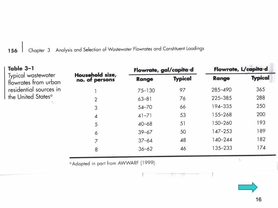
Domestic Wastewater Sources and Flow rates:

• Residential Areas : Table 3-1

• Commercial Districts: Generally expressed in gal/acre.d

(m3/ha.d) range form 800 – 1500 gal/acre.d (Table 3-2)

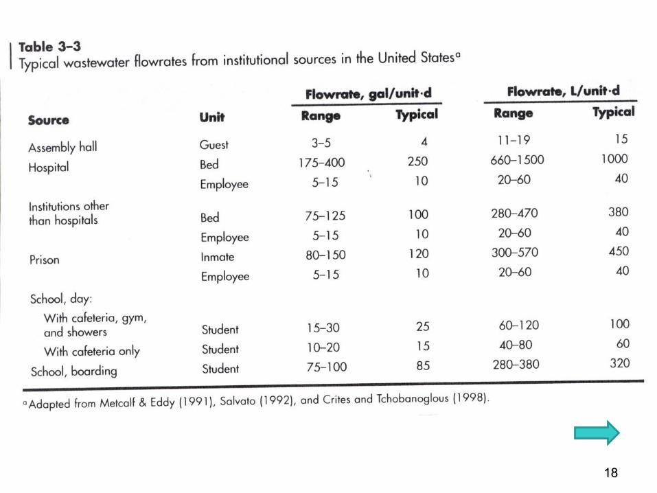
• Institutional facilities Table 3-3

• Recreational (highly seasonal) facilities Table 3-4

Industrial Wastewater Sources and Flow rates:

Range:

• 1000 –1500 gal/acre.d light industrial development

• 1500–3000 gal/acre.d medium industrial development

• 85-95% of water use industries without internal water reuse

• For large industries separate estimates must be made.

5

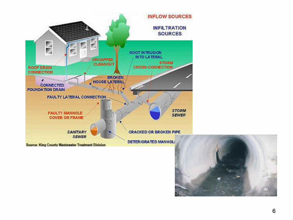
Wastewater sources and flow rates

Infiltration/Inflow (I/I)

• Infiltration defective pipes ----etc.

• Steady inflow from cellar and foundation drains, etc.

• Direct inflow from direct storm water runoff connections to

sanitary sewer possible source are roof leaders, yard drains,

manhole covers.

• Total inflow direct + upstream flow (overflows/pumping

stations bypasses)

• Delayed inflow storm water that requires several days to

drain through manholes, etc…..

Infiltration flowrate:

• The amount of water that can enter a sewer from groundwater

(or infiltration) ranges from 100 - 10,000 gal/d. in-mi .

• Or 20 – 3000 gal/acre.d. (Example 3-2)

6

7

Statistical Analysis of flowrates, constituent concentrations, and mass loadings

Statistical analysis involves the determination of statistical

parameters used to quantify a series of measurements.

Important in developing wastewater management systems

Common statistical parameters:

• In normal distribution, data is described using: mean, median,

mode, standard deviation, and coefficient of variation. Table 3-10

• In skewed distribution, data is described using log of

the value of the normal distribution (geometric). Table 3-10

Graphical analysis of data:

• Used to determine the nature of distribution: plotting

data on both arithmetic and log-probability papers.

Examples 3-4 and 3-5

9

Analysis of flowrate data

Because the hydraulic design of both collection and treatment facilities is

affected by variation in wastewater flowrates, it is important that the

flowrate characteristics be carefully analyzed.

Definition of terms: (Table 3-11)

Variations in wastewater flowrates.

• Short term variations: (Figure 3-4).

• Seasonal variations.

• Industrial variations.

Wastewater flowrate factors:

• Maximum flows are determined by peaking factor (PF).

•

flowrate term-long average

daily)hourly, (e.g., flowrate peakPF

10

Analysis of constituent mass loading

• BOD and TSS mass loadings can vary up to two or

three times the average conditions.

• Design of wastewater treatment processes should

consider peak conditions.

Quantities of waste discharged: (Table 3-12)

• Typical BOD5 (not including kitchen waste) is .18

Ib/cap.d.

• Example:

Given: a town of 125,000 population. Estimate the BOD5 loading of

the raw wastewater

BOD5 = .18 x 125,000 cap= 22,500 lb/day

cap.d

Ib

11

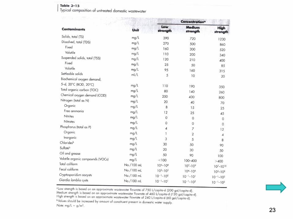
Analysis of constituent mass loading

Composition of Wastewater in Collection Systems.

• T3-15, p. 186. The values are based on 120 ,which is the

suggested EPA flow.

• Example: The average flow is 120 and the average BOD5 is

190 mg/l. What is the BOD5 loading in

• = Conc. (mg/l) x 8.34 x Q(MGD)

• = 190 x 8.34 x 120 x

• = .19 which aggress with value stated in T3-12, p.182.

cap.d

gal

cap.d

Ib

cap.d

gal

cap.d

Ib

mg/l

Ib/MG

cap.d

Ib

L

mg

mg/l

Ib/MG

cap.d

gal

gal10

MG6

cap.d

Ib

12

Analysis of constituent mass loading

Short term variation in constituent values.

• Figure 3-6: Typical hourly variations in flow and strength of

wastewater.

Variations in industrial wastewater.

• Composition is highly variable depending on industry type.

• Concentrations (BOD, TSS) vary significantly throughout the day.

• Pre-treatment may be required before discharge to municipal

sewer.

13

Design flowrates and mass loadings

Average daily flow

• It is the average flow occurring over a 24-hour period under dry

weather conditions.

• used in evaluating plant capacity, estimating pumping and

chemical cost, sludge production, organic loading rates

Maximum daily flow

• It is the maximum flow on a typical dry weather diurnal flow curve.

• used for the design of facilities involving retention time, such as:

– Equalization basins and Chlorine Contact Tanks

Minimum daily flow

• It is the minimum flow on a typical dry weather diurnal flow curve.

• used in sizing of conduits for minimum deposition

14

Design flowrates and mass loadings

Peak hourly flow

• The peak hourly flow occurs during or after precipitation and

includes a substantial amount of I/I.

• used for the design of

– Collection and interceptor sewers

– Pumping stations

– Flow meters, grit chambers, conduits, channels in plant

• Peak Flowrate Factors may be projected using Figure 3-13,

p.202.

Minimum hourly flow

• It is the lowest flow on a typical dry weather diurnal flow curve.

• used in sizing wastewater flowmeters, wastewater pumping

15

Design flowrates and mass loadings

Mass loading:

• Table 3-20

• Important in the design of treatment facilities such as:

– Sizing aeration tanks.

– Biosolids processing facilities (Biosolids produced are directly related to BOD mass loading)

– Oxygen requirements are affected by mass loading

16

17

18

19

20

21

22

23

24

25

Origin of waste

Biochemical oxygen

demand

“BOD” (kg/ton

product)

Total Suspended

solids

“TSS” (kg/ton

product)

Domestic sewage 0.025

(kg/day/person)

0.022

(kg/day/person)

Dairy industry 5.3 2.2 Yeast industry 125 18.7 Starch & glucose industry 13.4 9.7 Fruits & vegetable canning

industry 12.5 4.3

Textile industry 30 - 314 55 - 196 Pulp & paper industry 4 - 130 11.5 - 26 Beverage industry 2.5 - 220 1.3 - 257

* Rapid assessment for

industrial pollution

Tannery industry

48 - 86 85 - 155

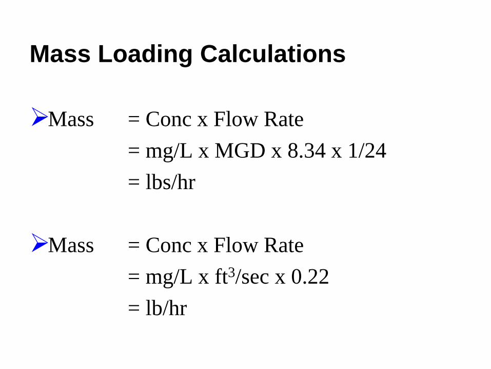
Mass Loading Calculations

Mass = Conc x Flow Rate

= mg/L x MGD x 8.34 x 1/24

= lbs/hr

Mass = Conc x Flow Rate

= mg/L x ft3/sec x 0.22

= lb/hr

Mass Balance Calculations

Fundamental Law: Massin = Massout

Massin = Q1 x Conc1 + Q2 x Conc2 (knowns)

Massout = QT x ConcT

(unit constants cancel out)

QT = Q1 + Q2

ConcT = unknown

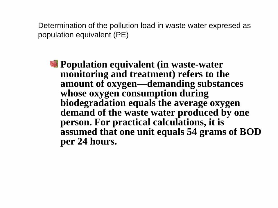
Determination of the pollution load in waste water expresed as

population equivalent (PE)

Population equivalent (in waste-water monitoring and treatment) refers to the amount of oxygen—demanding substances whose oxygen consumption during biodegradation equals the average oxygen demand of the waste water produced by one person. For practical calculations, it is assumed that one unit equals 54 grams of BOD per 24 hours.

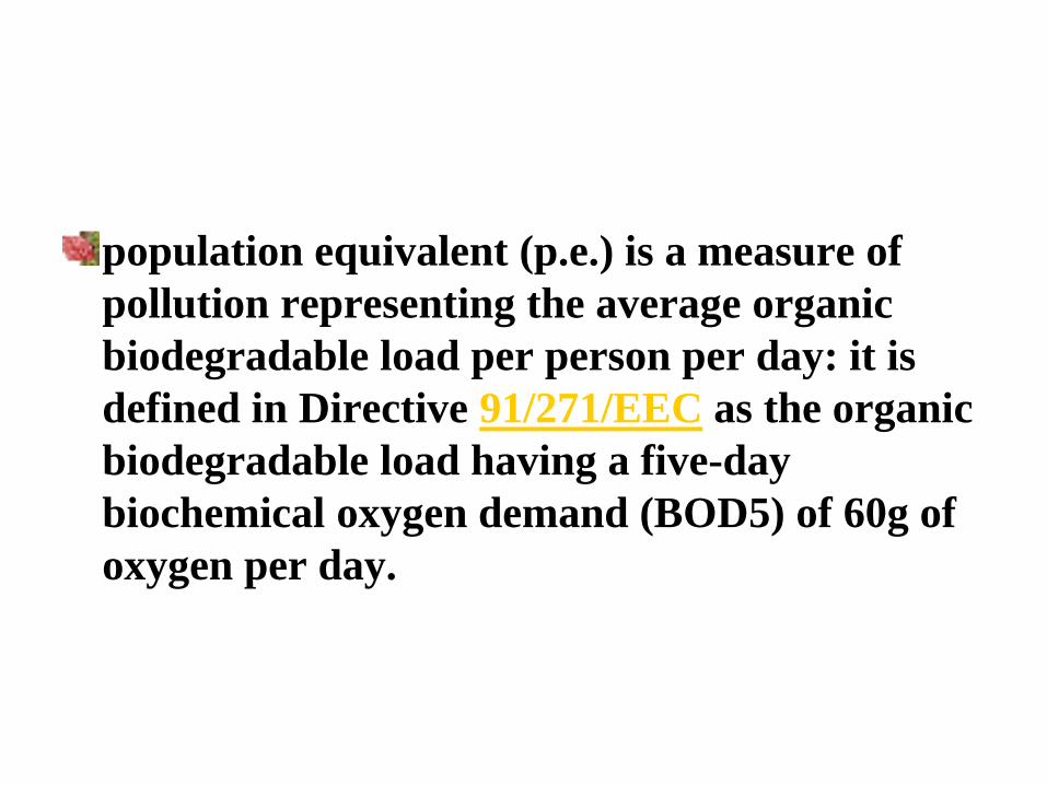
population equivalent (p.e.) is a measure of

pollution representing the average organic

biodegradable load per person per day: it is

defined in Directive 91/271/EEC as the organic

biodegradable load having a five-day

biochemical oxygen demand (BOD5) of 60g of

oxygen per day.

Determination of the pollution load in waste

water expresed as population equivalent (PE)

Site works – 48 h:

Meauserment of flow every 15 minutes

Sampling every 15 minutes to prepare 2 h composite samples

Meauserment of temperature every 2 h

Population Equivalents

1. Wastewater discharge: 100 -120 gpcd

- 70 gpcd domestic

- 10 gpcd industrial/commercial

- 20 to 40 gpcd infiltration

2. Suspended Solids and BOD

SS = 0.2 lb pcd (without kitchen grinder)

SS = 0.22 lb pcd (with kitchen grinder)

BOD = 0.17 lb BOD pcd

BOD = 0.26 lb BOD pcd (with kitchen grinder)

Population Equivalents cont.

For 100 gpcd and consider for one person:

BOD0.17 lb

100 gal

1

8.34 lb

106

galmg

L

BOD 204mg

L

SS0.2 lb

100 gal

1

8.34 lb

106

galmg

L

SS 240

mg

L

Population Equivalents cont.

Used to

• Establish population equivalency of an industrial waste.

• Establish charge for treating industrial waste based on BOD or SS rather than flow.

Find the BOD and flow equivalent for an industrial waste

with the following characteristics:

Q 0.1MGDMGDMGD BOD 450mg

L

Flow:0.1MGD

100 gal

person day

1000peoplepeoplepeople

BOD: 0.1MGD 450 mg

L

8.34 lb

MGDmg

L

0.17 lb BOD

person day

2208peoplepeoplepeople

BOD equivalent is 2.2 times greater than flow equivalent.

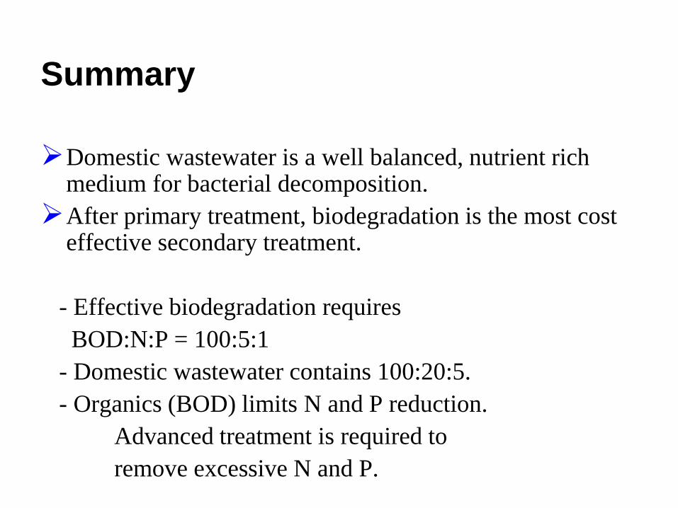
Summary

Domestic wastewater is a well balanced, nutrient rich medium for bacterial decomposition.

After primary treatment, biodegradation is the most cost effective secondary treatment.

- Effective biodegradation requires

BOD:N:P = 100:5:1

- Domestic wastewater contains 100:20:5.

- Organics (BOD) limits N and P reduction.

Advanced treatment is required to

remove excessive N and P.