Embed Size (px)
Citation preview
1
MEE09:53
__________________________________________________________
Analysis and simulation of channel equalization in TDD-CDMA
Muhammad Adnan Khan
840226-6871 [email protected]
&
Naseer-Ud-Din Shinwari 820301-8117
This thesis is presented as part of Degree of Master of Science in Electrical Engineering
Blekinge Institute of Technology August 2009
__________________________________________________________ Blekinge Institute of Technology School of Engineering Department of Applied Signal Processing Supervisor: Dr. Jörgen Nordberg Examiner: Dr. Jörgen Nordberg

2
3
Abstract
The field of telecommunications has made tremendous progress of the past decade, especially in
the area of wireless communications. The world becoming a global village due the advancement
in the field of wireless communications, the requirement for standardization and uniformity
becomes an essential issue. CDMA is the efficient technology that has emerged in the last decade
and has revolutionized the pre-existing mobile communication concepts. CDMA is a spread
spectrum-based technique for multiplexing, that provides and alternative to TDMA for Second
Generation cellular networks.
In FDD-CDMA the uplink and downlink transmissions use two separate frequency bands for
duplex transmission. It would be correct to call TDD-CDMA as one of the flavors of CDMA
technology and has taken the concept to a whole new level of performance, simplicity and cost
effectiveness. In TDD-CDMA, the uplink and downlink transmissions use the same frequency
band for duplex transmission by using synchronized time intervals. The TDD-CDMA
(TD_CDMA) is very similar to FDD CDMA on all of its higher-level functionality. The major
differences are in the physical layer, where TDD-CDMA combines TDMA and CDMA elements
while FDD-CDMA combine FDMA and CDMA elements.
This Research will focus on different features of TDD-CDMA and implementing channel
equalization in Matlab.
Channel equalization: In channel Equalization we implement the channel estimation algorithm
to equalize the channel and reduce the BER in the received signal. The Channel equalization is
carried out at the receiver.

4

5
Acknowledgment
All the praises to our Al-Mighty ALLAH who blesses us and gives us the power of knowledge
that we successfully finished our thesis.
First and most importantly we would like to thanks our supervisor Dr. Jorgen Nordberg for his
support, guidance and interest in our work efforts during the development of this thesis. Then we
would like to say special thanks to our program Manager Mr. Mikeal Asman, professor Claes
jogreus and student coordinator Miss Lena Magnusson for their unlimited cooperation and help.
We would like to thanks our friends for their moral support during this thesis work
We dedicated this thesis to our parents for their endless support and unlimited prayers for our
success.
6
Table of contents
Abstract………………………………………………………………………………………………………………. 3
Acknowledgement…………………………………………………………………………………………………….5
Table of contents……………………………………………………………………………….. ……………………6
List of Figures………………………………………………………………………………………………………..10
List of Tables………………………………………………………………………………………………………...12
Chapter -1 Introduction
1.1. Thesis Objective………………………………………………………………………………………………….13
1.2. Generations of Cellular Systems…………………………………………………………………………………13
1.2.1. First Generation Cellular Systems............................................................................................................13
1.2.2. Second Generation Cellular Systems........................................................................................................14
1.2.3. Third Generation Cellular Systems.............................................................................................................14
1.3. Multiple Access Techniques…………………………………………………………………………………….16
1.3.1. Frequency Division Multiple Access (FDMA)............................................................................................16
1.3.2. Time Division Multiple Access (TDMA)...................................................................................................16 1.3.3. Code Division Multiple Access (CDMA)………………………………………………………………...17
1.4. Spread Spectrum Multiple Access …………………………………………………………………………….18
1.4.1 Direct Sequence Spread Spectrum (DSSS)……………………………………………………………..18
1.5. Thesis outlines…………………………………………………………………………………………………19
Chapter -2 TDD-CDMA
2.1. Basic TDD Principles…………………………………………………………………………………………….20
2.2. TDD-CDMA commercial standards……………………………………………………………………………..23
2.2.1. TD-CDMA...............................................................................................................................................24
2.2.2. TD-SCDMA.............................................................................................................................................24
2.3. TD-SCDMA Frame Hierarchy …………………………………………………………………………………..25
2.3.1. TD-SCDMA Frame Structure…………………………………………………………………………25
2.4. TD-SCDMA Slot Structure………………………………………………………………………………………26
7
2.5. TD-SCDMA Synchronization Slots.......................................................................................................................27
2.5.1. Downlink Pilot Time Slot (DwPTS)…………………………………………………………………..27
2.5.2. Uplink Pilot Time Slot (UpPTS)………………………………………………………………………27
2.5.3. Guard Period (G)………………………………………………………………………………………28
2.6. TD-SCDMA Channels…………………………………………………………………………………………...28
2.6.1. Transport channels………………………………………………………………………………………..28
2.6.2. Physical channels…………………………………………………………………………………………28
2.7. Spreading and Scrambling……………………………………………………………………………………..29
2.7.1. Walsh Codes……………………………………………………………………………………………29
2.7.2. Scrambling Codes………………………………………………………………………………………31
2.8. TDD-CDMA Receiver structure………………………………………………………………………...…….33
Chapter-3 System Model
3.1. Simulation Model……………………………………………………………………………………………...35
3.2. Transmitter Module……………………………………………………………………………………………37
3.2.1. Random data generator………………………………………………………………………………….37
3.2.2. Walsh Code Spreading………………………………………………………………………………….37
3.2.3. PN Code Scrambling……………………………………………………………………………………38
3.2.4. Digital Modulation……………………………………………………………………………………...38
3.2.4.1. Amplitude-Shift Keying (ASK)…………………………………………………………..38
3.2.4.2. Frequency-Shift Keying (FSK)…………………………………………………………..39
3.2.4.3. Phase-Shift Keying (PSK)…………………………………………………………….....39
3.3. Binary Phase Shift Keying (BPSK)……………………………………………………………………............39
3.4. Quadrature Phase Shift Keying (QPSK)……………………………………………………………….……...40
3.5. Quadrature Amplitude Modulation……………………………………………………………………………40
3.6. Channel Module……………………………………………………………………………………………….41
8
3.6.1. Multipath delay spread…………………………………………………………………………….42
3.6.2. Fading characteristics……………………………………………………………………...……….42
3.6.3. Path loss……………………………………………………………………………………….…...42
3.6.4. Doppler spread……………………………………………………………………………………..42
3.6.5. Co-channel interference……………………………………………………………………………43
3.7. Additive White Gaussian Noise (AWGN) Channel…………………………………………………………..43
3.8. Stanford University Interim (SUI) Channel Model…………………………………………………………...44
3.8.1. Input Mixing Matrix…………………………………………………………………………44
3.8.2. Tapped Delay Line (TDL) Matrix…………………………………………………………...45
3.8.3. Output Mixing Matrix………………………………………………………………………..45
3.9. Receiver Module………………………………………………………………………………………………46
3.9.1. BPSK Demodulation………………………………………………………………………………...47
3.9.2. PN Code Descrambling………………………………………………………………………………47
3.9.3. Walsh Decoding……………………………………………………………………………………...47
3.9.4. Adaptive Channel equalization……………………………………………………………………….47
3.9.5. Diversity Combiner…………………………………………………………………………………..47
3.9.6. Integrated Circuit and Decision Threshold…………………………………………………………...48
Chapter-4 Channel Estimation Algorithms
4.1. Channel estimation…………………………………………………………………………………………….49
4.2. Optimal Adaptive Maximum Likelihood Sequence Estimation (MLSE) Algorithm........................................50
4.3. Adaptive Minimum Mean Square Error (MMSE) Algorithm ……………………….………..........................50
4.3.1. Optimal MMSE Receiver………………………………………………………………...50
4.3.2. Sub optimal MMSE Receiver…………………………………………………………………………50
4.3.2.1. The Least Mean Squares (LMS) Algorithm……………………………………………….50
9
4.3.2.2. The Recursive Least squares (RLS) Algorithm……………………………………………52
4.4. Choice of Algorithm…………………………………………………………………………………………...52
Chapter -5 Simulation Results
5.1. Simulation Environment………………………………………………………………………………………..53 5.2. SISO (Single Input Single Output)…………………………………………………………………………….55
5.2.1 AWGN Channel Performance…………………………………………………………………………55
5.2.2 SUI-3 Channel Performance…………………………………………………………………………..57
5.3. SIMO (Single Input Multiple Output)…………………………………………………………………………59
5.3.1. Performance of Optimal and Sub Optimal Receiver………………………………………………...59
Chapter-6 Conclusion and Future Work
5.1. Conclusion………………………………………..……………………………………………………………63
5.2. Future work……………………………………………………………………………………………………64
References………………………………………………………………………………………………………....65
10
List of Figures
Figure1.1 FDMA bandwidth spectrum
Figure.1.2 TDMA frames structure.
Figure.1.3 Multiple Acces Techniques.
Figure .1.4 Principles of DS-SS.
Figure 2.1 TDD and FDD duplexing mode.
Figure 2.2 Uplink and downlink time slots.
Figure 2.3 Unequal slot lengths.
Figure 2.4 Number of Uplink and downlink time slots per frame
Figure 2.5 Frequency Plan.
Figure 2.6 The TD-SCDMA time frame hierarchy.
Figure 2.7 Symmetric DL/UL Allocation.
Figure 2.8 Asymmetric DL/UL Allocation.
Figure 2.9 the TD-SCDMA Slot Structure.
Figure 2.10 Burst structure of DwPTS.
Figure 2.11 Burst structure of UpPTS.
Figure 2.12 Hadamard matrix of 2x2 order
Figure 2.13 Code-Tree for Generation of OVSF.
Figure 2.14 Generation of OVSF matrix equation.
Figure 2.15 Multistage shift register to generate a PN code.
Figure 2.16 Rake receiver supported by TDD-CDMA
Figure 3.1.Complete Simulation Model
11
Figure 3.2 Transmitter Module
Figure 3.3 BPSK constellations
Figure 3.4 QPSK constellations
Figure 3.5 8-QAM constellations
Figure 3.6 16-QAM constellations
Figure 3.7 Co-channel Interference Scenario
Figure 3.8 AWGN Channel
Figure 3.9 Structure of SUI-3 channel model
Figure 3.10 Receiver Module
Figure 4.1 General Adaptive channel estimation
Figure 5.1 BPSK in AWGN
Figure 5.2 QPSK in AWGN
Figure 5.3 8-QAM in AWGN
Figure 5.4 BPSK in SUI-3
Figure 5.5 QPSK in SUI-3
Figure 5.6 8-QAM in SUI-3 Figure 5.7 Optimal and Sub Optimal Receiver in BPSK Figure 5.8 Optimal and Sub Optimal Receiver in QPSK Figure 5.9 Optimal and Sub Optimal Receiver in 8-QAM
12
List of Tables
Table 1.1 Comparison of various cellular standards.
Table 2.1 Transport and Physical channel mapping.
Table 3.1 SUI-3 channel model definition
Table 4.1 SNR required to get BER level at 10 -0.44
Table 4.2 BER level at SNR=10 for Optimal and Sub Optimal Receiver
Table 4.3: BER at SNR=10 dB
Table 4.4 SNR loss in dB at BER level 0.01
13
Chapter 1- Introduction
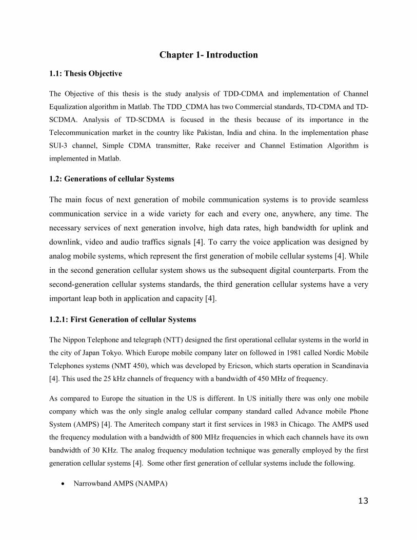
1.1: Thesis Objective
The Objective of this thesis is the study analysis of TDD-CDMA and implementation of Channel
Equalization algorithm in Matlab. The TDD_CDMA has two Commercial standards, TD-CDMA and TD-
SCDMA. Analysis of TD-SCDMA is focused in the thesis because of its importance in the
Telecommunication market in the country like Pakistan, India and china. In the implementation phase
SUI-3 channel, Simple CDMA transmitter, Rake receiver and Channel Estimation Algorithm is
implemented in Matlab.
1.2: Generations of cellular Systems
The main focus of next generation of mobile communication systems is to provide seamless
communication service in a wide variety for each and every one, anywhere, any time. The
necessary services of next generation involve, high data rates, high bandwidth for uplink and
downlink, video and audio traffics signals [4]. To carry the voice application was designed by
analog mobile systems, which represent the first generation of mobile cellular systems [4]. While
in the second generation cellular system shows us the subsequent digital counterparts. From the
second-generation cellular systems standards, the third generation cellular systems have a very
important leap both in application and capacity [4].
1.2.1: First Generation of cellular Systems
The Nippon Telephone and telegraph (NTT) designed the first operational cellular systems in the world in
the city of Japan Tokyo. Which Europe mobile company later on followed in 1981 called Nordic Mobile
Telephones systems (NMT 450), which was developed by Ericson, which starts operation in Scandinavia
[4]. This used the 25 kHz channels of frequency with a bandwidth of 450 MHz of frequency.
As compared to Europe the situation in the US is different. In US initially there was only one mobile
company which was the only single analog cellular company standard called Advance mobile Phone
System (AMPS) [4]. The Ameritech company start it first services in 1983 in Chicago. The AMPS used
the frequency modulation with a bandwidth of 800 MHz frequencies in which each channels have its own
bandwidth of 30 KHz. The analog frequency modulation technique was generally employed by the first
generation cellular systems [4]. Some other first generation of cellular systems include the following.
• Narrowband AMPS (NAMPA)
14
• Total Access Cellular Systems (TACS)
• Nordic mobile Telephone Systems (NMT)
1.2.2: Second Generation Cellular Systems
Due to the fast growing numbers of subscriber and the reproductions of lots of not compatibility to first
generation cellular systems was the important reason to move towards the next or second-generation
cellular systems [4]. Due to the good coding technique associated with digital technology the second
generation cellular systems has many advantages over the first generation cellular systems [4]. The main
difference between the first and second generation is that all the second-generation cellular systems has
employ the digital modulation schemes. Code Division Multiples Access (CDMA) and Time Division
Multiple Access (TDMA) used in second generation cellular systems along with FDMA [4]. The Second
generation consists on the following cellular techniques, which are following:
• United States Digital Cellular (USDC) Standards IS–54 and S-136
• Global System for Mobile Communication (GSM)
• Pacific Digital Cellular (PDC)
• Cdma-One
1.2.3: Third Generation cellular Systems
In 1999 the mobile communication describes the characteristic by a diverse set of application using
different standards of not compatible around the whole world [4]. Now a day the mobile communication
is truly use a personal communication, to make the standard and application more strong and secure. The
ultimate goal of all this purpose is to define a new generation known as third generation mobile radio
standard [4]. Initially which was knows as Future Public Land Mobile Telecommunications Systems
(FPLMTS). This was renamed recently with IMT – 2000 for international Mobile Telecommunications.
Third generation cellular system is more suitable for multimedia application such as high speed Internet,
video calling and video conferencing. To keep this target in mind International Telecommunication Union
(ITU) the standard committees in Europe, Japan, United States, South Korea and China, submitted
different evaluation proposals. The Wideband CDMA (WCDMA) was developed on a standard based
common technology by different countries.
15
Table 1.1 shows the Comparison of various cellular standards [4].
NAME AMPS GSM/DCS –1900 IS – 136 USDC IS-95 CDMA2000 WCDMA/UTRA
Generation 1 2 2 2 3 3
Year introduced & origin
1983
US
1992/1994
Germany
1996
US
1993
US
2002
US
2002
Europe
Frequency Band
Uplink (MHz)
Downlink (MHz)
824-849
869-894
Cellular /PCS
890-915/
1850-1910
935-960/
1930-1990
Cellular/PCS
824-849/
1850-1910
869-894/
1930-1990
Cellular/PCS
824-849/
1850-1910
869-894/
1930-1990
PCS
1850- 1910
1930- 1990
1920 – 1980
2110 - 2170
Multiple Access Scheme
FDMA TDMA TDMA CDMA CDMA CDMA
Bandwidth per Channel
30 kHz 200 kHz 30 kHz 1.25 MHz 1.25,3.75, 7.5,
11.25, 15 MHz
5, 10, 20 MHz
Modulation type FM GMSK π/4 - DPSK QPSK and OQPSK
QPSK and BPSK
QPSK and BPSK
Max. output power
Base:
Mobile:
20W
4W
320 W
8 W
20W
4 W
64 kW**
6.3 W
1.64 kW**
2 W
Unspecified
1 W
Users/Channel 3 8 3 Up to 63 Up to 253 Up to 250
Data Rate 19.2 kbps*
22.8 kbps 13 kbps 19.2 kbps 1.5 kbps to
2.0736 Mbps
100 bps to
2.048 Mbps
Region of Coverage US Europe, India,
US (PCS)
US US, Hong Kong,
Middle-East, Korea
US Europe
TABLE 1.1 Comparison of various cellular standards [4].
16
1.3: Multiple Access Techniques
In Multiple Access technique more than one user at the same time uses the available bandwidth [1]. It is
always seems that the bandwidth allocation is very limited in a radio systems. In order to increase the
capacity of user of any wireless network multiple access techniques is used. FDMA, TDMA and CDMA
are used to share the available bandwidth among the multiple users in a wireless networks [1].
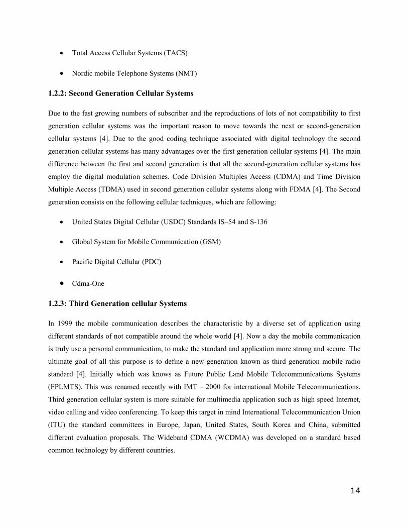
1.3.1: Frequency Division Multiple Access (FDMA)
In Frequency Division Multiple Access (FDMA), the available spectrum is divided into a number of
small and equal size bandwidth slots, which was assigned for user at different time when they need to call
[1]. Now that user can only use this frequency only at that time and no other can use this frequency nor
can it be allocate to any other user [1]. Each user is allocated two frequencies band called uplink channel
and downlink channel. Forward channel is used for transmission from base station to mobile phone while
downlink channel is used for transmission from mobile phone to base station. Generally the bandwidth in
FDMA system is low because only one user will used it at the same time. There is a space between two
adjacent frequencies, which is called guard band. Guard band is used to remove interference between
adjacent frequencies [1]. Figure 1.1 shows the FDMA bandwidth spectrum [1]
Guard band
Individual
Channel
Figure 1.1 FDMA bandwidth spectrum [1].
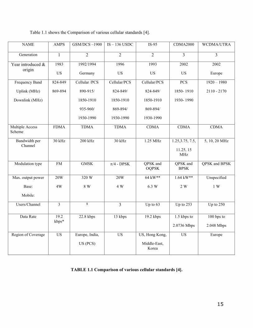
1.3.2: Time Division Multiple Access (TDMA)
Using TDMA the available bandwidth is divided in two a number of equal time slots and available for the
users when they needed [1]. User can send and receive data using these time slots. Any user can be assign
one or more time slots depend on the need of the user and user is only allowed to use its allocated slots in
the channels of different slots [1]. Like FDMA there is also a guard period. Guard period is used to
overcome the inter symbol interference between different signals. Figure 1.2 shows the Frame structure of
TDMA [1]
17
Guard Period
Slot 1 Slot 2 0 0 0 Slot N
time
Frame
Figure 1.2 TDMA frames Structure [1].
In TDMA a buffer techniques is used. The transmission is not continuous in TDMA it is buffered before
to send that’s why a buffer and burst techniques are used [1] [2]. In TDMA system the input data is first
buffered and then send to the destination end. Due to buffering this technique cannot be used in analog
data transmission, it is more suitable for digital transmission.
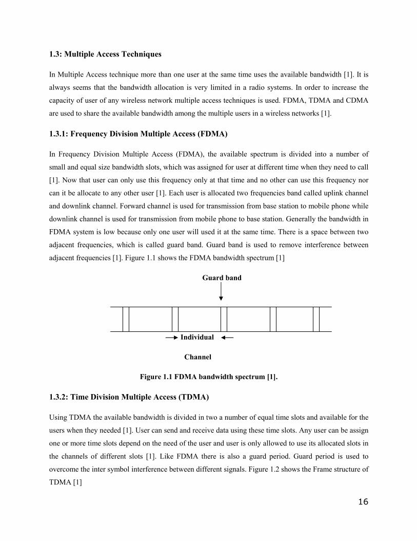
1.3.3: Code Division Multiple Access:
Code Division Multiple Access (CDMA) is different technique from both TDMA and FDMA. Because in
this technique there is no allocation of any frequency band or time slots. CDMA is a spread spectrum
technique used for multiplexing [2]. This technique is used as an alternative for TDMA in second-
generation cellular system. In CDMA a random generated code called pseudo random noise code (PN
code), which generates PN code for each and every user in the same channel, and at the receiver end each
user can be select on the basis of that PN code [2]. CDMA technology was solely used for military
applications for so many years. Figure 1.3 shows the Multiple Access Techniques i.e. FDMA, TDMA and
CDMA [2].
Figure 1.3 Multiple Access Techniques [2].
18
1.4: Spread spectrum multiple access
In spread spectrum multiple access technique all the users have the access to use and transmit their data
simultaneously on the whole available bandwidth using a special code called pseudorandom code [3].
Each user has unique PN code. PN code is generated randomly with help of multistage shift registers.
These code sequences repeat itself after some specific number of times. On the destination end the
receiver can separate these codes by correlating the received single with help of this combination of codes
[3].
There are different kinds of spread spectrum techniques available, direct sequence spread spectrum
(DSSS), frequency hopping spread spectrum (FHSS), and Time hopping spread spectrum (THSS) [3]. We
will only discus the spread spectrum techniques because this technique is used in CDMA2000, UMTS
and W-CDMA.
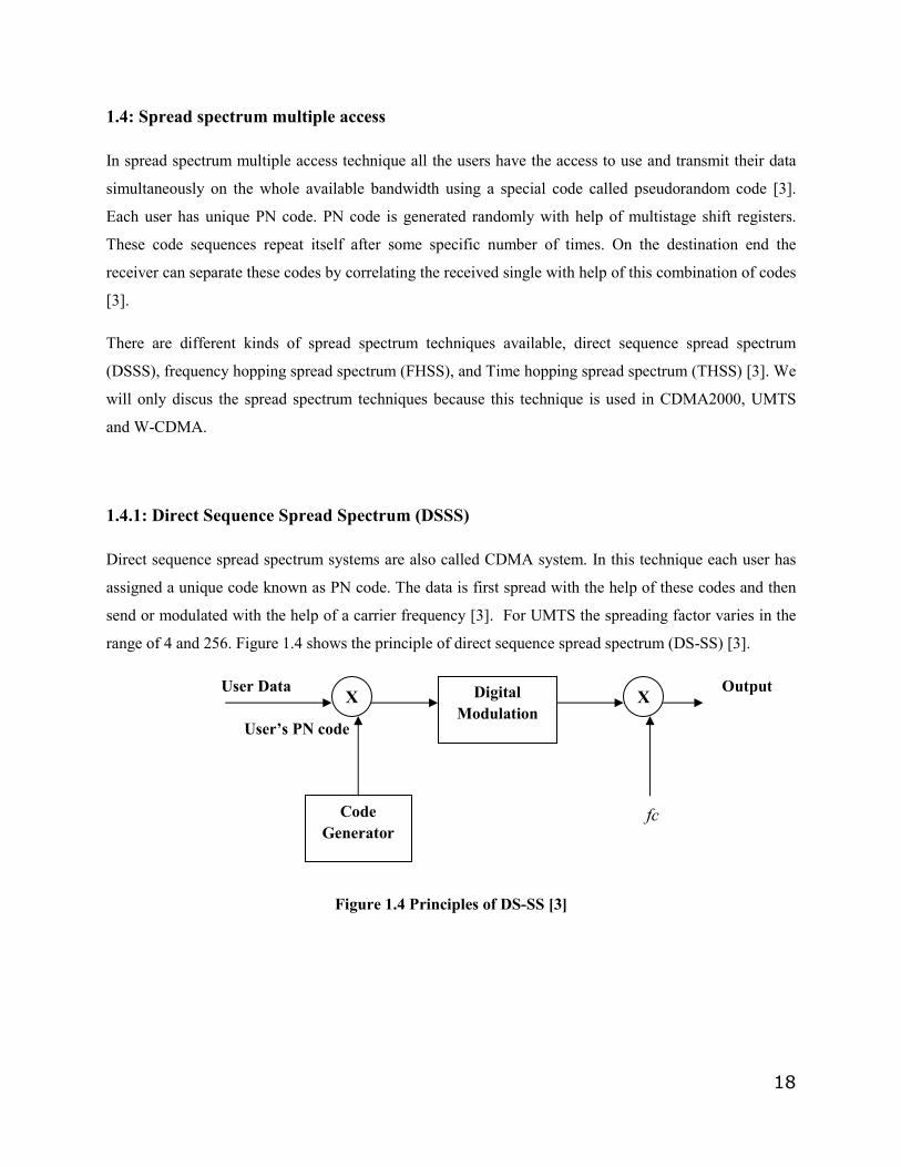
1.4.1: Direct Sequence Spread Spectrum (DSSS)
Direct sequence spread spectrum systems are also called CDMA system. In this technique each user has
assigned a unique code known as PN code. The data is first spread with the help of these codes and then
send or modulated with the help of a carrier frequency [3]. For UMTS the spreading factor varies in the
range of 4 and 256. Figure 1.4 shows the principle of direct sequence spread spectrum (DS-SS) [3].
User Data Output
User’s PN code
fc
Figure 1.4 Principles of DS-SS [3]
X Digital Modulation
X
Code Generator
19
1.5: Thesis Outlines
Chapter 2 provides the theoretical back ground about TDD Duplexing scheme, TDD-CDMA Commercial
standards like TD-CDMA and TD-SDMA and the features offered by TD_SCDMA like TD-SCDMA
Frame Hierarchy, Slot Structure, Synchronization Slots, Transport and physical channels, Walsh Codes
and scrambling codes.
Chapter 3 focuses on System model. In the simulation model we describe how our system works by a
flow chart.
Chapter 4 focuses on channel estimation algorithms.
Chapter 5 is all about the Simulation results. Comparison of the Theoretical BER of the system verses
simulated BER of the system (BPSK, QPSK and 8-QAM) using AWGN channel is shown by the graphs.
Comparison of the Theoretical BER of the system verses simulated BER of the system (BPSK, QPSK and
8-QAM) using SUI-3 channel is shown by the graphs. Comparison of Optimal and Sub Optimal receiver
is also shown by the graphs
Chapter 6 is all about the conclusion of the thesis work followed by future work.
20
Chapter 2: TDD CDMA
2.1: Basic TDD Principle
Transmission between two users is called communication and this communication is either simplex or
duplex. Simplex is a one-way communication while duplex is a two-way communication. Two-way
transmissions between two users can be achieved in different ways. The most common method used is
frequency division duplex (FDD) transmission. In FDD communication two different frequencies are
using for duplex transmission. While this two-way communication has been accomplished in TDD by
different time slot but the frequency will remain the same. In this chapter we will discuss the TDD
operation in CDMA and how can we differentiate TDD and FDD operations modes from each other.
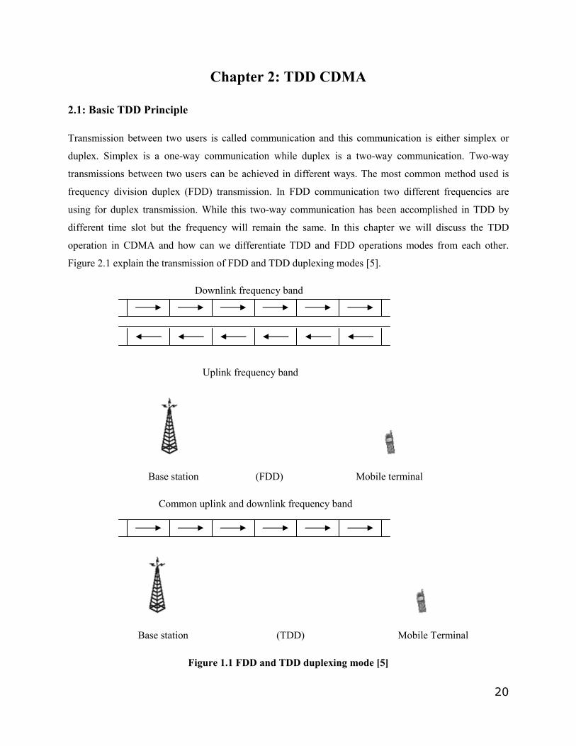
Figure 2.1 explain the transmission of FDD and TDD duplexing modes [5].
Downlink frequency band
Uplink frequency band
Base station (FDD) Mobile terminal
Common uplink and downlink frequency band
Base station (TDD) Mobile Terminal
Figure 1.1 FDD and TDD duplexing mode [5]
21
In the above figure two modes FDD and TDD differ from each other in the data transmission over mobile
communication systems [5]. In FDD mode a separate frequencies bands is used for uplink and downlink
transmission [5]. A guard frequency is used to prevent inter symbol interference between two signals.
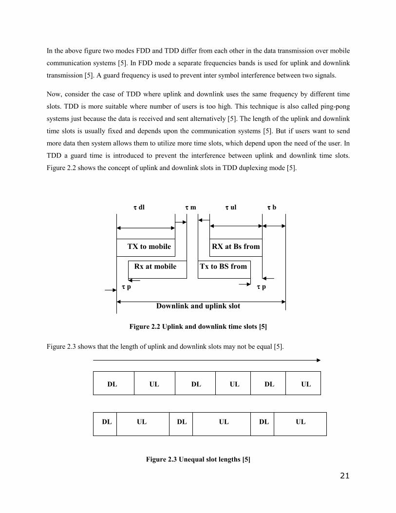
Now, consider the case of TDD where uplink and downlink uses the same frequency by different time
slots. TDD is more suitable where number of users is too high. This technique is also called ping-pong
systems just because the data is received and sent alternatively [5]. The length of the uplink and downlink
time slots is usually fixed and depends upon the communication systems [5]. But if users want to send
more data then system allows them to utilize more time slots, which depend upon the need of the user. In
TDD a guard time is introduced to prevent the interference between uplink and downlink time slots.
Figure 2.2 shows the concept of uplink and downlink slots in TDD duplexing mode [5].
τ τ τ τ dl τ τ τ τ m τ τ τ τ ul τ τ τ τ b
TX to mobile RX at Bs from
Rx at mobile Tx to BS from
τ τ τ τ p τ τ τ τ p
Downlink and uplink slot
Figure 2.2 Uplink and downlink time slots [5]
Figure 2.3 shows that the length of uplink and downlink slots may not be equal [5].
DL UL DL UL DL UL
DL UL DL UL DL UL
Figure 2.3 Unequal slot lengths [5]
22
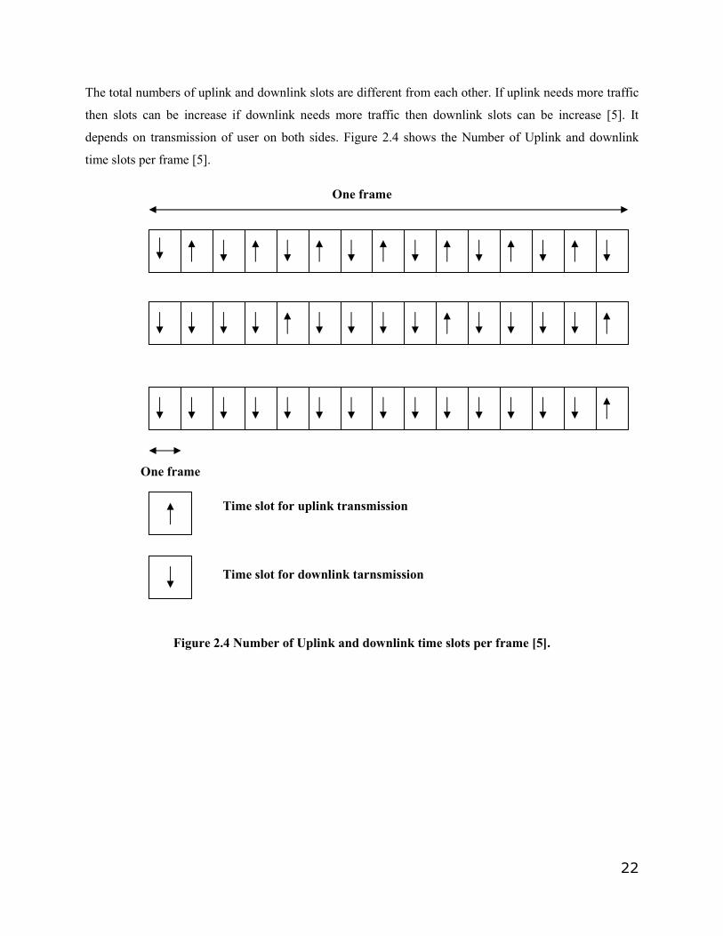
The total numbers of uplink and downlink slots are different from each other. If uplink needs more traffic
then slots can be increase if downlink needs more traffic then downlink slots can be increase [5]. It
depends on transmission of user on both sides. Figure 2.4 shows the Number of Uplink and downlink
time slots per frame [5].
One frame
One frame
Time slot for uplink transmission
Time slot for downlink tarnsmission
Figure 2.4 Number of Uplink and downlink time slots per frame [5].
23
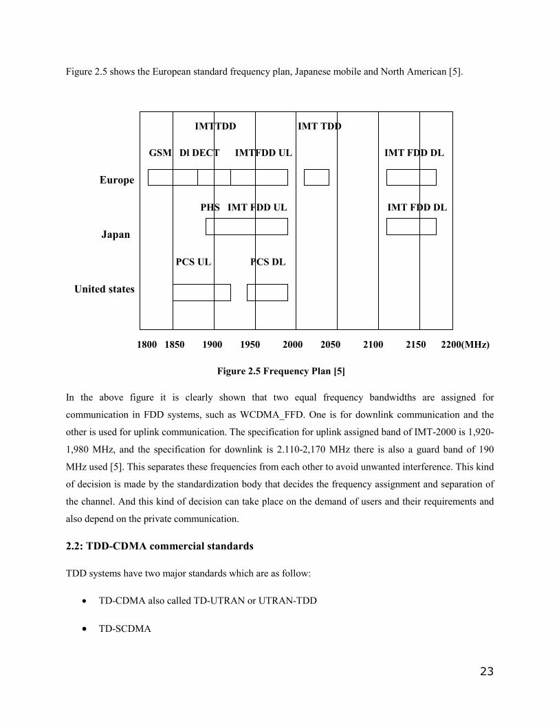
Figure 2.5 shows the European standard frequency plan, Japanese mobile and North American [5].
IMTTDD IMT TDD
GSM Dl DECT IMTFDD UL IMT FDD DL
Europe
PHS IMT FDD UL IMT FDD DL
Japan
PCS UL PCS DL
United states
1800 1850 1900 1950 2000 2050 2100 2150 2200(MHz)
Figure 2.5 Frequency Plan [5]
In the above figure it is clearly shown that two equal frequency bandwidths are assigned for
communication in FDD systems, such as WCDMA_FFD. One is for downlink communication and the
other is used for uplink communication. The specification for uplink assigned band of IMT-2000 is 1,920-
1,980 MHz, and the specification for downlink is 2.110-2,170 MHz there is also a guard band of 190
MHz used [5]. This separates these frequencies from each other to avoid unwanted interference. This kind
of decision is made by the standardization body that decides the frequency assignment and separation of
the channel. And this kind of decision can take place on the demand of users and their requirements and
also depend on the private communication.
2.2: TDD-CDMA commercial standards
TDD systems have two major standards which are as follow:
• TD-CDMA also called TD-UTRAN or UTRAN-TDD
• TD-SCDMA
24
2.2.1: TD-CDMA
TD-CDMA is used as the data traffic standard for UTRAN (UMTS Terrestrial Radio Access Network).
This technology was developed by a European company known as European Telecommunication
Standard institute (ETSI) and approved in 1998. UMTS used CDMA standard called WCDMA or
Wideband CDMA, which differ from conventional CDMA because WCDMA work on wide band 5MHz
and conventional CDMA work on less then or 2 MHz. UTRAN is an hybrid standard as its work on both
TDD and FDD modes [5]. For outdoors communication and voice traffic FDD is very common to use
while for indoor and data traffic TDD is very commonly used.
2.2.2: TD-SCDMA
Time Division – Synchronous Code Division Multiple Access (TD-SCDMA) is another standard of 3G
mobile telecommunication systems and was first initiated in Chinese Academy of Telecommunication
Technology (CATT) in China and then later it can be adopted by the Datang and Siemens AG in order to
develop home-Grown technology [5]. TD-SCDMA is same as TD-CDMA as far as the basic operation is
concerned. It is completely independent 3G-standalone systems that provide voice and data services to the
subscribers.
The technical specification and protocols of TD-SCDMA systems was finally standardized in 2001, the
first operational and commercial system is expected to launch in 2005 but delayed indefinitely. But on
20th January, 2006 the People’s Republic of China Ministry of Information Industry announced that TD-
SCDMA is the 3G mobile telecommunication standard of the country and then on 15th February, 2006
the time scheduled for the deployment of the TD-SCDMA network was announced for the launching of
the pre-commercial trials but that would be launched after the completion of the testing phase in several
cities of China [5]. The testing phase was completed in the period of March to June 2006 along with the
TD-SCDMA enabled handsets was also tested with the expectations that are available from the 2nd or 3rd
Quarter of the year in 2006. The deployment of the TD-SCDMA system by Chinese Telecommunication
Industry proves the position of China in the fields of Telecommunication. Also China holds the largest
number of subscribers in the world in 2006 i.e. 400 million and expectation that this rate will grow to over
740 million subscribers by the end of 2010.
After this research in TD-SCDMA motivates us to follow the standards of the TD-SCDMA over TD-
CDMA since it is completely a standalone system that have a capability to cater both voice and data and
is suitable to holds potential market in countries like Pakistan.
25
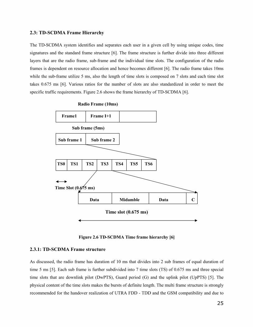
2.3: TD-SCDMA Frame Hierarchy
The TD-SCDMA system identifies and separates each user in a given cell by using unique codes, time
signatures and the standard frame structure [6]. The frame structure is further divide into three different
layers that are the radio frame, sub-frame and the individual time slots. The configuration of the radio
frames is dependent on resource allocation and hence becomes different [6]. The radio frame takes 10ms
while the sub-frame utilize 5 ms, also the length of time slots is composed on 7 slots and each time slot
takes 0.675 ms [6]. Various ratios for the number of slots are also standardized in order to meet the
specific traffic requirements. Figure 2.6 shows the frame hierarchy of TD-SCDMA [6].
Radio Frame (10ms)
Frame1 Frame I+1
Sub frame (5ms)
Sub frame 1 Sub frame 2
TS0 TS1 TS2 TS3 TS4 TS5 TS6
Time Slot (0.675 ms)
Data Midamble Data C
Time slot (0.675 ms)
Figure 2.6 TD-SCDMA Time frame hierarchy [6]
2.3.1: TD-SCDMA Frame structure
As discussed, the radio frame has duration of 10 ms that divides into 2 sub frames of equal duration of
time 5 ms [5]. Each sub frame is further subdivided into 7 time slots (TS) of 0.675 ms and three special
time slots that are downlink pilot (DwPTS), Guard period (G) and the uplink pilot (UpPTS) [5]. The
physical content of the time slots makes the bursts of definite length. The multi frame structure is strongly
recommended for the handover realization of UTRA FDD - TDD and the GSM compatibility and due to
26
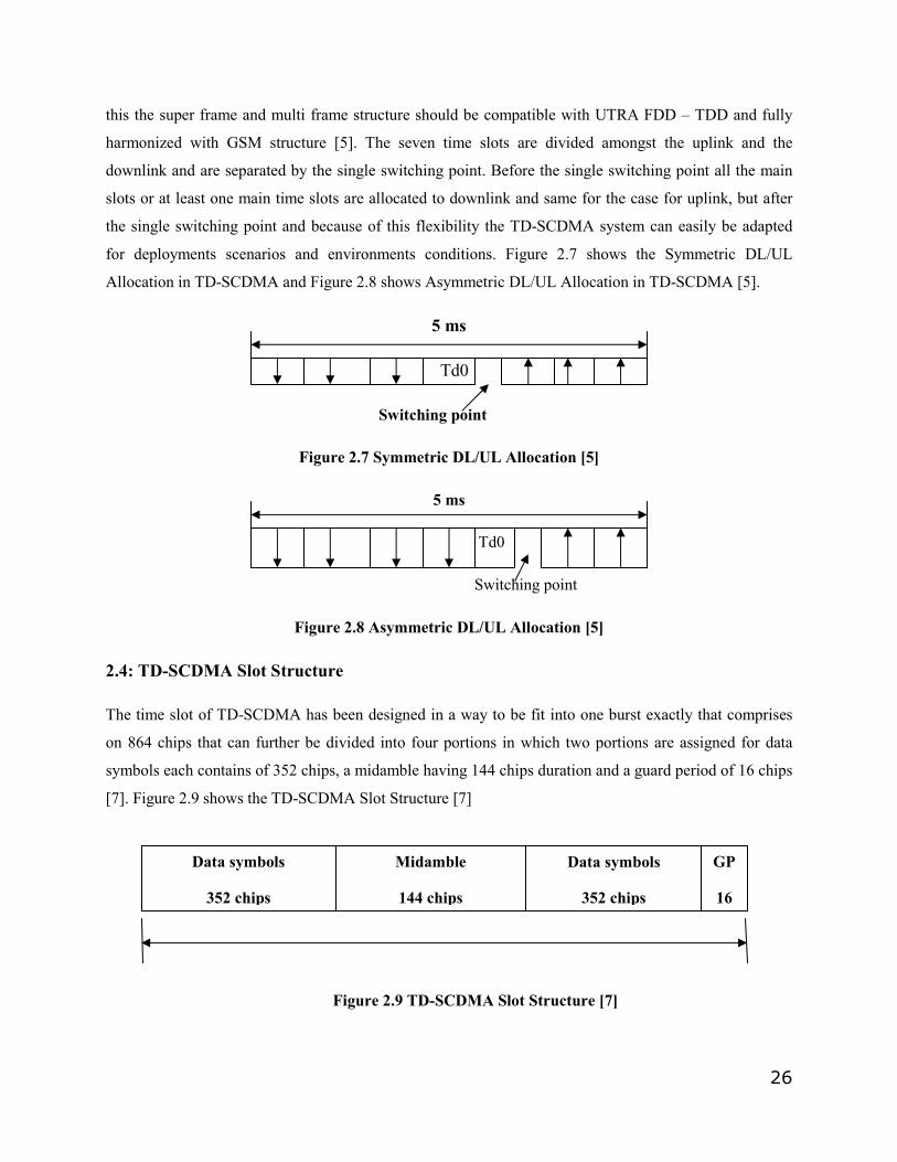
this the super frame and multi frame structure should be compatible with UTRA FDD – TDD and fully
harmonized with GSM structure [5]. The seven time slots are divided amongst the uplink and the
downlink and are separated by the single switching point. Before the single switching point all the main
slots or at least one main time slots are allocated to downlink and same for the case for uplink, but after
the single switching point and because of this flexibility the TD-SCDMA system can easily be adapted
for deployments scenarios and environments conditions. Figure 2.7 shows the Symmetric DL/UL
Allocation in TD-SCDMA and Figure 2.8 shows Asymmetric DL/UL Allocation in TD-SCDMA [5].
5 ms
Td0
Switching point
Figure 2.7 Symmetric DL/UL Allocation [5]
5 ms
Td0
Switching point
Figure 2.8 Asymmetric DL/UL Allocation [5]
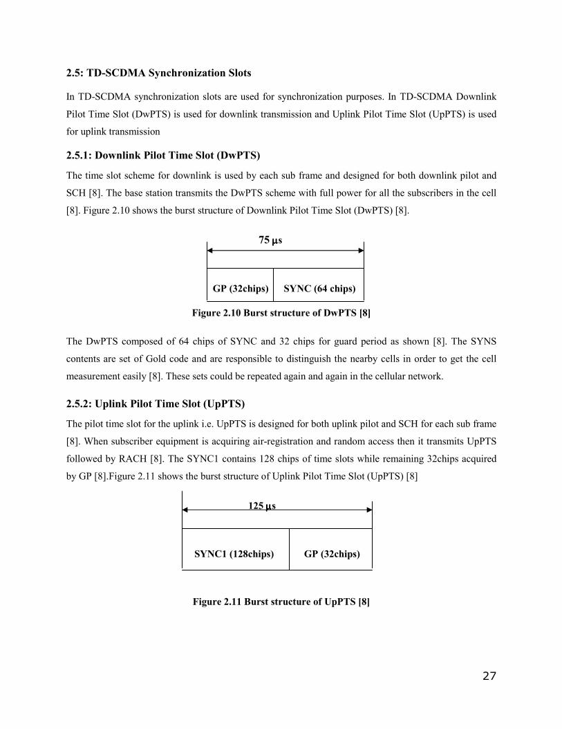
2.4: TD-SCDMA Slot Structure
The time slot of TD-SCDMA has been designed in a way to be fit into one burst exactly that comprises
on 864 chips that can further be divided into four portions in which two portions are assigned for data
symbols each contains of 352 chips, a midamble having 144 chips duration and a guard period of 16 chips
[7]. Figure 2.9 shows the TD-SCDMA Slot Structure [7]
Figure 2.9 TD-SCDMA Slot Structure [7]
Data symbols
352 chips
Midamble
144 chips
Data symbols
352 chips
GP
16
27
2.5: TD-SCDMA Synchronization Slots
In TD-SCDMA synchronization slots are used for synchronization purposes. In TD-SCDMA Downlink
Pilot Time Slot (DwPTS) is used for downlink transmission and Uplink Pilot Time Slot (UpPTS) is used
for uplink transmission
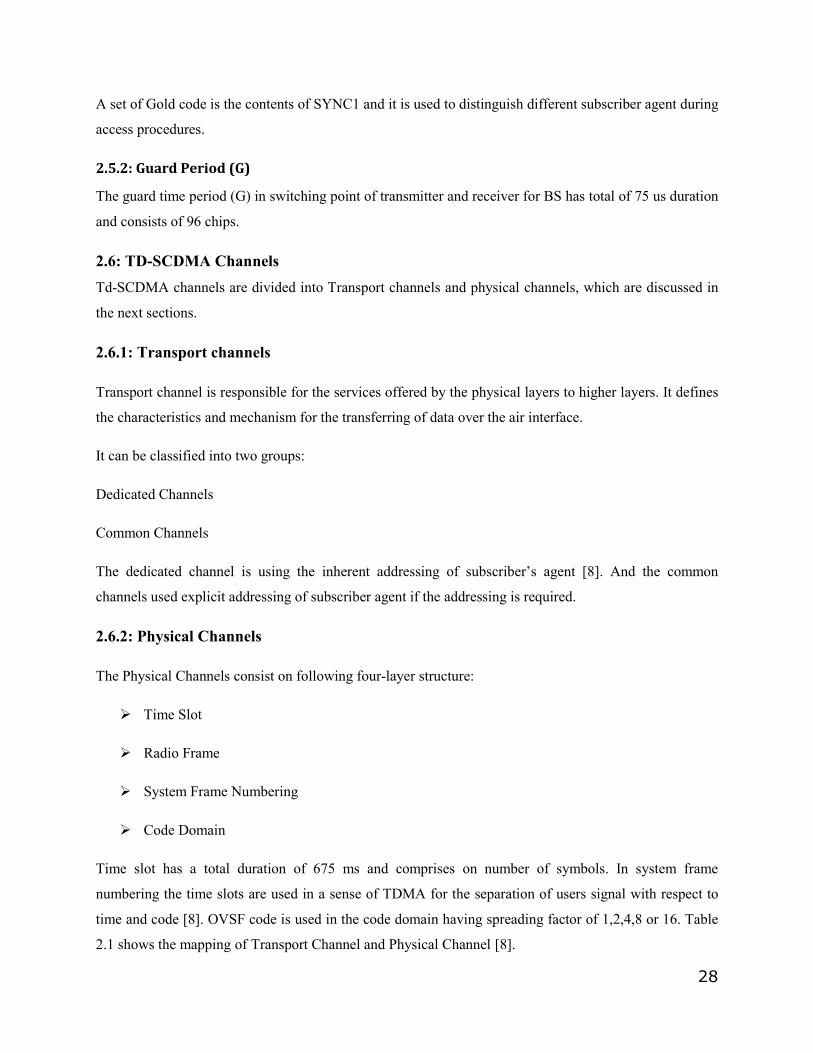
2.5.1: Downlink Pilot Time Slot (DwPTS)
The time slot scheme for downlink is used by each sub frame and designed for both downlink pilot and
SCH [8]. The base station transmits the DwPTS scheme with full power for all the subscribers in the cell
[8]. Figure 2.10 shows the burst structure of Downlink Pilot Time Slot (DwPTS) [8].
75 µµµµs
GP (32chips) SYNC (64 chips)
Figure 2.10 Burst structure of DwPTS [8]
The DwPTS composed of 64 chips of SYNC and 32 chips for guard period as shown [8]. The SYNS
contents are set of Gold code and are responsible to distinguish the nearby cells in order to get the cell
measurement easily [8]. These sets could be repeated again and again in the cellular network.
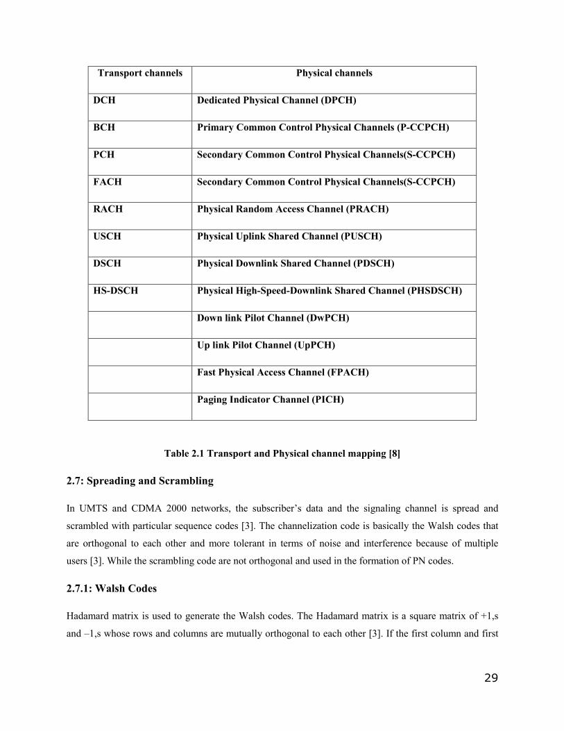
2.5.2: Uplink Pilot Time Slot (UpPTS)
The pilot time slot for the uplink i.e. UpPTS is designed for both uplink pilot and SCH for each sub frame
[8]. When subscriber equipment is acquiring air-registration and random access then it transmits UpPTS
followed by RACH [8]. The SYNC1 contains 128 chips of time slots while remaining 32chips acquired
by GP [8].Figure 2.11 shows the burst structure of Uplink Pilot Time Slot (UpPTS) [8]
125 µµµµs
SYNC1 (128chips) GP (32chips)
Figure 2.11 Burst structure of UpPTS [8]
28
A set of Gold code is the contents of SYNC1 and it is used to distinguish different subscriber agent during
access procedures.
2.5.2: Guard Period (G)
The guard time period (G) in switching point of transmitter and receiver for BS has total of 75 us duration
and consists of 96 chips.
2.6: TD-SCDMA Channels
Td-SCDMA channels are divided into Transport channels and physical channels, which are discussed in
the next sections.
2.6.1: Transport channels
Transport channel is responsible for the services offered by the physical layers to higher layers. It defines
the characteristics and mechanism for the transferring of data over the air interface.
It can be classified into two groups:
Dedicated Channels
Common Channels
The dedicated channel is using the inherent addressing of subscriber’s agent [8]. And the common
channels used explicit addressing of subscriber agent if the addressing is required.
2.6.2: Physical Channels
The Physical Channels consist on following four-layer structure:
Ø Time Slot
Ø Radio Frame
Ø System Frame Numbering
Ø Code Domain
Time slot has a total duration of 675 ms and comprises on number of symbols. In system frame
numbering the time slots are used in a sense of TDMA for the separation of users signal with respect to
time and code [8]. OVSF code is used in the code domain having spreading factor of 1,2,4,8 or 16. Table
2.1 shows the mapping of Transport Channel and Physical Channel [8].
29
Transport channels Physical channels
DCH Dedicated Physical Channel (DPCH)
BCH Primary Common Control Physical Channels (P-CCPCH)
PCH Secondary Common Control Physical Channels(S-CCPCH)
FACH Secondary Common Control Physical Channels(S-CCPCH)
RACH Physical Random Access Channel (PRACH)
USCH Physical Uplink Shared Channel (PUSCH)
DSCH Physical Downlink Shared Channel (PDSCH)
HS-DSCH Physical High-Speed-Downlink Shared Channel (PHSDSCH)
Down link Pilot Channel (DwPCH)
Up link Pilot Channel (UpPCH)
Fast Physical Access Channel (FPACH)
Paging Indicator Channel (PICH)
Table 2.1 Transport and Physical channel mapping [8]
2.7: Spreading and Scrambling
In UMTS and CDMA 2000 networks, the subscriber’s data and the signaling channel is spread and
scrambled with particular sequence codes [3]. The channelization code is basically the Walsh codes that
are orthogonal to each other and more tolerant in terms of noise and interference because of multiple
users [3]. While the scrambling code are not orthogonal and used in the formation of PN codes.
2.7.1: Walsh Codes
Hadamard matrix is used to generate the Walsh codes. The Hadamard matrix is a square matrix of +1,s
and –1,s whose rows and columns are mutually orthogonal to each other [3]. If the first column and first
30
row contain +1 then the matrix is in real form [3]. The +1 is used for binary 1 and -1 is used for binary
0.Figure 2.12 shows the Hadamard matrix of order 2x2 [3].
Figure 2.12 Hadamard matrix of 2x2 order [3]
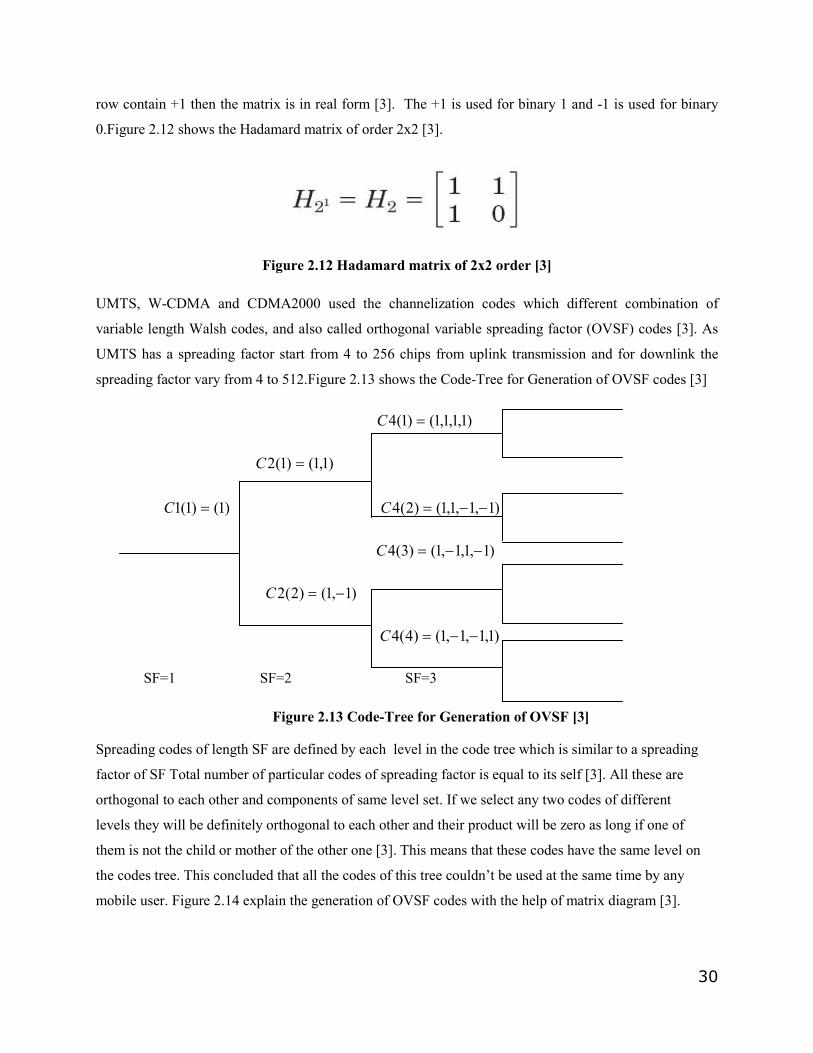
UMTS, W-CDMA and CDMA2000 used the channelization codes which different combination of
variable length Walsh codes, and also called orthogonal variable spreading factor (OVSF) codes [3]. As
UMTS has a spreading factor start from 4 to 256 chips from uplink transmission and for downlink the
spreading factor vary from 4 to 512.Figure 2.13 shows the Code-Tree for Generation of OVSF codes [3]
)1,1,1,1()1(4 =C
)1,1()1(2 =C
)1()1(1 =C )1,1,1,1()2(4 −−=C
)1,1,1,1()3(4 −−=C
)1,1()2(2 −=C
)1,1,1,1()4(4 −−=C
SF=1 SF=2 SF=3
Figure 2.13 Code-Tree for Generation of OVSF [3]
Spreading codes of length SF are defined by each level in the code tree which is similar to a spreading
factor of SF Total number of particular codes of spreading factor is equal to its self [3]. All these are
orthogonal to each other and components of same level set. If we select any two codes of different
levels they will be definitely orthogonal to each other and their product will be zero as long if one of
them is not the child or mother of the other one [3]. This means that these codes have the same level on
the codes tree. This concluded that all the codes of this tree couldn’t be used at the same time by any
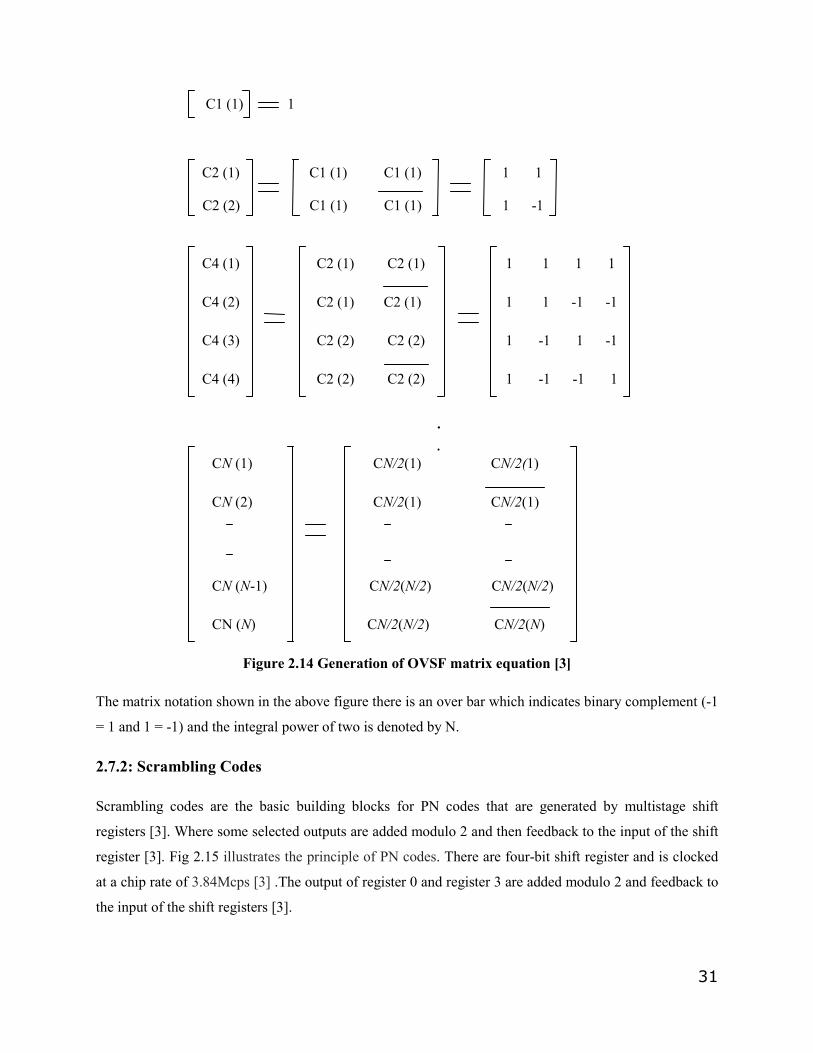
mobile user. Figure 2.14 explain the generation of OVSF codes with the help of matrix diagram [3].
31
C1 (1) 1
C2 (1) C1 (1) C1 (1) 1 1
C2 (2) C1 (1) C1 (1) 1 -1
C4 (1) C2 (1) C2 (1) 1 1 1 1
C4 (2) C2 (1) C2 (1) 1 1 -1 -1
C4 (3) C2 (2) C2 (2) 1 -1 1 -1
C4 (4) C2 (2) C2 (2) 1 -1 -1 1
. . CN (1) CN/2(1) CN/2(1)
CN (2) CN/2(1) CN/2(1)
CN (N-1) CN/2(N/2) CN/2(N/2)
CN (N) CN/2(N/2) CN/2(N)
Figure 2.14 Generation of OVSF matrix equation [3]
The matrix notation shown in the above figure there is an over bar which indicates binary complement (-1
= 1 and 1 = -1) and the integral power of two is denoted by N.
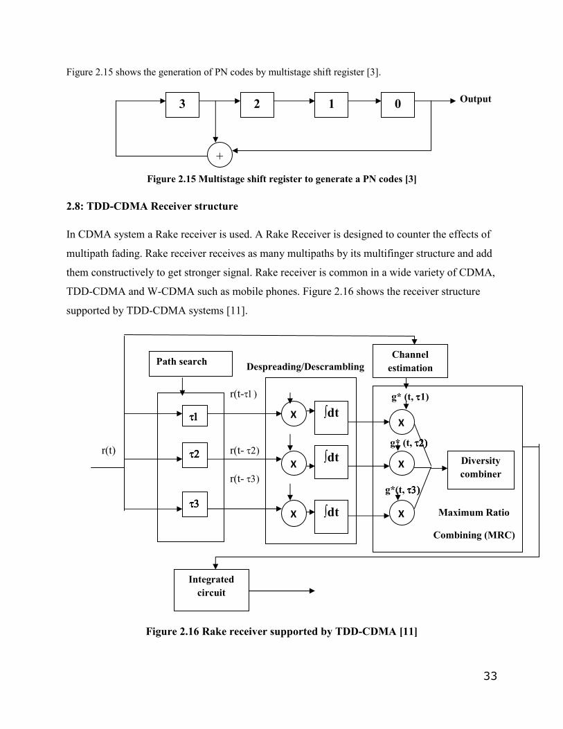
2.7.2: Scrambling Codes
Scrambling codes are the basic building blocks for PN codes that are generated by multistage shift
registers [3]. Where some selected outputs are added modulo 2 and then feedback to the input of the shift
register [3]. Fig 2.15 illustrates the principle of PN codes. There are four-bit shift register and is clocked
at a chip rate of 3.84Mcps [3] .The output of register 0 and register 3 are added modulo 2 and feedback to
the input of the shift registers [3].
32
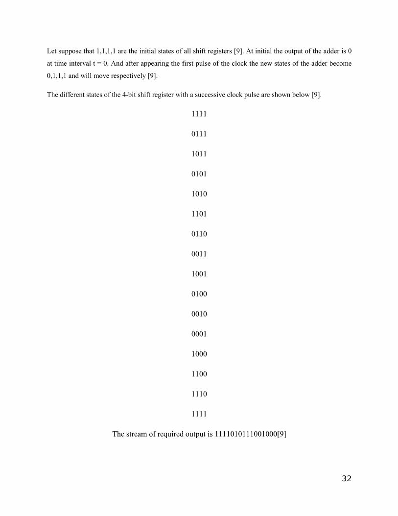
Let suppose that 1,1,1,1 are the initial states of all shift registers [9]. At initial the output of the adder is 0
at time interval t = 0. And after appearing the first pulse of the clock the new states of the adder become
0,1,1,1 and will move respectively [9].
The different states of the 4-bit shift register with a successive clock pulse are shown below [9].
1111
0111
1011
0101
1010
1101
0110
0011
1001
0100
0010
0001
1000
1100
1110
1111
The stream of required output is 1111010111001000[9]
33
Figure 2.15 shows the generation of PN codes by multistage shift register [3].
Output
Figure 2.15 Multistage shift register to generate a PN codes [3]
2.8: TDD-CDMA Receiver structure
In CDMA system a Rake receiver is used. A Rake Receiver is designed to counter the effects of
multipath fading. Rake receiver receives as many multipaths by its multifinger structure and add
them constructively to get stronger signal. Rake receiver is common in a wide variety of CDMA,
TDD-CDMA and W-CDMA such as mobile phones. Figure 2.16 shows the receiver structure
supported by TDD-CDMA systems [11].
Despreading/Descrambling
r(t-τ1)
r(t) r(t- τ2)
r(t- τ3)
Figure 2.16 Rake receiver supported by TDD-CDMA [11]
τ2τ2τ2τ2
τ3τ3τ3τ3
Path search
X
X
X
g* (t, ττττ1)
g* (t, τ2)τ2)τ2)τ2)
g*(t, τ3)τ3)τ3)τ3)
Maximum Ratio
Combining (MRC)
Channel estimation
X
X
X
Diversity combiner
Integrated circuit
τ1τ1τ1τ1 ∫dt
∫dt
∫dt
3 2 1 0
+
34
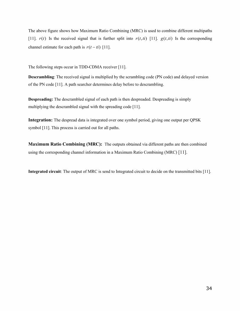
The above figure shows how Maximum Ratio Combining (MRC) is used to combine different multipaths
[11]. )(tr Is the received signal that is further split into ),( titr [11]. ),( titg Is the corresponding
channel estimate for each path is )( titr − [11].
The following steps occur in TDD-CDMA receiver [11]. Descrambling: The received signal is multiplied by the scrambling code (PN code) and delayed version
of the PN code [11]. A path searcher determines delay before to descrambling.
Despreading: The descrambled signal of each path is then despreaded. Despreading is simply
multiplying the descrambled signal with the spreading code [11].
Integration: The despread data is integrated over one symbol period, giving one output per QPSK
symbol [11]. This process is carried out for all paths.
Maximum Ratio Combining (MRC): The outputs obtained via different paths are then combined
using the corresponding channel information in a Maximum Ratio Combining (MRC) [11].
Integrated circuit: The output of MRC is send to Integrated circuit to decide on the transmitted bits [11].
35
Chapter 3: System Model
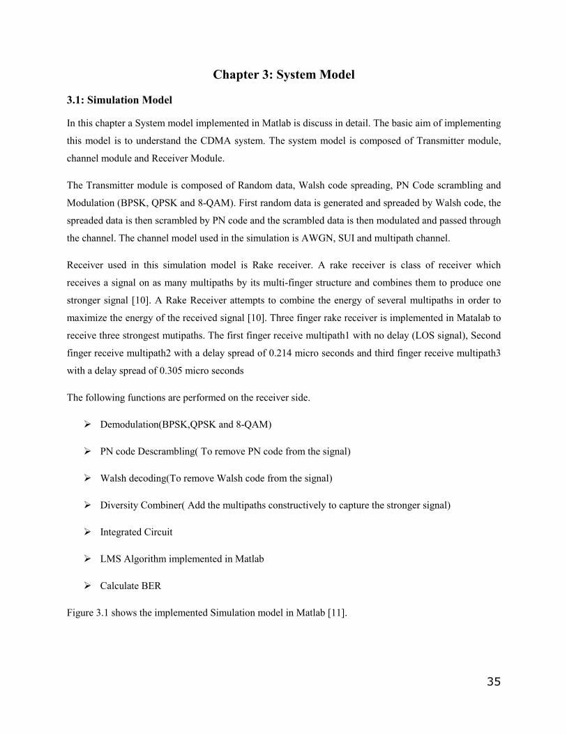
3.1: Simulation Model
In this chapter a System model implemented in Matlab is discuss in detail. The basic aim of implementing
this model is to understand the CDMA system. The system model is composed of Transmitter module,
channel module and Receiver Module.
The Transmitter module is composed of Random data, Walsh code spreading, PN Code scrambling and
Modulation (BPSK, QPSK and 8-QAM). First random data is generated and spreaded by Walsh code, the
spreaded data is then scrambled by PN code and the scrambled data is then modulated and passed through
the channel. The channel model used in the simulation is AWGN, SUI and multipath channel.
Receiver used in this simulation model is Rake receiver. A rake receiver is class of receiver which
receives a signal on as many multipaths by its multi-finger structure and combines them to produce one
stronger signal [10]. A Rake Receiver attempts to combine the energy of several multipaths in order to
maximize the energy of the received signal [10]. Three finger rake receiver is implemented in Matalab to
receive three strongest mutipaths. The first finger receive multipath1 with no delay (LOS signal), Second
finger receive multipath2 with a delay spread of 0.214 micro seconds and third finger receive multipath3
with a delay spread of 0.305 micro seconds
The following functions are performed on the receiver side.
Ø Demodulation(BPSK,QPSK and 8-QAM)
Ø PN code Descrambling( To remove PN code from the signal)
Ø Walsh decoding(To remove Walsh code from the signal)
Ø Diversity Combiner( Add the multipaths constructively to capture the stronger signal)
Ø Integrated Circuit
Ø LMS Algorithm implemented in Matlab
Ø Calculate BER
Figure 3.1 shows the implemented Simulation model in Matlab [11].
36
\
Transmitter
Channel
LOS (M1)
M2 Delay
Dela
M3 Delay
Figure 3.1 Simulation Model [11]
Random data generator
Walsh Code spreading
PN Code scrambling
Modulation (BPSK, QPSK, 8-QAM)
Wireless channel
SUI+AWGN+Multipath
Demodulation (BPSK, QPSK,
8QAM)
PN Descrambling
Walsh Decoding
Demodulation (BPSK, QPSK, 8-
QAM)
PN Descrambling
Walsh Decoding
Diversity Combiner
Integrated Circuit
Demodulation (BPSK, QPSK, 8-
QAM)
PN Descrambling
Walsh Decoding
Calculate BER
Adaptive channel equalization
Training Sequence generation
37
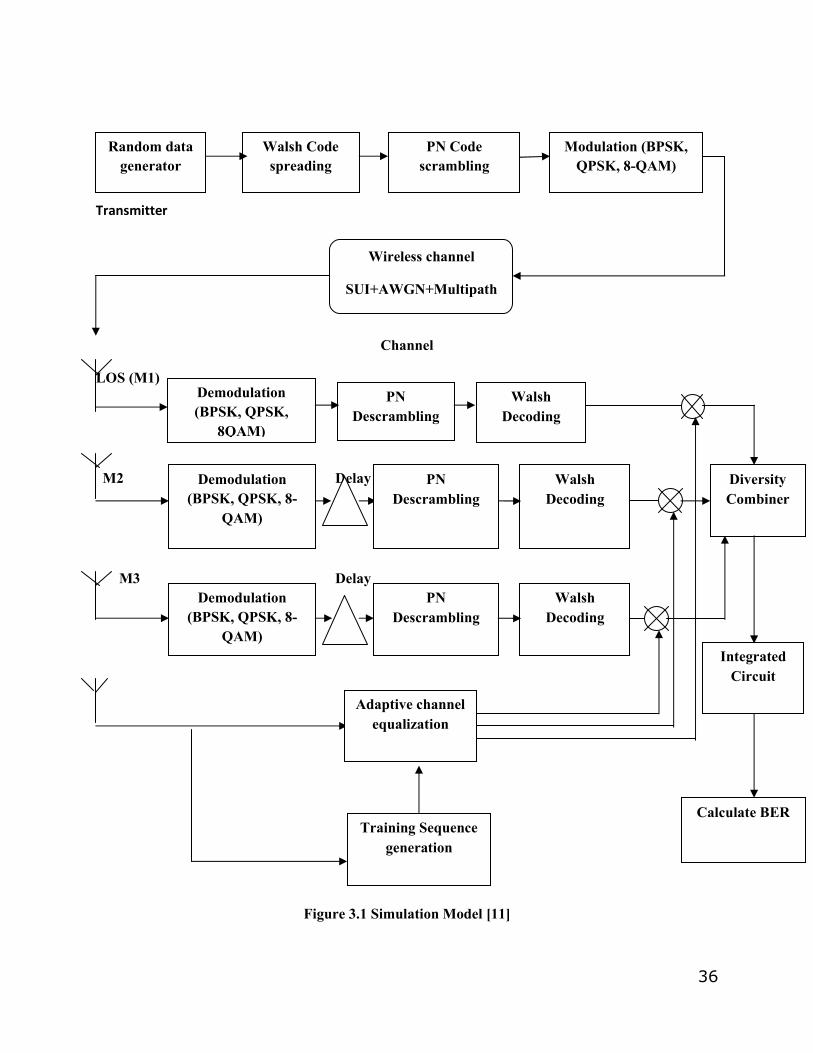
3.2 Transmitter Module
The Transmitter module consists of the following functions.
Ø Random data
Ø Walsh Code spreading ( spread the data by Walsh code)
Ø PN Code scrambling( Scramble the spreaded data by PN code)
Ø Modulation( BPSK, QPSK and 8-QAM)
Figure 3.2 shows the implemented Transmitter module [11].
Figure 3.2.Transmitter Module [11]
3.2.1: Random data generator
It generates the random data of first 100000 bits in the form of 0,s and 1,s and applied as an input to the
transmitter.
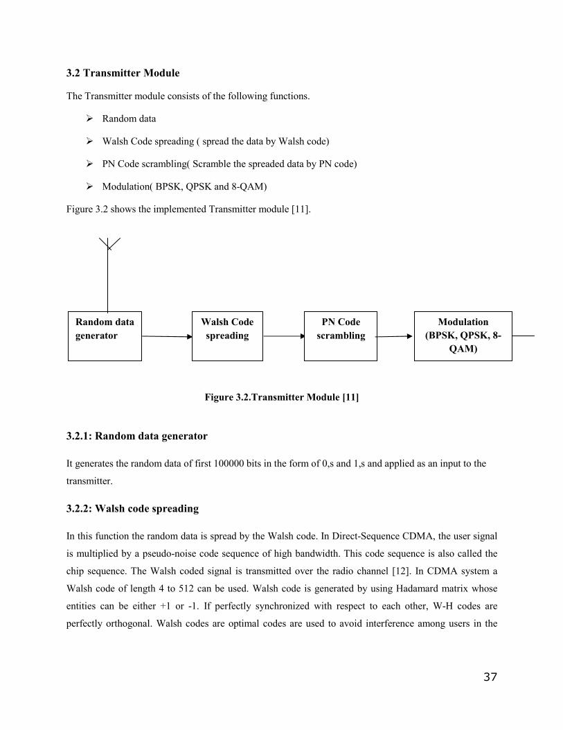
3.2.2: Walsh code spreading
In this function the random data is spread by the Walsh code. In Direct-Sequence CDMA, the user signal
is multiplied by a pseudo-noise code sequence of high bandwidth. This code sequence is also called the
chip sequence. The Walsh coded signal is transmitted over the radio channel [12]. In CDMA system a
Walsh code of length 4 to 512 can be used. Walsh code is generated by using Hadamard matrix whose
entities can be either +1 or -1. If perfectly synchronized with respect to each other, W-H codes are
perfectly orthogonal. Walsh codes are optimal codes are used to avoid interference among users in the
Random data generator
Walsh Code spreading
PN Code scrambling
Modulation (BPSK, QPSK, 8-
QAM)
38
Uplink [12]. Spreading is simply the modulo 2 addition of Walsh code with data. A function is made in
Matlab to spread the data by Walsh code.
3.2.3: PN Code Scrambling
This function scrambles the data by the PN code. Scrambling is simply the process of modulo 2 addition
of the PN code with the data bits [10]. In CDMA system scrambling is used to protect the data from
unauthorized access. In CDMA system every user assigns a specific code called Pseudo Noise (PN) code
[10]. The PN code is generated by the multistage shift register where some selected outputs are added
modulo 2 and then feedback to the input of the shift register [10]. A function is made in matlab, which
generate the PN code; the user may enter the length of the PN code of its own. The function is also
created in matlab that scramble the spreaded data by the PN code.
3.2.4: Digital Modulation
Digital Modulation is the principle of dividing the data streams into several bit streams, each has a much
lower bit rate, and by using these bit streams to modulate several carriers [13]. In digital communication
system the selection of the modulation technique is highly important [13]. The objective of a digital
communication system is to transmit digital data between two or more nodes [13]. This is performed in
real systems with a modulator at the transmitting end and a demodulator at the receiving end [12].
There are three important types of digital modulation, which are as follows:
• Amplitude-Shift Keying (ASK)
• Frequency-Shift Keying (FSK)
• Phase-Shift Keying (PSK)
3.2.4.1: Amplitude-Shift Keying (ASK)
In Amplitude-shift keying (ASK) the phase and frequency of the signal are kept constant while the
amplitude of the signal is continuously changing. ASK modulation represents digital data as a variation in
the amplitude of a carrier wave [14]. In ASK the bit which carries signal 1 is transmitted by some
particular amplitude while in case of transmit 0 the amplitude is kept to be zero.
39
3.2.4.2: Frequency-Shift Keying (FSK)
In Frequency-Shift Keying (FSK) the phase and amplitude of the signal are kept constant while frequency
of the signal is continuously changing. Bit 1 has higher frequency while bit 0 has lower frequency. FSK is
the simplest and most widely used digital modulation scheme. Significant advantages of FSK are very
simple to generate, simple to demodulate and due to the continuously changing of frequency can utilize a
non-linear PA [13]. Significant disadvantages of FSK are poor BER performance and spectral efficiency
[13].
3.2.4.3: Phase-Shift Keying (PSK)
In Phase-Shift Keying (PSK) the frequency and amplitude of the signal are kept constant while phase of
the signal is continuously changing. In FSK the frequency and amplitude of the signal remain constant
while the information of phase change is carried out by sinusoidal carrier. [15].The simplest one of FSK
modulation is Binary phase shift keying (BPSK) [15].
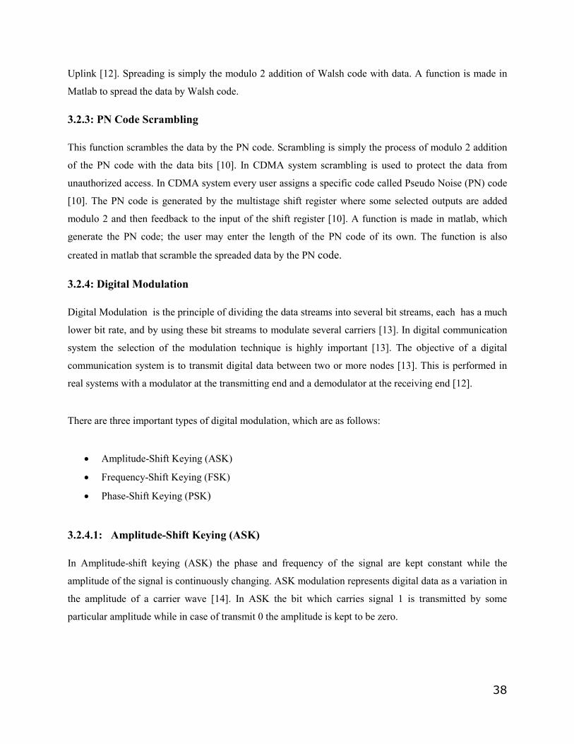
3.3: Binary Phase Shift Keying (BPSK)
The simplest form of phase modulation is binary (two level) phase modulation. With Theoretical BPSK
the carrier phase has only two states, +/- 90 [11]. BPSK reduce the BER of the system. Figure 3.2 shows
the BPSK constellations [16].
Figure 3.3 BPSK constellations [16]
40
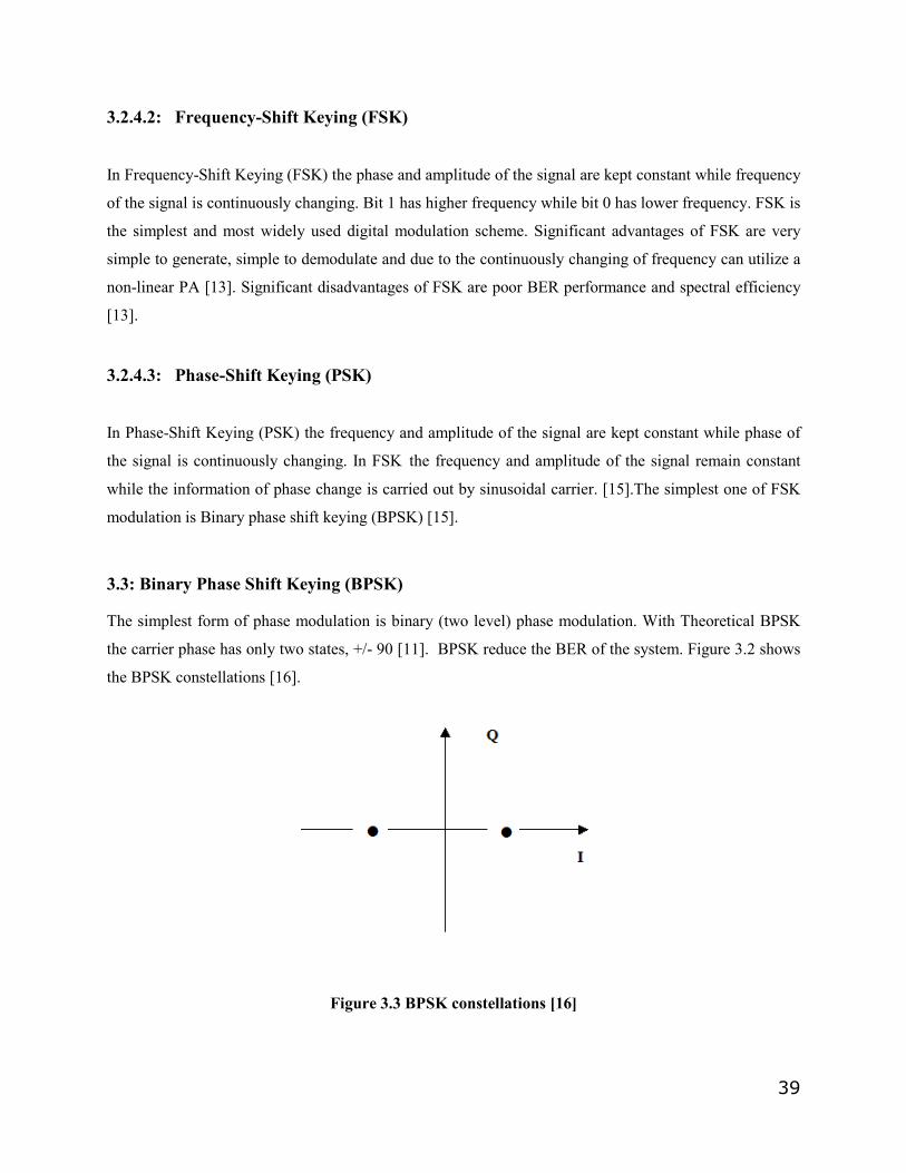
3.4: Quadrature Phase Shift Keying (QPSK)
QPSK modulation is often used in preference to BPSK when higher spectral efficiency is required [13].
QPSK use four constellation points, 0, 90, -90 and 180. Each constellation points representing two bits of
data. QPSK uses more symbols as compared to BPSK. Figure 3.2 shows the QPSK constellations [16].
Figure 3.4 QPSK constellations [16]
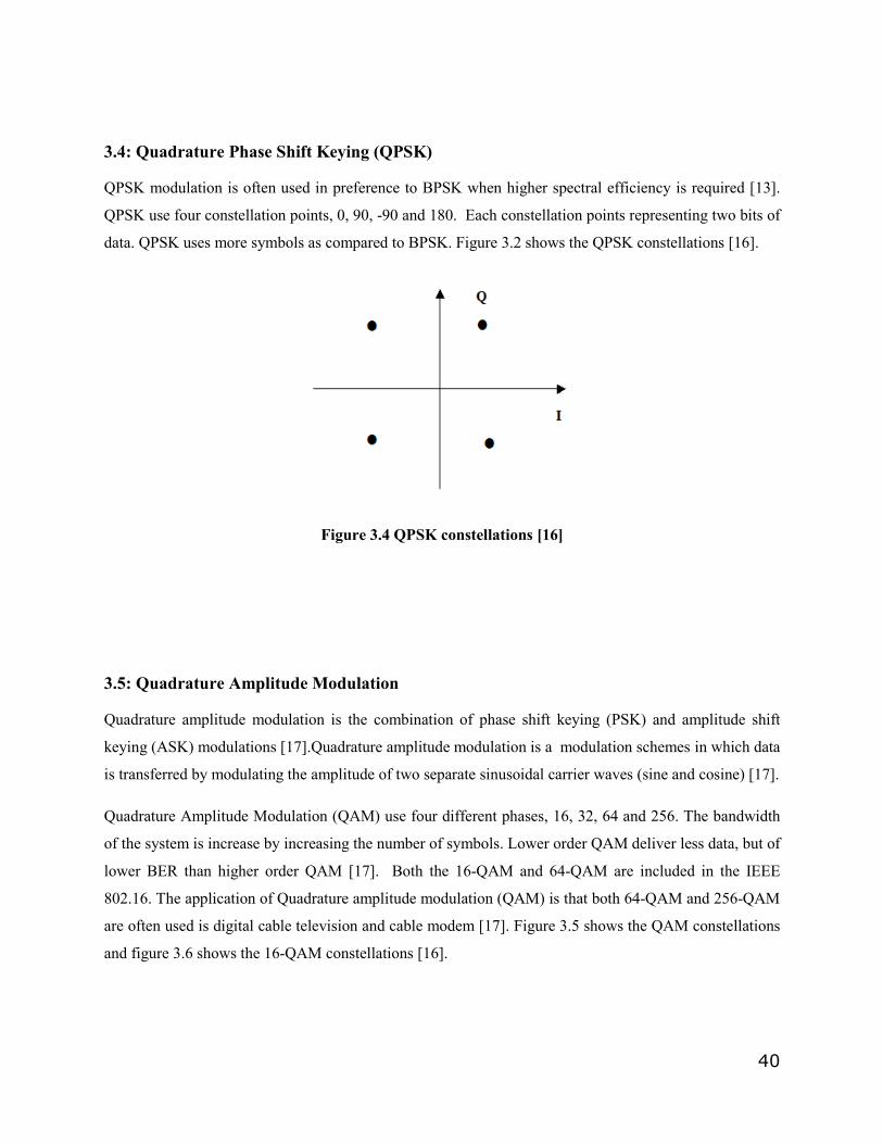
3.5: Quadrature Amplitude Modulation
Quadrature amplitude modulation is the combination of phase shift keying (PSK) and amplitude shift
keying (ASK) modulations [17].Quadrature amplitude modulation is a modulation schemes in which data
is transferred by modulating the amplitude of two separate sinusoidal carrier waves (sine and cosine) [17].
Quadrature Amplitude Modulation (QAM) use four different phases, 16, 32, 64 and 256. The bandwidth
of the system is increase by increasing the number of symbols. Lower order QAM deliver less data, but of
lower BER than higher order QAM [17]. Both the 16-QAM and 64-QAM are included in the IEEE
802.16. The application of Quadrature amplitude modulation (QAM) is that both 64-QAM and 256-QAM
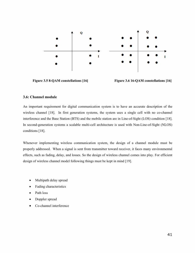
are often used is digital cable television and cable modem [17]. Figure 3.5 shows the QAM constellations
and figure 3.6 shows the 16-QAM constellations [16].
41
Figure 3.5 8-QAM constellations [16] Figure 3.6 16-QAM constellations [16]
3.6: Channel module
An important requirement for digital communication system is to have an accurate description of the
wireless channel [18]. In first generation systems, the system uses a single cell with no co-channel
interference and the Base Station (BTS) and the mobile station are in Line-of-Sight (LOS) condition [18].
In second-generation systems a scalable multi-cell architecture is used with Non-Line-of-Sight (NLOS)
conditions [18].
Whenever implementing wireless communication system, the design of a channel module must be
properly addressed. When a signal is sent from transmitter toward receiver, it faces many environmental
effects, such as fading, delay, and losses. So the design of wireless channel comes into play. For efficient
design of wireless channel model following things must be kept in mind [19].
• Multipath delay spread
• Fading characteristics
• Path loss
• Doppler spread
• Co-channel interference
42
3.6.1: Multipath delay spread
Delay spread is a type of distortion that is caused when an identical signal arrives at receiver with
different time interval [20]. The time difference between the arrival time of the first multipath component
and the last multipath component is called delay spread [20]. The multipath signal usually arrives with
different angle of arrival at receiver. Due to the non line of sight propagation nature of the TD-SCDMA,
multipath delay spread is address in the channel model.
3.6.2: Fading characteristics
In communication system a fading channel is a channel that experience a fading [19]. In wireless
communication systems, fading may be either due to multipath propagation or due to shadowing from
obstacles [19]. Due to fading the receiver receives multiple copies of the transmitted signal, each arriving
at different path [19]. Each signal copy will experience a change in delay, attenuation and phase shift
while traveling form the transmitter to the receiver [19]. This can produce either constructive or
destructive interference .Small scale fading has also been considered in the channel. When there is NLSO
signal component and multiple reflective paths are large in number then Rayleigh fading calls small scale
fading. When there is LOS signal component along with the multiple reflective paths then a Rician fading
calls small scale fading.
3.6.3: Path loss
Path loss is commonly used in wireless communication systems and signal propagation [21]. In
telecommunication systems path loss is a major component in the analysis and design of the link budget
[21]. Path loss may occur due to many effects, such as free-space loss, reflection, refraction, difraction
and absorption [21].
3.6.4: Doppler spread
Doppler spread basically occurs due to the relative motion of object or due to the movement of the
communication devices in the environment. The coherence time (Tc) and Doppler spread (Bd) are
inversely proportional to each other [22]. If the bandwidth of Doppler spread (Bd) is much less than the
bandwidth of baseband signal then the effect of Doppler spread is negligible [22].
43
3.6.5: Co-channel interference
Co-channel interference is one the main problem faced by the engineers deal during wireless
communication system. Co-channel interference occurs when the same frequency from two different
mobile stations reaches the same receive. Thus the receiver has the problem to determine that the signal
comes from which user. Figure 3.7 shows the Scenario of Co-channel Interference [23].
Figure 3.7: Co-channel Interference Scenario [23]
There are several causes of co-channel interference, such as poor frequency planning, overly crowded
radio spectrum and adverse weather conditions. To solve the problem of Co-channel interference smart
antennas are used. Smart antennas provide strong resistance against co-channel interference by throwing
NULL towards unwanted users and directing a beam towards the desired user [23].
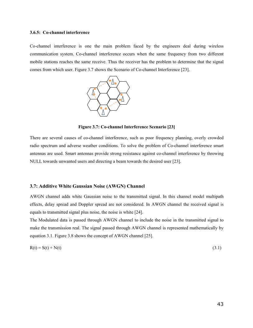
3.7: Additive White Gaussian Noise (AWGN) Channel
AWGN channel adds white Gaussian noise to the transmitted signal. In this channel model multipath
effects, delay spread and Doppler spread are not considered. In AWGN channel the received signal is
equals to transmitted signal plus noise, the noise is white [24].
The Modulated data is passed through AWGN channel to include the noise in the transmitted signal to
make the transmission real. The signal passed through AWGN channel is represented mathematically by
equation 3.1. Figure 3.8 shows the concept of AWGN channel [25].
R(t) = S(t) + N(t) (3.1)
44
Transmitted Signal S (t) Received Signal R(t)
Noise N (t)
Figure 3.8.AWGN Channel [25]
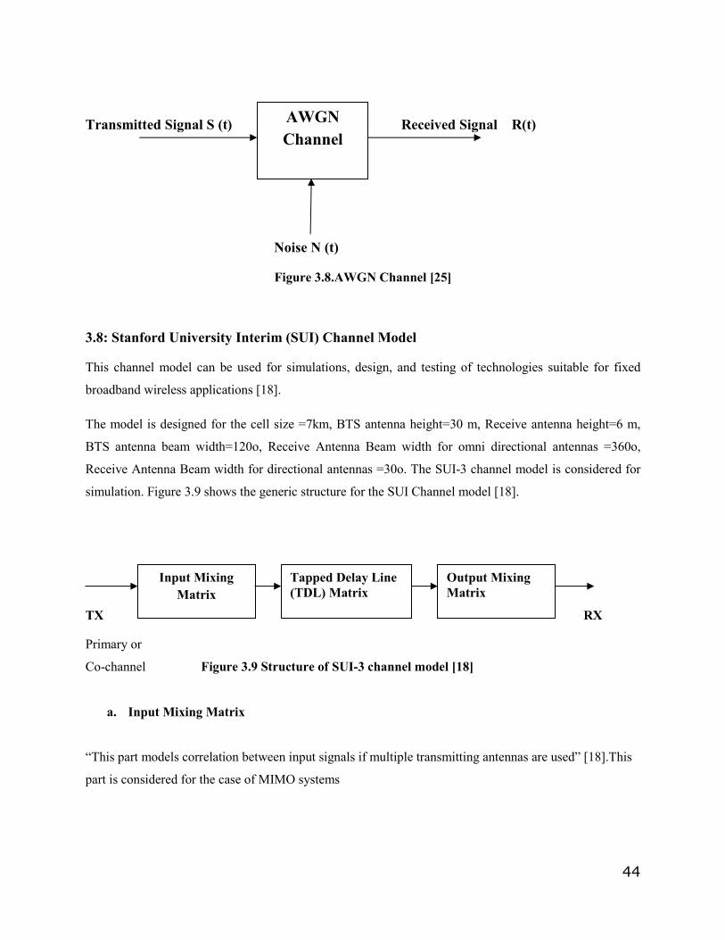
3.8: Stanford University Interim (SUI) Channel Model
This channel model can be used for simulations, design, and testing of technologies suitable for fixed
broadband wireless applications [18].
The model is designed for the cell size =7km, BTS antenna height=30 m, Receive antenna height=6 m,
BTS antenna beam width=120o, Receive Antenna Beam width for omni directional antennas =360o,
Receive Antenna Beam width for directional antennas =30o. The SUI-3 channel model is considered for
simulation. Figure 3.9 shows the generic structure for the SUI Channel model [18].
TX RX
Primary or
Co-channel Figure 3.9 Structure of SUI-3 channel model [18]
a. Input Mixing Matrix
“This part models correlation between input signals if multiple transmitting antennas are used” [18].This
part is considered for the case of MIMO systems
AWGN Channel
Input Mixing Matrix
Tapped Delay Line (TDL) Matrix
Output Mixing Matrix
45
b. Tapped Delay Line (TDL) Matrix
This part modeled the multipath fading of the channel [18]. “The multipath fading is modeled as a
Tapped-delay line with 3 taps with non-uniform delays” [18]. “The gain associated with each tap is
characterized by a distribution (Ricean with a K-factor > 0, or Rayleigh with K-factor = 0) and the
maximum Doppler frequency” [18].
c. Output Mixing Matrix
“This part models the correlation between output signals if multiple receiving antennas are used” [18].
This part is considered for the case of SIMO and MIMO.
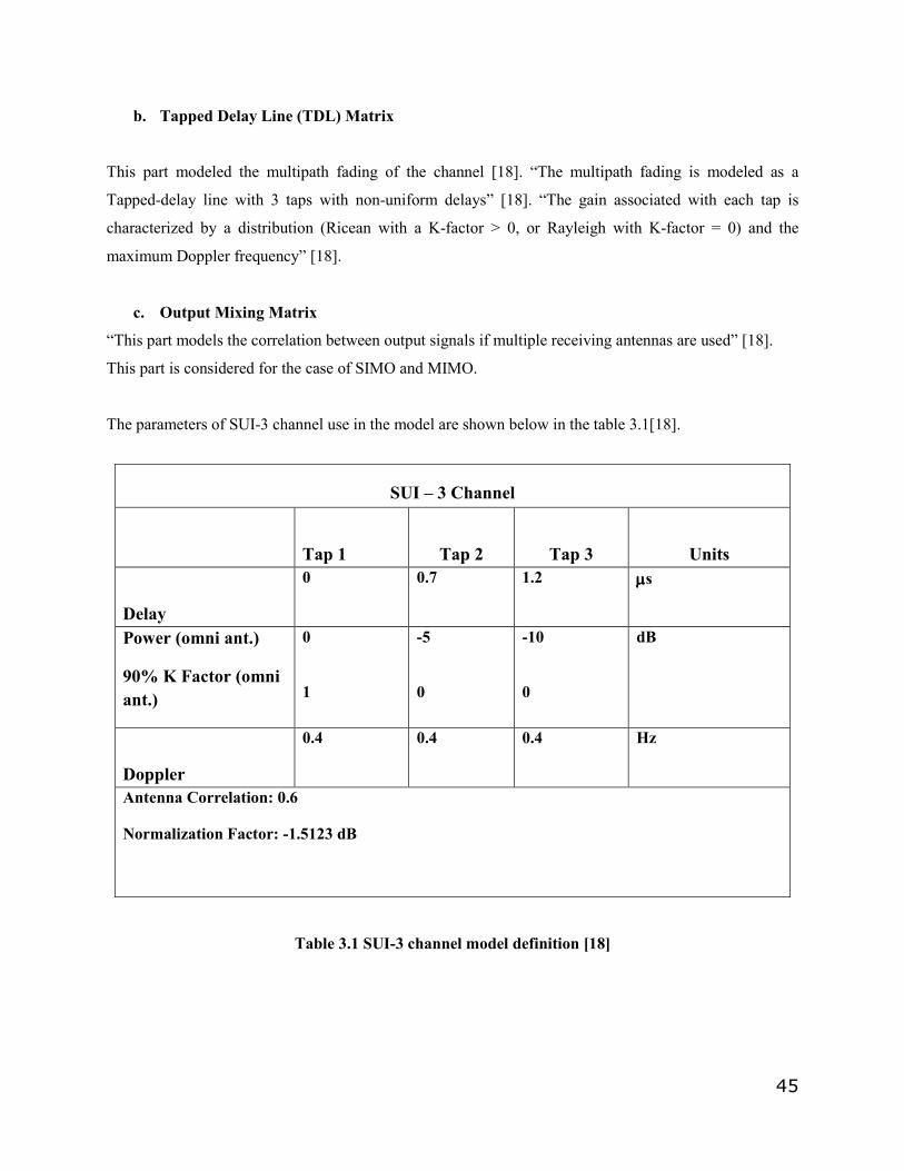
The parameters of SUI-3 channel use in the model are shown below in the table 3.1[18].
Table 3.1 SUI-3 channel model definition [18]
SUI – 3 Channel
Tap 1 Tap 2 Tap 3 Units
Delay
0 0.7 1.2 µµµµs
Power (omni ant.)
90% K Factor (omni ant.)
0
1
-5
0
-10
0
dB
Doppler
0.4 0.4 0.4 Hz
Antenna Correlation: 0.6
Normalization Factor: -1.5123 dB
46
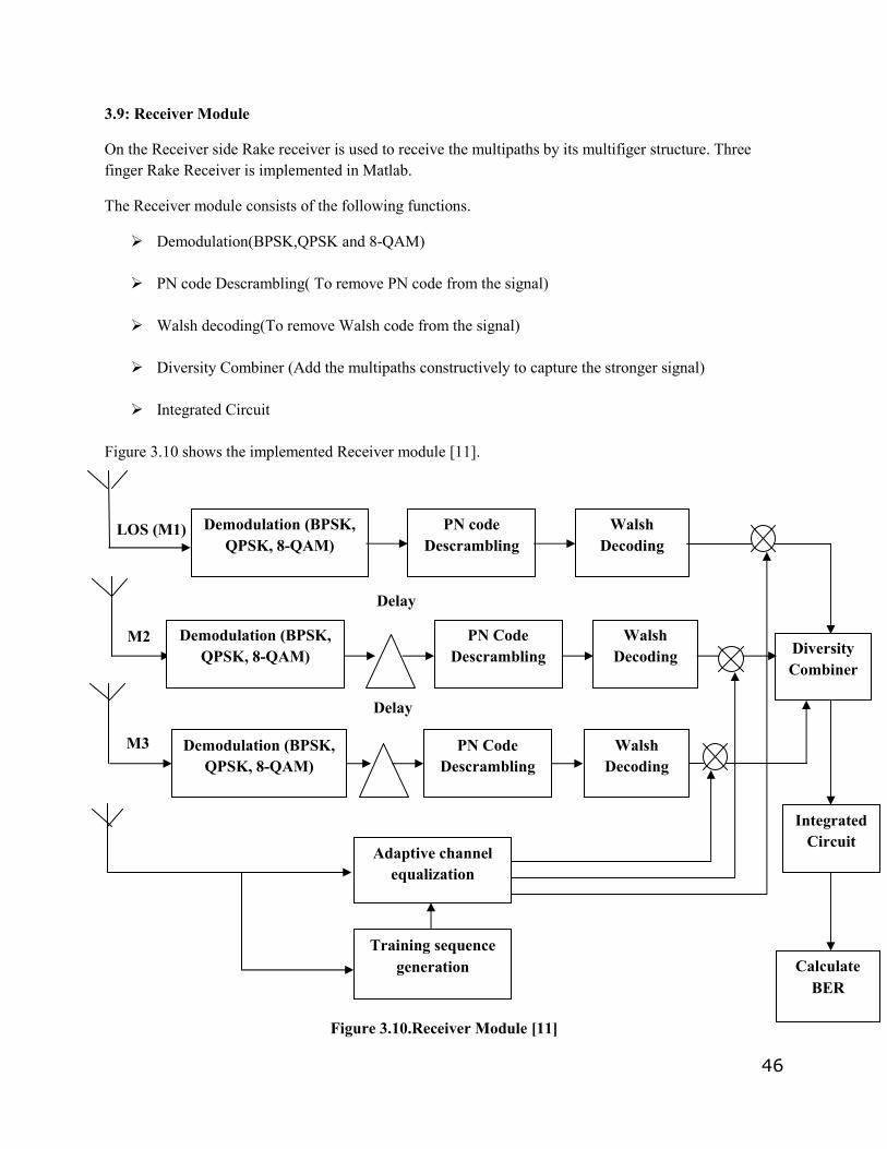
3.9: Receiver Module
On the Receiver side Rake receiver is used to receive the multipaths by its multifiger structure. Three finger Rake Receiver is implemented in Matlab.
The Receiver module consists of the following functions.
Ø Demodulation(BPSK,QPSK and 8-QAM)
Ø PN code Descrambling( To remove PN code from the signal)
Ø Walsh decoding(To remove Walsh code from the signal)
Ø Diversity Combiner (Add the multipaths constructively to capture the stronger signal)
Ø Integrated Circuit
Figure 3.10 shows the implemented Receiver module [11].
LOS (M1)
Delay
M2
Delay
M3
Figure 3.10.Receiver Module [11]
Demodulation (BPSK, QPSK, 8-QAM)
PN code Descrambling
Walsh Decoding
Demodulation (BPSK, QPSK, 8-QAM)
PN Code Descrambling
Walsh Decoding
Integrated Circuit
Diversity Combiner
Calculate BER
Demodulation (BPSK, QPSK, 8-QAM)
PN Code Descrambling
Walsh Decoding
Adaptive channel equalization
Training sequence generation
47
3.9.1: Demodulation (BPSK, QPSK, 8-QAM)
In Demodulation, information is taken out from a modulated carrier [26]. There are several demodulation
schemes but BPSK, QPSK, 8-QAM are used in the simulation.
3.9.2: PN Code Descrambling.
This function descrambles the demodulated data by the PN code, which is the same as used in the
transmitter. Descrambling process is simply the XOR operation of the PN code with the Demodulated
data [10].
3.9.3: Walsh decoding.
This process simply removes the Walsh code from the data. It is simply the XOR operation of the Walsh
code with the descrambled data [10]. The Walsh code will be the same as used in the transmitter.
3.9.4: Adaptive Channel equalization
Adaptive channel estimation is used to compensate for signal distortion in communication channel.
Adaptive channel equalization use adaptive filters to estimate the channel [27]. When the transmitted
signal is passed through the channel, the signal that contains information might become distorted. To
compensate the transmitted signal distortion, adaptive filter can apply to the communication channel [27].
Adaptive filter work as adaptive channel estimation. The adaptive channel equalization is implemented on
the receiver side to reduce the BER of the system.
In this system we have two modes of operations.
1) Rake receiver with perfect channel estimations:
2) Rake receiver with non-perfect channel estimations.
First the performance of Rake receiver is checked with perfect channel estimations using LMS algorithm
and then for non –perfect channel estimations using with out LMS algorithm.
3.9.5: Diversity Combiner
The receiver used in the system is rake receiver and one of the advantages of rake receiver is diversity
combiner. Through diversity combiner it receives the data by its multifinger structure and add them
constructively [10] .In the simulation we used diversity combiner, the output of channel equalization
algorithm is passed through Multipath1, Multipath 2, Multipath3 and add then constructively and send it
to decision threshold.
48
3.9.6: Integrated Circuit and Decision Threshold
The output of the diversity combiner is then added to an integrator circuit the integrator adds up the signal
power over one bit interval Tb of the base band message (Spreading factor) [10]. The output of the
integrator is applied to decision threshold, which takes decision based on the output of the integrator,
whether or not the particular bit is a 0 or 1 [10]. If the output of the integrator is greater than 0, then the
decision is 1, if the output of the integrator is less than 0, then the decision is 0.
49
Chapter 4: Channel estimation Algorithms
4.1: Channel Estimation
Channel estimation algorithms are applied on the receiver side. The signal is passing through the channel
and is received by the channel estimator algorithms. The receiving signal is not in the original shape.
During transmission the signal is affected by many kinds of noises and fading effects. Since the channel
estimation algorithm estimate the channel parameter with help of the training sequence and then this
information is used in the receiver to extract the original data. The main advantages of these algorithms
are that it gives us efficient data from a mixture of different kind of signal and noise etc. These algorithms
reduce the error noise ratio and also probability of errors.
In Telecommunication the radio channel often consists of multipath fading channels. This will cause
intersymbol interference (ISI) in the received signal. To remove the ISI, many kind channel equalizers are
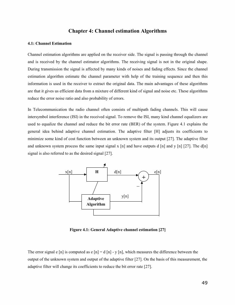
used to equalize the channel and reduce the bit error rate (BER) of the system. Figure 4.1 explains the
general idea behind adaptive channel estimation. The adaptive filter [H] adjusts its coefficients to
minimize some kind of cost function between an unknown system and its output [27]. The adaptive filter
and unknown system process the same input signal x [n] and have outputs d [n] and y [n] [27]. The d[n]
signal is also referred to as the desired signal [27].
x[n] d[n] e[n]
_
y[n]
Figure 4.1: General Adaptive channel estimation [27]
The error signal e [n] is computed as e [n] = d [n] - y [n], which measures the difference between the
output of the unknown system and output of the adaptive filter [27]. On the basis of this measurement, the
adaptive filter will change its coefficients to reduce the bit error rate [27].
H
Adaptive Algorithm
+
50
The most popular channel estimation algorithms will be discussed in the following sections.
4.2: Optimal Adaptive Maximum Likelihood Sequence Estimation (MLSE) Algorithm
The Adaptive MLSE Algorithm is also used for channel Estimation. The MLSE is the optimum receiver
in the presence of intersymbol interference (ISI) gives estimation of the channel impulse response [27].
An MLSE receiver uses a trellis diagram with the veterbi algorithms to obtain maximum estimates of the
symbols. MLSE equalizer is usually adopted to reduce the Bit Error Rate (BER) of the system [27].
MLSE Equalizer estimates the symbol sequence by using veterbi algorithm, so often called viterbi in
European cellular systems [27]. It cancels the intersymbol interference (ISI) linearly [27]. Its complexity
increase with the increase in length of impulse response [27]. The MLSE algorithm is very complex as
compared to other channel estimation algorithms like MMSE and is also higher cast as compared to
MMSE.
4.3: Adaptive Minimum Mean Square Error (MMSE) Algorithm
The Minimum Mean Square Error (MMSE) algorithm has received great attention in the last years as the
optimum linear solution for reducing the Multiple Access Interference (MAI) in DS-CDMA systems [27].
To achieve the best error rate of the system MMSE algorithm is good than all channel estimation
algorithms. The main advantage of MMSE Algorithm is that it is very easy implementation and low
complex structure [27]. There are two main classes of MMSE algorithm.
4.3.1: Optimal MMSE Receiver
The optimal MMSE receiver, which requires the knowledge of the Instantaneous power profile for all
users [27]. In practice the instantaneous power profile is difficult to obtain [27]. Optimal MMSE receiver
produce best Symbol error rate (SIR) result among all others channel estimation receivers.
4.3.2: Sub optimal MMSE Receiver
The sub optimal MMSE receiver, which treats the equal instantaneous powers of all the users [27]. In
practical communication system sub optimal MMSE receiver is of great importance [27]. But in case of
Bit error rate (BER) of the system sub optimal MMSE receiver has not good result as compared to
Optimal MMSE Receiver [27].
4.3.2.1 The Least Mean Squares (LMS) Algorithm
This algorithm was developed by Stanford University professor Bernard Window and Ph.D. student; Ted
Hoff in 1960. LMS is an adaptive algorithm, which uses a gradient-based method of steepest decent [28].
51
From the available data LMS algorithm uses the estimates of the gradient vector [28]. LMS algorithm
uses an iterative procedure that makes corrections to the weight vector in the direction of the negative of
the gradient vector which minimizes the mean square error [28]. LMS does not require matrix inversions
nor does it require correlation function calculation [28]. LMS is the most popular channel estimation
algorithm. LMS has been widely used in the modern communication technology because of its easy
implementation and low complexity. LMS algorithms are used in adaptive filters to find the filter
coefficients to producing the least mean squares of the error signal. The LMS algorithm provides the good
result if the speed of channel change is slow.
There are several types of the LMS algorithm [28]. The Normalized LMS (NLMS) and the Newton LMS
[28]. The Normalized LMS (NLMS) improves the convergence speed in a non-static environment [28]. In
Newton LMS, the weight update equation includes whitening in order to achieve a single mode of
convergence [28]. To make LMS faster Block LMS is used [28]. The input signal is divided into blocks
and weights are updated block wise in block LMS [28]. Sign LMS is called the simple version of LMS
[28]. Sign LMS uses the sign of the error to update the weights [28]. LMS is not a blind algorithm; it
requires a priori information for the reference signal [28].
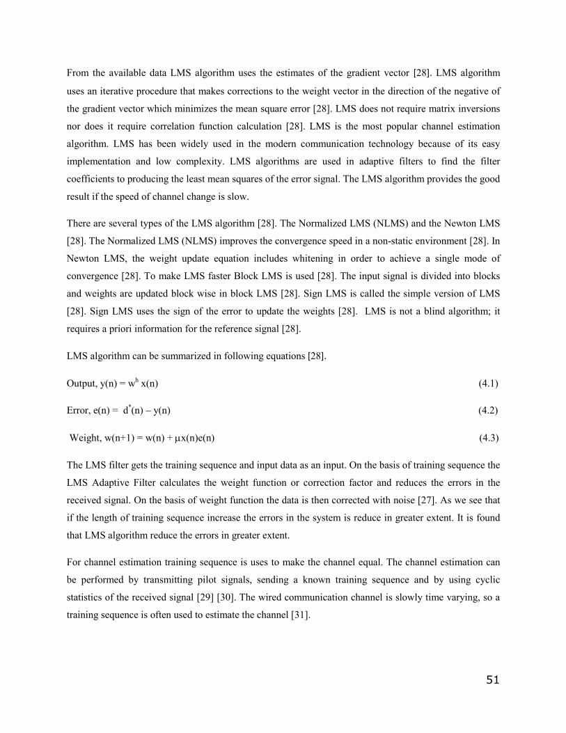
LMS algorithm can be summarized in following equations [28].
Output, y(n) = wh x(n) (4.1)
Error, e(n) = d*(n) – y(n) (4.2)
Weight, w(n+1) = w(n) + µx(n)e(n) (4.3)
The LMS filter gets the training sequence and input data as an input. On the basis of training sequence the
LMS Adaptive Filter calculates the weight function or correction factor and reduces the errors in the
received signal. On the basis of weight function the data is then corrected with noise [27]. As we see that
if the length of training sequence increase the errors in the system is reduce in greater extent. It is found
that LMS algorithm reduce the errors in greater extent.
For channel estimation training sequence is uses to make the channel equal. The channel estimation can
be performed by transmitting pilot signals, sending a known training sequence and by using cyclic
statistics of the received signal [29] [30]. The wired communication channel is slowly time varying, so a
training sequence is often used to estimate the channel [31].
52
4.3.2.2 The Recursive Least squares (RLS) Algorithm
The rate of convergence of RLS algorithm is much faster than the LMS algorithm, because the RLS
algorithm utilizes all the information contained in the input data from the start of the adaptation process
[32]. RLS algorithm is also used for channel estimation, but is not so popular like LMS because of its
difficult Implementation and complex structure. RLS algorithm is used in adaptive filters to find the filter
coefficients that relate to recursively producing the least squares of the error signal. RLS works different
to other channel estimation algorithms to reduce the mean square error.
In the LMS algorithm, the correction that is applied in updating the old estimate of the coefficient vector
is based on the error signal and instantaneous sample value of the tap-input vector [32]. In RLS algorithm
the computation of this correction utilizes all the past available information [32].
In the LMS algorithms, the correction applied to the previous estimate consists of the product of three
factors i.e. the error signal e (n-1), the (scalar) step-size parameter µ, and the tap-input vector u(n-1) [32].
On the other hand, in the RLS algorithm this correction consists of the product of two factors i.e. the gain
vector k (n) and the true estimation error η(n) [32]. The gain vector itself consists of Φ-1(n), the tap-input
vector u (n) multiplied by the inverse of the deterministic correlation matrix [32]. The major difference
between the RLS and LMS algorithms is the presence of Φ-1(n) in the correction term of the RLS
algorithm that has the effect of decorrelating the successive tap inputs, thereby making the RLS a self-
orthogonalizing [32]. Due to this property, RLS algorithm is independent of the eigenvalue spread of the
correlation matrix of the filter input [32].
4.4 Choice of Algorithm
LMS algorithm is chosen in this thesis because it’s a good compromise between performance and
complexity. LMS algorithm is used widely in modern communication technology due to its less complex
structure and simple implementation. LMS algorithm has Stable and robust performance against different
signal conditions. LMS algorithm has mean square error (MSE) behavior.
53
Chapter 5: Simulation Results 5.1: Simulation Environment In this chapter the Simulation results is presented. The presented simulation results are implemented in
Matlab. First the performance of the system is checked for SISO case by using AWGN channel and then
SUI channel [15]. The SUI channel has worst performance due to multipath, delay spread and Doppler
effects. To reduce the BER in SUI channel adaptive LMS algorithm is implemented on receiver side.
Secondly the performance of the system is checked for SIMO case by using Optimal and Sub Optimal
receiver The Rake receiver is Optimal when it has perfect knowledge about the time delays, Doppler
spread and multipaths effects on the channel. The Rake receiver is Sub Optimal when we estimate these
parameters with LMS algorithm.
The receiver used in the system is Rake receiver. A rake receiver is class of receiver implemented in
CDMA handsets, receives a signal on as many multipaths by its multi-finger structure and combines them
to produce one stronger signal [10]. A Rake Receiver attempts to combine the energy of several
multipaths in order to maximize the energy of the received signal [10].
The basic principle of RAKE receiver is simply a multi-finger structure to capture the various multi-
paths [10]. The RAKE receiver tries to listen to the strongest of these multi-paths and then combines
them constructively to get higher signal strength and thus improves bit error rate (BER) [10]. In
wireless environments, the delay between multi-path components is usually large and, if the chip rate is
commonly selected, the low auto-correlation properties of a CDMA spreading sequence can assure that
multi-path components will appear nearly un-correlated with each other [10].
Our simulated rake receiver consists of three fingers that are capable of receiving three multipaths.
The multipaths arriving at the receiver are predetermined as:
Ø First multipath (m1) is arriving with no delay (LOS).
Ø Second multipath (m2) is arriving at a delay spread of 0.214 micro seconds.
Ø Third multipath (m3) is arriving at a delay spread of 0.305 micro seconds.
Assume that three Correlators are used in CDMA Rake receiver to capture the three strongest
multipaths. Correlator1 is synchronized to the strongest multipath (m1). The second correlator is
synchronized to m2; it correlates strongly with m2 but has low correlation with m1. The other correlator
similarly works on the same principle.
54
Monte Carlo simulation was used to test the whole system. The objective of the Monte Carlo simulation
is to estimate the Bit error rate (BER) our system can achieve [33]. In Monte Carlo simulation, the
system is simulated repeatedly, for each simulation count the number of transmitted symbol and symbol
errors, estimate the symbol error rate as the ratio of the total number of observed errors and the total
number of transmitted bits [33]. Let us consider the SISO case by using BPSK modulation and SUI is a
channel. The simulation is repeated 100 times, for each simulation the BER is calculated and later the
average BER is calculated and ploted verses Eb/No, same for the whole system.
The simulation consist of the following steps
Ø Random Data.
Ø Spreading of data by Walsh Code
Ø Scrambling of data by PN Code
Ø Modulation schemes i.e. BPSK, QPKS, and 8-QAM.
Ø Channel Type i.e. AWGN, SUI-3and multipath
Ø Demodulation schemes i.e. BPSK,QPSK and 8-QAM
Ø Descrambling of data
Ø Despreading of data.
Ø Implementation of Adaptive LMS algorithm on Receiver side.
Ø Entire simulation is checked with AWGN channel.
Ø Entire simulation is checked with AWGN and SUI-3.
Ø Entire simulation is checked for Optimal and Sub optimal Receiver
55
5.2: SISO (Single Input Single Output)
In this section, the simulation results are shown when a single antenna at both transmitter and receiver are
used.
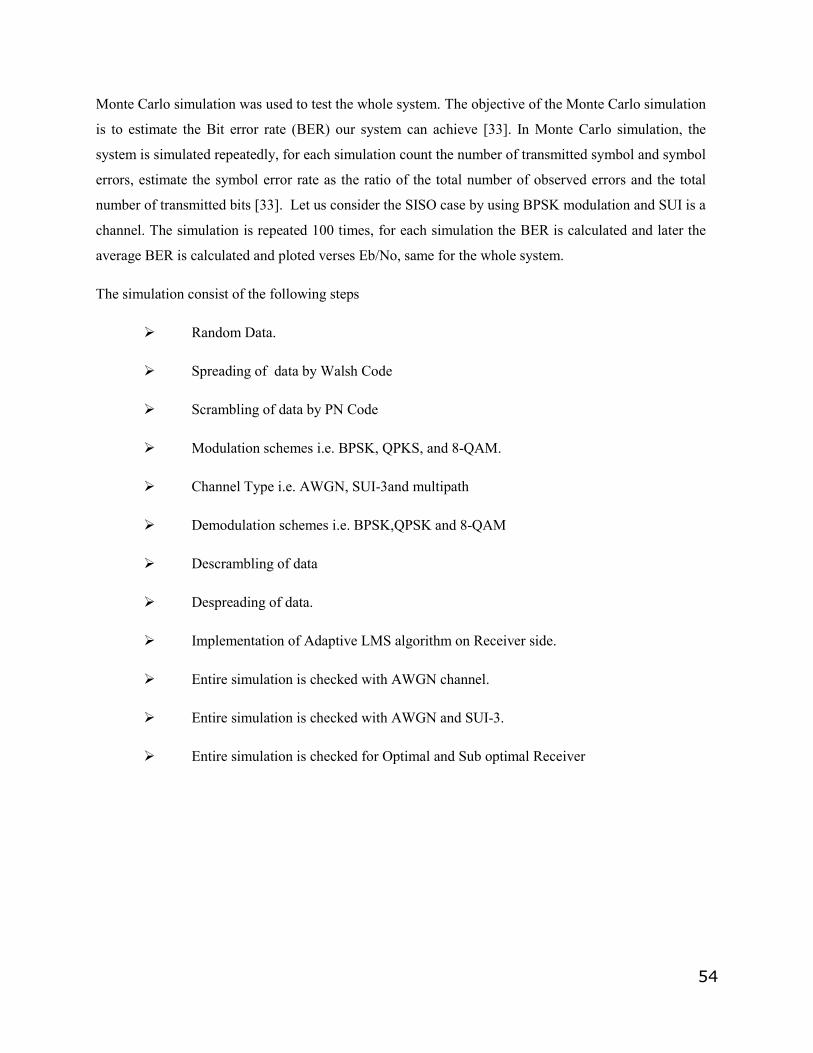
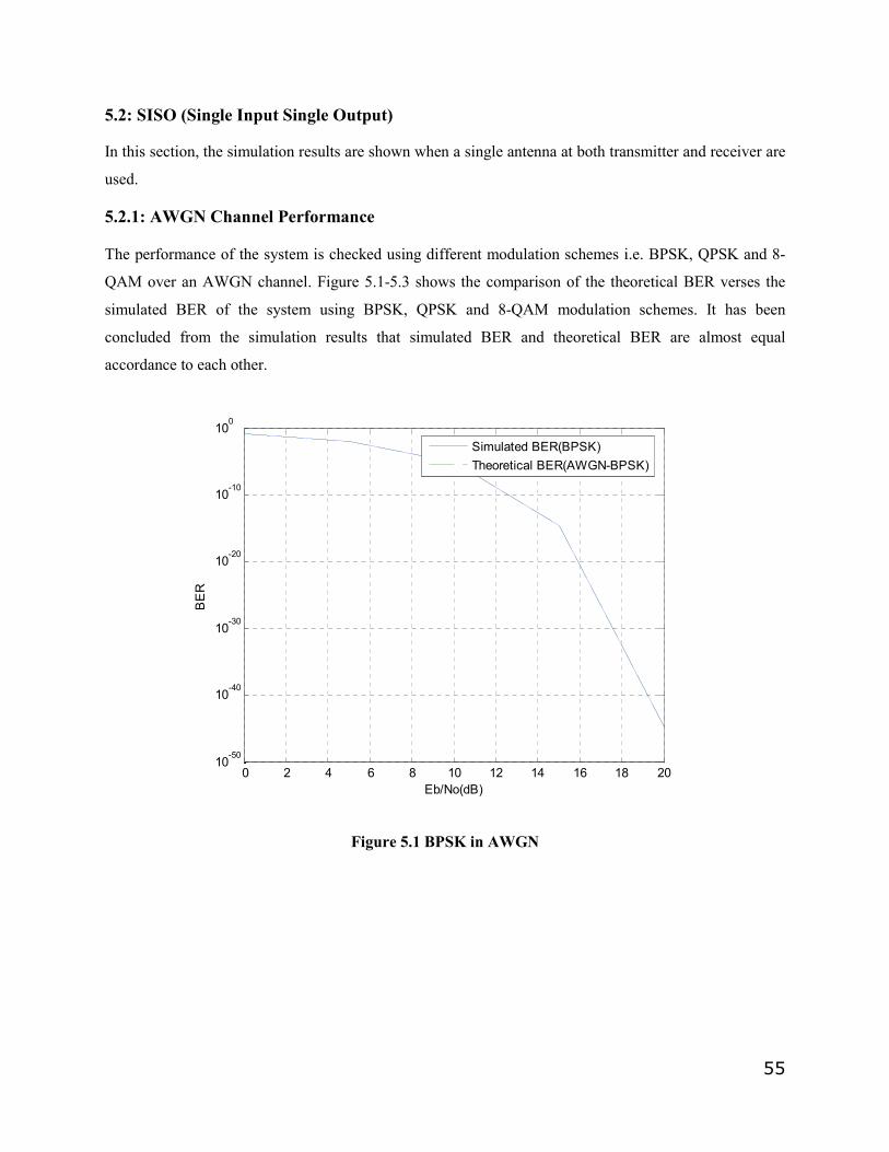
5.2.1: AWGN Channel Performance
The performance of the system is checked using different modulation schemes i.e. BPSK, QPSK and 8-
QAM over an AWGN channel. Figure 5.1-5.3 shows the comparison of the theoretical BER verses the
simulated BER of the system using BPSK, QPSK and 8-QAM modulation schemes. It has been
concluded from the simulation results that simulated BER and theoretical BER are almost equal
accordance to each other.
0 2 4 6 8 10 12 14 16 18 2010
-50
10-40
10-30
10-20
10-10
100
Eb/No(dB)
BER
Simulated BER(BPSK)Theoretical BER(AWGN-BPSK)
Figure 5.1 BPSK in AWGN
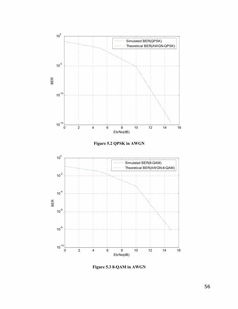
56
0 2 4 6 8 10 12 14 1610
-15
10-10
10-5
100
Eb/No(dB)
BER
Simulated BER(QPSK)Theoretical BER(AWGN-QPSK)
Figure 5.2 QPSK in AWGN
0 2 4 6 8 10 12 14 1610
-10
10-8
10-6
10-4
10-2
100
Eb/No(dB)
BER
Simulated BER(8-QAM)Theoretical BER(AWGN-8-QAM)
Figure 5.3 8-QAM in AWGN
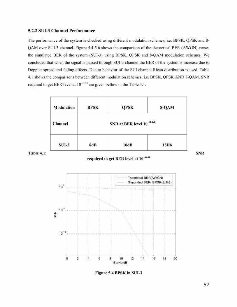
57
5.2.2 SUI-3 Channel Performance
The performance of the system is checked using different modulation schemes, i.e. BPSK, QPSK and 8-
QAM over SUI-3 channel. Figure 5.4-5.6 shows the comparison of the theoretical BER (AWGN) verses
the simulated BER of the system (SUI-3) using BPSK, QPSK and 8-QAM modulation schemes. We
concluded that when the signal is passed through SUI-3 channel the BER of the system is increase due to
Doppler spread and fading effects. Due to behavior of the SUI channel Rican distribution is used. Table
4.1 shows the comparisons between different modulation schemes, i.e. BPSK, QPSK AND 8-QAM. SNR
required to get BER level at 10 -0.44 are given bellow in the Table 4.1.
Table 4.1: SNR required to get BER level at 10 -0.44
0 2 4 6 8 10 12 14 16 18 20
10-10
10-5
100
Eb/No(dB)
BER
Theoritical BER(AWGN)Simulated BER( BPSK-SUI-3)
Figure 5.4 BPSK in SUI-3
Modulation
BPSK
QPSK
8-QAM
Channel
SNR at BER level 10 -0.44
SUI-3
8dB
10dB
15Db
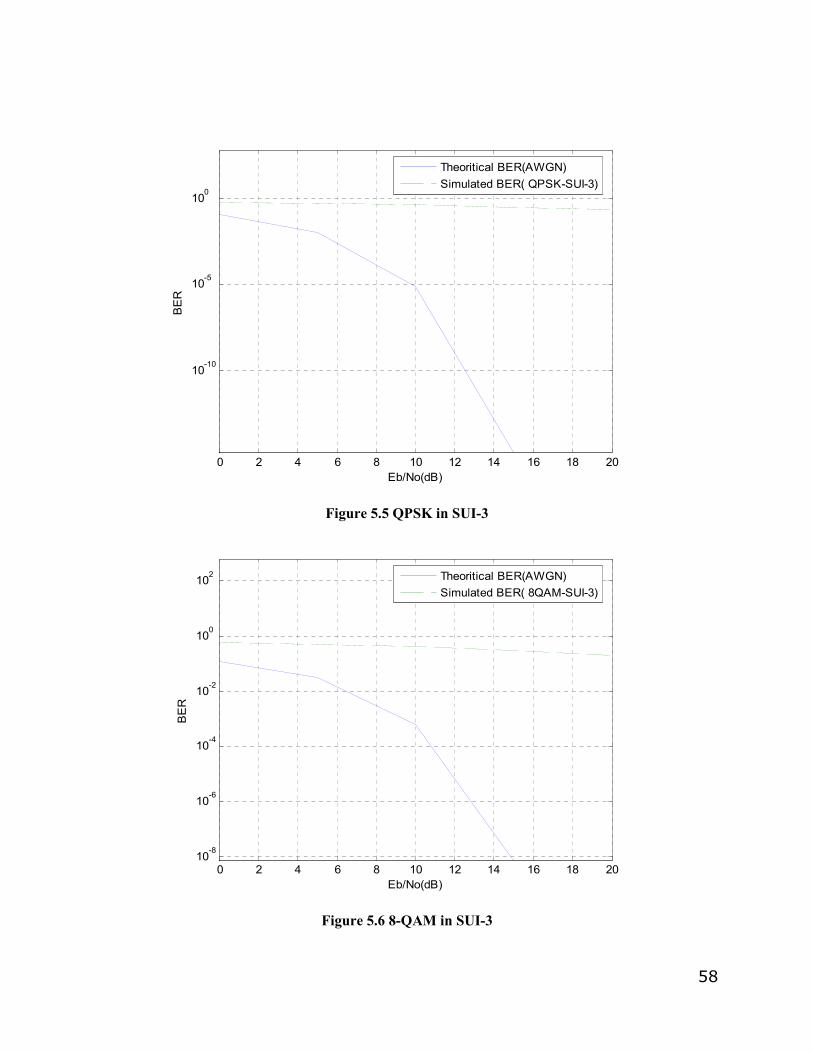
58
0 2 4 6 8 10 12 14 16 18 20
10-10
10-5
100
Eb/No(dB)
BER
Theoritical BER(AWGN)Simulated BER( QPSK-SUI-3)
Figure 5.5 QPSK in SUI-3
0 2 4 6 8 10 12 14 16 18 2010
-8
10-6
10-4
10-2
100
102
Eb/No(dB)
BER
Theoritical BER(AWGN)Simulated BER( 8QAM-SUI-3)
Figure 5.6 8-QAM in SUI-3
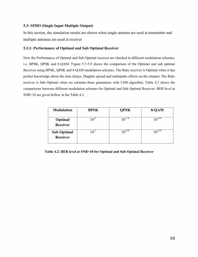
59
5.3: SIMO (Single Input Multiple Output)
In this section, the simulation results are shown when single antenna are used at transmitter and
multiple antennas are used at receiver
5.3.1: Performance of Optimal and Sub Optimal Receiver
Now the Performance of Optimal and Sub Optimal receiver are checked in different modulation schemes,
i.e. BPSK, QPSK and 8-QAM. Figure 5.7-5.9 shows the comparison of the Optimal and sub optimal
Receiver using BPSK, QPSK and 8-QAM modulation schemes. The Rake receiver is Optimal when it has
perfect knowledge about the time delays, Doppler spread and multipaths effects on the channel. The Rake
receiver is Sub Optimal when we estimate these parameters with LMS algorithm. Table 4.2 shows the
comparisons between different modulation schemes for Optimal and Sub Optimal Receiver. BER level at
SNR=10 are given bellow in the Table 4.2.
Table 4.2: BER level at SNR=10 for Optimal and Sub Optimal Receiver
Modulation BPSK QPSK 8-QAM
Optimal Receiver
10-2 10-1.8 10-0.8
Sub Optimal Receiver
10-1 10-0.8 10-0.4
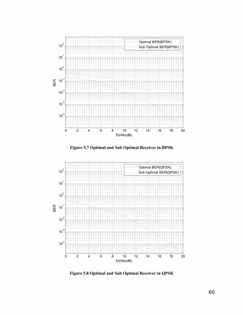
60
0 2 4 6 8 10 12 14 16 18 20
10-4
10-3
10-2
10-1
100
101
102
Eb/No(dB)
BER
Optimal BER(BPSK)Sub Optimal BER(BPSK)
Figure 5.7 Optimal and Sub Optimal Receiver in BPSK
0 2 4 6 8 10 12 14 16 18 20
10-4
10-3
10-2
10-1
100
101
102
Eb/No(dB)
BER
Optimal BER(QPSK)Sub Optimal BER(QPSK)
Figure 5.8 Optimal and Sub Optimal Receiver in QPSK
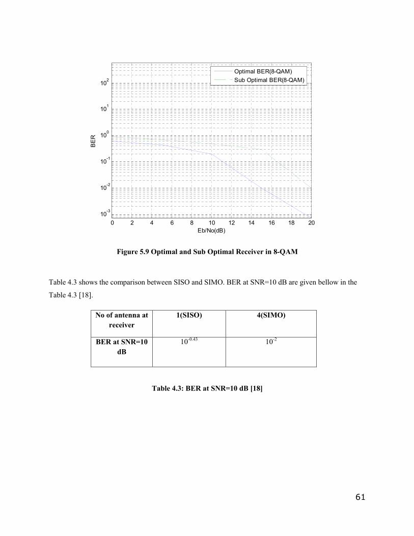
61
0 2 4 6 8 10 12 14 16 18 2010
-3
10-2
10-1
100
101
102
Eb/No(dB)
BER
Optimal BER(8-QAM)Sub Optimal BER(8-QAM)
Figure 5.9 Optimal and Sub Optimal Receiver in 8-QAM
Table 4.3 shows the comparison between SISO and SIMO. BER at SNR=10 dB are given bellow in the
Table 4.3 [18].
No of antenna at receiver
1(SISO) 4(SIMO)
BER at SNR=10 dB
10-0.43 10-2
Table 4.3: BER at SNR=10 dB [18]
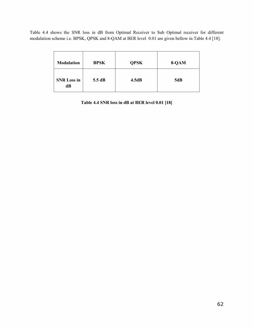
62
Table 4.4 shows the SNR loss in dB from Optimal Receiver to Sub Optimal receiver for different modulation scheme i.e. BPSK, QPSK and 8-QAM at BER level 0.01 are given bellow in Table 4.4 [18].
Table 4.4 SNR loss in dB at BER level 0.01 [18]
Modulation
BPSK
QPSK
8-QAM
SNR Loss in dB
5.5 dB
4.5dB
5dB
63
Chapter 6: Conclusions and Future work
6.1: Conclusion
These chapter summaries the conclusion of thesis works. It also presents the possible future work.
Study of different Rake receivers and implemented three fingers Rake receiver in matlab.
Study of the Walsh code and implemented in Matlab.
Study of the spreading with Walsh code and implemented in Matlab.
Study of the Pseudo Noise (PN) code and implemented in Matlab.
Study of the scrambling with PN code and implemented in Matlab.
Study of the SUI-3 channel model and implemented in Matlab.
Study different Adaptive channel estimation algorithms. Adaptive LMS algorithm is implemented in
Matlab due of its simple implementation.
BPSK having Less BER than QPSK and 8-QAM, but BPSK require low bandwidth and low signal
power.
QPSK having less BER than 8-QAM but high than BPSK. QPSK require higher bandwidth and signal
power than BPSK.
8-QAM having high BER than BPSK and QPSK but require higher bandwidth and signal power than
BPSK and QPSK.
Fading is a well know major problem in wireless communication systems. In this thesis multipath fading
is considered in SUI-3 channel model. According to the behavior of the SUI-3 channel Rician distribution
is used. To reduce the fading effects in SUI model the Adaptive LMS algorithm is implemented at the
receiver side. Three-finger rake Receiver is implemented to capture three strongest multipaths, one LOS
signal and two NLOS signals.
The Average SNR loss from Optimal receiver to Sub Optimal Receiver for different modulation schemes
i.e. BPSK, QPSK and 8-QAM is 5dB, which is quite good in the simulation.
Finally it has been concluded form simulation result that adaptive LMS algorithm implemented on
Receiver side reduce the BER of the system in great extent.
64
6.2: Future work
THE model used in the thesis is SIMO (simple Input Multiple output). In future the authors would like to
work on MIMO (Multiple Input Multiple output).
The channel estimation algorithm used in the thesis is Adaptive LMS. In future the authors would like to
implements others channel estimation algorithms like Adaptive MMSE, Adaptive MLSE and Adaptive
RLS algorithm.
In future the authors would like to work on Normalized LMS (NLMS) to improve the convergence speed
in a non-static environment.
In future the authors would like to work on Long Term Evaluation (LTE) and High Altitude
Platform (HAP) systems.
65
Reference
[1] Karim M.R., Saraaf Mohsen, “W-CDMA and CDMA 2000 for 3G mobile networks”
[2] http://www.celusion.com/whitepapers/fdma_tdma_cdma.htm
[3] Yang Samuel C, “CDMA RF system engineering”, Artech House London 1998, ISBN 0-89006-991-3
[4] Chandran, N.; Valenti, M.C, “Three generations of cellular wireless systems”, Potentials, IEEE
Volume 20, Issue 1, Feb/Mar 2001.
[5] Riaz Esmailzadeh and Masao Nakagawa, “TDD-CDMA for Wireless Communications”, Artech
House London 2002.
[6] 3GPP TS 25.221 V5.5.0 (2003-6), “Physical Channels and mapping of transport channels onto
physical channels (TDD)”
[7] 3GPP TR 25.928 V4.01 – 1.28, “Functionality for UTRA TDD Physical Layer”, Release 4, 2001
[8] http://cp.literature.agilent.com/litweb/pdf/5989-5734ZHA.pdf
[9] http://www.exp-math.uni-essen.de/~vinck/crypto/7-random-number-generators.doc
[10] Jhong Sam Lee and Leonard E. Miller, “CDMA Systems Engineering Handbooks”, Artech house
mobile communication library 1998, ISBN 0-89006-990-5
[11] Ahsan Aziz, “Channel Estimation for a WCDMA Rake Receiver”, Freescale Semiconductor
Application Note, Rev. 2, 11/2004
[12] http://www.wirelesscommunication.nl/reference/chaptr05/mccdma/mcm1.htm
[13] Geoff Smithson, “Introduction to Digital Modulation Schemes”, [Online]. Available:
http://www.plextek.co.uk/papers/schmsv6.pdf
[14] Wikipedia the free encyclopedia, “Amplitude-Shift Keying (ASK)”, Available: Wikipedia online:
http://en.wikipedia.org/wiki/Amplitude-shift_keying
[15] Search Networking, “Phase Shift Keying”, Available: SearchNetworking.com online:
http://searchnetworking.techtarget.com/sDefinition/0,,sid7_gci213937,00.html
[16] Hp Hewlett Packard, “Digital Modulation in Communications Systems –An Introduction”, Application Note 1298, 5965-7160E
66
[17] Tech FAQ, “What is Quadrature Amplitude Modulation”, [Online]. Available: http://www.tech-
faq.com/quadrature-amplitude-modulation.shtml
[18] V. Erceg, K.V.S. Hari, M.S. Smith, D.S. Baum et al, “Channel Models for Fixed Wireless
Applications”, IEEE 802.16.3 Task Group Contributions 2001, Feb. 01
[19] Book, S. Rappaport, “Wireless Communications Principles and Practice”, Second Edition.
[20] http://www.wirelesscommunication.nl/reference/chaptr03/fading/delayspr.htm
[21] Wikipedia the free encyclopedia, “Path loss”, Available: Wikipedia online:
http://en.wikipedia.org/wiki/Pathloss
[22] http://zone.ni.com/devzone/cda/ph/p/id/334
[23] Online Education, “Smart Antenna Systems,” 2003 International Engineering Consortium.
http://www.iec.org/online/tutorials/smart_ant/topic01.html
[24] http://www.wirelesscommunication.nl/reference/chaptr05/digimod/awgn.htm
[25] Ammar Osman, “Low- complexity OFDM Transceiver design for UMTS- LTE”, Blekinge institute
of technology, January 2007, MEE07:10
[26] http://www.conniq.com/Glossary_D.htm
[27] B.Farhang-Boroujeny,”Adaptive Filters theory and applications”, John wiley and sons 1999, ISBN
0-471-98337-3.
[28] http://etd.lib.fsu.edu/theses/available/etd-04092004-143712/unrestricted/Ch_6lms.pdf
[29] Y. Li, “Simplified channel estimation for OFDM systems with multiple transmit antennas”, IEEE
Transactions on Wireless Communications, vol.1, No.1, pp.67-75, Jan. 2002
[30] A. Petropulu, R. Zhang and R. Lin, “Blind OFDM Channel Estimation Through Simple Linear
Precoding”, IEEE Transactions on Wireless Communications, vol.3, No.2, pp.647-655, Mar. 2004
[31]http://users.ece.utexas.edu/~bevans/courses/ee381k/projects/spring05/wang/FinalProjectReport.pdf
[32] www.it.lut.fi/mat/kesakoulu/yorgon.../adaptive_filtering_chapter4.ppt
67
[33] Dr. B.-P. Paris, Simulation of Wireless Communication Systems using MATLAB, fall 2007.