1

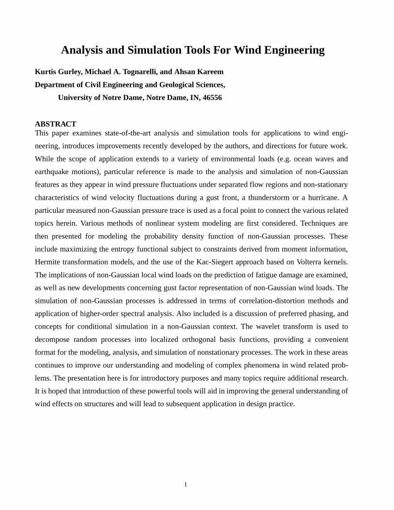
ABSTRACTThis paper examines state-of-the-art analysis and simulation tools for applications to wind engi-

neering, introduces improvements recently developed by the authors, and directions for future work.

While the scope of application extends to a variety of environmental loads (e.g. ocean waves and

earthquake motions), particular reference is made to the analysis and simulation of non-Gaussian

features as they appear in wind pressure fluctuations under separated flow regions and non-stationary

characteristics of wind velocity fluctuations during a gust front, a thunderstorm or a hurricane. A

particular measured non-Gaussian pressure trace is used as a focal point to connect the various related

topics herein. Various methods of nonlinear system modeling are first considered. Techniques are

then presented for modeling the probability density function of non-Gaussian processes. These

include maximizing the entropy functional subject to constraints derived from moment information,

Hermite transformation models, and the use of the Kac-Siegert approach based on Volterra kernels.

The implications of non-Gaussian local wind loads on the prediction of fatigue damage are examined,

as well as new developments concerning gust factor representation of non-Gaussian wind loads. The

simulation of non-Gaussian processes is addressed in terms of correlation-distortion methods and

application of higher-order spectral analysis. Also included is a discussion of preferred phasing, and

concepts for conditional simulation in a non-Gaussian context. The wavelet transform is used to

decompose random processes into localized orthogonal basis functions, providing a convenient

format for the modeling, analysis, and simulation of nonstationary processes. The work in these areas

continues to improve our understanding and modeling of complex phenomena in wind related prob-

lems. The presentation here is for introductory purposes and many topics require additional research.

It is hoped that introduction of these powerful tools will aid in improving the general understanding of

wind effects on structures and will lead to subsequent application in design practice.

Analysis and Simulation Tools For Wind Engineering

Kurtis Gurley, Michael A. Tognarelli, and Ahsan Kareem

Department of Civil Engineering and Geological Sciences,

University of Notre Dame, Notre Dame, IN, 46556

g load

ssues.

tacitly

ed prima-

sses is

essure

ong non-

he non-

xpected

wind

e regions

skewed

ussian

t due to

turbu-

of the

ts in the

faces.

s may

areem et

ed the

a on the

parated

l scales

Letch-

wind

spectral

ctuating

ysis of

hen the

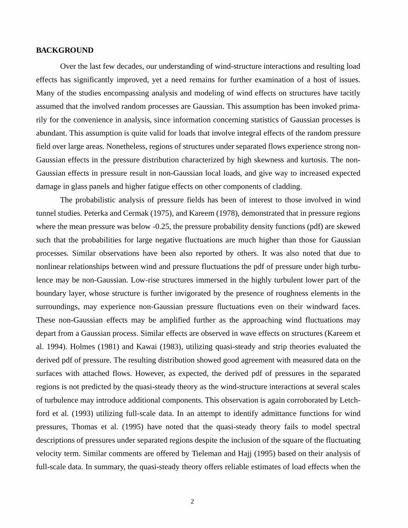
BACKGROUND

Over the last few decades, our understanding of wind-structure interactions and resultin

effects has significantly improved, yet a need remains for further examination of a host of i

Many of the studies encompassing analysis and modeling of wind effects on structures have

assumed that the involved random processes are Gaussian. This assumption has been invok

rily for the convenience in analysis, since information concerning statistics of Gaussian proce

abundant. This assumption is quite valid for loads that involve integral effects of the random pr

field over large areas. Nonetheless, regions of structures under separated flows experience str

Gaussian effects in the pressure distribution characterized by high skewness and kurtosis. T

Gaussian effects in pressure result in non-Gaussian local loads, and give way to increased e

damage in glass panels and higher fatigue effects on other components of cladding.

The probabilistic analysis of pressure fields has been of interest to those involved in

tunnel studies. Peterka and Cermak (1975), and Kareem (1978), demonstrated that in pressur

where the mean pressure was below -0.25, the pressure probability density functions (pdf) are

such that the probabilities for large negative fluctuations are much higher than those for Ga

processes. Similar observations have been also reported by others. It was also noted tha

nonlinear relationships between wind and pressure fluctuations the pdf of pressure under high

lence may be non-Gaussian. Low-rise structures immersed in the highly turbulent lower part

boundary layer, whose structure is further invigorated by the presence of roughness elemen

surroundings, may experience non-Gaussian pressure fluctuations even on their windward

These non-Gaussian effects may be amplified further as the approaching wind fluctuation

depart from a Gaussian process. Similar effects are observed in wave effects on structures (K

al. 1994). Holmes (1981) and Kawai (1983), utilizing quasi-steady and strip theories evaluat

derived pdf of pressure. The resulting distribution showed good agreement with measured dat

surfaces with attached flows. However, as expected, the derived pdf of pressures in the se

regions is not predicted by the quasi-steady theory as the wind-structure interactions at severa

of turbulence may introduce additional components. This observation is again corroborated by

ford et al. (1993) utilizing full-scale data. In an attempt to identify admittance functions for

pressures, Thomas et al. (1995) have noted that the quasi-steady theory fails to model

descriptions of pressures under separated regions despite the inclusion of the square of the flu

velocity term. Similar comments are offered by Tieleman and Hajj (1995) based on their anal

full-scale data. In summary, the quasi-steady theory offers reliable estimates of load effects w

2

e scale

effects

eory is

babi-

eling of

ers and

pressure

ed wind

of basis

titutive

ulation

tput is

loading

n many

r func-

ressure

tening

resent a

s of a

s (e.g.,

). These

ns. For

y

dominant mode of loading is attributed to buffeting, e.g., surface pressures responding to larg

or low frequency turbulence. However, the pressures resulting from wind-structure interaction

cannot be predicted from the quasi-steady theory. A departure from the quasi-steady th

reflected in the non-Gaussian pressure field.

In light of the established inability of quasi-steady theory to predict the dynamics and pro

listic structure of pressure fluctuations in the separated regions, some thoughts on the mod

non-Gaussian processes are presented. This approach holds promise for providing answ

perhaps models for situations in which the quasi-steady theory has failed to do so because

fluctuations are a result of a nonlinear dynamic interaction.

The analysis of nonstationary processes such as transient wind gusts in short, measur

records has been limited due to shortcomings in the Fourier analysis. Here, we apply a set

functions local in both time and frequency to decompose the signal into octave-banded cons

parts. The wavelet transform is useful in the location of energy transfer in time, and in the sim

of nonstationary processes.

MODELING OF NON-GAUSSIAN PROCESSES

In the study of physical systems, the relationship between the input and the system ou

often sought to model the system response. For linear systems, e.g., in the formulation of gust

factors, such a relationship is used for the prediction of extreme response (Davenport, 1964). I

instances in wind engineering, however, the input and output are not related by a linear transfe

tion due to nonlinear characteristics, e.g., the turbulent fluctuations in a hurricane, negative p

fluctuations on building envelopes and associated fatigue of cladding and, in particular, its fas

system. Many approaches are available for modeling nonlinearly related processes. Here we p

brief look at Volterra series systems, as well as several other alternatives.

Volterra Systems

In the Volterra series formulation, the input-output relationship may be expressed in term

hierarchy of linear, quadratic and higher-order transfer functions or impulse response function

Schetzen, 1980, Kareem and Li, 1988, Spanos and Donley, 1991, Kareem and Zhao, 1994

transfer functions can be determined from experimental data or from theoretical consideratio

example, a nonlinear system modeled by Volterra’s stochastic series expansion is described b

, (1)y t( ) h1 τ( )x t τ–( )dτ h2 τ1 τ2,( )x t τ1–( )x t τ2–( )dτ1dτ2 …+∫∫+∫=

3

where and are the first and second-order impulse response functions.

The Fourier transform of the Volterra series expansion up to second order (retaining two terms

on the right hand side) in Eq. 1 gives the response in the frequency domain as

. (2)

For linear systems, the first term on the right hand side of Eq. 2 is all that is needed to describe

the relationship between input and output. This linear model assumes that the Fourier components at

different frequencies are uncoupled. In the first (linear) term on the right hand side of Eq. 2, the

response at frequency is dependent only on input and the transfer function at frequency .

In the case where the system is nonlinear, the Fourier components are coupled, and additional

terms are needed to capture this interaction. The second term on the right hand side of Eq. 2 couples

the response at frequency with pairs of input components at frequencies whose sum or differ-

ence is through the quadratic transfer function (QTF) . Equation 2 describes a system

whose nonlinear component is non-symmetric with respect to the probability density function (e.g. an

even powered polynomial nonlinearity). A third-order system captures the behavior of systems with

both symmetric and non-symmetric nonlinearities (e.g. polynomial nonlinearities with odd and even

powers).

In the case when input and output of a system is available, the information can be

used to estimate the Volterra kernels in Eq. 2 directly. The linear transfer function is given by

. (3)

where is the expected value operator. Here, the numerator is the cross-power spectrum of the

input and output in terms of their Fourier transforms and , and the denomina-

tor is the auto-power spectrum of the input.

Just as is derived from the cross-power spectrum, the QTF is derived from a higher-

order cross-spectrum. The higher-order cross-spectrum between the input and the output

needed to estimate the QTF is called the cross-bispectrum, denoted . Analogous to the

cross-power spectrum in the numerator of Eq. 3, the cross-bispectrum can be expressed in terms of

the expected value of input and output Fourier components as

. (4)

The QTF is given by

h1 τ( ) h2 τ1 τ2,( )

Y fi( ) H1 fi( )X fi( ) H2 f1 f2,( )X f1( )X f2( )f1 f2+ fi=

∑+=

Y fi( ) fi fi

Y fi( ) fifi H2 f1 f2,( )

x n( ) y n( )

H1 fi( )X∗ fi( )Y fi( )⟨ ⟩

X fi( ) 2⟨ ⟩--------------------------------=

⟨ ⟩

x n( ) y n( ) Y f( ) X f( )

H1 fi( )

x n( ) y n( )

Bxxy f1 f2,( )

Bxxy f1 f2,( ) X∗ f1( )X∗ f2( )Y f1 f2+( )⟨ ⟩=

4

. (5)

If no phase coupling exists between and and , then their phases will be ran-

dom and independent, thus the net expected value of the cross-bispectrum will be zero. The formula-

tion for the QTF given in Eq. 5 is valid for a Gaussian input process . The linear and quadratic

transfer functions can also be estimated for a general random input, i.e., without assuming particular

statistics of the input (e.g., Nam, et al., 1990).

Equation 2 addresses a second-order Volterra system, which assumes the nonlinearity is asym-

metric. More generally, higher-order spectral analysis may be applied to nonlinear system identifica-

tion via the higher-order transfer function, which may then be used with a Volterra series similar to

Eq. 2 with additional higher-order terms to model the nonlinear system.

The analogies between the power spectrum and higher-order spectra may be extended to glean

some insight into their physical meaning. The significance of the power spectrum is well

understood to be the decomposition of the signal variance as a function of frequency. Simi-

larly, the bispectrum may be viewed as the decomposition of skewness as a

function of two frequencies, and the trispectrum as the decomposition of kurtosis

as a function of three frequencies. The volumes under the bispectrum and trispectrum yield

the third and fourth central moments, respectively. When viewed in this light, it is apparent that the

existence of higher-order spectra indicates a deviation from Gaussian.

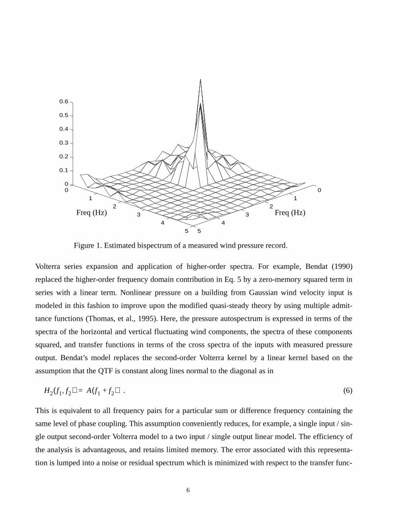
An estimated bispectrum for an experimentally measured wind pressure record is shown in

Fig. 1. This nonzero bispectrum indicates a deviation from Gaussian due to interaction between low

frequency components. For a quadratic nonlinear process that is a square of a narrow-banded linear

process, the bispectrum contains peaks where components of the linear process interact at their sum

and difference frequencies, imparting energy at those frequencies to the resulting nonlinear process.

In this case, the bispectrum does not consist only of sharp peaks, indicating that the pressure record is

not the result of the square of a narrow-banded process, but more likely the output of an at least

partially quadratic system with a wide-banded input. The input process in this case is in fact a wide-

banded wind velocity process. Were it the case that pressure was the result of a cubic nonlinearity

acting on the wind velocity, the bispectrum would not exist, and the trispectrum would reveal the

symmetrically nonlinear relation of the pressure to velocity.

Alt ernatives to Volterra Systems

Several researchers have addressed the modeling of nonlinear systems by means other than a

H2 f1 f2,( ) 12---=

Bxxy f1 f2,( )

X f1( )X f2( ) 2⟨ ⟩-------------------------------------

Y f1 f2+( ) X f1( ) X f2( )

X f( )

Sxx f1( )

x2

t( )⟨ ⟩

Bxxx f1 f2,( ) x3

t( )⟨ ⟩

Txxxx f1 f2 f3, ,( )

x4

t( )⟨ ⟩

5

(1990)

term in

put is

dmit-

s of the

onents

ressure

on the

g the

ut / sin-

cy of

resenta-

r func-

Volterra series expansion and application of higher-order spectra. For example, Bendat

replaced the higher-order frequency domain contribution in Eq. 5 by a zero-memory squared

series with a linear term. Nonlinear pressure on a building from Gaussian wind velocity in

modeled in this fashion to improve upon the modified quasi-steady theory by using multiple a

tance functions (Thomas, et al., 1995). Here, the pressure autospectrum is expressed in term

spectra of the horizontal and vertical fluctuating wind components, the spectra of these comp

squared, and transfer functions in terms of the cross spectra of the inputs with measured p

output. Bendat’s model replaces the second-order Volterra kernel by a linear kernel based

assumption that the QTF is constant along lines normal to the diagonal as in

. (6)

This is equivalent to all frequency pairs for a particular sum or difference frequency containin

same level of phase coupling. This assumption conveniently reduces, for example, a single inp

gle output second-order Volterra model to a two input / single output linear model. The efficien

the analysis is advantageous, and retains limited memory. The error associated with this rep

tion is lumped into a noise or residual spectrum which is minimized with respect to the transfe

0

1

2

3

4

5

0

1

2

3

4

5

0

0.1

0.2

0.3

0.4

0.5

0.6

Figure 1. Estimated bispectrum of a measured wind pressure record.

Freq (Hz)Freq (Hz)

H2 f1 f2,( ) A f1 f2+( )=

6

t

tions describing the linear systems in parallel. The nonlinearity is represented, but the assumption of

its form may be restrictive for some systems. The model may be modified to facilitate the input of

non-Gaussian wind velocity (Bendat, 1990).

Neural Networks

Another recently developed approach to nonlinear system modeling is the application of

neural networks. A multi-layered set of processing elements receives input information and uses the

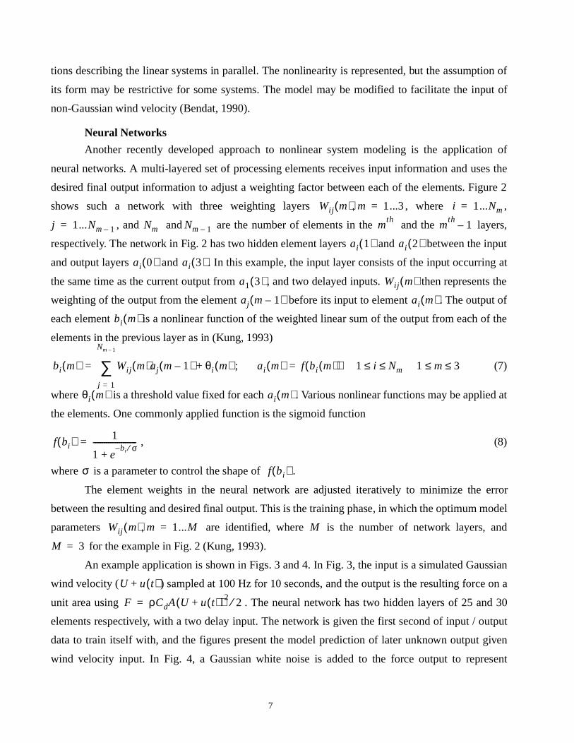
desired final output information to adjust a weighting factor between each of the elements. Figure 2

shows such a network with three weighting layers , where ,

, and and are the number of elements in the and the layers,

respectively. The network in Fig. 2 has two hidden element layers and between the input

and output layers and . In this example, the input layer consists of the input occurring at

the same time as the current output from , and two delayed inputs. then represents the

weighting of the output from the element before its input to element . The output of

each element is a nonlinear function of the weighted linear sum of the output from each of the

elements in the previous layer as in (Kung, 1993)

; (7)

where is a threshold value fixed for each . Various nonlinear functions may be applied a

the elements. One commonly applied function is the sigmoid function

, (8)

where is a parameter to control the shape of .

The element weights in the neural network are adjusted iteratively to minimize the error

between the resulting and desired final output. This is the training phase, in which the optimum model

parameters are identified, where is the number of network layers, and

for the example in Fig. 2 (Kung, 1993).

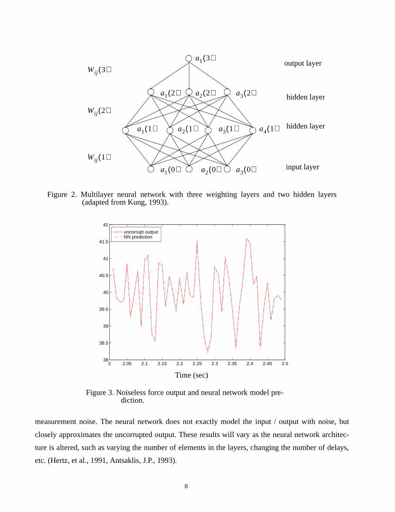
An example application is shown in Figs. 3 and 4. In Fig. 3, the input is a simulated Gaussian

wind velocity ( ) sampled at 100 Hz for 10 seconds, and the output is the resulting force on a

unit area using . The neural network has two hidden layers of 25 and 30

elements respectively, with a two delay input. The network is given the first second of input / output

data to train itself with, and the figures present the model prediction of later unknown output given

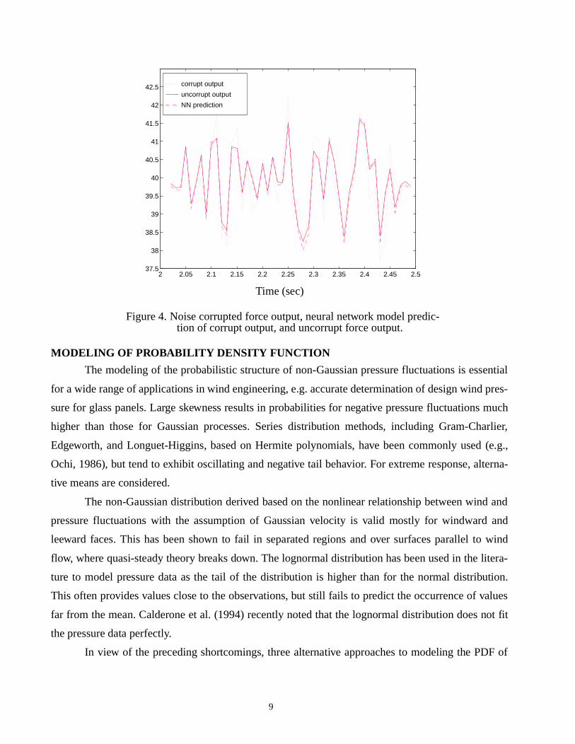
wind velocity input. In Fig. 4, a Gaussian white noise is added to the force output to represent

Wij m( ) m, 1...3= i 1...Nm=

j 1...Nm 1–= Nm Nm 1– mth

mth

1–

ai 1( ) ai 2( )

ai 0( ) ai 3( )

a1 3( ) Wij m( )

aj m 1–( ) ai m( )

bi m( )

bi m( ) Wij m( )aj m 1–( ) θi m( )+

j 1=

Nm 1–

∑= ai m( ) f bi m( )( )= 1 i Nm≤ ≤ 1 m 3≤ ≤

θi m( ) ai m( )

f bi( ) 1

1 ebi σ⁄–

+-----------------------=

σ f bi( )

Wij m( ) m, 1...M= M

M 3=

U u t( )+

F ρCdA U u t( )+( )2 2⁄=

7

se, but

rchitec-

delays,

measurement noise. The neural network does not exactly model the input / output with noi

closely approximates the uncorrupted output. These results will vary as the neural network a

ture is altered, such as varying the number of elements in the layers, changing the number of

etc. (Hertz, et al., 1991, Antsaklis, J.P., 1993).

Figure 2. Multilayer neural network with three weighting layers and two hidden layers(adapted from Kung, 1993).

Wij 1( )

Wij 2( )

Wij 3( )

a1 1( ) a2 1( ) a3 1( ) a4 1( )

a1 0( )

a1 2( )

a1 3( )

a2 2( )

a2 0( )

a3 2( )

a3 0( )

output layer

input layer

hidden layer

hidden layer

uncorrupt outputNN prediction

2 2.05 2.1 2.15 2.2 2.25 2.3 2.35 2.4 2.45 2.538

38.5

39

39.5

40

40.5

41

41.5

42

Figure 3. Noiseless force output and neural network model pre-diction.

Time (sec)

8

sential

d pres-

s much

harlier,

d (e.g.,

lterna-

nd and

and

to wind

litera-

ution.

values

not fit

DF of

MODELING OF PROBABILITY DENSITY FUNCTION

The modeling of the probabilistic structure of non-Gaussian pressure fluctuations is es

for a wide range of applications in wind engineering, e.g. accurate determination of design win

sure for glass panels. Large skewness results in probabilities for negative pressure fluctuation

higher than those for Gaussian processes. Series distribution methods, including Gram-C

Edgeworth, and Longuet-Higgins, based on Hermite polynomials, have been commonly use

Ochi, 1986), but tend to exhibit oscillating and negative tail behavior. For extreme response, a

tive means are considered.

The non-Gaussian distribution derived based on the nonlinear relationship between wi

pressure fluctuations with the assumption of Gaussian velocity is valid mostly for windward

leeward faces. This has been shown to fail in separated regions and over surfaces parallel

flow, where quasi-steady theory breaks down. The lognormal distribution has been used in the

ture to model pressure data as the tail of the distribution is higher than for the normal distrib

This often provides values close to the observations, but still fails to predict the occurrence of

far from the mean. Calderone et al. (1994) recently noted that the lognormal distribution does

the pressure data perfectly.

In view of the preceding shortcomings, three alternative approaches to modeling the P

corrupt output

uncorrupt output

NN prediction

2 2.05 2.1 2.15 2.2 2.25 2.3 2.35 2.4 2.45 2.537.5

38

38.5

39

39.5

40

40.5

41

41.5

42

42.5

Figure 4. Noise corrupted force output, neural network model predic-tion of corrupt output, and uncorrupt force output.

Time (sec)

9

e

non-Gaussian pressure fluctuations in separated regions are considered here. The Maximum Entropy

Method (MEM), Hermite transformation based models and Kac Siegert expansion based models ar

applied to the pressure records through their statistical moments or quadratic transfer function to

determine the parameters of the respective estimation models. Applications of these methods are

il lustrated by way of two examples.

Maximum Entropy Method

An approach to approximate the pdf of nonlinear systems is the Maximum Entropy Method

(MEM), in which the Shannon entropy functional is maximized subject to constraints in the form of

moment information. In the limiting case of infinite moment information, a unique PDF is defined. In

reality, we will always have a finite amount of moment information for which an infinite number of

probability density functions are admissible. The pdf which maximizes the entropy functional is the

least biased estimate for the given moment information. The Lagrange multiplier method is applied to

solve this variational problem, and provides the joint pdf of higher-order systems directly. A brief

outline of MEM is presented here. Complete details can be found in Sobczyk and Trebicki (1990);

Kareem and Zhao (1994); Kapur (1988).

The available information for a process can be expressed as the process joint moments

, (9)

where is the order of the system. , where is the maximum order or correla-

tion moment, is the joint pdf, and is the value of the joint moment. The integral is multi-

fold to . One possible pdf of the process is that which maximizes the entropy functional,

, (10)

subject to constraints from the moment information.

After application of the Lagrange multiplier method, the resulting description of for an

-dimensional case is

. (11)

Substitution of Eq. 11 into the moment constraints and an additional normalization constraint

gives the following system of equations.

, and (12)

y t( )

E y1r1y2

r2...ynrn[ ] ... y1

r1y2r2...yn

rnp y( )dy∫∫ mr1...rn= =

n ri 0 1 2 ... M, , , ,= M

p y( ) mr1...rn

n y t( )

H p y( ) lnp y( )dy∫–=

p y( )

n

p y( ) exp λ– 0 1–( )exp λr1...rny1

r1...ynrn

r1 ... rn+ +

M

∑–

=

p y( )dy∫ 1=

y1r1...yn

rnexp λr1...rny1

r1...ynrn

r1 ... rn+ +

M

∑–

dy∫ mr1...rn=

10

M

. (13)

This system of nonlinear integral equations is solved numerically and the results yield the

least biased estimate of the system joint pdf under the given moment constraints using Eq. 11

(Sobczyk and Trebicki, 1990; Kareem and Zhao, 1994). The moment information which constrains

the maximum entropy functional may be in the form of moment equations rather than moment values

as presented above. Details are omitted here; interested readers may refer to Sobczyk and Trebicki

(1990).

Moment Based Hermite Transformation Model

This approach is based on a functional transformation of a standardized non-Gaussian

process, , to a standard Gaussian process, , (e.g., Grigoriu, 1984)

. (14)

Several choices of are possible to preserve only the first four moments. A cubic model of

offers a convenient and fairly accurate representation (Winterstein, 1988). Accordingly, the pdf

of is given by (Grigoriu, 1984; Winterstein, 1988)

, (15)

, (16)

where , , , ,

, , , and and are the

skewness and kurtosis of the fluctuating process, which reduce to zero for Gaussian. An improvement

to this model is suggested here by using the expressions for and given previously (which are

approximations) as initial conditions for solving the following pair of nonlinear algebraic equations:

, (17)

. (18)

These equations have been derived for use in this study by setting the third-and fourth-order central

exp λr1...rny1

r1...ynrn

r1 ... rn+ +

∑–

dy∫ exp λ0 1+( )=

x t( ) u t( )

x t( ) X t( ) X–( ) σX⁄ g u t( )[ ]= =

g u( )

g u( )

x t( )

pX x( ) 1

2π----------exp

u2

x( )2

-------------–du x( )

dx--------------=

u x( ) ξ2x( ) c+ ξ x( )+[ ]

1 3⁄ξ2

x( ) c+ ξ x( )–[ ]1 3⁄

a––=

ξ x( ) 1.5b axα---+

a3–= a

h3

3h4

--------= b1

3h4

--------= c b 1– a2–( )

3=

h3γ3

4 2 1 1.5γ4++---------------------------------------= h4

1 1.5γ4+ 1–

18-----------------------------------= α 1

1 2h32

6h42

+ +-------------------------------------= γ3 γ4

h3 h4

γ3 α3 8h33 108h3h4

2 36h3h4 6h3+ + +( )=

γ4 3+ α4 60h34 3348h4

4 2232h32h4

2 60h32 252h4

2+ + + +(=

1296h43 576h3

2h4 24h4 3)+ + + +

11

moments of equal to the known central moments of . This yields new coefficient values

which exactly match the statistics up to the fourth order of the modeled non-Gaussian process. This is

referred to herein as the modified Hermite method.

The transformation above is for the case when is a softening process, for example, the

response of a linear system subjected to nonlinear viscous drag force. Winterstein (1988) also outlines

a transformation for the case in which is a hardening process. This development is not repeated

here, but such a situation could arise, for example, if the structural system is characterized by a

nonlinear stiffness.

Kac-Sieger t Approach

Once a system has been modeled in terms of a Volterra series (Eq. 1), different approaches are

available to estimate the pdf of the process. One such approach is that of Kac and Siegert (1947). In

this approach, the system output is expressed in terms of the sum of standardized normal random vari-

ates and their squares as described below (e.g. Naess, 1985; Langley, 1987; Kareem and Zhao,

1994)

. (19)

The parameter is related to the eigenvectors , and are the eigenvalues of the Fredholm inte-

gral equation of the second kind given by

, (20)

where is the QTF discussed earlier, and the frequency domain counterpart of ,

and is a two-sided spectrum of the underlying linear process.

The characteristic equation of is now expressed as

, where (21)

The pdf of the process is the Fourier transform of the characteristic function

. (22)

In general, Eq. 22 cannot be solved in closed form, and must be numerically estimated. This represen-

tation of a non-Gaussian pdf is most appropriate for non-Gaussian systems resulting from a quadratic

transformation. Any other transformation must be recast in a quadratic form to obtain best results.

The cumulant of a random process is defined in terms of the characteristic function

g u t( )[ ] x t( )

x t( )

x t( )

Xj

y t( ) BjXj λjXj2+( )

j 1=

2N

∑=

Bj ψj λ j

K ω1 ω2,( )∫ ψj ω2( )dω2 λ jψj ω1( )= K ω1 ω2,( ) H ω1 ω2,( ) S ω1( )S ω2( )=

H ω1 ω2,( ) h2 τ τ2,( )

S ω( )

x

M θ( ) Mj θ( )j 1=

2N

∏= Mj θ( ) 1 2iλ j–( ) 1 2⁄–exp

Bj2θ2

2 1 2iλjθ–( )------------------------------–=

x

p x( ) 12π------ e

iθx–M θ( )dθ

∞–

∞

∫=

nth

kn y

12

and after appropriate substitutions is given by

, (23)

where is zero for , and unity otherwise. These cumulants may be used as coefficients in a

series expansion of the pdf, or as constraints in the Maximum Entropy Method.

Examples

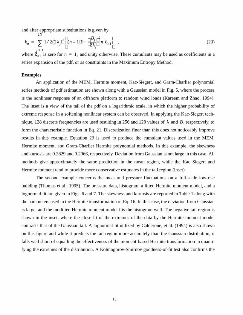
An application of the MEM, Hermite moment, Kac-Siegert, and Gram-Charlier polynomial

series methods of pdf estimation are shown along with a Gaussian model in Fig. 5, where the process

is the nonlinear response of an offshore platform to random wind loads (Kareem and Zhao, 1994).

The inset is a view of the tail of the pdf on a logarithmic scale, in which the higher probability of

extreme response in a softening nonlinear system can be observed. In applying the Kac-Siegert tech-

nique, 128 discrete frequencies are used resulting in 256 and 128 values of and , respectively, to

form the characteristic function in Eq. 21. Discretization finer than this does not noticeably improve

results in this example. Equation 23 is used to produce the cumulant values used in the MEM,

Hermite moment, and Gram-Charlier Hermite polynomial methods. In this example, the skewness

and kurtosis are 0.3829 and 0.2066, respectively. Deviation from Gaussian is not large in this case. All

methods give approximately the same prediction in the mean region, while the Kac Siegert and

Hermite moment tend to provide more conservative estimates in the tail region (inset).

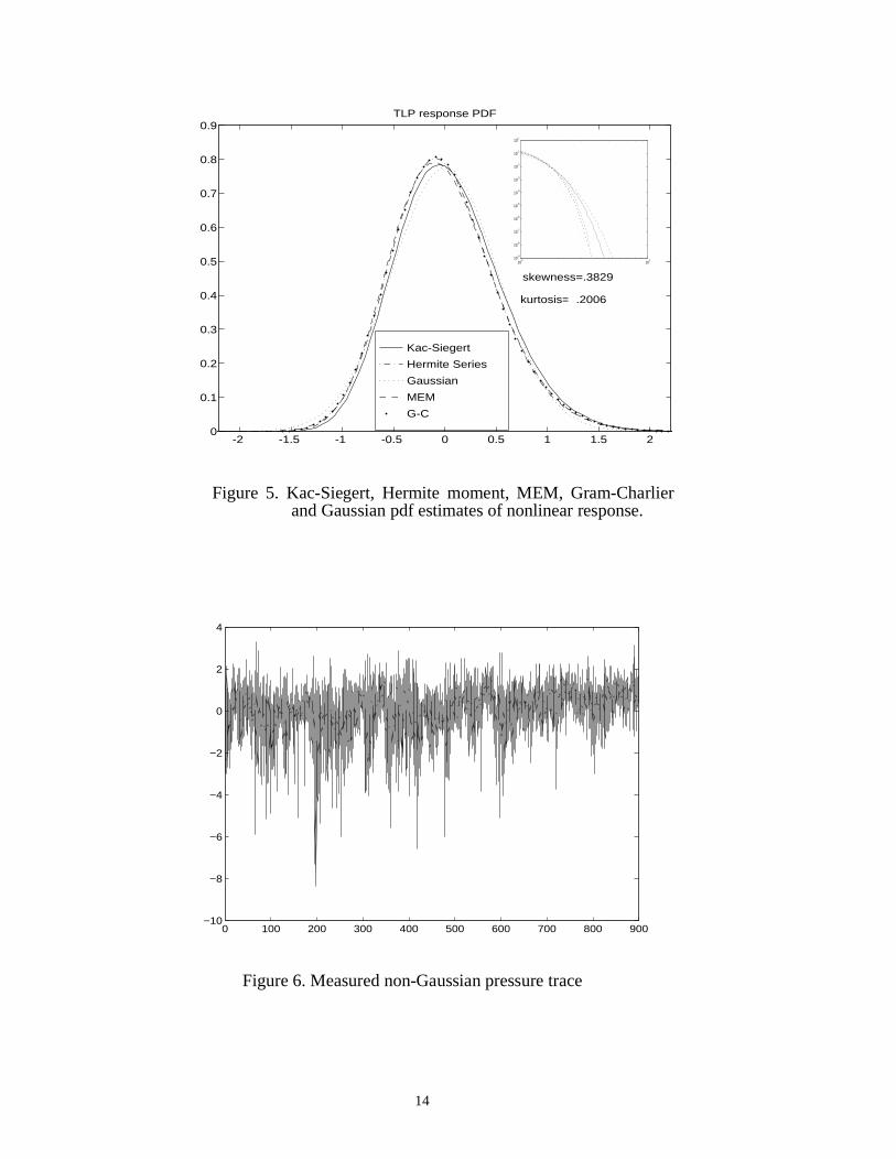
The second example concerns the measured pressure fluctuations on a full-scale low-rise

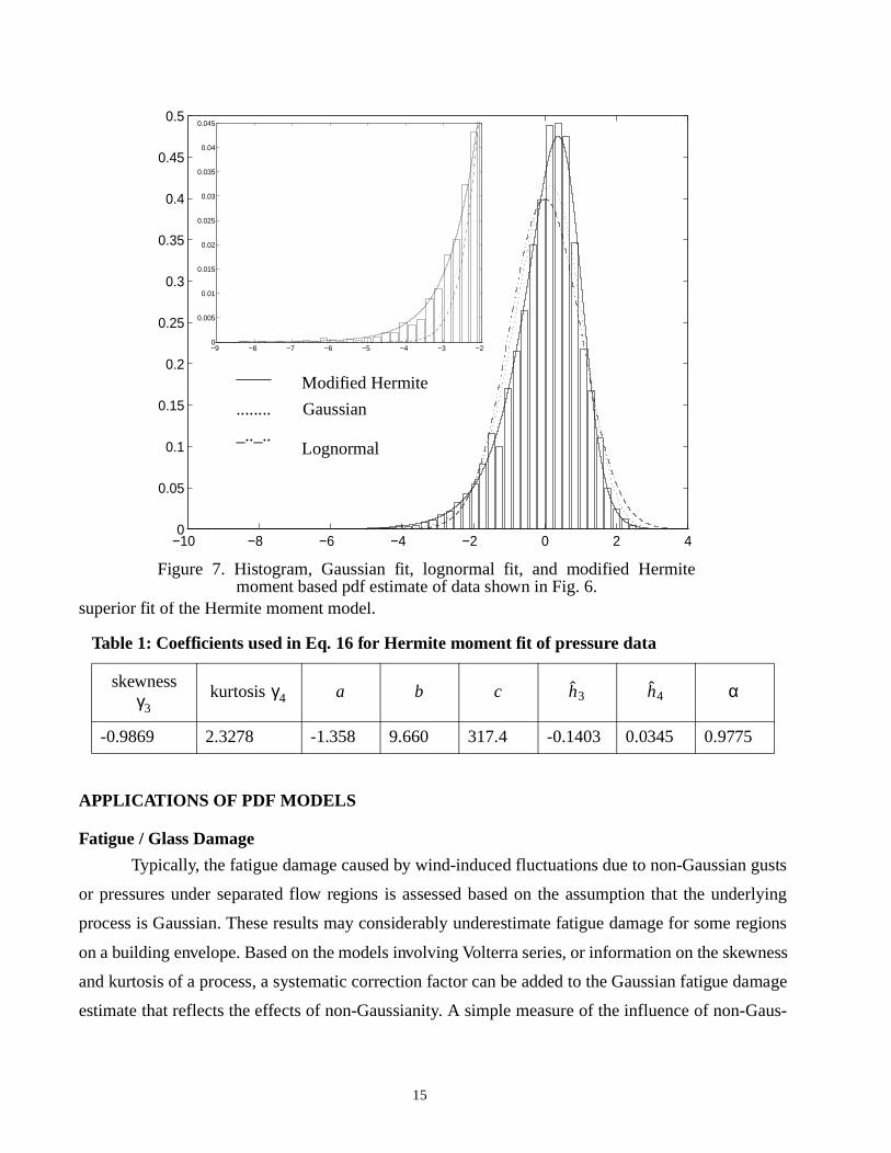
building (Thomas et al., 1995). The pressure data, histogram, a fitted Hermite moment model, and a

lognormal fit are given in Figs. 6 and 7. The skewness and kurtosis are reported in Table 1 along with

the parameters used in the Hermite transformation of Eq. 16. In this case, the deviation from Gaussian

is large, and the modified Hermite moment model fits the histogram well. The negative tail region is

shown in the inset, where the close fit of the extremes of the data by the Hermite moment model

contrasts that of the Gaussian tail. A lognormal fit utilized by Calderone, et al. (1994) is also shown

on this figure and while it predicts the tail region more accurately than the Gaussian distribution, it

falls well short of equalling the effectiveness of the moment-based Hermite transformation in quanti-

fying the extremes of the distribution. A Kolmogorov-Smirnov goodness-of-fit test also confirms the

kn 1 2⁄ 2λj( )nn 1–( )!

Bj

2λj--------

2n!δn1+

j 1=

2N

∑=

δn1 n 1=

λ B

13

Kac-Siegert

Hermite Series

Gaussian

MEM

G-C

-2 -1.5 -1 -0.5 0 0.5 1 1.5 20

0.1

0.2

0.3

0.4

0.5

0.6

0.7

0.8

0.9TLP response PDF

skewness=.3829

kurtosis=3.2006

100

101

10-9

10-8

10-7

10-6

10-5

10-4

10-3

10-2

10-1

100

Figure 5. Kac-Siegert, Hermite moment, MEM, Gram-Charlierand Gaussian pdf estimates of nonlinear response.

0 100 200 300 400 500 600 700 800 900−10

−8

−6

−4

−2

0

2

4

Figure 6. Measured non-Gaussian pressure trace

14

gusts

nderlying

e regions

wness

damage

-Gaus-

superior fit of the Hermite moment model.

APPLICATIONS OF PDF MODELS

Fatigue / Glass Damage

Typically, the fatigue damage caused by wind-induced fluctuations due to non-Gaussian

or pressures under separated flow regions is assessed based on the assumption that the u

process is Gaussian. These results may considerably underestimate fatigue damage for som

on a building envelope. Based on the models involving Volterra series, or information on the ske

and kurtosis of a process, a systematic correction factor can be added to the Gaussian fatigue

estimate that reflects the effects of non-Gaussianity. A simple measure of the influence of non

Table 1: Coefficients used in Eq. 16 for Hermite moment fit of pressure data

skewness kurtosis

-0.9869 2.3278 -1.358 9.660 317.4 -0.1403 0.0345 0.9775

Figure 7. Histogram, Gaussian fit, lognormal fit, and modified Hermitemoment based pdf estimate of data shown in Fig. 6.

−10 −8 −6 −4 −2 0 2 40

0.05

0.1

0.15

0.2

0.25

0.3

0.35

0.4

0.45

0.5

−9 −8 −7 −6 −5 −4 −3 −20

0.005

0.01

0.015

0.02

0.025

0.03

0.035

0.04

0.045

____

........

_.._..

Modified Hermite

Gaussian

Lognormal

γ3γ4 a b c h3 h4 α

15

sian effects on fatigue damage accumulation is the ratio of fatigue damage under non-Gaussian

loading to that under Gaussian loading

. (24)

This ratio, based on Hermite moment transformation models for non-Gaussian narrow-banded pro-

cesses, is given by Winterstein (1988) as

; . (25)

Where , , and and have been defined in Eq 16. Utiliz-

ing the non-Gaussian pressure fluctuation data in Fig. 6, is equal to 1.6. This could potentially

enhance fatigue of cladding components by sixty percent. The assumption of normality may lead to

unconservative fatigue life prediction when the actual response is non-Gaussian with a kurtosis value

greater than zero. However, conservative estimates are expected for non-Gaussian cases with a kurto-

sis value less than zero.

The importance of non-Gaussian local pressures on cladding glass has been addressed by,

among others, Holmes (1985), Reed (1993), and Calderone and Melbourne (1993). Holmes (1985)

and Reed (1993) utilized a non-Gaussian distribution of pressure fluctuations based on the relation-

ship between Gaussian wind velocity and non-Gaussian pressure variations. This relationship is based

on quasi-steady theory which has its limits but works well for stagnation face pressure. Numerical

simulations involving wind tunnel data have revealed that non-Gaussian fluctuations result in greater

glass damage. The cumulative damage criterion is used to determine the effect of fluctuating pressure

through an equivalent constant pressure. Beside the nonlinear relationship between the pressure and

resulting stress in glass, the glass size, and its geometry, the non-Gaussian features of pressure fluctu-

ations play an important role in determining the cumulative damage. The equivalent constant pressure

is given by (Holmes, 1985).

, (26)

where is the duration of the equivalent pressure (60 seconds in the U.S.), is the pressure at a

particular instant, is the total number of instants being accumulated, is the time duration of pres-

sure , is the slope of the straight line on a log-log scale of the plot between pressure and surface

tensile strength of glass, and is dependent on the type of glass (Calderone and Melbourne, 1993). In

the second expression for , is the length of the sample considered and is the pdf of the

λE Dng[ ]E Dg[ ]------------------=

λ πk2Vs!-----------

m mVs( )!

m 2⁄( )!------------------

= Vs4π--- 1 h4 h4+ +( ) 1–=

h4 γ4 24⁄= k 1 2h32

6h42

+ +( )1– 2⁄

= h3 h4

λ

pE1

TE------ pi

snti

i 1=

l

∑

1sn-----

Ts1

TE------ psnfP p( ) pd

∞–

∞

∫

1sn-----

= =

TE pi

l t i

pi s

n

pE TS fP p( )

16

e data,

oment

8. For

nge for

ficance

of the

orld-

mption

aussian

nport’s

stiffer

t factor,

,

ly to

reem &

e more

geworth

le as a

of the

itive

s and

f the

pressure process. Using a histogram of a sample of data to represent the pdf of th

the ratio of for the non-Gaussian model to Gaussian is equal to 1.84. Using the Hermite m

model, this ratio is 1.76 and using a lognormal model (Calderone, et al., 1994) the ratio is 1.1

comparison’s sake, the limits of the integration have been taken to be the end points of the ra

which pressure data is available in the realization of data considered. This illustrates the signi

of non-Gaussian effects in the evaluation of and more importantly the effectiveness

moment-based Hermite transformation in capturing this significance.

Gust Factors

The use of gust factors to account for the dynamics of wind fluctuations is accepted w

wide. The concept, based on the original formulation by Davenport (1964), relies on the assu

of a Gaussian process. For dynamic pressures resulting from the square of wind velocity the G

assumption may break down. Soize (1978) and Kareem & Zhao (1994) have extended Dave

Gaussian model to include non-Gaussian effects, which are more pronounced for relatively

structures. The non-Gaussian contribution also increases for high levels of turbulence. The gus

, relates the mean of the extremes of a process to the mean of the parent process as follows

, (27)

where is the peak factor. When , we simply have and we need mere

compute the peak factor. The peak factor used in the non-Gaussian gust factor formulation (Ka

Zhao, 1994) employs the moment-based Hermite transformation which has been shown to b

accurate in representing the tail regions of the pdf of a non-Gaussian process than the Ed

series employed by Soize (1978). Treating the standardized non-Gaussian random variab

nonlinear function of a Gaussian random variable as in Eq. 14, the probability density function

process may be readily derived (e.g., Ang & Tang, 1975).

According to Cartwright and Longuet-Higgins (1956), the distribution of all maxima (pos

and negative) of the standardized Gaussian process are given as,

, (28)

where, is a descriptor of the bandwidth of the parent Gaussian proces

the can be described in terms of moments of the one-sided spectral density o

TS 900s=( )

pE

pE

G

Xex X gσ+ X 1gσ

X---------+

GX= = =

g X 0= Xex gσ=

X

pUmaxu( ) 1

2π---------- εexp

u2

2ε2--------–

1 ε2– uexpu2

2-----–

expξ2

2-----–

dξ

∞–

u1 ε2–

ε------------------

∫+=

ε 1 m22

m0m4( )⁄–=

mi

17

(33)

process, , where n is frequency in Hertz. For a narrow-banded process, , and

Eq. 28 yields the Rayleigh distribution.

The cumulative distribution of the extremes of the parent Gaussian process is (e.g. Davenport,

1964; Ang & Tang, 1984),

, (29)

where is the expected number of maxima during an interval of length, T (e.g.,

Madsen, et. al, 1986), and from Eq. 28, assuming that u is large, we may approximate (Cartwright &

Longuet-Higgins, 1956),

, (30)

which leaves,

. (31)

So, we have for the extremes of ,

. (32)

The peak factor, , relates the mean of the positive extreme values of to its standard

deviation. To compute it, we must first determine . Making the assumption in Eq. 30, we

have for the case when is zero mean ,

, and . This gives,

. (34)

In order to evaluate Eq. 34, we must develop the form of . This is accomplished by first

solving for , according to,

. (35)

Since the time, , is usually very large, an asymptotic expansion for Eq. 35 is,

, (36)

where . Substituting Eq. 36 into the moment-based Hermite transformation model and

mi niS n( )dn0

∞∫= ε 0=

PUexu( ) exp N 1 PUmax

u( )–( )–[ ]=

N m4 m2⁄ T=

1 PUmaxu( ) 1 ε2– exp

u2

2-----–

O1u3-----exp

u2

2ε2--------–

+

m2

m0m4

------------------expu2

2-----–

≈≈–

PUexu( ) exp m2 m0⁄ Texp

u2

2-----–

–=

X

PXexx( ) exp m2 m0⁄ Texp

u2 x( )2

-------------– –=

gNG X

dPXexx( )

X

dPXexx( ) exp ψ–( )dψ= ψ ν0Texp u2 x( ) 2⁄–[ ]= ν0 m2 m0⁄=

Xex x ψ( )exp ψ–( )dψ0

∞

∫ gNGσX= =

x ψ( )

u x( )

u x( ) 2lnν0T 2lnψ–=

T

u x( ) β lnψβ

---------lnψ( )2

2β3----------------– …+–=

β 2lnν0T=

18

retaining terms of and greater, yields,

, (37)

where, (Euler’s constant), and is the zero-upcrossing rate, , ,

are functions of skewness and kurtosis. For Gaussian processes, and and

which reduces Eq. 37 to the standard Gaussian form given by Davenport (1967). For the 900 s realiza-

tion of data in Fig. 6, . The peak factor based on Eq. 37 using statistical information de-

rived from the data is equal to -7.4, whereas the corresponding value for the Gaussian case is -3.9. It is

important to note that Eq. 37 is for positive extremes and for the negative extremes which we have

considered here, the opposite of the skewness value must be used.

By comparison, Cheong (1995) treats exceedence of a threshold which lies two standard devi-

ations below the mean as a separate random variable. By choosing a low threshold, successive

exceedences may be considered independent. The occurrence of exceedences of the threshold is

modeled as a Poisson process and the distribution of exceedences is modeled by an exponential distri-

bution. From this model, the distribution of the largest exceedence, , for a duration, , is derived as,

, (38)

where and may be obtained from data as the reciprocals of the mean exceedence and the mean

inter-exceedence interval, respectively. In terms of the distribution parameters, the expected value and

the most probable value of the maximum exceedence are given by

, . (39)

Thus, the expected minimum and its most probable minimum are

, . (40)

For the data considered above, , . These values approach the

peak factor attained by using the moment-based Hermite transformation model, but are somewhat less

conservative in their estimate of the extreme value. This can be noted in Figs. 6 and 7.

In a recent study, Krayer and Marshall (1992) have pointed out that the linear gust factor based

on extratropical storms may underestimate the gust factor for hurricane conditions. It is quite clear

that the hurricane wind field comprised of turbulence due to convective processes superimposed upon

O β 1–( )

gNG k β γβ---+

h3 β2 2γ 1–+( ) h4 β3 3β γ 1–( ) 3β---+ +

π2

12------ γ–

γ2

2----+

+ +

=

γ 0.5772= β 2l n νoT( )= νo k h3

h4 h3 h4 0= α 1=

ν0 1.334=

S t

PS t( ) s( ) e θte µs––=

µ θ

E S t( )[ ] ln θt( ) 0.5772+µ-------------------------------------= Smp

ln θt( )µ---------------=

Cp

E Cp t( )[ ] Cp 2σCp– E S t( )[ ]–= Cpmp

Cp 2σCp– Smp–=

E Cp t( )[ ] 7.019–= Cpmp6.562–=

19

ange in

fferent

troduce

ination

a.

diction

reasing

ries of

tics. The

, 1971;

ress in

rocesses

995).

ssian

desired

transfor-

t spec-

elation

hematic

. This

nner &

inearity

terms

a large, coherent vertical structure results in non-Gaussian fluctuations. Near the ground, a ch

energy distribution with respect to frequency may result from nonlinear interactions between di

frequency components. Changes in the pdf and the power spectral density would certainly in

changes in the statistics of velocity fluctuations, leading to a larger gust factor. A closer exam

using a theory based on the preceding comments is being pursued to model the observed dat

SIMULATION OF NON-GAUSSIAN PROCESSES

Among a host of approximate analytical techniques developed for the analysis and pre

of nonlinear system response, simulation methods are becoming more attractive due to the inc

ability of high speed computers. For implementation of time domain schemes, the time histo

loading functions are generated in accordance with desired statistical and spectral characteris

simulation procedures for Gaussian random processes are well established (Shinozuka

Mignolet and Spanos, 1987; Li and Kareem, 1993; Soong and Grigoriu, 1993). However, prog

the simulation of non-Gaussian processes has been elusive. A recent book on non-Gaussian p

provides an excellent overview of current methods of non-Gaussian simulation (Grigoriu, 1

Several promising methods currently being pursued by the authors are presented here.

Correlation-Distortion Method

An approach used by Yamazaki & Shinozuka (1988) for the simulation of non-Gau

processes begins with the simulation of a Gaussian process which is then transformed to the

non-Gaussian process through the following mapping

. (41)

An iterative procedure is necessary to match the desired target spectrum since the nonlinear

mation in Eq. 41 also modifies the spectral contents.

The necessity for an iterative procedure may be eliminated if one begins with the targe

trum or auto-correlation of the non-Gaussian process and transforms it to the underlying corr

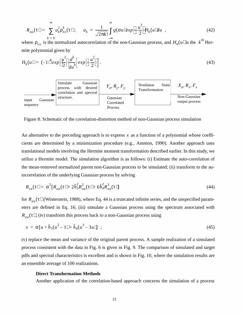
of the Gaussian process (Gurley and Kareem, 1995). Then, a simulation based on the sc

shown in Fig. 8 would eliminate the spectral distortion caused by the nonlinear transformation

approach is referred to as the correlation-distortion method in stochastic system literature (Co

Hammond, 1979; Deutsch, 1962; and Johnson, 1994). For a given static single-valued nonl

,where is a standard normal Gaussian process, the desired autocorrelation of in

of can be expressed as (Deutsch, 1962)

X t( ) Fx1– Φ y( ){ }=

x g u( )= u x

y

20

e

∞ ∞

; , (42)

where is the normalized autocorrelation of the non-Gaussian process, and is the Her-

mite polynomial given by

. (43)

An alternative to the preceding approach is to express as a function of a polynomial whose coeffi-

cients are determined by a minimization procedure (e.g., Ammon, 1990). Another approach uses

translational models involving the Hermite moment transformation described earlier. In this study, we

utilize a Hermite model. The simulation algorithm is as follows: (i) Estimate the auto-correlation of

the mean-removed normalized parent non-Gaussian process to be simulated; (ii) transform to the au-

tocorrelation of the underlying Gaussian process by solving

(44)

for (Winterstein, 1988), where Eq. 44 is a truncated infinite series, and the unspecified param-

eters are defined in Eq. 16; (iii) simulate a Gaussian process using the spectrum associated with

; (iv) transform this process back to a non-Gaussian process using

; (45)

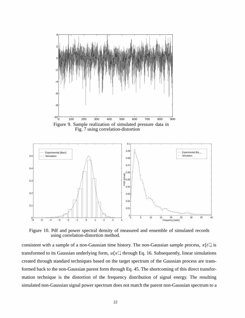
(v) replace the mean and variance of the original parent process. A sample realization of a simulated

process consistent with the data in Fig. 6 is given in Fig. 9. The comparison of simulated and target

pdfs and spectral characteristics is excellent and is shown in Fig. 10, where the simulation results ar

an ensemble average of 100 realizations.

Direct Transformation Methods

Another application of the correlation-based approach concerns the simulation of a process

Ruu τ( ) ak2ρxx

k τ( )k 0=

∑= ak1

2πk!---------------- g σu( )exp

u2

2-----–

Hk u( )du

∞–

∫=

ρxx Hk u( ) kth

Hk u( ) 1–( )kexp

u2

2-----

dk

duk

-------- expu

2

2-----–

=

input Gaussiansequence

Simulate Gaussianprocess with desiredcorrelation and spectralstructure.

Nonlinear StaticTransformation

GaussianCorrelatedProcess

Yn Ry Fy, , Xn Rx Fx, ,

Non-Gaussianoutput process

Figure 8. Schematic of the correlation-distortion method of non-Gaussian process simulation

x

Rxx τ( ) α2Ruu τ( ) 2h3

2Ruu

2 τ( ) 6h42Ruu

3 τ( )+ +[ ]=

Ruu τ( )

Ruu τ( )

x α u h3 u2 1–( ) h4 u

3 3u–( )+ +[ ]=

21

, is

lations

are trans-

ansfor-

ulting

trum to a

ords

consistent with a sample of a non-Gaussian time history. The non-Gaussian sample process,

transformed to its Gaussian underlying form, , through Eq. 16. Subsequently, linear simu

created through standard techniques based on the target spectrum of the Gaussian process

formed back to the non-Gaussian parent form through Eq. 45. The shortcoming of this direct tr

mation technique is the distortion of the frequency distribution of signal energy. The res

simulated non-Gaussian signal power spectrum does not match the parent non-Gaussian spec

0 100 200 300 400 500 600 700 800 900-10

-8

-6

-4

-2

0

2

4

Figure 9. Sample realization of simulated pressure data inFig. 7 using correlation-distortion

Experimental (Bars)Simulation

−6 −5 −4 −3 −2 −1 0 1 2 3 40

0.1

0.2

0.3

0.4

0.5

Experimental (Bars)Simulation

0 5 10 15 20 25 30 35 400

0.01

0.02

0.03

0.04

0.05

0.06

0.07

0.08

0.09

0.1

Frequency [rad/s]

PS

D [s/

rad

]

Figure 10. Pdf and power spectral density of measured and ensemble of simulated recusing correlation-distortion method.

x t( )

u x( )

22

t

r

satisfactory degree. This distortion may stem from the inability of the three-term truncated Hermite

moment transformation in Eq. 16 to produce a Gaussian signal for cases when the parent signal is

highly non-Gaussian. The linear simulation is then based on a target spectrum derived from a process

which is assumed Gaussian, but is not. It is at this point where the frequency information is distorted,

and results in poor simulations. One option for improved results is to add terms to the Hermite series

until a Gaussian transformation is achieved. This may require a different number of terms to achieve

accuracy for varying input sample signals.

A simple correction has been suggested to remove this distortion in the direct transformation

method (Gurley and Kareem, 1995). Referring to Eq. 16, it can be seen that the governing parameters

and thus are dependent on the skewness and kurtosis. and may be

treated as adjustable input parameters in order to force the transformed process, , to be Gaussian.

Optimization of these two parameters is based on the minimization of the function

, (46)

where and are the skewness and kurtosis of the inverse Hermite transformed process .

The optimized input parameters and now provide a Gaussian process, and the linear simula-

tions do not contain distortion. The same parameters are used to transform back to a non-Gaussian

simulation whose pdf and power spectral density closely match those of the parent process. This cor-

rection is essentially a quantification of the error in truncating the Hermite series after the third order.

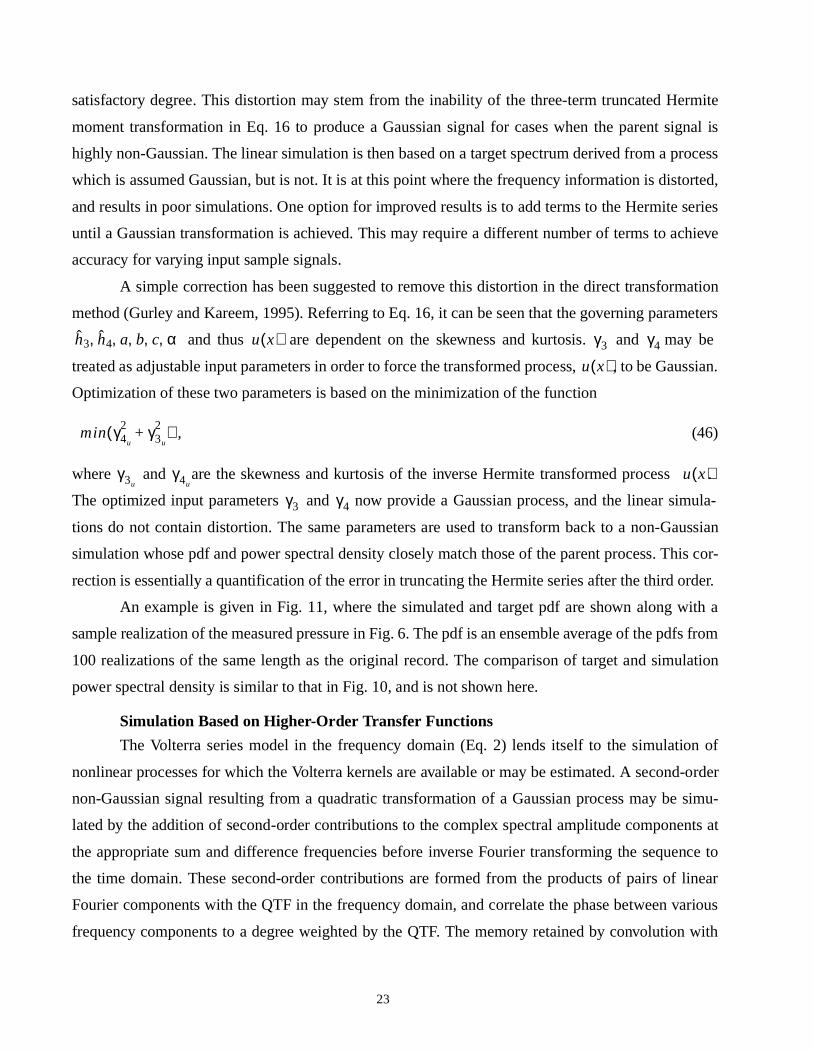
An example is given in Fig. 11, where the simulated and target pdf are shown along with a

sample realization of the measured pressure in Fig. 6. The pdf is an ensemble average of the pdfs from

100 realizations of the same length as the original record. The comparison of target and simulation

power spectral density is similar to that in Fig. 10, and is not shown here.

Simulation Based on Higher-Order Transfer Functions

The Volterra series model in the frequency domain (Eq. 2) lends itself to the simulation of

nonlinear processes for which the Volterra kernels are available or may be estimated. A second-order

non-Gaussian signal resulting from a quadratic transformation of a Gaussian process may be simu-

lated by the addition of second-order contributions to the complex spectral amplitude components a

the appropriate sum and difference frequencies before inverse Fourier transforming the sequence to

the time domain. These second-order contributions are formed from the products of pairs of linea

Fourier components with the QTF in the frequency domain, and correlate the phase between various

frequency components to a degree weighted by the QTF. The memory retained by convolution with

h3 h4 a b c α, , , , , u x( ) γ3 γ4

u x( )

min γ4u

2 γ3u

2+( )

γ3uγ4u

u x( )

γ3 γ4

23

um and

ase of

tionally.

terac-

informa-

derlying

presence

ussian

cesses

odel.

with a

r Volterra

The use

ion. A

red wind

ulated

revious

arity in

essure

the QTF facilitates the simulation of processes that are able to match not only the power spectr

pdf of the parent process, but the bispectrum as well.

This approach requires information concerning the QTF of the desired process. In the c

non-Gaussian waves and their loads on offshore structures, the QTFs can be derived computa

However, in the case of wind effects this is not possible due to the complexity of nonlinear in

tions that take place as turbulent wind encounters a structure. In the absence of the necessary

tion, it is possible to estimate a QTF based on the desired process and an extracted un

Gaussian process. Such an attempt is made here using the pressure data in Fig. 6. Due to the

of higher-order nonlinearities, an estimated QTF may not completely model the non-Ga

features. This concept in principle may easily be extended to the simulation of nonlinear pro

beyond the second order, where higher-order information, e.g. trispectrum, may improve the m

A simulation based on a QTF extracted from pressure data is shown in Fig. 12, along

sample of the measured data, and indeed reflects a lack of completeness in the second orde

model. The model fails to properly reflect the skewness and kurtosis of the measured record.

of higher order transfer functions is currently being researched to improve upon the simulat

second example is shown in Fig. 13, where the data being simulated is mean removed measu

velocity from a hurricane. In this case the higher order statistics of the measured and sim

processes match up well, and the visual comparison is much closer to the target than the p

example. The second order Volterra model is appropriate for the severity and type of nonline

this case.

Figure 11. Pdf of measured and ensemble of simulated records and a realization of the prrecord in Fig. 6 using modified direct transformation method.

Experimental (Bars)Simulation

−6 −5 −4 −3 −2 −1 0 1 2 3 40

0.1

0.2

0.3

0.4

0.5

0 100 200 300 400 500 600 700 800 900−10

−8

−6

−4

−2

0

2

4

24

ertain

se. The

unction

possess

ted time

red

d a

The Role of Phase Tailoring

It is also interesting to examine the role of phase tailoring. It will be shown here that c

constraints on the envelope of the time series may be accommodated by controlling the pha

widely used simulation approach for generating processes with a prescribed spectral density f

uses the inverse Fourier transform of a complex amplitude spectrum whose components

deterministically chosen amplitudes and random phases. For a phase angle of zero, the simula

0 50 100 150 200 250 300 350 400 450−10

−8

−6

−4

−2

0

2

0 100 200 300 400 500 600 700 800−5

−4.5

−4

−3.5

−3

−2.5

−2

−1.5

−1

−0.5

0

Figure 12. Non-Gaussian simulated pressure realization using Eq. 2 (left), and a measusample of pressure data (right).

0 50 100−30

−20

−10

0

10

20

30

0 50 100−30

−20

−10

0

10

20

30

Figure 13. Non-Gaussian simulated hurricane wind velocity realization using Eq. 2 (left), anmeasured sample of hurricane wind velocity data (right).

25

e result-

random

s gen-

1993).

he simu-

ulated

inistic

plica-

Fourier

d which

bayashi

f wind

ian ran-

tion for

rds, indi-

ny cases.

sponse

e infor-

cs, but

entify-

revious

sult in

rum of

chanics,

as pro-

fy dis-

over a

desired

oncept

in syn-

history represents the impulse response of a system. For a linearly varying phase spectrum, th

ing time series is the same as a delayed zero phase. Accordingly, a random phase results in a

signal. This is in direct contrast to the distinctly transient, impulse response-like signal which i

erated when smooth and deterministic phase variation with frequency is introduced (Kareem,

An assumed description of the phase spectrum does not alter the spectral characteristics of t

lated time history. It is thus possible to introduce spiky features or grouping effects in a sim

time history by tailoring the phase spectrum before inverse Fourier transformation. Such determ

signals cannot be utilized for statistical analysis, but may be quite useful for deterministic ap

tions such as input to a system under test loading. The importance of phase information in the

representation of non-Gaussian pressure records is used as the basis for a simulation metho

combines an autoregressive model with Fourier transformation (Seong and Peterka, 1993). Ko

et al. (1994) have implemented the concept of phase tailoring in a wind tunnel simulation o

gusts observed at a site utilizing oscillating vanes.

The phase spectrum contains no relevant information under the assumption of a Gauss

dom process. However, attention has recently been given to the identification of phase informa

non-Gaussian processes. Bispectral analysis of measured processes, e.g., ocean wave reco

cates the presence of phase coupling among the various component wave frequencies in ma

This coupling results in a non-Gaussian signal which is capable of dramatically altering the re

statistics of a system thought to be subject to Gaussian input. The removal of the coupled phas

mation from the record returns a Gaussian signal with no significant bispectral characteristi

identical autospectra. This demonstrates the potential importance of the phase information in id

ing non-Gaussian signals, and is the basis of the simulation of non-Gaussian signals in the p

section, where the second-order contributions to the linear complex spectral amplitudes re

phase coupling weighted by the QTF. The interpretation of information from the phase spect

non-Gaussian signals is still not well established and is an area of current research in wave me

e.g., Read and Sobey (1987). Higher-order spectral analysis offers a convenient format which h

vided significant insight into phase information, and is currently being used as a tool to identi

tinctive phase characteristics of non-Gaussian wind pressure data.

In a less complicated application of phase tailoring, the injection of constant phase

small frequency range of otherwise random phase results in a signal with characteristics often

in the simulation and analysis of system response to particular types of grouped input. This c

may be applied to simulating concentrated groups of turbulent gusts during a thunderstorm

26

thetic wind records. Further work is needed to identify and quantify the existence of such groups of

gusts in thunderstorms.

Conditional Simulation

Simulation of random velocity and pressure signals at uninstrumented locations of a structure

conditioned on measured records are often needed in wind engineering. For example, malfunctioning

instruments may leave a hole in a data set or information may be lacking due to a limited number of

sensors. This concept is similar to conditional sampling in experiments or numerical simulations. This

field has matured significantly in the last few years (e.g., Borgman, 1990; Vanmarcke and Fenton,

1991; Hoshiya, 1993; Kameda and Morikawa, 1994; Elishakoff et al., 1994). Fundamentally, two

approaches have been introduced in which the simulation is either based on a linear estimation or

kriging, or on a conditional probability density function. Following Borgman’s work on ocean waves

(1990), Murlidharan and Kareem (1993) have developed schemes for conditional simulation of Gaus-

sian wind fields utilizing both frequency and time domain conditioning. The conditional simulation

permits generation of time histories at new locations when one or more time series for the full length

interval are given, and extension of existing records beyond the sampling time for cases where condi-

tioning time series are limited to a small subinterval of the full length. Consider a pair of correlated

Gaussian random vectors and . Let the bivariate normal distribution of these variables be

denoted

, (47)

where is the mean value, and is the auto or cross-covariance between the variables. If a sample

of is measured and denoted as , then it is the conditional simulation of based on the mea-

sured record that is desired. The conditional pdf for given the information on is expressed as

, (48)

and a conditional simulation is provided by

. (49)

Derivations of the covariance matrices and in the time and frequency domains then provide

all that is needed for conditional simulation. Details concerning these matrices for wind simulation

may be found in Murlidharan and Kareem (1993). In a conditionally simulated field, fluctuations at

intermediate points will foll ow the fluctuations of the surrounding locations provided the scale of

V1 V2

p V( ) pV1

V2

Nµ1

µ2

C11 C12

C21 C22

,

= =

µi Cij

V1 v1 V2

V2 V1

p V2 V1 v1=( ) N µ2 C12T

C111–

v1 µ1–( ) C22 C12T

C111–C12–,+( )=

V2 V1 v1=( ) C12T

C111– v1 V1–( ) V2+=

C11 C12

27

ed the

cerns

condi-

s in a

These

ll scale

3 and a

other

lation.

easured

tation 4

from the

ts in a

e target

tion 4.

that the

time

portion

e top

. Both

mpedi-

e been

eveloped

ussian

rocesses,

into the

fluctuations is large. For small scales, the intermediate signal will vary randomly and may exce

fluctuations at surrounding locations. An interesting application of conditional simulation con

generation of wind velocity fluctuation at a large number of grid points as an upwind boundary

tion for a computational study conditioned on measurements at a limited number of location

wind tunnel (Maruyama and Marikawa, 1995).

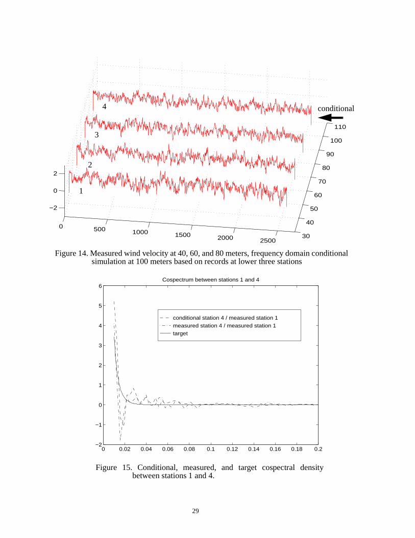
An example application of Gaussian conditional simulation is shown in Figs. 14 and 17.

examples are based on measured correlated wind velocity records at four elevations on a fu

tower with the mean removed. Figure 14 shows three of these records at stations 1 through

frequency domain conditional simulation of the fourth location based on information from the

three known records. Here, Eq. 49 is used for a uni-dimensional multi-variate conditional simu

Figure 15 is a comparison of the target cospectrum with the cospectrum between the m

records at station 1 and 4, and the cospectrum between the conditionally simulated record at s

and the measured record at station 1. The jaggedness of the cospectra in the figure arises

variance inherent in individual realizations. An ensemble average of many simulations resul

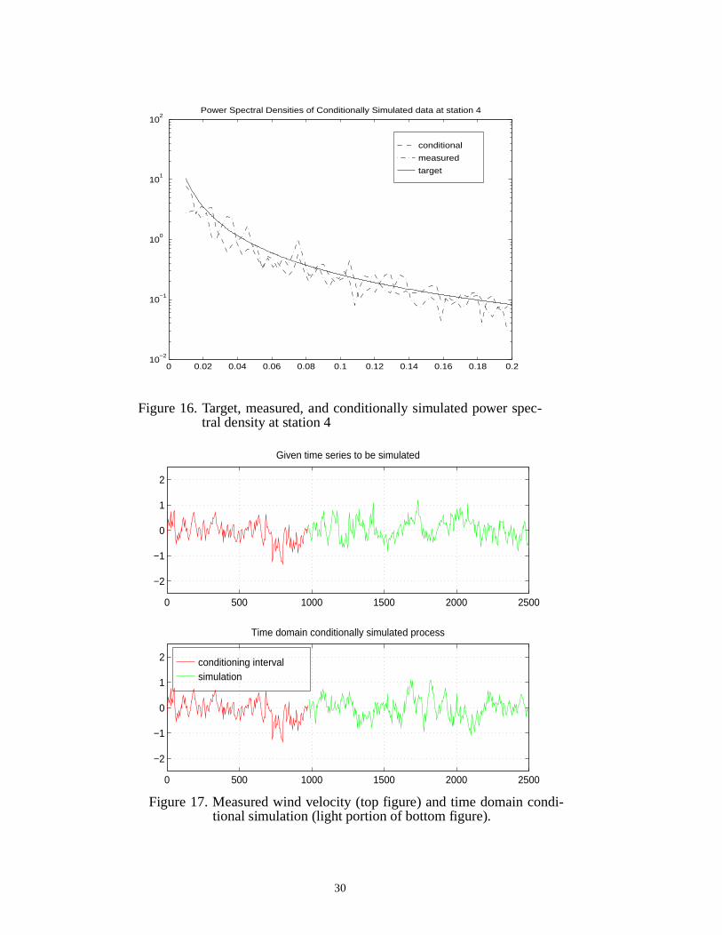
smooth cospectrum which lies along the target cospectrum. Figure 16 is a comparison of th

power spectral density with that from the measured and conditionally simulated records at sta

Figure 17 shows a measured record out to 2500 seconds in the top figure. It is assumed here

record is only available out to 980 seconds, indicated by the darker portion of the signal. A

domain conditional simulation of the record from 980 to 2500 seconds is shown as the lighter

in the bottom figure, based on information from the first 980 seconds. The lighter part of th

figure indicates the portion of this signal which is not known when generating the bottom figure

examples demonstrate the effectiveness and utility of conditional simulation.

In cases involving non-Gaussian processes, the conditional simulation schemes suffer i

ments like their Gaussian counterparts. In Elishakoff et al. (1994), iterative schemes hav

utilized to simulate non-Gaussian processes. The authors sought to combine the techniques d

for unconditional simulation of non-Gaussian processes and the procedure of conditional Ga

processes. The non-Gaussian known processes are mapped into underlying Gaussian p

where conditional simulation is done. These simulated time histories are then mapped back

non-Gaussian domain.

28

l

0 500 1000 1500 2000 250030

40

50

60

70

80

90

100

110

−2

0

2

conditional

1

2

3

4

Figure 14. Measured wind velocity at 40, 60, and 80 meters, frequency domain conditionasimulation at 100 meters based on records at lower three stations

conditional station 4 / measured station 1measured station 4 / measured station 1 target

0 0.02 0.04 0.06 0.08 0.1 0.12 0.14 0.16 0.18 0.2−2

−1

0

1

2

3

4

5

6Cospectrum between stations 1 and 4

Figure 15. Conditional, measured, and target cospectral densitybetween stations 1 and 4.

29

conditional

measured

target

0 0.02 0.04 0.06 0.08 0.1 0.12 0.14 0.16 0.18 0.210

−2

10−1

100

101

102

Power Spectral Densities of Conditionally Simulated data at station 4

Figure 16. Target, measured, and conditionally simulated power spec-tral density at station 4

Figure 17. Measured wind velocity (top figure) and time domain condi-tional simulation (light portion of bottom figure).

conditioning intervalsimulation

0 500 1000 1500 2000 2500

−2

−1

0

1

2

Time domain conditionally simulated process

0 500 1000 1500 2000 2500

−2

−1

0

1

2

Given time series to be simulated

30

WAVEL ET TRANSFORMS

The inability of conventional Fourier analysis to preserve the time dependence and describe

the evolutionary spectral characteristics of nonstationary processes requires tools which allow time

and frequency localization beyond customary Fourier analysis. The short-term Fourier transform

(STFT) provides time and frequency localization to establish a local spectrum for any time instant.

The problem is that high resolution cannot be obtained in both time and frequency domains simulta-

neously. The moving window must be chosen for locating sharp peaks or low frequency features,

because of the inverse relation between window length and the corresponding frequency bandwidth.

This drawback can be alleviated if one has the flexibility to allow the resolution in time and

frequency to vary in the time-frequency plane to reach a multi-resolution representation of the pro-

cess. This is possible if the analysis is viewed as a filter bank consisting of band-pass fil ters with con-

stant relative bandwidths. One type of local transform is the recently developed wavelet transform

(WT) which decomposes a signal using wavelet functions. Fourier methods of signal decomposition

use infinite sines and cosines as basis functions, whereas the wavelet transform uses a set of orthogo-

nal basis functions which are local. Various dilations and translations of a parent wavelet are joined to

form the family of basis functions. This allows the retention of local transient signal characteristics

beyond the capabilities of the harmonic basis functions. The wavelet transform allows a multi-resolu-

tion representation of a process and provides a flexible time-frequency window which narrows to

observe high-frequency energy content, and broadens to capture low frequency phenomena.

Brief Wavelet Overview

Development of the parent wavelet begins with the solution of a dilation equation to determine

a scaling function , dependent on certain restrictions. The scaling function is used to define the

parent wavelet function, . The basis functions used to represent the signal are defined by transla-

tions and dilations of the parent wavelet. The shape of the parent wavelet is not a single unique shape,

but depends on the desired wavelet order.

The signal being decomposed must consist of samples, where is an integer. Wavelet

analysis decomposes the signal into levels, where the level is denoted as , and the levels are

numbered . Each level consists of translated and partially overlapping

wavelets equally spaced intervals apart. The wavelets at level are dilated such that an

individual wavelet spans of that levels intervals, where is the order of the wavelet being

applied. Each of the wavelets at level is scaled by a coefficient determined by the for-

ward wavelet transform, a convolution of the signal with the wavelet. The notation is such that cor-

φ n( )

ψ n( )

2M

M

M 1+ i

i 1 0 1 ...M 1–, , ,–= i j 2i

=

2M

j⁄ j 2i

= i

N 1– N

j 2i

= i ai j,

i

31

n as a

s. The

o per-

ation of

other-

of the

ion. The

domain

rying

well to

ds to a

d and

k. The

ds the

ft block

d-pass

nel or

relative

wn in

er rela-

to first

sonance

ify, e.g.,

ructure,

wind and

either

other

velet

responds to the wavelet dilation, and is the wavelet translation in level . is often writte

vector , where . There are as many wavelet coefficients as signal sample

level is the signal mean value (Newland, 1993). A variety of packages are available t

form discrete wavelet transform (DWT) analysis (e.g. Kareem et al., 1993).

Applications to Wind Engineering

The present research concerns the use of wavelets to aid in the analysis and simul

nonstationary data. Multi-scale decomposition of processes utilizing wavelets reveals events

wise hidden in the original time history. Wavelet coefficients may be used to derive an estimate

power spectrum. These estimates may be extended to multivariate, e.g., cospectral estimat

wavelet coefficients provide the scalogram, which describes the signal energy on a time-scale

over a range of logarithmically spaced frequency bands. This facilitates identification of time-va

energy flux and spectral evolution. The property of accurate energy representation lends itself

signal reconstruction and simulation. A stochastic manipulation of the wavelet coefficients lea

simulation which is statistically similar to the original signal.

Wavelet Filterbank

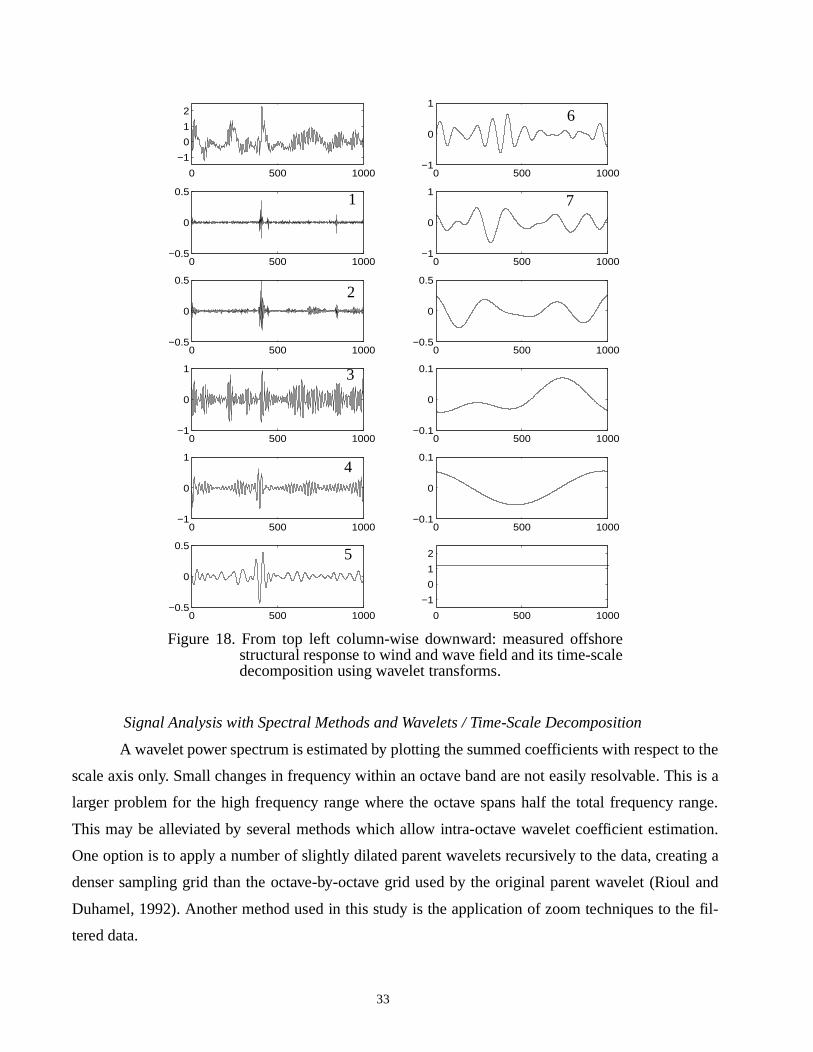
Figure 18 presents the time history of the response of a large floating structure to win

wave loads, and the resulting band-passed time histories using a wavelet based filterban

summation of the band-passed histories returns the original time history. This figure unfol

response time history into a very revealing display of the time-scale representation. The top le

is the mean-removed original signal, the blocks following column-wise downward are the ban

filtered signal in order of decreasing frequency, and the lower right block is the low pass chan

mean of the signal. Note the different scales on the plots for the filtered processes, indicating

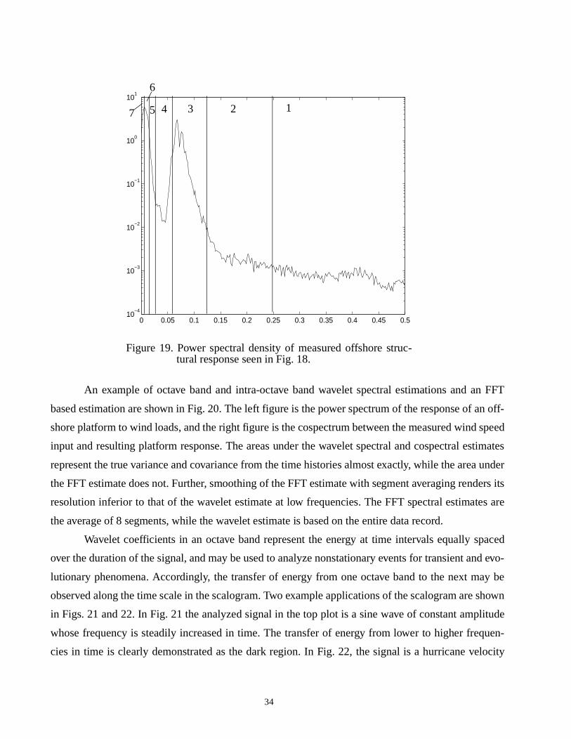
contribution in that frequency band. The power spectral density of the signal in Fig. 18 is sho

Fig. 19, in which the frequency bands 1 through 7 of the filtered process are marked. The high

tive magnitudes of bands 3 and 4 correspond to the right peak in the spectrum, and are due

order wave effects. The high relative magnitude in bands 6 and 7 corresponds to structural re

due to wind and second-order wave effects. The wavelet-based filter bank has helped to ident

high frequency spikes and their time of occurrence, associated with waves slamming the st

observed in bands 1 and 2. These transient events in the response of the structure exposed to

wave fields are not clearly discernible in the time history where large excursions may be due to

occasional slamming, or large but not slamming waves. The improved efficiency over FFT and

filtering techniques, e.g., multifiltering with simple oscillators (e.g., Kameda, 1975), renders wa

filterbanks a quick and convenient time-scale decomposition method.

j i ai j,

a2i j+

j 0 1 ... i 1–, , ,=

i 1–=

32

to the

his is a

range.

ation.

ating a

ul and

the fil-

Signal Analysis with Spectral Methods and Wavelets / Time-Scale Decomposition

A wavelet power spectrum is estimated by plotting the summed coefficients with respect

scale axis only. Small changes in frequency within an octave band are not easily resolvable. T

larger problem for the high frequency range where the octave spans half the total frequency

This may be alleviated by several methods which allow intra-octave wavelet coefficient estim

One option is to apply a number of slightly dilated parent wavelets recursively to the data, cre

denser sampling grid than the octave-by-octave grid used by the original parent wavelet (Rio

Duhamel, 1992). Another method used in this study is the application of zoom techniques to

tered data.

0 500 1000

−1

0

1

2

0 500 1000−1

0

1

0 500 1000−0.5

0

0.5

0 500 1000−1

0

1

0 500 1000−0.5

0

0.5

0 500 1000−0.5

0

0.5

0 500 1000−1

0

1

0 500 1000−0.1

0

0.1

0 500 1000−1

0

1

0 500 1000−0.1

0

0.1

0 500 1000−0.5

0

0.5

0 500 1000

−1

0

1

2

Figure 18. From top left column-wise downward: measured offshorestructural response to wind and wave field and its time-scaledecomposition using wavelet transforms.

1

2

3

4

5

6

7

33

n FFT

f an off-

d speed

stimates

a under

ders its

tes are

spaced

and evo-

ay be

e shown

plitude

quen-

elocity

An example of octave band and intra-octave band wavelet spectral estimations and a

based estimation are shown in Fig. 20. The left figure is the power spectrum of the response o

shore platform to wind loads, and the right figure is the cospectrum between the measured win

input and resulting platform response. The areas under the wavelet spectral and cospectral e

represent the true variance and covariance from the time histories almost exactly, while the are

the FFT estimate does not. Further, smoothing of the FFT estimate with segment averaging ren

resolution inferior to that of the wavelet estimate at low frequencies. The FFT spectral estima

the average of 8 segments, while the wavelet estimate is based on the entire data record.

Wavelet coefficients in an octave band represent the energy at time intervals equally

over the duration of the signal, and may be used to analyze nonstationary events for transient

lutionary phenomena. Accordingly, the transfer of energy from one octave band to the next m

observed along the time scale in the scalogram. Two example applications of the scalogram ar

in Figs. 21 and 22. In Fig. 21 the analyzed signal in the top plot is a sine wave of constant am

whose frequency is steadily increased in time. The transfer of energy from lower to higher fre

cies in time is clearly demonstrated as the dark region. In Fig. 22, the signal is a hurricane v

0 0.05 0.1 0.15 0.2 0.25 0.3 0.35 0.4 0.45 0.510

−4

10−3

10−2

10−1

100

101

Figure 19. Power spectral density of measured offshore struc-tural response seen in Fig. 18.

12345

6

7

34

record measured after the hurricane eye has passed the instrument. In the scalogram the light region

shows the band of frequency content of the record remains relatively constant, while the magnitude at

earlier time is larger than at later time, suggesting nonstationary features.

Wavelet Simulation of Nonstationary Processes

The concept of applying a modulated stationary process centered at narrow-banded frequen-

cies to model ground motion has been extensively used (e.g., Saragoni and Hart, 1974; Li and

Kareem, 1991). In this representation each component process, , is modulated by a different

modulating function

. (50)

There are different approaches to modeling and to describe .

The retention of both time and frequency information makes wavelets a useful tool for the

simulation of nonstationary signals. This can be done given either a parent nonstationary signal, or a

target spectrum and modulator function for each octave. Given a parent nonstationary signal, e.g., a

local wind velocity record, an ensemble of signals may be simulated whose average statistics closely

resemble those of the parent process. The parent signal is discrete wavelet transformed (DWT), and

the coefficients multiplied by a Gaussian white noise of unit variance . The inverse wavelet

transform (IWT) then produces a simulation statistically similar to the parent process.

Given a target spectrum and modulator functions for each octave, the simulation is done by

0 0.002 0.004 0.006 0.008 0.01 0.012 0.014 0.016 0.018 0.020

5

10

15

20

25

0 0.005 0.01 0.015 0.02 0.025 0.03-60

-40

-20

0

20

40

60

Figure 20. Left - Power spectrum estimates of offshore platform response using FFT, octave bandwavelet, and intra-octave band wavelet estimation techniques. Right - cospectrum esti-mates between wind velocity input and resulting platform response.

solid = FFT estimate-o- = octave band wavelet estimate....... = intra-octave band wavelet estimate

sj t( )

mj t( )

x t( ) mj t( )sj t( )j

∑=

mj sj x

w n( )

35

0 2 4 6 8 10 12 14 16 18 20

−1

−0.5

0

0.5

1

time (sec)

fre

qu

en

cy (

Hz)

0 2 4 6 8 10 12 14 16 1810

15

20

25

Figure 21. Frequency modulated sine wave and scalogram

0 10 20 30 40 50 605

10

15

20

25

30

time (sec)

fre

qu

en

cy (

Hz)

0 10 20 30 40 50

8

10

12

14

16

18

Figure 22. Measured hurricane data and scalogram

0

1

36

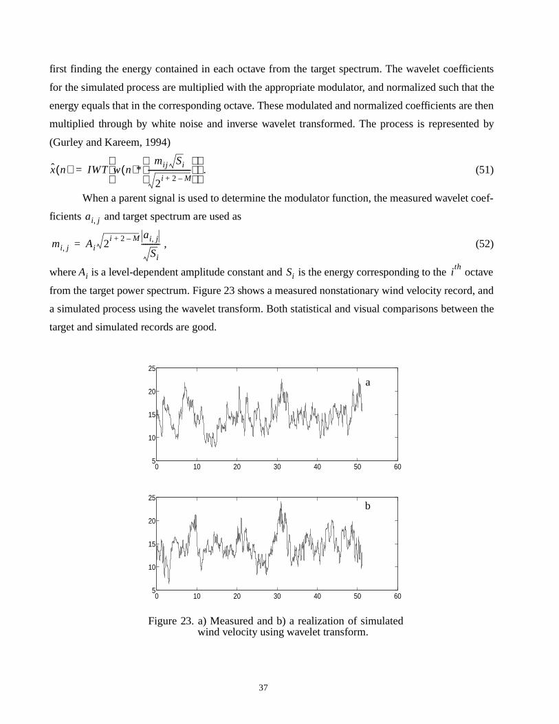
first finding the energy contained in each octave from the target spectrum. The wavelet coefficients

for the simulated process are multiplied with the appropriate modulator, and normalized such that the

energy equals that in the corresponding octave. These modulated and normalized coefficients are then

multiplied through by white noise and inverse wavelet transformed. The process is represented by

(Gurley and Kareem, 1994)

. (51)

When a parent signal is used to determine the modulator function, the measured wavelet coef-

ficients and target spectrum are used as

, (52)

where is a level-dependent amplitude constant and is the energy corresponding to the octave

from the target power spectrum. Figure 23 shows a measured nonstationary wind velocity record, and

a simulated process using the wavelet transform. Both statistical and visual comparisons between the

target and simulated records are good.

x n( ) IWT w n( )*mij Si

2i 2 M–+

-----------------------

=

ai j,

mi j, Ai 2i 2 M–+ ai j,

Si

----------=

Ai Si ith

Figure 23. a) Measured and b) a realization of simulatedwind velocity using wavelet transform.

0 10 20 30 40 50 605

10

15

20

25

0 10 20 30 40 50 605

10

15

20

25

a

b

37

ind on

iew of

f esti-

tion is

onlinear

Volterra

system

r simu-

lterra

plica-

tation of

accom-

s and

223),

artially

y Pro-

, Vol-

, Vol-

orks

Wiley

ll.

CONCLUDING REMARKS

Progress in quantifying and simulating the non-Gaussian and nonstationary effects of w

structures has been elusive due to the limitations of traditional analytical tools. Here, an overv

techniques is presented with examples which aid in the efficient modeling, simulation, and pd

mation of non-Gaussian processes. The estimation of Volterra kernels from system identifica

addressed, as well as other representations for nonlinear systems. The estimated pdf of n

system response is presented via several methods with examples which involve the use of

kernels in the Kac-Siegert approach, the use of joint moment information as constraints on

entropy, and the use of moment-based Hermite transformation models. Several techniques fo

lating non-Gaussian signals, including convolving Fourier amplitude pairs with higher-order Vo

kernels, nonlinear mapping, as well the concept of conditional simulation, are discussed. The im

tions of non-Gaussian winds and their load effects on fatigue damage and gust factor represen

dynamic wind loads are illustrated. The analysis and simulation of nonstationary processes is

plished by the application of localized basis functions via the wavelet transform. Application

examples are given which pertain to nonstationary effects of wind on structures.

ACKNOWLEDGEMENTS

The support for this work was provided in part by NSF Grants BCS-9096274 (BCS-8352

CMS9402196, and ONR Grant N00014-93-1-0761. The first and second authors were p

supported by a Department of Education GAANN Fellowship during this study.

REFERENCES

Ammon, D. (1990), “Approximation and Generation of Gaussian and non-Gaussian Stationarcesses,” Structural Safety, 8: 153-160.

Ang, A. H-S. and Tang, W.H. (1975), Probability Concepts in Engineering Planning & Designume I - Basic Principles. John Wiley & Sons, Inc., New York.

Ang, A. H-S. and Tang, W.H. (1984), Probability Concepts in Engineering Planning & Designume II - Decision, Risk, and Reliability. John Wiley & Sons, Inc., New York.

Antsaklis, P.J. (1993), “Control Theory Approach,” Mathematical Approaches to Neural Netw(ed. J.G. Taylor), Elsevier Science Publishers B.V., 1-23.

Bendat, J.S. (1990), Non-linear System Analysis and Identification from Random Data, Johnand Sons, Inc., New York.

Borgman, L.E. (1990), “Irregular Ocean Waves: Kinematics and Forces,” The Sea, Prentice Ha

38

glassons on9.

Wind

of a

Safe-

cribed

h ap- 28,

ST3)

lewood

Ran-

SCE,

ilizingl Con-s, Am-

l vol-hods

, Ad-

d Eng.

:226-

erna-blish-

Calderone, I., Cheung, J.C.K., and Melbourne, W.H. (1994), “The full-scale significance, oncladding panels, of data obtained from wind tunnel measurements of pressure fluctuatibuilding cladding,” Journal of Wind Engineering and Industrial Aerodynamics, 53: 247-5

Calderone and Melbourne (1993), “The Behavior of Glass Under Wind Loading,” Journal of Engineering and Industrial Aerodynamics, 48: 81-94.

Cartwright, D.E. and Longuet-Higgins, M.S. (1956), “The Statistical Distribution of the MaximaRandom Function,” Proceedings of the Royal Society of London A, Vol. 237, pp. 212-32.

Cheong, H-F. (1995), “Estimation of the minimum pressure coefficient due to gusts,” Structuralty, Elsevier, 17, 1-16.

Conner, D.A. and Hammond, J.L. (1979), “Modeling of Stochastic System Inputs Having PresDistribution and Covariance Functions,” Applied Mathematical Modeling, 3(2).

Davenport, A.G. (1964), “Note on the distribution of the largest value of a random function witplication to gust loading,” Proceedings of the Institution of Civil Engineers London, Vol.pp. 187-96.

Davenport, A.G. (1967), “Gust Loading Factors,” Journal of the Structural Division ASCE, 93(11-34.

Deutsch, R. (1962), Nonlinear Transformations of Random Processes, Prentice-Hall, EngCliffs.

Elishakoff, I., Ren, Y.J. and Shinozuka, M. (1994), “Conditional Simulation of Non-Gaussian dom Fields,” Engineering Structures, 16(7): 558-563.

Grigoriu, M. (1984), “Crossing of Non-Gaussian Translation Process,” J. Engrg. Mech., A110(4): 610-20.

Grigoriu, M. (1995), Applied non-Gaussian Processes, Prentice Hall P T R.

Gurley, K. and Kareem, A. (1994), “On the Analysis and Simulation of Random Processes UtHigher Order Spectra and Wavelet Transforms,” Proceedings of the Second Internationaference on Computational Stochastic Mechanics, Athens, Greece, Balkema Publishersterdam, Netherlands.

Gurley, K. and Kareem, A. (1995), “Simulation of a Class of Non-Normal Processes, “Speciaume of the Journal of Nonlinear Mechanics, EUROMECH-Colloquium No. 329 on Metfor Nonlinear Stochastic Structural Dynamics.

Hertz, J., Krogh, A., and Palmer, R.G. (1991), Introduction to the Theory of Neural Computationdison-Wesley Publishing Company, New York.

Holmes, J.D. (1981), “Non-Gaussian Characteristics of Wind Pressure Fluctuations,” J. of Winand Ind. Aero., 7: 103-108.

Holmes, J.D. (1985), “Wind Action on Glass and Brown’s Integral,” Engineering Structures, 7230.

Hoshiya, M. (1993), “Conditional Simulation of a Stochastic Field,” Proceedings of the 6th Inttional Conference on Structural Safety and Reliability, Innsbruck, Austria. Balkema Puers, Amsterdam, Netherlands.

39

IEEE,

Law

ering

ndom

ns.

nt

ieldspa-

U.S., LA,

essescturals.

onlin-ium on), AS-

g Plat-ME,

teady

trong

f the

g, 14:

nts on

FFT,”

Johnson, G.E. (1994), “Constructions of Particular Random Process,” Proceedings of the82(2): 270-285.

Kac, M. and Siegert, A.J.F. (1947), “On the Theory of Noise in Radio Receivers With SquareDetectors,” J. Applied Physics, Vol. 8, pp. 383-397.

Kameda, H. 1975. “Evolutionary Spectra of Seismogram by Multifilter,” Journal of the enginemechanics division, ASCE. 101(EM6): 787-801.

Kameda, H. and Morikawa, H. (1994), “A Conditioned Stochastic Processes for Conditional RaFields,” Journal of Engineering Mechanics, ASCE, 120(4): 855-875.

Kapur, J.N., (1989), Maximum Entropy Models in Science and Engineering, John Wiley and So

Kareem, A. (1978), “Wind Excited Motion of Tall Buildings,” Ph.D. Dissertation in partial fulfillmeof the degree of doctor of philosophy, Colorado State University, Fort Collins, CO.

Kareem, A. and Li, Y. (1988), “On Modeling The Nonlinear Relationship Between Random FBy Means of Higher-Order Spectra,” Probabilistic Methods in Civil Engineering (P.D. Snos, editor), ASCE, NY, pp. 384-387.

Kareem, A. (1993), “Numerical Simulation of Stochastic Wind effects,” Proceedings of the 7thNational Conference on Wind Engineering, Vol. 1, Wind Engineering Research CouncilCalifornia.

Kareem, A., Gurley, K. and Kantor, J.C. (1993), “Time-Scale Analysis of Nonstationary ProcUtilizing Wavelet Transforms,” Proceedings of the 6th International Conference on StruSafety and Reliability, Innsbruck, Austria, Balkema Publishers, Amsterdam, Netherland

Kareem, A., Hsieh, C.C., Tognarelli, M.A. (1994). “Response analysis of offshore systems to near random waves part I: wave field characteristics,” Proceedings of the special symposstochastic dynamics and reliability of nonlinear ocean systems, Ibrahim and Lin (eds.ME, Chicago, IL, Nov.

Kareem, A. and Zhao, J. (1994), “Analysis of Non-Gaussian Surge Response of Tension Leforms Under Wind Loads,” Journal of Offshore Mechanics and Arctic Engineering, ASVol. 116; 137-144.

Kawai, H. (1983), “Pressure Fluctuations on Square Prisms-Applicability of Strip and Quasi-STheories”, J. of Wind Eng. Ind. Aerodyn., 13:197-208.

Kobayashi, H., Hatanaka, A., and Ueda, T. (1994), “Active Simulation of Time Histories of SWind Gust in a Wind Tunnel,” J of Wind Engineering and Ind. Aero., 53: 315-30.

Krayer, W.R. and Marshall, R.D. (1992), “Gust Factors Applied to Hurricane Winds,” Bulletin oAmerican Meteorological Society, Vol. 73(5): 613-17.

Kung, S.Y. (1993), Digital Neural Networks, PTR Prentice Hall, Englewood Cliffs, New Jersey.

Langley, R.S. (1987), “A statistical Analysis of Non-linear Random Waves,” Ocean Engineerin389-407.

Letchford et al. (1993), “The Application of the Quasi-steady Theory to Full Scale Measuremethe Texas Tech Building,” J. of Wind Eng. Ind. Aerodyn., 48:111-132.

Li. Y. and Kareem, A., (1991), “Simulation of multivariate nonstationary random processes by

40

igital

., En-

ayer of theol. 2.

pro-

ech., Uni-

p Res.,

is ofpro-

ong-

ineer-

” J. of

Water-

f Wind

rans-

ineer-

d non-

ons.

Fluctu-: 623-

Journal of engineering mechanics, ASCE. 117: 1037-1058.

Li. Y. and Kareem, A. (1993). “Simulation of multivariate random processes: Hybrid DFT and dfiltering approach,” Journal of engineering mechanics, ASCE. 119: 1078-98.

Madsen, H.O., Krenk, S. and Lind, N.C. (1986), Methods of Structural Safety. Prentice-Hall, Incglewood Cliffs, N.J.

Maruyama, T. and Marikawa, H. (1995), “Digital Simulation of Wind Fluctuations in Boundary LUsing Experimental Data,” Wind Engineering, Retrospect and Prospect, ProceedingsNinth International Conference on Wind Engineering, New Delhi, India, January 9-13. V

Mignolet, M.P. and Spanos, P.D. (1987), “Recursive simulation of stationary multivariate randomcesses,” Journal of applied mechanics, 54: 674-87.

Murlidharan, T. and Kareem, A. (1993), “Conditional Simulation of Gaussian Velocity Field,” TReport no. CEGEOS-93-1, Department of Civil Engineering and Geological Sciencesversity of Notre Dame.

Naess, A. (1985), “Statistical Analysis of Second-order Response of Marine Structures,” J. Shi29(4): 270-284.

Nam, S.W., Powers, E.J., and Kim, S.B. (1990), “Applications of Digital Polyspectral AnalysNonlinear System Identification,”. Proc. 2nd IASTED international symposium of signal cessing and its applications. Gold Coast, Australia. pp. 133-136.

Newland, D.E. (1993), An Introduction to Random Vibrations, Spectral & Wavelet Analysis. Lman Scientific & Technical, and John Wiley & Sons, New York.

Ochi, M.K. (1986), “Non-Gaussian random processes in ocean engineering,” Probabilistic Enging Mechanics, 1: 28-39.

Peterka, J.A. and Cermak, J.E. (1975), “Wind Pressures on Buildings - Probability Densities,Structural Div., ASCE, 101 (ST6): 1255-67.

Read, W.W., and Sobey, R.J. (1987), “Phase Spectrum of Surface Gravity Waves,” Journal ofway, Port, Coastal, and Ocean Engineering, Vol. 113(5), pp. 507-522.

Reed, D.A. (1993), “Influence of Non-Gaussian Local Pressures on Cladding Glass,” Journal oEngineering and Industrial Aerodynamics, 48:51-61.

Rioul, O., and Duhamel, P. (1992), “Fast Algorithms for Discrete and Continuous Wavelet Tforms,” IEEE Transactions on Information Theory. 38: 569-86.

Saragoni, G.R., and Hart, G.C. (1974), “Simulation of Artificial Earthquakes,” Earthquake Enging Struct. Dyn., 2: 249-267.

Sarkani, S., Kihl, D.P. and Beach, J.E. (1994), “Fatigue of Welded Joints Under NarrowbanGaussian Loadings,” Probabilistic Engineering Mechanics, 9: 179-190.

Schetzen, M. (1980), The Volterra and Wiener Theories of Nonlinear Systems, John Wiley & S

Seong, S.H. and Peterka, J.A. (1993), “Computer Simulation of Non-Gaussian Wind Pressure ations,” Proceedings of the seventh U.S. National Conference on Wind Engineering, 2632.

41

J. of

oba-

Divi-

s, En-

Sys-

The-Colo-

Windonfer-

uake

ering

ds,” J.

Shinozuka, M. (1971), “Simulation of Multivariate and Multidimensional Random Processes,”Acoust. Soc. Am., 49: 357-368.

Sobczyk, K., and Trebicki, J. (1990), “Maximum Entropy Principle in Stochastic Dynamics,” Prbilistic Engineering Mechanics, 5(3): 102-110.

Soize, C. (1978), “Gust Loading Factors with Nonlinear Pressure Terms,” J. of the Structuression, ASCE, Vol. 104(6): 991-1007.

Soong, T.T., and Grigoriu, M. (1993), Random Vibration of Mechanical and Structural Systemglewood Cliffs. N.J., Prentice Hall.

Spanos, P.D. and Donley, M.G. (1991). “Equivalent Statistical Quadratization for Nonlineartems,” Journal of Engineering Mechanics, ASCE, 117(6): 1289-1309.

Tieleman, H.W., and Hajj, M.R. (1995), “Pressures on a Flat Roof-Application of Quasi-Steadyory,” Proceedings of ASCE Specialty Conference, Engineering Mechanics, Boulder, rado.

Thomas, G., Sarkar, P.P. and Mehta, K.C. (1995), “Identification of Admittance Functions for Pressures From Full-Scale Measurements,” Proceedings of the Ninth International Cence on Wind Engineering, New Delhi, India, January 9-13. pp. 1219-1230.

Vanmarcke, E.H. and Fenton, G.A. (1991), “Conditional Simulation of Local Fields of EarthqGround Motion,” Structural Safety, 10: 247-264.

Winterstein, S.R. (1988), “Nonlinear Vibration Models for Extremes and Fatigue,” J. of EngineMechanics, ASCE, 114(10): 1772-1790.

Yamazaki, F. and Shinozuka, M. (1988), “Digital Generation of Non-Gaussian Stochastic Fielof Engineering Mechanics, ASCE, 114(7): 1183-97.

42