Embed Size (px)
Citation preview
NORTHWESTERN UNIVERSITY
Analysis, Characterization and Design of Data Mining Applications
and Applications to Computer Architecture
A DISSERTATION
SUBMITTED TO THE GRADUATE SCHOOL
IN PARTIAL FULFILLMENT OF THE REQUIREMENTS
for the degree
DOCTOR OF PHILOSOPHY
Field of Electrical and Computer Engineering
By
Berkin Ozisikyilmaz
EVANSTON, ILLINOIS
December 2009

2
c© Copyright by Berkin Ozisikyilmaz 2009
All Rights Reserved

3
ABSTRACT
Analysis, Characterization and Design of Data Mining Applications
and Applications to Computer Architecture
Berkin Ozisikyilmaz
Data mining is the process of automatically finding implicit, previously unknown, and
potentially useful information from large volumes of data. Data mining algorithms have
become vital to researchers in science, medicine, business, and security domains. Recent
advances in data extraction techniques have resulted in tremendous increase in the input
data size of data mining applications. Data mining systems, on the other hand, have been
unable to maintain the same rate of growth. Therefore, there is an increasing need to
understand the bottlenecks associated with the execution of these applications in modern
architectures.
In our work, we present MineBench, a publicly available benchmark suite contain-
ing fifteen representative data mining applications belonging to various categories. First,
we highlight the uniqueness of data mining applications. Subsequently, we evaluate the
MineBench applications on an 8-way shared memory (SMP) machine and analyze impor-
tant performance characteristics. Our results show that data mining workloads are quite

4
different than those of other common workloads. Therefore, there is a need to specifically
address the limitations of accelerating them. We propose some initial designs and results
for accelerating them using programmable hardware.
After the analysis of the data mining applications, we have started using them to solve
some of the computer architecture problems. In a study, we have used linear regression
and neural network models in the area of design space exploration area. Design space
exploration is a tedious, complex and time consuming task of determining the optimal
solution to a problem. Our methodology relies on extracting the performance of a small
fraction of the machines to create a model and use it to predict the performance of any
machine. We have also shown using a subset of the processors available for purchase; we
can create a very accurate model presenting the relation between the processor properties
and its price. In another study, we try to achieve the ultimate goal of computer system
design, i.e. satisfy the end-users, using data mining methods. We aim at leveraging the
variation in user expectations and satisfaction relative to the actual hardware performance
to develop more efficient architectures that are customized to end-users.

5
Acknowledgements
I express my deep gratitude to my advisors, Prof. Alok Choudhary, and co-advisor
Prof. Gokhan Memik for their constant guidance and extensive feedback. My gratitude
and appreciation also goes to Prof. Wei-keng Liao for serving as one of the committee
member of my thesis and for his valuable feedback. This work was supported in part by
National Science Foundation (NSF) under grants NGS CNS-0406341, IIS-0536994/002,
CNS-0551639, CCF-0621443, CCF-0546278, and NSF/CARP ST-HEC program under
grant CCF-0444405, and in part by the Department of Energys (DOE) SCiDAC program
(Scientific Data Management Center), number DE-FC02-01ER25485, DOE grants DE-
FG02-05ER25683, and DE-FG02-05ER25691, and in part by Intel Corporation.
I would like to thank my lab mates at Center for Ultra Scale Computing and Informa-
tion Security and Microarchitecture Research Lab at Northwestern University for teaming
with me in realizing my research goals. I would also like to thank my friends for those
lighter moments during my doctoral study at Northwestern.
Last but not least, I am very grateful to my mother Neyran Uzkan and father Ziya
Ozisikyilmaz for their encouragement and moral support through all these years in my
life, and also for providing me the best possible level of education and knowledge. Also,
I would like to thank my brother Ozgun Ozisikyilmaz for his continuous encouragement.

6
Table of Contents
ABSTRACT 3
Acknowledgements 5
List of Tables 9
List of Figures 11
Chapter 1. Introduction 15
1.1. Contributions 18
1.2. Organization 19
Chapter 2. Literature Survey 21
2.1. Analysis, Characterization and Design of Data Mining Applications 21
2.2. Applications of Data Mining to Computer Architecture 24
Chapter 3. MineBench 27
3.1. Need for a New Benchmarking Suite and Uniqueness 28
3.2. Benchmark Suite Overview 31
Chapter 4. Architectural Characterization 41
4.1. Execution Time and Scalability 41
4.2. Memory Hierarchy Behavior 45

7
4.3. Instruction Efficiency 47
Chapter 5. Hardware Acceleration of Data Mining Applications 50
5.1. Kernels 50
5.2. Case Studies using Reconfigurable Accelerator 54
5.3. Case Studies using Graphical Processing Unit as Hardware Accelerator 59
Chapter 6. Embedded Data Mining Workloads 66
6.1. Fixed Point Arithmetic 67
6.2. Selected Applications 68
6.3. Conversion and Results 69
Chapter 7. Data Mining Models to Predict Performance of Computer System
Design Alternatives 75
7.1. Motivation 75
7.2. Overview of Predictive Modeling 77
7.3. Predictive Models 80
7.4. Prediction Results 87
Chapter 8. Profit-Aware Cache Architectures 107
8.1. Speed-binning 107
8.2. Substitute Cache Scheme 109
8.3. Price Modeling 110
8.4. Revenue Estimation and Profit 113

8
Chapter 9. Learning and Leveraging the Relationship between Architecture-Level
Measurements and Individual User Satisfaction 117
9.1. Motivation 117
9.2. Hardware Performance Counters 119
9.3. Experimental Setup 120
9.4. Relation between user Satisfaction and Hardware Performance Counters 120
9.5. Predictive User-Aware Power Management 123
9.6. Predictive Model Building 124
9.7. Experimental Results 127
Chapter 10. Conclusion 131
10.1. Future Work 133
References 135
Appendix A. Training Neural Networks 146
Appendix B. Correlation factors for user satisfaction 150

9
List of Tables
3.1 Overview of the MineBench data mining benchmark suite 27
3.2 Comparison of data mining application with other benchmark
applications 30
4.1 MineBench executable profiles 42
5.1 Top three kernels of applications in MineBench and their contribution
to the total execution time 52
5.2 Basic statistical Kernels 63
6.1 Overview of the MineBench applications analyzed 69
6.2 Timing and Speedup for K-means 70
6.3 Relative Percentage Error for K-means Membership 70
6.4 Timing and Speedup for Fuzzy K-means 72
6.5 Relative Percentage Error for Fuzzy K-means Membership 72
6.6 Timing and Speedup for Utility Mining 73
6.7 Average Relative Error for the total utility values of the points for
various support values 73

10
6.8 Number of Itemsets satisfying the Utility criteria for various support
values 74
7.1 Data statistics obtained from SPEC announcements 89
7.2 Data set obtained from SPEC announcements (32 dimensions/columns) 90
7.3 Configurations used in microprocessor study 92
7.4 Data statistics obtained from SPEC benchmark simulations 92
7.5 Average accuracy results from SPEC published results 104
7.6 The best accuracy achieved for single processor and multiprocessor
chronological design space exploration and the model that achieves
this accuracy 105
7.7 Average accuracy results from SPEC simulations 106
8.1 Increase in revenue for various cache-architectures 115
9.1 Hardware counters we use in our experiments 120
B.1 Correlation between the hardware performance counters and user
satisfaction 150

11
List of Figures
1.1 Data mining applications in MineBench 17
3.1 Classification of data mining, SPEC INT, SPEC FP, MediaBench
and TPC-H benchmark applications based on their characteristics. A
K-means based clustering algorithm was used for this classification.
Data mining applications tend to form unique clusters. 30
4.1 Speedups for the MineBench applications 43
4.2 L1 Data Miss Rates 45
4.3 L2 Cache Miss Rates 45
4.4 Branch Misprediction Rate 48
4.5 Fraction of Floating Point Instructions 48
4.6 Resource Related Stalls 48
4.7 Instructions Per Cycle 48
5.1 Speedups for the MineBench applications 51
5.2 Data Mining Systems Architecture 53
5.3 Design of the Reconfigurable Data Mining Kernel Accelerator 53
5.4 Distance calculation kernel 55
12
5.5 Minimum computation kernel 55
5.6 Architecture for Decision Tree Classification 59
5.7 GPU vs. CPU Floating-Point Performance 60
5.8 GeForce 8800 GPU Hardware showing Thread Batching 61
5.9 Performance results for basic statistical functions for different input
size 64
6.1 Fixed Point Conversion Methodology 67
7.1 Overview of design space exploration using predictive modeling: (a)
sampled design space exploration and (b) chronological predictive
models. 79
7.2 Multiple Layered ANN 84
7.3 An example of a hidden unit 84
7.4 Estimated vs. true error rates for Opteron based systems 93
7.5 Estimated vs. true error rates for Opteron 2 based systems 94
7.6 Estimated vs. true error rates for Pentium 4 based systems 95
7.7 Estimated vs. true error rates for Pentium D based systems 96
7.8 Estimated vs. true error rates for Xeon based systems 96
7.9 Chronological predictions for Xeon (a), Pentium 4 (b), Pentium D (c)
based systems 99

13
7.10 Chronological predictions for Opteron based multiprocessor systems:
(a) one processor, (b) two processors, (c) four processors, and (d)
eight processors 99
7.11 Estimated vs. true error rates for Applu application: NN-E (L), NN-S
(M), LR-B (R) 102
7.12 Estimated vs. true error rates for Equake application: NN-E (L),
NN-S (M), LR-B (R) 102
7.13 Estimated vs. true error rates for Gcc application: NN-E (L), NN-S
(M), LR-B (R) 103
7.14 Estimated vs. true error rates for Mcf application: NN-E (L), NN-S
(M), LR-B (R) 103
7.15 Estimated vs. true error rates for Mesa application: NN-E (L), NN-S
(M), LR-B (R) 103
8.1 (a) Frequency binning in modern microprocessors. (b) Price vs.
frequency of Intel Pentium 4 family 108
8.2 Binning with (a) 5-bin and (b) 6-bin strategy for SC- 4 and SC-8
schemes 114
9.1 Framework of the predictive user-aware power management 124
9.2 User satisfaction and dynamic power reduction for iDVFS over
Windows XP DVFS scheme. In the graphs, the horizontal axes reflect
the individual users in the study, while the left vertical axes reflect

14
the reported satisfaction for iDVFS and Windows XP DVFS, and the
right vertical axes report the percentage reduction in dynamic power
of iDVFS compared to Windows XP DVFS 126
9.3 Improvement in energy consumption, user satisfaction, and
energy-satisfaction product for the Shockwave application 129

15
CHAPTER 1
Introduction
Latest trends indicate beginning of a new era in data analysis and information ex-
traction. Todays connect anytime and anywhere society based on the use of digital tech-
nologies is fueling data growth, which is doubling every two years (if not faster), akin to
“Moore’s law for data” [52]. This growth is transforming the way business, science and
digital technology based world function. Various businesses are collecting vast amounts
of data to make forecasts and intelligent decisions about future directions. The worlds
largest commercial databases are over the 100TB mark, whereas the database sizes on
hybrid systems are approaching the PB mark [111]. Some of these large databases are
growing by a factor of 20 every year. In addition, millions of users on the Internet are
making data available for others to access. Countless libraries and databases containing
photographs, movies, songs, etc. are available to a common user. In addition to the
increasing amount of available data, other factors make the problem of information ex-
traction particularly complicated. First, users ask for more information to be extracted
from their data sets, which requires increasingly complicated algorithms. Second, in many
cases, the analysis needs to be done in real time to reap the actual benefits. For instance,
a security expert would strive for real-time analysis of the streaming video and audio
data in conjunction. Managing and performing run-time analysis on such data sets is
appearing to be the next big challenge in computing.

16
For these reasons, there is an increasing need for automated applications and tools to
extract the required information and to locate the necessary data objects. Data mining
is the process of automated extraction of predictive information from large datasets.
It involves algorithms and computations from different domains such as mathematics,
machine learning, statistics, and databases. Data mining is becoming an essential tool
in various fields including business (marketing, fraud detection, credit scoring, decision
systems), science (climate modeling, astrophysics, biotechnology), and others such as
search engines, security, and video analysis.
An important perspective on applications and workloads for future data intensive ap-
plications is Recognition, Mining, and Synthesis [19]. In this perspective, applications are
divided into three groups; namely, Recognition, Mining and Synthesis (RMS). Recogni-
tion (R) is the capability to recognize or learn interesting patterns or a model within large
amounts of data for a specific application domain. Patterns may be of interest in het-
erogeneous applications such as video surveillance, credit card and banking transactions,
security related databases with government agencies etc.. Mining (M) is the capability
to analyze these large amounts of data for important objects or events, knowledge or
actionable items. Depending on the type of applications domain, different characteristics
and outcomes dominate. For example, for intrusion detection or on-line surveillance, the
ability to continuously mine real-time streams of data is very important, whereas for a
health-care diagnosis and personalized medicine application, accurate prediction of dis-
ease and treatment based on historical data and models would be important. Recognition
and Mining are closely related. Finally, Synthesis (S) refers to applications that can use
these models and data to create virtual or artificial environments to mimic the patterns

17
Figure 1.1. Data mining applications in MineBench
that are discovered. Alternatively, these models and outcomes may be incorporated into
operational systems of businesses, such as recommendation systems for health-care or
marketing. Clearly, these characteristics are quite different from traditional IT applica-
tions, which are targeted by current hardware and software systems. Just as graphics and
multimedia applications have had tremendous impact on processors and systems, these
data intensive data mining applications are expected to have tremendous impact on future
systems.
Data mining applications are classified based on the methodology used for data analy-
sis and information learning. A typical data mining taxonomy is shown in Figure 1.1 [47].
Note that the same data can be analyzed using different techniques. For instance, a mobile
phone company can use clustering mechanisms to identify the current traffic distribution
before reassigning base stations. On the other hand, an analyst would use predictive
methods to identify potential customers for a new mobile phone service plan. In addi-
tion, a data mining application usually consists of sequential execution of a number of
tasks/algorithms. For example, a data set might first be pre-processed (e.g., sorted), then
clustered, and then analyzed using association rule discovery.

18
Recently, more and more computer architecture researchers are borrowing machine
learning / data mining techniques to attack problems in real-world computer systems:
such as modeling microprocessors [61] and cache structures, power and performance
modeling of applications [66, 115], reduced workloads and traces to decrease simulation
time [32, 56]. The motivation is simple: building empirical models based on statisti-
cal pattern recognition, data mining, probabilistic reasoning and other machine learning
methods promises to help us cope with the challenges of scale and complexity of current
and future systems. In the following sections, we present some other applications of data
mining algorithms in computer architecture.
1.1. Contributions
In this thesis, we do analysis and performance characterization of data mining appli-
cations and then show how we can borrow ideas from this domain to tackle and solve
computer architecture related problems. In particular, we make following contributions:
• We have shown that data creation and collection rates are growing exponentially.
Data mining is becoming an important tool used by researchers in many domains.
Previously, there hasn’t been a mechanism to review data mining algorithms and
the systems that run them. Therefore we have introduced, NU-MineBench, a
data mining benchmark suite.
• Initial analysis has shown that data mining applications have significantly dif-
ferent characteristics than previously available benchmarks such as SPEC, i.e.

19
data mining applications are both data and computation intensive. Since cur-
rent architectures are designed for the older workloads, we have done detailed
architectural characterization to find the needs of data mining applications.
• We have proposed how we can use reconfigurable and reprogrammable hardwares
to overcome some of the bottlenecks identified in the characterization phase.
These results indicate that significant performance improvement can be achieved.
Also we have shown that conversion of floating point operations to fixed point
operations on these reconfigurable architectures can further increase the perfor-
mance.
• The problems in the computer architecture area are very large, complex and time
consuming to solve. We have presented how we can use some basic data mining
methods and applied them to these problems. Specifically, we have shown that
the efforts needed to solve the design space exploration problem can be reduced as
much as 100× without causing significant impact on the accuracy of the solution.
We have also applied these ideas to areas where previous computer architecture
researches have mostly neglected: a) the revenue and profit implications of design
decisions b) the user satisfaction during the runtime of an application.
1.2. Organization
The rest of the dissertation continues as follows: Chapter 2 provides related work
in the area of benchmarking, data mining and applications of data mining to computer
architecture research. First, in Chapter 3 we show why we need a new benchmarking suit
and then introduce the MineBench benchmark in detail. Then Chapter 4 describes the

20
architectural characteristics of the benchmark for single and multiprocessor cases. Opti-
mization of data mining workloads using hardware accelerators are presented in Chapter
5. Chapter 6 continues with our related work in the embedded data mining systems
area. Chapter 7 shows an example of how data mining applications can be used to tackle
the complex design space problem in computer architecture. Then, data mining models
are used to present the strong relation between the processor properties and its price in
Chapter 8. Chapter 9 is the last example where data mining was used to learn per user
satisfaction for different applications and leverage it to save power. Our conclusion is
presented in Chapter 10 and followed by future work.

21
CHAPTER 2
Literature Survey
Benchmarks play a major role in all domains. SPEC [103] benchmarks have been well
accepted and used by several chip makers and researchers to measure the effectiveness
of their designs. Other fields have popular benchmarking suites designed for the specific
application domain: TPC [107] for database systems, SPLASH [113] for parallel archi-
tectures, and MediaBench [67] for media and communication processors. We understand
the indispensable need for a data mining benchmark suite since there are currently no
mechanisms to review data mining algorithms and the systems that run them.
2.1. Analysis, Characterization and Design of Data Mining Applications
Performance characterization studies similar to ours have been previously performed
for database workloads [48, 62], with some of these efforts specifically targeting SMP
machines [92, 106]. Performance characterization of individual data mining algorithms
have been done [20, 64], where the authors focus on the memory and cache behavior of
a decision tree induction program.
Characterization and optimization of data-mining workloads is a relatively new field.
Our work builds on prior effort in analyzing the performance scalability of bioinformat-
ics workloads performed by researchers at Intel Corporation [26]. As it will be de-
scribed in the following Chapter 3, we incorporate their bioinformatics workloads into

22
our MineBench suite, and where applicable, make direct comparisons between their re-
sults and our own. However, MineBench is more generic and covers a wider spectrum
than the bioinformatics applications previously studied [26]. Jaleel et al. examine the
last-level cache performance of these bioinfomatics applications [58].
The bioinformatics applications presented in MineBench differ from other recently-
developed bioinformatics benchmark suites. BioInfoMark [68], BioBench [3], BioSplash [9],
and BioPerf [8] all contain several applications in common, including Blast, FASTA,
Clustalw, and Hmmer. BioInfoMark and BioBench contain only serial workloads. In
BioPerf, a few applications have been parallelized, unlike MineBench which contains full
fledged OpenMP [18] parallelized codes of all bioinformatics workloads. Srinivasan et
al. [102] explore the effects of cache misses and algorithmic optimizations on performance
for one of the applications in MineBench (SVM-RFE), while our work investigates several
architectural features of data mining applications. Sanchez et al. [94] perform architec-
tural analysis of a commonly used biological sequence alignment algorithm, whereas we
attempt to characterize a variety of data mining algorithms used in biological applications.
There has been prior research on hardware implementations of data mining algo-
rithms. In [35] and [112], K-means clustering is implemented using reconfigurable hard-
ware. Baker and Prasanna [11] use FPGAs to implement and accelerate the Apriori [2]
algorithm, a popular association rule mining technique. They develop a scalable systolic
array architecture to efficiently carry out the set operations, and use a “systolic injec-
tion” method for efficiently reporting unpredicted results to a controller. In [10], the
same authors use a bitmapped CAM architecture implementation on an FPGA platform
to achieve significant speedups over software implementations of the Apriori algorithm.

23
Compared to our designs, these implementations target different classes of data mining al-
gorithms. We have also looked at Graphical Processing Units (GPUs) as the new medium
of hardware acceleration. Barrachina et al. [14, 13] evaluate the performance of Level 3
operations in CUBLAS. They also present algorithms to compute the solution of a linear
system of equations on a GPU, as well as general techniques to improve their performance.
Jung [57] presents an efficient algorithm for solving symmetric and positive definite linear
systems using the GPU. Govindaraju et al. [45] present algorithms for performing fast
computation of several common database operations, e.g., conjugate selections, aggrega-
tions, and semi-linear queries, on commodity graphics hardware. Volkov [109] presents
dense linear algebra and Nukada et. al. [82] present 3-D FFT on NVIDIA GPUs. As
these studies show that GPUs can be used for various application domains, they do not
specifically focus on data mining algorithms, which is the target of our work.
Our approach in the embedded data mining work is similar to work done in the Digital
Signal Processing [75, 93] domain. In [93], the authors have used MATLAB to semi-
automate conversion of floating point MATLAB programs into fixed point programs, to
be mapped onto FPGA hardware. Their implementation tries to minimize hardware
resources, while constraining quantization errors within a specific limit. Currently our
fixed point conversion is done manually. However, we support varying precisions and do
not perform input scaling transformations. In [24], an implementation of sensory stream
data mining using fixed point arithmetic has been described. The authors in [40] have
used fixed point arithmetic with pre-scaling to obtain decent speedups for artificial neural
networks used in natural language processing. Several data mining algorithms have been
previously implemented on FPGAs [12, 118, 36, 24]. In [12], the Apriori algorithm,
24
which is nearly pure integer arithmetic, has been implemented on hardware. In [36],
algorithmic transformations on K-means clustering have been studied for reconfigurable
logic. In [65], the authors have implemented Basic Local Alignment Search Tool (BLAST)
by using a low level FPGA near the disk drives, and then using a traditional processor.
2.2. Applications of Data Mining to Computer Architecture
There have been numerous works done in the area of design space exploration. Ey-
erman et al. [37] uses a different heuristics to model the shape of the design space of
superscalar out-of-order processor. Ipek et al. [55] use artificial neural networks to pre-
dict the performance of memory, processor, and CMP design spaces. However, in their
work, they have only used simulation results to create their design space for SPEC2000
applications, and used neural networks with cross validation to calculate their prediction
accuracy. Meanwhile, Lee et al. [66] use regression models to predict performance and
power usage of the applications found in the SPECjbb and SPEC2000 benchmarks. As
in the previous reference, the data points are created using simulations. Kahn et al. [63]
uses predictive modeling, a machine learning technique to tackle the problem of accu-
rately predicting the behavior of unseen configurations in CMP environment. Ghosh et
al. [42] have presented an analytical approach to the design space exploration of caches
that avoids exhaustive simulation. Their approach uses an analytical model of the cache
combined with algorithms to directly and efficiently compute a cache configuration meet-
ing designers’ performance constraints. The problem that they are trying to solve (only
varying cache size and associativity) is very small compared to the ones that other re-
searchers and we are trying to solve. Dubach et al. [31] has used a combination of linear

25
regressor models in conjunction with neural networks to create a model that can predict
the performance of programs on any microarchitectural configuration with only using 32
further simulations. In our work, we target system performance rather than processor
performance. All of these works have based their models on simulation while our results
use simulation results as well as already built existing computer systems. The closest work
is by Ipek et al. [54], where they use artificial neural networks to predict the performance
of SMG2000 applications run on multi-processor systems. The application inputs and the
number of processors the application runs on are changed during their analysis. Their
accuracy results are around 12.3% when they have 250 data points for training. However,
we must point that they also do not perform an estimation of the performance of the
systems but rather simulate the execution of an application on one system.
Variability in process technologies, that we have based our work Profit-Aware Cache
Architecture, has been extensively studied. There have been several cache redundancy
schemes proposed. These techniques have been/could be used to reduce the critical delay
of a cache. Victim caches [60] are extra level of caches used to hold blocks evicted from a
CPU cache due to a conflict or capacity miss. A substitute cache (SC) storing the slower
blocks of the cache is orthogonal to a victim cache, which stores blocks evicted from the
cache. Sohi [99] shows that cache redundancy can be used to prevent yield loss, using a
similar concept to our proposed SC cache. Ozdemir et al. [87] present microarchitectural
schemes that improve the overall chip yield under process variations. The authors have
shown how powering down sections of the cache can increase the effective yield. Our work,
on the other hand encompasses extra redundancy in L1 caches to facilitate efficient binning
and profit maximization. There have been numerous studies analyzing cache resizing for

26
different goals such as minimizing power consumption or increasing performance. Selective
Cache Ways by Albonessi [4] is one of the first works in cache resizing and optimizing
energy dissipation of the cache. However, to the best of our knowledge no resizing schemes
has been applied to alter speed-binning and profit.
Dynamic voltage and frequency scaling (DVFS) is an effective technique for micropro-
cessor energy and power control for most modern processors [21, 44]. Energy efficiency
has traditionally been a major concern for mobile computers. Fei, Zhong and Ya [39]
propose an energy-aware dynamic software management framework that improves bat-
tery utilization for mobile computers. However, this technique is only applicable to highly
adaptive mobile applications. Researchers have proposed algorithms based on workload
decomposition [27], but these tend to provide power improvements only for memory-
bound applications. Wu et al. [114] present a design framework for a run-time DVFS
optimizer in a general dynamic compilation system. However, none of the previous DVFS
techniques consider the user satisfaction prediction. Mallik et al. [73, 74] show that it
is possible to utilize user feedback to control a power management scheme, i.e., allow the
user to control the performance of the processor directly. However, their system requires
constant feedback from the user. Our scheme, correlates to user satisfaction with low
level microarchitectural metrics. In addition, we use a learning mechanism to eliminate
the user feedback to make long-term feedback unnecessary. Sasaki et al. [95] propose a
novel DVFS method based on statistical analysis of performance counters. However, their
technique needs compiler support to insert code for performance prediction. Furthermore,
their technique does not consider user satisfaction while setting the frequency.

27
CHAPTER 3
MineBench
The increasing performance gap between data mining systems and algorithms may be
bridged by a two phased approach: a thorough understanding of the system character-
istics and bottlenecks of data mining applications, followed by design of novel computer
Table 3.1. Overview of the MineBench data mining benchmark suite
Application Category Description
ScalParC Classification Decision tree classificationNaive Bayesian Classification Simple statistical classifier
K-means Clustering Mean-based data partitioning methodFuzzy K-means Clustering Fuzzy logic-based data partitioning method
HOP Clustering Density-based grouping methodBIRCH Clustering Hierarchical clustering method
Eclat ARMVertical database, Lattice transversal
techniques used
Apriori ARMHorizontal database, level-wise mining based on
Apriori propertyUtility ARM Utility-based association rule mining
SNP ClassificationHill-climbing search method for DNA
dependency extraction
GeneNet ClassificationGene relationship extraction using
microarray-based method
SEMPHY ClassificationGene sequencing using phylogenetic tree-based
method
Rsearch ClassificationRNA sequence search using stochastic Context-Free
Grammars
SVM-RFE ClassificationGene expression classifier using recursive feature
elimination
PLSA OptimizationDNA sequence alignment using Smith-Waterman
optimization method

28
systems to cater to the primary demands of data mining workloads. We address this
issue in this work by investigating the execution of data mining applications on a shared-
memory parallel (SMP) machine. We first establish a benchmarking suite of applications
that we call MineBench, which encompasses many algorithms commonly found in data
mining. We then analyze the architectural properties of these applications to investigate
the performance bottlenecks associated with them. The fifteen applications that currently
comprise MineBench are listed in Table 3.1, and are described in more detail in Section
3.2.
3.1. Need for a New Benchmarking Suite and Uniqueness
A new benchmarking suite is highly motivated if applications in a domain exhibit
distinctive characteristics. In this section, we focus on the uniqueness of data mining
applications, as compared to other application domains. We compare the architectural
characteristics of applications across various benchmark suites. Specifically, data mining
applications are compared against compute intensive applications, multimedia applica-
tions, streaming applications and database applications to identify the core differences.
In this analysis, we used a variety of application suites including integer application bench-
marks (SPEC INT from SPEC CPU2000 [103]), floating point application benchmarks
(SPEC FP from SPEC CPU2000), multimedia application benchmarks (MediaBench [67])
and decision support application benchmarks (TPC-H from Transaction Processing Coun-
cil [107]). We perform statistical analysis on 19 architectural characteristics (such as
branch instructions retired, L1 and L2 cache accesses, etc.) of the applications and use
this information to identify the core differences. Specifically, we monitor the performance

29
counters of each application during execution using profiling tools, and obtain their in-
dividual characteristics. The experimental framework is identical to the one described
in Chapter 4. The applications are then categorized using a K-means based approach,
which clusters the applications with similar characteristics together. A similar approach
has been used to identify a representative workload of SPEC benchmarks [33]. Figure 3.1
shows the scatter plot of the final configuration obtained from the results of the clustering
method. Applications belonging to the SPEC INT, SPEC FP, TPC-H, and MediaBench
benchmark suites are assigned to respective clusters. However, it can be seen that data
mining applications stand out from other benchmark suites: they are scattered across sev-
eral clusters. Although some of the data mining applications share characteristics with
other application domains, they mostly exhibit unique characteristics. Another important
property of the clustering results is the large variation within data mining applications.
Although most of the applications in other benchmarking suites fall into one cluster, data
mining applications fall into seven different clusters. This shows the large variation of
characteristics observed in data mining applications. Overall, this analysis highlights the
need for a data mining benchmark consisting of various representative algorithms that
cover the spectrum of data mining application domains.
Table 3.2 shows the distinct architectural characteristics of data mining applications as
compared to other applications. One key attribute that signifies the uniqueness of data
mining applications is the number of data references per instruction retired. For data
mining applications, this rate is 1.103, whereas for other applications, it is significantly
less. The number of bus accesses originating from the processor to the memory (per

30
0
1
2
3
4
5
6
7
8
9
gcc
bzip
2
gzip
mcf
twol
f
vort
ex vpr
pars
er
apsi art
equa
ke
luca
s
mes
a
mgr
id
swim
wup
wis
e
raw
caud
io
epic
enco
de
cjep
g
mpe
g2
pegw
it gs
toas
t
Q17 Q3
Q4
Q6
aprio
ri
baye
sian
birc
h
ecla
t
hop
scal
parc
kMea
ns
fuzz
y kM
eans
rsea
rch
sem
phy
snp
gene
net
svm
-rfe
Clu
ster
#
SPEC INT SPEC FP MediaBench TPC-H Data Mining
Figure 3.1. Classification of data mining, SPEC INT, SPEC FP, Media-Bench and TPC-H benchmark applications based on their characteristics.A K-means based clustering algorithm was used for this classification. Datamining applications tend to form unique clusters.
Table 3.2. Comparison of data mining application with other benchmark applications
Benchmark of ApplicationsParameter† SPECINT SPECFP MediaBench TPC-H NU-MineBench
Data References 0.81 0.55 0.56 0.48 1.10Bus Accesses 0.030 0.034 0.002 0.010 0.037
Instruction Decodes 1.17 1.02 1.28 1.08 0.78Resource Related Stalls 0.66 1.04 0.14 0.69 0.43
CPI 1.43 1.66 1.16 1.36 1.54ALU Operations 0.25 0.29 0.27 0.30 0.31
L1 Misses 0.023 0.008 0.010 0.029 0.016L2 Misses 0.003 0.003 0.0004 0.002 0.006Branches 0.13 0.03 0.16 0.11 0.14
Branch Mispredictions 0.009 0.0008 0.016 0.0006 0.006† The numbers shown here for the parameters are values per instruction
instruction retired) verify the frequency of data access of data mining applications. These
results solidify the intuition that data mining is data-intensive by nature.
The L2 miss rates are considerably high for data mining applications. The reason for
this is the inherent streaming nature of data retrieval, which does not provide enough
opportunities for data reuse. This indicates that current memory hierarchy is insufficient

31
for data mining applications. It should be noted that the number of branch instructions
(and the branch mispredictions) are typically low for data mining applications, which
highlights yet another unique behavior of data mining applications.
Another important difference is the fraction of total instruction decodes to the in-
structions retired. This measure identifies the instruction efficiency of a processor. In
our case, the results indicate that data mining applications are efficiently handled by the
processor. The reason for this value being less than one is the use of complex SSE2 in-
structions. Resource related stalls comprises of the delay that incurs from the contention
of various processor resources, which include register renaming buffer entries, memory
buffer entries, and also the penalty that occurs during a branch misprediction recovery.
The number of ALU operations per instruction retired is also surprisingly high for data
mining applications, which indicates the extensive amount of computations performed in
data mining applications. Therefore, data mining applications are computation-intensive
in addition to being data-intensive.
What makes the data mining applications unique is this combination of high data rates
combined with high computation power requirements. Such a behavior is clearly not seen
in other benchmark suites. In addition, data mining applications tend to oscillate between
data and compute phases, making the current processors and architectural optimizations
mostly inadequate.
3.2. Benchmark Suite Overview
MineBench contains fifteen representative data mining workloads from various cat-
egories. The workloads chosen represent the heterogeneity of algorithms and methods

32
used in data mining. Applications from clustering, classification, association rule mining
and optimization categories are included in MineBench. The codes are full fledged im-
plementations of entire data mining applications, as opposed to stand-alone algorithmic
kernels. We provide OpenMP parallelized codes for twelve of the fifteen applications. An
important aspect of data mining applications are the data sets used. For most of the
applications, we provide three categories of data sets with varying sizes: small, medium,
and large. In addition, we provide source code, information for compiling the applications
using various compilers, and command line arguments for all of the applications.
3.2.1. Classification Workloads
A classification problem has an input dataset called the training set, which consists of
example records with a number of attributes. The objective of a classification algorithm
is to use this training dataset to build a model such that the model can be used to assign
unclassified records into one of the defined classes [47].
ScalParC is an efficient and scalable variation of decision tree classification [59]. The
decision tree model is built by recursively splitting the training dataset based on an
optimality criterion until all records belonging to each of the partitions bear the same class
label. Decision tree based models are relatively inexpensive to construct, easy to interpret
and easy to integrate with commercial database systems. ScalParC uses a parallel hashing
paradigm to achieve scalability during the splitting phase. This approach makes it scalable
in both runtime and memory requirements.
The Naive Bayesian classifier [30], a simple statistical classifier, uses an input training
dataset to build a predictive model (containing classes of records) such that the model can

33
be used to assign unclassified records into one of the defined classes. Naive Bayes classifiers
are based on probability models that incorporate strong independence assumptions which
often have no bearing in reality, hence the term “naive”. They exhibit high accuracy and
speed when applied to large databases.
Single nucleotide polymorphisms (SNPs), are DNA sequence variations that occur
when a single nucleotide is altered in a genome sequence. Understanding the importance
of the many recently identified SNPs in human genes has become a primary goal of human
genetics. The SNP [26] benchmark uses the hill climbing search method, which selects
an initial starting point (an initial Bayesian Network structure) and searches that point’s
nearest neighbors. The neighbor that has the highest score is then made the new current
point. This procedure iterates until it reaches a local maximum score.
Recent advances in DNA microarray technologies have made it possible to measure
expression patterns of all the genes in an organism, thereby necessitating algorithms that
are able to handle thousands of variables simultaneously. By representing each gene as a
variable of a Bayesian Network (BN), the gene expression data analysis problem can be
formulated as a BN structure learning problem. GeneNet [26] uses a similar hill climbing
algorithm as in SNP, the main difference being that the input data is more complex,
requiring much additional computation during the learning process. Moreover, unlike the
SNP application, the number of variables runs into thousands, but only hundreds of train-
ing cases are available. GeneNet has been parallelized using a node level parallelization
paradigm, where in each step, the nodes of the BN are distributed to different processors.
SEMPHY [26] is a structure learning algorithm that is based on phylogenetic trees.
Phylogenetic trees represent the genetic relationship of a species, with closely related

34
species placed in nearby branches. Phylogenetic tree inference is a high performance
computing problem as biological data size increases exponentially. SEMPHY uses the
structural expectation maximization algorithm, to efficiently search for maximum like-
lihood phylogenetic trees. The computation in SEMPHY scales quadratically with the
input data size, necessitating parallelization. The computation intensive kernels in the
algorithm are identified and parallelized using OpenMP.
Typically, RNA sequencing problems involve searching the gene database for homolo-
gous RNA sequences. Rsearch [26] uses a grammar-based approach to achieve this goal.
Stochastic context-free grammars are used to build and represent a single RNA sequence,
and a local alignment algorithm is used to search the database for homologous RNAs.
Rsearch is parallelized using a dynamic load-balancing mechanism based on partition-
ing the variable length database sequence to fixed length chunks, with specific domain
knowledge.
SVM-RFE [26], or Support Vector Machines - Recursive Feature Elimination, is a
feature selection method. SVM-RFE is used extensively in disease finding (gene expression
problem). The selection is obtained by a recursive feature elimination process - at each
RFE step, a gene is discarded from the active variables of a SVM classification model,
according to some support criteria. Vector multiplication is the computation intensive
kernel of SVM-RFE, and data parallelism using OpenMP, is utilized to parallelize the
algorithm.

35
3.2.2. Clustering Workloads
Clustering is the process of discovering the groups of similar objects from a database to
characterize the underlying data distribution [47]. It has wide applications in market or
customer segmentation, pattern recognition, and spatial data analysis.
The first clustering application in MineBench is K-means [71]. K-means represents a
cluster by the mean value of all objects contained in it. Given the user-provided parameter
k, the initial k cluster centers are randomly selected from the database. Then, each
object is assigned a nearest cluster center based on a similarity function. Once the new
assignments are completed, new centers are found by finding the mean of all the objects
in each cluster. This process is repeated until some convergence criteria is met. K-means
tries to minimize the total intra-cluster variance.
The clusters provided by the K-means algorithm are sometimes called “hard” clusters,
since any data object either is or is not a member of a particular cluster. The Fuzzy K-
means algorithm [16] relaxes this condition by assuming that a data object can have
a degree of membership in each cluster. Compared to the similarity function used in
K-means, the calculation for fuzzy membership results in a higher computational cost.
However, the flexibility of assigning objects to multiple clusters might be necessary to
generate better clustering qualities. Both K-means and Fuzzy K-means are parallelized
by distributing the input objects among the processors. At the end of each iteration,
extra communication is necessary to synchronize the clustering process.
HOP [34], originally proposed in astrophysics, is a typical density-based clustering
method. After assigning an estimation of the density for each particle, HOP associates
each particle with its densest neighbor. The assignment process continues until the densest

36
neighbor of a particle is itself. All particles reaching the same such particle are clustered
into the same group. The advantage of HOP over other density based clustering methods
is that it is spatially adaptive, coordinate-free and numerically straightforward. HOP is
parallelized using a three dimensional KD tree data structure, which allows each thread to
process only a subset of the particles, thereby reducing communication cost significantly.
BIRCH [119] is an incremental and hierarchical clustering algorithm for large databases.
It employs a hierarchical tree to represent the closeness of data objects. BIRCH scans the
database to build a clustering-feature (CF) tree to summarize the cluster representation.
For a large database, BIRCH can achieve good performance and scalability. It is also ef-
fective for incremental clustering of incoming data objects, or when an input data stream
has to be clustered.
3.2.3. ARM Workloads
The goal of Association Rule Mining (ARM) is to find interesting relationships hidden
in large data sets. More specifically, it attempts to find the set of all subsets of items
or attributes that frequently occur in database records [47]. In addition, the uncovered
relationships can be represented in the form of association rules, which state how a given
subset of items influence the presence of another subset.
Apriori [2] is the first ARM algorithm that pioneered the use of support-based pruning
to systematically control the exponential growth of the search space. It is a level-wise
algorithm that employs a generate-and-test strategy for finding frequent itemsets. It is
based on the property that all non-empty subsets of a frequent itemset must all be frequent
(the so-called “Apriori” property). For determining frequent items in a fast manner, the
algorithm uses a hash tree to store candidate itemsets. Note: This hash tree has item sets

37
at the leaves and hash tables at internal nodes. The Apriori algorithm is parallelized by
distributing chunks of the input data among the processors. The master processor then
gathers the local candidate itemsets, and generates globally frequent itemsets.
Utility mining [69] is another association rule-based mining technique where the as-
sumption of uniformity among items is discarded. Higher “utility” itemsets are identified
from a database by considering different values for individual items. The goal of utility
mining is to restrict the size of the candidate set so as to simplify the total number of
computations required to calculate the value of items. It uses the “transaction-weighted
downward closure property” to prune the search space. The parallelization paradigm
applied to Utility mining is the same as in Apriori, described above.
Eclat [116] uses a vertical database format. It can determine the support of any k-
itemset by simply intersecting the id-list of the first two (k-1)-length subsets that share
a common prefix. It breaks the search space into small, independent, and manageable
chunks. Efficient lattice traversal techniques are used to identify all the true maximal
frequent itemsets.
3.2.4. Optimization Workloads
Sequence alignment is an important problem in bioinformatics used to align DNA, RNA
or protein primary sequences so as to emphasize their regions of similarity. It is used
to identify the similar and diverged regions between two sequences, which may indicate
functional and evolutionary relationships between them. PLSA [26] uses a dynamic pro-
gramming approach to solve this sequence matching problem. It is based on the algorithm
proposed by Smith and Waterman, which uses the local alignment to find the longest com-
mon substring in sequences. PLSA uses special data structures to intelligently segment the

38
whole sequence alignment problem into several independent subproblems, which dramat-
ically reduce the computation necessary, thus providing more parallelism than previous
sequence alignment algorithms.
3.2.5. Input Datasets
Input data is an integral part of data mining applications. The data used in our experi-
ments are either real-world data obtained from various fields or widely-accepted synthetic
data generated using existing tools that are used in scientific and statistical simulations.
During evaluation, multiple data sizes were used to investigate the characteristics of the
MineBench applications. For the non-bioinformatics applications, the input datasets were
classified into three different sizes: small, medium, and large. For the ScalParC and Naive
Bayesian applications, three synthetic datasets were generated by the IBM Quest data
generator [1]. Apriori also uses three synthetic datasets from the IBM Quest data gener-
ator with a varying number of transactions, average transaction size, and average size of
the maximal large itemsets. For HOP and Birch, three sets of real data were extracted
from a cosmology application, ENZO [81], each having 61440 particles, 491520 particles
and 3932160 particles.
A section of the real image database distributed by Corel Corporation is used for
K-means and Fuzzy K-means. This database consists of 17695 scenery pictures. Each
picture is represented by two features: color and edge. The color feature is a vector of 9
floating points while the edge feature is a vector of size 18. Since the clustering quality of
K-means methods highly depends on the input parameter k, both K-means were executed
with 10 different k values ranging from 4 to 13.

39
Utility mining uses both real as well as synthetic datasets. The synthetic data consists
of two databases generated using the IBM Quest data generator. The first synthetic
dataset is a dense database, where the average transaction size is 10; the other is a
relatively sparse database, where average transaction size is 20. The average size of the
potentially frequent itemsets is 6 in both sets of databases. In both sets of databases, the
number of transactions varies from 1000K to 8000K and the number of items varies from
1K to 8K. The real dataset consists of only one database of size 73MB, where the average
transaction length is 7.2.
Bioinformatics applications use datasets obtained from different biological databases.
For the bioinformatics applications, the datasets were provided by Intel [26]. SNP uses
the Human Genic Bi-Alletic Sequences (HGBASE) database [22] containing 616,179 SNPs
sequences. For GeneNet, the microarray data used for this study is assembled from [100];
they are the most popular cell cycle data of Yeast. SEMPHY considers three datasets
from the Pfam database [15]. The software and the corresponding dataset for Rsearch
were obtained from [96]. The experiments use the sequence mir-40.stk with the length
of 97 to search a part of database Yeastdb.fa with size of 100KB. SVM-RFE uses a
benchmark microarray dataset on ovarian cancer [5]. This dataset contains 253 (tissue
samples) × 15154 (genes) expression values, including 91 control and 162 ovarian cancer
tissues with early stage cancer samples. For PLSA, nucleotides ranging in length from
30K to 900K are chosen as test sequences. Since true sequences can seldom satisfy this
specific size, some artificial sequences were used in the experiments [26]. To make the
experiments more comprehensive, several real DNA sequences were also chosen from a
test suite provided by the bioinformatics group at Penn State University. The longest

40
sequence pair used here is named TCR where the human sequence is 319,030 bp long and
the mouse sequence is 305,636 bp long.

41
CHAPTER 4
Architectural Characterization
In this section, we consider the applications in our MineBench suite, and distinguish
the characteristics that make each application unique from both the algorithmic and
the system perspective. We chose an Intel IA-32 multiprocessor platform for evaluation
purposes. Our setup consists of an Intel Xeon 8-way Shared Memory Parallel (SMP)
machine running Red Hat Advanced Server 2.1. The system has 4 GB of shared memory.
Each processor has a 16 KB non-blocking, integrated L1 cache and a 1024 KB L2 cache.
For our experiments, we use the VTune Performance Analyzer [53] for profiling the
functions within our applications, and for measuring the execution times. Using the
VTune counters, we monitor a wide assortment of performance metrics: execution time,
communication and synchronization complexity, memory behavior, and Instructions per
Cycle (IPC) statistics. Each application was compiled with version 7.1 of the Intel C++
compiler for Linux.
4.1. Execution Time and Scalability
In Table 4.1, we present the total number of instructions executed across all proces-
sors along with the size of the executables. We can see that these benchmarks execute
from tens of billions to thousands of billions of instructions. As the number of processors
increases, the number of instructions executed is expected to increase due to the overhead
of parallelization (locks, communication, synchronization etc.). However we observe that

42
Table 4.1. MineBench executable profiles
ApplicationInstruction Count (billions)
Size (kB)1 Processor 2 Processors 4 Processors 8 Processors
ScalParC 23.664 24.817 25.550 27.283 154Naive Bayesian 23.981 N/A N/A N/A 207
K-means 53.776 54.269 59.243 77.026 154Fuzzy K-means 447.039 450.930 477.659 564.280 154
HOP 30.297 26.920 26.007 26.902 211BIRCH 15.180 N/A N/A N/A 609
Apriori 42.328 42.608 43.720 47.182 847Eclat 15.643 N/A N/A N/A 2169
Utility 13.460 19.902 20.757 22.473 853SNP 429.703 299.960 267.596 241.680 14016
GeneNet 2,244.470 2,263.410 2,307.663 2,415.428 13636SEMPHY 2,344.533 2,396.901 1,966.273 2,049.658 7991Rsearch 1,825.317 1,811.043 1,789.055 1,772.200 676SVM-RFE 51.370 55.249 63.053 82.385 1336PLSA 4,460.823 4,526.160 4,080.610 4,001.675 836
in some of the applications, instructions retired decreases as the number of processors
increases. This may happen when the convergence criteria is reached at an earlier stage
during execution of the parallel application. In our study, the usage of Vtune Perfor-
mance Analyzer enables us to examine the characteristics of program execution across all
execution phases, something that would not be feasible using simulation for applications
of this size.
Figure 4.1 shows the benchmark application execution speedups when running on
multiple processors. The performance numbers for the 2-processor case shows some trivial
performance improvement for clustering and ARM workloads, while most of the remaining
workloads perform slightly better or worse than the serial case. On the other hand, several
benchmarks show good scalability with higher number of processors. When running on
8 processors, ScalParC executes 4.84 and 5.64× faster than the 1 processor case for the

43
SVM-RFE
0.0
1.0
2.0
3.0
4.0
5.0
6.0
7.0
8.0
1 2 4 8
Number of Processors
Rel
ativ
e S
peed
up
M
PLSA
0.0
1.0
2.0
3.0
4.0
5.0
6.0
7.0
8.0
1 2 4 8
Number of Processors
Rel
ativ
e S
peed
up
SML
Semphy
0.0
1.0
2.0
3.0
4.0
5.0
6.0
7.0
8.0
1 2 4 8
Number of Processors
Rel
ativ
e S
peed
up
SML
Rsearch
0.0
1.0
2.0
3.0
4.0
5.0
6.0
7.0
8.0
1 2 4 8
Number of Processors
Rel
ativ
e S
peed
up
SL
SNP
0.0
1.0
2.0
3.0
4.0
5.0
6.0
7.0
8.0
1 2 4 8
Number of Processors
Rel
ativ
e S
peed
up M
Genenet
0.0
1.0
2.0
3.0
4.0
5.0
6.0
7.0
8.0
1 2 4 8Number of Processors
Rel
ativ
e S
peed
up
M
k-Means
0.0
1.0
2.0
3.0
4.0
5.0
6.0
7.0
8.0
1 2 4 8
Number of Processors
Rel
ativ
e S
peed
up SML
Fuzzy k-Means
0.0
1.0
2.0
3.0
4.0
5.0
6.0
7.0
8.0
1 2 4 8
Number of Processors
Rel
ativ
e S
peed
up
SML
HOP
0.0
1.0
2.0
3.0
4.0
5.0
6.0
7.0
8.0
1 2 4 8
Number of Processors
Rel
ativ
e Sp
eedu
p SML
Apriori
0.0
1.0
2.0
3.0
4.0
5.0
6.0
7.0
8.0
1 2 4 8
Number of Processors
Rel
ativ
e S
peed
up SML
ScalParC
0.0
1.0
2.0
3.0
4.0
5.0
6.0
7.0
8.0
1 2 4 8
Number of Processors
Rel
ativ
e Sp
eedu
p SML
Utility
0.0
1.0
2.0
3.0
4.0
5.0
6.0
7.0
8.0
1 2 4 8
Number of Processors
Rel
ativ
e S
peed
up
SL
Figure 4.1. Speedups for the MineBench applications
small and large data sets, respectively. The best speedup, 7.55x on 8 processors, is seen in
Utility. In this algorithm, data is uniformly distributed to the 8 processors, which are able
to work concurrently by accessing only its respective data block in memory, synchronizing
only occasionally. Rsearch and K-means follow Utility in terms of achieved speedups. In
general, it can be observed that clustering algorithms show better scalability than the
remainder of the applications. The underlying reason for this observation is the highly
parallelizable distance calculation routine, which is common to the clustering algorithms.

44
The worst scalability is observed for SNP and SVM-RFE. For SVM-RFE, the problem
arises due to unnecessary communication problems and locking of memory structures.
This redundant locking is done to ensure the code works on distributed and shared memory
machines.
For the Utility mining application, the small dataset represents real data collected from
a grocery store. The large dataset has been created by the IBM Quest data generator.
Both of the datasets contain a nearly equal number of transactions and items. However,
the speedups for these two datasets differ widely. Particularly, the application achieves
7.55x speed-up for the small and 2.23x speed-up for the large datasets when executed
on 8 processors. When the most time consuming functions are examined, it is seen that
the program spends approximately 30% and 50% of the total execution time in the serial
database read function, respectively. The change in the time of this serial segment causes
the scalability problems for the large dataset.
Intel researchers have done similar analysis for the performance scalability of the bioin-
formatics workloads [26]. When the above presented results are compared to their results,
Genenet, Semphy, Rsearch, and PLSA show very similar scalability trends. However the
results are very different for SNP and SVM-RFE, where they are able to achieve close to
linear speedup until 8 processors and super-linear speedup for 16 processors. The expla-
nation given for this super-linearity is that Intel’s system is composed of a 16-way shared
memory machine, which has a large L3 cache and Cell-sharing L4 caches (4 processors
grouped together) that are interconnected with each other through the crossbar. Specific
optimizations have been applied to these codes targeting their system. However, other
researchers from Intel have shown that SVM-RFE reaches only 2.3x speed-up on their

45
0
2
4
6
8
10
12
14
16
scalp
arc
k-mea
nsfuzz
yho
p
aprio
riutilit
ysn
p
gene
net
semph
y
rsea
rch
svm-rf
epls
a
baye
sian
birch
eclat
Mis
s R
ate
(%)
p=1
p=2
p=4
p=8
Figure 4.2. L1 Data Miss Rates
0102030405060708090
100
scalp
arc
k-mea
nsfuzz
yho
p
aprio
riutilit
ysn
p
gene
net
semph
y
rsea
rch
svm-rf
epls
a
baye
sian
birch
eclat
Mis
s R
ate
(%)
p=1
p=2
p=4
p=8
Figure 4.3. L2 Cache Miss Rates
4-way shared memory machine [102]. This is a sign that architecture plays an important
role in the performance of these applications.
4.2. Memory Hierarchy Behavior
It is well known that memory hierarchy is a major performance bottleneck in modern
computing systems. It is therefore necessary to understand the memory hierarchy behav-
ior of data mining applications before attempting to improve performance. Figures 4.2
and 4.3 summarize the results obtained for memory hierarchy behavior (level 1 data, and
level 2 caches, respectively) over 1, 2, 4 and 8 processor runs on medium sized datasets,
wherever applicable. We notice several interesting aspects of memory behavior from these
results. First, though L1 data cache miss rates are usually small, applications are drasti-
cally different in their L1 data cache behavior. We can separate the applications into two
categories: those that have very small L1 data miss rates (less than 1.5%), and those that
have larger miss rates (2-14%). It is also interesting to note that even in applications with
low L1 data miss rates, in many cases, the 2-processor run yields much higher cache misses
than the other runs. In general, we see that as the number of processors increase, L1 data

46
cache miss rates decrease. This is due to the fact that multiple processors are working on
a smaller chunk of data. Note that, for some applications, the miss rates are independent
of the number of processors. In these applications, most misses are caused by cold and
invalidation misses, hence they are largely unaffected by the number of processors. We
also studied the L1 instruction cache miss rates. In general the L1 instruction cache miss
rates are very low (on average 0.11%). This is due to the fact that the applications are
relatively small in size and the instructions are able to fit into the L1 cache easily. More
importantly, most of the execution in these applications are in the relatively small number
of frequently executed kernels. Since the miss rates during the execution of these kernels
are low, the overall instruction cache misses remain low. We have not observed much
variance of instruction miss rate while going from 1 processors to 8 processors, because
these applications, in general, use data parallelization concepts.
An analysis of the L2 cache behavior was also carried out and yielded several unique
characteristics. It is seen that L2 cache miss rates are many times greater than their
corresponding L1 counterparts. Generally, there are two reasons for such high L2 miss
rates. First, for some applications the L1 miss rates are extremely small, as a result
most of the L2 accesses result in cold misses. Second, several applications work on very
large datasets in a streaming fashion. Overall, the SVM-RFE benchmark had the worst
L2 cache miss rates. Combined with its low L1 efficiency, approximately 8.44% of all
data references incur costly off-chip memory access, thus yielding a very low IPC for this
application. Another interesting observation is that in majority of the applications, the
L2 miss rate for the 2 processor case is highest. One reason for this kind of behavior is
that the data distribution is random as dynamic scheduling is used for parallelization in

47
some of the applications. In dynamic schemes, the processor gets assigned a new block
of data in a random fashion as it becomes available. Hence the data gets distributed
to multiple caches in a random fashion, which increases the likelihood of not exploiting
temporal or spatial data locality.
4.3. Instruction Efficiency
We also studied the instruction efficiency using the counters profiled by VTune. Par-
ticularly, we measure the branch misprediction rates, the fraction of floating-point instruc-
tions, resource related stalls (stalls caused by register renaming buffer entries, memory
buffer entries, and branch misprediction recovery), and the Instructions per Cycle (IPC)
values observed. These results are summarized in Figures 4.4, 4.5, 4.6, and 4.7, respec-
tively.
In general, the branch prediction performs very well, with an average misprediction
rate of 3.27% for the 15 applications. This is mostly due to the fact that the applications
have small kernels which consist of loops that execute for very large number of iterations.
Also, the applications are parallelized using OpenMP, which is good at analyzing large
loops to extract data parallelism in an efficient way. The highest branch misprediction
rate is observed for the HOP and Apriori applications. In both cases, this is partly due
to the paradigm applied to parallelize the algorithms. In these two applications, the
dataset is read in parallel and each processor works on local data for the most part,
only synchronizing occasionally. The application does not have a concise kernel that is
executed repeatedly, hence the branch misprediction increases. It is also seen that, in
most applications, the branch misprediction rate decreases as the degree of parallelism
increases.

48
0
2
4
6
8
10
12
14
16
scalp
arc
k-mea
nsfuzz
yho
p
aprio
riutilit
ysn
p
gene
net
semph
y
rsea
rch
svm-rf
epls
a
baye
sian
birch
eclat
Mis
s R
ate
(%) p=1
p=2
p=4
p=8
Figure 4.4. Branch Mispre-diction Rate
0
5
10
15
20
25
30
35
scalp
arc
k-m
eans
fuzz
yho
p
aprio
riutilit
ysn
p
gene
net
semph
y
rsea
rch
svm-rf
epls
a
baye
sian
birch
eclat
FP
Op
s(%
) p=1
p=2
p=4
p=8
Figure 4.5. Fraction of Float-ing Point Instructions
0102030405060708090
100
scalp
arc
k-m
eans
fuzz
yho
p
aprio
riutilit
ysn
p
gene
net
semph
y
rsea
rch
svm-rf
epls
a
baye
sian
birch
eclat
RR
Sta
lls
(%) p=1
p=2
p=4
p=8
Figure 4.6. Resource Related Stalls
0
0.2
0.4
0.6
0.8
1
1.2
1.4
scalp
arc
k-m
eans
fuzz
yho
p
aprio
riutilit
ysn
p
gene
net
semph
y
rsea
rch
svm-rf
epls
a
baye
sian
birch
eclat
Av
g IP
C
p=1
p=2
p=4
p=8
Figure 4.7. Instructions Per Cycle
We also looked at the percentage of floating point operations performed by the appli-
cations. The results are presented in Figure 4.5. Several of the MineBench applications
are floating point intensive. As the degree of parallelism increases, it is seen that the
percentage of floating point operations decreases (the number of floating point operations
are usually about the same across different number of processors, but the number of in-
structions retired increases, thereby reducing the fraction of FP operations). Note that
Apriori, GeneNet and PLSA are integer applications and do not contain any floating point
operations.

49
Figure 4.6 presents the resource related stall rates for each application. It is seen that
most applications suffer from high stall rates. Particularly, the SVM-RFE application
spends 92% of its execution time on stalls. Since this application exhibits high L1 data
and L2 cache miss rates, the instructions spend more time in the pipeline, which causes
an increase in the resource related stalls. In general, we also observe a correlation between
the number of floating point instructions and resource related stalls. As the fraction of
floating point operations increase, the processor is able to utilize its resources better and
stalls less. However, this is not true for applications like Utility mining and SVM-RFE,
where other effects like large cache miss rates result in higher stall rates. As the number of
processors increase, in general, the resource related stalls increase. For some applications,
this causes the limitation of the scalability we observe, which is described in Section 4.1.
To express the efficiency of data mining applications, the number of Instructions per
Cycle (IPC) has been studied. It can be seen that some applications suffer from very low
IPCs. For example, the SVM-RFE application sees an IPC value of 0.09 with 8 processors.
The reason for such low IPCs are different: SVM-RFE and SNP’s low IPCs are related
to the high resource related stall percentages, 92% and 72% respectively; SVM-RFE,
ScalparC and Utility are affected by high L1 data cache miss rates; Hop and Apriori, on
the other hand, suffer from high branch mispredictions. Also, in almost all applications,
as the degree of parallelism increases, the IPC decreases. In many applications, the
2-processor case experiences the worst IPC results. These results indicate that there
is significant room to improve the performance of the applications by increasing their
efficiencies. The parallelization of these applications also needs to be looked into, since
the applications suffer from various drawbacks as the degree of parallelism increases.

50
CHAPTER 5
Hardware Acceleration of Data Mining Applications
In the beginning of our work we have mentioned that there is a gap between data-
intensive applications and computing systems. In our studies we applied a two-phased
approach: (a) The first phase involves performing an in-depth study to clearly under-
stand the system characteristics and bottlenecks, and also to enlist the future computing
requirements of data mining applications (b) The second phase consists of designing novel
(or adapting existing) computer systems to cater to the primary demands of data mining
workloads. On the other hand, the algorithms too have to be revised to suit the demands
of new applications and architectures. We have explored the first phase in the previous
section and now look into second phase.
Reconfigurable hardware acceleration is an attractive method for the second phase.
In this section we describe a generic data mining system architecture which can be cus-
tomized for specific applications. We also present designs and results for accelerating two
sample applications using programmable hardware. We have also looked how we can use
the ample processing power available in the graphical processing unit.
5.1. Kernels
Data mining applications have several similarities with streaming applications since
a consistently changing set of data is read for processing. But they are different from
pure streaming applications by the fact that there are bursts of streaming data instead of

51
Figure 5.1. Speedups for the MineBench applications
data arriving at a consistent arrival rate. Figure 5.1 shows a generic data flow in such an
application. These applications, therefore, can be characterized as multiphase, with each
phase consisting of one or more kernels. These kernels form pieces of core operations,
e.g., histogram, distance calculation, correlations, tree-search, etc.. These phases repeat
many times, and the data that is consumed in each phase may change their execution
characteristics. In other words, kernel is defined to be an abstract representation of a set
of operations that are performed frequently in an application. Here, we try to extract the
kernels in data mining applications in our quest for understanding their nature. Extraction
of such kernels also helps in identifying how the kernel actually maps to the underlying
architecture components including the processor, memory and other resources.
We have extracted the top 3 kernels for the applications in MineBench. The results
can be seen in Table 5.1. For each application, the name of the kernel and the percentage
of the system time spent executing the kernel are presented. In general, we see that
most applications spend a majority of their time in small concise kernels. Identifying

52
Table 5.1. Top three kernels of applications in MineBench and their contri-bution to the total execution time
ApplicationTop 3 Kernels (%)
Sum[%]Kernel 1 (%) Kernel 2 (%) Kernel 3 (%)
K-means distance (68%) clustering (21%) minDist (10%) 99Fuzzy K-means clustering (58%) distance (39%) fuzzySum (1%) 98
BIRCH distance (54%) variance (22%) redistribution (10%) 86HOP density (39%) search (30%) gather (23%) 92
Naive Bayesian probCal (49%) varience (38%) dataRead(10%) 97ScalParC classify (37%) giniCalc (36%) compare (24%) 97Apriori subset (58%) dataRead (14%) increment (8%) 80Utility dataRead (46%) subsequence (29%) Main (23%) 98
SNP compScore (68%) updateScore (20%) familyScore (2%) 90GeneNet condProb (55%) updateScore (31%) familyScore (9%) 95SEMPHY bestBrnchLen (59%) expectation (39%) lenOpt(1%) 99Rsearch covariance (90%) histogram (6%) dbRead (3%) 99SVM-RFE quotMatrx (57%) quadGrad (38%) quotUpdate (2%) 97PLSA pathGridAssgn (51%)fillGridCache (34%)backPathFind (14%) 99
these kernels can lead to an understanding of the problems in the underlying hardware
architectural components (i.e. processor, memory hierarchy, and other resources).
The results from our previous work [90] show that data mining applications have
hit the performance wall of existing computing systems. In related areas of computing
such as networks, graphics and physics processing, researchers have designed highly opti-
mized architectures for their respective applications. Designing customized systems with
high-speed data mining engines can help alleviate the performance degradation seen in
conventional data mining applications.
In Figure 5.2, we present our generic design of the proposed data mining system
architecture. In this system, we have the reconfigurable data mining accelerator as a
co-processor that communicates with the general purpose processor. In this model, the
processor can send the kernel operations to the accelerator (which executes the kernels

53
Figure 5.2. Data Mining Sys-tems Architecture
Figure 5.3. Design of theReconfigurable Data MiningKernel Accelerator
faster than the processor) and the processor can continue with other non-kernel tasks. In
Figure 5.3, we present details of the accelerator. In this model, when applications are
loaded, their specific kernels should be loaded into the reconfigurable logic. Once the
logics have been loaded, the execution unit hardly needs to be reprogrammed. This is
due to the fact that the kernels remain the same for a given application. Only during
an application change, the execution unit needs to be reprogrammed. The kernels for
the applications are stored in the configuration memory, and their loading is triggered
by the general purpose processor. Once the kernels are identified for each application,
the hardware logic can be built and stored into the configuration memory by examining
the underlying computations. The key to the efficient execution in this model is the
implementation of the kernels. In the following section, we discuss a few examples where
we design efficient architectures for these kernels.

54
5.2. Case Studies using Reconfigurable Accelerator
5.2.1. K-means and Fuzzy K-means
K-means is a clustering algorithm that represents a cluster by the mean value of all
objects contained in it. Given the user-provided parameter k, the initial k cluster centers
are randomly selected from the database. Then, each object is assigned a nearest cluster
based on a similarity function. Once the new assignments are completed, new centers are
found by finding the mean of all the objects in each cluster. This process is repeated until
some convergence criteria is met. In K-means, the “distance” kernel is responsible for
calculating the Euclidean distance between two points and “minDist” kernel calculates
the minimum of the distances. The “clustering” kernel assigns the actual cluster and
recalculates the centers (mean of points in a cluster) in each iteration. Fuzzy K-means
is closely related to K-means, hence the distance calculation appears to be a prominent
kernel for this application as well. In this case, the difference is that the clustering
kernel is more time consuming than the distance calculation. This is because in fuzzy
logic, the computations involved in performing the membership calculation (owing to
multiple membership property) are more intense than the actual distance calculation.
The “fuzzySum” kernel is used during the convergence process. Figure 5.4 and Figure 5.5
show the hardware logic needed to implement the distance and minimum calculations
respectively. The distance calculation logic, uses a level of N subtractors followed by a set
of N multipliers. The third level has a depth of log(N) and contains N-1 cumulative adders.
The minimum computation involves a combination of multiplexers and comparator logic
to compare and send the actual data item to the final level. In these designs the levels
are tightly pipelined, allowing the results to be produced every cycle.

55
Figure 5.4. Distance calcula-tion kernel
Figure 5.5. Minimum compu-tation kernel
In the simulation of these designs, the accelerator has been attached to the overall pro-
cessor, and we use an architecture-level cycle accurate simulator to measure the execution
time. To enable the core processor to offload the kernel computations to the accelera-
tor, markers have been attached in the actual application code. In our results, we have
defined a new total cycle metric which contains the cycles spent by the core processor
in non-kernel parts of the code including the handoff of computations to the accelerator
plus the cycles the accelerator uses to calculate the results. We have tested our design
with datasets of various sizes, and we have observed that as data set size increases, the
speedups improve. This shows that the pipelined design becomes more effective when
data set size increases, and shows that general purpose processors are not able to handle
such streaming data efficiently. For K-means and Fuzzy K-means, we have seen speedups
from 500× to 3600× and 400× to 1600× in the distance calculation kernel, respectively,

56
and 600× to 1600× in minimum kernel in Fuzzy K-means. In the tests, the number of
hardware resources have been varied, and it is clearly seen that application speedups scale
well showing the applications exploit all the parallelism available to them. Overall, we
have seen 11× to 80× speedup for K-means and Fuzzy K-means applications, respectively.
The relatively lower speedups for the applications come from the fact that, when kernels
are accelerated, the non-kernel parts of the applications become more dominant.
5.2.2. Decision Tree Classification
An important problem in data mining is Classification, which is the task of assigning
objects to one of several predefined categories. A classification problem has an input
dataset called the training set, which consists of a number of records, each possessing
multiple attributes. Attributes may be categorical or continuous, depending on whether
they have a discrete or continuous domain. The classifying attribute or class ID is a
categorical attribute, whose value is known for records in the training dataset. A solution
to the classification problem entails developing a model that allows prediction of the class
of a record when the remaining attributes are known. Among existing solutions, Decision
Tree Classification (DTC) is a popular method that yields high accuracy while handling
large datasets. Poor scalability with increasingly large and complex data sets, as well as
the existence of concise, well defined kernels make DTC a suitable candidate for hardware
acceleration.
A decision tree model consists of internal nodes and leaves. Each of the internal nodes
has a splitting decision and a splitting attribute associated with it. The leaves have a class
label assigned to them. Building a decision tree model from a training dataset involves
two phases. In the first phase, a splitting attribute and split index are chosen. The second

57
phase uses this information to distribute records among the child nodes. This process is
recursively continued until a stopping criterion is met. At this point, the decision tree
can be used to predict the class of an incoming record, whose class ID is unknown. The
prediction process is relatively straightforward: the classification process begins at the
root, and a path to a leaf is traced by using the splitting decision at each internal node.
The class label attached to the leaf is then assigned to the incoming record.
Determining the split attribute and the split index is a critical component of the
decision tree induction process. In various optimized implementations of decision tree
induction [97, 59], the splitting criteria used is to minimize the Gini index of the split.
Previous section has shown that the largest fraction of the execution time of representative
implementations is spent in the split determining phase [117]. For example, ScalParC,
which uses a parallel hashing paradigm to efficiently map record IDs to nodes, spends
over 40% of its time in the Gini calculation phase.
In our design of a hardware accelerator for DTC, we have chosen to accelerate the Gini
score computation process. The Gini score is a mathematical measure of the inequality of
a distribution. Computing the gini value for a particular split index requires computing
the frequency of each class in each of the partitions. Therefore a linear search is made for
the optimum split value, by evaluating the Gini score for all possible splits. This process is
repeated for each attribute, and the optimum split index over all attributes is chosen. The
total complexity of this operation is O(|R| ∗ |A|), where |R| and |A| represent the number
of records and the number of attributes, respectively. Our architecture for acceleration
DTC consists of several computation modules, referred to as “Gini Units”, that perform
Gini calculation for a single attribute. The high-level DTC architecture is presented in

58
Figure 5.6. There is a DTC controller component that interfaces with the software and
supplies the appropriate data and signals to the Gini units. The architecture functions
as follows: when the software requests a Gini calculation, it supplies the appropriate
initialization data to the DTC controller. The DTC controller then initializes the Gini
units. The software then transmits the class ID information required to compute the Gini
score in a streaming manner to the DTC controller. We apply a number of optimizations
to make this hardware design efficient. Commonly, the class ID assumes only 2 values,
“0” and “1”. Therefore, in hardware, only a single bit is sufficient to represent the class
ID. This allows us to optimize the data transfer process to the Gini units. The class id
information is stored in a bitmapped data structure which helps negate the bandwidth
overhead generated while transmitting class IDs in the raw form. It is seen that this
process of generating bitmaps can be done with very little overhead. Also, from a hardware
perspective, we would like to minimize the number of computations and their complexity
while calculating the Gini score. An implementation of the hardware in which the Gini
score calculation is unaltered will be very complex and inefficient. A key observation
is that the absolute value of the Gini score computed is irrelevant to the algorithm. It
is only the split value and split attribute that are required. Therefore, we attempt to
simplify the Gini computation to require minimal hardware resources, while generating
the same value of split position and split attribute generated as earlier. We perform a
series of manipulations to the Gini score calculation process itself, described in [79]. These
changes dramatically reduce the complexity of an individual Gini unit, thus permitting a
large number of attributes to be processed concurrently.

59
DTCCONTROLLER
GINI UNIT0
GINI UNIT1
GINI UNIT2
GINI UNIT3
GINI UNIT4
GINI UNIT5
GINI UNIT6
GINI UNIT7
<
<
<
<
<
<
<
MIN GINI(global)
<
MIN GINISPLIT
SOFTWARE
Figure 5.6. Architecture for Decision Tree Classification
The DTC architecture was implemented on an Xilinx ML310 board [79], and its
performance was compared with an optimized software implementation. Our architecture
achieves a speedup of 5.58x over the software implementation when 16 gini units were
used. The design also shows throughput scalability as the number of Gini units on board
increases. We also measured the area occupied and clock frequency of our design. The
experimental results strongly suggest that our system is scalable, and it will be possible
to achieve higher speedups using larger-capacity FPGAs.
5.3. Case Studies using Graphical Processing Unit as Hardware Accelerator
In the recent past, Graphics Processing Units (GPUs) have become powerful architec-
tures with fully programmable floating-point pipeline in their designs. GPUs were origi-
nally dedicated for graphic rendering as manipulating and displaying computer graphics
is a highly parallel task. With the increase in their complexity, GPUs are now equipped
with increased programmability, hence are capable of performing more than the specific

60
Figure 5.7. GPU vs. CPU Floating-Point Performance
graphics computations for which they were initially designed. Figure 5.7 shows the raw
floating-point operation performance comparison between CPUs and GPUs sold in the
recent past. The explicit parallelism exposed in graphics hardware and fast on-board
texture memory, which has an order of magnitude higher bandwidth [38], result in GPUs
achieving significantly higher computational bandwidth. As a result, GPUs have earned
them the designation of high-speed co-processors, useful for a variety of different appli-
cations. As graphics hardware is becoming ubiquitous in computing, the roles of CPUs
and GPUs are being redefined leading to the concept of general-purpose computing on
graphics processing unit (GPGPU). In the present day market, companies likes AMD
and NVIDIA are shipping their high performance GPGPUs like ATI Radeon, NVIDIA
GeForce, etc..
5.3.1. CUDA - Compute Unified Device Architecture
CUDA is the new high-performance, scalable programming architecture developed by
NIVIDIA. CUDA provides unified hardware and software interface to data-intensive ap-
plications to access the hardware capabilities of the GPUs.

61
Figure 5.8. GeForce 8800 GPU Hardware showing Thread Batching
5.3.1.1. Hardware Model. NVIDIA’s GeForce 8800GT graphic processor [83, 85] is
a collection of 128 Stream Processors (SP), arranged in eight multiprocessor groups of
16 SPs each. These SPs are generalized floating point processors, opposed to vertex or
pixel shaders in traditional graphics chips. Each multiprocessor is an SIMD (Single In-
struction Multiple Data) architecture with each processor executing the same instruction
on different data at any clock cycle. Each multiprocessor has four types of on-chip mem-
ory: one set of local 32-bit registers in each processor, shared memory, read-only constant
cache, and read-only texture cache. The latter three are shared by all the processors in
the multiprocessor. The local and global memory spaces are implemented as read-write
regions of device memory and are not cached. Both the host (CPU) and device (GPU)
maintain their own DRAM, referred to as host memory and device memory. Data can
be copied between these memories though CUDA APIs that are optimized through the
device’s high performance Direct Memory Access (DMA) engines.

62
5.3.1.2. Software Model. A program developed in CUDA contains one or more data-
parallel compute-intensive kernels that are offloaded from the CPU onto the GPU device.
It may consist of multiple threads running simultaneously on the GPU’s array of proces-
sors. The threads, executing the same kernel, are arranged as a grid of thread blocks, as
shown in Figure 5.8. Each thread block is assigned to a multiprocessor. Thread blocks
are split into warps, a group of similar sized threads with consecutive increasing thread
IDs, which each is executed by a multiprocessor in a SIMD fashion. A thread sched-
uler periodically switches between different warps to maximize the use of multiprocessor’s
computational resources. A multiprocessor can process several blocks concurrently by
allocating its registers and shared memory among the blocks. The execution of threads
within a block can be synchronized, but due to the absence of any synchronization mech-
anism, threads from two different blocks of the same grid cannot safely communicate with
each other through the shared device memory.
5.3.1.3. Implementation of Basic Statistical Tools in CUDA and Results. As
computational scientists generate large amounts of data from experimental, observational,
and computational simulation, the data must be analyzed and interpreted to gain insight.
Some basic operations that are commonly used are descriptive statistics, which provide
simple summaries about the data sample. Together with simple graphics analysis, they
have become the basis of further quantitative analysis of data. In this work, we have
implemented several basics statistical analysis functions, including min, max, mean, stan-
dard deviation, and variance. In our evaluation, we also include the sum and histogram
functions from the NVIDIA CUDA SDK [22]. The simplest ones are finding the minimum
and the maximum of a data set. These two statistics provide the range of the data. The

63
Table 5.2. Basic statistical Kernels
Kernels Definitions
Reduction∑N
i=1 xi
Min mini=1toN(xi)Max maxi=1toN(xi)
Standard Deviation (σ)√{ 1
N
∑Ni=1 x
2i − ( 1
N
∑Ni=1 xi)2}
Variance σ2
mean function calculates the arithmetic average of the data observations. The standard
variation is the most commonly used measure of the spread or dispersion of data around
the mean. The standard deviation is defined as the square root of variance (the expected
squared deviation from the mean). A histogram shows the shape of the probability distri-
bution of a given data by splitting the range of data into equal intervals/bins and counts
the number of observations falling into each bin. It is useful to check for homogeneity and
suggest possible outliers.
The reduction kernel provided in NVIDIA CUDA SDK [84] uses a tree-based approach
and has a complexity of O( NBT
+ logBT ), where B is the number of blocks used and T is
threads per block. It can be modified to compute the min and max of an input dataset
by replacing the summation operation with a comparison operation (less than or greater
than). The time complexity of the modified kernels remains O( NBT
+ logBT ). As shown
in Table 5.2 standard deviation involves two reduction operations, sum of all the data
points, and sum of squares of all data points. Since both the reduction operations are
performed on the same set of data, the input data needs to be copied from CPU memory
to GPU device memory only once. Hence, the time complexity of standard deviation
kernel is also O( NBT
+ logBT ). Variance is standard deviation squared, hence it has the
same complexity as standard deviation.

64
Figure 5.9. Performance results for basic statistical functions for differentinput size
Our experiments are performed on NVIDIA’s GeForce 8800GT Graphics Processing
Unit with 512MB of memory. The host CPU is an Intel Quad Core 2.4GHz processor with
4GB of main memory. The maximum size of each dimension of a grid of thread blocks is
65535, with a maximum number of 512 threads per block. The amount of shared memory
available per multiprocessor is 16KB. The maximum number of blocks and threads that
can run concurrently on a multiprocessor are 8 and 64 respectively. The run-time of
the parallel implementations on GPU is compared against serial implementations of the
algorithms on a single CPU.
Figure 5.9 shows the performance speedups achieved by GPU over CPU for statistical
functions. In all cases, the GPU significantly outperforms the CPU. The mean, variance,
and standard deviation perform similarly to the reduction (summation) kernel in CUDA
SDK, because all of the kernels are slightly modified from the SDK. The min and max
kernels, however, show much better performance despite being based on the reduction
implementation. This discrepancy is due to the fact that comparison operator (required

65
for min/max) is more expensive on CPU than on GPU device. Therefore, higher speedups
for min and max kernels are observed. However, the performance improvement for the
histogram task is smaller. For the large data set, the speedups of the GPU can go as
low as 4× faster than CPU. CUDA SDK provides two different implementations for the
histogram. One is completely free from bank conflicts while the other can cause bank
conflicts and has worse performance. This shows that memory intensive applications or
applications requiring random memory access will suffer due to the conflicts and have
smaller speedups.
66
CHAPTER 6
Embedded Data Mining Workloads
The increased availability of embedded devices has led to a rapid increase in their usage
in various fields. As embedded devices pervade into various spheres of technology, the
amount of data handled by them is increasing. The level of intelligence demanded of these
embedded systems require them to use complex and expensive data mining techniques.
For example, a distributed traffic sensor system providing real-time information [41] may
consist of embedded devices with access to streaming data. The ability of such embedded
devices in a distributed network to provide useful information is directly dependent on
their capability to implement data mining techniques and generate results in real time.
When such a constraint is imposed on a embedded system, it is paramount that the data
mining applications are optimized to exhibit maximum performance.
Since data mining applications are designed and implemented considering the resources
available on a conventional computing platform, their performance degrades when exe-
cuted on an embedded system. In this section, we analyze the bottlenecks faced in imple-
menting these algorithms on an embedded environment and explore their portability to
the embedded systems domain. Particularly, we analyze the floating point computation
in these applications and convert them into fixed point operations. We compare different
conversion schemes and show that our paradigm may be used to implement data mining
algorithms effectively in an embedded environment. Our results reveal that the execution

67
FloatingPoint
Application
FloatingPoint
Application
RangeAnalysis
TestingAlgorithmic
Analysis
AccuracyAnalysis
FixedPoint
Application
FixedPoint
Application
Figure 6.1. Fixed Point Conversion Methodology
time of three representative applications can be reduced by as much as 11.5× and 4.8×
on average, without a significant impact on accuracy.
6.1. Fixed Point Arithmetic
Fixed point representation uses a fixed number of digits to represent the integer and
fractional parts of real numbers. We use the notation Q.i.f to represent a fixed point
variable of size i + f , with i digits used to represent the integer part and f digits used
to represent the fractional part. The major stumbling blocks associated with fixed point
arithmetic are Overflow and Underflow. Overflow occurs when a number is too large to
be represented using the Q.i.f format. The integer part of the fixed point number then
wraps around and changes sign. Underflow, on the other hand, occurs when a number is
too small to be represented using a fixed point notation, causing it to become zero.
6.1.1. Methodology
Our methodology for converting a data mining application using floating point arithmetic,
to a fixed point application is described in Fig. 6.1. The first step in our methodology is
algorithmic analysis of the target application. After a detailed algorithmic analysis and

68
functional block identification, we apply a range analysis on the functional blocks. The
purpose of range analysis is to determine the variables that may be susceptible to Overflow
and Underflow errors. This step determines the various fixed point formats feasible and
also identifies the various combinations of integer and fractional bits that are valid for
the target application. In the accuracy analysis phase, we study the effects of differences
between floating point operations and fixed point operations. We concentrate on the
gradual loss of accuracy stemming from minor differences between fixed point and floating
point operations. We may need to retain some of the critical components as floating point
operations. In this phase, we may also have to reorder some of the calculations to optimize
them with regard to fixed point calculations. This analysis procedure must be iterated
several times until we obtain a fixed point representation that is safe, meaning that there
are no critical errors. After the range and accuracy analysis are completed, we convert
the data mining application to use fixed point operations.
6.2. Selected Applications
In this study, we analyze data mining applications belonging to clustering, and asso-
ciation rule mining domains. We have selected three applications from NU-MineBench,
a data mining applications benchmark suite [105]. In our application selection, we have
given priority to the applications that have the most floating point operations, since these
are negatively affected while executing on embedded environments. Table 6.1 highlights
the relative execution times on a conventional platform and an embedded system. The
disparity in runtimes is due to the higher processor speed and dedicated hardware float-
ing point unit available on the conventional (x86) platform (AMD Opteron, 2.4GHz), as
compared to the embedded system (PowerPC). We also compute the fraction of floating

69
Table 6.1. Overview of the MineBench applications analyzed
ApplicationInst Count(billions)
FloatingPoint Ops
Exec Time[x86] (s)
Exec Time[PPC] (s)
K-means 53.77 19.87% 24.519 11145.89Fuzzy K-means 447.03 4.64% 443.7 57600.45
Utility 15.00 10.03% 9.506 482.21
point operations within the executed instructions [117], and surmise that there is sig-
nificant scope for optimization by converting the floating point operations to fixed point
arithmetic.
6.3. Conversion and Results
In this section, we describe the conversion methodology applied to each application in
detail. We also present results for performance of the data mining algorithms using fixed
point computation as compared to floating point computations. In addition, we analyze
the loss of accuracy due to lower precision fixed point computations. Since data mining
algorithms belong to different domains and have unique characteristics of their own, it is
impossible to define a single measure of accuracy for each of these algorithms. Therefore,
for each algorithm, we describe several application specific metrics to measure accuracy
and compare the fixed point and floating point implementations.
6.3.1. Experimental Setup
We performed our experiments on the Xilinx ML310, which is a Virtex-II Pro-based
embedded development platform. It includes an XC2VP30 FPGA with two embedded
PowerPC processors, DDR memory, PCI slots, ethernet, and standard I/O on an ATX
board. We have 16KB separate, configurable, two-way set-associative instruction and

70
Table 6.2. Timing andSpeedup for K-means
Type Total
Floating point 11145.89sQ16.16 9.06xQ20.12 8.80xQ24.8 11.59x
Table 6.3. Relative Percent-age Error for K-means Mem-bership
NumClusters
Membership ErrorQ16.16 Q20.12 Q24.8
4 1.53% 1.53% 1.89%5 1.52% 1.83% 2.44%6 1.52% 1.62% 3.20%7 1.53% 1.58% 2.43%8 1.53% 1.59% 3.05%9 1.55% 1.55% 2.09%10 1.53% 1.55% 3.02%11 1.54% 1.62% 18.71%12 3.36% 3.43% 3.84%13 1.61% 1.72% 4.65%
data cache units. The operating frequency is 100MHz. Input datasets are explained in
previous Section 3.2.5.
6.3.2. K-means
Algorithmic analysis of K-means reveals that a major fraction of floating point operations
are due to Euclidean distance calculation. We performed a range analysis of the floating
point operations, and determined the maximum and minimum values produced during
computation. It is seen that at least 13 integer bits are required to avoid overflow, which
generates negative values for distance and causes a critical error. Also, the input data
requires precision of up to 10−3, hence the binary representation of the number in fixed
point notation must contain at least 12 fractional digits for accurate representation of the
input data. Keeping this in mind, we find that the number of integer bits required by the
fixed point representation for K-means lies between 12 and 20.

71
The timing results for various fixed point implementation of K-means are shown in
Table 6.2. The results indicate that the fixed point versions run 9.1× to 11.6× faster
than the floating point enabled version. The metric we use for accuracy analysis of
K-means is the “membership” of each object to its cluster, as seen in Table 6.3. Here we
study the percentage of points that change their cluster membership while varying the
computation formats. The values obtained are well within reasonable error bounds for
the Q.16.16 and Q.20.12 formats. The loss of precision is responsible for the larger error
percentages in the Q.24.8 case. Considering various factors, it is seen that the Q.16.16
fixed point representation offers the best tradeoff between performance and accuracy.
We also analyzed the difference in the cluster centers generated between the fixed point
and floating point versions of the K-means application. We notice that as the number
of fractional bits increases from 8 to 16, the error in cluster centers decreases from 8%
to 0.9%, for k = 13. In summary, K-means can be executed using several fixed point
representation formats to achieve significant speedups with minimal loss of accuracy.
6.3.3. Fuzzy K-means
The major floating point computation intensive part in Fuzzy K-means is the Euclidean
distance calculation. Another important computation is that of the “fuzzy membership”
value and “fuzzy validity” criterion. The Euclidean distance kernel discussed above,
generates values that require 12 or more integer bits to avoid Overflow. The calculation
of the “fuzzy membership” value requires a fractional exponentiation computation, which
is expensive to implement using fixed point computation. Hence, we make a design choice
to compute this value using floating point variables. The choice of fractional bits for Fuzzy

72
Table 6.4. Timingand Speedup forFuzzy K-means
Type Total
Floating point 3404.497sQ12.20 1.46xQ16.16 1.94xQ20.12 3.19xQ24.8 8.86x
Table 6.5. Relative Percentage Er-ror for Fuzzy K-means Membership
NumClusters
MembershipQ12.20 Q16.16 Q20.12 Q24.8
4 34.02% 0.73% 15.64% 15.65%5 35.57% 1.69% 4.23% 4.85%6 18.00% 0.28% 1.13% 9.18%7 20.50% 0.35% 0.97% 1.87%8 15.39% 0.19% 0.97% 4.84%9 8.30% 0.17% 0.49% 1.18%10 0.02% 0.29% 0.65% 3.78%11 0.00% 0.12% 0.52% 3.33%12 0.01% 0.11% 0.95% 2.48%13 0.00% 0.08% 2.05% 2.89%
K-means is slightly more flexible than the K-means algorithm. Therefore the number of
fractional bits needs only to be more than 10 in order to achieve reasonable results.
The timing results for Fuzzy K-means, shown in Table 6.4, indicate significant speedups
for the fixed point computation enabled versions. The speedup in execution time peaks
at 8.86× for the Q.24.8 fixed point representation. To evaluate accuracy of the results,
we analyze the percentage variation in the fuzzy-membership value. This value indicates
the degree of membership of each object to its cluster. This value is shown in Table
6.5. We also analyze the differences in the cluster centers produced by the fixed point
formats, and notice between 63% (for Q.24.8) and 0.73% (for Q.12.20) variation. Since
the cluster centers are a derived attribute, we may compute them using higher precision
floating point values. Therefore it can be seen that the optimum configuration for Fuzzy
K-means is the Q.16.16 representation, which achieves significant speedup, with minimal
loss of accuracy.

73
Table 6.6. Timing and Speedup for Utility Mining
Execution Phase - Support Value Floating point Q23.9 Q24.8
Phase1 - 0.002 903.299511s 1.61x 2.81xTotal - 0.002 2863.02033s 1.27x 3.38xPhase1 - 0.004 482.0452s 1.50x 1.50xTotal - 0.004 1003.537s 1.18x 1.21xPhase1 - 0.008 399.708s 1.45x 1.47xTotal - 0.008 571.711s 1.25x 1.32xPhase1 - 0.01 386.9318s 1.48x 1.52xTotal - 0.01 482.2119s 1.27x 1.59xPhase1 - 0.02 357.1154s 1.45x 1.44xTotal - 0.02 280.631s 1.38x 1.37xPhase1 - 0.03 351.7029s 1.43x 1.43xTotal - 0.03 367.3135s 1.37x 1.38x
Table 6.7. Average Relative Error for the total utility values of the pointsfor various support values
Type/support 0.002 0.004 0.008 0.01 0.02 0.03
Q23.9 0.00147% 0.01100% 0.00314% 0.00314% 0% N/AQ24.8 0.02831% 0.02715% 0.00772% 0.00772% 1% N/A
6.3.4. Utility mining
Algorithmic analysis of Utility mining yields the calculation of “Utility” value as the
major floating point computation kernel. The range of Utility values generated using
the dataset indicated that at least 23 integer bits would be required in the fixed point
representation. Prevention of overflow is critical to the application and hence we are
forced to choose fewer than 9 fractional bits. Fortunately, we have observed that other
modules require accuracy of up to 10−2, thus necessitating at least 8 fractional digits for
successful termination of the algorithm. Consequently, we decided to use the Q.23.9 or
Q.24.8 fixed point representation.
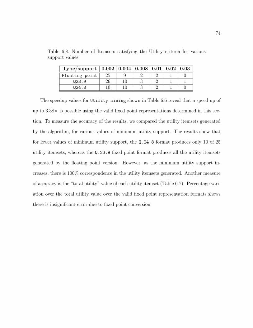
74
Table 6.8. Number of Itemsets satisfying the Utility criteria for varioussupport values
Type/support 0.002 0.004 0.008 0.01 0.02 0.03
Floating point 25 9 2 2 1 0Q23.9 26 10 3 2 1 1Q24.8 10 10 3 2 1 0
The speedup values for Utility mining shown in Table 6.6 reveal that a speed up of
up to 3.38× is possible using the valid fixed point representations determined in this sec-
tion. To measure the accuracy of the results, we compared the utility itemsets generated
by the algorithm, for various values of minimum utility support. The results show that
for lower values of minimum utility support, the Q.24.8 format produces only 10 of 25
utility itemsets, whereas the Q.23.9 fixed point format produces all the utility itemsets
generated by the floating point version. However, as the minimum utility support in-
creases, there is 100% correspondence in the utility itemsets generated. Another measure
of accuracy is the “total utility” value of each utility itemset (Table 6.7). Percentage vari-
ation over the total utility value over the valid fixed point representation formats shows
there is insignificant error due to fixed point conversion.

75
CHAPTER 7
Data Mining Models to Predict Performance of Computer
System Design Alternatives
Computer manufacturers spend a huge amount of time, resources, and money in de-
signing new systems and newer configurations, and their ability to reduce costs, charge
competitive prices, and gain market share depends on how good these systems perform.
Even for a simple system, the process of determining the optimal hardware, i.e., design
space exploration, is a tedious, complex, and time-consuming task. In this work, we
concentrate on both the system design (for regular and parallel computers) and the archi-
tectural design processes and develop methods to expedite them. Our methodology relies
on extracting the performance levels of a small fraction of the machines in the design
space and using this information to develop linear regression and neural network models
to predict the performance of any machine in the whole design space.
7.1. Motivation
Computer manufacturers spend considerable amount of time, resources, and money to
design new desktop/server/laptop systems each year to gain advantage in a market that is
worth hundreds of billions of dollars. When a new computer system is designed, there are
many different types of components (such as CPU type, CPU frequency, motherboard,
memory type, memory size, memory speed, busses, hard disk, etc.) that need to be
configured. It is also hard to understand the different tradeoffs and interactions among

76
these components. Designers cannot also use simulation or other modeling techniques,
because at this high level, the existing models tend to have high inaccuracies resulting in
possibly reducing the efficiency of end systems. As a result, systems designers need to
rely on the existing systems’ performance and their intuitions during the design of new
systems. In this work, we aim to fill this important gap and provide tools to guide the
systems design process.
The design of any computer component is complicated. For example, during the
design of microprocessors, several parts of the processor need to be configured (e.g., cache
size and configuration, number of ALUs, etc. need to be selected). Currently, the most
common methodology architects use is to simulate possible configurations using cycle-
accurate simulators and make decisions based on these outcomes of these simulations.
During the design of a CPU, there are various parameters that need to be set. For
example, in Section 7.4.1 we have selected 24 different parameters that can be varied for
a CPU. If a designer wants to simulate 4 different values for each parameter, then there
are 424 combinations, i.e., the design space consists of 424 elements. Finding the best
configuration that meets the designers’ constraints among these is called the design space
exploration. Each element in the design space can take hours to days to simulate, therefore
it is not possible to simulate all the configurations on a cycle-accurate simulator. This
limits the number of configurations architects can consider. Currently, most designers rely
on heuristics to guide them during this design process, i.e., they rely on heuristics to select
the configurations that are likely to provide the best configuration. For example, simulated
annealing [77] has been used to find the set of configurations they will evaluate. There
are also several methods and heuristics to guide the architectural design space exploration

77
process [55, 25, 66]. Our work is similar to [55, 66] in the sense that we are trying to
create an accurate statistical model for the design space using only a small random subset
of the design space, hence decrease the number of simulations that needs to be completed.
However, our work differs from such approaches in two important ways. First, we use the
same modeling techniques on the systems data published on the SPEC webpage [103]
to create accurate models. In other words, we use the modeling techniques for not only
guiding simulations, but also for predicting performance of real systems. Our claim is
that systems designers can use these predictive models and available data from current
systems, and use them to predict the performance of future systems. The modeling
techniques are especially useful in this area, because there are no reliable simulators to
guide the system designers. Hence, a reduction in the design space can save significant
amount of research/development cost for the companies. Second, even for the simulation
data, we show that our models provide higher accuracy levels than the existing methods.
7.2. Overview of Predictive Modeling
In this section, we develop two types of models. These models correspond to how
the designers can utilize the predictive models. Both approaches are depicted in Figure
7.1. The first one (Figure 7.1(a)) is called sampled design space exploration. It chooses
a random subset of the configurations and using the performance of these configurations
predicts the performance of the rest of the design space. This can be achieved by devel-
oping the selected configurations and evaluating their performance or by simulating the
system on a simulator and using the performance numbers obtained from the simulator for
the selected configurations. Then this data is used to generate a predictive model. As we

78
will describe in Section 7.3, we have developed several models based on linear regression
and neural networks. Using the error estimation provided by modeling and validation
process, we select the model (neural network or linear regression) that provides the high-
est accuracy. This model is then used during the design space exploration to estimate the
performance of the target systems. In addition to this mode of operation, we can also
generate models by using the results of the previous systems in the market. This mode
of operation is called chronological predictive models, which uses historical performance
announcements to predict the performance of future systems. In this modeling task, the
selection of the input data set is determined by the already published results. Let’s as-
sume without loss of any generality that we are trying to estimate the performance of the
systems that will be built in 2007. We can then utilize the results announced in 2006 to
develop a model. In other words, we can use the 2006 results as our training data. We
estimate the error of the developed models using the 2006 data set and then use the best
model to predict the performances of future systems as shown in Figure 7.1(b). We must
note that there may be other means of utilizing the predictive models during the design
space exploration. However, we restrict ourselves to sampled design space exploration
and chronological predictions, because they exhibit the most beneficial use for the design
space exploration.
An important aspect of our work is the use of real data. In this work, we
do not only show that our models can be effectively used to model simulation data, but
more importantly we show that the real system performance can be accurately predicted.
Specifically, we show that our models have high accuracy on performance numbers created
via simulation and then show that these methods also achieve high accuracy when data

79
(a) (b)
Figure 7.1. Overview of design space exploration using predictive modeling:(a) sampled design space exploration and (b) chronological predictive mod-els.
from real systems are used. We train and evaluate our models using previously announced
SPEC results [103]. For example, to develop our models for the chronological estimations,
we utilize the SPEC announcements made in 2005 to train our models and then predict
the performance of the systems announced in 2006. Hence, we can precisely report how
accurately we can estimate the real system performance. We must highlight that SPEC
rating is the most common means of comparing the performance of different systems
and hence they are of tremendous importance to system manufacturers. SPEC ratings
are commonly used for marketing and also used for setting the prices of the systems.
Consequently, system manufacturers put great effort in optimizing their systems for these
ratings.
As we elaborate further in Section 7.4, the complexity and dimensionality of the data
is high: the records based on the simulations include 24 dimensions (i.e., parameters);

80
for SPEC announcements, each record provides information on 32 parameters (repre-
senting the dimensionality of the data) in the system. Each SPEC announcement also
provides the execution times of SPEC applications as well as the SPEC ratings (output
measures). Similarly, the simulations also provide the execution time in terms of cycles
(output measure). Despite the diversity of the data sets, our predictive models are very
accurate in estimating the system performance for both sampled design space exploration
and chronological estimations. Specifically, for sampled design space exploration on sim-
ulation, we obtain 3.5% error rate on average when only 1% of the design space is used
for training. On the other hand, for real system performance prediction, sampled design
space exploration achieves 4.7% error rate on average when only 5% of the data is used.
For chronological predictions, the estimation error is 2.2% on average. Considering the
tremendous cost advantages of using predictive models and such highly accurate predic-
tions, the use of machine learning tools during system design space exploration, therefore,
could be significant competitive advantage.
7.3. Predictive Models
In this work, we use predictive modeling techniques from machine learning [91, 104] to
obtain estimates of performance of systems by using information about their components
as the input. We use a total of ten models. The four linear regression models are described
in the next section and the following Section 7.3.2 discusses the six neural network based
models developed in this work.

81
7.3.1. Linear Regression (LR) Models
Regression analysis is a statistical technique for investigating and modeling the relation-
ship between variables. In this model, we have n observations y=y1,. . . ,yn called the
response variables and xi=xi,1,. . . ,xi,p for i=1..n that are predictor or regressor variables.
The simplest linear regression is of the form y=β0+β1x+ε. In this formula β represents
the coefficients used in describing the response as a linear function of predictors plus a
random error ε. In our input data set we have multiple predictor variables, causing the
response y to be related to p regressor/predictor variables. The model then becomes
y= β0+β1x+β2x+. . . +βpx+ε, where y and x are vectors of n numbers (observations).
This model is called multiple linear regression, which describes a hyperplane in the p-
dimensional space of the regressor variables xi. The fitting of a regression model to the
observations is done by solving the p+1 β coefficients. The method of least squares error
(LSE) is used to estimate the regression coefficients. In this model, it is assumed that
the error term ε has E(ε)=0, Var(ε)=σ2, and that the errors are uncorrelated. Hence the
least-square equation is of the form [78]
S(β0, β1, . . . , βp) =n∑
i=1
ε2i =
n∑i=1
(yi − β0 −p∑
j=1
βjxij)2(7.1)
S(β) may be minimized by solving a system of p+1 partial derivatives of S with respect to
βij ∈ [0,p]. The solutions to these equations are the estimates for the coefficients β. We
used the linear regression model inside the SPSS Clementine [101] tool. In Clementine
there are 4 available methods for creating the linear regression models. The Enter (LR-
E) method puts all predictor variables into the equation using LSE for model creation.

82
In this method, no predictor selection is performed in building the model. The second
method is Stepwise (LR-S) in which the equation is built in steps. The initial model is
the simplest model possible without any input predictors in the equation. At each step,
input predictors that have not been added to the model are evaluated. If the best of these
input predictors improves the predictive power significantly, it is added to the model. In
addition, input predictors that are currently in the model are re-evaluated to determine
if any of them can be removed. This process is repeated until no other fields are added
or removed. The Backwards (LR-B) method of field selection is similar to the LR-S in
that the model is built in steps. However, in this model, the initial model contains all of
the input fields as predictors, and fields can only removed from the model. Input fields
that contribute little to the model are removed form the model until no more fields can
be removed without significantly degrading the model. The Forwards (LR-F) method is
essentially the opposite of LR-B method. The initial model is the simplest model with no
input predictors, and the predictors can only be added to the model. In our experiments,
for sampled design space we have seen that the Backwards (LR-B) method produced the
best results. Therefore, we only present results for LR-B. Generally, we found that the
linear regression models can be built quickly for our system. It took on the order of
milliseconds to generate the models from our input data set.
7.3.2. Neural Network (NN) Models
Neural networks, or more accurately, Artificial Neural Networks (ANN), have been mo-
tivated by the recognition that the human brain processes information in a way that is

83
fundamentally different from the typical digital computer [91]. A neural network, some-
times called multilayer perceptron, is basically a simplified model of the way the human
brain processes information. It works by simulating a large number of interconnected sim-
ple processing units that resemble abstract versions of neurons. The multilayer perceptron
(feedforward ANN) are multivariate statistical models used to relate p predictor variables
x1,. . . ,xp to q response variables y1,. . . ,yq. The model has several layers, each consisting
of either the original or some constructed variables. The most common structure contains
three layers: the inputs which are the original predictors, the hidden layer comprised of
a set of constructed variables, and the output layer made up of the responses. Figure 7.2
depicts an ANN with multiple hidden layers.
Figure 7.3 depicts a hidden unit where the activation function can be linear, hard limit,
sigmoid, or tan-sigmoid function. The model is very flexible containing many parameters
and it is this feature that gives a neural network a nearly universal approximation property.
The usual approach to estimate the parameters is to estimate them by minimizing the
overall residual sum of squares taken over all responses and all observations. This is a
nonlinear least-squares problem. Often backpropagation procedure, which is a variation
of steepest descent, is used.
We used the SPSS Clementine tool to create the ANN models. The neural network
node provides five different training methods, and we have introduced a sixth one. The
first method is Quick (NN-Q), which uses rules of thumb and characteristics of the data
to choose an appropriate shape (topology) for the network. The method usually produces
smaller hidden layers than other methods. As a result, the models are faster to train and
generalize better. Single layer (NN-S) method is a modified version of NN-Q and has a

84
Figure 7.2. Multiple Layered ANN Figure 7.3. An example of ahidden unit
constant learning rate. This model is similar to that of generated by Ipek et al. [55].
This method uses only one hidden layer, which is smaller than the other methods. The
Dynamic (NN-D) method creates an initial topology but modifies the topology by adding
and/or removing hidden units as training progresses. The third method, Multiple (NN-
M), creates several networks of different topologies (the exact number depends on the
training data). These networks are then trained in a pseudo-parallel fashion. At the end of
training, the model with the lowest RMS (Root Mean Square) error is presented as the final
model. Prune (NN-P) method starts with a large network and prunes the weakest units in
the hidden and input layers as training proceeds. This method is comparably slower, but
yields better results than the previously mentioned models. Lastly, the software provides
exhaustive prune (NN-E) method, which is related to the NN-P method. In this model,
network training parameters are chosen to ensure a very thorough search of the space of
possible models to find the best one. This method is the slowest of all, but it often yields

85
the best results. During our analysis of the models, we have observed that the time it
takes to build the neural network models vary significantly. While some of the models
take on the order of seconds to build, the NN-E models can take up to an hour for the
largest input data sets. However, relative to the time and cost of building a real system,
these development times are still negligible.
Another distinction between the different neural network models is their training
methodologies, which are described in Appendix A.
7.3.3. Error Estimation using cross-validation
Clementine software does not provide the estimated predictive error for the model it
creates. In model creation, Clementine randomly divides the training data into two equal
sets, using half of the data to train the model and the other half to simulate. To get
an accurate estimate for the estimated predictive error, we have used 2 different sets of
5-fold cross-validation. We have generated five random sets of 50% of the training data.
In the first set of cross-validation, 4 of the groups are used to create the predictive models
using different methods. Then, the developed model is tested on the left out data group
to calculate the estimated error. Afterwards, the group selection is rotated, i.e., groups 1
through 4 is used for model creation and group 5 for estimated error calculation; groups 2
through 5 is used for model creation and group 1 for estimated error calculation; etc.. The
second set of cross-validation that we have used employs 3 sets to create the model, and
2 sets of data to calculate the estimated error. We similarly perform group rotation to
extract the 5-fold cross-validation. We have observed that these 2 different cross-validation
schemes produce similar results, and in general the second one produces estimations that

86
are closer to the true error rates. However, since the former cross-validation uses more
records during training, its true error rates can be lower. We have taken the average
predictive error on these data sets, as well as the maximum of the error. Both of the error
estimates are very close, and in general maximum gives a closer estimate. Therefore, in
the following sections we will only present the estimates using the maximum error. Note
that the true error rates of the models are calculated by using the created models on the
whole (100% of the) data.
7.3.4. Data Preparation and Input Parameters
Data preparation is an important part of the predictive modeling. In our experiments,
Clementine software automatically scales the input data to the range 0-1 to prevent the
effect of scales of different parameters. The linear regression methods expect the input
parameters to be numerical. Therefore some of the inputs to Clementine (as they will be
presented in the following section) need to be mapped to numeric values. For example,
the input parameter SMT can take the values of yes/no, which can easily be converted
to values 0 and 1. For some other input parameters this kind of transformation is not
possible, hence these are omitted by Clementine. However, neural network models can
have any type of input (numeric, flag, categorical), and are automatically transformed
and scaled to be used in model generation.
In this work, we feed all the input available parameters to Clementine. Then the pro-
gram automatically measures the importance of the parameters, and depending on the
methodology adds or removes predictor variables to the model. In some of the chronolog-
ical design space experiments Clementine omits some predictor variables because these

87
input parameters does not have any variation (e.g. single L2 cache size configuration).
Other than this kind of predictor variable elimination, we don’t discard any input.
7.4. Prediction Results
In our analysis we have used the SPEC benchmark. There are several possible meth-
ods of presenting SPEC performance numbers. This work contains two interrelated parts.
The first one is the use of real systems information that has been gathered. This data has
been used for both sampled design space exploration and chronological predictive model-
ing. The second part is architectural design space exploration of a processor. The data
has been generated using a cycle accurate microarchitecture simulator, and only sampled
design space exploration scheme has been applied. For the first setup, we have used the
published SPEC numbers. The most common SPEC number, SPECint2000 rate (and
SPECfp2000 rate), is the geometric mean of twelve (fourteen) normalized ratios. Specif-
ically, SPEC CPU 2000 contains 12 integer applications, 14 floating-point applications,
and base runtimes for each of these applications. A manufacturer runs a timed test on
the system, and the time of the test system is compared to the reference time, by which
a ratio is computed. The geometric mean of these ratios provides the SPEC ratings.
These ratings are important for companies because it is the means how companies com-
pare their products with others in the market, and form their marketing strategies. The
SPECint2000 rate is the geometric mean of the ratios for the 12 integer applications. In
this work, we are interested in being able to estimate this rate, because it is the most
important metric used for determining the system performance, price, and marketability.
Hence, in the following sections we present the accuracy of our techniques for this rate.

88
For the second setup, we have used the number of cycles the simulated processor consumes
to run the SPEC applications
In the next section, we present the simulation framework that we have used and
provide the details of the data that we used in the real system framework. After that, we
present predictions for sampled design space for real systems in Section 7.4.2. Then, in the
following Section 7.4.3, we present the predictive models for chronological estimations, i.e.,
the results when the training data set contains records from year 2005 and the predicted
data set contains records from year 2006, for single processor and multiprocessor systems,
respectively. Last, in Section 7.4.4 sampled design space of a processor is presented when
data from the simulations are used.
7.4.1. Framework
For modeling of real system performance we use both of the prediction schemes: Sam-
pled Design Space, and Chronological Estimations. For these models, we use the SPEC
announcements. SPEC contains results announced since 1999. Hence, we have to first
prune the data before developing our models. Specifically, the SPEC results contain an-
nouncements from Intel , Alpha, SGI, AMD, IBM, Sun Ultra SPARC, etc. based systems.
Among these, we have chosen to analyze the systems based on AMD Opteron (Opteron),
Intel Pentium D (Pentium D), Intel Pentium 4 (Pentium 4), and Intel Xeon (Xeon). We
also model multiprocessor systems based on AMD Opteron: 2, 4, and 8 way Shared Mem-
ory Multiprocessors (SMPs), corresponding to AMD Opteron 2, 4, and 8, respectively.
The main reason for this selection is that these systems are the most commonly used
systems, which is also evidenced by the low number of SPEC entries with the remaining

89
Table 7.1. Data statistics obtained from SPEC announcements
StatisticsAMD AMD AMD AMD Intel Intel Intel
Opteron Opteron 2 Opteron 4 Opteron 8 Pentium D Pentium 4 XeonRange
2.21 2.47 1.70 1.68 1.45 7.70 1.34(Max/Min)Variation
0.15 0.15 0.12 0.13 0.10 0.37 0.09(Stdev/Mean)
Number of210 197 158 58 144 241 216
records
processors. We analyze the systems based on the processor type because we have observed
that when different processor types are used, the system configurations were significantly
different from each other, preventing us from making a relative comparison.
In Table 7.1, we provide information regarding basic data statistics for all the stud-
ied processor families. Here, we can see that the performance numbers have significant
variation. An important property of the announcements is that even within a single
processor family, the performance numbers showed significant variation: Opteron based
systems has 210 records with a range of 2.21× (i.e., the best system has 2.21× better
performance than the worst system) and variation of 0.15; Opteron 2 based systems have
197/2.47/0.15, Opteron 4 based systems have 158/1.70/0.12, Opteron 8 based systems
have 58/1.68/0.13, Pentium D based systems have 144/1.45/0.10, Pentium 4 based sys-
tems have 241/7.70/0.37 and Xeon based systems have 216/1.34/0.09 records/range/vari-
ation values. For the Chronological Modeling, a subset of this data has been used
and the different performance numbers are as follows: Opteron based systems have
138/1.40/0.08, Opteron 2 based systems have 152/1.58/0.11, Pentium D based systems
have 66/3.72/0.34. The SPEC announcements contain information about the systems as

90
Table 7.2. Data set obtained from SPEC announcements (32 dimensions/columns)
Record Filename Gzip Vpr . . . Processor Bus freq. . . . Hard drive . . .
1 1763.2 2208.2 Intel Xeon 1333 250. . . . . . . . . . . . . . . . . . . . . . . . . . . . . . . . . . . . . . . . . . . . . . . . . . .3550 361.8 292.9 Pentium 3 133 n/a
well as execution times of each application. Each announcement provides the configura-
tion of 32 system parameters: company, system name, processor model, bus frequency,
processor speed, floating point unit, total cores (total chips, cores per chip), SMT (yes/no),
Parallel (yes/no), L1 instruction and data cache size (per core/chip), L2 and L2 data cache
size (on/off chip, shared/nonshared, unified/nonunified), L3 cache size (on/off chip, per
core/chip, shared/nonshared, unified/nonunified), L4 cache size (# shared, on/off chip),
memory size and frequency, hard drive size, speed and type, and extra components. Cur-
rently, there are 7032 announced results (3550 integer and 3482 floating-point). Based on
these parameters and the complete set, we first generated the data set described in Table
7.2. This data set is used throughout the development and of evaluations of our models
in this section.
In addition to predicting the real system performance (Sampled Design Space and
Chronological Estimations), we also perform modeling of simulation of processor outcome
(Sampled Design Space). For the processor sampled design space models, we use Sim-
pleScalar [70] tool set, which is a system software infrastructure used to build modeling
applications for program performance analysis, detailed microarchitectural modeling, and
hardware-software co-verification. We do not use any particular feature of the simulator
in our models; hence our approach may be applied to other simulator frameworks. For
our analysis, based on the work by Phansalkar et al. [89] we have selected 12 applications

91
from the SPEC2000 benchmark. The results for the following applications are presented:
Applu (fp), Equake (fp), Gcc (int), Mesa (fp), and Mcf (int). The remaining results are
similar. In our simulation framework, we use a partial simulation technique to reduce
time for simulation per each application, while incurring a slight loss of accuracy, because
the SPEC applications runs billions of instructions, and simulators are usually slow. Since
we want to get simulations for all the configurations in our design space, it is impossible
to run the applications to completion. We have used SimPoint [98], which uses Basic
Block Distribution Analysis as an automated approach for finding the small portions of
the program to simulate that are representative of the entire program’s execution. This
approach is based upon using profiles of a program’s code structure (basic blocks) to
uniquely identify different phases of execution in the program. We use the simulation
points given by SimPoint and execute 100 Million instructions for each interval.
Table 7.3 shows the parameters used for the microprocessor study, which corresponds
to 4608 different configurations per benchmark. Note that this corresponds to performing
4608 simulations for each target benchmark. Table 7.4 gives the range of the simulated
execution cycles (i.e., the ratio of the fastest to slowest configuration for each benchmark)
and the variance of them. We can see that the range of the results can be very wide for
some applications (e.g., mcf has a range of 6.38×). Despite this range, our models can
predict the simulation outcome very accurately by using a small fraction of the simulation
data.

92
Table 7.3. Configurations used in microprocessor study
Parameters Values
L1 Data Cache Size 16, 32, 64 KBL1 Data Cache Line Size 32, 64 B
L1 Data Cache Associativity 4L1 Instruction Cache Size 16, 32, 64 KB
L1 Instruction Cache Line Size 32, 64 KBL1 Instruction Cache Assoc. 4
L2 Cache Size 256, 1024 KBL2 Cache Line Size 128 B
L2 Cache Associativity 4, 8L3 Cache Size 0, 8 MB
L3 Cache Line Size 0, 256 BL3 Cache Associativity 0, 8
Branch PredictorPerfect, Bimodal, 2-level,
CombinationDecode/Issue/Commit Width 4, 8
Issue wrong Yes, NoRegister Update unit 128, 256
Load/Store queue 64, 128Instruction TLB size 256, 1024 KB
Data TLB size 512, 2048 KBFunctional Units (ialu, imult, memport, fpalu, fpmult) 4/2/2/4/2, 8/4/4/8/4
Table 7.4. Data statistics obtained from SPEC benchmark simulations
Statistics Applu Equake Gcc Mesa McfRange (Max/Min) 1.62 1.73 5.27 2.22 6.38
Variation (Stdev/Mean) 0.16 0.19 0.33 0.19 0.71
7.4.2. Sampled Design Space Modeling of a Computer System
In this section we present results investigating the accuracy of our models. In these
models, we randomly sampled 2% to 10% of the data to build our models, and then
used the entire data set to predict the accuracy of our models. As described in Section
7.2, this approach can be used to reduce the design space size and hence accelerate the

93
Figure 7.4. Estimated vs. true error rates for Opteron based systems
design space exploration. The percentage error is calculated by the formula: 100*|yi-
yi|/yi, where yi is the predicted and yi is the true (reported) number for the ith record in
the data used. By using only the training set during cross-validation (c.f. Section 7.3.3),
we also extract estimated error rates for each model. Figures 7.4 through 7.8 present
the estimated error and the true error rates (when the model is applied to the complete
design space) for the five different platforms. In each figure, we present the accuracy of
the linear regression (leftmost chart), the neural network with exhaustive prune (middle),
and the neural network with single layer (rightmost). In each of these charts, we present
the accuracy of the corresponding model when the sampling rate is set to 2%, 3%, 4%,
5%, and 10% of the whole data set.
Figure 7.4 presents the results for the estimated and true error rates for the LR-B,
NN-E and NN-S methods on Opteron systems for varying the sampling rate. For the
linear regression, we observe that the difference between the estimated error and the true
error rates is generally small. We also observe that the estimated error is higher than

94
Figure 7.5. Estimated vs. true error rates for Opteron 2 based systems
the true error rates when less than 5% of the design space is used for estimation. The
estimated error rates are close to the true error for 5% and 10% samples. In the neural
network methods, we see that the exhaustive method has a slightly higher error rate than
the single layer method. The backwards method of linear regression produces the best
results, and has a prediction accuracy of 95.68% accuracy at 4% sampling.
The results for the Opteron 2 system are shown in Figure 7.5. Similar to the Opteron
based systems, we can conclude that the estimation error is generally small and pessimistic
(i.e., higher than the true rates) for small sampling rates, and becomes very accurate with
increasing data set size.
An important property of all the presented results is that as the training set size is
increased, the accuracy of the models generally increases. This is expected because with
a larger training set, the variations in the design space can be modeled better. However,
when we consider the results presented in Figure 7.5, we see that at 4% sampled design
space the estimated and true error rates for all the methods increase compared to 3%

95
Figure 7.6. Estimated vs. true error rates for Pentium 4 based systems
sampling. This is indication that the extra points added to the 3% design space to
create the 4% sample design space makes the method over-fit to the training data (hence
increasing the error rate on different data). Therefore, it is possible that a larger sample
rate will produce a model that results in higher error rates.
Figure 7.6 presents the results for the Pentium 4 based systems. In these results, the
error rates for the prediction accuracy are higher than the previously discussed systems
unless a high sampling rate is used. One reason for this inaccuracy is that the range of
Pentium 4 machines is very wide (the fastest machine is more than 7× faster than the
slowest machine). Hence, the systems are very different from each other and the selected
training points are not always representative of the whole design space. However, when a
larger data set is used for model creation, the accuracy increases rapidly.
Pentium D based system results are presented in Figure 7.7. The results for all model-
ing techniques are close; linear regression model is slightly better than the neural network
models. Also, the prediction results are very accurate for this processor family. The

96
Figure 7.7. Estimated vs. true error rates for Pentium D based systems
Figure 7.8. Estimated vs. true error rates for Xeon based systems
reason for this is that the data points are very similar to each other, because Pentium D
results contain less than 2 years of data. Therefore, there have not been major changes
in the systems based on Pentium D processors. The estimated error rates are also close
to the true error rates. When compared to other systems, we see that neural networks
are optimistic when estimating the error rates. A similar observation can be made for the

97
Xeon systems (presented in Figure 7.8). Such a behavior is generally observed when the
prediction accuracy is very good. The prediction accuracy is generally better when there
is little variation among the different systems. As a result, the training set used during
the development of the model tends to contain similar records and particularly the neural
network models are able to fit to these elements tightly. This results in very low estimated
error rates (note that the estimated error rates are found using only the training data set).
On the other hand, we must note that the inaccuracy of the estimated error rates is not
likely to make a difference, because all the models provide high accuracy for such cases.
In Section 7.4.5, we provide a summary of the results, where we also present the accuracy
of a scheme, which will choose its model based on the estimated errors and show that
such a scheme is highly accurate.
Figure 7.8 presents the Xeon based system results. For the Xeon systems, we have the
best prediction accuracy between all the processor families: the linear regression model
achieves 96.7% accuracy at 3% sampling rate.
7.4.3. Chronological Predictive Modeling
In the previous section, we have shown that the predictive models achieve high prediction
accuracies for estimating the performance of systems from a small subset of manufactured
systems configurations. This section presents the results for chronological predictive mod-
els for single processor and multiprocessor based systems, which use historical performance
announcements to predict the performance of future systems. We used the published re-
sults in 2005 to predict the performance of the systems that were built and reported in
2006.

98
In Figure 7.9, we present the prediction error for different Linear Regression and Neural
Network models for Intel Xeon, Intel Pentium 4, and Intel Pentium D based systems. The
percentage error is calculated by 100*|yi-yi|/yi, where yi is the predicted and yi is the true
(reported) number for the ith record in the data used. The mean and standard deviation
of the percentage prediction error are shown by circles and error bars, respectively. In
general, we see that Linear Regression models perform better than Neural Networks. One
of the main reasons for this is the fact that neural networks tend to over-fit to the data.
In our case, the model built using 2005 data is very accurate for predicting 2005 data,
however when we try to predict 2006, the over-fitting causes larger errors in estimations.
However, linear regression does not have this problem and is successful in predicting 2006
results. In Figure 7.9, we see the best accuracy is achieved using with linear regression
enter (LR-E) method of linear regression with an error rate of 2.1%, 1.5%, and 2.2% for
Intel Xeon, Intel Pentium 4, and Intel Pentium D based systems, respectively. Figure
7.10(a) shows the results for Opteron based systems. The accuracies of the models are
similar to the other single processor families. For Pentium D (Figure 7.9c), all the models
perform about the same and produce roughly 2% error rate. The reason for this is that
the data points are very similar to each other, because Pentium D results contain less
than 2 years of data. Therefore, there have not been major changes in the systems based
on Pentium D processors and as a result, the neural network models are as successful as
the linear regression models.
In Figure 7.10, we present the 1, 2, 4, 8 processor results for AMD Opteron based
systems. The prediction accuracy results for the multiprocessor systems are similar to
the single processor cases. A trend that we observe is that going to more complex systems,

99
(a) (b) (c)
Figure 7.9. Chronological predictions for Xeon (a), Pentium 4 (b), PentiumD (c) based systems
(a) (b)
(c) (d)
Figure 7.10. Chronological predictions for Opteron based multiprocessorsystems: (a) one processor, (b) two processors, (c) four processors, and (d)eight processors

100
Opteron-2 (Figure 7.10(b)) to Opteron-4 (Figure 7.10(c)) to Opteron-8 (Figure 7.10(d)),
we have a slightly higher minimum error rate of 3.1%, 3.2%, and 3.5%, respectively.
These minimum error rates are achieved with the stepwise (LR-S) and backward (LR-B)
methods. Here we see that LR-S/LR-B methods perform significantly better than the
LR-E method. The reason for this is LR-E method uses all predictors as input and hence
the model has a tighter fit to the training data, while LR-S method only adds a predictor
to the model if it improves the quality of the model significantly. Likewise, LR-B method
removes predictors if the predictor does not improve the quality of the model above a
specified threshold. Hence, LR-S and LR-B methods converge to the same model in these
cases. In these examples we see that LR-S/LR-B methods use lesser predictors than LR-
E and perform better on the test (future) data. Another observation is that the neural
networks perform poorer than linear regression models. Their prediction rate seems to
get highly inaccurate as the number of processors in the system increases.
7.4.4. Sampled Design Space Modeling of a Processor
In this section, we present the prediction accuracy results for the sampled design space
exploration of a microprocessor. For these experiments, prediction models are created by
randomly sampling 1% to 5% of the data and then using this data subset to build (train)
the models. We then extract estimated error rates for each model using the approach
presented in previous section and the true error rates are calculated using the entire data
set. As described in Section 7.2, this approach can be used to reduce the design space
size and hence accelerate the design space exploration. In Figures 7.11 through 7.15, we
present the mean of the percentage prediction error, which is calculated by 100*|yi-yi|/yi,

101
where yi is the predicted and yi is the true (reported) number for the ith record in the
data used. In general, we observe that neural network models have better prediction rates
than linear regression models. This relative success is expected because neural networks
are better at modeling complex data sets.
In this section we present the results for the best Linear Regression model (LR-B)
and the best Neural Network model (NN-E), and a fast Neural Network model (NN-
S). The general trend shows that as the training sample size increases from 1% to 5%,
we obtain better prediction accuracy. This is due to the fact that the smaller training
sets include less/insufficient information to capture the underlying complex relationship
between design parameters. In some instances, we may observe that the error rates may
have increased a little or stayed about the same when going to a higher training sample
size. The main reason for this is the random selection of the training set. Even though
the data selection is random, it is possible that the selected points may not be uniform
through out the design space; hence the created model fits a portion of the space very
accurately and not fitting the rest. Another point to observe is that Neural Network
models generally have better prediction accuracy than Linear Regression models. This
is due to the fact that linear models are inadequate to model the nonlinear changes and
predictor interactions, while neural networks’ complex data modeling capabilities provide
a good fit of the results and hence highly accurate predictions. As it is seen in Figure 7.11,
for the Applu application NN-E achieves 1.8% error rate when 1% of the design spaced is
used in training. This rate drops below 1% error as the training data set size is increased
to 2%. For NN-E, we observe a similar behavior for Equake (Figure 7.12) and Mcf (Figure
7.14) applications. On the other hand, Gcc (Figure 7.13) and Mesa (Figure 7.15) exhibit
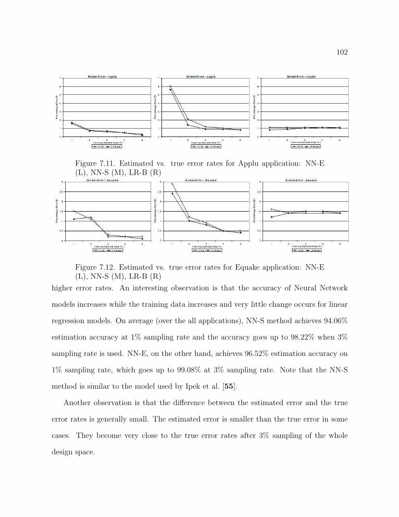
102
Figure 7.11. Estimated vs. true error rates for Applu application: NN-E(L), NN-S (M), LR-B (R)
Figure 7.12. Estimated vs. true error rates for Equake application: NN-E(L), NN-S (M), LR-B (R)
higher error rates. An interesting observation is that the accuracy of Neural Network
models increases while the training data increases and very little change occurs for linear
regression models. On average (over the all applications), NN-S method achieves 94.06%
estimation accuracy at 1% sampling rate and the accuracy goes up to 98.22% when 3%
sampling rate is used. NN-E, on the other hand, achieves 96.52% estimation accuracy on
1% sampling rate, which goes up to 99.08% at 3% sampling rate. Note that the NN-S
method is similar to the model used by Ipek et al. [55].
Another observation is that the difference between the estimated error and the true
error rates is generally small. The estimated error is smaller than the true error in some
cases. They become very close to the true error rates after 3% sampling of the whole
design space.

103
Figure 7.13. Estimated vs. true error rates for Gcc application: NN-E (L),NN-S (M), LR-B (R)
Figure 7.14. Estimated vs. true error rates for Mcf application: NN-E (L),NN-S (M), LR-B (R)
Figure 7.15. Estimated vs. true error rates for Mesa application: NN-E(L), NN-S (M), LR-B (R)
7.4.5. Summary
In the previous sections, we have presented the results for SPEC published results for real
systems and SPEC benchmark simulation results for the microprocessors. The summary

104
Table 7.5. Average accuracy results from SPEC published results
Statistics 2% 3% 4% 5% 10%LR-B 9.1 8.3 5.5 4.6 3.5NN-E 11.1 9.8 8.9 7.8 5.6NN-S 10.8 9.5 8.8 8.1 6.0Select 9.3 7.9 5.8 4.7 3.8
of the results presented in Section 7.4.2 are summarized in Table 7.5. The last row, select
method, shows the error rates that would be achieved if the method that gives the best
result on the estimation is used for predicting the whole data set. The models developed
in this section include 5 to 7 predictor variables. Within these, there are usually two or
three factors that are significantly more important than others. The important factors
and their order of importance change from a processor family to another. For example,
for the Pentium 4 systems, the most important parameters for neural networks (with their
relative importance presented in parenthesis) are processor speed (0.503) L2 cache size
(0.501), memory size (0.279), bus frequency (0.145), and L1 instruction cache size (0.115).
Note that the importance factor denotes the relative importance of the input factor (0
denoting that the field has no effect on the prediction and 1.0 completely determines the
prediction). For the same predictions LR model has processor speed, memory size and
L2 cache size with standardized beta coefficients of 0.510, 0.406 and 0.123, respectively.
Standardized beta coefficients show the relative importance of the predictor variable.
Table 7.6 summarizes the results presented in the previous section 7.4.3. In this
table, we present the best accuracy achieved and the method that achieves it for different
systems. As mentioned previously, linear regression models perform well, achieving error
rates ranging between 1.5% and 3.5% on single and multiprocessor systems. We have also
done a similar analysis to the generated models as in the sampled design space exploration.

105
Table 7.6. The best accuracy achieved for single processor and multipro-cessor chronological design space exploration and the model that achievesthis accuracy
Prediction XeonPentium Pentium
OpteronOpteron Opteron Opteron
D 4 2 4 8Accuracy 2.1 2.2 1.5 2.1 3.1 3.2 3.5
Method LR-E LR-E LR-ELR-B/ LR-B/ LR-B/ LR-B/LR-S LR-S LR-S LR-S
The models described in Section 7.4.3 include 3 to 10 predictor variables. Within these,
there are generally two or three factors that are significantly more important than others.
The important factors and their order of importance change from a processor family
to another. For example, for the Opteron systems, (Figure 7.10) the most important
parameters for neural networks (with their relative importance presented in parenthesis)
are processor speed (0.659), memory frequency (0.154), L2 being on chip or off chip
(0.147), and L1 data cache size (0.139). For the same predictions, the linear regression
model included processor speed and memory size with standardized beta coefficients of
0.915 and 0.119, respectively. While for Pentium D based systems (Figure 7.9c), the
important factors used in the neural network model are processor speed (0.570), L2 cache
size (0.500), L1 cache being shared or not (0.206), L2 cache being shared or not (0.154),
L1 data cache size (0.145), and bus frequency (0.120). Linear regression, on the other
hand, uses processor speed (0.733), L2 cache size (0.583), memory size (0.001), memory
frequency (0.094), and L1 cache size (0.297). Overall, the combinations of all parameters
aid in the high prediction rates we observe.
For the sampled design space exploration using simulation results (Section 7.4.4), we
see that generally neural network methods perform better than linear regression methods.
When we compare the neural network models in themselves, exhaustive prune method

106
Table 7.7. Average accuracy results from SPEC simulations
Statistics 1% 2% 3% 4% 5%LR-B 4.2 4 3.82 3.8 3.8NN-E 3.48 2.04 1.14 0.94 0.88NN-S 5.94 3.18 2.22 1.16 1.5Select 3.4 2.6 1.14 0.94 0.88
has the best prediction accuracy. The summary of the results presented in Section 7.4.4
are summarized in Table 7.7. The results reveal that the select method successfully finds
the best model and uses it for the predictions. Note that for the 1% sampling rate, the
select method performs better than the NN-E.
The reason for this is that for the Applu application, the select method uses the LR-
B, which gives a better accuracy than the NN-E. Therefore, the average accuracy of the
select method is better than the NN-E method.
An important difference between the real system analysis and the simulation analysis
is that the number of available data points is usually small for real system analysis. Hence
the diversity for many of the components is hard to capture in the created models, hence
higher error rates are seen. In simulation data, the huge number of points is created by
keeping the input parameters as constant and changing only one parameter at a time.
Even with sampling 1% of the data, the diversity can be captured, and it is easier for the
predictive models to achieve higher accuracy on simulation data.

107
CHAPTER 8
Profit-Aware Cache Architectures
Previous works in computer architecture have mostly neglected revenue and/or profit,
key factors driving any design decision. In this section, we evaluate architectural tech-
niques to optimize for revenue/profit. In this work we have utilized our pricing models
created by data mining methods to estimate the increase in revenue when new microarchi-
tectural techniques are applied to caches. First, we present some motivational background
for our work followed by our pricing models.
8.1. Speed-binning
The research literature is filled with architectural optimizations that seek to improve
various design goals such as performance, power consumption, reliability, and security.
However, the evaluation of these concepts tends to neglect one of the key factors driving
any chip manufacturing decision: a company’s bottom-line of revenue or profit. This
shortcoming is understandable, as the relationship between any design metric and profit
is hard to understand. For example, an optimization that improves performance by 10%
will increase profit if a) this increase is valuable/desirable to the consumers, b) the cost of
re-engineering can be amortized over the lifespan of the chip, and c) consequent changes
in other design factors do not decrease the value to the consumers. Therefore, it may
not be possible to estimate the impact of an architectural optimization on revenue pre-
cisely. However, in this paper we will show that we can make accurate estimations on

108
(a) (b)
Figure 8.1. (a) Frequency binning in modern microprocessors. (b) Price vs.frequency of Intel Pentium 4 family
relative impact of different architectural configurations on revenue, and argue that these
estimations should be considered during the design of the processor architectures.
There are two important aspects of profitability: cost and revenue. To increase profit,
one could reduce the cost. For example, chip yield is one obvious scope for optimization in
nanoscale processors [87], as the continuing downward scaling of transistor feature sizes
has made fabrication considerably more difficult and expensive [76, 80, 108]. However,
to get a better understanding of the impact of an architectural scheme, one needs to
understand the effects on revenue as well. For example, an approach that optimizes solely
for yield would not take into account the fact that CPUs concurrently manufactured using
a single process are routinely sold at different speed ratings and prices. This practice
of speed-binning (Figure 8.1(a)) is usually performed by testing each manufactured chip
separately over a range of frequency levels until it fails. As a result of the inherent process
variations, different processors fall into separate speed bins, where they are rated and
marketed differently. Speed-binning thus helps the chip manufacturer create a complete
product line from a single design. Figure 8.1(b) shows an example price distribution

109
representing the Intel Pentium 4 processor family [51]. Assuming a simplified supply and
demand model, the total chip revenue would be the sum of the segmented areas under the
yield curve. Consequently, one way of increasing revenue would be to shift the binning
distribution in such a way that more processors are able to fall into higher-priced bins.
As the importance of process variations increases, controlling the distribution becomes
harder.
8.2. Substitute Cache Scheme
In this work, we propose a cache architecture that aims to improve overall revenue
and profit with post-fabrication modifications. Particularly, in this scheme, the level 1
(L1) cache is augmented with a small Substitute Cache (SC) storing the most critical
cache words whose latencies may have been affected by process variations. Particularly,
in this scheme each way of the L1 cache is augmented with a fully associative data array,
which stores the most critical lines as a result of process variations. In our study, its size
is either 4 or 8 entries. Once the SC holds high-delay words, they are never accessed from
the main array, allowing the L1 cache to run at higher frequencies. In addition to shifting
more chips towards high-priced bins, this scheme also reduces yield losses due to delay
violations. We concentrate on caches because they have been shown to be the critical
component under process variations [49]. Also our analysis reveals that the critical path
lies on the cache in 58.9% of the chips we model. One of the main reasons for this is
that caches consume a relatively large percentage of chip area. Although our technique
will affect various design stages, such changes remain minimal. Therefore, the proposed
technique will have minimal impact on cost. Variable production costs will remain low,

110
as the testing phase can be incorporated into current binning processes. On the other
hand, the proposed scheme will have a significant impact on the binning distribution and
profit as we describe in Section 8.4.
8.2.1. Speed Binning
In order to effectively estimate the binning distribution and demonstrate the effect the
process variation has on it, we chose a set of 1000 chips for our analysis. Most processor
families are available in discrete frequency intervals. For example, the frequency for the
Intel Pentium 4 processor family starts with 3.0 GHz and reaches 3.8 GHz with equal
intervals of 0.2 GHz [51]. Moreover, most commercial processors are marketed with 5 or
6 different frequency ratings. Similarly, our binning methodology assumes equal binning
intervals. This interval is chosen depending on the number of bins to be generated.
8.3. Price Modeling
One of the most important steps in our analysis is to calculate the revenue from a set
of chips once the number of chips in a given bin distribution is known. To achieve this,
we have to know the price of the chips for any given bin. Then, once the price of a chip in
a particular bin is known, we can calculate the total revenue by multiplying the number
of chips in that bin with the corresponding price level.
Our goal in this section is to develop a model that can predict the price of a chip
given its architectural configuration (including its frequency). However, we must note
that we do not need absolute prices. Particularly, we are interested in the change in the
revenue for a bin distribution change rather than estimating the gross revenue. Thus, a

111
model that provides the relative prices of chips is sufficient to understand the impact of
architectural configurations on revenue.
To develop our models, we used historical pricing information of different Intel proces-
sor families [51]. Specifically, we first generate our input data, which includes a record for
each of the 114 available processors. These records include information about the L1 data
and instruction cache size, L2 cache size, L2 cache being shared or not, L3 cache size,
processor frequency, front side bus frequency, release date, process generation, address
space, socket type, wattage, number of cores, and threads per core. Then, a subset of
this input data is used to train regression and neural network models. The remaining
elements are used to estimate the accuracy of the models (i.e., validation). Then, based
on this estimation, we choose a specific model to predict the prices of a new architecture.
In our analysis we used regression analysis and neural networks similar to the one
described in Section 7.3. During our analysis we have grouped the list of processors into
three different categories: desktop, mobile, and server. We mainly focus on and present
results for the desktop processors; the remaining processor types provide similar results.
Rather than using the raw input data directly, we divide our database into ten groups.
We randomly leave one group out (test data), and then use the rest of the nine groups for
model creation and validation, i.e., groups 1 through 8 is used for model creation and group
9 (validation data) is used to estimate the error of the created model; groups 2 through 9
is used for model creation and group 1 (validation data) used for error estimation and so
on. Using these nine models, we approximate the error rate by finding the error during
the prediction of the test and validation groups. The model with the lowest error is used
for estimating the prices. For our input set, the minimum error rate is achieved with

112
the NN-Q method, which provides 1.9% average error rate for the processors in the test
data. NN-Q includes 11 out of the 14 predictor variables. The important factors used in
the neural network model (with their relative importance presented in parenthesis) are
front side bus frequency (0.34), clock frequency (0.30), number of cores (0.22), threads
per core (0.14), L2 cache size (0.09) and the release date (0.07), where 0 denotes that the
field has no effect on prediction and 1.0 denoting that the field completely determines the
prediction. We have to note that these importance factors does not need to add up to
1, i.e., the sum can be greater than 1. In our analysis, we generally observe that neural
networks outperform the regression methods. One of the reasons is that the price curves
are usually sublinear in lower frequency bins and there are rapid increases as we move
to higher processor frequencies. The neural network models capture these non-linearities
effectively. The working of the models can be seen at our price prediction website [88].
These results show that using the subset of the processors available, we can create a
very accurate model presenting the relation between the processor properties and its price,
in other words, they show that there is a significant correlation between the price of the
processor and its configuration, even though markets are also influenced by the preferences
of the consumers interacting in it. The existence of such a relation is not surprising,
though, as prices of chips are largely determined by their value to the consumers. This
value, in turn, depends highly on the performance of the chip, which is strongly tied to
its configuration/properties (e.g., performance of a processor can be accurately predicted
from its configuration as we have shown in previous Chapter 7 and other works [55, 66]).
This forms a link between the configuration of a processor and its price/value. Our

113
models can unveil this relation and accurately estimate the price of a processor from its
architectural configuration. We use these models to calculate the revenue results.
8.4. Revenue Estimation and Profit
This section describes the analysis of the total revenue and the implications on the
profit. It is important to note that, in all the following studies a simplistic market sup-
ply/demand model is assumed where all fabricated chips can be sold at predicted/predeter-
mined price levels according to their clock frequencies. Since a real-life demand model
would depend on various other factors, the resulting numbers given in this section should
be considered as potential increase in revenue or profit. The binning data obtained in the
previous section is used in revenue calculation. The chips that fall in the higher/faster
bins after testing are sold with higher prices than those lying in the lower/slower bins.
To have an estimate of this increased revenue, we use the model that provides the highest
accuracy among the models studied in Section 8.3. Our architectural configuration is fed
into our price models (described in Section 8.3) to find the relative prices of the chips in
each bin. These relative prices are found to be 1, 1.03, 1.13, 1.39, and 2.84, for the Bin0
through Bin4 for the 5-bin strategy and 1, 1.02, 1.09, 1.23, 1.63, and 4.00, for the Bin0
through Bin5 for the 6-bin strategy. Then, the number of chips in different bins for the
base case (without any resizing) is multiplied with their respective prices to calculate the
revenue for the base case. Using the same methodology, the revenues of SC schemes are
calculated based on their new binning distribution. The relative change in revenue is then
calculated with respect to the revenue of the base case.

114
(a) (b)
Figure 8.2. Binning with (a) 5-bin and (b) 6-bin strategy for SC- 4 and SC-8 schemes
Figure 8.2 (a) and 8.2 (b) show the binning results for the base, SC-4, and SC-8
schemes for 5-bin and 6-bin strategies, respectively. To understand these figures, consider
the leftmost bar for each bin. This bar corresponds to the number of chips in that bin for
the base cache architecture. The bars next to it (i.e., the one in the middle) represent the
number of chips in that bin when SC-4 scheme is applied. The bars on the right represent
the number of chips in the corresponding bin for the SC-8 scheme. In general, we see that
cache redundancy can successfully increase the number of chips in the higher bins. For
example, the number of chips in the highest bin (Bin4) is increased by 23.2% using SC-8.
It is misleading to draw any conclusion about high-frequency chip yield by simply
considering the chips in the highest bin. The gain in the highest bins for all the SC schemes
are accompanied by a reduction in the number of chips in the lower bins. However, we
must note that the total yield is increased using these schemes. Specifically, the total yield
increases by 9.0% using SC-8 schemes (for ϕ=0.5). However, since the SC is associated
with a power overhead there is yield loss due to power dissipation of the extra data arrays.

115
The SC-8 scheme causes an additional 10.3% loss of chips in the category of power-related
losses. In spite of this loss, the total yield increases for SC, because it converts a high
number of delay loss chips into yield. Even though the total number of chips increases,
the schemes tend to move a larger number of chips towards the higher bins. As a result,
the chip counts in the lower bins tend to decrease.
Table 8.1. Increase in revenue for various cache-architectures
Range factor (ϕ) Binning strategyIncrease in revenue with respect to
the base architecture [%]MWS OWS SC4 8 4 8 4 8
0.55-bin 1.94 7.52 1.88 6.05 5.03 12.606-bin 1.54 6.26 1.54 5.13 3.90 11.41
0.35-bin 2.19 7.35 2.19 6.08 6.98 12.006-bin 1.70 6.9 1.70 6.46 5.54 13.14
Table 8.1 presents the increase in revenue obtained using different microarchitectural
schemes. For ϕ=0.5, the SC-8 scheme increases the revenue by up to 12.60% and 13.14%
for the 5-bin and 6-bin strategies, respectively. Note that, the SC scheme has a power
consumption overhead and hence causes some power-related yield losses. However, despite
the increase in the power consumption, we are observing that the SC scheme tends to
provide better revenues because it is able to generate an elevated number of chips in higher
bins. We must note that the increase in revenue is smaller compared to the increase in
the number of chips in the highest bin. Take for example the 6-bin case; for SC-8, a
15.0% increase in the number of chips in the highest (i.e., highest-priced) bin results in
an increase of the total revenue by only 11.4%. The main reason behind this can be
explained as follows. Due to the normal distribution nature of the binning curve, the

116
yield in the next-highest bin is higher. This bin also has a high price gradient and hence
it constitutes a large fraction of the overall revenue. We observe that the number of chips
in this bin either reduces or stays roughly constant. As a result, the increase in total
revenue is limited by a moderate percentage.
Using the same revenue results, we can also estimate profit. Let’s assume that the
cost per chip is identical, which equals to 80% of the selling price of the lowest frequency
chip. This means, the cost of each chip is 0.8 in terms of our relative price. Therefore,
the total cost for 1000 chips (note that even the chips that do not meet delay or leakage
constraints contributes to cost) is 800. We can then subtract this amount from the total
revenues and find the profit. If we apply this methodology, we find that the SC-8 increases
the profit in the 5-bin strategy by 46.6%. For a chip company, which invests billions of
dollars in the manufacturing process, this extra revenue can prove to be a considerable
margin. It should be noted we are neglecting the extra testing costs needed for the new
cache design.

117
CHAPTER 9
Learning and Leveraging the Relationship between
Architecture-Level Measurements and Individual User
Satisfaction
The ultimate goal of computer design is to satisfy the end-user. In particular comput-
ing domains, such as interactive applications, there exists a variation in user expectations
and user satisfaction relative to the performance of existing computer systems. In this
work, we leverage this variation to develop more efficient architectures that are customized
to end-users. We first investigate the relationship between microarchitectural parameters
and user satisfaction. We study a group of users to characterize the relationship between
the hardware performance counters (HPCs) and individual user satisfaction levels. Based
on this analysis, we use artificial neural networks to model the function from HPCs to user
satisfaction for individual users. This model is then used online to predict user satisfaction
and set the frequency level accordingly.
9.1. Motivation
Any architectural optimization (performance, power, reliability, security, etc.) ulti-
mately aims at satisfying the end-user. However, understanding the happiness of the user
during the run of an application is complicated. Although it may be possible to query the
user frequently, such explicit interaction will annoy most users. Therefore, it would be

118
beneficial to estimate user satisfaction using implicit metrics. Traditionally, computer ar-
chitects have used implicit metrics such as instructions retired per second (IPS), processor
frequency, or the instructions per cycle (IPC) as optimization objectives. The assumption
behind these metrics is that they relate in a simple way to the satisfaction of the user.
When two systems are compared, it is assumed, for example, that the system providing
a higher IPS will result in higher user satisfaction. For some application domains, this
assumption is generally correct. For example, the execution time of a long running batch
application is largely determined by the IPS of the processor. Hence, increasing IPS will
result in an increase in user satisfaction. However, in this section we show that the re-
lationship between hardware performance and user satisfaction is complex for interactive
applications and an increase in a metric like IPS does not necessarily result in an increase
in user satisfaction. More importantly, we show that the relationship between hardware
performance and user satisfaction is highly user-dependent. Hence, we explore the feasi-
bility of estimating individual user satisfaction from hardware metrics, develop accurate
nonlinear models to do so, and use these models for run-time power management.
Driving architectural decisions from estimates of user satisfaction has several advan-
tages. First, user satisfaction is highly user-dependent. This observation is not surprising.
For example, an expert gamer will likely demand considerably more computational power
than a novice user. In addition, each user has a certain taste; for example, some users
prefer to prolong battery life, while others prefer higher performance. If we know the
individual users satisfaction with minimal perturbation of program execution, we will be
able to provide a better experience for the user. Second, when a system optimizes for

119
user satisfaction, it will automatically customize for each application. Specifically, a sys-
tem that knows the users satisfaction with a given application will provide the necessary
performance to the user. For interactive applications, this may result in significant advan-
tages such as power savings or increased lifetime reliability. For example, one of our target
applications exhibits no observable change in performance when the frequency of the pro-
cessor is set to its lowest level. In this case, our system drastically reduces the power
consumption compared to traditional approaches without sacrificing user satisfaction.
9.2. Hardware Performance Counters
Modern microprocessors include integrated hardware performance counters (HPC) for
non-intrusive monitoring of a variety of processor and memory system events [6, 28, 29].
HPCs provide low-overhead access to a wealth of detailed performance information related
to CPU’s functional units, caches, main memory, etc. Even though this information is
generally statistical in nature, it does provide a window into certain behaviors that are
otherwise impractical to observe.
We use WinPAPI, the Windows variant of PAPI [23], to access the HPCs present
in the processor. In our study we concentrate on the nine specific performance metrics
listed in Table 9.1. These counters are manually selected as a representative set of the
HPCs available on the Pentium M. The choice of using only nine counters is due to a
WinPAPI limitation. We collect counter values every 100 ms. WinPAPI automatically
time multiplexes and scales the nine event counters.

120
Table 9.1. Hardware counters we use in our experiments
PAPI Counter DescriptionPAPI TOT INS Instructions issuedPAPI RES STL Cycles stalled on any resourcePAPI TOT CYC Total cyclesPAPI L2 TCM Level 2 cache missesPAPI BTAC M Branch target address cache missesPAPI BR MSP Conditional branch instructions mispredictedPAPI HW INT Hardware interruptsPAPI L1 DCA Level 1 data cache accessesPAPI L1 ICA Level 1 instruction cache accesses
9.3. Experimental Setup
To explore the relationships between different microarchitectural parameters and user
satisfaction, we conduct two sets of studies with 20 users. Our experiments are done
using an IBM Thinkpad T43p with a 2.13 GHz Pentium M-770 CPU and 1 GB memory
running Microsoft Windows XP Professional SP2. The laptop is tethered to the power
outlet during all experiments. Although eight different frequency levels can be set on
the Pentium M-770 processor, only six can be used due to limitations in the SpeedStep
technology. For both user studies, we experiment with three types of applications: a 3D
Shockwave animation, a Java game, and high-quality video playback. Since we target
the CPU in this paper, we picked three applications with varying CPU requirements: the
Shockwave animation is very CPU-intensive, the Video places a relatively low load on the
CPU, and the Java game falls between these extremes.
9.4. Relation between user Satisfaction and Hardware Performance Counters
The primary objective of our first user study is to explore the correlation between
HPCs and user satisfaction. The monitored hardware counters are listed in Table 9.1. In

121
this first set of experiments, the users are asked to carry out the three application tasks as
described in the previous sections. During execution, we randomly change the frequency
and ask the users to verbally rank their experience on a scale of 1 (discomfort) to 10
(very comfortable). Users typically provided a satisfaction rating within 5-10 seconds.
These satisfaction levels are then recorded along with the HPC readings and analyzed
as described in the next section. Then we compute the maximum, minimum, average,
range, and the standard deviation of the counter values for up to 5 seconds within the
given interval. The end result is a vector of 45 metrics for each satisfaction level reported
by the user. Note that since we have performed the user studies with 20 users and three
applications, we collected 360 user satisfaction levels.
We then find the correlation of the 45 metrics to the user satisfaction rating by using
the formula:
rx,y =N
∑xy − (
∑x)(
∑y)√
[N∑x2 − (
∑x)2][N
∑y2 − (
∑y)2]
(9.1)
Pearsons Product Moment Correlation Coefficient (r) is commonly used to find cor-
relation among two data series (x and y) and results in a value between -1 and 1. If the
correlation is negative, the series have negative relationship; if it’s positive, the relation-
ship is positive. The closer the coefficient is to either -1 or 1, the stronger the correlation
between the variables. Thus, the magnitude of these correlations allows us to compare
the relative value of each independent variable in the predicting the dependent variable.
The correlation factors for each of the 45 parameters and the user rating are presented
in Appendix B. In summary, we observe a strong correlation between the hardware met-
rics and user satisfaction rating: there are 21 parameters that correlate with the user

122
satisfaction rating by a factor above 0.7 (all these 21 parameters have a factor ranging
between 0.7 and 0.8) and there are 35 parameters with factors exceeding 0.5. On one
hand, this result is intuitive; it is easy to believe that metrics representing processor per-
formance relate to user satisfaction. On the other hand, observing the link between such
a high-level quantity as measured user satisfaction and such low-level metrics as level 2
cache misses is intriguing.
We classify the metrics (and their correlations with user satisfaction) based on their
statistical nature (mean, maximum, minimum, standard deviation, and range). The mean
and standard deviation of the hardware counter values have the highest correlation with
user satisfaction rating. A t-test analysis shows with over 85% confidence that mean and
standard deviation both have higher r values when compared to the minimum, maximum,
and range of the HPC values. We analyze the correlations between the satisfaction results
and user. Note that the r value cannot be used for this purpose, as the user numbers are
not independent. Instead, we repeatedly fit neural networks to the data collected for each
application, attempting to learn the overall mapping from HPCs to user satisfaction. As
the inputs to the neural network, we use the HPC statistics along with a user identification
for each set of statistics. The output is the self-reported user satisfaction rating. In each
fitting, we begin with a three-layer neural network model using 50 neurons in the hidden
layer. After each model is trained, we perform a sensitivity analysis to find the effect of
each input on the output. Sensitivity analysis consists of making changes at each of the
inputs of the neural network and observing the corresponding effect on the output. The
sensitivity to an input parameter is measured on a 0 to 1 scale, called the relative impor-
tance factor, with higher values indicating higher sensitivity. By performing sensitivity

123
analysis, we can find the input parameters that are most important in determining an
output parameter, i.e., user satisfaction. During this process, we consistently find that the
user number input has by far the highest relative importance factor. Averaging across all
of our application tasks, the relative importance factor of the user number is 0.56 (more
than twice as high as the second factor). This strongly demonstrates that the user is the
most important factor in determining the rating.
Finally, to understand the nature of the relationship between the HPCs and the user
satisfaction, we analyze the trends for different functions for user satisfaction as provided
by the user at each of the processor frequencies. We have plotted the user satisfaction
against the different frequencies. Most of the trends can be placed in four major categories:
• Constant - User satisfaction remains unchanged with frequency.
• Linear - User satisfaction increases linearly with processor frequency.
• Step - User satisfaction is the same for a few high frequencies but then plummets
suddenly for the remaining lower ones.
• Staircase - User satisfaction takes on discrete values that monotonically increase
with increasing frequency.
These results reveal several important trends. First, user satisfaction is often non-linearly
related to processor frequency. Second, user satisfaction is application-dependent, and
finally, user satisfaction is user-dependent.
9.5. Predictive User-Aware Power Management
Based on the initial user study results, we developed a power management scheme
that sets the frequency of the processor based on estimates of user satisfaction. This

124
(a) (b)
Figure 9.1. Framework of the predictive user-aware power management
section presents this predictive user-aware power management scheme, called Individu-
alized Dynamic Frequency and Voltage Scaling (iDVFS). To implement iDVFS, we have
built a system that is capable of predicting a user’s satisfaction based on interaction with
the system. The framework can be divided into two main stages as depicted in Figure
9.1: Learning Stage - The proposed system is initially trained based on reported user
satisfaction levels and hardware performance counter values. Artificial neural networks
are trained offline to learn the function from HPC values to user satisfaction. Runtime
Power Management - Before execution, the learned model is loaded by the system. Dur-
ing run time, the HPC values are sampled, entered into the predictive model, and then
the predicted user satisfaction is used to dynamically set the processor frequency.
9.6. Predictive Model Building
The learning stage helps us to gather data that associates an individual user’s satisfac-
tion with different hardware performance counter readings and statistics. These functional

125
instances are used to build a predictive model that estimate the satisfaction of that par-
ticular user from the HPCs. We use neural networks (specifically NN-E explained in
Section 7.3.2) to learn this model. We have also experimented with regression models and
decision trees, but the neural networks provided the highest accuracy.
Our experiments represent a very interesting case for machine learning. Typically,
machine learning algorithms are extensively trained using very large data sets (e.g., thou-
sands of labeled training inputs). We would like to use NNs for their ability to learn
complex non-linear functions, but do not have a very large data set. For each application-
user pair, we only have six training inputs; one for each processor frequency. A training
input consists of a set of HPC statistics and a user-provided satisfaction label. When
we first began building NN models with all 45 inputs (9 HPC counters with 5 statistics
each), we noticed that our models were overly conservative, only predicting satisfaction
ratings within a narrow band of values. We used two training enhancements to permit
the construction of accurate NN models. First, we simplified the NN by limiting the
number of inputs. Large NNs require large amounts of training data to sufficiently learn
the weights between neurons. To simplify the NN, we used the two counters that had the
highest correlation, specifically PAPI BTAC M-avg and PAPI TOT CYC-avg (as shown
in Appendix B). Second, we repeatedly created and trained multiple NNs, each beginning
with different random weights. After 30 seconds of repeated training, we used the most
accurate NN model. These two design decisions were important in allowing us to build
accurate NN models.
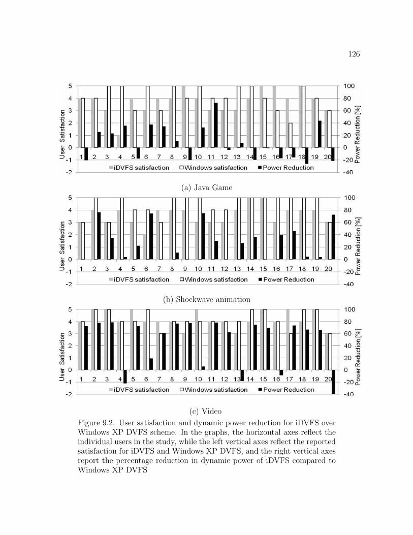
126
(a) Java Game
(b) Shockwave animation
(c) Video
Figure 9.2. User satisfaction and dynamic power reduction for iDVFS overWindows XP DVFS scheme. In the graphs, the horizontal axes reflect theindividual users in the study, while the left vertical axes reflect the reportedsatisfaction for iDVFS and Windows XP DVFS, and the right vertical axesreport the percentage reduction in dynamic power of iDVFS compared toWindows XP DVFS

127
9.7. Experimental Results
In this section, we evaluate the predictive user-aware power management scheme with
a user study. We perform a second set of user studies in which the users are asked to
carry out the same tasks. This time, the durations of the applications are increased: the
Java Game is executed for 2.5 minutes; Shockwave and Video are executed for 1.5 minutes
each. The user is asked to execute the application twice, once for Windows XP DVFS and
once for iDVFS, which loads the individual neural network model for the user/application
before the start of the execution. Once the execution completes, the users are asked to
rate their satisfaction with each of the systems on a scale of 1 (very dissatisfied) to 5 (very
satisfied).
The dynamic power consumption of a processor is directly related to frequency and
supply voltage and can be expressed using the formula P = V 2CF , which states that
power is equal to the product of voltage squared, capacitance, and frequency. By using the
frequency traces and the nominal voltage levels on our target processor [43], we calculated
the relative dynamic power consumption of the processor. Figure 9.2 presents the CPU
dynamic power reduction achieved by the iDVFS algorithm compared to the Windows
XP DVFS algorithm for the individual users for each application. It also presents their
reported satisfaction levels. To understand the figure, consider a group of three bars for
a particular user. The first two bars represent the satisfaction levels for the users for the
iDVFS (gray) and Windows (white) schemes, respectively. The third bar (black) shows
the power saved by iDVFS for that application compared to the Windows XP DVFS
scheme (for which the scale is on the right of the figure). On average, our scheme reduces
the power consumption by 8.0% (Java Game), 27.9% (Shockwave), and 45.4% (Video)

128
compared to the Windows XP DVFS scheme. A one-sample t-test of the iDVFS power
savings shows that for Shockwave and Video, iDVFS decreases dynamic power with over
95% confidence. For the Java game, there are no statistically-significant power savings.
Correspondingly, the average user satisfaction level is reduced by 8.5% (Java Game), 17.%
(Shockwave), and remains the same for Video. A two-sample paired t-test comparing the
user satisfaction ratings from iDVFS and Windows XP DVFS indicates that for Java
and Video, there is no statistical difference in user satisfaction when using iDVFS. For
Shockwave, we reduce user satisfaction with over 95% confidence
The combined results show that for Java, iDVFS is no different than Windows XP
DVFS, for Shockwave, iDVFS trades off a decrease in user satisfaction for a decrease in
power consumption, and for the Video, iDVFS significantly decreases power consumption
while maintaining user satisfaction.
9.7.1. Total System Power and Energy-Satisfaction Trade Off
In the previous section, we have presented experimental results indicating the user sat-
isfaction and the power consumption for three applications. For two applications (Video
and the Java Game), we concluded that the iDVFS users are at least as satisfied as
Windows XP DVFS users. However, for the Shockwave application, we observed that
although the power consumption is reduced, this is achieved at the cost of a statistically
significant reduction in average user satisfaction. Therefore, a designer needs to be able
to evaluate the success of the overall system. To analyze this trade-off, we developed a
new metric called the energy-satisfaction product (ESP) that works in a similar fashion to
popular metrics such as energy-delay product. Specifically, for any system, the ESP per

129
Figure 9.3. Improvement in energy consumption, user satisfaction, andenergy-satisfaction product for the Shockwave application
user/application can be found by multiplying the energy consumption with the reported
satisfaction level of the user.
Clearly, to make a fair comparison using the ESP metric, we have to collect the total
system energy consumption during the run of the application. Once the system energy
measurements are collected (for both Windows XP DVFS and iDVFS), we find the ESP
for each user by multiplying their reported satisfaction levels and the total system energy
consumption. The results of this analysis are presented in Figure 9.3. In this figure, we
present the reduction in system energy consumption, increase in user satisfaction, and
change in ESP for each user. Hence, the higher numbers correspond to improvement
in each metric, whereas negative numbers mean that the Windows XP DVFS scheme
performed better. Although the ESP improvement varies from user to user, we see that
iDVFS improves the ESP product by 2.7%, averaged over all users. As a result, we can
conclude that Windows XP DVFS and iDVFS provide comparable ESP levels for this

130
particular application. In other words, the reduction in user satisfaction is offset at a
significant benefit in terms of power savings.

131
CHAPTER 10
Conclusion
As the data sizes available to common users as well as businesses increase akin to
Moores Law of data, existing solutions to extracting information from them slowly be-
come obsolete. Data mining has already emerged as an attractive alternative in a number
of domains including business (marketing, credit scoring, and decision systems), science
(climate modeling, astrophysics, and biotechnology), security (intrusion detection, fraud
detection) and others such as search engines and video analysis. As they are more widely
used, it is clear that the existing approach to computing becomes inadequate necessitat-
ing application-specific architectures to optimize their performance. A new data mining
benchmark is required for workload characterization and architecture evaluation. In this
work, we presented Minebench, a diverse benchmark suite of data mining applications,
to enable development of superior algorithms and systems for data mining applications.
Using MineBench, we establish the fact that data mining applications form a unique
workload distinguishing them from conventional applications. We have studied important
characteristics of the applications when executed on an 8-way SMP machine. Overall, our
results indicate that there is ample scope for improvement in the performance of both
data mining algorithms and systems.
In our study, we found that if the core kernels of data mining applications are smartly
extracted, high performance setups can be realized. In our work, we proposed a generic

132
data mining system architecture using reconfigurable logic. Further, we design and im-
plement hardware accelerators for two sample applications. The results indicate that our
designs achieve significant speedups over software-only implementations, in addition to
meeting area and bandwidth constraints. The success of these designs make a strong case
for further research on hardware accelerators for data mining applications.
In another part of our work, we have described a method for implementation of data
mining algorithms on embedded systems. Data mining algorithms are designed and im-
plemented for conventional computing systems, and show poor performance while exe-
cuting on an embedded system. We applied our methodology to several representative
data mining applications and have shown that significant speedups can be achieved. We
also quantized the error in each case and determined the optimum configurations for
fixed point implementation. Particularly, with our fixed point conversion methodology
we achieve significant speedups, as much as 11.5×, with minimal loss of accuracy. As
embedded data mining assumes importance in various key fields, our methodology will
serve as a starting step towards efficient implementations.
The second area of focus in this work is the applications of the data mining to archi-
tectural problems. We have looked at multiple problems. In the design space exploration
work, we have used two different machine learning techniques, linear regression and neural
network. The design space exploration is an important task for all system manufacturers.
The possible combinations of system parameters that can be set is generally huge and
the models we generate in this work can be used to estimate the performance of various
systems by using a small fraction of the design space as a training set. Also these re-
sults indicate that the designers can estimate the performance of new systems using the

133
limited data available for the already built systems and use them to estimate similar as
well as future systems. The system manufacturers can use current system configuration
and important factors provided by the models to start the search towards a system that
will provide the highest performance. As a result, these models will reduce design and
development cost.
The other important points from the application of data mining to architecture is
that: a) we can create a very accurate model presenting the relation between the proces-
sor properties and its price, in other words, there is a significant correlation between the
price of the processor and its configuration, even though markets are also influenced by
the preferences of the consumers interacting in it b) we have demonstrated that there is
a strong, albeit usually nonlinear, link between low-level microarchitectural performance
metrics, as measured by hardware performance counters and user satisfaction for interac-
tive applications. More importantly, we show that the link is highly user-dependent.
10.1. Future Work
Increasing power densities and diminishing returns from deeper pipelines have elimi-
nated increasing clock frequency as means of achieving higher performance. As a result,
the design space of future high-performance processors has shifted to chip multiproces-
sors (CMPs) [86, 46, 50]. Currently there has not been any thorough analysis of data
mining workloads on these emerging technologies. There has been recent studies by Li
et al. [110] from Intel on understanding the memory performance of some data mining
applications on different sized CMPs. We believe that an analysis similar to the one we
have presented in Chapter 4 will be of great use to the architecture community. Also as we

134
have mentioned in Section 5.3 GPUs are becoming an important hardware to accelerate
computation and it would be interesting to measure the performance and scalability of
more complex data mining applications running on GPUs.
Another area that we should look into is the design space exploration, analysis and
modeling of applications on CMP systems using simulators. There are several publicly
available full system simulators supporting chip multi-processors, such as PTLSim [7],
Simics [72] and M5 Simulator [17]. Currently we are looking into the effects of different
compiler optimizations for parallel applications. We have seen that having the highest
optimization level is not always the best performing code. We also want to explore
how core assignment/partitioning affects applications performance when multiple multi-
threaded workloads are running in parallel and be able to create a model to predict an
applications performance with as little simulations as possible.

135
References
[1] R. Agrawal, A. Arning, T. Bollinger, M. Mehta, J. Shafer, and R. Srikant. TheQuest data mining system. In Proceedings of the 2nd International Conference onKnowledge Discovery in Databases and Data Mining, August 1996.
[2] R. Agrawal, H. Mannila, R. Srikant, H. Toivonen, and A.I. Verkamo. Fast discoveryof association rules. Advances in Knowledge Discovery and Data Mining, pages 307–328, 1996.
[3] K. Albayraktaroglu, A. Jaleel, X. Wu, M. Franklin, B. Jacob, C. Tseng, and D. Ye-ung. BioBench: A benchmark suite of bioinformatics applications. In Proceedings ofThe 5th International Symposium on Performance Analysis of Systems and Software(ISPASS), March 2005.
[4] D. H. Albonesi. Selective cache ways: on-demand cache resource allocation. In Pro-ceedings of the ACM/IEEE International Symposium on Microarchitecture (MI-CRO), October 1999.
[5] C. Ambroise and G. J. McLachlan. Selection bias in gene extraction on the basis ofmicroarray gene-expression data. Proceedings of the National Academy of Sciences,99(10):6562–6566, 2002.
[6] AMD. BIOS and Kernel Developer’s Guide for AMD Athlon64 and AMD OpteronProcessors, 2006.
[7] Matt T. Yourst (Computer Architecture and Power-Aware Systems (CAPS) re-search group at the State University of New York at Binghamton). Ptlsimx86-64 cycle accurate processor simulation design infrastructure. Available athttp://www.ptlsim.org, 2006.
[8] D. Bader, Y. Li, T. Li, and V. Sachdeva. BioPerf: A benchmark suite to evaluatehigh-performance computer architecture on bioinformatics applications. In Proceed-ings of the IEEE International Symposium on Workload Characterization (IISWC),October 2005.

136
[9] D. A. Bader, V. Sachdeva, V. Agarwal, G. Goel, and A. N. Singh. BioSPLASH:A sample workload for bioinformatics and computational biology for optimizingnext-generation performance computer systems. Technical report, University of NewMexico, May 2005.
[10] Z. Baker and V. Prasanna. An architecture for efficient hardware data mining usingreconfigurable computing system. In Fourteenth Annual IEEE Symposium on FieldProgrammable Custom Computing Machines 2006 (FCCM ’06), April 2006.
[11] Z. Baker and Viktor Prasanna. Efficient hardware data mining with the Apriorialgorithm on FPGAs. In Proceedings of the Thirteenth Annual IEEE Symposium onField Programmable Custom Computing Machines (FCCM ’05), 2005.
[12] Z. K. Baker and V. P. Prasanna. Efficient parallel data mining with the Apriorialgorithm on FPGAs. In Proceedings of 13th Annual IEEE Symposium on Field-Programmable Custom Computing Machines (FCCM), April 2005.
[13] S. Barrachina, M. Castillo, F. D. Igual, R. Mayo, and E. S. Quintana-Orti. Evalua-tion and tuning of the level 3 cublas for graphics processors. In IEEE InternationalSymposium on Parallel and Distributed Processing (IPDPS), April 2008.
[14] S. Barrachina, M. Castillo, F. D. Igual, R. Mayo, and E. S. Quintana-Orti. Solvingdense linear systems on graphics processors. In Proceedings of the 14th internationalEuro-Par conference on Parallel Processing, August 2008.
[15] A. Bateman, L. Coin, R. Durbin, R.D. Finn, V. Hollich, S. Griffiths-Jones,A. Khanna, M. Marshall, S. Moxon, E. L. L. Sonnhammer, D. J. Studholme,C. Yeats, and S. R. Eddy. The Pfam protein families database. Nucleic Acids Re-search, 32(Database):D138–D141, 2004.
[16] J. C. Bezdek. Pattern Recognition with Fuzzy Objective Function Algorithms. KluwerAcademic Publishers, 1981.
[17] N. L. Binkert, R. G. Dreslinski, L. R. Hsu, K. T. Lim, A. G. Saidi, and S. K.Reinhardt. The m5 simulator: Modeling networked systems. IEEE Micro, 2006.
[18] OpenMP Architecture Review Board.
[19] S. Borkar, P. Dubey, K. Kahn, D. Kuck, H. Mulder, S. Pawlowski, and J. Rattner.Platform 2015: Intel processor and platform evolution for the next decade. IntelCorporation, 2005. White Paper.

137
[20] J. Bradford and J. Fortes. Performance and memory-access characterization of datamining applications. In Workload Characterization: Methodology and Case Studies,pages 49–59, November 1998.
[21] B. Brock and K. Rajamani. Dynamic power management for embedded systems. InIn Proceedings of IEEE International Systems-on-Chip, September 2003.
[22] A. J. Brookes, H. Lehvaslaiho, M. Siegfried, J. G. Boehm, Y. P. Yuan, C. M. Sarkar,P. Bork, and F. Ortigao. HGBASE: a database of SNPs and other variations in andaround human genes. Nucleic Acids Research, 28(1):356–360, January 2000.
[23] S. Browne, J. Dongarra, N. Garner, G. Ho, and P. Mucci. A portable programminginterface for performance evaluation on modern processors. International Journalof High Performance Computing Applications, 14(3):189–204, 2000.
[24] Y. Cai and Y. X. Hu. Sensory steam data mining on chip. In Second NASA DataMining Workshop: Issues and Applications in Earth Science, May 2006.
[25] J. Cavazos, C. Dubach, and G. Fursin. Automatic performance model constructionfor the fast software exploration of new hardware designs. In International Con-ference on Compilers, Architecture and Synthesis for Embedded Systems (CASES),August 2006.
[26] Y. Chen, Q. Diao, C. Dulong, W. Hu, C. Lai, E. Li, W. Li, T. Wang, and Y. Zhang.Performance scalability of data-mining workloads in bioinformatics. Intel TechnologyJournal, 09(12):131–142, May 2005.
[27] K. Choi, R. Soma, and M. Pedram. Dynamic voltage and frequency scaling basedon workload decomposition. In Proceedings of the International Symposium on LowPower Electronics and Design (ISLPED), August 2004.
[28] Intel Corporation. Intel Itanium 2 Processor Reference Manual: For Software De-velopment and Optimization, 2004.
[29] Intel Corporation. Intel 64 and IA-32 Architectures Software Developer’s ManualVolume 3A: System Programming Guide, 2007.
[30] P. Domingos and M. Pazzani. Beyond independence: Conditions for optimality ofthe simple bayesian classifier. In Proceedings of the International Conference onMachine Learning, 1996.

138
[31] C. Dubach, T. M. Jones, and M. F. P. O’Boyle. Microarchitectural design spaceexploration using an architecture-centric approach. In International Symposium onMicroarchitecture (MICRO), December 2007.
[32] L. Eeckhout, S. Nussbaum, J. Smith, and K. De Bosschere. Statistical simulation:Adding efficiency to the computer designer’s toolbox. In International Symposiumon Microarchitecture (MICRO), December 2003.
[33] L. Eeckhout, H. Vandierendonck, and K. D. Bosschere. Quantifying the impact of in-put data sets on program behavior and its applications. The Journal of Instruction-Level Parallelism, 5:1–33, February 2003.
[34] D. J. Eisenstein and P. Hut. Hop: A new group finding algorithm for N-bodysimulations. Journal of Astrophysics, (498):137–142, 1998.
[35] M. Estlick, M. Leeser, J. Szymanski, and J. Theiler. Algorithmic transformations inthe implementation of k-means clusteringon reconfigurable hardware. In Proceedingsof the Ninth Annual IEEE Symposium on Field Programmable Custom ComputingMachines(FCCM 01), 2001.
[36] M. Estlick, M. Leeser, J. Theiler, and J. J. Szymanski. Algorithmic transformationsin the implementation of k-means clustering on reconfigurable hardware. In Proceed-ings of the ACM/SIGDA ninth international symposium on Field programmable gatearrays, February 2001.
[37] S. Eyerman, L. Eeckhout, and K. D. Bosschere. The shape of the processor designspace and its implications for early stage explorations. In 7th WSEAS InternationalConference on Automatic Control, Modeling and Simulation.
[38] Z. Fan, F. Qiu, A. Kaufman, and S. Yoakum-Stover. Gpu cluster for high perfor-mance computing. In ACM/IEEE conference on Supercomputing (SC), November2004.
[39] Y. Fei, L. Zhong, and N. K. Jha. An energy-aware framework for coordinated dy-namic software management in mobile computers. In Proceedings of the Interna-tional Symposium on Modeling, Analysis, and Simulation of Computer and Telecom-munications Systems (MASCOTS), October 2004.
[40] D. Ferrer, R. Gonzalez, R. Fleitas, J. P. Acle, and R. Canetti. NeuroFPGA imple-menting artificial neural networks on programmable logic devices. In Design, Au-tomation and Test in Europe Conference and Exhibition Designers Forum (DATE),February 2004.

139
[41] Gary-Chicago-Milwaukee Corridor Transportation System. GCM Travel.http://www.gcmtravel.com.
[42] A. Ghosh and T. Givargis. Analytical design space exploration of caches for embed-ded systems. In Design, Automation and Test in Europe Conference and Exhibition(DATE), March 2003.
[43] S. Gochman and R. Ronen. The intel pentium m processor: Microarchitecture andperformance. Intel Technology Journal, 2003.
[44] S. Gochman and R. Ronen. The intel pentum m processor: Microarchitecture andperfromance, 2003.
[45] N. K. Govindaraju, B. Lloyd, W. Wang, M. Lin, and D. Manocha. Fast computationof database operations using graphics processors. In Proceedings of the SIGMODInternational Conference on Management of Data, June 2004.
[46] L. Hammond, B. A. Nayfeh, and K. Olukotun. A single-chip multiprocessor. IEEEComputer, September 1997.
[47] J. Han and M. Kamber. Data Mining: Concepts and Techniques. Morgan KaufmannPublishers, August 2000.
[48] R. Hankins, T. Diep, M. Annavaram, B. Hirano, H. Eric, H. Nueckel, and J. Shen.Scaling and characterizing database workloads: Bridging the gap between researchand practice. In Proceedings of the 36th International Symposium on Microarchitec-ture (MICRO), pages 76–87, December 2003.
[49] E. Humenay, D. Tarjan, and K. Skadron. Impact of parameter variations on multi-core chips. In Workshop on Architectural Support for Gigascale Integration.
[50] Intel. Platform 2015: Intel processor and platform evolution for the next decade.ftp://download.intel.com/technology/computing/archinnow/platform2015/download/Platform 2015.pdf, 2005.
[51] Intel. Intel processor pricing. http://www.intel.com/intel/finance/prcelist/procesorprice list.pdf?iid=InvRel+pricelist pdf, 2006.
[52] Intel Corporation. Architecting the era of tera - technical white paper. Available athttp://www.intel.com, 2005.
[53] Intel Corporation. Intel VTune performance analyzer 7.2. Available athttp://www.intel.com, 2005.

140
[54] E. Ipek, B. R. de Supinski, M. Schulz, and S. A. McKee. An approach to performanceprediction for parallel applications. In Euro-Par.
[55] E. Ipek, S. A. McKee, B.R. deSupinski, M. Schultz, and R. Caruana. Efficiently ex-ploring architectural design spaces via predictive modeling. In Architectural Supportfor Programming Languages and Operating Systems (ASPLOS), October 2006.
[56] V. Iyenagar, L. Trevillyan, and P. Bose. Representative traces for processor modelswith infinite cache. In Proceedings of the 2rd International Symposium on High-Performance Computer Architecture (HPCA), pages 62–73, February 1995.
[57] Jung J. H. Cholesky decomposition and linear programming on a gpu. Scholarlypaper, University of Maryland, 2006.
[58] A. Jaleel, M. Mattina, and B. Jacob. Last Level Cache (LLC) performance of datamining workloads on a CMP – a case study of parallel bioinformatics workloads. InProceedings of the 12th International Symposium on High Performance ComputerArchitecture (HPCA), February 2006.
[59] M.V. Joshi, G. Karypis, and V. Kumar. ScalParC: A new scalable and efficientparallel classification algorithm for mining large datasets. In Proceedings of the 11thInternational Parallel Processing Symposium (IPPS), 1998.
[60] N. P. Jouppi. Improving direct-mapped cache performance by the addition of a smallfully-associative cache and prefetch buffers. In In Proceedings of the InternationalSymposium on Computer Architecture (ISCA), May 1990.
[61] T. Karkhanis and J. Smith. A 1st-order superscalar processor model. In Proceedingsof the 31st International Symposium on Computer Architecture (ISCA), June 2004.
[62] K. Keeton, D. Patterson, Y. Q. He, R. Raphael, and W. Baker. Performance char-acterization of a quad Pentium Pro SMP using OLTP workloads. In Proceedings ofthe 25th International Symposium on Computer Architecture (ISCA), pages 15–26,June 1998.
[63] S. Khan, P. Xekalakis, J. Cavazos, and M. Cintra. Using predictive modeling forcross-program design space exploration in multicore systems. In International Con-ference on Parallel Architectures and Compilaton Techniques (PACT), September2007.
[64] J. Kim, X. Qin, and Y. Hsu. Memory characterization of a parallel data miningworkload. In Workload Characterization: Methodology and Case Studies, pages 60–70, November 1998.
141
[65] P. Krishnamurthy, J. Buhler, R. Chamberlain, K. Gyang M. Franklin, and J. Lan-caster. Biosequence similarity search on the mercury system. In 15th IEEE Inter-national Conference on Application-Specific Systems, Architectures and Processors(ASAP), September 2004.
[66] B. C. Lee and D. M. Brooks. Accurate and efficient regression modeling for mi-croarchitectural performance and power prediction. In Architectural Support forProgramming Languages and Operating Systems (ASPLOS).
[67] C. Lee, Miodrag Potkonjak, and William H. Mangione-Smith. MediaBench: A toolfor evaluating and synthesizing multimedia and communications systems. In Pro-ceedings of 30th Annual International Symposium on Microarchitecture (MICRO),pages 330–335, December 1997.
[68] Y. Li, T. Li, T. Kahveci, and J. Fortes. Workload characterization of bioinfor-matics applications. In Proceedings of the 13th IEEE International Symposium onModeling, Analysis, and Simulation of Computer and Telecommunication Systems(MASCOTS), pages 15–22, September 2005.
[69] Y. Liu, W. K. Liao, and A. Choudhary. A two-phase algorithm for fast discovery ofhigh utility itemsets. In Proceedings of the Pacific-Asia Conference on KnowledgeDiscovery and Data Mining (PAKDD), May 2005.
[70] SimpleScalar LLC. Simplescalar tool set. http://www.simplescalar.com.
[71] J. MacQueen. Some methods for classification and analysis of multivariate obser-vations. In Proceedings of the Berkeley Symposium on Mathematical Statistics andProbability, 1967.
[72] P. S. Magnusson, M. Christensson, J. Eskilson, D. Forsgren, G. Haallberg, J. Hog-berg, F. Larsson, A. Moestedt, and B. Werner. Simics: A full system simulationplatform. Computer, 2002.
[73] A. Mallik, J. Cosgrove, R. P. Dick, G. Memik, and P. Dinda. Picsel: measuringuser-perceived performance to control dynamic frequency scaling. In InternationalConference on Architectural Support for Programming Languages and OperatingSystems (ASPLOS), October 2008.
[74] A. Mallik, B. Lin, G. Memik, P. Dinda, and R. P. Dick. User-driven frequencyscaling. IEEE Computer Architecture Letters, 5(2):16, 2006.
142
[75] D. Menard, D. Chillet, F. Charot, and O. Sentieys. Automatic floating-point tofixed-point conversion for DSP code generation. In Proceedings of International Con-ference on Compilers, Architecture and Synthesis for Embedded Systems (CASES),October 2002.
[76] Mark Miller. Manufacturing-aware design helps boost ic yield.http://www.eetimes.com/news/design/features/showArticle.jhtml;?articleID=47102054,September 2004.
[77] F. Moja, M. J. Moja, and J. C. Lopez. Evaluation of design space explorationstrategies. In EUROMICRO Conference, 1999 September.
[78] D. C. Mongomery, E. A. Peck, and G. C. Vining. Introduction to Linear RegressionAnalysis. Wiley, April 2001.
[79] R. Narayanan, D. Honbo, J. Zambreno, G. Memik, and A. Choudhary. An fpgaimplementation of decision tree classification. In Design, Automation and Test inEurope Conference(DATE), March 2007.
[80] S.R. Nassif. Modeling and analysis of manufacturing variations. In IEEE CustomIntegrated Circuits.
[81] M. L. Norman, J. Shalf, S. Levy, and G. Daues. Diving deep: Data managementand visualization strategies for adaptive mesh refinement simulations. Computingin Science and Engineering, 1(4):36–47, 1999.
[82] A. Nukada, Y. Ogata, T. Endo, and S. Matsuoka. Bandwidth intensive 3-d fft kernelfor gpus using cuda. In Proceedings of the ACM/IEEE conference on Supercomputing(SC), November 2008.
[83] NVIDIA. CUDA Programming Guide. http://developer.download.nvidia.com/compute/cuda/2 0/docs/NVIDIA CUDA Programming Guide 2.0.pdf.
[84] NVIDIA. CUDA Software Development Kit. http://developer.download.nvidia.com/compute/cuda/sdk/website/samples.html.
[85] NVIDIA. GeForce 8800 GPU Architecture Overview.http://www.nvidia.com/object/IO 37100.html.
[86] K. Olukotun, B. A. Nayfeh, L. Hammond, K. Wilson, and K. Chang. The casefor a single-chip multiprocessor. In Proceedings of the 7th International Confer-ence on Architectural Support for Programming Languages and Operating Systems(ASPLOS-VII), October 1996.
143
[87] S. Ozdemir, D. Sinha, G. Memik, J. Adams, and H. Zhou. Yield-aware cache archi-tectures. In International Symposium on Microarchitecture (MICRO).
[88] Berkin Ozisikyilmaz, Abhishek Das, Gokhan Memik, andAlok Choudhary. Processor pricing prediction models.http://www.ece.northwestern.edu/boz283/Processor Price Prediction.html, 2008.
[89] A. Phansalkar, A. Joshi, L. Eeckhout, and L. John. Measuring program similarity:Experiments with spec cpu benchmark suites. In IEEE International Symposiumon Performance Analysis of Systems and Software, March 2005.
[90] Jayaprakash Pisharath. Design and Optimization of Architectures for Data IntensiveComputing. PhD thesis, Northwestern University, 2005.
[91] R. Ramakrishnan and J. Gehrke. Database Management Systems. McGraw-Hill,August 2000.
[92] P. Ranganathan, K. Gharachorloo, S. Adve, and L. Barroso. Performance of data-base workloads on shared-memory systems with out-of-order processors. In Proceed-ings of the 8th International Conference on Architectural Support for ProgrammingLanguages and Operating Systems (ASPLOS-VIII), pages 307–318, October 1998.
[93] S. Roy and P. Banerjee. An algorithm for trading off quantization error with hard-ware resources for MATLAB-based FPGA design. IEEE Transactions on Comput-ers, 54(7):886–896, July 2005.
[94] F. Sanchez, E. Salami, A. Ramirez, and M. Valero. Parallel processing in biologicalsequence comparison using general purpose processors. In Proceedings of the IEEEInternational Symposium on Workload Characterization (IISWC), October 2005.
[95] H. Sasaki, Y. Ikeda, M. Kondo, and H. Nakamura. An intra-task dvfs techniquebased on statistical analysis of hardware events. In Proceedings of the Internationalconference on Computing frontiers, May 2007.
[96] Sean Eddy’s Lab. Rsearch software repository. Available athttp://www.genetics.wustl.edu/eddy, 2005.
[97] J. Shafer, R. Agrawal, and M. Mehta. SPRINT: A scalable parallel classifier for datamining. In Proc. of the Int’l Conference on Very Large Databases (VLDB), 1996.
[98] T. Sherwood, E. Perelman, and G. Hammerly adn B. Calder. Automatically charc-terizing large scale program behaivour.

144
[99] G. S. Sohi. Cache memory organization to enhance the yield of high performancevlsi processors. IEEE Transactions on Computers, 38(4):484–492, April 1989.
[100] P. T. Spellman, G. Sherlock, M. Q. Zhang, V. R. Iyer, K. Anders, M. B. Eisen, P.O.Brown, D. Botstein, and B. Futcher. Comprehensive identification of cell cycle-regulated genes of the yeast saccharomyces cerevisiae by microarray hybridization.Molecular Biology of the Cell, 9(12):3273–3297, 1998.
[101] SPSS. Clementine version 11. http://www.spss.com/clementine.
[102] U. Srinivasan, P. Chen, Q. Diao, C. Lim, E. Li, Y. Chen, R.Ju, and Y. Zhang.Characterization and analysis of HMMER and SVM-RFE parallel bioinformaticsapplications. In Proceedings of the IEEE International Symposium on WorkloadCharacterization (IISWC), October 2005.
[103] Standard Performance Evaluation Corporation. SPEC CPU2000 V1.2, CPU Bench-marks. Available at http://www.spec.org, 2001.
[104] P. Tan, M. Steincah, and V. Kumar. Introduction to Data Mining. Addison-Wesley,May 2005.
[105] The Center for Ultra-scale Computing and Information Security (CU-CIS) at Northwestern University. NU-Minebench version 2.0. Available athttp://cucis.ece.northwestern.edu, 2006.
[106] P. Trancoso, JL Larriba-Pey, Z. Zhang, and J. Torrelas. The memory performanceof DSS commercial workloads in shared-memory multiprocessors. In Proceedingsof the 3rd International Symposium on High-Performance Computer Architecture(HPCA), pages 250–261, February 1997.
[107] Transaction Processing Performance Council. TPC-H Benchmark Revision 2.0.0,2004.
[108] O. S. Unsal, J. W. Tschanz, K. Bowman, V. De, X. Vera, A. Gonzalez, and O. Er-gin. Impact of parameter variations on circuits and microarchitecture. IEEE Micro,November 2006.
[109] V. Volkov and J. W. Demmel. Benchmarking gpus to tune dense linear algebra.In Proceedings of the ACM/IEEE conference on Supercomputing (SC), November2008.
[110] A. Jaleel J. Shan Y. Chen Q. Wang R. Iyer R. Illikkal Y. Zhang D. Liu M. Liao W.Wei J. Du W. Li, E. Li.

145
[111] Winter Corporation. Top ten program. Available athttp://www.wintercorp.com/VLDB/2005 TopTen Survey/TopTenProgram.html,2005.
[112] C. Wolinski, M. Gokhale, and K. McCabe. A reconfigurable computing fabric. InProceedings of the Engineering of Recongurable Systems and Algorithms (ERSA’02), 2004.
[113] S. Woo, M. Ohara, E. Torrie, J. Singh, and A. Gupta. The SPLASH-2 programs:Characterization and methodological considerations. In Proceedings of the 22nd In-ternational Symposium on Computer Architecture (ISCA), pages 24–36, June 1995.
[114] Q. Wu, M. Martonosi, D. W. Clark, V. J. Reddi, D. Connors, Y. Wu, J. Lee, andD. Brooks. A dynamic compilation framework for controlling microprocessor energyand performance. In Proceedings of the IEEE/ACM International Symposium onMicroarchitecture (MICRO), November 2005.
[115] R. Yoo, H. Lee, K. Chow, and H. Lee. Constructing a non-linear model with neuralnetworks for workload characterization. In Proceedings of the IEEE InternationalSymposium on Workload Characterization (IISWC), October 2005.
[116] M. J. Zaki. Parallel and distributed association mining: A survey. IEEE Concur-rency, Special Issue on Parallel Mechanisms for Data Mining, 7(4):14–25, December1999.
[117] J. Zambreno, B. Ozisikyilmaz, J. Pisharath, G. Memik, and A. Choudhary.Performance characterization of data mining applications using MineBench. In9th Workshop on Computer Architecture Evaluation using Commercial Workloads(CAECW), February 2006.
[118] Q. Zhang, D. Chamberlain, R. Indeck, B. M. West, and J. White. Massively par-allel data mining using reconfigurable hardware: Approximate string matching. InProceedings of 18th Annual IEEE International Parallel and Distributed ProcessingSymposium (IPDPS), April 2004.
[119] T. Zhang, R. Ramakrishnan, and M. Livny. BIRCH: an efficient data clusteringmethod for very large databases. In SIGMOD, 1996.

146
APPENDIX A
Training Neural Networks
In all of the methods, the data is split into separate training and testing set for
purposes of model building to prevent overtraining. In our models, we always use 50%
of the training data to train the model. The remaining 50% of the training data is used
for testing the model (Error Estimation in Figure 7.1). The learning/training technique
used by Clementine is called the “Generalized Delta Rule”, which is basically error back
propagation with the use of a momentum term. Initially, all the weights are set to small
real values in the range -0.5 − 0.5. The difference between the answer and the target
answer is the error. This error is fed backwards through the network and the weights
updated by a factor of the error. This factor is referred to as “Eta”. Also a momentum
term “Alpha” is taken into account. The weight change is remembered and factored into
to the next weight change. So,
∆Wji(n+ 1) = η(δpjopi + α∆Wji(n)(A.1)
This calculation is performed for a given number of examples. One run through the
examples is called a “cycle”. The measure of accuracy is the sum squared of all the errors.
The control of the two learning parameters, eta and alpha, is important in attempting to
gain the best network. In our models, alpha is always set to 0.9. On the other hand eta
is decayed exponentially during training. It starts at a high “initial value”, and decays to

147
a “low value”. It then goes back to a “high value”, and starts decaying once more to a
“low value”. The period of decay between high and low is measured by Eta decay cycles.
During training, another parameter that is used is persistence. Persistence determines
how long a network will continue when there is no improvement between cycles. In NN-Q
method, a single neural network is trained. It has the default parameters: alpha is 0.9,
initial eta is 0.3, high eta is 0.1, low eta is 0.01, the eta decay cycles are 30, and persistence
is 200. The network generated has one hidden layer containing max(3, (ni + no)/20)
neurons, where ni is the number of input neurons and no is the number of output neurons.
In NN-S method, a single layer neural network is trained. In NN-S method, we have set
the parameters: alpha (0.5), initial eta (0.3), high and low eta (0.001), persistence (200),
and set the number of neurons to 16. NN-D method uses a persistence value of 5, alpha
0.9, initial eta 0.05, stop tolerance 0.02 for finding the topology. It initially builds two
hidden layers, each with two neurons. This model is trained for a cycle. Then the two
copies (left and right) of the initial network are created, and a neuron is added to second
hidden layer of right. Both of these are trained for another cycle. If the left network
has lower error then it is kept the same and a neuron is added to the rights first hidden
layer. Otherwise the left is replaced with the right copy, and another neuron is added to
the second layer of the right copy. This process is continued until stopping criteria are
met. During these evolutionary steps, a ratio is calculated to find how well the training
is doing, and accordingly eta is increased by a factor of 1.2 or decreased by a factor of
the ratio mentioned above. After a good topology is found, the training is done in the
normal way with parameters being: persistence 5, alpha 0.9, initial eta 0.02 and stop
tolerance 0.005. In NN-M method, a single layer of networks are generated with different

148
numbers of hidden units, from 3 up to the number of input neurons. These networks
will go up to 12 neurons and never exceeds 60 neurons. A network is generated for each
number of input neurons in the sequence 3, 4, 7, 12, and so on (increasing the neuron size
2 more than the previous increase). Also, for each single layer network a set of two layer
networks is created. The first layer has the same number of hidden neurons as the single
layer network and the number of neurons in the second layer varies across networks. A
network is generated for each number of second later neurons in the sequence 2, 5, 10,
17, so on (increasing the neuron size 2 more than the previous increase). NN-P method
is conceptually the opposite of dynamic method, where we start with a large network
and then prune it. There are two stages of pruning: pruning hidden neurons (sensitivity
analysis is performed on the hidden neurons to find the weakest neurons; once stopping
criteria is reached for the hidden layer, next stage starts); input neuron pruning (a similar
sensitivity analysis is performed on the input neurons to find the weakest neurons; once the
stopping criteria for input neurons are reached, the overall stopping criteria are checked,
and if necessary these two stages are repeated). The parameters for it are number of units
in hidden layer (1); number of neurons (min(50, round(log(nr)log(ki + ko))) where nr is
the number of records in the training data, ki is the number of input units in network and
ko is the number of output units); alpha (0.9); initial eta (0.4); high eta (0.15); low eta
(0.01); persistence (100); overall persistence (4); hidden persistence (min(10,max(1, (ki +
kh)/10)), where ko is the number of hidden units); hidden rate (0.15); input persistence
(min(10,max(2, (ki − ko)/5))); and input rate (0.15). NN-E is a special case of NN-P
with the following parameters: number of hidden layers (2); number of units in hidden

149
layer 1 (30) and layer 2 (20); persistence (200); overall persistence (4); hidden and input
persistence (100); hidden rate (0.02); and input rate (0.1).

150
APPENDIX B
Correlation factors for user satisfaction
Table B.1 presents the correlation between 45 metrics based on hardware counter
readings. Please see Section 9.4 on details of the calculation of these correlation factors.
Table B.1. Correlation between the hardware performance counters anduser satisfaction
Performance Metrics Correlation Performance Metrics CorrelationPAPI BTAC M-avg 0.771 PAPI RES STL-range 0.684PAPI L1 ICA-avg 0.770 PAPI L1 ICA-min 0.682
PAPI L1 ICA-stdev 0.770 PAPI L1 ICA-range 0.675PAPI BTAC M-stdev 0.770 PAPI BR MSP-average 0.662PAPI L1 DCA-stdev 0.768 PAPI BTAC M-range 0.653PAPI TOT INS-avg 0.768 PAPI TOT CYC-range 0.644PAPI TOT CYC-avg 0.767 PAPI BR MSP-stdev 0.638PAPI L1 DCA-max 0.767 PAPI TOT INS-range 0.625
PAPI TOT CYC-stdev 0.767 PAPI TOT INS-min 0.603PAPI TOT INS-stdev 0.766 PAPI L1 DCA-min 0.528
PAPI L1 DCA-avg 0.766 PAPI L2 TCM-max 0.525PAPI RES STL-avg 0.761 PAPI BR MSP-min 0.503
PAPI RES STL-stdev 0.761 PAPI L2 TCM-range 0.497PAPI TOT CYC-max 0.756 PAPI L2 TCM-min 0.495
PAPI L1 ICA-max 0.749 PAPI BR MSP-max 0.379PAPI RES STL-max 0.738 PAPI BR MSP-range 0.360PAPI BTAC M-max 0.733 PAPI BTAC M-min 0.289PAPI TOT INS-max 0.729 PAPI HW INT-max 0.131PAPI L2 TCM-avg 0.722 PAPI HW INT-range 0.119
PAPI L1 DCA-range 0.721 PAPI HW INT-min 0.112PAPI L2 TCM-stdev 0.709 PAPI HW INT-stdev 0.094PAPI RES STL-min 0.694 PAPI HW INT-avg 0.048PAPI TOT CYC-min 0.689 - -