Embed Size (px)
Citation preview
Analysis, implementation and validation of a Love mode surface acoustic wave device for its application as sensor of
biological processes in liquid media
MARÍA ISABEL ROCHA GASO

ELECTRONIC ENGINEERING DEPARTMENT (UPV)INSTITUTE FOR INFORMATION AND COMMUNICATION
TECHNOLOGIES ELECTRONIS AND APPLIED MATHEMATICS, ELECTRICAL ENGINEERING DEPARTMENT
(UCL)
PhD THESIS
“Analysis, implementation and validation of a Love mode surface acoustic wave device for its application as sensor of biological processes in liquid media”
By: María Isabel Rocha Gaso
Directed by: Dr.Yolanda Jiménez Jiménez (UPV)
September 2013
UNIVERSITAT
POLITÈCNICA
DE VALÈNCIA
DEPARTMENT (UPV)/ NSTITUTE FOR INFORMATION AND COMMUNICATION
TECHNOLOGIES ELECTRONIS AND APPLIED ENGINEERING DEPARTMENT
PhD THESIS
“Analysis, implementation and validation of a Love mode surface acoustic wave device for its application as sensor of biological
By: María Isabel Rocha Gaso (UPV/UCL)
Directed by: Dr.Yolanda Jiménez Jiménez (UPV)
Dr. Laurent A. Francis (UCL)
UNIVERSITÉ
CATHOLIQUE
DE LOUVAIN
First Edition, 2013 © Maria Isabel Rocha Gaso
© of the present edition: Editorial Universitat Politècnica de València www.lalibreria.upv.es ISBN: 978-84-9048-158-5 (printed version) Publishing reference: 5671 Any unauthorized copying, distribution, marketing, editing, and in general any other exploitation, for whatever reason, of this piece of work or any part thereof, is strictly prohibited without the authors’ expressed and written permission.
“The development of lab-on-chip devices is expected to dramatically change
the biochemical analysis.”[1]

Summary
In the last two decades, different acoustic technologies for biosensor applications have emerged as promising alternatives to other better established detection technologies –acoustic or optic ones- such as traditional Quartz Crystal Microbalance (QCM) and Surface Plasmon Resonance (SPR). The alternative acoustic technologies for in liquid measurements are reviewed in this manuscript. Surface Acoustic Wave (SAW) Love Mode or Love Wave (LW) sensors are determined to be the most promising and viable option to work with, for achieving the main aim of this Thesis. Such aim is the development of a LW immunosensor for its comparison with the same application based on High Fundamental Frequency-QCM (HFF-QCM) sensors and under similar conditions. Consequently, the state-of-the-art of LW devices for biosensing is provided and a discussion about the current trends and future challenges of these sensors is presented. In order to start working with suitable LW devices, it is collected up-to-date information regarding the design aspects, operation principles and modeling of such devices. Some design aspects are explored and tested to establish the design of the final LW device. Different simulations for modeling the chosen device behavior are carried out before its fabrication. Later, the device fabrication is described. Furthermore, to start working with the fabricated device in liquid media, a flow cell is designed and implemented. In addition, an electronic characterization system previously validated for QCM sensors, is adapted and tested for the fabricated LW device. As a result, the adapted electronic characterization system is validated for LW devices mounted in the fabricated flow cell and finally a LW-based immunosensor for the determination of carbaryl pesticide was developed and compared with other immunosensor technologies.
Keywords: Surface Acoustic Wave (SAW) devices, Love Wave/Mode sensor, biosensor, immunosensor.

Resumen (Español)
En las últimas dos décadas, han surgido diferentes tecnologías acústicas para aplicaciones biosensoras como alternativas a tecnologías de detección bien establecidas –acústicas u ópticas– como son la Microbalanza de Cristal de Cuarzo (QCM, por sus siglas en inglés) y la Resonancia de Plasmón de Superficie (SPR, de sus siglas en inglés). En la primera parte de este documento se revisan dichas tecnologías alternativas para aplicaciones en medio líquido. Como resultado de esta revisión, se determina que los dispositivos de onda acústica superficial Love (LW, de sus siglas en inglés) son los más prometedores y viables para conseguir el principal objetivo de esta Tesis, que es establecer una comparativa en condiciones similares entre inmunosensores desarrollados con la tecnología seleccionada en esta tesis y los inmunosensores desarrollados con QCMs de Alta Frecuencia Fundamental (HFF-QCM, por sus siglas en inglés). Después de esta revisión se presenta el estado del arte de los dispositivos LW en su aplicación como biosensores, así como una discusión de las tendencias y retos actuales de este tipo de sensores. Posteriormente se reúne la información más actualizada sobre aspectos de diseño, principios de operación y modelado de estos sensores. Algunos aspectos de diseño son estudiados y probados para establecer el diseño final de los dispositivos LW. Previamente a su fabricación, también se realizan simulaciones para modelar el comportamiento del dispositivo elegido previamente a su fabricación. Posteriormente, se describe la fabricación del dispositivo así como la celda de flujo diseñada para trabajar con el dispositivo en medios líquidos. Adicionalmente, un sistema electrónico de caracterización, previamente validado para sensores QCM, se adapta para sensores LW. Como resultados, se valida el sistema electrónico para caracterizar los sensores LW fabricados y montados en la celda de flujo y, finalmente, se desarrolla un inmunosensor para la detección del pesticida carbaril que se compara con otras tecnologías inmunosensoras.
Palabras clave: Dispositivos de onda acústica superficial, sensores de onda Love, biosensores, inmunosensores.

Resum (Valencià)
En les últimes dos dècades, han sorgit diferents tecnologies acústiques per a aplicacions biosensoras com a alternatives a tecnologies de detecció ben establides -acústiques o òptiques- com són la Microbalança de Vidre de Quars (QCM, per les seues sigles en anglés) i la Ressonància de Plasmón de Superfície (SPR, de les seues sigles en anglés). En la primera part d'este document es revisen les tecnologies alternatives per a aplicacions en líquid. Com resultat d'esta revisió, es determina que els dispositius d'ona acústica superficial Love (LW, de les seues sigles en anglés) són els més prometedors i viables per a aconseguir el principal objectiu d'esta Tesi, que és establir una comparativa en les mateixes condicions entre inmnosensores desenrotllats amb la tecnologia seleccionada en esta tesi i els inmunosensores desenrotllats amb QCMs d'Alta Freqüència Fonamental (HFF-QCM, per les seues sigles en anglés). Després d'esta revisió es presenta l'estat de l'art dels dispositius LW en la seua aplicació com a biosensors, així com una discussió de les tendències i reptes actuals d'este tipus de sensors. Posteriorment es reunix la informació més actualitzada sobre aspectes de disseny, principis d'operació i modelatge d'estos sensors. Alguns aspectes de disseny són estudiats i provats per a establir el disseny final dels dispositius LW. Prèviament a la seua fabricació, també es realitzen simulacions per a modelar el comportament del dispositiu triat prèviament a la seua fabricació. Posteriorment, es descriu la fabricació del dispositiu així com la cel·la de flux dissenyada per a treballar amb el dispositiu en mitjans líquids. Addicionalment, un sistema electrònic de caracterització, prèviament validat per a sensors QCM, s'adapta per a sensors LW. Com resultats, es valida el sistema electrònic per a caracteritzar els sensors LW fabricats i muntats en la cel·la de flux i, finalment, es desenrotlla un inmunosensor per a la detecció del pesticida carbaril que es compara amb altres tecnologies inmunosensoras.
Paraules clau: Dispositius d'ona acústica superficial, sensors d'onda Love, biosensors, immunosensors.

Acknowledgements
This Thesis is the result of five years of research and development. This Thesis work would not have been possible without the valuable help of the following people whom I acknowledge and thank.
I thank Yolanda Jiménez Jiménez and Laurent A. Francis, for being the supervisors of this Thesis. I would particularly like to thank them for their academic support and mentoring during the development of the Thesis. They have also been exceptional role models in this field. Yolanda, who is a mother of two small children, is an exceptional Scientific Engineer and Teacher. In my opinion, more women like Yolanda are needed as role models to encourage more young women to study Engineering. Also, in my opinion, I believe that more men like Laurent are needed to support female Engineers in their career.
I would also like to thank Antonio Arnau Vives, for being my supervisor during the first two years of the Thesis and Emilio Figueres for being my mentor during the first year of my PhD program.
I acknowledge and thank the Immunotechnology Group of the I3BH, especially Carmen March and Ángel Montoya for their help and collaboration in the development of the immunosensor experiments carried out in this Thesis. I also thank Carmen for introducing me to the GFO Research Group.
I thank my colleagues for their motivation, assistance and for allowing me to learn from them during the Thesis: José Vicente Narbón and Yeison Montagut, for their help in electronics; Román Fernandez, for his help in the finite element simulations and Lamia El Fissi, for her help in the fabrication of the sensor employed in this Thesis as weel as her valuable contribution to the flow-cell design. I admire the bright minds of my colleagues and their help was fundamental for the development of this Thesis.
I would like to acknowledge the Consejo Nacional de Ciencia y Tecnología (CONACYT), Mexico, the Schlumberger Foundation and the Asociación de Mujeres Investigadoras y Tecnólogas (AMIT) for their financial support during my PhD, which was necessary to enable the completion of my Studies.
I thank the personnel of WELCOME and WINFAB facilities, at the Université catholique de Louvain, for their help for the fabrication and characterization of the sensor employed in this manuscript.
I thank the jury, for their time to review my Thesis and for providing valuable advice on how to improve and enrich the Thesis’ manuscript.
I would also like to thank a lot my Boyfriend, Sister, Grandmother, Aunt, Uncle and Friends for their moral support.
Last, but not least, I want to express my gratitude to my parents, for their moral and financial support during my Studies and to my brother for inspiring me to feel passion for life. I am proud of my parents and brother who are Scientists. Thanks to them, I have learnt to love science, which is the reason why I dedicate this work to them.
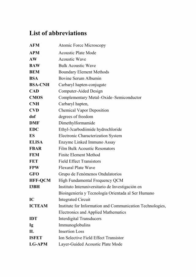
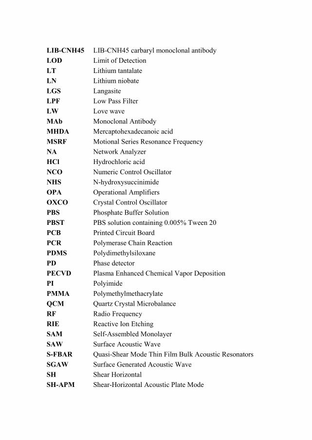
List of abbreviations
AFM Atomic Force Microscopy
APM Acoustic Plate Mode
AW Acoustic Wave
BAW Bulk Acoustic Wave
BEM Boundary Element Methods
BSA Bovine Serum Albumin
BSA-CNH Carbaryl hapten-conjugate
CAD Computer-Aided Design
CMOS Complementary Metal–Oxide–Semiconductor
CNH Carbaryl hapten,
CVD Chemical Vapor Deposition
dof degrees of freedom
DMF Dimethylformamide
EDC Ethyl-3carbodiimide hydrochloride
ES Electronic Characterization System
ELISA Enzyme Linked Immuno Assay
FBAR Film Bulk Acoustic Resonators
FEM Finite Element Method
FET Field Effect Transistors
FPW Flexural Plate Wave
GFO Grupo de Fenómenos Ondulatorios
HFF-QCM High Fundamental Frequency QCM
I3BH Instituto Interuniversitario de Investigación en
Bioingeniería y Tecnología Orientada al Ser Humano
IC Integrated Circuit
ICTEAM Institute for Information and Communication Technologies,
Electronics and Applied Mathematics
IDT Interdigital Transducers
Ig Immunoglobulins
IL Insertion Loss
ISFET Ion Selective Field Effect Transistor
LG-APM Layer-Guided Acoustic Plate Mode
LIB-CNH45 LIB-CNH45 carbaryl monoclonal antibody
LOD Limit of Detection
LT Lithium tantalate
LN Lithium niobate
LGS Langasite
LPF Low Pass Filter
LW Love wave
MAb Monoclonal Antibody
MHDA Mercaptohexadecanoic acid
MSRF Motional Series Resonance Frequency
NA Network Analyzer
HCl Hydrochloric acid
NCO Numeric Control Oscillator
NHS N-hydroxysuccinimide
OPA Operational Amplifiers
OXCO Crystal Control Oscillator
PBS Phosphate Buffer Solution
PBST PBS solution containing 0.005% Tween 20
PCB Printed Circuit Board
PCR Polymerase Chain Reaction
PDMS Polydimethylsiloxane
PD Phase detector
PECVD Plasma Enhanced Chemical Vapor Deposition
PI Polyimide
PMMA Polymethylmethacrylate
QCM Quartz Crystal Microbalance
RF Radio Frequency
RIE Reactive Ion Etching
SAM Self-Assembled Monolayer
SAW Surface Acoustic Wave
S-FBAR Quasi-Shear Mode Thin Film Bulk Acoustic Resonators
SGAW Surface Generated Acoustic Wave
SH Shear Horizontal
SH-APM Shear-Horizontal Acoustic Plate Mode
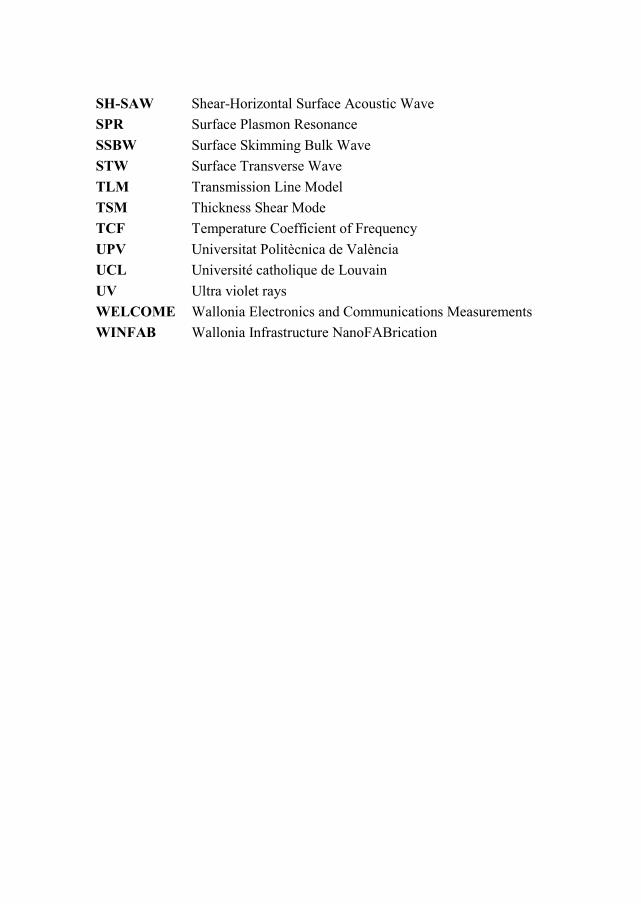
SH-SAW Shear-Horizontal Surface Acoustic Wave
SPR Surface Plasmon Resonance
SSBW Surface Skimming Bulk Wave
STW Surface Transverse Wave
TLM Transmission Line Model
TSM Thickness Shear Mode
TCF Temperature Coefficient of Frequency
UPV Universitat Politècnica de València
UCL Université catholique de Louvain
UV Ultra violet rays
WELCOME Wallonia Electronics and Communications Measurements
WINFAB Wallonia Infrastructure NanoFABrication

List of symbols
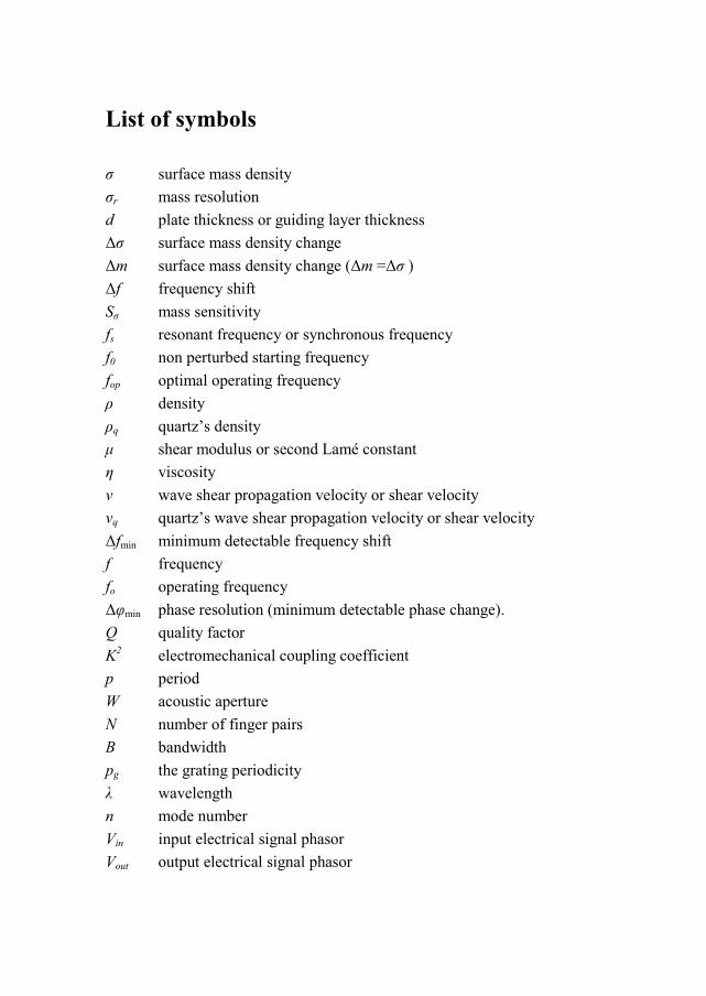
σ surface mass density
σr mass resolution
d plate thickness or guiding layer thickness
∆σ surface mass density change
∆m surface mass density change (∆m =∆σ )
∆f frequency shift
Sσ mass sensitivity
fs resonant frequency or synchronous frequency
f0 non perturbed starting frequency
fop optimal operating frequency
ρ density
ρq quartz’s density
µ shear modulus or second Lamé constant
η viscosity
v wave shear propagation velocity or shear velocity
vq quartz’s wave shear propagation velocity or shear velocity
∆fmin minimum detectable frequency shift
f frequency
fo operating frequency
∆φmin phase resolution (minimum detectable phase change).
Q quality factor
K2 electromechanical coupling coefficient
p period
W acoustic aperture
N number of finger pairs
B bandwidth
pg the grating periodicity
λ wavelength
n mode number
Vin input electrical signal phasor
Vout output electrical signal phasor
H(f) transfer function
φ phase-shift
vφ phase velocity, propagation velocity or wave velocity.
kLy guiding layer transverse wavenumber in y direction
vg group velocity
k wavevector
Zc characteristic impedance
vp particle velocity
TJ stress
Z impedance per unit of length
L inductance per unit of length
Y admittance per unit of length
C capacitance per unit of length
G conductance per unit of length
γ complex propagation factor
α attenuation coefficient
β phase coefficient
∇ ⋅ divergence
T stress vector
vp particle velocity vector
F external force vector
c matrix of elastic stiffness constants
c stiffness constant
S strain
S strain vector
θ complex coupling angle
αLW attenuation of the Love Wave
R response
M physical quantity to be measured
h coating layer thickness
ρC coating layer density
vSσ velocity mass sensitivity
vφ0 unperturbed phase velocity
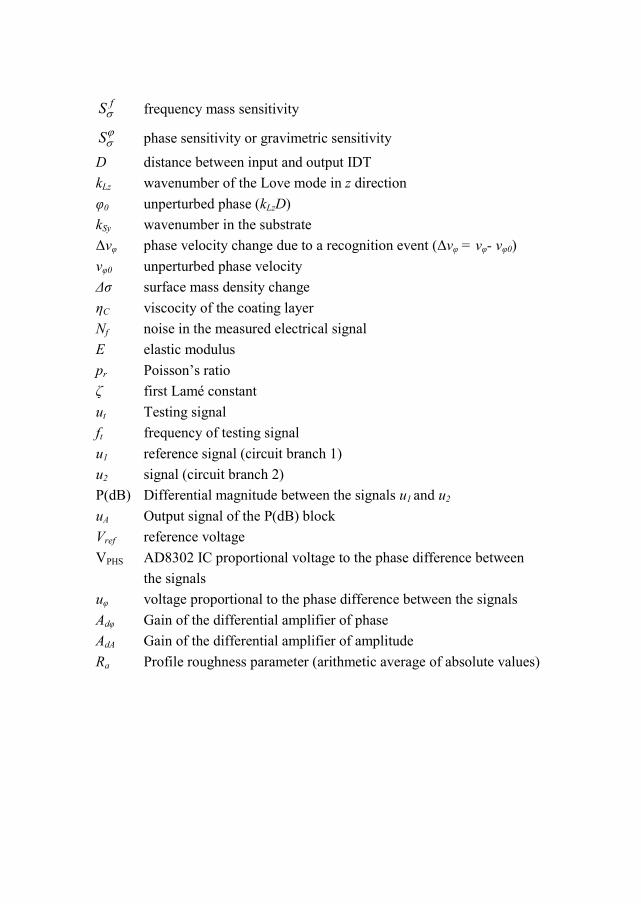
fSσ frequency mass sensitivity
Sϕσ phase sensitivity or gravimetric sensitivity
D distance between input and output IDT
kLz wavenumber of the Love mode in z direction
φ0 unperturbed phase (kLzD)
kSy wavenumber in the substrate
∆vφ phase velocity change due to a recognition event (∆vφ = vφ- vφ0)
vφ0 unperturbed phase velocity
∆σ surface mass density change
ηC viscocity of the coating layer
Nf noise in the measured electrical signal
E elastic modulus
pr Poisson’s ratio
ζ first Lamé constant
ut Testing signal
ft frequency of testing signal
u1 reference signal (circuit branch 1)
u2 signal (circuit branch 2)
P(dB) Differential magnitude between the signals u1 and u2
uA Output signal of the P(dB) block
Vref reference voltage
VPHS AD8302 IC proportional voltage to the phase difference between
the signals
uφ voltage proportional to the phase difference between the signals
Adφ Gain of the differential amplifier of phase
AdA Gain of the differential amplifier of amplitude
Ra Profile roughness parameter (arithmetic average of absolute values)

Index 1. Introduction ............................................................................................ 7
1.1 Context of research ........................................................................ 8
1.2 Biosensors .................................................................................... 11
1.2.1 Immunosensors .................................................................... 13
1.2.2 Immunoassay formats .......................................................... 14
1.2.3 Steps for the development of immunosensors ..................... 16
1.3 Sensing technologies for biochemical sensors ............................. 20
1.4 Why Acoustic? ............................................................................. 22
1.5 Acoustic Wave devices ................................................................ 23
1.5.1 Quartz Crystal Microbalance (QCM)................................... 27
1.5.2 Thin film bulk acoustic resonators (FBAR) ......................... 30
1.5.3 Rayleigh wave (SAW) ......................................................... 32
1.5.4 Shear-Horizontal Surface Acoustic Wave (SH-SAW)......... 33
1.5.5 Surface Transverse Wave (STW)......................................... 35
1.5.6 Love wave (LW) .................................................................. 37
1.5.7 Shear-Horizontal Acoustic Plate Mode (SH-APM) ............. 38
1.5.8 Layer-Guided Acoustic Plate Mode (LG-APM) .................. 40
1.5.9 Flexural Plate Wave (FPW) ................................................. 40
1.5.10 Performance comparison ...................................................... 42
1.6 LW biosensors state-of-the-art ..................................................... 47
1.7 Trends and challenges of LW biosensors .................................... 50
2. Thesis objectives .................................................................................. 53
3. Contribution 1: LW sensor fundamentals. Optimization of the design specifications................................................................................................ 57
3.1 Introduction .................................................................................. 57
3.2 Basic structure .............................................................................. 58
3.2.1 Piezoelectric substrate .......................................................... 60
3.2.2 Interdigital transducers (IDTs) ............................................. 62
3.2.3 Guiding layer ....................................................................... 65
3.2.4 Sensing area ......................................................................... 67
3.3 Measurement techniques .............................................................. 68
3.4 Modeling methods ....................................................................... 72
3.4.1 Dispersion equation.............................................................. 72
3.4.2 Transmission line model ...................................................... 75
3.4.3 3D FEM simulations ............................................................ 90
3.4.4 Sensitivity and Limit of Detection ....................................... 95
3.5 Studies to define other design specifications ............................... 99
3.5.1 Temperature effect: Selection of the substrate material ....... 99
3.5.2 Optimum guiding layer material and thickness for maximum sensitivity ........................................................................................... 102
3.5.3 Reflectors for enhancing the device response .................... 106
3.5.4 Packaging and flow cells .................................................... 108
3.6 Chapter conclusion ..................................................................... 110
4. Contribution 2: Fabrication and characterization of the LW sensor .. 115
4.1 Introduction ................................................................................ 115
4.2 Structure and dimensions of the sensors .................................... 116
4.3 Fabrication of the sensors .......................................................... 119
4.3.1 IDTs patterning .................................................................. 119
4.3.2 Silicon dioxide guiding layer PECVD deposition ............. 120
4.3.3 Opening of the contacts ...................................................... 121
4.3.4 Gold sensing layer deposition ............................................ 121
4.4 Characteristics of the fabricated sensors .................................... 122
4.4.1 Atomic Force Microscopy (AFM) images ......................... 123
4.4.2 Frequency response of the final sensors ............................. 125
4.4.3 Theoretical mass sensitivity ............................................... 126
4.5 Chapter conclusion ..................................................................... 129
5. Contribution 3: LW microsystem for in liquid measurements ........... 131
5.1 Design and fabrication of a flow cell for the LW sensor ........... 132
5.2 Electronic characterization system ............................................. 140
5.2.1 Electronic characterization system for QCM resonators.... 142
5.2.2 Electronic characterization system for LW sensors ........... 148
5.3 Proposed characterization system vs. a reference instrument .... 153
5.4 Chapter conclusion ..................................................................... 155
6. Experimental section .......................................................................... 157
6.1 Introduction ................................................................................ 157
6.2 Experiment 1: Measurements of glycerol-water solutions ......... 158
6.2.1 Materials and Methods ....................................................... 158
6.2.2 Results and discussion ....................................................... 162
6.3 Experiment 2: Carbaryl immunosensor ..................................... 165
6.3.1 Materials and methods ....................................................... 166
6.3.2 Results and discussion ....................................................... 173
6.4 LW sensors versus HFF-QCMs ................................................. 187
6.5 Chapter conclusions ................................................................... 189
7. Final conclusions ............................................................................... 191
Appendix A. Lamé constants ..................................................................... 195
Appendix B. Euler angles .......................................................................... 197
Appendix C. Crystal cuts and IEEE standard 176 on piezoelectricity ....... 199
Appendix D. Material properties for LW sensors ...................................... 203
Appendix E. Scattering Parameters ........................................................... 211

Appendix F. Finite Element Method formulation ...................................... 215
Appendix G. Thesis codes ......................................................................... 223
List of scientific communications .............................................................. 227
References .................................................................................................. 229
María Isabel Rocha Gaso
5
Foreword
This dissertation is divided into the following chapters:
In Chapter 1, the necessity of improving the sensitivity and limit of detection of current acoustic devices is established. The High Fundamental Frequency Quartz Crystal Microbalance (HFF-QCM) is considered as the first option to achieve this. The development of such devices and their required instrumentation is performed in a parallel dissertation. As a second option, another acoustic wave technology is considered as an alternative of the HFF-QCM. Therefore, different acoustic wave devices for biosensing applications are reviewed and their structure, materials, operation frequency, reported sensitivity, advantages and disadvantages are studied. Love Wave sensors are identified as promising and robust devices for biosensing. Hence, the manuscript provides the state-of-the-art of Love Wave biosensors. Finally, the trends and challenges these devices currently face for being applied as biosensors have been mentioned.
The information gathered in Chapter 1 helps to establish the Thesis objectives mentioned in Chapter 2.
Chapter 3 provides the Love wave sensor fundamentals and analysis of the current state-of-the-art elements that composed them, as well as the common measurement techniques. It also describes the most commonly used methods for modeling Love Wave devices. All the information gathered in the first part of this chapter serves as an introduction to the first Thesis contribution, which is presented at Section 3.5. This section describes the results of some studies that were performed in order to establish optimized design specifications for the final device, which was going to be fabricated.
Chapter 4 presents the fabrication process and characterization of the final device.
Since biosensing applications were targeted, where the operation in liquid media is required, it was necessary to implement a flow-through cell for the fabricated sensor. Chapter 5 mentions the requirements of flow cells for Love Wave sensors and explains the design and fabrication of the flow cell. In addition, this chapter describes an electronic characterization system
1. Introduction
6
for Love Wave sensors, based on a previous electronic characterization system developed for QCM sensors. The most similar possible measurement system for Love Wave sensors and QCM were sought in order to compare these technologies under similar conditions for a reliable comparison.
Chapter 6 corresponds to the experimental section of the Thesis, which was performed to validate the Thesis contributions for biosensing applications. The materials, methods, results and discussion of the following two experiments:
• Experiment 1: Measurements of glycerol-water solutions and
• Experiment 2: Carbaryl immunosensor are presented. Experiment 1 was carried out for determining the reliability and accuracy of the implemented characterization system. Experiment 2 was carried out to validate the developments of this Thesis for biosensing applications. This chapter presents a table comparing the results obtained with the developed carbaryl Love wave immunosensor and other carbaryl detection technologies like SPR and ELISA. Finally, this chapter provides a comparison between Love wave sensors and HFF-QCMs.
Chapter 7 mentions the dissertation conclusions. In addition, some future lines are included; some of them are currently being investigated in our research group.
María Isabel Rocha Gaso
7
1. Introduction
In the fields of medical diagnosis, drug discovery, biotechnology and environmental monitoring faster, more selective and more sensitive results are being demanded. Pathogen agents, such as bacteria, fungi and viruses are found widely in the environment, food, marine and estuarine waters, soil and the intestinal tracts of humans and animals. Many of these organisms have an essential function in nature, but certain potentially harmful micro-organisms can have profound negative effects on both animals and humans, costing the food industry (and indirectly, the consumers) many millions of dollars each year [2]. It is estimated that infectious diseases cause about 40% of the approximately 50 million total annual deaths world-wide [3]; waterborne pathogens cause 10-20 million of these deaths and, additionally, more than 200 million people suffer non-fatal infections each year [4].
Microbial and viral identification, and quantification assays usually rely on conventional approaches of plating and incubation method on culture media, as well as on biochemical testing, microscopy, etc. Over the last 20 years, many new methods have been developed, including immunological methods, polymerase chain reaction (PCR) and biosensors [5]. PCR, although very specific and suitable for screening purposes, still fails to produce accurate results when enumeration of viable cells is needed [6]. Further efforts are being made, for making conventional PCR systems faster, more efficient, and low cost [7].
Pesticides are biocides by definition, and thus, they are potentially harmful for humans and the environment [8]. The traditional chromatographic analysis (liquid or gas chromatography) is a standardized technique which is highly sensitive and allows detecting many compounds of the same family simultaneously. Chromatography is the most widely used method for the determination of pesticides. However, the main disadvantage of this laborious analysis is that it has to be realized in well-equipped
1. Introduction
8
centralized laboratories. During the last decades, increasing awareness about the presence of pesticide residues in the environment has been urging the search for simple and effective detection methods [9]. Due to the potential threat of pesticides to human health, the European Union has established the limit concentration allowable in water intended for human consumption to 0.10 µg/L for each individual pesticide.
Biosensors offer a great potential for achieving more rapid, sensitive, selective, portable, power-efficient and low costs methods of detecting pathogen, molecules and other potentially harmful compounds, like pesticides and biochemical warfare agents [10]. A reduction of costs and analysis time is possible with modern biosensors [11].
In this Thesis the detection of a low molecular weight compound, carbaryl pesticide, is pursued. Carbaryl was chosen as a model analyte, since these other detection technologies (acoustic and non-acoustic) have been widely used for the detection of this analyte. Carbaryl, an acetyl-cholinesterase inhibitor, is a broad-spectrum N-methyl carbamate insecticide and it is widely used around the world [8]. Although some adverse effects have been reported, like possible disruption of the nervous-system functions [12], it is considered a safe insecticide because of its low toxicity in mammals [13]. Nevertheless, carbaryl has been reported as a neurotoxin with toxicity close to some chemical warfare agents [14].
1.1 Context of research
The research group Grupo de Fenómenos Ondulatorios (GFO) of the Universitat Politècnica de València (UPV) has a great experience in the physical background and read-out circuitry for Quartz Crystal Microbalance (QCM) sensors. Since 2002, GFO, in collaboration with the group of the Instituto Interuniversitario de Investigación en Bioingeniería y Tecnología Orientada al Ser Humano (I3BH) have developed three previous Spanish National Projects directly related to the use of QCM for biosensors:
1) Desarrollo de inmunosensores piezoeléctricos para la detección de
plaguicidas N-metil carbamatos y organophosphorades en alimentos y
bacterias lácticas en la cerveza (Reference: AGL2002-01181).
María Isabel Rocha Gaso
9
2) Desarrollo de un inmunosensor piezoeléctrico multi-residuo para la
detección de plaguicidas en agua y alimentos (Reference: AGL2006-12147/ALI)
3) Inmunosensor piezoeléctrico de alta frecuencia para la detección de
ftalatos y el bisfenol A en alimentos envasados (Referene: AGL2009-13511/ALI).
In the first project, a piezoelectric immunosensor for the detection of Carbaryl pesticide using a 9 MHz-QCM device was achieved, including the read-out circuitry and flow-cell. This immunosensor had a sensitivity of 30 µg/L and a LOD of 11 µg/L [9]. The second project was proposed with the aim to improve the traditional QCM device sensitivity and mass resolution for the detection of pesticide in water and food. The main objective was to increase the fundamental working frequency of QCM sensors moving towards a High Fundamental Frequency QCM (HFF-QCM ) system. During the development of this project, two main technological hindrances were found: 1) the fragility of HFF-QCM devices, since increasing the frequency in AT-cut quartz sensors always implies decreasing thickness, and, 2) the instability of the employed high frequency electronic characterization system. With the aim to solve these hurdles, GFO initiated two new research lines: 1) searching for new technologies which solve the fragility issue of QCM devices, which resulted in a study of the state-of-the art of other acoustic wave devices and in the selection of LW technology as a good candidate and 2) the proposal of a new concept for the sensor characterization method, which consisted of a continuous tracking of the sensor phase-shift when it was excited to a fixed frequency, instead of the traditional one based on a continuous tracking of the sensor frequency. These two lines initiated in these projects continued in the development of this Thesis and a parallel one regarding HFF-QCM with fundamental frequencies between 50 and 150 MHz. The success of these three mentioned projects provided a convenient background for the team to face the goal pursued in both Theses.
This parallel work will be profited to compare both technologies (LW and HFF-QCM) under the same conditions. Such comparison will elucidate the real advantages and disadvantages of each technology for a specific application.
1. Introduction
10
The opening of this new research line on LW technology in the GFO would not had been possible without the support of the Institute for Information and Communication Technologies, Electronics and Applied Mathematics (ICTEAM) at the Université catholique de Louvain (UCL), Belgium. This institution jointly supervised this Thesis. The Sensors, Microsystems and Actuators Laboratory of Louvain (SMALL) of the ICTEAM Institute, which participated in this Thesis, has, among others, the following research interests:
• MEMS and NEMS sensors and actuators for biomedical, environmental and aeronautics/space applications: engineering and teaching of micro- and nano-electromechanical device (design, fabrication, characterization, reliability and packaging).
• Integration of thin-film functional materials in microsensors: ultrananocrystalline diamond, piezoelectric materials, sensing (bio)chemical layers, etc.
• Acoustic wave devices for sensors (SAW and FBAR).
The ICTEAM is equipped with two main state-of-art technological platforms: WINFAB and WELCOME, some of the most advanced laboratories in the world (see facilities in chapter 4), which were ideal for the fabrication of LW sensors. The PhD student, who presents this Thesis, received the necessary training and support in this institution for the fabrication of LW sensors during a one-year research stay.
The collaboration between the described research groups has been essential for the successful development of this Thesis. This collaboration generated a multidisciplinary, international and high-level work environment, which was very helpful for overcoming the technical challenges that emerged when opening this new research line. These challenges are not always published in the literature.
Next, the fundamentals of biosensors and immunosensors are introduced. Later, a brief description of the most popular sensing technologies for biochemical sensors (electrochemical, optical and acoustic wave) is presented. Afterwards, the chapter explains the reasons why the acoustic wave technology is preferred for the development of this Thesis. Finally, the acoustic wave devices applied for biosensing are described and
María Isabel Rocha Gaso
11
compared with the purpose of determining the most promising device for these applications.
1.2 Biosensors
The term ‘‘biosensor’’ began to appear in the scientific literature in the late 1970s [15]. The National Research Council (NRC) defines a biosensor as a
detection device that incorporates a) a living organism or product derived
from living systems (e.g., an enzyme or an antibody) and b) a transducer to
provide an indication, signal, or other form of recognition.
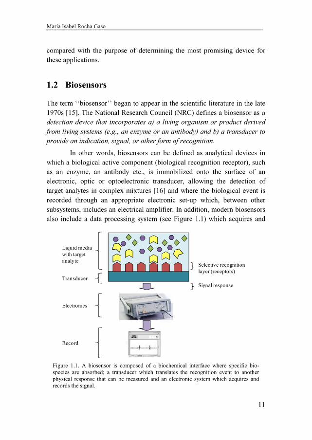
In other words, biosensors can be defined as analytical devices in which a biological active component (biological recognition receptor), such as an enzyme, an antibody etc., is immobilized onto the surface of an electronic, optic or optoelectronic transducer, allowing the detection of target analytes in complex mixtures [16] and where the biological event is recorded through an appropriate electronic set-up which, between other subsystems, includes an electrical amplifier. In addition, modern biosensors also include a data processing system (see Figure 1.1) which acquires and
Figure 1.1. A biosensor is composed of a biochemical interface where specific bio-species are absorbed; a transducer which translates the recognition event to another physical response that can be measured and an electronic system which acquires and records the signal.
Transducer
Liquid media with target analyte
Selective recognition layer (receptors)
Signal response
Electronics
Record
1. Introduction
12
records the signals [11]. Since the objective of biosensing is the successful characterization of biomolecular interactions in their natural liquid environment, a fluidic or microfluidic system is also required to contain the fluids to be analyzed, lead them to the sensing area and dispatch them. A fluidic system includes pipes, pumps, valves and a liquid cell or flow-
through cell, which makes the system very complex. Therefore, advances in biosensing can be achieved by efforts in four main fields: the transduction mechanism, the biological reception mechanism (sensitive film), (micro)fluidics and characterization systems. This fact makes biosensing highly interdisciplinary.
Some applications of biosensors include personal glucose testing for diabetics, DNA & RNA sensing, cancers and HIV detection, immunological reactions, cell adhesion, adsorption and hybridization of oligonucleotides, characterization of adsorbed proteins and bacteria, virus and pesticides detection, among others. Thus, the potential market for biosensors is known to be very large. However, the commercialization of numerous biosensors has been slow, except for glucose monitoring [11].
Ideal biosensors should be fast, easy to use, specific, reliable, and inexpensive. Additionally, they should allow real-time direct monitoring and miniaturized devices. Miniaturization is going to be a key consideration while developing biosensors [17], since high performance miniature biosensors are not only expected to quicken commercialization but will also allow biosensors to penetrate several unexploited markets. In this sense, with the move toward miniaturization and developments in lab-on-a-chip technologies, participants that can offer refined products to meet the expanding biosensor applications are set to gain a competitive edge [17]. The development hindrances of biosensors has been imposed by a lack in their desired performance characteristics in terms of sensitivity, dynamic range and reproducibility [11]. Furthermore, some biosensor technologies require to deep in research before the technology can be transferred, and in many cases the involved research projects comprise long gestation periods with low success rates [17]. However, what still makes biosensor technology extremely attractive and a serious alternative to other well established techniques are aspects, such as the minimal sample preparation, high speed of analysis and the potential for in situ and flow stream analysis for process control [17,18].
María Isabel Rocha Gaso
13
Next, a specific type of biosensor, called immunosensor, will be described, since an immunosensor for the detection of carbaryl pesticide will be used as a validation model in this Thesis.
1.2.1 Immunosensors
An immunosensor is a particular type of a biosensor in which the biological component that detects the target analyte is an immunoreagent involved in an immunoassay [19]. An immunoassay is every analytical procedure based on a specific antigen-antibody recognition [16,20]. Generally, only one antibody takes part in the immunoassay, whereas several antigens can be involved in the reaction (free analytes, protein-haptens conjugate, etc.) [16].
Immunological detection with antibodies is perhaps the most successful technology employed for the detection of cells, spores, viruses and toxins alike [21]. Moreover, immunoassays can be performed on portable devices, irrespective of centralized laboratories, which turn them into a suitable tool for quantification analysis in on-line applications.
Nowadays, Enzyme Linked Immuno Assay (ELISA) and immunosensors are the most popular immunoassays [19]. In ELISAs the detection of the analyte is always indirect since one of the immunoreagents is labeled with an enzyme. During the last step of this assay, a colorimetric signal is produced when the enzyme transforms a colorless substrate into a colored product [16]. In those techniques, where labels are necessary, the actual quantitative measurement is only done after the bio-chemical recognition step, which is a disadvantage. Moreover, the label can compromise the bio-chemical activity [22].
In immunosensors, the detection is direct, one of the immunoreagents is immobilized on the surface of the transducer and a direct physical signal is produced when the interactions occur [16,23,24]. Label-free detection (direct detection) represents an essential advantage of immunosensors as compared to label-dependent immunoassays (indirect detection) like ELISA [25].
Immunosensors combine the selectivity provided by immunological interactions with the high sensitivity achieved by the signal transducers and they have proven to be powerful analytical devices for the monitoring of
1. Introduction
14
low molecular weight compounds, such as organic pollutants in food and the environment [26,27]. However, lower sensitivity is obtained with immunosensors compared to ELISA.
Piezoelectric immunosensors use a piezoelectric substrate as a transducer element, working in the microgravimetric mode. The most commonly employed piezoelectric immunosensor use the Quartz Crystal
Microbalance (QCM) as the transducer. QCM is a mature and robust technique. However, in recent years, piezoelectric immunosensors based on Surface Generated Acoustic Wave (SGAW) devices have emerged as a powerful technology [10]. The gold electrodes of piezoelectric immunosensors are used as a support for the immobilization of immunoreagents, in such a way that subsequent immunoreactions can be detected as a mass variation and correlated with the concentration of the analyte [16]. One of the main advantages of piezoelectric immunosensors over other techniques like ELISA is the reusability. Piezoelectric immunosensors can be reused for at least 150 assay cycles, without no significant loss of sensitivity [9].
In next section, different formats of immunoassays are described.
1.2.2 Immunoassay formats
Antibody molecules belong to the family of proteins known as immunoglobulins (Ig) which are subdivided into five classes: IgG, IgM, IgA, IgE and IgD [28]. They are produced naturally by the immune system of mammals, as a reaction against the exposure to an external agent (antigen). Antibodies can also be produced in laboratories to lately be employed in analytical processes.
Small organic (low molecular weight) molecules, such as pesticides, drugs, etc., are generally not recognized for the immune system as immunogenic molecules (non immunogenic). Thus, they do not elicit any immune response when introduced in experimental mammals. Therefore, these types of analytes acquire immunogenicity only after being conjugated to a carrier molecule. Then, in order to generate antibodies, the synthesis of chemically modified analytes and their covalent binding to proteins are required. Haptens are chemically modified analytes which introduce in their
María Isabel Rocha Gaso
15
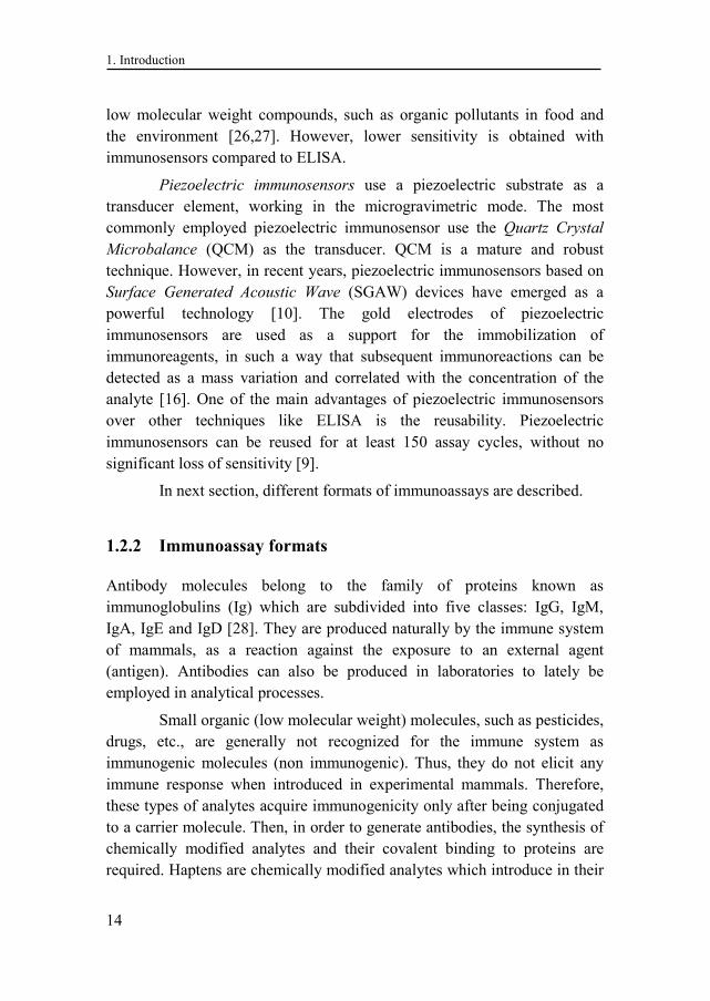
structure the chemical groups suitable for protein conjugation. The union hapten plus carrier protein is called hapten-conjugate. The hapten conjugate is used as the antigen to immunize the animals and also as the assay conjugate in immunoassays.
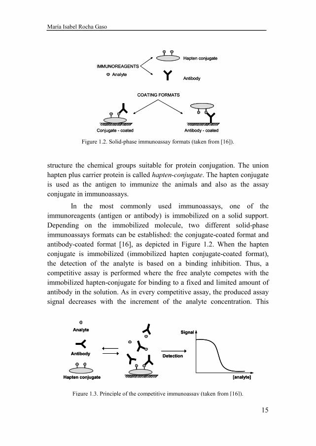
In the most commonly used immunoassays, one of the immunoreagents (antigen or antibody) is immobilized on a solid support. Depending on the immobilized molecule, two different solid-phase immunoassays formats can be established: the conjugate-coated format and antibody-coated format [16], as depicted in Figure 1.2. When the hapten conjugate is immobilized (immobilized hapten conjugate-coated format), the detection of the analyte is based on a binding inhibition. Thus, a competitive assay is performed where the free analyte competes with the immobilized hapten-conjugate for binding to a fixed and limited amount of antibody in the solution. As in every competitive assay, the produced assay signal decreases with the increment of the analyte concentration. This
Figure 1.2. Solid-phase immunoassay formats (taken from [16]).
AntibodyAnalyte
Hapten conjugate
IMMUNOREAGENTS
Antibody - coatedConjugate - coated
COATING FORMATS
AntibodyAnalyte
Hapten conjugate
IMMUNOREAGENTS
Antibody - coatedConjugate - coated
COATING FORMATS
Figure 1.3. Principle of the competitive immunoassay (taken from [16]).
Antibody
Analyte
Hapten conjugate
Detection
Signal
[analyte]
Antibody
Analyte
Hapten conjugate
Detection
Signal
[analyte]
1. Introduction
16
inversely proportional relationship, between analyte concentration and immunosensor signal, produces the typical competitive immunoassay standard curves in Figure 1.3. For the detection of low molecular weight compounds this immunoassay format is recommended, because the binding of the antibody to the immobilized hapten-conjugate produce a greater mass change in the surface of the device. On the other hand, the immobilized antibody format is not recommended for immunoassays in which a regeneration of the sensor is required, since the substances used for the immunoassay can modified the antibody chemical structure and render it inactive. In addition, antibody-coated formats require a complicate immobilization procedure involving antibody orientation strategies [12]. Furthermore, antibodies are less stable to temperature changes.
The development of immunosensors requires an extensive previous work regarding the production and immobilization of immunoreagents. In next epigraphs, a brief description of the steps required to achieve an immunosensor is provided.
1.2.3 Steps for the development of immunosensors
The required steps for the development of immunosensors are the following:
a) Hapten synthesis. b) Monoclonal antibody production. c) Immobilization of immunoreagents. d) Characterization of the immunosensor.
a) Hapten synthesis
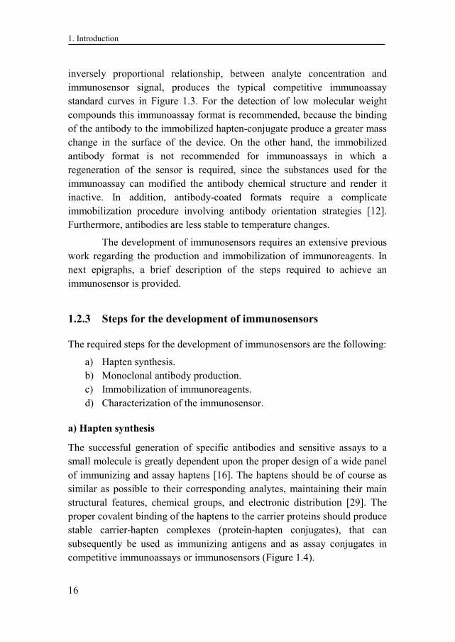
The successful generation of specific antibodies and sensitive assays to a small molecule is greatly dependent upon the proper design of a wide panel of immunizing and assay haptens [16]. The haptens should be of course as similar as possible to their corresponding analytes, maintaining their main structural features, chemical groups, and electronic distribution [29]. The proper covalent binding of the haptens to the carrier proteins should produce stable carrier-hapten complexes (protein-hapten conjugates), that can subsequently be used as immunizing antigens and as assay conjugates in competitive immunoassays or immunosensors (Figure 1.4).
María Isabel Rocha Gaso
17
Hapten design is a key step in the development of immunoassays for small molecules, since the hapten is primarily responsible for determining the antibody recognition properties.
b) Monoclonal antibody production
Immunoassays development requires the production of antibodies for the analytes and their incorporation into adequate assay configurations. As mentioned before, the successful development of specific antibodies and sensitive assays to small molecules greatly depends on a proper design of haptens.
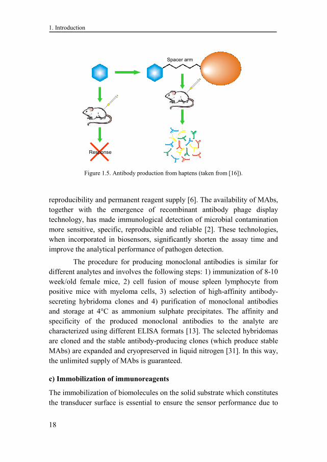
The preparation of antibodies against haptens, designed for special applications, such as pesticides, is based on covalent binding of the hapten to a carrier protein followed by immunization of animals with the synthesized immunogens, as depicted in Figure 1.5. The chemical binding of the hapten to a protein determines in part the antibody specificity [30].
Once the immunogens for the analyte are prepared, the debate arises whether polyclonal or monoclonal antibodies will be obtained [16]. Polyclonal antibodies are produced by using traditional immunization procedures, mostly in rabbits, goats, sheep and pigs. These antibodies are widely used as reagents in many immunochemical analyses. Although, a major disadvantage of this approach lies in the fact that it is not possible to produce identical antibody specificity even in two animals of the same species. Polyclonal antibodies can be raised quickly and cheaply but they are often unspecific and available in limited amounts. In contrast, Monoclonal Antibodies (MAbs) have the advantage of ensuring
Figure 1.4. Preparation of immunogenic conjugates from low-molecular weight analytes (taken from [16]).
Protein
Analyte Hapten
X
Immunogen
(Hapten-Conjugate)
Protein
Analyte Hapten
X
Immunogen
(Hapten-Conjugate)
1. Introduction
18
reproducibility and permanent reagent supply [6]. The availability of MAbs, together with the emergence of recombinant antibody phage display technology, has made immunological detection of microbial contamination more sensitive, specific, reproducible and reliable [2]. These technologies, when incorporated in biosensors, significantly shorten the assay time and improve the analytical performance of pathogen detection.
The procedure for producing monoclonal antibodies is similar for different analytes and involves the following steps: 1) immunization of 8-10 week/old female mice, 2) cell fusion of mouse spleen lymphocyte from positive mice with myeloma cells, 3) selection of high-affinity antibody-secreting hybridoma clones and 4) purification of monoclonal antibodies and storage at 4°C as ammonium sulphate precipitates. The affinity and specificity of the produced monoclonal antibodies to the analyte are characterized using different ELISA formats [13]. The selected hybridomas are cloned and the stable antibody-producing clones (which produce stable MAbs) are expanded and cryopreserved in liquid nitrogen [31]. In this way, the unlimited supply of MAbs is guaranteed.
c) Immobilization of immunoreagents
The immobilization of biomolecules on the solid substrate which constitutes the transducer surface is essential to ensure the sensor performance due to
Figure 1.5. Antibody production from haptens (taken from [16]).
Spacer arm
Response
Spacer arm
Response
María Isabel Rocha Gaso
19
its role in the specificity, sensitivity, reproducibility and recycling ability. Some of the requirements that should be fulfilled by an immobilization process are the following [16]: 1) retention of biological activity of biomolecules after immobilization onto the sensor surface; 2) reproducible, durable and stable attachment with the substrate against variations of pH, temperature, ionic strength and chemical nature of the microenvironment and 3) uniform, dense and oriented localization of the biomolecules.
Several methods to immobilize biomolecules have been reported in literature. They include physical adsorption [27,32], avidin-biotin system [33] and covalent binding [33-37]. Among them, covalent binding is the most promising technique since it fulfills most of the requirements mentioned previously. Covalent immobilization assures a reproducible, durable and stable attachment to the substrate against physico-chemical variations in the aqueous microenvironment.
Lately, great effort has been committed to the achievement and optimization of conditions for covalent binding. Self-Assembled Monolayer (SAM) technology is providing the best results [12,38-42]. SAM is the generic name given to the methodologies and technologies that allow the generation of monomolecular layers (monolayers) of biological molecules on various substrates. The formation of such monolayer systems is extremely versatile, allowing the in vitro development of bio-surfaces which are able to mimic naturally occurring molecular recognition processes [16].
Gold surfaces allow the use of functionalized thiols, whereas SiO2 surfaces enable the use of various silanes [16]. Both methods produce monolayers of active groups for the subsequent coupling of biomolecules onto the transducer surface. However, since no single immobilization method has proven to be optimum for all possible transducers [3], suitable immobilization methods have to be developed for every combination of biological reagent and sensor surface.
The following step in the immunosensor development is its characterization.
d) Characterization of the immunosensor
The characterization process strongly depends on the chosen immunoassay format. Next, this process will be described for the immunoassay format
1. Introduction
20
(immobilized hapten-conjugate-coated format) employed in this Thesis. The reason why this format was selected is that the regeneration of the sensor was desired and the detection of a low molecular weight compound was looked for.
The data obtained with the assay setup are stored and processed in order to obtain the corresponding competitive curve. This curve is adjusted to a determined mathematic model, i.e. a sigmoidal function. The calibration curve then, allows the analysts to calculate the analyte concentration, sensitivity and limit of detection of the assay. The analyte concentration which reduces the assay signal to 50% of the maximum signal (which is obtained in the absence of analyte in the solution) is known as the I50. This value is generally accepted as an estimate of the immunosensor sensitivity, in such a way that the lower the I50 value, the higher the assay sensitivity [16]. In the same way, using this curve, the limit of detection it is obtained when the analyte concentration provides 90% of the maximum signal. The maximum signal is also used to determine the sensor reusability. A sensor can be reused, after a regeneration cycle with hydrochloric acid, when there is only a slight reduction of the maximum signal and, then, there is not a significant loss of sensitivity.
1.3 Sensing technologies for biochemical sensors
Different sensing technologies are being used for biochemical sensors. Classified by the transducer mechanism, electrochemical, optical and acoustic wave sensing technologies have emerged as the most promising biochemical sensor technologies. Common to most optical and electrochemical principles is the requirement of a label, like in the case of ELISAs, which increases the complexity and thus the cost of the analysis.
Electrochemical sensing is a well established technology. Using the reaction taking place at the interface of an electronic conductor and an ionic conductor there are devices operating in potentiometric or amperometric modes. Most of electrochemical sensors are based on an enzymatic reaction with the chemical species to be detected; for that, an appropriate enzyme must be immobilized on top of an electrode. Amperometric devices are the most prevalent and commercialize examples for glucose and lactic acid [43].
María Isabel Rocha Gaso
21
Field Effect Transistors (FET) can also be used for electrochemical sensing after modifying their structure. Chemical species can be monitored by the field induced current variation in the transistor channel if an appropriate recognition layer is added to the gate dielectric to provide chemical specificity [44]. This is the principle of the Ion Selective Field
Effect Transistor (ISFET). ISFETs can be used for bio-chemical sensing when a sensitive coating is deposited on the surface or can be associated with enzymatic reactions [44,45]. Miniaturization is the main advantage of the FET sensors; they can be integrated into arrays, allowing multiple measurands to be detected with one device. They are manufactured by CMOS technology making them very cheap. However, the ISFETs also need a reference potential sensing electrode to function properly, which is difficult to integrate close to the interface.
Optical sensing represents the most often technology currently used in biochemical applications. Mechanisms in optical sensing include interferometry, infrared absorption, scattering, luminescence and polarimetry. Optical sensors can be very sensitive, but tend to be quite expensive compared to other sensing technologies [45,46]. Among them, Fluorescence and Surface Plasmon Resonance (SPR) are probably the best known optical techniques. Fluorescence is one of the most sensitive techniques [47], but requires labeling and very complicated read-out systems. This is one of the limiting factors of its integration with electronics in a simple device. SPR sensors detect changes in the refractive index of a layer after the bio-chemical reaction occurs on it. This is done by detecting the angle of minimum reflection intensity of a laser or LED pointed at the layer. SPR sensors can be label free, but the shortcoming of this method is that they require a light source, and it cannot be configured easily for high throughput detection. Moreover, the SPR technique depends on the optical properties of the employed materials. They are easier to be integrated than fluorescent sensors but the optical parts remain as the main problem. SPR has become a well established method suitable for the direct on-line detection of immunological reactions [48]. The commercialized Spreeta sensors, from Texas Instruments Inc., with very high sensitivities are compatible with many receptor coatings [49].
Acoustic Wave (AW) sensors operate with mechanical elastic waves as the transduction mechanism. Acoustic sensing has taken advantage of the
1. Introduction
22
progress made in the last decades in piezoelectric resonators for radio-frequency (RF) telecommunication technologies. The piezoelectric elements used in radars, cellular phones or electronic watches for the implementation of filters, oscillators, etc., have been applied to sensors [50]. The gravimetric technique, first reported by Sauerbrey in 1959 [51], is based on the change in the resonance frequency experimented by the resonator due to a mass attached on the sensor surface. This technique opened a great deal of applications in bio-chemical sensing in both gas and liquid media.
During the next sections an insight into the acoustic technology will be provided, since this is the sensing technology which will be employed during this work. In next section an explanation of why this technology is preferred among others is given.
1.4 Why Acoustic?
Most of the biochemical interactions, described in Section 1.2, are susceptible of being evaluated and monitored in terms of mass transfer over the appropriate interface. This characteristic allows using the gravimetric techniques based on acoustic sensors for a label-free and a quantitative time-dependent detection. Optical biosensors can be very sensitive, but tend to be quite expensive compared to other sensing technologies [46]. Piezoelectric
Acoustic Wave devices represent a cost-effective alternative [9]. Acoustic sensor based technologies combine their direct detection, real-time monitoring, high sensitivity and selectivity capabilities with a reduced cost. As mentioned previously, the SPR technique depends on the optical properties of the employed materials. On the contrary, the most applied principle of detection in acoustic sensing for bio-chemical applications is based on mass (gravimetric) properties, being independent of the optical materials' properties. This allows performing studies over a great variety of surfaces making it suitable for direct measurement on crude, unpurified samples [22], eliminating the need of sample preparation (as it occurs in liquid or gas chromatography). Therefore, the number of steps involved in the process is reduced – bringing many benefits, including significant time and cost-savings–. Additionally, acoustic systems provide information on the real binding to a receptor and not simply proximity to a receptor, as it occurs in SPR techniques [22]. Furthermore, the key measuring magnitudes
María Isabel Rocha Gaso
23
of acoustic wave devices are the frequency, magnitude and/or phase of a signal, which can be processed easily and precisely.
Another attractive feature of acoustic technology is its portability which makes it suitable for applications where an in-situ and real-time monitoring of the sample is required. This avoids sending the sample to centralized laboratories reducing time and cost of the sample analysis. The miniaturization of the sensor itself and the sensor’s characterization system can greatly improve portability. In this sense, given that the wavelength of acoustic waves in solids is approximately 100 000 times smaller than the wavelength of electromagnetic waves at the same frequency, the possibility for true microminiaturization arises if appropriate elastic acoustic wave electronic circuitry can be devised [52].
The reasons why the acoustic wave technology was chosen among others for the development of this Thesis, were mentioned in this section. Next, a brief explanation of the most important aspects and most employed devices of this technology is provided. The operation principle and key features of each acoustic wave device are described, as well as its suitability for certain sensing applications.
1.5 Acoustic Wave devices
Acoustic Wave (AW) devices are sensitive to mechanical perturbations, temperature changes and electrical perturbations, such as pH changes, conductivity and dielectric permittivity of added materials [53]. These electrical effects can be reduced letting the device be sensitive to mainly mechanical perturbations, if desired.
Different types of acoustic wave devices exist. AW devices can be classified into three groups depending on their acoustic wave guiding process [54] and propagation mode: Bulk Acoustic Wave (BAW) devices, Surface Acoustic Wave (SAW) devices and Acoustic Plate Mode (APM) devices. In BAW devices the acoustic wave propagates unguided through the volume of the substrate, in SAW devices the acoustic wave propagates, guided or unguided, along a single surface of the substrate and in APM devices the waves are guided by reflection from multiple surfaces. The SAW and APM devices can be grouped as Surface Generated Acoustic
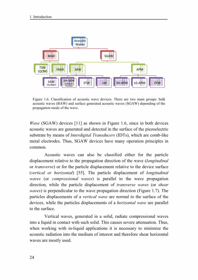
1. Introduction
24
Wave (SGAW) devices [11] as shown in Figure 1.6, since in both devices acoustic waves are generated and detected in the surface of the piezoelectric substrate by means of Interdigital Transducers (IDTs), which are comb-like metal electrodes. Thus, SGAW devices have many operation principles in common.
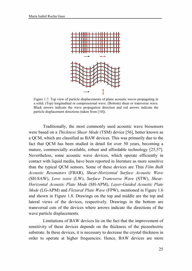
Acoustic waves can also be classified either for the particle displacement relative to the propagation direction of the wave (longitudinal or transverse) or for the particle displacement relative to the device surface (vertical or horizontal) [55]. The particle displacement of longitudinal
waves (or compressional waves) is parallel to the wave propagation direction, while the particle displacement of transverse waves (or shear
waves) is perpendicular to the wave propagation direction (Figure 1.7). The particles displacements of a vertical wave are normal to the surface of the devices, while the particles displacements of a horizontal wave are parallel to the surface.
Vertical waves, generated in a solid, radiate compressional waves into a liquid in contact with such solid. This causes severe attenuation. Thus, when working with in-liquid applications it is necessary to minimize the acoustic radiation into the medium of interest and therefore shear horizontal waves are mostly used.
Figure 1.6. Classification of acoustic wave devices. There are two main groups: bulk acoustic waves (BAW) and surface generated acoustic waves (SGAW) depending of the propagation mode of the wave.
AcousticWaves
BAW
TSM (QCM)
FBAR
SGAW
SAW
SAW (Rayleigh)
SH-SAW (Leaky orPseudo)
STW LW
APM
SH-APM LG-APM FPW
María Isabel Rocha Gaso
25
Traditionally, the most commonly used acoustic wave biosensors were based on a Thickness Shear Mode (TSM) device [56], better known as a QCM, which are classified as BAW devices. This was primarily due to the fact that QCM has been studied in detail for over 50 years, becoming a mature, commercially available, robust and affordable technology [25,57]. Nevertheless, some acoustic wave devices, which operate efficiently in contact with liquid media, have been reported in literature as more sensitive than the typical QCM sensors. Some of these devices are Thin Film Bulk
Acoustic Resonators (FBAR), Shear-Horizontal Surface Acoustic Wave (SH-SAW), Love wave (LW), Surface Transverse Wave (STW), Shear-
Horizontal Acoustic Plate Mode (SH-APM), Layer-Guided Acoustic Plate
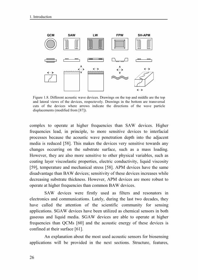
Mode (LG-APM) and Flexural Plate Wave (FPW), mentioned in Figure 1.6 and shown in Figure 1.8. Drawings on the top and middle are the top and lateral views of the devices, respectively. Drawings in the bottom are transversal cuts of the devices where arrows indicate the directions of the wave particle displacements.
Limitations of BAW devices lie on the fact that the improvement of sensitivity of these devices depends on the thickness of the piezoelectric substrate. In these devices, it is necessary to decrease the crystal thickness in order to operate at higher frequencies. Hence, BAW devices are more
Figure 1.7. Top view of particle displacements of plane acoustic waves propagating in a solid. (Top) longitudinal or compressional wave. (Bottom) shear or transverse wave. Black arrows indicate the wave propagation direction and red arrows indicate the particle displacement directions (taken from [10]).
1. Introduction
26
complex to operate at higher frequencies than SAW devices. Higher frequencies lead, in principle, to more sensitive devices to interfacial processes because the acoustic wave penetration depth into the adjacent media is reduced [58]. This makes the devices very sensitive towards any changes occurring on the substrate surface, such as a mass loading. However, they are also more sensitive to other physical variables, such as coating layer viscoelastic properties, electric conductivity, liquid viscosity [59], temperature and mechanical stress [58]. APM devices have the same disadvantage than BAW devices; sensitivity of these devices increases while decreasing substrate thickness. However, APM devices are more robust to operate at higher frequencies than common BAW devices.
SAW devices were firstly used as filters and resonators in electronics and communications. Lately, during the last two decades, they have called the attention of the scientific community for sensing applications. SGAW devices have been utilized as chemical sensors in both gaseous and liquid media. SGAW devices are able to operate at higher frequencies than QCMs [60] and the acoustic energy of these devices is confined at their surface [61].
An explanation about the most used acoustic sensors for biosensing applications will be provided in the next sections. Structure, features,
Figure 1.8. Different acoustic wave devices. Drawings on the top and middle are the top and lateral views of the devices, respectevely. Drawings in the bottom are transversal cuts of the devices where arrows indicate the directions of the wave particle displacements (modified from [87]).
QCM SAW LW
TopTop
E
SH-APMFPWQCM SAW LWQCM SAW LW
TopTop
E
SH-APMFPW
María Isabel Rocha Gaso
27
operation principle, operation frequencies, most common materials, sensitivities reported, advantages and disadvantages will be presented.
1.5.1 Quartz Crystal Microbalance (QCM)
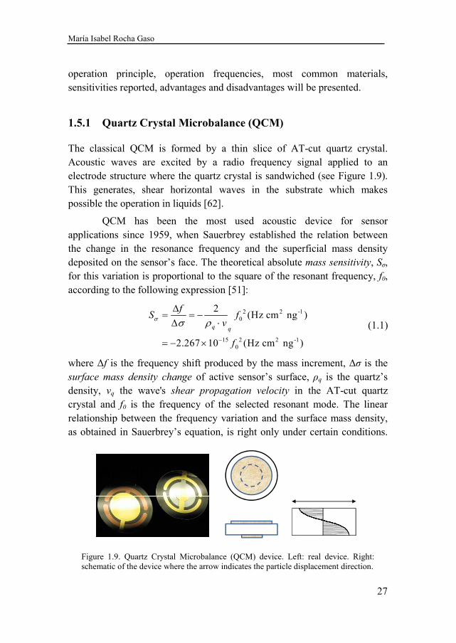
The classical QCM is formed by a thin slice of AT-cut quartz crystal. Acoustic waves are excited by a radio frequency signal applied to an electrode structure where the quartz crystal is sandwiched (see Figure 1.9). This generates, shear horizontal waves in the substrate which makes possible the operation in liquids [62].
QCM has been the most used acoustic device for sensor applications since 1959, when Sauerbrey established the relation between the change in the resonance frequency and the superficial mass density deposited on the sensor’s face. The theoretical absolute mass sensitivity, Sσ, for this variation is proportional to the square of the resonant frequency, f0, according to the following expression [51]:
2 2 -10
15 2 2 -10
2(Hz cm ng )
2.267 10 (Hz cm ng )
q q
fS f
v
f
σ σ ρ
−
∆= = −
∆ ⋅
= − ×
(1.1)
where ∆f is the frequency shift produced by the mass increment, ∆σ is the surface mass density change of active sensor’s surface, ρq is the quartz’s density, vq the wave's shear propagation velocity in the AT-cut quartz crystal and f0 is the frequency of the selected resonant mode. The linear relationship between the frequency variation and the surface mass density, as obtained in Sauerbrey’s equation, is right only under certain conditions.
Figure 1.9. Quartz Crystal Microbalance (QCM) device. Left: real device. Right: schematic of the device where the arrow indicates the particle displacement direction.
1. Introduction
28
Such equation is only valid when the layer deposited in the sensor’s face is very thin. In this condition, the material stays rigidly attached to the quartz surface, suffering a negligible deformation when the acoustic wave passes through it. A direct consequence of this is that the material’s elastic properties do not affect the sensor’s resonance frequency, and thus, the resonant frequency variations are exclusively due to a mass change effect. As the thickness of the deposited layer becomes thicker, this assumption is less valid. For thick deposited layers the resonator becomes sensitive to viscoelastic properties of the deposited layer’s material and Sauerbrey’s equation relation is not applicable.
As it can be observed in Equation (1.1), the theoretical mass sensitivity and, the sensitivity depends exclusively on the sensor’s intrinsic material properties and the resonance frequency. This makes the device ideal for sensing applications. Another figure of merit for sensors is the limit
of detection (LOD) or surface mass resolution (∆σr). Contrarily to the mass sensitivity, the LOD, not only depends on the sensor’s material properties, it also depends on the employed sensor’s characterization system. The characterization system limits the minimum signal that can be measured and distinguished from noise, i.e. ∆fmin is the minimum change in frequency that can be measured in an oscillator. Thus, for an AT-cut QCM the LOD can be obtained from Eq. (1.1), and is given by:
minLOD r
f
Sσ
σ∆
= ∆ = (1.2)
From the definition of the resonator quality factor (Q) [63,64], it can be followed that the minimum frequency shift detectable depends on the minimum detectable phase change on the frequency and the quality factor:
minmin 0
1
2f f
Q
ϕ∆∆ = (1.3)
Thus, from Eq. (1.2) and (1.3) it follows that the minimum detectable mass is given by:
min0
1LOD
2r fS Qσ
ϕσ
∆= ∆ =
⋅ (1.4)
Therefore, the minimum detectable mass attachment depends on the phase resolution ∆φmin, which depends on the respective readout circuit
María Isabel Rocha Gaso
29
used and on the signal-to-noise ratio that is required. In other words, one sensor can get different LODs depending on the characterization system. Moreover, Eq. (1.4) shows that for a given ∆φmin the surface mass resolution is relatively independent of the chosen resonance frequency, since typically the Q-factor is inversely proportional to the frequency and Sσ is directly proportional to the squared frequency (see Eq. (1.1)). Thus, increasing the frequency does not guarantee necessarily a higher surface mass resolution.
QCM technology is a well-established technique that has a huge field of applications in biochemistry and biotechnology. The availability for QCM to operate in liquid has extended the number of applications including the characterization of different type of molecular interactions and detection such as peptides [65], proteins [66], pesticides [9], oligonucleotides [67], bacteriophages [68], viruses [69], bacteria [70] and cells [71]; recently it has been applied for detection of DNA strands and genetically modified organisms (GMOs) [72]. Despite of the extensive use of QCM technology, some aspects such as the improvement of the sensitivity and the LOD are still desired in many applications. Absolute sensitivities of a 30 MHz QCM reach 66.6 cm2/g, with typical mass resolutions around 10 ng/cm2 [73]. Lower mass resolutions down to 1 ng/cm2 seem possible by improving the electronic characterization and read-out circuitry as well as the fluidic system.
Nowadays, in many applications an increase of sensitivity and decrease of LOD are desired. According to Sauerbrey’s equation, in order to increase the sensitivity, an increase in operating frequency is required. This leads to new problems that do not exist in low operation frequencies. In this sense, the main aspects to be solve when dealing with QCM sensors in high frequency conditions are the design of the characterization and read-out systems, the design and fabrication of the device, the sensor handling (as the high frequency device turns it very fragile [74]), the (micro)fluidic system, and costs. This is the reason why many commercial systems are already available in the market [43] for low frequencies around 10 MHz in fundamental mode or few tens of MHz in overtones, but not for fundamental mode frequencies around hundreds of MHz. Once all the issues related with the increase of frequency are solved, the next challenge would be the integration and their application in sensor arrays. In this sense, commercial QCM systems are mostly based on single element sensors, or on multi-
1. Introduction
30
channel systems composed of several single element sensors [75]. The integration shortcoming could be overcome with the apparition of FBAR.
1.5.2 Thin film bulk acoustic resonators (FBAR)
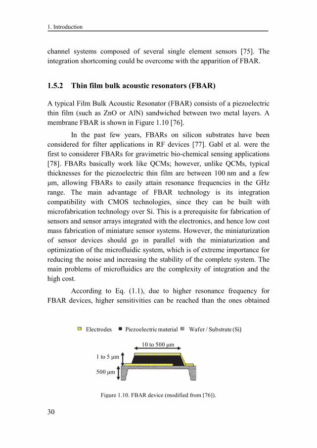
A typical Film Bulk Acoustic Resonator (FBAR) consists of a piezoelectric thin film (such as ZnO or AlN) sandwiched between two metal layers. A membrane FBAR is shown in Figure 1.10 [76].
In the past few years, FBARs on silicon substrates have been considered for filter applications in RF devices [77]. Gabl et al. were the first to considerer FBARs for gravimetric bio-chemical sensing applications [78]. FBARs basically work like QCMs; however, unlike QCMs, typical thicknesses for the piezoelectric thin film are between 100 nm and a few µm, allowing FBARs to easily attain resonance frequencies in the GHz range. The main advantage of FBAR technology is its integration compatibility with CMOS technologies, since they can be built with microfabrication technology over Si. This is a prerequisite for fabrication of sensors and sensor arrays integrated with the electronics, and hence low cost mass fabrication of miniature sensor systems. However, the miniaturization of sensor devices should go in parallel with the miniaturization and optimization of the microfluidic system, which is of extreme importance for reducing the noise and increasing the stability of the complete system. The main problems of microfluidics are the complexity of integration and the high cost.
According to Eq. (1.1), due to higher resonance frequency for FBAR devices, higher sensitivities can be reached than the ones obtained
Figure 1.10. FBAR device (modified from [76]).
Electrodes Piezoelectric material Wafer / Substrate (Si)
10 to 500 µm
1 to 5 µm
500 µm
María Isabel Rocha Gaso
31
with classical QCMs. Thin film electroacoustic technology has made possible to fabricate Quasi-Shear Mode Thin Film Bulk Acoustic Resonators
(S-FBAR), operating with a sufficient electromechanical coupling for use in liquid media at 1–2 GHz [79,80]. Weber et al. [81] also reported a S-FBAR resonator with ZnO C-axis 16° inclined relative to the surface normal and experimental biosensor sensitivity of 740.5 cm2/g and a minimum detectable mass of 2.3 ng/cm2 for a 790 MHz device. However, the higher frequency results in an increase of the noise of the read-out and characterization system; and the smaller size cause that the boundary conditions have a much stronger effect on the FBAR performance than on the QCM performance. This results in a higher mass sensitivity, but in an increased noise level as well, thus moderating the gain in mass resolution [82,83], as it was stated in the previous section. Hence, currently, only publications of network analyzer based FBAR sensor measurements have been published in the literature which show that the FBAR mass resolution is very similar if not slightly better than for oscillators based on conventional 10 MHz QCM sensors [81-84].
Over the last 5 years, some groups have proceeded with a number of experiments using and improving FBARs for biosensor applications, showing that FBAR could be a very promising technique. However, nowadays, FBAR technology requires a high research cost. Before dealing with this incoming technology, which mainly has the advantage of the miniaturization of the system, it is necessary to check some aspects, such as the increase of the noise when increasing the frequency, the dependence of the mass sensitivity with the electrode size, the optimization of the read out and characterization system for high frequency devices, etc. This can be done by using High Fundamental Frequency QCM (HFF-QCM) based on inverted MESA technology, thus avoiding all the drawbacks of FBAR technology (microfluidics, research cost, modeling, difficulty for achieving the generation of a pure shear mode excitation, etc.). When HFF-QCM technology shows that an increase in frequency leads to an increase in the mass resolution then, the next step will be to leap into FBAR technology to accomplish the integration of the system.
1. Introduction
32
1.5.3 Rayleigh wave (SAW)
Surface acoustic waves (SAW) are known since Lord Rayleigh proposed their existence in 1885. Rayleigh analyzed the propagation of elastic surface waves on isotropic media and stated that this kind of waves “played an
important part in earthquakes, and in the collision of elastic solids” [85]. These waves are modes of propagation along the free surface of an infinite half space in which the displacement amplitudes of the propagating waves decay in an exponential manner with depth beneath the surface. The associated energy density is concentrated within a distance of the order of a wavelength below the surface.
The first surface acoustic waves devices were possible thanks to the works of White and Voltmer in 1965 [86] where the IDTs were firstly reported for the generation of surface acoustic waves in a piezoelectric substrate.
The firsts SGAW devices operated with the Rayleigh wave which is a surface acoustic wave with longitudinal and transversal components. Thus, these first SGAW devices were called Surface Acoustic Wave (SAW) devices. Rayleigh waves have a substantial surface-normal (vertical) displacement with elliptical particle motion that easily dissipates the acoustic wave energy into the liquid, leading to excessive damping, and hence poor sensitivity and noise. Consequently, other types of SGAW devices, described later, were needed to work in liquid applications.
The input port of a SGAW sensor -comprised of metal electrodes (IDTs) deposited or photodesigned on an optically polished surface of a piezoelectric crystal- launches a mechanical acoustic wave into the piezoelectric material due to the application of a sinusoidal input voltage (radio frequency signal), Vin, and to the inverse piezoelectric phenomenon. The acoustic wave propagates through the substrate until it reaches the output IDT were the wave is converted back to an electric signal, Vout, thanks to the direct piezoelectric phenomenon (Figure 1.11). Physical interactions at the sensor surface cause changes in the acoustic wave propagation velocity and amplitude. These changes are translated in changes in the amplitude and phase relations between Vin and Vout, which can be measured with network analyzers and vector voltmeters. On the other hand, these wave's propagation velocity changes can be translated to a change in
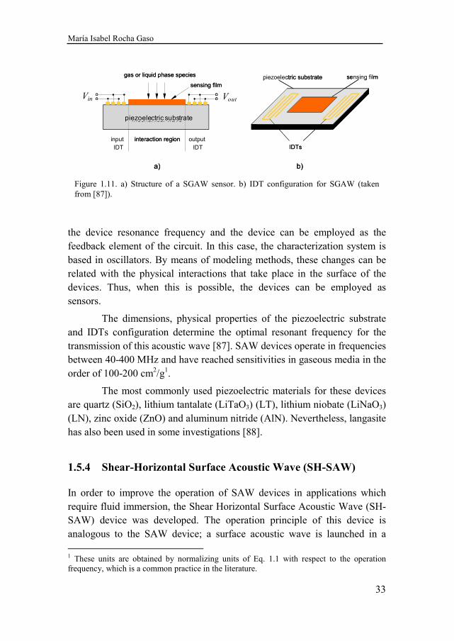
María Isabel Rocha Gaso
33
the device resonance frequency and the device can be employed as the feedback element of the circuit. In this case, the characterization system is based in oscillators. By means of modeling methods, these changes can be related with the physical interactions that take place in the surface of the devices. Thus, when this is possible, the devices can be employed as sensors.
The dimensions, physical properties of the piezoelectric substrate and IDTs configuration determine the optimal resonant frequency for the transmission of this acoustic wave [87]. SAW devices operate in frequencies between 40-400 MHz and have reached sensitivities in gaseous media in the order of 100-200 cm2/g1.
The most commonly used piezoelectric materials for these devices are quartz (SiO2), lithium tantalate (LiTaO3) (LT), lithium niobate (LiNaO3) (LN), zinc oxide (ZnO) and aluminum nitride (AlN). Nevertheless, langasite has also been used in some investigations [88].
1.5.4 Shear-Horizontal Surface Acoustic Wave (SH-SAW)
In order to improve the operation of SAW devices in applications which require fluid immersion, the Shear Horizontal Surface Acoustic Wave (SH-SAW) device was developed. The operation principle of this device is analogous to the SAW device; a surface acoustic wave is launched in a 1 These units are obtained by normalizing units of Eq. 1.1 with respect to the operation frequency, which is a common practice in the literature.
Figure 1.11. a) Structure of a SGAW sensor. b) IDT configuration for SGAW (taken from [87]).
gas or liquid phase species
sensing film
mechanical wave
interaction regioninput output
IDT IDT
Vi Vo
piezoelectric substrate sensing film
IDTs
a) b)
gas or liquid phase species
sensing film
mechanical wave
interaction regioninput output
IDT IDT
Vi Vo
piezoelectric substrate sensing film
IDTs
a) b)
piezoelectric substrate
Vin Vout
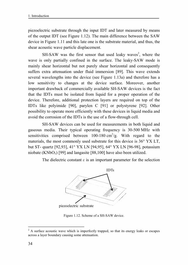
1. Introduction
34
piezoelectric substrate through the input IDT and later measured by means of the output IDT (see Figure 1.12). The main difference between the SAW device in Figure 1.11 and this late one is the substrate material, and thus, the shear acoustic wave particle displacement.
SH-SAW was the first sensor that used leaky waves2, where the wave is only partially confined in the surface. The leaky-SAW mode is mainly shear horizontal but not purely shear horizontal and consequently suffers extra attenuation under fluid immersion [89]. This wave extends several wavelengths into the device (see Figure 1.13a) and therefore has a low sensitivity to changes at the device surface. Moreover, another important drawback of commercially available SH-SAW devices is the fact that the IDTs must be isolated from liquid for a proper operation of the device. Therefore, additional protection layers are required on top of the IDTs like polyimide [90], parylen C [91] or polystyrene [92]. Other possibility to operate more efficiently with these devices in liquid media and avoid the corrosion of the IDTs is the use of a flow-through cell.
SH-SAW devices can be used for measurements in both liquid and gaseous media. Their typical operating frequency is 30-500 MHz with sensitivities comprised between 100-180 cm2/g. With regard to the materials, the most commonly used substrate for this device is 36° YX LT, but ST- quartz [92,93], 41° YX LN [94,95], 64° YX LN [96-98], potassium niobate (KNbO3) [99] and langasite [88,100] have also been utilized.
The dielectric constant ε is an important parameter for the selection
2 A surface acoustic wave which is imperfectly trapped, so that its energy leaks or escapes across a layer boundary causing some attenuation.
Figure 1.12. Scheme of a SH-SAW device.
piezoelectric substrate
IDTs
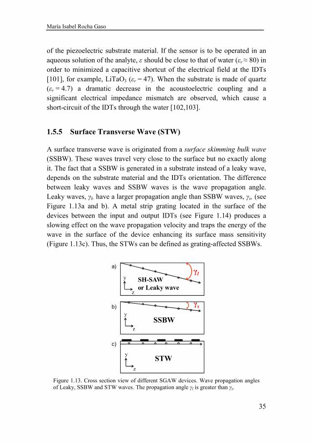
María Isabel Rocha Gaso
35
of the piezoelectric substrate material. If the sensor is to be operated in an aqueous solution of the analyte, ε should be close to that of water (εr ≈ 80) in order to minimized a capacitive shortcut of the electrical field at the IDTs [101], for example, LiTaO3 (εr = 47). When the substrate is made of quartz (εr = 4.7) a dramatic decrease in the acoustoelectric coupling and a significant electrical impedance mismatch are observed, which cause a short-circuit of the IDTs through the water [102,103].
1.5.5 Surface Transverse Wave (STW)
A surface transverse wave is originated from a surface skimming bulk wave (SSBW). These waves travel very close to the surface but no exactly along it. The fact that a SSBW is generated in a substrate instead of a leaky wave, depends on the substrate material and the IDTs orientation. The difference between leaky waves and SSBW waves is the wave propagation angle. Leaky waves, γl, have a larger propagation angle than SSBW waves, γs, (see Figure 1.13a and b). A metal strip grating located in the surface of the devices between the input and output IDTs (see Figure 1.14) produces a slowing effect on the wave propagation velocity and traps the energy of the wave in the surface of the device enhancing its surface mass sensitivity (Figure 1.13c). Thus, the STWs can be defined as grating-affected SSBWs.
Figure 1.13. Cross section view of different SGAW devices. Wave propagation angles of Leaky, SSBW and STW waves. The propagation angle γl is greater than γs.
SH-SAW
or Leaky wave
γl
γs
SSBW
STW
a)
b)
c)
y
z
y
z
y
z
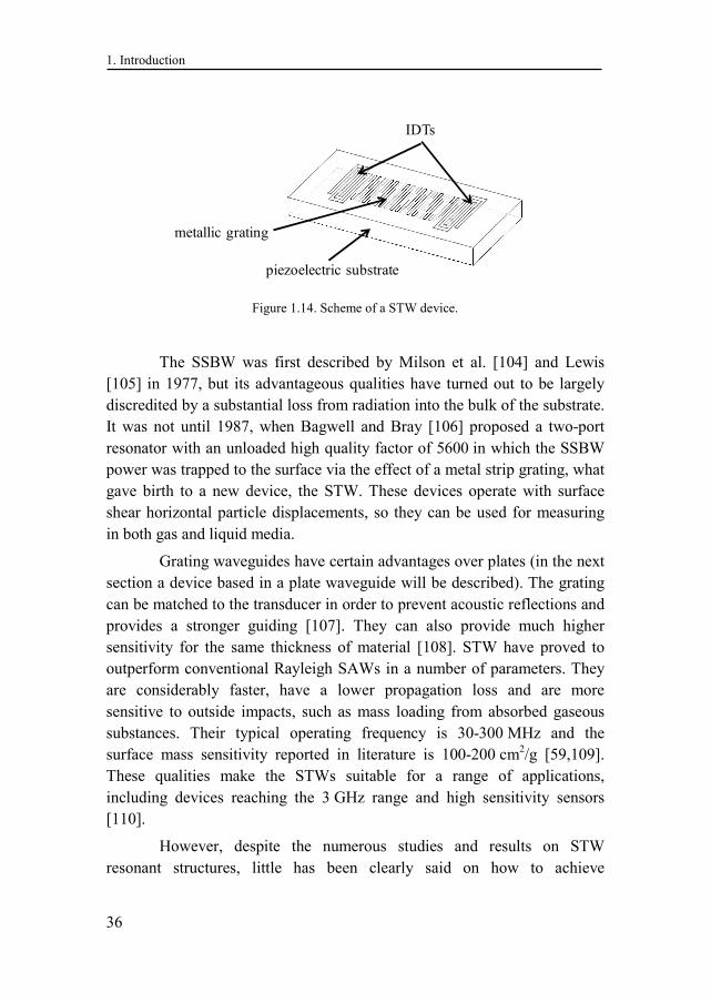
1. Introduction
36
The SSBW was first described by Milson et al. [104] and Lewis [105] in 1977, but its advantageous qualities have turned out to be largely discredited by a substantial loss from radiation into the bulk of the substrate. It was not until 1987, when Bagwell and Bray [106] proposed a two-port resonator with an unloaded high quality factor of 5600 in which the SSBW power was trapped to the surface via the effect of a metal strip grating, what gave birth to a new device, the STW. These devices operate with surface shear horizontal particle displacements, so they can be used for measuring in both gas and liquid media.
Grating waveguides have certain advantages over plates (in the next section a device based in a plate waveguide will be described). The grating can be matched to the transducer in order to prevent acoustic reflections and provides a stronger guiding [107]. They can also provide much higher sensitivity for the same thickness of material [108]. STW have proved to outperform conventional Rayleigh SAWs in a number of parameters. They are considerably faster, have a lower propagation loss and are more sensitive to outside impacts, such as mass loading from absorbed gaseous substances. Their typical operating frequency is 30-300 MHz and the surface mass sensitivity reported in literature is 100-200 cm2/g [59,109]. These qualities make the STWs suitable for a range of applications, including devices reaching the 3 GHz range and high sensitivity sensors [110].
However, despite the numerous studies and results on STW resonant structures, little has been clearly said on how to achieve
Figure 1.14. Scheme of a STW device.
piezoelectric substrate
IDTs
metallic grating
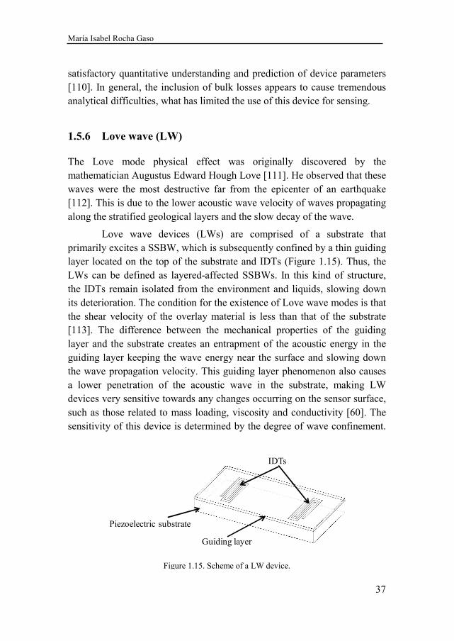
María Isabel Rocha Gaso
37
satisfactory quantitative understanding and prediction of device parameters [110]. In general, the inclusion of bulk losses appears to cause tremendous analytical difficulties, what has limited the use of this device for sensing.
1.5.6 Love wave (LW)
The Love mode physical effect was originally discovered by the mathematician Augustus Edward Hough Love [111]. He observed that these waves were the most destructive far from the epicenter of an earthquake [112]. This is due to the lower acoustic wave velocity of waves propagating along the stratified geological layers and the slow decay of the wave.
Love wave devices (LWs) are comprised of a substrate that primarily excites a SSBW, which is subsequently confined by a thin guiding layer located on the top of the substrate and IDTs (Figure 1.15). Thus, the LWs can be defined as layered-affected SSBWs. In this kind of structure, the IDTs remain isolated from the environment and liquids, slowing down its deterioration. The condition for the existence of Love wave modes is that the shear velocity of the overlay material is less than that of the substrate [113]. The difference between the mechanical properties of the guiding layer and the substrate creates an entrapment of the acoustic energy in the guiding layer keeping the wave energy near the surface and slowing down the wave propagation velocity. This guiding layer phenomenon also causes a lower penetration of the acoustic wave in the substrate, making LW devices very sensitive towards any changes occurring on the sensor surface, such as those related to mass loading, viscosity and conductivity [60]. The sensitivity of this device is determined by the degree of wave confinement.
Figure 1.15. Scheme of a LW device.
Piezoelectric substrate
IDTs
Guiding layer
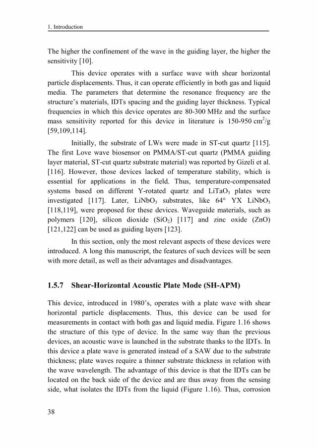
1. Introduction
38
The higher the confinement of the wave in the guiding layer, the higher the sensitivity [10].
This device operates with a surface wave with shear horizontal particle displacements. Thus, it can operate efficiently in both gas and liquid media. The parameters that determine the resonance frequency are the structure’s materials, IDTs spacing and the guiding layer thickness. Typical frequencies in which this device operates are 80-300 MHz and the surface mass sensitivity reported for this device in literature is 150-950 cm2/g [59,109,114].
Initially, the substrate of LWs were made in ST-cut quartz [115]. The first Love wave biosensor on PMMA/ST-cut quartz (PMMA guiding layer material, ST-cut quartz substrate material) was reported by Gizeli et al. [116]. However, those devices lacked of temperature stability, which is essential for applications in the field. Thus, temperature-compensated systems based on different Y-rotated quartz and LiTaO3 plates were investigated [117]. Later, LiNbO3 substrates, like 64° YX LiNbO3
[118,119], were proposed for these devices. Waveguide materials, such as polymers [120], silicon dioxide (SiO2) [117] and zinc oxide (ZnO) [121,122] can be used as guiding layers [123].
In this section, only the most relevant aspects of these devices were introduced. A long this manuscript, the features of such devices will be seen with more detail, as well as their advantages and disadvantages.
1.5.7 Shear-Horizontal Acoustic Plate Mode (SH-APM)
This device, introduced in 1980’s, operates with a plate wave with shear horizontal particle displacements. Thus, this device can be used for measurements in contact with both gas and liquid media. Figure 1.16 shows the structure of this type of device. In the same way than the previous devices, an acoustic wave is launched in the substrate thanks to the IDTs. In this device a plate wave is generated instead of a SAW due to the substrate thickness; plate waves require a thinner substrate thickness in relation with the wave wavelength. The advantage of this device is that the IDTs can be located on the back side of the device and are thus away from the sensing side, what isolates the IDTs from the liquid (Figure 1.16). Thus, corrosion
María Isabel Rocha Gaso
39
problems on electrodes resulting in deterioration of the sensor response are avoided. The most commonly used substrates for this device are ST-cut quartz and ZX LiNbO3.
The parameters that determine the resonance frequency of this device are the materials and thickness of the substrate and spacing of IDTs. The typical operating frequency of this device is between 25-200 MHz and the surface mass sensitivity reported in literature is 20-50 cm2/g [59,109,124]. Theoretically, the sensitivity of this device for an isotropic plate is given by Sσ = −J/ρ·d; where J = 1/2 for the mode n = 0 and J = 1 for higher plate modes (n > 0), ρ is the plate density and d is the plate thickness [59]. Decreasing the plate thickness increases the frequencies of higher plate modes of the SH-APM device and it also increases mass sensitivity. Thus, higher-order modes appeared to be more sensitive than lower-order modes, although they have more transmission losses [125].
The SH-APMs have been used for measuring mass change in liquid media and also for detecting biological molecules [126]. However, the use of APM delay lines has been hampered by the relative immaturity of the associated design techniques. The principle issue in the design of APM delay lines is to excite and detect electrically a single acoustic mode within the plate with low distortion from intermode interference or multiple waveguide reflections. In practice, several acoustic plate modes are usually excited simultaneously, but the frequency separation between these modes is often limited; this can produce a hopping mode in an oscillator circuit [60]. This is the reason why SH-APMs are difficult to operate in a standard oscillator circuit, which is one of the main drawbacks of this device.
Figure 1.16. Structure of an SH-APM sensor (taken from [87]).
viscous conductiveliquid medium
input
IDT
output
IDT
viscous conductiveliquid medium
input
IDT
output
IDT
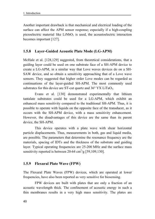
1. Introduction
40
Another important drawback is that mechanical and electrical loading of the surface can affect the APM sensor response; especially if a high-coupling piezoelectric material like LiNbO3 is used, the acoustoelectric interaction becomes important [127].
1.5.8 Layer-Guided Acoustic Plate Mode (LG-APM)
McHale et al. [128,129] suggested, from theoretical considerations, that a guiding layer could be used on one substrate face of a SH-APM device to create a LG-APM, in a similar way that Love waves devices do on a SH-SAW device, and so obtain a sensitivity approaching that of a Love wave sensors. They suggested that higher order Love modes can be regarded as continuations of the layer-guided SH-APM. The most commonly used substrates for this device are ST-cut quartz and 36° YX LiTaO3.
Evans et al. [130] demonstrated experimentally that lithium tantalate substrates could be used for a LG-APM, which exhibit an enhanced mass sensitivity compared to the traditional SH-APM. Thus, it is possible to operate with liquids on the opposite face of the transducer, as it occurs with the SH-APM device, with a mass sensitivity enhancement. However, the disadvantages of this device are the same than its parent device, the SH-APM.
This device operates with a plate wave with shear horizontal particle displacements. Thus, measurements in both, gas and liquid media, are possible. The parameters that determine the resonance frequency are the materials, spacing of IDTs and the thickness of the substrate and guiding layer. Typical operating frequencies are 25-200 MHz and the surface mass sensitivity reported is between 20-64 cm2/g [59,109,130].
1.5.9 Flexural Plate Wave (FPW)
The Flexural Plate Waves (FPW) devices, which are operated at lower frequencies, have also been reported as very sensitive for biosensing.
FPW devices are built with plates that are only a fraction of an acoustic wavelength thick. The confinement of acoustic energy in such a thin membranes results in a very high mass sensitivity. The plates are
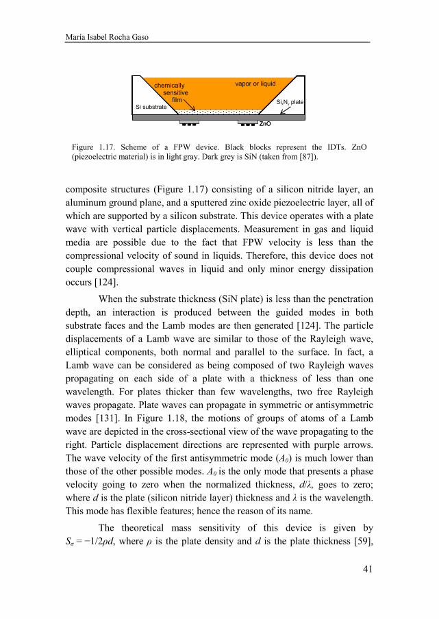
María Isabel Rocha Gaso
41
composite structures (Figure 1.17) consisting of a silicon nitride layer, an aluminum ground plane, and a sputtered zinc oxide piezoelectric layer, all of which are supported by a silicon substrate. This device operates with a plate wave with vertical particle displacements. Measurement in gas and liquid media are possible due to the fact that FPW velocity is less than the compressional velocity of sound in liquids. Therefore, this device does not couple compressional waves in liquid and only minor energy dissipation occurs [124].
When the substrate thickness (SiN plate) is less than the penetration depth, an interaction is produced between the guided modes in both substrate faces and the Lamb modes are then generated [124]. The particle displacements of a Lamb wave are similar to those of the Rayleigh wave, elliptical components, both normal and parallel to the surface. In fact, a Lamb wave can be considered as being composed of two Rayleigh waves propagating on each side of a plate with a thickness of less than one wavelength. For plates thicker than few wavelengths, two free Rayleigh waves propagate. Plate waves can propagate in symmetric or antisymmetric modes [131]. In Figure 1.18, the motions of groups of atoms of a Lamb wave are depicted in the cross-sectional view of the wave propagating to the right. Particle displacement directions are represented with purple arrows. The wave velocity of the first antisymmetric mode (A0) is much lower than those of the other possible modes. A0 is the only mode that presents a phase velocity going to zero when the normalized thickness, d/λ, goes to zero; where d is the plate (silicon nitride layer) thickness and λ is the wavelength. This mode has flexible features; hence the reason of its name.
The theoretical mass sensitivity of this device is given by Sσ = −1/2ρd, where ρ is the plate density and d is the plate thickness [59],
Figure 1.17. Scheme of a FPW device. Black blocks represent the IDTs. ZnO (piezoelectric material) is in light gray. Dark grey is SiN (taken from [87]).
vapor or liquid
Si substrateSixNy plate
ZnO
chemicallysensitive
film
vapor or liquid
Si substrateSixNy plate
ZnO
chemicallysensitive
film
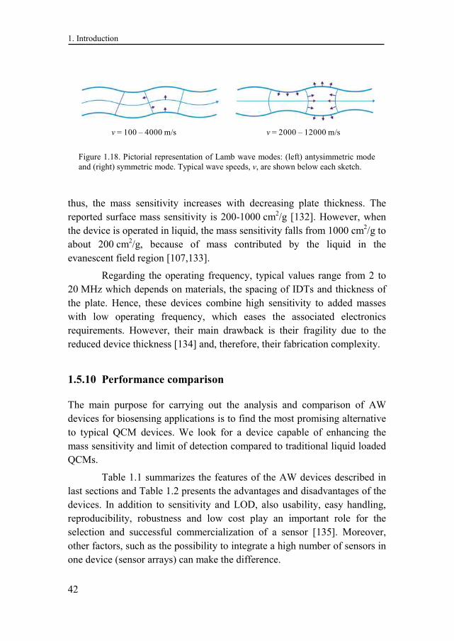
1. Introduction
42
thus, the mass sensitivity increases with decreasing plate thickness. The reported surface mass sensitivity is 200-1000 cm2/g [132]. However, when the device is operated in liquid, the mass sensitivity falls from 1000 cm2/g to about 200 cm2/g, because of mass contributed by the liquid in the evanescent field region [107,133].
Regarding the operating frequency, typical values range from 2 to 20 MHz which depends on materials, the spacing of IDTs and thickness of the plate. Hence, these devices combine high sensitivity to added masses with low operating frequency, which eases the associated electronics requirements. However, their main drawback is their fragility due to the reduced device thickness [134] and, therefore, their fabrication complexity.
1.5.10 Performance comparison
The main purpose for carrying out the analysis and comparison of AW devices for biosensing applications is to find the most promising alternative to typical QCM devices. We look for a device capable of enhancing the mass sensitivity and limit of detection compared to traditional liquid loaded QCMs.
Table 1.1 summarizes the features of the AW devices described in last sections and Table 1.2 presents the advantages and disadvantages of the devices. In addition to sensitivity and LOD, also usability, easy handling, reproducibility, robustness and low cost play an important role for the selection and successful commercialization of a sensor [135]. Moreover, other factors, such as the possibility to integrate a high number of sensors in one device (sensor arrays) can make the difference.
Figure 1.18. Pictorial representation of Lamb wave modes: (left) antysimmetric mode and (right) symmetric mode. Typical wave speeds, v, are shown below each sketch.
v = 100 – 4000 m/s v = 2000 – 12000 m/s
María Isabel Rocha Gaso
43
Traditional QCMs have lower mass sensitivity than the SAW devices mentioned in this manuscript. In principle, the sensitivity of these devices could be improved by increasing the operating frequency. Nevertheless, higher fundamental frequencies lead to more fragile QCM devices.
FBARs have a great mass sensitivity and they offer a great opportunity for miniaturization and CMOS compatibility. However, the main drawbacks of these sensors are their high fabrication complexity, which requires a high research cost for starting to work with them, and their high operating frequency, which poses a great challenge for the electronic characterization system.
SAW (Rayleigh waves) do not operate efficiently in liquids, so they are discarded for the purpose of this Thesis. On the other hand, STW and LW devices can be considered as an improved version of SH-SAW, since, as explained before, in those devices the acoustic wave energy is better confined in the surface of the device. Additionally, LW devices are more physically robust than QCMs and allow multi-arrays sensor configurations.
SH-APMs do not improve significantly the mass sensitivity of QCMs, so there is no sense in working with these devices when the purpose is to change the sensor technology for improving considerably the mass sensitivity and LOD of QCMs. Furthermore, these devices are difficult to operate with a single mode.
Since LG-APMs are derived from SH-APMs they are also difficult to operate with a single mode. Moreover, the reported mass sensitivity does not improve greatly the mass sensitivity of QCMs.
Finally, FPW have a great mass sensitivity and works at lower frequencies, which is a great advantage. However, this mass sensitivity greatly decreases when working in liquids and these devices are complex to fabricate.
Among SGAW devices, researchers seem to be more attracted to LW devices due to its features. LW sensors are the most sensitive SGAW when working with liquids. The experimental results obtained with LW sensors also point them as the most promising device for this purpose (see next section). It is clear that the commercial trend has been directed towards the
1. Introduction
44
use of LW for a more stable and efficient biosensor system, while other SGAW devices setups have not get past the laboratory or the patent stages.
A robust sensor system based on LW sensors would be extremely competitive to existing commercially available biosensing technologies. However, LW devices still have some hurdles [39] and challenges [11,135] to clear for its application as biosensors. They are sensitive to changes in the viscoelastic properties of the coating, which complicates the results interpretation. LW devices fabrication process is more complex than for QCMs and the materials involved for LW devices fabrication are still under investigation. In addition, much research and efforts are still required addressing the fluidic of LW devices for biosensors, since the device response is altered by the flow-through cell.
Next, the state-of-the art of LW biosensors, which point them as very promising tools in the field, is given, as well as their trends and challenges.
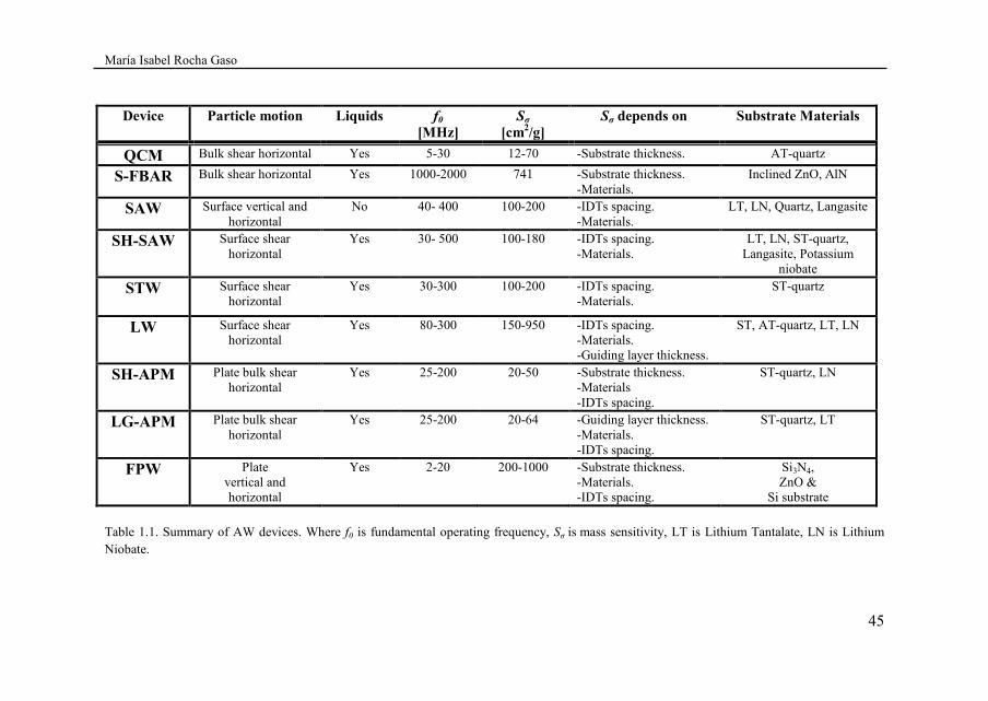
María Isabel Rocha Gaso
45
Device Particle motion Liquids f0 [MHz]
Sσ
[cm2/g] Sσ depends on Substrate Materials
QCM Bulk shear horizontal Yes 5-30 12-70 -Substrate thickness. AT-quartz
S-FBAR Bulk shear horizontal Yes 1000-2000 741 -Substrate thickness. -Materials.
Inclined ZnO, AlN
SAW Surface vertical and horizontal
No 40- 400 100-200 -IDTs spacing. -Materials.
LT, LN, Quartz, Langasite
SH-SAW Surface shear horizontal
Yes 30- 500 100-180 -IDTs spacing. -Materials.
LT, LN, ST-quartz, Langasite, Potassium
niobate
STW
Surface shear horizontal
Yes 30-300 100-200 -IDTs spacing. -Materials.
ST-quartz
LW Surface shear horizontal
Yes 80-300 150-950 -IDTs spacing. -Materials. -Guiding layer thickness.
ST, AT-quartz, LT, LN
SH-APM Plate bulk shear horizontal
Yes 25-200 20-50 -Substrate thickness. -Materials -IDTs spacing.
ST-quartz, LN
LG-APM Plate bulk shear horizontal
Yes 25-200 20-64 -Guiding layer thickness. -Materials. -IDTs spacing.
ST-quartz, LT
FPW Plate vertical and horizontal
Yes 2-20 200-1000 -Substrate thickness. -Materials. -IDTs spacing.
Si3N4, ZnO &
Si substrate
Table 1.1. Summary of AW devices. Where f0 is fundamental operating frequency, Sσ is mass sensitivity, LT is Lithium Tantalate, LN is Lithium Niobate.
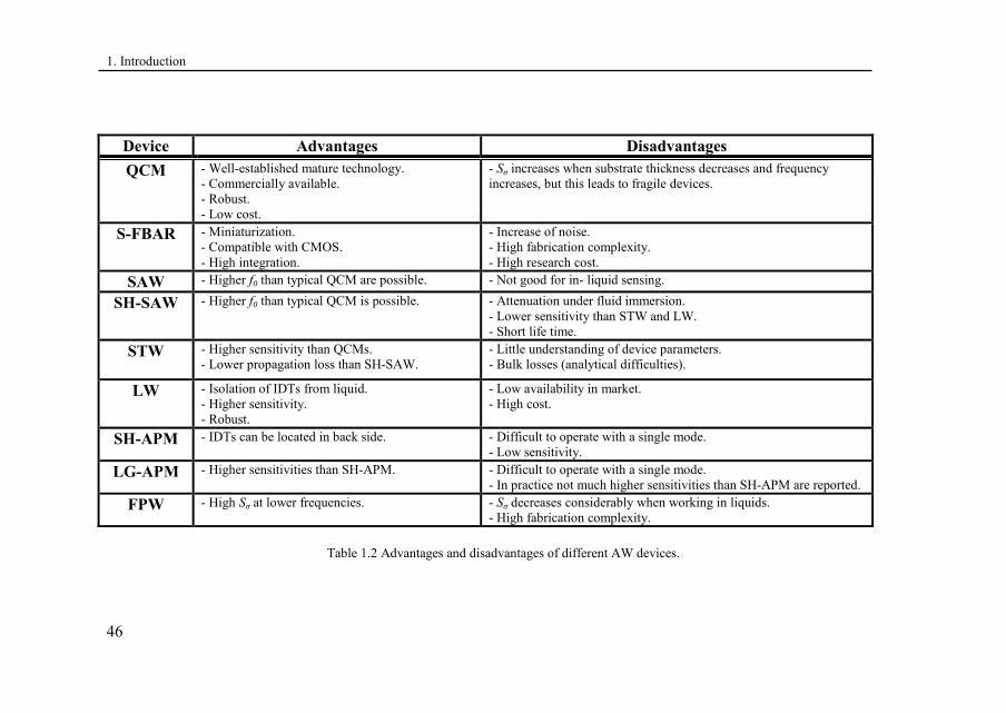
1. Introduction
46
Device Advantages Disadvantages
QCM - Well-established mature technology. - Commercially available. - Robust. - Low cost.
- Sσ increases when substrate thickness decreases and frequency increases, but this leads to fragile devices.
S-FBAR - Miniaturization. - Compatible with CMOS. - High integration.
- Increase of noise. - High fabrication complexity. - High research cost.
SAW - Higher f0 than typical QCM are possible. - Not good for in- liquid sensing.
SH-SAW - Higher f0 than typical QCM is possible. - Attenuation under fluid immersion. - Lower sensitivity than STW and LW. - Short life time.
STW
- Higher sensitivity than QCMs. - Lower propagation loss than SH-SAW.
- Little understanding of device parameters. - Bulk losses (analytical difficulties).
LW - Isolation of IDTs from liquid. - Higher sensitivity. - Robust.
- Low availability in market. - High cost.
SH-APM - IDTs can be located in back side. - Difficult to operate with a single mode. - Low sensitivity.
LG-APM - Higher sensitivities than SH-APM. - Difficult to operate with a single mode. - In practice not much higher sensitivities than SH-APM are reported.
FPW - High Sσ at lower frequencies.
- Sσ decreases considerably when working in liquids. - High fabrication complexity.
Table 1.2 Advantages and disadvantages of different AW devices.

María Isabel Rocha Gaso
47
1.6 LW biosensors state-of-the-art
The first approaches employing LW for biochemical sensing were reported in 1992 by Kovacs et al. [136] and by Gizeli et al. [116], who first demonstrated the use of such devices as mass sensing biosensors in liquids. However, it was not until 1997 that LW acoustic devices were used to detect real-time antigen-antibody interactions in liquid media [137].
In 1999, a contactless LW device was built in order to protect electrodes from the conductive and chemically aggressive liquids used in biosensing [138]. The advantage of this technique is that no wire bonding is required. However, the authors state that further efforts are needed to reduce the insertion loss of the device, miniaturize the required microwave set-up and increase its sensitivity.
In 2000, a dual channel LW device was used as a biosensor to simultaneously detect Legionella and E. coli by Howe and Harding [139]. In this approach, a novel protocol for coating bacteria on the sensor surface prior to addition of the antibody was introduced. Quantitative results were obtained for both species down to 106 cells/mL, within 3 h.
In 2003, a LW immunosensor was designed as a model for virus or bacteria detection in liquids (drinking or bathing water, food, etc.) by Tamarin et al. [140]. They grafted a monoclonal antibody (AM13 MAb) against M13 bacteriophage on the device surface (SiO2) and sensed the M13 bacteriophage/AM13 immunoreaction. The authors remarked the potentialities of such acoustic biosensors for biological detection. The same year, it was shown that mass sensitivity of LW devices with ZnO guiding layer was larger than that of sensors with SiO2 guiding layers [114]. The authors of this work monitored adsorption of rat immunoglobulin G, obtaining mass sensitivities as high as 950 cm2/g. They pointed out that such a device was a promising candidate for immunosensing applications.
An aptamer-based LW sensor which allowed the detection of small molecules was developed by Schlensog et al. in 2004 [141]. This biosensor offers an advantage over immunosensors, since it does not require the production of antibodies against toxic substances. A LW biosensor for the detection of pathogenic spores at or below inhalational infectious levels was
1. Introduction
48
reported by Branch et al. in 2004 [142]. A monoclonal antibody with a high degree of selectivity for anthrax spores was used to capture the non-pathogenic simulant Bacillus thuringiensis B8 spores in aqueous conditions. The authors stated that acoustic LW biosensors will have widespread application for whole-cell pathogen detection.
Moll et al. developed an innovative method for the detection of E.
coli employing an LW device in 2007 [143]; it consisted of grafting goat anti-mouse antibodies (GAM) onto the sensor surface and introducing E.
coli bacteria mixed with anti-E. coli MAb in a second step. The sensor response time was shorter when working at 37ºC, providing results in less than 1 hour with a detection threshold of 106 bacteria/mL. More recently, the same group described a multipurpose LW immunosensor for the detection of bacteria, virus and proteins [144]. They detected bacteriophages and proteins with a LOD of 1 µg/mL for protein and 106 cells/mL for bacteria, with good specificity and reproducibility. The authors stated that whole bacteria could be detected in less than one hour.
Andrä et al. used a LW sensor to investigate the mode of action and the lipid specificity of human antimicrobial peptides [145]. They analyzed the interaction of those peptides with model membranes. These membranes, when attached to the sensor surface, mimic the cytoplasmic and the outer bacterial membrane.
A LW immunosensor was used in 2008 by Bisoffi et al. [146] to detect Coxsackie virus B4 and Sin Nombre Virus (SNV), a member of the hantavirus family. They described a robust biosensor that combines the sensitivity of LW-SAW at a frequency of 325 MHz with the specificity provided by monoclonal and recombinant antibodies for the detection of viral agents. Rapid detection (within seconds) for increasing virus concentrations was reported. The biosensor was able to detect SNV at doses lower than the load of virus typically found in a human patient suffering from hantavirus cardiopulmonary syndrome.
In 2009, it was shown the possibility to graft streptavidin-gold molecules onto a LW sensor surface in a controlled way and was demonstrated the capability of the sensor to detect nano-particles in aqueous media by Fissi et al. [147]. In 2010, a complementary metal–oxide semiconductor CMOS-LW biosensor for breast cancer biomarker detection
María Isabel Rocha Gaso
49
was presented by Tigli et al. [148]. This biosensor was fabricated using CMOS technology and used gold as the guiding layer and as the interface material between the biological sensing medium and the transducer.
LW devices were used as sensors for okadaic acid immono-detection through immobilized specific antibodies by Fournel et al. [149]. They obtained three times higher frequency shifts with the okadaic acid than with an irrelevant peptide control line.
A LW based bacterial biosensor for the detection of heavy metal in liquid media was reported in 2011 by Gammoudi et al. [150]. Whole bacteria (E. coli) were fixed as bioreceptors onto the acoustic path of the sensor coated with a polyelectrolyte multilayer using a layer by layer electrostatic self-assembly procedure. Changes of bacteria's viscoelastic equivalent parameters in presence of toxic heavy metals were monitored. Also in 2011, Oh et al. developed a Love wave biosensor for multi-bioanalyte simultaneous detections in 2011 [151].
A LW-based wireless biosensor for the simultaneous detection of two different concentrations of anti-dinitrophenyl-KLH (anti-DNP) rabbit immunoglobulin G (IgG) in a single sensor was presented by Song et al. in 2011 [152]. They used poly(methyl-methacrylate) (PMMA) guiding layer and two sensitive films (Cr/Au). A LW sensor whose phase-shifts as a function of the immobilized antibody quantity, combined with an active acoustic mixing device, was proposed by Kardous et al. [1] in 2011. They assessed that mixing at the droplet level increases antibodies transfer to a sensing area surface and increases the reaction kinetics by removing the dependency with the protein diffusion coefficient in a liquid, while inducing minimum disturbance to the sensing capability of the Love mode.
In 2012, Matatagui et al. developed a Love-wave immunosensor with a PDMS microfluidic chip which detected the phage M13 through the mouse monoclonal antibody anti-M13 [153].
Saitakis et al. stated in 2012 that LW sensors can detect cells mostly via their sensitivity in viscoelasticity and mechanical properties and that these sensors are sensitive to the basal membrane of the cells and the adhesion proteins on the surface. They remarked, that Love-wave sensor also can directly measure cell/substrate bonds via acoustic damping and provide 2D kinetic and affinity parameters [154].
1. Introduction
50
Also in 2012, Mitsakakis et al. carried out multi-sample measurements using a LW sensor. They successfully detected specific interaction between patterned lipids’ head groups with target analytes [155].
A wireless LW-based biosensing platform was developed for the detection of protein binding by Cheng et al. [156] in 2012. The platform consisted of a microfluidic flow-cell, the wireless LW device, a syringe pump and a network analyzer connected to a personal computer.
LW sensors have been also used to study the properties of protein layers [157], DNA [158,159] and detect the adsorption and desorption of lipid layers [160].
Currently, the only commercial LW biosensor system available in the market, sam® 5, is commercialized by the German company SAW
Instruments GmbH. Broker et al. fabricated a nanostructured chip surface which enabled binding via spaced antibodies specifically targeting surface proteins of cancer cells and detection of extremely low numbers of circulating tumor cells (CTC) without labeling using this biosensing system [161]. Senseor company (Mougins, France) also has a commercially available microbalance development kit (SAW-MDK1) which consists of a two-channel LW delay lines.
1.7 Trends and challenges of LW biosensors
LW biosensors have not been very well recognized by the scientific community [61] nor by the market yet. This might be due to the technological hindrances found for applying this device as a biosensor. LW devices are sensitive to changes in the viscoelastic properties of the coating, which complicates the results interpretation. The combination with other detection methods, such as optical [11,53], chromatographic [162] or even a different acoustic technology like QCM could help to the parameter extraction and therefore to the results interpretation. In this sense, reports about applications where mass alterations are separated from viscoelastic effects can enhance the acceptance of LW sensors [61].
Another aspect which has limited the use of LW technology in biosensors is the sensor package, necessary for in-liquid applications. LW biosensors packaging needs further development and cost reduction. The
María Isabel Rocha Gaso
51
packages cost ten times more than the sensors they contain [108]. Moreover, a suitable design most be conceived in order to minimize the perturbation of the sensor response. In addition, much research and efforts are still required addressing the fluidic technology issue. Integration and automation with the electronic characterization system and flow cells reduce costs of the system and increase the throughput.
Mathematical modeling and simulations of these devices are also essential for the development of new sensor structures, especially with respect to the study of new materials, dimensions and wave propagation [61]. Numerical calculations and FEM analysis of LW sensors could help for further understanding of these devices. For instance, the simulations can predict an increase of expected sensitivity when selecting a different material or when the guiding layer thickness is changed.
Acoustic wave sensing technologies (in which LW are included) have been improved in terms of robustness and reliability and allow measuring molecular interactions in real time. However, current trends such as the placement of multiple, small, versatile sensors into a network and moving the LW devices into the lab-on-a chip arena have generated new challenges. Multi-analysis and integration capabilities and reliability, as well as the availability of a functional system, specifically designed for each application, which permits the use of acoustic based techniques in a flexible way is desired. Nevertheless, the main challenge remains to be the improvement of the devices' sensitivity.
LW and HFF-QCM sensors are emerging as promising technologies which will allow obtaining higher mass sensitivity and limit of detection than traditional QCMs. Nevertheless, additional efforts are still necessary to improve the performance and acceptance of LW sensors. Next, the main actions to be taken in order to improve the performance of LW biosensors are summarized:
a) The selection of the readout circuit and flow-through systems (sensor cell and fluidics) is a key aspect in order to achieve a low signal-to-noise ratio which allows a high LOD when increasing the measurement sensitivity. Integration and automation with electronics and flow cells could reduce costs of the device and increase the throughput.
1. Introduction
52
b) The experimental data analysis and results interpretation obtained with LW biosensors have to be deeper understood. Therefore, two different research lines may be followed:
b.1) For a correct interpretation of the obtained experimental results, the understanding of the transduction mechanism of these sensors is essential. In the particular case of biosensors, the viscoelastic properties of the involved biological layers cannot always be neglected. Thus, information about the viscoelastic properties of these layers, and their effect on LW sensors, is necessary for quantitative interpretations of the results obtained during the experiments. Modeling and simulations of LW devices would be useful tools for this purpose.
b.2) The combination with other detection methods, such as optical [11] or chromatographic [162] or even a different acoustic technology like HFF-QCM could allow obtaining further information about the sensitive layers, providing deeper understanding on the results' interpretation.
c) Miniaturization of the LW devices (packaging and fluidics). d) Research on new material for LW devices.
During the frame of this Thesis efforts will be made mainly regarding topics a) in order to achieve the Thesis’ objectives described in Chapter 2.
María Isabel Rocha Gaso
53
2. Thesis objectives
This Thesis is part of a project which aim is to contribute in the consecution of the mentioned challenges and improvements on acoustic sensing technologies by designing and optimizing piezoelectric biosensors. The main purpose of the project is to establish the most appropriate acoustic technology (HFF-QCM or LW) for the development of an in-liquid biosensor for the detection of low weight molecular pollutants, in terms of sensitivity, limit of detection (LOD), cost, handling, availability of the device and complexity. Thus, the selected immunosensor application is only a mean to achieve the main objective.
Hypothesis of the project
For HFF-QCM based on inverted MESA technology and LW-SGAW technologies, the appropriate design of the device, the appropriate method of characterization and the optimization of the read-out circuitry and the fluidic system will reduce the noise and improve the stability at the high working frequencies of these techniques. This will provide a higher mass resolution, robustness and reliability, necessary for these technologies to be considered as a good alternative to current conventional systems.
Project general objectives
1) To reduce the noise and improve the stability at the high working
frequencies of QCM based on inverted MESA and LW technologies.
To accomplish this main objective an appropriate design of the device, an appropriate characterization method and an optimization of the read-out circuitry and the fluidic system must be done; this will provide a higher mass resolution, robustness and reliability.
2. Thesis objectives
54
2) To compare the two acoustic technologies (High Frequency QCM
based on inverted MESA and LW) in the same conditions; that is, using a similar liquid cell, and the same flow-through and read-out systems. This comparison will be done with the purpose of determining the best acoustic device for biosensor applications in terms of sensitivity, limit of detection, cost, handling and complexity, since, at this moment, none of them can be discarded in comparison with the other one.
The two general objectives described above can be split in the following specific objectives:
1) Design of the appropriate liquid cell for HFF-QCM based on inverted MESA technology.
2) Design and fabrication of the LW sensor and its adaptation to a flow system.
3) Design, development and implementation of an electronic characterization system compatible for both acoustic devices technologies involved in the project.
4) Design, development and implementation of an integrated platform which permits the sensor characterization and the temperature, flow and experimental data transfer control. This integrated platform should be compatible for both technologies and specifically adapted to a bio-technological application. This will ensure the reliability and the reproducibility of the results.
5) Experimental validation of both techniques with a real immunosensor application for low molecular weight compounds.
To achieve these objectives, tasks must be split. The work of this Thesis will focus in the efforts regarding LW sensors. Since LW devices were not physically available and not previous experience on these sensors was gained in the GFO research group at the beginning of this Thesis, the following objectives were pursued in the Thesis:
1) Opening a new research line on LW devices for biosensing in the GFO research group.
2) Design optimized LW devices for biosensing applications. a. Simulations of the possible LW structures.
María Isabel Rocha Gaso
55
b. Selection of the optimal LW structure. c. Design of the LW sensor.
3) Fabrication of the LW sensors. 4) Implementation of a complete LW system to carry out all the
experiments. a. Implementation of a flow system which permits the
injection of the liquids in a controlled and repeatable way. b. Optimization of the electronic characterization and read-out
systems for LW sensors. 5) Experimental validation of LW sensors with a real immunosensor
application for low molecular weight compounds. 6) Performance comparison of HFF-QCM and LW sensors under the
same conditions.
The system mentioned in objective 4 should be practically the same for HFF-QCM devices and LW devices, since the comparison under the same conditions is a project requirement. The implementation of this system necessarily includes the development of all the necessary support for the achievement of the indispensable biochemical processes (measurement and flow cells, supports for the reagents immobilization on the sensors, etc.). All these material for both type of devices, are not available on the market, currently, neither the electronic characterization technology and read-out systems necessary for reducing the noise and improving the stability.

María Isabel Rocha Gaso
57
3. Contribution 1: LW sensor fundamentals.
Optimization of the design specifications
3.1 Introduction
As it was mentioned in Chapter 1, LW acoustic sensors have attracted a great deal of attention in the scientific community during the last two decades, due to their reported high sensitivity in liquid media compared to traditional QCM-based sensors. Nevertheless, since LW is a relatively new technology, there are still some issues to be further understood, clarified and/or improved about this technology for biosensor applications. Next, some of these issues will be mentioned.
LW devices are able to operate at higher frequencies than traditional QCMs [60]. Higher frequencies lead, in principle, to higher sensitivity because the acoustic wave penetration depth into the adjacent media is reduced [58]. However, the increase in the operating frequency also results in an increased noise level, thus restricting the LOD. In this sense, the optimization of the read-out and characterization system for these high frequency devices is a key aspect for improving the LOD [64], which is crucial in some biosensing applications.
The fabrication process of the LW device, unlike in traditional QCM sensors, is another aspect under investigation in LW technology, where features, such as substrate materials, sizes, structures and packaging, can be still optimized. An appropriate structure with optimized dimensions can increase the sensitivity of the device. Other important issue to take into account when utilizing LW technology for biosensing applications is the optimization of the fluidics,
3. Contribution 1: LW sensors fundamentals. Optimization of the design specifications
58
specially the flow cell. This is of extreme importance for reducing the noise and increasing the biosensor system stability. The analysis and interpretation of the results obtained with LW biosensors must be deeper understood, since the acoustic signal presents a mixed contribution of changes in the mass and the viscosity of the adsorbed layers due to interactions of the biomolecules. A better understanding of the transduction mechanism in LW sensors is a first step to advance in this issue; however their inherent complexity leads, in many cases, to frustration [52]. This chapter aims to provide an updated insight in some of the previously mentioned topics focused on biosensor applications. In Section 3.2 the basic structure of the LW device is described, where the most important features of each layer, to have in mind for the device’s design, are mentioned. Taking advantage of the explanation of the structure of LW device, the device’s operation principle is introduced along the section. In Section 3.3 the most important and commonly employed LW devices’ characterization systems are described, mentioning their advantages and disadvantages. A further explanation of the characterization system employed for the main results of this Thesis is provided in Chapter 5. In Section 3.4 the most commonly used methods for modeling LW devices are described: the dispersion equation, the Transmission Line Model and the 3D-FEM simulations. Models are very useful tools to perform simulations which are extremely valuable for: 1) a better understanding of the device’s transduction mechanism; and 2) a cost reduction of the device’s fabrication process, since simulation results obtained previously to the device fabrication allows reducing the number of variables to take into account for the final device design. Finally, Section 3.5 presents some studies carried out to arrive to the final specifications design of the LW device that will be used to accomplish the objectives of this Thesis.
3.2 Basic structure
The LW sensor is a layered structure formed, basically, by a piezoelectric substrate and a guiding layer (see Figure 3.1a). The piezoelectric substrate of a LW device primarily excites a SH-SAW or a SSBW depending on the
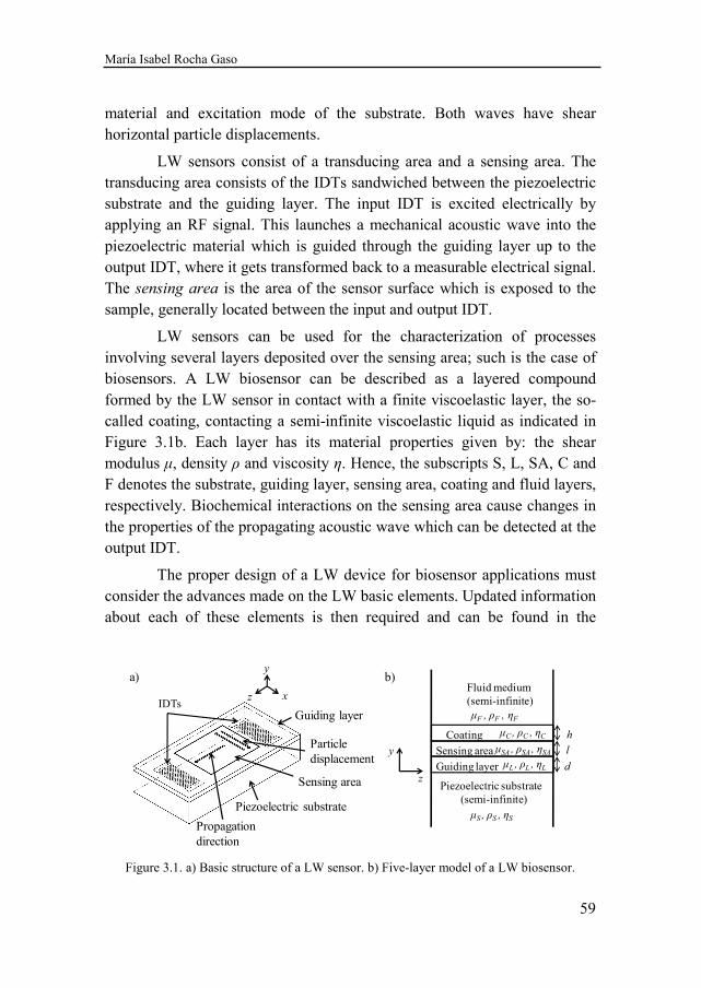
María Isabel Rocha Gaso
59
material and excitation mode of the substrate. Both waves have shear horizontal particle displacements.
LW sensors consist of a transducing area and a sensing area. The transducing area consists of the IDTs sandwiched between the piezoelectric substrate and the guiding layer. The input IDT is excited electrically by applying an RF signal. This launches a mechanical acoustic wave into the piezoelectric material which is guided through the guiding layer up to the output IDT, where it gets transformed back to a measurable electrical signal. The sensing area is the area of the sensor surface which is exposed to the sample, generally located between the input and output IDT.
LW sensors can be used for the characterization of processes involving several layers deposited over the sensing area; such is the case of biosensors. A LW biosensor can be described as a layered compound formed by the LW sensor in contact with a finite viscoelastic layer, the so-called coating, contacting a semi-infinite viscoelastic liquid as indicated in Figure 3.1b. Each layer has its material properties given by: the shear modulus µ, density ρ and viscosity η. Hence, the subscripts S, L, SA, C and F denotes the substrate, guiding layer, sensing area, coating and fluid layers, respectively. Biochemical interactions on the sensing area cause changes in the properties of the propagating acoustic wave which can be detected at the output IDT.
The proper design of a LW device for biosensor applications must consider the advances made on the LW basic elements. Updated information about each of these elements is then required and can be found in the
Figure 3.1. a) Basic structure of a LW sensor. b) Five-layer model of a LW biosensor.
Guiding layerIDTs
Propagation direction
Particle displacement
Sensing area
Piezoelectric substrate
Piezoelectric substrate(semi-infinite)
Guiding layer
Sensing area
Fluid medium(semi-infinite)
d
l
µF , ρF , ηF
µSA , ρSA , ηSA
µL , ρL , ηL
µS , ρS , ηS
a) b)
y
z
y
z x
Coating µC , ρC , ηC h
3. Contribution 1: LW sensors fundamentals. Optimization of the design specifications
60
following sections.
3.2.1 Piezoelectric substrate
Thanks to piezoelectricity, electrical charges can be generated by the imposition of mechanical stress. The phenomenon is reciprocal; applying an appropriate electrical field to a piezoelectric material generates a mechanical stress [163]. In LW sensors, an oscillating electric field is applied in the input IDT which, due to the piezoelectricity of the substrate, launches an acoustic wave. The wave propagates up to the output IDT where, again due to the piezoelectric properties of the substrate, is converted back to an electric signal. A remarkable parameter of the piezoelectric substrate is the electromechanical coupling coefficient (K2), which indicates the conversion efficiency from electric energy to mechanical energy; its value depends on the material properties. This is an important design parameter in LW sensors, since a higher K
2 leads to lower insertion loss LW devices [164] and, therefore, more sensitive LW sensors [165].
When choosing a material for the substrate of LW devices, apart from the desired low losses, other requirements, such as low temperature
coefficient of frequency (TCF) have to be considered as well. Special crystal cuts of the piezoelectric substrate material3 can yield an intrinsically temperature-compensated device which minimizes the influence of temperature on the sensor response, improving the LOD [166,167].
The shear horizontal polarization required for operation of the LW sensor in liquid media is another aspect to be considered when choosing the substrate material. In this sense, quartz is the only common substrate material that can be used to obtain a purely shear polarized wave [166]. The crystal cut and the wave propagation direction, which depends on the IDTs orientation, define the elastic, dielectric and piezoelectric constants of the crystal, and therefore the wave polarization. Possible cuts which generate a purely shear polarized wave are the AT-cut quartz and the ST-cut quartz.
3 The substrate crystal cuts (or plates) are obtained by cutting slices of a single-crystal starting material with an arbitrary orientation relative to the three orthogonal crystallographic axes.
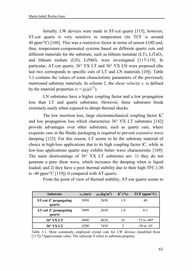
María Isabel Rocha Gaso
61
Initially, LW devices were made in ST-cut quartz [115], however, ST-cut quartz is very sensitive to temperature (its TCF is around 40 ppm/°C) [168]. This was a restrictive factor in terms of sensor LOD and, thus, temperature-compensated systems based on different quartz cuts and different materials for the substrate, such as lithium tantalate (LT), LiTaO3, and lithium niobate (LN), LiNbO3 were investigated [117-119]. In particular, AT-cut quartz, 36° YX LT and 36° YX LN were proposed (the last two corresponds to specific cuts of LT and LN materials [10]). Table 3.1 contains the values of some characteristic parameters of the previously mentioned substrate materials. In column 2, the shear velocity v, is defined by the material properties (v = (µ/ρ)1/2).
LN substrates have a higher coupling factor and a low propagation loss than LT and quartz substrates. However, these substrates break extremely easily when exposed to abrupt thermal shocks.
The low insertion loss, large electromechanical coupling factor K2 and low propagation loss which characterize 36° YX LT substrates [142] provide advantages over other substrates, such as quartz cuts, where exquisite care in the fluidic packaging is required to prevent excessive wave damping [123]. For this reason, LT seems to be the substrate material of choice in high-loss applications due to its high coupling factor K2, while in low-loss applications quartz may exhibit better wave characteristic [169]. The main shortcomings of 36° YX LT substrates are: 1) they do not generate a pure shear wave, which increases the damping when is liquid loaded; and 2) they have a poor thermal stability due to their high TFC (-30 to -40 ppm/°C [119]) if compared with AT-quartz. From the point of view of thermal stability, AT-cut quartz seems to
Substrate vS (m/s) ρS (kg/m3) K2 (%) TCF (ppm/°C)
ST-cut Z’ propagating quartz
5050 2650 1.9 40
AT-cut Z’ propagating quartz
5099 2650 1.4 0-1
36° YX LN 4800 4628 16 -75 to -80*
36° YX LT 4200 7454 5 -30 to -45
Table 3.1. Most commonly employed crystal cuts for LW devices (modified from [117]).*Approximate value. The subscript S refers to substrate property.
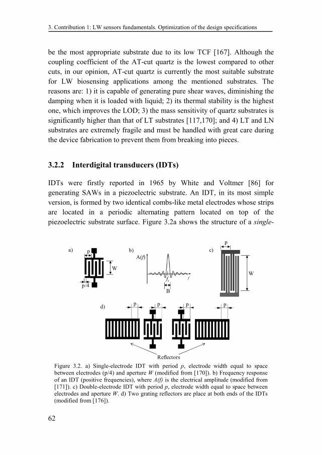
3. Contribution 1: LW sensors fundamentals. Optimization of the design specifications
62
be the most appropriate substrate due to its low TCF [167]. Although the coupling coefficient of the AT-cut quartz is the lowest compared to other cuts, in our opinion, AT-cut quartz is currently the most suitable substrate for LW biosensing applications among the mentioned substrates. The reasons are: 1) it is capable of generating pure shear waves, diminishing the damping when it is loaded with liquid; 2) its thermal stability is the highest one, which improves the LOD; 3) the mass sensitivity of quartz substrates is significantly higher than that of LT substrates [117,170]; and 4) LT and LN substrates are extremely fragile and must be handled with great care during the device fabrication to prevent them from breaking into pieces.
3.2.2 Interdigital transducers (IDTs)
IDTs were firstly reported in 1965 by White and Voltmer [86] for generating SAWs in a piezoelectric substrate. An IDT, in its most simple version, is formed by two identical combs-like metal electrodes whose strips are located in a periodic alternating pattern located on top of the piezoelectric substrate surface. Figure 3.2a shows the structure of a single-
Figure 3.2. a) Single-electrode IDT with period p, electrode width equal to space between electrodes (p/4) and aperture W (modified from [170]). b) Frequency response of an IDT (positive frequencies), where A(f) is the electrical amplitude (modified from [171]). c) Double-electrode IDT with period p, electrode width equal to space between electrodes and aperture W. d) Two grating reflectors are place at both ends of the IDTs (modified from [176]).
a) b)A(f)
f
B
p
p/8
W
c)
p p p pd)
Reflectors
fs
W
p/4
p
María Isabel Rocha Gaso
63
electrode IDT which consists of two strips per period p and acoustic
aperture W. The strip width is equal to the space between strips (p/4). One comb is connected to ground and the other to the center conductor of a coaxial cable where a RF signal is provided. A pair of two strips with different potential is called a finger pair.
The IDT electric equivalent circuit is explained in reference [171]. Figure 3.2b shows the IDT frequency response, where A(f) is the electrical amplitude of the RF signal. The maximum in A(f) occurs when the wavelength λ of the generated acoustic wave is equal to the period p and this arises at the so called synchronous frequency, fs. In relation to the bandwidth B of an IDT frequency response, this will be narrower when increasing the number of finger pairs, N. However, there is a limitation in the maximum N recommended, due to the fact that, in practice, when N exceeds 100, the losses associated with mass loading and the scattering from the electrodes increase. This neutralizes any additional advantage associated with the increase of the number of the finger pairs.
Due to symmetry of the IDT in the direction of propagation, the LW energy is emitted in equal amounts in opposite directions, giving an inherent loss of 3 dB. In a two-port device this factor contributes 6 dB to the total insertion loss [171,172].
Aluminum has been widely used as a material for IDTs and has been extensively demonstrated in literature as suitable for SAW generation. Aluminum resists corrosion and is the third most abundant element on Earth (after oxygen and silicon), which makes it low cost metal compared to other metals. Furthermore, aluminum IDTs vibre properly at high frequencies and diminish SAW damping [173]. The metallic layer of the electrodes must be thick enough to present a low electric resistance, but sufficiently thin to avoid an excessive mechanic charge for the acoustic wave (acoustic impedance breaking). Generally, a thickness between 100 and 200 nm of aluminum is employed.
There are a number of second-order effects, which are often significant in practice, that affect the transducer frequency response. The effect for which the transducer strips reflect surface waves causing mechanical and electrical perturbations of the surface is called electrode
interaction [30]. Usually, these unwanted reflections cancel each other over
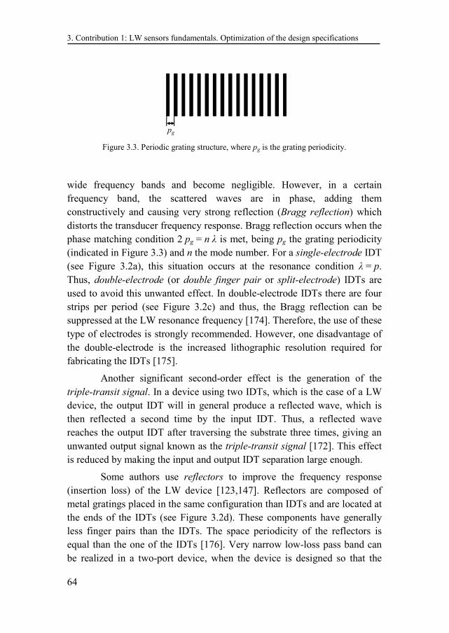
3. Contribution 1: LW sensors fundamentals. Optimization of the design specifications
64
wide frequency bands and become negligible. However, in a certain frequency band, the scattered waves are in phase, adding them constructively and causing very strong reflection (Bragg reflection) which distorts the transducer frequency response. Bragg reflection occurs when the phase matching condition 2 pg = n λ is met, being pg the grating periodicity (indicated in Figure 3.3) and n the mode number. For a single-electrode IDT (see Figure 3.2a), this situation occurs at the resonance condition λ = p. Thus, double-electrode (or double finger pair or split-electrode) IDTs are used to avoid this unwanted effect. In double-electrode IDTs there are four strips per period (see Figure 3.2c) and thus, the Bragg reflection can be suppressed at the LW resonance frequency [174]. Therefore, the use of these type of electrodes is strongly recommended. However, one disadvantage of the double-electrode is the increased lithographic resolution required for fabricating the IDTs [175].
Another significant second-order effect is the generation of the triple-transit signal. In a device using two IDTs, which is the case of a LW device, the output IDT will in general produce a reflected wave, which is then reflected a second time by the input IDT. Thus, a reflected wave reaches the output IDT after traversing the substrate three times, giving an unwanted output signal known as the triple-transit signal [172]. This effect is reduced by making the input and output IDT separation large enough.
Some authors use reflectors to improve the frequency response (insertion loss) of the LW device [123,147]. Reflectors are composed of metal gratings placed in the same configuration than IDTs and are located at the ends of the IDTs (see Figure 3.2d). These components have generally less finger pairs than the IDTs. The space periodicity of the reflectors is equal than the one of the IDTs [176]. Very narrow low-loss pass band can be realized in a two-port device, when the device is designed so that the
Figure 3.3. Periodic grating structure, where pg is the grating periodicity.
pg
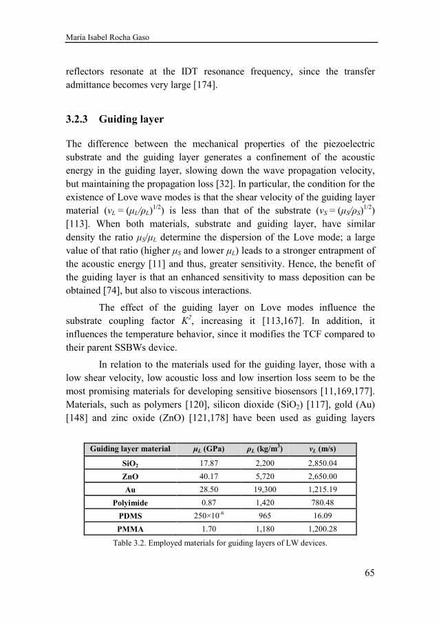
María Isabel Rocha Gaso
65
reflectors resonate at the IDT resonance frequency, since the transfer admittance becomes very large [174].
3.2.3 Guiding layer
The difference between the mechanical properties of the piezoelectric substrate and the guiding layer generates a confinement of the acoustic energy in the guiding layer, slowing down the wave propagation velocity, but maintaining the propagation loss [32]. In particular, the condition for the existence of Love wave modes is that the shear velocity of the guiding layer material (vL = (µL/ρL)
1/2) is less than that of the substrate (vS = (µS/ρS)1/2)
[113]. When both materials, substrate and guiding layer, have similar density the ratio µS/µL determine the dispersion of the Love mode; a large value of that ratio (higher µS and lower µL) leads to a stronger entrapment of the acoustic energy [11] and thus, greater sensitivity. Hence, the benefit of the guiding layer is that an enhanced sensitivity to mass deposition can be obtained [74], but also to viscous interactions.
The effect of the guiding layer on Love modes influence the substrate coupling factor K
2, increasing it [113,167]. In addition, it influences the temperature behavior, since it modifies the TCF compared to their parent SSBWs device.
In relation to the materials used for the guiding layer, those with a low shear velocity, low acoustic loss and low insertion loss seem to be the most promising materials for developing sensitive biosensors [11,169,177]. Materials, such as polymers [120], silicon dioxide (SiO2) [117], gold (Au) [148] and zinc oxide (ZnO) [121,178] have been used as guiding layers
Guiding layer material µL (GPa) ρL (kg/m3) vL (m/s)
SiO2 17.87 2,200 2,850.04
ZnO 40.17 5,720 2,650.00
Au 28.50 19,300 1,215.19
Polyimide 0.87 1,420 780.48
PDMS 250×10-6 965 16.09
PMMA 1.70 1,180 1,200.28
Table 3.2. Employed materials for guiding layers of LW devices.
3. Contribution 1: LW sensors fundamentals. Optimization of the design specifications
66
[123]. In Table 3.2 some properties of these materials are presented4. The use of polymers (like Novolac®, polyimide, polydimethylsiloxane (PDMS) and polymethylmethacrylate (PMMA)) is interesting from the point of view of the sensitivity, since they have low shear velocity. Additionally, some polymers, like Novolac photoresist, are very resistant to chemical agents [157,179]. However, polymers have high acoustic damping (losses) [179] and this is a clear disadvantage for biosensing application.
Guiding layer/substrate structures made with ZnO as the guiding layer have some advantages over those with a different material. This is the case of ZnO/ST-quartz structure, for which significantly high sensitivity, small TCF and high K
2 were reported [178]. ZnO/LT devices were also found to have higher mass sensitivity than SiO2/LT [170]. However, ZnO has several disadvantages: it is CMOS contaminant, a semiconductor, and thus, it can deteriorate the efficiency of the transducers and make some artifacts. In addition, it gets easily rough when sputtered and it is very reactive with acids, liquids, or moisture, so it will dissolve if exposed to water or humid environment, which is a big problem in biosensors application. Regarding Au guiding layers, they provide very strong wave guiding, since Au has a relatively low shear acoustic velocity and a high density. However, it couples the RF signals of the IDTs.
Silicon dioxide (SiO2) -also known as fused silica- is a standard material in semiconductor industry and offers low damping, sufficient low shear velocity and excellent chemical and mechanical resistance [180]. It is the only native oxide of a common semiconductor which is stable in water and at elevated temperatures, an excellent electrical insulator, a mask to common diffusing species, and capable of forming a nearly perfect electrical interface with its substrate. When SiO2 is needed on materials other than silicon, it is obtained by chemical vapor deposition (CVD), either thermal CVD or Plasma enhanced CVD (PECVD) [181]. The main shortcoming for SiO2 is that the optimum thickness, at which the maximum sensitivity is reached, is very high (see Section 3.5), so this complicates the manufacturing process. Nevertheless, at the present, we consider that SiO2 is the most appropriate material for LW biosensors guiding layer, mainly due to its low damping and excellent chemical and mechanical properties [181] 4 These values are for guidance, since for deposited or grown materials these values depend on the desposition technique and for polymers layers on the cure process.
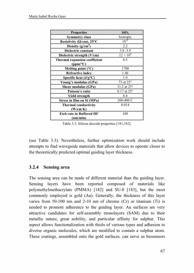
María Isabel Rocha Gaso
67
(see Table 3.3). Nevertheless, further optimization work should include attempts to find waveguide materials that allow devices to operate closer to the theoretically predicted optimal guiding layer thickness.
3.2.4 Sensing area
The sensing area can be made of different material than the guiding layer. Sensing layers have been reported composed of materials like polymethylmethacrylate (PMMA) [182] and SU-8 [183], but the most commonly employed is gold (Au). Generally, the thickness of this layer varies from 50-100 nm and 2-10 nm of chrome (Cr) or titanium (Ti) is needed to promote adherence to the guiding layer. Au surfaces are very attractive candidates for self-assembly monolayers (SAM) due to their metallic nature, great nobility, and particular affinity for sulphur. This aspect allows functionalization with thiols of various types and adhesion to diverse organic molecules, which are modified to contain a sulphur atom. These coatings, assembled onto the gold surfaces, can serve as biosensors
Properties SiO2
Symmetry class Isotropic Resistivity (Ω-cm), 25°C 1016
Density (g/cm3) 2.2 Dielectric constant 3.8 -3.9
Dielectric strength (V/cm) 12 × 106
Thermal expansion coefficient (ppm/°C)
0.5
Melting point (°C) 1700 Refractive index 1.46
Specific heat (J/g°C) 1.0 Young’s modulus (GPa) 73 at 25°
Shear modulus (GPa) 31.2 at 25° Poisson’s ratio 0.17 at 25° Yield strength 8.4
Stress in film on Si (MPa) 200-400 C Thermal conductivity
(W/cm K) 0.014
Etch rate in Buffered HF (nm/min)
100
Table 3.3. Silicon dioxide properties [181,182].
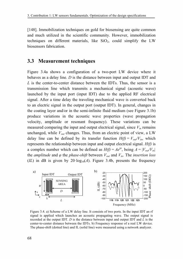
3. Contribution 1: LW sensors fundamentals. Optimization of the design specifications
68
[148]. Immobilization techniques on gold for biosensing are quite common and much utilized in the scientific community. However, immobilization techniques on different materials, like SiO2, could simplify the LW biosensors fabrication.
3.3 Measurement techniques
Figure 3.4a shows a configuration of a two-port LW device where it behaves as a delay line. D is the distance between input and output IDT and L is the center-to-center distance between the IDTs. Thus, the sensor is a transmission line which transmits a mechanical signal (acoustic wave) launched by the input port (input IDT) due to the applied RF electrical signal. After a time delay the traveling mechanical wave is converted back to an electric signal in the output port (output IDT). In general, changes in the coating layer and/or in the semi-infinite fluid medium (see Figure 3.1b) produce variations in the acoustic wave properties (wave propagation velocity, amplitude or resonant frequency). These variations can be measured comparing the input and output electrical signal, since Vin remains unchanged, while Vout changes. Thus, from an electric point of view, a LW delay line can be defined by its transfer function H(f) = Vout/Vin, which represents the relationship between input and output electrical signal. H(f) is a complex number which can be defined as H(f) = Ae
jφ, being A = |Vout/Vin| the amplitude and φ the phase-shift between Vout and Vin. The insertion loss (IL) in dB is given by 20·log10(A). Figure 3.4b, presents the frequency
Figure 3.4. a) Scheme of a LW delay line. It consists of two ports. In the input IDT an rf signal is applied which launches an acoustic propagating wave. The output signal is recorded at the output IDT. D is the distance between input and output IDT and L is the center-to-center distance between the IDTs. b) Frequency response of a real LW device. The phase-shift (dotted line) and IL (solid line) were measured using a network analyzer.
D
SENSING AREA
Input IDT Output IDT
W
Lλz
x
118 119 120 121 122 123-100
-90
-80
-70
-60
-50
-40
-30
-20
118 119 120 121 122 123-200
-150
-100
-50
0
50
100
150
200
Frequency (MHz)
a)
IL (
dB)
Pha
se s
hift
(D
EG
)
b)
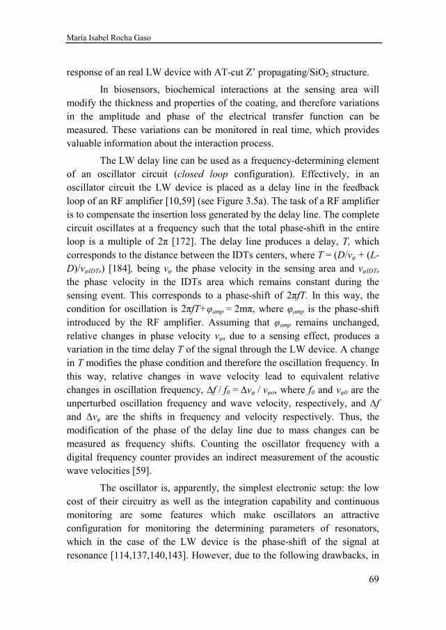
María Isabel Rocha Gaso
69
response of an real LW device with AT-cut Z’ propagating/SiO2 structure.
In biosensors, biochemical interactions at the sensing area will modify the thickness and properties of the coating, and therefore variations in the amplitude and phase of the electrical transfer function can be measured. These variations can be monitored in real time, which provides valuable information about the interaction process.
The LW delay line can be used as a frequency-determining element of an oscillator circuit (closed loop configuration). Effectively, in an oscillator circuit the LW device is placed as a delay line in the feedback loop of an RF amplifier [10,59] (see Figure 3.5a). The task of a RF amplifier is to compensate the insertion loss generated by the delay line. The complete circuit oscillates at a frequency such that the total phase-shift in the entire loop is a multiple of 2π [172]. The delay line produces a delay, T, which corresponds to the distance between the IDTs centers, where T = (D/vφ + (L-D)/vφIDTs) [184], being vφ the phase velocity in the sensing area and vφIDTs the phase velocity in the IDTs area which remains constant during the sensing event. This corresponds to a phase-shift of 2πfT. In this way, the condition for oscillation is 2πfT+φamp = 2mπ, where φamp is the phase-shift introduced by the RF amplifier. Assuming that φamp remains unchanged, relative changes in phase velocity vφ, due to a sensing effect, produces a variation in the time delay T of the signal through the LW device. A change in T modifies the phase condition and therefore the oscillation frequency. In this way, relative changes in wave velocity lead to equivalent relative changes in oscillation frequency, ∆f / f0 = ∆vφ / vφo, where f0 and vφ0 are the unperturbed oscillation frequency and wave velocity, respectively, and ∆f and ∆vφ are the shifts in frequency and velocity respectively. Thus, the modification of the phase of the delay line due to mass changes can be measured as frequency shifts. Counting the oscillator frequency with a digital frequency counter provides an indirect measurement of the acoustic wave velocities [59].
The oscillator is, apparently, the simplest electronic setup: the low cost of their circuitry as well as the integration capability and continuous monitoring are some features which make oscillators an attractive configuration for monitoring the determining parameters of resonators, which in the case of the LW device is the phase-shift of the signal at resonance [114,137,140,143]. However, due to the following drawbacks, in
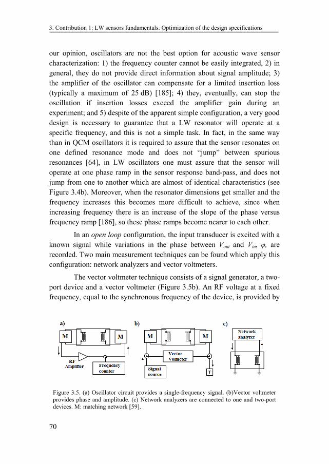
3. Contribution 1: LW sensors fundamentals. Optimization of the design specifications
70
our opinion, oscillators are not the best option for acoustic wave sensor characterization: 1) the frequency counter cannot be easily integrated, 2) in general, they do not provide direct information about signal amplitude; 3) the amplifier of the oscillator can compensate for a limited insertion loss (typically a maximum of 25 dB) [185]; 4) they, eventually, can stop the oscillation if insertion losses exceed the amplifier gain during an experiment; and 5) despite of the apparent simple configuration, a very good design is necessary to guarantee that a LW resonator will operate at a specific frequency, and this is not a simple task. In fact, in the same way than in QCM oscillators it is required to assure that the sensor resonates on one defined resonance mode and does not “jump” between spurious resonances [64], in LW oscillators one must assure that the sensor will operate at one phase ramp in the sensor response band-pass, and does not jump from one to another which are almost of identical characteristics (see Figure 3.4b). Moreover, when the resonator dimensions get smaller and the frequency increases this becomes more difficult to achieve, since when increasing frequency there is an increase of the slope of the phase versus frequency ramp [186], so these phase ramps become nearer to each other.
In an open loop configuration, the input transducer is excited with a known signal while variations in the phase between Vout and Vin, φ, are recorded. Two main measurement techniques can be found which apply this configuration: network analyzers and vector voltmeters.
The vector voltmeter technique consists of a signal generator, a two-port device and a vector voltmeter (Figure 3.5b). An RF voltage at a fixed frequency, equal to the synchronous frequency of the device, is provided by
Figure 3.5. (a) Oscillator circuit provides a single-frequency signal. (b)Vector voltmeter provides phase and amplitude. (c) Network analyzers are connected to one and two-port devices. M: matching network [59].
María Isabel Rocha Gaso
71
the signal generator to the input IDT. The changes in signal amplitude and phase-shift between the input and output IDTs are monitored by the vector voltmeter. Changes in phase-shift indicate changes in wave velocity, while changes in amplitude indicate changes in the attenuation of the wave.
The advantage of this electronic setup is that it provides velocity and amplitude information about the signal and avoids the disadvantages of a limited amplifier gain. On the other hand, phase measurements with commercially available vector voltmeters are 10 to 100 times less sensitive to velocity changes than frequency measurements by the oscillator setup.
It is also possible to use a vector voltmeter in a phase-locked loop. In this case the phase is maintained constant by adjusting the frequency and the changes in frequency can be monitored [59].
The network analyzer is the instrument of choice to measure frequency responses of either one- or two-port devices, due to the fact that this setup allows a complete characterization of the devices under all conditions, including those for which the oscillator method fails. For two-port devices (see Figure 3.5c) the network analyzer records the transmitted signal to obtain the impedance characteristics of the device. Therefore, it works in the same way that a signal generator/vector voltmeter configuration being possible to measure amplitude and phase information of the signal as a function of the input frequency. Frequency scans can also be made during experiments to determine the device response as a function of time [59].
Network analyzers are the most commonly used instrumentation to characterize LW delay lines in open loop configurations. Nevertheless, recently, some authors successfully validated a new characterization technique for QCM sensors based on the open loop configuration [187]. In this technique, which can be considered as a variation of the vector voltmeter technique, the input transducer is excited at a fixed frequency while the phase-shift between Vout and Vin is recorded. In this configuration, in the absence of interferences, phase variations measured experimentally can be related to changes in the physical properties of the layers deposited over the sensing area [11]. A read-out circuit based on this technique for high frequency liquid loaded QCM devices was developed and tested by the same authors [188]. The main advantages of this read-out circuit are: its low
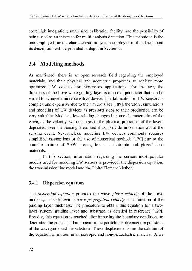
3. Contribution 1: LW sensors fundamentals. Optimization of the design specifications
72
cost; high integration; small size; calibration facility; and the possibility of being used as an interface for multi-analysis detection. This technique is the one employed for the characterization system employed in this Thesis and its description will be provided in depth in Section 5.
3.4 Modeling methods
As mentioned, there is an open research field regarding the employed materials, and their physical and geometric properties to achieve more optimized LW devices for biosensors applications. For instance, the thickness of the Love-wave guiding layer is a crucial parameter that can be varied to achieve a more sensitive device. The fabrication of LW sensors is complex and expensive due to their micro sizes [189]; therefore, simulations and modeling of LW devices as previous steps to their production can be very valuable. Models allow relating changes in some characteristics of the wave, as the velocity, with changes in the physical properties of the layers deposited over the sensing area, and thus, provide information about the sensing event. Nevertheless, modeling LW devices commonly requires simplified assumptions or the use of numerical methods [170] due to the complex nature of SAW propagation in anisotropic and piezoelectric materials. In this section, information regarding the current most popular models used for modeling LW sensors is provided: the dispersion equation, the transmission line model and the Finite Element Method.
3.4.1 Dispersion equation
The dispersion equation provides the wave phase velocity of the Love mode, vφ, –also known as wave propagation velocity- as a function of the guiding layer thickness. The procedure to obtain this equation for a two-layer system (guiding layer and substrate) is detailed in reference [129]. Broadly, this equation is reached after imposing the boundary conditions to determine the constants that appear in the particle displacement expressions of the waveguide and the substrate. These displacements are the solution of the equation of motion in an isotropic and non-piezoelectric material. After
María Isabel Rocha Gaso
73
extensive algebraic manipulation [129], the dispersion equation for a two-layer system is found, resulting [190]:
( ) ( )( )
2 2
2 2
1tan
1
SSLy
L L
v vk d
v v
ϕ
ϕ
µµ
−=
− (3.1)
where kLy is the guiding layer transverse wavenumber in y direction (see Figure 3.1a), given by:
2 2
2 2Ly
L
kv vϕ
ω ω= − (3.2)
Taking into account the relation between the frequency and wave wavelength, f = vφ/λ, the argument of the tangent in Eq.(3.1) can be written as:
2 2
1 12Ly
L
dk d v
v vϕ
ϕ
πλ
= − (3.3)
where the ratio d/λ is the normalized guiding layer thickness.
From the dispersion equation, the phase velocity can be solved numerically as a function of the normalized guiding layer thickness and of the physical properties of the substrate and guiding layer.
On the other hand, the group velocity, vg, as a function of the normalized guiding layer thickness can also be determined from the phase velocity by the equation [177]:
( )d
1dg
vdv v
v d
ϕϕ
ϕ
λλ
= +
(3.4)
The phase velocity and group velocity of an AT-cut quartz/SiO2 Z’ propagating layered structure were calculated using the dispersion equation (Eq. (3.1)) solved numerically using the bisection method, and Eq. (3.4) respectively (see Script 1 in Appendix G). The data used to calculate vφ and vg for this LW structure were: vS = 5099 m/s, ρS = 2650 kg/m3, vL = 2850 m/s, ρL = 2200 kg/m3 and λ = 40 µm. The respective shear modulus were obtained through µi = vi
2 ρi, where i represents a given material. The results are depicted in Figure 3.6. This figure provides information about the changes in the wave phase and group velocities due to
3. Contribution 1: LW sensors fundamentals. Optimization of the design specifications
74
changes in the guiding layer thickness. Assuming that the perturbing mass layer deposited over the sensing area is of the same material than the guiding layer, this equation will provide information over the sensing event. Nevertheless, this assumption is far from the biosensors reality, where the consideration of a five–layer model is required (see Figure 3.1b).
The phase velocity provided by the dispersion equation can be used to determine the optimal guiding layer thickness, which provides a maximum sensitivity. This issue will be addressed in Section 3.5.
Mc Hale et al. developed the dispersion equation of three and four-layer systems neglecting piezoelectricity of the substrate [74]. When the substrate piezoelectricity is not considered, the dispersion equation is simplified. This can be the case of quartz substrates, whose piezoelectricity is low. However, as the piezoelectricity of a substrate increases (like in the case of LT and LN), neglecting piezoelectricity, or assuming it is accounted for a stiffening effect in the phase velocity, may be less valid [191]. Liu et al. provided a theoretical model for analyzing the LW in a multilayered structure over a piezoelectric substrate [191]. The analytical form of the complex dispersion equation when a LW device is loaded with a viscous (Newtonian) liquid was obtained by Kiełczynski et al. [192]. Nevertheless, in our opinion, for those applications with a high number of layers, as in the case of biosensors, the use of the transmission line model is more convenient, since it is a very structured and intuitive model where the addition of an extra layer does not make the procedure more complex. From the programming point of view, this is an enormous advantage.
Figure 3.6. a) AT-cut Z’ propagating quartz/SiO2 phase velocity (continuous line) and group velocity (dotted line) for λ = 40 µm.
d/λ
Vel
ocit
y (m
/s)
0 0.2 0.4 0.6 0.8 12500
3000
3500
4000
4500
5000
5500
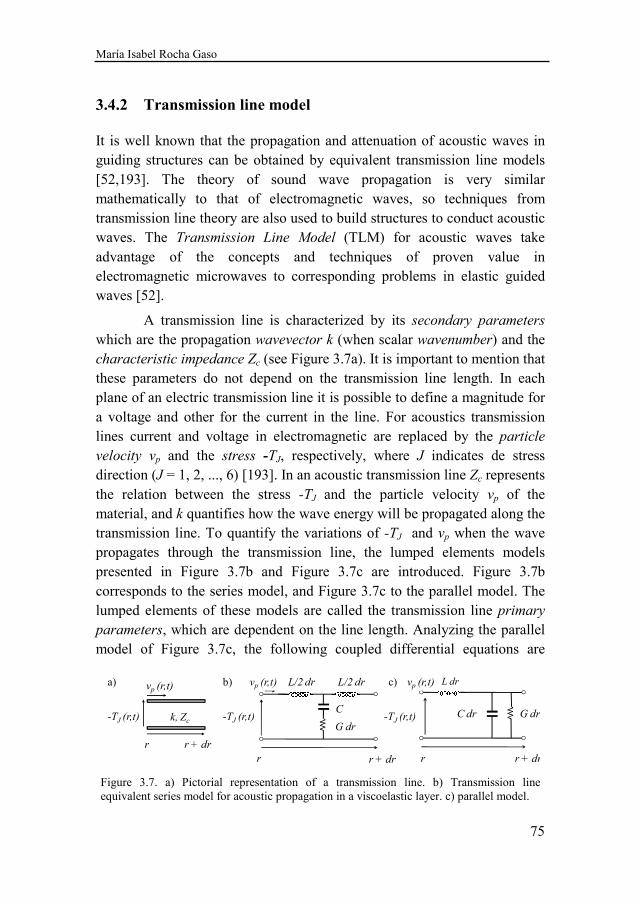
María Isabel Rocha Gaso
75
Figure 3.7. a) Pictorial representation of a transmission line. b) Transmission line equivalent series model for acoustic propagation in a viscoelastic layer. c) parallel model.
C dr
L/2 dr L/2 dr
G dr
vp
r r + dr
+
-
TJ
vp (r,t)a)
k, Zc-TJ (r,t)
vp (r,t)
r r + dr
b) b.2)
C dr
L dr
G dr
vp
r r + dr
TJ
+
-
-TJ (r,t)
r r + dr
L/2 dr L/2 dr
C
drG dr
c)
-TJ (r,t)
L dr
C dr G dr
r r + dr
vp (r,t)
3.4.2 Transmission line model
It is well known that the propagation and attenuation of acoustic waves in guiding structures can be obtained by equivalent transmission line models [52,193]. The theory of sound wave propagation is very similar mathematically to that of electromagnetic waves, so techniques from transmission line theory are also used to build structures to conduct acoustic waves. The Transmission Line Model (TLM) for acoustic waves take advantage of the concepts and techniques of proven value in electromagnetic microwaves to corresponding problems in elastic guided waves [52].
A transmission line is characterized by its secondary parameters which are the propagation wavevector k (when scalar wavenumber) and the characteristic impedance Zc (see Figure 3.7a). It is important to mention that these parameters do not depend on the transmission line length. In each plane of an electric transmission line it is possible to define a magnitude for a voltage and other for the current in the line. For acoustics transmission lines current and voltage in electromagnetic are replaced by the particle
velocity vp and the stress -TJ, respectively, where J indicates de stress direction (J = 1, 2, ..., 6) [193]. In an acoustic transmission line Zc represents the relation between the stress -TJ and the particle velocity vp of the material, and k quantifies how the wave energy will be propagated along the transmission line. To quantify the variations of -TJ and vp when the wave propagates through the transmission line, the lumped elements models presented in Figure 3.7b and Figure 3.7c are introduced. Figure 3.7b corresponds to the series model, and Figure 3.7c to the parallel model. The lumped elements of these models are called the transmission line primary
parameters, which are dependent on the line length. Analyzing the parallel model of Figure 3.7c, the following coupled differential equations are
3. Contribution 1: LW sensors fundamentals. Optimization of the design specifications
76
obtained:
( )( )
( )( )
Jp
pJ
dT rZ v r
dr
dv rY T r
dr
= ⋅
= ⋅
(3.5)
where Z=jωL, Y=jωC+G and ω=2πf. Being Z, L, Y, C, G, f, the impedance, inductance, admittance, capacitance and conductance per unit of length, respectively and f the frequency of TJ and vp. Deriving a second time we obtain:
2
2
2
2
( )( )
( )( )
JJ
pp
d T rZ Y T r
dr
d v rZ Y v r
dr
= ⋅ ⋅
= ⋅ ⋅
(3.6)
The solutions for these equations are given by:
( )
( )
r rJ J J
r rJ Jp
c c
T r T e T e
T Tv r e e
Z Z
γ γ
γ γ
+ − ⋅ − ⋅
+ −− ⋅ ⋅
= +
= − (3.7)
where TJ+ and TJˉ are arbitrary values for the intensity of the incident an
reflected waves, respectively. The linear propagation exponent or complex
propagation factor, γ, is directly related to the wavevector (γ=jk) and is given by γ = (ZY)1/2
= α + jβ. The real part of γ, denoted as the attenuation
coefficient, α, represents the attenuation suffered by the wave when propagating through the transmission line. The imaginary part of γ, denoted as the phase coefficient, β, when multiplied by a distance, quantifies the phase-shift that the wave suffers when traveling that distance. The characteristic impedance of the line Zc establishes the relationship between the stress TJ and the particle velocity vp in this way: Zc = (-TJ/vp) and it is also given by Zc=(Z/Y)1/2. First row of Table 3.4 shows the relationships between primary and secondary parameters of a transmission line for the series and parallel model.
The relation between the secondary (or primary) parameters and the properties of the transmission line materials is achieved by comparing Eqs. (3.5) with the motion equations of the LW assuming isotropic layers [193]. These relations are given in the second row of Table 3.4 for the series and
María Isabel Rocha Gaso
77
parallel model and the procedure for obtaining these relations is explained next.
The acoustic field equation for an isotropic lossless solid is given by [193]:
pvT F
tρ
∂∇ ⋅ = −
∂ (3.8)
where, ∇⋅ is the divergence, T is the stress vector, ρ is the material density, vp is the particle velocity vector and F is the external force vector. Developing last equation in rectangular coordinates we have:
1
2
3
4
5
6
0 0 0
0 0 0
0 0 0
px x
py y
pz z
T
Tx z y v FT
v FTy z x t
v FT
z y x T
ρ
∂ ∂ ∂ ∂ ∂ ∂ ∂ ∂ ∂ ∂
= − ∂ ∂ ∂ ∂ ∂ ∂ ∂
∂ ∂ ∂
(3.9)
In the LW structure described in Figure 3.1 the shear horizontal particle displacements occur only in x direction, therefore, vpy = vpz = 0. Moreover, there is no variation of the stress in the x direction (see Figure
3.1), thus 0x∂ ∂ = , and there is not external forces applied to the solid.
Under these conditions, Eq. (3.9) becomes:
Series model Parallel model
1 /
c
LCk j
j C G
L LZ j
C G
γ ωω
ω
= − =+
= +
( )
c
k j j j L G j C
j LZ
G j C
γ ω ω
ωω
= − = − +
=+
1
1
C
G
L
µ
ηρ
=
=
=
2 2 2
2
2 2 2
C
G
L
µω η µ
ηωω η µρ
=+
=+
=
Table 3.4. Equivalent transmission line model parameters in terms of the layer properties.
3. Contribution 1: LW sensors fundamentals. Optimization of the design specifications
78
1
2
3
4
5
6
0 0 0 0
0 0 0 0 0
0
0 0 0 0
px
T
Tz y vT
Ty z t
T
z y T
ρ
∂ ∂ ∂ ∂ ∂ ∂ ∂
= ∂ ∂ ∂ ∂ ∂
∂ ∂
(3.10)
Operating Eq. (3.10) we obtain the following equations:
5 6( , )( , ) ( , ) pxv y zT y z T y z
z y tρ
∂∂ ∂+ =
∂ ∂ ∂ (3.11)
2 4( , ) ( , )0
T y z T y z
y z
∂ ∂+ =
∂ ∂ (3.12)
3 4( , ) ( , )0
T y z T y z
z y
∂ ∂+ =
∂ ∂ (3.13)
Eq. (3.11) constitutes the first equation of motion of the particles in a solid. The second equation of motion is obtained using the expression that relates the components of stress as general linear functions of all the strain components which is given by [193]:
:T c S= (3.14)
where c is the matrix of elastic stiffness constants of the material and S is the strain vector. Developing Eq. (3.14) we obtain:
1 11 1 12 2 13 3 14 4 15 5 16 6
2 21 1 22 2 23 3 24 4 25 5 26 6
3 31 1 32 2 33 3 34 4 35 5 36 6
4 41 1 42 2 43 3 44 4 45 5 46 6
5 51 1 52 2 53 3 54 4 55 5 56 6
6 61 1
T c S c S c S c S c S c S
T c S c S c S c S c S c S
T c S c S c S c S c S c S
T c S c S c S c S c S c S
T c S c S c S c S c S c S
T c S c
= + + + + +
= + + + + +
= + + + + +
= + + + + +
= + + + + +
= + 62 2 63 3 64 4 65 5 66 6S c S c S c S c S+ + + +
(3.15)
where, the strain components S1, S2, S3, S4, S5, and S6, corresponds to Sxx, Syy,
Szz, 2Syz, 2Sxz, and 2Sxy [193], respectively. These components are given by:
1, , ,
2
jiij
uuS i j x y z
j i
∂ ∂= + =
∂ ∂ (3.16)
María Isabel Rocha Gaso
79
Therefore for the LW structure in Figure 3.1, S1, S2, S3, S4 are all
equal to zero, since 0x∂ ∂ = , uy = 0 and uz = 0. Then, the strain components
of the LW structure are:
1 2 3 4
5
6
0
x
x
S S S S
uS
z
uS
y
= = = =
∂=
∂∂
=∂
(3.17)
Substituting Eqs. (3.17) into Eqs. (3.15) and considering the matrix of elastic stiffness constants of an isotropic material (see Appendix D) the following equations are obtained:
5 44
6 44
( , )( , )
( , )( , )
x
x
u y zT y z c
z
u y zT y z c
y
∂=
∂∂
=∂
(3.18)
Deriving Eq. (3.18) with respect to time gives:
5
44
644
( , )( , )
( , )( , )
px
px
v y zT y zc
t z
v y zT y zc
t y
∂∂=
∂ ∂∂∂
=∂ ∂
(3.19)
Last equations were obtained assuming a lossless isotropic medium. In order to consider material losses this substitution has to be made in last equation equations [192]: c44 → c44 + jωη44, resulting the following equations:
( ) ( )( )
( ) ( )( )
544 44
644 44
,,
,,
px
px
v y zT y zc j
t z
v y zT y zc j
t y
ωη
ωη
∂∂= +
∂ ∂∂∂
= +∂ ∂
(3.20)
The equations of Eq. (3.20) constitute the second equation of motion of the particles in a solid.
Thus, from Eq. (3.11) and Eq. (3.20) the constitutive equations of particle motion in a solid can be written as:
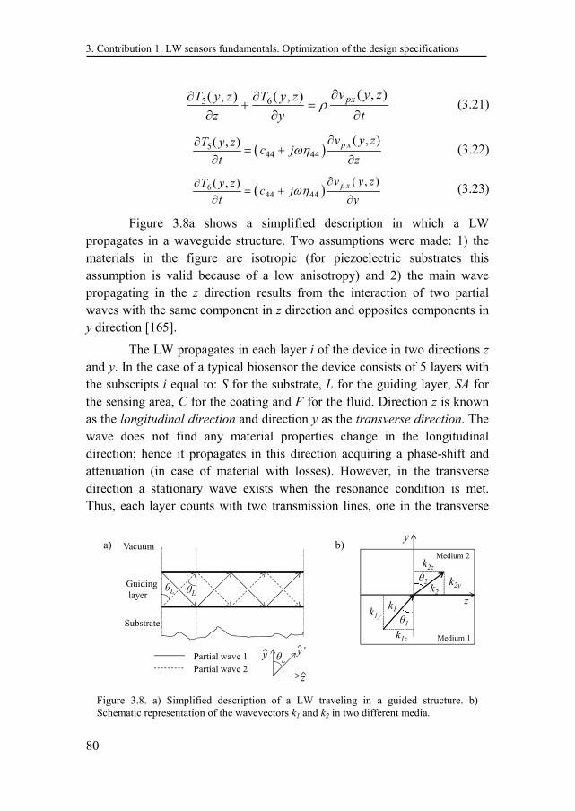
3. Contribution 1: LW sensors fundamentals. Optimization of the design specifications
80
5 6( , )( , ) ( , ) pxv y zT y z T y z
z y tρ
∂∂ ∂+ =
∂ ∂ ∂ (3.21)
( )544 44
( , )( , ) p xv y zT y zc j
t zωη
∂∂= +
∂ ∂ (3.22)
( )644 44
( , )( , ) p xv y zT y zc j
t yωη
∂∂= +
∂ ∂ (3.23)
Figure 3.8a shows a simplified description in which a LW propagates in a waveguide structure. Two assumptions were made: 1) the materials in the figure are isotropic (for piezoelectric substrates this assumption is valid because of a low anisotropy) and 2) the main wave propagating in the z direction results from the interaction of two partial waves with the same component in z direction and opposites components in y direction [165].
The LW propagates in each layer i of the device in two directions z and y. In the case of a typical biosensor the device consists of 5 layers with the subscripts i equal to: S for the substrate, L for the guiding layer, SA for the sensing area, C for the coating and F for the fluid. Direction z is known as the longitudinal direction and direction y as the transverse direction. The wave does not find any material properties change in the longitudinal direction; hence it propagates in this direction acquiring a phase-shift and attenuation (in case of material with losses). However, in the transverse direction a stationary wave exists when the resonance condition is met. Thus, each layer counts with two transmission lines, one in the transverse
Figure 3.8. a) Simplified description of a LW traveling in a guided structure. b) Schematic representation of the wavevectors k1 and k2 in two different media.
Guidinglayer
Substrate
Vacuum
θL θL
θL
z
y y’Partial wave 1Partial wave 2
y
z
θ1
k1z
k1y
k1
Medium 1
Medium 2
k2
k2z
k2yθ2
a) b)
María Isabel Rocha Gaso
81
direction and the other in the longitudinal direction. When a wave propagates in y’ direction (see Figure 3.8a), as it happens with the partial waves of a layer i, ki has that same direction (see Figure 3.8b), and therefore, it has components in z and y directions. In this way, the secondary parameters of each transmission line are determined from the projection of the parameter in the proper direction. The relation between the wavevector and the wave velocity is ki=ω/vi. Hence, ki and vi have the same direction and the wave velocity in y’ direction also has components in z and y.
Since y = y’ cos θi and z = y’ sin θi, the spatial derivatives expressed for y’ are given by:
cos' i
y yθ
∂ ∂=
∂ ∂ (3.24)
sin' i
z yθ
∂ ∂=
∂ ∂ (3.25)
where the angles θi are called complex coupling angles of a layer i.
Defining T5’(y’) = T5(y, z)sin θi+T6(y, z)cos θi, and deriving the expression with respect to y’, we obtain the following equation:
( ) ( ) ( )5' 5 6' , ,
sin cos' ' 'i i
T y T y z T y z
y y yθ θ
∂ ∂ ∂= +
∂ ∂ ∂ (3.26)
which can be simplified applying Eqs. (3.25) and (3.24) resulting:
( ) ( ) ( )5' 5 6' , ,
'
T y T y z T y z
y z y
∂ ∂ ∂= +
∂ ∂ ∂ (3.27)
Comparing Eq. (3.27) with Eq. (3.21) we obtain:
( ) ( )5' ''
'pxv yT y
y tρ
∂∂=
∂ ∂ (3.28)
Since Eq. (3.28) is time-harmonic, this equation can be written as:
5'( ')( ')
' px
T yj v y
yω ρ
∂=
∂ (3.29)
which represents the first equation of motion of a partial wave propagating in y’ direction.
3. Contribution 1: LW sensors fundamentals. Optimization of the design specifications
82
Combining Eq. (3.22) and Eq. (3.23) the second equation of motion of a partial wave in y’ direction is obtained. Multiplying Eq. (3.22) by sin θi and Eq. (3.23) by cos θi is obtained:
( ) ( )( )
( ) ( )( )
544 44
644 44
,,sin sin
,,cos cos
pxi i
pxi i
v y zT y zc j
t z
v y zT y zc j
t y
θ ωη θ
θ ωη θ
∂∂= +
∂ ∂∂∂
= +∂ ∂
(3.30)
Adding both expressions results in:
( ) ( ) ( ) ( )5 644 44
, ,sin cos sin cos ,i i i i px
T y z T y zc j v y z
t t z yθ θ ωη θ θ
∂ ∂ ∂ ∂+ = + + ∂ ∂ ∂ ∂
(3.31)
Multiplying Eq. (3.24) by cos θi and Eq. (3.25) by sin θi and adding such equations is obtained:
cos sin'i i
y z yθ θ
∂ ∂ ∂+ =
∂ ∂ ∂ (3.32)
Substituting this last equation and Eq. (3.26) in Eq. (3.31) results in:
( ) ( )( )
5' 44 44
''
'pxv y
j T y c jy
ω ωη∂
= +∂
(3.33)
which constitutes the second equation of motion of a partial wave in y’ direction.
Comparing Eqs. (3.29) and (3.33) with the transmission line equations (Eq.(3.5)) for r = y’ and J = 5’:
( ) ( ) ( ) ( )
( ) ( )( ) ( )
( ) ( )
5' 5'
5' 44 44 5'
' '' '
' '
' '' '
' '
px px
px px
T y T yj v y j Lv y
y y
v y v yj T y c j G j C T y
y y
ωρ ω
ω ωη ω
∂ ∂= → =
∂ ∂
∂ ∂= + → = +
∂ ∂
(3.34)
the following relations can be observed:
( ) ( )
244 44
2 22 244 44 44 44
; ;c
L C Gc c
ω ηρ
ωη ωη= = =
+ + (3.35)
María Isabel Rocha Gaso
83
Eq. (3.35) provides the relation between the primary parameters and the properties of the transmission line materials. Using the relations given in the first row of Table 3.4, the relations between the secondary parameters of the transmission line and the material properties (ρ, c44, η44) that compose it can be found:
( )( )44 44
4444 44
;cZ c j kc j c
ω ωρ ωη
ωη ρ ρ= + = =
+ (3.36)
In the previous equation 44c ρ corresponds to the wave shear
velocity of the material which forms the transmission line in the case that losses are considered. For simplicity, from now on, the notation c44 = µ will be employed.
If all the properties of the layers which are involved in the LW transmission line are known, it is possible to obtain the phase velocity of the Love mode, vφ. Eqs. (3.37) and (3.38) give the expression of the secondary parameters and wave velocity of a layer i in the transverse and longitudinal directions, respectively:
cos , cos , cosciy ci i iy i i iy i iZ Z k k v vθ θ θ= = = (3.37)
sin , sin , sinciz ci i iz i i iz i iZ Z k k v vθ θ θ= = = (3.38)
where ( )ci i i iZ jρ µ ωη= + , i ik vω= and ( )i i i iv jµ ωη ρ= + .
The complex coupling angles θi depend on the material properties of each layer, but also on the material properties of the adjacent layers, since in each interface the Snell’s laws have to be satisfied. In isotropic solids, the incident and reflected waves must all have the same component of ki in the longitudinal direction [193]; therefore:
sin sin sin sin sinS S L L SA SA C C F Fk k k k kθ θ θ θ θ= = = = (3.39)
These conditions, together with the transverse resonance relation
[52] obtained from the transmission line models in the direction of resonance (transverse direction) (see Figure 3.9) provides the phase velocity of the Love wave vφ. In the figure, the corresponding transmission lines of each layer is connected in series to the adjacent layers to satisfy the
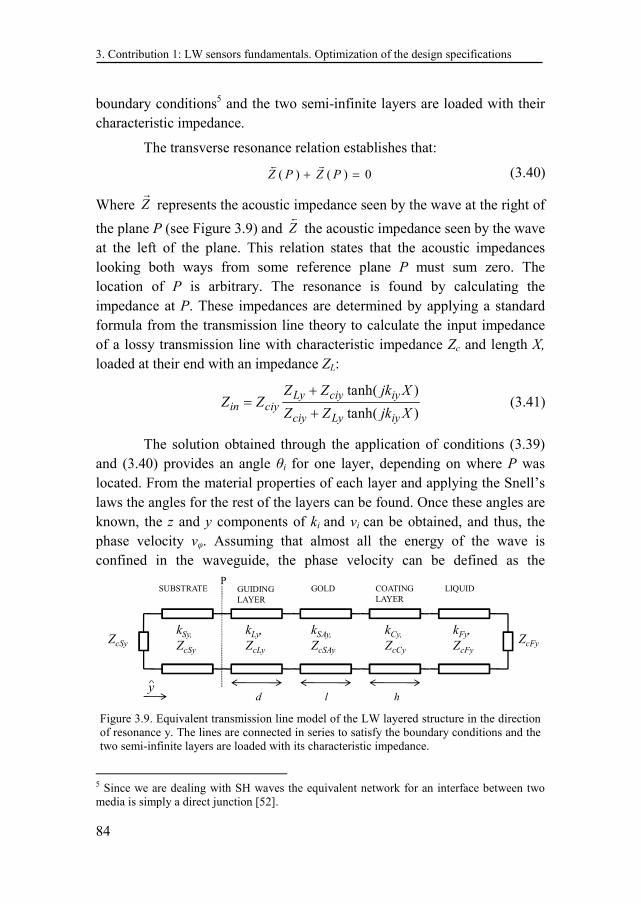
3. Contribution 1: LW sensors fundamentals. Optimization of the design specifications
84
boundary conditions5 and the two semi-infinite layers are loaded with their characteristic impedance.
The transverse resonance relation establishes that:
( ) ( ) 0Z P Z P+ =
(3.40)
Where Z
represents the acoustic impedance seen by the wave at the right of
the plane P (see Figure 3.9) and Z
the acoustic impedance seen by the wave at the left of the plane. This relation states that the acoustic impedances looking both ways from some reference plane P must sum zero. The location of P is arbitrary. The resonance is found by calculating the impedance at P. These impedances are determined by applying a standard formula from the transmission line theory to calculate the input impedance of a lossy transmission line with characteristic impedance Zc and length X, loaded at their end with an impedance ZL:
tanh( )
tanh( )Ly ciy iy
in ciyciy Ly iy
Z Z jk XZ Z
Z Z jk X
+=
+ (3.41)
The solution obtained through the application of conditions (3.39) and (3.40) provides an angle θi for one layer, depending on where P was located. From the material properties of each layer and applying the Snell’s laws the angles for the rest of the layers can be found. Once these angles are known, the z and y components of ki and vi can be obtained, and thus, the phase velocity vφ. Assuming that almost all the energy of the wave is confined in the waveguide, the phase velocity can be defined as the
5 Since we are dealing with SH waves the equivalent network for an interface between two media is simply a direct junction [52].
Figure 3.9. Equivalent transmission line model of the LW layered structure in the direction of resonance y. The lines are connected in series to satisfy the boundary conditions and the two semi-infinite layers are loaded with its characteristic impedance.
kSy,
ZcSy
P
ZcSy
SUBSTRATE GUIDING LAYER
GOLD COATING LAYER
LIQUID
d l h
ZcFy
kLy,
ZcLy
kSAy,
ZcSAy
kCy,
ZcCy
kFy,
ZcFy
y
María Isabel Rocha Gaso
85
wavefront velocity of the acoustic wave propagating in the guiding layer, which in this case propagates in the z direction. In lossless materials, kiz and kiy are real numbers and therefore vφ is given by:
1
sin sin sinL L
Lz L L L L L
vv
k kϕ
ω ω µθ θ θ ρ
= = = = (3.42)
where it can be appreciated that knowing the material properties which compose the LW devices, the value of vφ, can be determined.
When the material has losses, kiz and kiy are complex numbers with real and imaginary parts, and then the attenuation coefficients appear:
( ) ( )ˆ ˆˆ ˆi iz iy iz iz iy iyk k z k y j z j yβ α β α= + = − + − (3.43)
In this case, the phase velocity is given by:
1
sin sin
1
sin
Lz Lz L L L
L
LL
L L
vk k
v
j
ϕω ω ω
β θ θ
ρθ
µ ωη
= = = =ℜ ℜ
ℜ
=
ℜ +
(3.44)
On the other hand, the attenuation of the Love Wave, αLW, is considered to happen mostly in the propagation direction z, since in the resonance direction, y, a stationary wave takes place. Therefore:
sin
sinsin
LW Lz Lz L L
L LL
L L L
k k
v j
α α θ
θ ρθ
µ ωη
= = −ℑ = −ℑ
= −ℑ = −ℑ
+
(3.45)
Thus, following this procedure it is possible to obtain the phase velocity and attenuation of a LW propagating in a layer. Nevertheless, to complete this, it is necessary to know the material properties of all the layers which integrate the LW device. However, when the device is used as a sensor, and in particular in biosensor applications, the coating layer properties are unknown parameters. Thus, quantifying the variations suffered by the mechanical and geometric layer properties over the sensing layer when measuring vφ through some electrical parameters is what is really interesting when sensing.
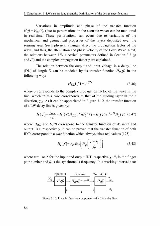
3. Contribution 1: LW sensors fundamentals. Optimization of the design specifications
86
Variations in amplitude and phase of the transfer function H(f) = Vout/Vin (due to perturbations in the acoustic wave) can be monitored in real-time. These perturbations can occur due to variations of the mechanical and geometrical properties of the layers deposited over the sensing area. Such physical changes affect the propagation factor of the wave, and thus, the attenuation and phase velocity of the Love Wave. Next, the relations between LW electrical parameters defined in Section 3.3 (φ and IL) and the complex propagation factor γ are explained.
The relation between the output and input voltage in a delay line (DL) of length D can be modeled by its transfer function HDL(f) in the following way:
( ) DDLH f e
γ−= (3.46)
where γ corresponds to the complex propagation factor of the wave in the line, which in this case corresponds to that of the guiding layer in the z direction, γLz. As it can be appreciated in Figure 3.10, the transfer function of a LW delay line is given by:
( ) 1 2 1 2( ) ( ) ( ) ( ) ( )Lz DoutDL
in
VH f H f H f H f H f e H f
V
γ−= = = (3.47)
where H1(f) and H2(f) correspond to the transfer function of de input and output IDT, respectively. It can be proven that the transfer function of both IDTs correspond to a sinc function which always takes real values [175]:
( ) 0
0sinci m p
f fH f A N
f
−=
(3.48)
where m=1 or 2 for the input and output IDT, respectively, Np is the finger pair number and f0 is the synchronous frequency. In a working interval near
Figure 3.10. Transfer function components of a LW delay line.
H2(f)Vin Vout
Input IDT Output IDT
H1(f) HDL(f)= e-γD
D
Spacing
z
María Isabel Rocha Gaso
87
to f0, Hm(f)≈Am
6 and the phase of Hm(f) is 0°. Thus:
( ) ( )
( )1 2 1 2
out in
Lz LzLz
j jout out out
in in in
j DD
V V VH f e e
V V V
A A e A A e
ϕ ϕ ϕ
α βγ
−
− +−
= = =
= ⋅ ⋅ = ⋅ ⋅
(3.49)
Hence, the phase-shift and IL are given by:
10 10 1 2
10 1 2 10
20 log 20 log
20 log 20 log
Lz Dout
in
Lz
Lz
VIL A A e
V
A A D e
D
α
α
ϕ β
−= ⋅ = ⋅ ⋅ ⋅
= ⋅ ⋅ − ⋅ ⋅
= −
(3.50)
Therefore, the increment in IL/D and φ/D from a non perturbed state γLz0 to a perturbed state γLz1 is the following:
( )1 0
1 0
20 logLz Lz
Lz Lz
ILe
D
D
α α
ϕβ β
∆= − ⋅
∆= −
(3.51)
The last set of equations provides a relation between the experimental data (IL, φ) and the physical parameters of the layers, which appears through αLz and βLz. The extraction of the layers physical parameters is a major problem. Assuming that the physical properties of the substrate, guiding layer, gold and fluid medium are known and that these properties do not change during the sensing process, which can be the case in biosensing, still the parameters of the coating layer are not known. In the case of QCM technology, the wave propagation direction in the QCM coincides with the resonant direction. Therefore, for low frequency QCM applications it is possible to assume that the biochemical interaction is translated to simple mass changes, since it is reasonable to assume that the thickness of the coating layer is acoustically thin. This simplifies enormously the parameters extraction. However, in LW sensors, this assumption is not valid, and then, the two experimental data obtained in LW devices (Eq. (3.51)) are not enough to extract the unknown parameters of the coating. This, together
6 Am may be considered equal to 1 for a uniformly apodized IDT.
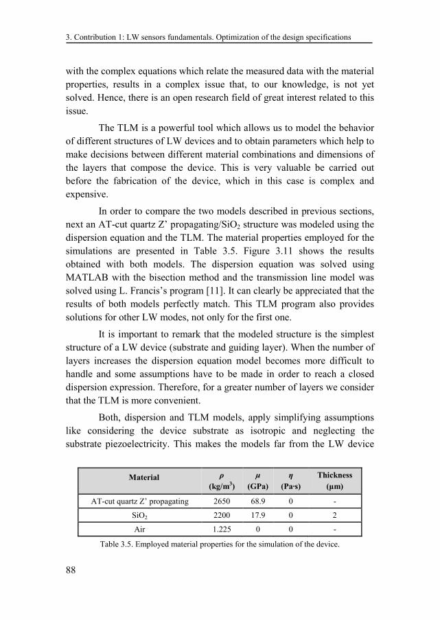
3. Contribution 1: LW sensors fundamentals. Optimization of the design specifications
88
with the complex equations which relate the measured data with the material properties, results in a complex issue that, to our knowledge, is not yet solved. Hence, there is an open research field of great interest related to this issue.
The TLM is a powerful tool which allows us to model the behavior of different structures of LW devices and to obtain parameters which help to make decisions between different material combinations and dimensions of the layers that compose the device. This is very valuable be carried out before the fabrication of the device, which in this case is complex and expensive.
In order to compare the two models described in previous sections, next an AT-cut quartz Z’ propagating/SiO2 structure was modeled using the dispersion equation and the TLM. The material properties employed for the simulations are presented in Table 3.5. Figure 3.11 shows the results obtained with both models. The dispersion equation was solved using MATLAB with the bisection method and the transmission line model was solved using L. Francis’s program [11]. It can clearly be appreciated that the results of both models perfectly match. This TLM program also provides solutions for other LW modes, not only for the first one.
It is important to remark that the modeled structure is the simplest structure of a LW device (substrate and guiding layer). When the number of layers increases the dispersion equation model becomes more difficult to handle and some assumptions have to be made in order to reach a closed dispersion expression. Therefore, for a greater number of layers we consider that the TLM is more convenient.
Both, dispersion and TLM models, apply simplifying assumptions like considering the device substrate as isotropic and neglecting the substrate piezoelectricity. This makes the models far from the LW device
Material ρ
(kg/m3)
µ
(GPa)
η
(Pa·s)
Thickness
(µm)
AT-cut quartz Z’ propagating 2650 68.9 0 -
SiO2 2200 17.9 0 2
Air 1.225 0 0 -
Table 3.5. Employed material properties for the simulation of the device.
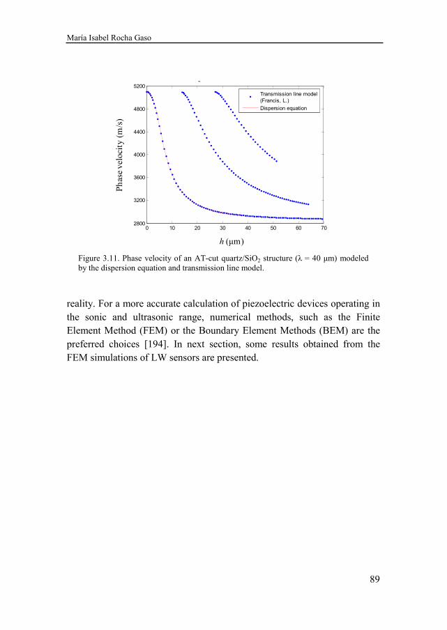
María Isabel Rocha Gaso
89
reality. For a more accurate calculation of piezoelectric devices operating in the sonic and ultrasonic range, numerical methods, such as the Finite Element Method (FEM) or the Boundary Element Methods (BEM) are the preferred choices [194]. In next section, some results obtained from the FEM simulations of LW sensors are presented.
Figure 3.11. Phase velocity of an AT-cut quartz/SiO2 structure (λ = 40 µm) modeled by the dispersion equation and transmission line model.
0 10 20 30 40 50 60 702800
3200
3600
4000
4400
4800
5200
h (µm)
2
Transmission line model
(Francis, L.)
Dispersion equation
h (µm)
Ph
ase
velo
city
(m
/s)
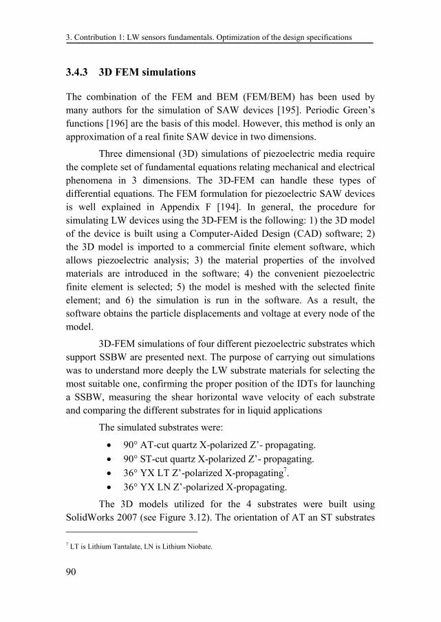
3. Contribution 1: LW sensors fundamentals. Optimization of the design specifications
90
3.4.3 3D FEM simulations
The combination of the FEM and BEM (FEM/BEM) has been used by many authors for the simulation of SAW devices [195]. Periodic Green’s functions [196] are the basis of this model. However, this method is only an approximation of a real finite SAW device in two dimensions.
Three dimensional (3D) simulations of piezoelectric media require the complete set of fundamental equations relating mechanical and electrical phenomena in 3 dimensions. The 3D-FEM can handle these types of differential equations. The FEM formulation for piezoelectric SAW devices is well explained in Appendix F [194]. In general, the procedure for simulating LW devices using the 3D-FEM is the following: 1) the 3D model of the device is built using a Computer-Aided Design (CAD) software; 2) the 3D model is imported to a commercial finite element software, which allows piezoelectric analysis; 3) the material properties of the involved materials are introduced in the software; 4) the convenient piezoelectric finite element is selected; 5) the model is meshed with the selected finite element; and 6) the simulation is run in the software. As a result, the software obtains the particle displacements and voltage at every node of the model.
3D-FEM simulations of four different piezoelectric substrates which support SSBW are presented next. The purpose of carrying out simulations was to understand more deeply the LW substrate materials for selecting the most suitable one, confirming the proper position of the IDTs for launching a SSBW, measuring the shear horizontal wave velocity of each substrate and comparing the different substrates for in liquid applications
The simulated substrates were:
• 90° AT-cut quartz X-polarized Z’- propagating.
• 90° ST-cut quartz X-polarized Z’- propagating.
• 36° YX LT Z’-polarized X-propagating7.
• 36° YX LN Z’-polarized X-propagating.
The 3D models utilized for the 4 substrates were built using SolidWorks 2007 (see Figure 3.12). The orientation of AT an ST substrates
7 LT is Lithium Tantalate, LN is Lithium Niobate.
María Isabel Rocha Gaso
91
is the same and the orientation of LT and LN substrates is the same. Later, these models were imported from ANSYS v. 11, a commercial finite element software, which allows piezoelectric analysis. The substrates' material properties were introduced in this software (such properties can be found in Appendix D). The hexahedral element Solid 5 with 4 degrees of
freedom (dof) was selected for the model. Three dofs were used for particle displacement in the x, y and z directions and the fourth one for voltage (ux, uy, uz and V respectively).
The meshing of the model was created in such a way that the highest density of nodes was concentrated at the device surface having a constant element length and a width of 5 µm. A variable element depth was set by 10 divisions in the substrate depth with an ANSYS spacing ratio of 100. A total number of 100 800 and 102 720 elements, for AT-ST and LT-LN models respectively, were generated once the model was entirely meshed in ANSYS vs. 11 (Figure 3.13).
The two-port delay line structure consisted of two finger pairs in each port. The IDTs were defined on the piezoelectric substrate as massless electrodes so that the second order effects of the electrodes can be ignored to simplify the computation [197,198]. The distribution of the IDTs is shown in Figure 3.14. The input IDT port comprises fingers A, B, C and D, while the output IDT port comprises fingers E, F, G and H. Fingers A, C, E, G were grounded and the excitation of the structure was provided by a sine function of 10 V peak-to-peak (V(t) = 5·sin(2πf·t) [V]) applied to fingers B
Figure 3.12. (Left) 3D models for 90° AT-cut quartz and 90° ST-cut quartz. (Right) 3D models for 36° YX LiTaO3 and 36° YX LiNbO3 (units in micrometers).
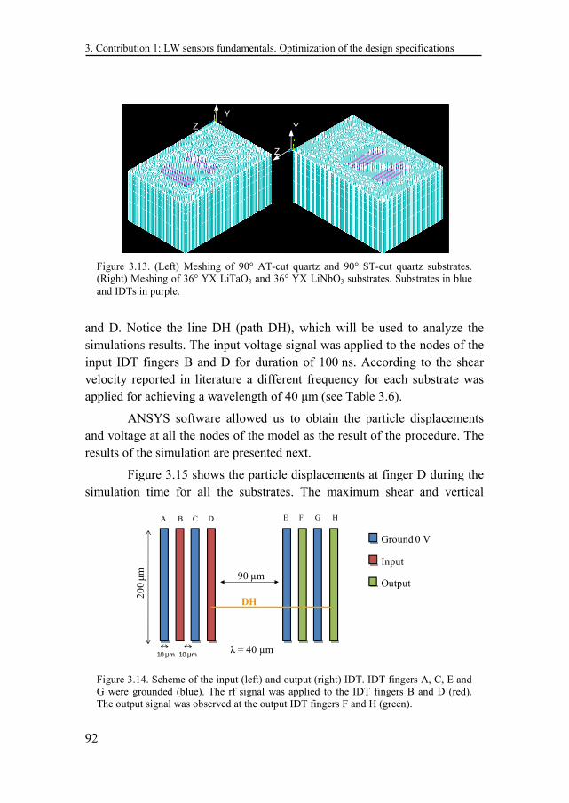
3. Contribution 1: LW sensors fundamentals. Optimization of the design specifications
92
and D. Notice the line DH (path DH), which will be used to analyze the simulations results. The input voltage signal was applied to the nodes of the input IDT fingers B and D for duration of 100 ns. According to the shear velocity reported in literature a different frequency for each substrate was applied for achieving a wavelength of 40 µm (see Table 3.6).
ANSYS software allowed us to obtain the particle displacements and voltage at all the nodes of the model as the result of the procedure. The results of the simulation are presented next.
Figure 3.15 shows the particle displacements at finger D during the simulation time for all the substrates. The maximum shear and vertical
Figure 3.13. (Left) Meshing of 90° AT-cut quartz and 90° ST-cut quartz substrates. (Right) Meshing of 36° YX LiTaO3 and 36° YX LiNbO3 substrates. Substrates in blue and IDTs in purple.
Y
Z
Y
Z
Figure 3.14. Scheme of the input (left) and output (right) IDT. IDT fingers A, C, E and G were grounded (blue). The rf signal was applied to the IDT fingers B and D (red). The output signal was observed at the output IDT fingers F and H (green).
A F HE
Output
Input
Ground 0 V
90 µm
10 µm 10 µmλ = 40 µm
GC DB
200
µm
DH
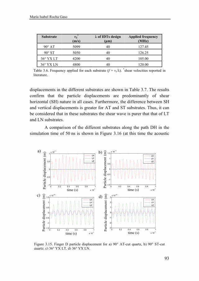
María Isabel Rocha Gaso
93
displacements in the different substrates are shown in Table 3.7. The results confirm that the particle displacements are predominantly of shear horizontal (SH) nature in all cases. Furthermore, the difference between SH and vertical displacements is greater for AT and ST substrates. Thus, it can be considered that in these substrates the shear wave is purer that that of LT and LN substrates.
A comparison of the different substrates along the path DH in the simulation time of 50 ns is shown in Figure 3.16 (at this time the acoustic
Substrate vS*
(m/s) λ of IDTs design
(µm) Applied frequency
(MHz)
90° AT 5099 40 127.45
90° ST 5050 40 126.25
36° YX LT 4200 40 105.00
36° YX LN 4800 40 120.00
Table 3.6. Frequency applied for each substrate (f = vs/λ). *shear velocities reported in literature.
Figure 3.15. Finger D particle displacement for a) 90° AT-cut quartz, b) 90° ST-cut quartz, c) 36° YX LT, d) 36° YX LN.
0 0.2 0.4 0.6 0.8 1
x 10-7
-1
-0.5
0
0.5
1x 10
-11
time (s)
UX
UY
UZ
0 0.2 0.4 0.6 0.8 1
x 10-7
-1.5
-1
-0.5
0
0.5
1
1.5x 10
-11
time (s)
Part
icle
dis
plac
emen
t (m
) UX
UY
UZ
0 0.2 0.4 0.6 0.8 1
x 10-7
-3
-2
-1
0
1
2
3x 10
-10
time (s)
UX
UY
UZ
0 0.2 0.4 0.6 0.8 1
x 10-7
-1.5
-1
-0.5
0
0.5
1
1.5x 10
-10
time (s)
UX
UY
UZ
c)
b)
d)
a)
Par
ticle
dis
plac
emen
t (m
)P
artic
le d
ispl
acem
ent
(m)
Par
ticle
dis
plac
emen
t (m
)P
artic
le d
ispl
acem
ent
(m)
time (s)
time (s)time (s)
time (s)
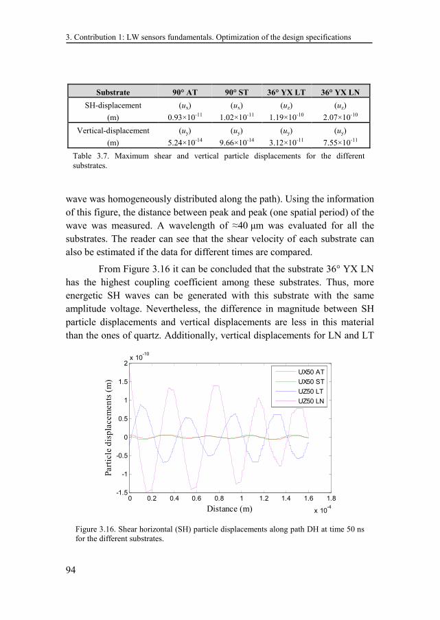
3. Contribution 1: LW sensors fundamentals. Optimization of the design specifications
94
wave was homogeneously distributed along the path). Using the information of this figure, the distance between peak and peak (one spatial period) of the wave was measured. A wavelength of ≈40 µm was evaluated for all the substrates. The reader can see that the shear velocity of each substrate can also be estimated if the data for different times are compared.
From Figure 3.16 it can be concluded that the substrate 36° YX LN has the highest coupling coefficient among these substrates. Thus, more energetic SH waves can be generated with this substrate with the same amplitude voltage. Nevertheless, the difference in magnitude between SH particle displacements and vertical displacements are less in this material than the ones of quartz. Additionally, vertical displacements for LN and LT
Figure 3.16. Shear horizontal (SH) particle displacements along path DH at time 50 ns for the different substrates.
0 0.2 0.4 0.6 0.8 1 1.2 1.4 1.6 1.8
x 10-4
-1.5
-1
-0.5
0
0.5
1
1.5
2x 10
-10
Distance (m)
Part
icle
dis
plac
emen
ts (
m)
UX50 AT
UX50 ST
UZ50 LT
UZ50 LN
Substrate 90° AT 90° ST 36° YX LT 36° YX LN
SH-displacement
(m)
(ux)
0.93×10⁻¹¹
(ux)
1.02×10⁻¹¹
(uz)
1.19×10⁻¹⁰
(uz)
2.07×10⁻¹⁰
Vertical-displacement
(m)
(uy)
5.24×10⁻¹⁴
(uy)
9.66×10⁻¹⁴
(uy)
3.12×10⁻¹¹
(uy)
7.55×10⁻¹¹
Table 3.7. Maximum shear and vertical particle displacements for the different substrates.
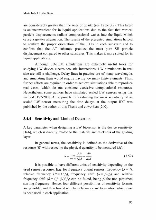
María Isabel Rocha Gaso
95
are considerably greater than the ones of quartz (see Table 3.7). This latest is an inconvenient for in liquid applications due to the fact that vertical particle displacements radiate compressional waves into the liquid which cause a greater attenuation. The results of the presented simulations helped to confirm the proper orientation of the IDTs in each substrate and to confirm that the AT substrate produce the most pure SH particle displacement compared to other substrates. This makes it more suited for in liquid applications.
Although 3D-FEM simulations are extremely useful tools for studying LW device electro-acoustic interactions, LW simulations in real size are still a challenge. Delay lines in practice are of many wavelengths and simulating them would require having too many finite elements. Thus, further efforts are required in order to achieve simulations able to reproduce real cases, which do not consume excessive computational resources. Nevertheless, some authors have simulated scaled LW sensors using this method [197-200]. An approach for evaluating the mass sensitivity of an scaled LW sensor measuring the time delays at the output IDT was published by the author of this Thesis and coworkers [200].
3.4.4 Sensitivity and Limit of Detection
A key parameter when designing a LW biosensor is the device sensitivity [166], which is directly related to the material and thickness of the guiding layer.
In general terms, the sensitivity is defined as the derivative of the response (R) with respect to the physical quantity to be measured (M):
0
limM
R dRS
M dM∆ →
∆= =
∆ (3.52)
It is possible to have different units of sensitivity depending on the used sensor response. E.g. for frequency output sensors, frequency (R = f), relative frequency (R = f / f0), frequency shift (R = f - f0) and relative frequency shift (R = ( f - f0 )/ f0) can be found, being f0 the non perturbed starting frequency. Hence, four different possibilities of sensitivity formats are possible, and therefore it is extremely important to mention which case is been used in each application.
3. Contribution 1: LW sensors fundamentals. Optimization of the design specifications
96
The sensitivity of LW sensors gives the correlation between measured electric signals delivered by the sensor and a perturbing event which takes place on the sensing area of the sensor. A high sensitivity relates a strong signal variation with a small perturbation [11]. Depending on the employed electronic configuration, the electrical signal measured in LW devices can be: operating frequency, amplitude (or insertion loss), and phase. From the frequency and phase, and using the theoretical models, the phase velocity and group velocity can be obtained (see Sections 3.4.1 and 3.4.2).
When the sensor response R is the phase velocity, and the perturbing event which takes place on the sensing area is a variation of the surface mass density of the coating σ (σ = h·ρC), the velocity mass sensitivity Sσ
v of a LW device at a constant frequency, f, is given by [11,201]:
0
1v
f
vS
v
ϕσ
ϕ σ
∂=
∂ (3.53)
where vφ0 is the unperturbed phase velocity and vφ is the phase velocity after a surface mass change. Hence, Sσ
v has units of m2/kg. In Eq. (3.53) partial derivatives have been considered as the phase velocity depends on several variables.
In sensor applications the phase velocity shift must be obtained from the experimental values of phase or frequency shifts. For the closed loop configuration, where the experimentally measured quantity is the frequency, the frequency mass sensitivity Sσ
f is defined as:
0
1f dfS
f dσ σ
= (3.54)
Jakoby and Vellekoop [201] noticed that the sensitivity measured by frequency changes in an oscillator (Eq. (3.54)) differs from the estimated velocity mass sensitivity (Eq. (3.53)) by a factor vg/vφ (Sσ
f = (vg/vφ)Sσ
v), since Love modes are dispersive. Thus, typically Sσ
v is a 10% higher than Sσf.
For the open loop configuration, where the experimentally measured quantity is the phase, the phase sensitivity also called gravimetric
sensitivity, Sσφ, in absence of interferences is defined as:
María Isabel Rocha Gaso
97
1 v
Lz
dS S
k D d
ϕσ σ
ϕσ
= = (3.55)
where D is the distance between input and output IDT (see Figure 3.4a) and kLz is the wavenumber of the Love mode (see Eq. (3.45)), therefore kLzD is the unperturbed phase φ0.
In those applications where a coating layer in contact with a liquid is deposited over the sensing area, such is the case of biosensors, both changes in the surface mass density ∆σ and in the mass viscosity ∆(ρCηC)1/2 of the coating occur, due to the biochemical interaction between the coating and the liquid medium In this case, the sensitivity can be modeled by the four components matrix shown in Eq. (3.56) [15]. The matrix components relate shifts of surface mass density ∆σ and mass viscosity ∆(ρη)1/2 to shifts of electrical phase ∆φ and signal attenuation ∆IL. Notice that Sφ,σ is not the same than Sσ
φ in Eq. (3.55). The relation between them can be found in reference [11].
, ,
, ,
C C
C C
C CIL IL
S S
IL S S
ϕ σ ϕ ρ η
σ ρ η
σϕ
ρ η
∆ ∆ = ∆ ∆
(3.56)
The theoretical mass sensitivity for LW devices with two layers (substrate plus guiding layer), in which a small perturbation is produced at the guiding layer, can be determined by means of the perturbation theory [193] from the phase velocity according to [190]:
12sin( ) cos( ) cos ( )11 Ly Ly Lyv S
L Ly L Sy
k d k d k dS
d k d k dσ
ρρ ρ
−
= − + +
(3.57)
where kLy is the wavenumber in the guiding layer (Eq. (3.2)) and kSy is the wavenumber in the substrate (Eq. (3.58)).
2 2
2 2Sy
S
kv vϕ
ω ω= − (3.58)
The minus sing in Eq. (3.57) indicates that the phase velocity of the perturbed event due to an increment in the surface mass density is less than the unperturbed phase velocity (∆vφ = vφ- vφ0). The phase velocity in Eq. (3.58) can be obtained from the dispersion equation (Eq. (3.1)) or the
3. Contribution 1: LW sensors fundamentals. Optimization of the design specifications
98
transmission line model (Eq. (3.44)). Once the phase velocity is known, the mass sensitivity curve can be obtained using Eq. (3.57).
Generally, the high sensitivity of microacoustic sensors is closely related to the fact that they show a high temperature stability (low TCF) and a large signal-to-noise ratio, which, in turn yields low LOD and a high resolution of the sensor [166].
Sensitivity, together with the LOD, are important characteristic of acoustic biosensors which allow us to know the suitability of a technology for a given application. The LOD depends on the sensitivity of the device, but also on its characterization system. The LOD can be directly derived from the ratio between the noise in the measured electrical signal Nf and the sensitivity of the device. For instance, in a closed loop configuration, this noise Nf is the root mean square (RMS) value of the frequency measured over a given period of time in stable and constant conditions [11]. It is usually recommended to measure a signal variation higher than 3 times the noise level in order to conclude from an effective variation [202]. From this recommendation, it comes out that the LOD is given by [11,203]:
0
3LOD f
r f
N
S fσ
σ⋅
= ∆ =⋅
(3.59)
where fo is the operating frequency. In this way, we can also define the LOD for phase measurements as [142]:
0
3LOD
N
S
ϕϕσ ϕ
⋅=
⋅ (3.60)
The LOD can be improved, for example, by minimizing the influence of temperature on the sensor response [166]. The stability with respect to temperature can be achieved by implementing temperature control in the biosensor system and choosing materials of low TCF, as seen in Section 3.2.1. In next section a study to determine the effect of temperature on AT-cut and ST-cut quartz substrates is presented.
María Isabel Rocha Gaso
99
3.5 Studies to define other design specifications
In this section some studies are presented which allowed us to establish the design specifications of the LW sensor that will be developed for the Thesis. Such studies allowed us to select the more suitable substrate, guiding layer material and the optimal wavelength. Other studied aspects were the use of the optimal guiding layer thickness and reflectors.
In next Section 3.5.1 the temperature stability of ST and AT-cut quartz was proven experimentally. From this study, the most suited substrate was confirmed. Later, in Section 3.5.2, the sensitivity of two different guiding layer materials is analyzed. This study helped us to make a decision regarding the guiding layer material to be employed in the final design. In addition in this section the optimal synchronous frequency of LW devices with different wavelength were explored theoretically. In Section 3.5.3 some experiments were set in order to decide whether to use reflectors in the final LW sensor design. Last, the issue of LW sensors’ packaging and flow cells is briefly addressed.
3.5.1 Temperature effect: Selection of the substrate material
Measurements of temperature stability of two crystal cuts (Z’ propagating ST and AT- quartz cut) were carried out. The purpose of this study was to confirm that the AT-cut substrate material is more thermally stable and thus, better for biosensing applications than the ST-cut.
SH-SAW devices with wavelength of 12 µm, no reflectors and double-finger IDTs with 200 nm thickness were used8. Measurements were performed using an Agilent N5242A premier-performance Network Analyzer (NA) while the temperature of a chuck plate, where the wafers were placed, was varied. The NA was calibrated with 401 points in a frequency range of 400 MHz–440 MHz, being these conditions the same for both AT and ST-cut quartz measurements. Temperature was varied from room temperature to 85°C. The measurements’ results are presented in
8 For further information regarding the IDT pattering process the reader can refere to Chapter 4 of this manuscript.
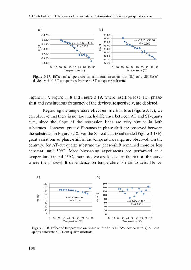
3. Contribution 1: LW sensors fundamentals. Optimization of the design specifications
100
Figure 3.17, Figure 3.18 and Figure 3.19, where insertion loss (IL), phase-shift and synchronous frequency of the devices, respectively, are depicted.
Regarding the temperature effect on insertion loss (Figure 3.17), we can observe that there is not too much difference between AT and ST-quartz cuts, since the slope of the regression lines are very similar in both substrates. However, great differences in phase-shift are observed between the substrates in Figure 3.18. For the ST-cut quartz substrate (Figure 3.18b), great variations of phase-shift in the temperature range are observed. On the contrary, for AT-cut quartz substrate the phase-shift remained more or less constant until 50ºC. Most biosensing experiments are performed at a temperature around 25ºC, therefore, we are located in the part of the curve where the phase-shift dependence on temperature is near to zero. Hence,
Figure 3.17. Effect of temperature on minimum insertion loss (IL) of a SH-SAW device with a) AT-cut quartz substrate b) ST-cut quartz substrate.
y = -0.014x - 38.06
R² = 0.959
-39.40
-39.20
-39.00
-38.80
-38.60
-38.40
-38.20
0 10 20 30 40 50 60 70 80 90
IL (d
B)
Temperature (°C)
a)
y = -0.015x - 35.76
R² = 0.962
-37.40
-37.20
-37.00
-36.80
-36.60
-36.40
-36.20
-36.00
-35.80
0 10 20 30 40 50 60 70 80 90
IL(d
B)
Temperature (°C)
b)
Figure 3.18. Effect of temperature on phase-shift of a SH-SAW device with a) AT-cut quartz substrate b) ST-cut quartz substrate.
y = -0.178x + 132.6
R² = 0.250
0
20
40
60
80
100
120
140
160
0 10 20 30 40 50 60 70 80 90
Ph
ase
(°)
Temperature (°C)
a)
y = 0.046x + 117.7
R² = 0.003
0
20
40
60
80
100
120
140
160
0 10 20 30 40 50 60 70 80 90
Ph
ase
(°)
Temperature (°C)
b)
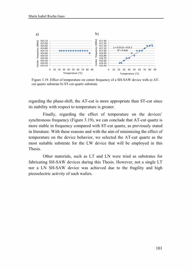
María Isabel Rocha Gaso
101
regarding the phase-shift, the AT-cut is more appropriate than ST-cut since its stability with respect to temperature is greater.
Finally, regarding the effect of temperature on the devices’ synchronous frequency (Figure 3.19), we can conclude that AT-cut quartz is more stable in frequency compared with ST-cut quartz, as previously stated in literature. With these reasons and with the aim of minimizing the effect of temperature on the device behavior, we selected the AT-cut quartz as the most suitable substrate for the LW device that will be employed in this Thesis.
Other materials, such as LT and LN were tried as substrates for fabricating SH-SAW devices during this Thesis. However, not a single LT nor a LN SH-SAW device was achieved due to the fragility and high piezoelectric activity of such wafers.
Figure 3.19. Effect of temperature on center frequency of a SH-SAW device with a) AT-cut quartz substrate b) ST-cut quartz substrate.
y = 0.012x + 416.2
R² = 0.956
416.40416.50416.60416.70416.80416.90417.00417.10417.20417.30417.40
0 10 20 30 40 50 60 70 80 90
Temperature (°C)
Ce
nte
r f
req
ue
ncy
(M
Hz)
b)
424.10424.20424.30424.40424.50424.60424.70424.80424.90425.00425.10
0 10 20 30 40 50 60 70 80 90
Temperature (°C)
Ce
nte
r f
req
ue
ncy
(M
Hz)
a)
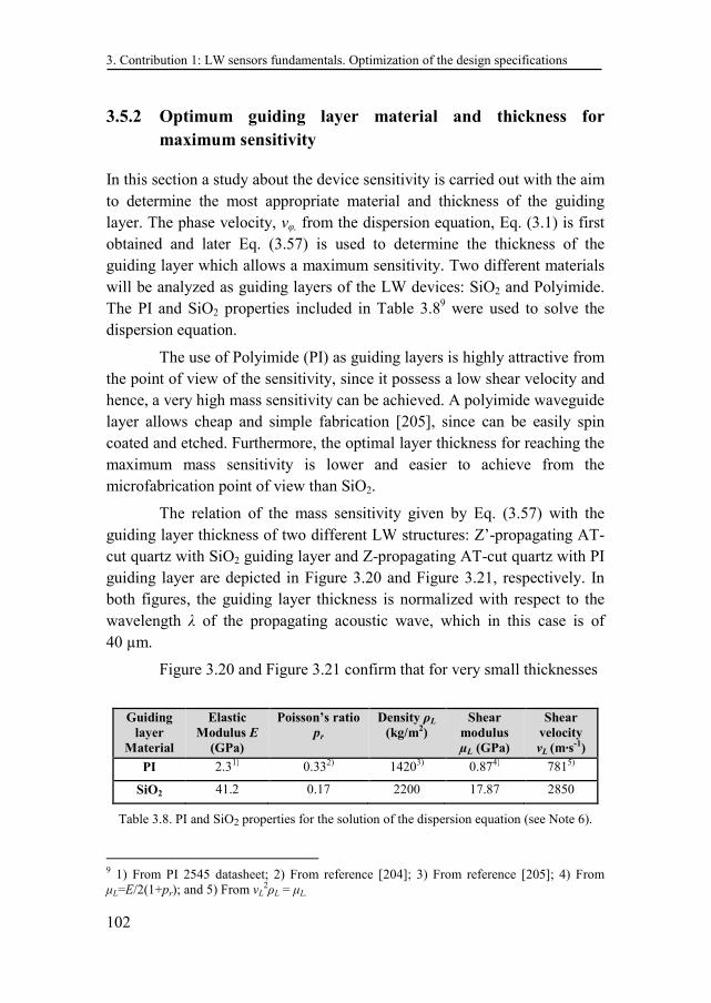
3. Contribution 1: LW sensors fundamentals. Optimization of the design specifications
102
3.5.2 Optimum guiding layer material and thickness for
maximum sensitivity
In this section a study about the device sensitivity is carried out with the aim to determine the most appropriate material and thickness of the guiding layer. The phase velocity, vφ, from the dispersion equation, Eq. (3.1) is first obtained and later Eq. (3.57) is used to determine the thickness of the guiding layer which allows a maximum sensitivity. Two different materials will be analyzed as guiding layers of the LW devices: SiO2 and Polyimide. The PI and SiO2 properties included in Table 3.89 were used to solve the dispersion equation.
The use of Polyimide (PI) as guiding layers is highly attractive from the point of view of the sensitivity, since it possess a low shear velocity and hence, a very high mass sensitivity can be achieved. A polyimide waveguide layer allows cheap and simple fabrication [205], since can be easily spin coated and etched. Furthermore, the optimal layer thickness for reaching the maximum mass sensitivity is lower and easier to achieve from the microfabrication point of view than SiO2.
The relation of the mass sensitivity given by Eq. (3.57) with the guiding layer thickness of two different LW structures: Z’-propagating AT-cut quartz with SiO2 guiding layer and Z-propagating AT-cut quartz with PI guiding layer are depicted in Figure 3.20 and Figure 3.21, respectively. In both figures, the guiding layer thickness is normalized with respect to the wavelength λ of the propagating acoustic wave, which in this case is of 40 µm.
Figure 3.20 and Figure 3.21 confirm that for very small thicknesses
9 1) From PI 2545 datasheet; 2) From reference [204]; 3) From reference [205]; 4) From µL=E/2(1+pr); and 5) From vL
2ρL = µL.
Guiding layer
Material
Elastic Modulus E
(GPa)
Poisson’s ratio pr
Density ρL
(kg/m2) Shear
modulus µL (GPa)
Shear velocity vL (m·s-1)
PI 2.31) 0.332) 14203) 0.874) 7815)
SiO2 41.2 0.17 2200 17.87 2850
Table 3.8. PI and SiO2 properties for the solution of the dispersion equation (see Note 6).
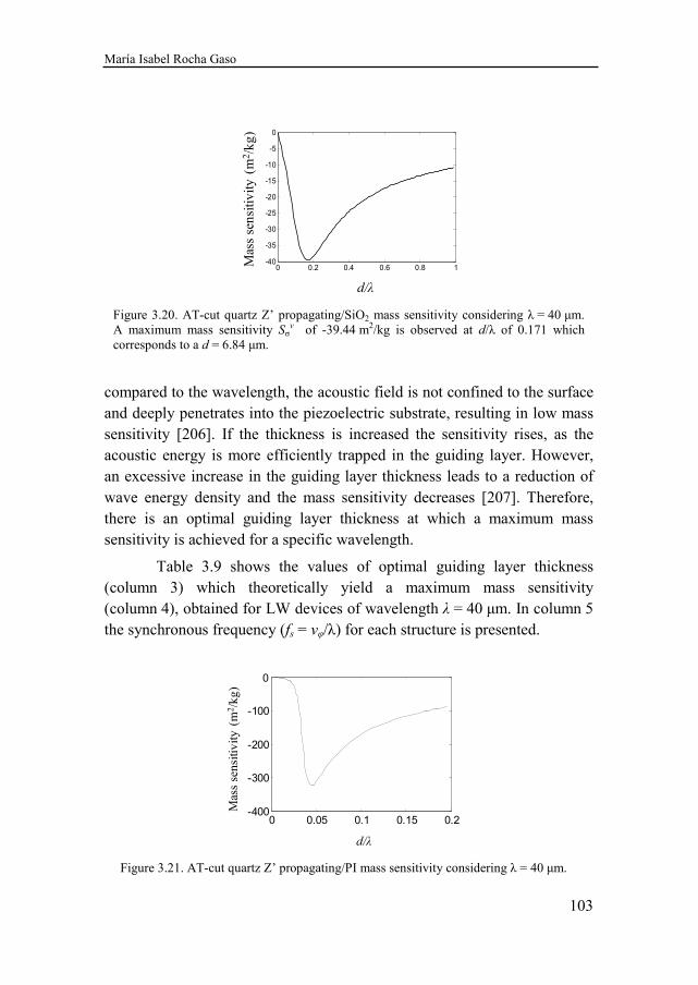
María Isabel Rocha Gaso
103
compared to the wavelength, the acoustic field is not confined to the surface and deeply penetrates into the piezoelectric substrate, resulting in low mass sensitivity [206]. If the thickness is increased the sensitivity rises, as the acoustic energy is more efficiently trapped in the guiding layer. However, an excessive increase in the guiding layer thickness leads to a reduction of wave energy density and the mass sensitivity decreases [207]. Therefore, there is an optimal guiding layer thickness at which a maximum mass sensitivity is achieved for a specific wavelength.
Table 3.9 shows the values of optimal guiding layer thickness (column 3) which theoretically yield a maximum mass sensitivity (column 4), obtained for LW devices of wavelength λ = 40 µm. In column 5 the synchronous frequency (fs = vφ/λ) for each structure is presented.
Figure 3.21. AT-cut quartz Z’ propagating/PI mass sensitivity considering λ = 40 µm.
0 0.05 0.1 0.15 0.2-400
-300
-200
-100
0
d/λd/λ
Mas
s se
nsiti
vity
(m
2 /kg
)
Figure 3.20. AT-cut quartz Z’ propagating/SiO2 mass sensitivity considering λ = 40 µm. A maximum mass sensitivity Sσ
v
of -39.44 m2/kg is observed at d/λ of 0.171 which
corresponds to a d = 6.84 µm.
d/λ
0 0.2 0.4 0.6 0.8 1-40
-35
-30
-25
-20
-15
-10
-5
0
λd/λ
Mas
s se
nsiti
vity
(m
2 /kg
)
3. Contribution 1: LW sensors fundamentals. Optimization of the design specifications
104
From Table 3.9 it can be appreciated that a much higher mass sensitivity can be achieved with a PI guiding layer. The theoretical values obtained for PI seemed very attractive, therefore, such LW device was fabricated. The Insertion Loss (IL) of this fabricated device measured with an Agilent Network Analyzer N524A is shown in Figure 3.22. In the figure, the device response with PI thickness of 1 um and gold sensing area of 50 nm can be appreciated. An IL of up to -40 dB is observed. Therefore, a higher attenuation is produced when placing a gold sensing area in the surface due to the high acoustic damping (losses) of the PI polymer. Thus, we confirmed what was earlier stated by Turton et al. [205]; the theoretical optimum thickness for maximum sensitivity when using PI cannot be approached due to large insertion losses at that layer thickness. For this reason, PI was not selected as the guiding layer for the final LW of this
Structure λ
(µm) Optimal layer thickness (µm)
Corresponding mass sensitivity (m2/kg)
fs (MHz)
90° AT/SiO2 40 6.84 -39.4 103.50
90° AT/PI 40 1.76 -324.2 110.25
Table 3.9. Optimal layer thickness for two different LW structures with λ of 40 µm.
Figure 3.22. 90° AT/PI/Au LW structure with λ = 40 µm and 1 µm PI thickness.
121 122 123 124 125 126 127 128-75
-70
-65
-60
-55
-50
-45
-40
-35
Frequency (MHz)
IL (
dB
)
AT/PI/Au
María Isabel Rocha Gaso
105
Thesis. On the contrary, with SiO2 guiding layer (Figure 3.23) a less attenuated device frequency response was obtained.
Finally, to end with this section and considering that the selected substrate material is Z’-propagating AT-cut quartz and the selected guiding layer is SiO2, the optimal guiding layer thickness, operating frequency and maximum mass sensitivity for such structure and different wavelengths were determined using the TLM program developed by L. Francis [11]. The results are shown in Table 3.10. AT-quartz cut and ST-cut quartz SH-SAW devices with these wavelengths were implemented. We did not achieve good devices with wavelengths greater than 40 µm. With these results and
Figure 3.23. 90° AT/SiO2/Au LW structure with λ = 40 µm and 2 µm SiO2 thickness.
118 120 122 124 126 128-80
-70
-60
-50
-40
-30
-20
-10
Frequency (MHz)
IL (
dB
)
AT/SiO2/Au
Wavelength (µm)
Optimal guiding layer thickness (µm)
Sσv
(m2/kg) fs (MHz)
100 17.10 -15.77 41.40
60 10.26 -26.29 69.00
40 6.84 -39.44 103.50
20 3.42 -78.87 207.00
12 2.05 -131.45 345.00
6 1.03 -262.89 690.00
Table 3.10. Optimal waveguide thickness and operating frequency for a maximum mass sensitivity Sσ
v of a AT-cut quartz/SiO2 LW structure for different wavelengths.
3. Contribution 1: LW sensors fundamentals. Optimization of the design specifications
106
the values of Table 3.10 we made a decision regarding the wavelength for the final device. We required an operating frequency around 100 MHz, in order to compare the LW device with HFF-QCM devices developed at our research group. Therefore, a wavelength of 40 µm was selected. Hence, an optimal guiding layer of around 6 µm was pursued.
3.5.3 Reflectors for enhancing the device response
The use of reflectors for enhancing LW sensor response in a bandwidth around the synchronous frequency has been proposed by some authors [147,174]. With the purpose of evaluating the use of these grating structures in the LW sensor final design, different kind of reflectors on two-port LW sensors acoustic response were implemented in this Thesis.
The typical metallic gratings, described by Hashimoto [174], are open-circuited (OC), short-circuited (SC) and positive and negative reflection (PNR) (see Figure 3.24).
The use of metallic gratings on piezoelectric substrates causes electrical reflection in addition to mechanical reflection [174]. Due to these reflections, the propagation of the SAW is perturbed. In addition, the charge induced on the metal strips regenerates the SAWs. Due to this, the reflection characteristics of the structure are very dependent upon the electrical connection among the strips [174]. In the OC grating, each strip is electrically isolated. The SC grating has every strip connected electrically in parallel and the PNR grating is the combination of both gratings. According to Hashimoto’s works, this latest configuration offers a larger reflection coefficient than OC or SC gratings [174].
LW devices with Z’ propagating ST-cut quartz substrate, aluminum
Figure 3.24. Typical metallic grating.
a) OC grating b) SC grating c) PNR grating
María Isabel Rocha Gaso
107
double-finger IDTs with λ = 40 µm (5 µm wide of each strip), 0.6 µm SiO2 guiding layer and 200 finger of 5 µm wide reflectors, in the three configurations (OC, SC and PNR), were fabricated. The use of a resin as an absorbing material at the end of each device was required for the measurements (Figure 3.25), for without this resin unwanted reflections and cross taking of the devices were produced.
A probe station was used to carry out on-wafer measurements of the fabricated devices. The S-parameters of the devices were observed and recorded using an Agilent N5242A Network Analyzer. The IL and phase-shift of these devices were compared the different reflectors' structures. In Figure 3.26 the frequency response of the devices with different reflectors is shown. Figure 3.27 presents a zoom of the frequency responses’ central part (around the synchronous frequency).
The SC reflector configuration presents the lowest IL among the implemented grating. However, the use of SC reflectors, in our case, did not produce a significant improvement in the IL, contrarily to what is stated in literature. Thus, after these results, it was decided not to use the reflectors gratings for the final LW sensor design, since it was not clearly seen a significant improvement in the acoustic response of the sensors with these gratings.
As a future work, it would be extremely interesting to study the effect of the reflectors on the sensors’ mass sensitivity. For this study, one possibility is to perform an experimental calibration of the sensors’ mass sensitivity with different type of reflectors. Some mass sensitivity calibration techniques are described by Francis, L. [11].
Figure 3.25. ST-quartz wafer with fabricated devices. The orange resin, placed at the ends of the devices, acts as absorbing material.
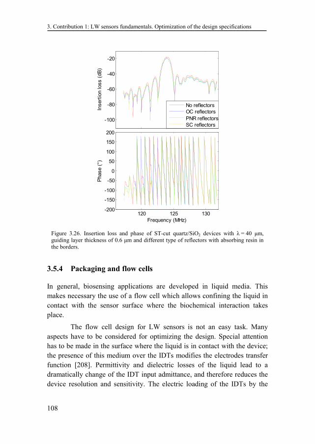
3. Contribution 1: LW sensors fundamentals. Optimization of the design specifications
108
3.5.4 Packaging and flow cells
In general, biosensing applications are developed in liquid media. This makes necessary the use of a flow cell which allows confining the liquid in contact with the sensor surface where the biochemical interaction takes place.
The flow cell design for LW sensors is not an easy task. Many aspects have to be considered for optimizing the design. Special attention has to be made in the surface where the liquid is in contact with the device; the presence of this medium over the IDTs modifies the electrodes transfer function [208]. Permittivity and dielectric losses of the liquid lead to a dramatically change of the IDT input admittance, and therefore reduces the device resolution and sensitivity. The electric loading of the IDTs by the
Figure 3.26. Insertion loss and phase of ST-cut quartz/SiO2 devices with λ = 40 µm, guiding layer thickness of 0.6 µm and different type of reflectors with absorbing resin in the borders.
-100
-80
-60
-40
-20
Insert
ion loss (
dB
)No reflectors
OC reflectors
PNR reflectors
SC reflectors
120 125 130-200
-150
-100
-50
0
50
100
150
200
Frequency (MHz)
Phase (
°)
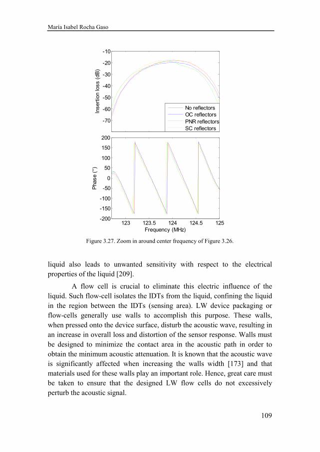
María Isabel Rocha Gaso
109
liquid also leads to unwanted sensitivity with respect to the electrical properties of the liquid [209].
A flow cell is crucial to eliminate this electric influence of the liquid. Such flow-cell isolates the IDTs from the liquid, confining the liquid in the region between the IDTs (sensing area). LW device packaging or flow-cells generally use walls to accomplish this purpose. These walls, when pressed onto the device surface, disturb the acoustic wave, resulting in an increase in overall loss and distortion of the sensor response. Walls must be designed to minimize the contact area in the acoustic path in order to obtain the minimum acoustic attenuation. It is known that the acoustic wave is significantly affected when increasing the walls width [173] and that materials used for these walls play an important role. Hence, great care must be taken to ensure that the designed LW flow cells do not excessively perturb the acoustic signal.
Figure 3.27. Zoom in around center frequency of Figure 3.26.
123 123.5 124 124.5 125-80
-70
-60
-50
-40
-30
-20
-10
Frequency (MHz)
Insert
ion loss (
dB
)
No reflectors
OC reflectors
PNR reflectors
SC reflectors
123 123.5 124 124.5 125-200
-150
-100
-50
0
50
100
150
200
Frequency (MHz)
Phase (
°)
3. Contribution 1: LW sensors fundamentals. Optimization of the design specifications
110
On the other hand, the flow cell design, together with other factors, such as the flow through system also influence the binding efficiency and the course of binding kinetics of the agents involved in the biosensing application interaction process. This results in possible variations of the true results [61]. Therefore, in biosensing experiments, the flow-through cell design and the whole fluidic system (syringes, valves, flow velocity, etc.) is a critical point.
Flow cells are usually constructed with an inlet at one side, an outlet at the other and the channels facing the sensor. In most cases, with the aim of confining the liquid in the sensing area, a rubber seal is used for sealing. Moreover, for LW devices, additional absorbers made with rubber materials at the ends of the IDTs are recommended to improve the signal response, minimizing the unwanted acoustic reflections from the device borders.
Recently, some researchers have explored different possibilities to achieve the packaging of LW sensors for fluidic applications [173,210] and other authors have being exploring different LW flow-cell approaches [149,211,212]. Nevertheless, further improvements for LW biosensors flow cells can be achieved, since it is an entirely new field and the development trends moves towards smaller flow cells which allows the use of less chemicals. For instance, investigation on the materials used for creating flow cells, packaging, and flow patterns in microfluidic channels [61] would enhance LW performance and move them faster to the lab-on-a-chip arena.
The design and development of a flow-through cell for the LW sensors employed in this work is one of the contributions of this Thesis. The flow cell design affects the device design due to the necessary electric connections between the cell and the device. This is the reason why it is important to have in mind the design of the LW devices together with the design of the flow cell. The implementation and results of the LW flow-through cell are presented in Chapter 5 of this manuscript.
3.6 Chapter conclusion
The most important result of this chapter is the determination of the appropriate materials and dimensions of the different components that will form the LW sensor structure employed in this Thesis (substrate, guiding
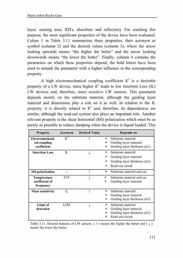
María Isabel Rocha Gaso
111
layer, sensing area, IDTs, absorbers and reflectors). For reaching this purpose, the most significant properties of the device have been evaluated. Colum 1 in Table 3.11 summarizes these properties, their acronym or symbol (column 2) and the desired values (column 3), where the arrow looking upwards means “the higher the better” and the arrow looking downwards means “the lower the better”. Finally, column 4 contains the parameters on which these properties depend; the bold letters have been used to remark the parameter with a higher influence in the corresponding property.
A high electromechanical coupling coefficient K2 is a desirable
property of a LW device, since higher K2 leads to low Insertion Loss (IL) LW devices and, therefore, more sensitive LW sensors. This parameter depends mostly on the substrate material, although the guiding layer material and dimensions play a role on it as well. In relation to the IL property, it is directly related to K
2 and, therefore, its dependences are similar, although the read-out system also plays an important role. Another relevant property is the shear horizontal (SH) polarization which must be as purely as possible to reduce damping when the device is liquid loaded. This
Property Acronym Desired Value Depends on
Electromechani-cal coupling coefficient
K2 ↑ Substrate material Guiding layer material Guiding layer thickness (d/λ)
Insertion Loss IL ↓ Substrate material Guiding layer material Guiding layer thickness (d/λ) Read out circuit
SH-polarization -- ↑ Substrate material and cut
Temperature coefficient of
frequency
TCF ↓ Substrate material and cut Guiding layer material
Mass sensitivity Sσ ↑ Substrate material Guiding layer material Guiding layer thickness (d/λ)
Limit of detection
LOD ↓ Substrate material Guiding layer material Guiding layer thickness (d/λ) Read out circuit
Table 3.11. Desired features of LW sensors. ( ↑ ) means the higher the better and ( ↓ ) means the lower the better.
3. Contribution 1: LW sensors fundamentals. Optimization of the design specifications
112
property is directly related to the substrate material and cut.
A deep review of the available literature, together with some studies carried out along this chapter about some of the previously mentioned properties, have allowed to conclude that the best LW sensor configuration for the research objectives of this thesis is an AT-cut quartz Z’ propagating substrate, with double-finger aluminum IDTs, SiO2 guiding layer and gold sensing area.
AT-cut substrate was chosen mainly for two reasons: 1) its high thermal stability allows to improve the LOD which was one of the general objectives of the project in which this thesis is framed; and 2) because it generates purely SH polarized waves, which is the best option when working in-liquid media applications, as it is the case of biosensors.
Aluminum IDTs were chosen for their ability to resist corrosion, low cost and for their demonstrated suitability for this purpose. A double-electrode IDTs with 5 µm spacing was chosen for a wavelength of 40 µm, which fixes the operating frequency around 100 MHz for the LW structure with the selected materials. The LW device operating frequency was chosen around this range so a more appropriate comparison with the available HFF-QCM sensors can be performed (second general objective of this Thesis). The frequency of HFF-QCMs is around 100-150 MHz.
In relation to the guiding layer, the two criteria taken into account for the selection of the material and dimensions were the achievement of the maximum mass sensitivity and a suitable IL. LW devices with thicker guiding layers show larger insertion loss while loaded with water [11] and from the microfabrication point of view thicker guiding layers are more difficult to etch and handle, therefore, a trade-off between optimal mass sensitivity and devices insertion loss performance has to be made. In this sense, although Polyimide (PI) provides a great mass sensitivity, its high acoustic damping (losses) prevents it to be used in the final biosensor applications. Therefore, SiO2 guiding layer was chosen due to its low acoustic damping and because it is widely use in standard microelectronics processes. Modeling results for the LW structure AT-cut quartz/SiO2 shows that the optimal guiding layer thickness for maximum sensitivity is 6.84 µm (see Table 3.10). However, some restrictions in the microfabrication
María Isabel Rocha Gaso
113
process, which are explained in next chapter, prevented us to reach this thickness.
The gold sensing area was selected because most of the biochemical protocols (immobilization techniques) in biosensors applications are performed over this material.
When it comes to the reflectors gratings, it was decided not to use them for the final LW sensor design, since not a significant improvement in the frequency response of the sensors was appreciated with these gratings. The use of an absorbing material at the end of each device was incorporated in the final design.
Although the most important result of this chapter is the definition of the final device structure, other conclusions must be remarked. In this sense, with regard to the modeling methods section it is worth to mention that for those applications with a high number of layers, as in the case of biosensors, the use of the TLM is more convenient than the dispersion equation, since it is a very structured and intuitive model where the addition of an extra layer does not make the procedure more complex. Nevertheless, both, dispersion and TLM models, applied simplifying assumptions like considering the device substrate as isotropic and neglecting the substrate piezoelectricity. This makes the models far from the LW device reality. For a more accurate calculation of piezoelectric devices operating in the sonic and ultrasonic range, numerical methods, such as the Finite Element Method (FEM) are the preferred choices. But, even if 3D-FEM simulations are extremely useful tools for studying LW device electro-acoustic interactions, LW simulations in real dimensions are still a challenge and consume excessive computational resources.
In relation to the measurement techniques, the characterization system used in this thesis is based upon an open loop configuration. The system, which will be described in Chapter 5, is essentially the same as that used for the characterization of HFF-QCM sensors with the aim to preserve the measurement conditions as similar as possible in both technologies. In this way, the comparison will be more useful and reliable.
In addition, in this chapter it has been remarked the need to develop an ad-hoc and optimized flow-through cell for LW devices. Such design establishes certain aspects of the final sensor design, like the location and
3. Contribution 1: LW sensors fundamentals. Optimization of the design specifications
114
shape of the electric contacts between the device and the cell (as it will be seen in Chapters 4 and 5).
Once the main aspects of the components of the LW device structure were clarified, the next step was the fabrication of the device. In next chapter the fabrication process of the defined LW device is presented.
María Isabel Rocha Gaso
115
4. Contribution 2: Fabrication and
characterization of the LW sensor
4.1 Introduction
The studies carried out in Chapter 3 of this Thesis led us to the best LW sensor configuration for the application and experiment setup we pursue. A LW sensor with AT-cut quartz substrate, SiO2 guiding layer, λ = 40 µm and gold sensing layer was determined to be fabricated. In this chapter the final devices and each of the steps of the process followed to achieve their fabrication are described. The electric characterization of the final fabricated LW sensors is also presented.
The fabrication procedure and electric characterization described in this chapter were carried out at the Institute for Information and Communication Technologies, Electronics and Applied Mathematics (ICTEAM) at the Université catholique de Louvain (UCL), in Belgium. This institute is equipped with two main state-of-the-art technological platforms: WINFAB and WELCOME, which were used to fabricate and characterize the LW sensors, respectively.
WINFAB stands for Wallonia Infrastructure NanoFABrication and is a 1000 m2 class 10 microelectronics cleanroom established for flexible research and development and for technological convergence. It results from 40 years of investigation at UCL in silicon technologies and is currently one of the European excellence platform in nanoelectronics and one of the 17 major R&D infrastructures in Belgium. The current research activities in WINFAB are micronic fully-depleted Silicon-On-Insulator CMOS process,
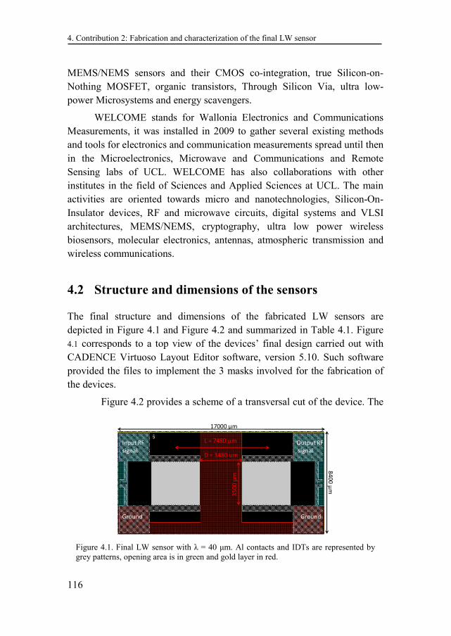
4. Contribution 2: Fabrication and characterization of the final LW sensor
116
MEMS/NEMS sensors and their CMOS co-integration, true Silicon-on-Nothing MOSFET, organic transistors, Through Silicon Via, ultra low-power Microsystems and energy scavengers.
WELCOME stands for Wallonia Electronics and Communications Measurements, it was installed in 2009 to gather several existing methods and tools for electronics and communication measurements spread until then in the Microelectronics, Microwave and Communications and Remote Sensing labs of UCL. WELCOME has also collaborations with other institutes in the field of Sciences and Applied Sciences at UCL. The main activities are oriented towards micro and nanotechnologies, Silicon-On- Insulator devices, RF and microwave circuits, digital systems and VLSI architectures, MEMS/NEMS, cryptography, ultra low power wireless biosensors, molecular electronics, antennas, atmospheric transmission and wireless communications.
4.2 Structure and dimensions of the sensors
The final structure and dimensions of the fabricated LW sensors are depicted in Figure 4.1 and Figure 4.2 and summarized in Table 4.1. Figure
4.1 corresponds to a top view of the devices’ final design carried out with CADENCE Virtuoso Layout Editor software, version 5.10. Such software provided the files to implement the 3 masks involved for the fabrication of the devices.
Figure 4.2 provides a scheme of a transversal cut of the device. The
Figure 4.1. Final LW sensor with λ = 40 µm. Al contacts and IDTs are represented by grey patterns, opening area is in green and gold layer in red.
17000 µm
84
00
µm
D = 3480 um
35
00
µm
Input RF
signal
Output RF
signal
Ground Ground
L = 7480 µm
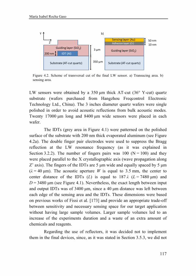
María Isabel Rocha Gaso
117
LW sensors were obtained by a 350 µm thick AT-cut (36° Y-cut) quartz substrate (wafers purchased from Hangzhou Freqcontrol Electronic Technology Ltd., China). The 3 inches diameter quartz wafers were single polished in order to avoid acoustic reflections from bulk acoustic modes. Twenty 17000 µm long and 8400 µm wide sensors were placed in each wafer.
The IDTs (grey area in Figure 4.1) were patterned on the polished surface of the substrate with 200 nm thick evaporated aluminum (see Figure 4.2a). The double finger pair electrodes were used to suppress the Bragg reflection at the LW resonance frequency (as it was explained in Section 3.2.2). The number of fingers pairs was 100 (N = 100) and they were placed parallel to the X crystallographic axis (wave propagation along Z’ axis). The fingers of the IDTs are 5 µm wide and equally spaced by 5 µm (λ = 40 µm). The acoustic aperture W is equal to 3.5 mm, the center to center distance of the IDTs (L) is equal to 187 λ (L = 7480 µm) and D = 3480 µm (see Figure 4.1). Nevertheless, the exact length between input and output IDTs was of 3400 µm, since a 40 µm distance was left between each edge of the sensing area and the IDTs. These dimensions were based on previous works of Fissi et al. [173] and provide an appropriate trade-off between sensitivity and necessary sensing space for our target application without having large sample volumes. Larger sample volumes led to an increase of the experiments duration and a waste of an extra amount of chemicals and reagents.
Regarding the use of reflectors, it was decided not to implement them in the final devices, since, as it was stated in Section 3.5.3, we did not
Figure 4.2. Scheme of transversal cut of the final LW sensor. a) Transucing area. b) sensing area.
IDT (Al)
Substrate (AT-cut quartz)
200 nm
350 μm
3 μmGuiding layer (SiO2)
Substrate (AT-cut quartz)
10 nm
50 nmAdhesion layer (Cr)
Sensing layer (Au)
Guiding layer (SiO2)
b)
Z’
Y
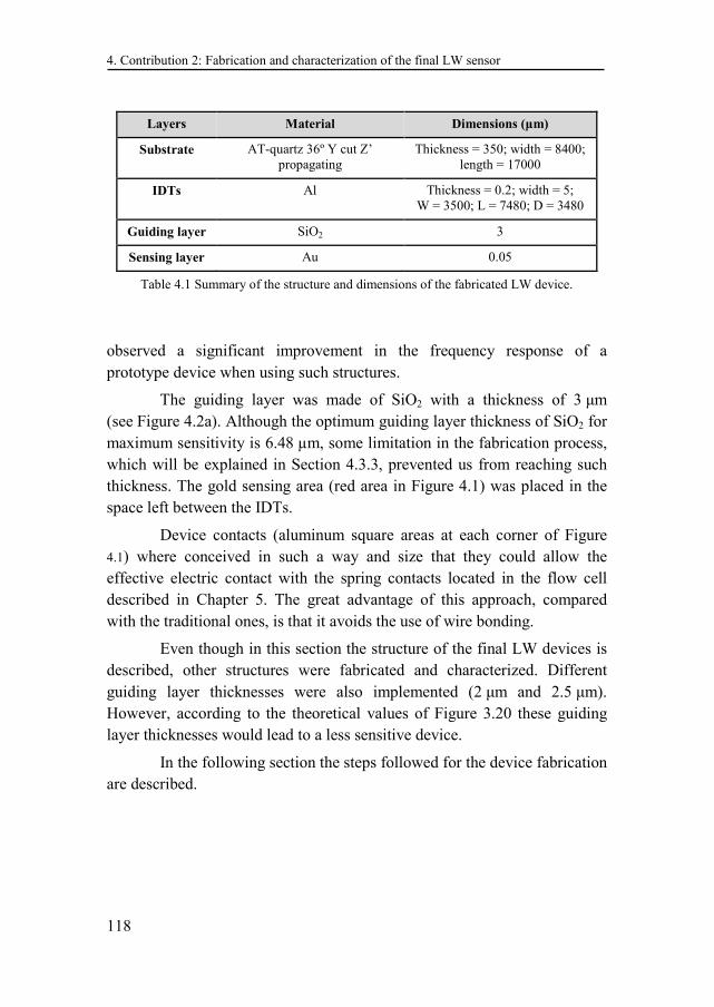
4. Contribution 2: Fabrication and characterization of the final LW sensor
118
observed a significant improvement in the frequency response of a prototype device when using such structures.
The guiding layer was made of SiO2 with a thickness of 3 µm (see Figure 4.2a). Although the optimum guiding layer thickness of SiO2 for maximum sensitivity is 6.48 µm, some limitation in the fabrication process, which will be explained in Section 4.3.3, prevented us from reaching such thickness. The gold sensing area (red area in Figure 4.1) was placed in the space left between the IDTs.
Device contacts (aluminum square areas at each corner of Figure
4.1) where conceived in such a way and size that they could allow the effective electric contact with the spring contacts located in the flow cell described in Chapter 5. The great advantage of this approach, compared with the traditional ones, is that it avoids the use of wire bonding.
Even though in this section the structure of the final LW devices is described, other structures were fabricated and characterized. Different guiding layer thicknesses were also implemented (2 µm and 2.5 µm). However, according to the theoretical values of Figure 3.20 these guiding layer thicknesses would lead to a less sensitive device.
In the following section the steps followed for the device fabrication are described.
Layers Material Dimensions (µm)
Substrate AT-quartz 36º Y cut Z’ propagating
Thickness = 350; width = 8400; length = 17000
IDTs Al Thickness = 0.2; width = 5; W = 3500; L = 7480; D = 3480
Guiding layer SiO2 3
Sensing layer Au 0.05
Table 4.1 Summary of the structure and dimensions of the fabricated LW device.
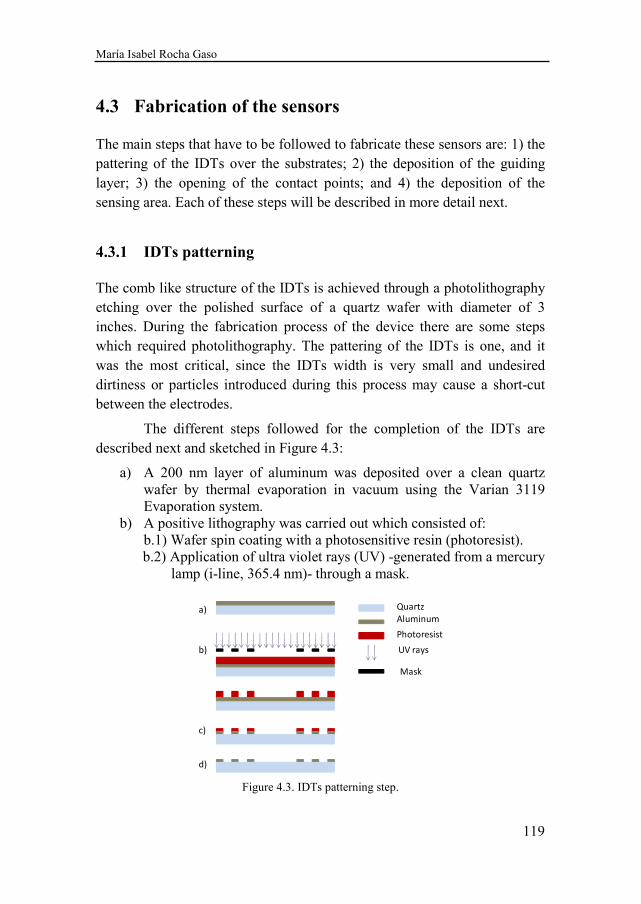
María Isabel Rocha Gaso
119
4.3 Fabrication of the sensors
The main steps that have to be followed to fabricate these sensors are: 1) the pattering of the IDTs over the substrates; 2) the deposition of the guiding layer; 3) the opening of the contact points; and 4) the deposition of the sensing area. Each of these steps will be described in more detail next.
4.3.1 IDTs patterning
The comb like structure of the IDTs is achieved through a photolithography etching over the polished surface of a quartz wafer with diameter of 3 inches. During the fabrication process of the device there are some steps which required photolithography. The pattering of the IDTs is one, and it was the most critical, since the IDTs width is very small and undesired dirtiness or particles introduced during this process may cause a short-cut between the electrodes.
The different steps followed for the completion of the IDTs are described next and sketched in Figure 4.3:
a) A 200 nm layer of aluminum was deposited over a clean quartz wafer by thermal evaporation in vacuum using the Varian 3119 Evaporation system.
b) A positive lithography was carried out which consisted of: b.1) Wafer spin coating with a photosensitive resin (photoresist). b.2) Application of ultra violet rays (UV) -generated from a mercury
lamp (i-line, 365.4 nm)- through a mask.
Figure 4.3. IDTs patterning step.
Quartz
Aluminuma)
b)
Photoresist
c)
d)
UV rays
Mask
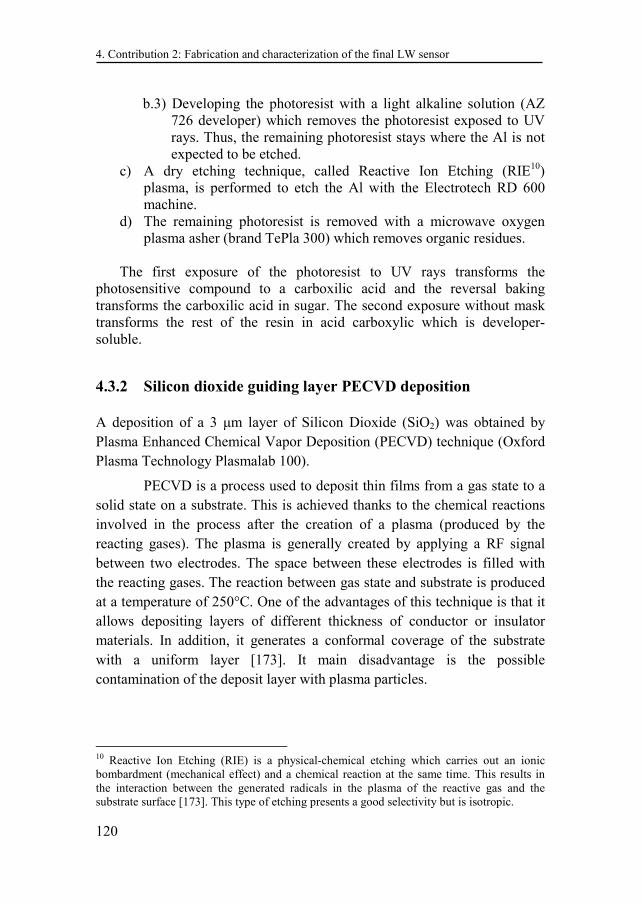
4. Contribution 2: Fabrication and characterization of the final LW sensor
120
b.3) Developing the photoresist with a light alkaline solution (AZ 726 developer) which removes the photoresist exposed to UV rays. Thus, the remaining photoresist stays where the Al is not expected to be etched.
c) A dry etching technique, called Reactive Ion Etching (RIE10) plasma, is performed to etch the Al with the Electrotech RD 600 machine.
d) The remaining photoresist is removed with a microwave oxygen plasma asher (brand TePla 300) which removes organic residues.
The first exposure of the photoresist to UV rays transforms the photosensitive compound to a carboxilic acid and the reversal baking transforms the carboxilic acid in sugar. The second exposure without mask transforms the rest of the resin in acid carboxylic which is developer-soluble.
4.3.2 Silicon dioxide guiding layer PECVD deposition
A deposition of a 3 µm layer of Silicon Dioxide (SiO2) was obtained by Plasma Enhanced Chemical Vapor Deposition (PECVD) technique (Oxford Plasma Technology Plasmalab 100).
PECVD is a process used to deposit thin films from a gas state to a solid state on a substrate. This is achieved thanks to the chemical reactions involved in the process after the creation of a plasma (produced by the reacting gases). The plasma is generally created by applying a RF signal between two electrodes. The space between these electrodes is filled with the reacting gases. The reaction between gas state and substrate is produced at a temperature of 250°C. One of the advantages of this technique is that it allows depositing layers of different thickness of conductor or insulator materials. In addition, it generates a conformal coverage of the substrate with a uniform layer [173]. It main disadvantage is the possible contamination of the deposit layer with plasma particles.
10 Reactive Ion Etching (RIE) is a physical-chemical etching which carries out an ionic bombardment (mechanical effect) and a chemical reaction at the same time. This results in the interaction between the generated radicals in the plasma of the reactive gas and the substrate surface [173]. This type of etching presents a good selectivity but is isotropic.
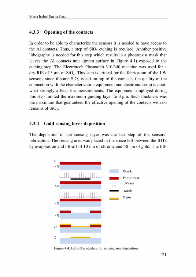
María Isabel Rocha Gaso
121
4.3.3 Opening of the contacts
In order to be able to characterize the sensors it is needed to have access to the Al contacts. Thus, a step of SiO2 etching is required. Another positive lithography is needed for this step which results in a photoresist mask that leaves the Al contacts area (green surface in Figure 4.1) exposed to the etching step. The Electrotech Plasmafab 310/340 machine was used for a dry RIE of 3 µm of SiO2. This step is critical for the fabrication of the LW sensors, since if some SiO2 is left on top of the contacts, the quality of the connection with the characterization equipment and electronic setup is poor, what strongly affects the measurements. The equipment employed during this step limited the maximum guiding layer to 3 µm. Such thickness was the maximum that guaranteed the effective opening of the contacts with no remains of SiO2.
4.3.4 Gold sensing layer deposition
The deposition of the sensing layer was the last step of the sensors’ fabrication. The sensing area was placed in the space left between the IDTs by evaporation and lift-off of 10 nm of chrome and 50 nm of gold. The lift-
Figure 4.4. Lift-off procedure for sensing area deposition.
Quartz
Photoresist
UV rays
a)
b)
c)
Mask
Cr/Au
a.1)
a.2)
a.3)
a.4)
4. Contribution 2: Fabrication and characterization of the final LW sensor
122
off process, which required a reversal lithography, is explain next and schematized in Figure 4.4.
a) A reversal lithography was carried out which consisted of: a.1) Wafer spin coating with a photoresist. a.2) Applying UV rays through a mask. a.3) A reversal baking and a second exposure to UV rays with no
mask. a.4) Developing of the photoresist with a developer, which removed
the photoresist that was not exposed to UV rays. Thus, the photoresist was removed where the Cr and Au were expected to remain.
b) A deposition of 10 nm of Cr and 50 nm of Au with the Vacotec double beam evaporator machine.
c) The remaining photoresist was removed with acetone and ultrasounds.
Figure 4.5a shows a quartz wafer with the final LW devices and Figure 4.5b shows the comparison of a single LW device with a one euro cent coin. Each wafer contained 20 LW sensors. To separate each of the sensors it was necessary to dice them with the high speed water lubricated dicing machine Tempress 602.
4.4 Characteristics of the fabricated sensors
In this section some features of the fabricated devices are summarized. First of all, some images of the sensing and transducing areas obtained with Atomic Force Microscopy (AFM) are shown. Later, the frequency response of the devices is presented: phase-shift and insertion loss. Finally, a study
Figure 4.5. a) Final LW sensors in quartz wafer. b) Size comparison of final LW sensor with a euro cent.
a) b)
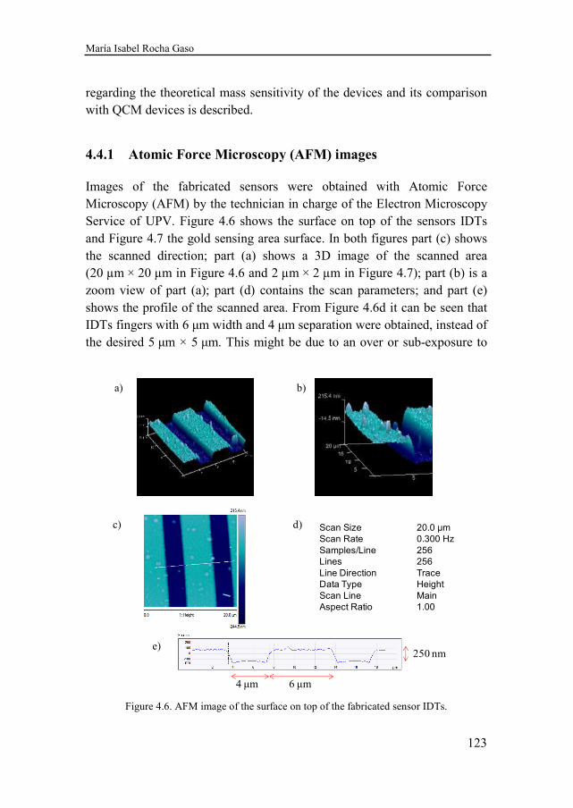
María Isabel Rocha Gaso
123
regarding the theoretical mass sensitivity of the devices and its comparison with QCM devices is described.
4.4.1 Atomic Force Microscopy (AFM) images
Images of the fabricated sensors were obtained with Atomic Force Microscopy (AFM) by the technician in charge of the Electron Microscopy Service of UPV. Figure 4.6 shows the surface on top of the sensors IDTs and Figure 4.7 the gold sensing area surface. In both figures part (c) shows the scanned direction; part (a) shows a 3D image of the scanned area (20 µm × 20 µm in Figure 4.6 and 2 µm × 2 µm in Figure 4.7); part (b) is a zoom view of part (a); part (d) contains the scan parameters; and part (e) shows the profile of the scanned area. From Figure 4.6d it can be seen that IDTs fingers with 6 µm width and 4 µm separation were obtained, instead of the desired 5 µm × 5 µm. This might be due to an over or sub-exposure to
Figure 4.6. AFM image of the surface on top of the fabricated sensor IDTs.
4 µm 6 µm
250 nm
a) b)
c)
e)
Scan Size 20.0 µm
Scan Rate 0.300 Hz
Samples/Line 256
Lines 256
Line Direction Trace
Data Type Height
Scan Line Main
Aspect Ratio 1.00
d)
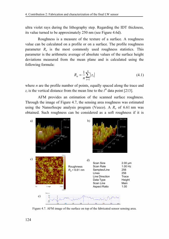
4. Contribution 2: Fabrication and characterization of the final LW sensor
124
ultra violet rays during the lithography step. Regarding the IDT thickness, its value turned to be approximately 250 nm (see Figure 4.6d).
Roughness is a measure of the texture of a surface. A roughness value can be calculated on a profile or on a surface. The profile roughness parameter Ra is the most commonly used roughness statistics. This parameter is the arithmetic average of absolute values of the surface height deviations measured from the mean plane and is calculated using the following formula:
1
1 n
a i
i
zRn =
= ∑ (4.1)
where n are the profile number of points, equally spaced along the trace and zi is the vertical distance from the mean line to the ith data point [213].
AFM provides an estimation of the scanned surface roughness. Through the image of Figure 4.7, the sensing area roughness was estimated using the NansoSocpe analysis program (Veeco). A Ra of 6.61 nm was obtained. Such roughness can be considered as a soft roughness if it is
Figure 4.7. AFM image of the surface on top of the fabricated sensor sensing area.
Roughness
Ra = 6.61 nm
a) b)
c)
e)
Scan Size 2.00 µm
Scan Rate 1.00 Hz
Samples/Line 256
Lines 256
Line Direction Trace
Data Type Height
Scan Line Main
Aspect Ratio 1.00
d)
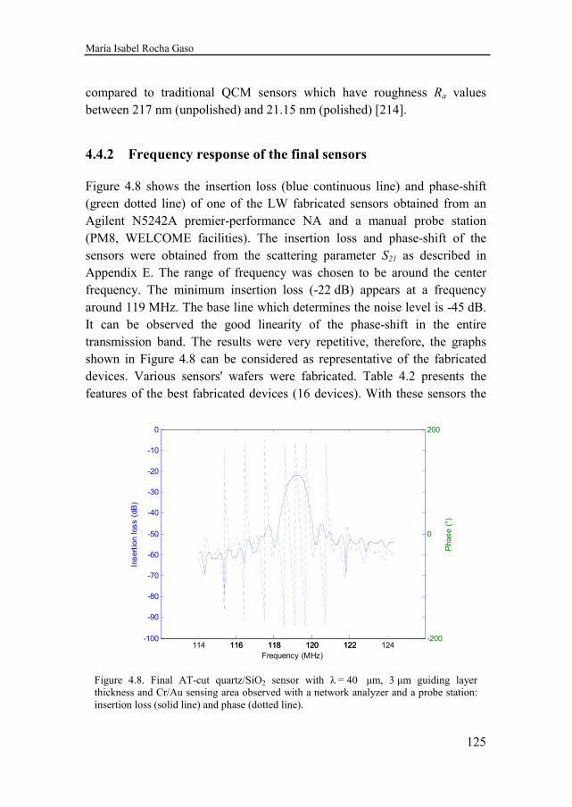
María Isabel Rocha Gaso
125
compared to traditional QCM sensors which have roughness Ra values between 217 nm (unpolished) and 21.15 nm (polished) [214].
4.4.2 Frequency response of the final sensors
Figure 4.8 shows the insertion loss (blue continuous line) and phase-shift (green dotted line) of one of the LW fabricated sensors obtained from an Agilent N5242A premier-performance NA and a manual probe station (PM8, WELCOME facilities). The insertion loss and phase-shift of the sensors were obtained from the scattering parameter S21 as described in Appendix E. The range of frequency was chosen to be around the center frequency. The minimum insertion loss (-22 dB) appears at a frequency around 119 MHz. The base line which determines the noise level is -45 dB. It can be observed the good linearity of the phase-shift in the entire transmission band. The results were very repetitive, therefore, the graphs shown in Figure 4.8 can be considered as representative of the fabricated devices. Various sensors' wafers were fabricated. Table 4.2 presents the features of the best fabricated devices (16 devices). With these sensors the
Figure 4.8. Final AT-cut quartz/SiO2 sensor with λ = 40 µm, 3 µm guiding layer thickness and Cr/Au sensing area observed with a network analyzer and a probe station: insertion loss (solid line) and phase (dotted line).
114 116 118 120 122 124-100
-90
-80
-70
-60
-50
-40
-30
-20
-10
0
Insert
ion loss (
dB
)
116 118 120 122-200
0
200
Frequency (MHz)
Phase (
°)
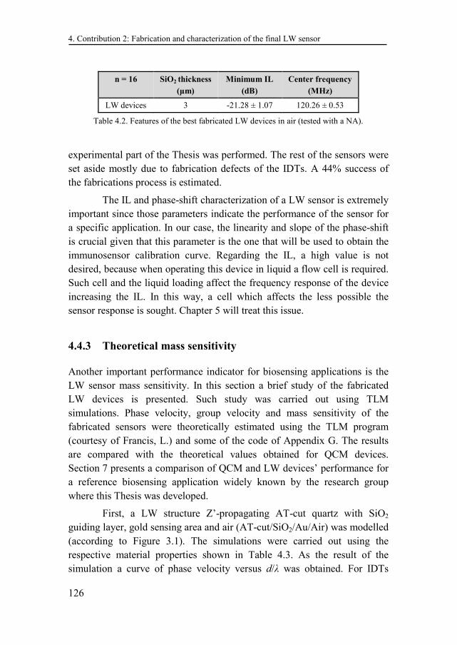
4. Contribution 2: Fabrication and characterization of the final LW sensor
126
experimental part of the Thesis was performed. The rest of the sensors were set aside mostly due to fabrication defects of the IDTs. A 44% success of the fabrications process is estimated.
The IL and phase-shift characterization of a LW sensor is extremely important since those parameters indicate the performance of the sensor for a specific application. In our case, the linearity and slope of the phase-shift is crucial given that this parameter is the one that will be used to obtain the immunosensor calibration curve. Regarding the IL, a high value is not desired, because when operating this device in liquid a flow cell is required. Such cell and the liquid loading affect the frequency response of the device increasing the IL. In this way, a cell which affects the less possible the sensor response is sought. Chapter 5 will treat this issue.
4.4.3 Theoretical mass sensitivity
Another important performance indicator for biosensing applications is the LW sensor mass sensitivity. In this section a brief study of the fabricated LW devices is presented. Such study was carried out using TLM simulations. Phase velocity, group velocity and mass sensitivity of the fabricated sensors were theoretically estimated using the TLM program (courtesy of Francis, L.) and some of the code of Appendix G. The results are compared with the theoretical values obtained for QCM devices. Section 7 presents a comparison of QCM and LW devices’ performance for a reference biosensing application widely known by the research group where this Thesis was developed.
First, a LW structure Z’-propagating AT-cut quartz with SiO2
guiding layer, gold sensing area and air (AT-cut/SiO2/Au/Air) was modelled (according to Figure 3.1). The simulations were carried out using the respective material properties shown in Table 4.3. As the result of the simulation a curve of phase velocity versus d/λ was obtained. For IDTs
n = 16 SiO2 thickness
(µm)
Minimum IL
(dB)
Center frequency
(MHz)
LW devices 3 -21.28 ± 1.07 120.26 ± 0.53
Table 4.2. Features of the best fabricated LW devices in air (tested with a NA).
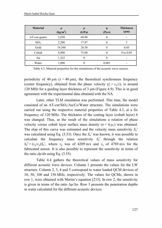
María Isabel Rocha Gaso
127
periodicity of 40 µm (λ = 40 µm), the theoretical synchronous frequency (center frequency), obtained from the phase velocity (fs = vφ/λ), is around 120 MHz for a guiding layer thickness of 3 µm (Figure 4.9). This is in good agreement with the experimental data obtained with the NA.
Later, other TLM simulation was performed. This time, the model consisted of an AT-cut/SiO2/Au/Co/Water structure. The simulations were carried out using the respective material properties of Table 4.3, at a fix frequency of 120 MHz. The thickness of the coating layer (cobalt layer) h was changed. Thus, as the result of the simulations a relation of phase velocity versus cobalt layer surface mass density (σ = h·ρC) was obtained. The slop of this curve was estimated and the velocity mass sensitivity Sσ
v was calculated using Eq. (3.53). Once the Sσ
v was known, it was possible to
calculate the frequency mass sensitivity Sσf through the relation
Sσf = (vg/vφ)Sσ
v, where vg was of 4209 m/s and vφ of 4789 m/s for the fabricated sensor. It is also possible to represent the sensitivity in terms of the ratio dφ/dσ using Eq. (3.55).
Table 4.4 gathers the theoretical values of mass sensitivity for different acoustic wave devices. Column 1 presents the values for the LW structure. Column 2, 3, 4 and 5 correspond to water loaded QCM devices of 10, 50, 100 and 150 MHz, respectively. The values for QCMs, shown in row 1, were obtained with Martin’s equation [215]. In row 2, the sensitivity is given in terms of the ratio ∆φ/∆σ. Row 3 presents the penetration depths in water calculated for the different acoustic devices.
Material ρ
(kg/m3)
µ
(GPa)
η
(Pa·s)
Thickness (µm)
AT-cut quartz 2,650 68.90 0 -
SiO2 2,200 17.87 0 3
Gold 19,300 28.50 0 0.05
Cobalt 8,900 75.00 0 0 to 0.05
Air 1.225 0 0 -
Water 1,000 0 0.001 -
Table 4.3. Material properties for the simulations of the acoustic wave sensors.
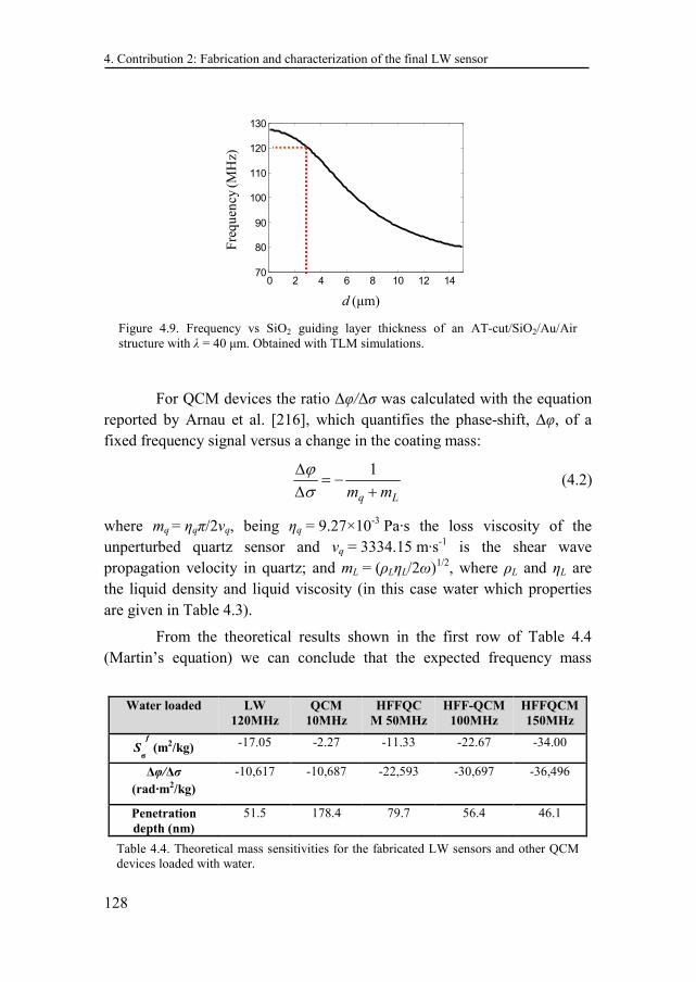
4. Contribution 2: Fabrication and characterization of the final LW sensor
128
For QCM devices the ratio ∆φ/∆σ was calculated with the equation reported by Arnau et al. [216], which quantifies the phase-shift, ∆φ, of a fixed frequency signal versus a change in the coating mass:
1
q Lm m
ϕσ
∆= −
∆ + (4.2)
where mq = ηqπ/2vq, being ηq = 9.27×10⁻³ Pa·s the loss viscosity of the unperturbed quartz sensor and vq = 3334.15 m·s-1 is the shear wave propagation velocity in quartz; and mL = (ρLηL/2ω)1/2, where ρL and ηL are the liquid density and liquid viscosity (in this case water which properties are given in Table 4.3).
From the theoretical results shown in the first row of Table 4.4 (Martin’s equation) we can conclude that the expected frequency mass
Figure 4.9. Frequency vs SiO2 guiding layer thickness of an AT-cut/SiO2/Au/Air structure with λ = 40 µm. Obtained with TLM simulations.
0 2 4 6 8 10 12 1470
80
90
100
110
120
130
d (µm)d (µm)
Fre
quen
cy (M
Hz)
Water loaded LW 120MHz
QCM 10MHz
HFFQCM 50MHz
HFF-QCM 100MHz
HFFQCM 150MHz
Sσ
f
(m2/kg) -17.05 -2.27 -11.33 -22.67 -34.00
∆φ/∆σ
(rad·m2/kg)
-10,617 -10,687 -22,593 -30,697 -36,496
Penetration depth (nm)
51.5 178.4 79.7 56.4 46.1
Table 4.4. Theoretical mass sensitivities for the fabricated LW sensors and other QCM devices loaded with water.
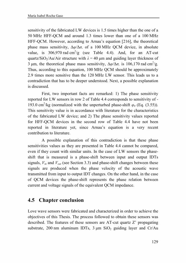
María Isabel Rocha Gaso
129
sensitivity of the fabricated LW devices is 1.5 times higher than the one of a 50 MHz HFF-QCM and around 1.3 times lower than one of a 100 MHz HFF-QCM. However, according to Arnau’s equation [216], the theoretical phase mass sensitivity, ∆φ/∆σ, of a 100 MHz QCM device, in absolute value, is 306,970 rad cm2/g (see Table 4.4). And, for an AT-cut quartz/SiO2/Au/Air structure with λ = 40 µm and guiding layer thickness of 3 µm, the theoretical phase mass sensitivity, ∆φ/∆σ, is 106,170 rad cm2/g. Thus, according to this equation, 100 MHz QCM should be approximately 2.9 times more sensitive than the 120 MHz LW sensor. This leads us to a contradiction that has to be deeper understood. Next, a possible explanation is discussed.
First, two important facts are remarked: 1) The phase sensitivity reported for LW sensors in row 2 of Table 4.4 corresponds to sensitivity of -193.0 cm2/kg (normalized with the unperturbed phase-shift φ0 (Eq. (3.55)). This sensitivity value is in accordance with literature for the characteristics of the fabricated LW device; and 2) The phase sensitivity values reported for HFF-QCM devices in the second row of Table 4.4 have not been reported in literature yet, since Arnau’s equation is a very recent contribution to literature.
A possible explanation of this contradiction is that these phase sensitivities values as they are presented in Table 4.4 cannot be compared, even if they count with similar units. In the case of LW sensors the phase-shift that is measured is a phase-shift between input and output IDTs signals, Vin and Vout (see Section 3.3) and phase-shift changes between these signals are produced when the phase velocity of the acoustic wave transmitted from input to output IDT changes. On the other hand, in the case of QCM devices the phase-shift represents the phase relation between current and voltage signals of the equivalent QCM impedance.
4.5 Chapter conclusion
Love wave sensors were fabricated and characterized in order to achieve the objectives of this Thesis. The process followed to obtain these sensors was described. The features of these sensors are AT-cut quartz Z’ propagating substrate, 200 nm aluminum IDTs, 3 µm SiO2 guiding layer and Cr/Au
4. Contribution 2: Fabrication and characterization of the final LW sensor
130
sensing area. The frequency response of the fabricated device, obtained with a network analyzer, was presented. It is seen that the devices center frequency was of 120.26 ± 0.53 MHz and the insertion loss at this frequency is -21.28 ± 1.07 dB.
María Isabel Rocha Gaso
131
5. Contribution 3: LW microsystem for in liquid
measurements
One of the most common challenges researchers face when dealing with a LW sensor for in liquid applications, as it occurs in biosensors, is the flow cell implementation. The main purpose of a flow cell for LW biosensors is to support and connect the sensor mechanically and electrically to the flow-through and electronic characterization systems, respectively. In addition, the flow cell should allow the flowing liquid to wet the surface of the sensor’s sensing area without leaking into the surrounding area. While these requirements are relatively easy to meet with traditional QCMs, they become considerably more challenging for LW sensors. This is due to the fact that everything in contact with the sensor’s sensing area –like rubber seals– is seen by the propagating acoustic wave as a perturbing obstacle. And the stronger the perturbation is, the more distorted sensor response is produced –this means undesirable higher insertion loss and less linear phase ramp–. Some authors have previously made great efforts regarding this subject [173,217] and there are already some commercially available solutions.
To achieve a user-friendly flow cell, there are even more requirements to be considered. Sagmeister et al. specified some of these requirements for a HFF-QCM flow cell [218]. Among these requirements, the following shall be highlighted, taking into account our system requirements: First, (1) the cell has to allow for fast, easy, and reliable installation and replacement of the sensor. Gluing or pre-wiring of the sensor should be avoided by an effective clamping mechanism. (2) The clamping mechanism has to act on the sensor with a gentle and uniform pressure; a shear-stress across the crystal must not exist. (3) Under no circumstances, liquid must leak through the flow cell/sensor interface. Further, (4) all materials, which get in contact with the liquid, have to be
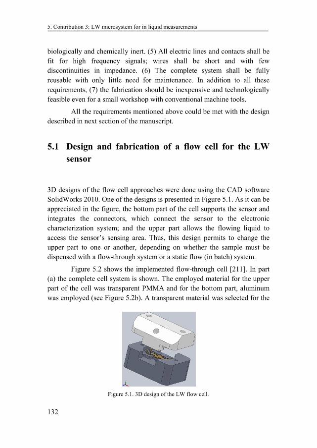
5. Contribution 3: LW microsystem for in liquid measurements
132
biologically and chemically inert. (5) All electric lines and contacts shall be fit for high frequency signals; wires shall be short and with few discontinuities in impedance. (6) The complete system shall be fully reusable with only little need for maintenance. In addition to all these requirements, (7) the fabrication should be inexpensive and technologically feasible even for a small workshop with conventional machine tools.
All the requirements mentioned above could be met with the design described in next section of the manuscript.
5.1 Design and fabrication of a flow cell for the LW
sensor
3D designs of the flow cell approaches were done using the CAD software SolidWorks 2010. One of the designs is presented in Figure 5.1. As it can be appreciated in the figure, the bottom part of the cell supports the sensor and integrates the connectors, which connect the sensor to the electronic characterization system; and the upper part allows the flowing liquid to access the sensor’s sensing area. Thus, this design permits to change the upper part to one or another, depending on whether the sample must be dispensed with a flow-through system or a static flow (in batch) system.
Figure 5.2 shows the implemented flow-through cell [211]. In part (a) the complete cell system is shown. The employed material for the upper part of the cell was transparent PMMA and for the bottom part, aluminum was employed (see Figure 5.2b). A transparent material was selected for the
Figure 5.1. 3D design of the LW flow cell.
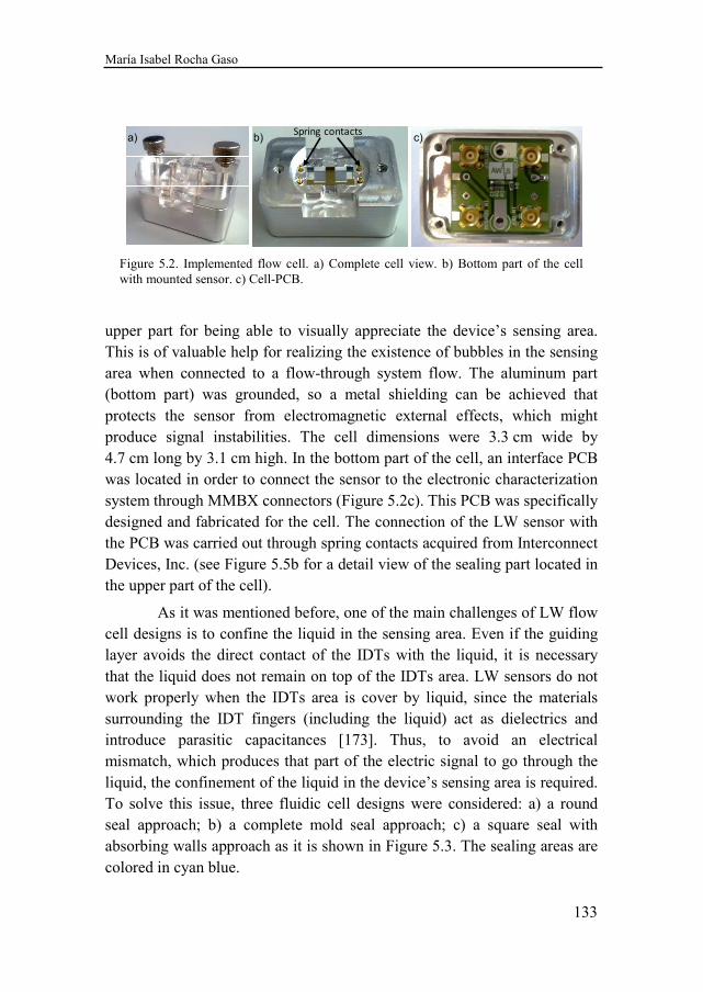
María Isabel Rocha Gaso
133
upper part for being able to visually appreciate the device’s sensing area. This is of valuable help for realizing the existence of bubbles in the sensing area when connected to a flow-through system flow. The aluminum part (bottom part) was grounded, so a metal shielding can be achieved that protects the sensor from electromagnetic external effects, which might produce signal instabilities. The cell dimensions were 3.3 cm wide by 4.7 cm long by 3.1 cm high. In the bottom part of the cell, an interface PCB was located in order to connect the sensor to the electronic characterization system through MMBX connectors (Figure 5.2c). This PCB was specifically designed and fabricated for the cell. The connection of the LW sensor with the PCB was carried out through spring contacts acquired from Interconnect Devices, Inc. (see Figure 5.5b for a detail view of the sealing part located in the upper part of the cell).
As it was mentioned before, one of the main challenges of LW flow cell designs is to confine the liquid in the sensing area. Even if the guiding layer avoids the direct contact of the IDTs with the liquid, it is necessary that the liquid does not remain on top of the IDTs area. LW sensors do not work properly when the IDTs area is cover by liquid, since the materials surrounding the IDT fingers (including the liquid) act as dielectrics and introduce parasitic capacitances [173]. Thus, to avoid an electrical mismatch, which produces that part of the electric signal to go through the liquid, the confinement of the liquid in the device’s sensing area is required. To solve this issue, three fluidic cell designs were considered: a) a round seal approach; b) a complete mold seal approach; c) a square seal with absorbing walls approach as it is shown in Figure 5.3. The sealing areas are colored in cyan blue.
Figure 5.2. Implemented flow cell. a) Complete cell view. b) Bottom part of the cell with mounted sensor. c) Cell-PCB.
a) b) c)Spring contacts
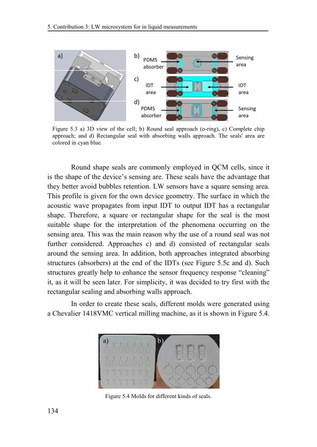
5. Contribution 3: LW microsystem for in liquid measurements
134
Round shape seals are commonly employed in QCM cells, since it is the shape of the device’s sensing are. These seals have the advantage that they better avoid bubbles retention. LW sensors have a square sensing area. This profile is given for the own device geometry. The surface in which the acoustic wave propagates from input IDT to output IDT has a rectangular shape. Therefore, a square or rectangular shape for the seal is the most suitable shape for the interpretation of the phenomena occurring on the sensing area. This was the main reason why the use of a round seal was not further considered. Approaches c) and d) consisted of rectangular seals around the sensing area. In addition, both approaches integrated absorbing structures (absorbers) at the end of the IDTs (see Figure 5.5c and d). Such structures greatly help to enhance the sensor frequency response “cleaning” it, as it will be seen later. For simplicity, it was decided to try first with the rectangular sealing and absorbing walls approach.
In order to create these seals, different molds were generated using a Chevalier 1418VMC vertical milling machine, as it is shown in Figure 5.4.
Figure 5.4 Molds for different kinds of seals.
b)a)
Figure 5.3 a) 3D view of the cell; b) Round seal approach (o-ring), c) Complete chip approach; and d) Rectangular seal with absorbing walls approach. The seals' area are colored in cyan blue.
a) b)
c)
d)PDMS
absorber
IDT
area
IDT
area
Sensing
area
Sensing
areaPDMS
absorber
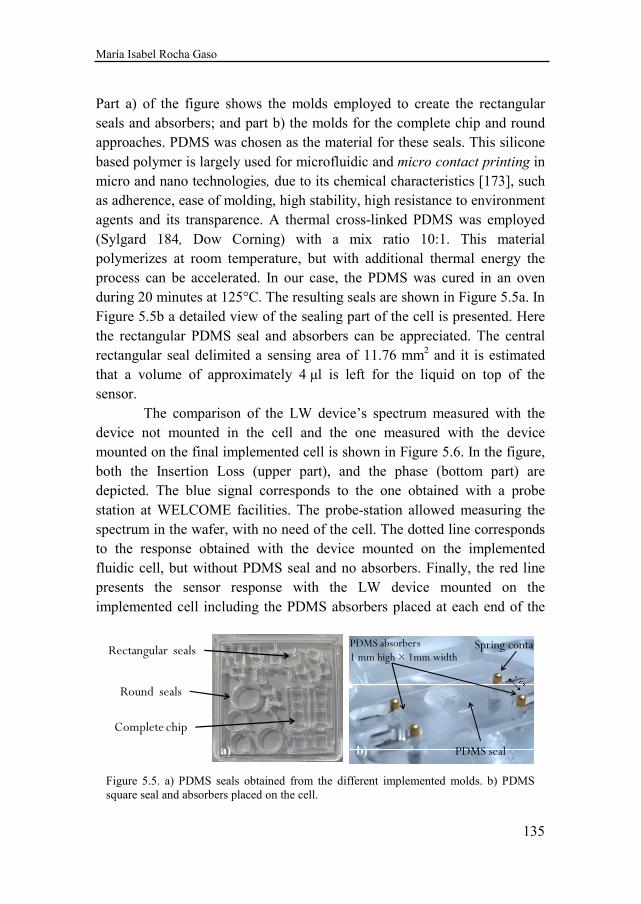
María Isabel Rocha Gaso
135
Part a) of the figure shows the molds employed to create the rectangular seals and absorbers; and part b) the molds for the complete chip and round approaches. PDMS was chosen as the material for these seals. This silicone based polymer is largely used for microfluidic and micro contact printing in micro and nano technologies, due to its chemical characteristics [173], such as adherence, ease of molding, high stability, high resistance to environment agents and its transparence. A thermal cross-linked PDMS was employed (Sylgard 184, Dow Corning) with a mix ratio 10:1. This material polymerizes at room temperature, but with additional thermal energy the process can be accelerated. In our case, the PDMS was cured in an oven during 20 minutes at 125°C. The resulting seals are shown in Figure 5.5a. In Figure 5.5b a detailed view of the sealing part of the cell is presented. Here the rectangular PDMS seal and absorbers can be appreciated. The central rectangular seal delimited a sensing area of 11.76 mm2 and it is estimated that a volume of approximately 4 µl is left for the liquid on top of the sensor. The comparison of the LW device’s spectrum measured with the device not mounted in the cell and the one measured with the device mounted on the final implemented cell is shown in Figure 5.6. In the figure, both the Insertion Loss (upper part), and the phase (bottom part) are depicted. The blue signal corresponds to the one obtained with a probe station at WELCOME facilities. The probe-station allowed measuring the spectrum in the wafer, with no need of the cell. The dotted line corresponds to the response obtained with the device mounted on the implemented fluidic cell, but without PDMS seal and no absorbers. Finally, the red line presents the sensor response with the LW device mounted on the implemented cell including the PDMS absorbers placed at each end of the
Figure 5.5. a) PDMS seals obtained from the different implemented molds. b) PDMS square seal and absorbers placed on the cell.
PDMS absorbers1 mm high × 1mm width
PDMS seal
Spring contacts
a) b)
Round seals
Rectangular seals
Complete chip
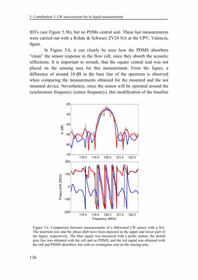
5. Contribution 3: LW microsystem for in liquid measurements
136
IDTs (see Figure 5.5b), but no PDMs central seal. These last measurements were carried out with a Rohde & Schwarz ZV24 NA at the UPV, Valencia, Spain. In Figure 5.6, it can clearly be seen how the PDMS absorbers “clean” the sensor response in the flow cell, since they absorb the acoustic reflections. It is important to remark, that the square central seal was not placed on the sensing area for this measurement. From the figure, a difference of around 10 dB in the base line of the spectrum is observed when comparing the measurements obtained for the mounted and the not mounted device. Nevertheless, since the sensor will be operated around the synchronous frequency (center frequency), this modification of the baseline
Figure 5.6. Comparison between measurements of a fabricated LW sensor with a NA. The insertion loss and the phase-shift have been depicted in the upper and lower part of the figure, respectively. The blue signal was measured with a probe station; the dotted gray line was obtained with the cell and no PDMS; and the red signal was obtained with the cell and PDMS absorbers, but with no rectangular seal on the sensing area.
118.5 119.5 120.5 121.5 122.5-200
-100
0
100
200
Frequency (MHz)
Phase s
hift
(DE
G)
118.5 119.5 120.5 121.5 122.5-70
-60
-50
-40
-30
-20
IL (
dB
)
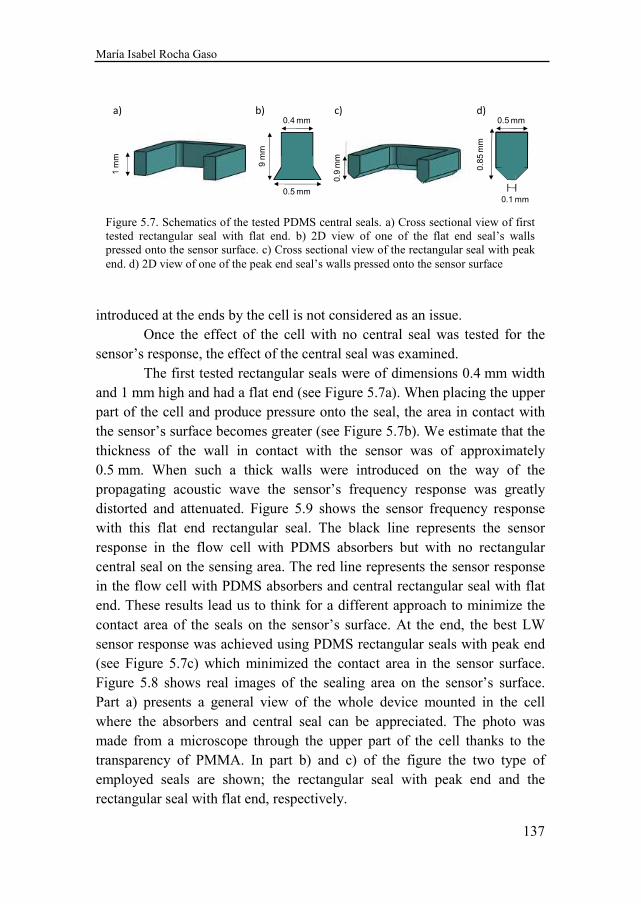
María Isabel Rocha Gaso
137
introduced at the ends by the cell is not considered as an issue. Once the effect of the cell with no central seal was tested for the sensor’s response, the effect of the central seal was examined. The first tested rectangular seals were of dimensions 0.4 mm width and 1 mm high and had a flat end (see Figure 5.7a). When placing the upper part of the cell and produce pressure onto the seal, the area in contact with the sensor’s surface becomes greater (see Figure 5.7b). We estimate that the thickness of the wall in contact with the sensor was of approximately 0.5 mm. When such a thick walls were introduced on the way of the propagating acoustic wave the sensor’s frequency response was greatly distorted and attenuated. Figure 5.9 shows the sensor frequency response with this flat end rectangular seal. The black line represents the sensor response in the flow cell with PDMS absorbers but with no rectangular central seal on the sensing area. The red line represents the sensor response in the flow cell with PDMS absorbers and central rectangular seal with flat end. These results lead us to think for a different approach to minimize the contact area of the seals on the sensor’s surface. At the end, the best LW sensor response was achieved using PDMS rectangular seals with peak end (see Figure 5.7c) which minimized the contact area in the sensor surface. Figure 5.8 shows real images of the sealing area on the sensor’s surface. Part a) presents a general view of the whole device mounted in the cell where the absorbers and central seal can be appreciated. The photo was made from a microscope through the upper part of the cell thanks to the transparency of PMMA. In part b) and c) of the figure the two type of employed seals are shown; the rectangular seal with peak end and the rectangular seal with flat end, respectively.
Figure 5.7. Schematics of the tested PDMS central seals. a) Cross sectional view of first tested rectangular seal with flat end. b) 2D view of one of the flat end seal’s walls pressed onto the sensor surface. c) Cross sectional view of the rectangular seal with peak end. d) 2D view of one of the peak end seal’s walls pressed onto the sensor surface
a) b)0.4 mm
9 m
m
c) d)0.5 mm
0.8
5 m
m
1 m
m
0.1 mm
0.9
mm
0.5 mm
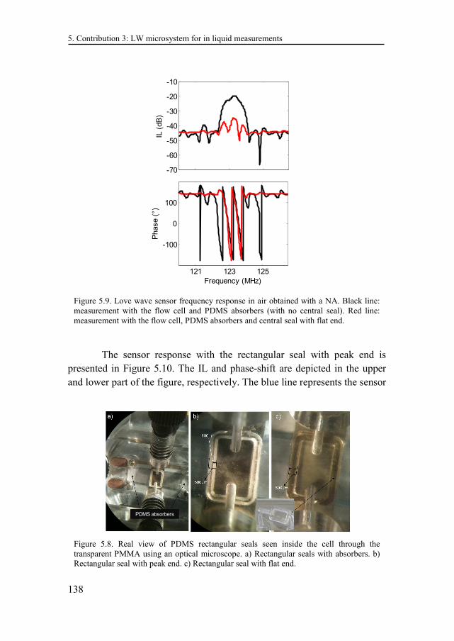
5. Contribution 3: LW microsystem for in liquid measurements
138
The sensor response with the rectangular seal with peak end is presented in Figure 5.10. The IL and phase-shift are depicted in the upper and lower part of the figure, respectively. The blue line represents the sensor
Figure 5.9. Love wave sensor frequency response in air obtained with a NA. Black line: measurement with the flow cell and PDMS absorbers (with no central seal). Red line: measurement with the flow cell, PDMS absorbers and central seal with flat end.
121 123 125-70
-60
-50
-40
-30
-20
-10
IL (
dB
)
121 123 125
-100
0
100
Frequency (MHz)
Phase (
°)
Figure 5.8. Real view of PDMS rectangular seals seen inside the cell through the transparent PMMA using an optical microscope. a) Rectangular seals with absorbers. b) Rectangular seal with peak end. c) Rectangular seal with flat end.
PDMS absorbers
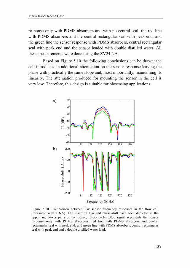
María Isabel Rocha Gaso
139
response only with PDMS absorbers and with no central seal; the red line with PDMS absorbers and the central rectangular seal with peak end; and the green line the sensor response with PDMS absorbers, central rectangular seal with peak end and the sensor loaded with double distilled water. All these measurements were done using the ZV24 NA.
Based on Figure 5.10 the following conclusions can be drawn: the cell introduces an additional attenuation on the sensor response leaving the phase with practically the same slope and, most importantly, maintaining its linearity. The attenuation produced for mounting the sensor in the cell is very low. Therefore, this design is suitable for biosensing applications.
Figure 5.10. Comparison between LW sensor frequency responses in the flow cell (measured with a NA). The insertion loss and phase-shift have been depicted in the upper and lower parts of the figure, respectively. Blue signal represents the sensor response only with PDMS absorbers; red line with PDMS absorbers and central rectangular seal with peak end; and green line with PDMS absorbers, central rectangular seal with peak end and a double distilled water load.
121 122 123 124 125 126-70
-60
-50
-40
-30
-20
-10
121 122 123 124 125 126-200
-100
0
100
200
Frequency (MHz)Frequency (MHz)
Pha
se-s
hift
(D
EG
)IL
(dB
)
a)
b)
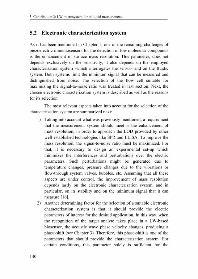
5. Contribution 3: LW microsystem for in liquid measurements
140
5.2 Electronic characterization system
As it has been mentioned in Chapter 1, one of the remaining challenges of piezoelectric immunosensors for the detection of low molecular compounds is the enhancement of surface mass resolution. This parameter, does not depends exclusively on the sensitivity, it also depends on the employed characterization system -which interrogates the sensor- and on the fluidic system. Both systems limit the minimum signal that can be measured and distinguished from noise. The selection of the flow cell suitable for maximizing the signal-to-noise ratio was treated in last section. Next, the chosen electronic characterization system is described as well as the reasons for its selection.
The most relevant aspects taken into account for the selection of the characterization system are summarized next:
1) Taking into account what was previously mentioned, a requirement that the measurement system should meet is the enhancement of mass resolution, in order to approach the LOD provided by other well established technologies like SPR and ELISA. To improve the mass resolution, the signal-to-noise ratio must be maximized. For that, it is necessary to design an experimental set-up which minimizes the interferences and perturbations over the electric parameters. Such perturbations might be generated due to temperature changes, pressure changes due to the vibrations or flow-through system valves, bubbles, etc. Assuming that all these aspects are under control, the improvement of mass resolution depends lastly on the electronic characterization system, and in particular, on its stability and on the minimum signal that it can measure [16].
2) Another determining factor for the selection of a suitable electronic characterization system is that it should provide the electric parameters of interest for the desired application. In this way, when the recognition of the target analyte takes place in a LW-based biosensor, the acoustic wave phase velocity changes, producing a phase-shift (see Chapter 3). Therefore, this phase-shift is one of the parameters that should provide the characterization system. For certain conditions, this parameter solely is sufficient for the
María Isabel Rocha Gaso
141
applications. Such is the case when the recognition of the target analyte only produces mass changes of the coating layer. To assure that only mass changes are taking place (micro gravimetric regime) a second parameter is extremely useful; this is the sensor insertion loss (IL). Some authors have been studying the ratio of IL changes over phase-shift changes (∆IL/∆φ) for biosensing applications [11,159]. They state that such ratio provides valuable information regarding the viscoelastic properties of the coating layer. Hence, taking into account the main objective of this Thesis, which is the development of a biosensor, it was established that the measurement system should provide both signals, the IL and phase-shift. In this way, the additional information regarding viscoelastic effects during the immunoassays can be obtained.
3) One challenge of piezoelectric immunosensors is the multi-analyte detection. Other immunochemical techniques, such as ELISA, allows for this feature. Therefore, this aspect is a weak point about piezoelectric immunosensors and has limited their use as an analytical chemistry technique. Thus, to make a step forward on this issue, the characterization system should be fast enough to allow the characterization of multiple sensors in a reasonable time.
4) It is also of interest that the characterization system be small enough for being portable, of low cost and poses a high integration capability11 for promoting the use of the biosensing system out from laboratories.
Considering the enumerated requirements, Network Analyzers (NA) were dismissed. Even if such instruments provide the sensor IL and phase-shift, they do not fulfill the integration requirement, neither the small size nor the low cost. Moreover, the use of NA can limit the system requirement of ease of extension to array applications.
On the other hand, oscillators meet the requirements of low cost, small size and integration capability. They could be the more suitable for array applications. However, in general, they do not provide direct information of the amplitude of the sensor´s response and their poor stability in high frequency prevents improving the mass resolution (see Section 3.3). 11 The integration capacity consists on the possibility to incorporate the sensor in the same chip than the electronic system's circuitry.
5. Contribution 3: LW microsystem for in liquid measurements
142
Recently, Arnau et al. proposed and validated a new characterization technique which allows improving the mass resolution for QCM and HFF-QCM sensors [187,188,219]. Moreover, such technique fulfills the rest of requirements of the sought characterization system: it provides phase-shift and IL, it is simple, small, fast and it has a high integration capacity. For these reasons, it was chosen as the characterization system of the LW sensors fabricated in this Thesis. The characterization system employed in this thesis is practically the same than the one implemented for QCM and HFF-QCM, but only some slight modifications needed to adapt it to LW sensors. Before actually describing these modifications, next lines provide a brief and general explanation of the operating principle and main blocks of Arnau et al. characterization system. A more detailed explanation can be found in references [187,188,219-221].
5.2.1 Electronic characterization system for QCM resonators
The characterization system proposed by Arnau et al. was conceived as an alternative to the well-known oscillators for HFF-QCM. Oscillators’ theory establishes that the oscillation frequency in an oscillator circuit is the one that satisfies the phase balance equation in the feedback loop. In this equation, the phase of each element of the loop contributes, including the sensor itself. When a biosensor employs an oscillator as the characterization system, it is sought: 1) that the only element of the circuit whose phase changes while the recognition of the target analyte is taking place is the one of the sensor, and 2) that the phase of the rest of elements remain constant. Nonetheless, in practice, the phase of these elements varies, producing noise in the oscillating frequency. This phase noise plays an important role when increasing the operating frequency, limiting the minimum detectable signal and, therefore, the sensitivity [19]. This is the reason why oscillators are not the most suitable characterization technique when working with HFF-QCMs. For these devices, a phase-shift characterization concept, proposed by Arnau et al., was proved as an alternative to increase mass resolution maximizing the signal-to-noise ratio. This characterization technique is based on measuring the sensor’s phase-shifts when it is forced to operate at a fix frequency instead of measuring the sensor’s frequency-shifts due to changes in its phase as oscillators do (this idea is depicted in Figure 5.11).
María Isabel Rocha Gaso
143
In this way, the sensor is interrogated with an appropriate constant frequency signal in a passive way, contrary to what happens in an oscillator, where the sensor plays an active role in the measurement system. This operation mode based on an open loop configuration offers the following advantages: 1) the sensor is a passive element, therefore, the system can be calibrated for setting the characterization system’s operation; 2) the sensor is interrogated with an external source which can be designed to be very stable, and with extremely low phase and frequency noises, even at very high frequencies, which helps minimizing the system noise; 3) the phase-shifts due to the experimental processes that are taking place on the sensor surface can be continuously monitored even for very fast changes in the sensor response while maintaining a fix frequency of the testing signal [188]; and 4) phase-shift measurements can be developed with simple, low cost and electronic subsystems with a high integration capacity.
The general block diagram of the electronic system implemented and tested for QCMs and HFF-QCMs is introduced in Figure 5.12. Two parts can be distinguished in the circuit: the sensor circuit (inside the dashed line) -which includes the sensor- and the control & communication system.
The sensor circuit is formed by two parallel branches, the sensor branch (containing the sensor) and the reference branch, which form a differential circuit. Both branches are exited with the same test signal ut generated by the control & communications system. For more information
Figure 5.11. Description of the phase-shift characterization versus the frequency-shift method (taken from [186]).
∆φ
φ
fft
2
1∆φ
φ
fft
2
1
∆f
Frequency-Shift
Phase-Shift∆φ
φ
fft
2
1∆φ
φ
fft
2
1
∆f
Frequency-Shift
Phase-Shift∆φ
φ
fft
2
1∆φ
φ
fft
2
1
∆f
Frequency-Shift
Phase-Shift
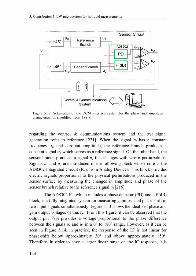
5. Contribution 3: LW microsystem for in liquid measurements
144
regarding the control & communications system and the test signal generation refer to reference [221]. When the signal ut has a constant frequency, ft, and constant amplitude, the reference branch produces a constant signal u1 which serves as a reference signal. On the other hand, the sensor branch produces a signal u2 that changes with sensor perturbations. Signals u1 and u2 are introduced in the following block whose core is the AD8302 Integrated Circuit (IC), from Analog Devices. This block provides electric signals proportional to the physical perturbations produced in the sensor surface by measuring the changes in amplitude and phase of the sensor branch relative to the reference signal u1 [216].
The AD8302 IC, which includes a phase-detector (PD) and a P(dB) block, is a fully integrated system for measuring gain/loss and phase-shift of two input signals simultaneously. Figure 5.13 shows the idealized phase and gain output voltages of this IC. From this figure, it can be observed that the output pin VPHS provides a voltage proportional to the phase difference between the signals u1 and u2 in a 0° to 180° range. However, as it can be seen in Figure 5.14, in practice, the response of the IC is not linear for phase-shift below approximately 30° and above approximately 150°. Therefore, in order to have a larger linear range on the IC response, it is
Figure 5.12. Schematics of the QCM interface system for the phase and amplitude characterization (modified from [188]).
+45°
-45°
ut
u1
u2
PD
AD8302
P(dB)
Control & Communications
System
uφ
uA
Vre
f1
Vre
f2
-
+Adφ
-
+AdA
Vref1
VPHS
VMAG
Vref2
Sensor Circuit
Reference
Branch
Sensor Branch
ui1
ui2
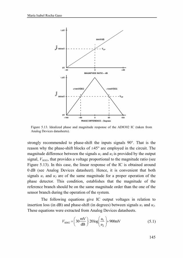
María Isabel Rocha Gaso
145
strongly recommended to phase-shift the inputs signals 90°. That is the reason why the phase-shift blocks of ±45° are employed in the circuit. The magnitude difference between the signals u1 and u2 is provided by the output signal, VMAG, that provides a voltage proportional to the magnitude ratio (see Figure 5.13). In this case, the linear response of the IC is obtained around 0 dB (see Analog Devices datasheet). Hence, it is convenient that both signals u1 and u2 are of the same magnitude for a proper operation of the phase detector. This condition, establishes that the magnitude of the reference branch should be on the same magnitude order than the one of the sensor branch during the operation of the system.
The following equations give IC output voltages in relation to insertion loss (in dB) and phase-shift (in degrees) between signals u1 and u2. These equations were extracted from Analog Devices datasheets.
1
2
mV30 20log 900mV
dBMAG
uV
u
= ⋅ +
(5.1)
Figure 5.13. Idealized phase and magnitude response of the AD8302 IC (taken from Analog Devices datasheets).
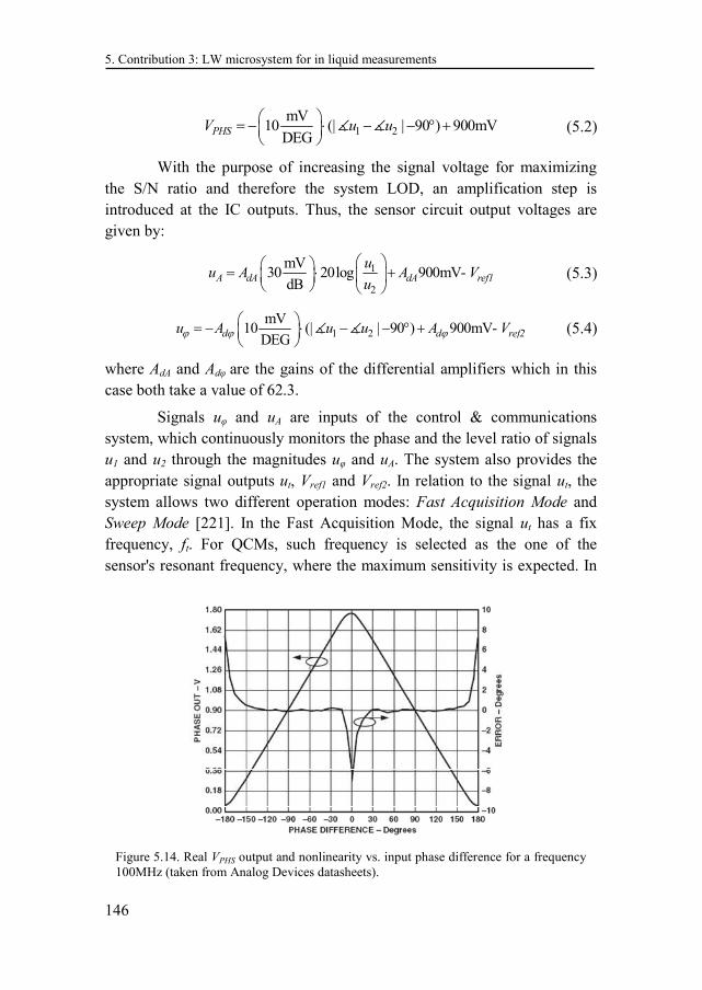
5. Contribution 3: LW microsystem for in liquid measurements
146
1 2mV
10 (| | 90 ) 900mVDEGPHSV u u
= − ⋅ − − ° +
(5.2)
With the purpose of increasing the signal voltage for maximizing the S/N ratio and therefore the system LOD, an amplification step is introduced at the IC outputs. Thus, the sensor circuit output voltages are given by:
1
2
mV30 20log 900mV-
dBA dA dA ref1
uu A A V
u
= ⋅ +
(5.3)
1 2mV
10 (| | 90 ) 900mV- DEGd d ref2u A u u A Vϕ ϕ ϕ
= − ⋅ − − ° +
(5.4)
where AdA and Adφ are the gains of the differential amplifiers which in this case both take a value of 62.3.
Signals uφ and uA are inputs of the control & communications system, which continuously monitors the phase and the level ratio of signals u1 and u2 through the magnitudes uφ and uA. The system also provides the appropriate signal outputs ut, Vref1 and Vref2. In relation to the signal ut, the system allows two different operation modes: Fast Acquisition Mode and Sweep Mode [221]. In the Fast Acquisition Mode, the signal ut has a fix frequency, ft. For QCMs, such frequency is selected as the one of the sensor's resonant frequency, where the maximum sensitivity is expected. In
Figure 5.14. Real VPHS output and nonlinearity vs. input phase difference for a frequency 100MHz (taken from Analog Devices datasheets).
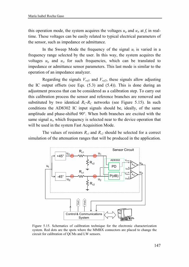
María Isabel Rocha Gaso
147
this operation mode, the system acquires the voltages uφ and uA at ft in real-time. These voltages can be easily related to typical electrical parameters of the sensor, such as impedance or admittance.
In the Sweep Mode the frequency of the signal ut is varied in a frequency range selected by the user. In this way, the system acquires the voltages uφ and uA for such frequencies, which can be translated to impedance or admittance sensor parameters. This last mode is similar to the operation of an impedance analyzer.
Regarding the signals Vref1 and Vref2, these signals allow adjusting the IC output offsets (see Eqs. (5.3) and (5.4)). This is done during an adjustment process that can be considered as a calibration step. To carry out this calibration process the sensor and reference branches are removed and substituted by two identical RC-RC networks (see Figure 5.15). In such conditions the AD8302 IC input signals should be, ideally, of the same amplitude and phase-shifted 90°. When both branches are excited with the same signal ut, which frequency is selected near to the device operation that will be used in the system Fast Acquisition Mode.
The values of resistors Rc1 and Rc2 should be selected for a correct simulation of the attenuation ranges that will be produced in the application.
Figure 5.15. Schematics of calibration technique for the electronic characterization system. Red dots are the spots where the MMBX connectors are placed to change the circuit for calibration of QCMs and LW sensors.
+45°
-45°
ut
u1
u2
PD
AD8302
P(dB)
Control & Communications
System
uφ
uA
Vre
f1
Vre
f2
-
+Adφ
-
+AdA
Vref1
VPHS
VMAG
Vref2
Sensor CircuitRc1
Rc2
Rc1
Rc2
ui1
ui2
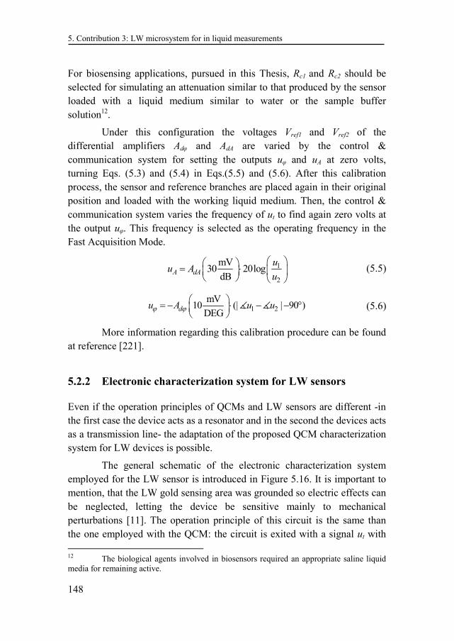
5. Contribution 3: LW microsystem for in liquid measurements
148
For biosensing applications, pursued in this Thesis, Rc1 and Rc2 should be selected for simulating an attenuation similar to that produced by the sensor loaded with a liquid medium similar to water or the sample buffer solution12.
Under this configuration the voltages Vref1 and Vref2 of the differential amplifiers Adφ and AdA are varied by the control & communication system for setting the outputs uφ and uA at zero volts, turning Eqs. (5.3) and (5.4) in Eqs.(5.5) and (5.6). After this calibration process, the sensor and reference branches are placed again in their original position and loaded with the working liquid medium. Then, the control & communication system varies the frequency of ut to find again zero volts at the output uφ. This frequency is selected as the operating frequency in the Fast Acquisition Mode.
1
2
mV30 20log
dBA dA
uu A
u
= ⋅
(5.5)
1 2mV
10 (| | 90 )DEGdu A u uϕ ϕ
= − ⋅ − − °
(5.6)
More information regarding this calibration procedure can be found at reference [221].
5.2.2 Electronic characterization system for LW sensors
Even if the operation principles of QCMs and LW sensors are different -in the first case the device acts as a resonator and in the second the devices acts as a transmission line- the adaptation of the proposed QCM characterization system for LW devices is possible.
The general schematic of the electronic characterization system employed for the LW sensor is introduced in Figure 5.16. It is important to mention, that the LW gold sensing area was grounded so electric effects can be neglected, letting the device be sensitive mainly to mechanical perturbations [11]. The operation principle of this circuit is the same than the one employed with the QCM: the circuit is exited with a signal ut with 12 The biological agents involved in biosensors required an appropriate saline liquid media for remaining active.
María Isabel Rocha Gaso
149
fix frequency ft and the difference in phase-shift and amplitude between signals u1 and u2 are measured. When a perturbation takes place on the surface of the device a change in the phase velocity and energy of the acoustic wave is produced, generating a change in the phase-shift and insertion loss (see Chapter 3). Assuming that the elements of the reference branch remain invariable, the signals uφ and uA can be directly related to the phase-shift and IL produced by the perturbation. A description and analysis of the different blocks required for adapting the HFF-QCM original schematic to LW sensors is given in next lines.
The phase-shifting networks formed by Ri and Ci were designed coherently for a cut-off frequency (−3dB) of 120 MHz (ω = 1 / RiCi) in order to obtain two signals 90º phase-shifted of similar amplitudes to guarantee the optimal operation of the AD8302 IC. Hence, the employed values for this circuit were, 49.9 Ω (1%) and high-Q 25 pF, for Ri and Ci, respectively.
In relation to the sensor branch, a resistor RL is required in order to polarize the amplifier OPA4. To know the convenient value for this resistor the following criteria was used: when RL is introduced in the network, it
Figure 5.16. Schematics of the phase and amplitude interface system for the characterization of the LW sensor. The elements inside the red dotted line were placed in the cell-PCB.
uφ
ut
Ci
Ci
Ri
Ri
R1
RL
R2
LW Sensor
u1
u2
PD
OPA1
OPA2
OPA3
OPA4
AD8302
ft
P(dB) uA
-
+Adφ
-
+AdA
Vref1
VPHS
VMAG
Vref2
cell-PCB
Control & Communications
System
Vre
f1
Vre
f2
ui1
ui2
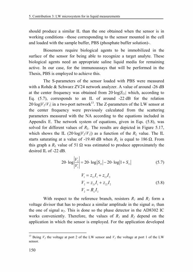
5. Contribution 3: LW microsystem for in liquid measurements
150
should produce a similar IL than the one obtained when the sensor is in working conditions –those corresponding to the sensor mounted in the cell and loaded with the sample buffer, PBS (phosphate buffer solution)-.
Biosensors require biological agents to be immobilized in the surface of the sensor for being able to recognize a target analyte. These biological agents need an appropriate saline liquid media for remaining active. In our case, for the immunoassays that will be performed in the Thesis, PBS is employed to achieve this.
The S-parameters of the sensor loaded with PBS were measured with a Rohde & Schwarz ZV24 network analyzer. A value of around -26 dB at the center frequency was obtained from 20·log|S21| which, according to Eq. (5.7), corresponds to an IL of around -22 dB for the relation 20·log|V2/V1| in a two-port network13. The Z-parameters of the LW sensor at the center frequency were previously calculated from the scattering parameters measured with the NA according to the equations included in Appendix E. The network system of equations, given in Eqs. (5.8), was solved for different values of RL. The results are depicted in Figure 5.17, which shows the IL (20·log|V2/V1|) as a function of the RL value. The IL starts saturating at a value of -19.40 dB when RL is equal to 186 Ω. From this graph a RL value of 51 Ω was estimated to produce approximately the desired IL of -22 dB.
221 11
1
20 log 20 log 20 log 1V
S SV
⋅ = ⋅ − ⋅ + (5.7)
1 11 1 12 2
2 21 1 22 2
2 2L
V z I z I
V z I z I
V R I
= +
= +
=
(5.8)
With respect to the reference branch, resistors R1 and R2 form a voltage divisor that has to produce a similar amplitude in the signal u1 than the one of signal u2. This is done so the phase detector in the AD8302 IC works conveniently. Therefore, the values of R1 and R2 depend on the application in which the sensor is employed. For the application developed
13 Being V2 the voltage at port 2 of the LW sensor and V1 the voltage at port 1 of the LW sensor.
María Isabel Rocha Gaso
151
in this Thesis, the amplitude of u2 will be mainly given by the sensor response in contact with PBS. The immobilization of the required biomolecules over the sensor surface and the adhesion of the antibodies during the detection of the target analyte do not substantially modify the amplitude of the signal u2. Under these conditions, the sensor will produce an attenuation of around -22 dB at the center frequency, choosing values of resistors R1 and R2 of 560 and 49.9 Ω, respectively, the IL introduced by the reference branch is of the same order of magnitude than the one introduced by the sensor. The values of these resistances should be low so at high operating frequencies the resistances behave as ideal as possible.
Once the criteria followed for adapting the different blocks of the electronic characterization system to LW sensors was explained, the equations that relate the phase-shift and insertion loss between the input and output IDT signals from the acquired signals uA and uφ are presented.
In the LW sensor circuit of Figure 5.16 the signal ui1 and u1 in the reference branch are given by the following expressions:
1 1i i
i ti i
j R Cu u
j R C
ωω
=+
(5.9)
21
1 2 1i i
ti i
j R CRu u
R R j R C
ωω
=+ +
(5.10)
Figure 5.17. Insertion loss (IL) versus resistor RL of the LW sensor seen as a two-port network device (X-axis in logarithmic scale).
50 500-50
-40
-30
-20
-10
RL (Ω)
20 lo
g|V
2/V
1| (d
B)
-22
5. Contribution 3: LW microsystem for in liquid measurements
152
While in the sensor branch the signal ui2 is given by:
21
1i ti i
u uj R Cω
=+
(5.11)
After some simple algebra manipulation of Eqs. (5.9) and (5.11), it is possible to arrive to the following equation:
22 2
2 1 1 2
i i
i
j R C Ru u
u u R R
ω=
+ (5.12)
Taking into account that the signals ui2 and u2 represents the signals at the LW sensor input and output ports, respectively, the device IL can be obtained through the following expressions:
22 2
2 1 1 2(dB) 20log 20log 20log i i
i
j R C Ru uIL
u u R R
ω= = +
+ (5.13)
On the other hand, Eq. (5.5), obtained in last section, provides the relation between the IC inputs and it output signal uA as follows:
2
120log
30 mV/dBA
dA
u u
u A= − (5.14)
Using Eqs. (5.11) and (5.12) the IL of the LW sensor can be related with the uA voltage acquired by the control & communication system in the following way:
2 2
2 1 2
20log 20log 30 mV/dB
i i A
i dA
u R C R u
u R R A
ω = − +
(5.15)
In relation to the phase-shift between the voltage signals at the input and output of the LW sensor, Eq. (5.6) provides the phase-shift between the IC input signals in function of the signal uφ acquired by the control & communications system:
2 1 90mV
10DEGd
uu u
A
ϕ
ϕ
− = − − °
(5.16)
Thus, from Eqs. (5.12) and (5.16) the phase-shift of interest is obtained:
María Isabel Rocha Gaso
153
2 2 2 1 90º10
i
d
uu u u u
mVA
DEG
ϕ
ϕ
− = − + =
(5.17)
Regarding the calibration of the LW sensor, it is done in the same way than for the QCM sensor as described in Section 5.2.1.
5.3 Proposed characterization system vs. a reference
instrument
With the purpose of comparing the frequency responses measured with a Network Analyzer (NA) and the ones obtained with the adapted electronic characterization system (ES) for LW sensors presented in last section, next lines presents, the frequency responses obtained for the LW sensor mounted in the fabricated cell with the central rectangular PDMS seal, PDMS absorbers and with two different loading media: 1) air and 2) double distilled water.
Figure 5.18 presents the comparison between the frequency response of the sensor in air obtained with a NA and the one obtained with the proposed ES, applying Eqs. (5.15) and (5.17). To obtain the frequency response with the adapted ES, the sweep operation mode of the system, described in Section 5.2.1, was employed. A frequency range from 119 to 121.5 MHz was selected for the sweep. From this response the ES optimal operating frequency, fop, for starting the Fast Acquisition Mode can be chosen. In the case of LW sensors devices the selected operating frequency is the one at which the IL is minimum and at which the phase-shift is 0° (see Figure 5.18). It can be appreciated how the IL responses have similar shapes and values in the central part of the response (around the center frequency), but not at the ends. This is due to the fact that the AD8302 IC is able to measure correctly the IL between the signals u1 and u2 up to a limited attenuation. When this threshold is exceeded, the IC does not operate accurately. In addition, the reference branch (Figure 5.16) was designed for the device minimum insertion loss, which occurs at the device center frequency, and the calibration procedure is carried out around this frequency. Thus, getting too far from the device center frequency introduces inaccurate results.
5. Contribution 3: LW microsystem for in liquid measurements
154
On the other hand, in Figure 5.18 the profile of the phase-shift given by the ES has a different shape due to the real output response VPHS of the AD8302 IC (see Figure 5.14). Nevertheless, it can clearly been appreciated in the figure that the ES response peak-to-peak corresponds to 360° of the peak-to-peak NA response, what it is expected from the IC response.
Figure 5.19 and Figure 5.20 show the frequency responses of the water loaded LW sensor mounted in the flow cell. Such measurements were performed with the NA14 and adapted ES, respectively. In both figures, the solid line represents the IL and the dotted line represents the phase-shift. A minimum IL of approximately -28 dB was observed in the response obtained with the NA (Figure 5.19). Figure 5.20 shows the frequency response obtained with the ES (relation between u2 and ui2) after applying
14 SMA connectors were used for this measurement.
Figure 5.18 LW sensor frequency response mounted in the cell and sensor in contact with air. The solid line represents the measurements obtained with a Network Analyzer (NA) and the dotted line the measurements obtained with the implemented electronic characterization system (ES).
119.5 120 120.5 121-70
-60
-50
-40
-30
-20
IL (
dB
)
5
20 log |S21
| NA
20 log |u2/u
i2| ES
119.5 120 120.5 121-200
-100
0
100
200
Frequency (MHz)
Phase (
DE
G)
phase of S21
NA
phase of u2/u
i2 ES
Working point
María Isabel Rocha Gaso
155
Eqs.(5.15) and (5.17). A minimum IL around -32 dB was measured in this response at the device center frequency.
A study of reproducibility of the measurements performed with the developments of this Thesis was carried out. The frequency response of one sensor, mounted in the fabricated flow-through cell, was obtained with the ES. The optimal operation frequency was determined and the slope of the curve phase-shift voltage versus frequency around this frequency was measured. The flow-through cell was disconnected from the ES and the sensor was removed and mounted again in the cell for performing the same measurement. This procedure was repeated for 11 times (n = 11) obtaining a slope of -453.93 ± 1.52 µV/Hz. Therefore, a good reproducibility was observed.
5.4 Chapter conclusion
Along this chapter the design and fabrication of a flow cell for the LW sensor was described. The adapted electronic characterization system for the LW sensors was also presented as well as some measurements carried out with the flow cell and electronic characterization system. These results were satisfactory for carrying out in liquid measurements with the LW sensors.
Figure 5.19. LW sensor frequency response with the cell and in contact with double distilled water. The measurement of this frequency response was obtained with a NA. The solid line represents the IL loss and the dotted line represents the phase-shift.
119.5 120 120.5 121-60
-50
-40
-30
-20
IL (
dB
)
119.5 120 120.5 121-200
-100
0
100
200
Frequency (MHz)
Phase s
hift
(DE
G)
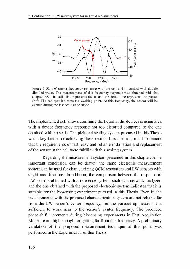
5. Contribution 3: LW microsystem for in liquid measurements
156
The implemented cell allows confining the liquid in the devices sensing area with a device frequency response not too distorted compared to the one obtained with no seals. The pick-end sealing system proposed in this Thesis was a key factor for achieving these results. It is also important to remark that the requirements of fast, easy and reliable installation and replacement of the sensor in the cell were fulfill with this sealing system.
Regarding the measurement system presented in this chapter, some important conclusion can be drawn: the same electronic measurement system can be used for characterizing QCM resonators and LW sensors with slight modifications. In addition, the comparison between the response of LW sensors obtained with a reference system, such as a network analyzer, and the one obtained with the proposed electronic system indicates that it is suitable for the biosensing experiment pursued in this Thesis. Even if, the measurements with the proposed characterization system are not reliable far from the LW sensor’s center frequency, for the pursued application it is sufficient to work near to the sensor’s center frequency. The produced phase-shift increments during biosensing experiments in Fast Acquisition Mode are not high enough for getting far from this frequency. A preliminary validation of the proposed measurement technique at this point was performed in the Experiment 1 of this Thesis.
Figure 5.20. LW sensor frequency response with the cell and in contact with double distilled water. The measurement of this frequency response was obtained with the adapted ES. The solid line represents the IL and the dotted line represents the phase-shift. The red spot indicates the working point. At this frequency, the sensor will be excited during the fast acquisition mode.
119.5 120 120.5 121
-40
-38
-36
-34
-32
IL (
dB
)
-80
-40
0
40
80
Frequency (MHz)
Phase-s
hift
(DE
G)
Working point
María Isabel Rocha Gaso
157
6. Experimental section
6.1 Introduction
Two main experimental contributions were carried out in the frame of this Thesis. The purpose of the first one was to validate the implemented characterization technique, adapted for LW sensors (described in Section 5.2.3) using a reference instrument and comparing with theoretical values. The second one was thought to validate the developments implemented in this Thesis for LW technology in biosensing application and compare it performance with other sensing technologies, including the traditional QCM and HFF-QCM technologies.
Experiment 1: “Measurements of glycerol-water solutions”. Measurements of phase-shift and amplitude for different concentrations of glycerol-water solutions were performed with the electronic characterization system adapted for LW sensors and with a network analyzer for determining the reliability and accurateness of the implemented characterization system.
Experiment 2: “Carbaryl immunosensor”. A LW based immunosensor for detection of carbaryl insecticide was developed. The results of this application will allow us to compare the obtained experimental values with the ones previously obtained for carbaryl immunosensors developed based on other detection technologies.
Next, the materials and methods as well as the results and discussion of both experiments are described.
6. Experimental section
158
6.2 Experiment 1: Measurements of glycerol-water
solutions
The purpose of this experiment was to determine whether the adapted electronic characterization (ES) system for LW sensors was reliable and provided the same phase-shift and amplitude-shift than the theoretical models and the ones obtained with a network analyzer (NA). To accomplish this purpose, the response of the LW sensor was investigated measuring phase-shift and amplitude for different concentrations of glycerol-water solutions with the ES and a NA, this last considered as the reference. Furthermore, the results were compared with the ones obtained with transmission line model (TLM) simulations of the fabricated LW sensor structure. Next, the materials and methods employed for this experiment are mentioned.
6.2.1 Materials and Methods
6.2.1.1 Electronic characterization system
The employed electronic characterization system (ES) was the one described in Section 5.2.2. The ES is based on phase-shift and amplitude measurements at constant frequency. Figure 6.1 presents the picture of the employed test platform that integrates such characterization system with the fabricated LW flow cell; a flow circuit with automated syringe pumps, distribution and injection valves; and a thermal control unit. However, for this experiment the platform fluidic module was not employed. The A10 test platform can be connected through Ethernet to an external computer were the acquisition software is run. Such platform was developed during the Thesis of García-Narbón on HFF-QCM resonators [221] and it is currently commercialized by the company AWSensors, Valencia, Spain.
6.2.1.2 Network Analyzer
The NA measurements were carried out using a two-port Rohde & Schwarz ZV24 network analyzer (Figure 6.2). This NA works in a frequency range
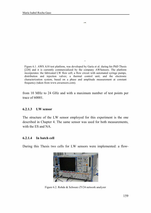
María Isabel Rocha Gaso
from 10 MHz to 24 GHz and with a maximumtrace of 60001.
6.2.1.3 LW sensor
The structure of the LW sensor employed described in Chapter 4. The same sensor was used for both mwith the ES and NA.
6.2.1.4 In batch cell
During this Thesis two cells for LW sensors were implemented: a flow
Figure 6.2. Rohde & Schwarz ZV24 network analyzer
Figure 6.1. AWS A10 test platform, was developed by Gar[220] and it is currently commercialized by the company AWSensors. The platformincorporates: the fabricated LW flow cell; a flow circuit with automated syringe pumps, distribution and injection valves; a thermal control unit; characterization system, based on a phase and amplitude frequency (taken from www.awsensors.com).
159
maximum number of test points per
employed for this experiment is the one sensor was used for both measurements,
During this Thesis two cells for LW sensors were implemented: a flow-
Rohde & Schwarz ZV24 network analyzer
. AWS A10 test platform, was developed by Garía et al. during his PhD Thesis
currently commercialized by the company AWSensors. The platform flow cell; a flow circuit with automated syringe pumps,
distribution and injection valves; a thermal control unit; and the electronic and amplitude measurement at constant
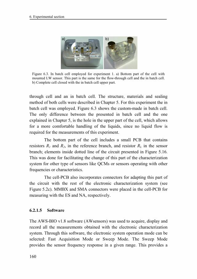
6. Experimental section
160
through cell and an in batch cell. The structure, materials and sealing method of both cells were described in Chapter 5. For this experiment the in batch cell was employed. Figure 6.3 shows the custom-made in batch cell. The only difference between the presented in batch cell and the one explained in Chapter 5, is the hole in the upper part of the cell, which allows for a more comfortable handling of the liquids, since no liquid flow is required for the measurements of this experiment.
The bottom part of the cell includes a small PCB that contains resistors R1 and R2, in the reference branch, and resistor RL in the sensor branch; elements inside dotted line of the circuit presented in Figure 5.16. This was done for facilitating the change of this part of the characterization system for other type of sensors like QCMs or sensors operating with other frequencies or characteristics.
The cell-PCB also incorporates connectors for adapting this part of the circuit with the rest of the electronic characterization system (see Figure 5.2c). MMBX and SMA connectors were placed in the cell-PCB for measuring with the ES and NA, respectively.
6.2.1.5 Software
The AWS-BIO v1.8 software (AWsensors) was used to acquire, display and record all the measurements obtained with the electronic characterization system. Through this software, the electronic system operation mode can be selected: Fast Acquisition Mode or Sweep Mode. The Sweep Mode provides the sensor frequency response in a given range. This provides a
Figure 6.3. In batch cell employed for experiment 1. a) Bottom part of the cell with mounted LW sensor. This part is the same for the flow-through cell and the in batch cell. b) Complete cell closed with the in batch cell upper part.
a) b)
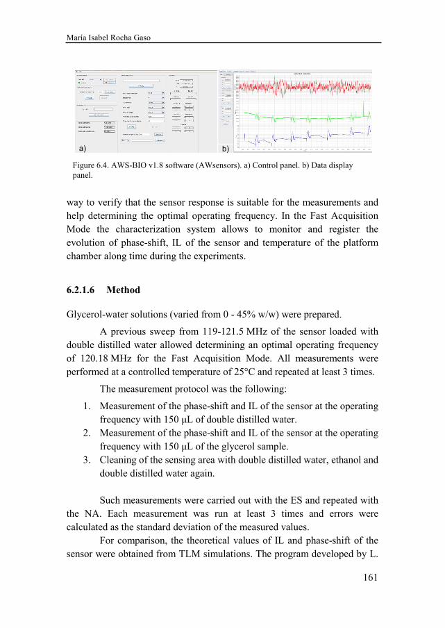
María Isabel Rocha Gaso
161
way to verify that the sensor response is suitable for the measurements and help determining the optimal operating frequency. In the Fast Acquisition Mode the characterization system allows to monitor and register the evolution of phase-shift, IL of the sensor and temperature of the platform chamber along time during the experiments.
6.2.1.6 Method
Glycerol-water solutions (varied from 0 - 45% w/w) were prepared.
A previous sweep from 119-121.5 MHz of the sensor loaded with double distilled water allowed determining an optimal operating frequency of 120.18 MHz for the Fast Acquisition Mode. All measurements were performed at a controlled temperature of 25°C and repeated at least 3 times.
The measurement protocol was the following:
1. Measurement of the phase-shift and IL of the sensor at the operating frequency with 150 µL of double distilled water.
2. Measurement of the phase-shift and IL of the sensor at the operating frequency with 150 µL of the glycerol sample.
3. Cleaning of the sensing area with double distilled water, ethanol and double distilled water again.
Such measurements were carried out with the ES and repeated with the NA. Each measurement was run at least 3 times and errors were calculated as the standard deviation of the measured values. For comparison, the theoretical values of IL and phase-shift of the sensor were obtained from TLM simulations. The program developed by L.
Figure 6.4. AWS-BIO v1.8 software (AWsensors). a) Control panel. b) Data display panel.
a) b)
6. Experimental section
162
Francis [11] was used. The considered four-layer model (see Figure 3.1) was formed by: 1) the piezoelectric substrate; 2) the guiding layer; 3) the sensing area; and 4) the semi-infinite fluid medium (in this case glycerol). The material properties used for the simulations were the same presented in Table 4.3. Density and viscosity properties of the different glycerol-water solutions were extracted from [222]. In order to choose the optimal operating frequency of the sensor measured with the electronic characterization system (ES) and a network analyzer (NA), sweeps were carried out with the same sensor in contact with 0% glycerol-water solution (double distilled water) with both equipments. Figure 5.19 and Figure 5.20 show the sensor’s frequency response obtained with the NA and ES, respectively. The sensor’s operating frequency, for each instrument, was chosen in such way that the conditions of 0 DEG of phase-shift and minimum IL were met. Next, the results obtained in this experiment are presented and discussed.
6.2.2 Results and discussion
The selected operation frequencies were of 120.31 and 120.18 MHz for the NA and ES, respectively. The difference in such frequency might be due to the use of different cell connectors (SMA and MMBX connectors, for measuring with the NA and ES, respectively) and the difference in pressure of the seal in contact with the sensor, due to a lack of cell optimization. However, it is considered that such difference in the operating frequency will not affect the results of this experiment. Phase-shift φ and IL changes at such operation frequencies measured for different concentrations of glycerol-water solutions are presented in Table 6.1. The φ and IL of 0% glycerol solution (water) were considered as zero and were set as the reference measurements. The minus sign in the phase indicates that the phase velocity of the sensing event is lower with respect to the unperturbed event15 phase velocity (0% glycerol solution). Figure 6.5 shows the complete LW sensor’s frequency responses for the different glycerol
15 Remember ∆vφ = vφ- vφ0,where vφ0 is the unperturbed phase velocity and vφ is the perturbed phase velocity.
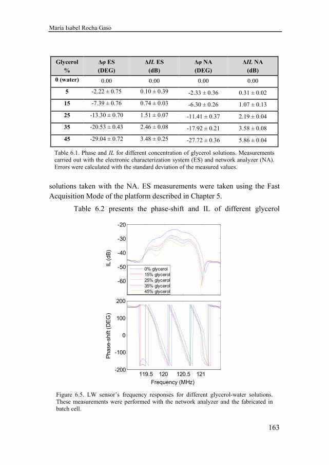
María Isabel Rocha Gaso
163
solutions taken with the NA. ES measurements were taken using the Fast Acquisition Mode of the platform described in Chapter 5.
Table 6.2 presents the phase-shift and IL of different glycerol
Glycerol
%
∆φ ES
(DEG)
∆IL ES
(dB)
∆φ NA
(DEG)
∆IL NA
(dB)
0 (water) 0.00 0.00 0.00 0.00
5 -2.22 ± 0.75 0.10 ± 0.39 -2.33 ± 0.36 0.31 ± 0.02
15 -7.39 ± 0.76 0.74 ± 0.03 -6.30 ± 0.26 1.07 ± 0.13
25 -13.30 ± 0.70 1.51 ± 0.07 -11.41 ± 0.37 2.19 ± 0.04
35 -20.53 ± 0.43 2.46 ± 0.08 -17.92 ± 0.21 3.58 ± 0.08
45 -29.04 ± 0.72 3.48 ± 0.25 -27.72 ± 0.36 5.86 ± 0.04
Table 6.1. Phase and IL for different concentration of glycerol solutions. Measurements carried out with the electronic characterization system (ES) and network analyzer (NA). Errors were calculated with the standard deviation of the measured values.
Figure 6.5. LW sensor’s frequency responses for different glycerol-water solutions. These measurements were performed with the network analyzer and the fabricated in batch cell.
119.5 120 120.5 121 -70
-60
-50
-40
-30
-20
Frequency (MHz)
IL (
dB
)
119.5 120 120.5 121 -200
-100
0
100
200
Phase-s
hift (D
EG
)IL
(dB
)
0% glycerol
15% glycerol
25% glycerol
35% glycerol
45% glycerol
Frequency (MHz)
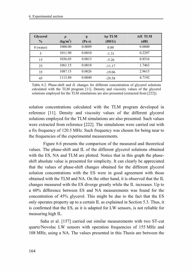
6. Experimental section
164
solution concentrations calculated with the TLM program developed in reference [11]. Density and viscosity values of the different glycerol solutions employed for the TLM simulations are also presented. Such values were extracted from reference [222]. The simulations were carried out with a fix frequency of 120.5 MHz. Such frequency was chosen for being near to the frequencies of the experimental measurements.
Figure 6.6 presents the comparison of the measured and theoretical values. The phase-shift and IL of the different glycerol solutions obtained with the ES, NA and TLM are plotted. Notice that in this graph the phase-shift absolute value is presented for simplicity. It can clearly be appreciated that the values of phase-shift changes obtained for the different glycerol solution concentrations with the ES were in good agreement with those obtained with the TLM and NA. On the other hand, it is observed that the IL changes measured with the ES diverge greatly while the IL increases. Up to a 60% difference between ES and NA measurements was found for the concentration of 45% glycerol. This might be due to the fact that the ES only operates property up to a certain IL as explained in Section 5.3. Thus, it is confirmed that the ES, as it is adapted for LW sensors, is not reliable for measuring high IL.
Saha et al. [157] carried out similar measurements with two ST-cut quartz/Novolac LW sensors with operation frequencies of 155 MHz and 108 MHz, using a NA. The values presented in this Thesis are between the
Glycerol
%
ρ
(kg/m3)
η
(Pa s)
∆φ TLM
(DEG)
∆IL TLM
(dB)
0 (water) 1000.00 0.0009 0.00 0.0000
5 1011.90 0.0010 -1.31 0.2297
15 1036.05 0.0013 -5.26 0.8516
25 1061.15 0.0018 -11.17 1.7463
35 1087.15 0.0026 -19.06 2.9615
45 1113.80 0.0040 -29.58 4.7192
Table 6.2. Phase-shift and IL changes for different concentration of glycerol solutions calculated with the TLM program [11]. Density and viscosity values of the glycerol solutions employed for the TLM simulations are also presented (extracted from [222]).
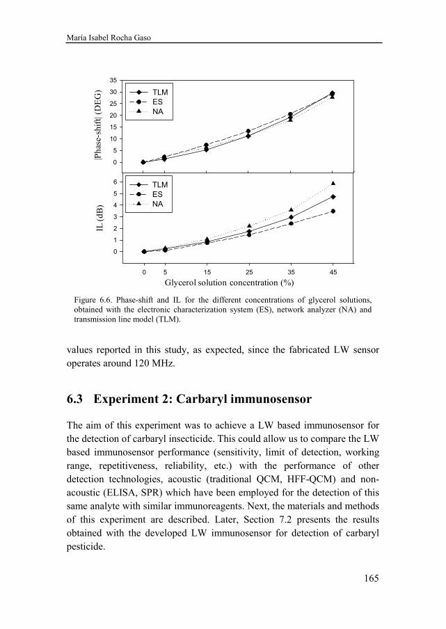
María Isabel Rocha Gaso
165
values reported in this study, as expected, since the fabricated LW sensor operates around 120 MHz.
6.3 Experiment 2: Carbaryl immunosensor
The aim of this experiment was to achieve a LW based immunosensor for the detection of carbaryl insecticide. This could allow us to compare the LW based immunosensor performance (sensitivity, limit of detection, working range, repetitiveness, reliability, etc.) with the performance of other detection technologies, acoustic (traditional QCM, HFF-QCM) and non-acoustic (ELISA, SPR) which have been employed for the detection of this same analyte with similar immunoreagents. Next, the materials and methods of this experiment are described. Later, Section 7.2 presents the results obtained with the developed LW immunosensor for detection of carbaryl pesticide.
Figure 6.6. Phase-shift and IL for the different concentrations of glycerol solutions, obtained with the electronic characterization system (ES), network analyzer (NA) and transmission line model (TLM).
0 5 15 25 35 45
0
1
2
3
4
5
6 TLM
ES
NA
0
5
10
15
20
25
30
35
TLM
ES
NA
|Pha
se-s
hift
| (D
EG
)IL
(dB
)
Glycerol solution concentration (%)
6. Experimental section
166
6.3.1 Materials and methods
6.3.1.1 Chemicals and immunoreagents
Bovine Serum Albumin (BSA) fraction V protein was purchased from Roche Diagnostics (Mannheim, Germany). Tween 20 was supplied by Sigma-Aldrich Chemie (Madrid, Spain). All other chemicals were of analytical grade.
1-Ethyl-3(-3 dimethyl-amino-propyl) carbodiimide hydrochloride (EDC) and N-hydroxysuccinimide (NHS) were purchased from Pierce (Rockford, IL); mercaptohexadecanoic acid (MHDA) was supplied by Sigma–Aldrich Chemie (Madrid, Spain); and ethanolamine blocking agent was obtained from Sigma (St. Louis, MO).
Carbaryl insecticide was purchased from Dr. Ehrenstorfer (Augsburg, Germany). A 1 mM stock dissolution of dimethylformamide (DMF) was prepared and stored at -20°C protected from light in dark vials.
All the immunoreagents were produced by the Immunotechnology Group of I3BH, UPV, Spain. The carbaryl hapten (CNH) the carbaryl hapten conjugate (BSA-CNH) and the carbaryl monoclonal antibody (LIB-CNH45 MAb) were described in previous works [13,31].
6.3.1.1.1 Buffers
• PBS: 10 mM phosphate buffer, pH 7.45.
• PBST: PBS containing 0.005% Tween 20 (working buffer).
• 0.1 M sodium phosphate buffer, pH 7.5.
• 0.1 M sodium borate buffer, pH 8.75.
6.3.1.2 Covalent immobilization
6.3.1.2.1 LW devices clean up
LW devices were first cleaned by immersion into acetone and ethanol, followed by subsequent rinses with double distilled water. Afterwards, the devices were blown dry with a stream of nitrogen gas. Once dried, the
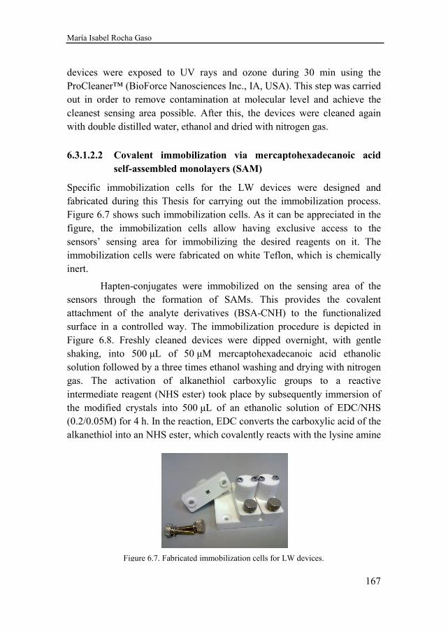
María Isabel Rocha Gaso
167
devices were exposed to UV rays and ozone during 30 min using the ProCleaner™ (BioForce Nanosciences Inc., IA, USA). This step was carried out in order to remove contamination at molecular level and achieve the cleanest sensing area possible. After this, the devices were cleaned again with double distilled water, ethanol and dried with nitrogen gas.
6.3.1.2.2 Covalent immobilization via mercaptohexadecanoic acid
self-assembled monolayers (SAM)
Specific immobilization cells for the LW devices were designed and fabricated during this Thesis for carrying out the immobilization process. Figure 6.7 shows such immobilization cells. As it can be appreciated in the figure, the immobilization cells allow having exclusive access to the sensors’ sensing area for immobilizing the desired reagents on it. The immobilization cells were fabricated on white Teflon, which is chemically inert.
Hapten-conjugates were immobilized on the sensing area of the sensors through the formation of SAMs. This provides the covalent attachment of the analyte derivatives (BSA-CNH) to the functionalized surface in a controlled way. The immobilization procedure is depicted in Figure 6.8. Freshly cleaned devices were dipped overnight, with gentle shaking, into 500 µL of 50 µM mercaptohexadecanoic acid ethanolic solution followed by a three times ethanol washing and drying with nitrogen gas. The activation of alkanethiol carboxylic groups to a reactive intermediate reagent (NHS ester) took place by subsequently immersion of the modified crystals into 500 µL of an ethanolic solution of EDC/NHS (0.2/0.05M) for 4 h. In the reaction, EDC converts the carboxylic acid of the alkanethiol into an NHS ester, which covalently reacts with the lysine amine
Figure 6.7. Fabricated immobilization cells for LW devices.
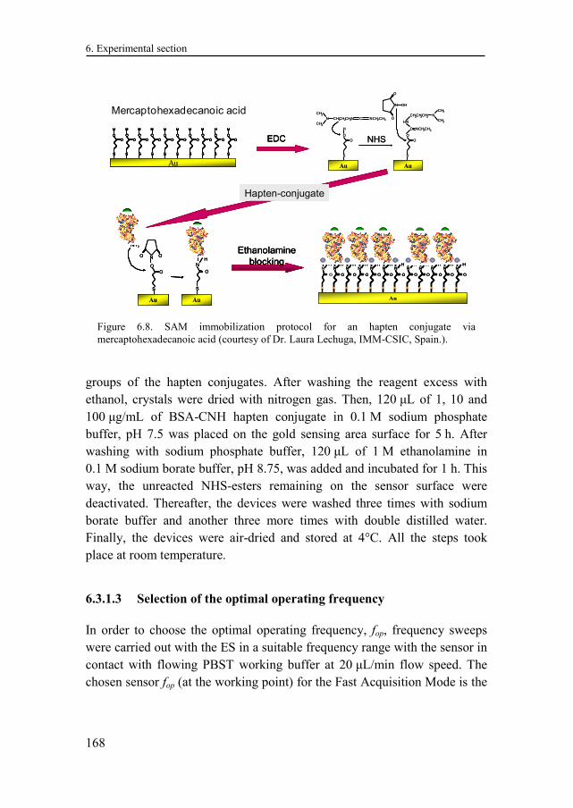
6. Experimental section
168
groups of the hapten conjugates. After washing the reagent excess with ethanol, crystals were dried with nitrogen gas. Then, 120 µL of 1, 10 and 100 µg/mL of BSA-CNH hapten conjugate in 0.1 M sodium phosphate buffer, pH 7.5 was placed on the gold sensing area surface for 5 h. After washing with sodium phosphate buffer, 120 µL of 1 M ethanolamine in 0.1 M sodium borate buffer, pH 8.75, was added and incubated for 1 h. This way, the unreacted NHS-esters remaining on the sensor surface were deactivated. Thereafter, the devices were washed three times with sodium borate buffer and another three more times with double distilled water. Finally, the devices were air-dried and stored at 4°C. All the steps took place at room temperature.
6.3.1.3 Selection of the optimal operating frequency
In order to choose the optimal operating frequency, fop, frequency sweeps were carried out with the ES in a suitable frequency range with the sensor in contact with flowing PBST working buffer at 20 µL/min flow speed. The chosen sensor fop (at the working point) for the Fast Acquisition Mode is the
Figure 6.8. SAM immobilization protocol for an hapten conjugate via mercaptohexadecanoic acid (courtesy of Dr. Laura Lechuga, IMM-CSIC, Spain.).
NHS
N CH2CH2CH2N C NCH 2CH3
CH3
CH3
S
O
O
H
S
O
O
C
HN
CH2CH2CH2 N
CH3
CH3
NCH2CH3
O
O
N OH
Au Au
S
O
O
O ON
NH 2
N
O
S
H
AuAu
Mercaptoundecanoic
or Thioctic acid
AuS
O
O
H
S
O
O
H
S
O
O
H
S
O
O
H
S
O
O
H
S
O
O
H
S
O
O
H
S
O
O
H
S
O
O
H
S
O
O
H
S
O
O
H
S
O
O
H
S
O
O
H
S
O
O
H
S
O
O
H
S
O
O
H
S
O
O
H
S
O
O
H
S
O
O
H
S
O
O
H
N
O
S
H
Au
N
O
S
HN
O
S
HN
O
S
HN
O
S
HN
O
S
HN
O
S
HN
O
S
HN
O
S
HN
O
S
HN
O
S
HN
O
S
HN
O
S
HN
O
S
HN
O
S
HN
O
S
HN
O
S
HN
O
S
HN
O
S
HN
O
S
HN
O
S
HN
O
S
HN
O
S
H
EDC
Ethanolamine
blocking
Hapten-conjugate
NHS
N CH2CH2CH2N C NCH 2CH3
CH3
CH3
S
O
O
H
S
O
O
C
HN
CH2CH2CH2 N
CH3
CH3
NCH2CH3
O
O
N OH
Au Au
S
O
O
O ON
NH 2
N
O
S
H
AuAu
S
O
O
O ON
NH 2
N
O
S
H
AuAu
Mercaptoundecanoic
or Thioctic acid
AuS
O
O
H
S
O
O
H
S
O
O
H
S
O
O
H
S
O
O
H
S
O
O
H
S
O
O
H
S
O
O
H
S
O
O
H
S
O
O
H
S
O
O
H
S
O
O
H
S
O
O
H
S
O
O
H
S
O
O
H
S
O
O
H
S
O
O
H
S
O
O
H
S
O
O
H
S
O
O
H
Mercaptoundecanoic
or Thioctic acid
AuS
O
O
H
S
O
O
H
S
O
O
H
S
O
O
H
S
O
O
H
S
O
O
H
S
O
O
H
S
O
O
H
S
O
O
H
S
O
O
H
S
O
O
H
S
O
O
H
S
O
O
H
S
O
O
H
S
O
O
H
S
O
O
H
S
O
O
H
S
O
O
H
S
O
O
H
S
O
O
H
N
O
S
H
Au
N
O
S
HN
O
S
HN
O
S
HN
O
S
HN
O
S
HN
O
S
HN
O
S
HN
O
S
HN
O
S
HN
O
S
HN
O
S
HN
O
S
HN
O
S
HN
O
S
HN
O
S
HN
O
S
HN
O
S
HN
O
S
HN
O
S
HN
O
S
HN
O
S
HN
O
S
H
EDCEDC
Ethanolamine
blocking
Ethanolamine
blocking
Hapten-conjugateHapten-conjugate
Mercaptohexadecanoic acid
María Isabel Rocha Gaso
169
one at which the IL is minimum and at which the phase-shift is 0° (see Figure 5.20).
6.3.1.4 Immunoassay format
For small analytes, such as the carbaryl pesticide, immunosensors are usually developed in the competitive inhibition (conjugate-coated) format, with immobilized hapten conjugates and monoclonal antibodies as specific recognition immunoreagents [9,12]. Duet to the fact that the antibody immobilization often leads to impaired regeneration capability and poor immunoassay reproducibility of immunosensors, the conjugate-coated assay format was chosen because of its excellent performance, in terms of stability and reliability. Furthermore, covalent binding via SAM ensures highly ordered protein immobilization, which provides numerous advantages, as the improvement of detection limits, reproducibility and reusability, and prevention of non-specific binding of biomolecules [9].
6.3.1.5 Immunoassay protocol
A complete measurement cycle, including sample injection and regeneration, takes 28 min:
1. 5 min flow of PBST at a flow rate of 20 µL/min to stabilize the baseline signal.
2. Sample injection (350 µL) for 15 min. 3. 4 min regeneration with HCl (0.1 M) and 4 min with PBST at a
flow rate of 250 µL/min.
Following this protocol for different standard solutions of the analyte (carbaryl), a calibration curve can be generated. The calibration
curve is used for determining the concentration of an analyte (the substance to be measured) in an unknown sample by relating the unknown to a set of standard samples of known concentration. Next the procedure to obtain the standard calibration curves of this Thesis is described.
6. Experimental section
170
6.3.1.6 Standard calibration curves
To obtain the calibration curve, a fixed amount of the respective MAb was mixed with standard solutions of carbaryl analyte, and the mixture was injected over the sensor surface as follows:
• Standard solutions of carbaryl, in the range of 10−4 to 2×10³ µg/L, were prepared by serial dilutions in PBS and stored at −20°C in dark vials.
• The standards (180 µL) were mixed with fixed concentrations of LIB-CNH45 MAb (180 µL).
• Analyte–antibody solutions were incubated for 1 h at room temperature and then injected and brought onto the sensor surface as described in the immunoassay protocol (Section 6.3.4.1).
The phase-shift (uφ) and amplitude (uA) of the LW biosensor was monitored in real-time as the binding between free antibody and the immobilized conjugate took place. Regeneration of the functionalized surface was accomplished with 0.1M hydrochloric acid (HCl) to break the antibody–hapten conjugate association. When the antibody binds onto the sensing area, an increment of the mass in this area is produced. This change in the physical properties of the layer in contact with the sensor is translated into changes of the characterization system electrical magnitudes; a slight change of IL and a change in the slope of the relation phase-shift versus frequency occur when working at a fixed frequency. This is observed as an increasing or decreasing phase-shift in the ES depending on the selected operating frequency (see Figure 5.20). Since the analyte inhibits antibody binding to the respective immobilized conjugate, increasing concentrations of analyte will decrease the absolute value of the phase-shift increment (∆uφ) of LW sensor response.
Measurements of maximum signal (sample in the absence of analyte) were performed at the beginning and end of every day of assays, as well as in between assays of samples with different carbaryl concentrations. This was done in order to control the evolution of maximum signal during the day and to make sure that the immunosensor was working correctly. At least two assays of maximum signal were run for these control test.
María Isabel Rocha Gaso
171
Standard curves were obtained by plotting the voltage phase-shift (∆uφ) percentage relative to the maximum signal versus the logarithm of analyte concentration. Each point of the calibration curve was run at least three times. Therefore, each experimental point was calculated as the mean value of at least 3 assays and errors were calculated using the standard deviation.
The experimental points were fitted to the four-parameter logistic equation:
( )
( )1B
A Dy D
xC
−= +
+ (6.1)
where A is the asymptotic maximum (maximum signal in the absence of analyte, Smax), B is the slope of the curve at the inflection point (related to the analyte concentration C that gives 50% inhibition of Smax, considered the I50) and D is the asymptotic minimum (background signal). These curves were normalized by expressing the voltage phase-shift (∆uφ) provided by each standard concentration as the percentage of the maximum response (maximum signal, Smax = 100%) in the absence of analyte (∆u0); that is to say, 100·∆uφ/∆uφ0.
Therefore, from the fitting of the experimental points to Eq. (6.1), the following analytical parameters can be determined:
• The I50 value, which is generally accepted as an estimate of the immunosensor sensitivity.
• The immunosensor limit of detection (LOD) is calculated as the analyte concentration that provides 90% of the maximum signal (I90 value).
• The quantification range is the linear working range in which analyte concentrations produced signals between 80 and 20% of the maximum signal (I80-20).
6.3.1.7 Biosensing system
The same A10 test platform describe in Section 6.2.1 (Figure 6.1) was employed for this experiment. For this experiment, the platform fluidic module was actually used.
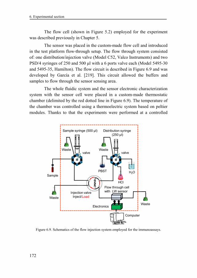
6. Experimental section
172
The flow cell (shown in Figure 5.2) employed for the experiment was described previously in Chapter 5.
The sensor was placed in the custom-made flow cell and introduced in the test platform flow-through setup. The flow through system consisted of: one distribution/injection valve (Model C52, Valco Instruments) and two PSD/4 syringes of 250 and 500 µl with a 6 ports valve each (Model 5495-30 and 5495-35, Hamilton). The flow circuit is described in Figure 6.9 and was developed by García et al. [219]. This circuit allowed the buffers and samples to flow through the sensor sensing area.
The whole fluidic system and the sensor electronic characterization system with the sensor cell were placed in a custom-made thermostatic chamber (delimited by the red dotted line in Figure 6.9). The temperature of the chamber was controlled using a thermoelectric system based on peltier modules. Thanks to that the experiments were performed at a controlled
Figure 6.9. Schematics of the flow injection system employed for the immunoassays.
Sample
Sample syringe (500 µl) Distribution syringe
(250 µl)
Waste
Injection valve
Inject/Load
PBST
HCl
Waste
Waste
H2O
valve valve
Flow through cell
with LW sensor
WasteElectronics
Computer
María Isabel Rocha Gaso
173
temperature of 25°C ± 0.1°C.
The AW-BIO v1.8 software described in Section 6.2.5, run in a remote computer, was employed for controlling the whole system. The software controlled the flow-through system, set the operating frequency, displayed and recorded all the measurements. Thanks to this software, the phase, amplitude and temperature were continuously monitored during the immunoassays.
Next, the results of this experiment are compared with previous developed carbaryl immunosensors based on other technologies where similar or identical immunoreagents and chemicals were used (SPR, HFF-QCM, Traditional QCM and ELISA).
6.3.2 Results and discussion
A real register of a LW carbaryl antibody immunoassay is presented in Figure 6.10, where it is shown the real-time phase-shift signal obtained with the ES during the immunoassay for a concentration of carbaryl antibody. The immunoassay was achieved by immobilizing the hapten-conjugate (BSA–CNH) at 100 µg/mL and injecting carbaryl antibodies (LIB-CNH45 MAb) at 15.625 µg/mL onto the sensor’s surface. The voltage uφ, associated with the phase-shift, increases as soon as the molecular interaction occurs after the sample injection in minute two, due to the adhesion of carbaryl antibodies to the immobilized hapten-conjugate on the sensing area. After 15 minutes of sample injection, the signal is stabilized and the increment in phase-shift with respect to the one at the time of sample injection can be easily calculated: ∆uφ = uφ - uφ0. At the selected operating frequency the slope of the curve phase-shift versus frequency, obtained with the ES, has positive sign (see Figure 5.20). For that reason, when the adhesion of carbaryl antibodies takes place, an increment in the phase-shift is observed and, therefore, the voltage uφ increases. However, if another operating frequency is selected, the same phenomenon can produce a phase-shift decrease, as it occurs in Figure 6.12.
The phase-shift voltage uφ was mainly observed for analyzing the immunosensor, since this signal is primarily related to mass loading of the sensing area, while the IL is more related to viscous losses [223].
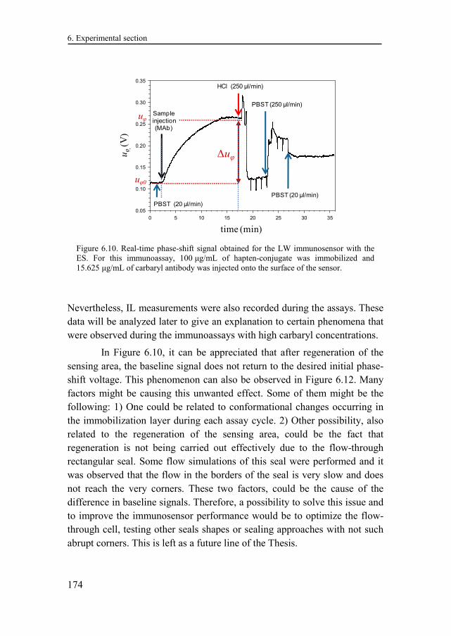
6. Experimental section
174
Nevertheless, IL measurements were also recorded during the assays. These data will be analyzed later to give an explanation to certain phenomena that were observed during the immunoassays with high carbaryl concentrations.
In Figure 6.10, it can be appreciated that after regeneration of the sensing area, the baseline signal does not return to the desired initial phase-shift voltage. This phenomenon can also be observed in Figure 6.12. Many factors might be causing this unwanted effect. Some of them might be the following: 1) One could be related to conformational changes occurring in the immobilization layer during each assay cycle. 2) Other possibility, also related to the regeneration of the sensing area, could be the fact that regeneration is not being carried out effectively due to the flow-through rectangular seal. Some flow simulations of this seal were performed and it was observed that the flow in the borders of the seal is very slow and does not reach the very corners. These two factors, could be the cause of the difference in baseline signals. Therefore, a possibility to solve this issue and to improve the immunosensor performance would be to optimize the flow-through cell, testing other seals shapes or sealing approaches with not such abrupt corners. This is left as a future line of the Thesis.
Figure 6.10. Real-time phase-shift signal obtained for the LW immunosensor with the ES. For this immunoassay, 100 µg/mL of hapten-conjugate was immobilized and 15.625 µg/mL of carbaryl antibody was injected onto the surface of the sensor.
0 5 10 15 20 25 30 35
φ
0.05
0.10
0.15
0.20
0.25
0.30
0.35
Sampleinjection (MAb)
HCl (250 µl/min)
PBST (250 µl/min)
PBST (20 µl/min)
PBST (20 µl/min)
uφ
(V)
time (min)
∆uφ
uφ0
uφ
María Isabel Rocha Gaso
175
Also in relation to the improvement of the LW flow cell, it was observed during the immunosensors experiments that bubbles gathered in the corners of the PDMS rectangular seal when time passed. Furthermore, when a bubble entered through the flow-cell inlet, the bubble remained at the end of the inlet and became bigger during time. This of course affected the measurements, therefore, in the future the flow-cell should be improved in such way that it better allows the free pass of the bubbles generated during the immunoassays.
Another important improvement that can be made is in relation with the contact area of the fabricated LW sensors. Generally, after a certain number of immunoassays, it was observed that the cell probes (spring contacts) damaged the sensor contacts and sometimes the immobilized sensors had to be repaired with a silver conductive paint in order to be used again. In the future, these contacts could be easily reinforced during the fabrication process by applying additional metal layers. In addition, other kind of probes (softer ones) could be placed in the flow cell to avoid an excessive pressure onto the sensors’ contact area.
6.3.2.1 LW carbaryl immunoassay optimization
Low molecular weight compounds, like carbaryl, should be measured using competitive immunoassays. For this type of immunoassays the employed MAb and hapten-conjugate concentrations are crucial to assure the correct competitiveness of the assay and to optimize the LOD and working range of the standard calibration curve. It is well known, that the lower concentration of employed immunoreagents, the better sensitivity and LOD will be achieved in the immunosensor [8,224]. Furthermore, since the immunoreagents are very expensive, the low consume of them will make the sensors more attractive commercially. However, a trade off is required between the low concentration of employed immunoreagents and a sufficient concentration of immunoreagents for being able to distinguish between noise and signal in the employed measurement system.
6. Experimental section
176
Previous studies determined that the conjugate-MAb combination for carbaryl pesticide detection which provides the best assay performance and regeneration capability for piezoelectric sensors is the LIB-CNH45 MAb with BSA–CNH as the immobilized hapten-conjugate [9]. To determine the optimal immunoreagents concentration for the LW immunosensor, several BSA–CNH concentrations (1, 10 and 100 µg/mL) were explored for the conjugate immobilizations. These immobilizations were performed following the protocol technique described in Section 6.3.1.2. MAb solutions of different concentrations in PBS were assayed with a flow rate of 20 µL/min. Under these conditions, maximum phase-shift voltages were produced in 15 min.
Figure 6.11 displays the phase-shift signal change (∆uφ in volts) obtained with LIB-CNH45 MAb assayed in the 1–25 µg/mL concentration range for the different hapten-conjugate concentrations. Triangles represent the values obtained for a hapten-conjugate concentration of 100 µg/mL; circles for a hapten-conjugate concentration of 10 µg/mL; and diamonds for a hapten-conjugate concentration of 1 µg/mL. At least three assays were carried out for each point. As it can be observed in the figure, the influence of MAb concentration on the variation of phase-shift voltage did not
Figure 6.11. Optimization of the carbaryl LW immunosensor assay. Signal variation (∆uφ in 15min at 20 µL/min) as a function of LIB-CNH45 MAb concentration. Triangles for the hapten-conjugate of 100 µg/mL; circles for the hapten-conjugate of 10 µg/mL; and diamonds for the hapten-conjugate of 1 µg/mL.
∆uφ
(mV
)
0 10 20 30
-500
0
500
1000
1500
2000
2500
[BSA-CNH] = 100 ug/mL
[BSA-CNH] = 10 ug/mL
[BSA-CNH] = 1 ug/mL
[MAb LIB-CNH45] (µg/mL)
60%
60%
María Isabel Rocha Gaso
177
reached an asymptotic maximum (plateau value) as normally happens in this dose-responses curves. The MAb concentration that leads to a plateau value should be above 30 µg/mL. Higher concentrations would have been necessary to be tested in order to confirm this. However, such higher concentrations were avoided, since, if used, this technique would stop being competitive compared to other techniques based on HFF-QCM. Moreover, for the explored MAb concentrations the obtained maximum signals were enough to distinguish them from noise and to work comfortably. These are the reasons why higher MAb concentrations were not explored. The assayed values were sufficient to determine the optimal immunoreagents concentrations for a commercially competitive and sensitive immunosensor where low immunoreagents concentrations are sought.
In order to select the hapten-conjugate concentration, the following criteria were considered: the lowest hapten-conjugate concentration which leads to a signal high enough for distinguishing it from the ES noise. In addition, the lower hapten-conjugate concentration is employed the more commercially attractive the sensor will be, since there is a significant cost reduction. Following these criteria, the 100 µg/mL hapten-conjugate concentration was dismissed.
In relation to the optimal MAb concentration, to guarantee a successful competitive immunoassay, a MAb concentration that provides less of the 60% of the obtained plateau value should be used. In our case, since an asymptotic maximum was not reached, as it can be seen in Figure 6.11, the maximum signal obtained for the MAb concentration of 25 µg/mL was used to calcultate the competitive conditions. Thus, a MAb concentration <10 µg/mL was determined as suitable for both selected BSA-CNH concentrations. To provide reasonable signals with a minimum MAb wasting, two preliminary concentrations of 5 µg/mL and 2 µg/mL were chosen for the immunoassays.
Thus, four standard curves for the selected hapten-conjugate concentrations were decided to be developed, as indicated in Table 6.3. It is important to mention that, among the selected concentrations of immunoreagents, the same concentrations of previous works on HFF-QCM for the same application were found [219,221,224]. This was important for comparing both technologies under similar conditions, as it is pursued in the Thesis objectives.
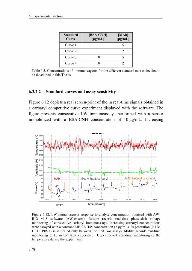
6. Experimental section
178
6.3.2.2 Standard curves and assay sensitivity
Figure 6.12 depicts a real screen-print of the in real-time signals obtained in a carbaryl competitive curve experiment displayed with the software. The figure presents consecutive LW immunoassays performed with a sensor immobilized with a BSA-CNH concentration of 10 µg/mL. Increasing
Figure 6.12. LW immunosensor response to analyte concentration obtained with AW-BIO v1.8 software (AWsensors). Bottom record: real-time phase-shift voltage monitoring of consecutive carbaryl immunoassays. Increasing carbaryl concentrations were assayed with a constant LIB-CNH45 concentration (2 µg/mL). Regeneration (0.1 M HCl + PBST) is indicated only between the first two assays. Middle record: real-time monitoring of IL in the same experiment. Upper record: real-time monitoring of the temperature during the experiment.
MAb + 4µg/L carbarylMAb MAb + 40µg/L carbaryl
HCl
PBST Time (hh:mm)
Pha
se
(V
)A
mp
litud
e (
V)
Te
mpe
ratu
re (
°C)
25.04
24.96
25.00
24.98
25.02
0.775
0.725
0.675
0.625
0.9
0.6
0.3
0.0
-0.3
-0.602:00 02:30 03:00 03:30 04:00 04:30 05:00 05:30 06:00
Standard Curve
[BSA-CNH] (µg/mL)
[MAb] (µg/mL)
Curve 1 1 5
Curve 2 1 2
Curve 3 10 5
Curve 4 10 2
Table 6.3. Concentrations of immunoreagents for the different standard curves decided to be developed in this Thesis.
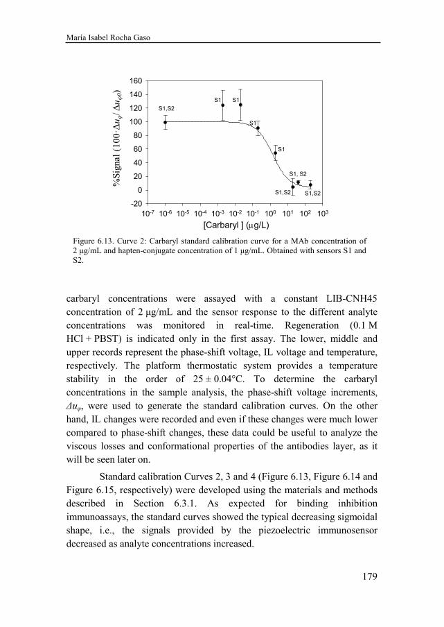
María Isabel Rocha Gaso
179
carbaryl concentrations were assayed with a constant LIB-CNH45 concentration of 2 µg/mL and the sensor response to the different analyte concentrations was monitored in real-time. Regeneration (0.1 M HCl + PBST) is indicated only in the first assay. The lower, middle and upper records represent the phase-shift voltage, IL voltage and temperature, respectively. The platform thermostatic system provides a temperature stability in the order of 25 ± 0.04°C. To determine the carbaryl concentrations in the sample analysis, the phase-shift voltage increments, ∆uφ, were used to generate the standard calibration curves. On the other hand, IL changes were recorded and even if these changes were much lower compared to phase-shift changes, these data could be useful to analyze the viscous losses and conformational properties of the antibodies layer, as it will be seen later on.
Standard calibration Curves 2, 3 and 4 (Figure 6.13, Figure 6.14 and Figure 6.15, respectively) were developed using the materials and methods described in Section 6.3.1. As expected for binding inhibition immunoassays, the standard curves showed the typical decreasing sigmoidal shape, i.e., the signals provided by the piezoelectric immunosensor decreased as analyte concentrations increased.
Figure 6.13. Curve 2: Carbaryl standard calibration curve for a MAb concentration of 2 µg/mL and hapten-conjugate concentration of 1 µg/mL. Obtained with sensors S1 and S2.
%Si
gnal
(10
0·∆
uφ/∆
uφ
0)
10-7 10-6 10-5 10-4 10-3 10-2 10-1 100 101 102 103
-20
0
20
40
60
80
100
120
140
160
LOD = 0.1431 µµµµg/L
I50 = 1.5608 µµµµg/L
I80-20 = 0.3254 - 8.6925µµµµg/L
[Carbaryl ] (µg/L)
S1 S1
S1
S1
S1,S2
S1, S2
S1,S2
S1,S2
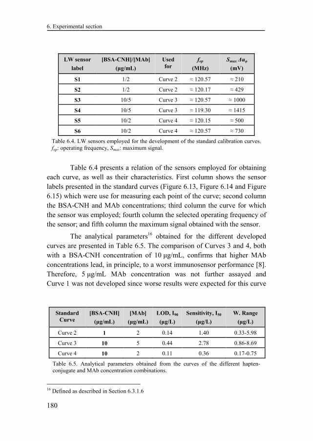
6. Experimental section
180
Table 6.4 presents a relation of the sensors employed for obtaining each curve, as well as their characteristics. First column shows the sensor labels presented in the standard curves (Figure 6.13, Figure 6.14 and Figure 6.15) which were use for measuring each point of the curve; second column the BSA-CNH and MAb concentrations; third column the curve for which the sensor was employed; fourth column the selected operating frequency of the sensor; and fifth column the maximum signal obtained with the sensor.
The analytical parameters16 obtained for the different developed curves are presented in Table 6.5. The comparison of Curves 3 and 4, both with a BSA-CNH concentration of 10 µg/mL, confirms that higher MAb concentrations lead, in principle, to a worst immunosensor performance [8]. Therefore, 5 µg/mL MAb concentration was not further assayed and Curve 1 was not developed since worse results were expected for this curve
16 Defined as described in Section 6.3.1.6
Standard Curve
[BSA-CNH]
(µg/mL)
[MAb]
(µg/mL)
LOD, I90
(µg/L)
Sensitivity, I50
(µg/L)
W. Range
(µg/L)
Curve 2 1 2 0.14 1.40 0.33-5.98
Curve 3 10 5 0.44 2.78 0.86-8.69
Curve 4 10 2 0.11 0.36 0.17-0.75
Table 6.5. Analytical parameters obtained from the curves of the different hapten-conjugate and MAb concentration combinations.
LW sensor
label
[BSA-CNH]/[MAb]
(µg/mL)
Used for
fop
(MHz)
Smax ∆uφ
(mV)
S1 1/2 Curve 2 ≈ 120.57 ≈ 210
S2 1/2 Curve 2 ≈ 120.17 ≈ 429
S3 10/5 Curve 3 ≈ 120.57 ≈ 1000
S4 10/5 Curve 3 ≈ 119.30 ≈ 1415
S5 10/2 Curve 4 ≈ 120.15 ≈ 500
S6 10/2 Curve 4 ≈ 120.57 ≈ 730
Table 6.4. LW sensors employed for the development of the standard calibration curves. fop: operating frequency, Smax: maximum signal.
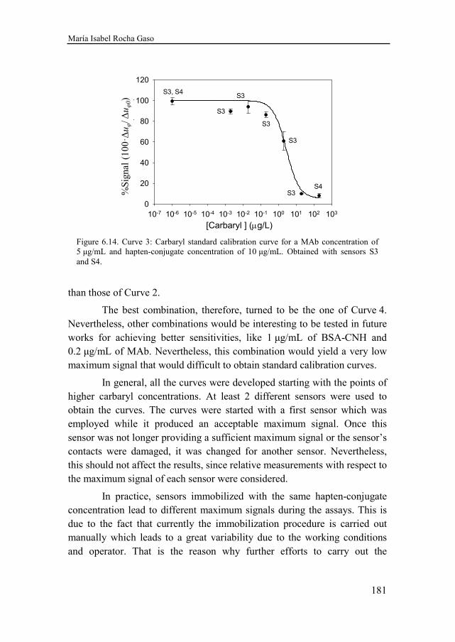
María Isabel Rocha Gaso
181
than those of Curve 2.
The best combination, therefore, turned to be the one of Curve 4. Nevertheless, other combinations would be interesting to be tested in future works for achieving better sensitivities, like 1 µg/mL of BSA-CNH and 0.2 µg/mL of MAb. Nevertheless, this combination would yield a very low maximum signal that would difficult to obtain standard calibration curves.
In general, all the curves were developed starting with the points of higher carbaryl concentrations. At least 2 different sensors were used to obtain the curves. The curves were started with a first sensor which was employed while it produced an acceptable maximum signal. Once this sensor was not longer providing a sufficient maximum signal or the sensor’s contacts were damaged, it was changed for another sensor. Nevertheless, this should not affect the results, since relative measurements with respect to the maximum signal of each sensor were considered.
In practice, sensors immobilized with the same hapten-conjugate concentration lead to different maximum signals during the assays. This is due to the fact that currently the immobilization procedure is carried out manually which leads to a great variability due to the working conditions and operator. That is the reason why further efforts to carry out the
Figure 6.14. Curve 3: Carbaryl standard calibration curve for a MAb concentration of 5 µg/mL and hapten-conjugate concentration of 10 µg/mL. Obtained with sensors S3 and S4.
10-7 10-6 10-5 10-4 10-3 10-2 10-1 100 101 102 103
0
20
40
60
80
100
120
LOD = 0.4386 µµµµg/L
I50 = 3.0562 µµµµg/L
I80-20 = 0.9255 - 11.7178 µµµµg/L
[Carbaryl ] (µg/L)
φφ 0
%Si
gnal
(10
0·∆
uφ/∆
uφ
0)
S3
S3, S4
S4
S3
S3
S3
S3
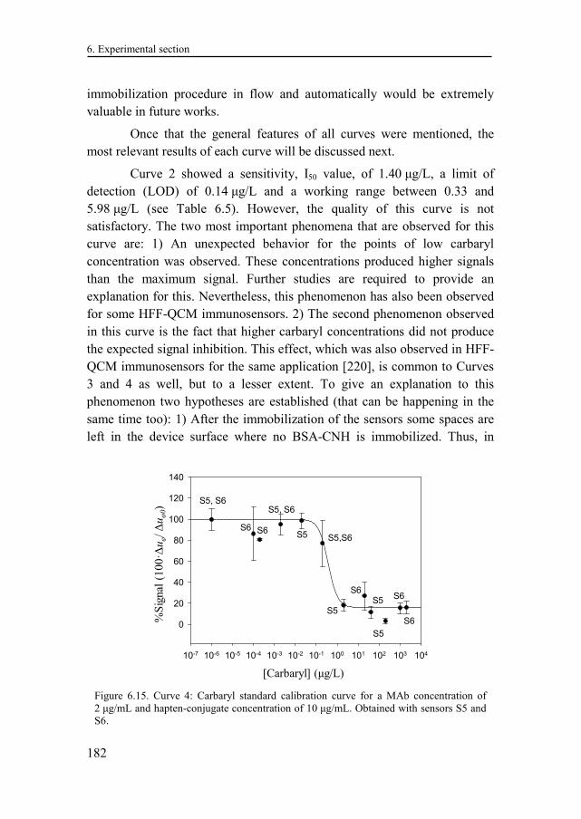
6. Experimental section
182
immobilization procedure in flow and automatically would be extremely valuable in future works.
Once that the general features of all curves were mentioned, the most relevant results of each curve will be discussed next.
Curve 2 showed a sensitivity, I50 value, of 1.40 µg/L, a limit of detection (LOD) of 0.14 µg/L and a working range between 0.33 and 5.98 µg/L (see Table 6.5). However, the quality of this curve is not satisfactory. The two most important phenomena that are observed for this curve are: 1) An unexpected behavior for the points of low carbaryl concentration was observed. These concentrations produced higher signals than the maximum signal. Further studies are required to provide an explanation for this. Nevertheless, this phenomenon has also been observed for some HFF-QCM immunosensors. 2) The second phenomenon observed in this curve is the fact that higher carbaryl concentrations did not produce the expected signal inhibition. This effect, which was also observed in HFF-QCM immunosensors for the same application [220], is common to Curves 3 and 4 as well, but to a lesser extent. To give an explanation to this phenomenon two hypotheses are established (that can be happening in the same time too): 1) After the immobilization of the sensors some spaces are left in the device surface where no BSA-CNH is immobilized. Thus, in
Figure 6.15. Curve 4: Carbaryl standard calibration curve for a MAb concentration of 2 µg/mL and hapten-conjugate concentration of 10 µg/mL. Obtained with sensors S5 and S6.
%S
igna
l (1
00·∆
uφ/∆
uφ
0)
[Carbaryl] (µg/L)
10-7 10-6 10-5 10-4 10-3 10-2 10-1 100 101 102 103 104
0
20
40
60
80
100
120
140
S5
S5
S6S6
S6S5
S5,S6S5
S5, S6
S6S6
S5, S6
María Isabel Rocha Gaso
183
these spaces antibodies can be trapped in a non-specific way producing a change in the phase-shift voltage signal. This phenomenon, might occur for all carbaryl concentrations. When the maximum signal that is used to calculate the relative measurements is lower, this effect is seen as stronger while actually it is not. 2) Another possible explanation of this phenomenon is that a high viscosity of the sample medium is produced when mixing the sample with high carbaryl concentrations. In the same way than hypothesis 1), this becomes an issue when the maximum signal is lower.
In order to check the veracity of hypothesis 1) a change in the previous established protocol was tested passing a 0.1% BSA solution with PBST through the sensor surface before injecting the sample with a high carbaryl concentration (200 µg/L). This was expected to block the empty spaces in the absence of hapten-conjugate in the immobilization layer avoiding non-specific interactions. The result was that BSA-PBST diminished this effect. For that reason, as a future work of the Thesis it is suggested to change the immunoassays protocol using BSA-PBST as the working buffer solution instead of only PBST. However, this change in protocol did not completely solved the problem, thus, hypothesis 2) might also being playing a role. This will be treated with more detail when discussing Curve 4.
Curve 3 showed a sensitivity value of 2.78 µg/L, a LOD of 0.44 µg/L and working range between 0.86 and 8.69 µg/L, as summarized in Table 6.5. In this curve, high carbaryl concentrations produced a better inhibition (near 100%) if compared with Curve 2. The reason is that, even if the viscous effect (in absolute value) is the same than the one for Curve 2, the relative measurement is lower due to a higher maximum signal (see Table 6.4).
Curve 4 showed the best analytical performance. In this curve more points were assayed with carbaryl standards in the 1×10⁻⁴ to 2×10³ µg/L range to better define the curve. The sensitivity value was of 0.36 µg/L, the LOD was 0.11 µg/L and the quantification range was between 0.17 and 0.75 µg/L (see Table 6.5). For this curve, the points of high concentrations of carbaryl (1000 µg/L and 2000 µg/L) were performed using 0.1% BSA solution with PBST as the working buffer, to obtain a better inhibition. With the purpose of analyzing the viscoelastic behavior of the immunosensor’s
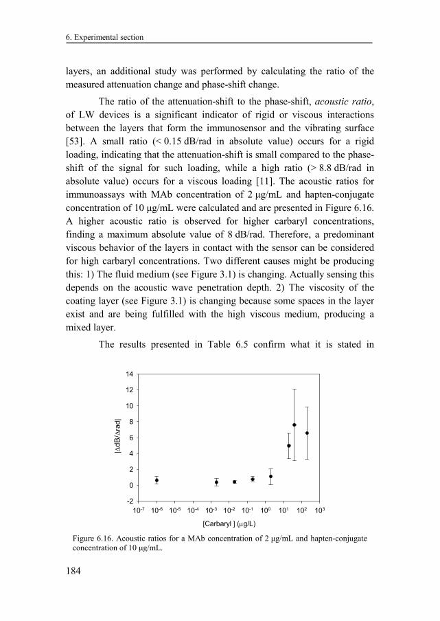
6. Experimental section
184
layers, an additional study was performed by calculating the ratio of the measured attenuation change and phase-shift change.
The ratio of the attenuation-shift to the phase-shift, acoustic ratio, of LW devices is a significant indicator of rigid or viscous interactions between the layers that form the immunosensor and the vibrating surface [53]. A small ratio (< 0.15 dB/rad in absolute value) occurs for a rigid loading, indicating that the attenuation-shift is small compared to the phase-shift of the signal for such loading, while a high ratio (> 8.8 dB/rad in absolute value) occurs for a viscous loading [11]. The acoustic ratios for immunoassays with MAb concentration of 2 µg/mL and hapten-conjugate concentration of 10 µg/mL were calculated and are presented in Figure 6.16. A higher acoustic ratio is observed for higher carbaryl concentrations, finding a maximum absolute value of 8 dB/rad. Therefore, a predominant viscous behavior of the layers in contact with the sensor can be considered for high carbaryl concentrations. Two different causes might be producing this: 1) The fluid medium (see Figure 3.1) is changing. Actually sensing this depends on the acoustic wave penetration depth. 2) The viscosity of the coating layer (see Figure 3.1) is changing because some spaces in the layer exist and are being fulfilled with the high viscous medium, producing a mixed layer.
The results presented in Table 6.5 confirm what it is stated in
Figure 6.16. Acoustic ratios for a MAb concentration of 2 µg/mL and hapten-conjugate concentration of 10 µg/mL.
[Carbaryl ] (µg/L)
10-7 10-6 10-5 10-4 10-3 10-2 10-1 100 101 102 103
-2
0
2
4
6
8
10
12
14
|∆dB
/∆ra
d|
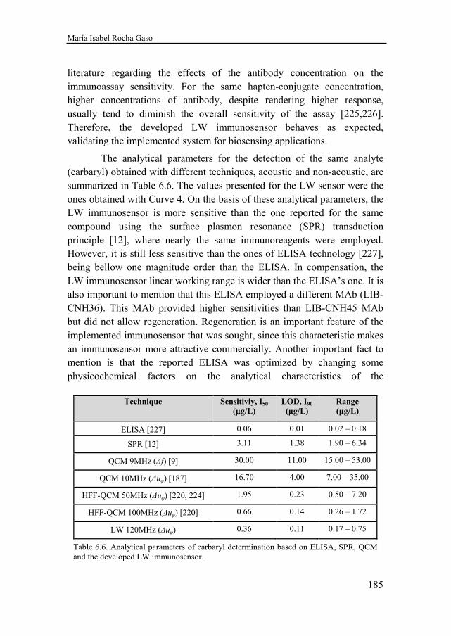
María Isabel Rocha Gaso
185
literature regarding the effects of the antibody concentration on the immunoassay sensitivity. For the same hapten-conjugate concentration, higher concentrations of antibody, despite rendering higher response, usually tend to diminish the overall sensitivity of the assay [225,226]. Therefore, the developed LW immunosensor behaves as expected, validating the implemented system for biosensing applications.
The analytical parameters for the detection of the same analyte (carbaryl) obtained with different techniques, acoustic and non-acoustic, are summarized in Table 6.6. The values presented for the LW sensor were the ones obtained with Curve 4. On the basis of these analytical parameters, the LW immunosensor is more sensitive than the one reported for the same compound using the surface plasmon resonance (SPR) transduction principle [12], where nearly the same immunoreagents were employed. However, it is still less sensitive than the ones of ELISA technology [227], being bellow one magnitude order than the ELISA. In compensation, the LW immunosensor linear working range is wider than the ELISA’s one. It is also important to mention that this ELISA employed a different MAb (LIB-CNH36). This MAb provided higher sensitivities than LIB-CNH45 MAb but did not allow regeneration. Regeneration is an important feature of the implemented immunosensor that was sought, since this characteristic makes an immunosensor more attractive commercially. Another important fact to mention is that the reported ELISA was optimized by changing some physicochemical factors on the analytical characteristics of the
Technique Sensitiviy, I50 (µg/L)
LOD, I90 (µg/L)
Range (µg/L)
ELISA [227] 0.06 0.01 0.02 – 0.18
SPR [12] 3.11 1.38 1.90 – 6.34
QCM 9MHz (∆f) [9] 30.00 11.00 15.00 – 53.00
QCM 10MHz (∆uφ) [187] 16.70 4.00 7.00 – 35.00
HFF-QCM 50MHz (∆uφ) [220, 224] 1.95 0.23 0.50 – 7.20
HFF-QCM 100MHz (∆uφ) [220] 0.66 0.14 0.26 – 1.72
LW 120MHz (∆uφ) 0.36 0.11 0.17 – 0.75
Table 6.6. Analytical parameters of carbaryl determination based on ELISA, SPR, QCM and the developed LW immunosensor.
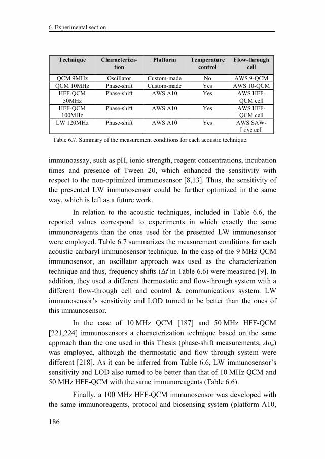
6. Experimental section
186
immunoassay, such as pH, ionic strength, reagent concentrations, incubation times and presence of Tween 20, which enhanced the sensitivity with respect to the non-optimized immunosensor [8,13]. Thus, the sensitivity of the presented LW immunosensor could be further optimized in the same way, which is left as a future work.
In relation to the acoustic techniques, included in Table 6.6, the reported values correspond to experiments in which exactly the same immunoreagents than the ones used for the presented LW immunosensor were employed. Table 6.7 summarizes the measurement conditions for each acoustic carbaryl immunosensor technique. In the case of the 9 MHz QCM immunosensor, an oscillator approach was used as the characterization technique and thus, frequency shifts (∆f in Table 6.6) were measured [9]. In addition, they used a different thermostatic and flow-through system with a different flow-through cell and control & communications system. LW immunosensor’s sensitivity and LOD turned to be better than the ones of this immunosensor.
In the case of 10 MHz QCM [187] and 50 MHz HFF-QCM [221,224] immunosensors a characterization technique based on the same approach than the one used in this Thesis (phase-shift measurements, ∆uφ) was employed, although the thermostatic and flow through system were different [218]. As it can be inferred from Table 6.6, LW immunosensor’s sensitivity and LOD also turned to be better than that of 10 MHz QCM and 50 MHz HFF-QCM with the same immunoreagents (Table 6.6).
Finally, a 100 MHz HFF-QCM immunosensor was developed with the same immunoreagents, protocol and biosensing system (platform A10,
Technique Characteriza-tion
Platform Temperature control
Flow-through cell
QCM 9MHz Oscillator Custom-made No AWS 9-QCM QCM 10MHz Phase-shift Custom-made Yes AWS 10-QCM
HFF-QCM 50MHz
Phase-shift AWS A10 Yes AWS HFF-QCM cell
HFF-QCM 100MHz
Phase-shift AWS A10 Yes AWS HFF-QCM cell
LW 120MHz Phase-shift AWS A10 Yes AWS SAW-Love cell
Table 6.7. Summary of the measurement conditions for each acoustic technique.
María Isabel Rocha Gaso
187
AWSensors) than the ones employed for the LW immunosensor [221]. Only the flow-through cell was different. A10 platform offered the possibility of characterizing both technologies HFF-QCM and LW under similar conditions, using the same temperature, flow-through and electronic measurement systems. To our knowledge, this is the only platform capable to allow these conditions, which are required to perform a reliable comparison between different technologies. From the results presented in Table 6.6, it can be seen that the sensitivity and the LOD of the LW immunosensor are in the same order of magnitude than the ones of the 100 MHz HFF-QCM immunosensor.
In general, a high dispersion between LW immunoassay replicates (assays of samples with the same carbaryl concentration) was observed. This could be mainly due to the lack of optimization of the flow-through cell, which prevented an effective regeneration of the sensor’s surface. Therefore, the analytical parameters achieved by the presented LW immunosensor in Curve 4 are preliminary and further assays for the confirmation of these results are required. It is expected that using a more optimized cell and BSA-PBST, as the working buffer, will diminished the dispersion between the measurements in a future. In addition, further optimizations can be implemented to improve the immunosensor performance, such as optimizing some immunoassay physicochemical factors. Nevertheless, the presented preliminary results suggest that in a near future this immunosensor could allow the detection of carbaryl compound in water intended for human consumption at European regulatory levels17. Moreover, as future works, spiked water samples could be tested with the developed immunosensor or an improved version of it.
6.4 LW sensors versus HFF-QCMs
One of the objectives of this Thesis was to establish a comparison between HFF-QCM and LW technologies. This section includes such comparison.
17The European Union has defined the limit concentration allowable in drinking water for each individual pesticide to 0.10 µg/L in order to protect human helth (Drinking water directive 98/83/EC, 1998).
6. Experimental section
188
LW sensors are more physically robust than HFF-QCMs. The last ones break very easily and in order to be able to work efficiently with them a physical support is required [219]. Conversely, LW sensors are more complex to fabricate which increases their cost.
In general, LW sensors’ sensing area is bigger than HFF-QCMs' sensing area. This presents some advantages and disadvantages. The advantage is that the effect of bubbles presence in the sensing area is diminished on the LW immunoassay response. Since the ratio of the bubble's area and the sensor area is lower in LW sensors than in HFF-QCMs, if a small bubble gets into sensing area, it is possible to continue working without significant signal looses. On the other hand, the disadvantage of a bigger sensing area is that a greater time for the stabilization of the base line immunosensor signal is required. In addition, higher concentrations of immobilization immunoreagents are needed to reach an asymptotic maximum in the sensor’s optimization curve (Figure 6.11).
When it comes to array applications, the big size of LW sensors also represents a disadvantage. An array of 50 LW sensors would be bigger than the one of HFF-QCM sensors, which makes it less commercially attractive. However, the integration of a LW sensor with the electronic circuit is possible and simpler thanks to its compatibility with CMOS processes.
Regarding flow-through cells, the LW cell requires a more complex design, since for confining the liquid in the sensing area it is required to interfere in the way of the propagating acoustic wave. This is not the case for HFF-QCM, which makes the cell design less complex. The rectangular shape of LW sensors’ PDMS seals in contrast to round shapes (o-rings) in QCM sensors, also presented a big inconvenient since bubble get trapped in the seal corners.
LW and 100 MHz HFF-QCM immunosensors data show similar trends in the binding kinetics during the immunoassays. The binding of MAb is fast, reversible whit the regeneration step and it shows MAb concentration dependence: the higher the concentration, the higher ∆uφ is obtained.
With respect to immunosensors sensitivity, the developed 120 MHz LW immunosensor is more sensitive than 50 MHz HFF-QCM, mainly
María Isabel Rocha Gaso
189
because of the frequency difference. Furthermore, the LW immunosensor sensitivity is similar to that of 100 MHz HFF-QCM immunosensor.
6.5 Chapter conclusions
In Experiment 1, the values of phase and attenuation obtained for the different glycerol solutions with the electronic characterization system were in good agreement with those obtained with the transmission line model and network analyzer. They also seem to be in agreement with values reported in literature. Hence, it is concluded that the electronic characterization system is proven as valid for LW devices.
Regarding Experiment 2, a LW-based immunosensor for the determination of carbaryl pesticide was developed. This sensor was based on hapten-conjugate immobilization and monoclonal antibodies. The achieved sensitivity (I50 value) and LOD (I90 value) were around 0.36 µg/L
and 0.11 µg/L, respectively. The linear working range (I80-I20) was of 0.17–0.75 µg/L. The developed LW immunosensor was more sensitive than SPR and in the same order than 100 MHz HFF-QCM immunosensors developed for the same analyte under the same conditions. The achieved LOD of this LW immunosensor could allow the determination of carbaryl in water intended for human consumption at European regulatory levels.
The presented results are preliminary and it is necessary to carry out more experiments to confirm them, since a high variability in the immunoassays was observed. It is necessary to further optimize the flow cell for promoting a better regeneration of the sensor surface and to improve the chemicals flow in the sensing area. In spite of that fact, the results point LW sensors as very promising for biosensing applications. Moreover, it can be stated that they do represent an economic alternative to the overpriced optical SPR systems and a significant promise in terms of simplicity of use and portability for on-line analysis.

María Isabel Rocha Gaso
191
7. Final conclusions
During the work of this Thesis, different acoustic techniques for biosensing applications were reviewed as alternatives to traditional QCMs. LW sensors devices were determined to be the most promising and viable option to work with for these applications. Consequently, the state-of-the-art of LW devices for biosensing was provided and a discussion about the current trends and future challenges of these sensors was presented.
Later, in order to start working with updated LW devices, it was necessary to gather all the up-to-date information regarding the design aspects, operation principles and modeling of such devices. Additionally, some design aspects were explored and tested before the fabrication of the final LW devices. All this information was presented in Chapter 3, where at the end we drove the conclusion that the best suited LW devices for the aims of this Thesis was an AT-cut quartz Z’ propagating substrate, aluminum IDTs, SiO2 guiding layer and gold sensing area. The device center frequency was around 100 MHz for being able to compare with 100 MHz HFF-QCM devices. Therefore, the LW device wavelength was selected to be 40 µm. At the end of the chapter, different simulations for modeling the behavior of the selected device were performed previously to its fabrication.
Thereafter, in Chapter 4, the device fabrication was explained. Due to microfabrication issues, the achieved SiO2 guiding layer thickness was around 3 µm, far from the guiding layer thickness that theoretically could provide the maximum mass sensitivity (see Table 3.10). The final fabricated devices were characterized and a center frequency around 120 MHz was measured.
Next, in Chapter 5, a flow-cell was designed and implemented in order to be able to work in liquid media with the fabricated device. The custom-made cell did not disturb greatly the sensor response. Also, an
7. Final conclusions
192
electronic characterization system (based in phase and amplitude measurement), previously validated for QCMs, was adapted for the fabricated LW devices. The measurements carried out with the implemented flow-through cell and electronic characterization system were satisfactory for working in liquid media. Such system provides the phase-shift and IL of the LW sensor with a high S/N ratio, it is simple, small, fast and it has a high integration capacity. Nevertheless, the developed characterization system is not reliable for measuring high attenuations, which is not an issue for the final application pursued in this Thesis.
In Chapter 7 some experiments were performed with the aim of validating the contributions of this Thesis as suitable for biosensing applications. The proposed electronic characterization system was proven to be valid for LW devices with the fabricated flow cell in Experiment 1 and a LW-based immunosensor for the determination of carbaryl pesticide was successfully developed in Experiment 2. The sensitivity and LOD achieved with this sensor was around 0.36 µg/L and 0.11 µg/L, respectively. Chapter 6 presents the Materials & Methods employed to carry out these experiments. A conjugate-coated immunoassay format was chosen, since it allows the regeneration of the sensor surface. Hence, competitive assays were performed where the carbaryl analyte competed with the immobilized hapten-conjugate for binding to a fixed and limited amount of antibody in the solution. The regeneration of the immunosensor was possible using hydrochloric acid.
In general, it is concluded that the developments completed during the Thesis are valid for biosensing applications, since the experimental behavior of the developed immunosensors was in accordance to what it is stated in the literature for immunosensor developed under other acoustic and non-acoustic detection technologies. Nevertheless, some bubbles and sensing area regenerating issues occurred during the LW immunoassays experiments. Thus, the flow-through cell and sensors itself can be greatly improved for achieving a better optimization.
The lack of optimization produced a high dispersion in the immunosensor measurements. Thus, the presented sensitivity and LOD values are preliminary and it is necessary to carry out more experiments to confirm them. Nevertheless, the confirmed results should be around this order of magnitude. Hence, at the end of the Thesis, the comparison of LW
María Isabel Rocha Gaso
193
sensor with HFF-QCM under very similar conditions was possible (the same characterization, flow-through and thermostatic systems were used for the same application with identical immunoreagents and assay protocol). LW sensors turned to be as sensitive as HFF-QCMs and a LOD in the same order was obtained.
Based on the different issues experienced during the development of this Thesis the following future works are proposed:
• Investigation on new materials for LW sensors.
• Further efforts are required in order to achieve 3D-FEM simulations able to reproduce real size LW sensors, which do not consume excessive computational resources.
• Increase of the LW sensor guiding layer thickness for a more optimum operation and higher sensitivity.
• Study of reflectors effect on the mass sensitivity of LW sensors.
• Improvement of a LW flow-through cell that better allows the free pass of bubbles and a better flow through the sensing area.
• Enhancement of the LW sensor contacts.
• Optimization of the LW immunosensor for carbaryl detection changing some physicochemical factors, which affect the analytical characteristics of the immunoassay.
• Performing LW immunoassays using BSA-PBST as the working buffer solution to avoid non-specific binding.
• Performing LW immunoassays using lower immunoreagent concentrations.
• LW immunoassay with spiked and real water samples.
• Determination of viscosity contribution on phase-shift and IL LW sensor sensitivity. This two experimental data obtained with the sensor are not enough for extracting the unknown parameters of the coating layer.
• Study of the viscoelastic behavior of the layers in contact with the immunosensor.
• Study the phenomena observed for high and low carbaryl concentrations.
• Flow-through immobilization technique.
7. Final conclusions
194
Summarizing, by means of the work completed in this Thesis, the following objectives were fulfill:
1) A new research line on LW devices for biosensing applications was opened in the GFO research group. Information, materials and methods were gathered in this work that will allow to perform further research on the topic.
2) An optimized LW sensor was designed, modeled and fabricated.
3) A complete microsystem for LW devices was developed, adapting the QCM characterization system and fabricating a flow-through cell for LW sensors.
4) The developments completed for LW sensors were validated with a real immunosensor application were a low molecular weight compound, carbaryl, was detected.
5) The performance of HFF-QCM was compared to that of LW sensors for the same application and under the same conditions.
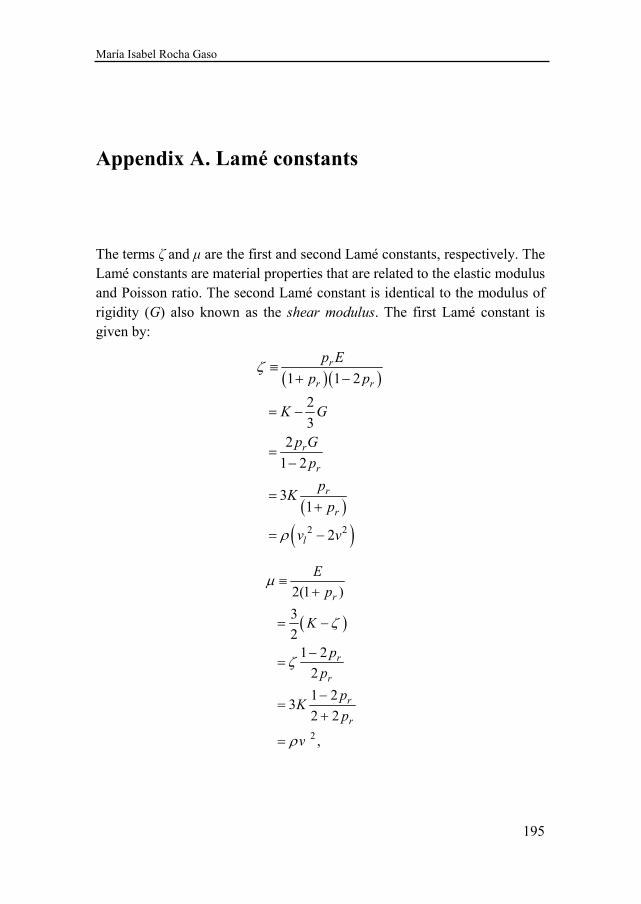
María Isabel Rocha Gaso
195
Appendix A. Lamé constants
The terms ζ and µ are the first and second Lamé constants, respectively. The Lamé constants are material properties that are related to the elastic modulus and Poisson ratio. The second Lamé constant is identical to the modulus of rigidity (G) also known as the shear modulus. The first Lamé constant is given by:
( )( )
( )
( )2 2
1 1 2
2
32
1 2
31
2
r
r r
r
r
r
r
l
p E
p p
K G
p G
p
pK
p
v v
ζ
ρ
≡+ −
= −
=−
=+
= −
( )
2
2(1 )
3
21 2
2
1 23
2 2
,
r
r
r
r
r
E
p
K
p
p
pK
p
v
µ
ζ
ζ
ρ
≡+
= −
−=
−=
+
=
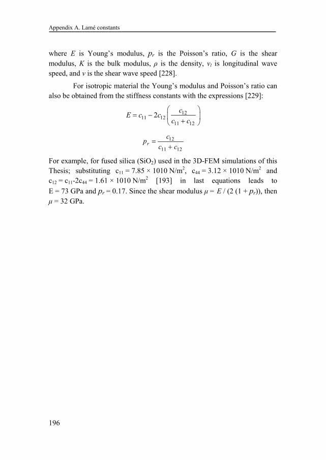
Appendix A. Lamé constants
196
where E is Young’s modulus, pr is the Poisson’s ratio, G is the shear modulus, K is the bulk modulus, ρ is the density, vl is longitudinal wave speed, and v is the shear wave speed [228].
For isotropic material the Young’s modulus and Poisson’s ratio can also be obtained from the stiffness constants with the expressions [229]:
1211 12
11 12
2c
E c cc c
= −
+
12
11 12r
cp
c c=
+
For example, for fused silica (SiO2) used in the 3D-FEM simulations of this Thesis; substituting c11 = 7.85 × 10¹⁰ N/m2, c44 = 3.12 × 10¹⁰ N/m2 and c12 = c11-2c44 = 1.61 × 10¹⁰ N/m2 [193] in last equations leads to
E = 73 GPa and pr = 0.17. Since the shear modulus µ = E / (2 (1 + pr)), then µ = 32 GPa.
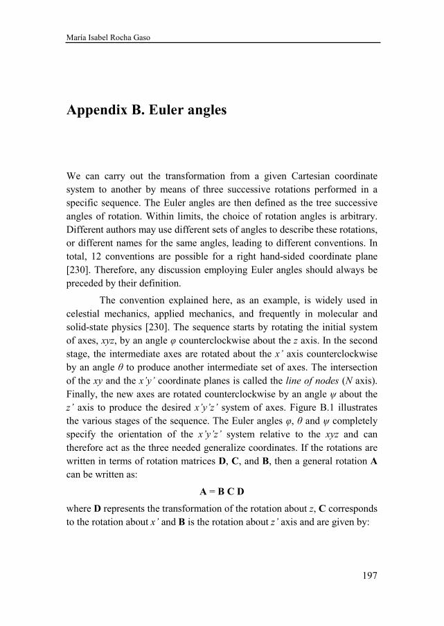
María Isabel Rocha Gaso
197
Appendix B. Euler angles
We can carry out the transformation from a given Cartesian coordinate system to another by means of three successive rotations performed in a specific sequence. The Euler angles are then defined as the tree successive angles of rotation. Within limits, the choice of rotation angles is arbitrary. Different authors may use different sets of angles to describe these rotations, or different names for the same angles, leading to different conventions. In total, 12 conventions are possible for a right hand-sided coordinate plane [230]. Therefore, any discussion employing Euler angles should always be preceded by their definition.
The convention explained here, as an example, is widely used in celestial mechanics, applied mechanics, and frequently in molecular and solid-state physics [230]. The sequence starts by rotating the initial system of axes, xyz, by an angle φ counterclockwise about the z axis. In the second stage, the intermediate axes are rotated about the x’ axis counterclockwise by an angle θ to produce another intermediate set of axes. The intersection of the xy and the x’y’ coordinate planes is called the line of nodes (N axis). Finally, the new axes are rotated counterclockwise by an angle ψ about the z’ axis to produce the desired x’y’z’ system of axes. Figure B.1 illustrates the various stages of the sequence. The Euler angles φ, θ and ψ completely specify the orientation of the x’y’z’ system relative to the xyz and can therefore act as the three needed generalize coordinates. If the rotations are written in terms of rotation matrices D, C, and B, then a general rotation A can be written as:
A = B C D
where D represents the transformation of the rotation about z, C corresponds to the rotation about x’ and B is the rotation about z’ axis and are given by:
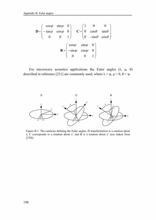
Appendix B. Euler angles
198
cos sin 0
sin cos 0
0 0 1
ϕ ϕϕ ϕ
= −
D
1 0 0
0 cos sin
0 sin cos
θ θθ θ
= −
C
cos sin 0
sin cos 0
0 0 1
ψ ψψ ψ
= −
B
For microwave acoustics applications the Euler angles (λ, µ, θ) described in reference [231] are commonly used, where λ = φ, µ = θ, θ = ψ.
Figure B.1. The rotations defining the Euler angles. D transformation is a rotation about z, C corresponds to a rotation about x’ and B is a rotation about z’ axis (taken from [230]).
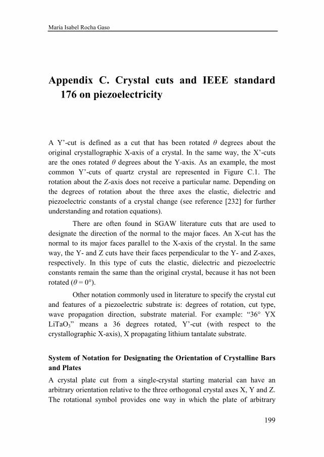
María Isabel Rocha Gaso
199
Appendix C. Crystal cuts and IEEE standard
176 on piezoelectricity
A Y’-cut is defined as a cut that has been rotated θ degrees about the original crystallographic X-axis of a crystal. In the same way, the X’-cuts are the ones rotated θ degrees about the Y-axis. As an example, the most common Y’-cuts of quartz crystal are represented in Figure C.1. The rotation about the Z-axis does not receive a particular name. Depending on the degrees of rotation about the three axes the elastic, dielectric and piezoelectric constants of a crystal change (see reference [232] for further understanding and rotation equations).
There are often found in SGAW literature cuts that are used to designate the direction of the normal to the major faces. An X-cut has the normal to its major faces parallel to the X-axis of the crystal. In the same way, the Y- and Z cuts have their faces perpendicular to the Y- and Z-axes, respectively. In this type of cuts the elastic, dielectric and piezoelectric constants remain the same than the original crystal, because it has not been rotated (θ = 0°).
Other notation commonly used in literature to specify the crystal cut and features of a piezoelectric substrate is: degrees of rotation, cut type, wave propagation direction, substrate material. For example: “36° YX LiTaO3” means a 36 degrees rotated, Y’-cut (with respect to the crystallographic X-axis), X propagating lithium tantalate substrate.
System of Notation for Designating the Orientation of Crystalline Bars
and Plates
A crystal plate cut from a single-crystal starting material can have an arbitrary orientation relative to the three orthogonal crystal axes X, Y and Z. The rotational symbol provides one way in which the plate of arbitrary
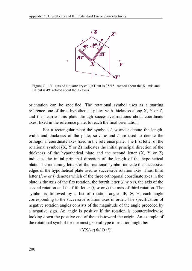
Appendix C. Crystal cuts and IEEE standard 176 on piezoelectricity
200
orientation can be specified. The rotational symbol uses as a starting reference one of three hypothetical plates with thickness along X, Y or Z, and then carries this plate through successive rotations about coordinate axes, fixed in the reference plate, to reach the final orientation.
For a rectangular plate the symbols l, w and t denote the length, width and thickness of the plate; so l, w and t are used to denote the orthogonal coordinate axes fixed in the reference plate. The first letter of the rotational symbol (X, Y or Z) indicates the initial principal direction of the thickness of the hypothetical plate and the second letter (X, Y or Z) indicates the initial principal direction of the length of the hypothetical plate. The remaining letters of the rotational symbol indicate the successive edges of the hypothetical plate used as successive rotation axes. Thus, third letter (l, w or t) denotes which of the three orthogonal coordinate axes in the plate is the axis of the firs rotation, the fourth letter (l, w o t), the axis of the second rotation and the fifth letter (l, w or t) the axis of third rotation. The symbol is followed by a list of rotation angles Φ, Θ, Ψ, each angle corresponding to the successive rotation axes in order. The specification of negative rotation angles consists of the magnitude of the angle preceded by a negative sign. An angle is positive if the rotation is counterclockwise looking down the positive end of the axis toward the origin. An example of the rotational symbol for the most general type of rotation might be:
(YXlwt) Φ/ Θ / Ψ
Figure C.1. Y’-cuts of a quartz crystal (AT cut is 35°15’ rotated about the X- axis and BT cut is 49° rotated about the X- axis).
Z’
Y’
X
Z’
Y’
X
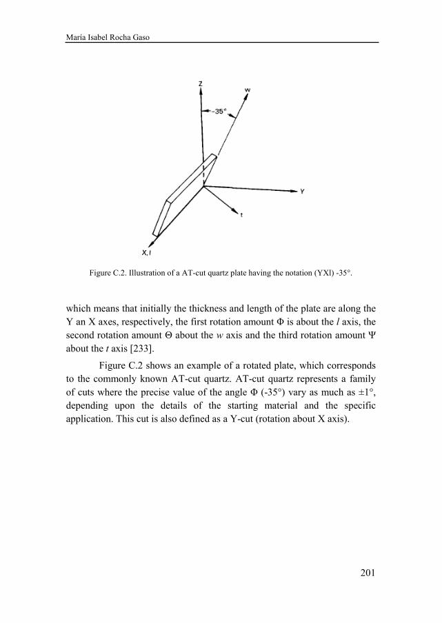
María Isabel Rocha Gaso
201
which means that initially the thickness and length of the plate are along the Y an X axes, respectively, the first rotation amount Φ is about the l axis, the second rotation amount Θ about the w axis and the third rotation amount Ψ about the t axis [233].
Figure C.2 shows an example of a rotated plate, which corresponds to the commonly known AT-cut quartz. AT-cut quartz represents a family of cuts where the precise value of the angle Φ (-35°) vary as much as ±1°, depending upon the details of the starting material and the specific application. This cut is also defined as a Y-cut (rotation about X axis).
Figure C.2. Illustration of a AT-cut quartz plate having the notation (YXl) -35°.

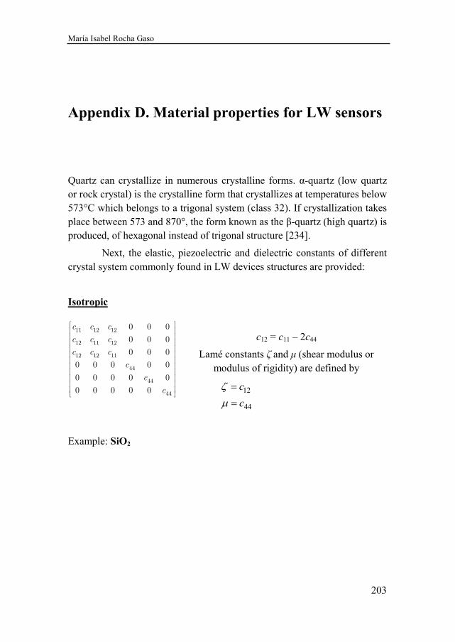
María Isabel Rocha Gaso
203
Appendix D. Material properties for LW sensors
Quartz can crystallize in numerous crystalline forms. α-quartz (low quartz or rock crystal) is the crystalline form that crystallizes at temperatures below 573°C which belongs to a trigonal system (class 32). If crystallization takes place between 573 and 870°, the form known as the β-quartz (high quartz) is produced, of hexagonal instead of trigonal structure [234].
Next, the elastic, piezoelectric and dielectric constants of different crystal system commonly found in LW devices structures are provided:
Isotropic
c12 = c11 – 2c44
Lamé constants ζ and µ (shear modulus or modulus of rigidity) are defined by
12
44
c
c
ζ
µ
=
=
Example: SiO2
11 12 12
12 11 12
12 12 11
44
44
44
0 0 0
0 0 0
0 0 0
0 0 0 0 0
0 0 0 0 0
0 0 0 0 0
c c c
c c c
c c c
c
c
c
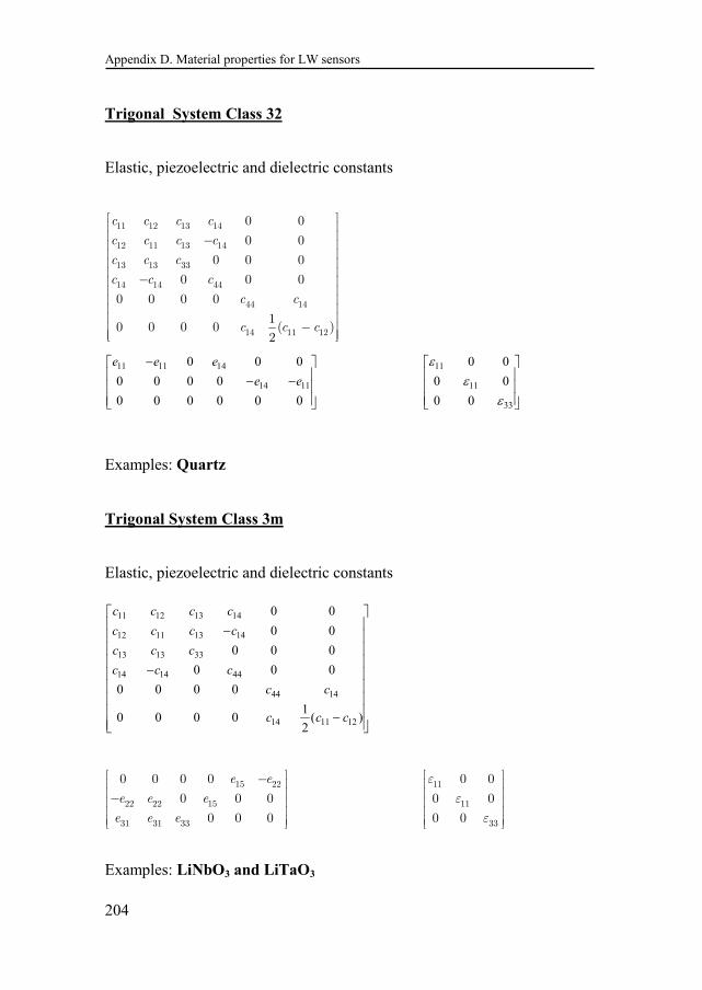
Appendix D. Material properties for LW sensors
204
Trigonal System Class 32
Elastic, piezoelectric and dielectric constants
Examples: Quartz
Trigonal System Class 3m
Elastic, piezoelectric and dielectric constants
Examples: LiNbO3 and LiTaO3
11 12 13 14
12 11 13 14
13 13 33
14 14 44
44 14
14 11 12
0 0
0 0
0 0 0
0 0 0
0 0 0 0
10 0 0 0 ( )
2
c c c c
c c c c
c c c
c c c
c c
c c c
−
−
−
11 11 14
14 11
0 0 0
0 0 0 0
0 0 0 0 0 0
e e e
e e
− − −
11
11
33
0 0
0 0
0 0
εε
ε
11 12 13 14
12 11 13 14
13 13 33
14 14 44
44 14
14 11 12
0 0
0 0
0 0 0
0 0 0
0 0 0 0
10 0 0 0 ( )
2
c c c c
c c c c
c c c
c c c
c c
c c c
−
− −
15 22
22 22 15
31 31 33
0 0 0 0
0 0 0
0 0 0
e e
e e e
e e e
− −
11
11
33
0 0
0 0
0 0
ε
ε
ε
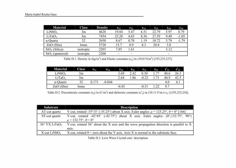
María Isabel Rocha Gaso
205
Material Class Density c11 c12 c13 c33 c44 c14
LiNbO3 3m 4628 19.84 5.47 6.51 22.79 5.97 0.79 LiTaO3 3m 7454 23.28 4.65 8.36 27.59 9.49 -1.05 α-Quartz 32 2650 8.67 0.70 1.19 10.72 5.79 -1.79 ZnO (film) 6mm 5720 15.7 8.9 8.3 20.8 3.8 SiO2 (Silica) isotropic 2203 7.85 1.61 3.12 SiO2 (sputtered) isotropic 2200 - - -
Table D.1. Density in (kg/m3) and Elastic constants (cij) in (1010 N/m2) [193,235-237].
Table D.2. Piezoelectric constants (eij) in (C/m2) and dielectric constants (εsij) in (10-11 F/m ó ε0 ) [193,235,236].
Substrate Description
AT-cut quartz Y-cut, rotated -35°15’ (-35.25°) about X axis. Euler angles: µ = 125.25°, θ = 0° [166] ST-cut quartz Y-cut, rotated -42°45’ (-42.75°) about X axis. Euler angles: (0°,132.75°, 90°)
µ = 132.75°, θ = 0° 36° YX LiTaO3 Y-cut, rotated 36° about the X axis and the wave propagation direction is parallel to X
axis. X-cut LiNbO3 X-cut, rotated θ = zero about the Y axis. Axis X is normal to the substrate face.
Table D.3. Love Wave Crystal cuts’ description.
Material Class e11 e14 e15 e22 e31 e33 εs11 εs
33
LiNbO3 3m 3.69 2.42 0.30 1.77 40.6 26.3 LiTaO3 3m 2.64 1.86 -0.22 1.71 40.9 42.5
α-Quartz 32 0.171 -0.044 4.0 4.1 ZnO (film) 6mm -0.45 -0.51 1.22 9.7
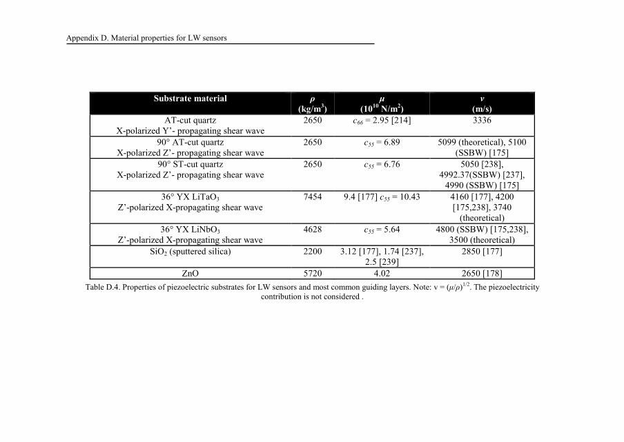
Appendix D. Material properties for LW sensors
206
Table D.4. Properties of piezoelectric substrates for LW sensors and most common guiding layers. Note: v = (µ/ρ)1/2. The piezoelectricity contribution is not considered .
Substrate material ρ
(kg/m3) µ
(1010 N/m2) v
(m/s)
AT-cut quartz X-polarized Y’- propagating shear wave
2650 c66 = 2.95 [214] 3336
90° AT-cut quartz X-polarized Z’- propagating shear wave
2650 c55 = 6.89 5099 (theoretical), 5100 (SSBW) [175]
90° ST-cut quartz X-polarized Z’- propagating shear wave
2650 c55 = 6.76 5050 [238], 4992.37(SSBW) [237],
4990 (SSBW) [175] 36° YX LiTaO3
Z’-polarized X-propagating shear wave 7454 9.4 [177] c55 = 10.43 4160 [177], 4200
[175,238], 3740 (theoretical)
36° YX LiNbO3 Z’-polarized X-propagating shear wave
4628 c55 = 5.64 4800 (SSBW) [175,238], 3500 (theoretical)
SiO2 (sputtered silica) 2200 3.12 [177], 1.74 [237], 2.5 [239]
2850 [177]
ZnO 5720 4.02 2650 [178]
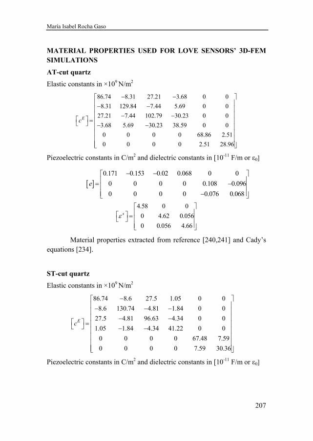
María Isabel Rocha Gaso
207
MATERIAL PROPERTIES USED FOR LOVE SENSORS’ 3D-FEM
SIMULATIONS
AT-cut quartz
Elastic constants in ×109 N/m2
86.74 8.31 27.21 3.68 0 0
8.31 129.84 7.44 5.69 0 0
27.21 7.44 102.79 30.23 0 0
3.68 5.69 30.23 38.59 0 0
0 0 0 0 68.86 2.51
0 0 0 0 2.51 28.96
Ec
− − − − − −
= − −
Piezoelectric constants in C/m2 and dielectric constants in [10-11 F/m or ε0]
[ ]0.171 0.153 0.02 0.068 0 0
0 0 0 0 0.108 0.096
0 0 0 0 0.076 0.068
e
− − = − −
4.58 0 0
0 4.62 0.056
0 0.056 4.66
sε =
Material properties extracted from reference [240,241] and Cady’s
equations [234].
ST-cut quartz
Elastic constants in ×109 N/m2
86.74 8.6 27.5 1.05 0 0
8.6 130.74 4.81 1.84 0 0
27.5 4.81 96.63 4.34 0 0
1.05 1.84 4.34 41.22 0 0
0 0 0 0 67.48 7.59
0 0 0 0 7.59 30.36
Ec
− − − − − −
= − −
Piezoelectric constants in C/m2 and dielectric constants in [10-11 F/m or ε0]
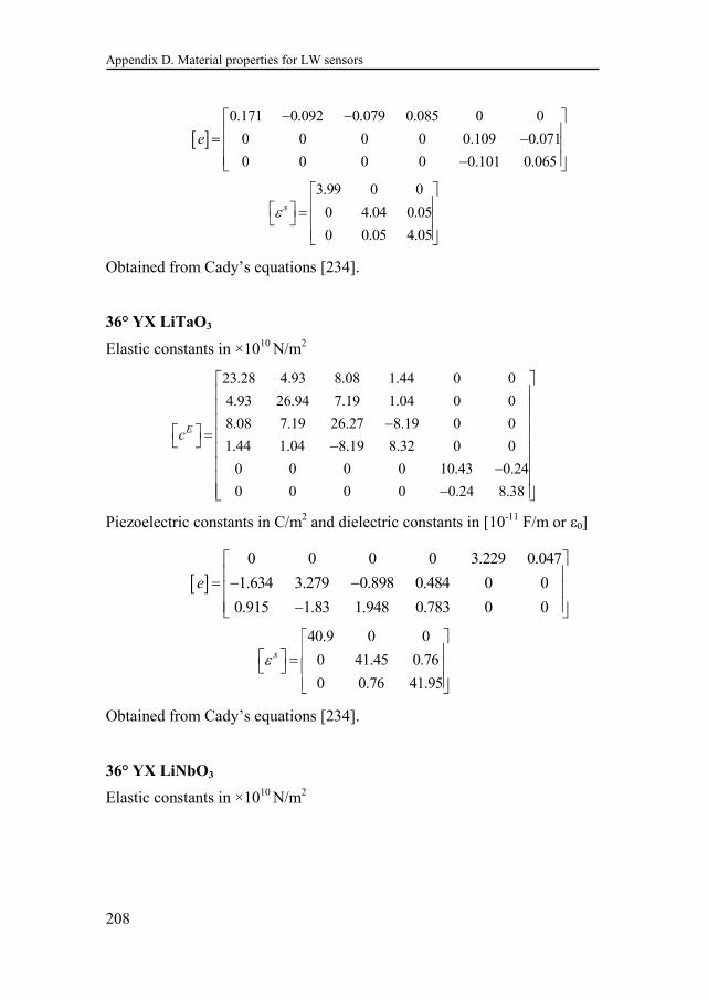
Appendix D. Material properties for LW sensors
208
[ ]0.171 0.092 0.079 0.085 0 0
0 0 0 0 0.109 0.071
0 0 0 0 0.101 0.065
e
− − = − −
3.99 0 0
0 4.04 0.05
0 0.05 4.05
sε =
Obtained from Cady’s equations [234].
36° YX LiTaO3
Elastic constants in ×1010 N/m2
23.28 4.93 8.08 1.44 0 0
4.93 26.94 7.19 1.04 0 0
8.08 7.19 26.27 8.19 0 0
1.44 1.04 8.19 8.32 0 0
0 0 0 0 10.43 0.24
0 0 0 0 0.24 8.38
Ec
−
= − −
−
Piezoelectric constants in C/m2 and dielectric constants in [10-11 F/m or ε0]
[ ]0 0 0 0 3.229 0.047
1.634 3.279 0.898 0.484 0 0
0.915 1.83 1.948 0.783 0 0
e
= − − −
40.9 0 0
0 41.45 0.76
0 0.76 41.95
sε =
Obtained from Cady’s equations [234].
36° YX LiNbO3
Elastic constants in ×1010 N/m2
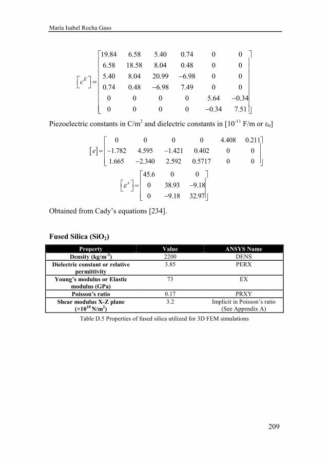
María Isabel Rocha Gaso
209
19.84 6.58 5.40 0.74 0 0
6.58 18.58 8.04 0.48 0 0
5.40 8.04 20.99 6.98 0 0
0.74 0.48 6.98 7.49 0 0
0 0 0 0 5.64 0.34
0 0 0 0 0.34 7.51
Ec
−
= − −
−
Piezoelectric constants in C/m2 and dielectric constants in [10-11 F/m or ε0]
[ ]0 0 0 0 4.408 0.211
1.782 4.595 1.421 0.402 0 0
1.665 2.340 2.592 0.5717 0 0
e
= − − −
45.6 0 0
0 38.93 9.18
0 9.18 32.97
sε = − −
Obtained from Cady’s equations [234].
Fused Silica (SiO2)
Property Value ANSYS Name
Density (kg/m-3) 2200 DENS Dielectric constant or relative
permittivity 3.85 PERX
Young’s modulus or Elastic modulus (GPa)
73 EX
Poisson’s ratio 0.17 PRXY Shear modulus X-Z plane
(×1010 N/m2) 3.2 Implicit in Poisson’s ratio
(See Appendix A)
Table D.5 Properties of fused silica utilized for 3D FEM simulations

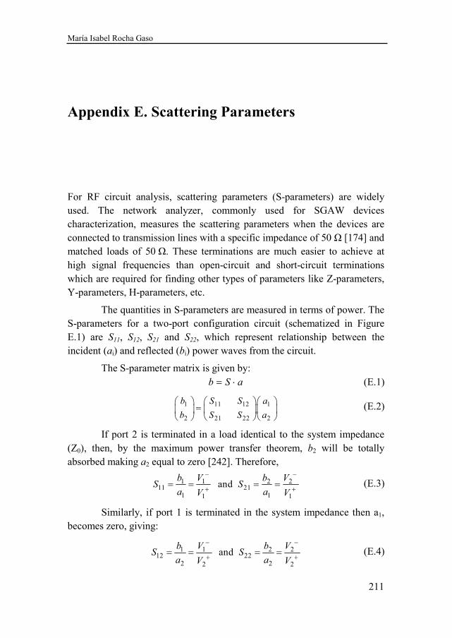
María Isabel Rocha Gaso
211
Appendix E. Scattering Parameters
For RF circuit analysis, scattering parameters (S-parameters) are widely used. The network analyzer, commonly used for SGAW devices characterization, measures the scattering parameters when the devices are connected to transmission lines with a specific impedance of 50 Ω [174] and matched loads of 50 Ω. These terminations are much easier to achieve at high signal frequencies than open-circuit and short-circuit terminations which are required for finding other types of parameters like Z-parameters, Y-parameters, H-parameters, etc.
The quantities in S-parameters are measured in terms of power. The S-parameters for a two-port configuration circuit (schematized in Figure E.1) are S11, S12, S21 and S22, which represent relationship between the incident (ai) and reflected (bi) power waves from the circuit.
The S-parameter matrix is given by: b S a= ⋅ (1.1)(E.1)
1 11 12 1
2 21 22 2
b S S a
b S S a
=
(1.2)(E.2)
If port 2 is terminated in a load identical to the system impedance (Z0), then, by the maximum power transfer theorem, b2 will be totally absorbed making a2 equal to zero [242]. Therefore,
1 1 2 211 21
1 11 1
and b V b V
S Sa aV V
− −
+ += = = = (1.3)(E.3)
Similarly, if port 1 is terminated in the system impedance then a1, becomes zero, giving:
1 1 2 212 22
2 22 2
and b V b V
S Sa aV V
− −
+ += = = = (1.4)(E.4)
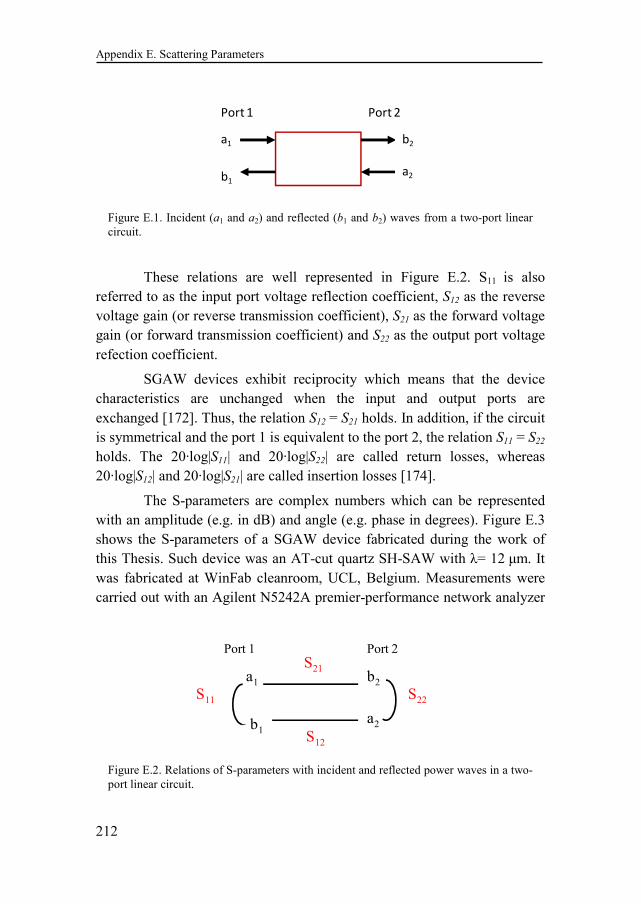
Appendix E. Scattering Parameters
212
These relations are well represented in Figure E.2. S11 is also referred to as the input port voltage reflection coefficient, S12 as the reverse voltage gain (or reverse transmission coefficient), S21 as the forward voltage gain (or forward transmission coefficient) and S22 as the output port voltage refection coefficient.
SGAW devices exhibit reciprocity which means that the device characteristics are unchanged when the input and output ports are exchanged [172]. Thus, the relation S12 = S21 holds. In addition, if the circuit is symmetrical and the port 1 is equivalent to the port 2, the relation S11 = S22 holds. The 20·log|S11| and 20·log|S22| are called return losses, whereas 20·log|S12| and 20·log|S21| are called insertion losses [174].
The S-parameters are complex numbers which can be represented with an amplitude (e.g. in dB) and angle (e.g. phase in degrees). Figure E.3 shows the S-parameters of a SGAW device fabricated during the work of this Thesis. Such device was an AT-cut quartz SH-SAW with λ= 12 µm. It was fabricated at WinFab cleanroom, UCL, Belgium. Measurements were carried out with an Agilent N5242A premier-performance network analyzer
Figure E.2. Relations of S-parameters with incident and reflected power waves in a two-port linear circuit.
Port 1 Port 2
a1 b2
a2
S11 S22
S21
S12
b1
Figure E.1. Incident (a1 and a2) and reflected (b1 and b2) waves from a two-port linear circuit.
b1
a1 b2
a2
Port 1 Port 2
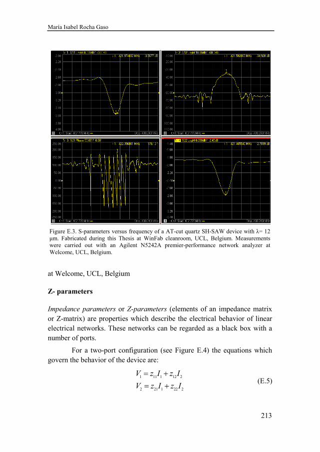
María Isabel Rocha Gaso
213
at Welcome, UCL, Belgium
Z- parameters
Impedance parameters or Z-parameters (elements of an impedance matrix or Z-matrix) are properties which describe the electrical behavior of linear electrical networks. These networks can be regarded as a black box with a number of ports.
For a two-port configuration (see Figure E.4) the equations which govern the behavior of the device are:
1 11 1 12 2
2 21 1 22 2
V z I z I
V z I z I
= +
= + (1.5)(E.5)
Figure E.3. S-parameters versus frequency of a AT-cut quartz SH-SAW device with λ= 12 µm. Fabricated during this Thesis at WinFab cleanroom, UCL, Belgium. Measurements were carried out with an Agilent N5242A premier-performance network analyzer at Welcome, UCL, Belgium.
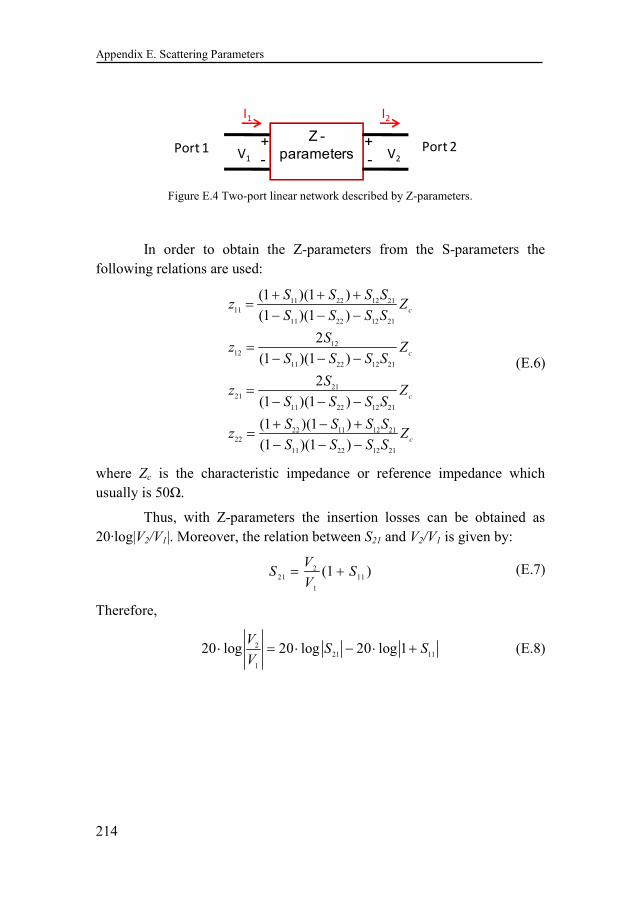
Appendix E. Scattering Parameters
214
In order to obtain the Z-parameters from the S-parameters the following relations are used:
11 22 12 2111
11 22 12 21
1212
11 22 12 21
2121
11 22 12 21
22 11 12 2122
11 22 12 21
(1 )(1 )
(1 )(1 )
2
(1 )(1 )
2
(1 )(1 )
(1 )(1 )
(1 )(1 )
c
c
c
c
S S S Sz Z
S S S S
Sz Z
S S S S
Sz Z
S S S S
S S S Sz Z
S S S S
+ + +=
− − −
=− − −
=− − −
+ − +=
− − −
(1.6)(E.6)
where Zc is the characteristic impedance or reference impedance which usually is 50Ω.
Thus, with Z-parameters the insertion losses can be obtained as 20·log|V2/V1|. Moreover, the relation between S21 and V2/V1 is given by:
221 11
1
(1 )V
S SV
= + (1.7)(E.7)
Therefore,
221 11
1
20 log 20 log 20 log 1V
S SV
⋅ = ⋅ − ⋅ + (1.8)(E.8)
Figure E.4 Two-port linear network described by Z-parameters.
V2V1
I1
Port 1 Port 2
I2
+
-
+
-
Z -
parameters
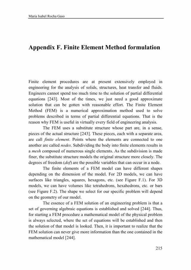
María Isabel Rocha Gaso
215
Appendix F. Finite Element Method formulation
Finite element procedures are at present extensively employed in engineering for the analysis of solids, structures, heat transfer and fluids. Engineers cannot spend too much time to the solution of partial differential equations [243]. Most of the times, we just need a good approximate solution that can be gotten with reasonable effort. The Finite Element Method (FEM) is a numerical approximation method used to solve problems described in terms of partial differential equations. That is the reason why FEM is useful in virtually every field of engineering analysis. The FEM uses a substitute structure whose part are, in a sense, pieces of the actual structure [243]. These pieces, each with a separate area, are call finite element. Points where the elements are connected to one another are called nodes. Subdividing the body into finite elements results in a mesh composed of numerous single elements. As the subdivision is made finer, the substitute structure models the original structure more closely. The degrees of freedom (dof) are the possible variables that can occur in a node. The finite elements of a FEM model can have different shapes depending on the dimension of the model. For 2D models, we can have surfaces like triangles, squares, hexagons, etc. (see Figure F.1). For 3D models, we can have volumes like tetrahedrons, hexahedrons, etc. or bars (see Figure F.2). The shape we select for our specific problem will depend on the geometry of our model. The essence of a FEM solution of an engineering problem is that a set of governing algebraic equations is established and solved [244]. Thus, for starting a FEM procedure a mathematical model of the physical problem is always selected, where the set of equations will be established and then the solution of that model is looked. Then, it is important to realize that the FEM solution can never give more information than the one contained in the mathematical model [244].
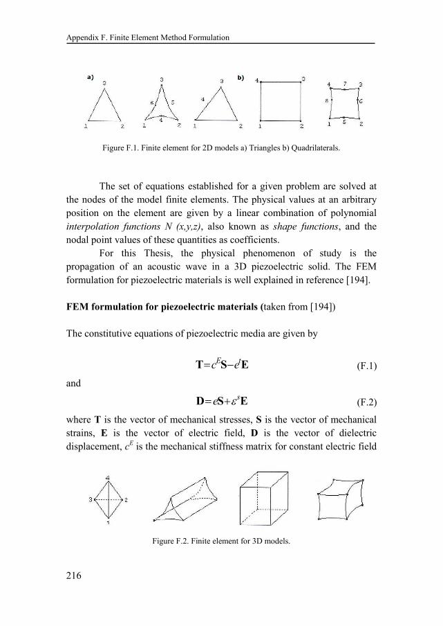
Appendix F. Finite Element Method Formulation
216
The set of equations established for a given problem are solved at the nodes of the model finite elements. The physical values at an arbitrary position on the element are given by a linear combination of polynomial interpolation functions N (x,y,z), also known as shape functions, and the nodal point values of these quantities as coefficients. For this Thesis, the physical phenomenon of study is the propagation of an acoustic wave in a 3D piezoelectric solid. The FEM formulation for piezoelectric materials is well explained in reference [194]. FEM formulation for piezoelectric materials (taken from [194]) The constitutive equations of piezoelectric media are given by
E tc e= −T S E (1.1)(F.1)
and
se ε= +D S E (1.2)(F.2)
where T is the vector of mechanical stresses, S is the vector of mechanical strains, E is the vector of electric field, D is the vector of dielectric displacement, cE is the mechanical stiffness matrix for constant electric field
Figure F.1. Finite element for 2D models a) Triangles b) Quadrilaterals.
Figure F.2. Finite element for 3D models.
María Isabel Rocha Gaso
217
E, εs is the permittivity matrix for constant mechanical strain and e is the piezoelectric matrix.
The electric field E and mechanical strain S are related to the electrical potential Φ and mechanical displacement u, respectively, as follows:
grad= − ΦE (1.3)(F.3)
S Bu= (1.4)(F.4)
where
/ 0 0
0 / 0
0 0 /
/ / 0
0 / /
/ 0 /
x
y
zB
y x
z y
z x
∂ ∂ ∂ ∂ ∂ ∂
= ∂ ∂ ∂ ∂ ∂ ∂ ∂ ∂ ∂ ∂ ∂ ∂
The propagation of acoustic waves in piezoelectric solids is governed by the mechanical equations of motion and Maxwell’s equations for electrical behavior. The elastic behavior of piezoelectric media is governed by Newton’s law:
2
2DivT
u
tρ
∂=
∂ (1.5)(F.5)
Where Div is the divergence of dyadic and ρ is the density of the piezoelectric medium.
The electrical behavior is described by the Maxwell’s equation, considering that piezoelectric media are insulating and have no free volume charge:
0=divD (1.6)(F.6)
Equations F.1 to F.6 constitute a complete set of differential equation, which can be solved with appropriate mechanical and electrical boundary conditions. The mechanical boundary conditions are
Appendix F. Finite Element Method Formulation
218
displacements and forces, whereas electrical boundary conditions are potential and charges.
Hamilton’s variational principle to piezoelectric material gives an equivalent description of the above boundary value problem:
dt 0Eδ =∫ (1.7)(F.7)
The operator δ denotes first-order variation, and the Lagrangian term E is determined by the energies available in the piezoelectric medium
kinetic elastic dielectricE E E E W= − + + (1.8)(F.8)
where, the respective energies are:
2kinetic
elastic
dielectric
1dV
21
' dV2
1' dV
2
E u
E S T
E D E
ρ=
=
=
∫∫∫
∫∫∫
∫∫∫
(1.9)(F.9)
An energy W is generated by external mechanical and electrical excitations, which can be express as follows:
dV dA dAb s s pF F Ft tpW u u q Q= + − Φ + − Φ∑ ∑∫∫∫ ∫∫ ∫∫
(F.10)
(1.10)
where, Fb is the vector of mechanical body forces, Fs is the vector of mechanical surface forces, Fp is the vector of mechanical point forces, qs are the surface charges, and Qp are the point charges.
The system of equations represented from F.1 to F.10, as well as the values of mechanical displacements, forces, electrical potential and charge are solved for at the nodes of all the elements of the FEM model. The values of these mechanical and electrical quantities at an arbitrary position on the element are given by the shape functions N (x,y,z) and the nodal point values of these quantities as coefficients. For an element with n nodes (nodal coordinates: (xi, yi, zi), i = 1, 2,…, n), the continuous displacement function u (x, y, z), can be evaluated from its discrete nodal point vectors as follows:
ˆ( , , ) ( , , ) ( , , )u i i iu x y z N x y z x y z= u (1.11)(F.11)
María Isabel Rocha Gaso
219
where u is a vector of nodal point displacement (order 3n) and Nu is the shape function of interpolation function for displacement. In the same way, other mechanical and electrical quantities are interpolated using appropriate shape functions. Whit the shape functions for displacement Nu and the electric potential NΦ, Equations F.3 and F.4 can be written as:
ˆgrad grad( )ΦE NΦ= − Φ = (1.12)(F.12)
ˆuS Bu BN= = u (1.13)(F.13)
A set of linear differential equations describing one single piezoelectric finite element by substituting shape functions Nx into Equation F.7:
ˆ ˆ ˆ ˆ ˆ ˆ ˆb s pu u u Φ F +F +Fuu uu um d k k Φ+ + + = (1.14)(F.14)
ˆ ˆˆu Φtu s pk k Q QΦ ΦΦ+ = + (1.15)(F.15)
where u , u represent vectors of nodal velocities an accelerations, respectively. The various matrices in the above coupled equations are listed below [245]:
Mechanical stiffness matrix:
dVt Euu u uk B c B= ∫∫∫ (1.16)(F.16)
Mechanical damping matrix:
( ) ( )dV dVe t e t Euu u u u ud N N B c Bα ρ β= +∫∫∫ ∫∫∫ (1.17)(F.17)
Piezoelectric coupling matrix:
dVt tu uk B e BΦ Φ= ∫∫∫ (1.18)(F.18)
Dielectric stiffness matrix:
dVt Sk B BεΦΦ Φ Φ= ∫∫∫ (1.19)(F.19)
Mass matrix:
dVtu um N Nρ= ∫∫∫ (1.20)(F.20)
Mechanical body forces:
Appendix F. Finite Element Method Formulation
220
( )ˆ dVetB u FB BF N N f= ∫∫∫ (1.21)(F.21)
Mechanical surface forces:
( )ˆ dVetS u FS SF N N f= ∫∫∫ (1.22)(F.22)
Mechanical pint forces:
( )ˆ t e
p u pF N F= (1.23)(F.23)
Electrical surface charges:
( )ˆ dAt eS QS sQ N N qΦ= −∫∫ (1.24)(F.24)
Electrical point charges:
( )ˆ t e
p pQ N QΦ=− (1.25)(F.25)
where the following are the forces acting at any element (e): α
(e), β(e)
are the damping coefficients of element (e) ( )e
Bf is the external body force ( )e
Sf is the external surface force
( )epF is the external point force
( )esq is the external surface charge
( )epQ is the external point charge
The magnitudes of the damping matrices depend on the energy dissipation characteristics of the modeled structure. A set of linear differential equations represents the complete finite element mesh of the modeled piezoelectric substrate.
uu uu u B S PMu D u K u K F F FΦ+ + + Φ= + + (1.26)(F.26)
tu S PK u K Q QΦ ΦΦ+ Φ = + (1.27)(F.27)
The quantities in these set of equation are globally assembled field quantities. If the entire mesh is composed of a total of n nodes and the
María Isabel Rocha Gaso
221
model is solved for four degrees of freedom (three displacements and potential), then matrix Equation F.26 will consist of 3*n and Eq. F.27 will consist of n linear differential equation, having in total of 4*n linear equations. The solution to equations F.26 and F.27 yields the mechanical displacements and the electrical potential in piezoelectric media. These set of equations can be solved using various commercially available software packages, such as ANSYS, PZFLEX, ABAQUS, COMSOL, etc.

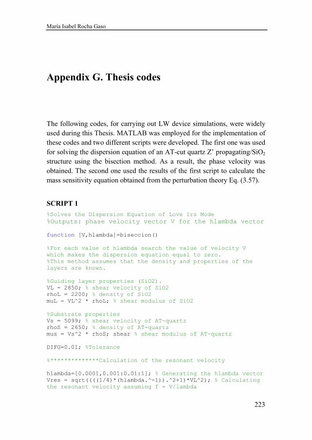
María Isabel Rocha Gaso
223
Appendix G. Thesis codes
The following codes, for carrying out LW device simulations, were widely used during this Thesis. MATLAB was employed for the implementation of these codes and two different scripts were developed. The first one was used for solving the dispersion equation of an AT-cut quartz Z’ propagating/SiO2 structure using the bisection method. As a result, the phase velocity was obtained. The second one used the results of the first script to calculate the mass sensitivity equation obtained from the perturbation theory Eq. (3.57).
SCRIPT 1
%Solves the Dispersion Equation of Love 1rs Mode
%Outputs: phase velocity vector V for the hlambda vector
function [V,hlambda]=biseccion()
%For each value of hlambda search the value of velocity V
which makes the dispersion equation equal to zero.
%This method assumes that the density and properties of the
layers are known.
%Guiding layer properties (SiO2).
VL = 2850; % shear velocity of SiO2
rhoL = 2200; % density of SiO2
muL = VL^2 * rhoL; % shear modulus of SiO2
%Substrate properties
Vs = 5099; % shear velocity of AT-quartz
rhoS = 2650; % density of AT-quartz
mus = Vs^2 * rhoS; shear % shear modulus of AT-quartz
DIFG=0.01; %Tolerance
%**************Calculation of the resonant velocity
hlambda=[0.0001,0.001:0.01:1]; % Generating the hlambda vector
Vres = sqrt((((1/4)*(hlambda.^-1)).^2+1)*VL^2); % Calculating
the resonant velocity assuming f = V/lambda
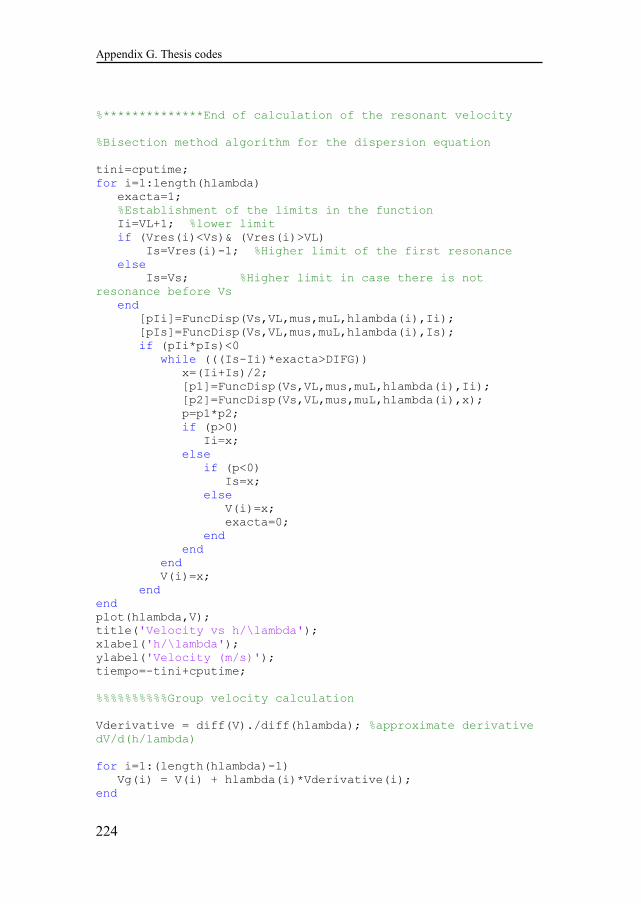
Appendix G. Thesis codes
224
%**************End of calculation of the resonant velocity
%Bisection method algorithm for the dispersion equation
tini=cputime;
for i=1:length(hlambda)
exacta=1;
%Establishment of the limits in the function
Ii=VL+1; %lower limit
if (Vres(i)<Vs)& (Vres(i)>VL)
Is=Vres(i)-1; %Higher limit of the first resonance
else
Is=Vs; %Higher limit in case there is not
resonance before Vs
end
[pIi]=FuncDisp(Vs,VL,mus,muL,hlambda(i),Ii);
[pIs]=FuncDisp(Vs,VL,mus,muL,hlambda(i),Is);
if (pIi*pIs)<0
while (((Is-Ii)*exacta>DIFG))
x=(Ii+Is)/2;
[p1]=FuncDisp(Vs,VL,mus,muL,hlambda(i),Ii);
[p2]=FuncDisp(Vs,VL,mus,muL,hlambda(i),x);
p=p1*p2;
if (p>0)
Ii=x;
else
if (p<0)
Is=x;
else
V(i)=x;
exacta=0;
end
end
end
V(i)=x;
end
end
plot(hlambda,V);
title('Velocity vs h/\lambda');
xlabel('h/\lambda');
ylabel('Velocity (m/s)');
tiempo=-tini+cputime;
%%%%%%%%%%Group velocity calculation
Vderivative = diff(V)./diff(hlambda); %approximate derivative
dV/d(h/lambda)
for i=1:(length(hlambda)-1)
Vg(i) = V(i) + hlambda(i)*Vderivative(i);
end
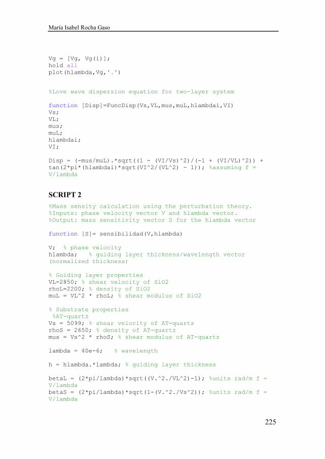
María Isabel Rocha Gaso
225
Vg = [Vg, Vg(i)];
hold all
plot(hlambda,Vg,'.')
%Love wave dispersion equation for two-layer system
function [Disp]=FuncDisp(Vs,VL,mus,muL,hlambdai,VI)
Vs;
VL;
mus;
muL;
hlambdai;
VI;
Disp = (-mus/muL).*sqrt((1 - (VI/Vs)^2)/(-1 + (VI/VL)^2)) +
tan(2*pi*(hlambdai)*sqrt(VI^2/(VL^2) - 1)); %assuming f =
V/lambda
SCRIPT 2
%Mass sensity calculation using the perturbation theory.
%Inputs: phase velocity vector V and hlambda vector.
%Output: mass sensitivity vector S for the hlambda vector
function [S]= sensibilidad(V,hlambda)
V; % phase velocity
hlambda; % guiding layer thickness/wavelength vector
(normalized thickness)
% Guiding layer properties
VL=2850; % shear velocity of SiO2
rhoL=2200; % density of SiO2
muL = VL^2 * rhoL; % shear modulus of SiO2
% Substrate properties
%AT-quartz
Vs = 5099; % shear velocity of AT-quartz
rhoS = 2650; % density of AT-quartz
mus = Vs^2 * rhoS; % shear modulus of AT-quartz
lambda = 40e-6; % wavelength
h = hlambda.*lambda; % guiding layer thickness
betaL = (2*pi/lambda)*sqrt((V.^2./VL^2)-1); %units rad/m f =
V/lambda
betaS = (2*pi/lambda)*sqrt(1-(V.^2./Vs^2)); %units rad/m f =
V/lambda
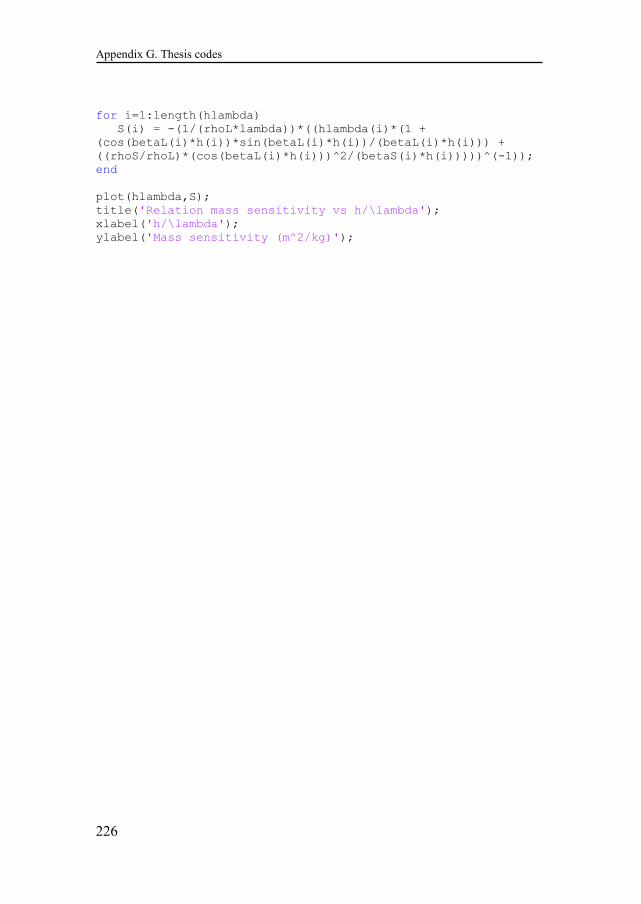
Appendix G. Thesis codes
226
for i=1:length(hlambda)
S(i) = -(1/(rhoL*lambda))*((hlambda(i)*(1 +
(cos(betaL(i)*h(i))*sin(betaL(i)*h(i))/(betaL(i)*h(i))) +
((rhoS/rhoL)*(cos(betaL(i)*h(i)))^2/(betaS(i)*h(i)))))^(-1));
end
plot(hlambda,S);
title('Relation mass sensitivity vs h/\lambda');
xlabel('h/\lambda');
ylabel('Mass sensitivity (m^2/kg)');
María Isabel Rocha Gaso
227
List of scientific communications
Peer-reviewed publications:
• M.-I. Rocha-Gaso, C. March-Iborra, A. Montoya-Baides, and A. Arnau-Vives, Surface generated acoustic wave biosensors for the detection of pathogens: a review, Sens. (Basel), 9 (2009) p. 5740-5769.
Book chapters:
• M.-I. Rocha-Gaso, Y. Jiménez, L.A. Francis, and A. Arnau-Vives, Love Wave Biosensors: a Review, InTech, p. 277-310, 2013.
Proceedings in international congresses:
• M.-I. Rocha-Gaso, R. Fernandez-Díaz, C. March-Iborra, and A. Arnau-Vives, Mass sensitivity evaluation of a Love wave sensor using the 3D Finite Element Method, IEEE Int. Freq. Control Symp, New Beach, USA, 2010.
Proceedings in national congresses:
• M.-I. Rocha-Gaso, R. Fernandez-Díaz, C. March-Iborra, Y.-J. Montagut-Ferizzola, and A. Arnau-Vives, Análisis de la sensibilidad de masa de un sensor Love mediante la simulación tridimensional con elementos finitos para aplicaciones en biosensores, Procc. Congreso Anual de la Sociedad Española de Ingeniería Biomédica (CASEIB), 2009, p. 205.
• Y.-J. Montagut-Ferizzola, J.-V. García-Narbón, M.-I. Rocha-Gaso, A. Arnau-Vives, Interfaz para la microbalanza de cuarzo (QCM) basada en osciladores que permite la aplicación de biosensores.
Appendix G. Thesis codes
228
Procc. Congreso Anual de la Sociedad Española de Ingeniería Biomédica (CASEIB), 2009, p. 235.
Oral presentations in international congresses:
• M.-I. Rocha-Gaso, J.V. García, C. March, Y. Jiménez, A. Montoya, and A. Arnau, Love Wave SAW Immunosensor for Detection of Carbaryl Pesticide, 3rd International Conference on Bio-Sensing Technology, Sitges, Spain, May 2013.
Posters in international congresses:
• M.-I. Rocha-Gaso, R. Fernandez-Díaz, C. March-Iborra, and A. Arnau-Vives, Mass sensitivity evaluation of a Love wave sensor using the 3D Finite Element Method, IEEE Int. Freq. Control Symp., New Beach, USA, 2010.
• M.I. Rocha-Gaso, C. March, J. García, L. El Fissi, L.A. Francis, Y. Jiménez, A. Montoya, and A. Arnau, User-friendly love wave flow cell for biosensors, Biosensors 2012, Cancun, Mexico., 2012.
Seminars:
• M.I. Rocha-Gaso, “Acoustic Wave Sensors”, Université catholique de Lovain, Lovain-la-Neuve, Belgium, February 25th, 2010.
• M.I. Rocha-Gaso, “Sensores de Onda Acústica de Superficie”, Universidad Politécnica de Valencia, Valencia, Spain, May 10th, 2010.
• M.I. Rocha-Gaso, “Acoustic Wave Sensors”, Universidad Politécnica de Valencia, Valencia, Spain, December 18th, 2012.
• M.I. Rocha-Gaso, “Acoustic Wave Sensors”, Universidad Politécnica de Valencia, Valencia, Spain, May 10th, 2013.
• M.I. Rocha-Gaso, “Analysis, implementation and validation of a Love mode surface acoustic wave device for its application as sensor of biological processes in liquid media”, Université catholique de Lovain, Lovain-la-Neuve, Belgium, June 18th, 2013.
María Isabel Rocha Gaso
229
References
[1] F. Kardous, L. El Fissi, J.-M. Friedt, F. Bastien, W. Boireau, R. Yahiaoui, J.F. Manceau, and S. Ballandras, Integrated active mixing and biosensing using low frequency vibration mixer and Love-wave sensor for real time detection of antibody binding event, J. Appl. Phys., 109 (2011) 1-8.
[2] P. Leonard, S. Hearty, J. Brennan, L. Dunne, J. Quinn, T. Chakraborty, and R. O'Kennedy, Advances in biosensors for detection of pathogens in food and water, Enzyme Microb. Technol., 32 (2003) 3-13.
[3] D. Ivnitski, I. Abdel-Hamid, P. Atanasov, and E. Wilkins, Biosensors for the detection of pathogenic bacteria, Biosens.
Bioelectron., 14 (1999) 599-624. [4] Anon., Waterborne pathogens kill 10M-20M people/year. World
Water Environment . 1996. [5] A.K. Deisingh and M. Thompson, Biosensors for the detection of
bacteria, Can. J. Microbiol., 50 (2004) 69-77. [6] March C., Manclús J.J., Abad A:, Navarro A., and Montoya A.,
Rapid detection and counting of viable beer-spoilage lactic acid bacteria using monoclonal chemiluminiscente enzyme immunoassay and CCD camera, J. Immunol. Methods, 303 (2005) 92-104.
[7] T. Pogfai, W. Krongkamol, S. Mongpraneet, A. Wisitsoraat, and A. Tuantranont, Low cost and portable PCR thermoelectric cycle, Int.
J. Appl. Biomed. Eng., 1 (2008) 41-45. [8] Abad, A., Producción de anticuerpos monoclonales y desarrollo de
inmunoensayos para el plaguicida carbaryl, PhD, Universitat Politècnica de València, 1996.
[9] C. March, J.J. Manclús, Y. Jiménez, A. Arnau, and A. Montoya, A piezoelectric immunosensor for the determination of pesticide residues and metabolites in fruit juices, Talanta, 78 (2009) 827-833.
[10] M.-I. Rocha-Gaso, C. March-Iborra, A. Montoya-Baides, and A. Arnau-Vives, Surface generated acoustic wave biosensors for the detection of pathogens: a review, Sens. (Basel), 9 (2009) 5740-5769.
References
230
[11] Francis, L. A., Thin film acoustic waveguides and resonators for gravimetric sensing applications in liquid, PhD Thesis, Université catholique de Louvain, 2006.
[12] E. Mauriz, A. Calle, A. Abad, A. Montoya, A. Hildebrandt, D. Barcelo, and L.M. Lechuga, Determination of carbaryl in natural water samples by a surface plasmon resonance flow-through immunosensor, Biosens. Bioelectron., 21 (2006) 2129-2136.
[13] A. Abad, J. Primo, and A. Montoya, Development of an enzyme-linked immunosorbent assay to carbaryl. 1. Antibody production form several haptens and characterization in different immunoassay formats, J. Agr. Food Chem., 45 (1997) 1486-1494.
[14] S. Varfolomeyev, I. Kurochkin, A. Eremenko, and E. Efremenko, Chemical and biological safety. Biosensors and nanothechnological methods for the detection and monitoring of chemical and biologica agents, Pure Appl. Chem., 74 (2002) 2311-2316.
[15] P. D'Orazio, Biosensors in clinical chemistry - 2011 update, Clin.
Chim. Acta, 412 (2003) 1749-1761. [16] Montoya A., Ocampo A., and March C., Fundamentals of
piezoelectric immunosensors, in: Arnau A. (Ed.), Piezoelectric transducers and applications, Springer, Berlin Heidelberg, 2008, pp. 289-306.
[17] S.Y. Yurish, N.V. Kirianaki, and I.L. Myshkin, World sensors and MEMS markets: analysis and trends, Sens. Transducers Mag., 62 (2005) 456-561.
[18] R.M. Lec and P.A. Lewin, Acoustic wave biosensors, Proc. 20th Annual Int. Conf. IEEE Eng. Med. Biol. Soc., 1998, pp. 2779-2784.
[19] Y. Montagut, J.V. García, Y. Jiménez, C. March, A. Montoya, and A. Arnau, QCM technology in biosensors, in: P. Andrea-Serra (Ed.), Biosensors- Emerging Materials and Applications, InTech, 2011, pp. 153-178.
[20] T. Wink, J.V. Zuilen, A. Bult, and P.V. Bennekom, Self-assembled monolayers for biosensors, Analyst, 122 (1997) 43-50.
[21] S.S. Iqbal, M.W. Mayo, J.G. Bruno, B.V. Bronk, C.A. Batt, and J.P. Chambers, A review of molecular recognition technologies for detection of biological threat agents, Biosens. Bioelectron., 15 (2000) 549-578.
[22] E. Hawkins, M. Cooper, and I. Campbell, Acoustic detection technology in the analysis of biomolecular interactions, Innov.
Pharm. Technol., 21 (2006) 30-34. [23] J.L. Marty, B. Leca, and T. Noguer, Biosensors for the detection of
pesticides, Analusis, 26 (1998) 144-149.
María Isabel Rocha Gaso
231
[24] M.P. Byfield and R.A. Abuknesha, Biochemical aspects of biosensors, Biosens. Bioelectron., 9 (1994) 373-400.
[25] A. Janshoff, H.J. Galla, and C. Steinem, Piezoelectric mass-sensing devices as biosensors- an alternative to optical biosensors?, Angew.
Chem. Int. Ed., 39 (2000) 4005-4032. [26] Y.S. Fung and Y.Y. Wong, Self-assembled monolayers as the
coating in a quartz piezoelectric crystal immunosensor to detect Salmonella in aqueous solution, Anal. Chem., 73 (2001) 5302-5309.
[27] X. Su, S.F.Y. Li, W. Liu, and J. Kwang, Piezoelectric quartz crystal based screening test for porcine reproductive and respiratory syndrome virus infection in pigs, Analyst, 125 (2000) 725-730.
[28] E. Gizeli and C.R. Lowe, Biomolecular sensors, Taylor & Francis, 2002.
[29] K.V. Singh, J. Kaur, G.C. Varshney, M. Raje, and C.R. Suri, Synthesis and characterization of hapten-protein conjugates for antibody production against small molecules, Bioconjug. Chem., 15 (2004) 168-173.
[30] M. Franek and K. Hruska, Antibody based methods for environmental and food analysis: a review, Vet. Med. -Czech, 50 (2005) 1-10.
[31] J.J. Manclus, A. Abad, M.Y. Lebedev, F. Mojarrad, B. Mickova, J.V. Mercader, J. Primo, M.A. Miranda, and A. Montoya, Development of a monoclonal immunoassay selective for chlorinated cyclodiene insecticides, J. Agric. Food Chem., 52 (2004) 2776-2784.
[32] K. Bizet, C. Gabrielli, H. Perrot, and J. Therasse, Validation of antibody-based recognition by piezoelectric transducers through electroacoustic admittance analysis, Biosens. Bioelectron., 13 (1998) 259-269.
[33] S. Tombelli and M. Mascinis, Piezoelectric quartz crystal biosensors: recent immobilization schemes, Anal. Lett., 33 (2000) 2129-2151.
[34] J. Pribyl, M. Hepel, J. Halámek, and P. Skládal, Development of piezoelectric immunosensors for competitive and direct determination of atrazine, Sens. Actuators B, 91 (2003) 333-341.
[35] Ch. Duan and M.E. Meyerhoff, Immobilization of proteins on gold coated porous membranes via ativated self-assembled monolayer of thioctic acid, Mikrochim. Acta, 117 (1995) 195-206.
[36] D.M. Disley, D.C. Cullen, H.-X. You, and C.R. Lowe, Covalent coupling of immunoglobulin G to self-assembled monolayers as method for immobilizing the interfacial-recongnition layer of a
References
232
surface plasmon resonance immunosensor, Biosens. Bioelectron., 13 (1998) 1213-1225.
[37] M. Prohanka and P. Skládal, Piezoelectric immunosensor for francisella tularensis detection using immunoglobulin m in a limiting dilution, Anal. Lett., 38 (2005) 411-422.
[38] S. Ferreti, S. Paynter, D.A. Russell, and K.E. Sapsford, Self-assembled monolayers: a versatile tool for the formulation of bio-surfaces, Trends Anal. Chem., 19 (2000) 530-540.
[39] R.D. Vaughan, C.K. O'Sullivan, and G.G. Guilbault, Sulfur based self-assembled monolayers (SAM´s) on piezoelectric crystals for immunosensor development, Fresentius J. Anal. Chem., 364 (1999) 54-57.
[40] E. Mauriz, E. Calle, L.M. Lechuga, J. Quintana, A. Montoya, and J.J. Manclús, Real-time detection of chlorpyrifos at part per trillion levels in ground, surface and drinking water samples by a portable Surface Plasmon Resonance immunsensor, Anal. Chim. Acta., 561 (2006) 40-47.
[41] E. Briand, M. Salmain, J.M. Herry, H. Perrot, C. Compere, and C.M. Pradier, Building of an immunosensor: how can the composition and structure of the thiol attachment layer affect the immunosensor efficiency?, Biosens. Bioelectron., 22 (2006) 440-448.
[42] S. Susmel, G.G. Guilbault, and C.K. O'Sullivan, Demonstration of labeless detection of food pathogens using electrochemical redox probe and screen printed gold electrodes, Biosens. Bioelectron., 18 (2003) 881-889.
[43] G.L. Coté, R.M. Lec, and M.V. Pishko, Emerging biomedical sensing technologies and their applications, IEEE Sens. J., 3 (2003) 251-266.
[44] A. Campitelli and E. Parton, MEMS-BioMEMS: Marrying ICs and biotech, Solid State Technol., 45 (2002) 87.
[45] W. Sant, M. Pourciel, J. Launay, T.D. Conto, A. Martinez, and P. Temple-Boyer, Development of chemical field effect transistors for the detection of urea, Sens. Actuators B, 95 (2003) 309.
[46] D.J. Webb, Optical-Fiber Sensors: An Overview, MRS Bulletin, (2002) 359-364.
[47] Gawad, S. D., PhD Thesis, Ecole Polytechnique Fédérale de Lausanne (EPFL), 2004.
[48] C. Koblinger, E. Uttenthaler, S. Drost, F. Aberl, H. Wolf, G. Brink, A. Stanglmaier, and E. Sackmann, Comparison of the QCM and the SPR method for surface studies and immunological applications, Sens. Actuators B, 24 (1995) 107.
María Isabel Rocha Gaso
233
[49] T.M. Chinowsky, J.G. Qionn, D.U. Bartholomew, R. Kaiser, and J.L. Elkind, Performance of the Spreeta 2000 integrated surface plasmon resonance affinity sensor, Sens. Actuators B, 91 (2003) 266-274.
[50] R.M. Lec, Piezoelectric biosensors, Proc. IEEE Int. Freq. Cont.
Symp., (2001). [51] G. Sauerbrey, The use of quartz oscillators for weighing thin layers
and for microweighing, Zeitschrift für Physik. C, Particles and fields, 1959, pp. 155-206.
[52] A.A. Oliner, Microwave network methods for guided elastic waves, IEEE Trans. Microwave Theory Tech., 17 (1969) 812-826.
[53] L.A. Francis, J.M. Friedt, C. Zhou, and P. Bertrand, In situ evaluation of density, viscosity, and thickness of adsorbed soft layers by combined surface acoustic wave and surface plasmon resonance, Anal. Chem., 78 (2006) 4200-4209.
[54] J. Rickert, W. Göpel, G.L. Hayward, B.A. Cavic, and M. Thompson, Biosensors based on acoustic wave devices, Sens.
Update, 5 (2001) 105-139. [55] J.W. Grate and G.C. Frye, Acoustic wave sensors, in: W. Göpel and
J. Hesse (Eds.), Sens. Update, Vol. 2. Wiley-VCH, Weinheim, 1996.
[56] T. Kogai and H. Yatsuda, Liquid sensor using SAW and SH-SAW on quartz, Proc. IEEE Ultrason. Symp., (2006) 552-555.
[57] J.C. Andle and J.F. Vetelino, Acoustic wave biosensors, Sens.
Actuators A, 44 (1994) 167-176. [58] J.P. Smith and V. Hinson-Smith, Commercial SAW sensors move
beyond military and security applications, Anal. Chem., (2006) 3505-3507.
[59] J.W. Grate, J.M. Stephen, and M.W. Richard, Acoustic wave microsensors, Anal. Chem., 65 (1993) 940A-848A.
[60] K. Länge, B.E. Rapp, and M. Rapp, Surface acoustic wave biosensors: a review, Anal. Bioanal. Chem., 391 (2008) 1509-1519.
[61] T.M. Gronewold, Surface acoustic wave sensors in the bioanalytical field: recent trends and challenges, Anal. Chim. Acta, 603 (2007) 119-128.
[62] K.K. Kanazawa and J.G. Gordon, Frequency of a quartz microbalance in contact with liquid, Anal. Chem., 57 (1985) 1770-1771.
[63] K.M. Lakin, G.R. Kline, and K.T. McCarron, High Q microwave acoustic resonators and filters, IEEE Trans. Microw. Theory Tech., 41 (1993) 2139-2146.
References
234
[64] J. Weber, M. Link, R. Primig, D. Pitzer, W. Wersing, and M. Schreiter, Investigation of the scaling rules determining the performance of film bulk acoustic resonators operating as mass sensors, IEEE Trans. Ultrason. Ferroelectr. Freq. Cont., 54 (2007) 405-412.
[65] L.M. Furtado, H. Su, M. Thompson, D.P. Mack, and G.L. Hayward, Interactions of HIV-1 TAR RNA with Tat-derived peptides discriminated by on-line acoustic wave detector, Anal. Chem., 71 (1999) 1167-1175.
[66] I. Ben-Dov, I. Willner, and E. Zisman, Piezoelectric immunosensors for urine specimens of Chlamydia trachomatis employing quartz crystal microbalance microgravimetric analyses, Anal. Chem., 69 (1997) 3506-3512.
[67] F. Hook, A. Ray, B. Norden, and B. Kasemo, Characterization of PNA and DNA immobilization and subsequent hybridization with DNA using acoustic-shear-wave attenuation measurements, Langmuir, 17 (2001) 8305-8312.
[68] A. Hengerer, C. Kosslinger, J. Decker, S. Hauck, I. Queitsch, H. Wolf, and S. Dubel, Determination of phage antibody affinities to antigen by a microbalance sensor system, Biotechniques, 26 (1999) 956-60, 962, 964.
[69] X. Zhou, L. Liu, M. Hu, L. Wang, and J. Hu, Detection of hepatitis B virus by piezoelectric biosensor, J. Pharm. Biomed. Anal., 27 (2002) 341-345.
[70] Y.S. Fung and Y.Y. Wong, Self-assembled monolayers as the coating in a quartz piezoelectric crystal immunosensor to detect Salmonella in aqueous solution, Anal. Chem., 73 (2001) 5302-5309.
[71] L. Richert, P. Lavalle, D. Vautier, B. Senger, J.F. Stoltz, P. Schaaf, J.C. Voegel, and C. Picart, Cell interactions with polyelectrolyte multilayer films, Biomacromolecules., 3 (2002) 1170-1178.
[72] M. Stobiecka, M. Jaroslaw, B. Janowska, B. Tudek, and H. Radecka, Piezoelectric sensor for determination of genetically modified soybean roundup readyâ in samples not amplified by PCR, Sens., 7 (2007) 1462-1479.
[73] Z. Lin, C.M. Yip, I.S. Joseph, and M.D. Ward, Operation of an ultrasensitive 30-MHz quartz crystal microbalance in liquids, Anal.
Chem., 65 (1993) 1546. [74] G. McHale, M.I. Newton, and F. Martin, Theoretical mass, liquid,
and polymer sensitivity of acoustic wave sensors with viscoelastic guiding layers, Appl. Phys. Lett., 93 (2003) 675-690.
María Isabel Rocha Gaso
235
[75] T. Tatsuma, Y. Watanabe, N. Oyama, K. Kitakizaki, and M. Haba, Multichannel quartz crystal microbalance, Anal. Chem., 71 (1999) 3632-3636.
[76] Mathias, L., Study and realization of shear wave mode solidly mounted film bulk acoustic resonators (FBAR) made of c-axis inclined zinc oxide (ZnO) thin films: application as gravimetric sensor in liquid environments, PhD Thesis, Université Henri Poincaré, 2006.
[77] C. Vale, J. Rosenbaum, S. Horwitz, S. Krishnaswamy, and R. Moore, FBAR filters at GHz frequencies, Proc. IEEE Ultrason.
Symp., (1990) 332-336. [78] R. Galb, M. Schreiter, E. Green, H.D. Feucht, H. Zeininger, J.
Runck, W. Reichl, R. Primig, D. Pitzer, G. Eckstein, and W. Wersing, Novel integrated FBAR sensors: a universal technology platform for bio-and gas-detection, Proc. IEEE Sens., (2011) 1184.
[79] R. Gabl, H.D. Feucht, H. Zeininger, G. Eckstein, M. Schreiter, R. Primig, D. Pitzer, and W. Wersing, First results on label-free detection of DNA and protein molecules using a novel integrated sensor technology based on gravimetric detection principles, Biosens. Bioelectron., 19 (2004) 615-620.
[80] J. Bjurstrom, G. Wingqvist, and I. Katardjiev, Synthesis of textured thin piezoelectric AlN films with a nonzero c-axis mean tilt for the fabrication of shear mode resonators, IEEE Trans. Ultrason.
Ferroelectr. Freq. Cont., 53 (2006) 2095-2100. [81] J. Weber, W.M. Albers, J. Tuppurainen, M. Link, R. Gabl, W.
Wersing, and M. Schreiter, Shear mode FBARs as highly sensitive liquid biosensors, Sens. Actuators A, 128 (2006) 84-88.
[82] G. Wingqvist, J. Bjurstrom, L. Liljeholm, V. Yantchev, and I. Katardjiev, Shear mode AlN thin film electro-acoustic resonant sensor operation in viscous media, Sens. Actuators B, 123 (2007) 466-473.
[83] G. Wingqvist, V. Yantchev, and I. Katardjiev, Mass sensitivity of multilayer thin film resonant BAW sensors, Sens. Actuators A, 148 (2008) 88-95.
[84] G. Wingqvist, H. Anderson, C. Lennartsson, T. Weissbach, V. Yantchev, and A.L. Spetz, On the applicability of high frequency acoustic shear mode biosensing in view of thickness limitations set by the film resonance, Biosens. Bioelectron., 24 (2009) 3387-3390.
[85] Francis, L. A., SAW sensors, Bachelor's Thesis, Université caholique de Louvain, 2000.
[86] R.M. White and F.W. Voltmer, Direct piezoelectric coupling to surface elastic waves, Appl. Phys. Lett., 7 (1965) 314-316.
References
236
[87] A. Arnau, Piezoelectric transducers and applications, Springer, Berlin Heidelberg, 2008.
[88] E. Berkenpas, S. Bitla, and C.M. Pereira da, LGS shear horizontal SAW devices for biosensor applications, Proc. IEEE Ultrason. Symp., 2003, pp. 1404-1407.
[89] R.L. Baer and C.A. Flory, Some limitations on the use of leaky SAW mode sensors in liquids, Proc. IEEE Ultrason. Symp., Orlando, USA., 1991, pp. 279-284.
[90] T. Wessa, N. Barié, M. Rapp, and H.J. Ache, Polyimide, a new shielding layer for sensor applications, Sens. Actuators B, 53 (1998) 63-68.
[91] N. Barié, M. Rapp, H. Sigrist, and H.J. Ache, Covalent photolinker-mediated immobilization of an intermediate dextran layer to polymer-coated surfaces for biosensing, Biosens.
Bioelectron., 13 (1998) 855-860. [92] D.D. Deobagkar, V. Limaye, S. Shinha, and R.D.S. Yadava,
Acoustic wave immunosensing of Excherichia coli in water, Sens.
Actuators B, 104 (2005) 85-89. [93] J.E. Roederer and G.J. Bastiaans, Microgravimetric immunoassay
with piezoelectric crystals, Anal. Chem., 55 (1983) 2333-2336. [94] J. Hechner and W. Soluch, Pseudo surface acoustic wave dual
delay line on 41° YX LiNbO3 for liquid sensors, Sens. Actuators B, 111-112 (2005) 436-440.
[95] X. Lu, Y. Luo, P. Wang, and M. Deng, The small volume liquid density sensor using surface acoustic wave, Proc. IEEE Int. Conf. Mechantron. Autom., 2006, pp. 2105-2110.
[96] V.S. Chivukula, M.S. Shur, and D. Ciplys, Recent advances in application of acoustic, acousto-optic and photoacoustic methods in biology and medicine, Physica status solidi, 204 (2007) 3209-3236.
[97] K. Yamanouchi and K. Shibayama, Propagation and amplification of Rayleigh waves and piezoelectric leaky surface waves in LiNbO, J. Appl. Phys., 43 (1972) 856-862.
[98] K. Nakamura, Piezoelectric applications of ferroelectric single crystals, Proc. 13th IEEE Int. Symp. Appl. Ferroelectr., 2002, pp. 389-394.
[99] T.B. Pollard, T.D. Kenny, J.F. Vetelino, and M. Pereira da Cunha, Pure SH-SAW propagation, transduction measurements on KNbO3, IEEE Trans. Ultrason. Ferroelectr. Freq. Cont., 53 (2006) 199-208.
[100] E. Berkenpas, P. Millard, and C.M. Pereira da, Detection of Escherichia coli O157:H7 with langasite pure shear horizontal surface acoustic wave sensors, Biosens. Bioelectron., 21 (2006) 2255-2262.
María Isabel Rocha Gaso
237
[101] S. Rupp, M. Von Schickfus, S. Hunklinger, H. Eipel, A. Priebe, D. Enders, and A. Pucci, A shear horizontal surface acoustic wave sensor for the detection of antigen-antibody reactions for medical diagnosis, Sens. Actuators B, 134 (2008) 225-229.
[102] S. Shiokawa and T. Moriizumi, Design of SAW sensor in liquid : SAW and communication devices, Japanese J. of Appl. Phys., 27 (1988) 142-144.
[103] M. Rapp, H. Wessa, and H.J. Ache, Modification of commercially availabel low-loss SAW devices towards an immunosensor for in-situ measurements in water, Proc. IEEE Ultrason. Symp., Seattle, USA., 1995, pp. 433-436.
[104] R.E. Milsom, N.H.C. Reilly, and M. Redwood, Analysis of generation and detection of surface an bulk acoustic waves by interdigital transducers, IEEE Trans. Sonics Ultrason., SU-24 (1997) 147-166.
[105] M. Lewis, Surface skimming bulk waves, SSBW, Proc. IEEE Ultrason. Symp., 1977, pp. 744-752.
[106] T.L. Bagwell and R.C. Bray, Novel surface transverse wave resonators with low loss and high Q, Proc. IEEE Ultrason. Symp., 1987, pp. 319-323.
[107] M. Tom-Moy, R.L. Baer, D. Spira-Solomon, and T.P. Doherty, Antrizine measurements using surface transverse wave devices, Anal. Chem., 67 (1995) 1510-1516.
[108] R.L. Baer, C.A. Flory, M. Tom-Moy, and D.S. Solomon, STW chemical sensors, Proc. IEEE Ultrason. Symp., Tucson, USA., 1992, pp. 293-298.
[109] V. Ferrari and R. Lucklum, Overview of Acoustic-Wave Microsensors, in: A. Arnau (Ed.), Piezoelectric transducers and applications, Springer, Berlin Heidelberg, 2008, pp. 39-59.
[110] V.L. Strashilov and V.M. Yantchev, Surface transverse waves: properties, devices, and analysis, IEEE Trans. Ultrason.
Ferroelectr. Freq. Cont., 52 (2005) 812-821. [111] A.E.H. Love, Some problems of geodynamics, Cambridge
University Press, 1911. [112] M.V. Voinova, On Mass Loading and Dissipation Measured with
Acoustic Wave Sensors: A Review, J. Sens., (2009) 1-13. [113] J. Du, G.L. Harding, J.A. Ogilvy, P.R. Dencher, and M. Lake, A
study of Love-wave acoustic sensors, Sens. Actuators A, 56 (1996) 211-219.
[114] K. Kalantar-Zadeh, W. Wlodarski, Y.Y. Chen, B.N. Fry, and K. Galatsis, Novel Love mode surface acoustic wave based immunosensors, Sens. Actuators B, 91 (2003) 143-147.
References
238
[115] J. Du and G.L. Harding, A multilayer structure for Love-mode acoustic sensors, Sens. Actuators A, 65 (1998) 152-159.
[116] E. Gizeli, N.J. Goddard, C.R. Lowe, and A.C. Stevenson, A Love plate biosensor utilising a polymer layer, Sens. Actuators B, 6 (1992) 131-137.
[117] F. Herrmann, M. Weihnacht, and S. Buttgenbach, Properties of sensors based on shear-horizontal surface acoustic waves in LiTaO3/SiO2 and quartz/SiO2 structures, IEEE Trans. Ultrason.
Ferroelectr. Freq. Cont., 48 (2001) 268-273. [118] K. Kalantar-Zadeh, D.A. Powell, A.Z. Sadek, W. Wlodarski, Q.B.
Yang, and Y.X. Li, Comparison of ZnO/64° LiNbO3 and ZnO/36° LiTaO3 surface acoustic wave devices for sensing applications, Sens. Lett., 4 (2006) 135-138.
[119] F.S. Hickernell, H.D. Knuth, R.C. Dablemont, and T.S. Hickernell, The surface acoustic wave propagation characteristics of 64° YX LiNbO3 and 36° YX LiTaO3 substrates with thin-film SiO2, Proc. IEEE Ultrason. Symp., Seattle, USA., 1995, pp. 345-348.
[120] E. Gizeli, A.C. Stevenson, N.J. Goddard, and C.R. Lowe, A novel Love-plate acoustic sensor utilizing polymer overlayers, IEEE
Trans. Ultrason. Ferroelectr. Freq. Cont., 39 (1992) 657-659. [121] D.A. Powell, K. Kalantar-Zadeh, S. Ippolito, and W. Wlodarski,
3E- 2 A layered SAW device based on ZnO/LiTaO3 for liquid media sensing applications, Proc. IEEE Ultrason. Symp., 2002, pp. 493-496.
[122] K. Kalantar-Zadeh, A. Trinchi, W. Wlodarski, and A. Holland, A novel Love-mode device based on a ZnO/ST-cut quartz crystal structure for sensing applications, Sens. Actuators B, 100 (2009) 135-143.
[123] D.W. Branch and L.E. Thayne, 4D- 4 Love wave acoustic array biosensor platform for autonomous detection, Proc. IEEE Ultrason. Symp., 2007, pp. 260-263.
[124] D.S. Ballantine, R.M. White, S.J. Martin, A.J. Ricco, E.T. Zellers, G.C. Frye, and H. Wohltjen, Acoustic Wave Sensors: Theory, Design and Physico-Chemical Applications, Academic press, San Diego, 1997.
[125] C. Déjous, M. Savart, D. Rebière, and J. Pistré, A shear-horizontal acoustic plate mode (SH-APM) sensor for biological media, Sens.
Actuators B, 26-27 (1995) 452-456. [126] J.C. Andle, J.F. Vetelino, M.W. Lade, and D.J. McAllister, An
acoustic plate mode device for biosensing applications, Proc. Transducers 91 Int. Conf. Solid-State Sens. Actuators, San Francisco, USA., 1991, pp. 483-485.
María Isabel Rocha Gaso
239
[127] F. Bender, F. Meimeth, R. Dahing, M. Grunze, and F. Josse, Mechanisms of interaction in acostic plate mode immunosensors, Sens. Actuators B, 40 (1997) 105-110.
[128] G. McHale, M.I. Newton, and F. Martin, Theoretical mass sensitivity of Love wave and layer guided acoustic plate mode sensors, Appl. Phys. Lett., 91 (2002) 9701-9710.
[129] G. McHale, M.I. Newton, and F. Matin, Layer guided shear horizontally polarized acoustic plate modes, Appl. Phys. Lett., 91 (2002) 5735.
[130] C.R. Evans, S.M. Stanley, C.J. Percival, G. McHale, and M.I. Newton, Lithium tantalate layer guided plate mode sensors, Sens.
Actuators A, 132 (2006) 241-244. [131] Venema, A., Ph.D. Thesis Delft University of Technology, 1980. [132] R.M. White, P.J. Wicher, S.W. Wenzel, and E.T. Zellers, Plate-
mode ultrasonic oscillator sensors, IEEE Trans. Ultrason.
Ferroelectr. Freq. Cont., 34 (1987) 162-171. [133] S.W. Wenzel and R.M. White, A multisensor employing an
ultrasonic lamb-wave oscillator, IEEE Trans. Electron. Devices, 35 (1988) 735-743.
[134] M.J. Vellekoop, G.W. Lubking, P.M. Sarro, and A. Venema, Integrate-circuit-compatible design and technology of acoustic-wave-based microsensors, Sens. Actuators A, 44 (1994) 249-263.
[135] M. Nirschl, F. Reuter, and J. Voros, Review of transducer principles for label-free biomolecular interaction analysis, Biosensors, (2011) 70-92.
[136] G. Kovacs, G.W. Lubking, M.J. Vellekoop, and A. Venema, Love waves for (bio)chemical sensing in liquids, Proc. IEEE Ultrason. Symp., Tucson, USA., 1992, pp. 281-285.
[137] G.L. Harding, J. Du, P.R. Dencher, D. Barnett, and E. Howe, Love wave acoustic immunosensor operation in liquid, Sens. Actuators A, 61 (1997) 279-286.
[138] J. Freudenberg, S. Schelle, K. Beck, von Schickfus M., and Hunklinger S., A contactless surface acoustic wave biosensor, Biosens. Bioelectron., 14 (1999) 423-425.
[139] E. Howe and G. Harding, A comparison of protocols for the optimisation of detection of bacteria using a surface acoustic wave (SAW) biosensor, Biosens. Bioelectron., 15 (2000) 641-649.
[140] O. Tamarin, S. Comeau, C. Déjous, D. Moynet, D. Rebière, J. Bezian, and J. Pistré, Real time device for biosensing: design of a bacteriophage model using love acoustic wave, Biosens.
Bioelectron., 18 (2003) 755-763.
References
240
[141] M.D. Schlensog, M.A. Thomas, T.M. Gronewold, M. Tewes, M. Famulok, and E. Quandt, A Love-wave biosensor using nucleic acids as ligands, Sens. Actuators B, 101 (2004) 308-315.
[142] D.W. Branch and S.M. Brozik, Low-level detection of a Bacillus anthracis simulant using Love-wave biosensors on 36° YX LiTaO3, Biosens. Bioelectron., 19 (2004) 849-859.
[143] N. Moll, E. Pascal, D.H. Dinh, J.P. Pillot, B. Bennetau, D. Rebiere, D. Moynet, Y. Mas, D. Mossalayi, J. Pistre, and C. Dejous, A Love wave immunosensor for whole E. coli bacteria detection using an innovative two-step immobilisation approach, Biosens. Bioelectron., 22 (2007) 2145-2150.
[144] N. Moll, E. Pascal, D.H. Dinh, J.-L. Lachaud, L. Vellutini, J.-P. Pillot, D. Rebière, D. Moynet, J. Pistré, D. Mossalayi, Y. Mas, B. Bennetau, and C. Déjous, Multipurpose Love acoustic wave immunosensor for bacteria, virus or proteins detection, ITBM-RBM, 29 (2008) 155-161.
[145] J. Andrä, A. Böhling, T.M.A. Gronewold, U. Schlecht, M. Perpeet, and T. Gutsmann, Surface acoustic wave biosensor as a tool to study the interactions of antimicrobial peptides with phospholipid and lipopolysaccharide model membranes, Langmuir, 24 (2008) 9148-9153.
[146] M. Bisoffi, B. Hjelle, D.C. Brown, D.W. Branch, T.L. Edwards, S.M. Brozik, V.S. Bondu-Hawkins, and R.S. Larson, Detection of viral bioagents using a shear horizontal surface acoustic wave biosensor, Biosens. Bioelectron., 23 (2008) 1397-1403.
[147] L. El Fissi, J.-M. Friedt, V. Luzet, F. Chérioux, G. Martin, and S. Ballandras, A Love-wave sensor for direct detection of biofunctionalized nanoparticles, IEEE, (2009) 861-865.
[148] O. Tigli, L. Binova, P. Berg, and M. Zaghloul, Fabrication and characterization of a Surface-Acoustic-Wave biosensor in CMOS Technology for cancer biomarker detection, IEEE Trans.
Biomedical. Circuit. Systems., 4 (2010) 62-73. [149] F. Fournel, E. Baco, M. Mamani-Matsuda, M. Degueil, B.
Bennetau, D. Moynet, D. Mossalayi, L. Vellutini, J.-P. Pillot, C. Dejous, and D. Rebiere, Love wave biosensor for real-time detection of okadaic acid as DSP phycotoxin, Proc. Eurosensors XXIV, Eurosensors XXIV, Linz, Austria, 2010, pp. 831-834.
[150] I. Gammoudi, H. Tarbague, J.L. Lachaud, S. Destor, A. Othmane, D. Moyenet, R. Kalfat, D. Rebiere, and C. Dejous, Love wave bacterial biosensors and microfluidic network for detection of heavy metal toxicity, Sens. Lett., 9 (2011) 816-819.
María Isabel Rocha Gaso
241
[151] H. Oh, Y. Lee, S. Lee, S.S. Yang, and K. Lee, Development of Novel LOVE wave biosensor for simultaneous detection of multi-analyte, Proc. Eurosensors XXV, Eurosensors XXV, Athens, Greece., 2011, pp. 908-911.
[152] T. Song, S.Y. Song, H.C. Yoon, and K. Lee, Development of a wireless Love wave biosensor platform for multi-functional detection, Japanese J. of Appl. Phys., 50 (2011) 1-6.
[153] D. Matatagui, M. Fernández, J. Fontecha, J. Santos, M. Horrillo, D. Moynet, J. Esquivel, C. Gracia, C. Cané, C. Dejous, and D. Rebière, Development of a Love-wave immunosensor with microfluidic technology to detect phages in dynamic mode, Proc. 14th International Meeting on Chemical Sensors, 14th Int. Meeting Chem. Sens., Nuremberg, Germany, 2012, pp. 892-895.
[154] M. Saitakis and E. Gizeli, Acoustic sensors as a biophysical tool for probing cell attachment and cell/surface interactions, Cell. Mol. Life
Sci., 69 (2012) 357-371. [155] K. Mitsakakis, S. Sekula-Neuner, S. Lenhert, H. Fuchs, and E.
Gizeli, Convergence of Dip-Pen Nanolithography and acoustic biosensors towards a rapid-analysis multi-sample microsystem, Analyst, 137 (2012) 3076.
[156] C.J. Cheng, C.T. Feng, K. Kalantar-Zadeh, and M.Z. Atashbar, Development of guided SH-SAW based wireless sensing platform for monitoring protein binding, Proc. 14th Int. Meeting Chem. Sens., 2012, pp. 1433-1436.
[157] K. Saha, F. Bender, A. Rasmusson, and E. Gizeli, Probing the viscoelasticity and mass of a surface-bound protein layer with an Acoustic Waveguide Device, Langmuir, 19 (2003) 1304-1311.
[158] A. Tsortos, G. Papadakis, K. Mitsakakis, K.A. Melzak, and E. Gizeli, Quantitative determination of size and shape of surface-bound DNA using an acoustic wave sensor, Biophys. J., 94 (2008) 2706-2715.
[159] G. Papadakis, A. Tsortos, and E. Gizeli, Triple-helix DNA structural studies using a Love wave acoustic biosensor, Biosens.
Bioelectron., 25 (2009) 702-707. [160] E. Gizeli, C.L. Lowe, M. Liley, and H. Vogel, Detection of
supported lipid layers with the acoustic Love waveguidedevice: application to biosensors, Sens. Actuators B, 34 (1996) 295-300.
[161] P. Bröker, K. Lücke, M. Perpeet, and T.M.A. Gronewold, A nanostructured SAW chip-based biosensor detection cancer cells, Sens. Actuators B, 165 (2012) 1-6.
[162] M. Marth, D. Maier, U. Stahl, M. Rapp, T. Wessa, and J. Honerkamp, Optimization of surface acoustic wave sensor arrays
References
242
and application to high performance liquid chromatography, Sens.
Actuators B, 61 (1999) 191-198. [163] A. Ballato, Piezoelectricity: old effect, new thrusts, IEEE Trans.
Ultrason. Ferroelectr. Freq. Cont., 42 (1995) 916-926. [164] D.A. Powell, K. Kalantar-Zadeh, W. Wlodarski, J. Samuel, and S.J.
Ippolito, Layered Surface Acoustic Wave Chemical and Bio-Sensors, Encycl. Sens., (2006) 1-18.
[165] Francis, L. A., Investigation of Love waves sensors. Optimisation for biosensing applications, Master Thesis, Université Catholique de Louvain, 2001.
[166] B. Jakoby, J. Bastemeijer, and M.J. Vellekoop, Temperature-compensated Love-wave sensors on quartz substrates, Sens.
Actuators A, 82 (2000) 83-88. [167] F. Herrmann and S. Büttgenbach, Temperature-compensated Shear
Horizontal surface acoustic wave in layered quartz/SiO2- structures, Physica status solidi, 170 (1998) R3-R4.
[168] O. Tamarin, C. Déjous, D. Rebiere, J. Pistré, S. Comeau, D. Moynet, and J. Bezian, Study of acoustic Love wave devices for real time bacteriophage detection, Sens. Actuators B, 91 (2003) 275-284.
[169] E. Gizeli, F. Bender, A. Rasmusson, K. Saha, F. Josse, and R. Cernosek, Sensitivity of the acoustic waveguide biosensor to protein binding as a funcion of the waveguide properties, Biosens.
Bioelectron., 18 (2003) 1399-1406. [170] D.A. Powell, K. Kalantar-Zadeh, and W. Wlodarski, Numerical
calculation of SAW sensitivity: application to ZnO/LiTaO3 transducers, Sens. Actuators A, 115 (2004) 456-461.
[171] M.S. Nieuwenhuizen and A. Venema, Surface acoustic wave chemical sensors, Sens. Mater., 5 (1989) 261-300.
[172] D.P. Morgan, Surface-Wave Devices for Signal Processing, Elsevier Science Publishers B.V., New York, 1991.
[173] El Fissi, L., Détection et mesure de nanoparticules pour les applications de capteurs en milieu liquide, PhD Thesis, Université de Franche-Comté, 2009.
[174] K.-Y. Hashimoto, Surface Acoustic Wave Devices in Telecommunications, Springer-Verlag, Berlin Heidelberg, 2000.
[175] C. Campbell, Surface acoustic wave devices and their signal processing applications, Academic Press, Sand Diego, 1989.
[176] Mazein, P., Étude de dispositifs à ondes de Love par modélisation numérique de la propagation d'ondes acoustiques. Application à l'optimisation de structures et à la caractérisation de matériaux en
María Isabel Rocha Gaso
243
vue de la réalisation de capteurs chimiques., PhD Thesis, L'Université Bordeaux I, 2005.
[177] N. Barié, T. Wessa, M. Bruns, and M. Rapp, Love waves in SiO2 layers on STW-resonators based on LiTaO3, Talanta, 62 (2004) 71-79.
[178] K. Kalantar-Zadeh, A. Trinchi, W. Wlodarski, and A. Holland, A novel Love-mode device based on a ZnO/ST-cut quartz crystal structure for sensing applications, Sens. Actuators A, 100 (2002) 135-143.
[179] D. Matatagui, J. Fontecha, M.J. Fernández, M. Aleixandre, I. Gracia, C. Cané, and M.C. Horrillo, Array of Love-wave sensors based on quartz/Novolac to detect CWA simulants, Talanta, 85 (2011) 1442-1447.
[180] F. Herrmann, D. Hahn, and S. Büttgenbach, Separate determination of liquid density and viscosity with sagitally corrugated Love mode sensors, Sens. Actuators A, 78 (1999) 99-107.
[181] S. Franssila, Introduction to Microbabrication, Wiley, 2004. [182] E. Gizeli, M. Liley, and C.L. Lowe, Design considerations for the
acoustic waveguide biosensor, Smart Mater. Struct., 6 (1997) 700-706.
[183] L. El Fissi, J.-M. Friedt, S. Ballandras, L. Robert, and F. Chérioux, Acoustic characterization of thin polymer layers for Love mode surface acoustic waveguide, Proc. IEEE Int. Freq. Control Symp., 2008, pp. 711-716.
[184] L.A. Francis, J.-M. Friedt, and P. Bertrand, Influence of electromagnetic interferences on the mass sensitiviy of Love mode surface acoustic wave sensors, Sens. Actuators A, 123-124 (2005) 360-369.
[185] B. Jakoby and M.J. Vellekoop, Viscous losses of shear waves in layered structures used for biosensing, Proc. IEEE Ultrason. Symp., 1998, pp. 493-496.
[186] B. Zimmermann, R. Lucklum, P. Hauptmann, J. Rabe, and S. Büttgenbach, Electrical characterisation of high-frequency thickness-shear-mode resonators by impedance analysis, Sens.
Actuators B, 76 (2001) 47-57. [187] Y. Montagut, J.V. García, Y. Jiménez, C. March, A. Montoya, and
A. Arnau, Validation of a phase-mass characterization concept and interface for acoustic biosensors, Sens. (Basel), 11 (2011) 4702-4720.
[188] Y.J. Montagut, J.V. García, Y. Jiménez, C. March, A. Montoya, and A. Arnau, Frequency-shift vs phase-shift characterization of in-
References
244
liquid quartz crystal microbalance applications, Rev. Sci. Instrum., 82 (2011) 064702.
[189] A. Abdollahi, A. Jiang, and S.A. Arabshahi, Evaluation on mass sensitivity of SAW sensors for different piezoelectric materials using finite-element analyisis, IEEE Trans. Ultrason. Ferroelectr.
Freq. Contr., 54 (2007) 2446-2455. [190] Z. Wang, J.D.N. Cheeke, and C.K. Jen, Sensitivity analysis for
Love mode acoustic gravimetric sensors, Appl. Phys. Lett., 64 (1994) 2940-2942.
[191] J. Liu and S. He, Theoretical analysis on Love waves in layered structure with a piezoelectric substrate and multiple elastic layers, J.
Appl. Phys., 107 (2010) 073511. [192] P. Kielczynski, M. Szalewski, and A. Balcerzak, Effect of a viscous
liquid loading on Love wave propagation, Int. J. Solids Struct., 49 (2012) 2314-2319.
[193] B.A. Auld, Acoustic fields and waves in solids, Krieger, Malabar, Florida, 1990.
[194] S.K.R.S. Sankaranarayanan, V.R. Bhethanabotla, and B. Joseph, Modeling of Surface Acoustic Wave Sensor Response, in: M.K. Ram and V.R. Bhethanabotla (Eds.), Sensors for Chemical and Biological Applications, CRC Press, 2010, pp. 97-134.
[195] V. Laude, A. Reinhardt, S. Ballandras, and A. Khelif, Fast FEM/BEM computation of SAW harmonic admittance and slowness curves, Proc. IEEE Ultrason. Symp., 2004, pp. 445-448.
[196] V.P. Plessky and T. Thorvaldsson, Rayleigh waves and leaky SAW's in periodic systems of electrodes: Periodic Green functions analysis, Electron. Lett., 28 (1992) 1317-1319.
[197] M.Z. Atashbar, B.J. Bazuin, M. Simpeh, and S. Krishnamurthy, 3D FE simulation of H2 SAW gas sensor, Sens. Actuators B, 111-112 (2005) 213-218.
[198] G. Xu, Finite element analysis of second order effects on the frequency response of a SAW device, Proc. Proc. IEEE Ultrason. Symp., Proc.IEEE Ultrason.Symp., 2000, pp. 187-190.
[199] S.J. Ippolito, K. Kalantar-Zadeh, D.A. Powell, and W. Wlodarski, A 3-dimensional finite element approach for simulating acoustic wave propagation in layered SAW devices, Proc. IEEE Ultrason. Symp., 2003, pp. 303-306.
[200] M.-I. Rocha-Gaso, R. Fernandez-Díaz, C. March-Iborra, and A. Arnau-Vives, Mass sensitivity evaluation of a Love wave sensor using the 3D Finite Element Method, Proc. IEEE Int. Freq. Control Symp., 2010.
María Isabel Rocha Gaso
245
[201] B. Jakoby and M.J. Vellekoop, Properties of Love waves: applications in sensors, Smart Mater. Struct., 6 (1997) 668-679.
[202] D. MacDougall, F.J. Amore, G.V. Cox, D.G. Crosby, F.L. Estes, and et.al, Guidelines for data acquisition and data quality evaluation in environmental chemistry, Anal. Chem., 52 (1980) 2242-2249.
[203] J. Du, D.R. Harding, A.F. Collings, and P.R. Dencher, An experimental study of Love-wave acoustic sensors operating in liquids, Sens. Actuators A, 60 (1997) 54-61.
[204] X. Chen, M. Anthamatten, and D.R. Harding, Vapor Deposition and Curing of Polybenzoxazole Precursors, Macromolecules, 39 (2006) 7561-7565.
[205] A. Turton, D. Bhattacharryya, and D. Wood, Liquid density analysis of sucrose andalcoholic beverages using polyimideguided Love-mode acoustic wave sensors, Meas. Sci. Technol., 17 (2006) 257-263.
[206] H.J. Lee, K. Namkoong, E.C. Cho, C. Ko, J.C. Park, and S.S. Lee, Surface acoustic wave immunosensor for real-time detection of hepatitis B surface antibodies in whole blood samples, Biosens.
Bioelectron., 24 (2009) 3120-3125. [207] G. Kovacs and A. Venema, Theoretical comparison of sensitivities
of acoustic shear wave modes for (bio) chemical sensing in liquids, Appl. Phys. Lett., 61 (1992) 639-641.
[208] B. Jakoby and M.J. Vellekoop, Viscosity sensing using a Love-wave device, Sens. Actuators A, 68 (1998) 275-281.
[209] S.D. Curtin, B. Jakoby, A. Berthold, V.K. Varadam, V.V. Varadam, and M.J. Vellekoop, A micromachined wet cell for a LW liquid sensor, Proc. SPIE Conf. Smart Electron. MEMS, 1998, p. 194.
[210] L.A. Francis, J.-M. Friedt, C. Bartic, and A. Campitelli, A SU-8 liquid cell for surface acoustic wave biosensors, Proc. SPIE Int. Soc. Opt. Eng., 2004, pp. 353-363.
[211] M.I. Rocha-Gaso, C. March, J. García, L. El Fissi, L.A. Francis, Y. Jiménez, A. Montoya, and A. Arnau, User-friendly love wave flow cell for biosensors, Biosensors 2012, Cancun, Mexico., 2012.
[212] H. Tarbague, L. Lachaud, L. Vellutini, J.P. Pillot, B. Bennetaur, D. Moynet, and D. Rebière, PDMS microfluidic chips combined to saw biosensors for ultra-fast biodetection of antibodies and E. coli bacteria, Biosensors 2012, Cancun, Mexico., 2012.
[213] Veeco, NanoScope Analysis program. Help Notes[1.10]. 2010. [214] Jiménez, Y., Contribución a la resolución de la problemática
asociada a la medida de las propiedades físicas de recubrimientos
References
246
viscoelásticos en sensores de cuarzo, Ph.D.Thesis, Universidad Politécnica de Valencia, 2004.
[215] S.J. Martin, V.E. Granstaff, and G.C. Frye, Characterizationof quartz crystal microbalance with simultaneous mass andliquid loading, Anal. Chem., 63 (1991) 2272-2281.
[216] A. Arnau, Y. Montagut, J.V. García, and Y. Jiménez, A different point of view on the sensitivity of quartz crystal microbalance sensors, Meas. Sci. Technol., 20 (2009) 124004.
[217] L. El Fissi, J.-M. Friedt, B. Belgacem, F. Chérioux, V. Luzet, and S. Ballandras, Fabrication and Packaging Technologies of Love-wave-based Microbalance for Fluid Analysis, Proc. Eurosensors XXIII conference, 2009, pp. 52-55.
[218] B.P. Sagmeister, I.M. Graz, R. Schwodiauer, H. Gruber, and S. Bauer, User-friendly, miniature biosensor flow cell for fragile high fundamental frequency quartz crystal resonators, Biosens.
Bioelectron., 24 (2009) 2643-2648. [219] J. García, C. March, A. Sánchez, Y. Montagut, A. Montoya, and A.
Arnau, High-sensitivity piezoelectric immunosensor for pesticide analysis, Biosensors 2012, Cancun, Mexico., 2012.
[220] Montagut, Y., Sistema oscilador mejorado para aplicaciones de microbalanza (QCM) en medios líquidos y propuesta de un nuevo método de caracterización para biosensores piezoeléctricos, PhD Thesis, Universidad Politécnica de Valencia, Spain, 2011.
[221] García-Narbón, J. V., Improved technique for the characterization of QCM resonators under high damping liquid media, and integrated platform for high frequency microbalace sensor monitoring in high resolution applications, PhD Thesis, Universidad Politécnica de Valencia, Spain. (in press), 2013.
[222] L.M. Sheely, Glycerol viscosity tables, Ind. Eng. Chem., 24 (1932) 1060-1064.
[223] A. Tsortos, G. Papadakis, and E. Gizeli, Molecular conformation biosensing. [WO 2008/155692]. 2008.
[224] Sanchez, A., Desarrollo y aplicación de inmunosensores para el análisis de contaminantes químicos en alimentos, Master Thesis, Universidad Politécnica de Valencia, 2011.
[225] M.P. Marco, S. Gee, and B.D. Hammock, Immunochemical techniques for environmental analysis II. Antobody production and immunoassay develpment, TrAC Trends in Analytical Chemistry, 14 (1995) 415-425.
[226] M.C. Estevez, J. Belenguer, S. Gomez-Montes, J. Miralles, A.M. Escuela, A. Montoya, and L.M. Lechuga, Indirect competitive immunoassay for the detection of fungicide Thiabendazole in whole
María Isabel Rocha Gaso
247
orange samples by Surface Plasmon Resonance, Analyst, 137 (2012) 5659-5665.
[227] A. Abad and A. Montoya, Development of an enzyme-linked immunosorbent assay to carbaryl. 2. Assay Optimization and Application to the Analysis of Water Samples, J. Agric. Food
Chem., 45 (1997) 1495-1501. [228] E.W. Weisstein, Lamé constants. 2007. 6-14-2010. [229] V. Kaajakari, Elastic constants silica. http://www.kaajakari.net .
2010. 7-7-2010. [230] H. Goldstein, C. Poole, and J. Safko, The kinematics of rigid body
motion, Classical Mechanics, Addison-Wesley, 2002, p. 134. [231] A.J. Slobodnik and E.D. Conway, Microwave Acoustics Handbook
Surface Wave Velocities, Bedford, MA: Air Force Cambridge Research Laboratories, 1973.
[232] W.G. Cady, Piezoelectricity. An Introduction to the Theory and Applications of Elechtromechanical Phenomena in Crystals, Dovers Publications, Inc., New York, 1964.
[233] IEEE Standard 176 on Piezoelectricity, IEEE, (1987). [234] W.G. Cady, Piezoelectricity. An introduction to the theory and
applications of elechtromechanical phenomena in crystals, Dovers Publications, Inc., New York, 1964.
[235] J.G. Gualtieri, J.A. Kosinski, and A. Ballato, Piezoelectric materials for acoustic wave applications, IEEE Trans. Ultrason.
Ferroelectr. Freq. Cont., 41 (1994) 53-59. [236] G. Kovacs, M. Anhom, H.E. Engan, G. Visintini, and C.C.W.
Ruppel, Improved Material Constants for LiNb03 and LiTaO3, Proc. IEEE Ultrason. Symp., 1990, pp. 435-438.
[237] J. Liu and S. He, Properties of Love waves in layered piezoelectric structures, Int. J. Solids Struct., 47 (2010) 169-174.
[238] K. Kalantar-Zadeh, D.A. Powell, W. Wlodarski, S. Ippolito, and K. Galatsis, Comparison of layered based SAW sensors, Sens.
Actuators B, 91 (2003). [239] C. Zimmermann, D. Rebière, C. Déjous, J. Pistré, E. Chastaing, and
R. Planade, A love-wave gas sensor coated with functionalized polysiloxane for sensing organophosphorus compounds, Sens.
Actuators B, 76 (2001) 86-94. [240] F. Lu, H.P. Lee, P. Lu, and S.P. Lim, Finite element analysis of
interference for the laterally coupled quartz crystal microbalances, Sens. Actuators A, 119 (2005) 90-99.
[241] Fernández-Díaz, R., Estudio y análisis del efecto rugoso sobre la respuesta del sensor de cuarzo AT en medios fluidos, Ph.D. Thesis, Universidad Politécnica de Valencia, 2009.
References
248
[242] Wikipedia, S-parameters. 1-16-2011. 1-26-2011. [243] R.D. Cook, Concepts and Applications of Finite Element Analysis,
John Wiley & Sons, 1974. [244] K.J. Bathe, Finite Element Procedures, Englewood Cliffs, Prentice-
Hall, New Jersey, 1996. [245] R. Lerch, Simulation of piezoelectric devices by two- and three-
dimensional finite elements, IEEE Trans. Ultrason. Ferroelectr.
Freq. Contr., 37 (1990) 233-247.


![Validation of the (anti-) ERα CALUX bioassay ERa Calux...validation of the ERα CALUX bioassay (agonistic and antagonistic mode) according to the OECD guidelines for validation [2]](https://img.pdfslide.net/doc/110x75/5e63fa0741abdf46ef13e550/validation-of-the-anti-er-calux-bioassay-era-calux-validation-of-the-er.jpg)


![1- Method Validation [Compatibility Mode].pdf](https://img.pdfslide.net/doc/110x75/577c77781a28abe0548c3ee0/1-method-validation-compatibility-modepdf.jpg)

![Analytical method validation raaj gprac [compatibility mode]](https://img.pdfslide.net/doc/110x75/5413cb808d7f72be698b4729/analytical-method-validation-raaj-gprac-compatibility-mode.jpg)