Embed Size (px)
Citation preview
Analysis of a Heavy Lift Launch Vehicle DesignUsing Small Liquid Rocket Engines
byDAVID PHILLIP RUSS
S.B., Massachusetts Institute of Technology1987
SUBMITTED IN PARTIAL FULFILLMENTOF THE REQUIREMENTS FOR THE
DEGREE OF
MASTER OF SCIENCE INAERONAUTICS AND ASTRONAUTICS
at the
MASSACHUSETTS INSTITUTE OF TECHNOLOGY
May 1988
® David P. Russ 1988
The author hereby grants M.I.T. and Hughes Aircraft Company permission toreproduce and to distribute copies of this thesis document in whole or in part.
Signature of AuthorDepartment of Aeronautics and Astronautics
December 18, 1987
Reviewed byC. P. Rubin
Hughes Aircraft Company
Certified by
Thesis Supervjsor, Departmer. . .
Professor Walter M. Hollisterof Aeronautics and Astronautics
Accepted by, .A U Professor Harold Y. WachmanChairman, Depart'rmental Graduate Committee
Department of Aeronautics and Astronautics
MAY i od
UBAer
Aero
;WITHDRAWfIN
i 1W.i..:M.I. P.I LBRARt S7:Ir_
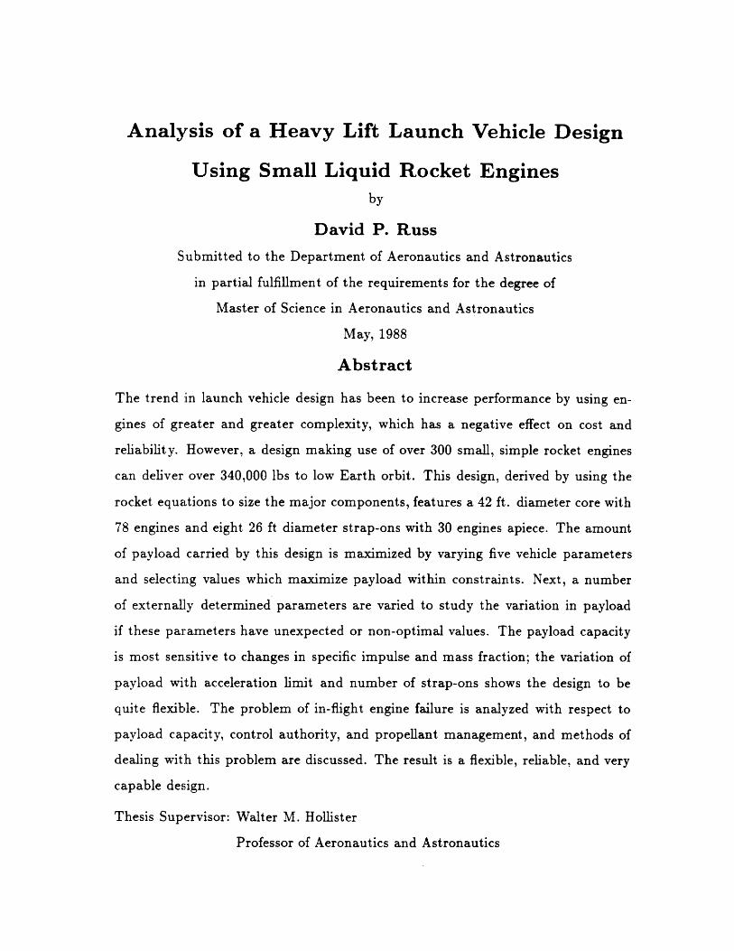
Analysis of a Heavy Lift Launch Vehicle Design
Using Small Liquid Rocket Enginesby
David P. RussSubmitted to the Department of Aeronautics and Astronautics
in partial fulfillment of the requirements for the degree of
Master of Science in Aeronautics and Astronautics
May, 1988
Abstract
The trend in launch vehicle design has been to increase performance by using en-
gines of greater and greater complexity, which has a negative effect on cost and
reliability. However, a design making use of over 300 small, simple rocket engines
can deliver over 340,000 lbs to low Earth orbit. This design, derived by using the
rocket equations to size the major components, features a 42 ft. diameter core with
78 engines and eight 26 ft diameter strap-ons with 30 engines apiece. The amount
of payload carried by this design is maximized by varying five vehicle parameters
and selecting values which maximize payload within constraints. Next, a number
of externally determined parameters are varied to study the variation in payload
if these parameters have unexpected or non-optimal values. The payload capacity
is most sensitive to changes in specific impulse and mass fraction; the variation of
payload with acceleration limit and number of strap-ons shows the design to be
quite flexible. The problem of in-flight engine failure is analyzed with respect to
payload capacity, control authority, and propellant management, and methods of
dealing with this problem are discussed. The result is a flexible, reliable, and very
capable design.
Thesis Supervisor: Walter M. Hollister
Professor of Aeronautics and Astronautics
Preface
The idea for using a large number of small, simple liquid rocket engines for a heavy-
lift launch vehicle is not original to the author. As near as I can tell, the idea
came from Paul Visher, a vice president with Space and Communications Group of
Hughes Aircraft. This has formed the basis for a whole new enterprise for Hughes:
launch vehicle design. The design presented below is sufficiently different from the
Hughes design so that it does not infringe on any proprietary data, but it does share
most of the key advantages of the Hughes concept.
The author would like to thank the following people and institutions for their
invaluable support.
* MIT, and especially Professor Hollister and John Martucelli, director of the
Engineering Internship Program. The EIP placed me here, and I am deeply
grateful.
* The staff of the Hughes Co-op Office (especially Mimi Shefrin) and Dr. John
Drebinger. They, too, have provided key support.
* Chuck Rubin and Dave Knauer, the leaders of the current Hughes launch
vehicle effort. They have trusted me enough to give me an interesting position.
* My family-mother, father, and brother-who looked at early drafts and pro-
vided moral support. They, and the faith in God that they helped to impart,
have kept me going.
El Segundo, CA
December, 1987
Contents
1 Introduction 6
2 Concept Definition
2.1 Reference Mission ....
2.2 Propulsive Capacity
2.2.1 Actual AV
2.'2.2 Drag AV ....
2.2.3 Gravity AV . . .
2.3 Rocket Equations ....
2.4 Initial Design ......
2.4.1 Engine Selection
2.4.2 Strap-on Design
2.4.3 Propellant Tanks
8
8
8
9
..... ...10
..... ...12. . . . . . 13
..... . .15
..... . .15
..... . 15...... .20
3 Performance Analysis
3.1 Performance Analysis Background
3.1.1 The Trajectory Simulator .
3.1.2 Vehicle Assumptions . . . .
3.:1.3 Analysis Methodology . . .
3.2 Trade Studies ............
3.2.1 Liftoff Weight.
27
27
27
28
32
32
32
4
......................................
...................
...................
...................
...................
...................
...................
.....................................
......................................
...................
...................
...................
...................
3.2.2 Core/Strap-on Size Ratio . .
3.:2.3 Core/Strap-on Engine Ratio .
3.2.4 Acceleration Limit ......
3.2.5 Core Shutdown Time .
3.2.6 Trade Study Summary ....
3.3 Variation Studies ...........
3.:3.1 Mass Fraction . . . . . . . . .
3.:3.2 Drag . . . . . . . . . . . . . .
3.:3.3 Number of Strap-ons . . . . .
3.3.4 Specific Impulse .......
3.:3.5 Variation Study Summary . .
3.4 T:rajectory Description .......
4 Engine Failure
4.1 Overview.
4.2 Payload Capability ...........
4.3 Control.
4.3.1 Nominal Control ........
4.3.2 Control with Failed Engines . .
4.3.3 Control Summary .......
4.4 Propellant Consumption Management
4.5 Engine Failure Summary........
5 Conclusion
Bibliography
5
................. . ..34
. . . . . . . . . . . . . . . . . . 36
. . . . . . . . . . . . . . . . . . . 38
. . . . . . . . . . . . . . . . . . 40
. . . . . . . . . . . . . . . . . . .42
. . . . . . . . . . . . . . . . . . .42
. . . . . . . . . . . . . . . . . . .42
. . . . . . . . . . . . . . . . . . . 43
. . . . . . . . . . . . . . . . . . 45
. . .......... . ... . . . . . . . . . . . 47
. . . . . . . . . . . . . . . . . . .47
.. 49
57
57
58
60
60
62
64
65
66
68
70
................................
................
................
................
................
................
................
Chapter 1
Introduction
The problems of getting payload from the Earth's surface into space have intrigued
many people during the course of the 20th century. The past 30 years have seen
advancement in this field that is more rapid than most other technological fields.
Launch vehicles are now available that can place tens of thousands of pounds into
low Earth orbit (LEO) and thousands of pounds into geosynchronous Earth orbit
(GEO). The two major problems with such vehicles continue to be cost and reli-
ability. There is no other form of transportation that costs thousands of dollars
per pound delivered; modern launch vehicles have costs that are the equivalent of
mailing a letter for $2501. And tremendous reliability is required since the payloads
themselves may be worth millions or billions of dollars.
One key area of booster design is engine selection. The choice of engines affects
the perforn:lance, cost, and reliability of a launch vehicle in a fundamental way. Up
until now, the main focus of engine development has been to develop engines that
have great performance. The Space Shuttle Main Engines (SSME's) are a prime
example of this. They have a specific impulse (Ip) of 455 seconds in a vacuum,
among the highest ever achieved by a rocket engine, and are capable of producing
375,000 pounds (1,670,000 N) of thrust apiece at sea level [1, page A-53]. But,
1 Based on a launch cost of $4000/lb for the Titan IV and a one ounce letter.
6
they are extremely expensive and can only be flown for a few flights before a major
overhaul. Even with this expense, an engine was shut down in flight.
Thus one item that is needed to build a low-cost heavy lift launch vehicle is a low-
cost, reliable engine of good performance. An example of this is the RL10, developed
by Pratt and Whitney and currently used on the Centaur upper stage. This engine
has a vacuum I1 p of 440 sec. and has had no in-flight failures in 220 flight firings
[12]. The engine is simple, with a complexity similar to that of a helicopter turbine
engine. The only drawback is that this engine produces 15,000 lbs (67,000 N) of
thrust at sea level; in other words, an average launch vehicle would need around 50
such engines to get off of the ground. Ignoring this drawback for a moment, the
demonstrated reliability of 0.9984 and the possibility of mass production force one
to consider a design based on this engine.
The purpose of this thesis is to generate a design using an uprated version of
this engine., improve the payload capacity by varying many of its parameters, and
address one of the major technical problems with this design, engine failure. This
design could offer a major improvement in launch cost and performance.
7
Chapter 2
Concept Definition
2.1 Reference Mission
The design presented here is that of a heavy lift launch vehicle. The reference
mission, then, will be to take 300,000 lbs (136,000 kg) to a circular low Earth orbit
(LEO) at 100 nautical miles (185 km) altitude based on a due east launch from
Kennedy Space Center. The first step is to use the rocket equations to calculate
the amount of propellant needed. These equations, in turn, require knowledge of
the amount of propulsive AV the launch vehicle must provide.
2.2 Propulsive Capacity
Consider the dynamics of a vehicle in flight at velocity i at an angle 7 to the local
horizontal, as in figure 2.1. The vehicle has mass m, produces a thrust T with a
certain specific impulse (I,p), and experiences a drag D.
These forces can be expressed in the following equation [3, page 323]:
dm Ddu = -gp-- d - g sin ydt (2.1)
m m
where T and D represent the magnitude of these forces resolved in the u direction.
8
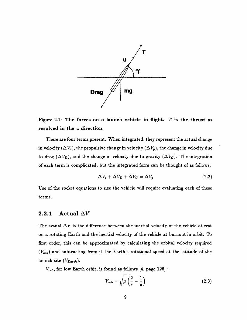
TU
mg
Figure 2.1: The forces on a launch vehicle in flight. T is the thrust as
resolved in the u direction.
There are four terms present. When integrated, they represent the actual change
in velocity (AV.), the propulsive change in velocity (AVp), the change in velocity due
to drag (AVD), and the change in velocity due to gravity (AVG). The integration
of each term is complicated, but the integrated form can be thought of as follows:
iAV + VD + AVG = AVp (2.2)
Use of the rocket equations to size the vehicle will require evaluating each of these
terms.
2.2.1 Actual AV
The actual AV is the difference between the inertial velocity of the vehicle at rest
on a rotating Earth and the inertial velocity of the vehicle at burnout in orbit. To
first order, this can be approximated by calculating the orbital velocity required
(Vob) and subtracting from it the Earth's rotational speed at the latitude of the
launch site (VErth).
Vob, for low Earth orbit, is found as follows [4, page 126]:
V.,b = P(r a) (2.3)
9
where pi is G (mEarth, the gravitational constant times the mass of the Earth, r is the
distance of the body in orbit from the center of the Earth, and a is the semi-major
axis of the orbit.
For a circular orbit, r = a, and assuming the body is- at 185 km altitude,
Vo b 398601. 6378 + 185) = 7793 /sec
or 25,570 ft/sec.
VErth at the equator is found as follows:
27rr 2 r 6378VEarth = - = 2460 = 464 m/sec (2.4)t 24 60 60
or 1520 ft/sec. At other latitudes, this is reduced by a cosine factor. The latitude
of Kennedy Space Center is 28.50, giving
VEath = 464 cos L = 464 cos(28.5) = 408 m/sec
or 1340 ft/sec.
Thus, zAVa is approximately 7385 m/sec or 24,230 ft/sec.
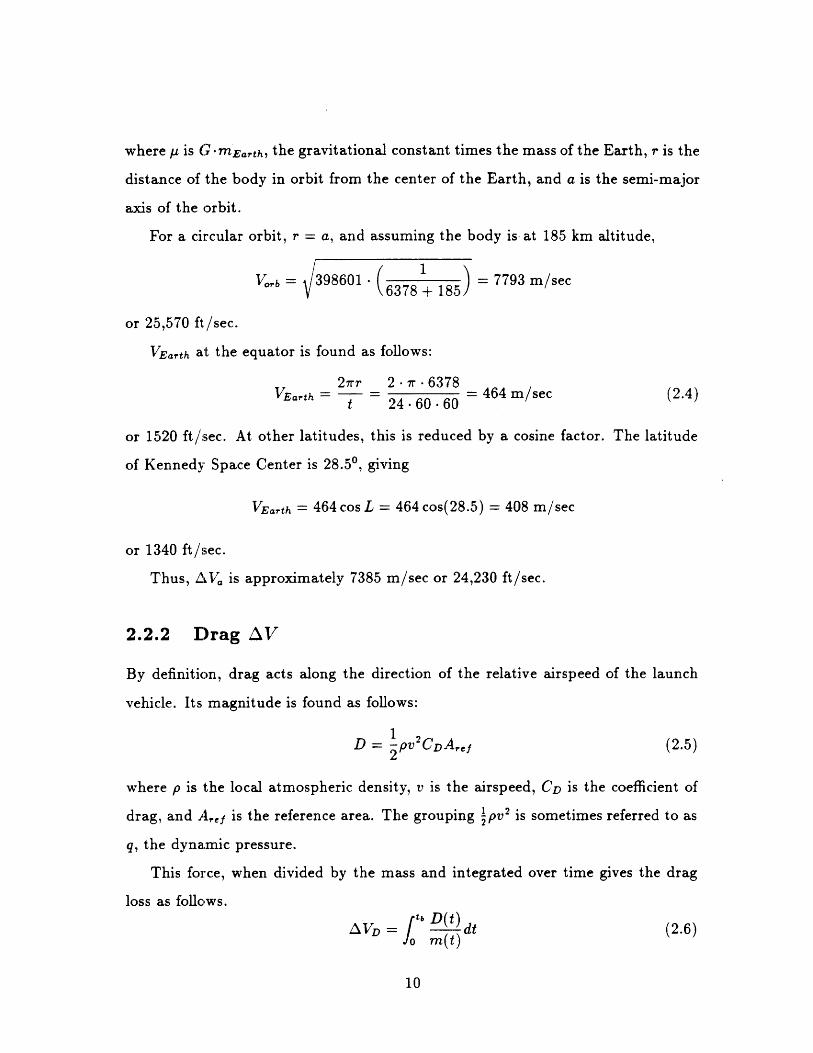
2.2.2 Drag AV
By definition, drag acts along the direction of the relative airspeed of the launch
vehicle. Its magnitude is found as follows:
1D = pv2CDA,rf (2.5)
2
where p is the local atmospheric density, v is the airspeed, CD is the coefficient of
drag, and A,r is the reference area. The grouping 1pv2 is sometimes referred to as
q, the dynamic pressure.
This force, when divided by the mass and integrated over time gives the drag
loss as follows.
ŽAVD = 1t ( ) dt (2.6)fo i"~m t)
10
---
N-
J 600
U
2o( 200z0
f
in 400al
n 200Az0a 2tZ
)-L
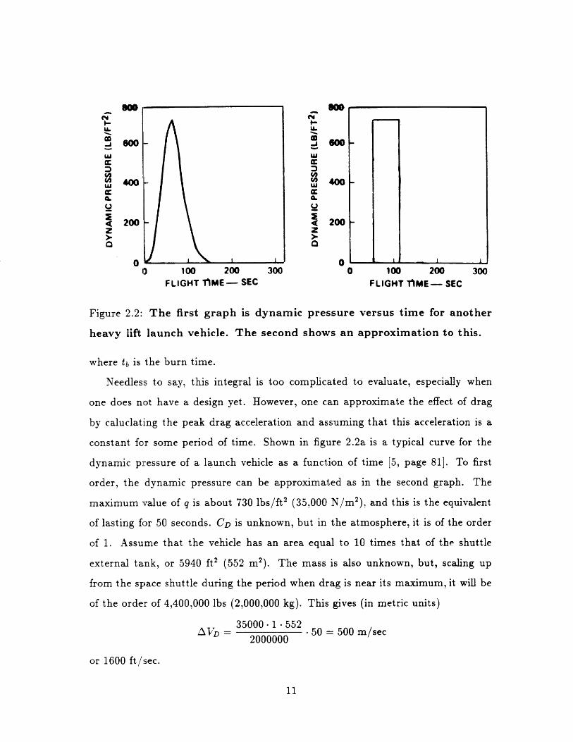
0 100 200 300 0 100 200 300FLIGHT T'ME- SEC FLIGHT tIME- SEC
Figure 2.2: The first graph is dynamic pressure versus time for another
heavy lift launch vehicle. The second shows an approximation to this.
where tb is the burn time.
Needless to say, this integral is too complicated to evaluate, especially when
one does not have a design yet. However, one can approximate the effect of drag
by caluclating the peak drag acceleration and assuming that this acceleration is a
constant for some period of time. Shown in figure 2.2a is a typical curve for the
dynamic pressure of a launch vehicle as a function of time [5, page 81]. To first
order, the dynamic pressure can be approximated as in the second graph. The
maximum value of q is about 730 lbs/ft 2 (35,000 N/m2), and this is the equivalent
of lasting for 50 seconds. CD is unknown, but in the atmosphere, it is of the order
of 1. Assume that the vehicle has an area equal to 10 times that of the shuttle
external tank, or 5940 ft2 (552 m2). The mass is also unknown, but, scaling up
from the space shuttle during the period when drag is near its maximum, it will be
of the order of 4,400,000 lbs (2,000,000 kg). This gives (in metric units)
35000.1 552D 2000000 v50 = 500 m/sec
or 1600 ft/sec.
11
.I I W- L
2.2.3 Gravity AV
For a short thrust period t, and neglecting drag, one can integrate equation 2.1 to
obtain [3, page 324]:
AVG = g t sin y
Over the course of a flight of duration tb, this can be approximated as
AVG - g9 t sin (2.7)
where sin 7 is the integrated average value of sin y over the burn.
This sin has some physical meaning. To first order, it is the time averaged
value of sin y, where y is as defined in figure 2.1. Launch vehicles launch straight
upward (y = 900) initially. When in a circular orbit, = 0°. Assuming that the
launch vehicle pitches over as soon as possible so as to minimize g losses, more time
is spent at lower values of y. 300 is a reasonable estimate.
t b is approximated as follows:
tb - mrnpo (2.8)rh
where mp, op is the propellant mass and rh is the mass flow rate. Given that T is the
thrust and I is the specific impulse, and using the definition of specific impulse,
one obtainsT Ttb
I = = (2.9)rhg mporg
To stay in the air, T > mpg, so tb < I,p for any single stage. For a two stage
vehicle, each stage having t b = Ip, this gives tb = I,p overall. The overall I,p of
the liquid hydrogen/liquid oxygen propulsion is around 400 sec., giving
AVG = 9.8 -400 sin 300 = 1960 m/sec
or 6430 ft/sec.
Thus, the approximations above lead to
AVp = 7385 + 500 + 1960 = 9850 m/sec = 32,300 ft/sec (2.10)
This propulsive AV is used in the rocket equations to size the vehicle.
12
2.3 Rocket Equations
The mass of a launch vehicle can be broken up into three categories [3, page 328]:
mpay, the mass of the payload,
mp,,p, the mass of the propellant burned, and
mt,,rc, the mass of the structure and everything else (e.g., residual propellant,
avionics, etc.).
The sum of these is mo, the total liftoff mass. There are two ratios, defined as
follows:
1 = (2.11)mpay + mpop + mrtruc mO
mtruce = ---- - (2.12)
mrstruc + mpop
The ratio E is referred to as the mass fraction.
In addition, define the exponent k as follows:
k =AV (2.13)cn
where c is gIp for each stage and n is the number of stages.
For the entire vehicle (assuming stages of equal I,p and ) [3, page 333]
A nln (1/R)'/" 1c = e[(1/)l/n" - 1] + 1
This can be solved for as follows:
z (1 -eek ) (2.14)
AVp is known to be 9850 m/sec from above. is unknown, but is of the order of 0.1
[3, page 329] 1. This formula allows one to calculate the inverse of the mass ratio
1 The graph in Hill shows that 0.05 is a good estimate, so 0.1 is conservative.
13
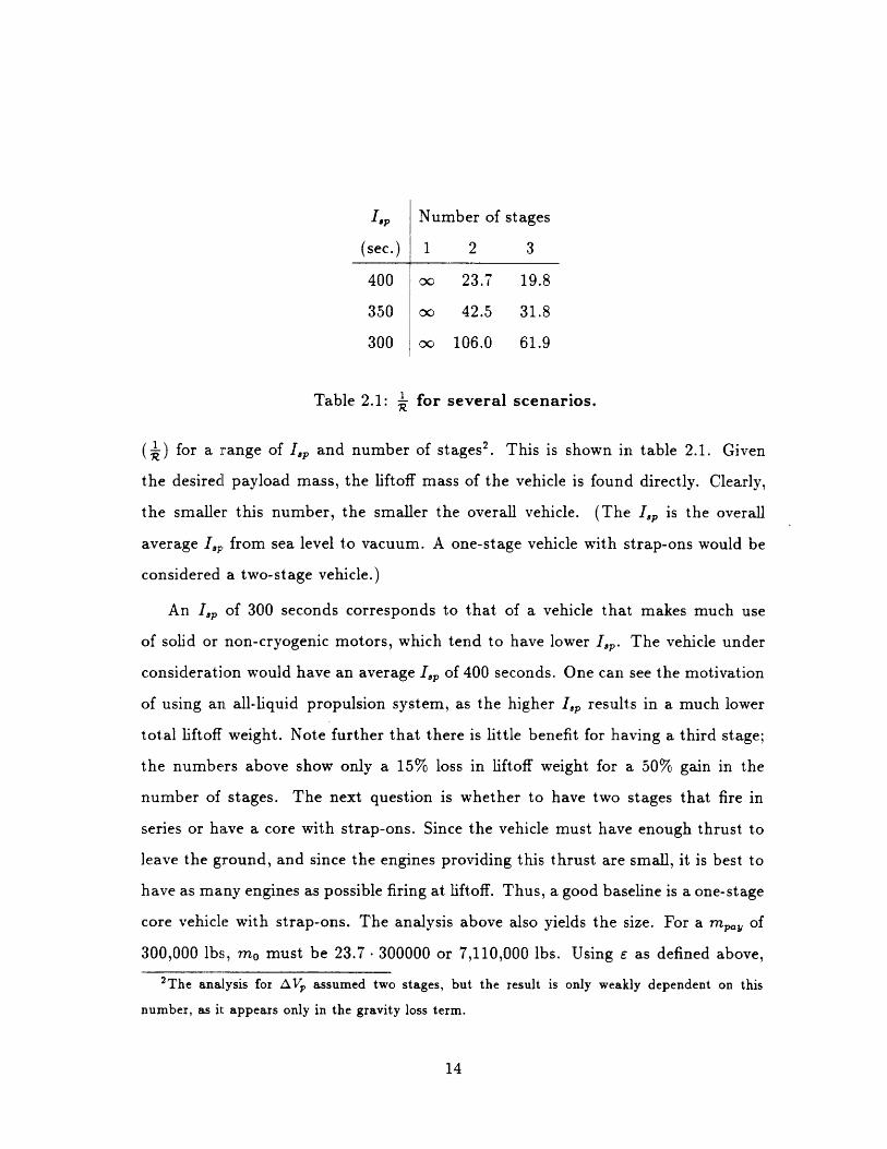
"ap
(sec.)
400
350
300
Number of stages
1 2 3
00 23.7 19.8
00 42.5 31.8
oc 106.0 61.9
Table 2.1: for several scenarios.
(~) for a range of I and number of stages2 . This is shown in table 2.1. Given
the desired payload mass, the liftoff mass of the vehicle is found directly. Clearly,
the smaller this number, the smaller the overall vehicle. (The I is the overall
average I,, from sea level to vacuum. A one-stage vehicle with strap-ons would be
considered a two-stage vehicle.)
An I of 300 seconds corresponds to that of a vehicle that makes much use
of solid or non-cryogenic motors, which tend to have lower I,,. The vehicle under
consideration would have an average I,, of 400 seconds. One can see the motivation
of using an all-liquid propulsion system, as the higher I, results in a much lower
total liftoff weight. Note further that there is little benefit for having a third stage;
the numbers above show only a 15% loss in liftoff weight for a 50% gain in the
number of stages. The next question is whether to have two stages that fire in
series or have a core with strap-ons. Since the vehicle must have enough thrust to
leave the ground, and since the engines providing this thrust are small, it is best to
have as many engines as possible firing at liftoff. Thus, a good baseline is a one-stage
core vehicle with strap-ons. The analysis above also yields the size. For a mpa of
300,000 lbs, m0 must be 23.7* 300000 or 7,110,000 lbs. Using E as defined above,2 The analysis for AVp assumed two stages, but the result is only weakly dependent on this
number, as it appears only in the gravity loss term.
14
this gives a structural mass of 681,000 lbs and a propellant mass of 6,129,000 lbs.
2.4 Initial Design
2.4.1 Engine Selection
Obviously, a major constraint on launch vehicles is that they must get off the ground.
In numeric terms, this means that the thrust must be greater than the weight. Let
us assume that the thrust to weight ratio is 1.2 at liftoff, giving a takeoff thrust of
8,532,000 lbs at sea level. Regardless of the choice of small thrust engine, one is
going to need hundreds of engines firing at liftoff. If the engines have a thrust of
10,000 lbs apiece, one will need 854 engines; even if the thrust is as great as 100,000
lbs, one will still need 86 engines.
The aforementioned RL10 has a vacuum thrust around 16,500 lbs (73,400 N).
However, Pratt and Whitney has conducted a study which concluded that this
engine can easily be uprated to 27,000 lbs (120,100 N) of sea level thrust while
manintaining the simplicity needed for mass production [2]. This engine, referred
to as the RL1OJ, will be used as the baseline engine for this design. Liftoff would
require at least 316 such engines.
An efficient scheme for mounting these engines is to mount the engines in clus-
ters. From the standpoint of controls and plumbing, each cluster can be treated as
a single engine. The RL10 has flown in clusters of 6 on early versions of the S-IV
stage, so the engines in this design will be mounted in clusters of 6. Thus, the initial
design will rely on 318 RL1OJ engines.
2.4.2 Strap-on Design
There are a number of possibities for strap-on size and engine placement. For each
possibility, there are ways of using the same design with fewer than the maximum
possible number of strap-ons. For example, if one had an eight strap-on design,
15
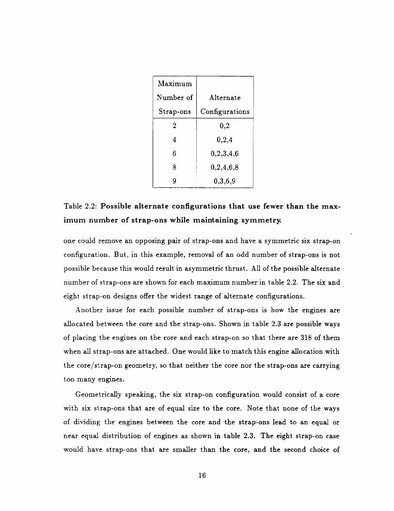
Table 2.2: Possible alternate configurations that use fewer than the max-
imum number of strap-ons while maintaining symmetry.
one could remove an opposing pair of strap-ons and have a symmetric six strap-on
configuration. But, in this example, removal of an odd number of strap-ons is not
possible because this would result in asymmetric thrust. All of the possible alternate
number of strap-ons are shown for each maximum number in table 2.2. The six and
eight strap-on designs offer the widest range of alternate configurations.
Another issue for each possible number of strap-ons is how the engines are
allocated between the core and the strap-ons. Shown in table 2.3 are possible ways
of placing the engines on the core and each strap-on so that there are 318 of them
when all strap-ons are attached. One would like to match this engine allocation with
the core/strap-on geometry, so that neither the core nor the strap-ons are carrying
too many engines.
Geometrically speaking, the six strap-on configuration would consist of a core
with six strap-ons that are of equal size to the core. Note that none of the ways
of dividing the engines between the core and the strap-ons lead to an equal or
near equal distribution of engines as shown in table 2.3. The eight strap-on case
would have strap-ons that are smaller than the core, and the second choice of
16
Maximum
Number of Alternate
Strap-ons Configurations
2 0,2
4 0,2,4
6 0,2,3,4,6
8 0,2,4,6,8
9 0,3,6,9
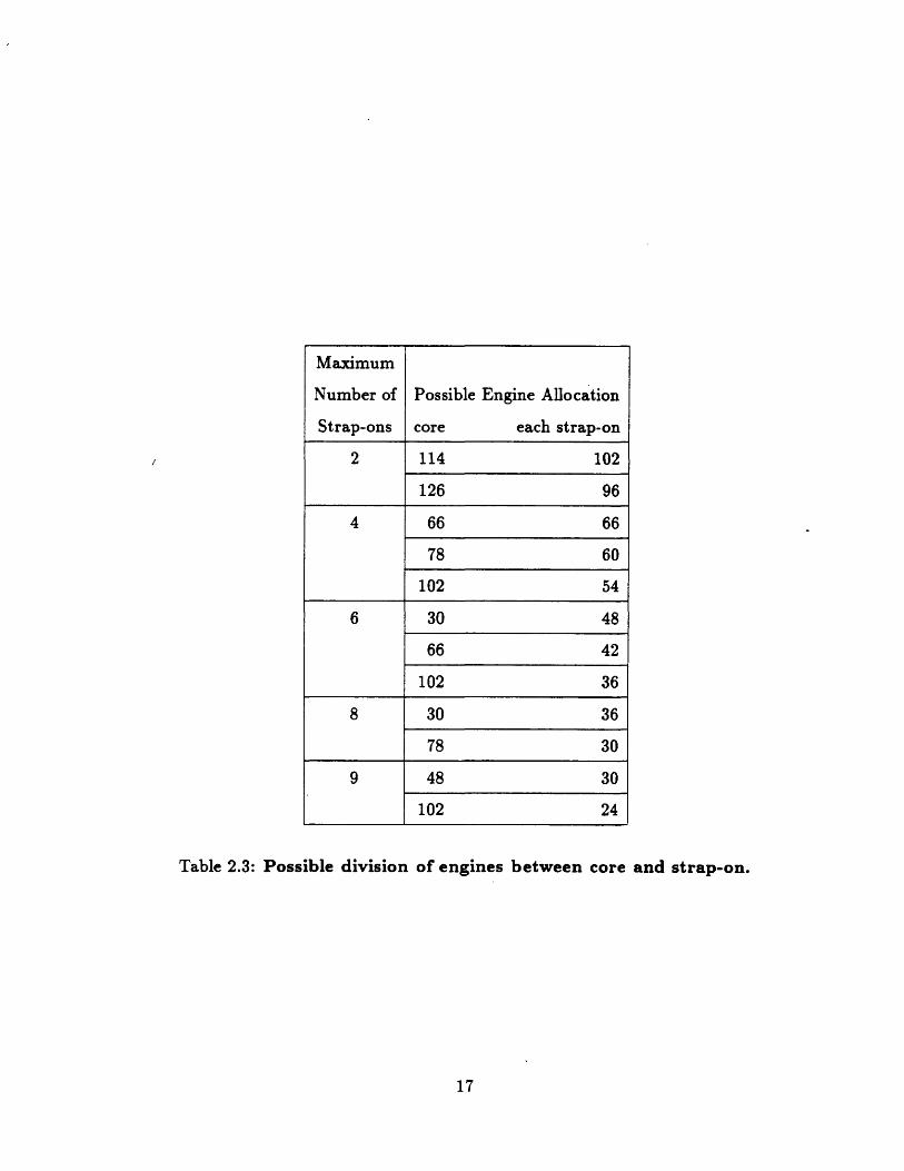
Table 2.3: Possible division of engines between core and strap-on.
17
Maximum
Number of Possible Engine Allocation
Strap-ons core each strap-on
2 114 102
126 96
4 66 66
78 60
102 54
6 30 48
66 42
102 36
8 30 36
78 30
9 48 30
102 24
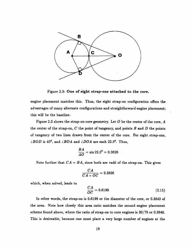
Figure 2.3: One of eight strap-ons attached to the core.
engine placement matches this. Thus, the eight strap-on configuration offers the
advantages of many alternate configurations and straightforward engine placement;
this will be the baseline.
Figure 2.3 shows the strap-on-core geometry. Let O be the center of the core, A
the center of the strap-on, C the point of tangency, and points B and D the points
of tangency of two lines drawn from the center of the core. For eight strap-ons,
LBOD is 450, and LBOA and LDOA are each 22.50. Thus,
BA- = sin 22.50 = 0.3826AO
Note further that CA = BA, since both are radii of the strap-on. This gives
CA=CA 0.3826CA+OC
which, when solved, leads toCA
= 0.6199 (2.15)OC
In other words, the strap-on is 0.6199 or the diameter of the core, or 0.3843 of
the area. Note how closely this area ratio matches the second engine placement
scheme found above, where the ratio of strap-on to core engines is 30/78 or 0.3846.
This is desireable, because one must place a very large number of engines at the
18
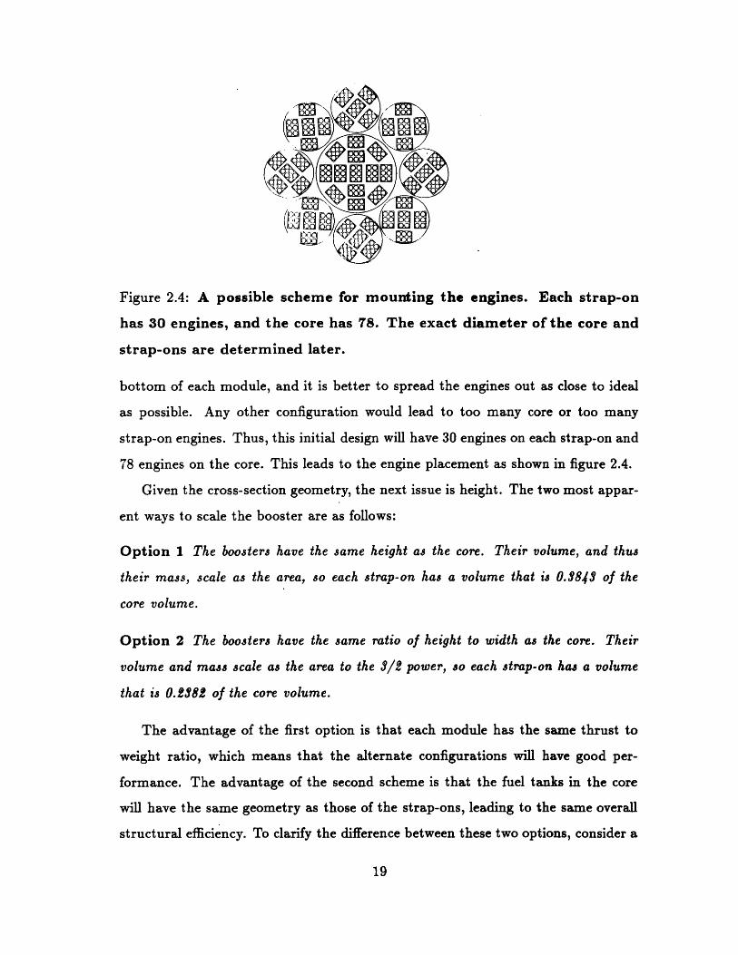
Figure 2.4: A possible scheme for mounting the engines. Each strap-on
has 30 engines, and the core has 78. The exact diameter of the core and
strap-ons are determined later.
bottom of each module, and it is better to spread the engines out as close to ideal
as possible. Any other configuration would lead to too many core or too many
strap-on engines. Thus, this initial design will have 30 engines on each strap-on and
78 engines on the core. This leads to the engine placement as shown in figure 2.4.
Given the cross-section geometry, the next issue is height. The two most appar-
ent ways to scale the booster are as follows:
Option 1 The boosters have the same height as the core. Their volume, and thus
their mass, scale as the area, so each strap-on has a volume that is 0.$843 of the
core volume.
Option 2 The boosters have the same ratio of height to width as the core. Their
volume and mass scale as the area to the 3/2 power, so each strap-on has a volume
that is 0.2382 of the core volume.
The advantage of the first option is that each module has the same thrust to
weight ratio, which means that the alternate configurations will have good per-
formance. The advantage of the second scheme is that the fuel tanks in the core
will have the same geometry as those of the strap-ons, leading to the same overall
structural efficiency. To clarify the difference between these two options, consider a
19
Table 2.4: Liftoff weight comparison of strap-on height options.
launch of a two strap-on alternate configuration. Given the volume ratios and the
overall propellant mass, one can allocate mprop between the core and the strap-ons.
Given , one can then solve for mstruc, as
mstruc
These lead to the results of table 2.4, neglecting the payload weight. The huge
core of option 2 is a large burden when fewer than the maximum number of strap-ons
is used, leading to the selection of option 1 as the initial baseline.
2.4.3 Propellant Tanks
Launch vehicles have been described as 'flying gas tanks' and from the numbers
above, it is not difficult to see why. The primary structural element of launch
vehicles is the tankage.
The propellant for this launch vehicle consists of liquid hydrogen and liquid
oxygen. Hydrogen boils at -252.90 C (200 K) and has a density of 4.42 lb/ft3 (70.8
kg/m3). Oxygen boils at -183.00 C (900 K) and has a density of 71.2 lb/ft3 (1140
kg/m3). The conditions in the tanks will almost certainly be near boiling and this,
combined with the need to force out large amounts of propellant, means that these
tanks are also pressure vessels. This is one of the main reasons why propellant tanks
20
Option 1 Option 2
Core propellant 1,504,270 lbs 2,109,380 lbs
Core structure 167,140 lbs 234,380 lbs
Strap-on propellant 578,090 lbs 502,450 lbs
Strap-on structure 64,230 lbs 55,380 lbs
Liftoff Weight (2 strap-ons) 2,956,010 lbs 3,460,320 lbs
tend to have hemispherical or ellipsoidal end caps.
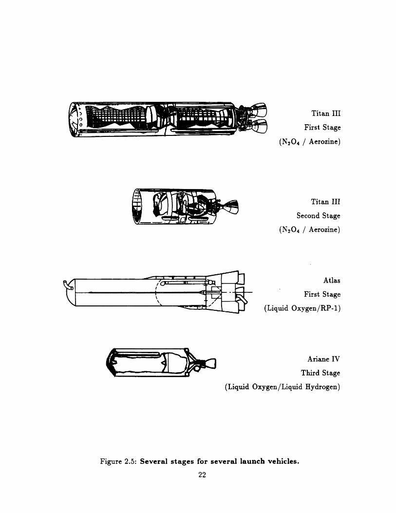
Figure 2.5 shows several existing tank configurations. [6, page I-3] [7, page 1-2]
[8, fig. 1.6] In all cases, the tanks show the rounded end caps. Note that most of
these tanks are 'long and skinny'; that is, they have round caps with long cylindrical
barrel sections. In almost all of these cases, only a few engines had to be placed
at the base of the vehicle and so, given transportation restrictions, the vehicles
tend to be narrow. An exception is the integral tank shown on the Ariane. In this
case, the smaller tank is made with a common bulkhead to the larger tank. The
disadvantages of such a configuration is that it complicates the propellant feed and
requires extensive insulation between the hydrogen and oxygen [8, page A1.13].
The RL1OJ uses a mixture ratio of 6:1, oxygen to hydrogen. This partially offsets
the density difference shown above, and the hydrogen tank will be 2.68 times the
volume of the oxygen tank. Thus, the hydrogen tank will consist of end caps and
a barrel, and the diameter of the barrel will be sized by the oxygen tank. If the
hydrogen tank is narrow enough, the oxygen tank will also be a capped cylinder.
If the hydrogen tank is too wide, one will have an integral tank and/or a tank
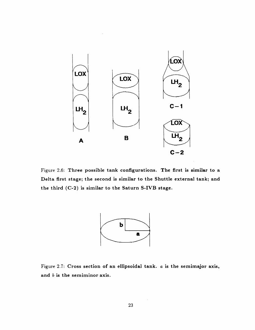
configuration that necks down. Figure 2.6 shows the three basic possibilities. One
has to place 30 or 78 engines at the base of the stage, so the tank configuration
must be of the second or third type, because these are wider than the first. Of
course, the strap-ons and core do not have to have the same configuration. As a
first try, the strap-on will use the second configuration, and the core will use either
the second or third as necessary.
The strap-on contains 578,090 lbs of propellant. This corresponds to 495,510 lbs
of liquid oxygen, or 6963 ft3 . Assume that the tank consists of two ellipsoidal caps
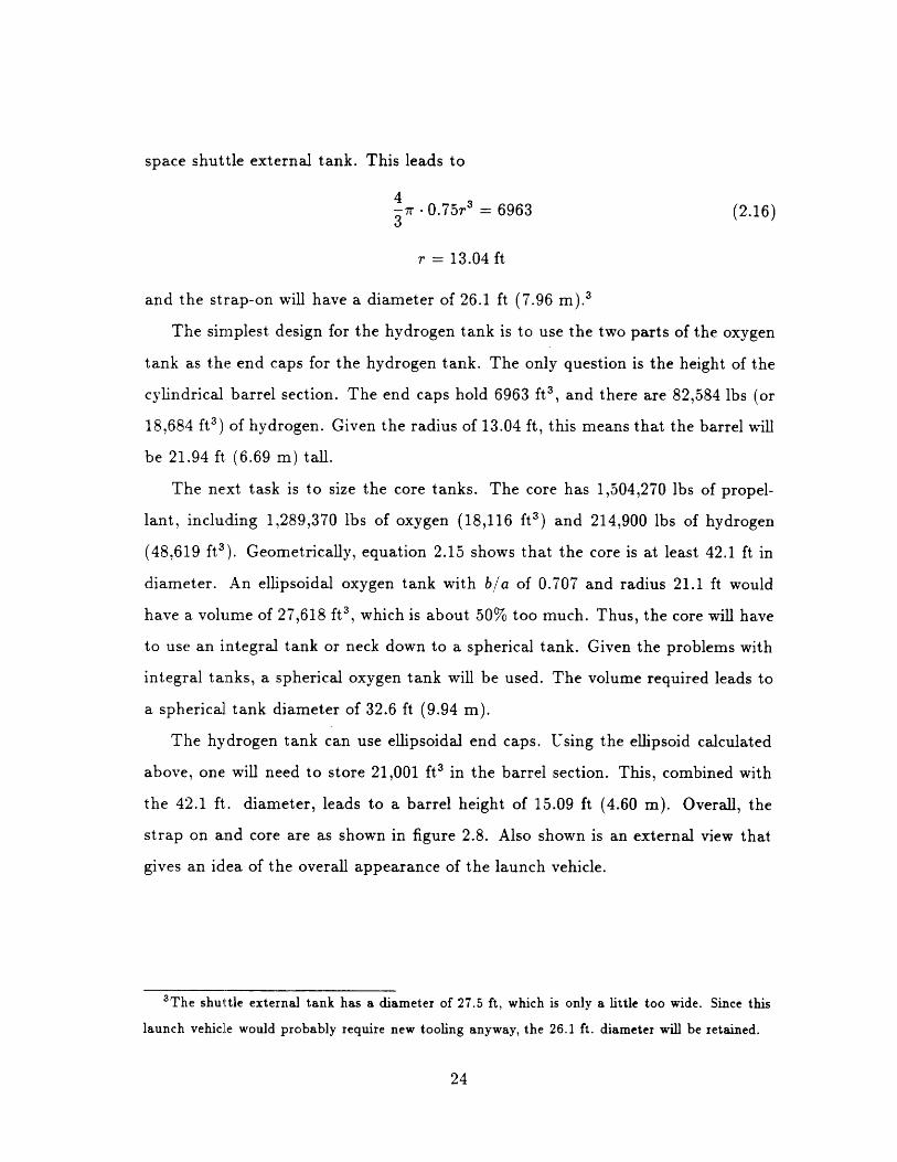
welded together. Figure 2.7 shows the geometry. An ellipsoidal pressure vessel can-
not have a ratio b/a of less than V'/2, or the structure will experience compression
near its equator, leading to buckling [9, page 28]. Assume that b/a is 0.75, like the
21
Titan III
First Stage
(N2 04 / Aerozine)
Titan III
Second Stage
(N204 / Aerozine)
Atlas
First Stage
(Liquid Oxygen/RP-1)
Ariane IV
Third Stage
(Liquid Oxygen/Liquid Hydrogen)
Figure 2.5: Several stages for several launch vehicles.
22
e�T�p
LOXY
Xj
LH2C-I
A B
C-2
Figure 2.6: Three possible tank configurations. The first is similar to a
Delta first stage; the second is similar to the Shuttle external tank; and
the third (C-2) is similar to the Saturn S-IVB stage.
a
Figure 2.7: Cross section of an ellipsoidal tank. a is the semimajor axis,
and b is the semiminor axis.
23
space shuttle external tank. This leads to
4-r ·0.75r3 = 6963 (2.16)3
r = 13.04 ft
and the strap-on will have a diameter of 26.1 ft (7.96 m).3
The simplest design for the hydrogen tank is to use the two parts of the oxygen
tank as the end caps for the hydrogen tank. The only question is the height of the
cylindrical barrel section. The end caps hold 6963 ft3 , and there are 82,584 lbs (or
18,684 ft3 ) of hydrogen. Given the radius of 13.04 ft, this means that the barrel will
be 21.94 ft (6.69 m) tall.
The next task is to size the core tanks. The core has 1,504,270 lbs of propel-
lant, including 1,289,370 lbs of oxygen (18,116 ft3 ) and 214,900 lbs of hydrogen
(48,619 ft3 ). Geometrically, equation 2.15 shows that the core is at least 42.1 ft in
diameter. An ellipsoidal oxygen tank with ba of 0.707 and radius 21.1 ft would
have a volume of 27,618 ft3, which is about 50% too much. Thus, the core will have
to use an integral tank or neck down to a spherical tank. Given the problems with
integral tanks, a spherical oxygen tank will be used. The volume required leads to
a spherical tank diameter of 32.6 ft (9.94 m).
The hydrogen tank can use ellipsoidal end caps. Using the ellipsoid calculated
above, one will need to store 21,001 ft3 in the barrel section. This, combined with
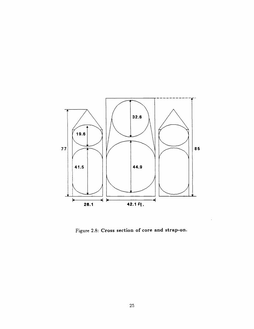
the 42.1 ft. diameter, leads to a barrel height of 15.09 ft (4.60 m). Overall, the
strap on and core are as shown in figure 2.8. Also shown is an external view that
gives an idea of the overall appearance of the launch vehicle.
3 The shuttle external tank has a diameter of 27.5 ft, which is only a little too wide. Since this
launch vehicle would probably require new tooling anyway, the 26.1 ft. diameter will be retained.
24
7'
I-
26.1 42.1 ft ,
Figure 2.8: Cross section of core and strap-on.
25
�5
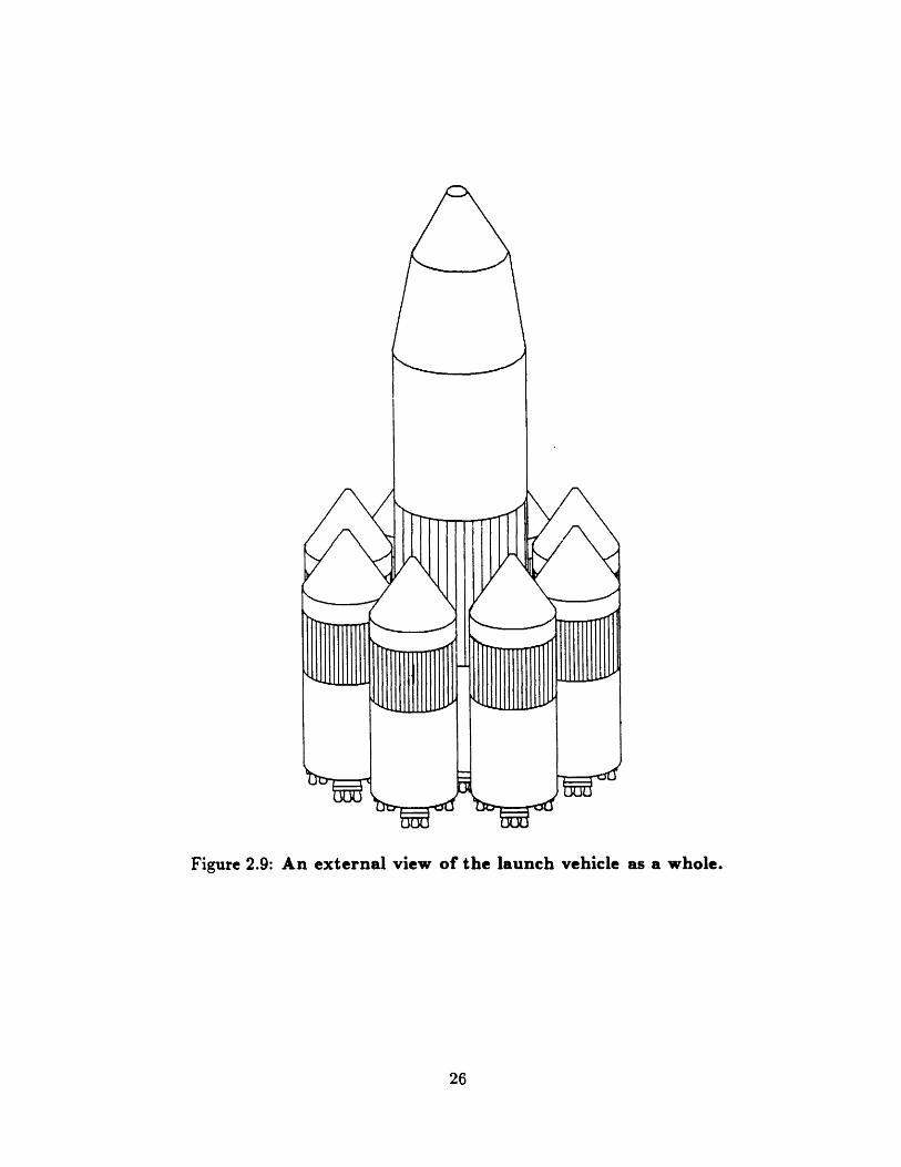
Figure 2.9: An external view of the launch vehicle as a whole.
26
Chapter 3
Performance Analysis
Given a design, the performance of the launch vehicle can be analyzed in detail.
This analysis can be used to improve the design, validate the desired performance,
and identify key operational characteristics of this type of launch vehicle. The per-
formance analysis, in turn, requires an accurate simulator and certain assumptions
about launch vehicle parameters.
3.1 Performance Analysis Background
3.1.1 The Trajectory Simulator
The performance and the trajectory of the launch vehicle were simulated using a
program called PRO-Launch. This programs integrates from flight event to flight
event using a fourth-order Runge-Kutta integrator with fifth-order step size control.
The program takes account of drag with lookup tables of CD vs. Mach Number,
and uses the 1976 U.S. Standard Atmosphere (with no winds) to find atmospheric
properties. The only major flight parameter that is not taken into account is lift,
but given small angles of attack and the fact that the drag (which is taken into
account) will be much larger than any lift, this does not represent much loss in
simulation accuracy.
27
Given a flight simulation, the vehicle must place its payload into a circular orbit
at the desired altitude. The following scheme is employed as a simplified approach to
guidance. The pitch angle at three specific times in the flight is variable. A constant
pitch rate is selected between these angles such that the pitch angle is a continuous
function of time. The program iterates on these three angles until the payload has
been placed into a circular orbit of arbitrary altitude. The only other degree of
freedom is the payload mass, and this is adusted until the payload has been placed
in the desired circular orbit.
The simulator is completely accurate as far as the integration is concerned, but
its pitch profiles are empirically derived. In other words, the program is correct, but
it may not be optimal. This slight loss of optimality is offset by a tremendous gain
in simplicity and ease of use, and this led to the selection of PRO-Launch as the
simulator. Thus, each data point below represents a fully detailed simulation of the
flight of the vehicle.
3.1.2 Vehicle Assumptions
There are many variables that go into a launch vehicle simulation. The following
tables list all of the variables used to simulate the performance. (All of the inputs
into the program are in metric units, so they are listed first.)
Masses:
Component Mass Weight
Core Inert Weight 75813.2 kg 167140 lbs
Fairing Weight 11340.0 kg 25000 lbs
Core Propellant Weight 682325.4 kg 1504270 lbs
Strap-on Inert Weight 29134.2 kg 64230 lbs
Strap-on Propellant Weight 262217.2 kg 578090 lbs
Source: Table 2.4; fairing weight based on Hughes design.
28
3.5
3
20g 2
0
1
0.5
00 2 4 6 8
ach No.
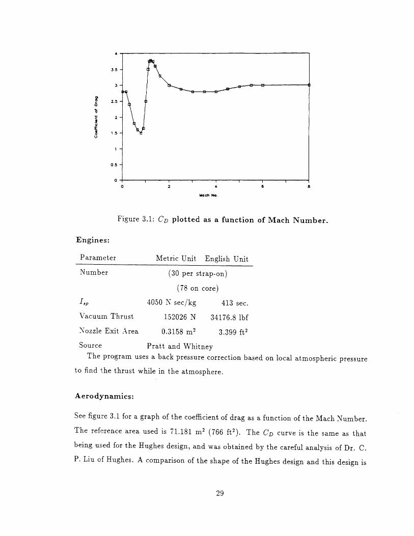
Figure 3.1: CD plotted as a function of Mach Number.
Engines:
Parameter Metric Unit English Unit
Number (30 per strap-on)
(78 on core)
ISP 4050 N sec/kg 413 sec.
Vacuum Thrust 152026 N 34176.8 lbf
Nozzle Exit Area 0.3158 m2 3.399 ft2
Source Pratt and WhitneyThe program uses a back pressure correction based on local atmospheric pressure
to find the thrust while in the atmosphere.
Aerodynamics:
See figure 3.1 for a graph of the coefficient of drag as a function of the Mach Number.
The reference area used is 71.181 m2 (766 ft2). The CD curve is the same as that
being used for the Hughes design, and was obtained by the careful analysis of Dr. C.
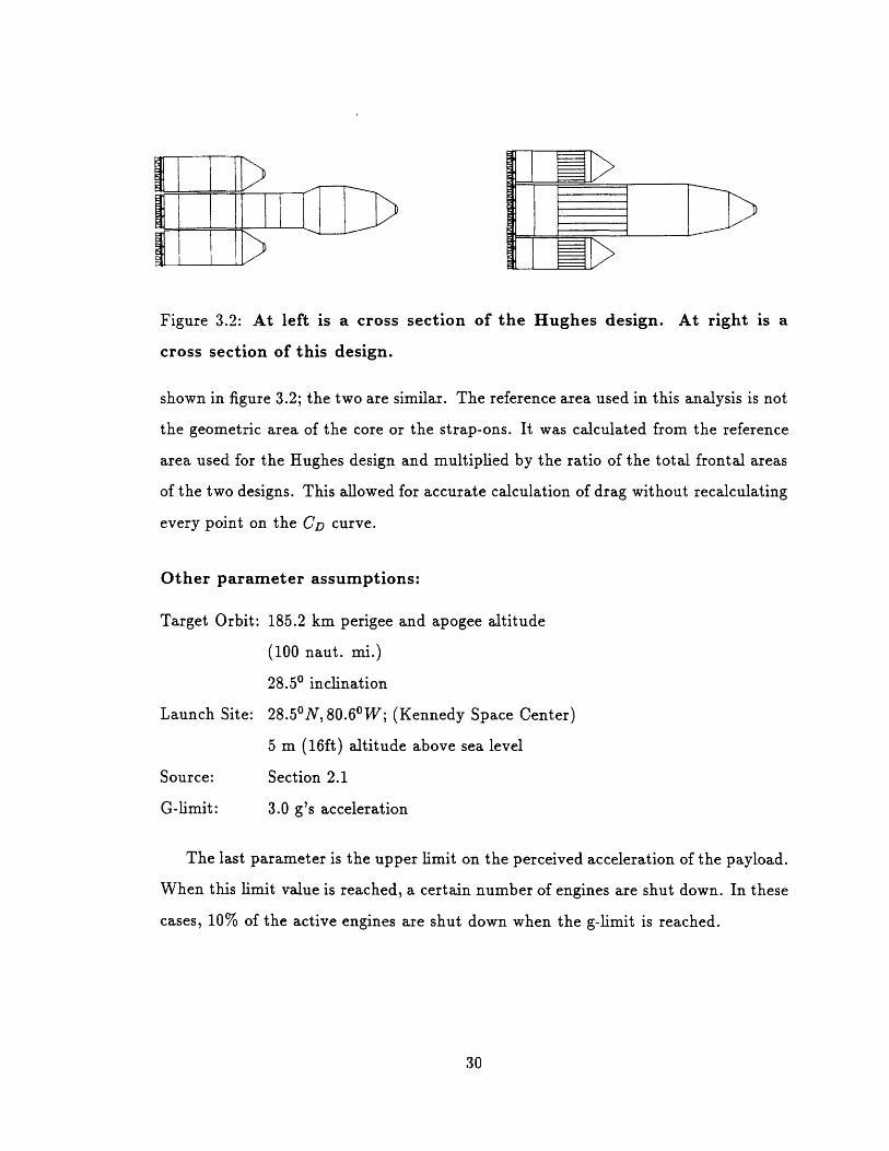
P. Liu of Hughes. A comparison of the shape of the Hughes design and this design is
29
Ii,
\ =LE
Figure 3.2: At left is a cross section of the Hughes design. At right is a
cross section of this design.
shown in figure 3.2; the two are similar. The reference area used in this analysis is not
the geometric area of the core or the strap-ons. It was calculated from the reference
area used for the Hughes design and multiplied by the ratio of the total frontal areas
of the two designs. This allowed for accurate calculation of drag without recalculating
every point on the CD curve.
Other parameter assumptions:
Target Orbit:
Launch Site:
Source:
G-limit:
185.2 km perigee and apogee altitude
(100 naut. mi.)
28.50 inclination
28.50 N, 80.60 W; (Kennedy Space Center)
5 m (16ft) altitude above sea level
Section 2.1
3.0 g's acceleration
The last parameter is the upper limit on the perceived acceleration of the payload.
When this limit value is reached, a certain number of engines are shut down. In these
cases, 10% of the active engines are shut down when the g-limit is reached.
30
i
I
- r s -
__ - = - _= ==-
A | | -
iI�
7 MD
r II I
I I I I/, ,
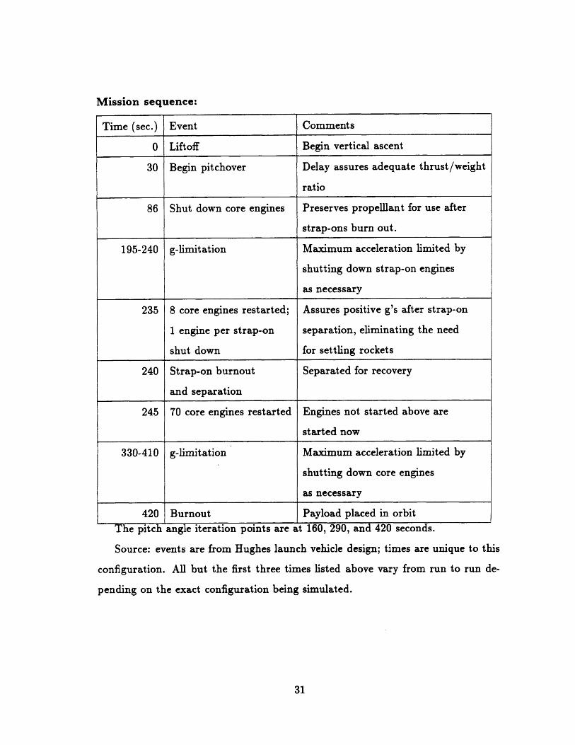
Mission sequence:
Time (sec.) Event Comments
0 Liftoff Begin vertical ascent
30 Begin pitchover Delay assures adequate thrust/weight
ratio
86 Shut down core engines Preserves propellant for use after
strap-ons burn out.
195-240 g-limitation Maximum acceleration limited by
shutting down strap-on engines
as necessary
235 8 core engines restarted; Assures positive g's after strap-on
1 engine per strap-on separation, eliminating the need
shut down for settling rockets
240 Strap-on burnout Separated for recovery
and separation
245 70 core engines restarted Engines not started above are
started now
330-410 g-limitation Maximum acceleration limited by
shutting down core engines
as necessary
420 Burnout Payload placed in orbit
The pitch angle iteration points are at 160, 290, and 420 seconds.
Source: events are from Hughes launch vehicle design; times are unique to this
configuration. All but the first three times listed above vary from run to run de-
pending on the exact configuration being simulated.
31
3.1.3 Analysis Methodology
The procedure for analyzing the payload capacity of this design is as follows. First,
a series of optimizing trade studies will be carried out by varying vehicle parameters
and selecting those values which maximize payload within constraints. These pa-
rameters include liftoff weight, core/strap-on size ratio, core/strap-on engine num-
ber ratio, g-limit, and core shutdown time. Note that each of these parameters
can be chosen in advance by the designer. The end result of this phase will be an
improved vehicle design.
Second, a series of analyses will be carried out which show how the performance
changes when certain other parameters are varied. These other parameters cannot
be chosen by the designer, but may turn out to have values higher or lower than
expected. These parameters include mass fraction (e), drag, number of strap-ons,
and specific impulse (I,p). The end result of this phase will be an understanding of
how 'robust' the design is to changes in externally determined parameters.
This section concludes with a detailed trajectory presentation. (The output of
PRO-Launch is in English units, and all of the results below are tabulated in English
units.)
3.2 Trade Studies
3.2.1 Liftoff Weight
The first parameter that will be varied is the total liftoff weight. For this analysis,
all of the system parameters listed above are held constant except for the masses.
The core and strap-on propellant masses are increased while holding the ratio of
core to strap-on propellant constant. The mass fraction of 0.1 is also held constant,
so the increased propellant masses mean increased structural masses. The results
of this study are presented in table 3.1 and graphed against the total weight in
32
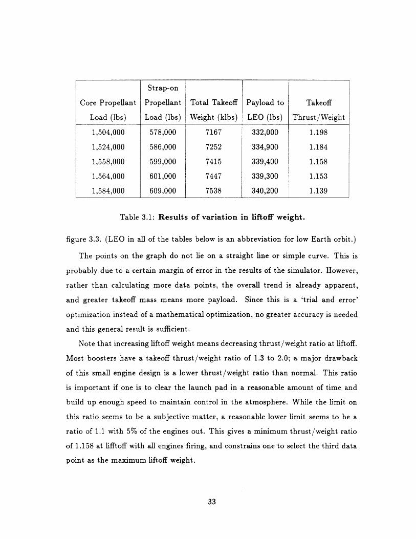
Table 3.1: Results of variation in liftoff weight.
figure 3.3. (LEO in all of the tables below is an abbreviation for low Earth orbit.)
The points on the graph do not lie on a straight line or simple curve. This is
probably due to a certain margin of error in the results of the simulator. However,
rather than calculating more data points, the overall trend is already apparent,
and greater takeoff mass means more payload. Since this is a 'trial and error'
optimization instead of a mathematical optimization, no greater accuracy is needed
and this general result is sufficient.
Note that increasing liftoff weight means decreasing thrust/weight ratio at liftoff.
Most boosters have a takeoff thrust/weight ratio of 1.3 to 2.0; a major drawback
of this small engine design is a lower thrust/weight ratio than normal. This ratio
is important if one is to clear the launch pad in a reasonable amount of time and
build up enough speed to maintain control in the atmosphere. While the limit on
this ratio seems to be a subjective matter, a reasonable lower limit seems to be a
ratio of 1.1 with 5% of the engines out. This gives a minimum thrust/weight ratio
of 1.158 at lifftoff with all engines firing, and constrains one to select the third data
point as the maximum liftoff weight.
33
Strap-on
Core Propellant Propellant Total Takeoff Payload to Takeoff
Load (lbs) Load (lbs) Weight (klbs) LEO (lbs) Thrust/Weight
1,504,000 578,000 7167 332,000 1.198
1,524,000 586,000 7252 334,900 1.184
1,558,000 599,000 7415 339,400 1.158
1,564,000 601,000 7447 339,300 1.153
1,584,000 609,000 7538 340,200 1.139
.;1
:40 -
:538 -:538 -
335 -
:534 -
:333 -
:532-7.15 7.25 7.35 7.45 7.55
Totbl Tokeoff Weight (b.)
Figure 3.3: Payload as a function of liftoff weight.
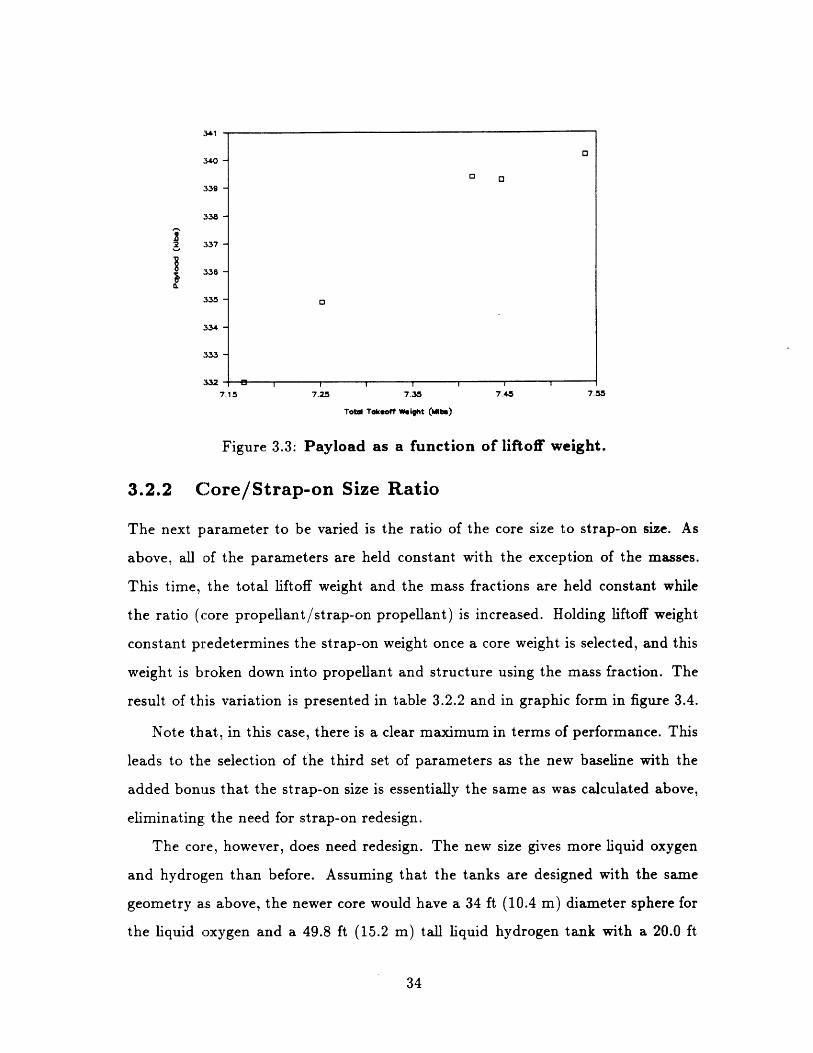
3.2.2 Core/Strap-on Size Ratio
The next parameter to be varied is the ratio of the core size to strap-on size. As
above, all of the parameters are held constant with the exception of the masses.
This time, the total liftoff weight and the mass fractions are held constant while
the ratio (core propellant/strap-on propellant) is increased. Holding liftoff weight
constant predetermines the strap-on weight once a core weight is selected, and this
weight is broken down into propellant and structure using the mass fraction. The
result of this variation is presented in table 3.2.2 and in graphic form in figure 3.4.
Note that, in this case, there is a clear maximum in terms of performance. This
leads to the selection of the third set of parameters as the new baseline with the
added bonus that the strap-on size is essentially the same as was calculated above,
eliminating the need for strap-on redesign.
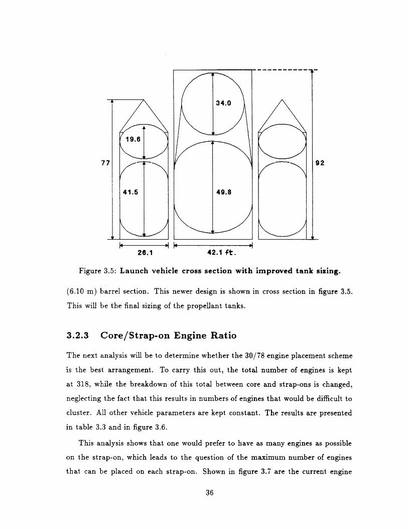
The core, however, does need redesign. The new size gives more liquid oxygen
and hydrogen than before. Assuming that the tanks are designed with the same
geometry as above, the newer core would have a 34 ft (10.4 m) diameter sphere for
the liquid oxygen and a 49.8 ft (15.2 m) tall liquid hydrogen tank with a 20.0 ft
34
0 O
0
_ _ .
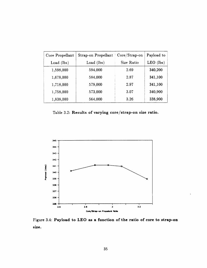
Table 3.2: Results of varying core/strap-on size ratio.
.4.
344
343-
342 -
341-
1 340-
339 -
338-"Iw' -
337 -
336 -
3M-2.8
3.23.22.8 3
Com/strep-a Prop.ket te
Figure 3.4: Payload to LEO as a function of the ratio of core to strap-on
size.
35
ICore Propellant Strap-on Propellant Core/Strap-on Payload to
Load (bs) Load (lbs) Size Ratio LEO (lbs)
1,598,000 594,000 2.69 340,200
1,678,000 584,000 2.87 341,100
1,718,000 579,000 2.97 341,100
1,758,000 573,000 3.07 340,900
1,838,000 564,000 3.26 338,900
.
-
"'
'7
28.1 42.1 ft.
Figure 3.5: Launch vehicle cross section with improved tank sizing.
(6.10 m) barrel section. This newer design is shown in cross section in figure 3.5.
This will be the final sizing of the propellant tanks.
3.2.3 Core/Strap-on Engine Ratio
The next analysis will be to determine whether the 30/78 engine placement scheme
is the best arrangement. To carry this out, the total number of engines is kept
at 318, while the breakdown of this total between core and strap-ons is changed,
neglecting the fact that this results in numbers of engines that would be difficult to
cluster. All other vehicle parameters are kept constant. The results are presented
in table 3.3 and in figure 3.6.
This analysis shows that one would prefer to have as many engines as possible
on the strap-on, which leads to the question of the maximum number of engines
that can be placed on each strap-on. Shown in figure 3.7 are the current engine
36
12
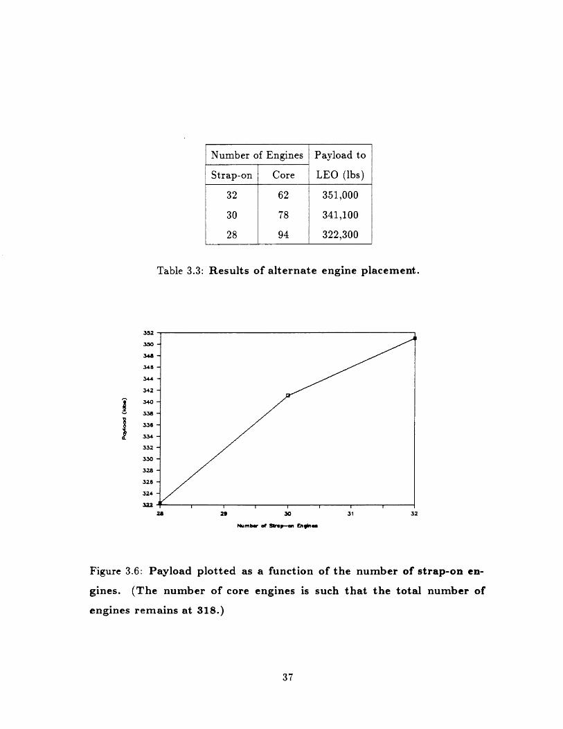
Table 3.3: Results of alternate engine placement.
352
350
348
345
344
342
1 340
336
334
332
330
328
326
324
3228 2 30 31 32
Number of Sbp-a Eginea
Figure 3.6: Payload plotted as a function of the number of strap-on en-
gines. (The number of core engines is such that the total number of
engines remains at 318.)
37
Number of Engines Payload to
Strap-on Core LEO (lbs)
32 62 351,000
30 78 341,100
28 94 322,300
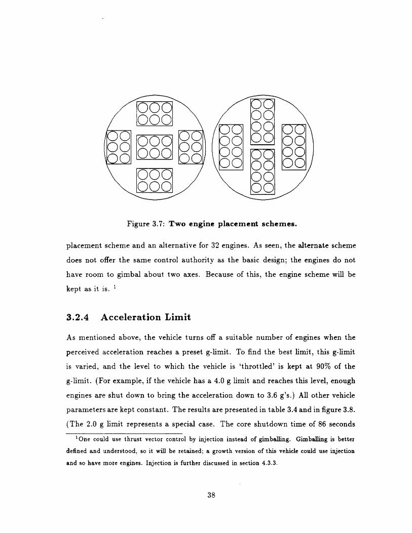
Figure 3.7: Two engine placement schemes.
placement scheme and an alternative for 32 engines. As seen, the alternate scheme
does not offer the same control authority as the basic design; the engines do not
have room to gimbal about two axes. Because of this, the engine scheme will be
kept as it is.
3.2.4 Acceleration Limit
As mentioned above, the vehicle turns off a suitable number of engines when the
perceived acceleration reaches a preset g-limit. To find the best limit, this g-limit
is varied, and the level to which the vehicle is 'throttled' is kept at 90% of the
g-limit. (For example, if the vehicle has a 4.0 g limit and reaches this level, enough
engines are shut down to bring the acceleration down to 3.6 g's.) All other vehicle
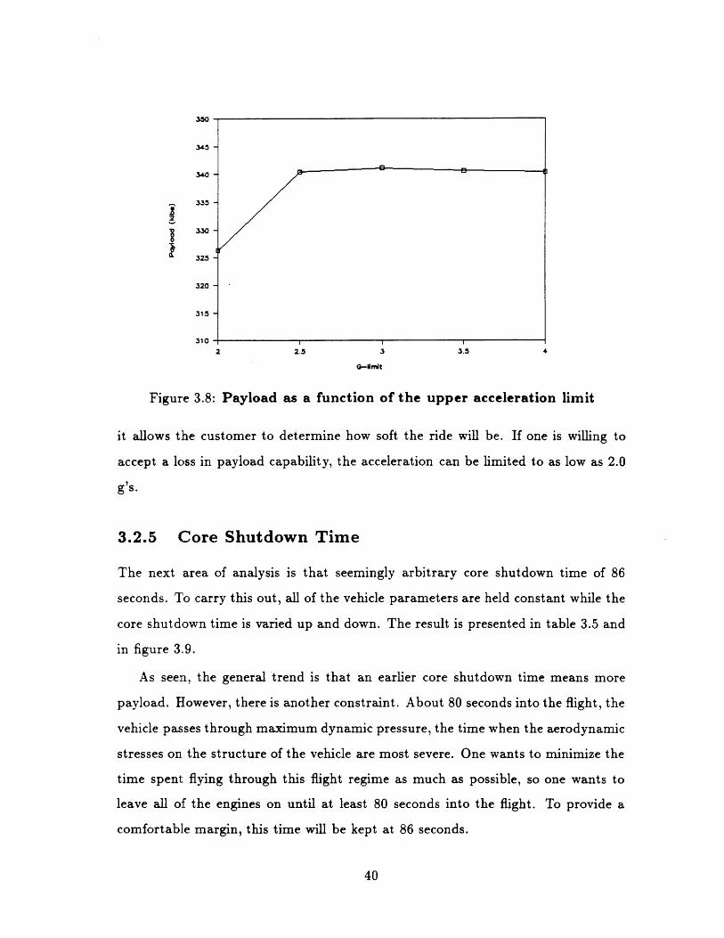
parameters are kept constant. The results are presented in table 3.4 and in figure 3.8.
(The 2.0 g limit represents a special case. The core shutdown time of 86 seconds
'One could use thrust vector control by injection instead of gimballing. Gimballing is better
defined and understood, so it will be retained; a growth version of this vehicle could use injection
and so have more engines. Injection is further discussed in section 4.3.3.
38
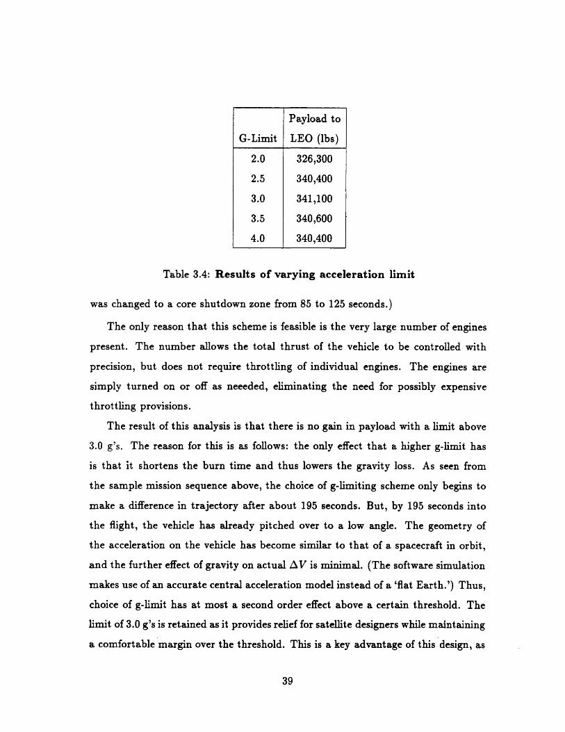
Table 3.4: Results of varying acceleration limit
was changed to a core shutdown zone from 85 to 125 seconds.)
The only reason that this scheme is feasible is the very large number of engines
present. The number allows the total thrust of the vehicle to be controlled with
precision, but does not require throttling of individual engines. The engines are
simply turned on or off as neeeded, eliminating the need for possibly expensive
throttling provisions.
The result of this analysis is that there is no gain in payload with a limit above
3.0 g's. The reason for this is as follows: the only effect that a higher g-limit has
is that it shortens the burn time and thus lowers the gravity loss. As seen from
the sample mission sequence above, the choice of g-limiting scheme only begins to
make a difference in trajectory after about 195 seconds. But, by 195 seconds into
the flight, the vehicle has already pitched over to a low angle. The geometry of
the acceleration on the vehicle has become similar to that of a spacecraft in orbit,
and the further effect of gravity on actual AV is minimal. (The software simulation
makes use of an accurate central acceleration model instead of a 'flat Earth.') Thus,
choice of g-limit has at most a second order effect above a certain threshold. The
limit of 3.0 g's is retained as it provides relief for satellite designers while maintaining
a comfortable margin over the threshold. This is a key advantage of this design, as
39
Payload to
G-Limit LEO (lbs)
2.0 326,300
2.5 340,400
3.0 341,100
3.5 340,600
4.0 340,400
350
345
340
335z
325
325
320
315
3102 2.5 3 3.5 4
-#mit
Figure 3.8: Payload as a function of the upper acceleration limit
it allows the customer to determine how soft the ride will be. If one is willing to
accept a loss in payload capability, the acceleration can be limited to as low as 2.0
g's.
3.2.5 Core Shutdown Time
The next area of analysis is that seemingly arbitrary core shutdown time of 86
seconds. To carry this out, all of the vehicle parameters are held constant while the
core shutdown time is varied up and down. The result is presented in table 3.5 and
in figure 3.9.
As seen, the general trend is that an earlier core shutdown time means more
payload. However, there is another constraint. About 80 seconds into the flight, the
vehicle passes through maximum dynamic pressure, the time when the aerodynamic
stresses on the structure of the vehicle are most severe. One wants to minimize the
time spent flying through this flight regime as much as possible, so one wants to
leave all of the engines on until at least 80 seconds into the flight. To provide a
comfortable margin, this time will be kept at 86 seconds.
40
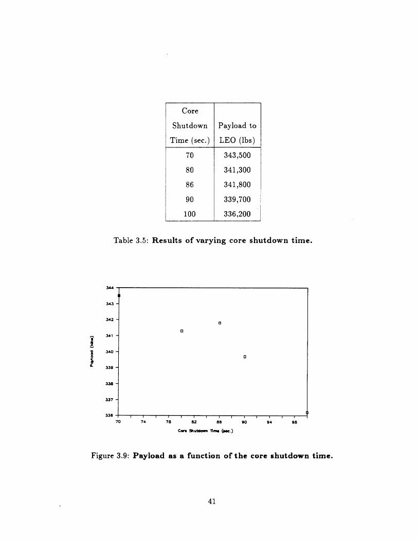
Table 3.5: Results of varying core shutdown time.
43 -
-43
342 -
341
340-
339 -
338 -
337 -
'1It A
70 74 78 82 85
Coa ShutdaMm nim (.)
90 94 98
Figure 3.9: Payload as a function of the core shutdown time.
41
Core
Shutdown Payload to
Time (sec.) LEO (lbs)
70 343,500
80 341,300
86 341,800
90 339,700
100 336,200
3o
To~~~~~~~~
I
lTV I II I I I I
3.2.6 Trade Study Summary
The trade studies above have all maximized the payload capacity within certain
constraints. The fuel loading in the core and strap-on provides for maximum pay-
load delivery, subject to a liftoff weight constraint. The engine placement must
remain the same to provide enough room for gimballing. Acceleration limits have
almost no effect on payload above a certain threshold, and so the previous limit
is retained. The core shutdown time remains the same because of aerodynamic
constraints. The result of this phase of analysis is a vehicle size, engine placement
scheme, and mission sequence that can deliver the maximum payload subject to
several constraints.
3.3 Variation Studies
3.3.1 Mass Fraction
The first parameter that will be varied is the mass fraction. As mentioned in the
derivation, a mass fraction of 0.1 seems reasonable, but after design and construction
this figure could move up or down. For the following analysis, all of the vehicle
parameters are held constant except for the inert stage weights. In other words,
the propellant weights are held constant while the stage weights change, resulting
in a change in mass fraction. The mass fraction of the core and strap-ons are varied
separately.
Core Mass Fraction
Since the core goes to orbit along with the payload, the gain or loss in core mass
is precisely equal and opposite to the loss or gain of payload mass. (This analysis
is the only one which does not use computer simulation for each data point as the
one-to-one relation makes the payload variation a straightforward calculation.) This
42
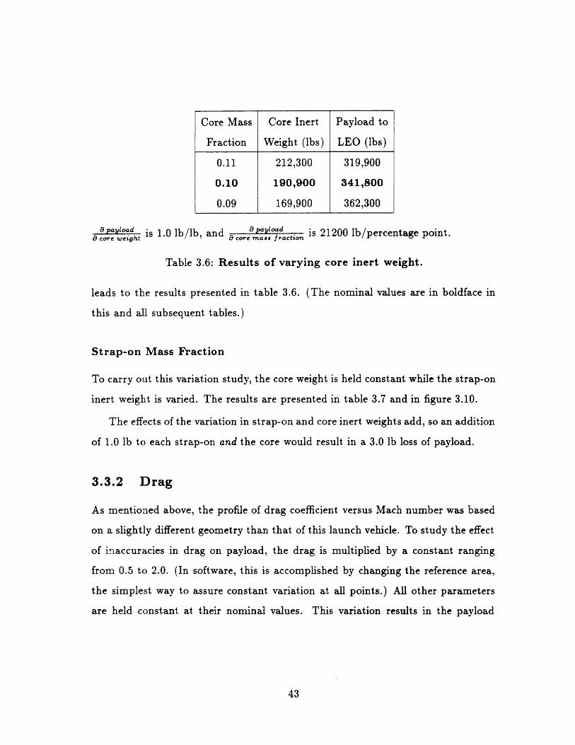
9 ayltoad_ is 1.0 lb/lb a and a factioad is 21200 lb/percentage point.a core weight coa e mass fraction
Table 3.6: Results of varying core inert weight.
leads to the results presented in table 3.6. (The nominal values are in boldface in
this and all subsequent tables.)
Strap-on Mass Fraction
To carry out this variation study, the core weight is held constant while the strap-on
inert weight is varied. The results are presented in table 3.7 and in figure 3.10.
The effects of the variation in strap-on and core inert weights add, so an addition
of 1.0 lb to each strap-on and the core would result in a 3.0 lb loss of payload.
3.3.2 Drag
As mentioned above, the profile of drag coefficient versus Mach number was based
on a slightly different geometry than that of this launch vehicle. To study the effect
of inaccuracies in drag on payload, the drag is multiplied by a constant ranging
from 0.5 to 2.0. (In software, this is accomplished by changing the reference area,
the simplest way to assure constant variation at all points.) All other parameters
are held constant at their nominal values. This variation results in the payload
43
Core Mass Core Inert Payload to
Fraction Weight (lbs) LEO (lbs)
0.11 212,300 319,900
0.10 190,900 341,800
0.09 169,900 362,300
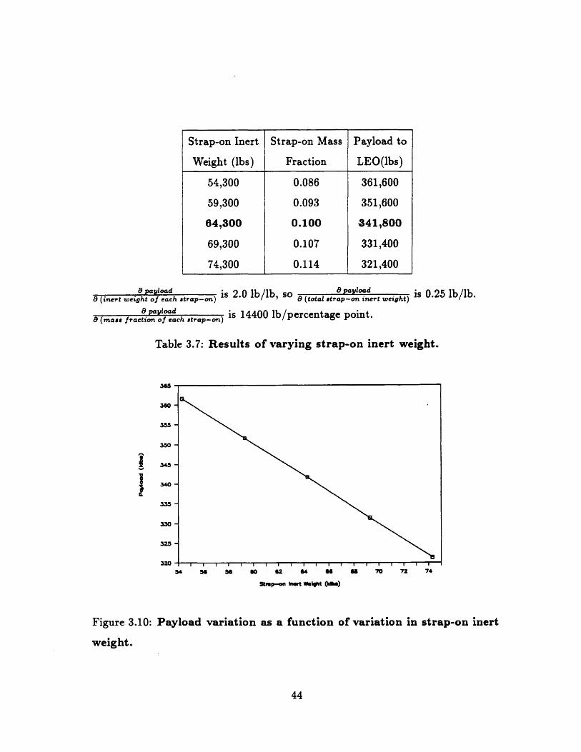
w payload is 2.0 lb/lb, so 8 payloadi 2ba (inert weight of ach trap-on) 0 lb/lb (total strap-on inert weight) is 0.25 lb/lb.8 payload i140bprnta pnt
8 (mass fraction of each atrap-on) is 14400 lb/percentage point.
Table 3.7: Results of varying strap-on inert weight.
365-
355 -
I350 -
345-
340-
335 -
330 -
325 -
320 -54
I I I I I I I TU 1 II I i- I I I I I I I I I I I I !
56 5 o0 62 64 6 6 70 72 74
Stmp--on hwt Wight (i)
Figure 3.10: Payload variation as a function of variation in
weight.
strap-on inert
44
Strap-on Inert Strap-on Mass Payload to
Weight (bs) Fraction LEO(lbs)
54,300 0.086 361,600
59,300 0.093 351,600
64,300 0.100 341,800
69,300 0.107 331,400
74,300 0.114 321,400
_
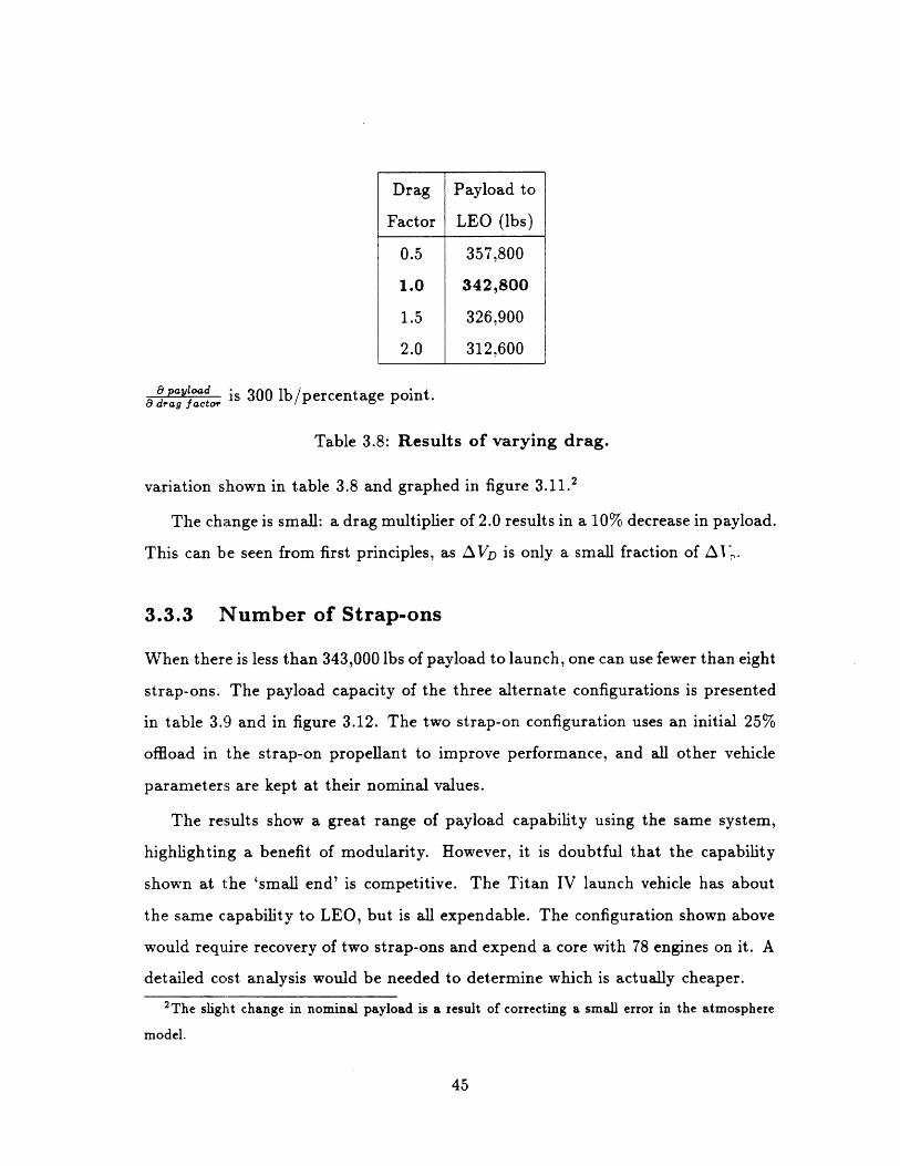
paloadt is 300 lb/percentage point.c9 drag factor
Table 3.8: Results of varying drag.
variation shown in table 3.8 and graphed in figure 3.11.2
The change is small: a drag multiplier of 2.0 results in a 10% decrease in payload.
This can be seen from first principles, as AVD is only a small fraction of Ai[.
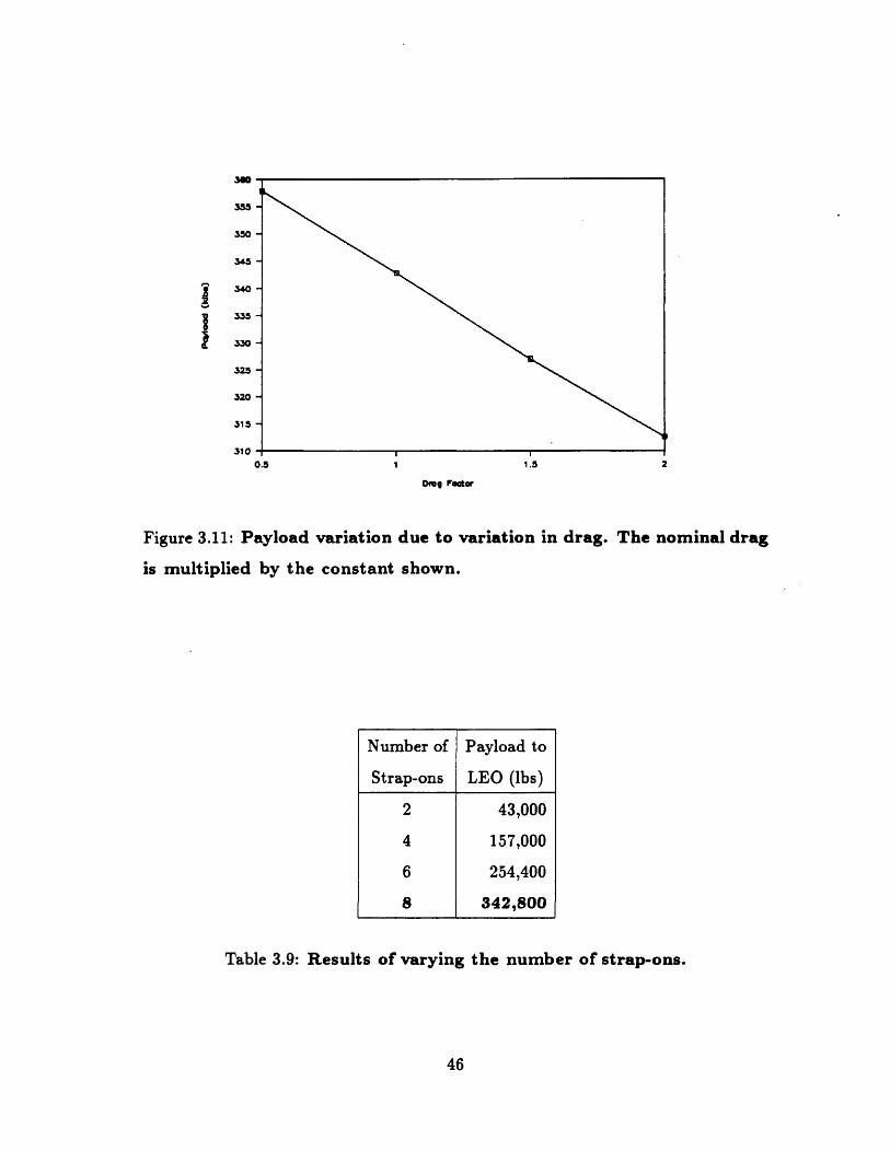
3.3.3 Number of Strap-ons
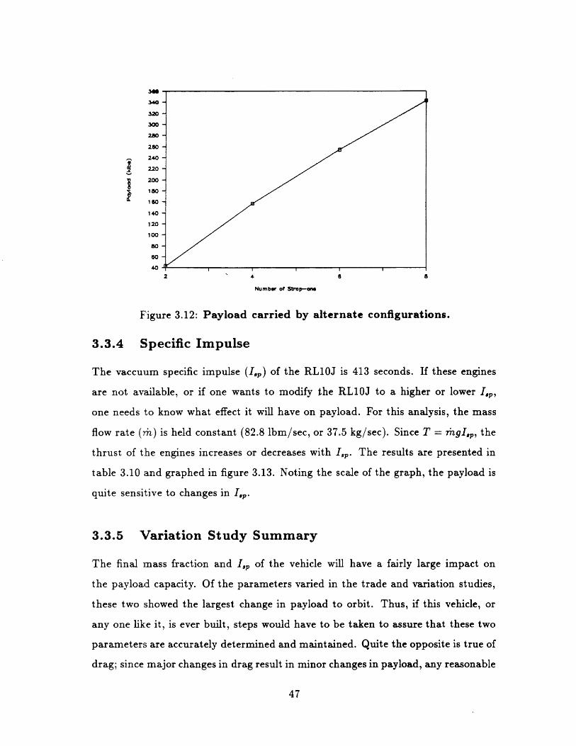
When there is less than 343,000 lbs of payload to launch, one can use fewer than eight
strap-ons. The payload capacity of the three alternate configurations is presented
in table 3.9 and in figure 3.12. The two strap-on configuration uses an initial 25%
offload in the strap-on propellant to improve performance, and all other vehicle
parameters are kept at their nominal values.
The results show a great range of payload capability using the same system,
highlighting a benefit of modularity. However, it is doubtful that the capability
shown at the 'small end' is competitive. The Titan IV launch vehicle has about
the same capability to LEO, but is all expendable. The configuration shown above
would require recovery of two strap-ons and expend a core with 78 engines on it. A
detailed cost analysis would be needed to determine which is actually cheaper.2The slight change in nominal payload is a result of correcting a small error in the atmosphere
model.
45
Drag Payload to
Factor LEO (lbs)
0.5 357,800
1.0 342,800
1.5 326,900
2.0 312,600
I3
355
350
345
340
335
1 330
325
320
315
3100.5 1.5 2
Drg osar
Figure 3.11: Payload variation due to variation in drag. The nominal drag
is multiplied by the constant shown.
Table 3.9: Results of varying the number of strap-ons.
46
Number of Payload to
Strap-ons LEO (lbs)
2 43,000
4 157,000
6 254,400
8 342,800
340
320
300
2ao
280
240
2 220
200
180160
140
120
100
80
402 ' 4 6 8
Number of SUp-mna
Figure 3.12: Payload carried by alternate configurations.
3.3.4 Specific Impulse
The vaccuum specific impulse (Ip) of the RL1OJ is 413 seconds. If these engines
are not available, or if one wants to modify the RL1OJ to a higher or lower Ip,
one needs to know what effect it will have on payload. For this analysis, the mass
flow rate ( ?n) is held constant (82.8 lbm/sec, or 37.5 kg/sec). Since T = mgIp, the
thrust of the engines increases or decreases with I,p. The results are presented in
table 3.10 and graphed in figure 3.13. Noting the scale of the graph, the payload is
quite sensitive to changes in Ip.
3.3.5 Variation Study Summary
The final mass fraction and Ip of the vehicle will have a fairly large impact on
the payload capacity. Of the parameters varied in the trade and variation studies,
these two showed the largest change in payload to orbit. Thus, if this vehicle, or
any one like it, is ever built, steps would have to be taken to assure that these two
parameters are accurately determined and maintained. Quite the opposite is true of
drag; since major changes in drag result in minor changes in payload, any reasonable
47
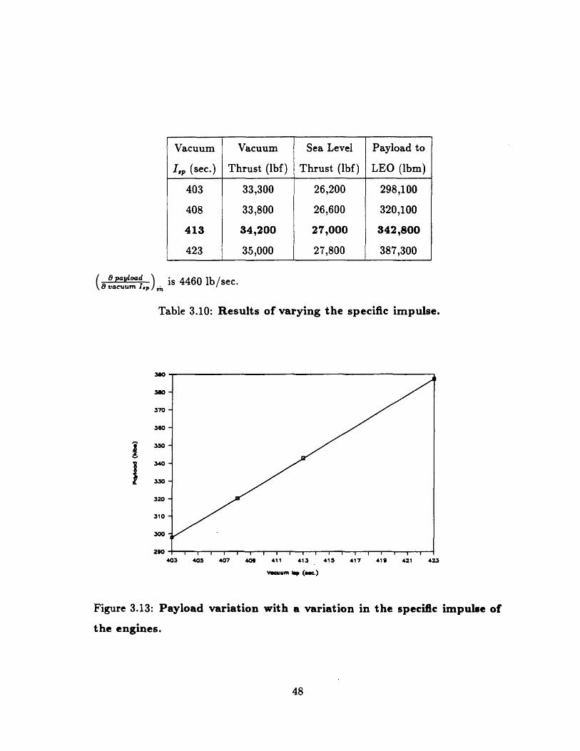
( payoad ) is 4460 lb/sec.Ta ble vacuum impulse.
Table 3.10: Results of varying the specific impulse.
30
3W0
370
380
340
i 330
320
310
300
290403 405 407 409 411 413 415 417 419 421 423
Vaa um %P (e.)
Figure 3.13: Payload
the engines.
variation with a variation in the specific impulse of
48
Vacuum Vacuum Sea Level Payload to
I, (sec.) Thrust (lbf) Thrust (lbf) LEO (bm)
403 33,300 26,200 298,100
408 33,800 26,600 320,100
413 34,200 27,000 342,800
423 35,000 27,800 387,300
estimate of drag should result in a good estimate of payload. The payload carried
by alternate configurations shows the flexibility of this highly modular design.
3.4 Trajectory Description
Below is a series of graphs that depict many key trajectory parameters as functions
of time. Many of these parameters show the same profile as with any launch vehicle,
but some show features unique to this design.
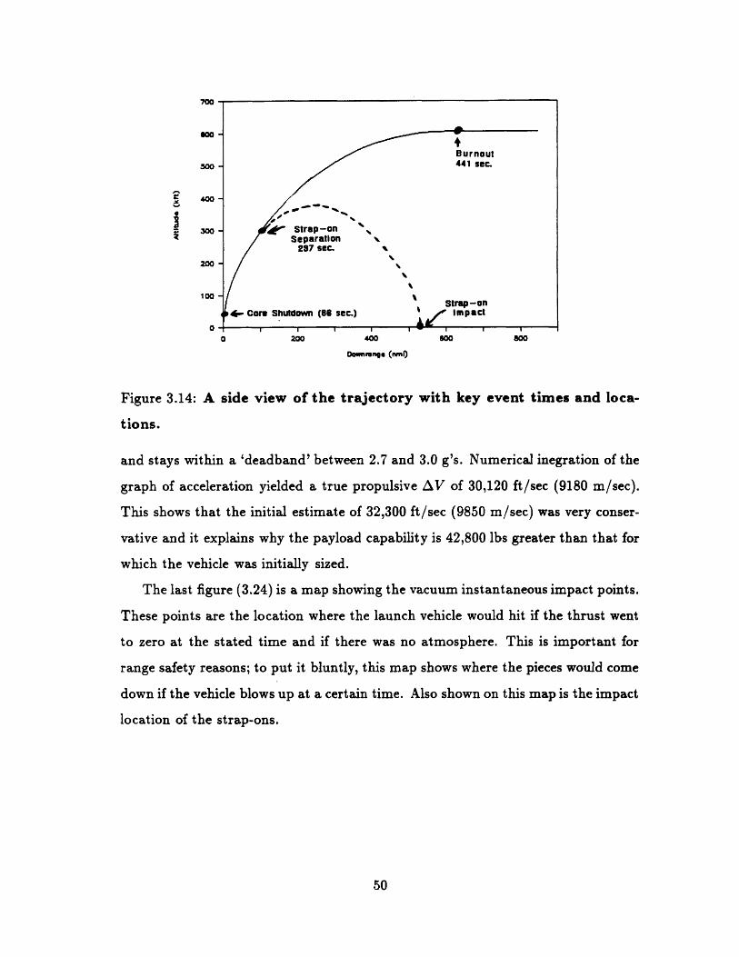
The first graph (figure 3.14) is one of downrange distance versus altitude. This
gives one a physical feel for the shape of the trajectory as well as summarizing the
time and location of major flight events.
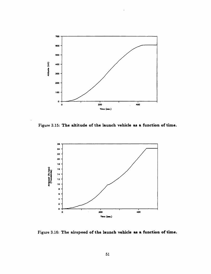
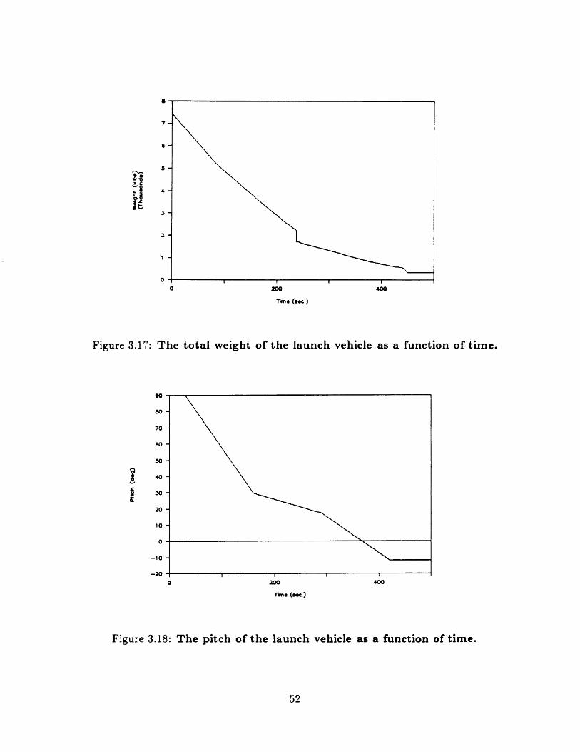
The next three graphs are of altitude, relative velocity (or airspeed), and weight
as functions of time (figures 3.15 through 3.17). All of these graphs are not all that
different from existing launch vehicles. The dramatic effects are primarily due to
mission sequence events; for example, the staging of the strap-ons show as a bend
in the graph of weight versus time.
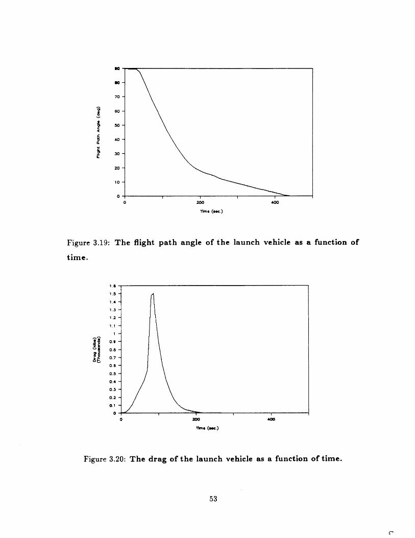
The next two graphs (figures 3.18 and 3.19) show the pitch and flight path
angle as functions of time respectively. Pitch is defined as the angle between the
thrust vector and the local horizontal, while flight path angle is defined as the angle
between the velocity vector and the local horizontal. The pitch is less than zero
at burnout because the vehicle must thrust downward in order to circularize. The
graph shows the effect of the simplified guidance scheme discussed in section 3.1.1.
The flight path angle reaches zero at burnout as the vehicle is going into a circular
orbit.
The next two graphs (figures 3.20 and 3.21) show drag and dynamic pressure
as respective functions of time. Both have a sharp peak as in the example used to
estimate AVD in advance (figure 2.2). The graphs of thrust and perceived accelera-
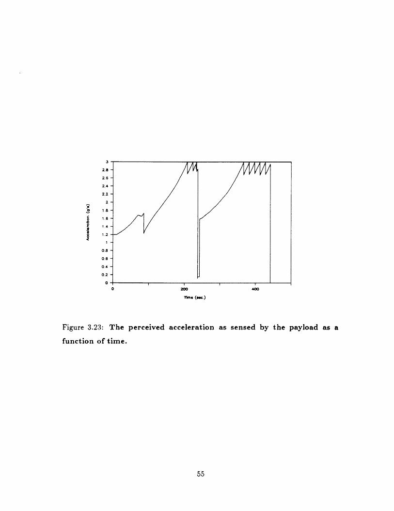
tion (figures 3.22 and 3.23) show the result of g-limitation. The acceleration reaches
49
700
00
500
400
300
200
100
lo
0 200 400 600 800
Domwnrnge (m)
Figure 3.14: A side view of the trajectory with key event times and loca-
tions.
and stays within a 'deadband' between 2.7 and 3.0 g's. Numerical inegration of the
graph of acceleration yielded a true propulsive AV of 30,120 ft/sec (9180 m/sec).
This shows that the initial estimate of 32,300 ft/sec (9850 m/sec) was very conser-
vative and it explains why the payload capability is 42,800 lbs greater than that for
which the vehicle was initially sized.
The last figure (3.24) is a map showing the vacuum instantaneous impact points.
These points are the location where the launch vehicle would hit if the thrust went
to zero at the stated time and if there was no atmosphere. This is important for
range safety reasons; to put it bluntly, this map shows where the pieces would come
down if the vehicle blows up at a certain time. Also shown on this map is the impact
location of the strap-ons.
50
700
o0
540
C 400
300
200
100
00 200 400
Time (ec.)
Figure 3.15: The altitude of the launch vehicle as a function of time.
2
24
22
20
18
16
1 14
2
00 200oo 400
ime (me.)
Figure 3.16: The airspeed of the launch vehicle as a function of time.
51
___
.
7
ze
:2 x i0-2'I
5
4
3
o
00 200 400
Tm. (eec.)
Figure 3.17: The total weight of the launch vehicle as a function of time.
9o80
70
60
50
I41K
40
30
20
10
0
-10
-200 200 400
Time (ee.)
Figure 3.18: The pitch of the launch vehicle as a function of time.
52
90
7070
II
r,
80
50
40
30
20
10
00 200 400
Time (c.)
Figure 3.19: The flight path angle of the launch vehicle as a function of
time.
1.5
1.5
1.4
1.3
1.2
1.1
1' o.g
a 0.8
0.8
0.5
0.40.3
0.2
0.1
00 200 400
Time ("c.)
Figure 3.20: The drag of the launch vehicle as a function of time.
53
C-
GM0
500
Ii
IAQ
E
IIL2EI
400
300
200
100
00 200 400
ome (ec.)
Figure 3.21: The dynamic pressure on the launch vehicle as a function of
time.
11
10
9
a
7
1 '
4
3
2
1
00 200 400
Tkme (.)
Figure 3.22: The thrust of the launch vehicle as a function of time.
54
2.8
2.6
2.4
2.2
2.
1.8
o 1.8
i .4
1 1.2
0.8
0.6
0.4
0.2
00 200 400
Time (c.)
Figure 3.23: The perceived acceleration as sensed by the payload as a
function of time.
55
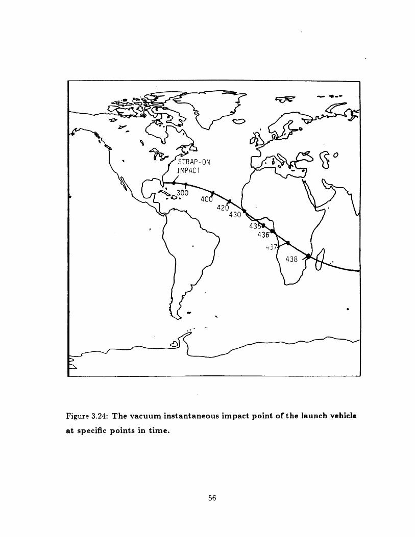
Figure 3.24: The vacuum instantaneous impact point of the launch vehicle
at specific points in time.
56
Chapter 4
Engine Failure
4.1 Overview
Of the failure modes of a launch vehicle, the one that seems the most likely to occur
on this vehicle is having an engine fail in flight. With 30 engines per strap-on, there
will probably not be time to inspect every engine after each flight. When combined
with the core engines, which presumably will have previously been flown on strap-
ons, there are 318 engines, most of which have been used and few of which have
been closely inspected since leaving the factory. Although these engines are simple
enough to permit extensive qualification testing, the fact that there are 318 of them
means that the possibility of an engine failing is higher than that of other launch
vehicles. Further, since one is carrying 340,000 pounds of expensive payload, one
must take steps to insure that an engine failure will not jeopardize the mission.
If an engine failure is fracticidal (that is, if the engine fails by exploding), then the
launch vehicle will almost certainly be destroyed. The force of an engine explosion
will rupture much of the rest of the vehicle. Fortunately, it is difficult for the
RL10J to fail this way. Its simple design draws less and less propellant in the
event of malfunction, virtually guaranteeing a safe shutdown. Further, the engine
operates with comparatively low chamber pressure, guarding against some kind of
57
structural failure. For example, the RL10J operates at a pressure of 575 psi (3960
kPa) [2] where the Space Shuttle Main Engine operates at nearly 3000 psi (20,600
kPa) [1, page A-53].
If an engine failure is fratricidal (that is, if one engine failure causes the whole
cluster to fail), then having a cluster, or clusters, out must be considered. Without
examining plumbing and other possible failure modes, this type of failure seems
more likely and more survivable than the fracticidal failure. Thus, this 'cluster out'
will be investigated as well as a single engine out.
The first issue associated with engine failure is that of performance. Clearly,
fewer working engines means less payload, but the question is how fast this perfor-
mance falls off. The second issue is that of control authority. Having an engine out
means asymmetric thrust, and this must somehow be corrected. Before calculating
the control needed for correcting failed engines, one needs to calculate the control
for the nominal case. The third issue is that of propellant management. When
an engine fails on a strap-on, that strap-on will consume propellant more slowly,
resulting in a longer burntime and uneven weight distribution. Each of these issues
is addressed in a separate section below, along with a summary of conclusions.
4.2 Payload Capability
The payload capability of the vehicle with failed engines is dependent on the number
and location of these engines. As can be seen in section 3.2.3 above, one would prefer
to have as many engines on the strap-on as possible, so failed strap-on engines will
have a more negative effect than failed core engines. Further, a failed engine early in
the flight will have a more negative effect than a failed engine later in the flight. To
carry out this analysis, a certain number of core and strap-on engines were assumed
to be non-existent, equivalent to assuming that they had failed from launch and
never work. The results are printed in the table below where, as above, LEO is an
58
350
340
330
320
i 310
300
290
2800 2 4 6 8 10
Percentage of Engines Out
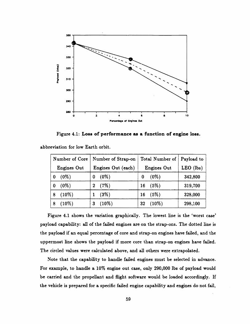
Figure 4.1: Loss of performance as a function of engine loss.
abbreviation for low Earth orbit.
Number of Core Number of Strap-on Total Number of Payload to
Engines Out Engines Out (each) Engines Out LEO (lbs)
0 (0%) 0 (0%) 0 (0%) 342,800
0 (0%) 2 (7%) 16 (5%) 319,700
8 (10%) 1 (3%) 16 (5%) 328,000
8 (10%) 3 (10%) 32 (10%) 298,100
Figure 4.1 shows the variation graphically. The lowest line is the 'worst case'
payload capability: all of the failed engines are on the strap-ons. The dotted line is
the payload if an equal percentage of core and strap-on engines have failed, and the
uppermost line shows the payload if more core than strap-on engines have failed.
The circled values were calculated above, and all others were extrapolated.
Note that the capability to handle failed engines must be selected in advance.
For example, to handle a 10% engine out case, only 290,000 lbs of payload would
be carried and the propellant and flight software would be loaded accordingly. If
the vehicle is prepared for a specific failed engine capability and engines do not fail,
59
Thguit
V.IocIEV
Figure 4.2: The geometry of the thrust, velocity, and drag vectors.
the vehicle can turn off engines deliberately, fly a non-optimal trajectory, cut off
engines before all of the propellant is expended, or perform some combination of
these strategies. This means that the customer can select the reliability of the launch
vehicle in advance, as a higher failed engine capability means higher reliability but
lower performance.
4.3 Control
Before calculating the control needed with failed engines, the control neeaed to
handle a normal flight must be calculated.
4.3.1 Nominal Control
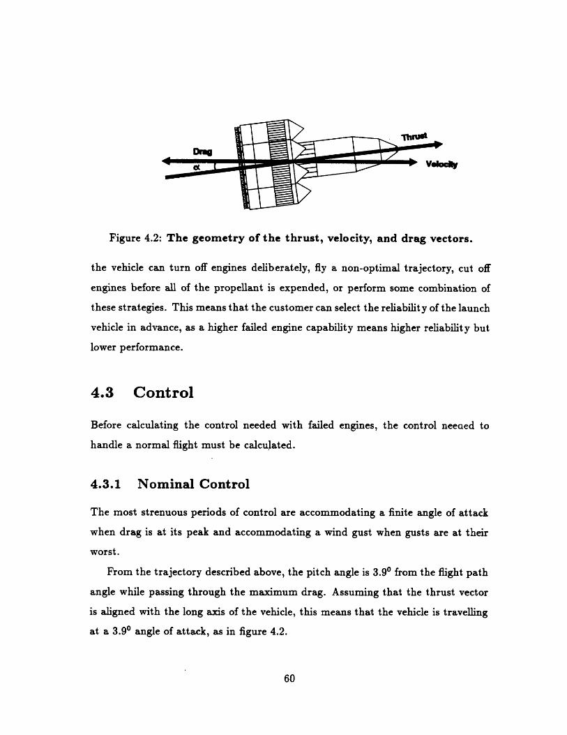
The most strenuous periods of control are accommodating a finite angle of attack
when drag is at its peak and accommodating a wind gust when gusts are at their
worst.
From the trajectory described above, the pitch angle is 3.90 from the flight path
angle while passing through the maximum drag. Assuming that the thrust vector
is aligned with the long axis of the vehicle, this means that the vehicle is travelling
at a 3.90 angle of attack, as in figure 4.2.
60
01 DM
at
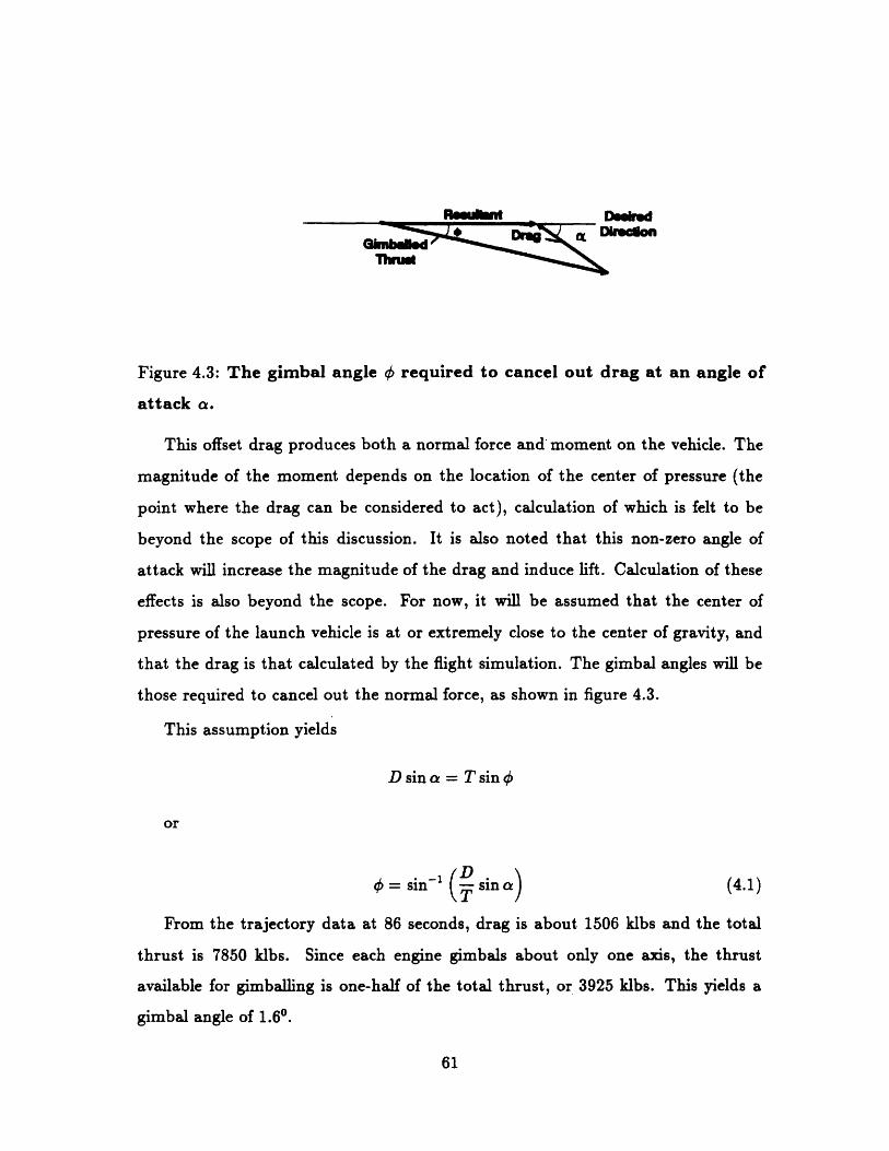
Figure 4.3: The gimbal angle b required to cancel out drag at an angle of
attack a.
This offset drag produces both a normal force and moment on the vehicle. The
magnitude of the moment depends on the location of the center of pressure (the
point where the drag can be considered to act), calculation of which is felt to be
beyond the scope of this discussion. It is also noted that this non-zero angle of
attack will increase the magnitude of the drag and induce lift. Calculation of these
effects is also beyond the scope. For now, it will be assumed that the center of
pressure of the launch vehicle is at or extremely close to the center of gravity, and
that the drag is that calculated by the flight simulation. The gimbal angles will be
those required to cancel out the normal force, as shown in figure 4.3.
This assumption yields
D sin a = T sin o
or
= sin ( sina) (4.1)
From the trajectory data at 86 seconds, drag is about 1506 klbs and the total
thrust is 7850 klbs. Since each engine gimbals about only one axis, the thrust
available for gimballing is one-half of the total thrust, or 3925 klbs. This yields a
gimbal angle of 1.6°.
61
IT EGG
CoalTustafTbnrs
Figure 4.4: Geometry of an engine out and the corrective momeits.
The worst case gust loads occur at 43,000 ft, where the 95 percentile wind with
embedded gust is 270 ft/sec [5, page 19]. The vehicle is already at a 4.20 angle
between the thrust and velocity, and the 270 ft/sec gust on a vehicle travelling at
1350 ft/sec results in a 15.50 total angle between thrust and drag. This number is
excessively high; it must be remembered that this is only an instantaneous angle of
attack but this does show that these gusts will produce severe forces on the launch
vehicle; Using equation 4.1 and the trajectory data at 90 seconds, one obtains a
total gimbal angle of 5.00. Thus, gusts are three times as stringent as simple angle
of attack.
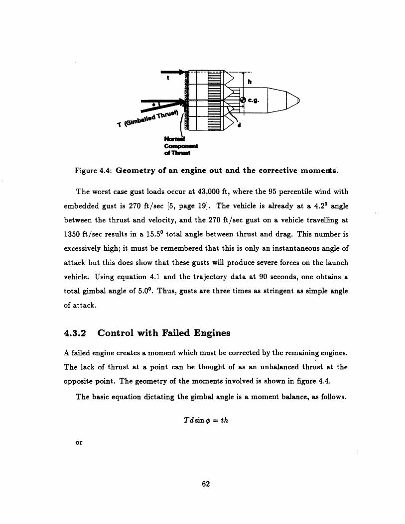
4.3.2 Control with Failed Engines
A failed engine creates a moment which must be corrected by the remaining engines.
The lack of thrust at a point can be thought of as an unbalanced thrust at the
opposite point. The geometry of the moments involved is shown in figure 4.4.
The basic equation dictating the gimbal angle is a moment balance, as follows.
Tdsin = th
or
62
X sin-[(' ) (s)] (4.2)as expressed in dimensionless groupings.
The first item to be calculated is d, the height of the center of gravity. For this
calculation, it was assumed that the weight of each engine is 450 lbs [2], centered
three feet below the base of each core and strap-on. The remainder of the inert
structural weight was assumed to be centered exactly halfway between the base and
the top of each module. The location of the center of gravity was calculated without
any propellant and then with a full load of propellant. It was then assumed that
the location of the center of gravity changed linearly with propellant consumption.
Given all of these assumptions, the center of gravity was calculated to be 49.8 ft
above the base of the core at 90 seconds into the flight. All subsequent calculations
also assume parameter values at 90 seconds into the flight.
Single Engine Out
Assuming an outboard engine has failed, h is the radius of the core plus the diameter
of a strap-on, or 47.2 ft. There are 239 other engines operating, as the core is shut
down. Taking into account single-axis gimballing, there are 239/2 engines available
to correct the 1 engine out. Thus
= sinF' [(j-) (:) 0.50239) 49.8)]
Single Cluster Out
A cluster has a width of 5 ft and is located slightly inboard from the booster edge,
so h is 44 ft. There are 234/2 engines avaible to correct for the 6 engines out. Thus,
= sir' 12 44.0)] 2.60)234 (49.8/
A second cluster out will have less than double the effect, as any other cluster
out will decrease h.
63
Booster Out
Just to study an extreme case, the gimbal angle required to correct for an entire
booster being out will be calculated. The 10% engine out case above has 32 failed
engines, so a booster out can be handled propulsively.
In this case, h is the radius of the core plus the radius of a strap-on, or 34.1 ft.
There are 30 engines out and 210/2 left to steer. This yields
sin-1 [ 1130=in-' [(210 \ 49.8 ] = 11 3°
This, when combined with the gust loads, would be difficult to accommodate.
4.3.3 Control Summary
To handle worst-case gusting and a cluster out on one side, the engines need to gim-
bal eight degrees. This gives a thrust cosine loss of 1%, equivalent to an additional
two engines out in a propulsive sense. Handling a booster out would require sixteen
degrees of gimbal angle, which is felt to be excessive. If more than one cluster
goes out, they need to be far apart from one another if the vehicle is to maintain
control. While one can accommodate up to 5 clusters out propulsively, they cannot
necessarily be accommodated by the control system, so some engineering should go
into preventing fratricidal engine failures.
The two methods that could circumvent the need for gimballing are injection and
control fins. Injection is a method that injects propellant into the nozzle, resulting
in asymmetric thrust. Control fins are vanes located at the base of the launch
vehicle that act as control surfaces, similar to control surfaces on aircraft. Use of
either of these methods could reduce or eliminate the need for gimballing.
64
4.4 Propellant Consumption Management
Another problem with failed engines is that it means that some strap-ons will con-
sume propellant slower than other strap-ons, leading to different burnout times and
accentuating the problem of unequal thrust with unequal weight. Several methods
for correcting this are discussed in a qualitative fashion below.
The most effective and the most complicated method for assuring equal pro-
pellant consumption is to crossfeed propellant between the strap-ons. This will
guarantee simultaneous burnout and will, with the use of controllable valves, allow
one to control the weight of propellant in each strap-on. The disadvantage of this
scheme is that it greatly increases the cost and complexity of an already complicated
propellant feed system, as well as giving the avionics system one more parameter
to control.
A simple way of correcting consumption is to be careful in selecting which engines
are shut down to limit acceleration. In the baseline case, seven engines have been
shut down on each strap-on at the time they burn out. If none of the functioning
engines are shut down on the defective strap-on, and if the only engines that are
shut down are on the working strap-ons, this would allow the defective strap-on to
'catch up' in fuel consumption. The problem with this scheme is that it is time-
limited. Suppose an engine fails at launch. No further engines are shut down until
208 seconds, and burnout occurs at 237 seconds. The 29 seconds of unequal engine
shut down is not enough time to catch up to the 208 seconds of a single failed
engine. This scheme can help other schemes, but it is not enough in itself to correct
the problem.
Another method for changing the thrust as well as the burnout time is to adjust
the engine burn parameters, e.g. the hydrogen/oxygen mixture ratio. This could
either accentuate or alleviate the unequal thrust of the failed engine, as the new
burn parameters will result in a different thrust. By altering the mixture ratio, the
defective strap-on could be made to burn faster and so keep up with the working
65
strap-ons. However, this means more extensive engine testing, hardware, and flight
software and increases the cost and complexity of the engines.
The simplest method of equalizing both thrust and consumption is to shut down
an engine on each strap-on when one fails on a single strap-on. This method is
guaranteed to equalize all of the strap-ons, thus alleviating the need for gimballing.
However, this multiplies the effect of an engine out by a factor of eight.
Overall, then, a strategy employing crossfeeding appears to be too cumbersome
and expensive. This should only be used if it appears that multiple engine failure is
fairly likely. Some combination of the other strategies can be used without drastic
effects on normal performance. For example, a single engine out at liftoff could be
alleviated by turning off one engine on each strap-on just after passing through the
maximum gust zone. As g-limits are encountered, no further engines are turned off
on the defective strap-on until the propellant loading is equalized. The strategies
employed become more complicated with increasingly complex scenarios, as when
engines fail at various points in the flight. Some detailed study would need to be
done in this area, and the results would be incorporated into the flight software.
4.5 Engine Failure Summary
From a propulsive standpoint, engine failure can be accommodated simply by
launching with less than the maximum amount of payload and using a non-optimal
trajectory if no engines fail. From the standpoint of controls, an eight degree engine
gimbal capacity can insure vehicle control during maximum gusts with an outboard
cluster out. Whether the vehicle can handle more engines out depends on where
these engines are located. Use of fins or injection techniques can increase the avail-
able control authority. From a propellant standpoint, the vehicle will have to shut
down or throttle down engines on the fully functioning strap-ons in order to even
out propellant consumption. A shutdown could take part as normal acceleration
66
limitation or as a premature shutdown. The throttling down could be carried out
by varying the propellant ratio.
Engine failure, then, can be credibly handled by gimballing and engine shutdown,
leading one to conclude that an engine failure will not jeopardize the mission.
67
Chapter 5
Conclusion
The goal of this study has been to demonstrate that one does not need to use
complex and expensive rocket engines in order to deliver large amounts of payload
to low Earth orbit. A design using over 300 small engines was derived by using the
rocket equations to determine propellant capacity and using this capacity to size
the propulsion system, strap-on boosters, and propellant tanks.
This initial design, featuring 78 engines placed on a 42 ft diameter core and
eight 26 ft diameter strap-ons with 30 engines apiece, was then refined by vary-
ing five design parameters and selecting values which maximized payload capacity
within constraints. These parameters were liftoff mass, core/strap-on size ratio,
core/strap-on engine ratio, acceleration limit, and core shutdown time, and con-
straints included takeoff thrust/weight ratio, space for the engines to gimbal, and
time of maximum dynamic pressure. The most interesting of these studies was the
variation in acceleration limit. This scheme is made possible by the large number
of engines, allowing one to precisely control the thrust by shutting down engines as
needed. The payload capability is virtually a constant when the limit is over 2.5
g's.
Next, several externally determined vehicle parameters were varied to determine
the effect on payload capacity if these parameters have unexpected or non-ideal
68
values. These parameters included mass fraction, drag, number of strap-ons, and
specific impulse. The payload capacity was strongly dependent on specific impulse
and mass fraction, but weakly dependent on drag. The variation in number of
strap-ons showed that the highly modular eight strap-on approach resulted in a
wide range of payload capability with the same design.
The increased likelihood of engine failure is somewhat alleviated by the inher-
ent reliability and robustness of the engine design. -Nevertheless, analysis showed
that the vehicle can carry a fairly large amount of payload even with 10% of the
engines out from liftoff. Further, an 80 engine gimbal capacity insures control with
one failed cluster of six engines during maximum gusts, and this control authority
can be augmented by other techniques, such as fins. Several methods of propellant
consumption management were discussed that could alleviate the problem of un-
equal propellant consumption when engines have failed. Some combination of these
methods would control consumption with minimal impact on the nominal system.
In summary, the design is based on engine technology that is decades old, but
it can deliver many times the payload of existing launchers. The customer can
select the acceleration limit (as low as 2.0 g's) and the failed engine capacity (as
high as 10% of the engines failed at liftoff), which are two features that no existing
launchers can offer. Further, the same basic design can carry anywhere from 40,000
to 340,000 lbs to low Earth orbit. The result is a very capable, flexible, and reliable
design.
69

Bibliography
[1] Space Systems Engineering Class. Design of a Mized Fleet Transportation Sys-
tem to Low Earth Orbit, Volume 3. Department of Aeronuatics and Astronau-
tics of Massachusetts Institute of Technology, Cambridge, MA. Spring, 1987.
[2] Brown, J. R. RLOJ Propulsion Status Presentation at Hughes ALS Design
Study In-Plant Review. August 13, 1987
[3] Hill, P. G. and Peterson, C. R. Mechanics and Thermodynamics of Propulsion.
Addison-Wesley Publishing Company, Reading, MI. 1970.
[4] Battin, Richard H. An Introduction to the Mathematics and Methods of Astro-
dynamics. C. S. Draper Laboratory, Cambridge, MA. 1986.
[5] Toelle, R. (ed.) Heavy Lift Launch Vehicles for 1995 and Beyond. NASA Tech-
nical Memorandum TM-86520. National Aeronautics and Space Administra-
tion, Washington, D.C. 1985.
[6] Titan III Commercial Launch Services Payload Users Handbook. Martin Ma-
rietta Denver Aerospace, Denver, CO. 1986.
[7] Atlas H and K Vehicle System Mission Planners Guide. General Dynamics
Convair Division, San Diego, CA. 1984.
[8] Ariane 4 User's Manual. Arianespace, Evry, France. 1983
[9] Fliigge, W. Stresses in Shells. Springer-Verlag, Berlin, Germany. 1962.
70