Analysis of a Spatio-Temporal Clustering Algorithm for ... · Analysis of a Spatio-Temporal Clustering Algorithm for Counting People in a Meeting ... for mixture models and K-Means

Analysis of a Spatio-Temporal ClusteringAlgorithm for Counting People in a

Meeting

Yongjun Jeon, Paul Rybski

CMU-RI-TR-06-04

January 2006

School of Computer ScienceCarnegie Mellon University

Pittsburgh, Pennsylvania 15213

c© Carnegie Mellon University

Abstract

This paper proposes an algorithm that, given a time intervaland the positions of peo-ple’s faces located by a face detector, automatically determines the number of peoplepresent at a meeting. It should be noted that such a face detector often times producesnoise and false positives, rendering the analysis of its results increasingly difficult. Inany given frame, false positives may appear, and legitimatefaces can go unnoticed,which calls for the use of statistical methods in the algorithm.

Exploiting clustering patterns based on temporal and spatial alignments of the de-tected faces, our algorithm employs the expectation-maximization (EM) algorithm [4]for mixture models and K-Means clustering algorithm [8]. The Gaussian mixturemodel [2] is used to estimate the probability density function of the data points; itsparameters are then optimized using the EM algorithm, whoseperformance is in turnenhanced by its joint use with the K-Means algorithm. Also, by performing randomrestarts in the final model verification stage of the algorithm, different estimates aresampled using different parameters, and the most consistent result is chosen, under theassumption that an incorrect parameter set will have inconsistent fitting.

The results from this combination of algorithms and the sample training data setindicate the existence of the optimal set of parameters thatproduces estimates withlocally minimum standard deviation and percentage error.

Finally, a stand-alone module will first be trained with a data set for which theground truth is available for calculation of percentage errors. It will also implement anautomatic, but simplified, model verification procedure with the parameters obtainedfrom the data set.

I

Contents

I Introduction 1

II Related Work 1

III Approach 2

1 Visual Reconstruction of Data Points 2

2 Mixture Model 3

3 Expectation-Maximization (EM) Algorithm 5

4 EM Algorithm for Gaussian Mixture Model 6

5 K-Means Clustering Algorithm 8

6 Model Verification 86.1 Initial Approach . . . . . . . . . . . . . . . . . . . . . . . . . . . . . 96.2 Devising an Improved Method for Model Verification . . . . .. . . . 10

6.2.1 Evaluation of K-Means Partitioning by Initial EM Likelihood 106.2.2 Controlling the Sampling Rate . . . . . . . . . . . . . . . . . 116.2.3 Dividing the Entire Clip into Subintervals . . . . . . . . .. . 116.2.4 Running a Second EM without Overlapping Points . . . . . .12

7 Putting It All Together 14

IV Results and Findings 14

8 Plain EM Procedure 16

9 EM from K-Means 179.1 K-Means . . . . . . . . . . . . . . . . . . . . . . . . . . . . . . . . 17

9.1.1 Initial K-Means . . . . . . . . . . . . . . . . . . . . . . . . . 179.2 EM . . . . . . . . . . . . . . . . . . . . . . . . . . . . . . . . . . . 189.3 Images . . . . . . . . . . . . . . . . . . . . . . . . . . . . . . . . . . 19

10 Demonstration of Initial Model Verification 19

11 Improved Model Verification 2111.1 Clip 1 . . . . . . . . . . . . . . . . . . . . . . . . . . . . . . . . . . 2311.2 Clip 2 . . . . . . . . . . . . . . . . . . . . . . . . . . . . . . . . . . 2511.3 Clip 3 . . . . . . . . . . . . . . . . . . . . . . . . . . . . . . . . . . 25

III

V Conclusions and Future Works 28

List of Tables

1 Pseudocode for initial model verification . . . . . . . . . . . . . .. . 92 Comparison of Standard Deviation and Initial EM Likelihood Evaluations 113 Pseudocode for improved model verification process . . . . . .. . . 154 Result from Plain EM Procedure . . . . . . . . . . . . . . . . . . . . 165 Initial Results of K-Means Algorithm . . . . . . . . . . . . . . . . . 176 Mean points rearranged . . . . . . . . . . . . . . . . . . . . . . . . . 187 Results: EM from K-Means . . . . . . . . . . . . . . . . . . . . . . . 188 Final Results . . . . . . . . . . . . . . . . . . . . . . . . . . . . . . 219 Sample output of a model verification case (Case 5) . . . . . . . .. . 2110 Result: Clip 1 . . . . . . . . . . . . . . . . . . . . . . . . . . . . . . 2411 Result: Clip 2 . . . . . . . . . . . . . . . . . . . . . . . . . . . . . . 2612 Result: Clip 3 . . . . . . . . . . . . . . . . . . . . . . . . . . . . . . 27

List of Figures

1 X-Histogram . . . . . . . . . . . . . . . . . . . . . . . . . . . . . . 22 Y-Histogram . . . . . . . . . . . . . . . . . . . . . . . . . . . . . . . 33 2D Plot . . . . . . . . . . . . . . . . . . . . . . . . . . . . . . . . . 34 2D Plot of face positions at different time intervals . . . . .. . . . . 45 Meeting clip used for comparison,5 clusters . . . . . . . . . . . . . . 106 Clip sampled at 15 fps (left); at 1 fps (right) . . . . . . . . . . . .. . 127 Different clip sampled at 15 fps (left); at 1 fps (right) . . .. . . . . . 128 Before and after removal - Likelihood decrease . . . . . . . . . .. . 139 Before and after removal - EM failure (NaN likelihood) . . . .. . . . 1310 2D Plot of the logfile with all three clusters labelled . . . .. . . . . . 1511 Images of K-Means module, before running (top) and after (bottom) . 1912 Images of EM module, before running (top) and after (bottom) . . . . 2013 A Graphical Illustration of (2): # People vs. Likelihood .. . . . . . . 2214 Screenshots: Clip 1, 03m 47s, 5 people . . . . . . . . . . . . . . . . .2315 Screenshots: Clip 2, 30m 38s, 5 people . . . . . . . . . . . . . . . . .2316 Screenshots: Clip 3, 49m 40s, 8 people . . . . . . . . . . . . . . . . .2317 Clip 1, 03m 47s,5 faces, 1 fps - Std Dev and Absolute % Error . . . . 2518 Clip 1, 03m 47s,5 faces, 15 fps - Std Dev and Absolute % Error . . . 2519 Clip 2, 30m 38s,5 faces, 1 fps - Std Dev and Absolute % Error . . . . 2820 Clip 2, 30m 38s,5 faces, 15 fps - Std Dev and Absolute % Error . . . 2821 Clip 3, 49m 40s,8 faces, 1 fps - Std Dev and Absolute % Error . . . . 2922 Clip 3, 49m 40s,8 faces, 15 fps - Std Dev and Absolute % Error . . . 2923 Flow of the algorithm . . . . . . . . . . . . . . . . . . . . . . . . . . 30

IV

Part I

IntroductionCAMEO (Camera Assisted Meeting Event Observer) is a hardware and software phys-ical awareness system to record and monitor people’s activities in meetings using aperson-specific facial appearance model (PSFAM) for rapid tracking and identificationof people [5]. While generating a omnidirectional video clipof the meeting at 15 fps,CAMEO tracks human faces by correlating the candidate locations in the current framewith those in the previous frames.

The problem being addressed in this project, however, is to determine the number ofpeople present at a meeting, not to track human faces, which motivates an economicalalternative approach without tracking and person-specificface recognition capabilities.It must be noted, though, that the task is not trivial, takinginto account the imper-fections within any face detection algorithm, which creates false positives. So simplycounting the number of detected faces in each frame does not necessarily accomplishthe task; on the other hand, an overlay of multiple consecutive frames is bound to dis-play a pattern - namely, clusters of points - despite the presence of noise, under theassumption that people are seated and thus stay relatively stationary for the duration ofthe meeting. Then, in order to account for the noise and correlate back to the patternsdisplayed in previous frames, it becomes necessary to employ statistical methods inthe analysis of the data. In particular, statistical methods capable of identifying theclusters and evaluating the goodness of the clustering, such as the K-means cluster-ing algorithm [8] and expectation-maximization (EM) [4] algorithm, are examined. Toillustrate this alternative approach, Schneiderman’s face detection algorithm [9] is ap-plied off-line after CAMEO has recorded the meeting on everysingle frame with nocorrelation between any frames.

Part II

Related WorkThe advantage of the Gaussian mixture model is its ability toaccount for the outliers,whose presence is degrading to the overall quality of the clustering. Rather than in-vestigating outliers as a byproduct of a clustering algorithm, Chiu and Fu [7] articulatethe detection of outliers themselves, even in the case of multiple, overlapping clus-ters. However, their algorithm requires that the user specify the number of intervalsto be partitioned in each dimension beforehand, which makesit unattractive for use innoise filtering in the current project, since its overhead may well be equivalent to theoverhead of the entire model verification procedure.

Elkan and Hamerly [3] discuss several improvements on the k-means and the Gaus-sian expectation-maximization algorithms such as the fuzzy k-means and the k-harmonicmeans algorithms and present a new set of such algorithms that outperform both k-means and the Gaussian expectation-maximization algorithms. Nonetheless, the k-

1

harmonic means algorithm, by definition, receives a parameterp, typically p ≥ 2. Thealgorithm in turn uses it as the exponent in computation of harmonic means, which canbe computationally expensive for largep.

Part III

Approach

1 Visual Reconstruction of Data Points

Once all the points are overlaid and plotted on a 2D grid, different clusters of pointsindicate highly probable positions for different faces in aframe. Then the objective athand becomes locating and counting these clusters.

It is necessary to visually reconstruct the data points in order to first verify the ini-tial assumption on clustering pattern and then determine the types of algorithms to use.Hence, the following three diagrams are constructed:

1. An X-Histogram, with the x-coordinates of the detected faces on the x-axis andthe frequency on the y-axis,

2. An Y-Histogram, with the y-coordinates of the detected faces on the x-axis andthe frequency on the y-axis, and

3. A simple 2D plot of the face positions.

Figure 1: X-Histogram

The overlay of the data points from the entire clip, as shown in 3, does exhibitsome clustering pattern, yet it is also useful to be able to observe changes in clusteringpatterns as the meeting proceeds. The scrollbars enable theuser to specify the timeinterval, or the range of frames, to overlay.

2

Figure 2: Y-Histogram

Figure 3: 2D Plot

2 Mixture Model

With the initial assumption verified, the Gaussian mixture model [2] is then employedto estimate the probability density function of the data points. For the sake of com-pleteness, the algorithm is summarized below.

Probability density estimation is essentially searching the space of parameters tofind the most likely probability density functionp(x) from a set of sample pointsxn, n = 1, · · · , N drawn from an unknown function. A mixture model is a particu-lar form of semi-parametric estimation of probability density, creating a general classof functions with a set of parameters whose size is independent of the size of the dataset.

For instance, consider a model with a probability density function which derivesfrom a linear combination of basis functions and withM , the number of basis func-tions, as a parameter. Hence, the probability density function is expressed as a linear

3

Figure 4: 2D Plot of face positions at different time intervals

combination of basis functions, or component densitiesp(x|j) in this case, as

p(x) =

M∑

j=1

p(j)p(x|j).

wherep(x) describes amixture distribution and the coefficientsp(j) are themixingparameters, or theprior probability that the data points originate from componentj ofthe mixture. Intuitively, the following hold for the mixingparameters:

M∑

j=1

p(j) = 1

0 ≤ p(j) ≤ 1

The component density functionsp(x|j) are likewise normalized:∫

p(x|j)dx = 1

2.2.1 - Gaussian Mixture Models [2]The basis functions are the components of a mixture density model, whose param-

eters must achieve maximum likelihood through optimization. We therefore model thedensity of the input data by a mixture model of the form

p(x) =

M∑

j=1

p(j)φj(x)

where the mixing coefficientsp(j) determine the proportion ofφj(x) included in themixture model andφj(x) are the basis functions.

The parameters of the basis functions can then be computed byre-estimation pro-cedures based the application of the EM algorithm on maximization of the likelihood,which is discussed in the next section.

4

3 Expectation-Maximization (EM) Algorithm

EM is used to find the maximum likelihood estimates of parameters in probabilisticmodels, which depend on unobserved, or missing, latent variables. In particular, EM isan iterative approach to achieving the maximum likelihood of the parameters [2].

EM alternates between the two steps: The expectation step, where the expected val-ues of latent variables are computed, and the maximization step, where the maximumlikelihood of the parameters are computed from the given data and the latent variablesare set to their expectations.

The general description of the algorithm is as follows:

Let y be the observed variables and letz be the latent variables.Let p(y, z|θ) be the joint model of complete data with parametersθ.Let Q(θ|θ′) be the expectation of the parametersθ givenθ′; in other words, the expec-tation with respect to the probability densityp(y|z, θ′) :

Q(θ|θ′) = E[log p(y, z|θ)|z, θ′]

=∑

z

[log p(y, z|θ) · p(z|y, θ′)]

Following the procedure below, the EM will then iterativelyimprove the initial estimateθ0 and construct new estimates:

1. Seti = 0 and chooseθi arbitrarily.

2. ComputeQ(θ|θi).

3. Chooseθi+1 so that it maximizesQ(θ|θi); that is,

θi+1 = arg maxθ

[Q(θ|θi)]

and thenθi+1 is the value maximizing the expectation of complete data log-likelihood with respect to the conditional distribution ofthe latent data.

4. If θi 6= θi+1, then setθi = θi+1 and return to step 2.

It is important to note the following two facts about the EM iteration:

• It can be shown that an EM iteration does not decrease the observed data likeli-hood function; that is,

p(y|θi+1) > p(y|θi)

• The fixed, data-dependent parameters of the functionQ are calculated in the firststep of the procedure. The function is fully determined oncethey are known andis maximized in the maximization step.

5

4 EM Algorithm for Gaussian Mixture Model

It is also important to note that EM is a description of a classof related algorithms andnot a particular algorithm; EM is a skeletal structure for other more specific algorithms.Combining 2 and 3, an application of EM arises in determiningthe parameters of thebasis functions of the Gaussian mixture model, given the number of classes to startwith [2].

Assuming each Gaussian component has a covariance matrix that is a scalar mul-tiple of the identity matrix (no correlation between any pair of different random vari-ables), it has the form

p(x|j) =1

(2πσ2j )d/2

· exp(−||x − µj ||

2σ2j

)

And the negative log-likelihood for the data set is defined asfollows:

E = − lnL = −N∑

n=1

ln p(xn) = −N∑

n=1

ln [M∑

j=1

p(xn|j)p(j)]

Remember that the EM is an iterative procedure; lettingpnew be the probability underthe new parameter values andpold be the probability under the old,

Enew − Eold = −∑

n

lnpnew(xn)

pold(xn)

According to the definition of the mixture distribution given in 2,

∆E = Enew − Eold

= −∑

n

ln

∑j pnew(j)pnew(xn|j)

pold(xn)

= −∑

n

ln [

∑j pnew(j)pnew(xn|j)

pold(xn)

pold(j|xn)

pold(j|xn)]

Jensen’s inequality states that∀λj ≥ 0 such that∑

j λj = 1,

∑

j

λj ln(xj) ≤ ln [∑

j

λjxj ]

Noting in the definition ofE that∑

j pold(j|x) = 1,

∆E = Enew − Eold ≤ −∑

n

∑

j

[pold(j|xn) lnpnew(j)pnew(xn|j)

pold(xn)pold(j|xn)]

LettingQ be the right-hand side of the equation, the upper bound on is

Enew ≤ Eold + Q

6

Recall thatE represents the negative log-likelihood; in order to maximize the likeli-hood,Enew must be minimized, which necessarily follows a decrease inQ. For thesake of simplicity, consider the quantityQ which contains the terms ofQ that do notdepend only on the old parameters.

Q = −∑

n

∑

j

pold(j|xn) ln [pnew(j)pnew(xn|j)]

Since the distributionp of interest is a Gaussian mixture model,

Q = −∑

n

∑

j

pold(j|xn)[ln pnew(j) − d · lnσnewj −

||xn − µnewj ||2

2(σnewj )2

] + const

It now remains to differentiate and minimizeQ with respect to the new parametersµnew

j , (σnewj )2, andp(j)new to get the EM update equations for the mixture model.

Note that in minimizingQ, the method of Lagrange multipliers is used with the con-straint that

∑j pold(j|xn) = 1, leavingQ+λ(

∑j pnew(j)−1) for differentiation with

respect topnew(j), which givesλ = N , the number of data points.

µnewj =

∑n pold(j|xn)xn

∑n pold(j|xn)

(σnewj )2 =

1

d

∑n pold(j|xn)||xn − µnew

j ||2∑pold(j|xn)

pnew(j) =1

N

∑

n

pold(j|xn)

whered is the number of components or variables considered in the model.The actual implementation of 4 implements these update equations for each Gaus-

sian component class. It also includes an additional class following uniform distribu-tion to account for the outlying points that practically do not belong to any of the otherclasses - those having equally low likelihood in all the other classes - thereby reducingthe negative effects of the noise which might otherwise deteriorate the quality of theoutcome.

The implemented EM module is based on the K-Means demonstration applet byAkaho [1]. Although 4 intuitively seems well-suited for theproblem, it soon becomesobvious that random initial distribution of classes often does not lead to an accuratelocalization of the clusters, not to mention the need to speed up the algorithm, whichentails appropriately positioning the classes rather thanjust starting off at random lo-cations. A second algorithm is needed; more specifically, a clustering algorithm whichcan partition data points into different clusters and return the representative points, orthe mean points, to be used in the initialization of the EM classes.

Having specified the desired features of the new algorithm, the algorithm consid-ered next is the K-Means clustering algorithm.

7

5 K-Means Clustering Algorithm

K-Means clustering algorithm [2, 8] is an algorithm for partitioning N data pointsxi; 1 ≤ i ≤ N into K disjoint subsetsSj ; 1 ≤ j ≤ K containingNj data points whileminimizing the sum-of-the-squares errorE:

E =

K∑

j=1

∑

n∈Sj

||xn − µj ||2

whereµj is the mean, or the geometric centroid, of the setSj , which is computed by

µj =1

Nj

∑

n∈Sj

xn

and is updated using∆µj = η · (xn − µj)

whereη is thelearning rate parameter.The implemented K-Means module is based on the K-Means demonstration applet

by Matteucci [6]. Now we are able to compute the mean points, but we still have noinformation about the approximate size of each cluster. In order to appropriately sizethe Gaussian mixture classes, the following values are needed - the variance of the x-coordinate, the variance of the y-coordinate, the covariance of the x- and y-coordinates,and the standard deviations of the x- and the y-coordinates of the data points in eachcluster - which calls for the computation of a2 × 2 covariance matrix (of x- and y-coordinates) in the K-Means module.

After the module has computed the mean points and the approximate size of eachcluster, the information is retrieved and passed to the EM module in order to positionand size the Gaussian mixture classes accordingly. The results are satisfactory; theproper positioning and sizing of the classes improves both the accuracy and the run-time significantly. It would be useful to color each point according to the cluster itbelongs to. The implementation of this feature is relatively trivial, partly because it ispartly a feature of the original K-Means module, and no further computation is neededto pass the necessary information to the EM module.

6 Model Verification

The objective of this project is to automatically determinethe number of people presentat a meeting. However, up until this point, despite the enhancements made to the K-Means and the EM modules, the user still has to specify the number of mean pointsK before running the K-Means module and re-run the algorithm until the result visu-ally shows an acceptable partitioning of the points. In order to automatize this crucialstep, a proper method for model verification must be devised.The following two termsare hereby explicitly defined to refer to the specific features of the verification proce-dure. The readers may also find it helpful to refer to the flowchart denoting the modelverification process at the end of the paper (Figure 23).

8

For k k-means classesDo i k-means runs with k classesPick the best set of mean points (maximum initial EM likelihood)

n first EM Runs

Take the run with the greatest likelihoodEnd For

Pick the best trial (maximum EM likelihood)

Table 1: Pseudocode for initial model verification

• An nth trial refers to the collection of subroutines performed withn K-meansclasses.

• Each subroutine includes the notion ofruns, or the iterations of the K-Means orEM module.

6.1 Initial Approach

Since, when automatized, the modules will have to run on their own and not neces-sarily report the results back to the user after every singlerun, a character-based userinterface (CUI) was added in addition to the GUI for easier stand-alone, command-lineoperation.

The initial layout for model verification is as follows, and apseudocode implement-ing the layout is presented afterwards:

1. Receive from the user the following:K, the maximum number of classes for theK-Means module to attempt up to;i, the number of K-Means runs; andn, thenumber of EM runs, and the desired EM accuracy.

2. For each run of K-Means, look at the number of points contained in each partitionproduced by K-Means and choose the trial with thelowest standard deviation (inthe number of points in each partition).

Nonetheless, this approach is flawed because the K-Means module does not ac-count for the outlying points, or the noise, like the EM module does with the additionaluniform class, and low standard deviation - or low differences between the numberof points in each partition - do not necessarily correlate toa better partitioning; eventhough it is generally the case that the K-Means algorithm does tend to partition thedata into disjoint sets of approximately equal size, the inherent randomness in the ini-tialization of the mean points in the K-Means module must be taken in to account, notto mention the fact that the final positions of the mean pointsare determined geometri-cally and the sizes of each set may very well be unequal, depending on the initializationthe mean points. Also note that although on a given interval each cluster may containsimilar number of points due to the facts that the same numberof people are present in

9

the interval and that the face detection algorithm works frame-by-frame, the presenceof noise in the face detection algorithm as well as the possibility of occlusion must betaken into account as well.

6.2 Devising an Improved Method for Model Verification

6.2.1 Evaluation of K-Means Partitioning by Initial EM Likel ihood

Successful selection of the most appropriate K-Means partitioning is influential to thefinal answer that the program will produce; the evaluation ofpartitioning must in-corporate the issue of whether the partitioning separates and captures each distinctiveclusters with a high probability, which is precisely the question the Gaussian mixturemodel addresses, and the EM module in fact quantifies this quality as likelihood. Thus,an improved evaluation of K-Means partitioning is obtainedby passing the partition-ing information to the EM module and then retrieving the initial likelihood value thatit computes. To illustrate the improved performance of the initial EM likelihood eval-uation, a meeting clip is processed using both the standard deviation method and theinitial EM likelihood evaluation. Figure 5 shows the orientation of the data points ofthe 5 people’s faces throughout this particular meeting. Table 2 shows the results of the

Figure 5: Meeting clip used for comparison,5 clusters

comparison. The lowest standard deviation value appears inbold in standard deviationcolumn. Likewise, the greatest initial likelihood value appears in bold in initial like-lihood value column. As the table shows, the two boldfaced values do not appear inthe same row. It also shows that, in this particular experiment, the standard deviationmethod actually led to the wrong conclusion by the program.

10

Run Std Dev in Initial EM Correctly Spotted# Points Likelihood All 5 Clusters

1 26544.54 -11.7049049 FALSE

2 26445.77 -11.5552135 TRUE

3 24044.43 -11.6530598 FALSE

4 26444.75 -11.5553968 TRUE

5 34630.97 -11.8339914 FALSE

Table 2: Comparison of Standard Deviation and Initial EM Likelihood Evaluations

6.2.2 Controlling the Sampling Rate

Also crucial to the quality of the final answer is the presenceof noise; a desirable proce-dure would effectively reduce the amount of noise present inthe data while preservingthe unique patterns in the orientation of the points, thereby preserving the clusters aswell. One way to reduce the noise is to reduce the number of samples we take. Underthe assumption that people in a meeting are generally stationary, a small decrease inthe sampling rate does not significantly distort the clusters but reduces the frequencyand the probability of sample noise.

For the purpose of this project, two different sampling rates - 1 fps and 15 fps - areexperimented with.

Figures 6 and 7 illustrates the samples obtained from the same logfile with differentsampling rate; left two and right two are obtained from the same images, respectively.

6.2.3 Dividing the Entire Clip into Subintervals

A question directly following 6.2.2 is whether the clustering pattern is lost when allthe data points are overlaid onto a single frame. It is assumed that people at a meetingremain generally stationary; nonetheless, it is still possible that people move aroundand change seats so as to disturb the clustering pattern in the long run, not to mentionthe cases in which people leave the meeting or new people jointhe meeting. Hence,it makes intuitive sense to examine the whole clip in subintervals; a subinterval isbound to contain less moments of significant movements, or noise, and focusing on asubinterval rather than the entire clip corresponds to examining a smaller set of datapoints, thereby preserving the local characteristic of thedata.

For the purpose of this project, five subintervals of different lengths - 10 seconds,30 seconds, 60 seconds, 100 seconds and the entire clip - are experimented with. Itshould be noted that the number of frames each subinterval contains is dependent onthe chosen sampling rate; that is, a 10-second subinterval at 1 fps contains 150 frames,whereas a 10-second subinterval at 15 ftp contains 10 frames.

11

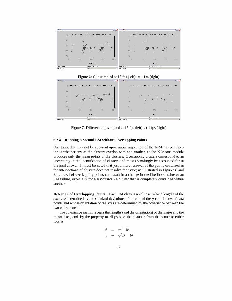
Figure 6: Clip sampled at 15 fps (left); at 1 fps (right)

Figure 7: Different clip sampled at 15 fps (left); at 1 fps (right)

6.2.4 Running a Second EM without Overlapping Points

One thing that may not be apparent upon initial inspection ofthe K-Means partition-ing is whether any of the clusters overlap with one another, as the K-Means moduleproduces only the mean points of the clusters. Overlapping clusters correspond to anuncertainty in the identification of clusters and must accordingly be accounted for inthe final answer. It must be noted that just a mere removal of the points contained inthe intersections of clusters does not resolve the issue; asillustrated in Figures 8 and9, removal of overlapping points can result in a change in thelikelihood value or anEM failure, especially for asubcluster - a cluster that is completely contained withinanother.

Detection of Overlapping Points Each EM class is an ellipse, whose lengths of theaxes are determined by the standard deviations of thex- and they-coordinates of datapoints and whose orientation of the axes are determined by the covariance between thetwo coordinates.

The covariance matrix reveals the lengths (and the orientation) of the major and theminor axes, and, by the property of ellipses,c, the distance from the center to eitherfoci, is

c2 = a2 − b2

c =√

a2 − b2

12

Figure 8: Before and after removal - Likelihood decrease

,

Figure 9: Before and after removal - EM failure (NaN likelihood)

where2a and2b are the lengths of the major and the minor axes, respectively. Further,it is possible to completely determine the locations of focias well as the lengths ofmajor and minor axes, and any point such that

(Sum of distances from the foci) ≤ (Length of major axis)

falls within the boundary of the ellipse or the class, in thiscase. The overlapping pointscan then be detected by keeping track of the number of classesthat each point belongsto.

Weight Function In order to appropriately process the effect of the removal of over-lapping points (since the removal of overlapping points does not always entail an in-crease in likelihood), the relative significance of the effect of the removal is quantified

13

by defining a weight functionp(i). Let Nmax be the maximum number of overlappingpoints in an arbitrary trial, and letNi be the number of overlapping points fromith EMrun. Thenp(i) is defined as follows:

p(i) =

{Ni

Nmax: Nmax > 0

0 : otherwise

Note again that, ifNi = 0, thenp(i) = 0, and ifNi = Nmax, thenp(i) = 1. Based onp(i), a new likelihood valueLnew is computed by mixing the likelihoods prior to (L1)and after (L2) the removal using the following equation:

Lnew = (1 − p(i)) · L1 + p(i) · L2

Note that, ifp(i) = 0, thenLnew = L1, and ifp(i) = 1, thenLnew = L2.

Eliminating a Fixed Upper Bound for the K-Means Module As the number ofK-Means classes increases, either an EM failure is more likely to occur, since eachclass is assigned less points, which degrades the performance of the inherently statisti-cal algorithm, or the occurrence of overlapping points in forms of subcluster becomesmore probable. A pre-set arbitrary constantf determines the maximum number of EMfailure allowed in a trial; that is, a trial will stop upon confronting thenth EM failure.For the purpose of this project,f has been experimentally determined to be 3.

7 Putting It All Together

The following pseudocode in Table 3 implements the improvedmodel verification pro-cedure, which is also illustrated in the flowchart at the end of the paper (Figure 23):

Part IV

Results and FindingsThe logfile used in the first two parts of this experiment (detected faces.txt, 2,197,222bytes) has been prepared by Dr. Paul Rybski. Figure 10 is a 2D plot of all faces in thelogfile.

As it appears in Figure 10, there are three readily identifiable clusters, with a consid-erable amount of noise present in the data set. We label the three clustersA, B andC,respectively, from the left.

To illustrate the improvements made on the performance of the EM module by ini-tializing the EM classes to the mean points returned by K-Means module - which shall

14

For each time intervalFork k-means classes

Do i k-means runs with k classesPick the best set of mean points (maximum initial EM likelihood)

n first EM RunsDetect and remove overlapping pointsn second EM Runs

Determine the two maximum EM likelihoods from the firstand the second EM runs, respectively

Compare and process the max likelihood values of the two usingthe formula and the weight function

The final EM likelihood is then determined for this trialEnd For

Pick the best trial (maximum final EM likelihood)End For

Table 3: Pseudocode for improved model verification process

Figure 10: 2D Plot of the logfile with all three clusters labelled

15

Run # EM # EM Correctly spotted MeanResets Iterations clusters likelihood

1 0 70 A ONLY -9.763452 0 77 A ONLY -9.763443 0 76 A ONLY -9.763444 0 64 A ONLY -9.763455 1 65 A ONLY -9.763456 0 25 C ONLY -10.390177 0 87 A ONLY -9.763448 0 71 A ONLY -9.763459 0 67 A ONLY -9.7634510 0 70 A ONLY -9.76345

Average .1 67.2 - -9.82612Std Dev .3 15.5 - .18802

Table 4: Result from Plain EM Procedure

now be called theEM from K-Means procedure - a comparison of the performances ofthe two procedures is presented: Theplain EM procedure using only the EM algorithmand theEM from K-Means procedure. Also, the desired accuracy of the EM modulein both procedures is empirically set to1.0 × 10−5 and the number of classes to 3, theground truth.

The EM module is designed to be robust, implying that it wouldreset upon encoun-tering an invalid likelihood value such as infinity or NaN. The termEM Resets used inthe tables below refers to this behavior of the program.

Theplain EM procedure is examined first.

8 Plain EM Procedure

As it appears in Table 4, the plane EM procedure spots clusterA correctly with prob-ability Pr[{A}] = 9

10= .9, and the standard deviation of the likelihood values is.188,

which is very large compared to the desired accuracy1.0 × 10−5 specified. In the 10runs conducted, it never spots all three clusters simultaneously. Also, the number ofEM iterations fluctuates greatly at the average of about 67 iterations with the standarddeviation of15.5; the EM module, as per the definition of the EM algorithm, usesrandom initialization of classes, and it is clear from the experimental data that the be-havior of the EM module, indicated by the number of iterations, depends heavily onthe initialization of the classes.

Next, a similar set of experimental data is obtained fromthe EM from K-Meansprocedure and is analyzed. The data from theEM from K-Means procedure is twofold,consisting of the K-Means and the EM portions. To best illustrate the data, three inter-related tables are presented - one table containing the results from the K-Means portionof the procedure, a second one displaying the consistency inthe mean points returnedby the K-Means module, and another table containing the results from the EM portionof the procedure.

16

Run # K-Means # K-Means x1 y1 x2 y2 x3 y3

Resets Iterations1 0 13 782 120 204 152 495 1482 0 15 782 120 204 152 495 1483 0 11 495 148 204 152 784 1204 1 15 495 148 204 152 784 1205 0 9 495 148 204 152 784 1206 2 13 782 120 204 152 495 1487 2 19 204 152 782 120 495 1488 1 15 204 152 495 148 784 1209 1 13 495 148 784 120 204 15210 0 11 204 152 782 120 495 148

Average .7 13.4 - - - - - -Std Dev .8 2.7 - - - - - -

Table 5: Initial Results of K-Means Algorithm

It is important to keep in mind that the K-Means module requires that the user spec-ify the maximumk for the algorithm and that it is the user who determines whether thepartitioning is acceptable upon visual inspection; if it isnot, the user resets the K-Means and runs the algorithm again. The termK-Means resets refers to this action onthe user’s part. Thek is 3 in this case, since there are 3 clusters of interest whosemeanpoints need to be identified. The quantitiesxi, yi ∀i; 1 ≤ i ≤ k respectively refer tothe x- and the y-coordinates of the mean point identified by the ith class.

9 EM from K-Means

9.1 K-Means

9.1.1 Initial K-Means

The K-Means module, on average over the 10 runs, requires approximately 1 man-ual reset, and each run costs about 13 iterations with the standard deviation of2.7.Although not as heavily dependent as the plain EM procedure,the performance of K-Means module, indicated by the number of iterations, does depend on the initializationof the class points, which is also randomly done according tothe definition of the al-gorithm. Moreover, the module produces consistent resultsthat are also correct, giventhat the produced result is visually acceptable; although it may be hard to notice at aglance with the same classes occasionally spotting different clusters, it is clear in Table(6), in which the mean points are rearranged according to theclustersA , B andC, thatthe results are indeed consistent, with 0 as the standard deviations of all the coordinatesexcept that of the x-coordinate of the third class, which is 1.1.

17

Run xA yA xB yB xC yC1 204 152 495 148 782 1202 204 152 495 148 782 1203 204 152 495 148 784 1204 204 152 495 148 784 1205 204 152 495 148 784 1206 204 152 495 148 782 1207 204 152 495 148 782 1208 204 152 495 148 784 1209 204 152 495 148 784 12010 204 152 495 148 782 120

Average 204 152 495 148 783 120Std Dev 0 0 0 0 1.1 0

Table 6: Mean points rearranged

Run # EM # EM Correctly spotted MeanResets Iterations clusters likelihood

1 0 19 A , B, C -9.432082 0 19 A , B, C -9.432083 0 20 A , B, C -9.432084 0 19 A , B, C -9.432085 0 23 A , B, C -9.432076 0 20 A , B, C -9.432087 0 22 A , B, C -9.432078 0 21 A , B, C -9.432079 0 19 A , B, C -9.4320810 0 20 A , B, C -9.43208

Average 0 20.2 - -9.43208Std Dev 0 1.3 - 4.58607 × 10−6

Table 7: Results: EM from K-Means

9.2 EM

The results from the EM module consist Table 7, and the improvements on its perfor-mance, compared to the plain EM procedure, is readily observable. With no resets,the EM module is able to spot all the three clusters of interest with an average of ap-proximately 20 iterations and the standard deviation of 1.3, along with a consistentmean likelihood,−9.43208, whose standard deviation,4.58607 × 10−6, is less thanthe desired accuracy,1.0 × 10−5, whereas the plain EM procedure is unable to spotall the three clusters at once, not to mention the fact that itcosts more iterations andstill produces less precise and less consistent results. Inshort, theEM from K-Meansprocedure produces results that are superior to those of theplain EM procedure withthe only drawback of additional runs of K-Means module.

18

9.3 Images

Figures 11 and 12 are the screenshots of the K-Means and the EMmodules before andafter run, respectively.

Figure 11: Images of K-Means module, before running (top) and after (bottom)

10 Demonstration of Initial Model Verification

The initial verification module described in 6 is called withthe following parameters:

• 10 as the maximumK,

• 10 K-Means runs,

• 1 EM run, and

• 1.0 × 10−5 as the desired EM accuracy.

19

Figure 12: Images of EM module, before running (top) and after (bottom)

10 separate cases of model verification are examined and the results collected,which appear in Table 8.

It is obvious from Table 8 that the method is flawed; it predicts that, on average,there are approximately 9 people, or clusters, when only three are most obvious. Thepresence of a considerable amount of noise contributes to the failure of the method; Ta-ble 9 is the output of model verification run 5, and Table 13 is its graphical illustration,in which it appears that the likelihood values, as a functionof the number of people (orclusters) is an increasing function, although not strictlyincreasing. It seems as thoughthe increased number of classes help the module account for the noise by fitting to thenoise in order to achieve a higher likelihood, for the K-Means module does not accountfor the noise with an additional class like the EM module does.

20

Case Estimated # People Likelihood1 9 -9.075322 10 -9.098583 10 -9.080814 8 -9.121875 9 -9.049306 10 -9.055317 8 -9.059948 9 -9.040779 10 -9.0407610 9 -9.07309

Average 9.2 -Standard Deviation .75 -

% Error -206% -

Table 8: Final Results

...Conclusion===================Likelihood of presence of 1 people : -11.175263033684622Likelihood of presence of 2 people : -10.202015003943165Likelihood of presence of 3 people : -9.713605941990616Likelihood of presence of 4 people : -9.650842812581502Likelihood of presence of 5 people : -9.63814376144801Likelihood of presence of 6 people : -9.236791181913848Likelihood of presence of 7 people : -9.639863491172887Likelihood of presence of 8 people : -9.09046379303053Likelihood of presence of 9 people : -9.049303546534903Likelihood of presence of 10 people : -9.11586615347217

Estimated number of people present: 9

Procedure done. Exiting...

Table 9: Sample output of a model verification case (Case 5)

11 Improved Model Verification

The improved model verification procedure is designed to reduce this fallacy of theinitial model verification method. It is invoked with the following parameters. Notethat the maximumK K-Means classes is not given, since it is now automatically de-termined.

• Unchanged parameters

21

0 2 4 6 8 10−11.5

−11

−10.5

−10

−9.5

−9Sample output of a model verification run

# People

Like

lihoo

d

Figure 13: A Graphical Illustration of (2): # People vs. Likelihood

– 10 K-Means runs,

– 1 EM run, and

– 1.0 × 10−5 as the desired EM accuracy.

• Varied parameters

– Sampling rates: 1 fps, 15 fps

– Interval lengths: 10 seconds, 30 seconds, 60 seconds, 100 seconds, and thewhole clip

5 separate cases of model verification results are obtained for each sampling rateand interval length pair, and the results are collected for the next three new logfiles, fol-lowed by the sample screenshots of each video clip. Note thatthe absolute percentageerror is computed as

|Result − GroundTruth

GroundTruth× 100|

.

• Clip 1, 03m 47s, 5 participants



22

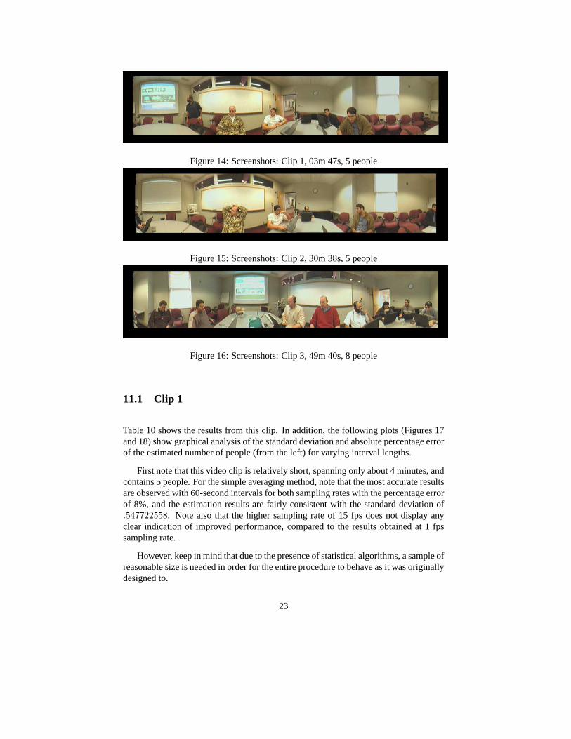
Figure 14: Screenshots: Clip 1, 03m 47s, 5 people



11.1 Clip 1

Table 10 shows the results from this clip. In addition, the following plots (Figures 17and 18) show graphical analysis of the standard deviation and absolute percentage errorof the estimated number of people (from the left) for varyinginterval lengths.

First note that this video clip is relatively short, spanning only about 4 minutes, andcontains 5 people. For the simple averaging method, note that the most accurate resultsare observed with 60-second intervals for both sampling rates with the percentage errorof 8%, and the estimation results are fairly consistent withthe standard deviation of.547722558. Note also that the higher sampling rate of 15 fps does not display anyclear indication of improved performance, compared to the results obtained at 1 fpssampling rate.

However, keep in mind that due to the presence of statisticalalgorithms, a sample ofreasonable size is needed in order for the entire procedure to behave as it was originallydesigned to.

23

Interval Estimated # People Estimated # PeopleLength (sec) at Sampling Rate 1 fps at Sampling Rate 15 fps

(Average) (Average)10 5 410 4 310 4 410 4 410 4 4

Average 4.2 3.8Std Dev 0.447213595 0.447213595% Error -16% -24%

30 7 430 6 430 6 430 7 430 6 4

Average 6.4 4Std Dev 0.547722558 0% Error 28% -20%

60 6 560 5 560 5 660 6 660 5 5

Average 5.4 5.4Std Dev 0.547722558 0.547722558% Error 8% 8%

100 7 6100 4 5100 6 5100 5 6100 6 5


Whole Clip 4 8Whole Clip 2 11Whole Clip 2 8Whole Clip 4 9Whole Clip 4 11

Average 3.2 9.4Std Dev 1.095445115 1.516575089% Error -36% -88%

Table 10: Result: Clip 1

24

Figure 17:Clip 1, 03m 47s,5 faces, 1 fps - Std Dev and Absolute % Error


11.2 Clip 2

The improved verification procedure is performed this time with a larger clip, which is30 minutes long. Table 11 shows the results from this clip. Inaddition, the followingplots (Figures 19 and 20) show graphical analysis of the standard deviation and absolutepercentage error of the estimated number of people (from theleft) for varying intervallengths.

For the simple averaging method, note that the most accurateresults are observedwith 60-second intervals for the sampling rate of 1 fps and with 100-second intervalsfor 15 fps, and both are also the most precise results with thepercentage error of 0%,as it appears in Figures 19 and 20. It is important to remark that now, with a largerset of data, it becomes clear that the absolute percentage error attains a local minimum(which is zero) at interval lengths of 60 and 100 seconds, where the standard deviationalso remains 0. Also notice that, with 1 fps sampling rate, standard deviation becomesgreater than zero and the absolute percentage error obtainsthe local minimum earlier(with respect to the interval length) than it is with 15 fps sampling rate.

11.3 Clip 3

Table 12 shows the results from this clip. In addition, the following plots (Figures 21and 22) show graphical analysis of the standard deviation and absolute percentage errorof the estimated number of people (from the left) for varyinginterval lengths.

Note that, once again, the standard deviation and absolute percentage error both

25


(Average) (Average)10 3 210 3 210 3 210 3 210 3 2

Average 3 2Std Dev 0 0% Error -40% -60%

30 4 330 4 330 4 330 4 330 4 3

Average 4 3Std Dev 0 0% Error -20% -40%

60 5 460 5 460 5 460 5 460 5 4

Average 5 4Std Dev 0 0% Error 0% -20%

100 7 5100 6 5100 6 5100 7 5100 6 5

Average 6.4 5Std Dev 0.547722558 0% Error 28% 0%




26


(Average) (Average)10 6 510 6 510 6 510 6 510 6 5

Average 6 5Std Dev 0 0% Error -25% -37.5%

30 7 630 8 630 7 630 7 630 7 6

Average 7.2 6Std Dev 0.447213595 0% Error -10% -25%

60 8 760 8 760 8 760 8 760 8 7

Average 8 7Std Dev 0 0% Error 0% -12.5%

100 9 7100 8 7100 9 7100 9 7100 8 7

Average 8.6 7Std Dev 0.547722558 0% Error 7.5% -12.5%




27



obtain local minima at the interval length of 60 seconds with1 fps sampling rate; itindeed achieves 0 percentage error and 0 standard deviationsimultaneously with simpleaveraging method. Although the results from 15 fps samplingrate, too, obtain localminima at 60-second interval length, its performance is inferior with -12.5% percentageerror.

Part V

Conclusions and Future WorksWe have thus far described an algorithm to automatically determine the number ofpeople present at a meeting. As an alternative to the face detection approach of thecurrent CAMEO project, the algorithm is a collection of statistical methods such asthe EM and the K-Means algorithms combined together using a model verificationprocedure.

It operates on a set of face positions to estimate the number of distinct, recurringclusters of face positions while taking into account the presence of noise. Given thatthe ground truth for the data set is known (the true number of people present at themeeting is known), it is possible to evaluate the results of the algorithm and find theset of parameters that estimates the number with the lowest standard deviation andpercentage errors.

With the improved model verification method, the algorithm estimates the number

28



of people consistently with reasonable accuracy for a largeset of data points for a givencombination of parameters - 1 fps sampling rate and 60-second interval length in theabove experiment - at which the standard deviation and the percentage error of theestimate attain local minima.

To put it differently, it is possible to obtain the optimal set of parameters to beused in future estimations in the training phase, in which the algorithm operates on thetraining data set for which the ground truth is known, by detecting the local minima ofthe standard deviation and the percentage errors of the estimates.

A stand-alone module for this purpose will implement an automatic, but simplified,training mode for model verification procedure by limiting the search space and adher-ing to 1 fps sampling rate and focusing mainly on the detection of such local minimain the percentage errors.

Ideas have been suggested for further noise filtering via examination of the y-coordinates, based on the observation that there are certain regions of each frame thatare unlikely to contain any face. The exact locations of suchregions are dependent onthe specific orientation of the meeting and the camera. This technique may be imple-mented and experimented using different parameters in the future.

29

Figure 23: Flow of the algorithm

30

References[1] S. Akaho. Em algorithm for mixture models. Internet, 2001.

[2] C. M. Bishop. Neural Networks for Pattern Recognition. Oxford University Press, NewYork, 2004.

[3] C. Elkan and G. Hamerly. Alternatives to the k-means algorithm that find better clusterings.tech. report CS2002-0702, Department of Computer Science and Engineering, University ofCalifornia - San Diego, April 2002.

[4] A. P. Dempster et al. Maximum likelihood from incomplete data via the em algorithm.Journal of the Royal Statistical Society, Series B, 39(1):1–38.

[5] F. De la Torre, C. Vallepsi, P. E. Rybski, M. Veloso, and T. Kanade. Omnidirectional videocapturing, multiple people tracking and identification for meeting monitoring. tech. reportCMU-RI-TR-05-04, Robotics Institute, Carnegie Mellon University, January 2005.

[6] Matteo Matteucci. Clustering - k-means demo. Internet, November 2004.

[7] Anny Lai mei Chiu and Ada Wai chee Fu. Enhancements on local outlier detection. InPro-ceedings of the Seventh International Database Engineering and Applications Symposium.IEEE, 2003.

[8] J. E. Moody and C. J. Darken. Fast learning in networks of locally-tuned processing units.Neural Computation, 1(2):281–294.

[9] H. Schneiderman and T. Kanade. Probabilistic modeling of local appearance and spatialrelationships for object recognition. InIEEE Conf. on Computer Vision and Pattern Recog-nition, pages 45–51. IEEE, 1998.

31

Documents

Analysis of a Spatio-Temporal Clustering Algorithm for ... · Analysis of a Spatio-Temporal Clustering Algorithm for Counting People in a Meeting ... for mixture models and K-Means