Frequency.Response Analysis of Automated Canals

7. A U T H O R I S ) 8. P E R F O S M I N G O R G A N I Z A T I O N REPORT NO. ...

H. T. Falvey - REC-ERC-77-3

9. PERFORMING O R G A N I Z A T I O N N A M E AND ADDRESS 10. HORK UNIT NO.

Engineering and Research Center , .

Bureau of Reclamation Denver, Colorado 80225

13. TYPE O F REPORT AND PERIOD 2 . SPONSORING A G E N C Y N A M E A N 0 ADORE% C O V E R E D

<A;,

Same -r-.>z:.-= I

14. SPONSORI2G A G E N C Y CODE

5. S U P P L E M E N T A R Y NOTES

6. A B S T R A C T

Two methods are available for determining control parameters on automated canals. These are! the transient-response method and the frequency-response method. Since a typical canal system is influenced re dominantly by transient inputs, the transient-response method has been extensively used in the analysis of automated canal systems. The main advantage of the frequency-response method is that the effects of varying :he various control parameterl-can be readily visualized and evaluated. The presently used transient-response nethod and parameter selection are reviewed. The basic concepts of the frequency-rerpons method are ]resented and their application to an automated reach is illustrated with an example. Two computer programs Ire given which can be used to determine canal response characteristics. The state-of-the-art in process control las progressed sufficiently so that both the transient-response and frequency-response methods of analysis can ~e used in a complementary fsshion. Employment of only one method in the design of automated systems is, n general, wasteful of both computer time and, engineering effort.

K E Y WORDS A N 0 DOCUMENT ANALYSIS , , - DESCRIPTORS-- / *automation/ * ranalsl 'analytical techniques1 *frequency analysis1 automatic controll

ntrol equipment1 feedback1 control ivstems

I D E N T I F I E R S - - / Coalinga Canal ."

COSATI F ie ld /Group 09/E COWRR: 0903

DlsTRlsuTlO~ STATEMENT 1 9 . S E C U R I T Y C L I S S 2 1 . NO. OF P A G E

o i lob ie from the Nat ionoi Techn ico i ~n fo rmdt ioo Serv ice, opera t ions ITHIS REPORTI

( i s i o n . Spr ingf ie ld. V i rg in ia 22151. U N C L A S S i F l E D - 69 . , 2 0 . S E C U R I T Y C L A S S 2 2 . PRICE I T H I 5 PAGE)

, UNCLASSIF IED

-- ~ .~

OF AUTOMATED CANALS i -!

..., , ,, . ;; .~. . '..'

,', :# b '*> .

H. T. Falwey

July 1977

H y d r s u l i c s Branch D i v i s i o n o f General R e s e a r c h E n g i n e w i n and R e s e a r c h C e n t e r D e n v e r , C o ? orado

UNITED STATES DEPARTMENT OF THE INTERIOR * BUREAU OF RECLAMATION

ACKNOWLEDGMENT

The analysis desc~ibed in this report has been subjected to a wry careful review by past and present members of the Water Systems Automation Team. Their extremely helpful comments and constructive critmsm is gratefully acknowledged. Mr. D. F. Nelson 1s presently Team Manager.

CONTENTS

Introduction 1 . . . . . . . . . . . . . . . . . . . . . . . . . . . . .

Proportional gain . . . . . . . . . . . . . . . . . . . . . . . . . . 6 Filter time constant 6 . . . . . . . . . . . . . . . . . . . . . . . . . Offset 7 . . . . . . . . . . . . . . . . . . . . . . . . . . . . . .

. . . . . . . . . 8

Fundamental concepts . . . . . . . . . . . . . . . . . . . . . . . . . 8 Reswnse characteristics of control elements . . . . . . . . . . . . . . . . . 12

Basic considerations . . . . . . . . . . . . . . . . . . . . . . . . 12 Filter response . . . . . . . . . . . . . . . . . . . . . . . . . . . 12 Proportifma1 gain response 12 . . . . . . . . . . . . . . . . . . . . . . Reset response 14 . . . . . . . . . . . . . . . . . . . . . . . . . . Combined characteristics of the EL.FLO controller . . . . . . . . . . . . . 14

Response of water level togate movement . . . . . . . . . . . . . . . . . 23 Response characteristics of canals . . . . . . . . . . . . . . . . . . . . 23 Determination of system response functions . . . . . . . . . . . . . . . . 27

Open-loop fesponse 27 . . . . . . . . . . . . . . . . . . . . . . . . Closed-loop response . . . . . . . . . . . . . . . . . . . . . . . 27

System resonance and stability . . . . . . . .

System r e ~ n a n c e 29 . . . . . . . . . . . . . . . . . . . . . . . . . . System stability . . . . . . . . . . . . . . . . . . . . . . . . . 30

Bibliography 32 . . . . . . . . . . . . . . . . . . . . . . . . . . . . Appendix A.-Determination of system frequency-response characteristics

from input and output signals . . . . . . . . . . . . . . . . . . . . . . 35 Appendix B.-Determination of frequency-response characteristics at specific

frequencies by super-imposing asinusoidal signal on the process signal . . . . . . . . 53 Appendix C.-Relationship between wave heights i n a reservoir and wave

heights in a Connecting canal 69 . . . . . . . . . . . . . . . . . . . . . .

TABLES

Response characteristics second reach. Coalinga Canal . . . . . . . . . 27

i

Figure

Closed-loop response second reach, Coalinga Canal . . . . . . . . . . . 29 Srability of closed-loop second reach, Coalinga Canal . . . . . . . . . . 30

FIGURES

Response of a second order r'ystcn to a unit step input . . Schematic representation o i a canal reach . . . . . . . Block diagram of individual canal reach . . . . . . . . Proportional plus reset output from a controller with a

step input . . . . . . . . . . . . . . . ' . . Representation of sinusoidal wave . . . . . . . . . :'. Reduction of nonunity feedback to unity feedback system . Three representations of the frequenw response from Ogata Determination of closed loop response with a Nichols plot . Filter response . . . . . . . . . . . . . . . . Gain response . . . . . . . . . . . . . . . . . Reset response . . . . . . . . . . . . . . . . Response of controller on Coalinga Canal, second resch . . Discharge relationships in a canal reach ' . . . . . . . . Dimensionless frequency parameter . . . . . . . . . Nonlinear control system . . . . . . . . . Inout-outout characteristicsfor an on-off no"i6eariw

with dead band and hysteresis . . . . . . . . . . . . . . .,+. . 20 i.

Frequencv response characteristics on an on-off nonlinearity with dead band and hysteresis . . . . . . . . . . . . . . . . . 21

Dead band stability criteria . . . . . . . . . . . . . . . . . . . 22 Discharge coefficient, radial gate No. 1. Coalinga Canal . . . . . . . . . 24 Frequency response of harbors f rom lppen . . . . . . . . . . . . . 26

. ,., Approximate frequency response, second reach, Coaling2 Canal . . . . . . 27 Open-loop response, second reach, CoalingaCansi . . . . . . . . . . . 28 Closed-loop response, second reach. Coaimga Canal . . . . . . . . . . 29 Stability analysis, second reach, Coalinga Canal . . . . . . . . . . . . 31 Three dimension Bode diagram . . . . . . . . . . - . . . . . . . . 50

INTRODUCTION

The application of automation t o water systems has been well summarized by a "state-of.the-an" report compiled by the USER Water Systems Autxnation Team [I01 ' . Additional details concerning controller equipment have been reported by Buyalski [21. Mz:L&s for determining the parameters for specific controllers have been developed by Shand 191 and Wail [l 11 . These reports all use analysis methods which are derived from control theory; however, the advantages and limi!ations that are inherent with a particular method are not always apparent from the individyal reports. Ogata [71, on the other hand, has very carefully delineated the various analysis methods and their respective areas of applicability. The purpose ,, of this contribution is to put the methods in perspective with respect to water systems automztion and t o i l lus t ra te the applicsbilitv of the frequency-response analysis method.

The main advantap of the frequency-response method is that the absolute and relative stabilities o f a linear, closed-loop system can be determined from the open-loop frequency-response characteristics. Another way of stating this is that the stability of the control system can be determined by knowing the frequency-response characteristics of each part. Since these characteristics can be determined experimentaily, the stability analysis is facilitated. In contrast, the transient-response analysis requires a knowledge of the mathematical expression for the entire system in order .to,i.nystigate the system's stability. For'complicated systems, such as canals, the mathematical expression is almost impossible,to determine. Even with simplifying assumptions. the resulting expression is usually very complicated.

A secondary advantage of the frequency-response method is that the analysis and design can be extended to certain ncnlinear control systems. For instance, the effect of a dead band on a controller can be

more and more s~nusoidal. Therefore, for these cases, the use of the frequency-response method is a The present methods use terms to describe the control reasonable approach. Parameters which are based on the behavior o f a

second order system. The general form of a second ' Numbers in brackets identify referencescontained i n order system can be expressed by the following the bibl~ography. differential equation.

The performance characteristics of a system can be 'investigate3 without the need for trial and error considered as having two components: a transient computer runs. response and a steady-state respcnse. The transient responsc refers to changes that occur i n the output The main disadvantage of the frequency-r?sponse from a system as a resulr of the input passing .from one method i s that for complex systems (higher order state or level t o another state. The steady-state systems i n control systems terminology) the response refers to the oehavior of the output as time becomes infinits: Normally, step, ramp, and impulse inputs are analyzed using transient-response methods: whereas, frequency-response methods are used to analyze sinuaoidal inputs.

The choice of the analysis method to be used is frequently indicated by the expected shape of the signals input into the system. With a single reach of canal, the water demands change by fixed increments. In this case, the typical operation consists of a fixed amount of water being turned out or diverted from the canal. The length of time from the beginning of the 2iversion until the final discharge quantity is reached is so short that the change in discharge can be considered to be a step change. This, in turn. produces a momentary step change in tho water. surface level which actuates the controller. Therefore, the use of the transient-response methods is appropriate.

With multiple reaches of canal, the choice of en analysis method is no longer trivial. As the disturbances Dass further from the site of the turnout, they become

correlation between frequency response and transient response is not direct. For canal systems, this d i f f e r e n c e can be signi f icant since the transient-response characteristics are frequently the most critical with respect to the safety of the structure and the speed with which demands on the system can be met. However, this disadvantage can be overcome; through the use of specific design criteria applied to the frequency-response methods, acceptable transient-response characteristics can be achieved.

In canals, discharge is normally the parameter which i s to be controlled although discharge is not a quantity which can be determined directly. Instead some other quantity must be measured and then discharge is related to that quantity through a mathematical relationship. The quantity most frequently used in canals as the significant parameter i s the water surface elevation or the difference in the water surface elevation between two points. Therefore, in the discussions that follow, the water surface elevation is the controlled parameter.

Shand 191 derived an approximate model for the canal behavior which has the form o f this equation; he ,retained ,ooly the first two terms. i n his derivation, y refel-s t o the change in the downstream water depth. The canal geometry, initial ,,water depths, frictiun factors, etc.. are simulated by different values of the coe f f i c i en t K , . With Shand's simulation, all disturbances decay exponentially.

The addition of a controller (feedback) significantly alters the behavior o f the downstream water surface. Shand I91 showed, for certain control Parameters, a unit step change i n water elevation at the upstream end of t ' e canal produced a damped oscillation, figure 1. with' other zontroi parameters, sustained oscillations will result. The shape o f the tiansient.response curve is essentially determined by five parameters, figure 1. These parameters can be described numerically by either time intervals or amplitudes. The conventional nomenclature which is used t o describe the parameters and the transient-response characteristics. is:

t, = Delay time t, = Rise time tp =Peak time t, = Settling time f,' ,I

M, = Maximum overshot (percenti '.

Ideally, each element of the controller and of the water surface fluctuations in the canal can be described by a mathematical function. These functions and ihe signal flow path through the system can be represented pictorially by a block diagram. For instance, the canal system shown in figure 2 can be represented by the block diagram of figure 3. The capital letter by each block represents a mathematical function which gives

The figure 2 diagram represents downstream control; this i s called downstream control because disturbances are detected downstream of the controlling element. These disturbances are sen:.through a controller :o an ele,neiit which affects the desired remedial action t o eliminate the disturbance. In this case, the controlling element is the upstream gate.

It should be noted at this point that the frequency-response anaiysis methods will work equally well for upstream control. For the purposes o f illustrating the application of frequency-analysis techniques t o canal automation, a $ownstreamcontrol

-3 scheme was selected. ..

the water prism contained between the upstream and dcwstream gates (fig.2). Both upstream and downstream disturbances can effect the water leuzls in the canal reach. This system i s regulated by a controller that attempts t o control the water surface disturbances within certain prescribed limits.

Typical controllers contain filter, proportional, and integral elements. The purposes of the filter are t o compensate for the wave-travel time in the canal reach and t o prevent passage o f ail trivial disturbances from the water level sensor signal. These extraneous d is turbances general ly have high-frequency components and include, among other things, wind waves. The purpose of the proportional element of the controller is t o make the inflow rate through the upstream gate equal t o the d:,tflow rate from the canal resch. To achieve this end, the upstream gate is moved i n proportion t o the change in water level at the sensor. This part o f the controller function i s based upon the assumption that changes in water level at the sensor and changes in the gate position are both directly proportional t o changes in discharge. The purpose of the integral element ia to move the upstream gate in such a fashion that the water level at the sensor i s always returned t o its original position.

The flow o f disturbances through the.system and the controller can he followed on the block diagram, figure 3. In this diagram, G refers t o an element be ing controlled and H refers t o an element on the feedback path. For instance, a turnout at the downstream gate produces t w o signals t h a t travel upstream simultaneously. One. signal passes through the canal itself; the transformation of this signal as i t passes

2

Figure 1 .-Response of a second order ryslem to a untr riep input.

the relationship between signals input into the block and the signals which are output from the block; in other words, the letter represents the transfer function for the block.

UPSTREAM GATE

DOWNSTREAM

through the canal is represented by block G6. The other signal passes through the controller elements Hq

and Hj to actuate the upstream gate. The effect of the current gate position, gate dead band, and gate movement actuator are represented by block H,. When the gate moves, ~t creates a wave which enters the canal reach. The height of the wave as a function o f the gate movement is represented by block HI. The cycle is completed when the wave passes back downstream through the canal GS to produce a new disturbance at the downstream end of the canal reach. The transit of disturbances originating at the upstream end of the anal reach can be followed in a similar manner.

The Feedforward transfer function is the ratio o f the output signal (C) t o the actuating signal (El , so that:

The Closed- loo^ transfer function i s the ratio of the output to the input. I f the output is influenced c i l y by the downstream disturbance, then:

The method outlined by Shand [91 is applicable to disturbances due to turnouts. The frequency-response If the output i s influenced only by the upstream

method outlined here is applicable to disturbances at disturbance, then:

the upstream end o f the reach. Since the canal must be stable to all disturbances arising anywhere in the canal -=-~. C Gs s y s t e m . b o t h Shand's method and the R 1 +HlHzH3HaGs - (isG6 (7) frequency-response method should be used to develop the control parameters. If the output is influenced by both the disturbance

il ., and the reference input, it is possible to write the The signal f low paths through thk controllers have been studieds extensively. Various flow paths and combinations of the functions performed by the separate parts of the system have specific names. For instance, some of these terms are:

In general, it can be seen that a delivery o f water at an

B = C(HI H2H,H4'

form as a result of the downstream gate movements.

The Open-loop transfer function i s the ratio of'the which the water surface in the entire canal does not

condition is one in which there are low-amplitude,

control parameters on automated canals. These are the

when the downstream disturbance N = 0.

5

p r e d o m i n a n t l y b y t ransient inputs, t he translent-response method has been extensively used in the analys~s of actomated canal systems. The main advantage of the frequency-response method is rhat the effects of varying the various control parameters can be readily visualized and evaluated.

The presentlv used transient-response method and parameter selection is reviewed. The basic concepts of the frequency-response method are presented and their application to an automated reach are illustrated with an example. Two computer programs are given which can be used to determine canal response characteristics.

It would ~eem axiomitic thst a good description of the process to be controlled would be specified before the design of 1 controller would be undertaken. In the case of canals, a clear-cut description of the process is lacking. A l tho~qh the simplified mathematical response model developed by Shand [9] appears to yield relatively good results, no systematic studies uf the canal frequency response have been made. In partcular, studies describing the effects of supercritical flow beneath gates, friction factors, and changes in canal cross section need to be performed.

I The state.of-the-art in process control has progressed sufficiently far so that both the transient-response and frequency-response inethods of analysis can be used in a complimentary fashion., Employment of only one method in the design o f automated systems is, in general, wasteful of both computer time and engineering effort.

Circuits other than those in the EL-FLO controller are feasible for compensation. These include lead, lag, and iag-lead compensation, Ogata [71. Once the canal response has been determined, these cicuits should be investigated t o tes t the i r frequency- and transient-response characteristics. In addition, the availability o f electrical components t o achieve the desired compensation on canals should be studied.

REVIEW OF CURRENT METHODS FOR CONTROLLER

PARAMETER SELECTION

With the exception of the integral function, the selection of the parameters for a canal controller is based primarily on the work of Shand [ S j . The parameters to be considered are the:

*Water level offset-the difference between the water level depth at zero flow and the water level depth with flow,

*Proportional gain-the ratio o f gate opening to offset,

*Filter time constant-to govern the stability of the control system, and

*Integral function-the value needed in the controller t o make the offset equal to zero.

Proportional Gain

Shand [91 has developed parameters for the value of the proportional gain such that water level disturbances above t l ~ e downstream gate are not transmitted upstream. Since the method is somewhat involved and requires several computer runs o f a program developed by Shand, the reader is referred to the original report for more details.

The Water'Systems Automation ~ e a m ' l l 0 1 defines the proportional gain such that the discharge out of the canal reach equals that entering. Also the proportional gain in their report is referenced to changes i n the upstream water depth,AYz. The two definitions of propoi-tioyi gain are referenced to the same depth only whe:1 the constant volume concept of canal operaticii'is used.

The definition of proportional gain with constant volume canal operation is:

AGO T I V + CI GAIN = - =

AY3 BCd 2gAH (9)

where

Go = gate opening - T = mean width of water surface V = mean water velocity C = mean wave celeritv 6 =gate width

Cd = discharge coefficient of gate g = acceleration of gravity

AH = differential head across the gate

This equation is useful in obtaining initial estimatesof gain to be used in first-run simulation programs.

Filter Time Constant

The canal and controller are a stable system i f disturbances applied to the system do not increase without l imi t Practically speaking, disturbances that are amplified so much that physical limits are exceeded, such as gates being overtopped, also

represent an unstable condition. A procedure for Preventing unlimited amplification of disturbances was developed by Shand (91. Through trial and error. Buyalski [21 found that acceptable results are obtained i f the time constant i s set equal t o the time i t takes a wave t o transverse the length of the canal, or: :

t / .= f i lter time constant L =canal length -

C,,. = wave velocity = &.-T/T g = acceleration of gravity a = mean cross sectional area of

canal prism T = mean width o f water surface

This is essentially the same criterion recommended by the Water Systems Automation Team 1101. ,

These criteria, while preventing unlimited amplification of disturbances, do not ensure that some limiting values are not exceeded. Therefore. the parameters must be tested in the mathematical simulation model developed by Shand I81 t o verifv the svstem ~tabi l i tv

"resets" the offset to zero. In tbe following discussion, t he terms reset and integrat ion are used interchangeably. The output of a proportional controller with the reset function i s given by:

where:

K , =gain factor K2 = reset factor = K , IT; TI, =period of time for reset action T . - - , - Integral time

=t ime for proportional action t o be duplicated

1

= number of times pel- unit time that the proportional part of the control action i s duplicated.

The action o f the reset function can be shcn i n figure 4.

,... j In practice, the integrator runs continuously. That is . the time TI,, i s infinite. No guidelines presently exist t o estimate the magnitude of the reset rate for canals. The reset rate is determined solely on the basis of

Shand I91 defines the target depth as the depth at the experiment on a mathematical model of the canal downstream end of the reach with zero flow. The system. A satisfactory value for the reset rate is one maximum offset is the difference between the target which reduces the offset by goperceot in 2 to 3hours. depth and the normal or uniform flow depth with maximum discharge. I f proportional gain i s the only uead ~~~d component of a con:roller, then the maximum gate, opening for the maximum galn is determined from: The signal from the controller i s introduced into the

circuitry which controls the motion of a gate. A G ,,,,, =(GAIN) (OFFSET ,,,, 1 ( I 1 ) position indicator is located somewhere on the ydte

The maximum $ate opening remains essentially constant with various water surface elevations when the maximum discharge is constant.Jherefore, it seems tempting, from the above equation, t o reduce the maximum offset by increasing the gain. However, Z K ~ ( ' N P U ' ~

increaser i n gain over the values recommended by Shand wiil result in disturbances being amplified upstream and in unstable flow conditions.

Integral Function

In most canals, satisfactory delivery of water cannot be made with even small offset values. For these cases, a Figure 4.-~roporti~oal PIUS reset ourpur from a canrraller function i s added to the controller which returns or with a step input.

7

mechanism. The output from the position indicator i s compared with the signal from the controller. I f the d~fference between the two is not zero, the gate moves so that the difference becomes equal to zero. In order to keep the gate from movinu continuously, a dead band is employed. With a dead band, the controller signal must exceed some preset value before the gate receives a signal to move. For example, a typical dead band value on a canal system is 30mm of gate movement. That IS, the gate must have a command from the controller to move more than 30 mm before a gate movement is initiated.

In th.2 field of process engineering, the number of control parameters in a controller is referred to as level of the mode for the controller. Thus, a controller with gain only is a "one-mode" controller. Whereas, a controller with gain plus reset i s a "two-mode" controller, etc. Buckley 111 recommends the following principles in the design of controllers:

*If a t all possible, one-mode controllers sho:rld be used for process control.

*If one-mode control i s unsuitable, the engineer should try to specify a field adjmtment of only one mode of a two-mode controller.

*The engineer should avoid three-mode control or a t least having three modes adjusted in the field.

ARY

two-mode controller. The addition of the reset has turned it irrto a three-mode controller. The use of multimode controllers coupled with the nonlinear effects introduced by the dead bands has made the Parameter selection for a given canal a matter of trial and error. Due to the complexities of the canal and controller system, the parameter selection for a wide range of flow conditions requires an engineer with b t h f ie ld and automation exoerience. Since this combinat~on is rather rare, some techniques that provide additional insight into the effects of variations t o the parameters seems t o be required. Frequency-response analysis appears to hold promise as a method of providing the additional insight. To date. this method has not been extensively exploited in the analysis of canal systems.

Frequency-Response Methods

Fundamental Concepts

REAL - Re

A. COMPLEX

Frequency-response methods describe the steady-state response of a system to a sinusoidal input. One of the most common ways to describe a sinusoidal input is by a vector which rotates with a constant angular speed. This can be represented in either complex or in real notation, figure 5.

Figure 5.-Representation of s~nuro~dal Wave

The real representation of a stnuso~d can be descrlbed frequency. Essent~allv, t h ~ s d~aoram uses the as:

sine

cosine

where

Several possible ways are used to describe the sinusoid in complex notion.

These are:

+ H = R e + i l m rectangular (14A)

= peio exponential 11481

=P(cosO + j sin 0 ) trigonometric 114C1

= P 0 polar 114D)

where

P = J- = ampltude

2n t O = 7 + 0 , f o r t = n ~ w i t h ' n = O , I . Z , e t c

0, =tan-' IlmlReI = phase angle

The relationship between the complex representation and the real representation i s given by Lee [51. This relationship is simply:

0, = tan-' (-bla) (151

The frequency-response method utilizes the complex representation of a series of sinusoids. Specific names have been given to the graphical plots associated with the complex representation. Each type o f plot has its;: own advantages with respect to the analysis. The most commonly used plots are:

- exponential type of complex representation. The +:.~-

usual unit used on the amplitude scale i s the decibel. Mathematically . ~. +-

where

dB = declbels P = amplitude

log = logar~thm to the base 10

However. the decibei sale is not used in this report because none of the frequency-response amplitudes are computed in terms of decihels.

A Polar or Nyquist diagram is a plot of the imaginary component versus the real component. The diagram uses the rectangular form of the complex representation. Magnitudes are usually plotted on a linear scale.

A Nichols diagram is a plot of the log-magnitude versus phase. Very frequently a Nichols diagram includes curves of amplification and phase shift for a closed-loop system with unity-feedback. If the system has nonunity-feedback. it can always be converted to a unity-feedback, figure 6. This conversion i s only one of the rules of b l jck diagram algebra summarized by Ogata (71.

The relative usefulness of these various diagramscan be seen when they are compared for the same function. figure 7. From the Bode. diagram. the magnitude and phase shift of the output with respect to the input signal is represented as a function of frequency. In addition, the maximum magnification M, is clearly indicated.

The Nyquist plot shows the frequency.response characteristics over the entire frequency range (zero to infinity1 in a single plot. The natural frequency (w,,) of the system is easily determined. The stability of the system i s also easilv determined from this dot. The . ~~

system stability is examined using the open-loop transfer function. The behavior of the locus of this function with respect to the point (Re - -1, i m = 0):. With a stable system, the point I-1,01 is not enclosed by the Nyquist plot.' That i s the point (-1,Ol must lie outside of the shaded area. However. this rule does not

A Bode diagram which is actually two separate All Points lying to the 'right hand side of the curve plots. One gives magnitude on a logarithmic scale from w = 0 to w = m are said to be enclosed by the versus frequency; the other gives phase angle versus curve.

apply for systems with multiple feedback loops. Although the Nyquist plot can pass through the stability point (-1.01. theorerically, it should be avoided in practical control systems.

The Nichols plot has the advantage tha t the frequency resl~onse of the closed-loop system can be determined easily. In addition, the effect o f changing the frequency can be quickly estimated. For instance, i f the open-loop response of figure 7 i s superimposed upon magnitude and phase curves for a unity-feedback system, the resulting intersecting points are the desired closed-loop response characteristics, figure 8. In this case, the magnitude of the resonant peak has changed from a value of 10 with the open-loop system t o about 1.02 for a closed-loop unity-feedback system. I f the closed.loop gain i s changed, the open-loop curve is merely shifted up (gain increased) or down (gain decreased 1.

In the sections that follow, the response characteristics for each controller element are discussed in detail and illustrated with an example. Then a method 'for estimating the response characteristics of a canal reach is described. A graphical method is given which combines the% individual response elements into the open-loop transfer function. From this open-loop function the closed-loop response of the example canal reach i s obtained. Finally, conclusions regarding stability and the adequacy of the compensation are discussed.

Response Characteristics of Control Elements

Basic considerations.-The output o f the controller consists o f the summation of several transfer functions. If each of these i s linear, the overall gain of the sum is equal t o the product of the individual gains, Jenkins and Watts [51. The overall phase shift is the sum o f the individual phase shifts. Therefore, the effect of varying parameters in the controller on the overall response characteristics can be readily seen b y exanining the response characteristic o f each part.

As an example, the EL-FLO canal controller consists of a filter, a gain, and usually an integration (or reset) element. Therefore, only these three types of systems will be considcred. The response characteristics of other types of systems can be found in Jenkins and Watts 151. The inclusion o f elements o r systems, other than gain, in to acontroller in order t o make the overall behavior o f the entire system have some desired characteristics is called "providing compensation".

OUTPUT _ e-'/T -- INPUT T

where

T = filter time constant.

The amplification or gain of a sinusoidal signal input into the fi lter is given by:

where f and Tare in consistent units, such as f i n cycles !xr minute and T i n minutes.

The corresponding phase shift is given by:

01= -tan-' (271 fT ) (191

A Bode diagram o f the filter response isgiven in figure 9. It is evident that the equations for the two asymptotes are:

PI = 1 for small frequency values and (20A)

Pr=- for large frequency values (208) 2n f T

The two asymptotes intercept at:

Proportional gain response.-Setting the proportional gain is one of the first stepsin adjusting the system for satisfactory performance. Normally the proport/onal gain is set t o ,produce some specified result o f steadystate conditions. For instance, an example was given earlier in which the proportional gaio was determined so that the discharge out o f a canal reach was equal t o that entering the reach. I n many practical situations, increasing the proportional gain above some value wil l result in ipstabilities. Therefore, it is necessary t o provide compensation t o eliminate the undesirahle operating characteristics.

F w r e 8 -Determ#natmn of clared.loo~ response wlth a Nichols plot

Z i r f

Figure 9.-Filtcr rerpoliso.

Thc amplification (PC) of a sinusoidal signal input in to the proportional gain element is given by:

y, = GAIN 122)

The phase shift i s given by:

pe = 0° (231

The Bode diagram for the gain response is given in figure 10.

Reset res0onse.-The reset parameter has the charac te r is t i cs o f i n t eg ra t i on . Its response characteristics are given by:

The Bode diagram of the reset response i s given in figure 11.

GAIN

Since the gain is high at low frequencies, the reset function can be regarded as a low-pass filter. This tends t o create instabilities near steady state. The reduced gain at high frequencies results i n slow response characteristics for transient conditions. Thus, reset has undesirable characteristi& with respect t o feedback cont;ollers.

Combined response cl~aracterlstics o f the EL-FLO controller.-Knowing the response characteristics o f each element in the controller i t is possible then t o determine the overall response characteristics :or the controller. For instance, on the Coalinga Canal, the control parameters lo r the first reach are:

G a ~ n = 2.50 F~ l te r t m e constant = 1033s

= 17.2 mln Reset coefficient, K2 = 0.019 min- '

If all elements o f the coritroller are in series, the combined i.esponse i s obtained by multiplying the amplifications (P values) and summing the phase angles (0 values) of all the components which make up the controller. Since the amplifications are plotted on a logarithmic scale, the amplifications can be determined graphically by a simple summation of all the components. This graphical summation must be done relative t o the P = 1 line.

The proportional control and the filter are connected in series on the Coalinga Canal. However, the integral

The preceding values are not the only ones which result in the same characteristics for the controller. For instance, the following values give almost identical overall characteristics with those given by the values previously given:

.., Gain = 4.5 Filter time constmt = 2066 s Reset coefficient, K2 = 0.01 min-'

2 r f

Fngure 11.-Reset response.

control i s connected in parallel, figure 12;Therefore. a modified method must be used to determine the combined respunse. Using the rules for block diagram algebra, it is possible to reform the integral controller hookup into an equivalent block that can be combined according to the rules previously mentioned. The equivalent block transfer function is given by:

[H,) equivalent = 1 + H,

In terms of amplitudes and phase angles:

(P,) equivalent = d F

equivalent = -tan-' (P,)

The response of the individual elements and of their combination is presented in figure 12.

Other combinations of controller parameters which result in identical overall controller characteristics can be found by trial and error. Since an infinite number o f combinations can yield the identical controller response, attention should be focused on desirable combined characteristics and not on the characteristics of each controller component. Current parameter selection methods are based upon this latter approach.

The controller response depicted in figure 12 represents the combmed response of blocks H, and H4 In figure 3.

Response Characteristics of Gate Movement with Dead Band

The response characteristics of the gate movement segment of the feedback loop cannot be expressed as a simple function as was possible for the controller elements. The reason that no functional relationship exists is due to the dead band which introduces nonlinear elements into the feedback loop. The effect of these nonlinearities on the o~t'rating system are considered in this section. 'q _

\,>

The gate movement segment consists of a comparator, a gate position indicator, and a gate movement actuator, figure 2. Signals from the feedhack controller are compared with the actual gate position. I f the difference between the desired position and the actual position exceeds some value, known as the dead band, the gate moves in such a manner as to reduce the difference to zero. The motors that move the gates are generally a-c devices. Thus, they are either on or off. AS a result, the gate moves at a constant rate which i s not a function of the magnitude of the input signal. The direction of movement is controlled by the sign of the input signal, however.

The time required to move the gate a specified distance is given by:

PROPORTIONAL GAIN RESPONSE, P g\ \

FILTER RESPONSE, P,. EQUIVALENT RESET

RESET RESPONSE PI-\

1 1 'REOUENCY, c i m n 0 1

Figure 12.-Response of controller on Coalinga Canal, second reach.

16

where

A t = time interval required AG =change in gate opening

r = rate of gate movement

The change in gate opening corresponds roughly with the magnitude of the dead band s ine the time interval t o complete a gate movement is generally small with respect to the time interval for changes in the signal from the controller. This fact permits instabilities caused by the dead band action to be estimated.

At steady state, a specific flow rate of water is delivered out of a canal reach. However, due to the dead bands, the inflow to the reach changes in increments. Only under the most unusual conditions does the number of incremental discharges equal the delivered discharge. In the more usual case, the inflow discharge fluctuates about the delivered or set discharge, figure 13. It can be shown that the time interval for a cycle to repeat is given by:

where

d = dead band L =canal length

T,, =average top width of water surface

GAIN = proportional gain of controller Qs,, = delivery discharge Go = gate opening required to

deliver Q,,, n =truncated value of G,/d

The frequency of the cyclical variations about the steadvstate flow is simply the reciprocal of the time interval.

To facilitate the computations, the right-hand side of equation 27 i s factored into two fractions. The first fraction consists of the canal parameters. The second fraction consists of dimensionless values. The reciprocal of the second fraction i s called the frequency parameter (@). Through this procedure the frequency of the steady-state cyclical operation can be easily computed, figure 14. The frequencies for any range of discharges will range between some maximum

TIME, t

Figure 13.-Discharge relationships in a canal reach.

value and zero. The maximum possible frequency is given approximately by:

It has thus been shown that a dead band introduces cyclical fluctuations into a canal reach because the sum of the discharges from the incremental gate movements does not precisely equal the desired delivery discharge. These fluctuations can have frequencies between zero and some maximum value given by equation 28.

In addition to knowing thehagnitude of the cyclical frequency introduced by the dead band, the designing engineer also needs to know how the gate control element reacts to inputs of any random frequency. in systems technology, this general problem class i s known as "on-off nonlinean'ry with dead zone and hysteresis." The method of analysis is called "describing function analysis.'' The problem solution involves a couple of very gross assumptions.

The first of these assumptions is that the linear and nonlinear elements of a nonlinear system can be separated into individual elements, figure 15.

A nonlinear element can generally be recognized by one of two characteristics. The frequency-response ;,

characteristics vary with thi. amplitude of the input signal or the output i s not directly proportional to the input. A dead band element is nonlinear because a sinusoidal input signal does not produce a sinusoidal output. The describing function analysis treats only the characteristics of the nonlinear element. I t s effect on the overall system performance is considered later.

The second major gross assumption is that the stepwise fluctuations of the output can be approximated by a sine wave. This implies that the input fluctuations are symmetric. In addition, this assumption implies that, with respect to stability, only the-fundamental component of the output i s significant.

"

The input and output characteristics of the comparator are shown in figure 16. Theresponse of the dead band i s defined by ratio of the fundamental harmonic cornpollent of the output to the input. This i s expressed in complex numbers as:

where

N = describing function X = amplitude of input sinusoid Y = amolitude of fundamental comwonent of

output sinusoid @ = phase shift of fundamental component

o f output sinusoid

-. I ne so!ution af equation 29 fpr the general case i s shown in figure 17. The parameter d, is a descriptor of the dead zone and the parameter h i s a descriptor of the hysteresis. The dead zone refers to a controller ciiaracteristic in which the output has a zero value when the-input value lies within the dead zone. Hysteresis refer; tc a controller characteristic in which the output depends upon the direction in which the input changes. For instance, the output can suddenly go from a negative value to a pjsitive value as the input exceeds some value h . The output will then remain positive until the input decreases below the negative of the h value. A gate position controller generally contains both of these parameters. The comparator turns on when d, + h exceed a value which i s known as the dead band setting, id).-rt then turns of f whend, -

Figure 15.-Nonlinear control system.

h equals Zero. In addition, the ourput magnitude (MI i s usually set equal to the dead band setting, d. These

d h

For example, i f the input signal to the comparator has a maximum amplitude IX) of 100mm and the comparator output (M) is set at 45 mm then d i lX= r112X = 451200 = 0.225.

The gain and phase angle from figure 17 are:

GAIN = P(0.279) = 0.56

\'

The stability of the overall syrie? can be examined by considering the locii of the -liN,and G curves on a Nyquist plot, figure 18. I f the -1IN.a-d the G curves do not intersect, the system i s stable. If the -TIN curve is enclosed hy the G curve, the disturbances will ~,

increase to some limiting value as determined by a safety stop. Finally, if the curves just intersect, the system will exhibit sustained oscillations that can be approximated by a sinusoid. The frequency is determined from the G curve at the point of intersection. The amplitude of the sustained oxillations is determined from the - I /N curve a 1 the

19

- d/x = I /

/ ' I L / / ./ 1

/ 0.9 I - - LOCUS / I 0.8

/ 0.7

/ /

a = ! p = 2

/ ' G LOCUS / FOR SUSTAINED

w;o / ' O S C I L L A T I O N S

RE 1

STABLE G LOCUS

UNSTABLE

/ 'G LOCUS

VALUES OF

same point. The application of these considerations t o the Coaimga Canal i s given i n the succeeding System Resonance and Stability section.

Response of Water Level to Gate Movement

The response of the watcr level below the gate t o gate movements can be approximated by a gain function. Determination o f the gain function is a trial and error procedure w h ~ c h requires a rather detailed knowledge o f the hydraulic properties of both the gate and the canal. The gain function i s defined as:

where

AY, =change in canal depth downstream o f gate, and

AGO =change in gate opening

The phase shift for a simple gain is equal t o zero.

The governing equations, in incremental form are:

Q= and YI - Y -

z - zgcd2 W ' G ~ ' (34)

where

2 = mean cross-sectional area of wetted prism

CA = discharse coefficient

Go = gate opening AGO =change i n gate opening,

approximates the dead band g = local acceleration o f gravity Q = discharge

T I , T2 = t o p width of wetted prism V = mean water velocity in canal

= 0l.a W = gate width

YI, Y2 = water depth in canal

Go

Figure 19.-Dirhargecoefficient. radial gate No. 1. Coalinga Canal.

concerns harbor reasoqance by l i~pen I41 Although for waves traveling in the upstream dlrect~on h ~ s stud~es were for harbors. they provide trends that are ap?l!cable t o canals. where

The desired response characteristics relate the motion g = acceleration of gravity of tl ie water surface at the downstream end of a reach A = cross-sectional area of canal to sinusoidal motions at the uostream end of the reach. T = to^ width of water surface orism Due t o reflections from the downstream section it is V = mean velocity in cross section very difficult to maintain a sinusoidal variation i n the VJ = velocity of disturbance upstream water surface. One method which can be used t o achieve a sinusoidal variation in the upstream In many canals the mean velocity i s small enouqh t o be water depth i s t o place a larye I-eservoir upstream from neglected in this approximate analysis. the reach. Sinusoidal waves aenerated in the reservoir

reach. Therefore, the waves in the reservoir tend to factors increase as the restriction t o f low into the canal create a sinusoidal forcing function at the upstream increases (smaller gate openings), figure 20. The end of the canal which i s unaffected by reflections maximum amplification occurs when: within the canal.

kL = 1

determined from the equation o f continuity. It can be shown that, neglecting resonance in the canal, the changc i n elevation of the upstream water surface is equal t o the change in reservoir elevation, appendix C. where Therefore, crcating sinusoidal variations i n the reservoir water surface i s equivalent t o a sinusoidal forcing L length of canal function at the upstream end of the canal reach. - f =frequency i n cycles per unit time

V,, = average velocity of disturbance The ratio of the wave height actually observed i n the canal t o that created i n the reservoir is called the he next highest amplification occurs at a frequency amplification factor. Experimental determinations of of: the ami~lification factors are usually performed with waves of various lengths i n the reservoir. The period o f these waves i n the canal is given by:

The frequency response for a canal will not be exactly l ike that given i n figure 20. The frictional effects will

137' reduce the magnitude o f the maximum amplifications and wil l cause the resonant frequencies t o decrease. In addition, a.total reflection of the wave does not occur at the d!iwnstream end of the canal due t o the :

L;,, =wave length = 2nlK downstriam gate being partially open. This too wil l

K =wave number decrease the maximum amplification. However. as a VJ =velocity of disturbance first approximation t o the resonance characteristics o f

f =wave frequency canals. figure 20 and equation 39 can be used. Either a mathematical model or physical model of a canal

In canals, the velocity of the disturbance is given by: system can be used t o determine the exact frequency response by application of the method outlined in

For example, on Coalinga Canal the significant

for waves traveling i n the downstream direction, and parameters on the second reach are:

Bottom width Side slopes 1.0 vertical t o

1.5 horizontal (3:2)

25

RELATIVE HARBOR LENGTH, k~

Flgure 20.-Frequency response of harbors, from lppen 141 .

Target depth 3.45 m Celerity of disturbance: Discharge 9.34 m3/s

; (Vd!l = 4.62 - 0.31 = 4.31 m/s

Approximate top width of wetted prism: i , .,

3.66 + [(2) (1.5) (3.4511 = 14 r+ ( V ~ ) I = 4.62 + 0.31 = 4.93 m/s

i Fundamental resonant frequency:

Average cross.sectional area:

f" = 60(Vd (up)/!+ vd (down))

(3.66 + 14) 4 ;~ (3.45 ) = 30.5 mZ

6014.31 +/4.93) = - ~-

Mean velocity: 14) 13.14)

(2-= 0'017

Wave celerity:

Second harmon~c:

The response characteristics for the second canal reach can be approximated based on figure 20 and the

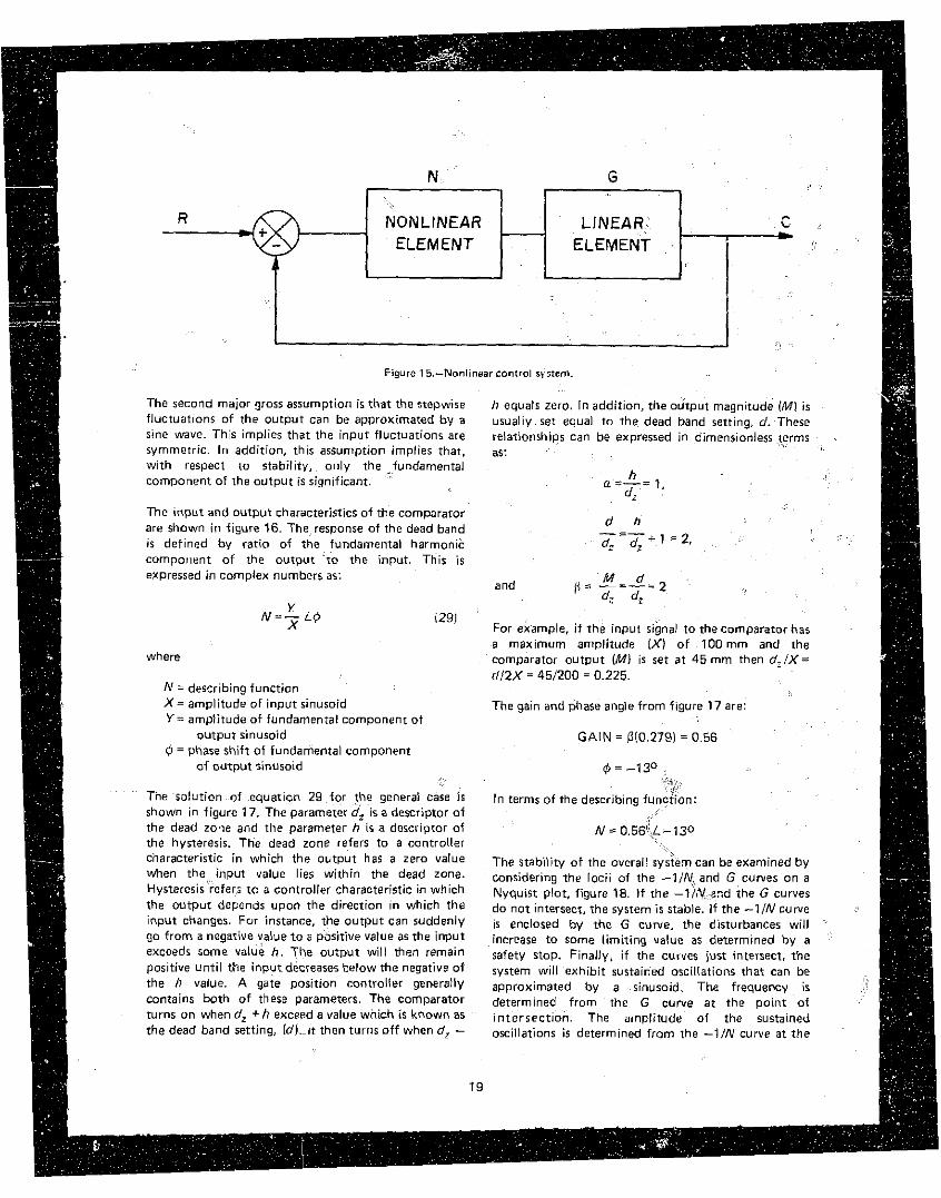
sinusoidal variations at the upstream end of the reach. Neglecting nonlinear effects introduced by the dead band action at the gate, the open-loop responsecan be determined from the/;response characteristics of each element. The gain i s ubtained by multiplication of the gains of each element. The phase anglesare obtained by summing the phase angles. The results of this process for the second reach of the Coalinga Canal are given in table 1.

Closed-loop ~wonse.-#The closed-loop response fur:tion gives the magnitude of the output IC) in terms of the input signal iR) . The closed4oop function can be obtained .from the Nichols diagram in the following manner; First. the values of the opemloop function iGHl and LGH are plotted on the Nichols diayrams, figure 22.

A series of light lines are superimposed on the Nichols diagram. The closed-loop frequency-response curves can be constructed by reading the magnitudes and phase angles on the light lines a t those points where the frequency is known. The results of this process for the second reach of the Coalinga Canal are given in the second and third columns of table 2.

The mathematics upon which this procedure i s based results in frequency characteristics of a unity feedback system. figure 6. However, in most canal controllers. the response characteristics are. not equal to unity for all frequencies. Therefore, to obtain the actual closed-loop response, it is necessary to multiply the

Table 1 .-Rewonse Characteristrcs, Second Reacll, Coalinga Canal

ement2 1 Water level' 1 canal4 YZ 1 P I 1 $ 1 1 'k 1 @k

-- Open

lGHi

13.6 1.42 0.45 0.58 2.20 0.081 0.109 0.434 0.033

-

LGH

F w r e 2 2 . - O ~ e n - I o o ~ response, second reach. Coalinga Canal.

Table 2.-Closed-Loop Resoonse, Second Reach, Coalinga Canall

LCIR = I ~ F I C - LH 4 ~ 1 1 angles are in degrees.

response, figure 6.

Application of this procedure to the second reach o f the Coalinga Canal results i n the true closed-loop + response. table 2 and figure 23. It can be seen that the ; 6 0

canal is sensitive to disturbances having a frequency of 4 o about0.075cyclesper minute (4.5 c lh l . The amplitude

of the resonant peak is a result oP the method used t o estimate the response characteristics of the canal. This

System Resonance and Stability

Very frequently the concepts of system resonance and system stability are used interchangeably. Strictly

f = 0.075 c/min. speaking. resonance refers to sustained oscillations that occur at the maximum velue of the closed~loop frequency response. Instability, on the other hand, refers t o oscillations which increase in magnitude unti l something i n the real system fail?. The stability of a f system depends upon the system itself and is no t a function of the amplitude of the input t o the system. 0.' ~.- -. . I n ana l yz i ng a system;-- both the resonance characteristics and the werall system stability must be considered.

System resonance.-To examine resonance, the entire system must be considered with regard to disturbances which could have frequencies near the resonant frequency. The most likely sources of disturbances are ~i~~~~ ~3. -C losed. looD ,each, turning off and on of deliveries at regular intervals, Canal.

29

incremental gate operations as a result o f dead band actim, and fluctuations originating outside the reach under consideration. Of these three, the dead band action could he the most critical. Its effect is relatively constant at all discharge values.

The effect of dead band on the system resonance can be illustrated by the second reach of the Coalinga Canal. Using the previously given canal pal-am~ters and equation 28. the maximum frecyency induced by the dead band i s 0.0063 c h i n for a discharge of 2 mz/s. Increasing the discharge t o 7 m ' i s only increases the maximum frequency to 0.0065 c l~n in . From figure 23. i t is obvious that this and all lower frequencies will not excite thc reach into resonance. I f , however, the controller GA IN had heen increased t o 29, the dead band action would Rave caused the reach t o resonate at 0.075 c h i n . This could have created a resonance problem

Svsten? stability.-The system stability can be conveniently analyzed vvith a Nyquist plot. The real and imaginary ualues are corr;puted from the open.!oop characteristics using

Re = ~GH lcos i ( G H i and

lin = iGHl sin L(GH),

Val>k 3. It is clear for the second reach o i the Coalillga C a w tllar the locus of the open-loop transfer fiinction neither encloses the stsbility point (.-1.0) ::nor intersects tl ie locus of the dead banu response function, figure 24. Therefore, tifc second reach i s stab12 and i t wi l l riot exhibit sustairled oscillations due to nordinexities introcl~icec. by tl ie dead band action.

Table 3.-Stability o f Closed-Loop, Second Reach, Coalinga Canal

Frequency, c/min 1 IRe 1 ?lm

transient response. This corresponds with an effective .:. damping ratio of 0.4 t o 0.7. For amplifications greater than 1.5. several overshoots wi l l occur when a step char.ge is input into the system. Additional topics on design and compensation techniques can be found i n the appropriate chapter of Ogata 171.

In the case of tl ie Coalinga Canal, the closed-loop gain at the resonant peak is 1.25, figure 23. According t o the design recommendation, this gain i s acceptable. I n general, the determination of acceptable values for the amplification. resonant frequency, and dead bands is a trial and error process. For each trial, parameters are chosen t o develop a contt-oiler response curve as i n figure 12. Then the required computations a s outlined i n the previous sections are performed t o determine the frequency response and stability characteristics of the system. When acceptable control parameters are developed, they must be tested i n a 'mathematical model which simulates the operation of the entire canal system.

For the second reach of the Coalinga Canal, the chosen values o f gain, reset, and filter time constant apparently rezulted in satisfactory transient response characteristics. This indicates that the canal frequency response characteristics may have been estimated accurately enough for these computations. A n accurate evaluation o f the frequency response characteristics o f any canal reach i s very dif f icult to perform i n the field because the output of the controller i s influenced both by changes i i i the reference input and by disturbances, see Tigure 3.

In general, two means are available for determining the canal frequency response characteristics. The first method involves changing the water surface elevation upstream o f the reach and observins water level changes in the reach. This method is oriented primarily for use with mathematical simulations. For this

gates positioned so that they represent some steadvstate f low condition. Usually a step change is employed. The duration of the step must be chosen to produce all of tl ie frequencies o f interest. In general. the duration of the step should be less than 12f,,,,,l-' .

I m = IGHI si> L (GHI If the maximum frequency expected is about Values of IGHI and L (GH) from table 1. , 0.1 c/min, then the step duration must be shorter than

30

Des~gn Recommendations

In many cases, the designer 1s concerned no t with t l ie f req~ency response, bu t in the response of a system t o t rans ien ts . Ogata 171 recommends that the amplification factor for the closed-loop response shoulcl lie between 1.0 and 1.4 for satisfactorv

LOOP RESPONSE

Figure 24.-Stability analysis, second reach. coalinga canal.

5 minutes. A computer program called HFRES has been developed to calculate the frequency response of a canal using this method, see appendix A.

The second method involves the superposition of sinusoidal variations in the upstream water surface on the normal operation of the system. The response is determined for each frequency through the use of cross correlations between the sinusoidal input and the water surface changes in the reach. This method can be

applied to operating systems without interrupting the Ppcess. Since only phase and amplitude vary as the impressed frequency varies, the process of cross c~rrelation can be applied successively to each canal reach even though only the most upstream pool i s varicp. The disadvantage of this method is that only one frequency at a time can be investigated. A computer Program called HFCOV has been developed t o determine the amplitude and phase characteristics for any inputted frequency, see appendix B.

Bihliograpby I61 Lee, Y. W., Statistical Theory of Communication, John Wiley, 1966.

I11 Buckley, P. S., Techniques of Process Control. John Wile:, and Sons, 1964. (71 Ogata. K., Modern Control Engineering,

Prentice-Hail, 1970.

Del ivery Systems, Na t iona l I r r igat ion [81 Shand, M. J., Final Report-The Hydraulic Filter Symposium, November 1970. Level Offset Method for the Feedback Control of

Canal Checks, Hydraulic Engineering. University [31 Buyalski. C. P. and Falvey, H. T.. Stability of of California. Berkeley, June 1968.

Au tomat i c Canal Systems utilizing the Frequency Response Method, International [91 Shand, M. J.. Final Report-Automatic Association of Hydraulic Research. Symposium Downstream Control Systems for Irrigation on Fluid Motion Stability in Hydraulic Systems Canals. Report HEL-8-4, Hydraulic Engineering with Automatic Regulators, Romania, September

141 Ippen, A. T. and Goda, Y. . Wave Induced [lo1 USBR Water Systems Automation Team, Water Oscillations in Harbors: The solution for a Systems Automation-State of the Art. July Rectangular Harbor Connected to the Open Sea. 1973. MIT Hydrody~:amics Laboratory, Report 59.

[I11 Wail, E. T., Optimized Determination of Control Parameters for Canal Automation, Colorado

[51 Jenkins. G. M. and Watts, D. G., Spectral Analysis U n i v e r s i t y , D e n v e r Center Repor t 5 01 E R 01550, February 1975.

. .

32

FROM INI'UT AN'I) OUTPUT S1G;VAI.S

The {requency response o i a system IS defined as the ratlo of the Four~er Transform of the output from the systvm to the Fourm Transform of the input to the system. Mati-ematically

where

Elf1 = frequency response YlfJ = Fourier transform of output X f f ~ = Fourier transform of input

The system can be represented schematically by a block diagram.

From ;*.h:; expression it can be seen that the lowest frequ&8cy that can be determined is equal to:

Therefore, in any analysis, the sample time must be long enough to determine the lowest frequencies in the signal.

The highest freque,icy that can be determ~ned is:

ftgzoY =(:) Af= ( 2 A W 1 INPUT OUTPUT

SYSTEM - x ( t ) Y ( t ) Therefore, the time interval between samples must be

chosen so that:

For analysis with a digital computer a special form of AT = (2f,,,,,) ~ ' the Fourier Transform must be used. This form is called a discrete finite Fourier Transform and it is F~~ example, i f one wishes to determine the frequency def~ned as: response of the first reach of the Coalinga Canal, i t i s

necessary to determine the Fourier Transforms of the input and outputs to the canal. Using the computer requires that the input and output signals be d~girtred.

n = At-1 The frequency rahge of interest is:

%nAf l =- T "' C X ( ~ A T ] e i2n(~nAf ) (nAT)

11 = o f,,,i,, = 0.001 c h i n

f,,,,, = 0.5 c h i n

m = O , l , ..., N-1 For t h ~ s range, the sample tlme T must be,

Slnce Af =Land T = NAT, the expression can also NA T

be wr~t ten as. T = f,,, ,,, ' = 1000 m ~ n

AT= G2fm,,)-' = 1 min

The number of samples i s therefore:

The computer program works only on radix-2 numbers of input, that is. 2 t o an integer power. Therefore, the number of samples must be adjusted to:

This adjustment causes the lowest frequency analyzed to become:

To determine the frequency response of a system any type of input signal can be used. That is, it can be periodic, random, or a transient. However, it must contain all frequencies of interest. Jenkins and Watts 151 show that the frequency response is equal to the Fourier Transform of an impulse applied to the system.

system and then transform the output. An impulse is created by setting all input signals equal to the same value except for the first value.

' I If the system being analyzed is linear, the frequency response i s unique. For nonlinear systems the response is a funcrion of the input. Since canals are nonlinear systems, the frequency response can be expected t o vary as the discharge in the canal i s varied.

Therefore, the recommended method of determining the canal response is:

0 Establish a discharge in the canal Quse the depth upstream of the reach under study t o undergo a step change at r = 0 Set a new discharge.

The latter two steps are repeated for the full range of discharges anticipated.

T o f a c i l i t a t e t he determinat ion o f the frequency-response characteristics of a system, a wmputer program called HFRES was developed. The listing which follows includes instructions for its use.

74/74 OPT.1 F T N u. 6 t 4 2 3

PROGRAH H F R E S ~ H F S I G ~ P L F I L E . O U T P J T T T A P E ~ = ~ F J I G G T A P E ~ = O ~ T P U T I

T H I S PKOGKAH OETERHINtS THE FRE'AUENCI RESPINSE OF A SYSTEI.

FKEQUENCI RESPONSE I S W F I N E O A5 THE ? A 1 1 0 OF THL FOURIER . ~ ~p . TRANSFORM OF r ~ E - o u r P u r OF A s v s T E n T O THE FOURIER TRANSFORM OF THE INPUT. THE FREOJCNCV PEJFONSE OF A S I S T E M I S UNIQUE I F I H C S Y B E T E ? I _ I S LINEAR. I F THE SYSTEH 1 5 NON-LINEAR. THE RfSPONSE OEPCYOS UPON TnE INPUT. T d i FREQJENCY RLSPOHSE G I # E N 61 r m s P R O G X A ~ IS THE CONTINUOUS OOUBLE-SIDED INTEGRAL TkANSFORM, ALTHOUGH, ONLY P O S I T I ~ L FRE9ULNCIES ARE PRESENTED I h IN THE OUTPUT. TO OBTAIN THE SINGLE-SIO~ OISCRETL SPECTRUII IAHPLITUOES AND PHASES OF A SIN: S i R I E S I I T I S NLCESSARI T O ? U L T L P . L I ~ r ( i . A H P L I T U J i S 8 1 2 . / I H O U T * D E L T l ~

TO OETERHINE TnE FREUUiNZY QESPJNSt OF A SYSTEH. THE I N P U T SIGN& _HUST-UAlE A FREQUENCI S P X T R U n I N T i E RANGE OF INTEREST. ONE GOOD INPUT SIGNAL IS AN IMPJLSE. TnE IHPULSE HAS ONE FIXEO VALUE A T ZERO r m AND ANJTHLR FIXED VALUE FOR ALL OTH.ER.LI?ES. AN IHPULSE WHICH PPOOUCES A J N I T AMPLITUDE A T ALL FRECUENCIES CAN a: ACHIEJED a * ~AKING TUE ZERO TINE ~ A L U E EQUAL T O LIOELT A M O ALL x n ~ e AHPLIIUDES EQUAL T O zERO,.LF_InE INPUT 1s AN I n p u L s r . r o u nus1 INFORM r n E COMPUTER THROUGH THE -1PULS:- PA2AHCT iR.

IF e>TH.rnx INPUT AND o u r p u r SI;NPLJ HA?£ 4 NOISE COHPONLNT. THE TRANSFOMS W i L L INCLUOE A Ta4NSF02M 3 F THE NOISE. TO HINIMIZE T n x s , A N U H U ~ R OF ~ E C O ~ J S CAN a i T A K E N AND rnr E s r r H h r E s OF THE I N P L T AN0 UTPUT TRANSFOZHS 4VEHAGEO BEFORL THE FRCQUENCI RESPONSE'~IS"OETE%!~NEO.

THE INPUT CONSISTS 0' THE F O L L O 4 I N G I NiN'---THE NUHar?. OF OATA P O I N T S O E F I N I N G THE I N P U T .. . NOUT- THC N u n a ~ n OF D A T A POINTS O E F ~ N ~ N G THE OUTPUI

a 0 1 4 OF THESE YUST BE S A J I X - 2 NJIOERS. THAT I S . 2 K A I S E O TO AN INTECEX POUER GRE4TER THAN 1.

- - -- OLLT- THr T I M E INCREMENT BETYErN OArA P O I N T S I P U L S E - I F THC I N W T I a AN 1HPULSE.SET T H I S =t

OTHERWISL SET = O . - ~ - - -

w L o r : IF NO PLOT IS OESIPEO SET = o I F A PLOT F I L E I S OLSISEO SET = 1 I F A M I C h O F I L H PLOT I S OESIQC.0 SET = 2 .

T H I S I N P U T MUST O i REAO I N A 31+.F0 . * ,21~ FOWAT.

THE w x r DATA IS THE INPUT SIGNAL. ~ O L L O K J av T n E OUTPUT SIGNAL. aorn OF THESE AK PEAO HITH A 1 0 ~ 8 . 4 F O R M A T . EACH A O O I T ~ N L L SET OF I N P U T AN0 OUTPUT OATA HUST START ON A NEW L I N E . THE 0 4 T P I S I N P U T F l O H A F I L C CALLEO HFSIG.

THE OUTPUT CGNSISTS OF I h i INPUT O l r A THE FRLRUENCY IESPONJE OATA A 3 - 0 BODE PLOT OF THE o u r P u r USING UISPLA SOFTWARE

PAGE 1

PAGE

C ROUTINES TO H E A V Y U P 3-0 PLOT C J S V i ,.

- 7 5

C PRUJECTION ON X I PLANE C

T H E FREQUENCY GESPONSE COMPONENTS A i E

P H E 5-T DE;

8. rJ20 3.361 8.190

193.039 199.031 ... >..

2 3.q. 4 11 2 2iy. 36Q

....> t ..::+2. 647 4?'277. 020 ; 309.367 328.260 339.481 346.706 351.855 355.739 358.386

1.691 4.353 b. l+9 3 . a79 9.847 11. i96 13.046 14.516 15.303 17.231

198.501 199.713 200.893 252.001 203.075 214.104 255.0d7 206.034 206.309 207.753 208.546 209.285 209.960 210.603

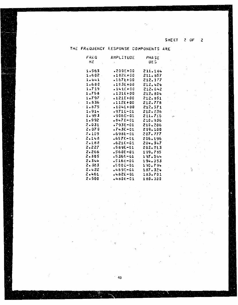
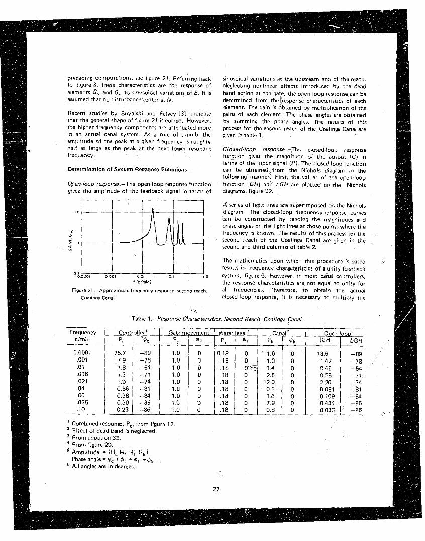
SHEET Z OF 2

THE FRcQUENCY 6.ESPONSE COHPONENTS ARE

FetQ P H A S E H L LIE L

1.563 211.104 1.602 211.657 1.041 212.377 1 .680 212.424 1.719 212.6b2 1.758 212.804 1.797 212. 8 5 1 1.836 212.778 1 .875 212.371 1 .91 r 212.256 1.953 211.715 - 1.992 210.336 2.031 210.206 2.070 209.100 2.109 207.777 2.148 206.196 z . i e e 20+. 3 4 7 2.227 202.313 2.266 199.735 2.305 197.044 2.344 194.353 2.383 130 .794 2.422 187.324 2 4 6 1 183 .701 2.500 100.300

AHPLITUDE

.200E+G0 .18ZL+GO - 1 6 7 t t G O .153EtG0 .141EtOO . 1 3 l E + 0 0 .121E+00 .11ZE+00 . 1 0 4 E t 0 0 - 9 7 1 E - 0 1 .906E-01

847E-01 ,793E-01 . 7 r 3 E - 0 1 , 6 9 8 t - 0 1 r 6 5 7 E - 0 1 r62 l .E-GI ,589E-01 .S60E-01 .53bE-61 . S 1 6 t - 0 1 .EOOi-Di .489E-G1 ,482E-01 e48OE-CI

AT SPI'CIFIC FREQUENCIES BY SUPERIMPOSING A SINUSOIDAL SIGNAL ON THE PROCESS SIGNAL

The principal behind this method involves inputting a Si,, Itl = Ei,, sin {W + Bi) sine wave into the system and measuring the output from the system. From these measurements, the ... s ,,,, ( t ) = E oc,, sin (WT + 82 1 amplitude and phase shifts for the inputted frequency can be determined. If sufficient frequenciesare tested, it is possible t o construct the frequency-response The output signal, which is a water depth in the case of characteristics on a Bode diagram. a canal, consists of the output sinusoid and the process

signal (C = So,,, + N) . The amplitude o f the input signal must be chosen .:L

carefully. I f it i s too large, ihe system will saturate. ~h~ cross correlation $between the input sinusoid and That is, the output will not be proportional to the the output signal equal: I input near the peaks of the sinusoidal wave. In fact, in some cases the output can be constant as the input 4 = iEi,,1IE0,,,1i~~ + 01 continues to follow the sinusoidal variation near the peak. where

On the other hand, i f the input signal is too small. the 0 = 0 2 -0, dead bands in the controller will completely eliminate the effect to the sinusoidal input

A sinusoidal variation can be input into a reach in two ways. The most practical method is to mix the electrical output of a sinusoidal generator with the signal being input into the comparator element of the gate positioner. The second r..;thod is to introduce sinusoidal variation i n the water surface upstream from the reach. I f certain conditions are met, this method will produce a sinusoidal input that i s not influenced by disturbances that occur within the reach, appendix C. The upstream variations can be created by proper cycling of e supply pump, etc.

A system under operation does not have to be stopped to perform this type o f test. I n fact, this method i s designed to be used with operating systems. The theory i s based on the assumption that the ::sinusoidal variations and the process signals simply add together to produce the resultant output signal. Through the use of cross correlations, it i s possible to determine the amplitude and phase shift of the output signal.

Assume that the input and output sinusoids are given by:

If this function is made dimensionless by dividing by E;, , then

The E,,,IEi,, ratio 1s the desired amplitude ratio for use in the Bode diagram and 0 is the corresponding phase angle.

The EOurIEi,, ratio is the maximum value o f the cross correlation function and the phase angle i s determined from the first point (7 = Ol by:

A computer program called HFCOV has been developed to perform the cross correlation. The l~sting which follows includes instructions for its use.

T H I S I S a PfiOGPCH TO C E T E k n I N t THC CO'V4RIANCL F U N C T I O h A N 0 THE C O - S P F ~ T ~ I CF i n 3 SIGMLS x AND I. F ~ C H s I s % a L 1 s OEFINEC 9~ A SL:.IEC O F OPT& P G I H T S Q E G I L N I L E AT T I H C S 9 A N 0 9 fE.O#! SJHE R L F : a i E Z i T I * E . THE T O T A L N U l l a c 2 GF DATA P O I N T S O F F I N I k G OOTH S r 9 1 C S HUSf 'BE .ESS THPN 2CLB. T H r PEOCHAH I S B A S E 0 ON RETHOCS O U T L I N E U I N THE B t O K :

S k I G H b M r C. 0. THF FAST FCURIEr , TEPNSFOHt - I E N 7 I C r HALL . INC.

THE I N F U T C O N S I S T S OF THE FOLLOUING: A- T H E T I W E OISPLbCCMENT F F O H A PEFCKEECE FOR T H E X - S E R I E S OF DATA 0 - T H t T I P C J ISPLACEHENT F 2 O Y P HEFEPEKCL FOR THE Y - S E R I E S OF ObTA NP- T h L LUHRCR 5F 0 4 1 1 D O I N T S C C F I N I N G THE X - S F R I E S PO- T H e L U H e i E CF GAT6 P O I N T S C E F I N I N G THE I - S E R I E S CFLT- *HE 'ir% I N C K ~ H E ~ T RETHEEN DATA POINTS T H I S I L O U T HUST BE 2 E 4 0 ACCOECING TO THE F O R H A 1

2 F 8 . i . 2 1 4 , F u . ~

1 1 THF CO-VARIPNCC FUNCTICL 2 1 T H E C C O S S - C O r i R E L 4 T I O N F U N C T I O N

(CO-VbRLANCZ AV iRAGEO AN0 H 4 0 E O I U C N S I O N L E S S 3 1 S I G N A L O f T E C T I O h HHERE T H E X-OAT* ARE P S I N U S G I O P L I N P U T

bNC 1H; I - D A T A ARE THE OUTPUT I S I N U S O I C P L U S N O I S E 1 F C i 3LTA;LS OF 31, S L E

L E E Y.H. S r b T I Z T I C a L r w o w OF COHHUNICATION

J O H N L I L E I AND SONS 195C1 5C9 Po.

CMCUSk THC TVPE OF A N A L Y S I S D C S I P F D 9 I I N P U T T I h G 1. 2. OR 3 FOR h T I P H I T H 9V I 4 FOPYAT.

T H L Y.--SESIE.S AN0 I -S :RES DATA A F E 2 t A O I N k l O F 8 . 4 FORMAT H I T H A L L O F T H L X - S C ~ I E S O A T & IS KEADFIRST,';~OLLOWEO ALL OF THE I - S E " I i S DATA. \ THE D A T P I S I N F U T F E W 4 F I L E CALLEO H F S I G .

THF OUTPUT C O N S I S T S OF THE I N P U T O P I A f R C ' C O = S P i C t O U k 4NC T H t C O - V A F I i N C L 0 " CROSS-CORCELATION.

O IH 'NT ION X I ~ ~ ~ B ~ ~ Y ~ ~ ~ ~ B I ~ Z R ~ Z O ~ B I I ~ I I ~ O ~ B I I A ~ ~ P I ~ O ~ ~ ~ ~ P H I ~ ~ O ~ ~ ~

I N P U T CF D P T L

REAO~3,11L ,91NP.N0 .0ELT 1 F 0 9 1 4 T I Z F B . 4 ~ 2 1 L ~ F 8 . 4 1

PROGRAU HFCCV 7 + / 7 Q OCTz1 FTN 6 .W-28

RCYO I 3 . 1 5 I N T I P 15 Fomiiix ui-

SEA~13~LlIXlfl~I=lrNP).IYtIl,I=1,Nal 2 F c a ? b T u o F 8 . k l

K = 0

C OUTPUT OF INPUT OATA - 3 W * I T E 1 5 ~ 4 1 1 . 9 . ~ C ~ N O I O E L T ~ N T V P P N P ~ I X l I I , I = 1 N P l . ( Y I I I . I = I j F O ~ ~ P T t I H l r 3 9 x , I I W I ~ P U T OATAf

1 2 7 X . 2 7 ~ 1 1 * € OFFSET OF F I P S T SIGNAL rFR.4/ 2 2 6 X t 2 8 P T I M E OFFSET OF SZCON3 SIGNAL ,FJ.*I 32bX,?7HNU%3iR CF 0 * T l POINTS I N F I I S T SIGNAL . I S / ~ ? 3 i r 3 e R Q U # 9 E P CF OAT1 P J I N T S I N I f C O N O SIGNAL , I & / 537X.7HCfLT4 T 1 ~ 8 . b / A 3 6 X a 1 3 h d h l L Y S I S T Y P i , I$ / 3 / / i 7 K , i 4 1 1 A d b L I S I S TYPE 1 = :O-VAkIANCEf CZ7x.35YANALYSIS TYPE 2 = CCOSS-COkPELATIONf 027X,-Z4k.ANALISIS T Y P i 3 = SIGNAL DETECTION I / / 6.2iX.9HTHF F I R S T . I s . 3 3 H d4TA POINTS A F t THE F I R S T SIGNAL 7 2 7 X , l t * T H c F E H l I N U F ? 4'7 I H t SECOND SIGNAL I I t R L . 1 E F I . l I I

GO r n ! 7 WRITEI? ,PI 8 FOCHP?<1~1~3II~27HNPtNO-l CANNOT EXCCEO EOL8. I

~~*XI . IHPLEASE ' l E 9 I F I YOUR NUMBERS OF INPUT OATD. I C4LL E X I T

PAGE

F T N L.€* \Z I I 1 7 / 5 5 / 2 1 . 14.12.30 PAGE 1

1 2 5 C O I S P L I C t n E N T OF X S I G N A L T O L F F T HANO S I D E OF THE N P O I N T S 7

- C PL-ACEHEYT O F I Z I G N A L TO G i T CORRECT F H & S E ANGLE

1 3 5 C T L - ~ E + A ~ / O E L T r 0 . ~ ~ 0 1 x--rFmTrr h Y I t I = P I N i l P l = N n I h l r l KTST=- KWIN*,N hMAX= h P i - N NHPX= S t N P

1 ~ i H ; € Z . 1 t T S T ; A N 3 . n n b x . ~ r . N O l = MPPX-N,,AK+l hQnN= L Q - N O l , l N o T r = - K - ~ o ~ h + l 0 0 3 8 I = l , N .I= N O l t I - 1 TF( I ;CE; I O Y M ZLI 11 = 1 I JI IFII.GT.YO!~~IZRIII= O. J= T - N ' I T T + l I F ~ I I ~ G E . N O T T J Z R I I I = 0.

33 C O N T I N U E GO TO 4 0

11 %TXq TFl.. N

I F l f . G T . J L l Z R l I I = 1. 33- C7IN n NOF " 0 00 *1 I = I , N

Y I I I ; Z R I I I 4.1 T O N T I N LIE

F O R l b S E TRANSFOPMATTON TO C3MDUTE CO-SPECTRUH I N POLAR FORM

PXOGQCV H F C O Y 7 b / 7 4 CmT=l FTN 4.6t42a 77 /05 /21 . 14.12.30 PAGE 4

1.90 C C COnPUTbTIOI OF TIME OIWLlCEHENT FROM PEFERENCE TIHE S

T I = 9 - 8 "

1 8 5 C C O ~ P U T ~ ~ I O ~ ~ O F CO-SPECTXC FREQUENCY, APPLITUOEI AN0 PHASE r;

f W I E S U B 2 G U i I N r COVF3TES F O M P h G 3NO INVLXS! F O U R I E R TR4N5FC;U5 C S I h G F F T TE:HNl4UET.

THE TChLSFFRt! REQUIRES R L U I X - 2 ? A T & 1 2 TO AN INTEGER POWZRI. B O T H F C W A R O I T I V E - O O R D I N TO F C E W E N C Y - U O ~ * I N I 4ND I N V E R S E I F F E O U E N C I - C C H A I N TO T I l i Z - C 0 H k I : I l T U N S F O I ' I S C D N BE PERFCRPEO. 1'"; G d T h I S ASSU*E(I TO 3 E :DUALLY S ~ A t ~ U A N 0 F E P E T I T I V E AFTER Ir % S I C G G F N OPTA P C I I I T S . THE ObTA I N P U T P l l C OUTPUT FOR T H 5 TdO 3 i E E C T I C N S OF T%AN$FUP,MATICV ALE DS FOLLGYS:

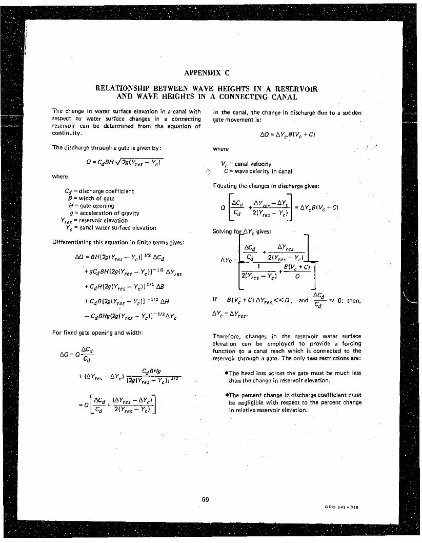
-. AND WAVE HEIGHTS IN A CONNECTING CANAL

The change i n water surface elevation in a canal wi th In the canal, the change in discharge due t o a sudden respect t o water surface changes in a connecting gate movement is: reservoir can be determined from the equation of

AQ = AYcB(Vc + C ) continuity.

The discharge through a gate is given by:

Q = CdBH d 2.d Y,,, - Yc)

where

Cd =discharge coefficient 6 = width o f gate H = gate opening g = acceleration o f gravity

Yrel = reservoir elevation Yc =canal water surface elevation

Differentiating this equation i n finite terms gives:

- CdBHg(2g(Y,,, - Y , ) I - " ~ A Y ~

For fixed gate opening and width:

where

Vc =canal velocity C = wave celerity i n canal

Equating the changes i n discharge gives:

ACd If B(Vc + C ) AY,,, <<Q, and - w 0; then. Cd

AY, = AY,,,.

Therefore, changes i n the reservoir water surface elevation can be employed t o provide a forcing function t o a canal reach which is connected t o the reservoir through a gate. The only two restrictions are:

*The head loss across the gate must be much less than the change i n reservoir elevation.

*The percent change in discharge coefficient must be negligible wi th respect t o the percent change i n relative reservoir elevation.

69 G P O 8 4 3 - 0 1 8

ABSTRACT ABSTRACT

TWO methods are available for determining control Parameters on automated canals. There are the transient-response method and the frequency-response method. Since a There are the transient-rerponre method and the frwuency.rerbonse method. Since a typical canal system ir influenced predominantly by transient inputs, the typical canal ryrtem is influenced predominantly by transient inputs, the transient-response method has been extensively used in the analysis of automated canal tranrient-response method has been extenrively used in the analysis of automated canal systems. The main advantage of the frequency-response method is that the effects of systems. The main advantage of the frequency-response method i s that the effects of Mrying the various control parameterr can be readily visualized and evaluated. The varying the various control parameters can be readily visualized end evaluated. The presently used transient.rerponre method and parameter selection are reviewed. The presently used trsnsient.rerponre method and parameter selection ate reviewed. The basic concepts of the frequency-response method are presented and their application t o basic concepts of the frequency-response method are presented and their application to an automated reach i s illustrated with an example. Two computer programs are given an automated reach is illustrated with an example. Two computer programs are given which can be "red t o determine canal iesponse characterirtics. The rtate-af.theart in which can be used to determine canal response characteristics. The state.of-lhe-art in process control has progrerred sufficiently $0 that both the tranrient.response and process control has progressed rufficiently so that both the tmnsient-response and frequency-rerponre methods of analysis can be wed in a complementary fashion. frequency-response methods o f analysis can be used in a complementary fashion. Employment of only one method in the design of automated rvrtems is, in general. Employment of only one method in the design of automated systems is, in general, wasteful of both computer time and engineering effort. wasteful of both computer time and engineering effort.

ABSTRACT ABSTRACT

Two methods are available for determining control parameters on automated canals. Two methods are available for determining control parameters on automated canals. These are the transient.response method and the frequency-response method. Since a There are the tranrient-response method and the irequencv-response method. Since a typical canal system is influenced predominantly b y transient inputs, the typical canal system is influenced predaminantiv by transient inputs, the transient-response method has been extenrively wed in the analysis of automated canal tranrient-response method has been extensively used in the analyrir of automated calla1 rysteml. The main advantage of the frequency.rerponre method is that the effects of systems. The main sdvantage of the irequency-response method is that the effects of varying the various control parameters can be readily virualized and evaluated. The varying the various control parameters can be readily visualized and evuluated. The presently used transient-response method and parameter selection are reviewed. The presently used tranrient-response method and parameter relectian are reviewed. The basic concepts of the frequency-response method are presented and their application to basic concepts of the irequency-response method are presented and their application to an automated reach ir illustrated with an ,?xample. Two computer programs arc given an automated reach is illustrated with an example. Two computer programs are given which can be used to determine canal respoil~e.~haracterirtic% The state-of-the-art in which can be urcd to determine canal response characteristics. The stated-the-art in process control has progressed sufficiently ro that both the trsnsient-response and process control has progressed rufficiently so that both the tranrient-response and frequency-rerponre methods o f analysis can be used in a complsmentary fashion. frequency.rerponre methods of analysis can be used in e complementary fashion. Employment of only one method in the design of automated systems is. in general, Employment of only one method in the design of automated ryrtema is, in gcncral, wasteful of both computer time and engineering effort. wasteful of both computer time and engineering effort.

FREQUENCY-RESPONSE ANALYSIS OF AUTOMATED CANALS FREQUENCY-RESPONSE ANALYSIS OF AUTOMATED CANALS Bur Reclam Rep REC-ERC.77-3, Div Gen Res, July 1977, Bureau of Reclamation, Bur Reclam Rep REC.ERC.77-3, Div Gen Res, July 1977. Bureau of Reclamation, Denver, 69 p, 25 fig, 3 tab Denver, 69 p. 25 fig. 3 tab

DESCRIPTORS-I "automation1 *canals/ 'analytical techniques1 *frequency analysis/ DESCRIPTORS-I *automation/ *canals/ 'analytical techniques1 'frequency analysis1 automatic control1 control equipment1 feedbacklcontrol systems automaticcontrol/ control equipment/ feedback1 control systems IDENTIFIERS-/ Coalinga Canal IDENTIFIERS-/ Coalinga Canal

REC-ERC-77-3 Falvey, H. T.

I'REQUENCY-RESPONSE ANALYSIS OF AUTOMATED CANALS FREQUENCY-RESPONSE ANALYSIS OF AUTOMATED CANALS t u r Reclam Rep REC-ERC77-3, Div Gen Res, July 1977, B~~~~~ of ~ ~ ~ l ~ ~ ~ ~ i ~ ~ , Bur Reclam Rep REC-ERC-77-3, Div Gen Res, July 1977, Bureau of Redamation, Denver, 69 p, 25 fig, 3 tab Denver. 69 p, 25 fig. 3 tab

DESCRIPTORS-/ 'automation/ *canals/ 'analytical techniques/ *frequency DESCRIPTORS-I 'automation1 *canals/ "analytical techniques1 *frequency analysis/ automatic controV control equipment1 feedbacklcontrol systems automatic controll control equipment1 feedback1 control systems IDENTIFIERS-/ Coalinga Canal IDENTIFIERS-/ Coalinga Canal