1

Analysis Of Behavioural Data

After correction for row total:Transition Rate

Transition Rate

Ethogram Courtship Behavior(Stickleback)

Ethogram Courtship Behavior(Stickleback)

Ethogram Courtship Behavior(Stickleback)

PCA orFactor Analysis

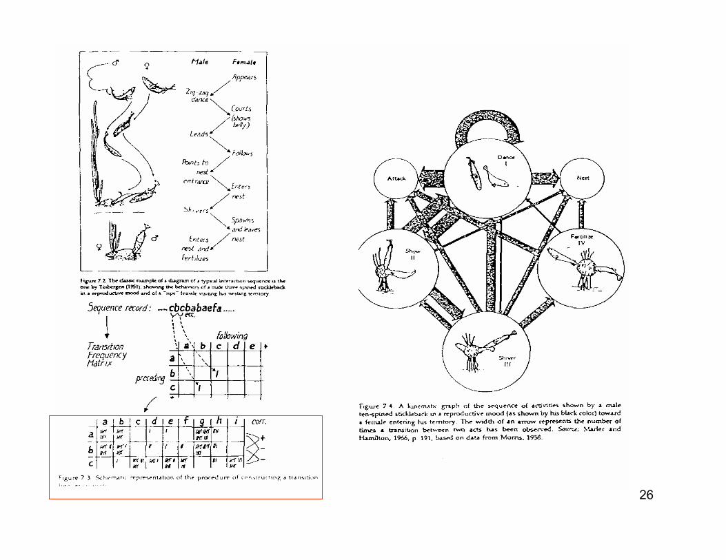
DIMENSION REDUCTIONSchematic representation of the procedure of constructing atransition frequency matrix

Markov Modelling

2

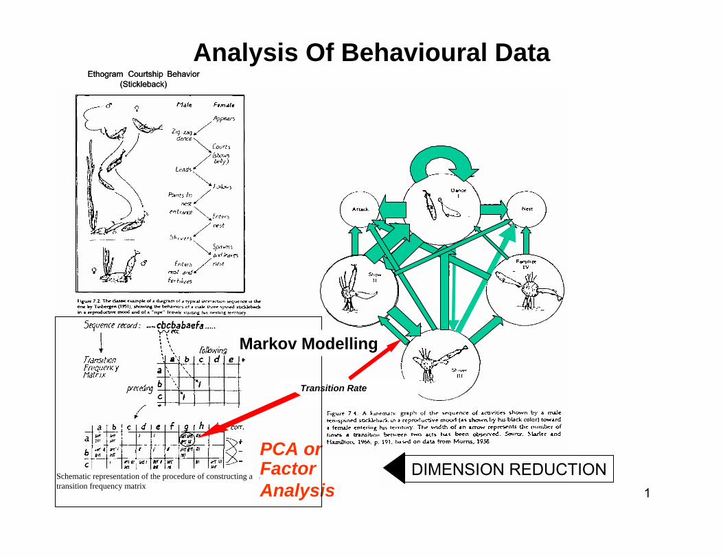
1) Inventory: Decide upon behavioural elements (“Activities”):= setting up an Ethogram

2) Recording: Register the onset and termination timing of the activities.Allows for the computation and assessment of duration and sequence.

3) Summarizing: Cast the ordering of the activities into a Transition Matrix

4) [Dimension Reduction: Combine activities with similar profiles by meansof Cluster Analysis, Factor Analysis and/or Principal Component Analysis]

5) Sequential Analysis: Markov Modelling

Check homogeneity in frequencyand “exponentiality” of duration of single activities*

O.K

Not O.K

Split/LumpActivities

*Only when modelling Continuous Time Markov ChainsSee: P. Haccou & E. Meelis (1992): StatisticalAnalysis of Behaviour. Oxford University Press

Steps in the Analysis

*

3

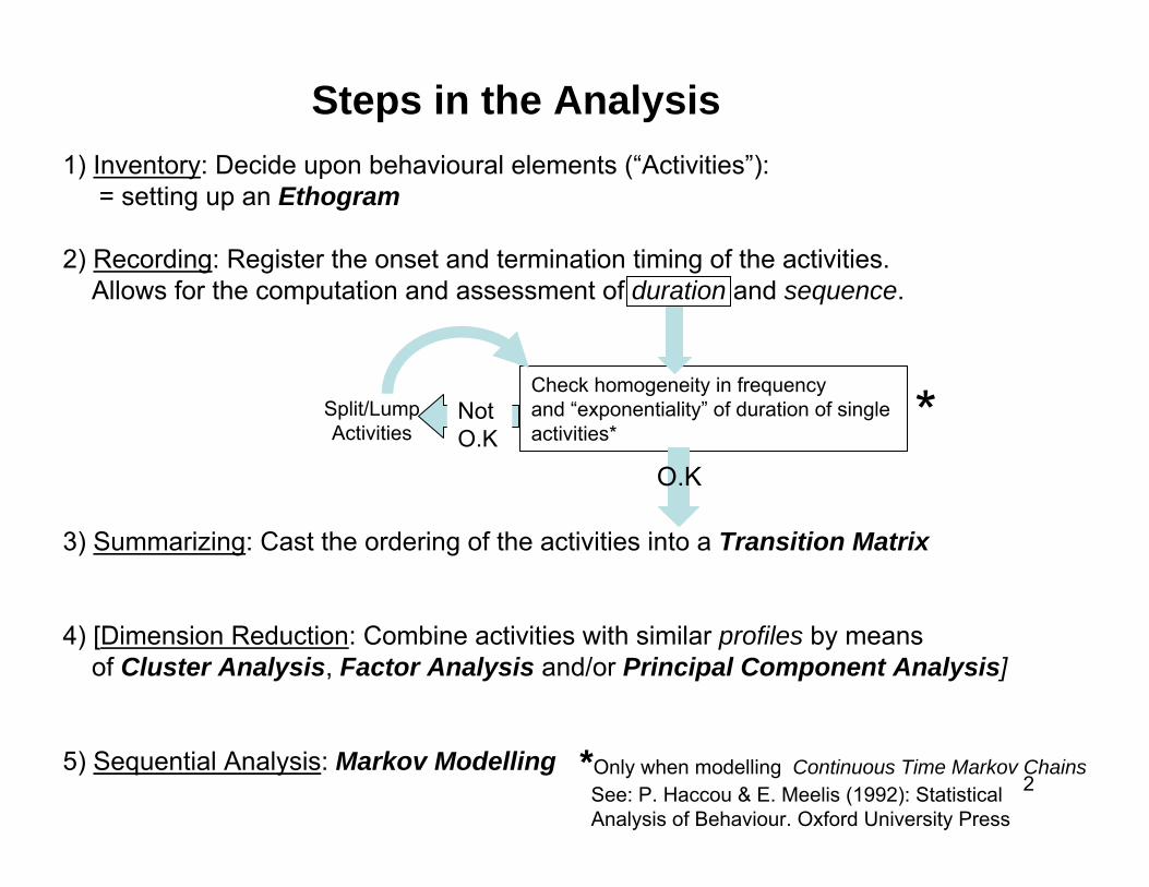
This Course

• Ethogram

• Setting up Transition Matrices

• Simple Markov Model

• Dimension Reduction

Theory(Lecture;

Background Reading)

Application(Practical)

4

Theory• Slides of Lectures

• Literature:

Boekhorst, I.J.A. te(2001). Freeing machines from Cartesian chains. In: “Cognitive Technology: Instruments of Mind” (eds. M. Beynon, C.L. Nehaniv & K. Dautenhahn). Proceedings of the 4th International Conference, CT2001, Coventry, UK. Pp. 95 – 108. Lecture Notes in Artificial Intelligence 2117. Springer, Berlin

Optional:

Bakeman, R. & Gottman, J. M. (1986). Observing Interaction. Cambridge University Press.

Haccou, P. & E. Meelis (1992): Statistical Analysis of Behaviour. Oxford University Press

Lehner, P. N. (1996). Handbook of Ethological Methods. Cambridge University Press.

5

Application

Material (Software):

* seqdepnv: Simple Excel Macro for analysing transition matrices (Markov modelling)

* XLSTAT (Cluster analysis, PCA)

Data:* CD with LEGO robot experiments

6

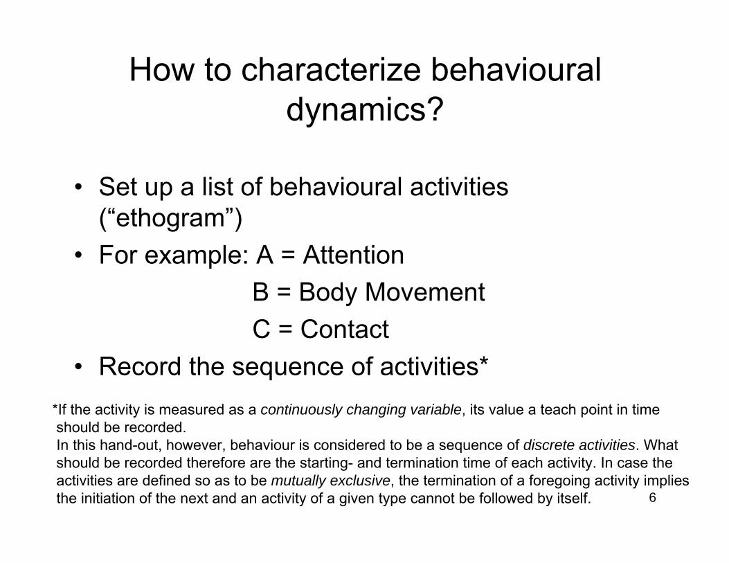
How to characterize behavioural dynamics?

• Set up a list of behavioural activities (“ethogram”)

• For example: A = AttentionB = Body MovementC = Contact

• Record the sequence of activities**If the activity is measured as a continuously changing variable, its value a teach point in time should be recorded. In this hand-out, however, behaviour is considered to be a sequence of discrete activities. Whatshould be recorded therefore are the starting- and termination time of each activity. In case the activities are defined so as to be mutually exclusive, the termination of a foregoing activity impliesthe initiation of the next and an activity of a given type cannot be followed by itself.

7

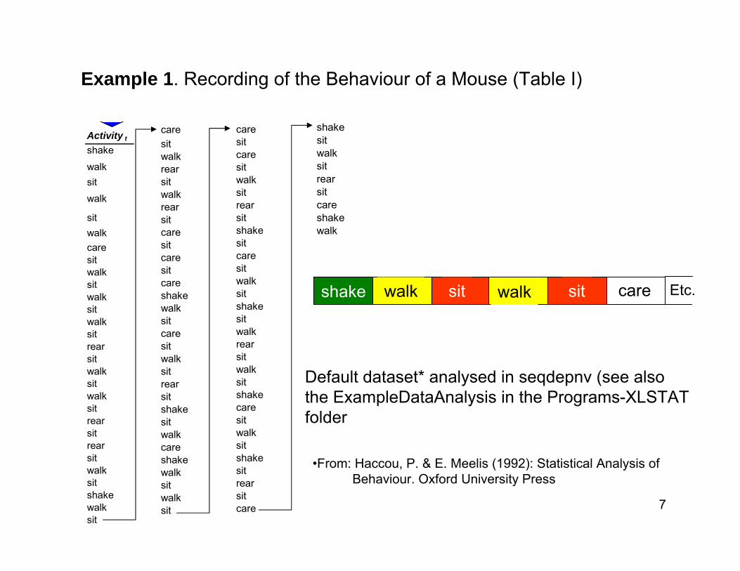
Example 1. Recording of the Behaviour of a Mouse (Table I)

Activity t

shake

walksitwalk

sitwalkcaresitwalksitwalksitwalksitrearsitwalksitwalksitrearsitrearsitwalksitshakewalksit

caresitwalkrearsitwalkrearsitcaresitcaresitcareshakewalksitcaresitwalksitrearsitshakesitwalkcareshakewalksitwalksit

caresitcaresitwalksitrearsitshakesitcaresitwalksitshakesitwalkrearsitwalksitshakecaresitwalksitshakesitrearsitcare

shakesitwalksitrearsitcareshakewalk

•From: Haccou, P. & E. Meelis (1992): Statistical Analysis of Behaviour. Oxford University Press

Default dataset* analysed in seqdepnv (see alsothe ExampleDataAnalysis in the Programs-XLSTATfolder

Etc.shake walk sit walk sit care

8

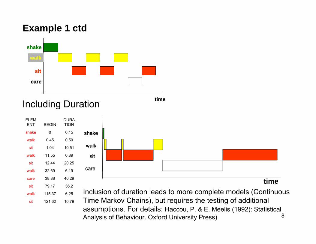
Example 1 ctd

Including Duration

10.79121.62sit

6.25115.37walk

36.279.17sit

40.2938.88care

6.1932.69walk

20.2512.44sit

0.8911.55walk

10.511.04sit

0.590.45walk

0.450shake

DURATIONBEGIN

ELEMENT

time

shake

walk

sit

care

shake

walk

sit

care

shake

walk

sit

care

Inclusion of duration leads to more complete models (Continuous Time Markov Chains), but requires the testing of additional assumptions. For details: Haccou, P. & E. Meelis (1992): Statistical Analysis of Behaviour. Oxford University Press)

shake

walk

sit

care

time

shake

walk

sit

care

time

9

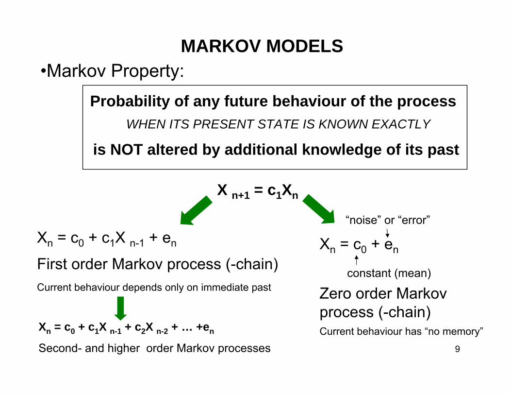
MARKOV MODELS•Markov Property:

Probability of any future behaviour of the processWHEN ITS PRESENT STATE IS KNOWN EXACTLY

is NOT altered by additional knowledge of its past

X n+1 = c1Xn

Xn = c0 + c1X n-1 + en

First order Markov process (-chain)Current behaviour depends only on immediate past

Xn = c0 + en

“noise” or “error”

constant (mean)

Current behaviour has “no memory”

Zero order Markovprocess (-chain)

Xn = c0 + c1X n-1 + c2X n-2 + … +en

Second- and higher order Markov processes

10

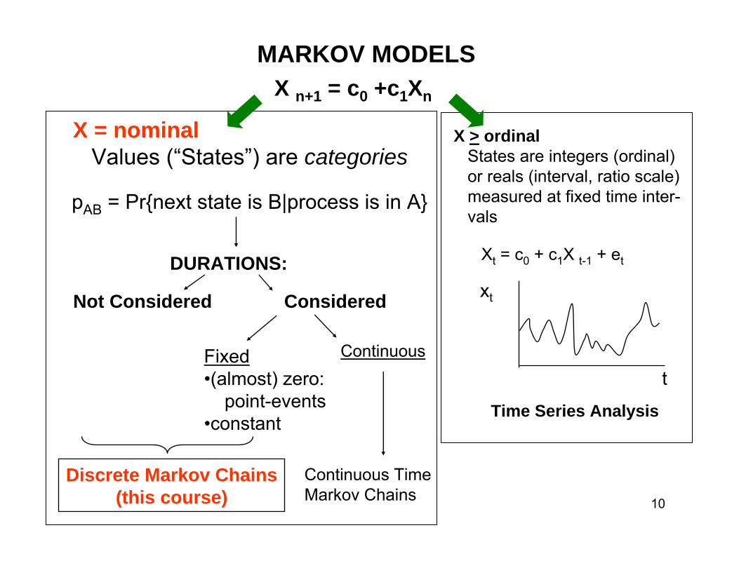
X n+1 = c0 +c1Xn

MARKOV MODELS

X = nominalValues (“States”) are categories

DURATIONS:

Not Considered Considered

Fixed•(almost) zero:

point-events•constant

Continuous

Discrete Markov Chains(this course)

Continuous TimeMarkov Chains

pAB = Pr{next state is B|process is in A}

X > ordinalStates are integers (ordinal)or reals (interval, ratio scale)measured at fixed time inter-vals

t

xt

Time Series Analysis

Xt = c0 + c1X t-1 + et

11

Beh

avio

ural

Sta

te

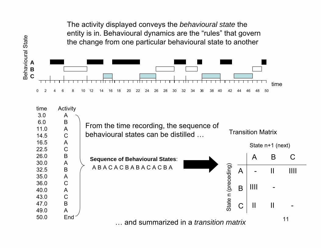
A B A C A C B A B A C A C B ASequence of Behavioural States:

Sta

te n

(pre

cedi

ng)

A B C

A

B

C

State n+1 (next)

II IIII

IIII

II II

Transition Matrix

-

-

-

time Activity3.0 A6.0 B11.0 A14.5 C16.5 A22.5 C26.0 B30.0 A32.5 B35.0 A36.0 C40.0 A43.0 C47.0 B49.0 A50.0 End

ABC

0 2 4 6 8 10 12 14 16 18 20 22 24 26 28 30 32 34 36 38 40 42 44 46 48 50time

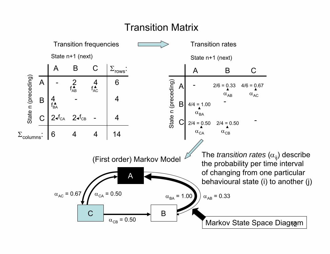
The activity displayed conveys the behavioural state theentity is in. Behavioural dynamics are the “rules” that governthe change from one particular behavioural state to another

From the time recording, the sequence ofbehavioural states can be distilled …

… and summarized in a transition matrix

12

Sta

te n

(pre

cedi

ng)

A B C

A

B

C

State n+1 (next)

2 4

4

2 2

Transition Matrix

-

-

-

Σrows:

6

4

4

Σcolumns: 6 4 4 14

Transition frequencies

Sta

te n

(pre

cedi

ng)

A B C

A

B

C

State n+1 (next)

2/4 = 0.50

Transition rates

-

-

-

4/6 = 0.67

4/4 = 1.00

2/6 = 0.33

2/4 = 0.50

fAC

fBA

fCA

fAB

fCB

αAB αAC

αBA

αCA αCB

A

αAB = 0.33

B

αBA = 1.00αAC = 0.67

C

αCA = 0.50

αCB = 0.50

(First order) Markov Model The transition rates (αij) describethe probability per time interval of changing from one particular behavioural state (i) to another (j)

Markov State Space Diagram

13

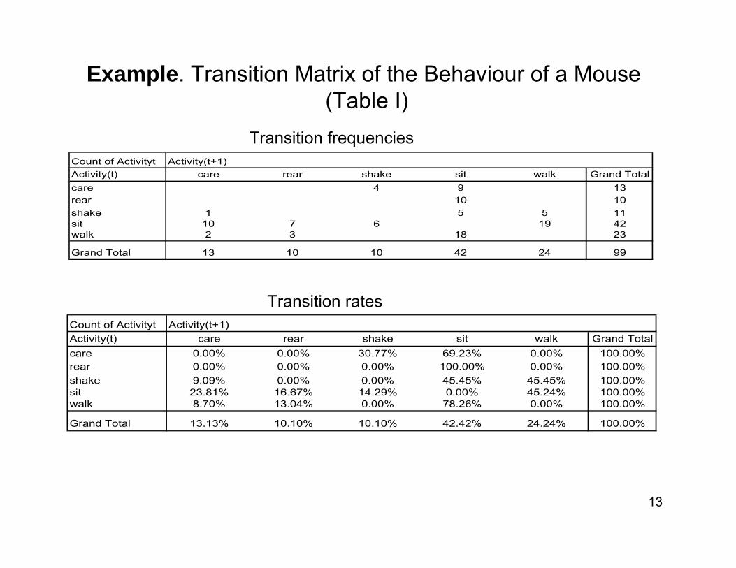
Example. Transition Matrix of the Behaviour of a Mouse(Table I)

Count of Activityt Activity(t+1)Activity(t) care rear shake sit walk Grand Totalcare 4 9 13rear 10 10shake 1 5 5 11sit 10 7 6 19 42walk 2 3 18 23

Grand Total 13 10 10 42 24 99

Count of Activityt Activity(t+1)Activity(t) care rear shake sit walk Grand Totalcare 0.00% 0.00% 30.77% 69.23% 0.00% 100.00%rear 0.00% 0.00% 0.00% 100.00% 0.00% 100.00%shake 9.09% 0.00% 0.00% 45.45% 45.45% 100.00%sit 23.81% 16.67% 14.29% 0.00% 45.24% 100.00%walk 8.70% 13.04% 0.00% 78.26% 0.00% 100.00%

Grand Total 13.13% 10.10% 10.10% 42.42% 24.24% 100.00%

Transition frequencies

Transition rates

14

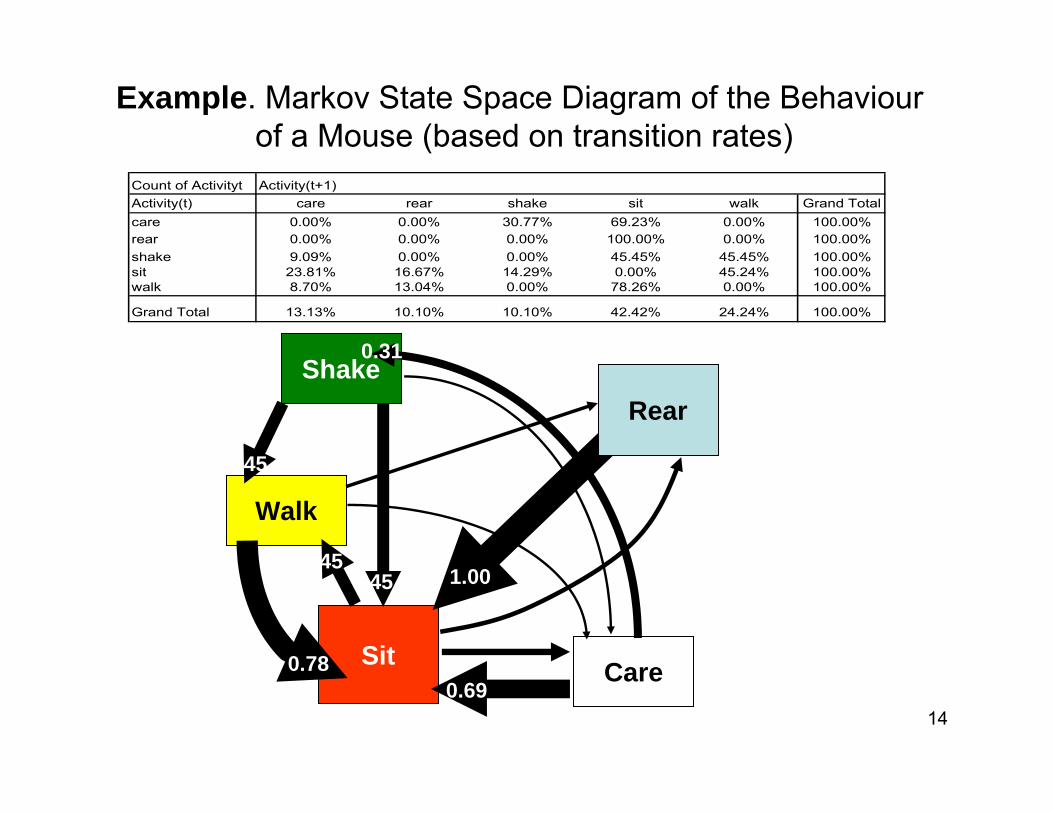
Count of Activityt Activity(t+1)Activity(t) care rear shake sit walk Grand Totalcare 0.00% 0.00% 30.77% 69.23% 0.00% 100.00%rear 0.00% 0.00% 0.00% 100.00% 0.00% 100.00%shake 9.09% 0.00% 0.00% 45.45% 45.45% 100.00%sit 23.81% 16.67% 14.29% 0.00% 45.24% 100.00%walk 8.70% 13.04% 0.00% 78.26% 0.00% 100.00%

Grand Total 13.13% 10.10% 10.10% 42.42% 24.24% 100.00%

Walk

Sit

Shake

Care

Rear

Example. Markov State Space Diagram of the Behaviourof a Mouse (based on transition rates)

1.00

0.690.78

4545

45

0.31

15

Pr , ( )

Pr , ( )

Pr , ( )Pr , ( )

Pr , ( )

AB

A

AB

A

AB

A B in dt A tdt

A in dt A tdt

A B in dt A tB in dt A t

A in dt A t

P

α

λ

αλ

⎡ ⎤→⎣ ⎦=

⎡ ⎤→⎣ ⎦=

⎡ ⎤→⎣ ⎦ ⎡ ⎤= = →⎣ ⎦⎡ ⎤→⎣ ⎦=

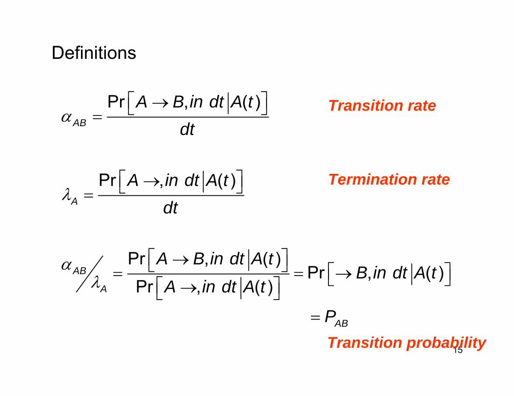
Definitions

Transition rate

Termination rate

Transition probability

16

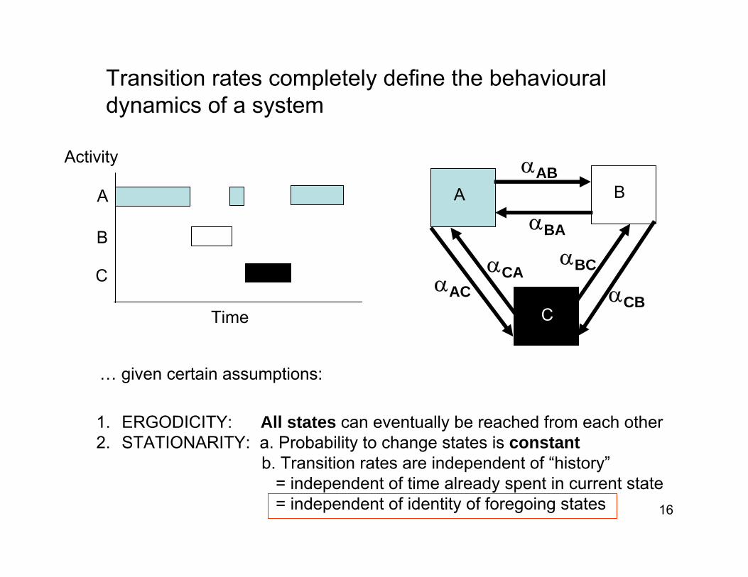
Transition rates completely define the behavioural dynamics of a system

A

B

C

Time

Activity

A B

C

αAB

αBA

αBC

αCB

αCAαAC

… given certain assumptions:

1. ERGODICITY: All states can eventually be reached from each other2. STATIONARITY: a. Probability to change states is constant

b. Transition rates are independent of “history”= independent of time already spent in current state= independent of identity of foregoing states

17

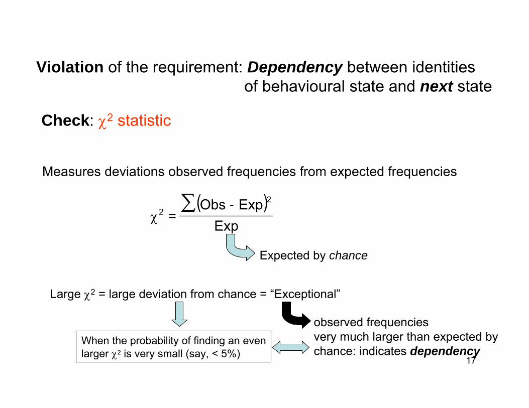
Violation of the requirement: Dependency between identities of behavioural state and next state

Check: χ2 statistic

Measures deviations observed frequencies from expected frequencies

( )Exp

ExpObs=

22 ∑

χ-

Expected by chance

Large χ2 = large deviation from chance = “Exceptional”

observed frequenciesvery much larger than expected bychance: indicates dependency

When the probability of finding an evenlarger χ2 is very small (say, < 5%)

18

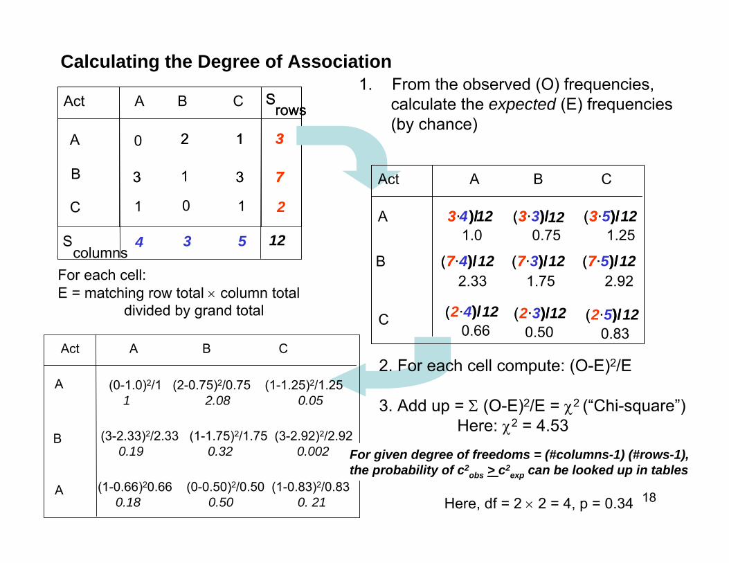
Calculating the Degree of Association

For each cell:E = matching row total × column total

divided by grand total

Srows

2 1 3

B 3 1 3 7

2

Act A B C Srows

A 2 1 3

3 3 7

Scolumns

4 3 5 12

C 1 10

0

Act A B C

A

B

A

(3-2.33)2/2.33 (1-1.75)2/1.75 (3-2.92)2/2.920.19 0.32 0.002

(1-0.66)20.66 (0-0.50)2/0.50 (1-0.83)2/0.830.18 0.50 0. 21

1. From the observed (O) frequencies,calculate the expected (E) frequencies(by chance)

2. For each cell compute: (O-E)2/E

3. Add up = Σ (O-E)2/E = χ2 (“Chi-square”)Here: χ2 = 4.53

(0-1.0)2/1 (2-0.75)2/0.75 (1-1.25)2/1.251 2.08 0.05

For given degree of freedoms = (#columns-1) (#rows-1), the probability of c2

obs > c2exp can be looked up in tables

Here, df = 2 × 2 = 4, p = 0.34

A 3· )/ (3·3)/ (3·5)/12

B (7·3)/12 (7·5)/12

Act A B C

3·4)/12 (3· )/ (3· )/1.0 0.75 1.25

(7· )/ (7· )/(7·4)/12(7· )/2.33 1.75 2.92

C (2·4)/120.66

( · )/ (2·3)/120.50

( · )/ (2·5)/120.83

( · )/

12

19

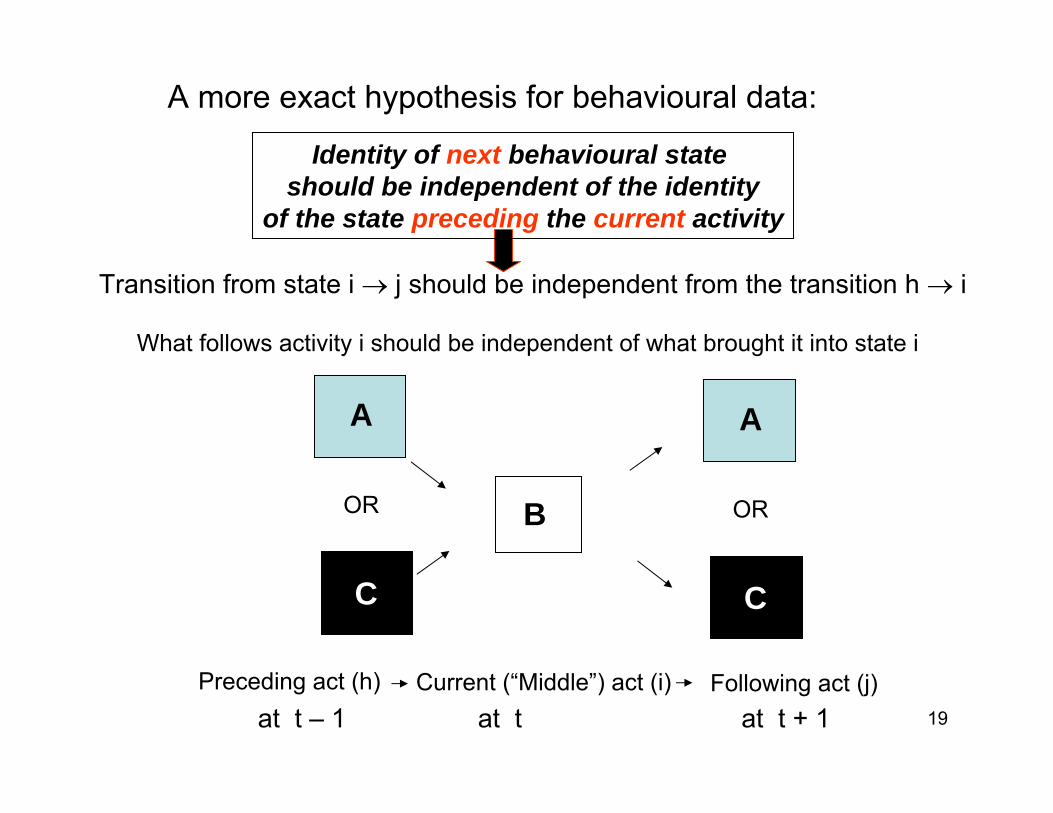
Transition from state i → j should be independent from the transition h → i

What follows activity i should be independent of what brought it into state i

B

A

C

OR

A

C

OR

Preceding act (h) Current (“Middle”) act (i) Following act (j)at t – 1 at t at t + 1

A more exact hypothesis for behavioural data:

Identity of next behavioural state should be independent of the identity

of the state preceding the current activity

20

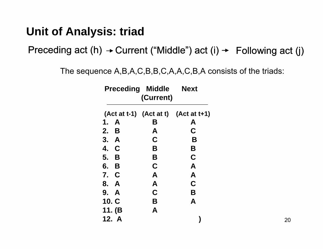
Unit of Analysis: triadPreceding act (h) Current (“Middle”) act (i) Following act (j)Preceding act (h) Current (“Middle”) act (i) Following act (j)

Preceding Middle Next(Current)

(Act at t-1) (Act at t) (Act at t+1)1. A B A2. B A C3. A C B4. C B B5. B B C6. B C A7. C A A8. A A C9. A C B10. C B A11. (B A12. A )

The sequence A,B,A,C,B,B,C,A,A,C,B,A consists of the triads:

21

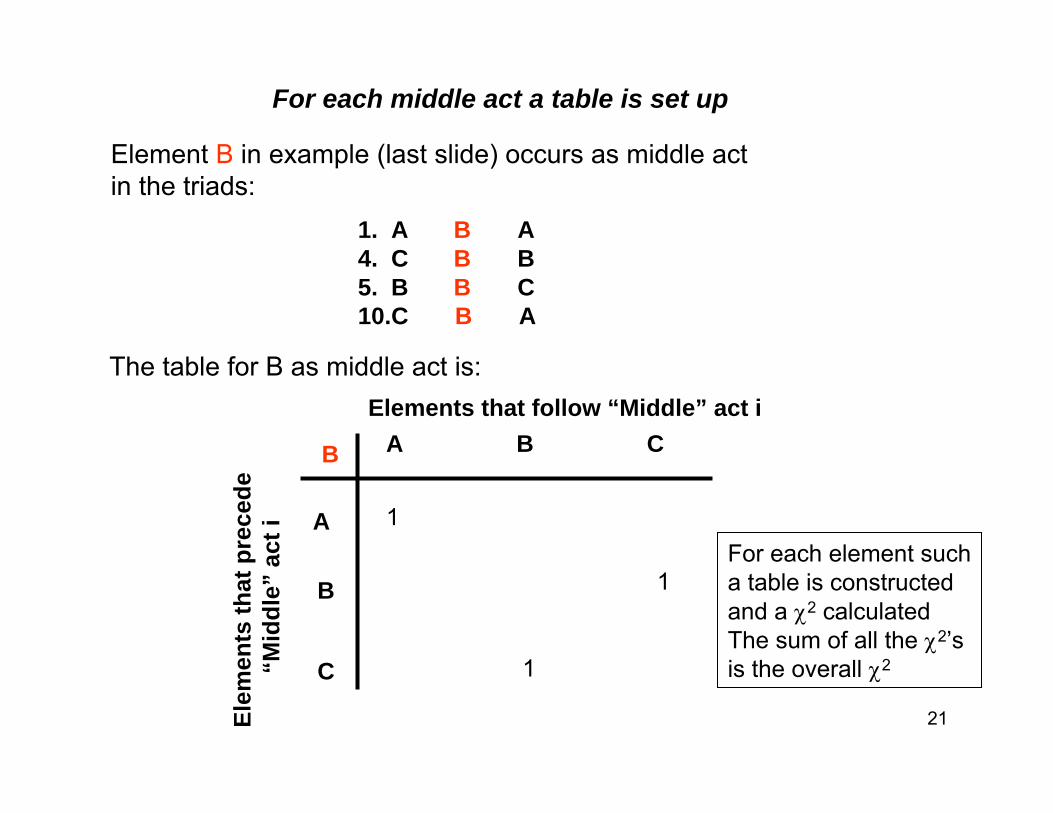
For each middle act a table is set up

Elements that follow “Middle” act i

Elem

ents

that

pre

cede

“M

iddl

e”ac

t i

A B C

A

B

C

Element B in example (last slide) occurs as middle actin the triads:

B

1. A B A4. C B B5. B B C10.C B A

The table for B as middle act is:

1

1

1For each element sucha table is constructedand a χ2 calculatedThe sum of all the χ2’sis the overall χ2

22

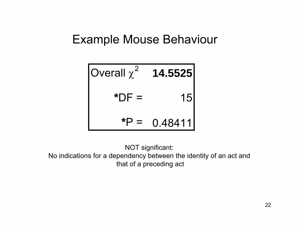
Example Mouse Behaviour

Overall χ2 14.5525

*DF = 15

*P = 0.48411

NOT significant: No indications for a dependency between the identity of an act and

that of a preceding act

23

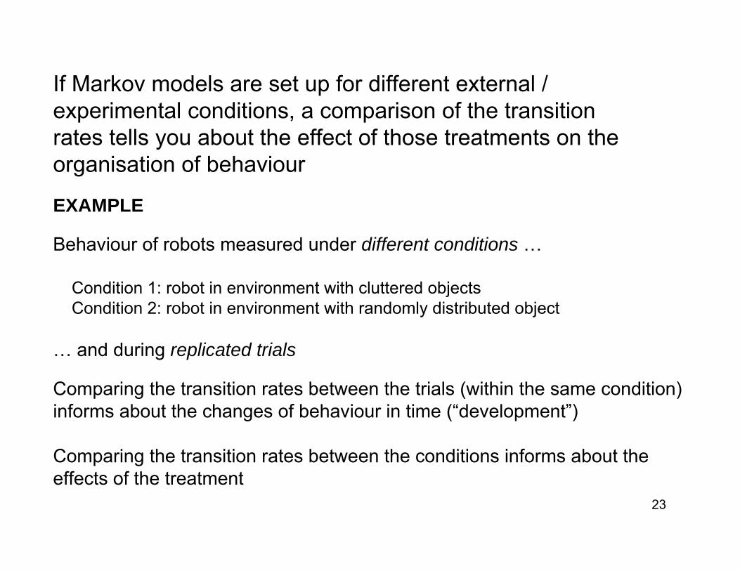
EXAMPLE

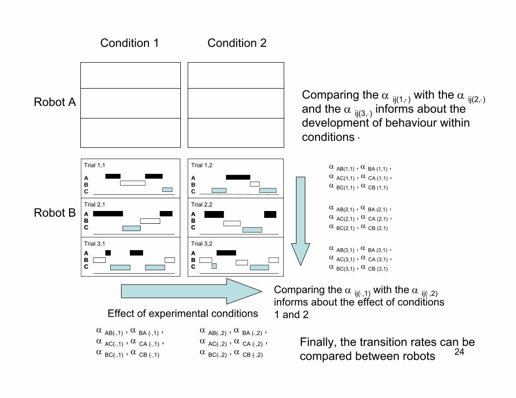
Behaviour of robots measured under different conditions …

Condition 1: robot in environment with cluttered objectsCondition 2: robot in environment with randomly distributed object

… and during replicated trials

Comparing the transition rates between the trials (within the same condition) informs about the changes of behaviour in time (“development”)

Comparing the transition rates between the conditions informs about the effects of the treatment

If Markov models are set up for different external / experimental conditions, a comparison of the transition rates tells you about the effect of those treatments on the organisation of behaviour

24

Robot A

Robot B α AB(2,1) , α BA (2,1) ,α AC(2,1) , α CA (2,1) ,α BC(2,1) , α CB (2,1)

α AB(3,1) , α BA (3,1) ,α AC(3,1) , α CA (3,1) ,α BC(3,1) , α CB (3,1)

α AB(1,1) , α BA (1,1) ,α AC(1,1) , α CA (1,1) ,α BC(1,1) , α CB (1,1)

Condition 1 Condition 2

Effect of experimental conditions

ABC

ABC

ABC

Trial 1

Trial 2

Trial 3

ABC

ABC

ABC

ABC

ABC

Trial 1,1

Trial 2,1

Trial 3,1

ABC

ABC

ABC

Trial 1

Trial 2

Trial 3

ABC

ABC

ABC

ABC

ABC

Trial 1,2

Trial 2,2

Trial 3,2

α AB(⋅,1) , α BA (⋅,1) ,α AC(⋅,1) , α CA (⋅,1) ,α BC(⋅,1) , α CB (⋅,1)

α AB(⋅,2) , α BA (⋅,2) ,α AC(⋅,2) , α CA (⋅,2) ,α BC(⋅,2) , α CB (⋅,2)

Comparing the α ij(1,⋅) with the α ij(2,⋅)and the α ij(3,⋅) informs about the development of behaviour within conditions ⋅

Comparing the α ij(⋅,1) with the α ij(⋅,2)informs about the effect of conditions1 and 2

Finally, the transition rates can becompared between robots

25

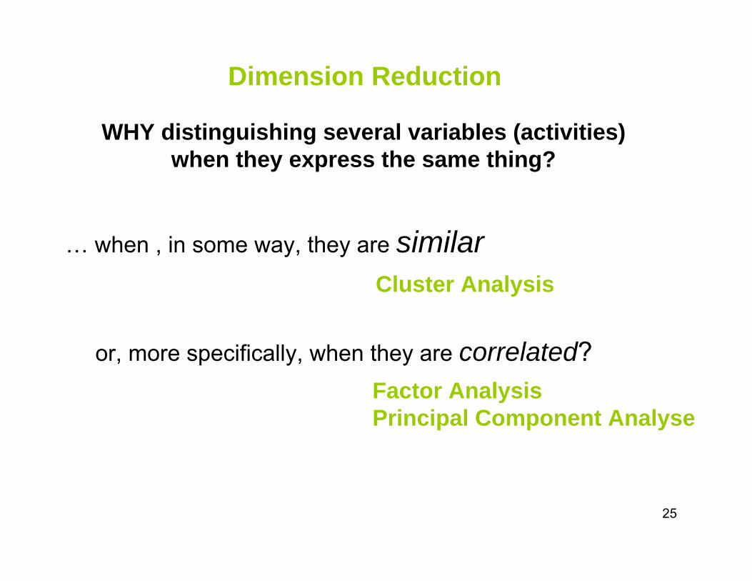
Dimension Reduction

WHY distinguishing several variables (activities) when they express the same thing?

… when , in some way, they are similar

or, more specifically, when they are correlated?

Cluster Analysis

Factor AnalysisPrincipal Component Analyse

26

27

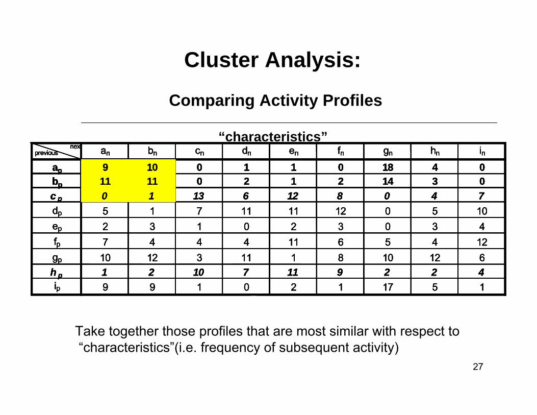
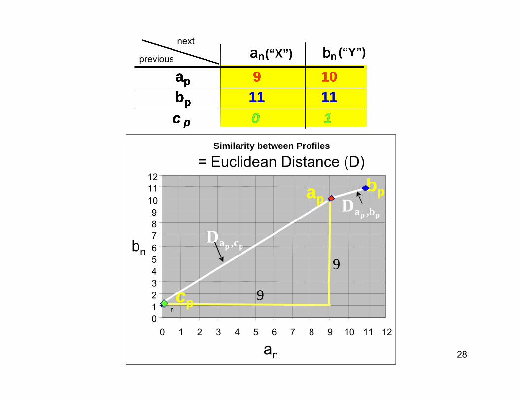
Comparing Activity Profiles

pp b,aD

“characteristics”

Cluster Analysis:

Take together those profiles that are most similar with respect to“characteristics”(i.e. frequency of subsequent activity)

cn dn en fn gn hn in0 1 1 0 18 4 00 2 1 2 14 3 0

13 6 12 8 0 4 7dp 5 1 7 11 11 12 0 5 10ep 2 3 1 0 2 3 0 3 4fp 7 4 4 4 11 6 5 4 12gp 10 12 3 11 1 8 10 12 6h p 1 2 10 7 11 9 2 2 4ip 9 9 1 0 2 1 17 5 1

cn dn en fn gn hn in0 1 1 0 18 4 00 2 1 2 14 3 0

13 6 12 8 0 4 7dp 5 1 7 11 11 12 0 5 10ep 2 3 1 0 2 3 0 3 4fp 7 4 4 4 11 6 5 4 12gp 10 12 3 11 1 8 10 12 6h p 1 2 10 7 11 9 2 2 4ip 9 9 1 0 2 1 17 5 1

previousnext an bn

ap 9 10bp 11 11c p 0 1

previousnext an bn

ap 9 10bp 11 11c p 0 1

cn dn en fn gn hn in0 1 1 0 18 4 00 2 1 2 14 3 0

13 6 12 8 0 4 7dp 5 1 7 11 11 12 0 5 10ep 2 3 1 0 2 3 0 3 4fp 7 4 4 4 11 6 5 4 12gp 10 12 3 11 1 8 10 12 6h p 1 2 10 7 11 9 2 2 4ip 9 9 1 0 2 1 17 5 1

cn dn en fn gn hn in0 1 1 0 18 4 00 2 1 2 14 3 0

13 6 12 8 0 4 7dp 5 1 7 11 11 12 0 5 10ep 2 3 1 0 2 3 0 3 4fp 7 4 4 4 11 6 5 4 12gp 10 12 3 11 1 8 10 12 6h p 1 2 10 7 11 9 2 2 4ip 9 9 1 0 2 1 17 5 1

previousnext an bn

ap 9 10bp 11 11c p 0 1

previousnext an bn

ap 9 10bp 11 11c p 0 1

previousnext an bn

ap 9 10bp 11 11c p 0 1

previousnext an bn

ap 9 10bp 11 11c p 0 1

ap 9 10bp 11 11c p 0 1

28

pp c,aD

Similarity between Profiles

bpan

cn0123456789

101112

0 1 2 3 4 5 6 7 8 9 10 11 12

an

bn

9

9

pp b,aD

pp c,aD

= Euclidean Distance (D)

pp c,aD

Similarity between Profiles

n0123456789

101112

0 1 2 3 4 5 6 7 8 9 10 11 12

9

9

pp b,aD

pp c,aD

= Euclidean Distance (D)

bn

an bn

ap 9 10bp 11 11c p 0 1

an bn

ap 9 10bp 11 11c p 0 1

an bn

ap 9 10bp 11 11c p 0 1

previous

next an bn

ap 9 10bp 11 11c p 0 1

ap 9 10bp 11 11c p 0 1

(“X”) (“Y”)

an

apbp

cp

29

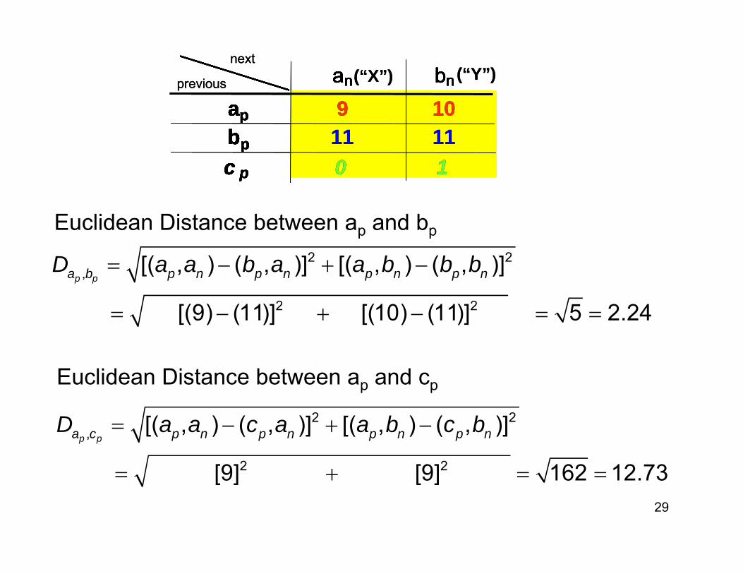
2 2,

2 2

[( , ) ( , )] [( , ) ( , )]

[(9) (11)] [(10) (11)] 5 2.24

p pa b p n p n p n p nD a a b a a b b b= − + −

= − + − = =

Euclidean Distance between ap and bp

Euclidean Distance between ap and cp

2 2,

2 2

[( , ) ( , )] [( , ) ( , )]

[9] [9] 162 12.73

p pa c p n p n p n p nD a a c a a b c b= − + −

= + = =

an bn

ap 9 10bp 11 11c p 0 1

an bn

ap 9 10bp 11 11c p 0 1

an bn

ap 9 10bp 11 11c p 0 1

previous

next an bn

ap 9 10bp 11 11c p 0 1

ap 9 10bp 11 11c p 0 1

(“X”) (“Y”)an bn

ap 9 10bp 11 11c p 0 1

an bn

ap 9 10bp 11 11c p 0 1

an bn

ap 9 10bp 11 11c p 0 1

previous

next an bn

ap 9 10bp 11 11c p 0 1

ap 9 10bp 11 11c p 0 1

(“X”) (“Y”)

30

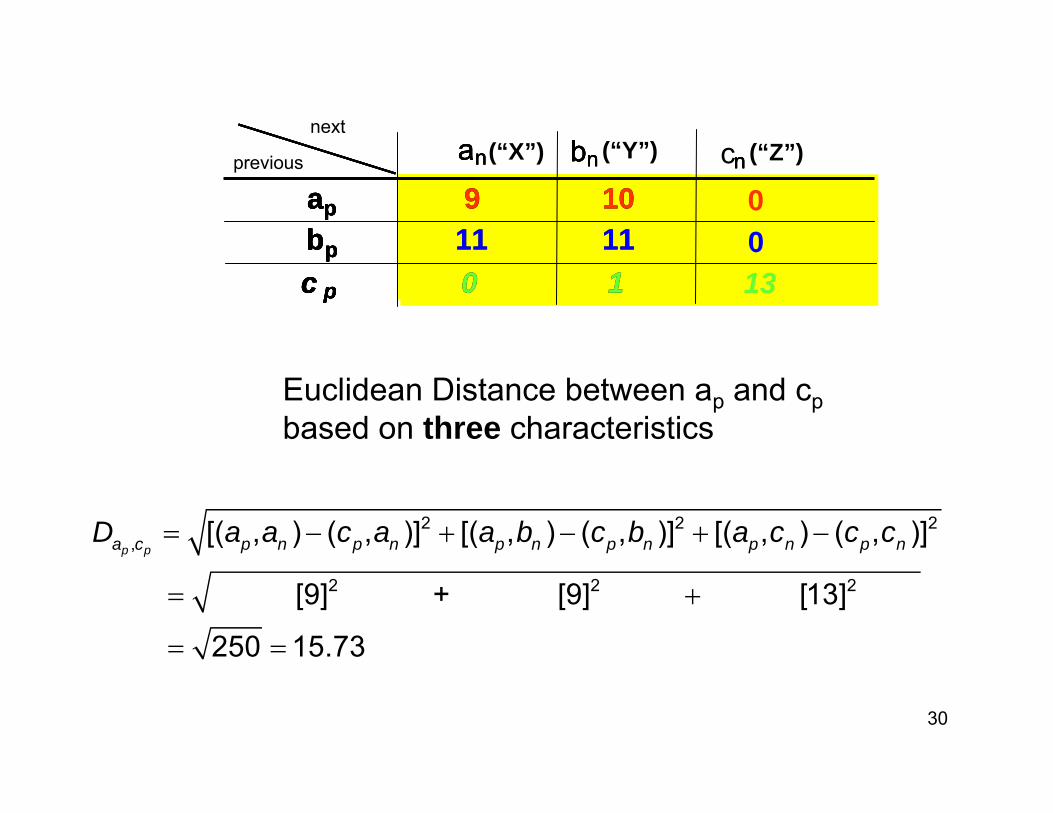
2 2 2,

2 2 2

[( , ) ( , )] [( , ) ( , )] [( , ) ( , )]

[9] + [9] [13]

250 15.73

p pa c p n p n p n p n p n p nD a a c a a b c b a c c c= − + − + −

= +

= =

an

ap 9 10bp 11 11c p 0 1

an

ap 9 10bp 11 11c p 0 1

an

ap 9 10bp 11 11c p 0 1

previous

next an

ap 9 10bp 11 11c p 0 1

ap 9 10bp 11 11c p 0 1

(“X”) bnbnbnbn (“Y”) nncnn (“Z”)

0013

Euclidean Distance between ap and cpbased on three characteristics

31

025.1197117.5499320.6397719.7737228.4429228.284275.3851652.828427i

25.11971022.6936113.076715.93738105.56776424.8193526.85144h

17.5499322.69361018.7616621.9317121.0475725.1396116.1554918.49324g

20.6397713.076718.76166015.1986811.704714.0712520.6639822.67157f

19.7737215.9373821.9317115.19868019.287317.972219.0787821.23676e28.442921021.0475711.704719.2873010.6301527.676730.24897d28.284275.56776425.1396114.0712517.972210.63015028.4429230.23243c5.38516524.8193516.1554920.6639819.0787827.676728.4429205.196152b2.82842726.8514418.4932422.6715721.2367630.2489730.232435.1961520a

ihgfedcba

Euclidean distances

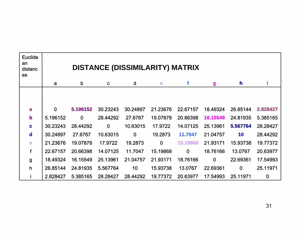
025.1197117.5499320.6397719.7737228.4429228.284275.3851652.828427i

25.11971022.6936113.076715.93738105.56776424.8193526.85144h

17.5499322.69361018.7616621.9317121.0475725.1396116.1554918.49324g

20.6397713.076718.76166015.1986811.704714.0712520.6639822.67157f

19.7737215.9373821.9317115.19868019.287317.972219.0787821.23676e28.442921021.0475711.704719.2873010.6301527.676730.24897d28.284275.56776425.1396114.0712517.972210.63015028.4429230.23243c5.38516524.8193516.1554920.6639819.0787827.676728.4429205.196152b2.82842726.8514418.4932422.6715721.2367630.2489730.232435.1961520a

ihgfedcba

Euclidean distances

DISTANCE (DISSIMILARITY) MATRIX

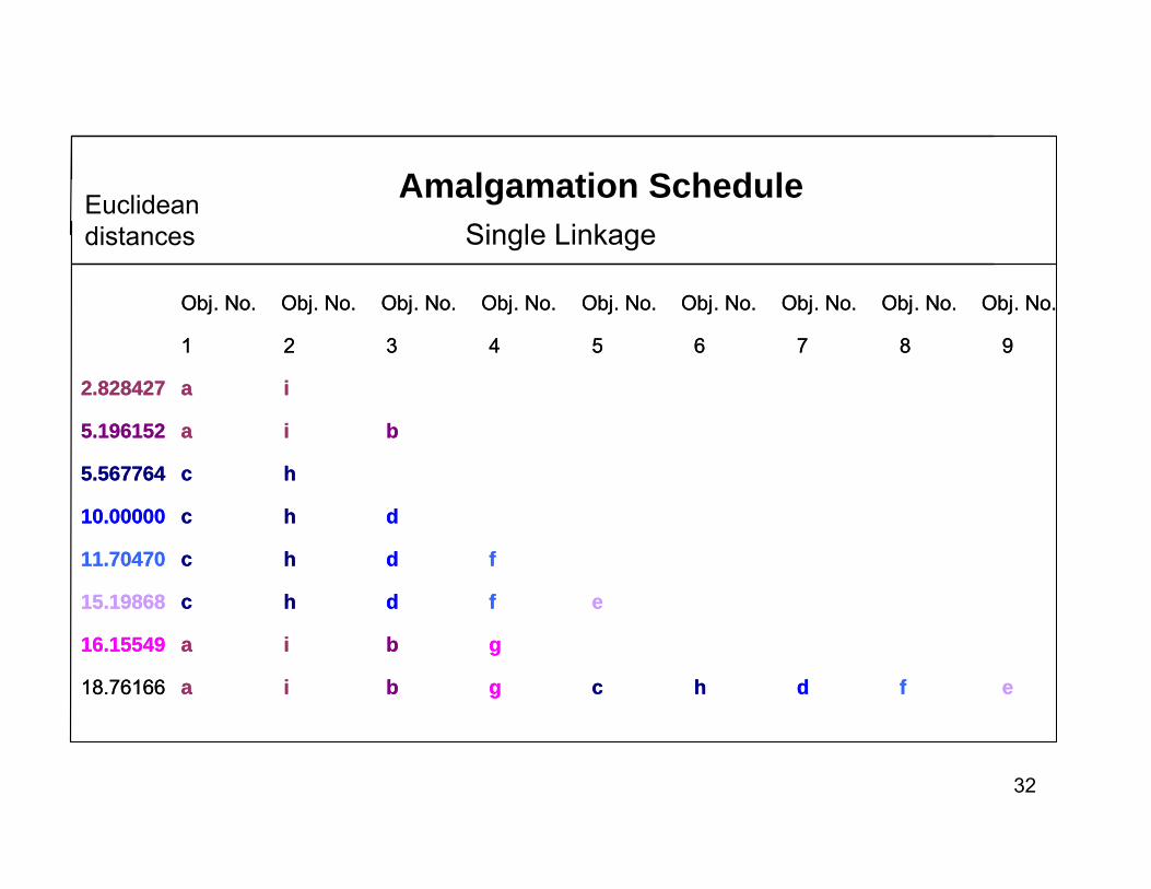
32

18.76166

16.15549

15.19868

11.70470

10.00000

5.567764

5.196152

2.828427

18.76166

16.15549

15.19868

11.70470

10.00000

5.567764

5.196152

2.828427

Obj. No.Obj. No.Obj. No.Obj. No.Obj. No.Obj. No.Obj. No.Obj. No.Obj. No.

efdhcgbia

gbia

efdhc

fdhc

dhc

hc

bia

ia

987654321

efdhcgbia

gbia

efdhc

fdhc

dhc

hc

bia

ia

987654321

Obj. No.Obj. No.Obj. No.Obj. No.Obj. No.Obj. No.Obj. No.Obj. No.Obj. No.

Euclidean distances Single Linkage

Amalgamation Schedule

33

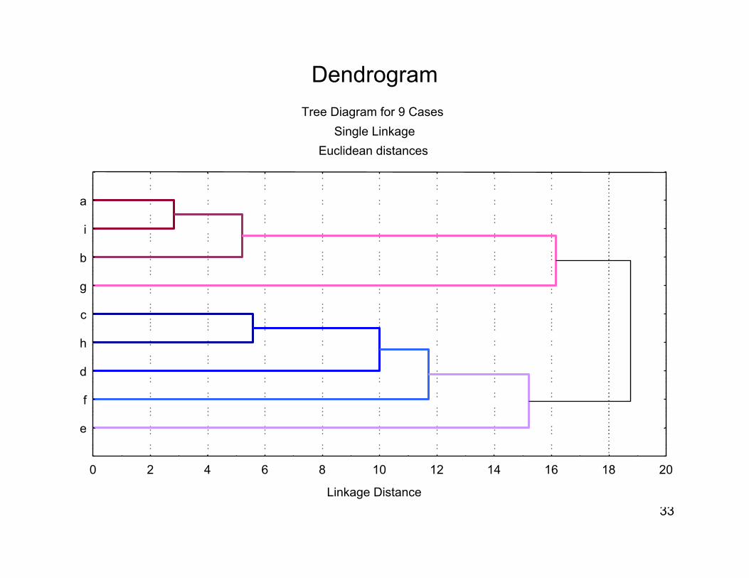
DendrogramTree Diagram for 9 Cases

Single LinkageEuclidean distances

Linkage Distance

e

f

d

h

c

g

b

i

a

0 2 4 6 8 10 12 14 16 18 20

34

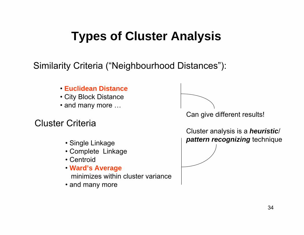
Types of Cluster Analysis

Similarity Criteria (“Neighbourhood Distances”):

• Euclidean Distance• City Block Distance• and many more …

Cluster Criteria

• Single Linkage• Complete Linkage• Centroid• Ward’s Average

minimizes within cluster variance• and many more

Can give different results!

Cluster analysis is a heuristic/pattern recognizing technique

35

Dendrogram

WALK

SIT

SHAKE

REAR

CARE

0 0.05 0.1 0.15

index

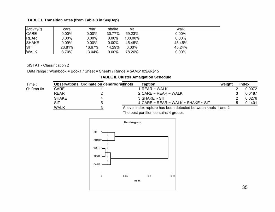
TABLE I. Transition rates (from Table 3 in SeqDep)

Activity(t) care rear shake sit walkCARE 0.00% 0.00% 30.77% 69.23% 0.00%REAR 0.00% 0.00% 0.00% 100.00% 0.00%SHAKE 9.09% 0.00% 0.00% 45.45% 45.45%SIT 23.81% 16.67% 14.29% 0.00% 45.24%WALK 8.70% 13.04% 0.00% 78.26% 0.00%

xlSTAT - Classification 2Data range : Workbook = Book1 / Sheet = Sheet1 / Range = $AM$10:$AR$15

TABLE II. Cluster Amalgation Schedule

Time : Observations Ordinate on dendrogramknots caption weight index0h 0mn 0s CARE 1 1 REAR ~ WALK 2 0.0072

REAR 2 2 CARE ~ REAR ~ WALK 3 0.0187SHAKE 4 3 SHAKE ~ SIT 2 0.0276SIT 5 4 CARE ~ REAR ~ WALK ~ SHAKE ~ SIT 5 0.1401WALK 3 A level index rupture has been detected between knots 1 and 2

The best partition contains 4 groups

36

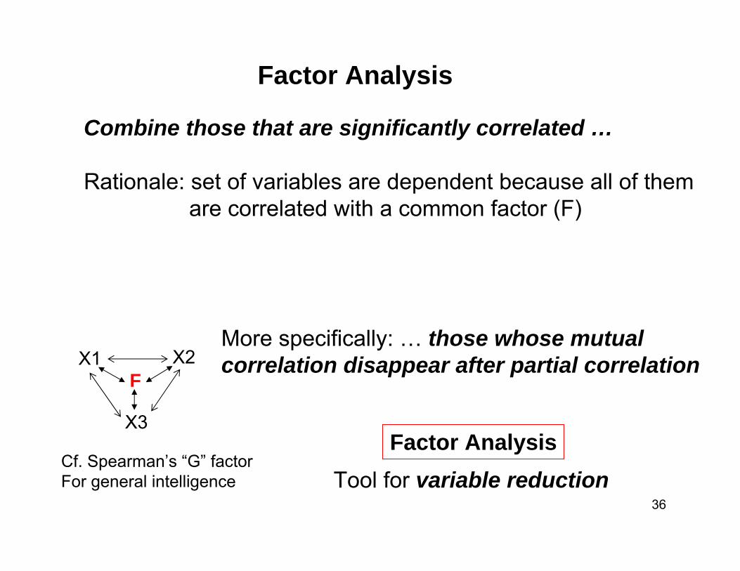
Combine those that are significantly correlated …

Rationale: set of variables are dependent because all of themare correlated with a common factor (F)

X1 X2

X3

F

Cf. Spearman’s “G” factorFor general intelligence

More specifically: … those whose mutualcorrelation disappear after partial correlation

Factor AnalysisTool for variable reduction

Factor Analysis

37

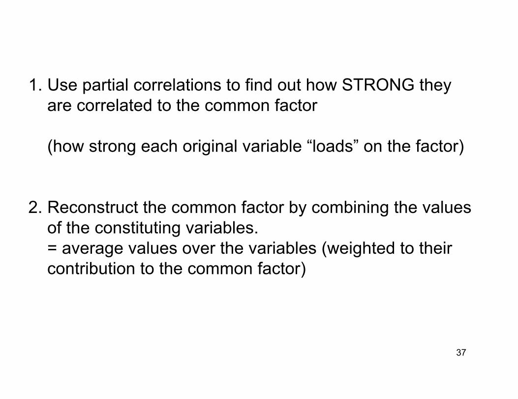
1. Use partial correlations to find out how STRONG theyare correlated to the common factor

(how strong each original variable “loads” on the factor)

2. Reconstruct the common factor by combining the values of the constituting variables.= average values over the variables (weighted to their contribution to the common factor)

38

0

1

2

3

4

5

6

0 1 2 3 4 5 6

X1

X2

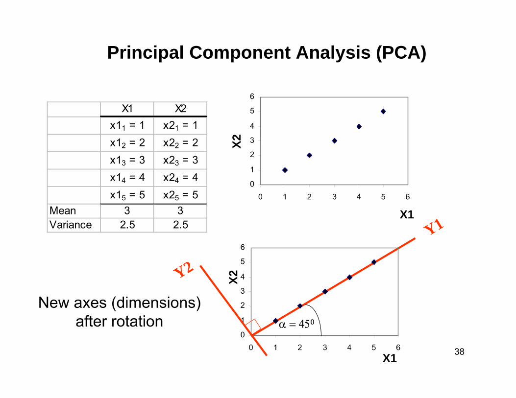
X1 X2x11 = 1 x21 = 1x12 = 2 x22 = 2x13 = 3 x23 = 3x14 = 4 x24 = 4x15 = 5 x25 = 5

Mean 3 3Variance 2.5 2.5

0

1

2

3

4

5

6

0 1 2 3 4 5 6X1

X2Y1

Y2

α = 450

New axes (dimensions)after rotation

Principal Component Analysis (PCA)

39

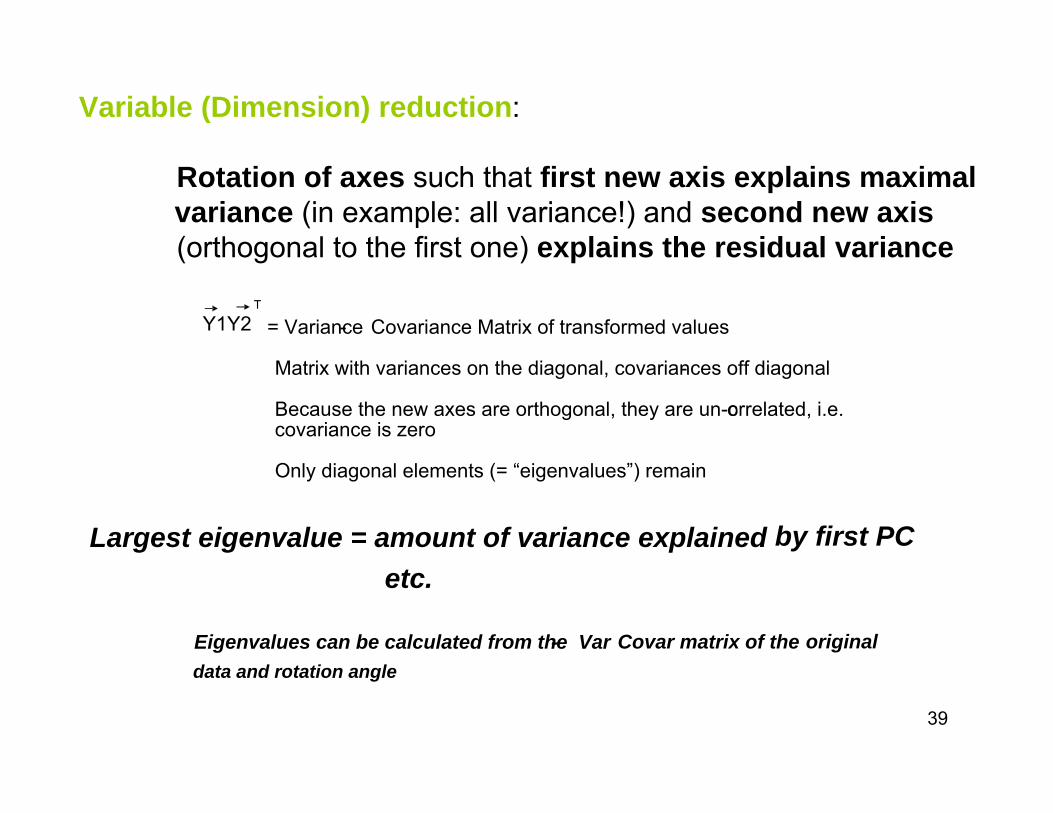
Variable (Dimension) reduction:

Rotation of axes such that first new axis explains maximalvariance (in example: all variance!) and second new axis(orthogonal to the first one) explains the residual variance

Largest eigenvalue = amount of variance explained by first PCetc.

Y1Y2T

= Variance- Covariance Matrix of transformed values

Matrix with variances on the diagonal, covariances off diagonal-

Because the new axes are orthogonal, they are un-correlated, i.e.covariance is zero

Only diagonal elements (= “eigenvalues”) remain

Eigenvalues can be calculated from the Var- Covar matrix of the originaldata and rotation angle

40

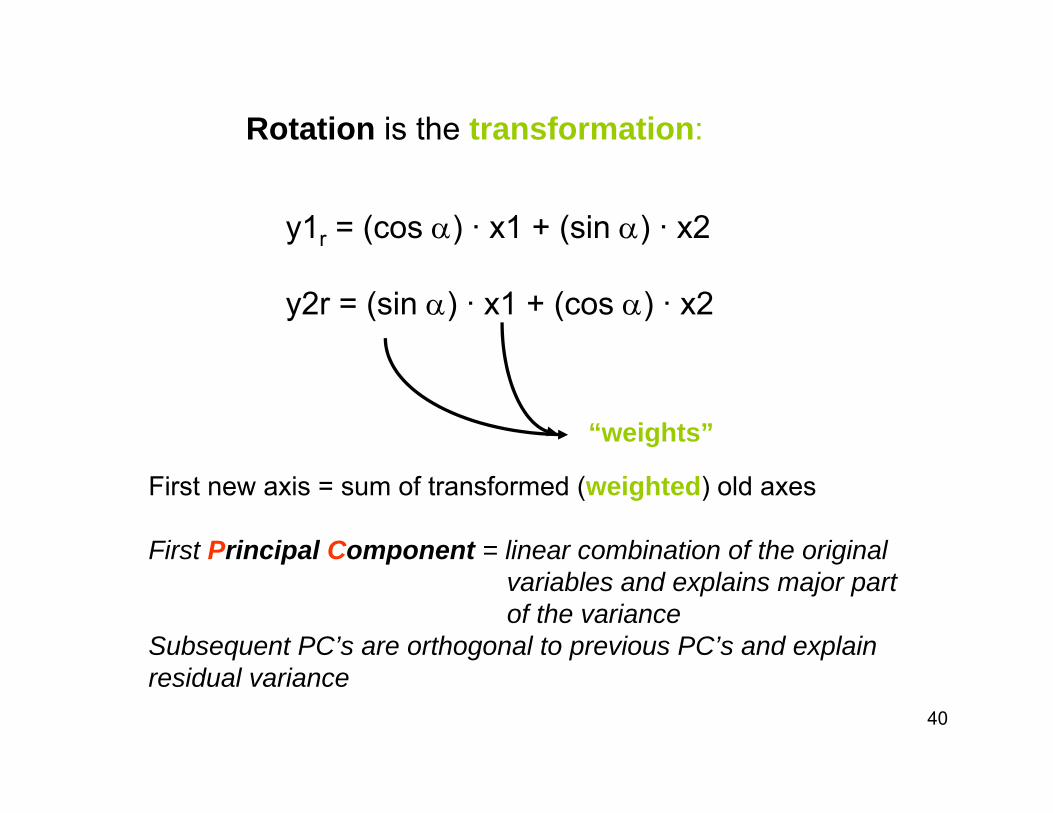
Rotation is the transformation:

“weights”

First new axis = sum of transformed (weighted) old axes

First Principal Component = linear combination of the originalvariables and explains major partof the variance

Subsequent PC’s are orthogonal to previous PC’s and explainresidual variance

y1r = (cos α) · x1 + (sin α) · x2

y2r = (sin α) · x1 + (cos α) · x2

41

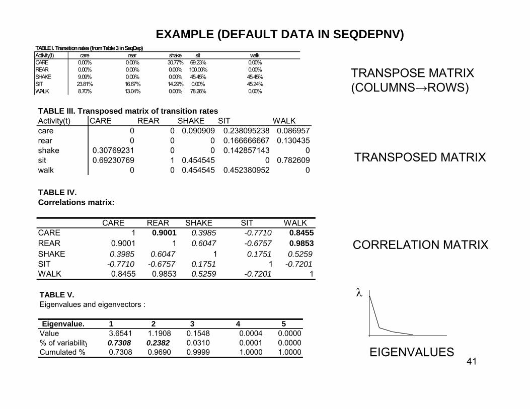
TABLE I. Transition rates (from Table 3 in SeqDep)Activity(t) care rear shake sit walkCARE 0.00% 0.00% 30.77% 69.23% 0.00%REAR 0.00% 0.00% 0.00% 100.00% 0.00%SHAKE 9.09% 0.00% 0.00% 45.45% 45.45%SIT 23.81% 16.67% 14.29% 0.00% 45.24%WALK 8.70% 13.04% 0.00% 78.26% 0.00%

TRANSPOSE MATRIX(COLUMNS→ROWS)

TABLE III. Transposed matrix of transition rates Activity(t) CARE REAR SHAKE SIT WALKcare 0 0 0.090909 0.238095238 0.086957rear 0 0 0 0.166666667 0.130435shake 0.30769231 0 0 0.142857143 0sit 0.69230769 1 0.454545 0 0.782609walk 0 0 0.454545 0.452380952 0

TRANSPOSED MATRIX

TABLE IV.Correlations matrix:

CARE REAR SHAKE SIT WALKCARE 1 0.9001 0.3985 -0.7710 0.8455REAR 0.9001 1 0.6047 -0.6757 0.9853SHAKE 0.3985 0.6047 1 0.1751 0.5259SIT -0.7710 -0.6757 0.1751 1 -0.7201WALK 0.8455 0.9853 0.5259 -0.7201 1

CORRELATION MATRIX

EIGENVALUES

TABLE V.Eigenvalues and eigenvectors :

Eigenvalue. 1 2 3 4 5Value 3.6541 1.1908 0.1548 0.0004 0.0000% of variability 0.7308 0.2382 0.0310 0.0001 0.0000Cumulated % 0.7308 0.9690 0.9999 1.0000 1.0000

EXAMPLE (DEFAULT DATA IN SEQDEPNV)

λ

42

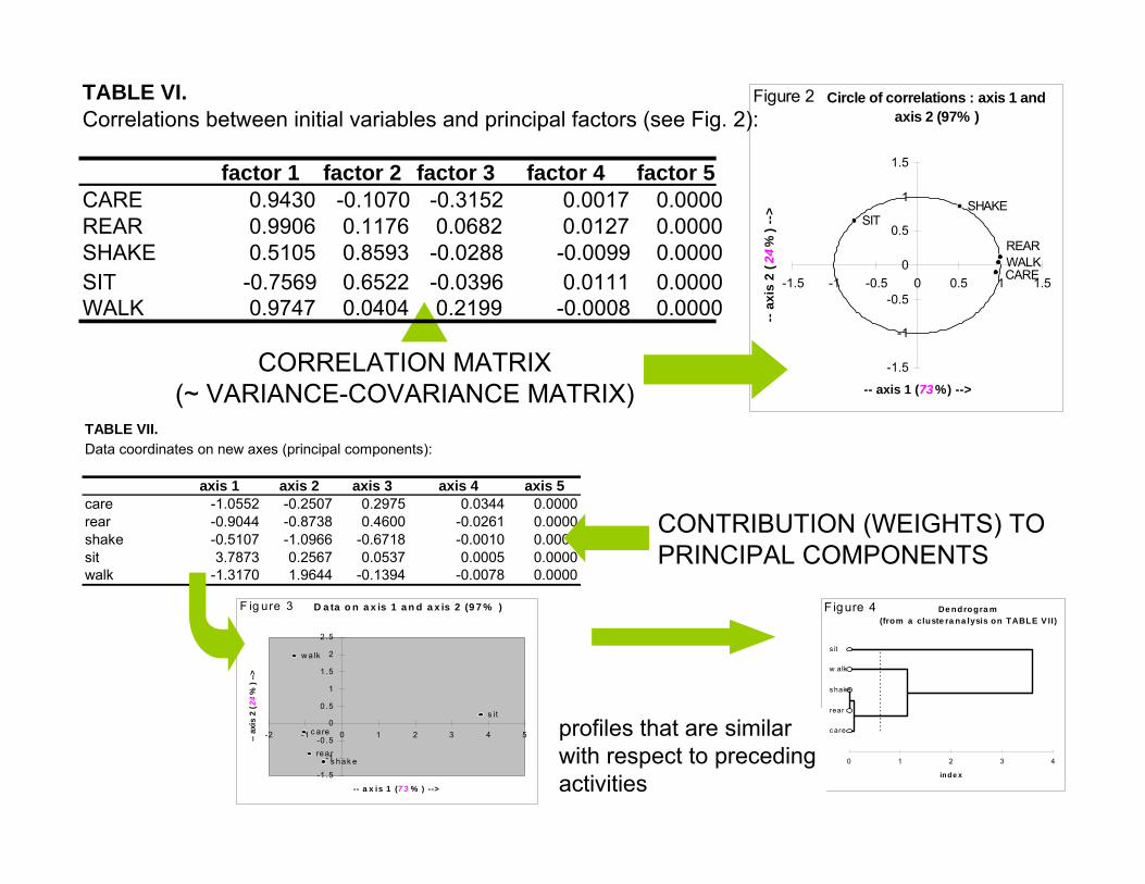
CORRELATION MATRIX(~ VARIANCE-COVARIANCE MATRIX)

Circle of correlations : axis 1 and axis 2 (97% )

WALK

SITSHAKE

REAR

CARE

-1.5

-1

-0.5

0

0.5

1

1.5

-1.5 -1 -0.5 0 0.5 1 1.5

-- axis 1 (73 % ) -->

-- a

xis

2 (2

4%

) --

>

Figure 2

TABLE VII.Data coordinates on new axes (principal components):

axis 1 axis 2 axis 3 axis 4 axis 5care -1.0552 -0.2507 0.2975 0.0344 0.0000rear -0.9044 -0.8738 0.4600 -0.0261 0.0000shake -0.5107 -1.0966 -0.6718 -0.0010 0.0000sit 3.7873 0.2567 0.0537 0.0005 0.0000walk -1.3170 1.9644 -0.1394 -0.0078 0.0000

CONTRIBUTION (WEIGHTS) TOPRINCIPAL COMPONENTS

D a ta o n a x is 1 a n d a x is 2 (9 7 % )

w alk

s it

s hak erea r

c a re

-1 .5

-1

-0 .5

0

0 .5

1

1 .5

2

2 .5

-2 -1 0 1 2 3 4 5

-- a x is 1 (73 % ) -->

-- ax

is 2

(24

% )

-->

F ig ure 3 De ndrogra m(from a cluste ra na lysis on TABLE V II)

w alk

s it

s hake

rear

c are

0 1 2 3 4

ind e x

F igure 4

profiles that are similarwith respect to precedingactivities

TABLE VI.Correlations between initial variables and principal factors (see Fig. 2):

factor 1 factor 2 factor 3 factor 4 factor 5CARE 0.9430 -0.1070 -0.3152 0.0017 0.0000REAR 0.9906 0.1176 0.0682 0.0127 0.0000SHAKE 0.5105 0.8593 -0.0288 -0.0099 0.0000SIT -0.7569 0.6522 -0.0396 0.0111 0.0000WALK 0.9747 0.0404 0.2199 -0.0008 0.0000

43

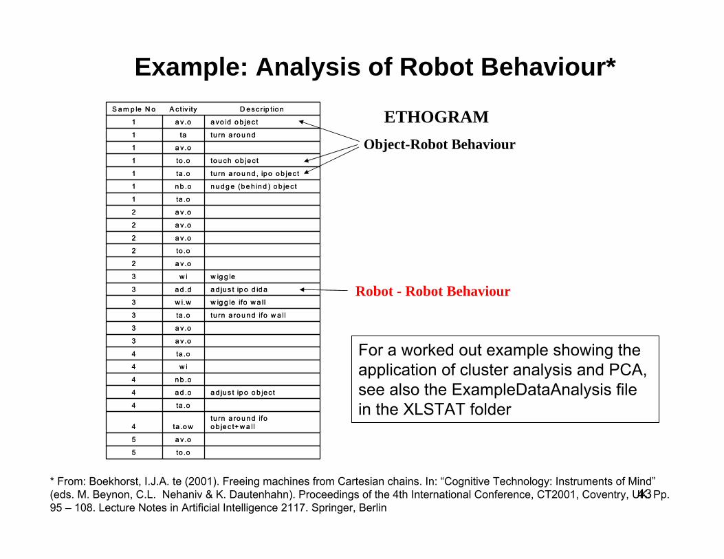
Example: Analysis of Robot Behaviour*

* From: Boekhorst, I.J.A. te (2001). Freeing machines from Cartesian chains. In: “Cognitive Technology: Instruments of Mind”(eds. M. Beynon, C.L. Nehaniv & K. Dautenhahn). Proceedings of the 4th International Conference, CT2001, Coventry, UK. Pp. 95 – 108. Lecture Notes in Artificial Intelligence 2117. Springer, Berlin

to .o5

a v.o5

tu rn a ro u n d ifoo b je c t+ w a llta .o w4

ta .o4

a d ju s t ip o o b jec ta d .o4

n b .o4

w i4

ta .o4

a v.o3

a v.o3

tu rn a ro u n d ifo w a llta .o3

w ig g le ifo w a llw i.w3

a d ju s t ip o d id aa d .d3

w ig g lew i3

a v.o2

to .o2

a v.o2

a v.o2

a v.o2

ta .o1

n u d g e (b e h in d ) o b je c tn b .o1

tu rn a ro u n d , ip o o b jec tta .o1

to u ch o b je c tto .o1

a v.o1

tu rn a ro u n dta1

a vo id o b je c ta v .o1

D e s c r ip tio nA c tiv ityS a m p le N o

to .o5

a v.o5

tu rn a ro u n d ifoo b je c t+ w a llta .o w4

ta .o4

a d ju s t ip o o b jec ta d .o4

n b .o4

w i4

ta .o4

a v.o3

a v.o3

tu rn a ro u n d ifo w a llta .o3

w ig g le ifo w a llw i.w3

a d ju s t ip o d id aa d .d3

w ig g lew i3

a v.o2

to .o2

a v.o2

a v.o2

a v.o2

ta .o1

n u d g e (b e h in d ) o b je c tn b .o1

tu rn a ro u n d , ip o o b jec tta .o1

to u ch o b je c tto .o1

a v.o1

tu rn a ro u n dta1

a vo id o b je c ta v .o1

D e s c r ip tio nA c tiv ityS a m p le N o ETHOGRAMObject-Robot Behaviour

Robot - Robot Behaviour

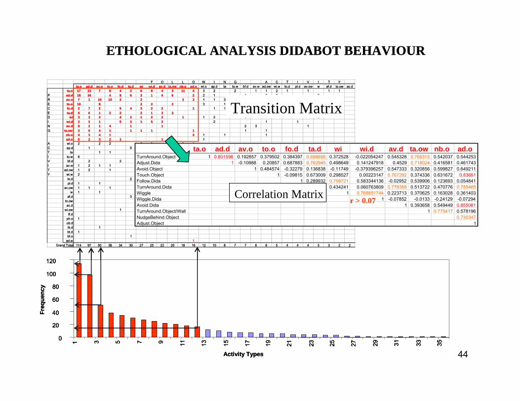
For a worked out example showing theapplication of cluster analysis and PCA, see also the ExampleDataAnalysis filein the XLSTAT folder

44

0

20

40

60

80

100

120

1 3 5 7 9 11 13 15 17 19 21 23 25 27 29 31 33 35

Activity Types

Freq

uenc

y

ETHOLOGICAL ANALYSIS DIDABOT BEHAVIOUR

F O L L O W I N G A C T I V I T Yta.o ad.d av.o to.o fo.d ta.d wi wi.d av.d ta.ow nb.o ad.o wi.o ap.d ta to.w bf.d av.w ad.ow wi.w to.d pl.d av.ow w af.d to.ow ac.d

ta.o 17 23 7 8 4 2 6 8 4 3 11 4 3 2 2 1 1 2 1 1 1 1P ad.d 18 34 4 8 6 3 1 4 6 2 2 1 1 2 2 2R av.o 7 1 10 10 2 2 3 3 1 1 3 3 1 1 1 1E to.o 19 8 2 2 2 3 1C fo.d 2 7 2 5 4 3 2 2 1 1 1 3 1E ta.d 9 6 1 2 2 2 1 3 3D wi 3 3 2 4 2 1 2 2 1 1 2 1 1I wi.d 2 2 1 5 3 1 5 2 2 1 1N av.d 8 2 1 4 1 1 2 3 1G ta.ow 3 6 4 1 1 1 1 1 1 1

nb.o 4 3 4 1 3 1 1 1ad.o 5 2 3 2 1 1 1 1

A wi.o 2 2 2 1 1 1 1 1C ap.d 1 5 2 1 1T ta 1 1 1 1 2 1 1I to.w 6 1V bf.d 2 2 1 1 1I av.w 1 2 1 1 1T ad.ow 1 2 1 1 1Y wi.w 2 1 1 1

to.d 2 1 1pl.d 1 1 1 1

av.ow 1 1 1 1w 1 1 1

af.d 3to.ow 1 1ac.d 1

wi.ow 1tf.d 1

ph.o 1ob.d 1lb.d 1bt.d 1bf.o 1

ad.w 1Grand Total 114 97 50 38 34 30 27 25 22 20 18 16 12 10 8 7 7 6 6 5 4 4 4 3 3 2 2

Transition Matrix

ta.o ad.d av.o to.o fo.d ta.d wi wi.d av.d ta.ow nb.o ad.oTurnAround.Object 1 0.801598 0.192857 0.379502 0.384397 0.698898 0.372528 -0.022054247 0.545328 0.769315 0.542037 0.544253Adjust.Dida 1 -0.10988 0.20857 0.687883 0.762945 0.498649 0.141247918 0.4529 0.718024 0.416581 0.461743Avoid.Object 1 0.484574 -0.32279 0.136838 -0.11749 -0.379396257 0.547333 0.320856 0.599827 0.649211Touch.Object 1 -0.09815 0.673009 0.298527 0.00223147 0.767292 0.374336 0.631672 0.83651Follow.Dida 1 0.289932 0.758721 0.583344136 -0.02952 0.539906 0.123693 0.054841TurnAround.Dida 1 0.434241 0.060763809 0.779358 0.513722 0.470776 0.785465Wiggle 1 0.768851744 0.223713 0.370625 0.163028 0.361403Wiggle.Dida 1 -0.07852 -0.0133 -0.24129 -0.07294Avoid.Dida 1 0.393658 0.549449 0.855081TurnAround.Object/Wall 1 0.775417 0.578196NudgeBehind.Object 0.730347Adjust.Object 1

Correlation Matrixr > 0.07

0

20

40

60

80

100

120

1 3 5 7 9 11 13 15 17 19 21 23 25 27 29 31 33 35

Activity Types

Freq

uenc

y

0

20

40

60

80

100

120

1 3 5 7 9 11 13 15 17 19 21 23 25 27 29 31 33 35

Activity Types

Freq

uenc

y

ETHOLOGICAL ANALYSIS DIDABOT BEHAVIOUR

F O L L O W I N G A C T I V I T Yta.o ad.d av.o to.o fo.d ta.d wi wi.d av.d ta.ow nb.o ad.o wi.o ap.d ta to.w bf.d av.w ad.ow wi.w to.d pl.d av.ow w af.d to.ow ac.d

ta.o 17 23 7 8 4 2 6 8 4 3 11 4 3 2 2 1 1 2 1 1 1 1P ad.d 18 34 4 8 6 3 1 4 6 2 2 1 1 2 2 2R av.o 7 1 10 10 2 2 3 3 1 1 3 3 1 1 1 1E to.o 19 8 2 2 2 3 1C fo.d 2 7 2 5 4 3 2 2 1 1 1 3 1E ta.d 9 6 1 2 2 2 1 3 3D wi 3 3 2 4 2 1 2 2 1 1 2 1 1I wi.d 2 2 1 5 3 1 5 2 2 1 1N av.d 8 2 1 4 1 1 2 3 1G ta.ow 3 6 4 1 1 1 1 1 1 1

nb.o 4 3 4 1 3 1 1 1ad.o 5 2 3 2 1 1 1 1

A wi.o 2 2 2 1 1 1 1 1C ap.d 1 5 2 1 1T ta 1 1 1 1 2 1 1I to.w 6 1V bf.d 2 2 1 1 1I av.w 1 2 1 1 1T ad.ow 1 2 1 1 1Y wi.w 2 1 1 1

to.d 2 1 1pl.d 1 1 1 1

av.ow 1 1 1 1w 1 1 1

af.d 3to.ow 1 1ac.d 1

wi.ow 1tf.d 1

ph.o 1ob.d 1lb.d 1bt.d 1bf.o 1

ad.w 1Grand Total 114 97 50 38 34 30 27 25 22 20 18 16 12 10 8 7 7 6 6 5 4 4 4 3 3 2 2

Transition Matrix

ta.o ad.d av.o to.o fo.d ta.d wi wi.d av.d ta.ow nb.o ad.oTurnAround.Object 1 0.801598 0.192857 0.379502 0.384397 0.698898 0.372528 -0.022054247 0.545328 0.769315 0.542037 0.544253Adjust.Dida 1 -0.10988 0.20857 0.687883 0.762945 0.498649 0.141247918 0.4529 0.718024 0.416581 0.461743Avoid.Object 1 0.484574 -0.32279 0.136838 -0.11749 -0.379396257 0.547333 0.320856 0.599827 0.649211Touch.Object 1 -0.09815 0.673009 0.298527 0.00223147 0.767292 0.374336 0.631672 0.83651Follow.Dida 1 0.289932 0.758721 0.583344136 -0.02952 0.539906 0.123693 0.054841TurnAround.Dida 1 0.434241 0.060763809 0.779358 0.513722 0.470776 0.785465Wiggle 1 0.768851744 0.223713 0.370625 0.163028 0.361403Wiggle.Dida 1 -0.07852 -0.0133 -0.24129 -0.07294Avoid.Dida 1 0.393658 0.549449 0.855081TurnAround.Object/Wall 1 0.775417 0.578196NudgeBehind.Object 0.730347Adjust.Object 1

Correlation Matrixr > 0.07

45

0

0.2

0.4

0.6

0.8

1

1.2

2 12 22 32 42 52 62 72 82 92 102

sample

Dom

inan

ce In

dex

0

1

2

3

4

5

6

7

8

9

10

1 6 11 16 21 26 31 36 41 46 51 56 61 66 71 76 81 86 91 96 101

Sample

Freq

uenc

yObject-RobotRobot-Robot

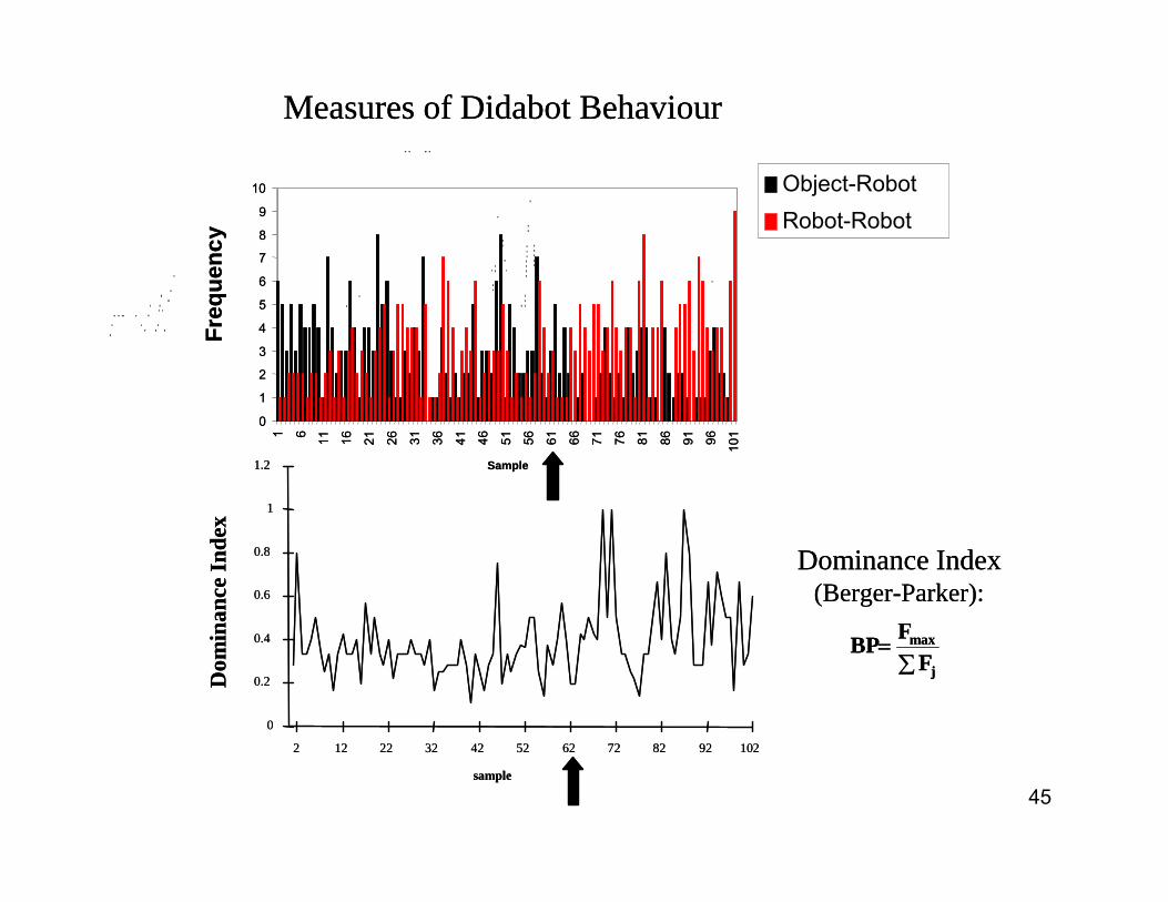
Measures of Didabot Behaviour

Dominance Index(Berger-Parker):

∑=

j

max

FFBP

0

0.2

0.4

0.6

0.8

1

1.2

2 12 22 32 42 52 62 72 82 92 102

sample

Dom

inan

ce In

dex

0

1

2

3

4

5

6

7

8

9

10

1 6 11 16 21 26 31 36 41 46 51 56 61 66 71 76 81 86 91 96 101

Sample

Freq

uenc

yObject-RobotRobot-Robot

Measures of Didabot Behaviour

Dominance Index(Berger-Parker):

∑=

j

max

FFBP

46

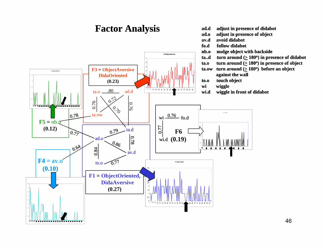
ad.d adjust in presence of didabotad.o adjust in presence of objectav.d avoid didabotfo.d follow didabotnb.o nudge object with backsideta..d turn around (> 180o) in presence of didabotta.o turn around (> 180o) in presence of objectta.ow turn around (> 180o) before an object

against the wallto.o touch objectwi wigglewi.d wiggle in front of didabotta.o ad.d

ta.ow

ta.d

ad.o

av.d

to.o

.800.

76 0.70

0.780.76

0.79

0.86

0.84

0.77

0.72

F5 = nb.o(0.12)

0.78

0.77

F4 = av.o(0.10)

0.64

wi

wi.d

0.77

fo.d0.76

F3 = ObjectAversiveDidaOriented

(0.23)

F1 = ObjectOriented,DidaAversive

(0.27)

F6(0.19)

F3=ObjectAversive

0

1

2

3

4

5

6

7

1 7 13 19 25 31 37 43 49 55 61 67 73 79 85 91 97

F1=DidAv/ObjOr

0

0.5

1

1.5

2

2.5

3

3.5

4

4.5

1 5 9 13 17 21 25 29 33 37 41 45 49 53 57 61 65 69 73 77 81 85 89 93 97

F4=Objec t Av oid

0

0.5

1

1.5

2

2.5

3

3.5

4

4.5

F 2 = WiF o

0

0.5

1

1 .5

2

2 .5

3

3 .5

Nud ge Obje ct

0

0 .5

1

1 .5

2

2 .5

Factor Analysis ad.d adjust in presence of didabotad.o adjust in presence of objectav.d avoid didabotfo.d follow didabotnb.o nudge object with backsideta..d turn around (> 180o) in presence of didabotta.o turn around (> 180o) in presence of objectta.ow turn around (> 180o) before an object

against the wallto.o touch objectwi wigglewi.d wiggle in front of didabotta.o ad.d

ta.ow

ta.d

ad.o

av.d

to.o

.800.

76 0.70

0.780.76

0.79

0.86

0.84

0.77

0.72

F5 = nb.o(0.12)

0.78

0.77

F4 = av.o(0.10)

0.64

wi

wi.d

0.77

fo.d0.76

F3 = ObjectAversiveDidaOriented

(0.23)

F1 = ObjectOriented,DidaAversive

(0.27)

F6(0.19)

F3=ObjectAversive

0

1

2

3

4

5

6

7

1 7 13 19 25 31 37 43 49 55 61 67 73 79 85 91 97

F1=DidAv/ObjOr

0

0.5

1

1.5

2

2.5

3

3.5

4

4.5

1 5 9 13 17 21 25 29 33 37 41 45 49 53 57 61 65 69 73 77 81 85 89 93 97

F4=Objec t Av oid

0

0.5

1

1.5

2

2.5

3

3.5

4

4.5

F 2 = WiF o

0

0.5

1

1 .5

2

2 .5

3

3 .5

Nud ge Obje ct

0

0 .5

1

1 .5

2

2 .5

Factor Analysis

47

F5

F1

F4 F5

0.2F1

0.2

F4

0.2

0.3

0.5

0.1

0.25

F20.1

0.25

0.15 0.25

F3

0.3

0.10.1

0.2 0.1

0.6

0.5

0.2

0.1

1.0

F3 0.7

F20.1

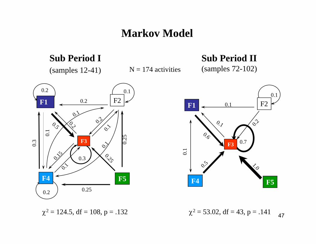
Sub Period I(samples 12-41)

Sub Period II(samples 72-102)

Markov Model0.

1

0.2

0.1

0.1

χ2 = 124.5, df = 108, p = .132 χ2 = 53.02, df = 43, p = .141

N = 174 activities